Embed Size (px)
Citation preview

http://creativecommons.org/licenses/by-sa/2.0/

CIS786, Lecture 4
Usman Roshan

Iterated local search: escape local optima by perturbation
Local optimum
Output of perturbation
Perturbation
Local search
Local search

ILS for MP
• We saw that ratchet improves upon iterative improvement
• We saw that TNT’s sophisticated and faster implementation outperforms ratchet and PAUP* implementations
• But can we do even better?

Disk Covering Methods (DCMs)
• DCMs are divide-and-conquer booster methods. They divide the dataset into small subproblems, compute subtrees using a given base method, merge the subtrees, and refine the supertree.
• DCMs to date– DCM1: for improving statistical performance of
distance-based methods. – DCM2: for improving heuristic search for MP and ML– DCM3: latest, fastest, and best (in accuracy and
optimality) DCM
DCM2 technique for speeding up MP searches
1. Decompose sequences into overlapping subproblems
2. Compute subtrees using a base method
3. Merge subtrees using the Strict Consensus Merge (SCM)
4. Refine to make the tree binary

DCM1 and DCM2 decompositions
DCM1 decomposition : NJ gets better accuracyon small diameter subproblems
DCM2 decomposition:Getting a smaller number of smaller subproblemsspeeds up solution
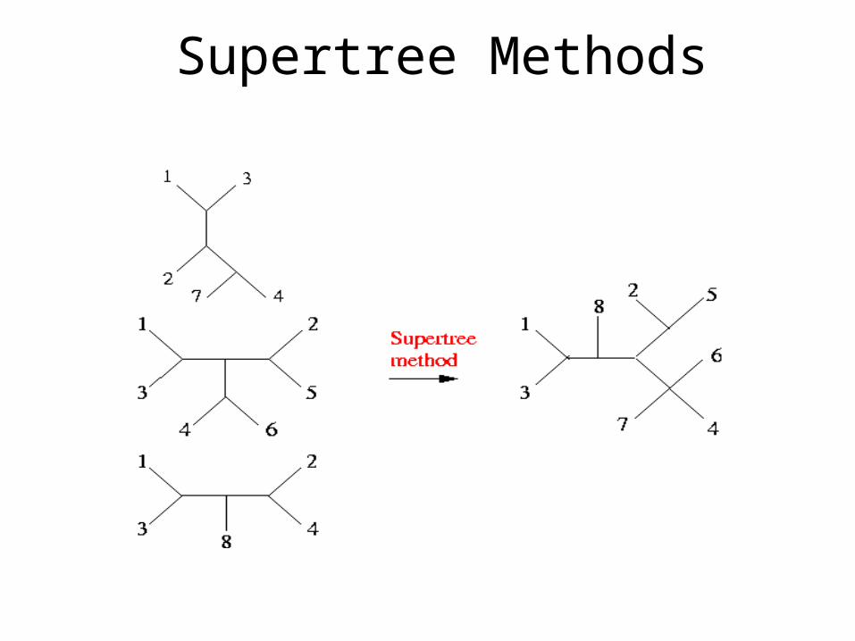
Supertree Methods

Strict Consensus Merger
1 2
3
4 6
5
1 2
3
7 4
1
3
2
4
1 2
3 4
1 2
3 4
1
2
3
4
5
6
7
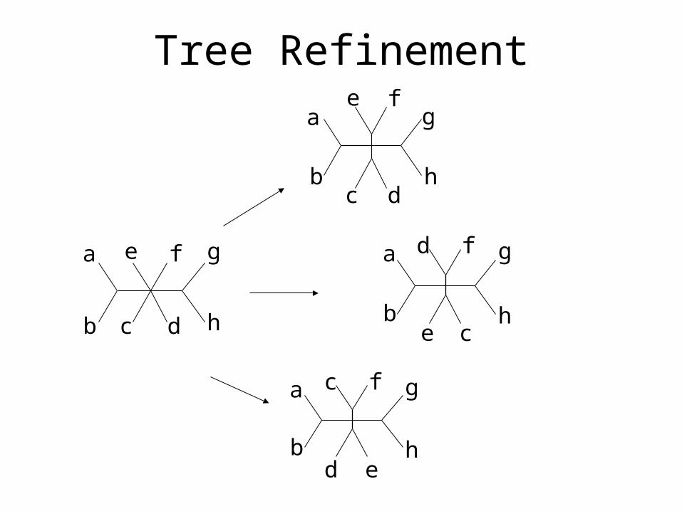
Tree Refinement
ea
b c d
f g
h
a
bc d
fg
h
e
d
e
a
bc
f g
h
a
b
c f g
hd e

The big question
Why DCMs?
Can DCMs improve upon existing
Methods such as neighbor-joining or
PAUP* or TNT?
Improving sequence length requirements of NJ
• Can DCM1 improve upon NJ?
• We examine this question under simulation

DCM1(NJ)
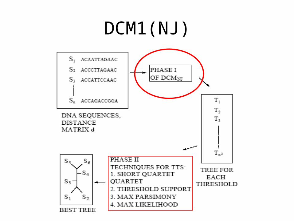
DCM1(NJ)

Computing tree for one threshold

Recall simulation studies

Experimental results
• True tree selection (phase II of DCM1)
• Uniformly random trees
• Birth-death random trees
• Sequence length requirements on birth-death random trees

Comparing tree selection techniques

Error rates on uniform random trees
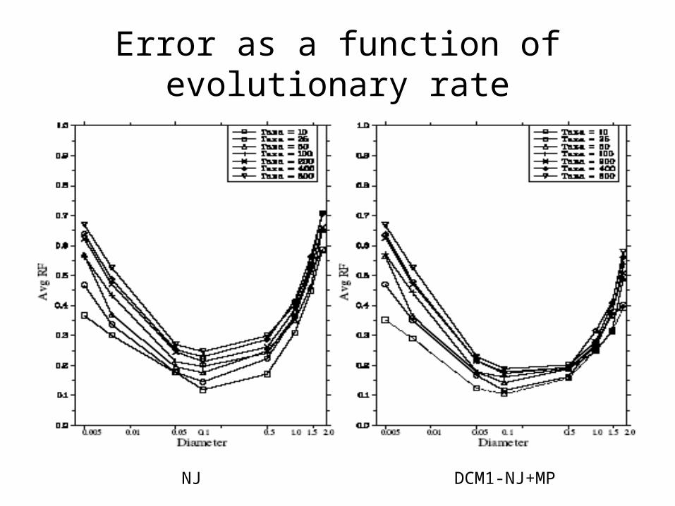
Error as a function of evolutionary rate
NJ DCM1-NJ+MP
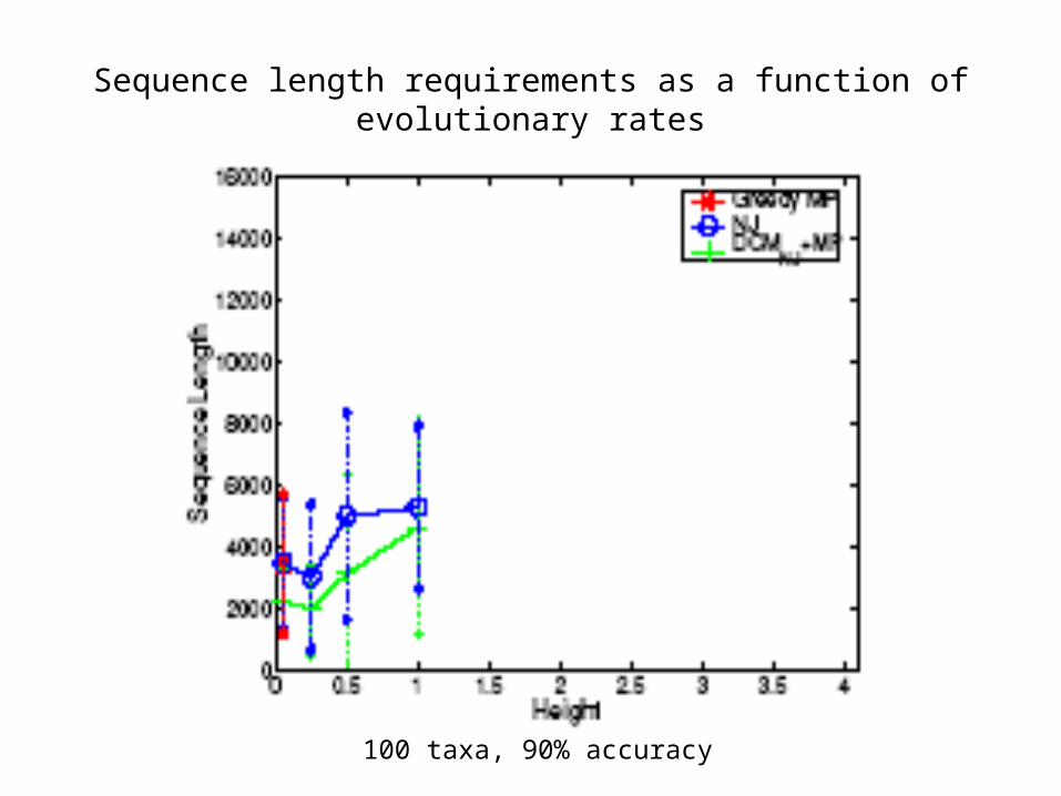
100 taxa, 90% accuracy
Sequence length requirements as a function of evolutionary rates

Sequence length requirements as a function of evolutionary rates
400 taxa, 90% accuracy

Sequence length requirements as a function of #taxa
DCM1-NJ+MP NJ

Conclusion
• DCM1-NJ+MP improves upon NJ on large and divergent settings
• Why did it work?
• Smaller datasets with low evolutionary diameters AND reliable supertree method accurate subtrees (on subsets) accurate supertree

Conclusion
• DCM1-NJ+MP improves upon NJ on large DCM1-NJ+MP improves upon NJ on large and divergent settingsand divergent settings
• Why did it work?Why did it work?• Smaller datasets with low evolutionary Smaller datasets with low evolutionary
diameters AND reliable supertree method diameters AND reliable supertree method accurate subtrees (on subsets) accurate subtrees (on subsets) accurate supertreeaccurate supertree
• But can we improve upon MP heuristics, particularly on large datasets?

Previously we saw a comparison of DCM components for solving MP
• DCM2 better than DCM1 decomposition
• SCM better than MRP (in DCM context)
• Constrained refinement better than Inferred Ancestral States technique
• Higher thresholds take longer but can produce better trees
Comparison of DCM components for solving MP
• DCM2 better than DCM1 decompositionDCM2 better than DCM1 decomposition• SCM better than MRP (in DCM context)SCM better than MRP (in DCM context)• Constrained refinement better than Constrained refinement better than
Inferred Ancestral States techniqueInferred Ancestral States technique• Higher thresholds take longer but can Higher thresholds take longer but can
produce better treesproduce better trees• Can DCM2 improve over TNT? (TNT is
state of the art in solving MP---very fast routines for TBR)
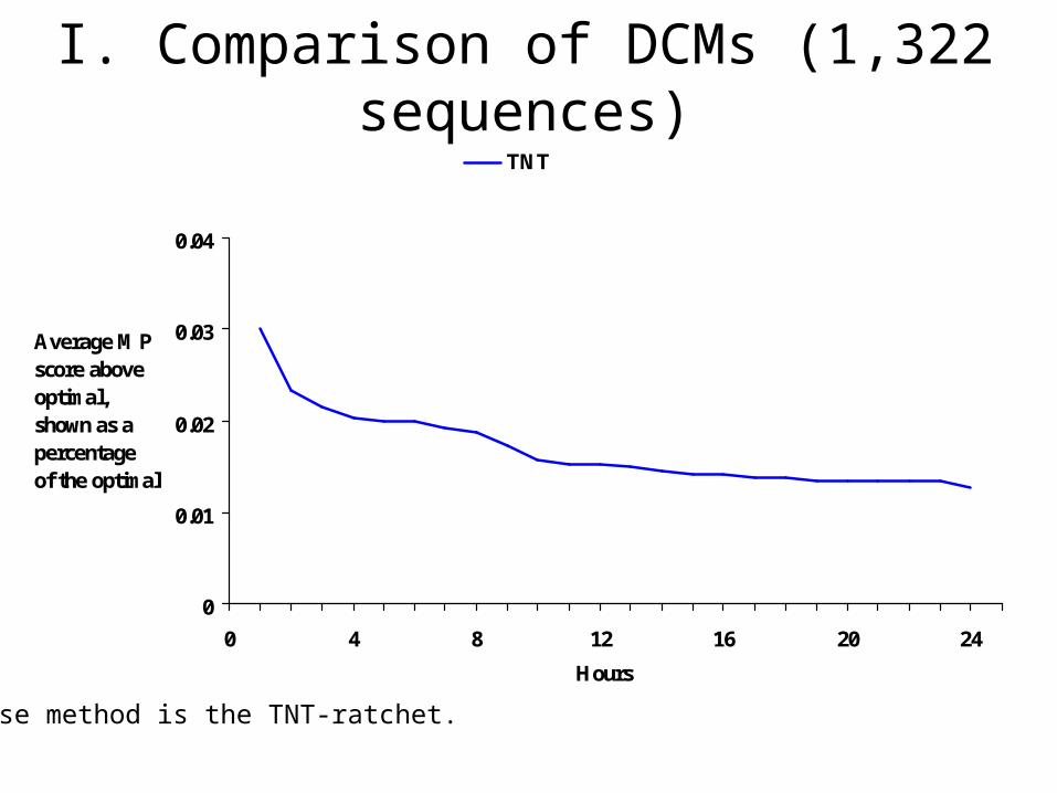
I. Comparison of DCMs (1,322 sequences)
Base method is the TNT-ratchet.
0
0.01
0.02
0.03
0.04
0 4 8 12 16 20 24
Hours
Average MPscore above optimal, shown as a percentage of the optimal
TNT
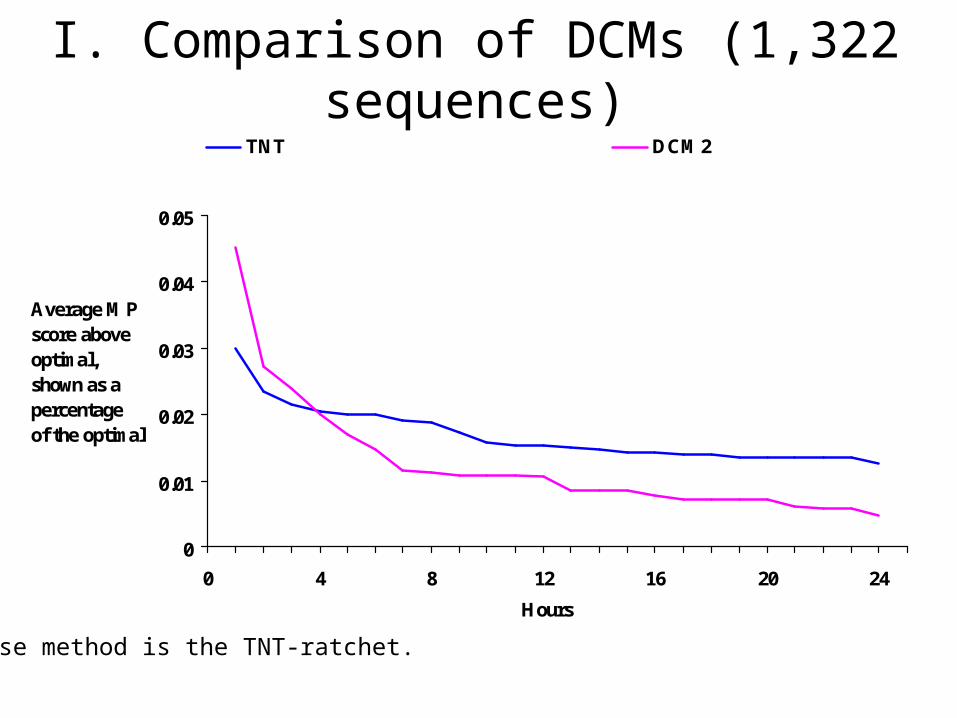
I. Comparison of DCMs (1,322 sequences)
Base method is the TNT-ratchet.
0
0.01
0.02
0.03
0.04
0.05
0 4 8 12 16 20 24
Hours
Average MPscore above optimal, shown as a percentage of the optimal
TNT DCM2

I. Comparison of DCMs (4583 sequences)
Base method is the TNT-ratchet.
0.00
0.05
0.10
0.15
0.20
0.25
0.30
0 4 8 12 16 20 24
Hours
Average MP score above optimal, shown as a percentage of the optimal
TNT

I. Comparison of DCMs (4583 sequences)
Base method is the TNT-ratchet. DCM2 takes almost 10 hours to produce a tree and is too slow to run on larger datasets.
0.00
0.05
0.10
0.15
0.20
0.25
0.30
0 4 8 12 16 20 24
Hours
Average MP score above optimal, shown as a percentage of the optimal
TNT DCM2

DCM2 decomposition on 500 rbcL genes (Zilla dataset)
DCM2 decompositionBlue: separatorRed: subset 1Pink: subset 2
Vizualization produced by graphviz program---draws graph according to specifieddistances.
Nodes: species in the datasetDistances: p-distances (hamming) between the DNAs
1. Separator is very large2. Subsets are very large3. Scattered subsets

Doesn’t look anything like this

2. Find separator X in G which minimizes max where are the connected components of G – X
3. Output subproblems as .
DCM2• Input: distance matrix d,
threshold , sequences S
• Algorithm:1a. Compute a threshold graph G using q and d1b. Perform a minimum weight triangulation of G
DCM3 decomposition
DCM3
• Input: guide-tree T on S, sequences S
• Algorithm:1. Compute a short
quartet graph G using T. The graph G is provably triangulated.
DCM3 advantage: it is faster and produces smaller subproblems than DCM2
iA|| iAX
}{ ijdq
iAX
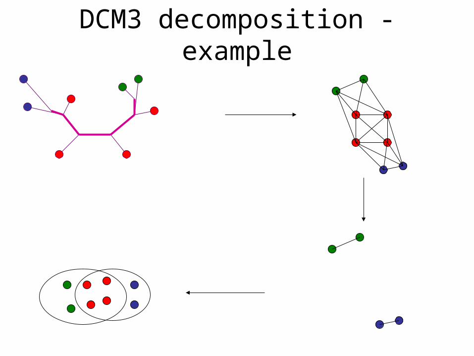
DCM3 decomposition - example

Approx centroid-edge DCM3 decomposition – example
1. Locate the centroid edge e (O(n) time)2. Set the closest leaves around e to be the separator (O(n) time)3. Remaining leaves in subtrees around e form the subsets (unioned with the separator)
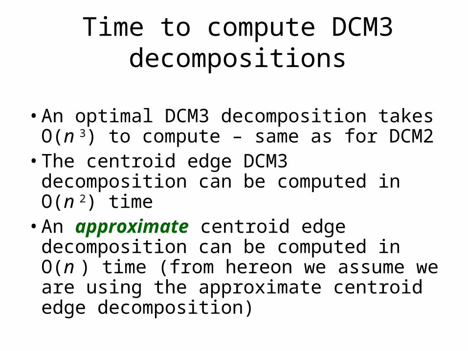
Time to compute DCM3 decompositions
• An optimal DCM3 decomposition takes O(n 3) to compute – same as for DCM2
• The centroid edge DCM3 decomposition can be computed in O(n 2) time
• An approximate centroid edge decomposition can be computed in O(n ) time (from hereon we assume we are using the approximate centroid edge decomposition)

DCM2 decomposition on 500 rbcL genes (Zilla dataset)
DCM2 decompositionBlue: separatorRed: subset 1Pink: subset 2
Vizualization produced by graphviz program---draws graph according to specifieddistances.
Nodes: species in the datasetDistances: p-distances (hamming) between the DNAs
1. Separator is very large2. Subsets are very large3. Scattered subsets

DCM3 decomposition on 500 rbcL genes (Zilla dataset)
DCM3 decompositionBlue: separator (and subset)Red: subset 2Pink: subset 3Yellow: subset 4
Vizualization produced by graphviz
program---draws graph according to
specified distances.
Nodes: species in the datasetDistances: p-distances (hamming) between the DNAs
1. Separator is small2. Subsets are small3. Compact subsets

• Dataset: 4583 actinobacteria ssu rRNA from RDP. Base method is the TNT-ratchet. • DCM2 takes almost 10 hours to produce a tree and is too slow to run on larger datasets. • DCM3 followed by TNT-ratchet doesn’t improve over TNT • Recursive-DCM3 followed by TNT-ratchet doesn’t improve over TNT
Comparison of DCMs
0.00
0.05
0.10
0.15
0.20
0.25
0.30
0 4 8 12 16 20 24
Hours
Average MP score above optimal, shown as a percentage of the optimal
TNT DCM2 DCM3 Rec-DCM3

Local optima is a problem
Phylogenetic trees
Cost
Global optimum
Local optimum

Local optima is a problem
0
0.01
0.02
0.03
0.04
0.05
0.06
0.07
0.08
1 48 96 144 192 240 288 336
TNT
Average MP score above optimal, shown as a percentage of the optimal
Hours

Iterated local search: escape local optima by perturbation
Local optimum
Output of perturbation
Perturbation
Local search
Local search

Iterated local search: Recursive-Iterative-DCM3
Local optimum
Output of Recursive-DCM3
Recursive-DCM3
Local search
Local search

Rec-I-DCM3(TNT-ratchet) improves upon unboosted TNT-ratchet
0.00
0.05
0.10
0.15
0.20
0.25
0.30
0 4 8 12 16 20 24
Hours
Average MP score above optimal, shown as a percentage of the optimal
TNT DCM2 DCM3 Rec-DCM3 Rec-I-DCM3
Comparison of DCMs for solving MP

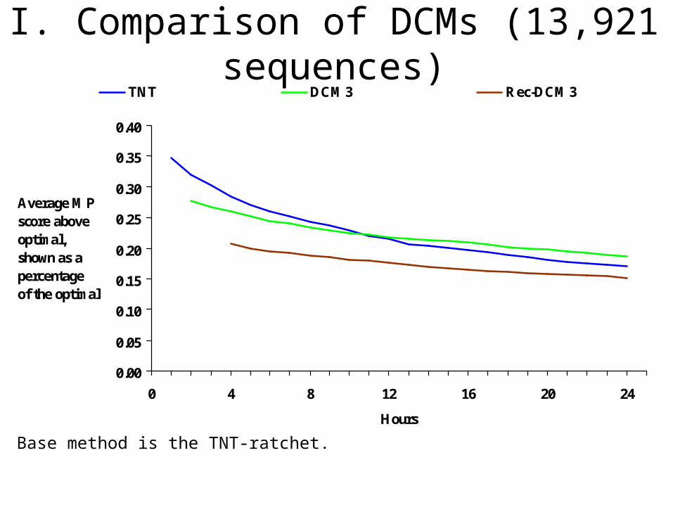
I. Comparison of DCMs (13,921 sequences)
Base method is the TNT-ratchet.
0.00
0.05
0.10
0.15
0.20
0.25
0.30
0.35
0.40
0 4 8 12 16 20 24
Hours
Average MP score aboveoptimal, shown as a percentage of the optimal
TNT
I. Comparison of DCMs (13,921 sequences)
Base method is the TNT-ratchet.
0.00
0.05
0.10
0.15
0.20
0.25
0.30
0.35
0.40
0 4 8 12 16 20 24
Hours
Average MP score aboveoptimal, shown as a percentage of the optimal
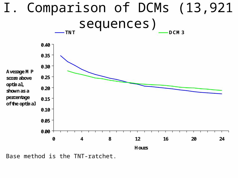
TNT DCM3
I. Comparison of DCMs (13,921 sequences)
Base method is the TNT-ratchet.
0.00
0.05
0.10
0.15
0.20
0.25
0.30
0.35
0.40
0 4 8 12 16 20 24
Hours
Average MP score aboveoptimal, shown as a percentage of the optimal
TNT DCM3 Rec-DCM3
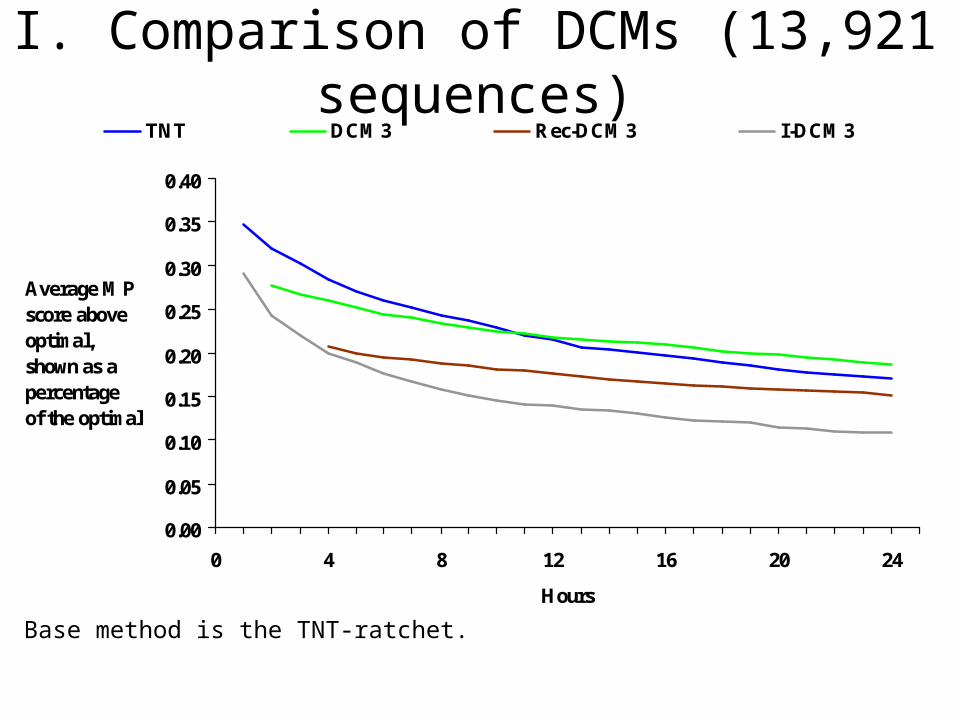
I. Comparison of DCMs (13,921 sequences)
Base method is the TNT-ratchet.
0.00
0.05
0.10
0.15
0.20
0.25
0.30
0.35
0.40
0 4 8 12 16 20 24
Hours
Average MP score aboveoptimal, shown as a percentage of the optimal
TNT DCM3 Rec-DCM3 I-DCM3
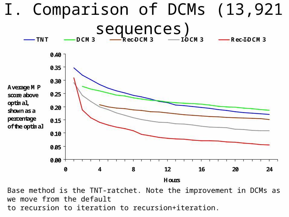
I. Comparison of DCMs (13,921 sequences)
Base method is the TNT-ratchet. Note the improvement in DCMs as we move from the defaultto recursion to iteration to recursion+iteration.
0.00
0.05
0.10
0.15
0.20
0.25
0.30
0.35
0.40
0 4 8 12 16 20 24
Hours
Average MP score aboveoptimal, shown as a percentage of the optimal
TNT DCM3 Rec-DCM3 I-DCM3 Rec-I-DCM3
Improving upon TNT
• But what happens after 24 hours?• We studied boosting upon TNT-ratchet. Other
TNT heuristics are actually better and improving upon them may not be possible. Can we improve upon the default TNT search?
Improving upon TNT
• But what happens after 24 hours?But what happens after 24 hours?• We studied boosting upon TNT-ratchet. Other We studied boosting upon TNT-ratchet. Other
TNT heuristics are actually better and improving TNT heuristics are actually better and improving upon them may not be possible. What about the upon them may not be possible. What about the default TNT search?default TNT search?
• We select some real and large datasets. (Previously we showed that TNT reaches best known scores on small datasets)
• We run 5 trials of TNT for two weeks and 5 of Rec-I-DCM3(TNT) for one week on each dataset
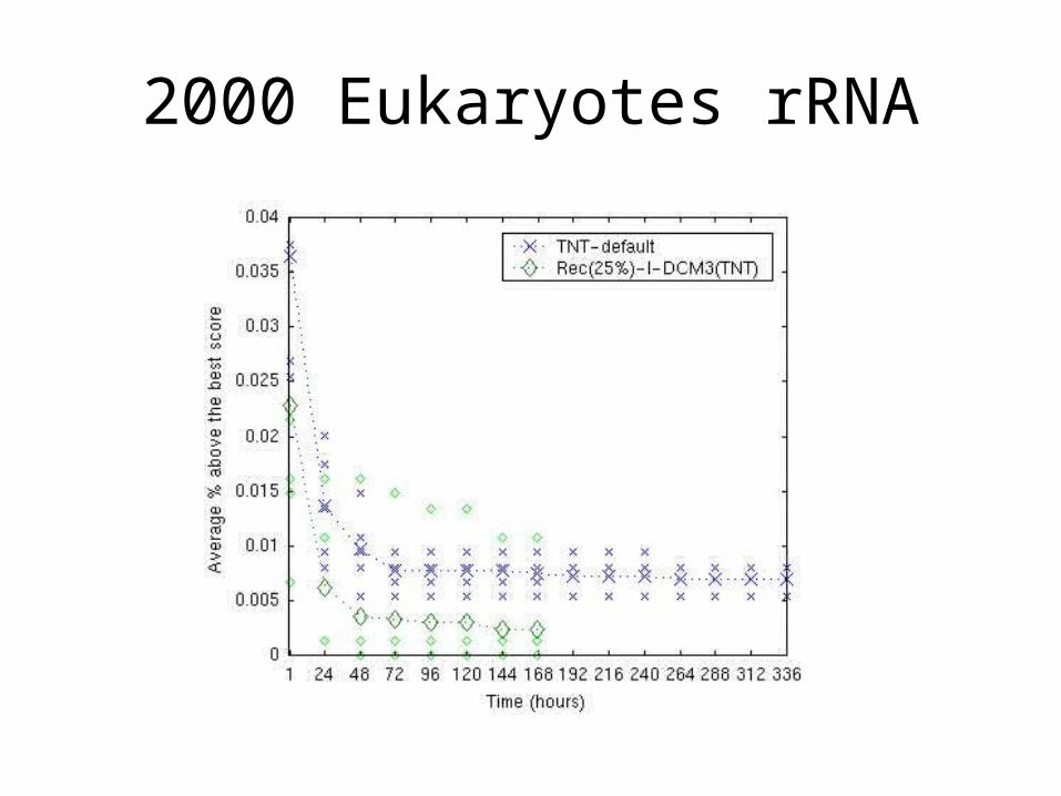
2000 Eukaryotes rRNA

6722 3-domain+2-org rRNA

13921 Proteobacteria rRNA
Improving upon TNT
• What about better TNT heuristics? Can Rec-I-DCM3 improve upon them?
• Rec-I-DCM3 improves upon default TNT but we don’t know what happens for better TNT heuristics.
• Therefore, for a large-scale analysis figure out best settings of the software (e.g. TNT or PAUP*) on the dataset and then use it in conjunction with Rec-I-DCM3 with various subset sizes