HTAP2 status of scenario analysis

Co-ChairsFrank Dentener, PhD Terry Keating, PhD

EC JRC U.S. EPA

2 May 2017

TF HTAP is an expert group organized in 2005 under the UNECE Convention on Long-range Transboundary Air Pollution. Our current work has two main themes:

1. The quantification of global influences on regional air qualityo Driven by the needs of regional air quality planningo Working with AQMEII and MICS-Asia to link modeling at the global and

regional scaleso Developing a foundation for global model evaluation

2. The evaluation of air pollution control opportunities and their impacts at intercontinental to global scaleso Informing the priorities for international cooperation on air pollution

mitigationo Providing information on pollution control opportunities to complement

available regional scale assessments

Evaluation of Air Pollution Controls on Global Scales2012, 2015 Scenarios Workshops at IIASA

• CLE, NFC, MFTR, Climate Policy (via ECLIPSE)

Assessing the Impacts of Future Global Air Pollution Scenarios: Implications for HTAP2, AMAP, and Global IAMs, 17-19 February 2016, IASS, Potsdam, Germany

“Air Quality in a Changing World”; EPA, Chapel Hill, USA, 3-5 April, 2017. • Taking stock of HTAP2 coordinated results• Climate change impacts (with US EPA Star Grants meeting)

Task Force on Integrated Assessment Modeling Annual Meeting, 2-3 May 2017, Paris

• Identification of steps towards enhanced scenario analysis.• Hemispheric Air pollution control strategies

Update of Parameterized S/R Relationships from HTAP1

Development of FASST-HTAP, a screening model for global scenarios

Future Exploration of Health, Ecosystem, and Climate Impacts of Strategies

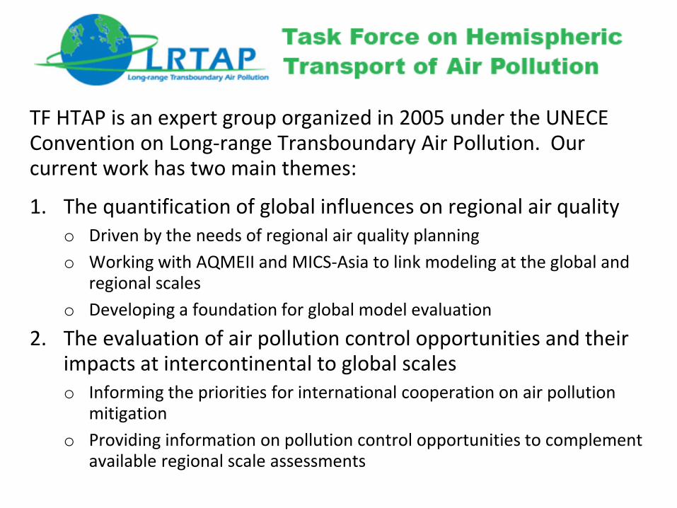
1.Quantification of Global Influences on Regional Air Quality

“Air Quality in a Changing World”; North Carolina, 3-5 April, 2017

2008-10 Global and Regional Modeling Experiments

Atmospheric Chemistry & Physics Global and regional assessment of intercontinental transport of air pollution: results from HTAP, AQMEII and MICS

• 9 articles published in ACP• 6 articles in open review in ACPD• 12 articles in development, more possible• Open to all analyses relevant to quantifying extra-regional

influences• Submission deadline prolonged to 1 December 2017

Overview Report for EMEP/WGE, September 2017

NAEU

EASA

Design of HTAP1 ExperimentsHTAP 2010 Findings

Source-Receptor Sensitivity Simulations: • Present-day emissions, fixed CH4 and 2001 meteorology (base)• Apply 20% reduction to global CH4 burden (1 sensitivity run)• Apply 20% reduction to NOx/VOC/CO/aerosol over each region,

separately and combined (16-20 sensitivity runs)• Additional experiments for dust, fire and anthropogenic aerosol

sources coordinated with the AEROCOM project• Synthetic tracers and detailed analysis of measurement

campaign

Overall Approach: Use global and regional simulations of 2008-2010 to evaluate against observations and to contribute to the quantification of parameterized S/R relationships. Use parameterized S/R relationships to estimate impacts of future strategies.

World divided into 16 Regions (60 sub-regions)7 priority source regions:

North America, Europe, East Asia, South Asia, Russia/Belarus/Ukraine, Middle East

Sensitivity Experiments:Pollutants: CH4, NOx, CO, VOC, aerosol-(precursor)Sectors: Transport; Power/Industry; Residential; Other, Fires/Dust

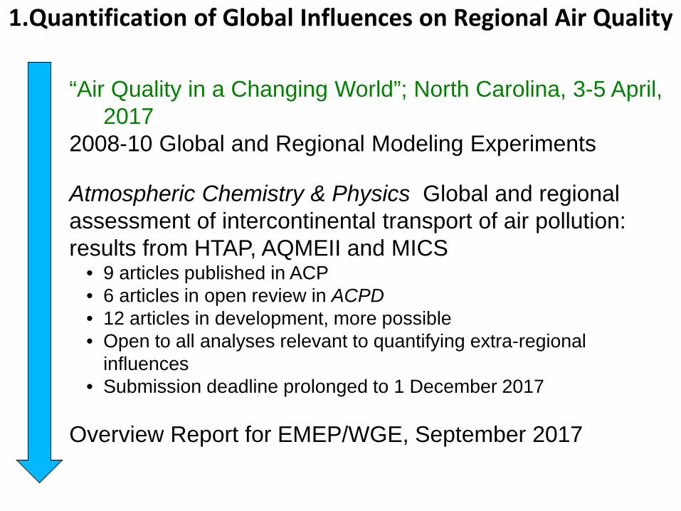
HTAP2 Global & Regional Source/Receptor Modeling

MICSAsia

AQMEIIAQMEII

Nested Regional Simulations from AQMEII and MICS-Asia

HTAP2 Global & Regional Source/Receptor Modeling

23 Base18 GLOALL12 CH4INC12 NAMALL, EURALL, EASALL, SASALL, RBUALL, MDEALL10 GLOCO, GLONOX4 GLOVOC3 GLOPIN, GLORES, GLOTRN (Industry, Residential, Transport)1 Other combinations

A Sparse Matrix of Results for the Global Models:

Model Years for Monthly Average O3 at Model Levels

See Spreadsheet at http://iek8wikis.iek.fz-juelich.de/HTAPWiki/FrontPage(Still missing results from runs that we know have been completed!)

HTAP2 scenario analysis- preliminary findings

• At the HTAP workshop in Chapel Hill a number of model analysis were presented- each with pro’s and con’s

• Basis is a set of ‘HTAP’ (GAINS-ECLIPSEv5a) scenarios.• Next slides show a couple of examples- to get a qualitative

impression of the robustness of the findings. Work in the coming months is needed to corroborate the findings.

• Does the ‘HTAP’ story (‘value of global collaboration on air pollution’) still stand?

Method Pro’s Con’s

HTAP1 SRs- with new scenarios

Published- ca. 15 global models. CLRTAP 2016 report

Large-regions; ‘old’ and coarse resolution models

HTAP2 – scaling of HTAP1 results

New results (ensemble of ca. 5 models); more relevant regions; SR

Sparse matrixMatching HTAP1-HTAP2 regions

TM5-FASST with new scenarios

Widely used (UNEP, CCAC; SSPs)Direct translation in health/vegetation/climate metrics

‘Old’ model resultsMeteo year 2001.Only one model. Linear.

GEOS-Chem Adjoint with new scenarios

Adjoint allows a wide range of analyses (need to define receptor and metric). Used for CCAC.

One model; complicated- not many groups have an adjointversion of their models. Linear.

CAM-Chem colored tracer O3 source attribution; different ‘approach’- additional info

One model- expensive to run- few scenarios. Does not separate the effects of VOCs-CH4- CO

AQMEII regional ensemble Consistency with global models; while higher resolution. Better representation of impact of local emissions.

Driven by single set of Boundary Conditions (ECWMF).Need to understand to what extend differences with global models are ‘improvements’.

Global

Europe

NorthAmerica

East Asia

SouthAsia

Rest ofthe world

NOx NMVOC CO CH4

---- REF CLE Current Legislation- no climate policy---- CLIM-CLE Current legislation-climate policy (IEA 4.5 in the energy sector) REF MFR Maximum Feasible Reductions- no climate policy

There are number of other ‘scenario’ flavors- i.e. focusing on MFR only for the warming SLCFs

HTAP2 / ECLIPSE emissions scenarios as applied in LRTAP Assessment

HTAP1 O3 changes in Europe for HTAP global air pollution scenarios

Total surface O3

change

Within EU

Outside of EU

Methane

REF CLE Current Legislation- no climate policyCLIM-CLE Current legislation- climate policy (energy sector)REF MFR Maximum Feasible Reductions

In Europe: Regional controls can still bring down ozone further, but requires

ambitious and expensive air pollution policy Ambitious air pollution policy elsewhere may be beneficial for

Europe, especially in the US. For the US it would be China, etc.. Methane emission reductions crucial for reducing ozone. Methane is included in climate policies, but we will need to

reduce it also for reducing ozone air pollution. Reducing methane will require strong collaboration with

countries in Asia A likely range for changes in ozone boundary conditions is

therefore estimate to range between -4 and 3 ppb in 2030, and -4 and 5 ppb in 2050.

Does not consider climate change, long-term variability

HTAP2 scenarios- with HTAP1 SR relationship as used in CLRTAP, 2016, Assessment Report

11

TM5-FASSTannual mean surface O3 EUROPE

Annual O3 (ppb)

HTAP1 TM5-FASST

EUR-CLE 2050 + 1 (CH4: +1.5) 3.5 (CH4: + 2)

EUR-MFR 2050

-6 (CH4: -1.5) -3.5 (CH4: -1)

Courtesy, Tim Butler, IASS

CAM-chem: Tagged tracer.HTAP 2010 emissionsAssumes O3 production is NOx limited (implicitly factors in CO, CH4, VOCs)Runs for 2050 – 2 additional scenarios- comparison with SR.

In 2010 winter (Jan) and summer (July) based on tagged tracer and HTAP_v2 2010 emissions:In NW Europe contribution of external O3 is 80 % in winter and 40 % in summerIN E Europe contribution of external O3 is 80 % in winter and 30 % in summer

Adjoint modelling with GEOSCHEMadjoint: O3 linearity as a function of distance from perturbationScenario evaluation is underway.

Experiment: Regional (EAS) TRN perturbations ranging in size

HTAP results for projections based on sectors behave more linear than individual components

Local response Long-range response

Courtesy D. Henze

2050 Results from GEOS-Chem Adjoint

CLE 2050 Surface Daytime Ozone• 30-40 ppb across Europe

Difference between CLE 2050 and CLE 2015• Around 2-3 ppb decrease for most of W. Europe• Little change in E. Europe and isolated spots in

Benelux• Similar to TM5-FASST )

Difference between SLCP Mitigation 2050 and CLE 2050• Additional 3-4 ppb dec available from CH4

mitigation (HTAP1 -1.5 ppb; FASST -2 ppb)

Model results from Daven HenzeInterpretation from T. Keating

2050 Results from GEOS-Chem Adjoint

CLE 2050 Surface Annual PM2.5• 10-30 µg/m3 across Europe?

Difference between CLE 2050 and CLE 2015• 0-8 µg/m3 dec in W. Europe• ~2 µg/m3 inc in Russia and East• Large increase in South Asia

Difference between SLCP Mitigation 2050 and CLE 2050• Up to 4 µg/m3 dec available

Model results from Daven HenzeInterpretation from T. Keating

Perturbation impacts – mortality. AQMEII regional versus global models.

• AQMEII3 Regional Models (5) HTAP2 Global Models (Liang et al., 2017)

* Sum of 6 source regions• Error bars estimated from ensembles of CTM model results• Difference for Europe/NAM case attributable to severe underestimation of PM2.5 in

winter time by all reg. models which used the same global model for BC

Source Receptor

Europe United States

GLO -54 000 [-74000 ;-39000] -27500 [-38000; -12000]

NAM -81 [-736; 250] -25000 [-36000; -12000]

EUR -47 000 [-72000;-25000] -

EAS - -1900 ± [-4400; -440]

Source Receptor

Europe United States

GLO* -38 930 [-61000; -1 600] -20 610 [-33000; -2 800]

NAM -1 150 [-2150; -50] -19 720 [-31000; -3 000]

EUR -34 230 [-53 000; -1700]

EAS -530 [-1100 -30]

Premature Death External Cost

Europe 414 000 ± 98 000 400 billion €

USA 158 000 ± 74 000 136 billion €

Multi-model assessment of health impacts of air pollution using AQMEII dataset and EVA (Aarhus University) shows an approximately factor of 3 difference in premature deaths between Europe and US.

ConclusionsNew HTAP2 emission perturbation studies: new SR regions; and ‘sparse matrix’ of simulations makes it more difficult to come up with a straight forward analysis of hemispheric contributions

Several other analysis methods using the same 2010 emission database (HTAP_v2 or ECLIPSE emission for scenarios) provide qualitatively consistent results with regard to extra-regional contributions and O3 scenario envelop until 2050.

The ‘HTAP’ story: ‘value of cooperation’ still stands - probably even stronger because of a larger differences in emissions trends in developed and developing countries.

Most likely way forward is to use updated SRs, which will be a mix of HTAP1 and HTAP2 as the central tool and use the results from other models as well as regional models to assess uncertainties. Differences can be narrowed down. Regional models for health impact assessment?

In the next months we’ll try to reach convergence on the best way to move forward.

Process is driven by the ACP special issue - new deadline 01.12.2017

Method Pro’s Con’s

HTAP1 SRs- with new scenarios

Published- ca. 15 global models. CLRTAP 2016 report

Large-regions; ‘old’ and coarse resolution models

HTAP2 – scaling of HTAP1 results

New results (ensemble of ca. 5 models); more relevant regions; SR

Sparse matrixMatching HTAP1-HTAP2 regions

TM5-FASST with new scenarios

Widely used (UNEP, CCAC; SSPs)Direct translation in health/vegetation/climate metrics

‘Old’ model resultsMeteo year 2001.Only one model. Linear.

GEOS-Chem Adjoint with new scenarios

Adjoint allows a wide range of analyses (need to define receptor and metric). Used for CCAC.

One model; complicated- not many groups have an adjointversion of their models. Linear.

CAM-Chem colored tracer O3 source attribution; different ‘approach’- additional info

One model- expensive to run- few scenarios. Does not separate the effects of VOCs-CH4- CO

AQMEII regional ensemble Consistency with global models; while higher resolution. Better representation of impact of local emissions.

Driven by single set of Boundary Conditions (ECWMF).Need to understand to what extend differences with global models are ‘improvements’.