HSTS: Integrating Planning and Scheduling

Nicola Museettola

CMU-RI-TR-93-05

The Robotics Institute Camegie Mellon University

Pittsburgh, Pennsylvania 15213

March 1993

To appear in Intelligent Scheduling, Mark S . Fox and Monte Zweben (editors), Morgan Kaufmann, 1993.

0 1993 Carnegie MelIon University

This work was sponsored in part by the National Aeronautics and Space Administration under contract # NCC 2-707, &be Defense Advanced Research Projects Agency under contract #F30602-91-F-0016, and the Robotics Institute.

Table of Contents 1 Introduction 2 Two application domains

3 Integration of planning and scheduling 4 The fundamental components of HSTS

4.1 Domain Description Language 4.2 Temporal Data Base

5 Additional HSTS features 5.1 Sequence Constraints 5.2 Time and type consistency

6.1 Atomic State Variables 6.2 Aggregate State Variables

2.1 Space Mission Scheduling 2.2 Transportation Planning

6 Managing Resources

7 Scheduling the Hubble Space Telescope 8 Exploiting temporal flexibility in scheduling

8.1 Conflict Partition Scheduling 8.2 Experimental evaluation

8.2.1 Experimental design 8.2.2 Experimental mults

9 Conclusions Acknowledgments References

1 2 2 4 5 6 6 8

12 12 13 15 15 16 17 20 21 25 25 26 28 30 31

List of Figures Figure 1: The Hubble Space Telescope domain Figure 2: Value transition graph for state(POINTING-DEVICE). Figure 3: Compatibilities for the value LOCkXD(?T). Figure 4: Insertion of a value token into a time Lie. Figure 5: Implementation of a contained-by compatibility Figure 6: A sequence compatibility. Figure 7: Implementation of a sequence compatibility. Figure 8: A time point network. Figure 9: Type propagation on a time line. Figure 1 0 Posting a sequence constraint on an aggregate state variable. Figure 11: Initial activity network. Figure 12: Bottleneck resource status before scheduling cycle. Figure 13: Activity network after Conflict Arbitration. Figure 14: New bottleneck resource status.

3 8 8

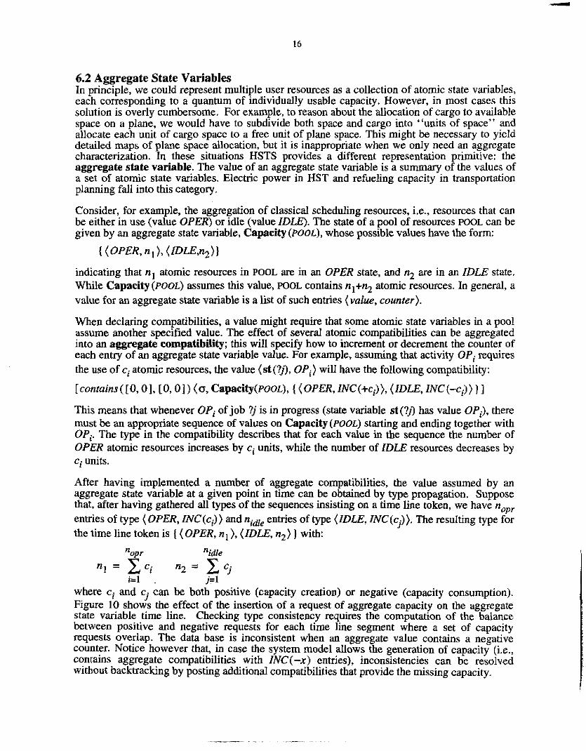
10 11 12 13 14 14 17 24 24 25 25

... 111

List of Tables Table 1: Performance results. The times are reported in hours, minutes, 20

seconds, and fractions of second. Table 2: Comparative results: number of problems solved. 27 Table 3: Comparative results: CPU time. 28

Abstract

In the traditional approach to managing complex systems, planning and scheduling are two very distinct phases. However, in a wide variety of applications this strict separation is not possible or beneficial. During scheduling it is often necessary to make planning decisions (plan the setup of a machine); moreover planning decisions can benefit from scheduling information (choose a process plan depending on resource loads). HSTS (Heuristic Scheduling Testbed System) is a representation and problem solving framework that provides an integrated view of planning and scheduling. HSTS emphasizes the decomposition of a domain into state variables evolving over continuous time, This allows the description and manipulation of resources far more complex than it is possible in classical scheduling. The inclusion of time and resource capacity into the description of causal justifications allows a fine-grain integration of planning and scheduling and a better adaptation to problem and domain structure. HSTS puts special emphasis on leaving as much temporal flexibility as possible during the planninghcheduling process to generate better pldschedules with less computation effort. Within the HSTS framework we have implemented several planninghcheduling systems. In the paper we describe an integrated planner and scheduler for short term scheduling of the Hubble Space Telescope. This system has demonstrated the ability to deal effectively with all of the important constraints of the domain. Experimental results show that executable schedules for Hubble can be built in a time compatible with operational needs. The paper also describes a methodology for job-shop scheduling problems. The methodology exploits the temporal flexibility provided by HSTS. Experimental results show that this approach is more effective than other intelligent scheduling techniques in the solution of scheduling problems with non-negotiable dead-lines.

1

1 Introduction In the traditional approach to managing complex systems, planning and scheduling are two very distinct phases. Planning determines how the system achieves different types of goals. The process consists of concatenating elementary transformations (or actions) to move the world into a state that satisfies the goal. The result is a library of plans. Scheduling takes responsibility for day to day operations. After receiving a set of goals, a scheduler instantiates plan templates contained in the library and assigns to each action a time slot for the exclusive use of the needed resources. The result is the prediction of a specific course of action that, if followed, ensures the achievement of all goals within the system’s physical constraints.

A typical case is the management of a manufacturing facility. Planning develops processes to manufacture given product types (e.g., -transforming a raw block of metal into a widget). Scheduling receives a number of orders to produce widgets of given types with known release dates for raw materials and due dates for finished products. In both phases, costs should be kept as low as possible; this might require generating processes with a minimum number of steps, or scheduling the last action in each order as close as possible to the due date.

This strict separation between planning and scheduling does not match the operating conditions of a wide variety of complex systems. Even in cases where separation is viable it might be overly restrictive. A more flexible adaptation to the structure of the problem might yield better solutions. For example, during the scheduling phase it is often necessary to expand setup activities; these are not justified by the achievement of a primary goal but depend exclusively on how other activities are sequenced on a resource. Consider an instance where two sequential operations require drilling holes of different diameters using the same drilling machine; the schedule must allocate time for the substitution of the drill bit. In other situations, planning might be profitably delayed into the scheduling phase. This allows the expansion of courses of action that, although a priori sub-optimal, are clearly convenient when considering expected resource usage. The number of possible alternatives might make the management of a complete plan library impractical as required by the traditional approach.

A major obstacle to more integrated and flexible planning and scheduling is the lack of a unified framework. This should support the representation of all aspects of the problem in a way that makes the inherent structure of the domain evident. When dealing with large problems and complex domains, a framework with strong structuring devices facilitates the decomposition of system models and the consequent management of the combinatorics of search.

In planning, most Artificial Intelligence research adopts the classical representational assumption proposed by the STRIPS planning system [IO]. In this view action is essentially an instantaneous transition between two world states of indeterminate durations. The structural complexity of a state is unbound, but the devices provided for its description are completely unstructured, such as complete first order theories or lists of predicates. Some frameworks [40,38] have demonstrated the ability to address practical planning problems. However, the classical assumption lacks balance between generality and structure; this is a major obstacle in extending classical planning into integrated planning and scheduling. Past research has attempted partial extensions in several important directions: processes evolving over continuous [2] and metric time [39,7], parallelism [20], and external events [13]. However, no comprehensive view has yet been proposed to

address the integration problem.

Classical scheduling research has always exploited much stronger structuring assumptions [3]. Domains are decomposed into a set of resources whose states evolve over continuous time. This facilitates the explicit representation of resource utilization over extended periods of time. Several current scheduling systems exploit reasoning over such representations f11.36, 32,22,42,5]. Empirical studies have demonstrated the superiority of this approach L29.321 with respect to dispatching scheduling [30], where decision making focuses only on the

2

immediate future. However, the scheduling view of the world has very strong limitations. No information is kept about a resource state beyond its availability. Additional state information (e.g., which bit is mounted in a drill at a given time) is crucial to maintain causal justifications and to dynamically expand support activities during problem solving.

In this chapter we describe HSTS (Heuristic Scheduling Testbed System), a representation and problem solving framework that aims at unifying planning and scheduling. Similar to classical scheduling, HSTS decomposes a domain into a vector of state variables continuously evolving over time. Similar to planning, HSTS provides general devices for representing complex states and causal justifications. Within this framework we have developed and experimentally tested planninghcheduling systems for several unconventional domains. These domain include short term scheduling for the Hubble Space Telescope [25] and “bare base” deployment for transportation planning [12]. Several constraint propagation mechanisms support the richness of domain representation at any problem solving stage.

Schedules developed in HSTS implicitly identify a set of legal system behaviors. This is an important distinction with respect to classical approaches which, instead, specify all aspects of a single, nominal system behavior. During execution, a nominal behavior is interpreted as an ideal trajectory to be followed as closely as possible. However, since the schedule does not explicitly represent feasible alternatives, it is difficult to have a clear picture of the impact of the unavoidable deviations from the desired course of action. HSTS, instead, advocates schedules as envelopes of behavior within which the executor is free to react to unexpected events and still maintain acceptable system performance. Viewing scheduling as the manipulation of behavior envelopes has potential advantages during pldschedule construction. In this chapter, we will discuss a heuristic scheduling methodology, Conflict Partition Scheduling (CPS), that operates on a temporally flexible network of constraints under the guidance of statistical estimates of the network’s properties. We will show experimental evidence of CPS’s superiority with respect to other intelligent scheduling approaches.

The chapter is organized as follows. In section 2 we briefly describe two unconventional application domains that require integrated planning and scheduling. We then introduce the basic HSTS modeling principle which allows such integration (section 3). A detailed description of the features of HSTS follows in sections 4 and 5. Special attention is given to the wide variety of resource capacity constraints supported by the framework (section 6). The rest of the chapter describes two problem solvers implemented in HSTS: a short-term scheduler for Hubble Space Telescope observation scheduling (section 7) and a scheduling methodology for job-shop scheduling (section 8). In the conclusions (section 9) we summarize the status of the project and discuss future research directions.

2 Two application domains

2.1 Space Mission Scheduling Space mission scheduling problems include managing orbiting astronomical observatories, coordinating the execution of activities aboard the space station, and generating detailed command sequences for automated planetary probes. These apparently diverse applications share two main sources of complexity. The first is the need to use the space facility with high efficiency in the presence of a very large number of diverse usage requests. Much of the international scientific community is eager to take advantage of the unique conditions found in space (e.g., weightlessness, extreme vacuum, exposure to radiation that does not reach the surface of the earth). For example, in the case of the Hubble Space Telescope, the number of individual observations requested over a year is on the order of several tens of thousands. Consequently, the time requested by the experiments deemed worth pursuing exceeds the

3

A I

Recorder Tape -

lifetime of any given mission. To maximize return, the final schedule must accommodate as many of these experiments as possible. The second source of complexity is the need to insure a safe operation of the space facility. It is not enough to allocate exclusive time for the execution of main activities; the schedule must contain enough detail to explicitly ensure that auxiliary reconfigurations and intermediate states of the various subsystems do not interact in a harmful way.

A typical space mission scheduling problem is the generation of short-term schedules for the Hubble Space Telescope (HST). Astronomers formulate observation programs according to a fairly sophisticated specification language [37]. The basic structure of each program is a partial ordering of observations. Each observation specifies the collection of light from a celestial object with one of the telescope’s scientific instruments. A program can contain a diverse set of temporal constraints including precedences, windows of opportunity for groups of observations, minimum and maximum temporal separations, and coordinated parallel observations with different viewing instruments. When executing an observation, HST gathers light from celestial objects called targets, and communicates scientific data back to Earth through one of two TDRSS communication satellites (Figure I). Given the telescope’s low altitude orbit, the Earth periodically occludes virtually any target and communication satellite. The fraction of orbit during which each of them is available for observation or communication depends on their position.

Hubble Space Telescope

-

Data Path

. Communication

Scientific Instruments

I

Targets

Receiving Devices

Figure 1: The Hubble Space Telescope domain

The telescope subsystems must be operated paying continuous attention to several stringent constraints. These include limited available electric power, and maintenance of acceptable temperature profiles on the telescope structure. The pointing subsystem is responsible for orienting HST toward a target, and locking it at the center of the field of view of the designated

A

scientific instrument. HST has 6 different scientific instruments, but available electric power does not allow all of them to be operational simultaneously. Moving an instrument between operation and quiescence requires complex reconfiguration sequences which must be coordinated among various instrument components. Reconfigurations must also be appropriately synchronized among different instruments. Data can be read from the instruments and directly communicated to Earth through one of two links operating at different communication rates; it can also be temporarily stored on an on-board tape recorder and communicated to Earth at a later time.

In summary, solving the HST observation scheduling problem requires the generation of command sequences to accommodate as many observations as possible while maintaining telescope integrity and satisfying constraints and preferences imposed by the scientists.

2.2 Transportation Planning Disaster relief operations or other large-scale responses to international crises require. the coordination of the transportation of a large number of people, goods, and other facilities. For example, transportation plans to support military operations are very large, and involve the movement of tens of thousands of individual units. These units span a diverse range of size and composition: from a single person or piece of cargo to an entire division [14]. The timely execution of a well-coordinated transportation plan is crucial for the success of an operation.

Units can use transpoaation resources (e.g., planes, ships) depending on their original location, their intended destination, and the time at which they are needed at the destination. Therefore, it is not sufficient for a unit to fmd a resource with enough transportation capacity at the appropriate time, but the resource’s mute must also match the unit’s source and destination locations. Units can be assigned to transportation flows already established. In case their arrival at the destination is extremely critical, transportation resources can be diverted from other less critical uses or temporarily acquired from other sources (e.g., planes chartered from commercial airlines). Justification information includes mutual dependency among different unit deployments and intended effects of a unit becoming operational at the destination. Keeping track of this information is essential in order to adapt the plan to unexpected execution conditions or to partially reuse it in other situations.

Often the primary goal served by a unit is to augment the facilities available at the destination, so as to increase its throughput and to allow a higher rate of delivery. Typical examples of these facilities are air traffic control, aircraft refueling, and personnel or cargo unloading. Aggregate capacity resources are often an appropriate representation for these facilities. The state of an aggregate resource represents capacity in use or still available at any point in time. To make a more concrete example, let us consider a “bare base” scenario, where the goal is to turn a bare runway at the destination into a fully functioning airport. The number of planes that can be refueled in parallel at the destination can be represented as an aggregate refueling capacity. Bringing in one or more refueling units permanently increases refueling capacity. Since planes use this facility immediately after arrival, increasing refueling capacity increases the plane arrival rate at the destination. This in turn increases the arrival rate of additional refueling units, resulting in a quick amplification of the capabilities of the airport. Increasing the number of units at a site also increases the demand for other supporting functions (such as sleeping space, food, and fuel) which are provided by other units. The arrival of these additional units must be carefully coordinated to avoid chaotic situations and negative consequences on the overall outcome of the mission.

In conclusion, the salient factors in transportation planning are time, dynamic generation and consumption of several types of aggregate capacity, state information, and causal relations. This domain is a primary candidate for the application of integrated planning and scheduling.

5

3 Integration of planning and scheduling To deal effectively with complex domains we need a synthesis of the problem solving capabilities currently split between classical planning and classical scheduling. To this end, it is crucial to recognize that a domain can always be described as a dynamical system[17]. A dynamical system is a formal structure that gives the relationship between exerted actions (input) and observed behaviors over time, taking into account the internal memory of past history (sfare).* Planning and scheduling are in fact complementary aspects of the process of step-by- step construction of consistent dynamical system behaviors [23, 81. To build a problem solving framework capable of easily accommodating this process we must choose an appropriate structuring principle for the description of the dynamical system.

In domains like space mission scheduling and transportation planning we can accurately describe the system’s instantaneous situation with the value of a handful of its properties (e.g., the operative state of each component of the space telescope, the usage of different airport facilities). Therefore, we adopt the fundamental structuring principle of describing both input and state as finite dimensional vectors of values evolving over continuous time. The same principle is adopted by approaches that deal with continuous value dynamical systems (e.g., linear systems) [17] and with the temporal specification of reactive software systems [21].

The input and state vector assumption promotes a more general view of the domain than those allowed by classical scheduling and planning.

Classical scheduling requires the representation of resources. A vector component can directly model a single capacity resource since it can assume one and only one value at any point in time. In this case the range of possible values is essentially binary (e.g., processing or d e ) . However, in our representation the range of vector component values can be wider than binary, allowing the inclusion of more complex state information into the representation of resources. This extends the restrictive assumptions made in classical scheduling.

In classical planning, the evolution of a domain strictly alternates between a stage of change (ucrion) and a period of static persistence (sfare). A representation based on input and state vectors promotes a different view. The input vector identifies those system properties directly controlled by an external agent, while the state vector refers to those which can only be indirectly influenced. Values representing change and persistence can appear in any order in any vector component. For example, it is possible to have static values one immediately after the other (when transitions have infmitesimal durations) or changes following one another (when a process is divided into two or more contiguous phases). This facilitates reasoning over parallel processes evolving over continuous time.

In the rest of the paper we will discuss only state vectors, assuming that for the domains of interest the synthesis of the input is straightforward (e.g., sending the signal to start an operation on a resource at a time determined by the schedule).

These modeling premises also support the formulation of a broader class of problems than those usually expressible in classical planning and scheduling. A planning/scheduling problem is simply a set of constraints and preferences on state vector values; their satisfaction identifies a desired pladschedule among all possible consistent behaviors. Constraints can specify both the execution of actions, as in classical scheduling, and the request for stationary states, as in classical planning. Evaluation functions can impose preference on the possible behaviors of the system (e.g., execute as many observations as possible out of a pool submitted to HST). A good planner/scheduler will try to constmct behaviors with a high (possibly globally maximal) level of

*In the following we will identi& the observable behavior of the system with the evolution of its state over time.

6

satisfaction for these preferences.

4 The fundamental components of HSTS The HSTS framework makes coherent use of the previous representational principle. The two core components are the Domain Description Language (HSTS-DDL) and the Temporal Data Base (HSTS-TDB). HSTS-DDL allows the specification of the static and dynamic structure of a system. It supports the expression of a model as a modular set of constraint templates satisfied by any legal system behavior. HSTS-TDB supports the construction of such legal behaviors. It provides facilities to insure a strict adherence of its content to an HSTS-DDL system model and to any requirement stated in a problem. By posting assertions and constraints among assertions in the data base, a planner/scheduler sets goals, builds activity networks, commits to the achievement of intermediate states, and synchronizes system components. The tight connection between the entities that can be specified in HSTS-DDL and those that can be represented in HSTS-TDB provides a strong basis for exploiting domain structure during problem solving.

4.1 Domain Description Language An HSTS-DDL system model is organized as a set of system components, each with an associated set of properties. Each property represents an entry of the state vector; it can therefore assume one and only one value at any point in time. Properties whose value does not change over time (also called static properties) typically represent system parameters. The behavior of the system is determined by the value of its dynamic properties, those that change over time; in the rest of the paper we will refer to them as the state variables of the system.

HSTS-DDL gives special emphasis to the specification of state variables. A system model must explicitly declare the set of all possible values for each state variable. A value is expressed as a predicate R ( x l , x2, ....., xn) , where <nl, 2, ....., xn> is a tuple in the relation R. The model must give a domain for each predicate’s argument; currently HSTS-DDL allows sets of symbols, sets of system components, and numeric quantities (either discrete or continuous).

To illustrate these points we give an example from HST. The system component POINTING-DEVICE has several properties. One of them is the telescope’s average slewing rate, described as a constant value of a static property. The pointing direction of the telescope and the state of target tracking is determined by a single state variable, State(POr”G-DEVICE). Its possible values are:

UNLOCKED ( ?T) : the telescope is pointing in the generic direction of target ?T;

LOCKED( ?T) : the telescope is actively tracking target ?T;

LOCKING( ?T) : the tracking device is locking onto target ?T;

SLEWING(?Tl, ?Z2) : the telescope changes its direction from target ?TI to target ?72.

The domain of each of the variables ?T, ?TI and ?T2 is the set of all known targets, each represented as a separate system component in the HST model.

The specification of each state variable value is incomplete without its temporal characteristics. For a system behavior each value extends over a continuous time interval or occurrence. A value’s occurrence depends in part on the value’s intrinsic characteristic and in part on its interaction with other values. For example, the duration of a slewing operation is entirely determined by intrinsic parameters, like the angle between the two targets and the telescope’s slewing rate. On the other hand, the only cause for the telescope to exit an unlocked state is the

Occurrence of either a slewing or a locking operation, i.e., the interaction with other values.

In HSTS-DDL each value has a duration constraint which expresses the intrinsic range [d , D ] of its possible durations (D 2 d2 0); d and D are respectively the duration’s lower and upper bounds. The bounds are specified as functions of the value’s arguments; their tightness depends on the binding status of the value’s arguments. For example, during problem solving ?T1 and ?72 in SLEWING(?Tl, ?n) might be restricted to specific sets of targets. The lower bound of the duration constraint would return the slewing time between the closest pair of targets, each selected from a different set; the upper bound would refe.r to the farthest pair of targets. If each of ?T1 and ?72 are restricted to a single target, both the lower and upper bounds will assume the slewing time between the two targets.

For any system it is possible to identify constraining patterns of value occurrences. In any legal behavior, when a value occurs other values must also occur to match the pattern. Such patterns describe the dynamic characteristics of the system, and have a function similar to state operators in classical planning. In HSTS-DDL each value is constrained by a compatibility specification which consists of a set of compatibilities organized as an AND/OR graph. Each compatibility represents the request for an elementary temporal constraint between the value and an appropriate segment of behavior. More precisely, a compatibility has the form:

[ temp-rel <comp-class, st-vur, type >]

The tuple < comp-class, st-vur, type > specifies the characteristics of a constraining segment of behavior; temp-rel is the temporal relation requested between the constrained value and the constraining segment of behavior. The temporal relations known to HSTS-DDL are equivalent to all combinations of interval relations[l] with metric constraints that can be expressed in continuous endpoint algebra [IS]. For example, before( [d , D]) indicates that the end of the constrained value must precede the start of the constraining behavior segment by a time interval 6, such that d 5 6 I D ; its inverse is ufrer([d,D]) . The relation contained-by( [ d l , D 1 ] , [d2, D2]) says that the constrained value must be contained within the constraining behavior segment; [d,, D 1 ] defines the distance between the two start times while [d2, D2] refers to the two end times. HSTS-DDL restricts the constraining behavior segment to occur on a single state variable, st-vur. The identifier comp-class can be one of two symbols, v or 6, depending on the nature of the behavior segment. The symbol v stands for a single value occurrence (value compatibility), while D refers to a sequence of values occurring contiguously on the same state variable (sequence compatibility). In this section we describe value compatibilities; section 5.1 will discuss sequence compatibilities. The behavior segment must consist of values extracted from the set specified in type.

To draw an illustrative example from the HST domain, let us consider the dynamic state of the telescope’s pointing device (state variable ~~&(POI”G-DEVICE)). The possible value transitions are shown in figure 2. Each node represents one of the possible values while an arc between two nodes represents two compatibilities. More precisely, an arc from node ni to node nj is equivalent to a [before( [0, 01 ) < v, state(PoIWfNGDEWCE), Inj} > ] compatibility associated to ni, and to a symmetric ufer([O,O]) compatibility associated to nj. Multiple arcs exiting or entering a node correspond to alternative transitions (OR node in the compatibility specification). Some of the values can persist indefinitely (highlighted nodes in figure 2) and have therefore an indeterminate duration constraint ([0, fm] bound); all other values have a determined duration constraint, To precisely specify the physically consistent patterns of behavior, we must also consider synchronization with other state variables. For example, locking the telescope on a target and keeping the lock requires target visibility. This imposes an additional compatibility ([canruzned-by( [0, +-I, [0 , + - I ) < v, visibility(?n, [ VISIBLE] >]) on each of the values WCKING(?T) and LOCKED(?T). Figure 3 lists the complete

8

compatibility specification for LOCKED( ?T).

LOCKING

UNLOCXED 6 W

SLEWING

Figure 2: Value transition graph for ~~~~~(POINTING-DEVICE).

< state ( POINTING-DEVICE ), LOCKED ( ?T ) >

1 contained-by ( [O, +-I, [O, +-] ) a, visibility ( ?T ), { VISIBLE 1 > 1

[ after ( LO, 01 I < V, ~tak ( POINTING-DEVICE ), {LOCKING ( ? T ) I > ]

[ before ( [O, 01 I < v, state ( POINTING-DEVICE ), {SLEWING ( ?T, ?TI ) ) z 1

I before ( LO, 01 I < v, state ( POINTING-DEVICE ), {UNLOCKED ( ? T ) ) > ]

Figure 3: Compatibilities for the value LOCKED( ?T).

HSTS-DDL allows the specification of system models at different levels of abstraction. System components and state variables at abstract levels aggregate those at more detailed levels. The relationship among the levels is established by refinement descriptors; these map some of the abstract values into a network of values associated with the immediately more detailed layer. The mapping also specifies the correspondence between the start and end times of each abstract value and those of the corresponding detailed values.

4.2 Temporal Data Base HSTS-TDB shares the basic representational principles of a Time Map temporal data base r6.341, but provides additional constructs to support the satisfaction of conditions imposed by an HSTS-DDL system model.

The primitive unit of temporal description is the token, a time interval, identified by its stuart time and end time, over which a specified condition, identified by a vpe, holds. HSTS-TDB modifies the original Time Map token in two main ways. The first modification is designed to

9

strictly adhere to the state vector assumption: in HSTS-TDB each token can only represent a segment of the evolution of a single state variable. The second modification supports the incremental construction of system behaviors: HSTS-TDB allows different kinds of tokens depending on the level of detail of the corresponding segment of behavior.

The general format of an HSTS-TDB token is a 5-tuple: < token-class, st-var, type, st, et, >

token-class determines the kind of behavior segment described by the token. It can assume three different Values: VALUE-TOKD4, CONSTRAINT-TOKEN and SEQUENCE-TOKFiN. In this section we discuss value and constraint tokens; section 5.1 will describe sequence tokens. st-vur specifies the state variable on which the token occurs, type is a subset of the possible values of sr-vur specified in the HSTS-DDL system model. Depending on token-class, the behavior segment consists of one or more values belonging to type. st and et represent the token’s start and end times; their nature will be discussed in section 5.2.

The kind of token most directly related to the Time Map token is the VALUE-TOKEN. A value token identifies a behavior segment consisting of a single unintenupted value. Taking an example from the HST domain, to assert the occurrence of a telescope slew from target NGC4535 to target 3C267 we can post the token:

< VALUE-TOKEN, ~ ta t~ (PUlwrrhrc -DEVlCE) , {SLEWING( NGC4535,3C267)},+, t p

Since the token’s type consists of a single ground predicate, this expresses a defmite fact. HSTS- TDB can also support decision making with a level of commitment appropriate to the current state of knowledge. During the construction of an HST pldschedule, we might want to require a slewing operation with a specific destination target, but it might be too early to select the most convenient slew origin (e.g., due to the lack of strong indications on how to sequence a set of observations). This can be done with the token:

< VALUE-TOKEN, Stak(POINTlNGDEVKE),{SLEWING( ?T, 3C267)}, t l , t2>

where its type is the set of values obtained by binding ?T to all possible targets. Further refinement of the token’s characteristics depends on additional decisions and constraint propagation throughout the temporal data base (see section 5.2).

Asserting a value token does not guarantee that it will be eventually included in an executable plan. An executable token has to also find a time interval over which no other value token can possibly occur on the same state variable. HSTS-TDB supports the satisfaction of this condition with a specific device: the time h e . This is a generalization of resource capacity profiles as used in classical scheduling. A time line is a linear sequence of tokens that completely covers the scheduling horizon for a single state variable. In a completely specified pldschedule the time line consists of a sequence of value tokens with ground predicate types. However, at the beginning of the planninglscheduling process there is little or no knowledge on the number and nature of these tokens. Constraint posting might allow different degrees of refinement of this knowledge in different time line sections. To express this situation HSTS-TDB provides a different kind of token, the CONSTRAINT-TOKEN. A constraint token can appear only in a state variable’s time line and represents a sequence of values of indefinite length (possibly empty); each value must belong to the token’s type.

The principal means to refine a behavior segment is the insertion of a value token into a compatible constraint token. Token insertion generalizes reservation of capacity to an activity, the main decision making primitive in classical scheduling. Figure 4 graphically describes the consequences of the insertion of a value token with a single ground predicate into a time line consisting of a single constraint token. The graph in figure 4(a) symbolizes all different

10

evolutions of the state variable values that can possibly substitute for the initial constraint token. The insertion partitions the time line into three sections. The f is t and third section consist of constraint tokens that inherit all characteristics of the original constraint token; the inserted value token covers the middle section. All legal refinements of the time line must now assume the specified value throughout the occurrence of the inserted token (Figure 4(b)).

value 4

time @)

Figure 4 Insertion of a value token into a time line.

Tokens are restricted by the problem statement and by the HSTS-DDL system model. For example, a problem might require the satisfaction of a release date on the occurrence of activity, while compatibility specifications might require the occumnce of a related pattern of support activities and states. The means to assure the satisfaction of these conditions is the posting of temporal and type constraints among pairs of tokens. We refer to the set of tokens and constraints among tokens in the data base as the token network. In HSTS-TDB, an absolute temporal constraint relates a token 7 to a special “reference token” *pas@; the end time of *pasr* is by convention the origin of the temporal axis, or time 0. To enforce a release date on token z, for example, we can post the constraint {*past* before( [I , +-I) 7). which says that z must start at least r units of time after the time origin. To support the satisfaction of constraints intrinsic to the domain, HSTS-TDB automatically associates to each value token an instance of its type’s compatibility specification tree. During the planningkcheduling process this data structure maintains the current state of the token’s causal justification. When the planner/scheduler decides to satisfy a compatibility, it posts a temporal relation between two tokens. HSTS-TDB marks as achieved the appropriate leaves in the causal justification trees of the two tokens, and propagates the marking throughout each tree. If the root of a tree is marked as achieved, the corresponding value token is sufficiently justified; the planner/scheduler can therefore remove it from the list of tokens (subgoals) still to achieve. Compatibility implementation corresponds to precondition and postcondition satisfaction in classical planning. Figure 5 summarizes the process of implementing a contained-by compatibility in the HST domain; the compatibility specifies that while the telescope is locked on target 3C267, the target

11

NOT- VISIBLE visibility ( 3C267 )

must be visible.

VISIBLE NOT- VISIBLE

I LOCKED( 3C267) I

visibility ( 3C267 ) NOT-VISIBLE VISIBLE

LOCKED( 3C267)

( b )

Figure 5: Implementation of a contained-by compatibility

HSTS-TDB also supports problem solving at multiple levels of abstractions. This is obtained by subdividing a token network into a number of communicating layers, each corresponding to a level of abstraction in the HSTS-DDL system model. If the type of a value token has a refinement specification in the system model, an instance of the refmement specification is automatically associated to the token.

HSTS-TDB provides primitives to allow the creation and insertion of tokens and the creation of instances of temporal relations. Each primitive has an inverse that allows the undoing of previous commitments. HSTS does not impose any particular constraint on the order in which these primitives can be used; this is completely left to the search method and the domain knowledge of the planner/scheduler. Through a context mechanism a plannerkcheduler can also access different alternative database states. Mechanisms are provided to localize tokens that satisfy given conditions (e.g., all tokens on a state variable time line that can be used to implement a given compatibility).

12

5 Additional HSTS features

5.1 Sequence Constraints The primitives introduced in section 4 can express synchronization constraints between “constant” segments of state variable behavior, i.e., time intervals during which a state variable does not change its value. However, in complex domains it might be necessary to synchronize more complex behavior segments. A typical case involves several sequential values. For example, in the HST domain when the Wide Field detector (W) of the Wide FieldPlanetary Camera is in an intermediate reconfiguration state, the instrument platform (WFPC) can be in any of a number of states that are neither too “cold” nor too “warm”. In terms directly derived from the HSTS-DDL model of HST, we need to express that while the state variable state(w) has value s(3n), state(wppC) must remain in a value range within s(3n) and s(4n). Transition among values are allowed and no preferences are given on which specific sequence of values to use.

To express these kinds of conditions, HSTS-DDL provides a special type of compatibility, the sequence compatibility (cump-class = 0). If the value’s compatibility specification contains a sequence compatibility [ temp-rel <o, sf-vur, type>], a value’s occurrence requires a contiguous sequence of values from rype on state variable sr-var; moreover, the constrained value must be in the temporal relation femp-rel with the overall interval of occurrence of the sequence. Figure 6 shows the sequence compatibility for the WFlwFpc example described before.

<sta te (WF) ,S (3n) >

[ contained-by ( [O, +mi [O. +-I) <a, state( WFPC), { S ( 3n) , T( 3n. 4n ), WARMUP ( 4 n ) ,

S ( 4n ). T ( 4n, 3n 1. COOLDO WN ( 3n ) > ]

...

Figure 6: A sequence compatibility.

A planner/scheduler can impose sequence synchronization constraints by using a special kind of HSTS-TDB token, the sequence token (tok-class = SEQUENCGTO‘OKEN). A sequence token <SEQUENCE-TOKEN, st-vur, type, st, et> represents a time interval during which the state variable st-vur can assume an indefinite number of sequential values belonging to the set type. As for a value token, asserting a sequence token does not automatically imply inclusion into the pldschedule. This requires the insertion of the token into the time line. Figure 7 shows the implementation of the compatibility in figure 6. Notice that the sequence token encompasses several value tokens (in white) and constraint tokens (in gray); each represents a segment of behavior with a different level of refinement.

Sequence compatibilities specify synchronization among “prooesses” within a single level of abstraction; this makes them different from traditional approaches to hierarchical planning [ 191. A sequence compatibility might not provide the primary justification for the constraining process. In this case, the sequence compatibility merely adds constraints (e.g., on the overall length of the process) that new goal expansions will have to satisfy.

13

contained-by io. +-I “‘“ea Is 3n 1. .... , COOLDOWN ( 3n ) /

Figure 7: Implementation of a sequence compatibility.

5.2 Time and type consistency HSTS-TDB maintains token network consistency through auxiliary constraint networks. Constraint propagation procedures allow the evaluation of the current flexibility of the possible value assignments for time and type.

Temporal constraints are organized in a graph, the time point network [9]. Each token start or end constitutes a node in the graph, or time point; arcs between time points are metric interval distances derived from the temporal relations posted in the data base. Drawing an example from the HST domain, figure 8 shows a portion of the time point network underlying a pldschedule for taking an image of target NGC288 with the WF detector of the Wide FieldPlanetary Camera; the black token represents the actual exposure. HSTS-TDB provides a single-source constraint propagation procedure to compute the range of possible times for each time point. If the propagation finds some time point with an empty range, the token network is inconsistent. An all-pairs constraint propagation procedure is also available to determine ranges of temporal distances between pairs of tokens. This is useful when minimizing the token network (e.g., find tokens whose duration is effectively [ 0, 01 and that can therefore be deleted). The all-pairs procedure also allows the localization of inconsistent distance constraint cycles. Both constraint propagation procedures are incremental; if no constraints are deleted from the network, the time ranges are updated by considering only the additional effects of the new constraints.

To provide a more localized structural analysis of the token network, it is possible to apply temporal propagation to portions of the time point network. This feature is useful when the planner/scheduler can take advantage of a limited amount of look-ahead. For example, during the implementation of a sequence compatibility, the planner/scheduler needs to determine where to insert a sequence token without provoking inconsistencies. If propagation is limited to the subgraph of all time points lying on one of the two state variables involved, the planner/scheduler can evaluate in a short time the temporal consistency of a high number of alternative token subsequences. Local consistency does not grant global consistency; however, the amount of pruning obtained is still extremely effective in reducing overall problem solving cost [15].

Maintaining a time point network encompassing the entire token network (irrespective of a token being inserted in a time line or not) encourages a problem solving style that keeps substantial amounts of temporal flexibility at any stage. Although it is certainly possible to make classical

14

visibility (NOC288 1 VISIBLE NOT~VISIBLE VISIBLX

Figure 8 A time point network.

scheduling decisions (Le., post absolute temporal constraints to fuc a token start time andor end time), one could ask if additional leverage could.not derive from making decisions with lower levels of commitment. This issue is discussed in more depth in section 8.

A limited constraint propagation among token types keeps track of the possible time line refmements in view of the currently inserted value and sequence tokens. Figure 9, for example, represents the consequence of the insertion of a sequence token overlapping a pre-existing one. Type propagation updates the type of each time line token to the intersection of its type with those of all encompassing sequence tokens. The initial type of a free constraint token is represented as ( * 1, meaning the set of all possible values for the state variable. If type propagation associates an empty type to some time line tokens, the token network is inconsistent. Similar to temporal propagation, type propagation is incremental.

Figure 9 Type propagation on a time line.

Unlike other approaches 161, HSTS-TDB propagation procedures limit their action to the

15

verification and, possibly, localization of inconsistencies; no attempt is made to automatically recover to a consistent state. The problem solver must take 111 responsibility of the recovery process, since different responses might be needed in different situations. For example, if a state variable is over-subscribed, we might either delete tokens that have not yet been inserted (goal rejection) or cancel the insertion of some tokens (resource deallocation). A plannerlscheduler implemented in HSTS can operate on inconsistent token networks, adding and retracting tokens and constraints with no need to insure consistency at each intermediate step. Planning/scheduIing algorithms can reach a final consistent pldschedule with trajectories that lay partially or entirely in the space of inconsistent data base instantiations. Therefore, HSTS supports a wide variety of problem solving methods, including search in the space of incremental consistent pladschedule extensions [32], reactive opportunistic scheduling [36], and purely repair based approaches [22,42,5].

6 Managing Resources To provide a general representation framework for several types of resources, it is important to take into account several features. First is the amount of capacity available for consumption; in general, a resource can be either single cupuciry or multiple capacity. A second dimension concerns the number of requests that the resource can service at the same time; we can distinguish between single user and multiple user resources. Finally, resources differ with respect to what happens to capacity after usage; they can be renewable or not renewable. HSTS supports the representation and manipulation of all these resource features. By making appropriate use of compatibility and duration constraints, an HSTS-DDL system model can represent various kinds of synchronization with capacity requests and various kinds of resource renewability. For example, we can express a compatibility that requests a human operator to attend to a machine only during the initial part of a machining process. We can also impose a duration constraint to make capacity consumption by an activity permanent. To represent multiple user resources, however, we need an extension of the basic state variable model: the aggregate state variable. In this section we give examples of resource modeling within HSTS.

6.1 Atomic State Variables The kind of state variable discussed so far (called from now on atomic state variable) can model different types of single user resources. The examples given so far are essentially generalized single capacity resources; however, atomic state variables can also cover multiple capacity resources, renewable or not renewable. In the HST domain, the on-board tape recorder is an example of such a resource. Only one instrument at a time can dump data on it, making it single user; the tape has a f i i t e amount of storage, measured in bytes (multiple capacity), that can be cleared by communication to Earth (renewable capacity). The state of the tape recorder is tracked by the atomic state variable state(TApEREC0RDER). Each of its values keeps track of the amount of data stored in the tape with a numeric argument, ?C. The possible values for StatHTAPE-RECORDER) are: R E D O U T ( ?Z, ?D, ?C), the process of reading ?D bytes from instrument ?I on the tape already containing ?C bytes; STORED( ?C), when the tape recorder is not in use and is storing ?C bytes; DUMP-TO-EARTH(?C), the communication of ?C bytes from the tape recorder to earth and the resetting of the tape to empty. The total capacity of the tape, MAX-C, determines if it is possible to schedule the transfer of data from an instrument to the tape. More precisely, it is not possible to insert a value token of type READ-OUT( ?Z, ?D, ? C ) in a position such that ?D+?C > MAX-C. for any value that can be assigned to ?D and ?C in that position. If no position is legal, we need to insert a DUMP-TO-EARTH token to renew the tape capacity, after which the READ-OUT can legally occur. Single user, multiple capacity, not renewable resources can be modeled like the tape recorder with the only exception of the lack of a capacity renewal operation analogous to DUMP-TO-EARTH, an example of such a resource is fuel in the propulsion system for a planetary probe’s attitude adjustment.

16

6.2 Aggregate State Variables In principle, we could represent multiple user resources as a collection of atomic state variables, each corresponding to a quantum of individually usable capacity. However, in most cases this solution is overly cumbersome, For example, to reason about the allocation of cargo to available space on a plane, we would have to subdivide both space and cargo into ‘‘units of space” and allocate each unit of cargo space to a free unit of plane space. This might be necessary to yield detailed maps of plane space allocation, but it is inappropriate when we only need an aggregate characterization. In these situations HSTS provides a different representation primitive: the aggregate state variable. The value of an aggregate state variable is a summary of the values of a set of atomic state variables. Electric power in HST and refueling capacity in transportation planning fall into this category.

Consider, for example, the aggregation of classical scheduling resources, Le., resources that can be either in use (value OPER) or idle (value IDLE). The state of a pool of resources POOL can be given by an aggregate state variable, Capacity(POOL), whose possible values have the form:

{(OPER, nl L (IDLE,%))

indicating that n1 atomic resources in POOL are in an OPER state, and n2 are in an IDLE state. While Capacity(Po0L) assumes this value, POOL contains nl+% atomic resources. In general, a value for an aggregate state variable is a list of such entries (value, counter).

When declaring compatibilities, a value might require that some atomic state variables in a pool assume another specified value. The effect of several atomic compatibilities can be aggregated into an aggregate compatibility; this will specify how to increment or decrement the counter of each entry of an aggregate state variable value. For example, assuming that activity OPi requires the use of ci atomic resources, the value (st(?j’), OPi) will have the following compatibility:

[cunruains([O, 01, [ O , O ] ) {o, Capacity(POOL), { (OPER, INC(+cj)), (IDLE, INC(-cj)) ) I This means that whenever OPi of job ?j is in progress (state variable st(?]’) has value OPi), there must be an appropriate sequence of values on Capacity(P0OL) starting and ending together with OP,. The type in the compatibility describes that for each value in the sequence the number of OPER atomic resources increases by ci units, while the number of IDLE resources decreases by ci units.

After having implemented a number of aggregate compatibilities, the value assumed by an aggregate state variable at a given point in time can be obtained by type propagation. Suppose that, after having gathered all types of the sequences insisting on a time line token, we have no,,? entries of type (OPER, INC(cj)) and nide entries of type (IDLE, INC(cj)). The resulting type for the time line token is { { OPER, n1 ), {IDLE, n2) ] with:

OP‘ “idle

i=l . j = 1

n

n, = ci n2 = cj

where ci and cj can be both positive (capacity creation) or negative (capacity consumption). Figure 10 shows the effect of the insertion of a request of aggregate capacity on the aggregate state variable time line. Checking type consistency requires the computation of the balance between positive and negative requests for each time line segment where a set of capacity requests overlap. The data base is inconsistent when an aggregate value contains a negative counter. Notice however that, in case the system model allows the generation of capacity (i.e., contains aggregate compatibilities with INC(-x) entries), inconsistencies can be resolved without backtracking by posting additional compatibilities that provide the missing capacity.

17

I (<IDLE, I N C ( + 3 ) > ) I

I {<IDLE, I N C ( + 3 ) > )

( b )

Figure 10: Posting a sequence constraint on an aggregate state variable.

As with atomic state variables, each transition between time line tokens belongs to the HSTS- TDB time point network. Therefore, the synchronization of the requests for capacity allows a certain degree of flexibility regarding the actual staft and end of the use of a resource. However, testing that the requested amount does not exceed available capacity still requires a total ordering of start and end times on the time line. One way to obtain a higher degree of flexibility is to statistically estimate resource usage over time even without committing to a specific total order (see section 8).

7 Scheduling the Hubble Space Telescope Within HSTS we have developed and experimentally tested planninghcheduling systems for several domains including short term scheduling for HST [25] and “bare base” deployment for transportation planning [12]. In this section we describe experience in the HST domain and we highlight some favorable characteristics of the HSTS framework.

For HST, the problem size and the variety of constraint interactions suggest that complexity should be managed by staging problem solving. This consists of fwst making decisions concentrating only on some important aspects of the problem, and then further refining the intermediate solution to include the full range of domain constraints. Therefore, our model of the HST domain has two levels of abstraction. At the abstract level the generation of initial observation sequences takes into account telescope availability, overall telescope reconfiguration time, and target visibility windows. The model contains one state variable for the visibility of each target of interest and a single state variable representing telescope availability. The detail level generates planslschedules that are directly translatable into spacecraft commands. Abstract decisions are expanded and adapted to a domain model that includes one state variable for each telescope. subsystem.

Initially, the temporal data base contains the candidate observation programs at the abstract level and an empty time line for each state variable. Each program is a token network, with a value token for each observation request. None of the tokens are inserted into a state variable time line. Two tokens cover each state variable time line: a value token representing the value of the

18

state variable in the telescope’s initial state, followed by a constraint token with unrestricted type.

At both levels of abstraction the plannerkcheduler uses the same decision making cycle: 1. Goal Selection: select some goal tokens; 2. God Insertion: insert each selected token into the corresponding state variable time line; repeat

3. Compatibility Selection: select an open compatibility for an inserted token: 4. Compatibility Implementation: implement the selected compatibility;

until no more tokens in any time line have open compatibilities.

The Compatibility Implementation step consists of finding a behavior segment on the time line (either a value token or a sequence of tokens) that is compatible with the conditions on type and time imposed by the compatibility. If such a behavior segment does not exist, a new value or sequence token with the required type is created, inserted in the time line in an appropriate position, and connected to the constrained token with the appropriate temporal relation. This process of token creation and insertion corresponds to subgoal sprouting in classical planning. The basic cycle is repeated until it is determined that it is not possible to insert another observation token into the abstract time line.

Each of the 4 steps in the basic decision making cycle require choosing among alternatives. For example, we can implement a compatibility in different ways depending on which section of time line we select as the constraining segment of behavior. When different choices are possible, they are separately explored through a heuristic search procedure.

Heuristics at the abstract level must address the trade-off between two potentially conflicting objectives: the maximization of the time spent collecting science data and the maximization of the number of scheduled observation programs. Different sequencing rules have been proposed and evaluated [35]. A first strategy addresses the first part of the trade-off. The strategy builds a sequence of observations by dispatching forward in time. The observation that minimizes the reconfiguration time and causes the fewest rejections of open requests (i.e., does not use time that was the only one available for the execution of some observations) is appended at the end of the current partial sequence. A second strategy concentrates on the second part of the trade-off. It consists of maintaining a set of possible start times for each open observation, and selecting the observation with the fewest alternatives for scheduling. The placement on the time line does not necessarily proceed by budding a linear sequence; if the time is available, an observation can be inserted amid previously scheduled observations. A third, more balanced strategy yields better results than the preceding two. At each problem solving cycle, it selects one of the two previous scheduling strategies as a function of problem characteristics dynamically discovered during problem solving.

Heuristics at the detail level ensure the correct synchronization of the reconfiguration of different components; the primary goal is to minimize reconfiguration time [25]. We will describe the nature of these heuristics when discussing the scalability of HSTS.

During planninglscheduling the two layers of abstraction exchange information. Observations sequenced at the abstract level are communicated to the detail level for insertion in the detail pladschedule. The request has the form of a token subnetwork that is obtained from the expansion of the abstract token’s refinement specification. Preferences on how the goals should be achieved (e.g., “achieve all goals as soon as possible”) are also communicated. The detail level communicates back to the abstract level information resulting from detail problem solving; these include additional temporal constraints on abstract observations to more precisely account for the reconfiguration delays.

19

In developing the plannerischeduler for the HST domain we followed an incremental approach. We decomposed the problem into smaller sub-problems, we solved each sub-problem separately, and then assembled the sub-solutions. It is natural to try to apply this methodology when dealing with large problems and complex domains. However, to do so the representation framework must effectively support modularity and scalability. In particular, a modular and scalable framework should display the following two features:

the search procedure for the entire problem should be assembled by combining heuristics independently developed for each sub-problem, with little or no modification of the heuristics;

the computational effort needed to solve the complete problem should not increase with respect to the sum of the efforts needed to solve each component sub-problem.

Experiments on three increasingly complex and realistic models of the HST domain indicates that HSTS displays both of the previously mentioned features. The experiments serve as a framework to test the interaction between abstract and detail level planning and scheduling; therefore, unlike in [35], they pay little attention to the optimization of the main mission performance criteria.

We identify the three models as SMALL, MEDIUM, and LARGE. All share the same abstract level representation. At the detail level the three models include state variables for different telescope functionalities. The SMALL model has a state variable for the visibility of each target of interest, a state variable for the pointing state of the telescope, and three state variables to describe a single instrument, the Wide Field/Planetary Camera (WFPC). The MEDIUM model includes SMALL and two state variables for an additional instrument, the Faint Object Spectrograph (FOS). Finally, the LARGE model extends MEDIUM with eight state variables accounting for data communication. The LARGE model is representative of the major operating constraints of the domain.

For each model we use the same pattern of interaction between problem solving at the abstract and at the detail level. At the abstract level observations are selected and dispatched using a greedy heuristic to minimize expected reconfiguration time. The last dispatched observation is refined into the corresponding detail level token network, then control is passed to planning/scheduling at the detail level. This cycle is repeated until the abstract level sequence is complete.

The detail plannerkheduler for SMALL is driven by heuristics which deal with the interactions among its system components. A fust group ensures the correct synchronization of the WFPC components; one of them, for example, states that, when planning to turn on the W F detector, preference should be given to synchronization with a PC behavior segment already constrained to be off. A second group deals with the pointing of HST; for example, one of them selects an appropriate target visibility window to execute the locking operation. A final group manages the interaction between the state of WFPC and target pointing; an example from this group states a preference to observe while the telescope is already scheduled to point at the required target. To solve problems in the contest of MEDIUM, additional heuristics must deal with the interactions within FOS components, between FOS and HST pointing state, and between FOS and WFPC. However, the nature of these additional interactions is very similar to those found in SMALL. Consequently, it is sufficient to extend the domain of applicability of SMALL’S heuristics to obtain a complete set of heuristics for MEDIUM. For example, the heuristic excluding WF and PC from being both in operation can be easily modified to ensure the same condition among the two FOS detectors. Finally, for LARGE we have the heuristics used in MEDIUM with no change, plus heuristics that address data communication and interaction among instruments and data communication; an example of these prevents to schedule an observation on an instrument if data from the previous observation has not yet been read out of its data buffer. By making

20

CPU time per compatibility Total CPU time Total elapsed time Schedule horizon

evident the decomposition in modules and the structural similarities among different sub-models, HSTS made possible the reuse of heuristics and their extension from one model to another. We therefore claim that HSTS displays the first feature of a modular and scalable planning/scheduling framework.

In order to determine the relationship between model size and computational effort, we ran a test problem in each of the SMALL, MEDIUM, and LARGE models. Each test problem consisted of a set of 50 observation programs; each program consisted of a single observation with no user- imposed time constraints. The experiments were run on a TI Explorer 11+ with 16 Mbytes of RAM memory.

As required by the second feature of a scalable framework, the results in table 1 indicate that the computational effort is indeed additive. In the table, the measure of model size (number of state variables) excludes visibilities for targets and communication satellites, since these can be considered as given data. The time edges are links between two time points that lie on different state variables; the number of these links gives an indication of the amount of synchronization needed to coordinate the evolution of the state variables in the schedule.

Since the detail level heuristics exploit the modularity of the model and the locality of interactions, the average CPU time (excluding garbage collection) spent implementing each compatibility remains relatively stable. In particular, given that the nature of the constraints included in SMALL and MEDlUhf is very similar, the time is identical in the two cases. The total elapsed time to generate a schedule is an acceptable fraction of the time horizon covered by the schedule during execution. Even if this implementation is far from optimal, nonetheless it shows the practicality of the framework for the actual HST operating environment.

SMALL MUlIuM LARGE

N. state variables I 41 61 1 1

0.29 0.29 0.33 941.00 10.11.50 1807.00

1:0836.M) 1:13:16.00 2:34:07.00 41:372000 54:25:46.00 52:44:41.00

N. tokens N. time points N. time edges 1296 1328 I474

ICPUtimeperobservation I 11.621 12.251 21.74 1

I ~ I I -. .. .

Table 1: Performance results. The times are reported in hours, minutes, seconds, and fractions of second.

8 Exploiting temporal flexibility in scheduling As we mentioned in section 4.2, HSTS puts special emphasis on temporal data base flexibility along several dimensions. For example, temporal information in plankchedules is uniformly represented as a time point network. One might wonder if this flexibility gives in fact any leverage during problem solving. In the following, we will discuss this issue with respect to the classical scheduling problem.

Classical scheduling can be viewed as a process of constructively proving that the initial activity network contains at least one consistent behavior. Such behavior is completely determined by giving a complete assignment of resources, start and end times to each request of capacity originated by some activity. Several scheduling systems actually operate by binding values to variables corresponding to resources and time; a consistent total value assignment can be reached by either incrementally extending a consistent partial assignment 1321 or repairing a complete but

21

inconsistent total assignment [42, 5,221. Our alternative to binding exact values to variables is to add sequencing constraints among tokens that request the same resource. In HSTS-TDB, such constraints assume the form zi before( [0, -1) 2. The goal is to post enough constraints to ensure that at any point in time the requested capacity does not exceed the available capacity.

The final result of the two previous approaches is potentially quite similar. In fact, it is straightforward to “relax” a total time value commitment into a network of constraints by introducing a temporal precedence whenever two activities occur sequentially on the same resource. Vice-versa, it is straightforward to generate total time value commitments from a constraint network which satisfies all resource capacity limitations [9]. However, there is quite a difference in the way in which the two approaches explore the scheduling search space. When reasoning about sets of possible assignments of start and end times for the remaining unscheduled activities, the flexible time approach shows potential advantages over the value commitment approach. We can illustrate this point with a very simple example. Consider two activities that require the same single capacity resource, each having a duration of one time unit, and each having identical time bounds allowing n possible start times. Without considering the resource capacity limitation, there are n2 possible start time assignments for the pair of activities. If we fix the start time of one activity to a given time, there are n - 1 possible assignments for the start time of the other activity that do not violate the resource constraint. Instead, if we introduce a precedence constraint between the two activities, the total number of consistent start time assignments is - . Therefore, the size of the remaining search space after a scheduling

decision is O ( n ) in the value commitment approach and O(n2) in the flexible time approach. In general, every time the value of a problem variable is fiied the search space loses one dimension. Alternatively, posting a constraint only restricts the range of the problem variables without necessarily decreasing dimensionality. This has the potential of leaving a greater number of variable assignment possibilities, and suggests a lower risk of the scheduler “getting lost” in blind alleys.

I‘

( n - 1 ) n 2

8.1 Conflict Partition Scheduling Based on these principles, we have developed a constraint posting scheduling procedure: Conflict Partition Scheduling ( C P S ) [26,27]. The initial HSTS-TDB state for CPS is a token network; each request of capacity from some activity corresponds to a token. Initially, no token is inserted into the corresponding resource time line. The goal of CPS is to add constraints to the token network so that the insertion of all tokens according to the fimal network will not generate any capacity conflicts. To achieve this goal, CPS repeatedly identifies bottleneck sets of tokens, i.e. tokens that have a high likelihood of being in Competition for the use of a resource. It then adds precedence constraints to ensure that no conflict will actually arise. In order to identify bottleneck conflicts and decide which constraints are most favorable, CPS uses a search space analysis methodology based on stochastic simulation.

In the following we will identify T as the set of all tokens, R as the set of all resources, and H as the scheduling horizon. H i s an interval of time that is guaranteed to contain the occurrence of any token in the final schedule. We will also identify EST(T) and LFT(T), respectively, as the earliest start and the latest finish times of token T.

The outline of the basic CPS procedure is the following: 1 . Capacity Analysis: estimate token demand and resource contention.

2. Termination Test: If the resource contention for each resource is zero over the entire scheduling horizon, then exit. The current token network is the solution,

3. Bottleneck Detection: Identify the resource and time with the highest contention;

4. Conflict Identification: Select the tokens that are most likely to contribute to the bottleneck contention.

5. Conflict Partition: Sort the set of conflicting tokens according to the token demand, by inserting appropriate temporal constraints.

6. Constraint Propagation: Update the time bounds in the time point network as a consequence of the introduction of the new temporal constraints.

7. Consistency Test: If the time point network is inconsistent, signal an inconsistency and exit.

8. Go to 1.

The basic CPS procedure is strictly monotonic. If it generates an inconsistency the token network is reset to the initial state and the procedure is repeated. The stochastic nature of CPS’s capacity analysis allows each repetition to explore a different path in the problem solving space, and to therefore potentially succeed after backtracking. If after a fixed number of repetitions a solution has not been found, CPS terminates with an overall failure. The general structure of the problem solving cycle is similar to that of other heuristic scheduling approaches [4,36,32]: analyze the problem space (step l), focus on a set of critical decision variables (steps 3 and 4). and make decisions concerning the critical variables (step 5).

The stochastic Capacity Analysis extends and generalizes the one first proposed in [24]. The logic behind the method is quite simple. While it is difficult to complete an intermediate problem solving state into a consistent schedule due to unresolved disjunctive capacity constraints, it is easy to generate total time assignments that satisfy the temporal constraints already in the network. This can be done by also taking into account additional preference criteria (e.g., select times as soon as possible). For each such assignment we can identify violations of the still implicit capacity constraints (i.e., times where more than one token uses the same resource). If we generate a sample of N different total time assignments, we can evaluate the following statistical measures of contention and preference:

token demand for each token z and for each time EST(z) 5 ri < LFT(z), token demand A(T, ri) is equal to n IN, where n is the number of elements in the sample for which the token’s interval of occurrence overlaps ti.

resource contention: for each resource p E R and for each time 5 within the scheduling horizon H, resource contention X(p, 5 ) is equal to n, , /N, where nt, is the number of elements of the sample for which p is requested by more than one token at time 5.

Token demand and resource contention represent two different aspects of the current problem solving state. Token demand measures how much the current constraints and preferences bias an activity toward being executed at a given time. Resource contention, instead, measures how likely it is that the current constraints and preferences will generate congestion of capacity requests (and therefore potential inconsistency) at a given time.

A sample of N total time assignments is given from running the following stochastic simulation process N times. Given the time point network (V, C f ) , the following steps are repeated until all variables in V, have a value:

ti ti

I J

1. select a variable v, E V, according to a predefmed variable selection strategy;

2. select a value for vf within its current time bound according to a stochastic value

.

23

selection rule;

network; this results in new time bound assignments for the variables in V,; 3. assign the value to vt and propagate the consequences throughout the time point

4. delete f from V,.

At the end of a stochastic simulation all tokens in T have a definite start and end time. For each token we record the interval of occurrence. For each resource at each instant of time within the scheduling horizon, we record if the number of tokens that require the use of the resource exceeds its available capacity. The stochastic simulation is parametric with respect to both variable selection strategy and value selection rule.

A micro-opportunistic search scheduling approach [32] has demonstrated the effectiveness of similar token demand and resource contention metrics. However, there the two metrics are computed independently and according to different, sometimes stronger, relaxation assumptions. In particular, several precedence constraints present in the time point network are disregarded when computing resource contention. Dropping constraints during capacity analysis allows fast computability of the metrics, but these computational savings might be offset by a decrease in the predictive power of the metrics. This decrease may cause an increase in the number of scheduling cycles needed to reach a solution [28].

Relying on the search space metrics, the scheduler focuses by first identifying the portion of the token network with the highest likelihood of capacity conflicts (Bottleneck Detection), and then by determining a set of potentially conflicting tokens within this subnetwork (Contlict Identification). A bottleneck is formally defined as follows:

Bottleneck: Given the set of resource contention functions [X(p, t ) ) with PE R and t~ H, we call bottleneck a pair (Pb, fb) such that:

for any p~ Rand t E Hsuchthat (X(p,t) > 0). X(pb, tb) = maK{X(p,t))

The conflict set is a set of tokens that request pb, have time bounds that contain fb and are not necessarily sequential (i.e., no two tokens in the conflict set are forced to follow each other according to the token network). If multiple conflict sets are possible, CPS prefers tokens whose demand profiles cluster around rb [26].

Conflict Arbitration introduces precedence constraints among the capacity requests within the conflict set in order to decrease the likelihood of inconsistency in the token network. CPS allows the use of several types of arbitration rules. At one extreme there are minimal approaches, similar in spirit to micro-opportunistic scheduling [32]. These operate by introducing a single precedence constraint between a pair of tokens extracted from the conflict set. At the other extreme there are approaches similar in spirit to macro-opportunistic scheduling [36,4]. These generate a total ordering of all tokens in the conflict set. When designing a Conflict Arbitration procedure within these two extremes, we need to balance the trade-off between minimization of change in the topology of the token network and minimization of the number of problem solving cycles. In fact, posting too many constraints without appropriate guidance from problem space metrics could introduce inconsistencies and require backtracking, but posting too few constraints at each cycle requires a higher number of costly Capacity Analysis steps. The Conflict Arbitration strategy currently used in CPS adopts an intermediate approach; it partitions the conflict set into two subsets, Tb$o,.e and TnJPer and constrains every token in Tbefore to occur before any token in T4fter. The choice of the partition relies on the analysis of the token demand profiles, where tokens are assigned to subsets according to clustering of their demand profiles r241.

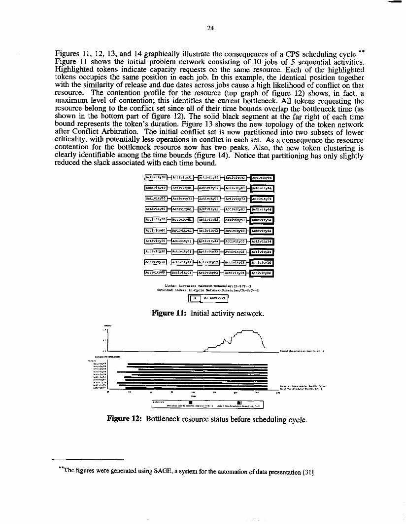
24

Figures 11, 12, 13, and 14 graphically illustrate the consequences of a CPS scheduling cycle.** Figure 11 shows the initial problem network consisting of 10 jobs of 5 sequential activities. Highlighted tokens indicate capacity requests on the same resource. Each of the highlighted tokens occupies the same position in each job. In this example, the identical position together with the similarity of release and due dates across jobs cause a high likelihood of conflict on that resource. The contention profile for the resource (top graph of figure 12) shows, in fact, a maximum level of contention; this identifies the current bottleneck. All tokens requesting the resource belong to the conflict set since all of their time bounds overlap the bottleneck time (as shown in the bottom part of figure 12). The solid black segment at the far right of each time bound represents the token's duration. Figure 13 shows the new topology of the token network after Conflict Arbitration. The initial conflict set is now partitioned into two subsets of lower criticality, with potentially less operations in conflict in each set. As a consequence the resource contention for the bottleneck resource now has two peaks. Also, the new token clustering is clearly identifiable among the time bounds (figure 14). Notice that partitioning has only slightly reduced the slack associated with each time bound.

~ r n r i r w l ~ f i v i ~ ~ i Hlcriulte2 ~ c ~ i ~ i ~ ~ w H A ~ L ~ ~ ~ , . W

*.ririwo Hlcm~w~ H ~ e % ~ i t w Hrcciv'tre H .̂tkviwa

m

-"%,- -.,, .,+., Y-. R-.II,.~I.,I.V ,..,

Figure 12: Bottleneck resource status before scheduling cycle.

'?%e figures were generated using SAGE, a system for the automation of data presentation [3 I ]

25

.. 8 8 ..-... -._.-.- ..... :.., , .".-"-" .-,..... :

Figure 14: New bottleneck rewurce status.

8.2 Experimental evaluation To evaluate the effectiveness of CPS we compared its performance to two other heuristic scheduling methods over a standard scheduling benchmark. The two competing methods rely on the value commitment approach; they are micro-opportunistic search [32] and min-conflict iterative repair [22]. Performance was measured according to the number of problem solved, and the CPU time required.

8.2.1 Experimental design Our experimental analysis was conducted on the Constraint Satisfaction Scheduling benchmark proposed in [32]. The benchmark consists of 6 groups of 10 problems, each problem including 10 jobs and 5 resources. Each job is a linear sequence of 5 activities, each requiring a different resource; in each job, the first activity has a release date and the last a due date. Two features characterize the expected difficulty of each problem group. The first is the spread of release and due dates among jobs; this can be (in order of increasing expected difficulty) wide (w), narrow (n) and null (0). The second is the number of a priory bottlenecks; this can be either 1 or 2.***

For a more detailed description of the benchmark see [32], ***

26

We ran two different configurations of CPS. Backtracking was allowed up to a maximum of 10 times, after which the problem was declared not solved. Each Capacity Analysis step used a total value assignment sample size of N = 2 0 . In both cases the stochastic simulation used forward temporal dispatching as the variable selection strategy; only the value selection rule was different in the two configurations. The (20, ASAP) configuration used a linearly biased value selection rule with highest preference to the earliest time and lowest, 0, to the latest time; the (20, UNIF) configuration used a uniform value selection rule.

We implemented a scheduler, MIN COW, that follows the min-conflict approach. The goal was to evaluate the performance of a scheduler relying almost exclusively on the iterative repair process. For this reason MW CONF displays several differences with respect to the configuration of the Spike scheduling system which was also applied to this benchmark [16]. Both MIN CONF and Spike use a basic cycle that generates an initial total value assignment and applies a process of iterative repair to it. In both cases, if a solution is not found after a fixed number of repairs, the cycle is repeated. MIN CONF and Spike differ greatly with respect to the creation of the initial value assignment. MIN CONF does not make any attempt to generate a “good” initial guess. It generates a total time assignment by executing CPS’s stochastic simulation once. The simulation is configured as forward temporal dispatching with uniform value selection rule. This guarantees satisfaction of job precedences and of release and due dates, but not of capacity constraints. Moreover, the use of a uniform rule biases each operation to occur late in its time bound. Instead, Spike, uses a much more informed initialization method that applies a min-conflict approach. It iteratively selects a variable by using “most-constrained first” and by breaking ties randomly; the variable is then bound to the earliest value among those with the minimum number of conflicts. Both MIN CONF and Spike use similar min-conflict iterative repair cycles. The repair variable is chosen randomly among those currently in conflict. Both methods count capacity conflicts in the same way, but there is a difference in the way job precedence conflicts are counted. MIN CONF counts a single conflict for an activity that violates job precedence constraints with any number of activities. On the other hand, Spike counts one conflict for each job precedence which is violated.

Since the iterative repair phase could cycle indefinitely, MIN CONF limits the number of repairs to 25000; after this threshold the scheduler declares a failure. To evaluate the effect of the length of the repair process we ran MIN CONF in two configurations. In the first, MIN CONF (50, SOO), the initialization occurs every 500 unsuccessful repairs; in the second, MIN C O W (5, SOOO), the limit for each repair phase is 5000 cycles. In both configurations the initialization effort is negligible as compared to the time spent repairing. This bias is consistent with our interest toward isolating the effects of the repair process as much as possible.

The performance of micro-opportunistic search scheduling (MICRO OPP) comes directly from the literature [ 3 2 , 3 3 ] . Micro opportunistic search uses variable and value ordering heuristics based on capacity analysis metrics similar to those of CPS. The performance results refer to two configurations differing on the strategy used to recover from dead ends. The f i t configuration, MICRO OPP CHRON BKTRK, uses chronological backtracking [32]. The second, MICRO OPP INTEL BKTRK, uses a series of intelligent dead end recovery techniques [41 I.

8.2.2 Experimental results Tables 2 and 3 report the comparative performance results. The rows refer to each problem group in the benchmark; for example row w/2 refers to problems with wide spread and two a priori bottlenecks. The last row reports a summary of the performance over the whole benchmark. Since both CPS and MIN CONF have a randomized nature, we estimated their average performance over 5 independent runs. This is not necessary for MICRO OPP since, as we already mentioned in section 8.1, its heuristics are deterministic, although based on probabilistic assumptions.

21

(20,ASAP) 20, UNIF)

Table 2 reports the number of problems solved. The results show that CPS (20, ASAP) and MICRO OPP INTEL BKTRK are the only two techniques that consistently solved all of the problems. The performance differences across the two CPS configurations indicate the importance of the stochastic simulation strategy. For example, The choice of different value selection rules impacts the region of the search space from which sample elements are more likely to be generated. In our case it can be demonstrated that the sample base obtained with a UNIF rule is, in fact, narrower than the one obtained with an ASAP rule. The evaluation of the effect of different sampling strategies on the performance of the scheduler is an important open problem.

Both configurations of MIN CONF performed significantly worse than both CPS and MICRO OPP.**** At first glance this result might seem at odds with the excellent performances displayed on this benchmark by Spike [16]. However, the balance between initialization and repair efforts is very different in the two schedulers. As we mentioned before, since MIN CONF was mainly intended to evaluate the repair process, initialization effort is negligible with respect to repair. Considering the number of time value assignments in each phase, MIN CONF (50, 500) has a 1 to 10 ratio and MIN CONF (5,5000) has a 1 to 100 ratio. Since each initialization assignment is not as “informed” as an assignment during repair, the ratio is even more biased toward repair. Conversely, in Spike initialization and repair efforts are balanced since the same number of value assignments to variables is executed in both phases. Moreover initialization and repair assignments use the same kind of heuristics. An important consequence of this is that, when Spike succeeds, most of the time it does not repair. The dependency of the convergence of the repair process from the choice of a “good” initial solution is still an open problem.

The performance of MIN C O W across problem subsets is worst on the problems with two a priori bottlenecks. When a problem presents several bottlenecks, scheduling algorithms are known to have difficulty in dealing with the complex interactions. These results suggest that the local nature of the conflict measure used in MIN CONF is unable to detect such interactions.

CHRON INTEL (SO. 500) (5? 5000) BKTRK BKTRK

n I CPS I MINCONF 1 MICROOPP I \ 1 I I

w/l W12 dl n12 0/1 w2

10 10 10 10 10 10

10 10 10 9.4 9.4 9

9.8 2.2 7.4 1 4.2 0

9.2 3.2 6.6 1.2 3.4 0.4

10 10 8 9 7 8

10 10 10 10 10 10

I I I I I I

TOT I 60 I 57.8 I 24.6 I 24.0 I 52 I 60

Table 2: Comparative results: number of problems solved.

Table 3 reports average CPU times for a problem run in each subset. The times were obtained by summing up all the processing times for all the problem instances (successful and unsuccessful), dividing by the number of problems, and then averaging over the 5 independent runs. The last row contains average CPU time over the entire benchmark. All the run times refer to implementations in Common Lisp, using CRL as an underlying knowledge representation language. The run times of CPS and MICRO OPP were obtained on a DEC 5000/200

**** In fact, they also are inferior to a number of other heuristic search methods [32].

28

***** workstation.

To ensure a fair comparison, we reduced the actual CPU times for MIN CONF by a factor taking into account the inefficiency of our current implementation. This was done by assuming that the maximum CPU time of any CPS run was equivalent to the time taken to execute the 25000 repairs of a maximum length MIN CONF run; we do not consider the time spent during initialization. These times would require a speed-up of 20 times over our current, inefficient MIN CONF implementation, a factor that we think can be easily achieved by just using more efficient data structures.

A comparison of CPU times serves two main purposes. In first place, the compared techniques are extremely different with respect to several factors. These include: the underlying search method; the computational effort needed to evaluate heuristics; the balance between the time spent in evaluating heuristics and the time spent expanding alternatives. CPU times are the only reasonable way to ensure that each technique is given a comparable “computational allowance” before declaring a failure.. In second place, CPU time indeed depends on the implementation. Implementations are likely to improve with time, and the degree of improvement might differ across techniques. However, if we assume some basic factors as constant, like hardware and programming languages, CPU times are a fair description of the current state of the art of the different techniques.

The comparison of the CPU times shows that CPS is consistently faster than all the other techniques. In particular, comparing the only two techniques that can solve all the problems in the benchmark, CPS (20, ASAP) is about 64% faster on average than MICRO OPP INTEL BKTRK, The experimental results clearly show that CPS outperforms both MIN CONF and MICRO OPP on this benchmark.

I \ I CPS I MINCONP I MICROOPP

wll W/2 dl n12 011 012

68.08 70.67 69.43 72.16 80.20

110.04

152.40 336.17 1 235.08 408.83 333.13 425.10

78.00 82.75

359.25 151.00 462.25 275.00

90.66 94.95

106.22 119.53 134.75 226.56

I AVG 1 78.43 1 92.64 I 298.42 1 315.12 I 234.71 I 128.78

Table 3: Comparative results: CPU time.

9 Conclusions The effectiveness of HSTS has been demonstrated by modeling and solving complex planning and scheduling problems. The principal advantages are the intrinsic modularity of the representation framework, its independence from the problem solving methodology, and the flexibility of the constraint posting and propagation mechanisms. Integrated planner/schedulers have been implemented in domains like space mission scheduling and transportation planning. Although simplified, they have demonstrated the ability to deal effectively with all of the

‘**’%e run times from MICRO OPP CHRON BK7’RK have been obtained from those reported in I321 by assuming the maximum speed-up factor of 2 for moving from a DEC 3100 workstation to a DEC 5ooO/200.

29

important domain constraints. For more classical job-shop constraint satisfaction scheduling problems, the combination of flexibility of the temporal data base and of statistical measures of the search space has yielded promising results. Future research will further address the issue of scalability of the domain models and problem solvers, the extension of constraint language and propagation mechanisms, the development and evaluation of alternative methodologies for capacity analysis, the extension of the statistical search space metrics to integrated planningkcheduling domains, and the assessment of the effectiveness of flexible pldschedule representations during reactive plan execution.

30

Acknowledgments Since the beginning of the project, Stephen Smith has always given valuable support and contributions. Other contributors are Gilad Amiri, Amedeo Cesta, Daniela D' Aloisi, Robert Frederking, and Dhiraj Pathak. Dina Berkowitz, Gregg Podnar, and David Greene helped review a previous draft of this chapter.

31

References Allen, J.F. Maintaining Knowledge about Temporal Intervals. Communications of the ACM 26( 11):832-843, 1983.

Allen, 1. and Koomen, J.A. Planning Using a Temporal World Model. In Proceedings of the 8th International Joint Conference on Artificial Intelligence, pages

Baker, K.R. Iniroduction to Sequencing and Scheduling. John Wiley and Sons, New York, 1974.

Adams, J., Balas, E., Zawack, D. The Shifting Bottleneck Procedure for Job Shop Scheduling. Management Science 34,1988.

Biefeld, E., Cooper, L. Bottleneck Identification Using Process Chronologies. In Proceedings of the 12th Iniernutional Joint Conference on Artijicial Intelligence.

Dean, T.L. and McDermott, D.V. Temporal Data Base Management. Artificial Intelligence 32:l-55, 1987.

Dean, T., Firby, R.J., Miller, D. Hierarchical Planning Involving Deadlines, Travel Time, and Resources. Computational Intelligence 4:381-398, 1988.

Dean, T., Wellman, M. Planning and Control. Morgan Kaufmann, 1991

Dechter, R. and Meiri, I and Pearl, J. Temporal Constraint Networks. Artificial Intelligence 4951-95, May, 1991.

Fikes, R.E., Hart, P.E., Nilsson, N.J. Learning and Executing Generalized Robot Plans. Artijicial Intelligence 3:25 1-288, 1972.

Fox, M.S., Smith, S.F. ISIS: A Knowledge-Based System for Factory Scheduling. Expert Syftems 1(1):25-49, 1984.

Frederking, R.E., Muscettola, N. Temporal Planning for Transportation Planning and Scheduling. In Proceeding of I992 IEEE International Conference on Robotics and Automation (to

741-747. 1983.

1991.

appear). 1992.

5L

Forbus, K.D. Introducing Actions into Qualitative Simulation. In Proceedings of the Eleventh International Joint Conference on Artificial Intelligence,

pages 1273-8. Morgan Kaufmann, 1989.

Hanes, S.H. (editor). The Joint Staff Officer’s Guide. U.S. Government Printing Office, 1988. Publication 1, Armed Forces Staff College.

Haralick, R.M. and Elliot, G.L. Increasing Tree Search Efficiency for Constraint Satisfaction Problems. Artificial Intelligence 14(3):263-3 13, October, 1980.

Johnston, M.J., Minton, S. Analyzing a Heuristic Strategy for Constraint Satisfaction and Scheduling. Intelligent Scheduling. In Fox, M.S. and Zweben, M., Morgan Kaufmann, 1993.

Kalman, R.E. and Falb, P.L. and Arbib, M.A. Topics in Mathematical System &og. McGraw-Hill, 1969.

Vilain, M. and Kautz, €3. and van Beek, P. Constraint Propagation Algorithms for Temporal Reasoning: A Revised Report. Qualitative Reasoning about Physical Systems. Morgan Kaufmann, 1990.

Knoblock, C.A. Automatically Generating Abstractions for Problem Solving. PhD thesis, School of Computer Science, Carnegie Mellon University, 1991.

Lansky, A. Localized Event-bawd Reasoning for Multiagent Domains. Computational Intelligence 4 3 19-34. 1988.

Manna, 2. and Pnueli, A. The Temporal Logic of Reactive and Concurrent Systems. Springer-Verlag, 1991-, 1991.

Minton, S., Johnston, M. D., Philips, A. B., Laird, P. Minimizing Conflicts: a Heuristic Repair Method for Constraint Satisfaction and

Artificial Intelligence 58:361-205, 1992.

Muscettola, N. Planning the Behavior of Dymmical Systems. Technical Report CMU-RT-TR-90-10, The Robotics Institute, Carnegie Mellon

Scheduling Problems.

University, 1990.

33

[24] Muscettola, N., S.F. Smith. A Probabilistic Framework for Resource-Constrained Multi-Agent Planning. In Proceedings of the 10th International Joint Conference on Artificial Intelligence,

pages 1063-1066. Morgan Kaufmann, 1987.

Muscettola, N., Smith, S.F., Cesta, A,, D'Aloisi, D. Coordinating Space Telescope Operations in an Integrated Planning and Scheduling

[25]

Architecture. IEEE Control SystemsMagazine 12(2), 1992.

r301

1311

Muscettola, N. Scheduling by Zterative Partition of Bottleneck Conflicts. Technical Report CMU-RI-TR-92-05, The Robotics Institute, Carnegie Mellon

Muscettola, N. Scheduling by Iterative Partition of Bottleneck Conflicts. In Proceedings of the 9th Conference on Artificial Intelligence for Applications. IEEE

Muscettola, N . An Experimental Analysis of Bottleneck-Centered Opportunistic Scheduling. Technical Report, The Robotics Institute, Carnegie Mellon University, 1993

Ow, P.S., Smith, S.F. Viewing Scheduling as an Opportunistic Problem Solving Process. In R.G. Jeroslow (editor), Annals of Operations Research 12. Baltzer Scientific

Publishing Co., 1988.

Panwalker, S.S., W. Iskander. A Survey of Scheduling Rules. Operations Research 25:45-6 1, 1977.

Roth, S.F., Mattis, J. Automating the Presentation of Information. In Proceedings of the Conference on Artificial Intelligence Applications. IEEE, Miami

Sadeh, N. Look-Ahead Techniques for Micro-Opportunis tic Job Shop Scheduling. Technical Report CMU-CS-91-102, School of Computer Science, Carnegie Mellon

Norman Sadeh, Katia Sycara, and Yalin Xiong. A Comparative Study of Backtracking Techniques for Hard Scheduling Problems. Technical Report, The Robotics Institute, Carnegie Mellon University, 1993

Schrag, R., Boddy, M., Carciofmi, J. Managing Disjunction for Practical Temporal Reasoning. In Proceedings of the Third International Conference on Principles of Knowledge

University, February, 1992.

Computer Society Press, March, 1993.

(foahcoming).

Beach, February, 1991.

University, 1991.

(forthcoming).

Representation and Reasoning. Morgan Kaufmann, KR'92, Cambridge, MA, 1992.

34

Smith, S.F and D.K. Pathak. Balancing Antagonistic Time and Resource Utilization Constraints in Over-Subscribed

Scheduling Problems. In Proceedings 8th IEEE Conference on AI Applications. March, 1992.

Smith, S.F., Ow, P.S., Potvin, J.Y., Muscettola, N., and Matthys, D. An Integrated Framework for Generating and Revising Factory Schedules. Journal of the Operational Research Society 41(6):539-552, 1990.

STScI. Proposal Instructions for the Hubble Space Telescope. Technical Report, Space Telescope Science Institute, 1986.

Currie, K. and Tate, A. 0-plan: the Open Planning Architecture. Artificial Intelligence 52( 1):49-86, 1991.

Vere, S. Planning in Time: Windows and Durations for Activities and Goals. IEEE Tr;?nsactions on Paitern Analysis andMachme Intelligence PAMI-5, 1983.

Wilkins, D.E. Practical Planning. Morgan Kaufrnann, 1988.

Yalin Xiong, Norman Sadeh, and Katia Sycara. Intelligent Backtracking Techniques for Job Shop Scheduling. tn Proceedings of the Third International Conference on Principles of Knowledge

Representation and Reasoning, pages 1423. KR’92, Cambridge, MA, October, 1992.

Zweben, M., Deale, M., Gargan, R. Anytime Rescheduling. In Proceeding of the DARPA Workshop on Innovative Approaches to Planning,

Scheduling and Control. 1990.