Embed Size (px)
Citation preview
Narrow-Band Image Processing for Gastroenterological ExaminationsBruno Miguel Ferreira MendesMestrado em Física MédicaDepartamento de Física
Orientador Ricardo Sousa, Doutor, Instituto de Telecomunicações - UP
Orientador Carla Rosa, Professora Doutora, INESC TEC - UOSE, FCUP


Todas as correções determinadas pelo júri, e só essas, foram efetuadas.
O Presidente do Júri,
Porto, ______/______/_________


To my parents...

"The Devil is in the Details"

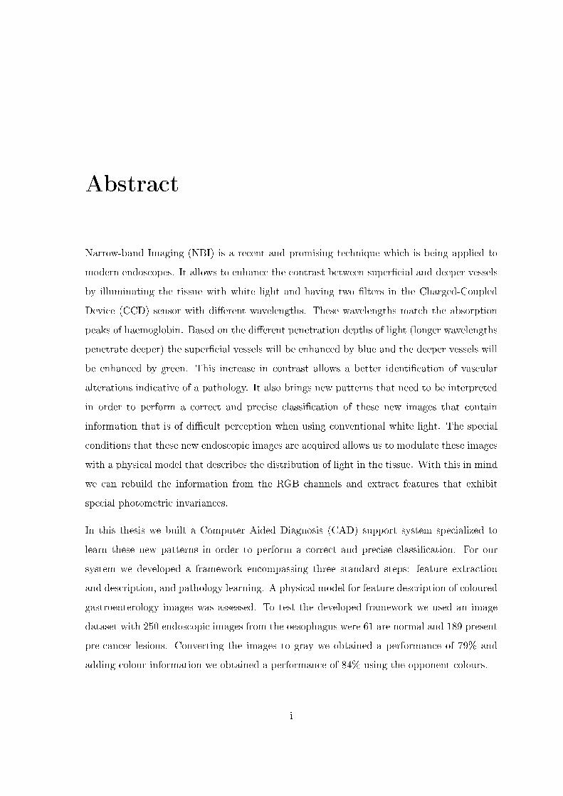
Abstract
Narrow-band Imaging (NBI) is a recent and promising technique which is being applied to
modern endoscopes. It allows to enhance the contrast between super�cial and deeper vessels
by illuminating the tissue with white light and having two �lters in the Charged-Coupled
Device (CCD) sensor with di�erent wavelengths. These wavelengths match the absorption
peaks of haemoglobin. Based on the di�erent penetration depths of light (longer wavelengths
penetrate deeper) the super�cial vessels will be enhanced by blue and the deeper vessels will
be enhanced by green. This increase in contrast allows a better identi�cation of vascular
alterations indicative of a pathology. It also brings new patterns that need to be interpreted
in order to perform a correct and precise classi�cation of these new images that contain
information that is of di�cult perception when using conventional white light. The special
conditions that these new endoscopic images are acquired allows us to modulate these images
with a physical model that describes the distribution of light in the tissue. With this in mind
we can rebuild the information from the RGB channels and extract features that exhibit
special photometric invariances.
In this thesis we built a Computer Aided Diagnosis (CAD) support system specialized to
learn these new patterns in order to perform a correct and precise classi�cation. For our
system we developed a framework encompassing three standard steps: feature extraction
and description, and pathology learning. A physical model for feature description of coloured
gastroenterology images was assessed. To test the developed framework we used an image
dataset with 250 endoscopic images from the oesophagus were 61 are normal and 189 present
pre-cancer lesions. Converting the images to gray we obtained a performance of 79% and
adding colour information we obtained a performance of 84% using the opponent colours.
i

ii
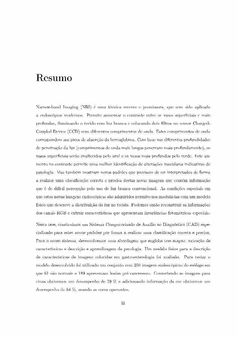
Resumo
Narrow-band Imaging (NBI) é uma técnica recente e promissora, que tem sido aplicada
a endoscópios modernos. Permite aumentar o contraste entre os vasos super�ciais e mais
profundos, iluminando o tecido com luz branca e colocando dois �ltros no sensor Charged-
Coupled Device (CCD) com diferentes comprimentos de onda. Estes comprimentos de onda
correspondem aos picos de absorção da hemoglobina. Com base nas diferentes profundidades
de penetração da luz (comprimentos de onda mais longos penetram mais profundamente), os
vasos super�ciais serão enaltecidos pelo azul e os vasos mais profundos pelo verde. Este au-
mento no contraste permite uma melhor identi�cação de alterações vasculares indicativas de
patologia. Mas também mostram novos padrões que precisam de ser interpretados de forma
a realizar uma classi�cação correta e precisa destas novas imagens que contêm informação
que é de difícil percepção pelo uso de luz branca convencional. As condições especiais em
que estas novas imagens endoscópicas são adquiridos permite-nos modulá-las com um modelo
físico que descreve a distribuição da luz no tecido. Podemos então reconstruir as informações
dos canais RGB e extrair características que apresentam invariâncias fotométricas especiais.
Nesta tese, construímos um Sistema Computorizado de Auxílio ao Diagnóstico (CAD) espe-
cializado para estes novos padrões por forma a realizar uma classi�cação correta e precisa.
Para o nosso sistema, desenvolvemos uma abordagem que engloba três etapas: extração de
características e descrição e aprendizagem da patologia. Um modelo físico para a descrição
de características de imagens coloridas em gastroenterologia foi avaliado. Para testar o
modelo desenvolvido foi utilizado um conjunto com 250 imagens endoscópicas do esófago em
que 61 são normais e 189 apresentam lesões pré-cancerosas. Convertendo as imagens para
cinza obtivemos um desempenho de 79 % e adicionando informação da cor obtivemos um
desempenho de 84 %, usando as cores oponentes.
iii

iv
Acknowledgments
This thesis was a very challenging task. To enter in the world of Pattern Recognition and
Machine Learning was not easy. I must confess that sometimes I felt a little lost trying to
understand some of the terminologies and methods used in this �eld of Image Processing.
I was able to overcome these di�culties thanks to my supervisor Doctor Ricardo Sousa.
Thanks for being always available to answer my questions, for the patience in those moments
I was struggling and making mistakes and for the great support given in this journey.
I also would like to thank to my supervisor Professor Doctor Carla Rosa for the suggestions
and support given in the Physics formulation of this thesis and for providing a working space
at INESC-Porto-UOSE.
A big thanks also to Universidade do Porto (Faculdade de Ciências) and to INESC-Porto.
To my parents, for the understanding and support despite of the di�culties that life brings.
To my brother, that was my travelling comrade and had to put up with me every mornings,
to all my friends for being there when I needed and last but not least, to my girlfriend, for
the patience, love and support in this tough journey of my life.
The work developed in this thesis was �nancially supported by FCT (Portuguese Science
Foundation) grant PTDC/EIA-CCO/109982/2009 (CAGE).
v

vi
Contents
Abstract i
Resumo iii
Acknowledgments v
List of Tables xi
List of Figures xiv
List of Algorithms xv
1 Introduction 1
1.1 Motivation . . . . . . . . . . . . . . . . . . . . . . . . . . . . . . . . . . . . . . 3
1.2 Objectives . . . . . . . . . . . . . . . . . . . . . . . . . . . . . . . . . . . . . . 5
1.3 Thesis Outline . . . . . . . . . . . . . . . . . . . . . . . . . . . . . . . . . . . 6
1.4 Contributions . . . . . . . . . . . . . . . . . . . . . . . . . . . . . . . . . . . . 7
2 Background Knowledge 9
2.1 The Oesophagus . . . . . . . . . . . . . . . . . . . . . . . . . . . . . . . . . . 9
2.2 Grading System . . . . . . . . . . . . . . . . . . . . . . . . . . . . . . . . . . . 11
vii
2.3 The Theory of Narrow-Band Imaging . . . . . . . . . . . . . . . . . . . . . . . 12
2.4 The Dichromatic Re�ection Model . . . . . . . . . . . . . . . . . . . . . . . . 15
3 Invariant Features 19
3.1 Related Work . . . . . . . . . . . . . . . . . . . . . . . . . . . . . . . . . . . . 19
3.2 Scale Invariant Feature Transform . . . . . . . . . . . . . . . . . . . . . . . . 21
3.2.1 The SIFT detector . . . . . . . . . . . . . . . . . . . . . . . . . . . . . 22
3.2.2 The SIFT descriptor . . . . . . . . . . . . . . . . . . . . . . . . . . . . 24
3.2.3 Sampling Strategies . . . . . . . . . . . . . . . . . . . . . . . . . . . . 25
4 Adding Colour Information 27
4.1 Colour Spaces . . . . . . . . . . . . . . . . . . . . . . . . . . . . . . . . . . . . 27
4.2 Photometric Invariant Features . . . . . . . . . . . . . . . . . . . . . . . . . . 31
5 Pathology Recognition 37
5.1 Linearly Separable Binary Classi�cation . . . . . . . . . . . . . . . . . . . . . 37
5.2 Binary Classi�cation for Data not Fully Linearly Separable . . . . . . . . . . 41
5.3 Non-linear Support Vector Machine . . . . . . . . . . . . . . . . . . . . . . . . 42
6 Experimental Study 43
6.1 Image dataset . . . . . . . . . . . . . . . . . . . . . . . . . . . . . . . . . . . . 43
6.2 Methodology . . . . . . . . . . . . . . . . . . . . . . . . . . . . . . . . . . . . 44
6.2.1 Extracting colour features . . . . . . . . . . . . . . . . . . . . . . . . . 45
6.2.2 Building the vocabulary . . . . . . . . . . . . . . . . . . . . . . . . . . 47
6.2.3 Training the classi�er . . . . . . . . . . . . . . . . . . . . . . . . . . . 47
viii
6.3 Validating the parameters . . . . . . . . . . . . . . . . . . . . . . . . . . . . . 48
6.4 Assessing the Classi�er Performance . . . . . . . . . . . . . . . . . . . . . . . 49
7 Results and Discussion 51
8 Conclusions and Future Works 59
A Abbreviations 61
B Published Article at RecPad2013 63
References 66
ix

x
List of Tables
1.1 Classi�cation of Oesophageal cancer according to its extension. . . . . . . . . 4
6.1 Grouping the images for a binary classi�cation system. . . . . . . . . . . . . . 44
7.1 Mean errors obtained for the Linear, Intersection and χ2 kernels. . . . . . . . 51
7.2 Mean Average Precision (MAP) vs # of visual words vs ∆t. . . . . . . . . . . 52
7.3 The results of the ten simulations for each descriptor set. . . . . . . . . . . . . 52
7.4 The impact of colour on the classi�er performance. . . . . . . . . . . . . . . . 53
7.5 A typical confusion matrix for a binary problem. . . . . . . . . . . . . . . . . 54
7.6 Confusion matrices for each set of descriptors in average for the 10 simulations. 55
7.7 Evaluation of several parameters for each set of descriptors. . . . . . . . . . . 56
7.8 Binary classi�er performance assessment . . . . . . . . . . . . . . . . . . . . . 57
xi

xii
List of Figures
1.1 E�ect of NBI (Figure from Muto et al. (2009))1. . . . . . . . . . . . . . . . . 2
1.2 5-year survival rate for some parts of the gastrointestinal tract3. . . . . . . . . 3
1.3 Distribution of oesaphageal cancer according to its extension3. . . . . . . . . . 4
2.1 The layers in the oesophagus. . . . . . . . . . . . . . . . . . . . . . . . . . . . 10
2.2 Sample images of our dataset following Singh's Grading System. . . . . . . . . 11
2.3 Absorption spectra of haemoglobin in blood (Figure from Niemz (2007)). . . . 12
2.4 Absorption lengths in NBI and the enhancement of the capillaries (Figure from
Bryan et al. (2008)). . . . . . . . . . . . . . . . . . . . . . . . . . . . . . . . . 13
2.5 Re�ection of light from an inhomogeneous material (Figure from Shafer (1985)). 16
2.6 Photometric Angles (Figure from Shafer (1985)). . . . . . . . . . . . . . . . . 17
3.1 The SIFT method (Adopted from (Vedaldi & Fulkerson, 2008). . . . . . . . . 22
3.2 The computation of the DoG. (Figure from Lowe (2004)). . . . . . . . . . . . 23
3.3 The SIFT descriptor. . . . . . . . . . . . . . . . . . . . . . . . . . . . . . . . . 24
3.4 Dense sampling strategy. . . . . . . . . . . . . . . . . . . . . . . . . . . . . . . 25
4.1 (a) The addictiveness of the RGB system. (b) The RGB cube. (c) The
chromaticity triangle. . . . . . . . . . . . . . . . . . . . . . . . . . . . . . . . . 28
xiii
4.2 The opponent process theory. . . . . . . . . . . . . . . . . . . . . . . . . . . . 29
4.3 (a) Shadow-shading direction. (b) Specular direction. (c) Hue direction.
(Adopted from Van De Weijer et al. (2005)). . . . . . . . . . . . . . . . . . . . 30
4.4 Gray-scale image and the r and g channels. . . . . . . . . . . . . . . . . . . . 32
4.5 The ratio of the channels. . . . . . . . . . . . . . . . . . . . . . . . . . . . . . 33
4.6 The logarithm of the ratio of the channels. . . . . . . . . . . . . . . . . . . . . 33
4.7 The opponent colour channels. . . . . . . . . . . . . . . . . . . . . . . . . . . 34
4.8 The Hue and the chromatic opponent colours. . . . . . . . . . . . . . . . . . . 35
5.1 Linear discriminant function in a two dimensional feature space (Adopted from
Bishop & Nasrabadi (2006)). . . . . . . . . . . . . . . . . . . . . . . . . . . . 38
5.2 Decision plane through two linearly separable classes. . . . . . . . . . . . . . . 40
5.3 Decision plane through two non-linearly separable classes . . . . . . . . . . . 41
6.1 Experimental Setup . . . . . . . . . . . . . . . . . . . . . . . . . . . . . . . . 44
6.2 Multi-scale DSIFT extraction. . . . . . . . . . . . . . . . . . . . . . . . . . . . 45
6.3 The geometry of the DSIFT approach. . . . . . . . . . . . . . . . . . . . . . . 45
xiv
List of Algorithms
6.1 Method to extract multi-scale features from the images . . . . . . . . . . . . . 46
6.2 Calculating the visual terms with k-means. . . . . . . . . . . . . . . . . . . . 48
6.3 Building the vocabulary for each image . . . . . . . . . . . . . . . . . . . . . . 48
6.4 3-fold Cross-Validation . . . . . . . . . . . . . . . . . . . . . . . . . . . . . . . 49
6.5 The Classi�er . . . . . . . . . . . . . . . . . . . . . . . . . . . . . . . . . . . . 50
xv

Chapter 1
Introduction
"A picture is worth more than a thousand words". This old adage referring to the amount
of information an image can convey has been around us for ages. Of course its origins had
nothing to do with medical images, but its essence is totally applied. With the advances
in science and technology, we are nowadays capable to obtain better quality images of the
human body. This has brought major advantages in diagnosing, monitoring or treating a
disease. In Medical Imaging it is common to use either invisible light, as in an X-Ray exam
or visible light like in an endoscopic procedure. In both the interpretation of these images is
drawn by the physicians experience and expertise adding always a subjective element to the
analysis. With the introduction of computers in Medical Imaging the subjectiveness in the
analysis has diminished. It was in this context that the Computer Aided Diagnosis (CAD)
support systems appeared, to help in the decision and classi�cation process. The advantage
of having a system insensitive to fatigue or distraction is a major plus because we are also
withdrawing the ambiguity and subjectiveness of human analysis. The �rst CAD systems
appeared initially connected to endoscopic images (Liedlgruber & Uhl, 2011).
Endoscopy is a technique widely used in modern medicine to observe the inner cavities
of the human body. It makes use of an endoscope which is basically a �exible tube that
consists of a bundle of optical �bres. The endoscope has evolved a lot since the �rst rigid
endoscope introduced in a demonstration of gastroscopy by Adolph Kussmaul in 1868. The
modern ones allow to view a real time image on a monitor. They are called video endoscopes
1
2 CHAPTER 1. INTRODUCTION
and use a Charged-Coupled Device (CCD) for image generation. A CCD chip is an array of
individual photo cells (or pixels) that receive photons re�ected from a surface and produce
electrons proportionally to the amount of light received. This information is then stored in
memory chips and processed in a monitor (Muto et al., 2009).
A recent technique in endoscopy consists in using only certain wavelengths of visible light
by placing a �lter in front of the light source therefore narrowing the bandwidth of the light
output. This technique is called Narrow-band Imaging (NBI) and is a very promising tool
in the diagnosis of gastrointestinal diseases. The NBI system uses two speci�c wavelengths,
415 nm and 540 nm that match the absorption peaks of haemoglobin. NBI can be used
in a RGB Sequential System which consists of inserting a RGB rotary �lter in front of the
light source but only the green and blue �lter are activated. Another approach is to place
colour �lters in each pixel of the CCD chip. In both systems a Xenon lamp is used as a light
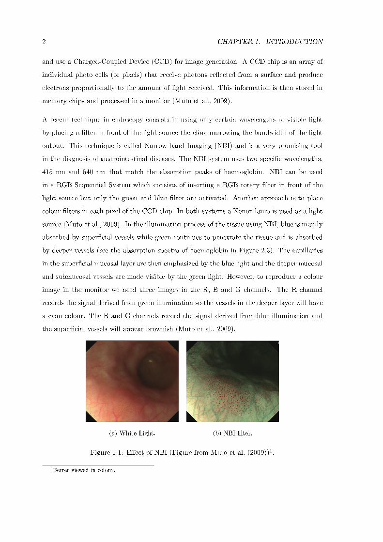
source (Muto et al., 2009). In the illumination process of the tissue using NBI, blue is mainly
absorbed by super�cial vessels while green continues to penetrate the tissue and is absorbed
by deeper vessels (see the absorption spectra of haemoglobin in Figure 2.3). The capillaries
in the super�cial mucosal layer are then emphasized by the blue light and the deeper mucosal
and submucosal vessels are made visible by the green light. However, to reproduce a colour
image in the monitor we need three images in the R, B and G channels. The R channel
records the signal derived from green illumination so the vessels in the deeper layer will have
a cyan colour. The B and G channels record the signal derived from blue illumination and
the super�cial vessels will appear brownish (Muto et al., 2009).
(a) White Light. (b) NBI �lter.
Figure 1.1: E�ect of NBI (Figure from Muto et al. (2009))1.
1Better viewed in colour.
1.1. MOTIVATION 3
Figure 1.1 shows how a Human sees a tissue without (left �gure) and with NBI (right �gure).
In the normal image vascular patterns are di�cult to visualize. The surface of the oesophagus
appears smooth. Depending of the NBI technology employed, we are able to identify some
polyps and a vascular pattern at the surface with a brownish colour. Deeper vessels are
also emphasized appearing with a slight cyan colour. Despite of the technology, NBI is
a very promising tool in the early diagnosis of gastroenterological pathologies decreasing
the examination time, reducing unnecessary biopsies and increasing the accuracy of such
examinations (Muto et al., 2009).
1.1 Motivation
In the twentieth century the average life expectancy from birth in Portugal has increased
and in 2011 was of about 80 years. The main causes of death are cardiovascular diseases and
cancer2. Although the e�orts for prevention and early detection have been made, cancer is
still an issue in public health. According to Registo Oncológico Regional do Norte (RORENO)
the total number of new patients observed at Instituto Português de Oncologia do Porto
Francisco Gentil (IPO-Porto) in 2010 was of 102413. From those 7050 were malignant.
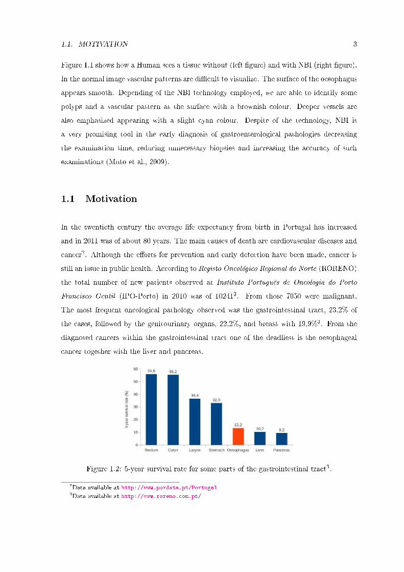
The most frequent oncological pathology observed was the gastrointestinal tract, 23,2% of
the cases, followed by the genitourinary organs, 22,2%, and breast with 19,9%3. From the
diagnosed cancers within the gastrointestinal tract one of the deadliest is the oesophageal
cancer together with the liver and pancreas.
Figure 1.2: 5-year survival rate for some parts of the gastrointestinal tract3.
2Data available at http://www.pordata.pt/Portugal3Data available at http://www.roreno.com.pt/
4 CHAPTER 1. INTRODUCTION
Oesophageal cancer is classi�ed mainly in two groups: squamous cell carcinoma and adeno-
carcinoma. According to RORENO the squamous cell carcinoma represents 101 of the 121
diagnosed cases and adenocarcinoma represents 14 cases and other tumours with 6 cases3.
The disease can also be classi�ed in terms of its extension in �ve groups4.
In Situ malignant tumour that has not penetrated the basement membrane not
extended beyond the epithelial tissue
Localized invasive malignant tumour con�ned to the organ of origin
Regional malignant tumour that has extended beyond the limits of the organ of
origin directly into surrounding organs and tissues or evolved through
the lymphatic system or both
Distant malignant tumour that has spread to parts of the body remote from the
primary tumour either by direct extension or by metastasis
Not Recorded insu�cient information to assign a stage
Table 1.1: Classi�cation of Oesophageal cancer according to its extension.
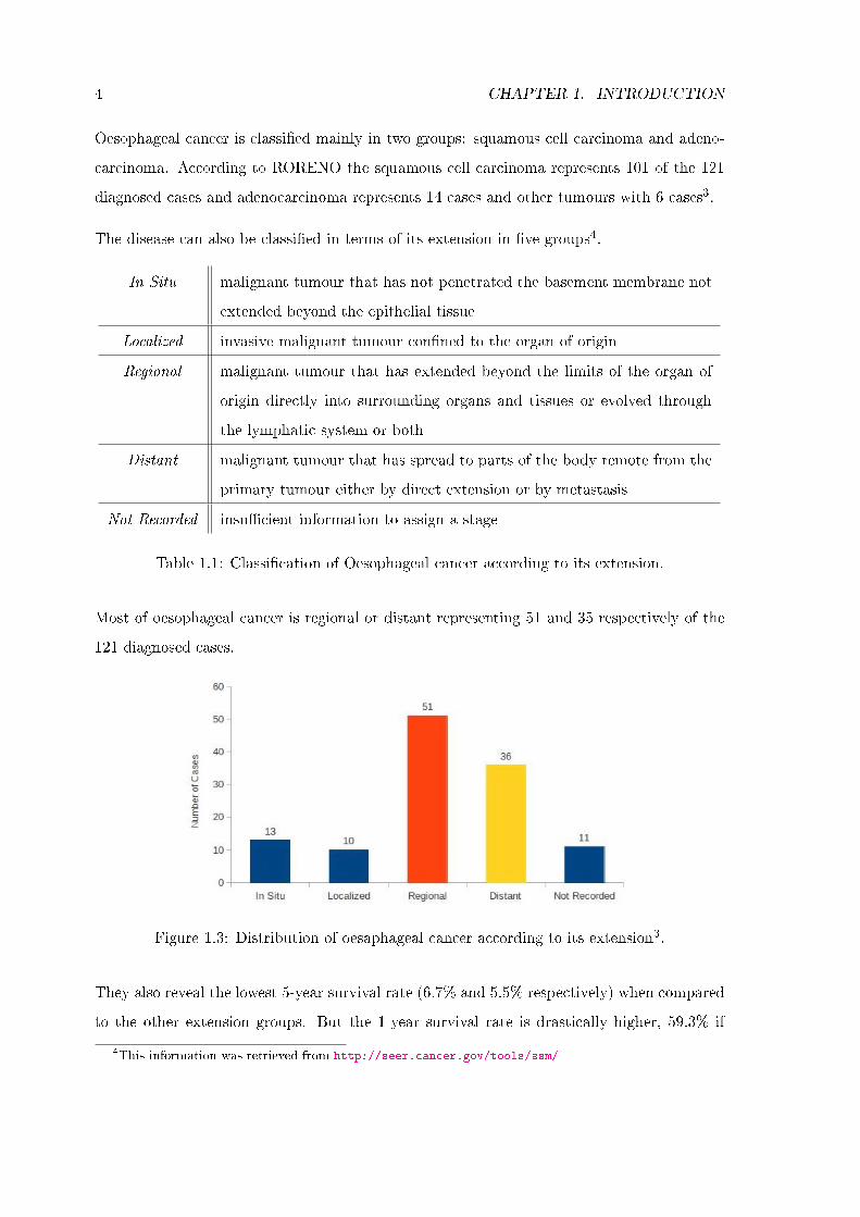
Most of oesophageal cancer is regional or distant representing 51 and 35 respectively of the
121 diagnosed cases.
Figure 1.3: Distribution of oesaphageal cancer according to its extension3.
They also reveal the lowest 5-year survival rate (6.7% and 5.5% respectively) when compared
to the other extension groups. But the 1-year survival rate is drastically higher, 59.3% if
4This information was retrieved from http://seer.cancer.gov/tools/ssm/
1.2. OBJECTIVES 5
regional, and 30.3% if metastatic3.
It is thus crucial to detect oesophageal cancer, or any other type of cancer per say, in its early
stages. In this context the NBI technique provides a valuable tool, emphasizing the mucosal
microvasculature allowing the identi�cation of vascular alterations indicative of a pathology.
The use of two well de�ned wavelengths allows to visualize structures that were masked by
conventional light. The possibility of observing structures lying deeper in the mucosa and the
increase in contrast of super�cial patterns that may be indicative of a pathology supply a very
important visual tool for a correct early diagnosis. A CAD system capable of an accurate
early detection is crucial in order to increase the odds for survival. Unfortunately, according
to a study performed by Liedlgruber & Uhl (2011) the number of CAD related publications
on the oesophagus is small when compared to other parts of the gastrointestinal tract. This
number is even smaller when considering the new images acquired by NBI endoscopy.
1.2 Objectives
The increasing need of better decisions on the recognition of a pathology leads to the
development of more accurate CAD system. In this context with this thesis we propose
to study existing methods in the image processing �eld and apply them to NBI images. The
special characteristics in the acquisition of NBI images leads to the need of developing new
methods to describe these images in order to attain an improved classi�cation performance.
Rich information is therefore necessary and due to the fact that NBI is a quite recent
technology, the lack of works done in this area is a big drawback.
In this thesis we study state of the art image processing techniques to describe gastroen-
terological images and develop a robust framework to classify these new images. Although,
Computer Vision community usually use local or global analysis techniques for the processing
and description of information, in gastroenterological images most research has been focused
on global analysis techniques (a more detailed description will be given in Section 3.2). In
this work we explore the usage of local image information.
The impact in classi�cation of the independent information from the RGB channels is
also studied by considering some physical principles in the image acquisition process. The
6 CHAPTER 1. INTRODUCTION
new patterns revealed by NBI and the high mortality of oesophageal cancer demands the
development of a CAD system specialized in the determination of patterns that may be
indicative of an evolution to cancer.
1.3 Thesis Outline
In Chapter 1 the NBI was introduced. The arising of NBI was natural in the sense of looking
for ways of increasing the contrast between structures to allow a better early diagnostic. Some
statistical data from RORENO is presented in order to motivate the need of the introduction
of a CAD system appropriated to these new images.
In Chapter 2 we begin by introducing the physiological and anatomical properties of the
oesophagus for a better understanding of the patterns found in the mucosa that will be
characteristic of a possible pathology. All the images were in a pre-cancer stage and the
used grading system is also presented. The scienti�c basis behind NBI is analysed and the
main physical principles of the interaction of light with matter are introduced for a better
understanding of the characteristics of the images and �nally the Dichromatic Re�ection
Model are also presented.
Chapter 3 is dedicated to the process of extracting features from the images and we begin
by presenting a literature review on this subject. In his thesis we propose to perform this
task with local descriptors. We also present the sampling strategy that was used to extract
rich information from the images.
Chapter 4 is dedicated to the presentation of some photometric invariants derived from the
valid assumption of the Dichromatic Re�ection Model. These photometric invariants are
derived from the RGB colour model and we also derive the expressions for the opponent
colour system as well as the respective invariants.
Chapter 5 is dedicated to the presentation of the learning method used in this thesis were
we present some basic principles of the Support Vector Machine. In Chapter 6 we begin by
presenting the separation of the images into two classes thus reducing to a binary classi�cation
problem. The main idea is to separate normal from abnormal cases. The used methodology
to extract features, to build a vocabulary that will describe each image and the determination
1.4. CONTRIBUTIONS 7
of a proper set of descriptors to build our classi�er, is also presented.
Next, in Chapter 7 we present the obtained results and we perform the discussion of the
same and �nally, in Chapter 8 we present the �nal conclusions of the developed work and
future developments in the sense of improving the obtained results.
1.4 Contributions
The main contributions of the work presented in this thesis towards the recognition of pre-
cancer lesions in gastroenterological images were the following:
1. Development of a framework for the representation of the images;
2. Analysis and assessment of the e�ectiveness of local descriptors;
3. Improvement of the recognition of pathologies through the addition of colour informa-
tion based on physical models;
4. The developed work in this thesis was published at RecPad 2013 5.
5http://soma.isr.ist.utl.pt/recpad/

8 CHAPTER 1. INTRODUCTION
Chapter 2
Background Knowledge
In this Chapter we begin to review the morphological and physiological characteristics of the
oesophagus. In the �rst Section the structure of the oesophagus is described as well as the
functionality of the di�erent layers. It is also referred the main types of cancer found. Next,
the visual patterns of the oesophagus that indicate a possible pathology are explained based
on a simpli�ed grading system of mucosal morphology against histology. We introduce the
scienti�c basis behind NBI giving special focus on the absorption phenomenon that occurs
due to the presence of haemoglobin in the capillaries. This absorption will have an impact on
the formed image and thus it is critical to understand. We also review some basic physical
principles mainly the ones that allow the understanding and in�uence the colours obtained
from the image. Colour is in fact the crucial basis of this work and a more detailed description
of the physical phenomenons that a�ect colour are referred as well as a physical model from
whom all the images will be based. This model will be used in later chapters to build
alternative colour spaces and derive photometric invariants.
2.1 The Oesophagus
The oesophagus is a �attened muscular tube of 18 to 26 cm in length. Microscopically, the
oesophageal wall is composed of 4 layers: internal mucosa, submucosa, muscularis propria
and adventitia. Unlike the remainder of the gastrointestinal tract, the oesophagus has no
serosa. This fact allows tumours to spread more easily and make them harder to treat
9
10 CHAPTER 2. BACKGROUND KNOWLEDGE
surgically and also makes luminal disruptions more challenging to repair (Jobe et al., 2009).
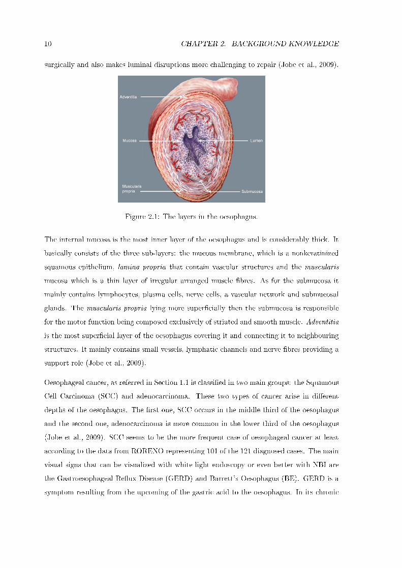
Figure 2.1: The layers in the oesophagus.
The internal mucosa is the most inner layer of the oesophagus and is considerably thick. It
basically consists of the three sub-layers: the mucous membrane, which is a nonkeratinized
squamous epithelium, lamina propria that contain vascular structures and the muscularis
mucosa which is a thin layer of irregular arranged muscle �bres. As for the submucosa it
mainly contains lymphocytes, plasma cells, nerve cells, a vascular network and submucosal
glands. The muscularis propria lying more super�cially then the submucosa is responsible
for the motor function being composed exclusively of striated and smooth muscle. Adventitia
is the most super�cial layer of the oesophagus covering it and connecting it to neighbouring
structures. It mainly contains small vessels, lymphatic channels and nerve �bres providing a
support role (Jobe et al., 2009).
Oesophageal cancer, as referred in Section 1.1 is classi�ed in two main groups: the Squamous
Cell Carcinoma (SCC) and adenocarcinoma. These two types of cancer arise in di�erent
depths of the oesophagus. The �rst one, SCC occurs in the middle third of the oesophagus
and the second one, adenocarcinoma is more common in the lower third of the oesophagus
(Jobe et al., 2009). SCC seems to be the more frequent case of oesophageal cancer at least
according to the data from RORENO representing 101 of the 121 diagnosed cases. The main
visual signs that can be visualized with white light endoscopy or even better with NBI are
the Gastroesophageal Re�ux Disease (GERD) and Barrett's Oesophagus (BE). GERD is a
symptom resulting from the upcoming of the gastric acid to the oesophagus. In its chronic
2.2. GRADING SYSTEM 11
stage it is more likely to originate BE because repeated mucosal injury is thought to stimulate
the progression of intestinal metaplasia. BE is de�ned as the replacement, or metaplasia,
of the normal oesophageal squamous mucosa with a columnar epithelium containing goblet
cells. It is the most important risk factor for oesophageal adenocarcinoma (Muto et al.,
2009).
2.2 Grading System
BE is one of the main indicators of a possible pathology in the oesophagus. In Singh
et al. (2008) it was studied and validated a simpli�ed grading system of the several patterns
observed in BE. The system is based on the regularity of the patterns of the pits present in
the mucosa as well as the patterns observed for the capillaries. The proposed system analyses
images in a pre-cancer stage and classi�es them into four distinct classes. As the mucosa
starts to evolve into cancer it's surface becomes smoother, this is, the regular patterns start
fading away. With their study they concluded that the patterns could be divided into four
groups:
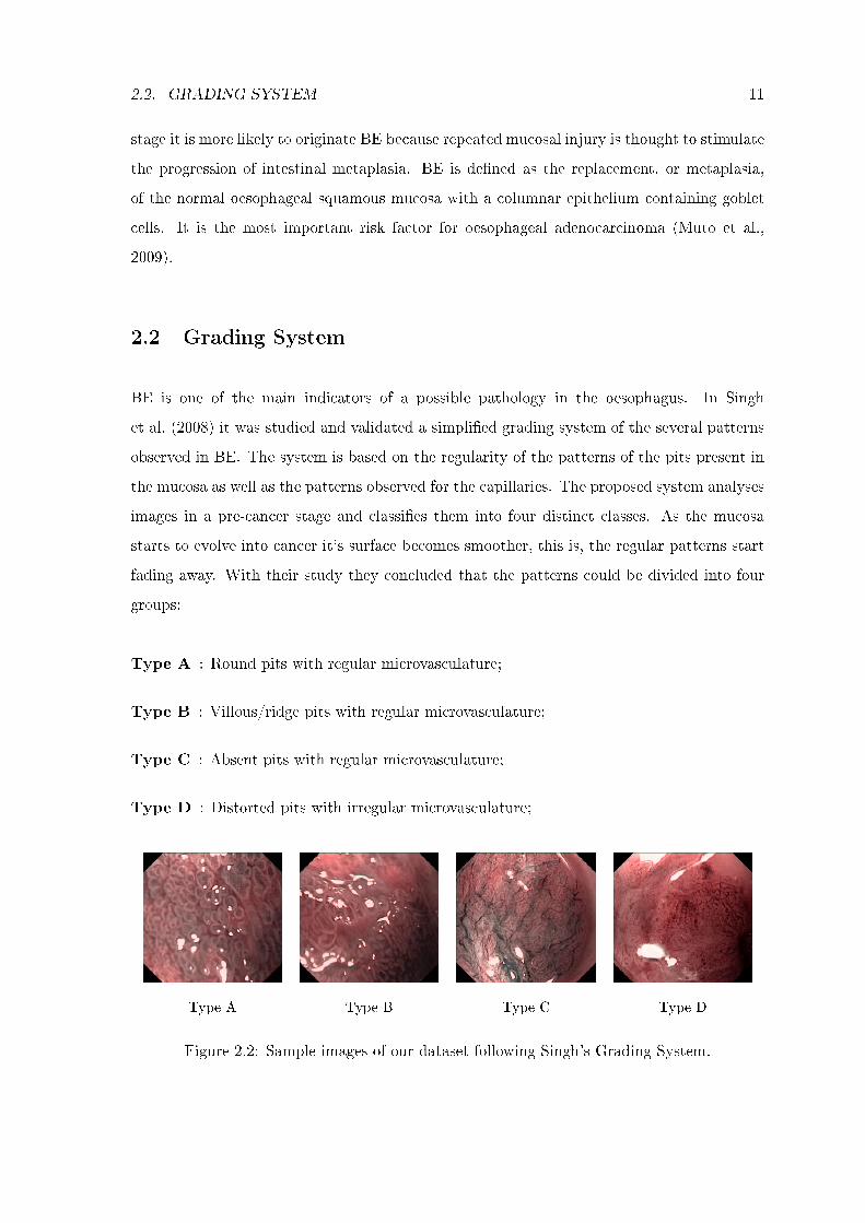
Type A : Round pits with regular microvasculature;
Type B : Villous/ridge pits with regular microvasculature;
Type C : Absent pits with regular microvasculature;
Type D : Distorted pits with irregular microvasculature;
Type A Type B Type C Type D
Figure 2.2: Sample images of our dataset following Singh's Grading System.
12 CHAPTER 2. BACKGROUND KNOWLEDGE
Type A images are normal and type B images are considered with low metaplasia. As for
type C images the absent pits suggest a low dysplasia and type D are in a pre-cancer stage,
high dysplasia. This simpli�ed grading system was the base for this thesis to perform the
separation of the images into the corresponding classes. They were previously classi�ed by a
cohort of experts and validated by histology.
2.3 The Theory of Narrow-Band Imaging
In the NBI technique the selection of two wavelengths that match the absorption peaks of
haemoglobin will cause a maximum absorption of blue and green in di�erent layers of the
mucosa. Absorption occurs because part of the energy of the incident light is converted into
heat through the vibrations of the molecules in the absorbing material. It is described by
Lambert-Beer Law:
I(z) = I0 exp(−µaz) (2.1)
where I(z) is the intensity of light after a path z along the tissue with µa absorption
coe�cient. I0 is the incident intensity. One can de�ne the absorption length L as the
inverse of the absorption coe�cient: L = 1µa. This quantity measures the distance z in which
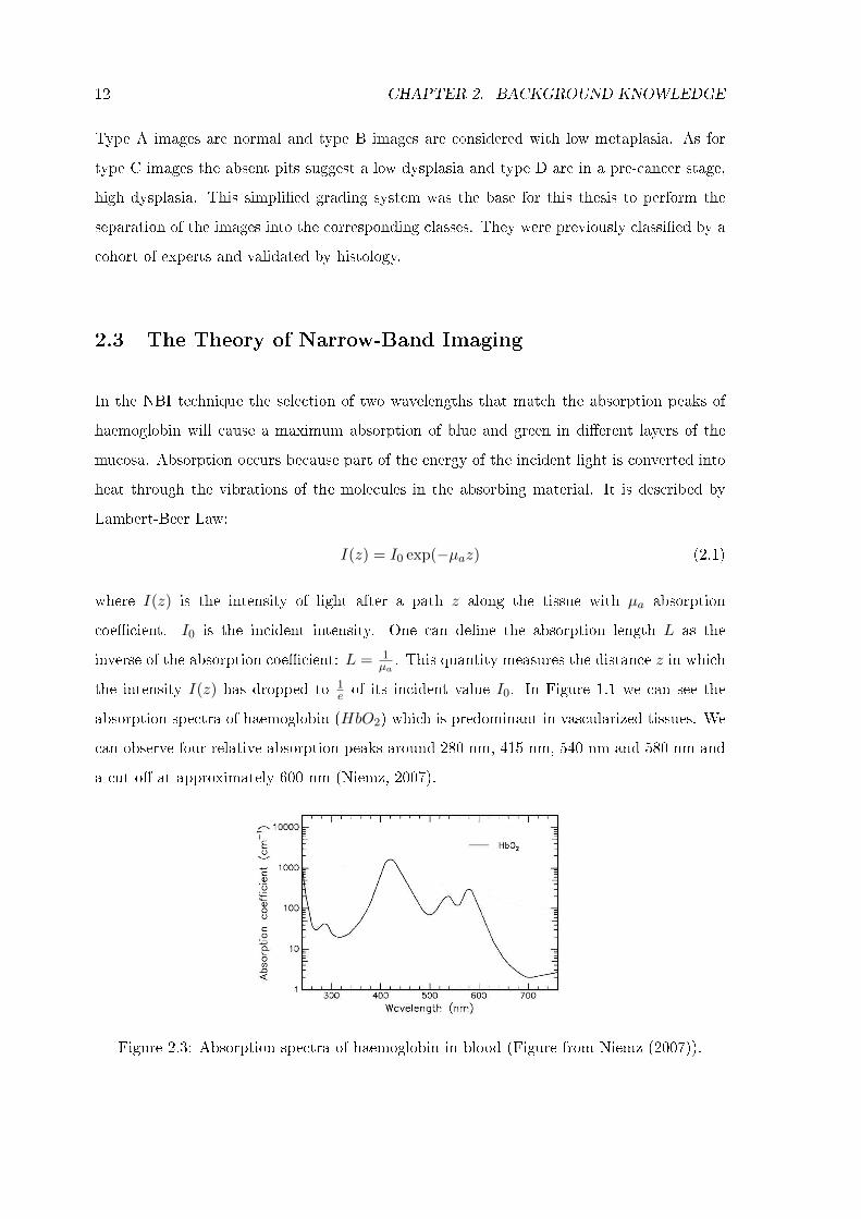
the intensity I(z) has dropped to 1e of its incident value I0. In Figure 1.1 we can see the
absorption spectra of haemoglobin (HbO2) which is predominant in vascularized tissues. We
can observe four relative absorption peaks around 280 nm, 415 nm, 540 nm and 580 nm and
a cut-o� at approximately 600 nm (Niemz, 2007).
Figure 2.3: Absorption spectra of haemoglobin in blood (Figure from Niemz (2007)).
2.3. THE THEORY OF NARROW-BAND IMAGING 13
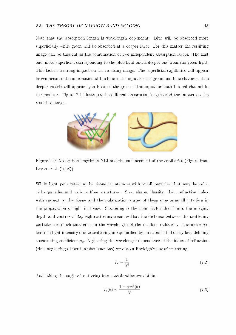
Note that the absorption length is wavelength dependent. Blue will be absorbed more
super�cially while green will be absorbed at a deeper layer. For this matter the resulting
image can be thought as the combination of two independent absorption layers. The �rst
one, more super�cial corresponding to the blue light and a deeper one from the green light.
This fact as a strong impact on the resulting image. The super�cial capillaries will appear
brown because the information of the blue is the input for the grenn and blue channels. The
deeper vessels will appear cyan because the green is the input for both the red channel in
the monitor. Figure 2.4 illustrates the di�erent absorption lengths and the impact on the
resulting image.
Figure 2.4: Absorption lengths in NBI and the enhancement of the capillaries (Figure from
Bryan et al. (2008)).
While light penetrates in the tissue it interacts with small particles that may be cells,
cell organelles and various �bre structures. Size, shape, density, their refractive index
with respect to the tissue and the polarization states of these structures all interfere in
the propagation of light in tissue. Scattering is the main factor that limits the imaging
depth and contrast. Rayleigh scattering assumes that the distance between the scattering
particles are much smaller than the wavelength of the incident radiation. The measured
losses in light intensity due to scattering are quanti�ed by an exponential decay law, de�ning
a scattering coe�cient µs. Neglecting the wavelength dependence of the index of refraction
(thus neglecting dispersion phenomenons) we obtain Rayleigh's law of scattering:
Is ∼1
λ4(2.2)
And taking the angle of scattering into consideration we obtain:
Is(θ) ∼1 + cos2(θ)
λ4(2.3)
14 CHAPTER 2. BACKGROUND KNOWLEDGE
If the spacing between the particles is comparable to the wavelength of the incident light,
as is in blood cells (Niemz, 2007), another theory must be used: Mie scattering. The main
di�erence to Rayleigh's scattering is the dependence on wavelength (∼ λ−x with 0.4 ≤x ≤ 0.5). But the probability of a photon to be scattered in a certain direction must be
taken into consideration. For this matter Henyey�Greenstein proposed the following phase
or probability function:
p(θ) =1− g2
(1 + g2 − 2g cos θ)32
(2.4)
where g represents the coe�cient of anisotropy and has the values 1 or -1, forward and
backward scattering respectively. If g = 0 isotropic scattering occurs. Typical values for g
range from 0.7 to 0.99 for biological tissues and the corresponding scattering angles are 8o
and 45o (Niemz, 2007).
Most biological tissues are turbid and therefore both scattering and absorption will occur.
The mucosa is no exception. For such media one must then de�ne a total attenuation
coe�cient as:
µt = µa + µs (2.5)
thus considering the contributions of scattering (µs) and absorption (µa). One can also de�ne
the mean free optical path of the photons through the mucosa as:
Lt =1
µt(2.6)
In order to have a better idea if a medium is mostly absorbing or scattering, and thus the
attenuation of light is mostly due to absorption or scattering, it is usually de�ned another
parameter, the optical albedo a, given by:
a =µsµt
(2.7)
If a = 0, attenuation is mostly due to absorption, if a = 1 attenuation is mostly due to
scattering and if a = 12 both occur.
In the literature it is common to work with the reduced scattering coe�cient, de�ned as:
µ′s = µs(1− g) (2.8)
Another useful parameter is the optical penetration depth, de�ned as:
d =
∫ s
0µtds
′(2.9)
2.4. THE DICHROMATIC REFLECTION MODEL 15
where ds′is an in�nitesimal segment of the optical path and s is the total length (Niemz,
2007). These de�nitions are very useful for an experimental determination, using for example,
the inverse adding-doubling method. This was performed by Bashkatov et al. (2005). They
determined some optical properties of human skin, subcutaneous adipose tissue and human
mucosa for a wavelength window of 400 nm to 2000 nm. Borrowing the data related to the
human mucosa from their work we observe that the absorption coe�cient of the human
mucosa presents two peaks at approximately 415 nm and 540 nm due to the presence of
haemoglobin in the oxygenated form in the super�cial vessel of the mucosa. The reduced
scattering spectra actually reveals that for the used wavelengths the mucosa is a quite
scattering tissue and presents an anomalous behaviour near the absorption peaks. This
is due to an anomalous light dispersion phenomenon. It is also observed that the penetration
depth of light at the referred wavelengths is very super�cial.
If we illuminate the tissue with white light some of the vascular structures are not visible
neither are other patterns that maybe indicative of a tissue lesion. But narrowing the band
of the light output will reduce scattering e�ects and increase the image de�nition and with
the absorption phenomenon the contrast between super�cial and deeper vessels is achieved
providing a high quality tool for a better diagnosis.
2.4 The Dichromatic Re�ection Model
When a light ray hits a surface of a material part of it will be re�ected and the remaining will
penetrate throw the tissue. While light penetrates in the tissue it can be scattered, absorbed
or in a more realistic case, a little bit of both. If we consider the angle of incidence as being
θi and the angle of re�ection as θr with respect to the normal of the incidence plane, we
have θi = θr. This is the �rst part of the Law of Re�ection. The second part states that the
incident ray, the perpendicular of the surface and re�ected ray all lie in a plane called the
plane of incidence. Ignoring polarization we can obtain the re�ectivity or re�ectance given
by for normal incidence:
R = r2 =
(n0 − n1n0 + n1
)2
(2.10)
where n0 and n1 are the refractive indices of the incidence and transmission media and
they are wavelength dependent, so R will vary along the spectrum. If a re�ecting surface
16 CHAPTER 2. BACKGROUND KNOWLEDGE
is smooth, that is, the irregularities, are small compared to the wavelength, the light re-
emitted by the millions of atoms will combine to form a well de�ned beam in a process called
specular re�ection. On the other hand if the surface is rough compared to the wavelength
the emerging rays will have di�erent directions constituting what is called di�use re�ection
(Hecht, 1998).
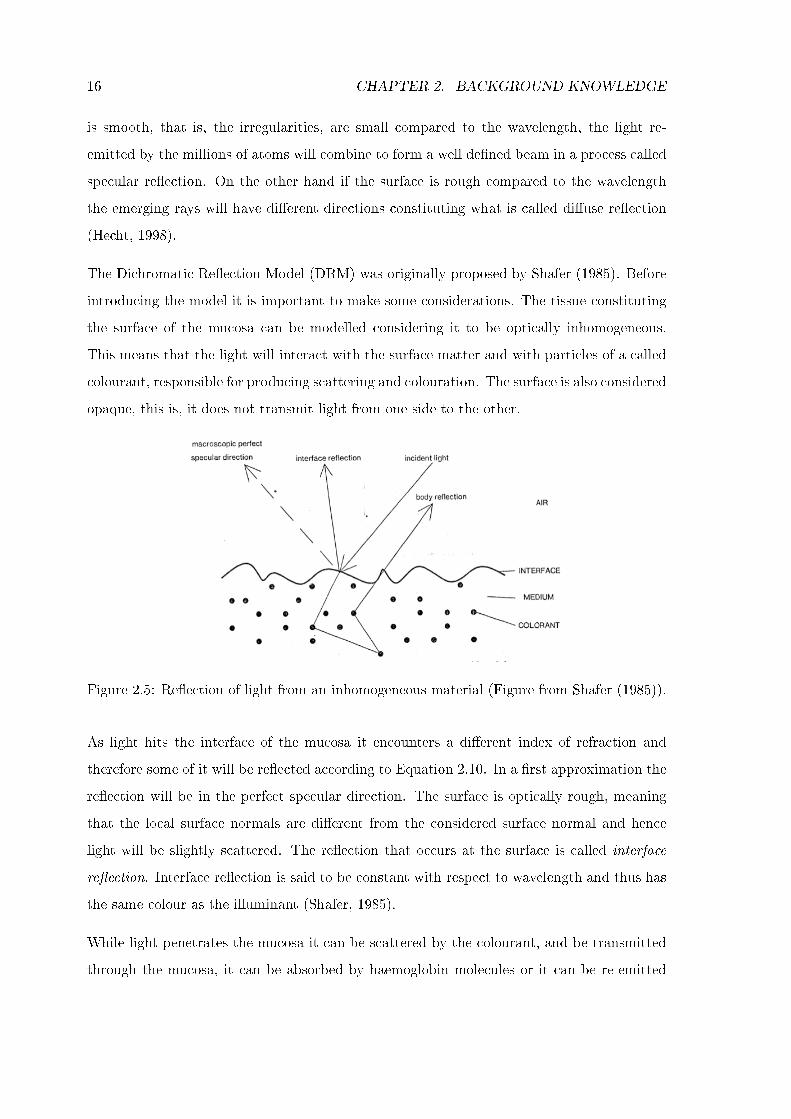
The Dichromatic Re�ection Model (DRM) was originally proposed by Shafer (1985). Before
introducing the model it is important to make some considerations. The tissue constituting
the surface of the mucosa can be modelled considering it to be optically inhomogeneous.
This means that the light will interact with the surface matter and with particles of a called
colourant, responsible for producing scattering and colouration. The surface is also considered
opaque, this is, it does not transmit light from one side to the other.
Figure 2.5: Re�ection of light from an inhomogeneous material (Figure from Shafer (1985)).
As light hits the interface of the mucosa it encounters a di�erent index of refraction and
therefore some of it will be re�ected according to Equation 2.10. In a �rst approximation the
re�ection will be in the perfect specular direction. The surface is optically rough, meaning
that the local surface normals are di�erent from the considered surface normal and hence
light will be slightly scattered. The re�ection that occurs at the surface is called interface
re�ection. Interface re�ection is said to be constant with respect to wavelength and thus has
the same colour as the illuminant (Shafer, 1985).
While light penetrates the mucosa it can be scattered by the colourant, and be transmitted
through the mucosa, it can be absorbed by haemoglobin molecules or it can be re-emitted
2.4. THE DICHROMATIC REFLECTION MODEL 17
through the mucosal surface, producing the body re�ection as illustrated in Figure 2.5. The
geometric distribution of light resulting from the body re�ection is considered isotropic,
meaning independent of the viewing angle. Its colour will be di�erent from the illuminant
because absorption or scattering occurs and their probabilities are wavelength dependent.
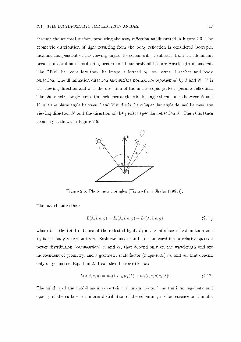
The DRM then considers that the image is formed by two terms: interface and body
re�ection. The illumination direction and surface normal are represented by I and N . V is
the viewing direction and J is the direction of the macroscopic perfect specular re�ection.
The photometric angles are i, the incidence angle, e is the angle of emittance between N and
V , g is the phase angle between I and V and s is the o�-specular angle de�ned between the
viewing direction N and the direction of the perfect specular re�ection J . The re�ectance
geometry is shown in Figure 2.6.
Figure 2.6: Photometric Angles (Figure from Shafer (1985)).
The model states that:
L(λ, i, e, g) = Li(λ, i, e, g) + Lb(λ, i, e, g) (2.11)
where L is the total radiance of the re�ected light, Li is the interface re�ection term and
Lb is the body re�ection term. Both radiances can be decomposed into a relative spectral
power distribution (composition) ci and cb, that depend only on the wavelength and are
independent of geometry, and a geometric scale factor (magnitude) mi and mb that depend
only on geometry. Equation 2.11 can then be rewritten as:
L(λ, i, e, g) = mi(i, e, g)ci(λ) +mb(i, e, g)cb(λ); (2.12)
The validity of the model assumes certain circumstances such as the inhomogeneity and
opacity of the surface, a uniform distribution of the colourant, no �uorescence or thin-�lm
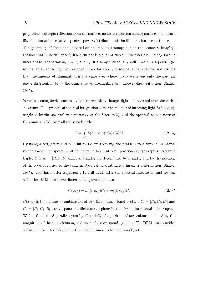
18 CHAPTER 2. BACKGROUND KNOWLEDGE
properties, isotropic re�ection from the surface, no inter-re�ection among surfaces, no di�use
illumination and a relative spectral power distribution of the illumination across the scene.
The generality of the model is based on not making assumptions on the geometry imaging,
the fact that it doesn't specify if the surface is planar or curve, it does not assume any speci�c
functions for the terms mi, mb, ci and cb. It also applies equally well if we have a point light
source, an extended light source or in�nitely far way light source. Finally it does not assume
that the amount of illumination is the same everywhere in the scene but only the spectral
power distribution to be the same thus approximating to a more realistic situation (Shafer,
1985).
When a sensing device such as a camera records an image, light is integrated over the entire
spectrum. This process of spectral integration sums the amount of incoming light L(λ, i, e, g),
weighted by the spectral transmittance of the �lter, τ(λ), and the spectral responsivity of
the camera, s(λ), over all the wavelengths:
C =
∫
λL(λ, i, e, g)τ(λ)s(λ)dλ (2.13)
By using a red, green and blue �lters we are reducing the problem to a three dimensional
vector space. The spectrum of an incoming beam at pixel position (x, y) is represented by a
triplet C(x, y) = [R,G,B] where i, e and g are determined by x and y and by the position
of the object relative to the camera. Spectral integration is a linear transformation (Shafer,
1985). For this matter Equation 2.12 still holds after the spectral integration and we can
write the DRM in a three dimensional space as follows:
C(x, y) = mi(i, e, g)Ci +mb(i, e, g)Cb (2.14)
C(x, y) is thus a linear combination of two three dimensional vectors, Ci = [Ri, Gi, Bi] and
Cb = [Rb, Gb, Bb], that spans the dichromatic plane in the three dimensional colour space.
Within the de�ned parallelogram by Ci and Cb, the position of any colour is de�ned by the
magnitude of the coe�cients mi and mb at the corresponding point. The DRM thus provides
a mathematical tool to predict the distribution of colours in an object.
Chapter 3
Invariant Features
In this chapter we begin to review some of the literature related to techniques to extract
features from the images. These techniques can be grouped according to their domain:
spatial or frequency, or according to the level they are extracted: high or low level features.
For this task we propose the usage of a local descriptor based on spatial domain features.
These features are proved to be invariant to scale, rotation and translation transformations
(Lowe, 2004).
3.1 Related Work
In this section we review some of the work done in the extraction of features and the di�erent
methods that several authors have used in their works to treat and classify all the information
contained in an image, de�nitely worth more then a thousand words.
Spatial Domain Features: In Sousa et al. (2009) adapted colour features combined
with local binary patterns were used in order to build a texture descriptor to natural
endoscopic images. This work was based on Dinis-Ribeiro visual classi�cation for gastric
mucosa and used statistical pattern recognition methodologies to mimic this visual work done
by clinicians. An MPEG-7 visual descriptor for feature extraction in capsule endoscopy was
analysed by Coimbra & Cunha (2006). MPEG-7 is a multimedia content description standard
19
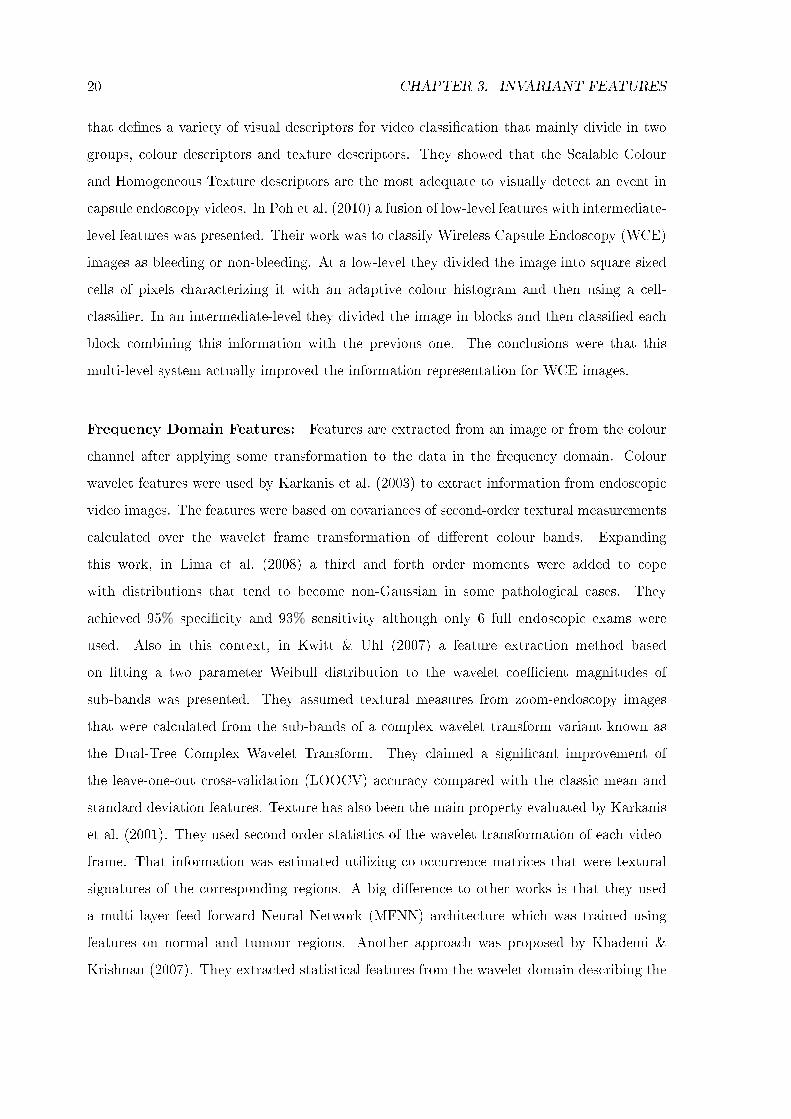
20 CHAPTER 3. INVARIANT FEATURES
that de�nes a variety of visual descriptors for video classi�cation that mainly divide in two
groups, colour descriptors and texture descriptors. They showed that the Scalable Colour
and Homogeneous Texture descriptors are the most adequate to visually detect an event in
capsule endoscopy videos. In Poh et al. (2010) a fusion of low-level features with intermediate-
level features was presented. Their work was to classify Wireless Capsule Endoscopy (WCE)
images as bleeding or non-bleeding. At a low-level they divided the image into square sized
cells of pixels characterizing it with an adaptive colour histogram and then using a cell-
classi�er. In an intermediate-level they divided the image in blocks and then classi�ed each
block combining this information with the previous one. The conclusions were that this
multi-level system actually improved the information representation for WCE images.
Frequency Domain Features: Features are extracted from an image or from the colour
channel after applying some transformation to the data in the frequency domain. Colour
wavelet features were used by Karkanis et al. (2003) to extract information from endoscopic
video images. The features were based on covariances of second-order textural measurements
calculated over the wavelet frame transformation of di�erent colour bands. Expanding
this work, in Lima et al. (2008) a third and forth order moments were added to cope
with distributions that tend to become non-Gaussian in some pathological cases. They
achieved 95% speci�city and 93% sensitivity although only 6 full endoscopic exams were
used. Also in this context, in Kwitt & Uhl (2007) a feature extraction method based
on �tting a two parameter Weibull distribution to the wavelet coe�cient magnitudes of
sub-bands was presented. They assumed textural measures from zoom-endoscopy images
that were calculated from the sub-bands of a complex wavelet transform variant known as
the Dual-Tree Complex Wavelet Transform. They claimed a signi�cant improvement of
the leave-one-out cross-validation (LOOCV) accuracy compared with the classic mean and
standard deviation features. Texture has also been the main property evaluated by Karkanis
et al. (2001). They used second order statistics of the wavelet transformation of each video-
frame. That information was estimated utilizing co-occurrence matrices that were textural
signatures of the corresponding regions. A big di�erence to other works is that they used
a multi layer feed forward Neural Network (MFNN) architecture which was trained using
features on normal and tumour regions. Another approach was proposed by Khademi &
Krishnan (2007). They extracted statistical features from the wavelet domain describing the
3.2. SCALE INVARIANT FEATURE TRANSFORM 21
homogeneity of areas in small bowel images. They explored a shift-invariant discrete wavelet
transform (SWIDWT) claiming a high classi�cation rate.
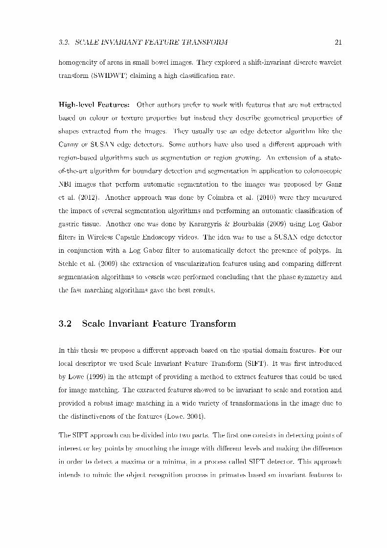
High-level Features: Other authors prefer to work with features that are not extracted
based on colour or texture properties but instead they describe geometrical properties of
shapes extracted from the images. They usually use an edge detector algorithm like the
Canny or SUSAN edge detectors. Some authors have also used a di�erent approach with
region-based algorithms such as segmentation or region growing. An extension of a state-
of-the-art algorithm for boundary detection and segmentation in application to colonoscopic
NBI images that perform automatic segmentation to the images was proposed by Ganz
et al. (2012). Another approach was done by Coimbra et al. (2010) were they measured
the impact of several segmentation algorithms and performing an automatic classi�cation of
gastric tissue. Another one was done by Karargyris & Bourbakis (2009) using Log Gabor
�lters in Wireless Capsule Endoscopy videos. The idea was to use a SUSAN edge detector
in conjunction with a Log Gabor �lter to automatically detect the presence of polyps. In
Stehle et al. (2009) the extraction of vascularization features using and comparing di�erent
segmentation algorithms to vessels were performed concluding that the phase symmetry and
the fast marching algorithms gave the best results.
3.2 Scale Invariant Feature Transform
In this thesis we propose a di�erent approach based on the spatial domain features. For our
local descriptor we used Scale Invariant Feature Transform (SIFT). It was �rst introduced
by Lowe (1999) in the attempt of providing a method to extract features that could be used
for image matching. The extracted features showed to be invariant to scale and rotation and
provided a robust image matching in a wide variety of transformations in the image due to
the distinctiveness of the features (Lowe, 2004).
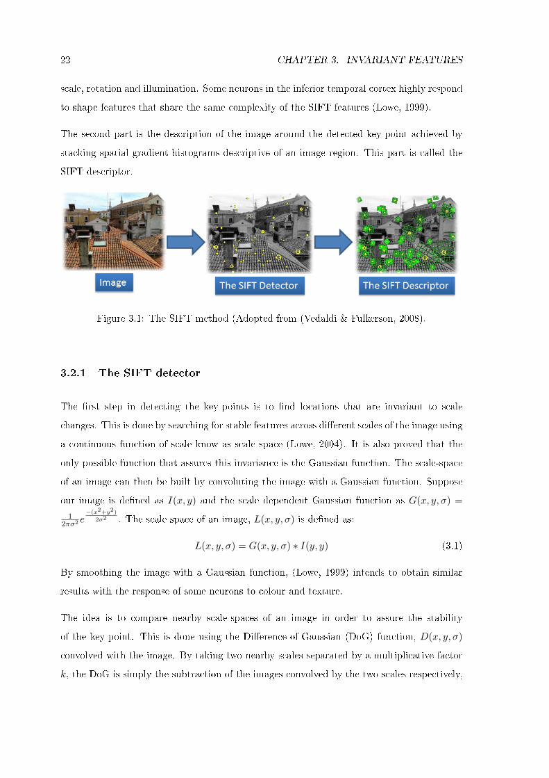
The SIFT approach can be divided into two parts. The �rst one consists in detecting points of
interest or key-points by smoothing the image with di�erent levels and making the di�erence
in order to detect a maxima or a minima, in a process called SIFT detector. This approach
intends to mimic the object recognition process in primates based on invariant features to
22 CHAPTER 3. INVARIANT FEATURES
scale, rotation and illumination. Some neurons in the inferior temporal cortex highly respond
to shape features that share the same complexity of the SIFT features (Lowe, 1999).
The second part is the description of the image around the detected key-point achieved by
stacking spatial gradient histograms descriptive of an image region. This part is called the
SIFT descriptor.
Figure 3.1: The SIFT method (Adopted from (Vedaldi & Fulkerson, 2008).
3.2.1 The SIFT detector
The �rst step in detecting the key-points is to �nd locations that are invariant to scale
changes. This is done by searching for stable features across di�erent scales of the image using
a continuous function of scale know as scale space (Lowe, 2004). It is also proved that the
only possible function that assures this invariance is the Gaussian function. The scale-space
of an image can then be built by convoluting the image with a Gaussian function. Suppose
our image is de�ned as I(x, y) and the scale dependent Gaussian function as G(x, y, σ) =
12πσ2 e
−(x2+y2)
2σ2 . The scale space of an image, L(x, y, σ) is de�ned as:
L(x, y, σ) = G(x, y, σ) ∗ I(y, y) (3.1)
By smoothing the image with a Gaussian function, (Lowe, 1999) intends to obtain similar
results with the response of some neurons to colour and texture.
The idea is to compare nearby scale-spaces of an image in order to assure the stability
of the key-point. This is done using the Di�erence-of-Gaussian (DoG) function, D(x, y, σ)
convolved with the image. By taking two nearby scales separated by a multiplicative factor
k, the DoG is simply the subtraction of the images convolved by the two scales respectively,
3.2. SCALE INVARIANT FEATURE TRANSFORM 23
and is given by:
D(x, y, σ) = L(x, y, kσ)− L(x, y, σ) (3.2)
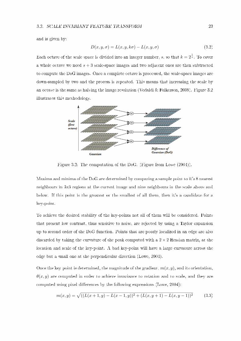
Each octave of the scale space is divided into an integer number, s, so that k = 21s . To cover
a whole octave we need s+ 3 scale-space images and two adjacent ones are then subtracted
to compute the DoG images. Once a complete octave is processed, the scale-space images are
down-sampled by two and the process is repeated. This means that increasing the scale by
an octave is the same as halving the image resolution (Vedaldi & Fulkerson, 2008). Figure 3.2
illustrates this methodology.
Figure 3.2: The computation of the DoG. (Figure from Lowe (2004)).
Maxima and minima of the DoG are determined by comparing a sample point to it's 8 nearest
neighbours in 3x3 regions at the current image and nine neighbours in the scale above and
below. If this point is the greatest or the smallest of all them, then it's a candidate for a
key-point.
To achieve the desired stability of the key-points not all of them will be considered. Points
that present low contrast, thus sensitive to noise, are rejected by using a Taylor expansion
up to second order of the DoG function. Points that are poorly localized in an edge are also
discarded by taking the curvature of the peak computed with a 2× 2 Hessian matrix, at the
location and scale of the key-point. A bad key-point will have a large curvature across the
edge but a small one at the perpendicular direction (Lowe, 2004).
Once the key-point is determined, the magnitude of the gradient, m(x, y), and its orientation,
θ(x, y) are computed in order to achieve invariance to rotation and to scale, and they are
computed using pixel di�erences by the following expressions (Lowe, 2004):
m(x, y) =√
((L(x+ 1, y)− L(x− 1, y))2 + (L(x, y + 1)− L(x, y − 1))2 (3.3)
24 CHAPTER 3. INVARIANT FEATURES
θ(x, y) = tan−1[L(x, y + 1)− L(x, y − 1)
L(x+ 1, y)− L(x− 1, y)
](3.4)
The SIFT detector is a circle of radius equal to the scale. A geometric frame of four
parameters will describe the key-point. The x and y position of the center of the key-point
determined by Equation 3.3, it's scale, s and orientation θ given by Equation 3.4.
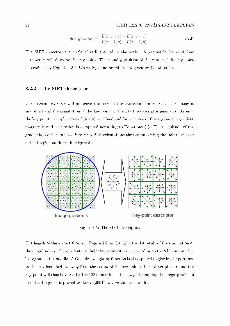
3.2.2 The SIFT descriptor
The determined scale will in�uence the level of the Gaussian blur at which the image is
smoothed and the orientation of the key-point will rotate the descriptor geometry. Around
the key-point a sample array of 16×16 is de�ned and for each one of this regions the gradient
magnitude and orientation is computed according to Equations 3.3. The magnitude of the
gradients are then stacked into 8 possible orientations thus summarizing the information of
a 4× 4 region as shown in Figure 3.3.
Figure 3.3: The SIFT descriptor.
The length of the arrows shown in Figure 3.2 on the right are the result of the summation of
the magnitudes of the gradients to their closest orientations according to the 8 bin orientation
histogram in the middle. A Gaussian weighting function is also applied to give less importance
to the gradients farther away from the center of the key-points. Each descriptor around the
key-point will thus have 8×4×4 = 128 dimensions. This way of sampling the image gradients
into 4× 4 regions is proved by Lowe (2004) to give the best results.
3.2. SCALE INVARIANT FEATURE TRANSFORM 25
3.2.3 Sampling Strategies
The SIFT approach consists in calculating the position of a key-point by computing the DoG
and extract the desired features around that key-point. The features consist of the computed
gradients stacked in a spatial histogram that contains information of a 4x4 region. But a
question arises. What is the best sampling strategy to use in this set of images? Should we
determine the location of the key-point or could we skip that part of the SIFT approach and
perform a di�erent type of sampling? According to Nowak et al. (2006) the performance of
a classi�er based on SIFT features increases with an increasing number of points per image.
They also concluded that for a high number of points the best way of sampling an image was
to perform a uniform random sampling (Nowak et al., 2006). With this in mind and knowing
we have images whose textures are spread over a region, thus having a considerable number
of points per image, we chose to perform a dense sampling of the SIFT descriptors. This way
of densely sampling an image is called a DSIFT. It consists in skipping the detection stage
of the key-points. The idea is to place a quadrangular grid of key-points on top of the image
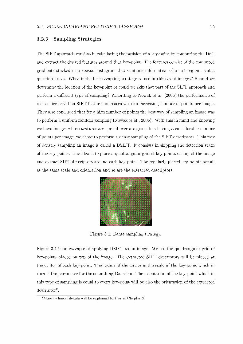
and extract SIFT descriptors around each key-point. The regularly placed key-points are all
at the same scale and orientation and so are the extracted descriptors.
Figure 3.4: Dense sampling strategy.
Figure 3.4 is an example of applying DSIFT to an image. We see the quadrangular grid of
key-points placed on top of the image. The extracted SIFT descriptors will be placed at
the center of each key-point. The radius of the circles is the scale of the key-point which in
turn is the parameter for the smoothing Gaussian. The orientation of the key-point which in
this type of sampling is equal to every key-point will be also the orientation of the extracted
descriptor2.
2More technical details will be explained further in Chapter 6.

26 CHAPTER 3. INVARIANT FEATURES
Chapter 4
Adding Colour Information
With the Dichromatic Re�ection Model, presented in Section 2.4, in this Chapter we seek
alternative formulations for the RGB colours in an attempt to improve the results obtained
by a regular conversion to gray-scale. The RGB colour system and some of its proper-
ties are brie�y presented as well as the opponent process theory and the derivation of
the mathematical expressions of the opponent colours. These colour systems are endowed
by important photometric invariance properties that augment the robustness of posterior
recognition process.
4.1 Colour Spaces
We saw in Section 2.4 that the spectrum of an incoming beam at position (x, y) is given by
Equation 2.13. Most of the device manufacturers opted to use a red, green and blue �lter
and the sensitivities of each �lter are reasonably well matched to the human eye. By doing
so, we are reducing the problem to three dimensions and thus the spectrum of the incoming
beam is represented by a triplet C = [R,G,B].
RGB Colour System: The RGB colour system is an additive colour model. A broad array
of colours can be reproduced by adding certain amounts of red, green and blue. We can then
build a colour cube de�ned by the R, G and B axis. White is produced when all colours are
27
28 CHAPTER 4. ADDING COLOUR INFORMATION
at a maximum light intensity. Black on the other hand is produced when all colours are at
a minimum light intensity, the origin of the referential. The diagonal connecting the white
and black corners of the RGB cube de�nes the intensity:
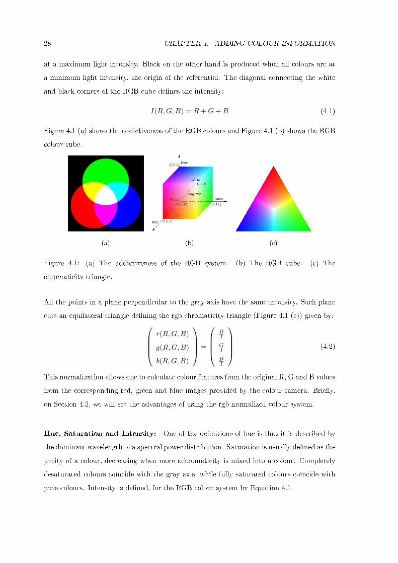
I(R,G,B) = R+G+B (4.1)
Figure 4.1 (a) shows the addictiveness of the RGB colours and Figure 4.1 (b) shows the RGB
colour cube.
(a) (b) (c)
Figure 4.1: (a) The addictiveness of the RGB system. (b) The RGB cube. (c) The
chromaticity triangle.
All the points in a plane perpendicular to the gray axis have the same intensity. Such plane
cuts an equilateral triangle de�ning the rgb chromaticity triangle (Figure 4.1 (c)) given by:
r(R,G,B)
g(R,G,B)
b(R,G,B)
=
RI
GI
BI
(4.2)
This normalization allows one to calculate colour features from the original R, G and B values
from the corresponding red, green and blue images provided by the colour camera. Brie�y,
on Section 4.2, we will see the advantages of using the rgb normalized colour system.
Hue, Saturation and Intensity: One of the de�nitions of hue is that it is described by
the dominant wavelength of a spectral power distribution. Saturation is usually de�ned as the
purity of a colour, decreasing when more achromaticity is mixed into a colour. Completely
desaturated colours coincide with the gray axis, while fully saturated colours coincide with
pure colours. Intensity is de�ned, for the RGB colour system by Equation 4.1.
4.1. COLOUR SPACES 29
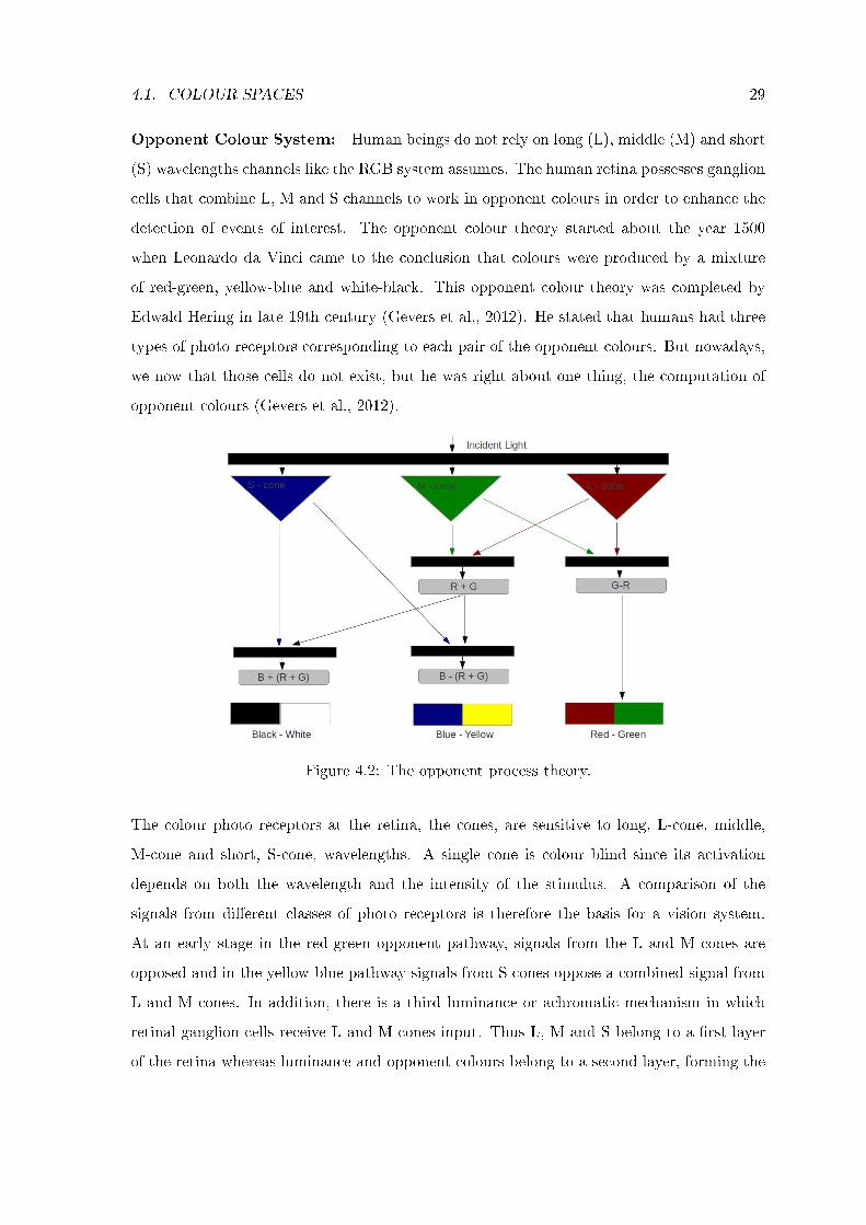
Opponent Colour System: Human beings do not rely on long (L), middle (M) and short
(S) wavelengths channels like the RGB system assumes. The human retina possesses ganglion
cells that combine L, M and S channels to work in opponent colours in order to enhance the
detection of events of interest. The opponent colour theory started about the year 1500
when Leonardo da Vinci came to the conclusion that colours were produced by a mixture
of red-green, yellow-blue and white-black. This opponent colour theory was completed by
Edwald Hering in late 19th century (Gevers et al., 2012). He stated that humans had three
types of photo receptors corresponding to each pair of the opponent colours. But nowadays,
we now that those cells do not exist, but he was right about one thing, the computation of
opponent colours (Gevers et al., 2012).
Figure 4.2: The opponent process theory.
The colour photo receptors at the retina, the cones, are sensitive to long, L-cone, middle,
M-cone and short, S-cone, wavelengths. A single cone is colour blind since its activation
depends on both the wavelength and the intensity of the stimulus. A comparison of the
signals from di�erent classes of photo receptors is therefore the basis for a vision system.
At an early stage in the red-green opponent pathway, signals from the L and M cones are
opposed and in the yellow-blue pathway signals from S cones oppose a combined signal from
L and M cones. In addition, there is a third luminance or achromatic mechanism in which
retinal ganglion cells receive L and M cones input. Thus L, M and S belong to a �rst layer
of the retina whereas luminance and opponent colours belong to a second layer, forming the
30 CHAPTER 4. ADDING COLOUR INFORMATION
basis of chromatic input to the visual primary cortex.
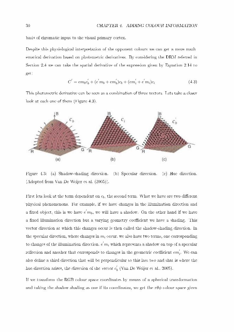
Despite this physiological interpretation of the opponent colours we can get a more math-
ematical derivation based on photometric derivatives. By considering the DRM referred in
Section 2.4 we can take the spatial derivative of the expression given by Equation 2.14 to
get:
C′
= embc′b + (e
′mb + em
′b)cb + (em
′i + e
′mi)ci (4.3)
This photometric derivative can be seen as a combination of three vectors. Lets take a closer
look at each one of them (Figure 4.3).
Figure 4.3: (a) Shadow-shading direction. (b) Specular direction. (c) Hue direction.
(Adopted from Van De Weijer et al. (2005)).
First lets look at the term dependent on cb, the second term. What we have are two di�erent
physical phenomenons. For example, if we have changes in the illumination direction and
a �xed object, this is we have e′mb, we will have a shadow. On the other hand if we have
a �xed illumination direction but a varying geometry coe�cient we have a shading. This
vector direction at which this changes occur is then called the shadow-shading direction. In
the specular direction, where changes in mi occur, we also have two terms, one corresponding
to changes of the illumination direction, e′mi which represents a shadow on top of a specular
re�ection and another that corresponds to changes in the geometric coe�cient em′i. We can
also de�ne a third direction that will be perpendicular to this last two and that is where the
hue direction arises, the direction of the vector c′b (Van De Weijer et al., 2005).
If we transform the RGB colour space coordinates by means of a spherical transformation
and taking the shadow-shading as one if its coordinates, we get the rθφ colour space given
4.2. PHOTOMETRIC INVARIANT FEATURES 31
by:
r
θ
φ
=
√R2 +G2 +B2 = |C|
arctan GR
arcsin√R2+G2√
R2+G2+B2
(4.4)
On the other hand if we take the specular direction as a component of a new orthogonal
space we get the opponent colour space, which for a known illuminant cs = (α, β, γ)T , is
given by:
O1
O2
O3
=
βR−αG√α2+β2
αγR+βγG−(α2+β2)B√(α2+β2+γ2)(α2+β2)
αR+βG+γB√α2+β2+γ2
(4.5)
By taking white illumination the source term is cs = (1, 1, 1)T , and so the opponent colour
formulas simplify into:
O1
O2
O3
=
R−G√2
R+G−2B√6
R+G+B√3
(4.6)
If we take the hue direction as a component for a new coordinate system we get the hue-
saturation-intensity for the opponent colours, simply by considering a polar coordinate
transformation of the Red Green Blue (RGB) colour space and are given by:
h
s
i
=
arctan(O1O2
)
√O2
1 +O22
O3
=
arctan(√
3(R−G)R+G−2B
)√
46(R2 +G2 +B2 −RG−RB −GB)
R+G+B3√3
(4.7)
O1 roughly corresponds to the red-green channel, O2 to the yellow-blue channel and O3 to the
intensity channel. The opponent colour system largely decorrelates the RGB colour channels
although it is device dependent and it is not perceptually uniform, this is, the numerical
distance between to colours cannot be related to perceptual di�erences.
4.2 Photometric Invariant Features
The DRM can be applied to derive photometrically invariant features. If we assume only
matte, or dull surfaces, specular re�ection is negligible, this is mi = 0. The angles i, e and
32 CHAPTER 4. ADDING COLOUR INFORMATION
g fully specify the location of the pixel so we can simplify the notation by denoting ρ as the
spatial coordinates, and so Equation 2.14 reduces to the Lambertian model for di�use body
re�ection:
C(ρ) = mb(ρ)Cb (4.8)
A zero-order invariant can be obtained building each channel with the assumption given in
Equation 4.8. This way the normalized rgb can be considered invariant to lighting geometry
and viewpoint, this is, independent of mb, since:
r =R
R+G+B=
mb(ρ)CRbmb(ρ)(CRb + CGb + CBb
=CRb
CRb + CGb + CBb(4.9)
Similar equations can be obtained for the normalized g and b. It thus results in the indepen-
dence for the surface orientation, illumination direction and illumination intensity, assuming
Lambertian re�ection and white illumination. This normalized rgb space depends only on
the factors CRb , CGb and CBb which depend on the sensor and the surface albedo (Gevers
et al., 2012).
gray r g
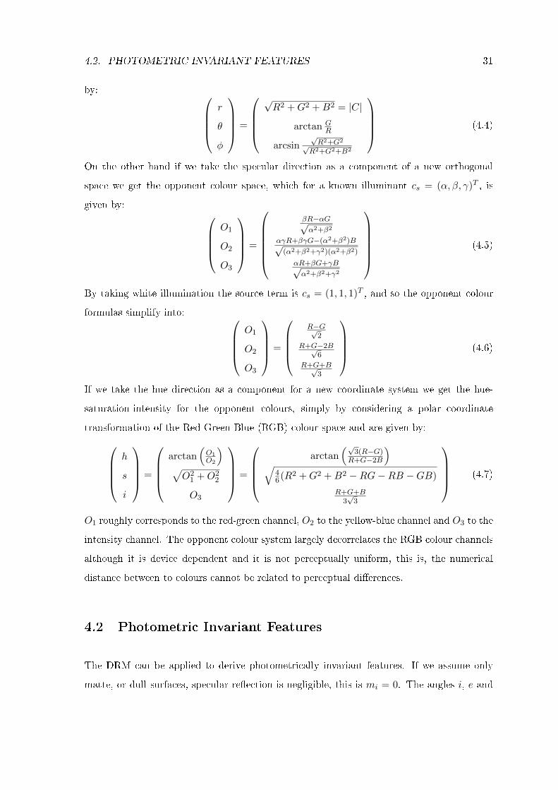
Figure 4.4: Gray-scale image and the r and g channels.
In fact with the DRM applied to each channel we can perform any linear combination. One
of the reasons to do so is the possibility to capture intensity variations in regular surfaces.
This way we have to analyse the proportion of these variations in order to diminish this
dependency. That said we can compute:
CRGB =
∑i ai(C
R)pi (CG)qi (C
B)ri∑j bj(C
R)sj(CG)tj(C
B)uj
=
∑i ai(mb(ρ)CRb )pi (mb(ρ)CGb )qi (mb(ρ)CBb )ri∑
j bj(mb(rho)CRb )sj(mb(ρ)CGb )tj(mb(ρ)CBb )uj
=
∑i aimb(ρ)p+q+r(CR)pi (C
G)qi (CB)ri∑
j bjmb(ρ)s+t+u(CR)sj(CG)tj(C
B)uj
(4.10)
4.2. PHOTOMETRIC INVARIANT FEATURES 33
Since p+ q + r = s+ t+ u, Equation 4.10 can be further simpli�ed to:
CRGB =
∑i ai(C
Rb )pi (C
Gb )qi (C
Bb )ri∑
i bi(CRb )sj(C
Gb )tj(C
Bb )uj
(4.11)
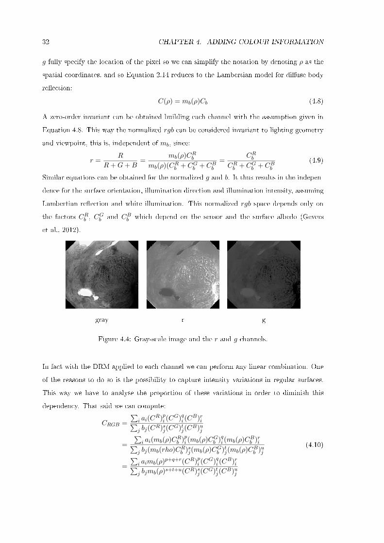
Numerous invariants can be obtained. The set of �rst-order invariants involves the set where
p+ q + r = s+ t+ u = 1: {R
G,R
B,G
B, · · ·
}(4.12)
This set of invariants show the same invariance properties as the normalized rgb colours.
RG
RB
GB
Figure 4.5: The ratio of the channels.
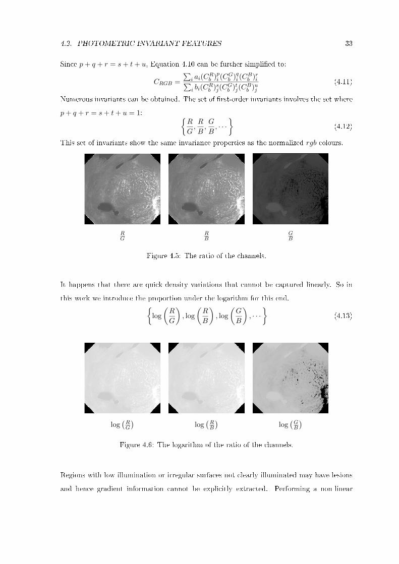
It happens that there are quick density variations that cannot be captured linearly. So in
this work we introduce the proportion under the logarithm for this end.{
log
(R
G
), log
(R
B
), log
(G
B
), · · ·
}(4.13)
log(RG
)log(RB
)log(GB
)
Figure 4.6: The logarithm of the ratio of the channels.
Regions with low illumination or irregular surfaces not clearly illuminated may have lesions
and hence gradient information cannot be explicitly extracted. Performing a non-linear
34 CHAPTER 4. ADDING COLOUR INFORMATION
mapping on the combined colour system will provide the necessary enhancement to properly
analyse the variations of these proportions. For instance, darker regions will have high slopes
of information variations whereas lighter regions will have slower variations (e.g., specular
highlights).
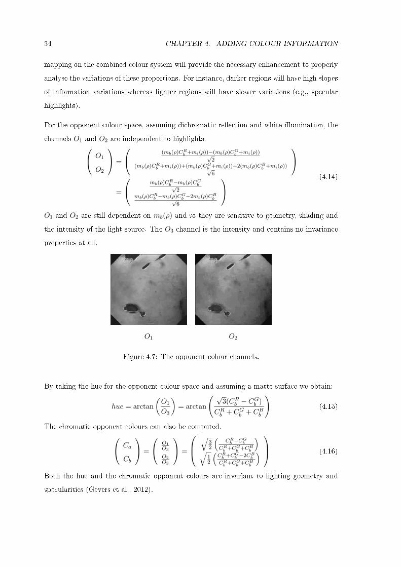
For the opponent colour space, assuming dichromatic re�ection and white illumination, the
channels O1 and O2 are independent to highlights. O1
O2
=
(mb(ρ)CRb +mi(ρ))−(mb(ρ)CGb +mi(ρ))√
2(mb(ρ)C
Rb +mi(ρ))+(mb(ρ)C
Gb +mi(ρ))−2(mb(ρ)CBb +mi(ρ))√6
=
mb(ρ)CRb −mb(ρ)C
Gb√
2mb(ρ)C
Rb −mb(ρ)C
Gb −2mb(ρ)C
Bb√
6
(4.14)
O1 and O2 are still dependent on mb(ρ) and so they are sensitive to geometry, shading and
the intensity of the light source. The O3 channel is the intensity and contains no invariance
properties at all.
O1 O2
Figure 4.7: The opponent colour channels.
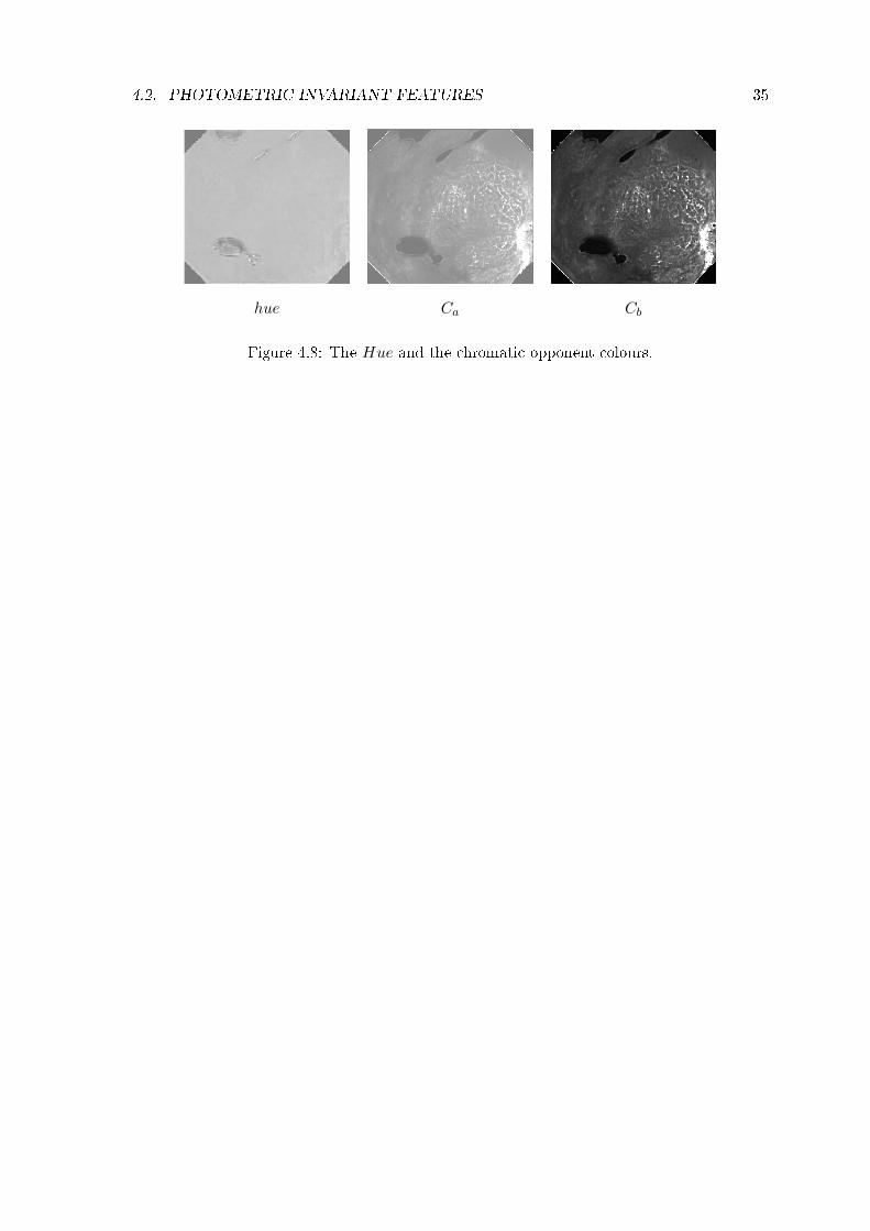
By taking the hue for the opponent colour space and assuming a matte surface we obtain:
hue = arctan
(O1
O3
)= arctan
( √3(CRb − CGb )
CRb + CGb + CBb
)(4.15)
The chromatic opponent colours can also be computed.
Ca
Cb
=
O1O3
O2O3
=
√32
(CRb −C
Gb
CRb +CGb +CBb
)
√12
(CRb +CGb −2C
Bb
CRb +CGb +CBb
)
(4.16)
Both the hue and the chromatic opponent colours are invariant to lighting geometry and
specularities (Gevers et al., 2012).
4.2. PHOTOMETRIC INVARIANT FEATURES 35
hue Ca Cb
Figure 4.8: The Hue and the chromatic opponent colours.

36 CHAPTER 4. ADDING COLOUR INFORMATION
Chapter 5
Pathology Recognition
We saw in Chapter 3 how to extract features from the images and based on the DRM we
obtained special photometric invariant features in Chapter 4. In Section 2.2 the images were
grouped into two classes according to Singh's taxonomy. But know a question arises. How
can we actually build a CAD system to help us automatically classify these images? For this
matter we will resort to a powerful classi�cation tool known as Support Vector Machine, a
learning mechanism that became very popular two decades ago. For self-contained reasons
of this document we will review the concepts behind SVMs.
5.1 Linearly Separable Binary Classi�cation
The design of automatic learning algorithms is one classic research problem from the pattern
recognition community. The most well-known problem is classi�cation. The idea is to take
some input vector x and assign it to some discrete class, Ck where k = 1, ...K. The input
feature space will be divided into decision regions, bounded by a called decision boundary. If
the data set has classes that can be separated exactly by a computed linear decision boundary,
the classes are said to be linearly separable. The simplest way of doing this is to construct a
linear discriminant function that takes an input vector x and directly assigns it to a speci�c
class. It is represented by the following expression:
g(x) = wTx+ w0 (5.1)
37
38 CHAPTER 5. PATHOLOGY RECOGNITION
where w is the weight vector and w0 is a bias parameter (Bishop & Nasrabadi, 2006).
Reducing the problem to two classes, say C1 and C2 and assuming we have an input vector x,
the linear discriminant function will assign it to class C1 if g(x) > 0 and to class C2 otherwise.
The decision boundary is de�ned as g(x) = 0. If the feature space is D-dimensional, the
decision boundary will be (D+1)-dimensional.
For any two points, xa and xb lying on the decision surface, we have that wTxa + w0 =
wTxb + w0, in other words wT (xa − xb) = 0, which indicates that w is normal to any vector
lying in the decision boundary and thus de�nes the orientation of the decision surface.
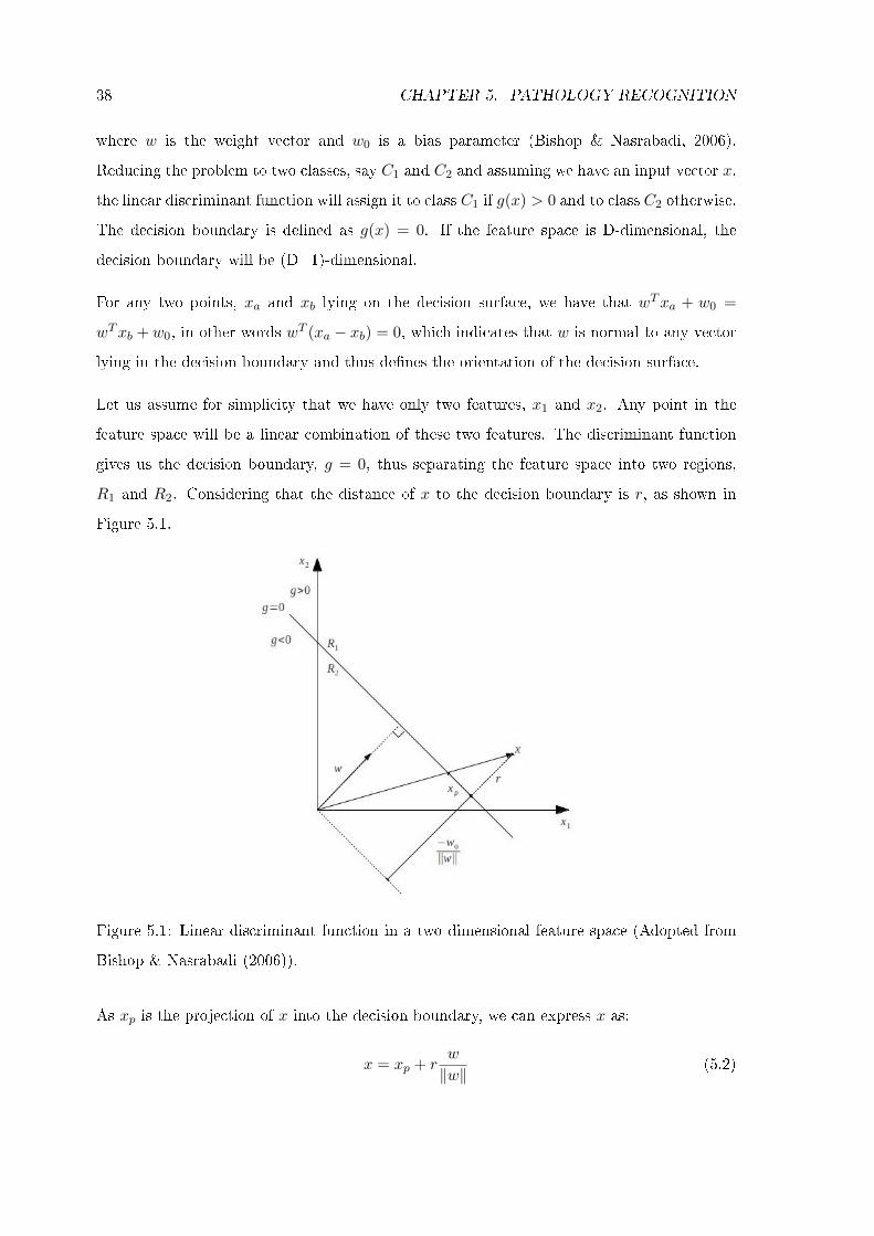
Let us assume for simplicity that we have only two features, x1 and x2. Any point in the
feature space will be a linear combination of these two features. The discriminant function
gives us the decision boundary, g = 0, thus separating the feature space into two regions,
R1 and R2. Considering that the distance of x to the decision boundary is r, as shown in
Figure 5.1.
Figure 5.1: Linear discriminant function in a two dimensional feature space (Adopted from
Bishop & Nasrabadi (2006)).
As xp is the projection of x into the decision boundary, we can express x as:
x = xp + rw
‖w‖ (5.2)
5.1. LINEARLY SEPARABLE BINARY CLASSIFICATION 39
But xp lies on the decision boundary and therefore g(xp) = 0, so multiplying both sides of
the equation by wT and adding w0, we obtain (Bishop & Nasrabadi, 2006):
g(x) = wTx+ w0 = r‖w‖ (5.3)
which gives
r =g(x)
‖w‖ (5.4)
The linear discriminant thus divides the feature space through a decision boundary or
hyperplane if we have more than two dimensions. The orientation of the hyperplane is
controlled by the weight vector w and the bias parameter w0 controls the location of the
hyperplane relative to the origin of the feature space. The linear discriminant function g(x)
gives us a signed measure of the perpendicular distance of x to the decision boundary as
demonstrated by Equation 5.4 (Bishop & Nasrabadi, 2006).
SVM rely on the same principles, but they represent the data in a much higher dimension
than the original feature space by means of a linear mapping, φ(x).
g(x) = wTφ(x) + b (5.5)
where b is the bias parameter. Lets assume, as before, we have N input vectors x1, xn, ..., xN
with the corresponding labels y1, yn, ..., yN where yn ∈ {−1, 1}. The transformed data points
by means of φ(x) will be classi�ed according to the sign of g(x). Lets also assume the case
where the training data set is linearly separable, this is, Equation 5.5 has at least one solution,
satisfying the condition g(xn) ≥ 0 for points with label yn = +1 and g(xn) < 0 for points
with yn = −1. But multiple solutions may arise. We must then �nd the solution with the
smallest generalization error (Bishop & Nasrabadi, 2006).
SVM makes use of the called Support Vectors, the points that are closest to the decision
boundary. This distance is called the margin and the idea behind the SVM is to maximize
this margin.
In Figure 5.2 we have two classes represented by the green and blue dots and the respective
support vectors represented by a yellow contour. x′1 and x
′2 are the transformed features by
means of φ(x). m1 and m2 are the respective distances to the hyperplane separating the two
classes. To implement a SVM we need to calculate the variables w and b so that our training
40 CHAPTER 5. PATHOLOGY RECOGNITION
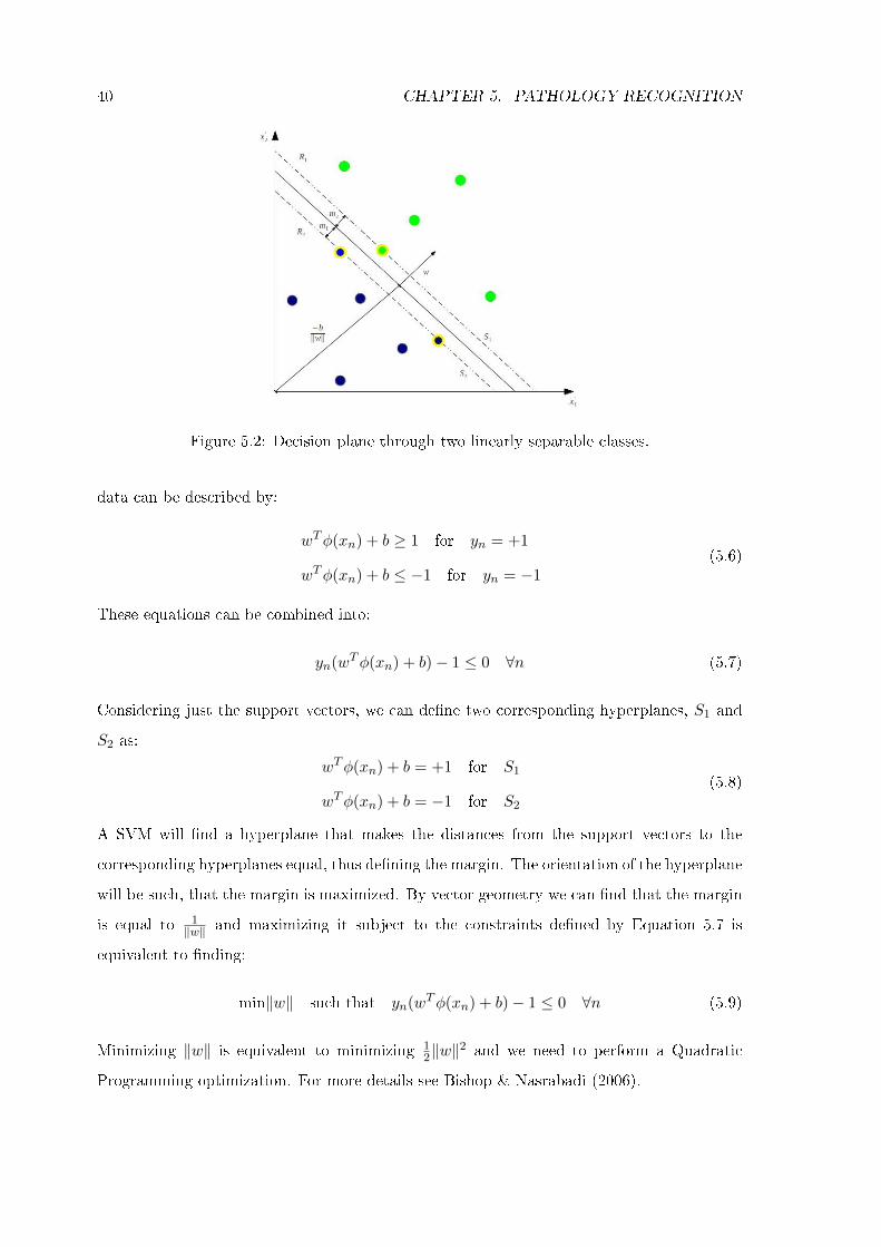
Figure 5.2: Decision plane through two linearly separable classes.
data can be described by:
wTφ(xn) + b ≥ 1 for yn = +1
wTφ(xn) + b ≤ −1 for yn = −1(5.6)
These equations can be combined into:
yn(wTφ(xn) + b)− 1 ≤ 0 ∀n (5.7)
Considering just the support vectors, we can de�ne two corresponding hyperplanes, S1 and
S2 as:
wTφ(xn) + b = +1 for S1
wTφ(xn) + b = −1 for S2
(5.8)
A SVM will �nd a hyperplane that makes the distances from the support vectors to the
corresponding hyperplanes equal, thus de�ning the margin. The orientation of the hyperplane
will be such, that the margin is maximized. By vector geometry we can �nd that the margin
is equal to 1‖w‖ and maximizing it subject to the constraints de�ned by Equation 5.7 is
equivalent to �nding:
min‖w‖ such that yn(wTφ(xn) + b)− 1 ≤ 0 ∀n (5.9)
Minimizing ‖w‖ is equivalent to minimizing 12‖w‖2 and we need to perform a Quadratic
Programming optimization. For more details see Bishop & Nasrabadi (2006).
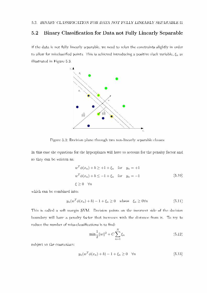
5.2. BINARY CLASSIFICATION FOR DATA NOT FULLY LINEARLY SEPARABLE 41
5.2 Binary Classi�cation for Data not Fully Linearly Separable
If the data is not fully linearly separable, we need to relax the constraints slightly in order
to allow for misclassi�ed points. This is achieved introducing a positive slack variable, ξn as
illustrated in Figure 5.3.
Figure 5.3: Decision plane through two non-linearly separable classes
In this case the equations for the hyperplanes will have to account for the penalty factor and
so they can be written as:
wTφ(xn) + b ≥ +1 + ξn for yn = +1
wTφ(xn) + b ≤ −1 + ξn for yn = −1
ξ ≥ 0 ∀n
(5.10)
which can be combined into:
yn(wTφ(xn) + b)− 1 + ξn ≥ 0 where ξn ≥ 0∀n (5.11)
This is called a soft margin SVM. Decision points on the incorrect side of the decision
boundary will have a penalty factor that increases with the distance from it. To try to
reduce the number of miss-classi�cations is to �nd:
min1
2‖w‖2 + C
N∑
n=1
ξn (5.12)
subject to the constraints:
yn(wTφ(xn) + b)− 1 + ξn ≥ 0 ∀n (5.13)
42 CHAPTER 5. PATHOLOGY RECOGNITION
where the parameter C controls the trade-o� between the slack variable penalty and the size
of the margin. See Bishop & Nasrabadi (2006) for more details.
5.3 Non-linear Support Vector Machine
When applying our SVM to linearly separable data we create a matrix H, from the dot
product of our input variables.
Hn,m = ynymK(xn, xm) = xn · xm = xTnxm (5.14)
K(xn, xm) is an example of a family of functions called Kernel functions, where K(xn, xm)
is the Linear kernel. There are other kernel functions as the Intersection kernel de�ned as
KHI(xn, xm) = min(xn, xm) or the χ2 kernel, Kχ2 = 2xtnxmxn+xm
. These special functions allow
to transform the features into a higher dimensional space, so that the data can actually be
completely separated and we can classify our images based on the constructed decision plane.
We shall not enter in many details as this is a wide subject and is out of the scope of this
thesis1.
1For a more detailed description on this subject see Shawe-Taylor & Cristianini (2004)
Chapter 6
Experimental Study
We begin this chapter by presenting the image dataset used in these experiments and the
separation that we performed in order to build a training set and a test set. We also present
the used methodology to extract features from the images in order to properly recognize
lesions in the tissues. The method consists of extracting SIFT features, sampling the
descriptors with a regular grid. The method to construct new image histograms is also
presented forming the vocabulary of each image. These new histograms will be the input
for our classi�er. As we saw in Chapter 5 the classi�cation step will be performed using
a Support Vector Machine (SVM). The methods that we used in order to optimize the
classi�cation process and to assess the classi�er performance are also presented.
6.1 Image dataset
The image set is composed of endoscopic images from the Barrett's oesophagus, collected by
a research group. We have a total of 250 images classi�ed according to Singh's classi�cation
proposal (Singh et al., 2008) as presented in Section 2.2. They were also annotated, this
is, the region of interest was selected in order to discard irrelevant information, by clinical
experts with di�erent expertises. In this thesis the images were grouped into two classes,
normal (C1) versus pathologic (C2), reducing the problem to a binary classi�cation system.
Type A images are normal, they do not present any kind of irregularity either in the pit
patterns or in the microvasculature. Types B, C and D do show some irregularities and may
43
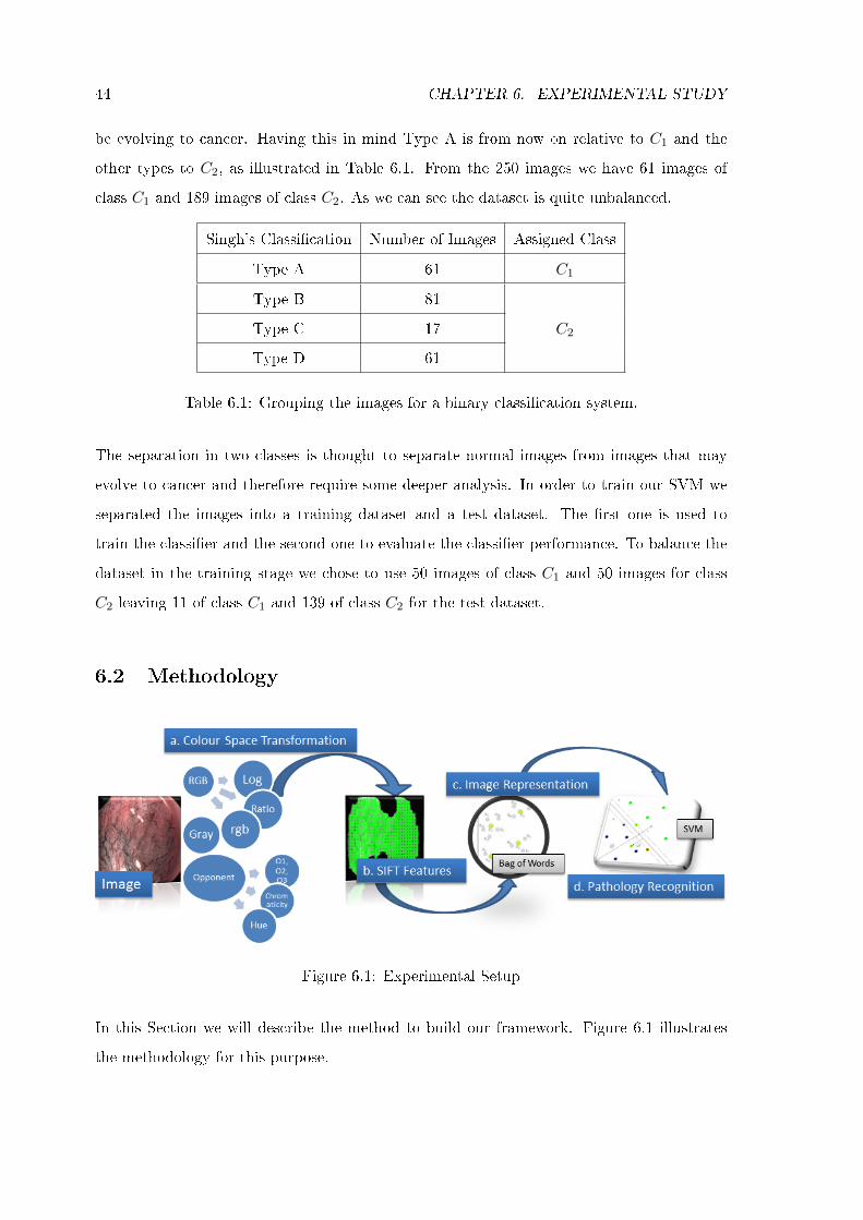
44 CHAPTER 6. EXPERIMENTAL STUDY
be evolving to cancer. Having this in mind Type A is from now on relative to C1 and the
other types to C2, as illustrated in Table 6.1. From the 250 images we have 61 images of
class C1 and 189 images of class C2. As we can see the dataset is quite unbalanced.
Singh's Classi�cation Number of Images Assigned Class
Type A 61 C1
Type B 81
C2Type C 17
Type D 61
Table 6.1: Grouping the images for a binary classi�cation system.
The separation in two classes is thought to separate normal images from images that may
evolve to cancer and therefore require some deeper analysis. In order to train our SVM we
separated the images into a training dataset and a test dataset. The �rst one is used to
train the classi�er and the second one to evaluate the classi�er performance. To balance the
dataset in the training stage we chose to use 50 images of class C1 and 50 images for class
C2 leaving 11 of class C1 and 139 of class C2 for the test dataset.
6.2 Methodology
Figure 6.1: Experimental Setup
In this Section we will describe the method to build our framework. Figure 6.1 illustrates
the methodology for this purpose.
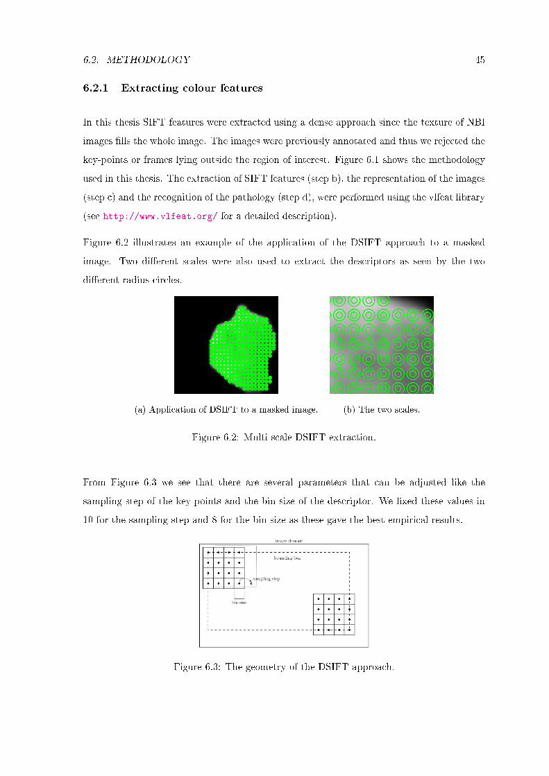
6.2. METHODOLOGY 45
6.2.1 Extracting colour features
In this thesis SIFT features were extracted using a dense approach since the texture of NBI
images �lls the whole image. The images were previously annotated and thus we rejected the
key-points or frames lying outside the region of interest. Figure 6.1 shows the methodology
used in this thesis. The extraction of SIFT features (step b), the representation of the images
(step c) and the recognition of the pathology (step d), were performed using the vlfeat library
(see http://www.vlfeat.org/ for a detailed description).
Figure 6.2 illustrates an example of the application of the DSIFT approach to a masked
image. Two di�erent scales were also used to extract the descriptors as seen by the two
di�erent radius circles.
(a) Application of DSIFT to a masked image. (b) The two scales.
Figure 6.2: Multi-scale DSIFT extraction.
From Figure 6.3 we see that there are several parameters that can be adjusted like the
sampling step of the key-points and the bin size of the descriptor. We �xed these values in
10 for the sampling step and 8 for the bin size as these gave the best empirical results.
Figure 6.3: The geometry of the DSIFT approach.
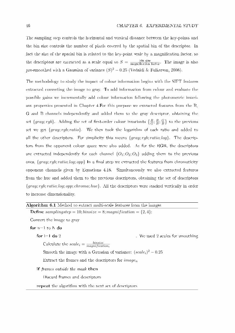
46 CHAPTER 6. EXPERIMENTAL STUDY
The sampling step controls the horizontal and vertical distance between the key-points and
the bin size controls the number of pixels covered by the spatial bin of the descriptor. In
fact the size of the spatial bin is related to the key-point scale by a magni�cation factor, so
the descriptors are extracted at a scale equal to S = bin sizemagni�cation factor
. The image is also
pre-smoothed with a Gaussian of variance (S)2 − 0.25 (Vedaldi & Fulkerson, 2008).
The methodology to study the impact of colour information begins with the SIFT features
extracted converting the image to gray. To add information from colour and evaluate the
possible gains we incrementally add colour information following the photometric invari-
ant properties presented in Chapter 4.For this purpose we extracted features from the R,
G and B channels independently and added them to the gray descriptor, obtaining the
set {gray; rgb}. Adding the set of �rst-order colour invariants{RG ; RB ; GB
}to the previous
set we get {gray; rgb; ratio}. We then took the logarithm of each ratio and added to
all the other descriptors. For simplicity this means {gray; rgb; ratio; log}. The descrip-
tors from the opponent colour space were also added. As for the RGB, the descriptors
are extracted independently for each channel {O1;O2;O3} adding them to the previous
ones, {gray; rgb; ratio; log; opp} In a �nal step we extracted the features from chromaticity
opponent channels given by Equations 4.16. Simultaneously we also extracted features
from the hue and added them to the previous descriptors, obtaining the set of descriptors
{gray; rgb; ratio; log; opp; chroma;hue}. All the descriptors were stacked vertically in order
to increase dimensionality.
Algorithm 6.1 Method to extract multi-scale features from the images
De�ne samplingstep = 10; binsize = 8;magnification = {2, 4};Convert the image to gray
for n=1 to N do
for i=1 do 2 . We used 2 scales for smoothing
Calculate the scalei = binsizemagnificationi
Smooth the image with a Gaussian of variance: (scalei)2 − 0.25
Extract the frames and the descriptors for imagen
if frames outside the mask then
Discard frames and descriptors
repeat the algorithm with the next set of descriptors
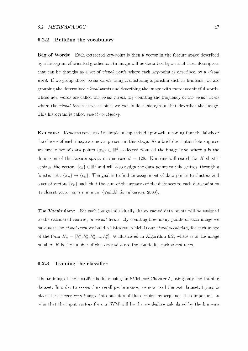
6.2. METHODOLOGY 47
6.2.2 Building the vocabulary
Bag of Words: Each extracted key-point is then a vector in the feature space described
by a histogram of oriented gradients. An image will be described by a set of these descriptors
that can be thought as a set of visual words where each key-point is described by a visual
word. If we group these visual words using a clustering algorithm such as k-means, we are
grouping the determined visual words and describing the image with more meaningful words.
These new words are called the visual terms. By counting the frequency of the visual words
where the visual terms serve as bins, we can build a histogram that describes the image.
This histogram is called visual vocabulary.
K-means: K-means consists of a simple unsupervised approach, meaning that the labels or
the classes of each image are never present in this stage. As a brief description lets suppose
we have a set of data points {xn} ∈ Rd, collected from all the images and where d is the
dimension of the feature space, in this case d = 128. K-means will search for K cluster
centres, the vectors {ck} ∈ Rd and will also assign the data points to this centres, through a
function A : {xn} → {ck}. The goal is to �nd an assignment of data points to clusters and
a set of vectors {ck} such that the sum of the squares of the distances to each data point to
its closest vector ck is minimum (Vedaldi & Fulkerson, 2008).
The Vocabulary: For each image individually the extracted data points will be assigned
to the calculated centres, or visual terms. By counting how many points of each image we
have near the visual term we build a histogram which is our visual vocabulary for each image
of the form Hn = [hn1 , hn2 , h
n3 , ..., h
nk ], as illustrated in Algorithm 6.2, where n is the image
number, K is the number of clusters and h are the counts for each visual term.
6.2.3 Training the classi�er
The training of the classi�er is done using an SVM, see Chapter 5, using only the training
dataset. In order to assess the overall performance, we now used the test dataset, trying to
place these never seen images into one side of the decision hyperplane. It is important to
refer that the input vectors for our SVM will be the vocabulary calculated by the k-means
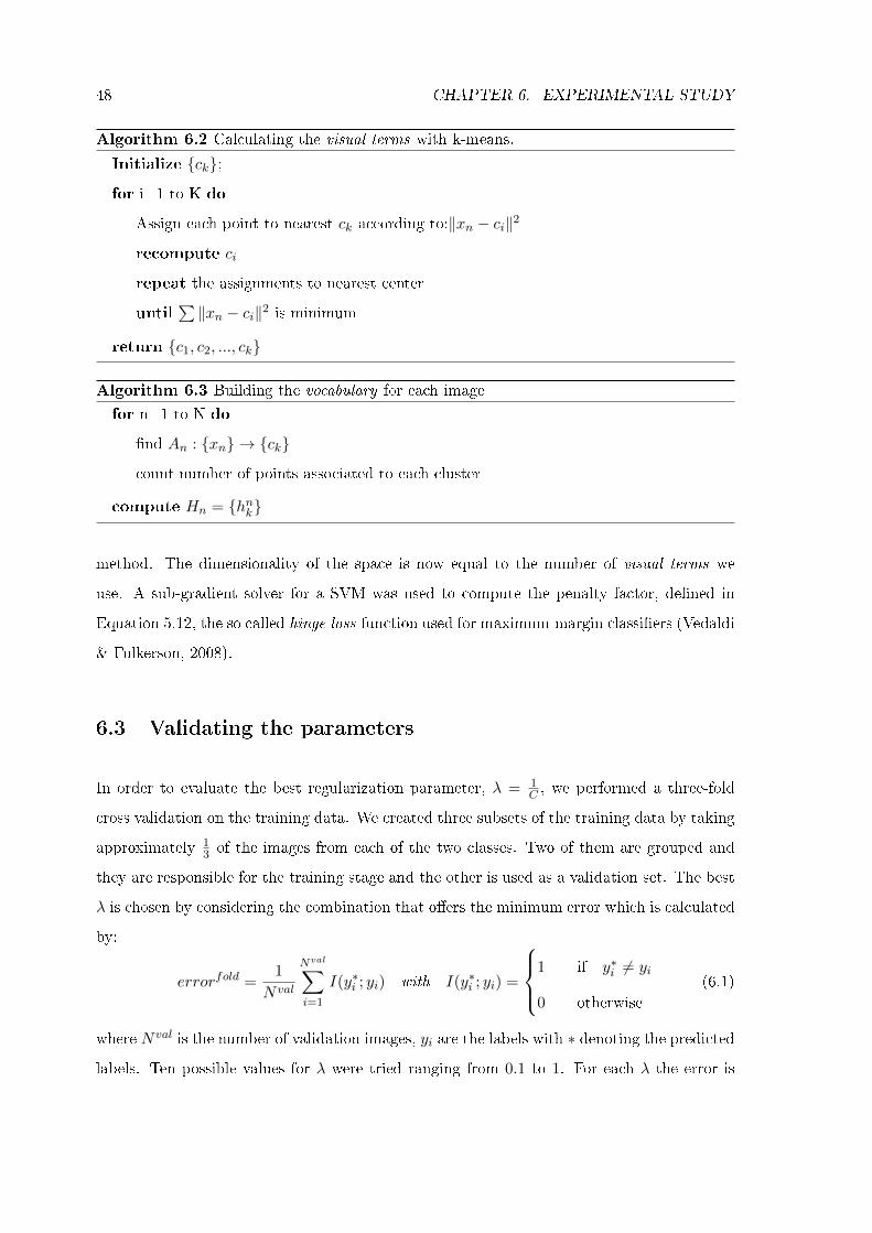
48 CHAPTER 6. EXPERIMENTAL STUDY
Algorithm 6.2 Calculating the visual terms with k-means.
Initialize {ck};for i=1 to K do
Assign each point to nearest ck according to:‖xn − ci‖2
recompute ci
repeat the assignments to nearest center
until∑ ‖xn − ci‖2 is minimum
return {c1, c2, ..., ck}
Algorithm 6.3 Building the vocabulary for each image
for n=1 to N do
�nd An : {xn} → {ck}count number of points associated to each cluster
compute Hn = {hnk}
method. The dimensionality of the space is now equal to the number of visual terms we
use. A sub-gradient solver for a SVM was used to compute the penalty factor, de�ned in
Equation 5.12, the so called hinge loss function used for maximum-margin classi�ers (Vedaldi
& Fulkerson, 2008).
6.3 Validating the parameters
In order to evaluate the best regularization parameter, λ = 1C , we performed a three-fold
cross validation on the training data. We created three subsets of the training data by taking
approximately 13 of the images from each of the two classes. Two of them are grouped and
they are responsible for the training stage and the other is used as a validation set. The best
λ is chosen by considering the combination that o�ers the minimum error which is calculated
by:
errorfold =1
Nval
Nval∑
i=1
I(y∗i ; yi) with I(y∗i ; yi) =
1 if y∗i 6= yi
0 otherwise
(6.1)
where Nval is the number of validation images, yi are the labels with ∗ denoting the predictedlabels. Ten possible values for λ were tried ranging from 0.1 to 1. For each λ the error is
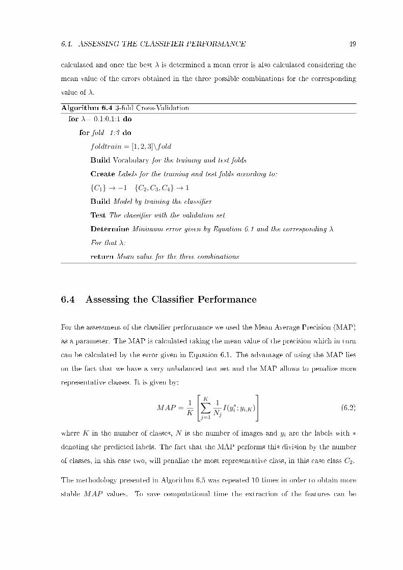
6.4. ASSESSING THE CLASSIFIER PERFORMANCE 49
calculated and once the best λ is determined a mean error is also calculated considering the
mean value of the errors obtained in the three possible combinations for the corresponding
value of λ.
Algorithm 6.4 3-fold Cross-Validation
for λ= 0.1:0.1:1 do
for fold=1:3 do
foldtrain = [1, 2, 3]\foldBuild Vocabulary for the training and test folds
Create Labels for the training and test folds according to:
{C1} → −1 {C2, C3, C4} → 1
Build Model by training the classi�er
Test The classi�er with the validation set
Determine Minimum error given by Equation 6.1 and the corresponding λ
For that λ:
return Mean value for the three combinations
6.4 Assessing the Classi�er Performance
For the assessment of the classi�er performance we used the Mean Average Precision (MAP)
as a parameter. The MAP is calculated taking the mean value of the precision which in turn
can be calculated by the error given in Equation 6.1. The advantage of using the MAP lies
on the fact that we have a very unbalanced test set and the MAP allows to penalize more
representative classes. It is given by:
MAP =1
K
K∑
j=1
1
NjI(y∗i ; yi,K)
(6.2)
where K in the number of classes, N is the number of images and yi are the labels with ∗denoting the predicted labels. The fact that the MAP performs this division by the number
of classes, in this case two, will penalize the most representative class, in this case class C2.
The methodology presented in Algorithm 6.5 was repeated 10 times in order to obtain more
stable MAP values. To save computational time the extraction of the features can be
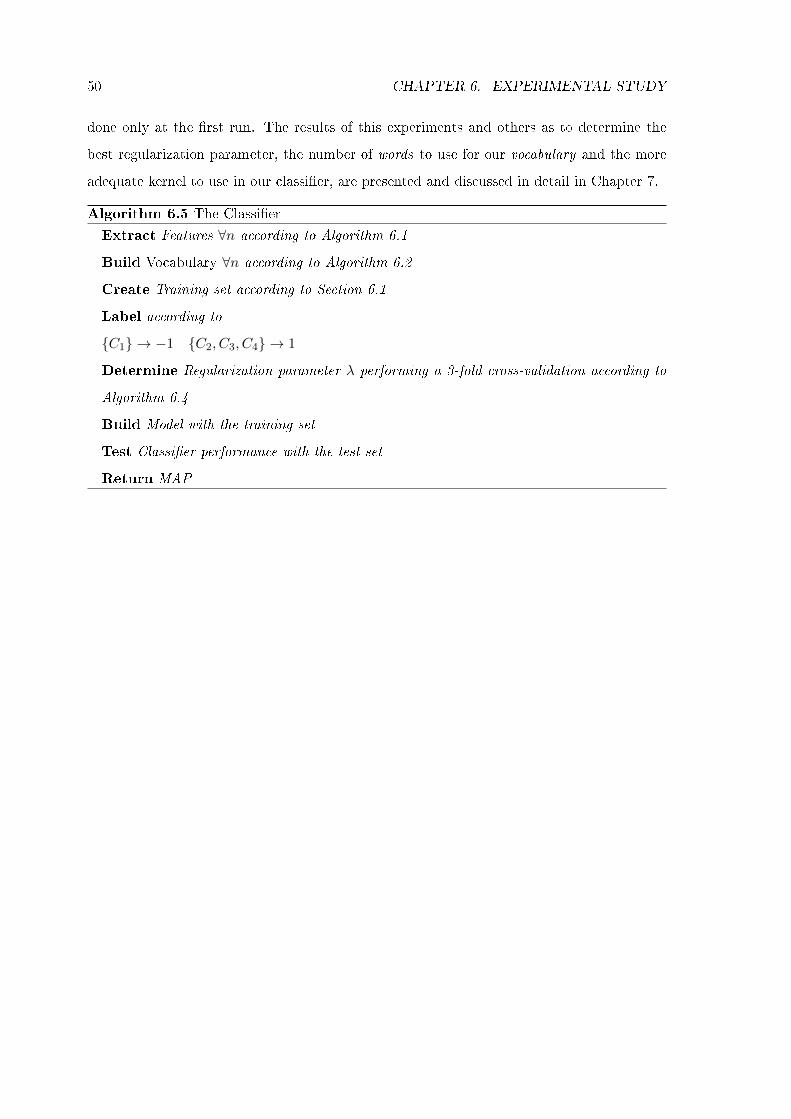
50 CHAPTER 6. EXPERIMENTAL STUDY
done only at the �rst run. The results of this experiments and others as to determine the
best regularization parameter, the number of words to use for our vocabulary and the more
adequate kernel to use in our classi�er, are presented and discussed in detail in Chapter 7.
Algorithm 6.5 The Classi�er
Extract Features ∀n according to Algorithm 6.1
Build Vocabulary ∀n according to Algorithm 6.2
Create Training set according to Section 6.1
Label according to
{C1} → −1 {C2, C3, C4} → 1
Determine Regularization parameter λ performing a 3-fold cross-validation according to
Algorithm 6.4
Build Model with the training set
Test Classi�er performance with the test set
Return MAP
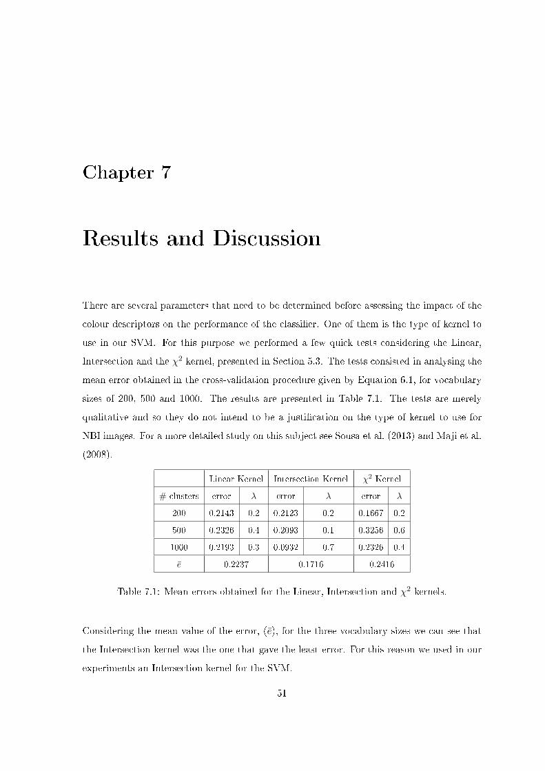
Chapter 7
Results and Discussion
There are several parameters that need to be determined before assessing the impact of the
colour descriptors on the performance of the classi�er. One of them is the type of kernel to
use in our SVM. For this purpose we performed a few quick tests considering the Linear,
Intersection and the χ2 kernel, presented in Section 5.3. The tests consisted in analysing the
mean error obtained in the cross-validation procedure given by Equation 6.1, for vocabulary
sizes of 200, 500 and 1000. The results are presented in Table 7.1. The tests are merely
qualitative and so they do not intend to be a justi�cation on the type of kernel to use for
NBI images. For a more detailed study on this subject see Sousa et al. (2013) and Maji et al.
(2008).
Linear Kernel Intersection Kernel χ2 Kernel
# clusters error λ error λ error λ
200 0.2143 0.2 0.2123 0.2 0.1667 0.2
500 0.2326 0.4 0.2093 0.1 0.3256 0.6
1000 0.2193 0.3 0.0932 0.7 0.2326 0.4
e 0.2237 0.1716 0.2416
Table 7.1: Mean errors obtained for the Linear, Intersection and χ2 kernels.
Considering the mean value of the error, (e), for the three vocabulary sizes we can see that
the Intersection kernel was the one that gave the least error. For this reason we used in our
experiments an Intersection kernel for the SVM.
51
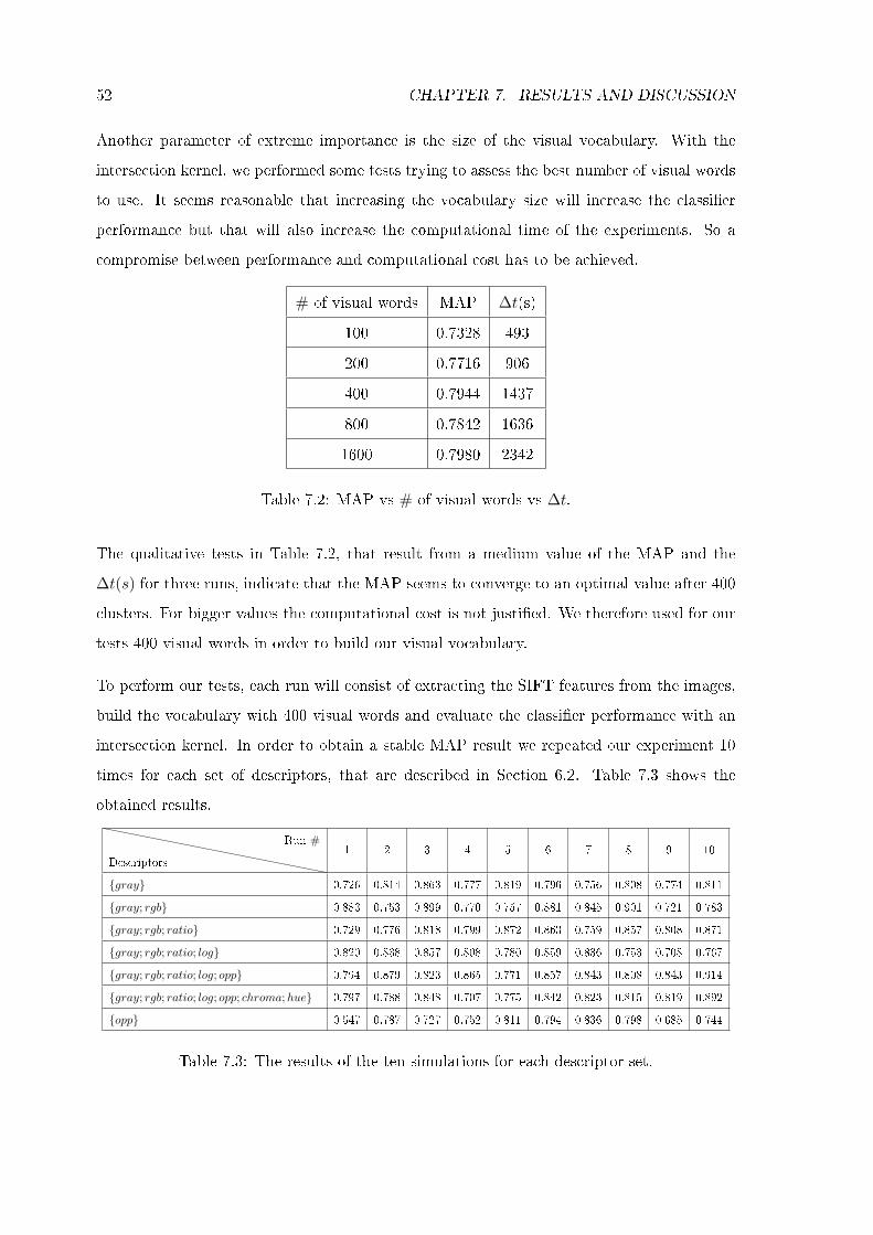
52 CHAPTER 7. RESULTS AND DISCUSSION
Another parameter of extreme importance is the size of the visual vocabulary. With the
intersection kernel, we performed some tests trying to assess the best number of visual words
to use. It seems reasonable that increasing the vocabulary size will increase the classi�er
performance but that will also increase the computational time of the experiments. So a
compromise between performance and computational cost has to be achieved.
# of visual words MAP ∆t(s)
100 0.7328 493
200 0.7716 906
400 0.7944 1437
800 0.7842 1636
1600 0.7980 2342
Table 7.2: MAP vs # of visual words vs ∆t.
The qualitative tests in Table 7.2, that result from a medium value of the MAP and the
∆t(s) for three runs, indicate that the MAP seems to converge to an optimal value after 400
clusters. For bigger values the computational cost is not justi�ed. We therefore used for our
tests 400 visual words in order to build our visual vocabulary.
To perform our tests, each run will consist of extracting the SIFT features from the images,
build the vocabulary with 400 visual words and evaluate the classi�er performance with an
intersection kernel. In order to obtain a stable MAP result we repeated our experiment 10
times for each set of descriptors, that are described in Section 6.2. Table 7.3 shows the
obtained results.
Descriptors
Run #1 2 3 4 5 6 7 8 9 10
{gray} 0.726 0.814 0.863 0.777 0.819 0.796 0.756 0.808 0.774 0.811
{gray; rgb} 0.883 0.753 0.899 0.770 0.757 0.881 0.845 0.901 0.721 0.783
{gray; rgb; ratio} 0.729 0.776 0.818 0.799 0.872 0.863 0.759 0.857 0.808 0.871
{gray; rgb; ratio; log} 0.820 0.838 0.857 0.808 0.780 0.859 0.836 0.753 0.708 0.767
{gray; rgb; ratio; log; opp} 0.794 0.879 0.823 0.865 0.771 0.857 0.843 0.808 0.843 0.914
{gray; rgb; ratio; log; opp; chroma;hue} 0.797 0.788 0.848 0.707 0.775 0.842 0.823 0.815 0.819 0.892
{opp} 0.547 0.787 0.727 0.752 0.811 0.794 0.836 0.798 0.685 0.744
Table 7.3: The results of the ten simulations for each descriptor set.
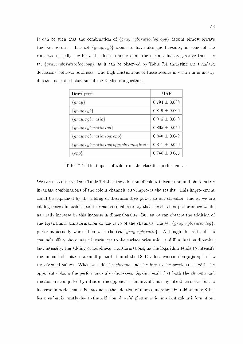
53
It can be seen that the combination of {gray; rgb; ratio; log; opp} attains almost always
the best results. The set {gray; rgb} seems to have also good results, in some of the
runs was actually the best, the �uctuations around the mean value are greater then the
set {gray; rgb; ratio; log; opp}, as it can be observed by Table 7.4 analysing the standard
deviations between both sets. The high �uctuations of these results in each run is mostly
due to stochastic behaviour of the K-Means algorithm.
Descriptors MAP
{gray} 0.794 ± 0.038
{gray; rgb} 0.819 ± 0.069
{gray; rgb; ratio} 0.815 ± 0.050
{gray; rgb; ratio; log} 0.805 ± 0.049
{gray; rgb; ratio; log; opp} 0.840 ± 0.042
{gray; rgb; ratio; log; opp; chroma;hue} 0.811 ± 0.049
{opp} 0.748 ± 0.083
Table 7.4: The impact of colour on the classi�er performance.
We can also observe from Table 7.4 that the addition of colour information and photometric
invariant combinations of the colour channels also improves the results. This improvement
could be explained by the adding of discriminative power to our classi�er, this is, we are
adding more dimensions, so it seems reasonable to say that the classi�er performance would
naturally increase by this increase in dimensionality. But as we can observe the addition of
the logarithmic transformation of the ratio of the channels, the set {gray; rgb; ratio; log},performs actually worse then with the set {gray; rgb; ratio}. Although the ratio of the
channels o�ers photometric invariances to the surface orientation and illumination direction
and intensity, the adding of non-linear transformations, as the logarithm tends to intensify
the amount of noise so a small perturbation of the RGB values causes a large jump in the
transformed values. When we add the chroma and the hue to the previous set with the
opponent colours the performance also decreases. Again, recall that both the chroma and
the hue are computed by ratios of the opponent colours and this may introduce noise. So the
increase in performance is not due to the addition of more dimensions by taking more SIFT
features but is mostly due to the addition of useful photometric invariant colour information.
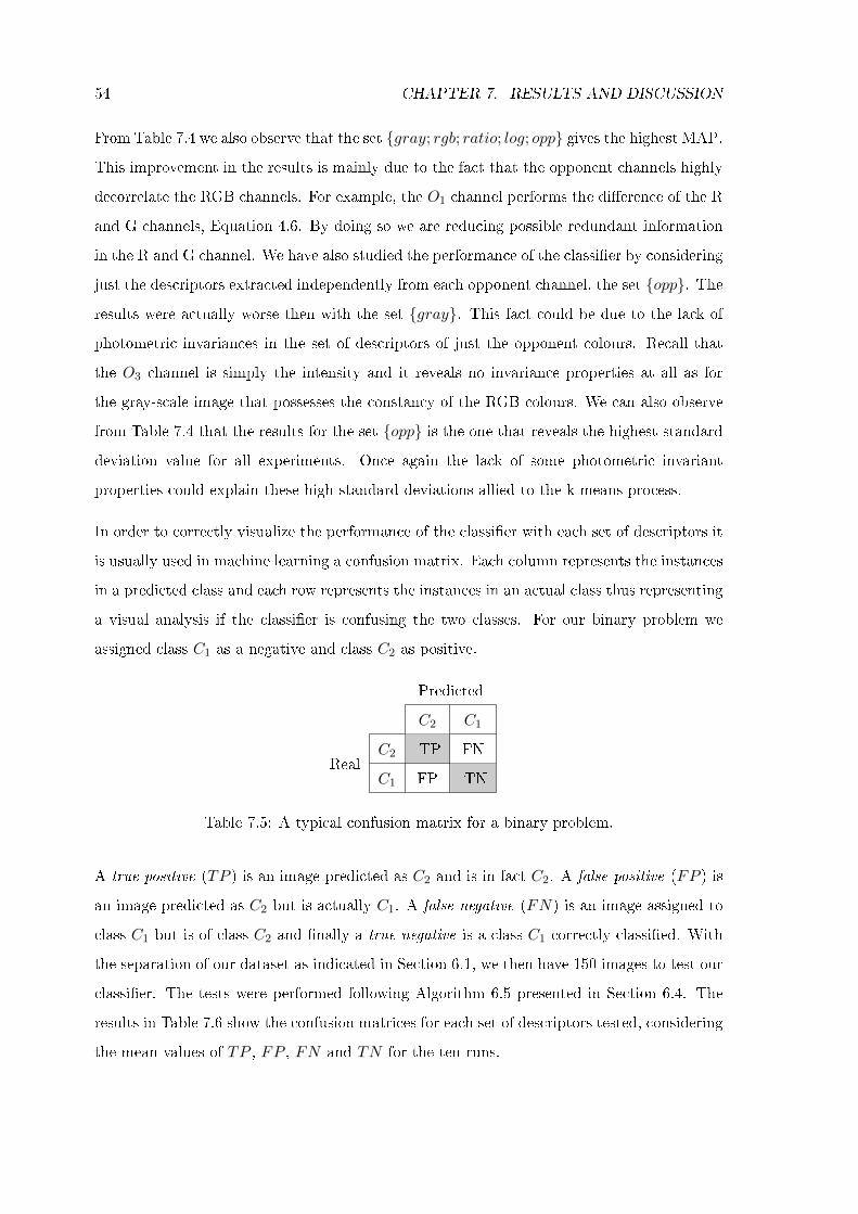
54 CHAPTER 7. RESULTS AND DISCUSSION
From Table 7.4 we also observe that the set {gray; rgb; ratio; log; opp} gives the highest MAP.
This improvement in the results is mainly due to the fact that the opponent channels highly
decorrelate the RGB channels. For example, the O1 channel performs the di�erence of the R
and G channels, Equation 4.6. By doing so we are reducing possible redundant information
in the R and G channel. We have also studied the performance of the classi�er by considering
just the descriptors extracted independently from each opponent channel, the set {opp}. Theresults were actually worse then with the set {gray}. This fact could be due to the lack of
photometric invariances in the set of descriptors of just the opponent colours. Recall that
the O3 channel is simply the intensity and it reveals no invariance properties at all as for
the gray-scale image that possesses the constancy of the RGB colours. We can also observe
from Table 7.4 that the results for the set {opp} is the one that reveals the highest standarddeviation value for all experiments. Once again the lack of some photometric invariant
properties could explain these high standard deviations allied to the k-means process.
In order to correctly visualize the performance of the classi�er with each set of descriptors it
is usually used in machine learning a confusion matrix. Each column represents the instances
in a predicted class and each row represents the instances in an actual class thus representing
a visual analysis if the classi�er is confusing the two classes. For our binary problem we
assigned class C1 as a negative and class C2 as positive.
Predicted
C2 C1
RealC2 TP FN
C1 FP TN
Table 7.5: A typical confusion matrix for a binary problem.
A true positive (TP ) is an image predicted as C2 and is in fact C2. A false positive (FP ) is
an image predicted as C2 but is actually C1. A false negative (FN) is an image assigned to
class C1 but is of class C2 and �nally a true negative is a class C1 correctly classi�ed. With
the separation of our dataset as indicated in Section 6.1, we then have 150 images to test our
classi�er. The tests were performed following Algorithm 6.5 presented in Section 6.4. The
results in Table 7.6 show the confusion matrices for each set of descriptors tested, considering
the mean values of TP , FP , FN and TN for the ten runs.
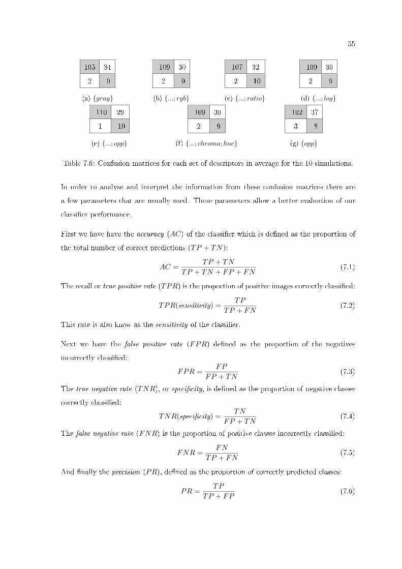
55
105 34
2 9
(a) {gray}
109 30
2 9
(b) {...; rgb}
107 32
2 10
(c) {...; ratio}
109 30
2 9
(d) {...; log}
110 29
1 10
(e) {...; opp}
109 30
2 9
(f) {...; chroma;hue}
102 37
3 8
(g) {opp}
Table 7.6: Confusion matrices for each set of descriptors in average for the 10 simulations.
In order to analyse and interpret the information from these confusion matrices there are
a few parameters that are usually used. These parameters allow a better evaluation of our
classi�er performance.
First we have have the accuracy (AC) of the classi�er which is de�ned as the proportion of
the total number of correct predictions (TP + TN):
AC =TP + TN
TP + TN + FP + FN(7.1)
The recall or true positive rate (TPR) is the proportion of positive images correctly classi�ed:
TPR(sensitivity) =TP
TP + FN(7.2)
This rate is also know as the sensitivity of the classi�er.
Next we have the false positive rate (FPR) de�ned as the proportion of the negatives
incorrectly classi�ed:
FPR =FP
FP + TN(7.3)
The true negative rate (TNR), or speci�city, is de�ned as the proportion of negative classes
correctly classi�ed:
TNR(speci�city) =TN
FP + TN(7.4)
The false negative rate (FNR) is the proportion of positive classes incorrectly classi�ed:
FNR =FN
TP + FN(7.5)
And �nally the precision (PR), de�ned as the proportion of correctly predicted classes:
PR =TP
TP + FP(7.6)
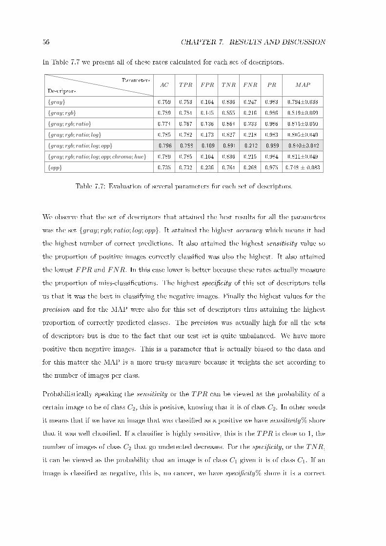
56 CHAPTER 7. RESULTS AND DISCUSSION
In Table 7.7 we present all of these rates calculated for each set of descriptors.
Descriptors
ParametersAC TPR FPR TNR FNR PR MAP
{gray} 0.759 0.753 0.164 0.836 0.247 0.983 0.794±0.038{gray; rgb} 0.789 0.784 0.145 0.855 0.216 0.986 0.819±0.069{gray; rgb; ratio} 0.774 0.767 0.136 0.864 0.233 0.986 0.815±0.050{gray; rgb; ratio; log} 0.785 0.782 0.173 0.827 0.218 0.983 0.805±0.049{gray; rgb; ratio; log; opp} 0.796 0.788 0.109 0.891 0.212 0.989 0.840±0.042{gray; rgb; ratio; log; opp; chroma;hue} 0.789 0.785 0.164 0.836 0.215 0.984 0.811±0.049{opp} 0.735 0.732 0.236 0.764 0.268 0.975 0.748 ± 0.083
Table 7.7: Evaluation of several parameters for each set of descriptors.
We observe that the set of descriptors that attained the best results for all the parameters
was the set {gray; rgb; ratio; log; opp}. It attained the highest accuracy which means it had
the highest number of correct predictions. It also attained the highest sensitivity value so
the proportion of positive images correctly classi�ed was also the highest. It also attained
the lowest FPR and FNR. In this case lower is better because these rates actually measure
the proportion of miss-classi�cations. The highest speci�city of this set of descriptors tells
us that it was the best in classifying the negative images. Finally the highest values for the
precision and for the MAP were also for this set of descriptors thus attaining the highest
proportion of correctly predicted classes. The precision was actually high for all the sets
of descriptors but is due to the fact that our test set is quite unbalanced. We have more
positive then negative images. This is a parameter that is actually biased to the data and
for this matter the MAP is a more trusty measure because it weights the set according to
the number of images per class.
Probabilistically speaking the sensitivity or the TPR can be viewed as the probability of a
certain image to be of class C2, this is positive, knowing that it is of class C2. In other words
it means that if we have an image that was classi�ed as a positive we have sensitivity% shore
that it was well classi�ed. If a classi�er is highly sensitive, this is the TPR is close to 1, the
number of images of class C2 that go undetected decreases. For the speci�city, or the TNR,
it can be viewed as the probability that an image is of class C1 given it is of class C1. If an
image is classi�ed as negative, this is, no cancer, we have speci�city% shore it is a correct
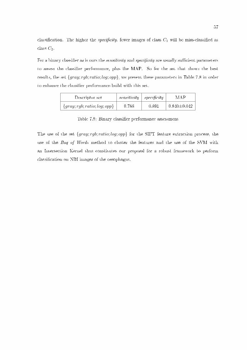
57
classi�cation. The higher the speci�city, fewer images of class C1 will be miss-classi�ed as
class C2.
For a binary classi�er as is ours the sensitivity and speci�city are usually su�cient parameters
to assess the classi�er performance, plus the MAP. So for the set that shows the best
results, the set {gray; rgb; ratio; log; opp}, we present these parameters in Table 7.8 in order
to enhance the classi�er performance build with this set.
Descriptor set sensitivity speci�city MAP
{gray; rgb; ratio; log; opp} 0.788 0.891 0.840±0.042
Table 7.8: Binary classi�er performance assessment
The use of the set {gray; rgb; ratio; log; opp} for the SIFT feature extraction process, the
use of the Bag of Words method to cluster the features and the use of the SVM with
an Intersection Kernel thus constitutes our proposal for a robust framework to perform
classi�cation on NBI images of the oesophagus.

58 CHAPTER 7. RESULTS AND DISCUSSION
Chapter 8
Conclusions and Future Works
In this thesis we proposed to develop a robust framework for the classi�cation of NBI images
of the oesophagus. We used a local descriptor densely sampled, DSIFT, to describe these
new images, performed the quanti�cation of these descriptors using the Bag of Words method
and used a SVM with an intersection kernel for the classi�cation.
The main goal was to study the impact of colour information to the base SIFT descriptor.
Adding this information was performed by following some physical properties of the images
itself and modulating them with the Dichromatic Re�ection Model that considers the tissue
as being composed by two layers. This modulation allows to rebuild the information on the
RGB channels and in turn obtain special photometric invariants. To the invariance of the
SIFT descriptor to scale, rotation and translation, we were able to add information invariant
to viewpoint, lighting geometry, specularities, surface orientation, illumination direction and
intensity and shading.
The obtained results show that to add information from the RGB channels independently,
the ratio of the RGB channels, the logarithmic of these ratios and the information from the
opponent colour gives the best results. With this set of local descriptors we attained a MAP
of 84.0%, a sensitivity of 78.8% and a speci�city of 89.1%. Its invariance properties allied to
the very special conditions that these images are acquired allow these descriptors to perform
very well. The addition of colour information improved the classi�er performance in about
5% comparing of course the referred set of local descriptors with the opponent colours to our
59
60 CHAPTER 8. CONCLUSIONS AND FUTURE WORKS
base gray descriptor. The fact that the opponent colour system highly decorrelates the RGB
channels explains this gain in the performance.
The work presented in this thesis can actually be extended and improved. Some of the
performed tests were merely qualitative as the tests performed to assess the more adequate
kernel to use in our SVM. The intersection kernel was chosen among the χ2 kernel and the
linear kernel performing only three experiments comparing the mean error for three possible
vocabulary sizes. With this is mind a more detailed study maybe performed in order to
attain the best kernel method to use. Another qualitative test performed was the size of the
vocabulary although the results do seem to justify the use of 400 visual terms to describe
these images for the sake of computational cost. Again maybe a more detailed study on this
subject may allow to determine a more e�ective size of the vocabulary. The use of these
qualitative tests is justi�ed by the main goal of this thesis that was to assess the classi�er
performance by adding colour information and so some parameters had to be �xed in order
to perform the tests.
Another topic worthy of interest is the process of the image formation in the NBI system
itself. A deeper knowledge of some of the characteristics of the NBI �lters that are used and
the process of rebuilding the image in the RGB monitor could provide valuable information
on the degree of correlation of the channels and possibly one could modulate the images
taking this information in consideration and obtain better results.
Appendix A
Abbreviations
CCD Charged-Coupled Device
NBI Narrow-band Imaging
RGB Red Green Blue
RORENO Registo Oncológico Regional do Norte
IPO-Porto Instituto Português de Oncologia do Porto Francisco Gentil
GERD Gastroesophageal Re�ux Disease
SCC Squamous Cell Carcinoma
BE Barrett's Oesophagus
SIFT Scale Invariant Feature Transform
DSIFT Dense SIFT
DoG Di�erence-of-Gaussian
SVM Support Vector Machine
MAP Mean Average Precision
CAD Computer Aided Diagnosis
DRM Dichromatic Re�ection Model
61

62 APPENDIX A. ABBREVIATIONS
Appendix B
Published Article at RecPad2013
63
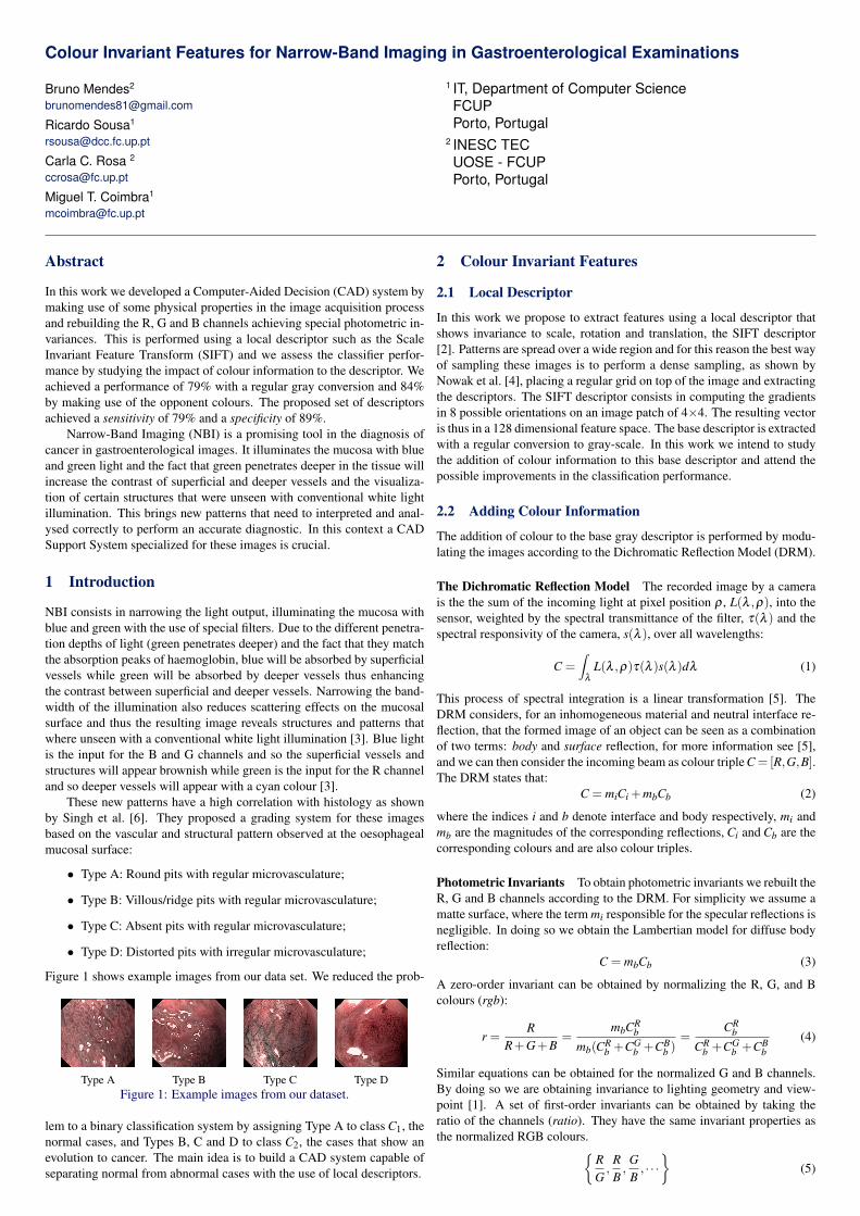
Colour Invariant Features for Narrow-Band Imaging in Gastroenterological Examinations
Bruno Mendes2
Ricardo Sousa1
Carla C. Rosa 2
Miguel T. Coimbra1
1 IT, Department of Computer ScienceFCUPPorto, Portugal
2 INESC TECUOSE - FCUPPorto, Portugal
Abstract
In this work we developed a Computer-Aided Decision (CAD) system bymaking use of some physical properties in the image acquisition processand rebuilding the R, G and B channels achieving special photometric in-variances. This is performed using a local descriptor such as the ScaleInvariant Feature Transform (SIFT) and we assess the classifier perfor-mance by studying the impact of colour information to the descriptor. Weachieved a performance of 79% with a regular gray conversion and 84%by making use of the opponent colours. The proposed set of descriptorsachieved a sensitivity of 79% and a specificity of 89%.
Narrow-Band Imaging (NBI) is a promising tool in the diagnosis ofcancer in gastroenterological images. It illuminates the mucosa with blueand green light and the fact that green penetrates deeper in the tissue willincrease the contrast of superficial and deeper vessels and the visualiza-tion of certain structures that were unseen with conventional white lightillumination. This brings new patterns that need to interpreted and anal-ysed correctly to perform an accurate diagnostic. In this context a CADSupport System specialized for these images is crucial.
1 Introduction
NBI consists in narrowing the light output, illuminating the mucosa withblue and green with the use of special filters. Due to the different penetra-tion depths of light (green penetrates deeper) and the fact that they matchthe absorption peaks of haemoglobin, blue will be absorbed by superficialvessels while green will be absorbed by deeper vessels thus enhancingthe contrast between superficial and deeper vessels. Narrowing the band-width of the illumination also reduces scattering effects on the mucosalsurface and thus the resulting image reveals structures and patterns thatwhere unseen with a conventional white light illumination [3]. Blue lightis the input for the B and G channels and so the superficial vessels andstructures will appear brownish while green is the input for the R channeland so deeper vessels will appear with a cyan colour [3].
These new patterns have a high correlation with histology as shownby Singh et al. [6]. They proposed a grading system for these imagesbased on the vascular and structural pattern observed at the oesophagealmucosal surface:
• Type A: Round pits with regular microvasculature;
• Type B: Villous/ridge pits with regular microvasculature;
• Type C: Absent pits with regular microvasculature;
• Type D: Distorted pits with irregular microvasculature;
Figure 1 shows example images from our data set. We reduced the prob-
Type A Type B Type C Type DFigure 1: Example images from our dataset.
lem to a binary classification system by assigning Type A to class C1, thenormal cases, and Types B, C and D to class C2, the cases that show anevolution to cancer. The main idea is to build a CAD system capable ofseparating normal from abnormal cases with the use of local descriptors.
2 Colour Invariant Features
2.1 Local Descriptor
In this work we propose to extract features using a local descriptor thatshows invariance to scale, rotation and translation, the SIFT descriptor[2]. Patterns are spread over a wide region and for this reason the best wayof sampling these images is to perform a dense sampling, as shown byNowak et al. [4], placing a regular grid on top of the image and extractingthe descriptors. The SIFT descriptor consists in computing the gradientsin 8 possible orientations on an image patch of 4×4. The resulting vectoris thus in a 128 dimensional feature space. The base descriptor is extractedwith a regular conversion to gray-scale. In this work we intend to studythe addition of colour information to this base descriptor and attend thepossible improvements in the classification performance.
2.2 Adding Colour Information
The addition of colour to the base gray descriptor is performed by modu-lating the images according to the Dichromatic Reflection Model (DRM).
The Dichromatic Reflection Model The recorded image by a camerais the the sum of the incoming light at pixel position ρ , L(λ ,ρ), into thesensor, weighted by the spectral transmittance of the filter, τ(λ ) and thespectral responsivity of the camera, s(λ ), over all wavelengths:
C =∫
λL(λ ,ρ)τ(λ )s(λ )dλ (1)
This process of spectral integration is a linear transformation [5]. TheDRM considers, for an inhomogeneous material and neutral interface re-flection, that the formed image of an object can be seen as a combinationof two terms: body and surface reflection, for more information see [5],and we can then consider the incoming beam as colour triple C = [R,G,B].The DRM states that:
C = miCi +mbCb (2)
where the indices i and b denote interface and body respectively, mi andmb are the magnitudes of the corresponding reflections, Ci and Cb are thecorresponding colours and are also colour triples.
Photometric Invariants To obtain photometric invariants we rebuilt theR, G and B channels according to the DRM. For simplicity we assume amatte surface, where the term mi responsible for the specular reflections isnegligible. In doing so we obtain the Lambertian model for diffuse bodyreflection:
C = mbCb (3)
A zero-order invariant can be obtained by normalizing the R, G, and Bcolours (rgb):
r =R
R+G+B=
mbCRb
mb(CRb +CG
b +CBb )
=CR
b
CRb +CG
b +CBb
(4)
Similar equations can be obtained for the normalized G and B channels.By doing so we are obtaining invariance to lighting geometry and view-point [1]. A set of first-order invariants can be obtained by taking theratio of the channels (ratio). They have the same invariant properties asthe normalized RGB colours.
{RG,
RB,
GB, · · ·}
(5)
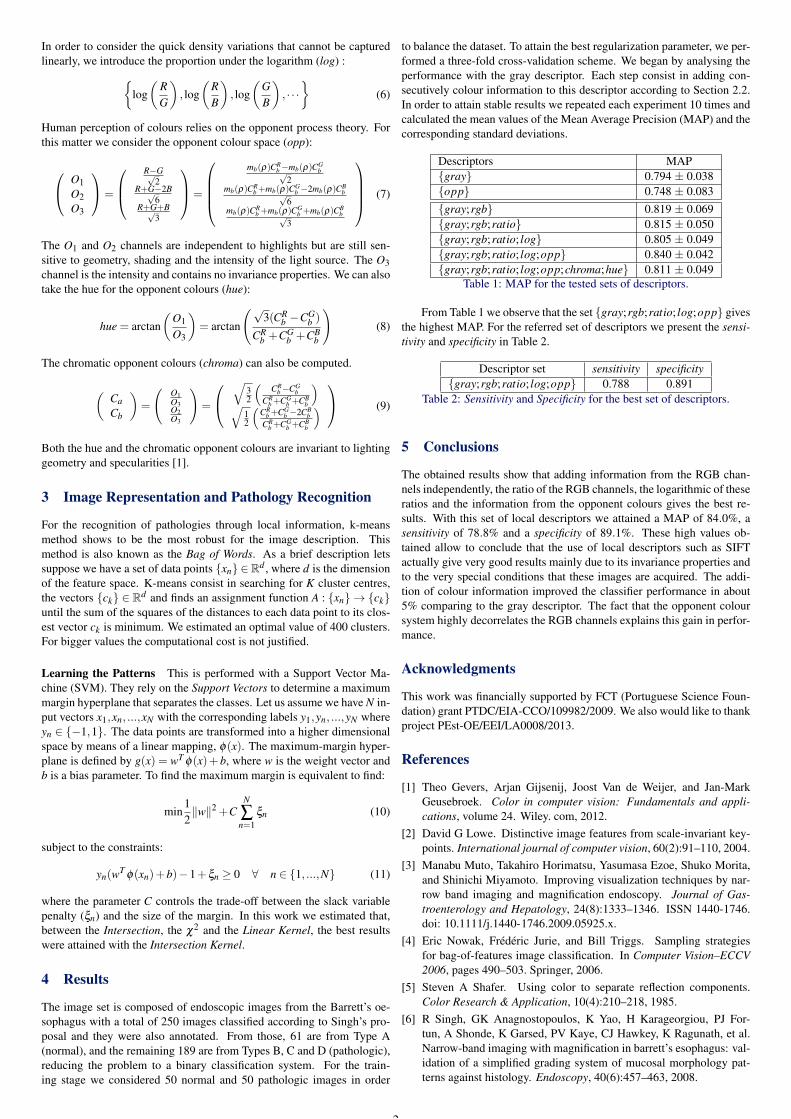
In order to consider the quick density variations that cannot be capturedlinearly, we introduce the proportion under the logarithm (log) :
{log(
RG
), log
(RB
), log
(GB
), · · ·}
(6)
Human perception of colours relies on the opponent process theory. Forthis matter we consider the opponent colour space (opp):
O1O2O3
=
R−G√2
R+G−2B√6
R+G+B√3
=
mb(ρ)CRb−mb(ρ)CG
b√2
mb(ρ)CRb +mb(ρ)CG
b −2mb(ρ)CBb√
6mb(ρ)CR
b +mb(ρ)CGb +mb(ρ)CB
b√3
(7)
The O1 and O2 channels are independent to highlights but are still sen-sitive to geometry, shading and the intensity of the light source. The O3channel is the intensity and contains no invariance properties. We can alsotake the hue for the opponent colours (hue):
hue = arctan(
O1
O3
)= arctan
(√3(CR
b −CGb )
CRb +CG
b +CBb
)(8)
The chromatic opponent colours (chroma) can also be computed.
(CaCb
)=
(O1O3O2O3
)=
√32
(CR
b−CGb
CRb +CG
b +CBb
)√
12
(CR
b +CGb −2CB
bCR
b +CGb +CB
b
) (9)
Both the hue and the chromatic opponent colours are invariant to lightinggeometry and specularities [1].
3 Image Representation and Pathology Recognition
For the recognition of pathologies through local information, k-meansmethod shows to be the most robust for the image description. Thismethod is also known as the Bag of Words. As a brief description letssuppose we have a set of data points {xn} ∈Rd , where d is the dimensionof the feature space. K-means consist in searching for K cluster centres,the vectors {ck} ∈ Rd and finds an assignment function A : {xn} → {ck}until the sum of the squares of the distances to each data point to its clos-est vector ck is minimum. We estimated an optimal value of 400 clusters.For bigger values the computational cost is not justified.
Learning the Patterns This is performed with a Support Vector Ma-chine (SVM). They rely on the Support Vectors to determine a maximummargin hyperplane that separates the classes. Let us assume we have N in-put vectors x1,xn, ...,xN with the corresponding labels y1,yn, ...,yN whereyn ∈ {−1,1}. The data points are transformed into a higher dimensionalspace by means of a linear mapping, φ(x). The maximum-margin hyper-plane is defined by g(x) = wT φ(x)+b, where w is the weight vector andb is a bias parameter. To find the maximum margin is equivalent to find:
min12‖w‖2 +C
N
∑n=1
ξn (10)
subject to the constraints:
yn(wT φ(xn)+b)−1+ξn ≥ 0 ∀ n ∈ {1, ...,N} (11)
where the parameter C controls the trade-off between the slack variablepenalty (ξn) and the size of the margin. In this work we estimated that,between the Intersection, the χ2 and the Linear Kernel, the best resultswere attained with the Intersection Kernel.
4 Results
The image set is composed of endoscopic images from the Barrett’s oe-sophagus with a total of 250 images classified according to Singh’s pro-posal and they were also annotated. From those, 61 are from Type A(normal), and the remaining 189 are from Types B, C and D (pathologic),reducing the problem to a binary classification system. For the train-ing stage we considered 50 normal and 50 pathologic images in order
to balance the dataset. To attain the best regularization parameter, we per-formed a three-fold cross-validation scheme. We began by analysing theperformance with the gray descriptor. Each step consist in adding con-secutively colour information to this descriptor according to Section 2.2.In order to attain stable results we repeated each experiment 10 times andcalculated the mean values of the Mean Average Precision (MAP) and thecorresponding standard deviations.
Descriptors MAP{gray} 0.794 ± 0.038{opp} 0.748 ± 0.083{gray;rgb} 0.819 ± 0.069{gray;rgb;ratio} 0.815 ± 0.050{gray;rgb;ratio; log} 0.805 ± 0.049{gray;rgb;ratio; log;opp} 0.840 ± 0.042{gray;rgb;ratio; log;opp;chroma;hue} 0.811 ± 0.049
Table 1: MAP for the tested sets of descriptors.
From Table 1 we observe that the set {gray;rgb;ratio; log;opp} givesthe highest MAP. For the referred set of descriptors we present the sensi-tivity and specificity in Table 2.
Descriptor set sensitivity specificity{gray;rgb;ratio; log;opp} 0.788 0.891
Table 2: Sensitivity and Specificity for the best set of descriptors.
5 Conclusions
The obtained results show that adding information from the RGB chan-nels independently, the ratio of the RGB channels, the logarithmic of theseratios and the information from the opponent colours gives the best re-sults. With this set of local descriptors we attained a MAP of 84.0%, asensitivity of 78.8% and a specificity of 89.1%. These high values ob-tained allow to conclude that the use of local descriptors such as SIFTactually give very good results mainly due to its invariance properties andto the very special conditions that these images are acquired. The addi-tion of colour information improved the classifier performance in about5% comparing to the gray descriptor. The fact that the opponent coloursystem highly decorrelates the RGB channels explains this gain in perfor-mance.
Acknowledgments
This work was financially supported by FCT (Portuguese Science Foun-dation) grant PTDC/EIA-CCO/109982/2009. We also would like to thankproject PEst-OE/EEI/LA0008/2013.
References
[1] Theo Gevers, Arjan Gijsenij, Joost Van de Weijer, and Jan-MarkGeusebroek. Color in computer vision: Fundamentals and appli-cations, volume 24. Wiley. com, 2012.
[2] David G Lowe. Distinctive image features from scale-invariant key-points. International journal of computer vision, 60(2):91–110, 2004.
[3] Manabu Muto, Takahiro Horimatsu, Yasumasa Ezoe, Shuko Morita,and Shinichi Miyamoto. Improving visualization techniques by nar-row band imaging and magnification endoscopy. Journal of Gas-troenterology and Hepatology, 24(8):1333–1346. ISSN 1440-1746.doi: 10.1111/j.1440-1746.2009.05925.x.
[4] Eric Nowak, Frédéric Jurie, and Bill Triggs. Sampling strategiesfor bag-of-features image classification. In Computer Vision–ECCV2006, pages 490–503. Springer, 2006.
[5] Steven A Shafer. Using color to separate reflection components.Color Research & Application, 10(4):210–218, 1985.
[6] R Singh, GK Anagnostopoulos, K Yao, H Karageorgiou, PJ For-tun, A Shonde, K Garsed, PV Kaye, CJ Hawkey, K Ragunath, et al.Narrow-band imaging with magnification in barrett’s esophagus: val-idation of a simplified grading system of mucosal morphology pat-terns against histology. Endoscopy, 40(6):457–463, 2008.
2

66 APPENDIX B. PUBLISHED ARTICLE AT RECPAD2013
References
Bashkatov, A., Genina, E., Kochubey, V., & Tuchin, V. (2005). Optical properties of human
skin, subcutaneous and mucous tissues in the wavelength range from 400 to 2000 nm.
Journal of Physics D: Applied Physics, 38(15), 2543.
Bishop, C. M. & Nasrabadi, N. M. (2006). Pattern recognition and machine learning,
volume 1. springer New York.
Bryan, R. T., Billingham, L. J., & Wallace, D. M. A. (2008). Narrow-band imaging �exible
cystoscopy in the detection of recurrent urothelial cancer of the bladder. BJU International,
101(6), 702�706.
Coimbra, M. & Cunha, J. (2006). Mpeg-7 visual descriptors 8212; contributions for
automated feature extraction in capsule endoscopy. Circuits and Systems for Video
Technology, IEEE Transactions on, 16(5), 628 � 637.
Coimbra, M., Riaz, F., Areia, M., Silva, F., & Dinis-Ribeiro, M. (2010). Segmentation for
classi�cation of gastroenterology images. In Engineering in Medicine and Biology Society
(EMBC), 2010 Annual International Conference of the IEEE (pp. 4744 �4747).
Ganz, M., Yang, X., & Slabaugh, G. (2012). Automatic segmentation of polyps in
colonoscopic narrow-band imaging data. Biomedical Engineering, IEEE Transactions on,
59(8), 2144 �2151.
Gevers, T., Gijsenij, A., Van de Weijer, J., & Geusebroek, J.-M. (2012). Color in computer
vision: Fundamentals and applications, volume 24. Wiley. com.
Hecht, E. (1998). Optics. Addison-Wesley, 4th edition.
67
68 REFERENCES
Jobe, B. A., Thomas, C. R., & Hunter, J. G. (2009). Esophageal cancer: principles and
practice. Demos Medical Publishing.
Karargyris, A. & Bourbakis, N. (2009). Identi�cation of polyps in wireless capsule endoscopy
videos using log gabor �lters. In Life Science Systems and Applications Workshop, 2009.
LiSSA 2009. IEEE/NIH (pp. 143 �147).
Karkanis, S., Iakovidis, D., Karras, D., & Maroulis, D. (2001). Detection of lesions in
endoscopic video using textural descriptors on wavelet domain supported by arti�cial
neural network architectures. In Image Processing, 2001. Proceedings. 2001 International
Conference on, volume 2 (pp. 833 �836 vol.2).
Karkanis, S., Iakovidis, D., Maroulis, D., Karras, D., & Tzivras, M. (2003). Computer-aided
tumor detection in endoscopic video using color wavelet features. Information Technology
in Biomedicine, IEEE Transactions on, 7(3), 141 �152.
Khademi, A. & Krishnan, S. (2007). Multiresolution analysis and classi�cation of small bowel
medical images. In Engineering in Medicine and Biology Society, 2007. EMBS 2007. 29th
Annual International Conference of the IEEE (pp. 4524 �4527).
Kwitt, R. & Uhl, A. (2007). Modeling the marginal distributions of complex wavelet
coe�cient magnitudes for the classi�cation of zoom-endoscopy images. In Computer
Vision, 2007. ICCV 2007. IEEE 11th International Conference on (pp. 1 �8).
Liedlgruber, M. & Uhl, A. (2011). Computer-aided decision support systems for endoscopy
in the gastrointestinal tract: A review. Biomedical Engineering, IEEE Reviews in, 4, 73
�88.
Lima, C. S., Barbosa, D., Ramos, J., Tavares, A., Monteiro, L., & Carvalho, L. (2008).
Classi�cation of endoscopic capsule images by using color wavelet features, higher order
statistics and radial basis functions. In Engineering in Medicine and Biology Society, 2008.
EMBS 2008. 30th Annual International Conference of the IEEE (pp. 1242 �1245).
Lowe, D. G. (1999). Object recognition from local scale-invariant features. In Computer
vision, 1999. The proceedings of the seventh IEEE international conference on, volume 2
(pp. 1150�1157).: Ieee.
REFERENCES 69
Lowe, D. G. (2004). Distinctive image features from scale-invariant keypoints. International
journal of computer vision, 60(2), 91�110.
Maji, S., Berg, A. C., & Malik, J. (2008). Classi�cation using intersection kernel support
vector machines is e�cient. In Computer Vision and Pattern Recognition, 2008. CVPR
2008. IEEE Conference on (pp. 1�8).: IEEE.
Muto, M., Horimatsu, T., Ezoe, Y., Morita, S., & Miyamoto, S. (2009). Improving
visualization techniques by narrow band imaging and magni�cation endoscopy. Journal of
Gastroenterology and Hepatology, 24(8), 1333�1346.
Niemz, M. (2007). Laser-tissue interactions: fundamentals and applications. Springer.
Nowak, E., Jurie, F., & Triggs, B. (2006). Sampling strategies for bag-of-features image
classi�cation. In Computer Vision�ECCV 2006 (pp. 490�503). Springer.
Poh, C. K., Htwe, T. M., Li, L., Shen, W., Liu, J., Lim, J. H., Chan, K. L., & Tan, P. C.
(2010). Multi-level local feature classi�cation for bleeding detection in wireless capsule
endoscopy images. In Cybernetics and Intelligent Systems (CIS), 2010 IEEE Conference
on (pp. 76 �81).
Shafer, S. A. (1985). Using color to separate re�ection components. Color Research &
Application, 10(4), 210�218.
Shawe-Taylor, J. & Cristianini, N. (2004). Kernel methods for pattern analysis. Cambridge
university press.
Singh, R., Anagnostopoulos, G., Yao, K., Karageorgiou, H., Fortun, P., Shonde, A., Garsed,
K., Kaye, P., Hawkey, C., Ragunath, K., et al. (2008). Narrow-band imaging with
magni�cation in barrett's esophagus: validation of a simpli�ed grading system of mucosal
morphology patterns against histology. Endoscopy, 40(6), 457�463.
Sousa, A., Dinis-Ribeiro, M., Areia, M., & Coimbra, M. (2009). Identifying cancer regions
in vital-stained magni�cation endoscopy images using adapted color histograms. In Image
Processing (ICIP), 2009 16th IEEE International Conference on (pp. 681 �684).
70 REFERENCES
Sousa, R., Coimbra, M. T., Ribeiro, M.-D., & Pimentel-Nunes, P. (2013). Impact of svm
multiclass decomposition rules for recognition of cancer in gastroenterology images. In
CBMS. ACCEPTED.
Stehle, T., Auer, R., Gross, S., Behrens, A., Wul�, J., Aach, T., Winograd, R., Trautwein,
C., & Tischendorf, J. (2009). Classi�cation of colon polyps in NBI endoscopy using
vascularization features. In N. Karssemeijer & M. L. Giger (Eds.), Medical Imaging 2009:
Computer-Aided Diagnosis, volume 7260 Orlando, USA: SPIE.
Van De Weijer, J., Gevers, T., & Geusebroek, J.-M. (2005). Edge and corner detection
by photometric quasi-invariants. Pattern Analysis and Machine Intelligence, IEEE
Transactions on, 27(4), 625�630.
Vedaldi, A. & Fulkerson, B. (2008). VLFeat: An open and portable library of computer
vision algorithms. http://www.vlfeat.org/.


![3RUWR $OHJUH 6HJXQGD IHLUD GH 'H]HPEUR GH 'LiULR … › upload › arquivos › ...(vvhqfldlv uxd wudedokdgruhv 7hohwudedokr 3uhvhqfldo uhvwulwr 3uhvhqfldo uhvwulwr 7hohqwuhjd 3hjxh](https://img.pdfslide.us/doc/110x75/60cf294c6ceb83431d5b701e/3ruwr-ohjuh-6hjxqgd-ihlud-gh-hhpeur-gh-liulr-a-upload-a-arquivos-a-.jpg)


![]HU 'DWH BBBBBBBBB](https://img.pdfslide.us/doc/110x75/621722a76001946ed937722f/hu-dwh-bbbbbbbbb.jpg)