HRE: The Home Range Extension for ArcView™ (Beta Test Version 0.9, July 1998)

User's Manual

Arthur R. Rodgers and Angus P. Carr

07/03/02 i

Table of Contents Introduction .................................................................................................................................................. 1

What is "Home Range Analysis"? ....................................................................................................... 1

Why use the ArcView GIS? ................................................................................................................ 2

Techniques available in the HRE......................................................................................................... 2

Minimum Convex Polygons..................................................................................................... 3

Kernel Methods ........................................................................................................................ 3

Some ArcView basics ..................................................................................................................................... 5

Projects ................................................................................................................................................ 5

Views .................................................................................................................................................. 6

Themes ................................................................................................................................................ 6

Tables .................................................................................................................................................. 7

Queries................................................................................................................................................. 7

Temporary Files................................................................................................................................... 7

Viewing and Saving Results ................................................................................................................ 8

Installing the Home Range Extension............................................................................................................. 9

Adding the Extension to a Project ....................................................................................................... 9

Saving your Project ............................................................................................................................. 9

Importing Fix Data........................................................................................................................................ 10

LOTEK .DAT files ............................................................................................................................ 10

Argos DCLS Files ............................................................................................................................. 11

Text Files and dBASE Files .............................................................................................................. 12

ARC/INFO Coverages....................................................................................................................... 13

Other Information .............................................................................................................................. 13

Editing Fix Data............................................................................................................................................ 14

Removing individual points............................................................................................................... 14

Removing Duplicates ........................................................................................................................ 14

07/03/02 ii

Merging Themes................................................................................................................................ 14

Exploratory ................................................................................................................................................ 15

“Moose On A Leash” ........................................................................................................................ 15

Analyzing Fix Data ....................................................................................................................................... 16

Calculating Interfix Times and Distances.......................................................................................... 16

Generating Minimum Convex Polygons ........................................................................................... 17

100% ...................................................................................................................................... 17

Fixed Amean .......................................................................................................................... 17

Floating Amean ...................................................................................................................... 17

Area Added ............................................................................................................................ 18

Median.................................................................................................................................... 18

User Point............................................................................................................................... 18

Generating Kernel Polygons ......................................................................................................................... 18

Independence of Observations........................................................................................................... 19

Choice of Smoothing Parameter ........................................................................................................ 19

Fixed/Adaptive Smoothing................................................................................................................ 22

Volume/Density Contouring.............................................................................................................. 22

Choice of Resolution ......................................................................................................................... 23

Analyzing Habitat Use.................................................................................................................................. 24

Overlap Analysis ............................................................................................................................... 24

Combining Themes............................................................................................................................ 25

References ................................................................................................................................................ 26

07/03/02 1

Introduction This manual is intended to accompany the Home Range Extension (HRE) for the ArcView®

Geographic Information System (GIS). The manual has been written for novice GIS users who already

understand basic wildlife telemetry issues and who are familiar with the concept of a “home range”.

The HRE contains software that extends ArcView to analyze home ranges of animals. This is

accomplished within a GIS, which provides a common and relatively familiar interface for analyses

performed on the fixes and on the home range polygons. The user should be able to perform all the

analyses of their point data within ArcView and the HRE.

What is "Home Range Analysis"?

Field studies of animals commonly record the locations where individuals are observed. In many

cases these point data, often referred to as "fixes", are determined by radio telemetry. These data may be

used in both "basic" and "applied" contexts. The information may be used to test basic hypotheses

concerning animal behaviour, resource use, population distribution, or interactions among individuals and

populations. Location data may also be used in conservation and management of species. The problem for

researchers is to determine which data points are relevant to their needs and how to best summarize the

information.

Researchers are rarely interested in every point that is visited, or the entire area used by an animal

during its lifetime. Instead, they focus on the animal's "home range", which is defined as "…that area

traversed by the individual in its normal activities of food gathering, mating, and caring for young.

Occasional sallies outside the area, perhaps exploratory in nature, should not be considered as in part of the

home range." (Burt 1943). Thus, in its simplest form, "home range analysis" involves the delineation of the

area in which an animal conducts its "normal" activities. This can often be accomplished through subjective

evaluation. To maintain scientific integrity (i.e., repeatability) or for comparisons with other studies,

however, objective criteria must be used to select movements that are "normal" (White and Garrott 1990).

The obvious difficulty is in the definition of what should be considered "normal". Because of this difficulty,

there has been a proliferation of home range analysis models.

Depending on the general treatment of point location estimates, home range analysis models can

be classified into four fundamentally different approaches; minimum convex polygons, bivariate normal

models (Jennrich-Turner estimator, weighted bivariate normal estimator, multiple ellipses, Dunn

estimator), nonparametric models (grid cell counts, Fourier series smoothing, harmonic mean), and

contouring models (peeled polygons, kernel methods, hierarchical incremental cluster analysis). All of

these methods can be used to estimate areas occupied by animals, but some have been developed to

specifically elucidate characteristics of home range shape (e.g., bivariate normal models) or structure (e.g.,

contouring models). If home range size is combined with information about home range shape, then it is

possible to estimate resources available to individuals in a population. Consideration of home range shape

07/03/02 2

may also allow identification of potential interactions among individuals. Analytical models developed to

examine home range structure may be useful in the identification of areas within home ranges that are used

by individuals for specific purposes such as nest sites or food caches. However, home range analysis may

involve more than just estimating the characteristics of areas occupied by animals. Researchers often want

to know about the distances, headings, times and speed of animal movements between locations. They may

also want to assess interactions of animals based on areas of overlap among home ranges or distances

between individuals at a particular point in time. Thus, home range analysis comprises a wide variety of

techniques and approaches. Most of these methods and their limitations have been reviewed by Harris et al.

(1990) and White and Garrott (1990).

Why use the ArcView GIS?

Just as there has been a proliferation of home range analysis models, there has been a proliferation

of home range analysis software. Characteristics of many software programs used to estimate animal home

ranges are summarized by Larkin and Halkin (1994) and Lawson and Rodgers (1997). Most of these are

older DOS-based programs with a cumbersome interface that requires batch files or data manipulation to be

carried out with text editors or database programs. This results in a multi-stage procedure that is time-

consuming and has the potential for error at each step in the process. Because of their age, most of the

existing programs do not include some of the more recent home range models (e.g., kernel methods). Many

of these programs do not allow export of home range polygons to a GIS for habitat analyses. Of those that

do, most are limited to fewer than 1,000 animal locations in the home range analysis. Although these

limitations may be acceptable to studies involving conventional radio-tracking of animals, automated

equipment such as recently developed GPS-based telemetry systems (Rodgers et al. 1996) can easily

generate enormous quantities of data that cannot be entirely analyzed by these previous software programs.

The ability to use large data sets and carry out all required home range analyses within a single software

environment was our primary reason for developing the HRE within the ArcView GIS.

Techniques available in the HRE

The HRE currently includes 2 home range analysis models: minimum convex polygons (MCPs)

and kernel methods. Although they have been severely criticized, MCPs have been included because they

are easy to compare among studies and they are the most frequently used (Harris et al. 1990, White and

Garrott 1990). Whereas MCPs do not indicate how intensively different parts of an animal's range are used,

kernel methods allow determination of centres of activity (Worton 1989, 1995, Seaman and Powell 1996).

Because different computer software programs may produce large differences in home range estimates

based on these models (Lawson and Rodgers 1997), we have attempted to provide all of the options offered

in earlier programs for calculation of the estimators and values input for various parameters.

07/03/02 3

Minimum Convex Polygons

Minimum convex polygons (MCPs) are constructed by connecting the peripheral points of a group

of points, such that external angles are greater than 180° (Mohr 1947). "Percent" minimum convex

polygons (%MCPs) (Michener 1979), sometimes referred to as "probability polygons" (Kenward 1987),

"restricted polygons" (Harris et al. 1990), or "mononuclear peeled polygons" (Kenward and Hodder1996),

can be generated for a subset of fixes using one of several percentage selection methods available in the

HRE. These methods include both the exclusion of points from a calculated (e.g., mean) or user-specified

(e.g., nest site) location, and an ordering criterion based on the amount of area each point contributes to the

%MCP (White and Garrott 1990).

Kernel Methods

Kernel analysis is a nonparametric statistical method for estimating probability densities from a set

of points. Kernel density estimation is well understood by statisticians, having been well explored since the

1950's. However, kernel methods have only been used in home range analysis for less than a decade

(Worton 1989). In the context of home range analysis these methods describe the probability of finding an

animal in any one place. The method begins by centring a bivariate probability density function with unit

volume (i.e., the "kernel") over each recorded point. A regular grid is then superimposed on the data and a

density estimate is calculated at each grid intersection. The density estimate at each intersection is

essentially the average of the kernel ordinates at that point. A bivariate kernel density estimator (i.e., a

"utilization distribution") is then calculated over the entire grid using the density estimates at each grid

intersection. The resulting kernel density estimator will thus have relatively large values in areas with many

observations and low values in areas with few. Home range estimates are derived by drawing contour lines

(i.e., isopleths) based on the volume of the curve under the utilization distribution. Alternatively, isopleths

can be drawn that connect regions of equal kernel density. In either case, the isopleths define home range

polygons whose areas can be calculated.

The HRE includes both fixed and adaptive kernel methods. The kernel function used in the HRE is

the standard bivariate normal (i.e., Gaussian) curve. Other kernel functions are described in Silverman

(1986), but have not been implemented. The choice of an appropriate "smoothing factor" (i.e.,

"bandwidth") is much more important than the choice of a kernel (Worton 1989) and there should be little

difference between the estimates of home range produced by different kernel functions compared to the

differences caused by the choice of smoothing factor (Wand and Jones 1995). Several automated and

subjective methods of finding the "best" smoothing factor are provided in the HRE.

Kernel methods in the home range literature are derived from Worton (1989). His paper was

primarily based on Silverman (1986). More recent papers of note concerning this method are Seaman and

Powell (1996) and Worton (1995). Recent developments in smoothing parameter choice are covered in

Wand and Jones (1995) and Jones et al. (1996).

07/03/02 4

The source code for the kernel analysis in the HRE was derived from Tufto (1994). It was

translated from Pascal to C using GNU P2C. It has been compiled using the GnuWin32 C++ compiler, beta

18. Major parts of the original program have been changed.

07/03/02 5

Some ArcView basics ArcView is a GIS that operates with a graphical user interface. It is intended to be user-friendly. It

has context-sensitive menus and button bars, that are only available when they are relevant. Each window

type (Project, Views, Tables, Charts, Layouts, and Scripts) has its own set of menus, button bar, and tool

bar. Figure 1 shows a typical ArcView session.

Figure 1. A typical ArcView session, showing a Project ("Untitled") with a View open ("View1"). The

menu bar, button bar, and tool bar are visible at the top of the window.

Projects

A Project contains references to all the material that will be used in a specific analysis or activity.

Projects can hold Views, Tables, Charts, Layouts and Scripts. If you are unfamiliar with ArcView, some

time spent using the ArcView tutorial, and the "Using ArcView GIS" book, from ESRI® (1996) would be

worthwhile. The tutorial with this manual is intended for helping you with using the HRE.

When you launch ArcView, an "Untitled" Project will be opened. You can open an existing

Project (.apr extension) by selecting "Open Project" from the File menu or create a "New Project". A

Project window shows five icons for Views, Tables, Charts, Layouts and Scripts, as well as the names of

07/03/02 6

files corresponding to each component. Generally, you will want to open a View, add some "Themes", and

then do some analysis on those Themes. To open a View, click on the View icon, then select a file from the

list and click the Open button or create a new View by clicking on the New button.

Views

A View contains interactive visual images that allow you to display, explore, query, and analyze

your data. On the left side of the View window is a "Table of Contents" (i.e., "Legend") that lists all of the

Themes and their associated symbols in the selected View. At the top, below the menu bar, is the button

bar, which contains buttons such as those used to manipulate the scale of the View

( ), add and manipulate Themes ( ), or select features ( ).

The tool bar contains tools that respond to user activities in the View window, like the zoom and pan tools

( ), Identify tool ( ), feature selection tool ( ), and the distance measurement tool ( ). The

best way to find out what a tool or button does is to put the mouse over the button, and wait a moment. A

small yellow tool tip will pop up, and a longer description will appear in the message bar at the bottom of

the window.

When a Theme is highlighted ("raised up") in the Table of Contents by clicking on it's name, it is

the "active" Theme to which any analysis or activity will be directed. The small check box next to each

Theme indicates whether or not it is currently visible in the View. A Theme can be turned "on" or "off" by

clicking the check box. The order of Themes in the Table of Contents also affects their visibility. Themes at

the top of the Table of Contents are superimposed on those below them. The order can be changed by

dragging Themes up or down in the Table of Contents.

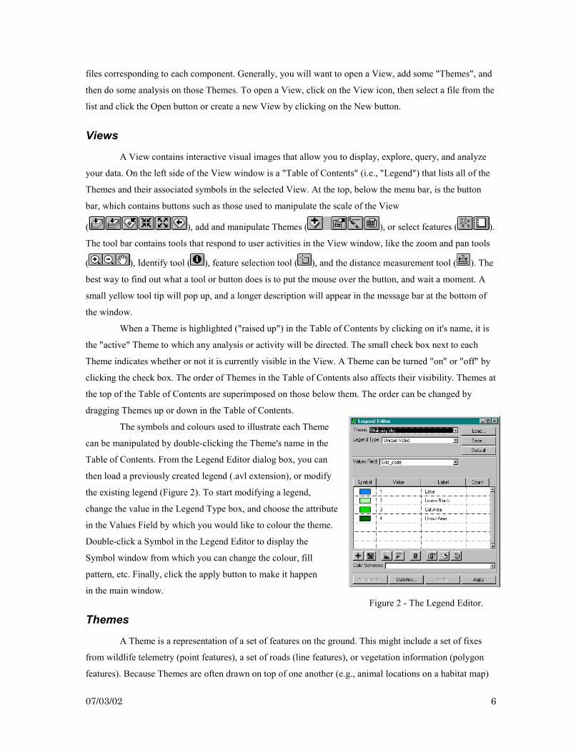
The symbols and colours used to illustrate each Theme

can be manipulated by double-clicking the Theme's name in the

Table of Contents. From the Legend Editor dialog box, you can

then load a previously created legend (.avl extension), or modify

the existing legend (Figure 2). To start modifying a legend,

change the value in the Legend Type box, and choose the attribute

in the Values Field by which you would like to colour the theme.

Double-click a Symbol in the Legend Editor to display the

Symbol window from which you can change the colour, fill

pattern, etc. Finally, click the apply button to make it happen

in the main window.

Themes

A Theme is a representation of a set of features on the ground. This might include a set of fixes

from wildlife telemetry (point features), a set of roads (line features), or vegetation information (polygon

features). Because Themes are often drawn on top of one another (e.g., animal locations on a habitat map)

Figure 2 - The Legend Editor.

07/03/02 7

they are commonly referred to as "layers". To add Themes to a View, click the Add Theme ( ) button, or

click the "Add Theme" item on the View menu. In the dialog that pops up, find the shape file (.shp

extension) or ARC/INFO® coverage you would like to add to your View. Please note that to add LOTEK

.DAT files as Themes, you will first have to use the "Import Fix Data" item from the Home Range menu

(see below).

Tables

Information about the features displayed in a Theme are given in an "Attribute Table". Attributes

are non-spatial data associated with spatial data (e.g., the age, sex and identification number of an animal at

a particular point). To look at the Table for an active Theme, click the Open Theme Table ( ) button.

Once the Theme Table is opened, you can add or edit the information by selecting the "Start Editing" item

from the Table menu. When you are finished making changes, select "Stop Editing" from the Table menu.

Queries

There are two main types of queries available in ArcView. You can click on features using the

Identify tool ( ), or use a database query to select features by some attribute.

The Identify tool ( ) is an easy way to find information about a single feature. Click the tool, then click

on a feature in the active Theme. A box will pop up with

the attributes shown for that feature.

To make a database query, click the Query

Builder ( ) button. A dialog box will pop up (Figure 3).

In the Fields list, double-click the attribute by which you

would like to select features. Click a relationship (>, <>, =,

etc) and then double-click a value in the Values list. If you

then click New Set, the features that match the query will

be selected in the View and any previously selected

features that do not match the query will be deselected. If

you click Add To Set, the matching features will be added to the existing set of selected features. To refine

an existing selection of features, use the Select from Set button.

Temporary Files

When you add a Theme to a Project or generate a new Theme (e.g., by calculating a home range

estimate), ArcView creates several "temporary" files. In fact, these files are not temporary but remain in

your system even after you exit from ArcView. Files with a .shp extension store feature geometry, those

with a .shx extension store an index of the feature geometry, and .dbf files are dBASE files that store

attribute information. These files are stored in the directory indicated by the TEMP environment variable in

Figure 3. Query dialog box.

07/03/02 8

your system, usually c:\temp. If you are uncertain and want to determine the directory in which these files

will be stored, open a DOS prompt window and type SET. In the list of environment variables that are

displayed, you should find a line such as "SET TEMP=c:\temp". If you don't see it, you can add it to your

AUTOEXEC.BAT file using a text editor (Windows 95) or use the System icon in the Control Panel to set

the TEMP variable (Windows NT). Although it is often advantageous to have these files available for

further use, you may eventually encounter problems with the memory capacity of your system and it will

be necessary to remove some of these files.

Viewing and Saving Results

As outlined above, you can use the Identify tool ( ) to quickly browse features in an active

Theme. For example, if you generate a home range polygon using any of the MCP or kernel methods in the

HRE, you can click on the Identify tool ( ) then click on the polygon to see the area of the home range,

number of points used in the estimate, etc. If you want to view the attributes of all the features in the active

Theme, click the Open Theme Table ( ) button. At this point the attributes are already saved in a dBASE

file (see above) and can be used by spreadsheet programs. However, you can also select "Export" from the

File menu and save the attributes in a comma-delimited text file (.txt extension) that can be used in a text

editor or word processor. If you don't want to save the attributes of all the features, you can use the Select

Feature tool ( ) to click on the features you want before opening the Theme Table. Alternatively, once

the Theme Table is open you can click the Select tool ( ) and click the record you want to save. To select

more than 1 record using this method, hold the SHIFT key down while you click on each record you want

from the Theme Table. Yet another way to select a subset of features is to use the Query Builder button

( ) as outlined above. Using any of these methods to choose a subset of features will result in the

selected records being highlighted in the Theme Table. To save only the highlighted records select "Export"

from the File menu, choose the format in which you want to save the data, then specify the name and

location of the file that will be created.

07/03/02 9

Installing the Home Range Extension The HRE requires ArcView 3.0a, running under Windows NT (version 4.0) or Windows 95. To

install the HRE, start ArcView and open the Project named "install.apr" on the distribution diskette, or in

the distribution archive. The install Script will ask you whether this is a network install or a local install. If

it is a local install, the components will go into the main ArcView distribution. If it is a network install, the

components will go to directories to which you have write access.

There is one file that cannot be installed automatically by the network install. It is called

"avdlog.dll", and it is in the file "bin.zip". This .dll file is from the Dialog Designer extension to ArcView.

If the Dialog Designer is installed, then there is no need for concern. If the Dialog Designer has not been

installed and you do not have write access to the destination directory, then you must contact your network

administrator. The install Script will tell you where "avdlog.dll" should be copied. Please note that the

network administrator can do a "local install" and make the extension available to all users. The installation

of the ArcView Dialog Designer is entirely optional.

To uninstall the HRE, you will have to remove the following files from your system;

HOMERANG.AVX, MOOSE.BMP, PAUSE.BMP, PLAYFWD.BMP, REWIND.BMP, KERN.DLL,

DATFILE.DLL. These files will be found in the ESRI\AV_GIS30\ARCVIEW\EXT32 directory. You may

also want to remove any of the temporary files created by using the HRE extension. These files are stored

in the directory indicated by the TEMP environment variable in your system, usually c:\temp (see above).

Adding the Extension to a Project

To use the HRE, open a new Project in ArcView. Once the "Untitled" Project is open, click on the

File menu and choose "Extensions…” In the dialog box that appears, place a check mark in the box beside

Home Range Analysis. If you want the HRE to be loaded each time ArcView is started, click the Make

Default button. The HRE will then be loaded automatically whenever you open a new Project. The

functions in the HRE are available from any View, under the Home Range menu, and on the button and

tool bars.

Saving your Project

When you save your Project using the Save Project button ( ) ArcView saves the current state

of your Project, including your dependence on the HRE. If you want to open your Project on another

machine that does not have the HRE installed, you must remove the extension from the Project (click on

the File menu, choose "Extensions…” and uncheck Home Range Analysis) and save the Project again.

07/03/02 10

Importing Fix Data Fix data comes in a wide variety of formats. You may already have it in ArcView as a Theme, you

may have it in a spreadsheet or database file, or a simple text file. Since the HRE was developed at a site

using LOTEK GPS collars, we have developed an import filter for the data files produced by their

GPSHOST and N3WIN software (.DAT files).

LOTEK .DAT files

LOTEK .DAT files are a binary format containing the location of the fix (latitude, longitude,

time), the quality of the fix (DOP, Convergence), and some ancillary data (temperature, activity sensor).

There are two sub-formats we know of, one for very early collars, and another for more recent collars. This

software supports the newer collar format. If you are using the older format, you will first have to use

LOTEK’s software to export to a text file that can then be imported by the HRE (see below).

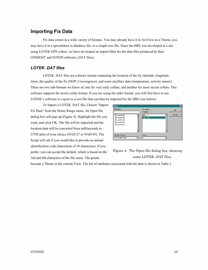
To import a LOTEK .DAT file, Choose "Import

Fix Data" from the Home Range menu. An Open file

dialog box will pop up (Figure 4). Highlight the file you

want, and click OK. The file will be imported and the

location data will be converted from milliseconds to

UTM units of your choice (NAD 27 or NAD 83). The

Script will ask if you would like to provide an animal

identification code (maximum of 10 characters). If you

prefer, you can accept the default, which is based on the

3rd and 4th characters of the file name. The points

become a Theme in the current View. The list of attributes associated with the data is shown in Table 1.

Figure 4. The Open file dialog box, showing

some LOTEK .DAT files.

07/03/02 11

Table 1. Attributes of data imported from a LOTEK .DAT file.

Attribute Description

Lon longitude in milliseconds (West is negative)

Lat latitude in milliseconds (North is positive)

Time seconds since midnight, 1/1/1970

Dop dilution of precision

Fix fix status (2D, 3D, Differential)

Temp temperature (°C)

Act average activity count in time interval between fixes

Con convergence

Easting Easting in UTM co-ordinates

Northing Northing in UTM co-ordinates

Zone UTM zone

Date date coded as YYYYMMDD in a number

TimeOfDay time coded as HHMMSS in a number

Animal animal identification code

Argos DCLS Files

The HRE also provides direct import of data from Service Argos Data Collection and Location

System (DCLS) files. To import one of these files, choose "Import Fix Data" from the Home Range menu.

An Open file dialog box will pop up. In the List Files Of Type box, select "Tab-delimited Text Files" as the

file type. Highlight the file you want, and click OK. You will be asked to confirm that the selected file is an

Argos file. Next, you will be asked to choose an X co-ordinate. Highlight Mslon in the dialog box and click

OK. You will also be asked to choose a Y co-ordinate. Highlight Mslat and click OK. Since Mslat and

Mslon are in milliseconds, the Script will ask if the points should be converted to UTM units from

thousands of seconds. You should answer "Yes", then indicate the UTM units you would like to use (NAD

27 or NAD 83). This will create 2 new fields called "xcoord" and "ycoord" which contain the Easting and

Northing, respectively, in the selected UTM co-ordinate system. Since there is a column called "Time" in

the import file, the Script will ask if the time should be converted from seconds since midnight, 1/1/1970.

Although the import filter does this conversion automatically and places the results in the Time field, you

should answer "Yes". This will add 2 fields called "Date" and "TimeOfDay" which are used to sequence

data in several HRE procedures. To finish importing the file, you will be asked if you would like to provide

an animal identification code (maximum of 10 characters). If you answer "Yes" and enter a code or click

OK to accept the default, a field called "Animal" will be added to the Theme Table and the code will be

07/03/02 12

used in the Theme name. If you answer "No", the Theme name will be based on the original file name and

no animal identification field will be added to the Theme Table. At the end of the import process, the points

become a Theme in the current View. The list of attributes associated with the data is shown in Table 2.

Table 2. Attributes of data imported from an Argos DCLS .txt file.

Attribute Description

Mslat latitude in milliseconds (North is positive)

Mslon longitude in milliseconds (West is negative)

Program Service Argos program #

Platform platform (PPT) identification # (i.e., collar #)

Satellite code for the satellite receiving the data

Class Argos location quality index

Date date coded as YYYYMMDD in a number

Daytime time coded as HHMMSS in a number

Time seconds since midnight, 1/1/1970

Latitude Northing in decimal degrees

Longitude Easting in decimal degrees

Frequency calculated UHF frequency of the transmission

xcoord Easting in UTM co-ordinates

ycoord Northing in UTM co-ordinates

Date date coded as YYYYMMDD in a number

TimeOfDay time coded as HHMMSS in a number

Animal animal identification code (optional)

Text Files and dBASE Files

Text files (comma-separated values, tab-delimited ASCII) or dBASE files are treated identically.

To import one of these files, choose "Import Fix Data" from the Home Range menu. An Open file dialog

box will pop up. In the List Files Of Type box, select the file type you are looking for. Highlight the file

you want, and click OK. The file will be imported with a few questions (see below). The points become a

Theme in the current View.

Imported location data must be in UTM units (NAD 83 or NAD 27) or milliseconds of latitude

and longitude. If your location data are in UTM units, they should be in columns or fields called "northing"

(first column) and "easting" (second column). Similarly, if your data are in milliseconds, they should be in

columns or fields called "lat" and "lon". In this case, the Script will ask if the points should be converted to

UTM units from milliseconds of latitude and longitude. You should answer "Yes". If your data are recorded

07/03/02 13

in some other format (answer "No"), such as decimal degrees, you can import them in the usual ArcView

way (ESRI 1996) but some of the HRE options may not work correctly.

The HRE uses a "time" field to sequence data in several of its procedures. Thus, locations in your

imported file should be associated with a linear "time" scale that provides a unique value for each point,

otherwise some of the HRE options will not work correctly. Although seconds since 1/1/1970 is the

preferred HRE format, any linear scale can be used. In fact, you could simply order your data and number

the sequence from first to last in a column called "time". If there is a column called "time" in the import

file, the Script will ask if these data should be converted from seconds since midnight, 1/1/1970. Select

"Yes" only if your time data are recorded as seconds since midnight, 1/1/1970. This will add two fields;

"Date" and "TimeOfDay" (Tables 1 and 2). If you have used a different linear "time" scale (select "No"),

these new fields will not be created but the HRE will still function correctly.

Lastly, the Script will ask if you would like to add an animal identification code (maximum of 10

characters).

ARC/INFO Coverages

ARC/INFO coverages can be added to the View as a Theme in the normal ArcView way using the

Add Theme ( ) button. Find the coverage and highlight it in the Add Theme dialog box, then click the

OK button.

Other Information

All sorts of other information can be imported into ArcView, in a variety of ways. A good

reference for bringing information into ArcView is "Using ArcView GIS", from ESRI (1996). The help file

supplied with ArcView is also a useful resource.

07/03/02 14

Editing Fix Data Sometimes there are irrelevant fixes that need to be removed from data files before further

analyses can proceed. For instance, locations recorded by Lotek GPS collars during the initialization

process, prior to deployment on animals. Another problem is the occurrence of duplicate points in a data

file. This might occur if a downloading session with a Lotek GPS collar is interrupted. Upon resumption of

the download, if the user chooses to append data to a previously created file rather than overwriting it,

duplicate records may be stored. Duplicate records might also occur when files are merged (see below).

Argos DCLS, text, and dBASE files should be converted to "shapefiles" before editing (select "Convert to

Shapefile" from the Theme menu).

Removing individual points

With the Theme to be edited active in the View, choose "Start Editing" from the Theme menu.

Select the point to be removed in the View using the Select Feature tool ( ) or use the "Query" function

on the Theme menu. Press the Delete key on the keyboard. When you are finished removing points, select

"Stop Editing" from the Theme menu.

Removing Duplicates

Rather than manually editing a Theme Table, there is an easy way to remove duplicates in a

Theme using the HRE. Make the Theme you would like to check active. Select "Merge Coverages" from

the Home Range menu. If there are any duplicates in the file, a dialog box will pop up and ask which record

to drop. A new Theme will be created with the duplicate removed. This procedure is identical to the

procedure for merging Themes (see below), with the exception that only one input Theme is involved.

Merging Themes

To merge Themes, such as multiple downloads from the same animal’s collar, make the Themes

you would like to merge active. To make more than one Theme active, hold the Shift key down as you

click a second Theme in the Table of Contents. Choose "Merge Coverages" from the Home Range menu. A

new Theme will be created containing all the features from the input Themes. The attribute types of all

Themes involved should be identical before they are merged. After the Themes are merged, a check is

performed for duplicates based on the "time" field. If there are any duplicates, a box will pop up to ask the

user which point to drop. The new Theme will be sorted by the "time" field, if available.

07/03/02 15

Exploratory There are two major exploratory data analysis tools available in the HRE; basic ArcView queries,

and “Moose On A Leash” (MOAL). The queries use the Identify tool ( ) and the Table associated with a

Theme, as previously described. MOAL, on the other hand, is an interactive data walkabout tool.

“Moose On A Leash”

The "Moose On A Leash" (MOAL) option lets you follow an animal's path as it moves from point

to point in the View window. To explore all of the movements in a data set, select the Theme that you

would like to use and make it active. Only one Theme at a time can be processed. If you don't want to use

the entire Theme, you can use the Select Feature tool ( ) to drag a box around a subset of the points in

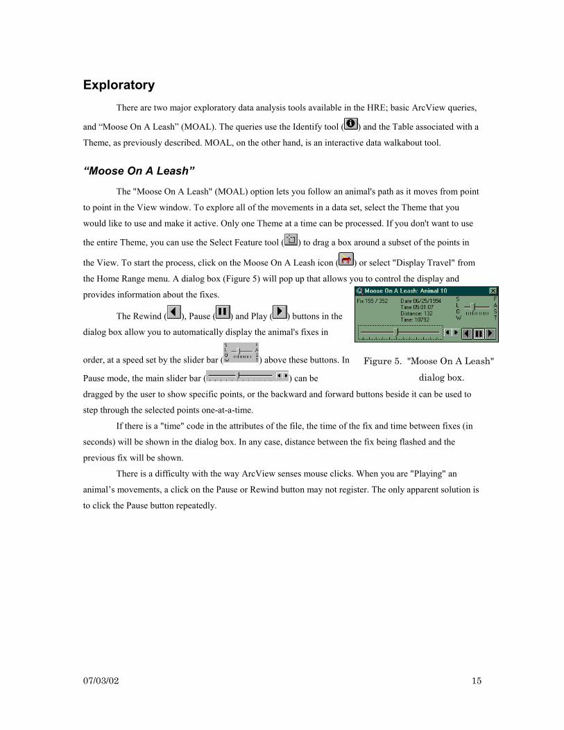
the View. To start the process, click on the Moose On A Leash icon ( ) or select "Display Travel" from

the Home Range menu. A dialog box (Figure 5) will pop up that allows you to control the display and

provides information about the fixes.

The Rewind ( ), Pause ( ) and Play ( ) buttons in the

dialog box allow you to automatically display the animal's fixes in

order, at a speed set by the slider bar ( ) above these buttons. In

Pause mode, the main slider bar ( ) can be

dragged by the user to show specific points, or the backward and forward buttons beside it can be used to

step through the selected points one-at-a-time.

If there is a "time" code in the attributes of the file, the time of the fix and time between fixes (in

seconds) will be shown in the dialog box. In any case, distance between the fix being flashed and the

previous fix will be shown.

There is a difficulty with the way ArcView senses mouse clicks. When you are "Playing" an

animal’s movements, a click on the Pause or Rewind button may not register. The only apparent solution is

to click the Pause button repeatedly.

Figure 5. "Moose On A Leash"

dialog box.

07/03/02 16

Analyzing Fix Data Generating interfix distances and elapsed times or home range polygons from animal locations is a

simple procedure. Select the Theme you would like to analyze, then open the Theme Table ( ) or choose

the analysis you would like to use from the Home Range menu. The analysis will use the points selected in

the Theme(s), unless there are no points selected, in which case the analysis will use all points in the

Theme(s).

Calculating Interfix Times and Distances

Although the MOAL option allows you to step through selected points one-at-a-time and

determine the distance moved and elapsed time between consecutive fixes, you may want to calculate and

save multiple interfix distances and elapsed times, as well as cumulative values for these variables. With

these data you can calculate average distance moved between fixes, average elapsed time between fixes,

speed of movement, total distance moved in a given period, and so on.

Select the Theme that you would like to use and make it active. Click the Open Theme Table

( ) button then choose "Start Editing" from the Table menu. You can now select "Calculate Interfix

Distances" from the Field menu. This will add 2 new columns to the Table, "InterFixD" and "CumD",

which are the distances between consecutive fixes in the file and cumulative distances among the points.

Similarly, if you choose "Calculate Interfix Time" from the Field menu, 2 columns will be added,

"InterFixT" and "CumT", which are the elapsed time between consecutive fixes and cumulative time over

which the points were recorded. After completing your calculations, select "Stop Editing" from the Table

menu and save your results. At this point you can generate some simple summary statistics by clicking on a

field name in the Table (e.g., "InterFixT"), then choose "Statistics" from the Field menu.

If you want to calculate interfix distances and times on a subset of the data or between non-

consecutive fixes, you will have to create a new Theme. Use the Select Feature tool ( ) to drag a box

around the points you want to include. Alternatively, you can use the Query Builder ( ) to select a subset

of points from the active Theme. You could also select points by opening the Theme Table ( ), then

choose the points to be used with the Select tool ( ). After selecting all the points you want to include,

choose "Convert to Shapefile…" from the Theme menu. Specify the name and location of the new Theme

in the dialog box. When prompted to add this new shapefile to your View as a Theme, click Yes. You can

now make the new Theme active and proceed as above.

07/03/02 17

Generating Minimum Convex Polygons

The minimum convex polygon (MCP) Script will make a polygon using the outermost points of a

group of fixes. This Script will process multiple Themes, one at a time, to produce a single Theme

containing polygons. With large numbers of points, it may be slow.

To generate a MCP using all the points in the selected Theme(s), choose "MCP 100%" from the

Home Range menu. To generate a MCP on a subset of the points in the View, use the Select Feature tool

( ) to drag a box around the points, then choose "MCP 100%" from the Home Range menu. To generate

a % MCP using all the points in the selected Theme(s) or a manually selected subset, choose "Percentage

MCP" from the Home Range menu.

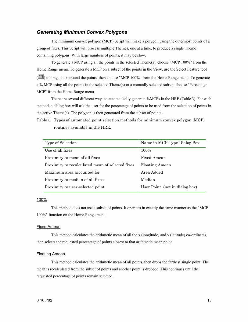
There are several different ways to automatically generate %MCPs in the HRE (Table 3). For each

method, a dialog box will ask the user for the percentage of points to be used from the selection of points in

the active Theme(s). The polygon is then generated from the subset of points.

Table 3. Types of automated point selection methods for minimum convex polygon (MCP)

routines available in the HRE.

Type of Selection Name in MCP Type Dialog Box

Use of all fixes 100%

Proximity to mean of all fixes Fixed Amean

Proximity to recalculated mean of selected fixes Floating Amean

Maximum area accounted for Area Added

Proximity to median of all fixes Median

Proximity to user-selected point User Point (not in dialog box)

100%

This method does not use a subset of points. It operates in exactly the same manner as the "MCP

100%" function on the Home Range menu.

Fixed Amean

This method calculates the arithmetic mean of all the x (longitude) and y (latitude) co-ordinates,

then selects the requested percentage of points closest to that arithmetic mean point.

Floating Amean

This method calculates the arithmetic mean of all points, then drops the farthest single point. The

mean is recalculated from the subset of points and another point is dropped. This continues until the

requested percentage of points remain selected.

07/03/02 18

Area Added

This method drops points based on the amount of area they add to the home range polygon (White

and Garrott 1990). To begin, a 100% MCP is calculated. The points that form the polygon are then deleted

one at a time. After a point is removed a new MCP is constructed and its area is calculated. The difference

in area between the new MCP and the 100% MCP is determined. The point is then restored and the next

point is deleted. After all boundary points are tested, the polygon that had the greatest difference in area

from the 100% MCP is identified and the associated point is dropped. The polygon constructed without this

point becomes the new polygon against which to test the remaining points. This process continues until the

requested percentage of points remain selected. This procedure can be excruciatingly slow, especially with

many points.

Median

This method calculates the median of all the x (longitude) and y (latitude) co-ordinates, then

selects the requested percentage of points closest to that median point.

User Point

To generate a %MCP using a percentage of points closest to a specific location, click the MCP

User tool ( ), then click on the View to define the point. A dialog box will pop up to ask for a percentage

of points to be used in the calculation. A MCP will be built using the requested percentage of points closest

to where you clicked.

Generating Kernel Polygons

The kernel analysis Script produces a set of polygons derived from the calculation of the standard

bivariate normal (i.e., Gaussian) kernel density estimator (i.e., utilization distribution). Polygons may be

calculated from either the kernel densities or volumes of the curve under different portions of the utilization

distribution. A smoothing parameter is calculated automatically and the Script provides both fixed and

adaptive methods of smoothing the kernel density estimator.

07/03/02 19

To start a kernel analysis, select the Theme containing the fixes for which you would like to

generate polygons. Only one Theme at a time can be processed. To produce polygons from a subset of the

points in the View, use the Select Feature tool ( ) to drag a box around the points. Choose "Kernel

Analysis" from the Home Range menu. A dialog box will pop up that provides indices that can be used to

assess the independence of your observations and allows you

to select parameters for fixed or adaptive kernel analysis

(Figure 6). You can change the smoothing parameter, type of

smoothing, resolution, contouring type, and contour levels (if

using volume contours).

Independence of Observations

Independence of successive animal locations is a

basic assumption of many statistical methods of home range

analysis. Temporal autocorrelation (sometimes called "serial

correlation") of fix data tends to underestimate true home

range size in these models (Swihart and Slade 1985a).

Schoener (1981) proposed a statistic for detecting departures

from independence of observations based on the ratio of the

mean squared distance between successive observations and

the mean squared distance from the centre of activity. Significant deviations of Schoener's index from an

expected value of 2.0 (i.e., <1.6 or >2.4) indicate a strong correlation between distance and time (i.e., the

animal did not have time to move very far before it was located again or it is repeating a previous pattern of

movements). Swihart and Slade (1985a) derived the sampling distribution of Schoener's index and provided

a test of independence that can be used to determine the time to independence between observations (i.e.,

the minimum time interval between successive observations that allows them to be considered

independent). They later provided their own bivariate measure of autocorrelation, which included terms for

both serial correlation and cross correlations (Swihart and Slade 1985b). High values of the Swihart and

Slade index (i.e., >0.6) indicate significant autocorrelation (Ackerman et al. 1990). Both Schoener's (1981)

index and the Swihart and Slade (1985b) index are given at the top of the kernel analysis dialog box (Figure

6). If your data are autocorrelated you might consider randomly deleting locations until these indices are no

longer significant (Ackerman et al. 1990) or, more objectively, use the method developed by Swihart and

Slade (1985a) to determine the time to independence and remove the intervening locations.

Choice of Smoothing Parameter

Choosing an appropriate smoothing parameter (i.e., "bandwidth") is the most important step in

deriving a kernel density estimator (Worton 1989) but there is no agreement on how to approach this

problem (Silverman 1986). The smoothing parameter (h) determines the spread of the kernel that is centred

Figure 6. Kernel Procedure

Parameters dialog box.

07/03/02 20

over each observation. If the value of h is small, individual kernels will be narrow and the kernel density

estimate at a given point will be based on only a few observations. This may not allow for variation among

samples and may produce an extremely variable (i.e., "undersmoothed") utilization distribution. On the

other hand, if the value of h is large, individual kernels will be wide and the resulting "oversmoothed"

utilization distribution may obscure the fine detail required to identify centres of activity. The HRE

provides several automated and subjective methods of finding the "best" value of h for a given situation.

Since h is an expression of the variances of the x (varx) and y (vary) co-ordinates around a given

point, and these may be unequal if they are estimated from the observations, it is advisable to rescale the

data before any kernel method is applied (Worton 1989). The HRE provides 2 methods of standardizing

data (Figure 6) that should produce the same results. Both are included because they have been used by

different authors, but there are no studies available to suggest which of these methods might be preferred in

different situations. "Unit Variance" changes the co-ordinates of the fixes by dividing each value of x and y

by its respective standard deviation (Seaman and Powell 1996). The "X Variance" setting transforms the y

co-ordinates to have the same variance as the x co-ordinates by dividing each y value by the y standard

deviation and multiplying the result by the x standard deviation (Kenward and Hodder 1996). Although it is

not recommended, you may click "None" for no standardization.

An automated method of choosing a starting value for h is to use the optimum value with

reference to a known standard distribution (i.e., href) (Silverman 1986; Worton 1989, 1995). Since the

HRE uses a standard bivariate normal probability density function to estimate the utilization distribution,

href is calculated as the square root of the mean variance in x (varx) and y (vary) co-ordinates divided by

the sixth root of the number of points (Worton 1995);

2var

nh yx61

ref

var+= −

The value of href for the points selected in the View window is given in the kernel analysis dialog box

(Figure 6).

The href method is effective if the underlying utilization distribution is unimodal (i.e., "single-

peaked") (Worton 1995). This may be sufficient to describe a concentrated group of points selected in a

View window, but will usually oversmooth the utilization distribution for an entire Theme because animals

typically have multiple centres of activity within their home range.

Least-squares cross-validation (LSCV) is a common method for automatically calculating the

smoothing parameter (select "h_cv" in the kernel analysis dialog box). The LSCV method attempts to find

a value for h that minimizes the mean integrated square error (MISE) by minimizing a score function

CV(h) for the estimated error between the true density function and the kernel density estimate (Worton

1995);

22

2D

4D

n

1j

n

1i2 hn

e1e41

nh1hCV

ijij

−+=

−−

==∑∑

πππ

)(

07/03/02 21

where the distance between pairs of points (Dij) is calculated as;

2

2yjyi

2xjxi

2ji

ij hXXXX

hXX

D)()()( )()()()( −+−

=

−=

The minimum value of CV(h) is found by testing values of h between 0.01href and href, selected using a

"Golden Section Search" algorithm (Press et al. 1986). The resulting smoothing parameter that minimizes

the score function is called hcv.

In situations where the utilization distribution is not unimodal, the LSCV method has been shown

to overcome the problem of oversmoothing associated with the use of href (Worton 1989). However, the

LSCV method is not always successful in finding a smoothing parameter that will minimize the MISE. In

these cases, the HRE will report a low value for hcv that is near the smallest value that can be tested (i.e.,

0.01href). This will result in a utilization distribution that is seriously undersmoothed. Indeed, the LSCV

method has a propensity to show structure in the data when none exists (Sain et al. 1994).

A technique that may strike a balance between the tendency of href to oversmooth and hcv to

undersmooth utilization distributions is biased cross-validation (BCV) which is implemented by selecting

"h_bcv2" in the kernel analysis dialog box (Figure 6). In contrast with the LSCV method, BCV attempts to

find a value for h that minimizes an estimate of the asymptotic mean integrated square error (AMISE).

AMISE is a large sample (e.g., n>50) approximation of the MISE (Wand and Jones 1995). Thus, it also

provides an estimate of the difference between the true density function and the kernel density estimate.

However, it is computationally faster and easier to calculate than MISE and provides a more direct

indication of the performance of h values (Sain et al. 1994, Wand and Jones 1995, Jones et al. 1996). In the

HRE, the function to be minimized is (Sain et al. 1994);

ππ 2

2D

ij2ij

n

1j

n

1i2 h2n1n8

e8D8D1nh4

1h2BCV

2ij

))(()(

)()(

−−+−

+−

=

−

==∑∑

where the distance between pairs of points (Dij) is again calculated as;

2

2yjyi

2xjxi

2ji

ij hXXXX

hXX

D)()()( )()()()( −+−

=

−=

Similar to the LSCV method, values of h between 0.01href and href, are selected for testing using a "Golden

Section Search" algorithm (Press et al. 1986). The resulting smoothing parameter is called hbcv2.

Simulation studies show the BCV method performs quite well and with reasonable variability in

comparisons with the LSCV and reference methods (Sain et al. 1994). However, the BCV method has not

been investigated in the context of home range estimation.

In the event that the automated methods do not provide a suitable value for the smoothing

parameter, the HRE allows you to input a subjective choice (select "h_user" in the kernel analysis dialog

box). This feature is particularly useful for data exploration and hypothesis generation. You can enter a

"raw" smoothing parameter directly by clicking on the "h" field and editing the default value (1.00000),

07/03/02 22

provided the "h/href" checkbox is not selected. Alternatively, you can test a proportion or multiple of href

by selecting the "h/href" checkbox and editing the default multiplier (1.00000) in the "h" field. In addition

to helping you choose the "best" smoothing parameter, these subjective methods allow you to highlight

various features of a home range dataset that may not be immediately obvious from a simple plot of animal

locations.

Fixed/Adaptive Smoothing

The HRE allows the user to select either "Fixed" or "Adaptive" kernel methods of estimating the

utilization distribution. The fixed kernel approach assumes the width of the standard bivariate normal

kernel placed at each observation is the same throughout the plane of the utilization distribution. This can

be problematic if there are outlying regions of low density because it is difficult to select a smoothing

parameter that will accommodate these outer areas without oversmoothing the core of the distribution. The

adaptive kernel method, on the other hand, allows the width of the kernel to vary such that regions with low

densities of observations have higher h values and are smoothed more than areas of high concentration.

Before an adaptive kernel estimate can be calculated, a "pilot" estimate of the utilization distribution must

be obtained. This initial estimate is used to determine the pattern of kernel widths across all observations

and ultimately the adaptive estimator itself (Silverman 1986). The smoothing parameter selected in the

kernel analysis dialog box (Figure 6) will be used by the HRE to obtain both the pilot estimate and the

adaptive kernel estimate of the utilization distribution.

Whereas Worton (1989) found adaptive kernel estimates using the LSCV choice of h provided

better results than the fixed kernel method, Seaman and Powell (1996) found the opposite. One explanation

is that the widening of kernels in outlying regions by the adaptive approach may produce unacceptable

expansion of the utilization distribution (Kenward and Hodder 1996). It is more likely, however, that these

differences in performance of the 2 methods are simply a consequence of the different sets of observations

used in each study. Therefore, we suggest the choice of which smoothing approach to use depends on the

original observations and is left up to the user to determine through exploration of their data.

Volume/Density Contouring

Two types of contouring are supported in the HRE (Figure 6); density (D) contouring and volume

(V) contouring. Density contours surround regions of constant probability density. Selecting this option

will produce 8 contour lines (i.e., isopleths) in the View window. Moving inward from the outermost

contour line, which surrounds 1/8 x the maximal probability density function value, each successive

isopleth surrounds an additional 1/8 x the maximal probability density function value. Thus, the innermost

contour line encompasses 7/8 x the maximal probability density function value. Volume contours, on the

other hand, are determined from volumes under the utilization distribution and connect regions of equal

probability. Thus, for example, the 95% volume contour surrounds an area within which an animal spends

95% of its time (i.e., there is a 95% chance of finding the animal within that area). A particular volume

07/03/02 23

contour may or may not include the same proportion of observations due to smoothing of the kernel

function and round off errors (e.g., the 95% volume contour may not contain 95% of the locations).

Although the two methods will produce similar contours, volume contours are generally used in home

range analysis. If you use volume contours, you can enter specific probabilities separated by commas in

the "levels" box, or you can leave the field blank and the HRE will draw 9 contours, spaced by 0.1

probability levels.

Choice of Resolution

The kernel methods implemented in the HRE calculate probability density estimates at the centre

of each cell in a raster (i.e., grid) of cells. The process is theoretically independent of resolution. However,

preliminary tests indicate that resolutions below 50x50 grid cells may produce home range estimates that

are not consistent with area calculations based on higher resolutions. This may be caused by the inherent

angularity of contours derived from a low-resolution raster. On the other hand, although there is no

theoretical upper limit to the resolution that could be used, memory concerns between ArcView and the

operating system limit the practical resolution to about 150x150. Analyses at higher resolutions will be

calculated more slowly, and may cause ArcView to "hang" (above a resolution of about 150). This problem

is hard to predict and has not been completely investigated. If you choose to use a resolution above

120x120, make sure you save your Project before running the kernel procedure. The default resolution is

70, which is a compromise between the limited accuracy of low resolutions and speed.

07/03/02 24

Analyzing Habitat Use Determination of habitat types used by an animal is relatively straightforward in a GIS using an

overlay function. The "habitat used by the animal" is the geometric intersection of "the habitat" with "the

area used by the animal" as described by a polygon resulting from one of the MCP or kernel methods. A

habitat map can be produced from satellite imagery, forest resource inventory maps, aerial photography,

etc. The production of the habitat map is not within the scope of the HRE, although ArcView may be

involved in the classification or presentation of the data. The HRE supports habitat maps created with a

UTM coordinate system using the NAD 83 or NAD 27 spheroid.

To determine proportions of habitat types within a home range, select the Theme that you would

like to use. Only one home range Theme at a time can be processed. If you don't want to use the entire

Theme, you can use the Select Feature tool ( ) to select a subset of the polygons in the View. Note that if

you use the selection tool ( ) to choose a subset of contours from a home range calculated by one of the

kernel methods, the contour you click on and all those at a higher level will be selected (e.g., if you click

inside the 70% contour, the 70, 80 and 90% contours will be selected). If you want to use specific contours,

these can be selected with the Query Builder button ( ) or the "Query" item on the Theme menu. Ensure

that both the home range Theme and the habitat Theme are active, then choose "Clip Theme" from the

Home Range menu. A dialog will pop up to ask you to identify the clipping Theme. Generally, this will be

the home range Theme. The shape used to clip the habitat will be derived from a union of all the shapes

selected in the clipping Theme. A new Theme will be produced containing the polygons from the habitat

map that are inside the home range polygons.

Analysis of the clipped Theme is performed in the same way as you would query any other

Theme. The Identify tool ( ) and the "Query" item on the Theme menu will be useful, as will viewing

the Theme Table ( ).

Overlap Analysis

Determination of areas of overlap between home ranges is achieved by the same methods used for

analyzing habitat within home range polygons. First, select the Themes that you would like to use. As

before, if you don't want to use an entire Theme, you can use the Select Feature tool ( ) or Query Builder

button ( ) to select a subset of the polygons within each Theme. Ensure both home range Themes are

active, then choose "Clip Theme" from the Home Range menu. A dialog will pop up to ask you to identify

the clipping Theme. Either home range Theme can be used. A new Theme will be produced containing the

area of overlap. Once again, the Identify tool ( ), the "Query" item on the Theme menu, and the Open

Theme Table ( ) button can be used to view the results.

07/03/02 25

Combining Themes

When Themes are merged using the methods previously described, the features of the original

Themes are maintained in the new Theme that is created. For example, if two polygons overlap, the

boundaries of the overlap are maintained and the attributes of both polygons will be given in the Theme

Table ( ). This may be useful in some situations, but there may be circumstances where you want to

create a new Theme that combines the features of the original Themes. This is a 2-step process: the Themes

are merged, then a "union" of selected features is created.

Begin by selecting the Themes that you would like to use. Once again, if you don't want to use an

entire Theme, you can use the Select Feature tool ( ) or Query Builder button ( ) to select a subset of

the polygons within each Theme. Ensure both home range Themes are active, then choose "Merge

Coverages" from the Home Range menu. As before, this creates a new Theme containing all the features

from the input Themes. Make this newly created Theme active, then use the Select Feature tool ( ) or

Query Builder button ( ) to select the polygons you want to combine. You can also select polygons by

opening the newly created Theme Table ( ), then use the Select tool ( ) to choose the polygons to be

combined (remember, when using this selection method to select more than 1 record, hold the SHIFT key

down while you click on each record you want from the Theme Table). Click the Union Selection button

( ) or choose "Union Selection" from the Home Range menu and another new Theme will be created

that combines the features selected from the merged Themes. As always, the Identify tool ( ), the Open

Theme Table ( ) button, and the "Query" item on the Theme menu can be used to view the results.

07/03/02 26

References Ackerman, B. B., F. A. Leban, M. D. Samuel, and E. O. Garton. 1990. User's manual for program HOME

RANGE. Second ed. For., Wildl. and Range Exp. Stn., Univ. Idaho, Moscow, ID. Tech. Rep. 15.

80 pp.

Burt, W. H. 1943. Territoriality and home range concepts as applied to mammals. J. Mammal. 24:346-352.

(ESRI) Environmental Systems Research Institute. 1996. Using ArcView GIS. Environmental Systems

Research Institute, Inc., Redlands, CA. 350 pp.

Harris, S., W. J. Cresswell, P. G. Forde, W. J. Trewhella, T. Woollard, and S. Wray 1990. Home-range

analysis using radio-tracking data - a review of problems and techniques particularly as applied to

the study of mammals. Mammal Rev. 20:97-123.

Jones, M. C., J. S. Marron, and S. J. Sheather. 1996. A brief survey of bandwidth selection for density

estimation. J. Amer. Stat. Assoc. 91:401-407.

Kenward, R. 1987. Wildlife radio tagging. Academic Press, Inc., London, UK. 222 pp.

Kenward, R. E., and K. H. Hodder. 1996. RANGES V: an analysis system for biological location data. Inst.

Terrestrial Ecol., Furzebrook Res. Stn., Wareham, UK. 66 pp.

Larkin, R. P., and D. Halkin. 1994. A review of software packages for estimating animal home ranges.

Wildl. Soc. Bull. 22:274-287.

Lawson, E. J. G., and A. R. Rodgers. 1997. Differences in home-range size computed in commonly used

software programs. Wildl. Soc. Bull. 25:721-729.

Michener, G. R. 1979. Spatial relationships and social organization of adult Richardson's ground squirrels.

Can. J. Zool. 57:125-139.

Mohr, C. O. 1947. Table of equivalent populations of North American small mammals. Am. Midl. Nat.

37:223-249.

Press, W. H., B. P. Flannery, S. A. Teukolsky, and W. T. Vetterling. 1986. Numerical recipes: the art of

scientific computing. Cambridge Univ. Press, Cambridge, UK. 818 pp.

Rodgers, A. R., R. S. Rempel, and K. F. Abraham. 1996. A GPS-based telemetry system. Wildl. Soc. Bull.

24:559-566.

Sain, S. R., K. A Baggerly, and D. W. Scott. 1994. Cross-validation of multivariate densities. J. Amer. Stat.

Assoc. 89:807-817.

07/03/02 27

Schoener, T. W. 1981. An empirically based estimate of home range. Theor. Pop. Biol. 20:281-325.

Seaman, D. E., and R. A. Powell. 1996. An evaluation of the accuracy of kernel density estimators for

home range analysis. Ecology 77:2075-2085.

Silverman, B. W. 1986. Density estimation for statistics and data analysis. Chapman and Hall, Ltd.,

London, UK. 175 pp.

Swihart, R. K., and N. A. Slade. 1985a. Testing for independence of observations in animal movements.

Ecology 66:1176-1184.

Swihart, R. K., and N. A. Slade. 1985b. Influence of sampling interval on estimates of home-range size. J.

Wildl. Manage. 49:1019-1025.

Tufto, J. 1994. KERNEL PROGRAM for DOS. Available from: Tom's Wildlife Telemetry Clearinghouse

via the INTERNET (http://www.uni-sb.de/philfak/fb6/fr66/tpw/ telem/dataproc.htm#hr). Accessed

1998 Jan 23.

Wand, M. P., and M. C. Jones. 1995. Kernel smoothing. Chapman and Hall, Ltd., London, UK. 212 pp.

White, G. C., and R. A. Garrott. 1990. Analysis of wildlife radio-tracking data. Academic Press, Inc., San

Diego, CA. 383 pp.

Worton, B. J. 1989. Kernel methods for estimating the utilization distribution in home-range studies.

Ecology 70:164-168.

Worton, B. J. 1995. Using Monte Carlo simulation to evaluate kernel-based home range estimators. J.

Wildl. Manage. 59:794-800.