Embed Size (px)
Citation preview
H.P. WILLIAMS
LONDON SCHOOL OF
ECONOMICS
MODELS FOR SOLVING
THE
TRAVELLING SALESMAN PROBLEM
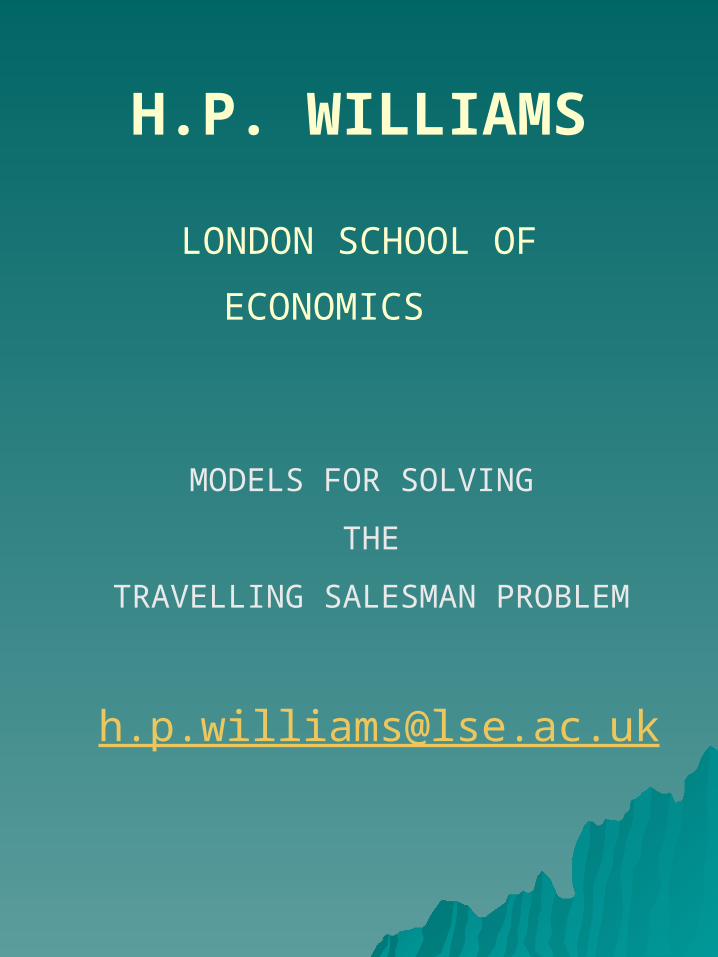
STANDARD FORMULATION OF THE (ASYMMETRIC) TRAVELLING
SALESMAN PROBLEM
Conventional Formulation:
(cities 1,2, …, n) (Dantzig, Fulkerson, Johnson) (1954). is a link in tour
Minimise:
subject to:
ji
ijijxc
,
}...,{,
nSSxijSji
2 all 1 - | |
1 all ijj
x i
1 all iji
x j
ijx
62
3
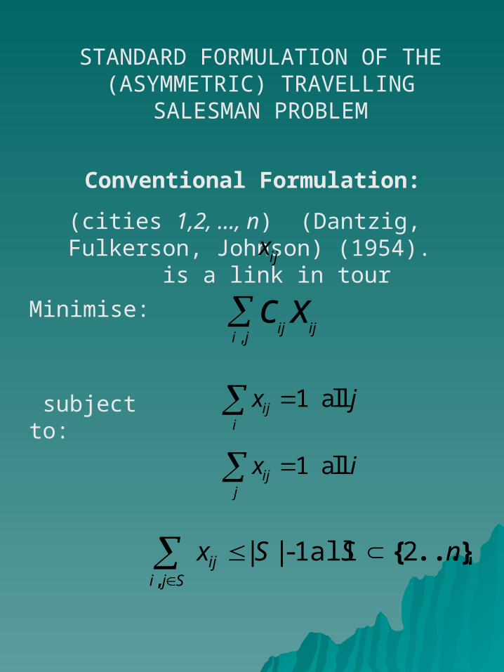
e.g.
632632 xxx
2366223 xxx
0(2n) Constraints = (2n-1 + n –2) 0(n2) Variables = n(n – 1)
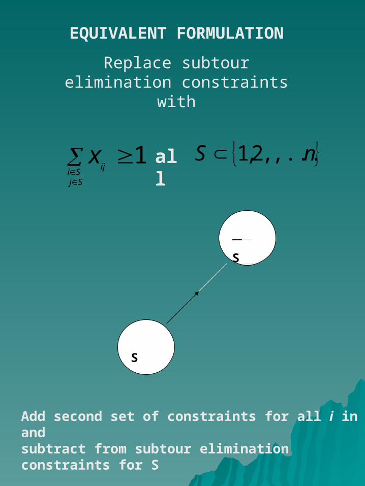
EQUIVALENT FORMULATION
Replace subtour elimination constraints with
1
SjSi
ijx all nS ,...,,2,1
____
S
S
Add second set of constraints for all i in S and subtract from subtour elimination constraints for S
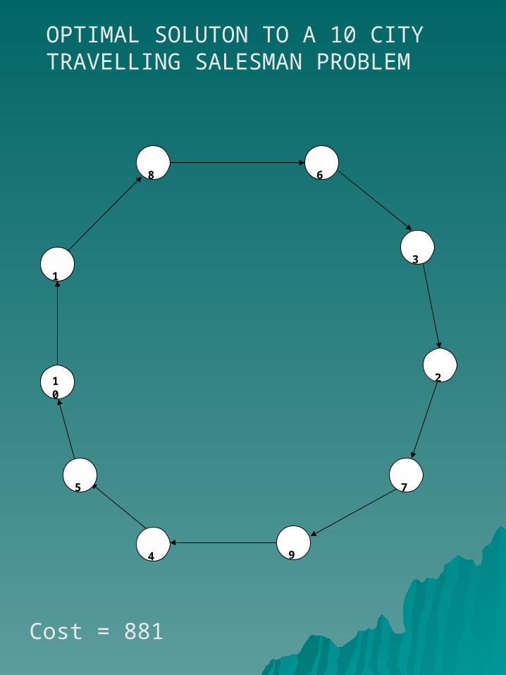
OPTIMAL SOLUTON TO A 10 CITY TRAVELLING SALESMAN PROBLEM
10
1
8 6
3
2
7
9
5
4
Cost = 881
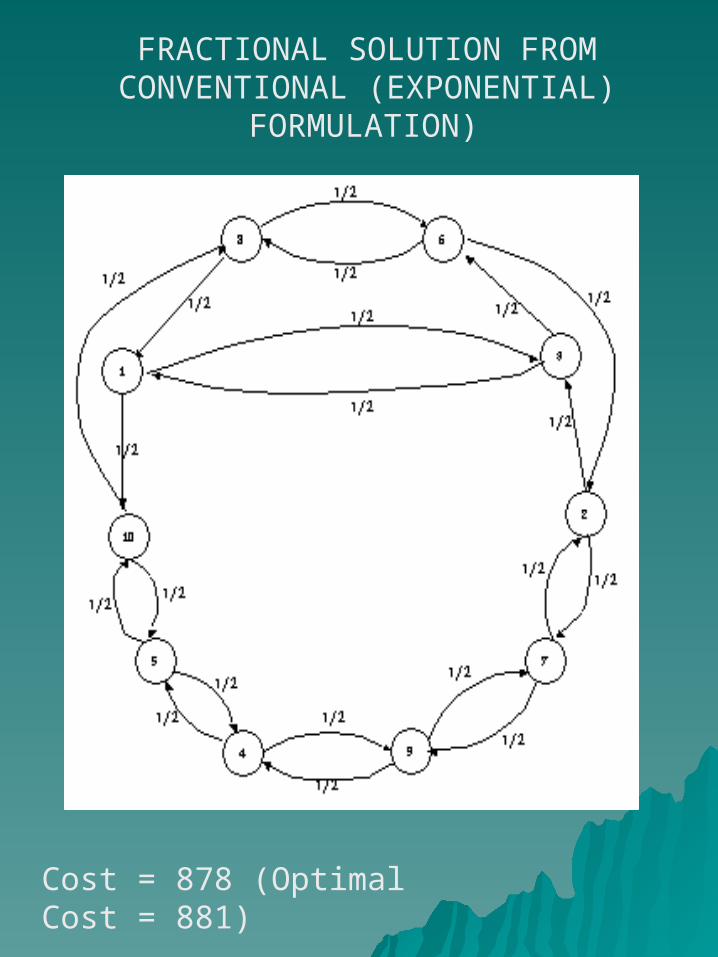
FRACTIONAL SOLUTION FROM CONVENTIONAL (EXPONENTIAL)
FORMULATION)
Cost = 878 (Optimal Cost = 881)
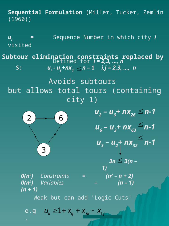
Sequential Formulation (Miller, Tucker, Zemlin (1960))
ui = Sequence Number in which city i visited
Defined for i = 2,3, …, nSubtour elimination constraints replaced by
S: ui - uj +nxij n – 1 i,j = 2,3, …, n
Avoids subtours but allows total tours (containing city 1)
62
3
Weak but can add 'Logic Cuts'
u2 – u6+ nx26
n-1
u6 – u3+ nx63
n-1
u3 – u2+ nx32
n-1 3n 3(n – 1)
0(n2) Constraints = (n2 – n + 2)0(n2) Variables = (n – 1) (n + 1)
e.g. 11k ij jk ju x x x
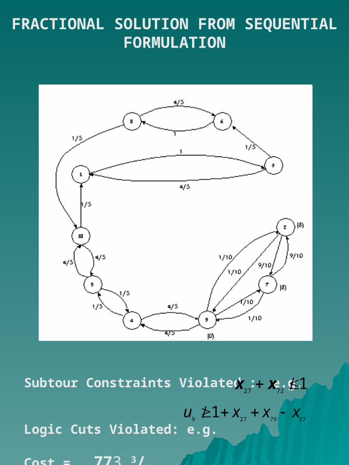
FRACTIONAL SOLUTION FROM SEQUENTIAL FORMULATION
Subtour Constraints Violated : e.g.
Logic Cuts Violated: e.g.
Cost = 773 3/5 (Optimal Cost = 881)
17227 xx
17792791 xxxu
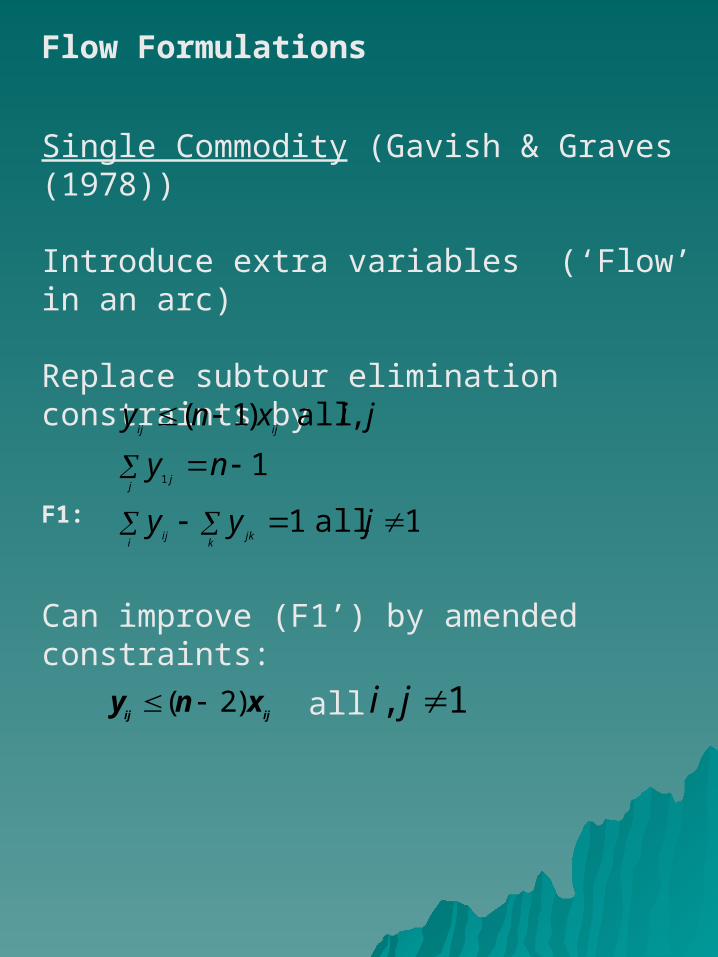
Flow Formulations
Single Commodity (Gavish & Graves (1978)) Introduce extra variables (‘Flow’ in an arc) Replace subtour elimination constraints by
F1:
1 all 1
1
, all )1(
1
jyy
ny
jixny
kjk
iij
jj
ijij
Can improve (F1’) by amended constraints:
ijijxny )2(
1, jiall
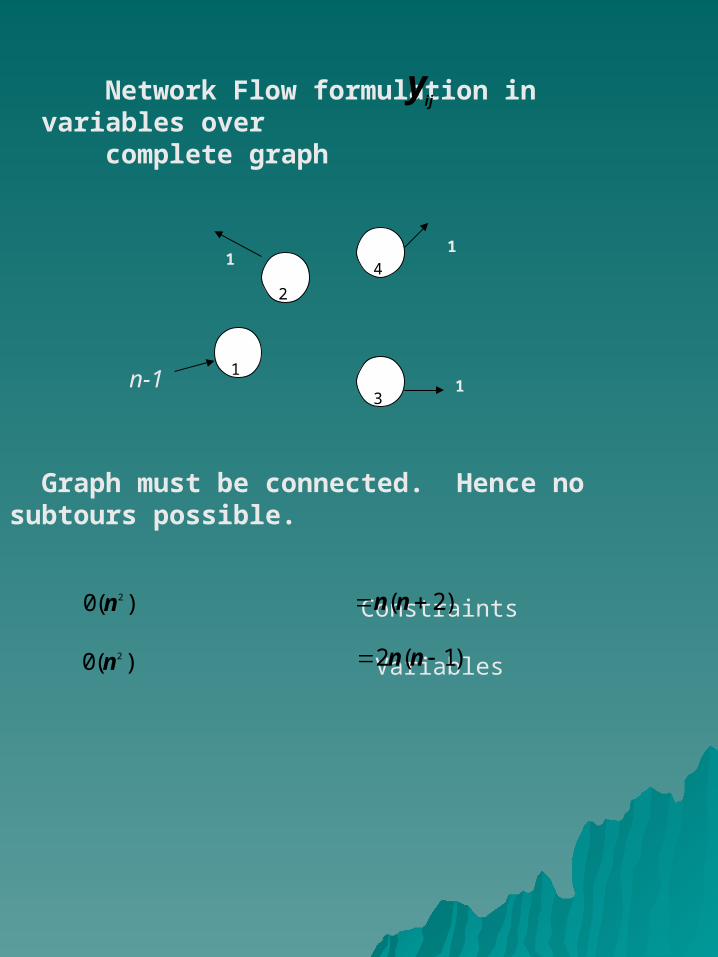
Network Flow formulation in variables over complete graph
ijy
4
2
1
3 1
1 1
Graph must be connected. Hence no subtours possible.
Constraints Variables
)(0 2n )2( nn
)(0 2n )1(2 nn
n-1
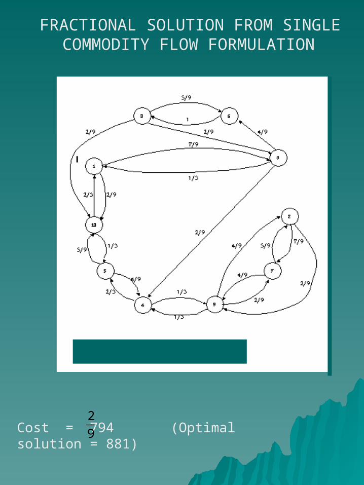
FRACTIONAL SOLUTION FROM SINGLE COMMODITY FLOW FORMULATION
Cost = 794 (Optimal solution = 881) 2
9
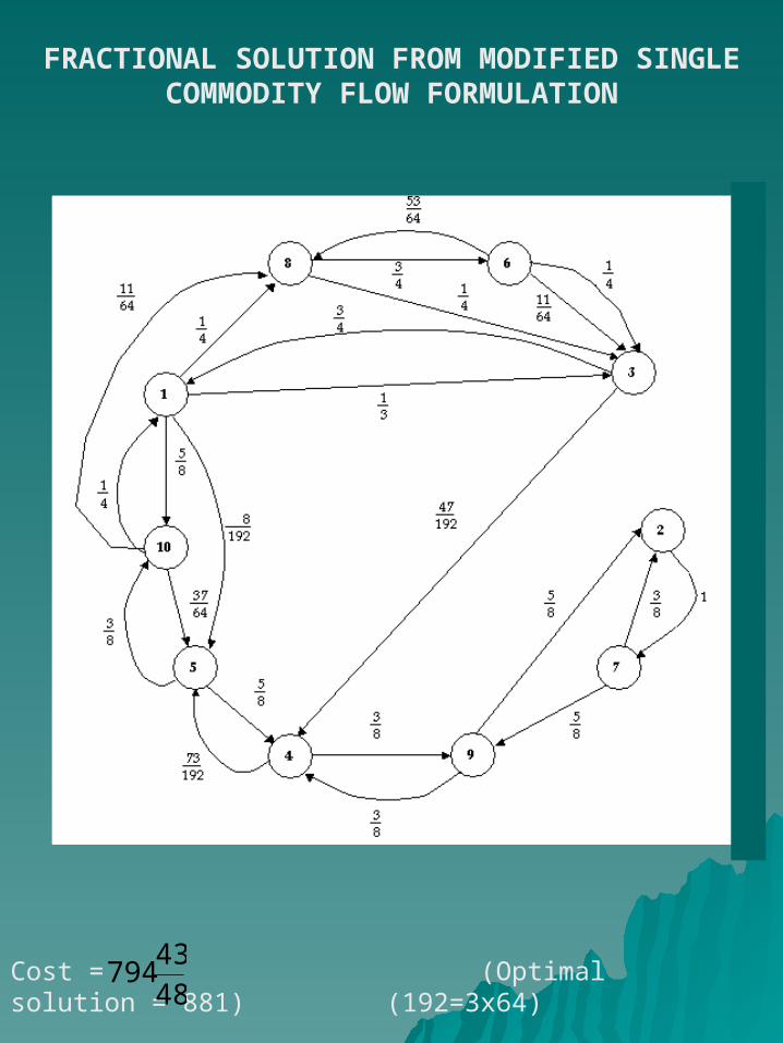
FRACTIONAL SOLUTION FROM MODIFIED SINGLE COMMODITY FLOW FORMULATION
Cost = (Optimal solution = 881) (192=3x64)
48
43794

Two Commodity Flow (Finke, Claus Gunn (1983))
jiz
jiy
ij
ij
arcin 2commodity of flow is
arcin 1commodity of flow is
j
jij
ijyy
11
11
in
i
j
jij
ijzz
1)1(
11
in
i
j
jij
ijzz 1 all n i
ijijzy ( 1) all ,ijn x i j
=
=
F2:
1 2
3
1
1
1 Commodity 2 1
)(0 2n )4( nn
)(0 2n )1(3 nnVariables
Constraints
n-1
Commodity 1Commodity 2n-1
Commodity 1
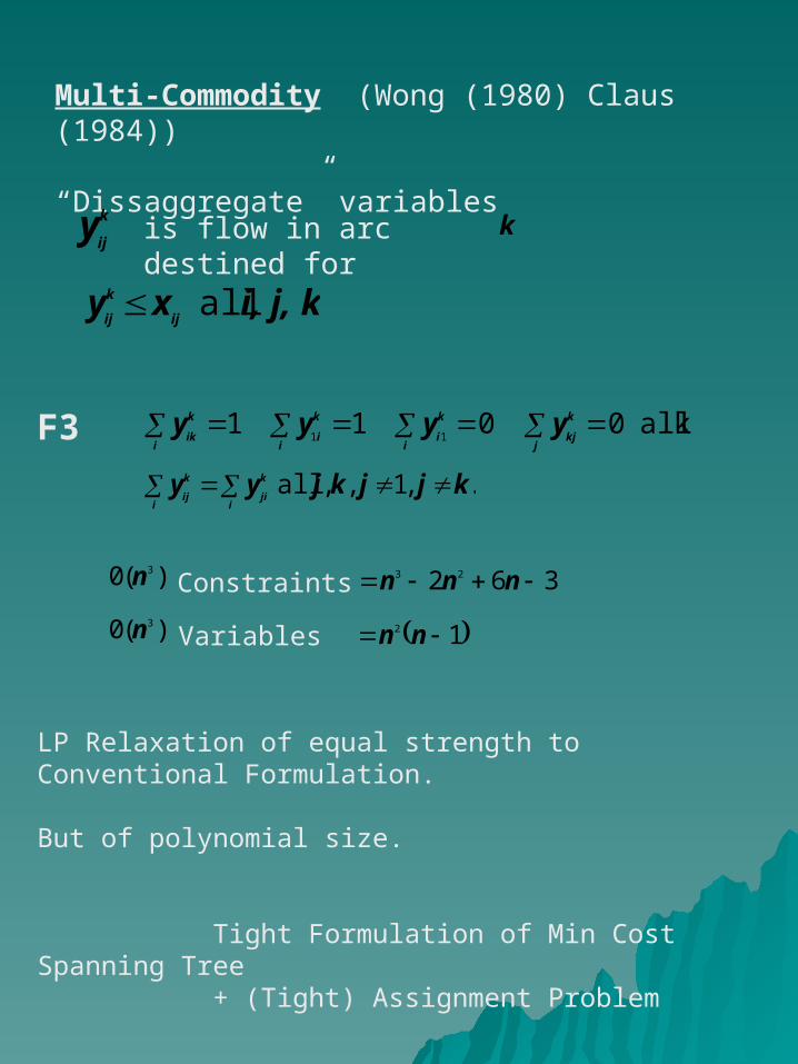
Multi-Commodity (Wong (1980) Claus (1984)) “Dissaggregate” variables
k
ijy is flow in arc destined
for k
i, j, kxyij
k
ij all
k all001111
j
k
kji
k
ii
k
ii
k
ikyyyyF3
.,1,, all kjjkjyyi
k
jii
k
ij
)(0 3n 362 23 nnn
)(0 3n 12 nn Variables
Constraints
LP Relaxation of equal strength to Conventional Formulation. But of polynomial size. Tight Formulation of Min Cost Spanning Tree + (Tight) Assignment Problem
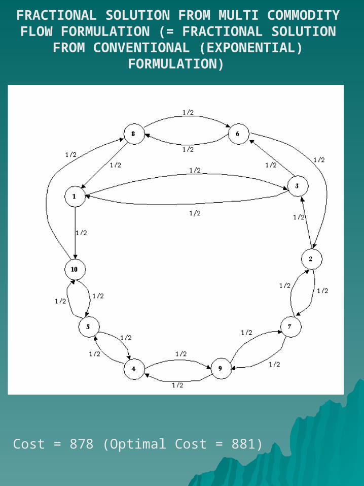
FRACTIONAL SOLUTION FROM MULTI COMMODITY FLOW FORMULATION (=
FRACTIONAL SOLUTION FROM CONVENTIONAL (EXPONENTIAL) FORMULATION)
Cost = 878 (Optimal Cost = 881)
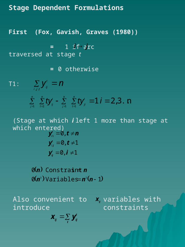
Stage Dependent Formulations First (Fox, Gavish, Graves (1980))
= 1 if arc traversed at stage t
= 0 otherwise T1:
ji
nytji
t
ij
,,
n...3,211121
itytyn
t
t
ji
n
j
n
t
t
ij
n
j
1,0
1,0
,0
1
1
1
iy
ty
nty
ij
t
j
t
i
1Variables0
sConstraint023
nnn
nn
(Stage at which i left 1 more than stage at which entered)
t
t
ijijyx
Also convenient to introduce ijx variables with constraints
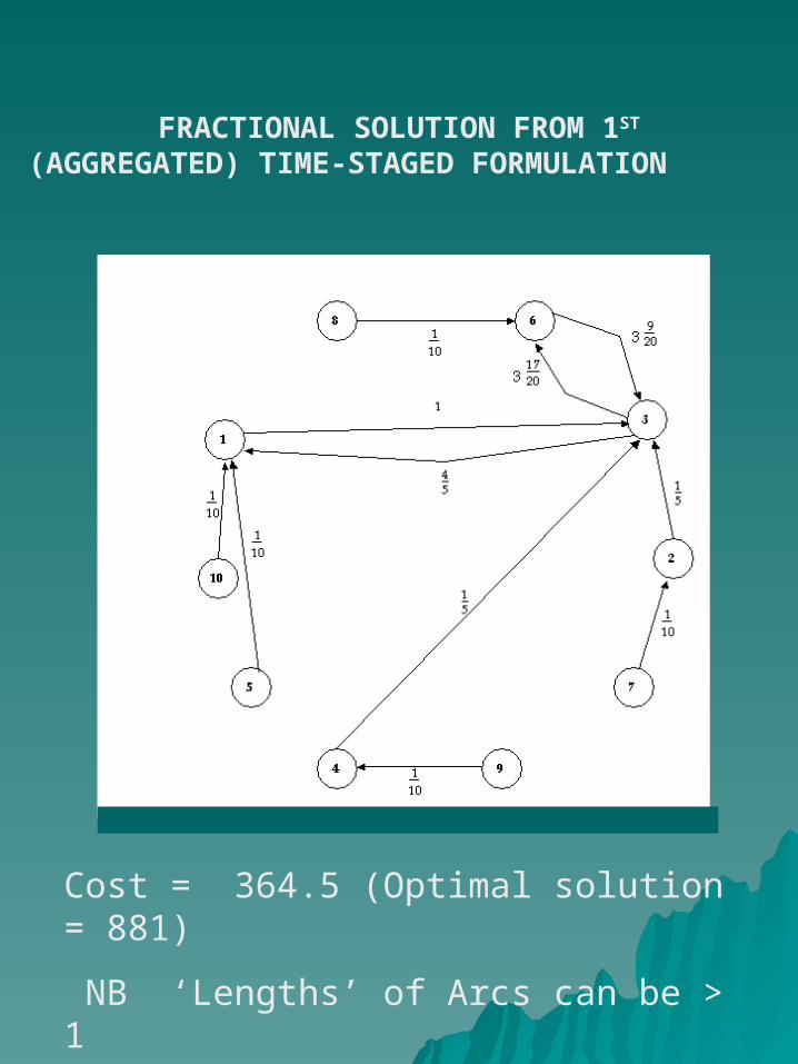
FRACTIONAL SOLUTION FROM 1ST (AGGREGATED) TIME-STAGED FORMULATION
Cost = 364.5 (Optimal solution = 881)
NB ‘Lengths’ of Arcs can be > 1
1,
tij
tji
y
1,
tij
tij
y
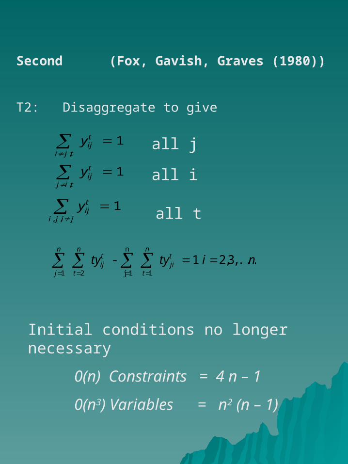
Second (Fox, Gavish, Graves (1980))
T2: Disaggregate to give
all j
all i
all t
nityty tji
n
t
tij
n
t
n
j
... ,3,2 1 - 1
n
1j21
Initial conditions no longer necessary
0(n) Constraints = 4 n – 1
0(n3) Variables = n2 (n – 1)
1,,
tij
jiji
y
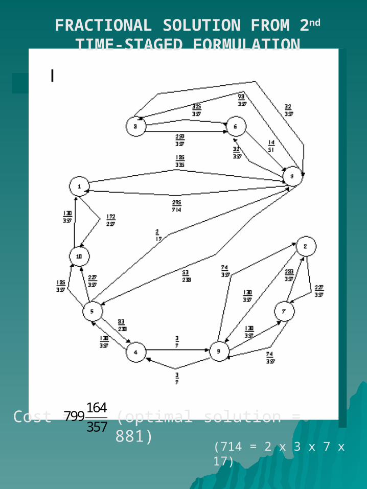
FRACTIONAL SOLUTION FROM 2nd TIME-STAGED FORMULATION
Cost =164
799357
(optimal solution = 881)
(714 = 2 x 3 x 7 x 17)
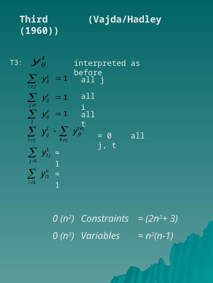
Third (Vajda/Hadley (1960))
T3:
tijy interpreted as
before 1
tij
ji
y all j
1
tij
ij
y all i
1 tij
t
y all t
t
ijji
y
1
t
jkjk
y= 0 all j, t
11
1j
j
y
= 1
ni
i
y 11
= 1
0 (n2) Constraints = (2n2+ 3)
0 (n3) Variables = n2(n-1)
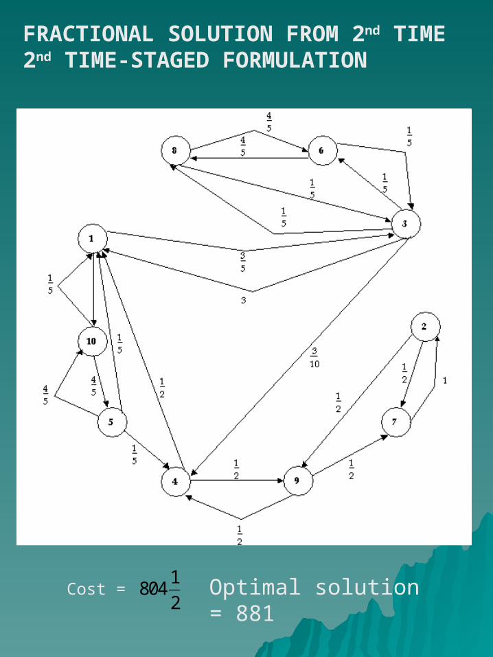
FRACTIONAL SOLUTION FROM 2nd TIME 2nd TIME-STAGED FORMULATION
Cost =1
8042
Optimal solution = 881
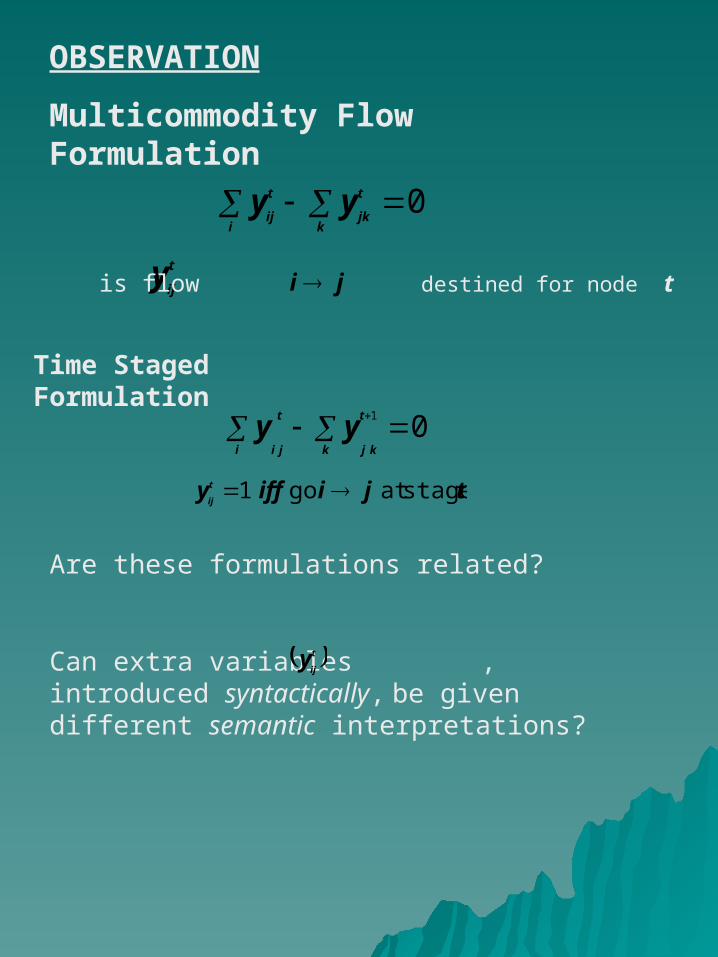
OBSERVATION
Multicommodity Flow Formulation
0k
t
jki
t
ijyy
t
ijy ji is flow destined for node t
Time Staged Formulation
01
t
kjk
t
jii
yy
tjiiffy t
ij stageat go1
Are these formulations related?
Can extra variables , introduced syntactically, be given different semantic interpretations?
t
ijy
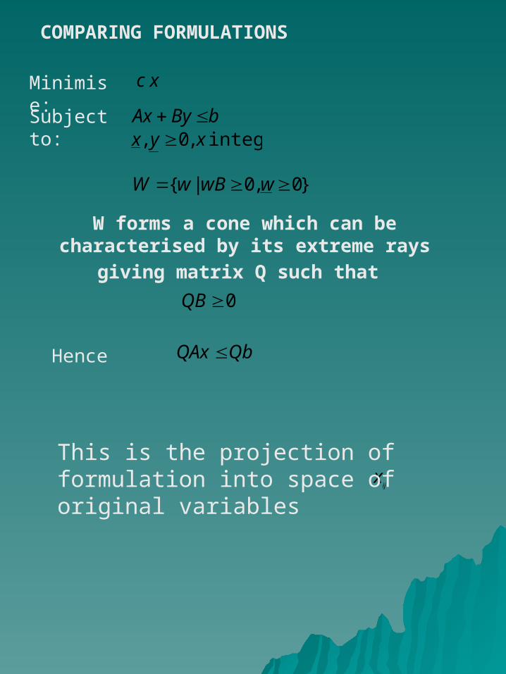
COMPARING FORMULATIONS
Minimise:
c x
Subject to:
bByAx integer ,0 , xyx
}0,0|{ wwBwW
W forms a cone which can be characterised by its extreme rays
giving matrix Q such that 0QB
QbQAx Hence
ijx
This is the projection of formulation into space of original variables
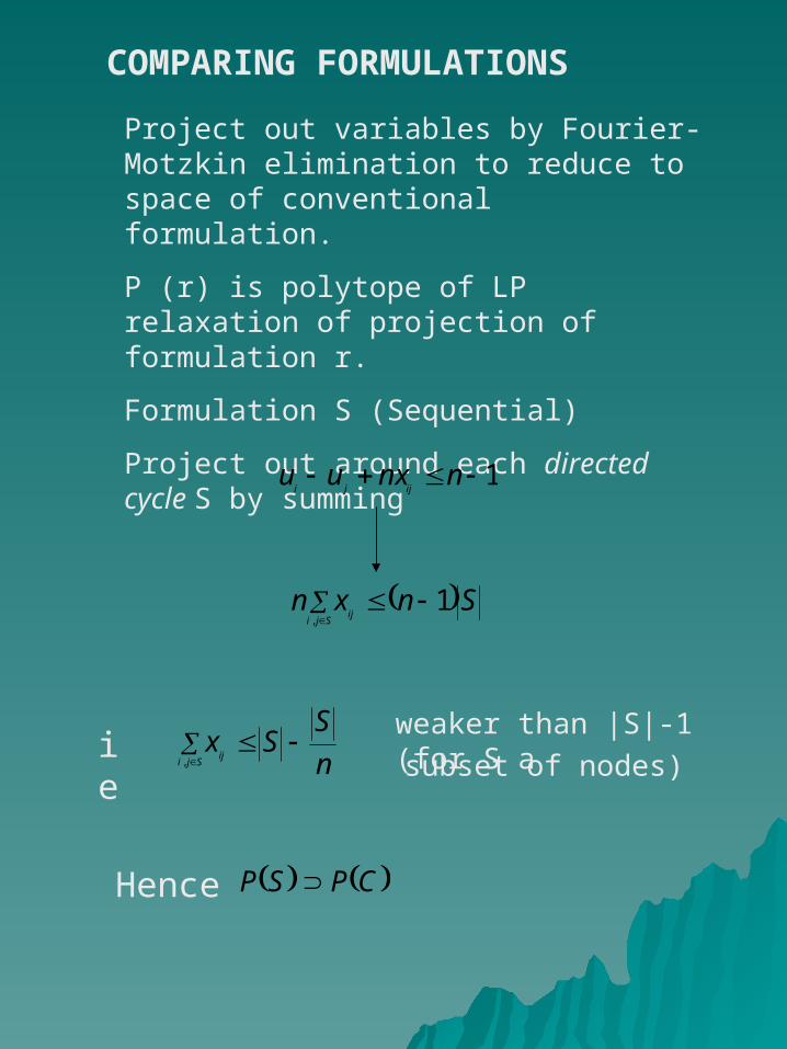
COMPARING FORMULATIONS
Project out variables by Fourier-Motzkin elimination to reduce to space of conventional formulation.
P (r) is polytope of LP relaxation of projection of formulation r.
Formulation S (Sequential)
Project out around each directed cycle S by summing
1 nnxuuijji
SnxnSji
ij1
,
ie n
SSx
Sjiij
,
weaker than |S|-1 (for S asubset of nodes)
Hence CPSP
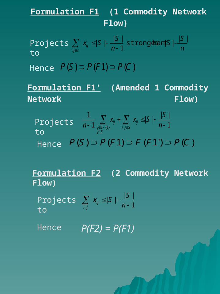
Formulation F1 (1 Commodity Network Flow)
n
|| - |S|han stronger t
1
||||
S
n
SSxij
sij
Projects to
)()1()( CPFPSP Hence
Formulation F1' (Amended 1 Commodity Network
Flow)
1
||||
1
1
,}1{
n
SSxx
n ijSji
ij
SjSj
Projects to
Hence )()'1()1()( CPFFFPSP
Formulation F2 (2 Commodity Network Flow)
Projects to 1
||||
, n
SSxij
ji
Hence P(F2) = P(F1)
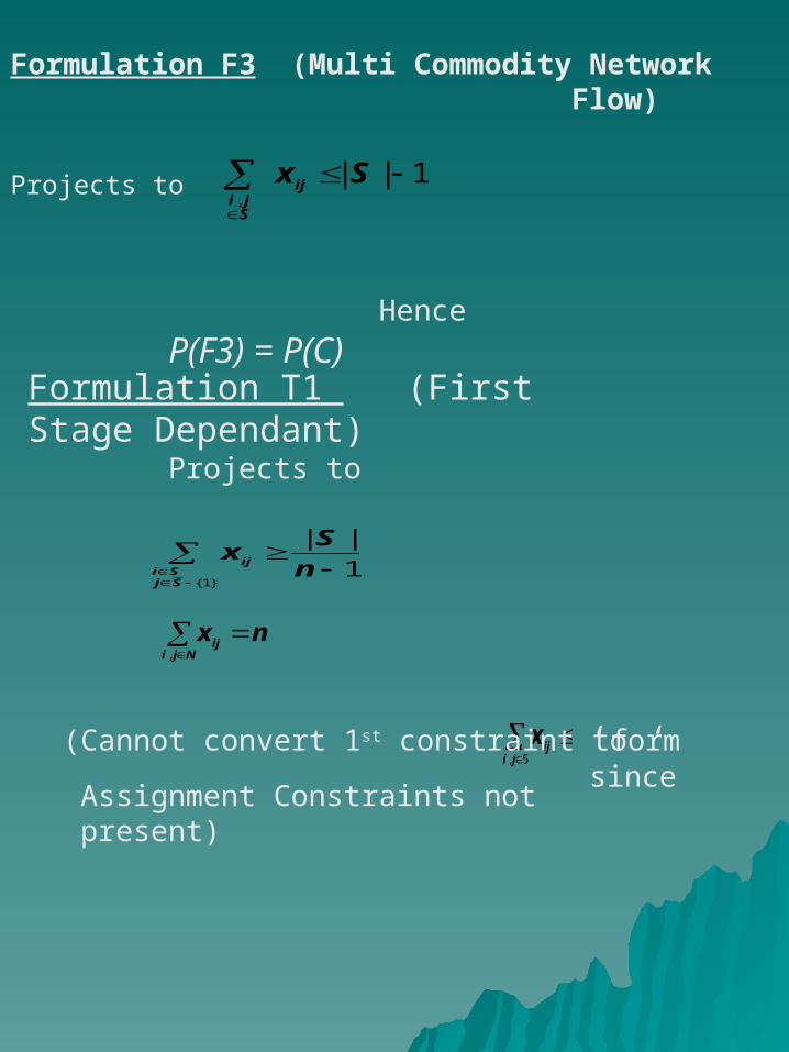
Formulation F3 (Multi Commodity Network Flow)
Projects to 1||
,
Sx ij
Sji
Hence P(F3) = P(C)
Formulation T1 (First Stage Dependant)
Projects to
1
||
}1{
n
Sxij
SjSi
nxNji
ij ,
5, ji
ijx(Cannot convert 1st constraint to ‘ ‘form since
Assignment Constraints not present)
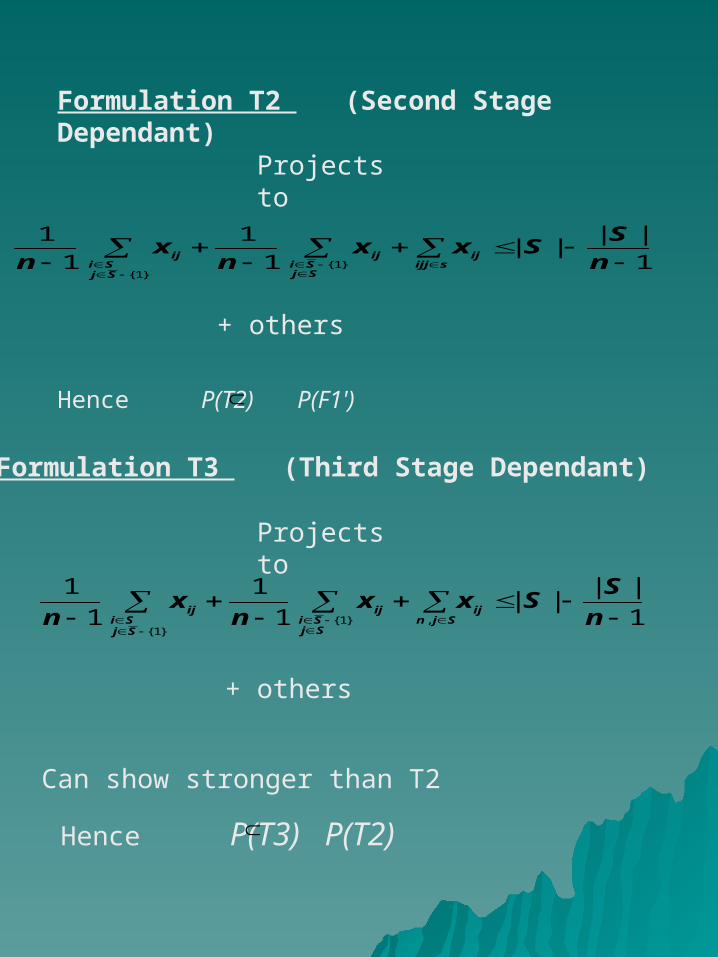
Formulation T2 (Second Stage Dependant)
Projects to
1
||||
1
1
1
1}1{
}1{
n
SSxx
nx
n sijjijij
SjSi
ij
SjSi
Hence P(T2) P(F1')
+ others
Formulation T3 (Third Stage Dependant)
Projects to
1
||||
1
1
1
1,}1{
}1{
n
SSxx
nx
n Sjnijij
SjSi
ij
SjSi
+ others
Can show stronger than T2
Hence P(T3) P(T2)
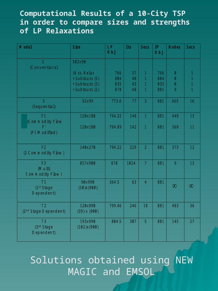
M o d e l S iz e L P O bj
I t s S e c s I P O bj
N o d e s S e c s
C (C on v en tion al
502x90 (A ss. R elax +Su btou rs (5) +Su btou rs (3) +Su btou rs (2)
766 804 835 878
37 40 43 48
1 1 1 1
766 804 835 881
0 0 0 9
1 1 1 1
S (Sequ en tial )
92x99 773.6 77 3 881 665 16
F 1 1(C om m od i ty F low
F ' (F 1 M od ifi ed )
120x180
120x180
794.22
794.89
148
142
1
1
881
881
449
369
13
11
F 2 (2 C om m od i ty F low )
140x270 794.22 229 2 881 373 12
F 3 (M u l ti
C om m od i ty F low )
857x900 878 1024 7 881 9 13
T 1 (1st Stage
D ep en d en t)
90x990 (10)x(900)
364.5 63 4 881
T 2 (2n d Stage D ep en d en t)
120x990 (39) x (900)
799.46 246 18 881 483 36
T 3 (3rd Stage
D ep en d en t)
193x990 (102)x(900)
804.5 307 5 881 145 27
Computational Results of a 10-City TSP in order to compare sizes and strengths of LP Relaxations
Solutions obtained using NEW MAGIC and EMSOL
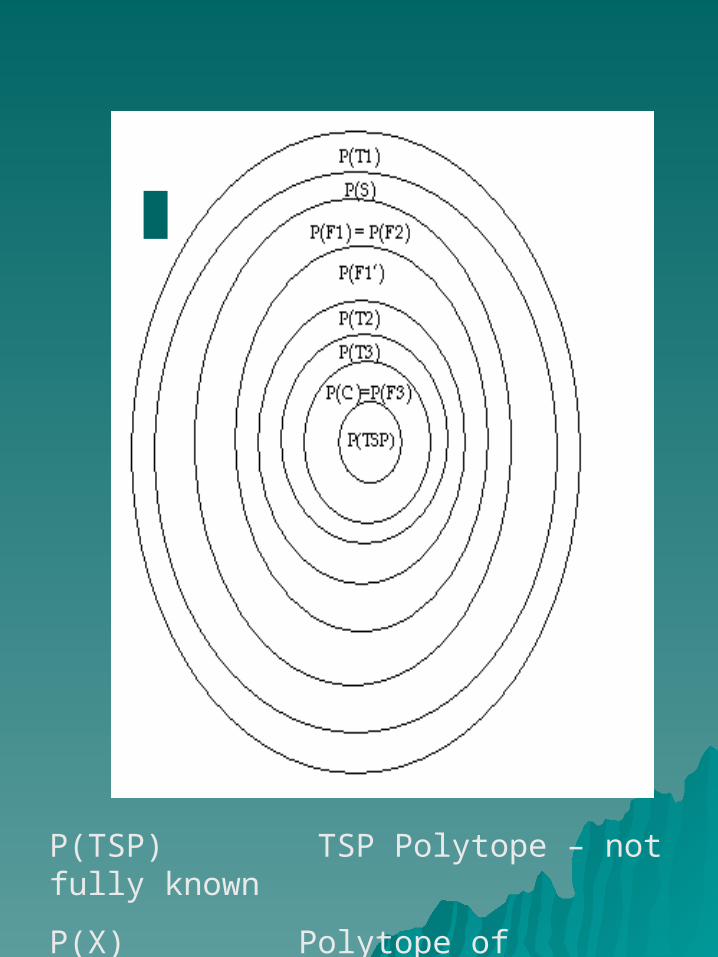
P(TSP) TSP Polytope – not fully known
P(X) Polytope of Projected LP relaxations
ReferenceReference
AJ Orman and HP Williams,AJ Orman and HP Williams,
A Survey of Different Formulations of the A Survey of Different Formulations of the Travelling Salesman Problem, Travelling Salesman Problem,
in C Gatu and E Kontoghiorghes (Eds),in C Gatu and E Kontoghiorghes (Eds), Advances in Computational Management Advances in Computational Management Science 9 Optimisation, Econometric and Science 9 Optimisation, Econometric and Financial Analysis (2006) SpringerFinancial Analysis (2006) Springer