Errata

Title & Document Type:

Manual Part Number:

Revision Date:

HP References in this Manual This manual may contain references to HP or Hewlett-Packard. Please note that Hewlett-Packard's former test and measurement, semiconductor products and chemical analysis businesses are now part of Agilent Technologies. We have made no changes to this manual copy. The HP XXXX referred to in this document is now the Agilent XXXX. For example, model number HP8648A is now model number Agilent 8648A.

About this Manual We’ve added this manual to the Agilent website in an effort to help you support your product. This manual provides the best information we could find. It may be incomplete or contain dated information, and the scan quality may not be ideal. If we find a better copy in the future, we will add it to the Agilent website.

Support for Your Product Agilent no longer sells or supports this product. You will find any other available product information on the Agilent Test & Measurement website:

www.tm.agilent.com Search for the model number of this product, and the resulting product page will guide you to any available information. Our service centers may be able to perform calibration if no repair parts are needed, but no other support from Agilent is available.

" "

rj3'HEWLETT~~ PACKARD

r~.

"

.

..'

,"} CHAPTER 1

Basic Considerations

Definition of SensitivitySensitivity, to be useful, needs to relate to how small a signal can be measured on the analyzer. The

CRTdeflection is always proportional to the total power which includes the signal and the noise. A signalcan be seen when it is equal to the noise power.

S+NS=Nor-=2 NS = power of the signalN = power of the noise

(1), where

In this case, S + N will be twice the noise power or deflected 3 dB above the noise.

Available Noise Power

The input termination of a network (an amplifier, receiver, or spectrum analyzer) has a certain amountof available noise power which is, in most cases, thermal noise. An impedance Z = R + jX at temperatureT generates across its open circuit terminals a voltage resulting from the random motion of free electronsthermally agitated. This "noise voltage", en, can be defined by the equation:

J- ",~

en: = 4kTBR,where

k = Boltzmann's constant 1.374x 10-23joule/oKT = absolute temperature oKR = resistive component of impedanceB=Bandwidth

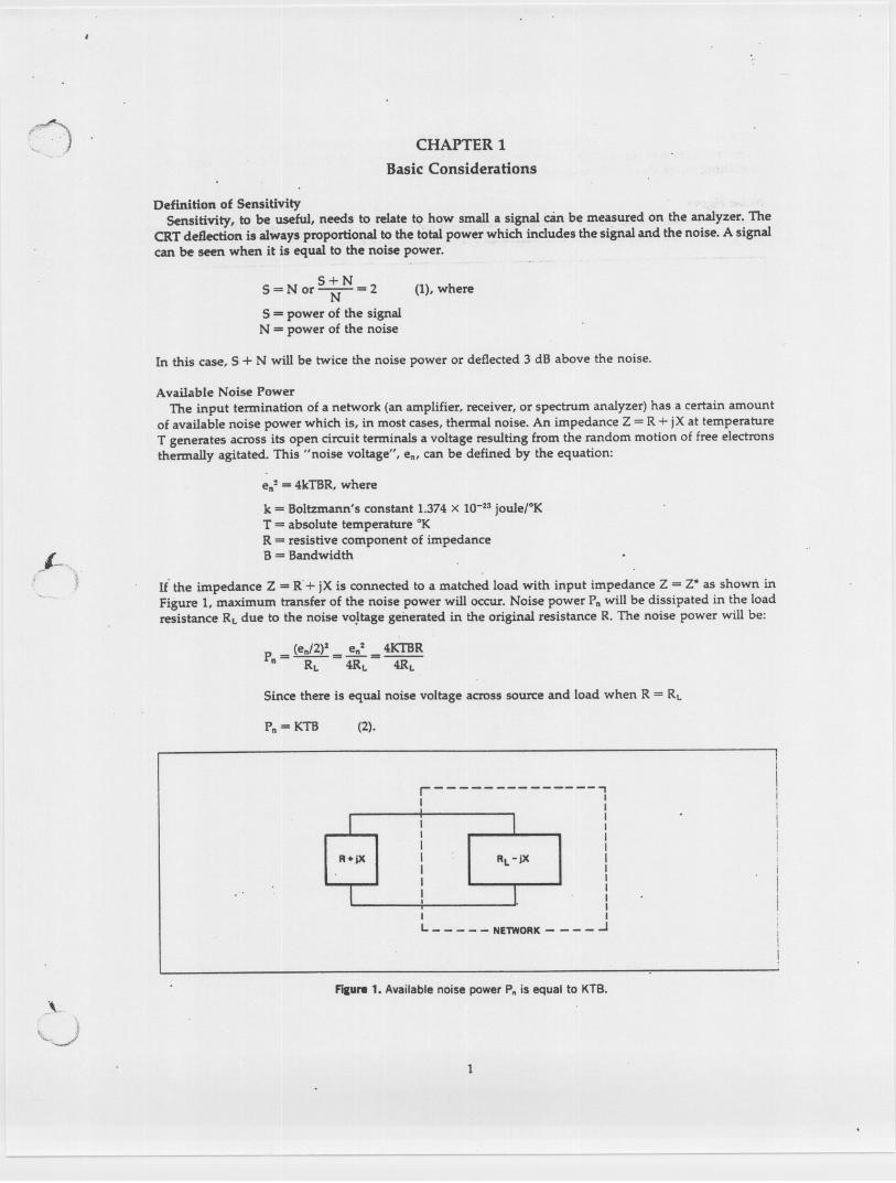
If the impedance Z = R.+ jX is connected to a matched load with input impedance Z = Z. as shown inFigure 1, maximum transfer of the noise power will occur. Noise power Pn will be dissipated in the loadresistance RLdue to the noise voJtage generated in the original resistance R. The noise power will be:

P = (en/2)2 =~ = 4KTBRn RL 4RL 4RL

Since there is equal noise voltage across source and load when R = RL

Pn = KTB (2).

R+jX

r 'I II

IIIIIIIIII

I IL - - - - - NETWORK - - - - .J

RL -jX

Filure 1. Availablenoise power P. is equal to KTB.

_\"

.~ y

1

.-Equation (2) defines the available noise power from the source. In systems operating at frequencies

where voltages and resistances cannot be clearly defined, this equation becomes the usable expression,containing terms that can be measured.

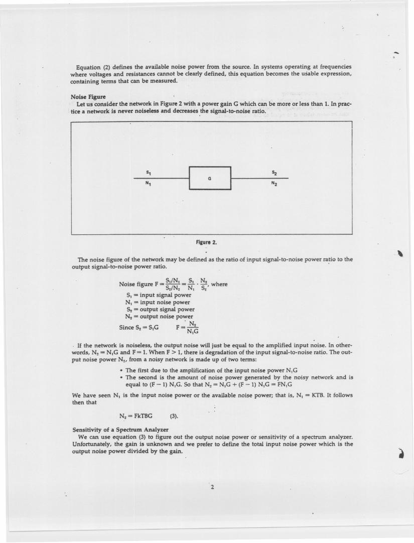
Noise FigureLet us consider the network in Figure 2 with a power gain G which can be more or less than 1. In prac-

tice a network is never noiseless and decreases the signal-to-noise ratio.

St ~G

N, N2

Fillure2.

The noise figure of the network may be defined as the ratio of input signal-to-noise power ratio to theoutput signal-to-noise power ratio. .

.~

. fi F StiNt St N2NOIse gure =-=-'-,where

~/N2 Nt 52St = input signal powerNt = input noise power~ = output signal power

N: = output noise power'N

Since ~ = StG F = Nt~

. H the network is noiseless, the output noise will just be equal to the amplified input noise. In other-words, N2 =NtG and F= 1. When F > I, there is degradation of the input signal-to-noise ratio. The out-put noise power Nt, from a noisy network is made up of two terms:

. The first due to the amplification of the input noise power N.G.The second is the amount of noise power generated by the noisy network and isequal to (F - 1) N,G. So that Nt = N.G + (F- 1) N.G = FN.G

We have seen Nt is the input noise power or the available noise powj!r; that is, Nt = KTB. It followsthen that

Nt = FkTBG (3).

Sensitivity of a Spectrum AnalyzerWe can use equation (3) to figure out the output noise power or sensitivity of a spectrum analyzer.

Unfortunately, the gain is unknown and we prefer to define the total input noise power which is theoutput noise power divided by the gain. .

2

~

t-"'."-~

,-

\.,-.J

j

Equation (3) becomes

N = FsAkTB (4) with FSA= Spectrum analyzer noise figure.

x;:.' It's more convenient to express the formula in dB

10 log N = 10 log FSA+ 10 log kT + 10 log B

At room temperature, T = 290okand 10log KT= -204 dB,a value which is constant in normal utilization.(VVehave an error of 0.4 dB for t = 23°C:t:30°C.)Units are usually expressed in dBm, that is dB referredto a mW. Since 0 dBm = 1 mW, we get .

(N)dBm = (FsA)dB + (B)dB - 174 dBm (5), where.

(FsA)dBis the noise figure of the spectrum analyzer in dB, (B)dB= 10 log B where B is theequivalent noise power bandwidth in Hz (in gaussian filters this is 1.2 times the resolu-tion bandwidth). For simplicity this applications note will use the analyzers bandwidthsetting for B. Thus if B= 1 Hz, then 10 log B= 0 or if B = 10 kHz, then 10 log B= 40 dB.

A 10 times increase in the bandwidth causes the spectrum analyzer internal noise to increase by 10 dB.For instance, if the internal noise power is -110 dBm with 10 KHz BW;

at 1 KHz IF, we get -120 dBm;. at 100 Hz IF, -130 dBm;

and so on.

Qbviously the sensitivity will be the best when the bandwidth is the narrowest.There is a restriction to this general comment for impulse noise measurements. In this particular case,

the maximum achievable measurement range is for the largest bandwidth. For more information, refer toHP Application Note 150-4: "SPECTRUM ANALYSIS. . . . Noise Measurements."

Average Noise LevelWe have seen that the sensitivity of a spectrum analyzer is a function of its internal noise which in

turn is related to its bandwidth. When the signal is equal to the noise power, the signal is deflected 3 dBabove the noise level since the analyzer always displays S + N. So one way to measure sensitivity wouldbe to insert a signal and decrease its level until it is 3 dB above the noise.

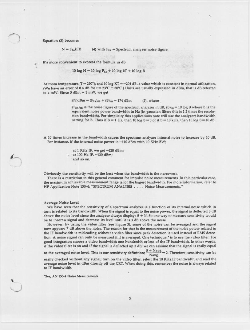
However, by using the video filter (see Figure 3), some of the noise can be averaged and the signalnow appears 7 dB above the noise. The reason for that is the measurement of the noise power related tothe IF bandwidth is misleading without a video filter since peak detection is used instead of RMS detec-tion. A noise signal can only be measured if it is averaged. One technique," is to use the video filter. Forgood integration choose a video bandwidth one hundredth or less of the IF bandwidth. In other words,if the video filter is on and if the signal is deflected up 3 dB, we can assume that the signal is really equal

th ed '. I I Th . . . .. d f. .. S + Navg 2 Th f . . . bto e averag nOise eve. IS ISour sensitivity e lmhon; N . ere ore, senslhvlty can e. avg

easily checked without any signal; turn on the video filter, select the 10 KHz IF bandwidth and read theaverage noise level in dBm directly off the CRT. When doing this, remember the noise is always relatedto IF bandwidth.

"See, AN 150-4 Noise Measurements

3

--- --~------------

-,-410..

Filure 3.Thesame signal power is displayed without video filter in left photo and after averaging (10 Hz videofilter) in right photo.

Spectrum Analyzers, with High ImpedanceSo far the spectrum analyzer's noise figure has been determined from the available noise power since

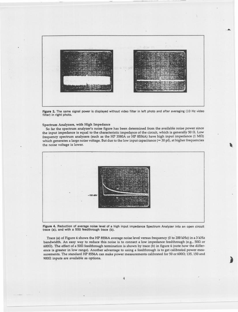
the input impedance is equal to the characteristic impeda,nce of the circuit, which is generally 50 il. Lowfrequency spectrum analyzers (such as the HP 3580A or HP 8556A) have high input impedance (1 Mil)which generates a large noise voltage. But due to the low input capacitance (= 30 p£), at higher frequenciesthe noise voltage is lower. \

-11OdBV

Figure 4. Reduction IJf average noise level of a high input impedance Spectrum Analyzer into an open circuittrace (a),- and with a 500 feedthrough trace (b).

,Trace (a) of Figure 4 shows the HP 8556A average noise level versus frequency (0 to 200 kHz) in a 3 kHzbandwidth. An easy way to reduce this noise is to connect a low impedance feedthrough (e.g., SOil or6OOil).The effect of a SOil feedthrough termination is shown by trace (b) in figure 4 (note how the differ-ence is greater in low range). Another advantage to using a feedthrough is to get calibrated power mea-surements. The standard HP 8556A can make power measurements calibrated for 50 or 600!1; 135, 150and9OOil inputs are available as options.

)

4

I"A~

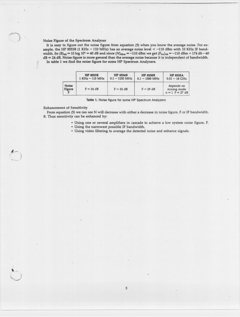
) . Noise Figure of the Spectrum AnalyzerIt is easy to figure out the noise figure from equation (5) when you know the average noise. For ex-

ample, the HP 8553B (1 KHz - 110 MHz) has an average noise level < -110 dBm with 10 KHz IF band-width. So (B)dB=10 log 10. =40 dB and since (N)dBm=-110 dBm we get (Fs.JdB=-110 dBm + 174 db-4OdB = 24 dB. Noise figure is more general than the average noise because it is independent of bandwidth.

In table 1 we find the noise figure for some HP Spectrum Analyzers.H

J'

,.

Table 1. Noise figure for some HP Spectrum Analyzers

Enhancement of SensitivityFrom equation (5) we can see N will decrease with either a decrease in noise figure, F or IF bandwidth,

B. Thus sensitivity can be enhanced by:

.Using one or several amplifiers in cascade to achieve a low system noise figure, F..Using the narrowest possible IF bandwidth..Using video filtering to average the detected noise and enhance signals.

l~~

,..

~~

V

5

HP 8553B HP 8S54B HP 8558B HP 8SS5A1 KHz -110 MHz 0.1 - 1250 MHz 0.1 - 1500 MHz 0.01 - 18 GHz

Noise depends onFigure F = 24 dB F = 32 dB F =29 dB . mixing mode

F n = 1 F = 27 dB :I

.'

CHAPTER 2

Amplifiers and Sensitivity

The simplest method to handle weak signals is to connect a broadband amplifier at the input of thespectrum analyzer. In this chapter we are, going to define how much we can improve the sensitivity anddetermine the number of amplifiers we can connect in cascade for a maximum enhancement.

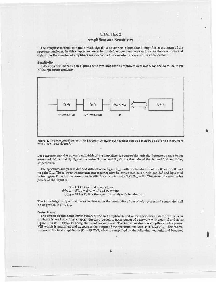
SensitivityLet's consider the set up in Figure 5 with two broadband amplifiers in cascade, connected to the input

of the spectrum analyzer.

--1F,.G, H FZ'Gz H '~&GSA 1< >G

,It AMPLIFIER znct AMPl.IFIER SA

,Figure 5. The two amplifiers and the Spectrum Analyzer put together can be considered as a single instrumentwith a new noise figure Ft.

Let's assume that the power bandwidth of the amplifiers is compatible with the frequency range beingmeasured. Note that FI, F2 are the noise figures and GI, G2 are the gain of the 1st and 2nd amplifier,respectively.

The spectrum analyzer is defined with its noise figure FSAIwith the bandwidth of the IF section B, andits gain GSA'These three instruments put together may be considered as a single one defined by a total,noise figure FI, with the same bandwidth B and a total gain GIG2GSA= GI. Therefore, the total noisepower at the input is: '

N = FII<TB(see first chapter), or(N)dBID= (FJdB+ (B)dB-174 dBm, where

(B)dB= 10 log B, B is the spectrum analyzer's bandwidth.

The knowledge of FI will allow us to determine the sensitivity of the whole system and sensitivity willbe improved if FI < FSA'

Noise FigureThe effects of the noise contribution of the two amplifiers, and of the spectrum analyzer can be seen

in Figure 6. We know (first chapter) the contribution to noise power of a network with a gain G and noisefigure F is (F - 1)NG, N being the input noise power. The input termination supplies a noise powerkTB which is amplified and appears at the output of the spectrum analyzer as kTBGIG2GSA'The contri-bution of the first amplifier is (FI - l)kTBGI which is amplified by the following networks and becomes

)-

6

----.

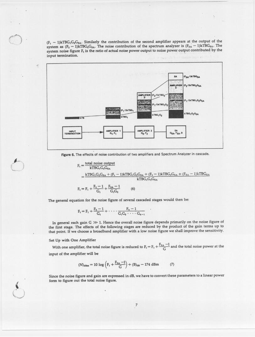
.~(~.~, ) (F, - l)kTBG,GzGsA. Similarly the contribution of the second amplifier appears at the output of the

system as (Fz - l)kTBGzGSA' The noise contribution of the spectrum analyzer is (Fs~ - l)kTBGsA.Thesystem noise figure F, is the ratio of actual noise power output to noise power output contributed by theinput termination. .

(.

kTB

SA

(F,,'JkT8G,G2GsA

kT8G,G2GSA

Figure6. The effects of noise contribution of two amplifiers and Spectrum Analyzer in cascade.

~,",

t«.A'"./FI= total noise output

. kTBGIGZGSA

- kTBG.GZGSA + (F. - l)kTBG,GzGSA + (Fz - l)kTBGzGsA + (FSA - l)kTBGsA- kTBG.GZGSA

Fz - 1 + FSA - 1F,=F, + GI GIGZ

(6)

The general equation for the noise figure of several cascaded stages would then be:

F - 1 Fn - 1F+ z + GFI = I ~ GIGZ . . .. n-I

In general each gain G » 1. Hence the overall noise figure depends primarily on the noise figure ofthe first stage. The effects of the following stages are reduced by the product of the gain terms up tothat point. If we choose a broadband amplifier with a low noise figure we shall improve the sensitivity.

Set Up with One Amplifier

With one amplifier, the total noise figure is reduced to FI= F, + Fs~-1 and t~e total noise power at the

input of the amplifier: will be

( FSA-1 )(N)dBm= 10 log F, + --c;- + (B)dB- 174 dBm (7)

(\..

{' "\

~J

Since the noise figure and gain are expressed in dB, we have to convert these parameters to a linear powerform to figure out the total noise figure.

7

INPUT AMPLIFIER' AMPLIFIER2 SATERMINATION -- 0,. F, Gz.F2 GsA. FSA' B

..EXAMPLE

With the HP 8553B (1 kHz -110 MHz and F =24 dB) we can use a broadband amplifier 8447A (F=5 dB;G =20 dB).

F = 24 dB is equivalent to F (linear) = 251,F = 5 dB is equivalent to F (linear) = 3.16,and G = 20 dB becomes G (linear)= 100. "';

251-1FI = 3.16 + 100 = 5.66 or 7.53 dB

and with a bandwidth of 10 Hz the noise power is

(N)dBm= 7.53dB + 10 dB - 174dBm=-156.47 dBm

At the same bandwidth the HP 8553B alone has an internal noise power of -140 dBm so we enhance thesensitivity by about +16 dB with an amplifier which has a gain of 20 dB. This is due to the noise contri-bution of-the amplifier. It would have been a mistake to believe that the sensitivity would increase by20 dB.

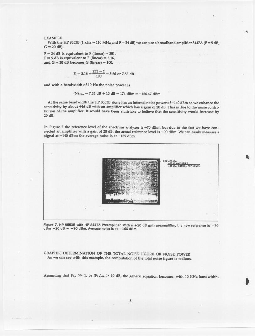
In Figure 7 the reference level of the spectrum analyzer is -70 dBm, but due to the fact we have con-nected an amplifier with a gain of 20 dB, the actual reference level is -90 dBm. We can easily measure asignal at -140 dBm; the average noise is at -155 dBm.

,REF -70 dBm

-20 dB AMPLI FI ER-90 dBm ACTUAL REF LEVEL

Figure 7. HP 8553B with HP 8447A Preamplifier. With a +20 dB gain preamplifier, the new reference is -70dBm -20 dB - -90 dBm. Average noise is at -160 dBm.

GRAPHIC DETERMINATION OF THE TOTAL NOISE FIGURE OR NOISE POWERAs we can see with this example, the computation of the total noise figure is tedious.

Assuming that FSA» 1, or (FSA)dB> 10 dB, the general equation becomes, with 10 KHz bandwidth,

t-

8

- -- ----

,C)"

,

O'

,

""

,

'

\ ' ,

'<"..",,-

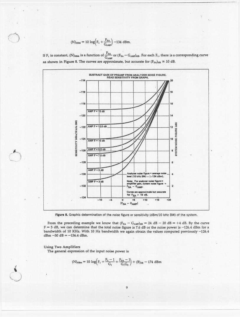
(N)dBm= 10log(Fl + ~:=J -134 dBm.

If Fl is constant, (N)dBmis a function of GFSA or (Fs~ - GAMP)dB'For each Fl, there is a corresponding curveAMP ,

as shown in Figure 8. The curves are approximate, but accurate for (FS.JdB2: 10 dB.

SUBTRACT GAIN OF PREAMP FROM ANAL VZER NOISE FIGURE.REAO SENSITIVITY FROM GRAPH.

-114

-118

~"""'"

("',I

~ noiI8 figu.. noiI8'-' (10 kHz BWI- (-134 dBmI.

Not8:For III8Iv- noiI8figure >ompIifi8r1IIin.syst8mnoiI8 figure ..FSA - GAMP.

eur- .. lII\WOXilll8l8but -.r8tIIfor FSA > 10 dB., . , .

0 +5 +10 +15 +20[FSA - GAMP)

14

CD...

12 ;;;II::I1:1;;:

10 ::«

(5z=:

8 =>en

8

4

2

FilUre 8. Graphic determination of the noise figure or sensitivity (dBm/10 kHz BW)of the system.

From the preceding example we know that (FSA- GAMP)dB = 24 dB - 20 dB = +4 dB. By the curveF = 5 dB, we can determine that the total noise figure is 7.6 dB or the noise power is -126.4 dBm for abandwidth of 10 KHz. With 10 Hz bandwidth we again obtain the values computed previously -126.4dBm -30 dB =-156.4 dBm.

Using Two AmplifiersThe general expression of the input noise power is

'0'"

(,J

( F2 - 1 FSA- I)(N)dBm= 10 log Fl + ~ + GlG2 + (B)dB- 174dBm

9

-118

IAMPF-ldB-120

i:2! -122...0

iCD3 -124 AMPF- 10dB

IIii -128 AMPF- 8.5dBZ'" AMPF-75dB'en

I-128

-130

F--132

-134-10 -6

~

,.>

where FI,F: are the linear noise figures and GI,G: are the linear power gains of the 1st and 2nd amplifiers.Calculation is always possible, but tedious. As a matter of fact, to enhance the sensitivity we have

to choose amplifiers with the largest gain and the lowest noise figure. If F~I~21 « 1 or (G1 + G:)dB

» (FS.JdBthe noise power is (N)dBm:.. 10 10g(F. + F2~ 1) -134 dBm with 10 KHz bandwidth, and thecurves of Figure aare helpful On the X axis we will have (F: - G1)dB and each curve is for (F.)dB con-stant. For example, with two amplifiers in cascade with 20 dB gain and 5 dB noise figure each, we have(F: - GI)dB =5 dB - 20 dB = -15 dB on the X axis and we get on the curve F. = 5 dB a sensitivity of-129dBm, i.e., 2.6 dB better than with a single amplifier. .

So the contribution of the second amplifier is poor; as a matter of fact, the total noise figure is 5 dBwith two amplifiers and 7.50 dB with a single amplifier. In practice with m:o amplifiers with low noisefigure and large gain (:2: 20 dB) the total noise figure is the noise figure of the first amplifier, and theconnection of a third one will contribute nothing since the total noise figure remains constant.

Maximum Input PowerBroadband amplifiers are specified for art output power with 1 dB gain compression. The HP 8447A

preamplifiers have < 1 dB compression for an output power of + 7 dBm; that means if the gain is + 20 dB,we cannot feed in a signal more than 7 dBm - 20 dB = -13 dBm in order to not compress the signal.

This may happen when you want to measure a weak signal present with a strong signal. Wheneverthe highest signal is compressed, the weak signal will be too. So before "zooming" in on the low signal,be sure that any strong signals won't overload the preamplifier.

On the other hand, if after preamplification, the signal fed to the spectrum analyzer is higher thanthe optimum input level, we have to adjust the input attenuator as we would if the spectrum analyzerwere used alone, since the output signal of the preamplifier may cause internal distortion.

Distortion

Amplifiers are never perfectly linear and we may have to worry about their harmonic distortion. For. example, let's compute the amplifier's contribution to an input signal's harmonic content. The HP 8447A

(+20 dB gain) has a typical harmonic distortion < -60 dB for < -30 dBm power output. Assume a signalwhose fundamental is at -50 dBm and second harmonic at -90 dBm. In theory, after amplification, thefundamental and the second harmonic would be respectively -30 dBm and -70 dBm. As a matter of fact,the actual amplitude of the 2nd harmonic is the result of two components, one due to the amplificationof the signal harmonic and the other due to the amplifier distortion. We know for an output power at-30 dBm the amplifier generates a second harmonic at -30 dBm - 60 dB = -90 dBm. Since the com-

ponents of the 2nd harmonic are coherent in phase we have to add the voltages; -70 dBm and -90 dBmcorrespond respectively to 70.7 Jl.Vand 7.07 Jl.Vin 50 n. Then the total voltage is 77.78 Jl.Vand the powerbecomes -69.17 dBm. So the second harmonic which was initially at-9O dBm is measured at-69.17 dBm- 20dB=89.17 dBm. So, due to the amplifier distortion we get an error of 0.83 dB.

."

Amplitude Accuracy and Adjustment of the New Reference LevelWhen you connect an amplifier to the spectrum analyzer the amplitude accuracy is degraded due to

the gain accuracy and the gain flatness of the amplifier. The total degradation of the accuracy is merelythe sum of the gain accuracy and gain flatness of the amplifier.

For example, with the HP 8447D Preamplifier the gain. is +26 dB ::!:1.5 dB and with a gain flatnessacross full frequency range at::!: 1.5 dB. Thus, the amplitude accuracy is degraded by::!: 3 dB.

To cancel the amplifier gain accuracy, we can calibrate the Spectrum Analyzer and amplifier connectedtogether, using the Spectrum Analyzer's internal calibrator. In our example, the degradation of the ampli-tude accuracy will decrease to ::!:1.5 dB.

As shown below this calibration will allow us to set the new reference level at an integral multipleof 10.

Let us consider the HP 8447D Preamplifier connected to the HP 8554B. After setting the input atten-uator (20 dB) to not overload the input mixer, connect the internal calibrator (30 MHz; - 30 dBm) and setthe log reference of the IF section to 0 dBm.

t.

10

(.) Let's assume the actual amplifier gain is +25 dB instead of the nominal +26 dB. To set the top of thedisplayed spectral line on a main division, we adjust the gain vernier to -5 dB. So t1i.eactual referencebecomes 0 dBm - 25 dB - 5 dB =-30 dBm. To figure out the new reference it will be sufficient to subtract-3O'dB frOm the reference level read from the knob. For example,

0 dBm corresponds to -30 dBm+ 10dBm corresponds to -20 dBm-10 dBm corresponds to -40 dBm and so on.

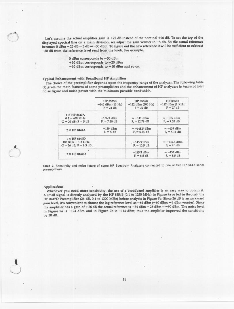
Typical Enhancement with Broadband HP AmplifiersThe choice of the preamplifier depends upon the frequency range of the analyzer. The following table

(2) gives the main features of some preamplifiers and the enhancemen't of HP analyzers in terms of totalnoise figure and noise power with the minimum possible bandwidth. '

HP 85S3B i HP 8554B HP 8558B i-140 dBm (10Hz) I

I

-122 dBm (100 Hz) i -117 dBm (1 KHz) :F = 24 dB F = 32 dB ' F = 27 dB

1 x HP 8447A0.1- 400 MHz

I G = 20 dB; F = 5 dB

2 x HP 8447A -159 dBmF. = 5 dB

-156.5 dBmF. = 7.50 dB

L(' ')"' j'

1 x HP 84470 I100 KHz - 1.3GHz i

G = 26dB; F = 8.5 dB :

2 x HP.84470

Table 2. Sensitivity and noise figure of some HP Spectrum Analyzers connected to one or two HP 8447 serialpreamplifiers.

ApplicationsWhenever you rieed more sensitivity, the use of a broadband amplifier is an easy way to obtain it.

A small signal is directly analyzed by the HP 8554B (0.1 to 1250 MHz) in Figure 9a or fed in through theHP 84470 Preamplifier (26 dB, 0.1 to 1300 MHz) before analysis in Figure 9b. Since 26 dB is an awkwardgain level, it's convenient to choose the log reference level as -64 dBm (-60 dBm; -4 dBm vern.ier). Sincethe amplifier has a gain of + 26 dB the actual reference is -64 dBm- 26dBm=-90 dBm. The noise levelin Figure 9a is -124 dBm and in Figure 9b is -144 dBm; thus the amplifier improved the sensitivityby 20 dB.

t",.>. ..

)~J

11

'" -141 dBm I '" -135 dBmIF. = 12.78 dB i F. =9.20 dB

,I

'" -148.5 dBm = -139 dBmF.= 5.24dB ! F,= 5.14dB

i,

, -143.5' dBm I '" -135.5 dBmF.= 10.5dB i F,= 9.1dB

'1-145.5 dBm i '" -136 dBmF,= 8.5dB I F,= 8.5 dB

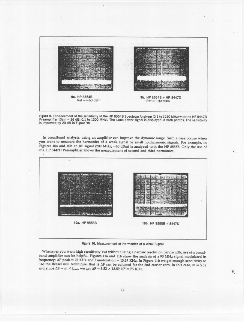
98. HP 85548Ref = -60 dBm

9b. HP 85548 + HP84470Ref = -90 d8m

Figure9. Enhancement of the sensitivity of the HP 85548 Spectrum Analyzer (0.1 to 1250 MHz) with the HP 84470Preamplifier (Gain = 26 dB; 0.1 to 1300 MHz). The same power signal is displayed in both photos. The sensitivityis improved by 20 dB in Figure 9b.

In broadband analysis, using an amplifier can improve the dynamic range. Such a case occurs whenyou want to measure the harmonics of a weak signal or small nonharmonic signals. For example, inFigures lOa and lOb an RF signal (200 MHz; -60 dBm) is analyzed with the HP 8558B. Only the use ofthe HP 8447D Preamplifier allows the measurement of second and third harmonics.

10a.HP 85588

'-.

10b. HP 85588 + 84470

f"lIUre 10. Measurement of Harmonics of a Weak Signal

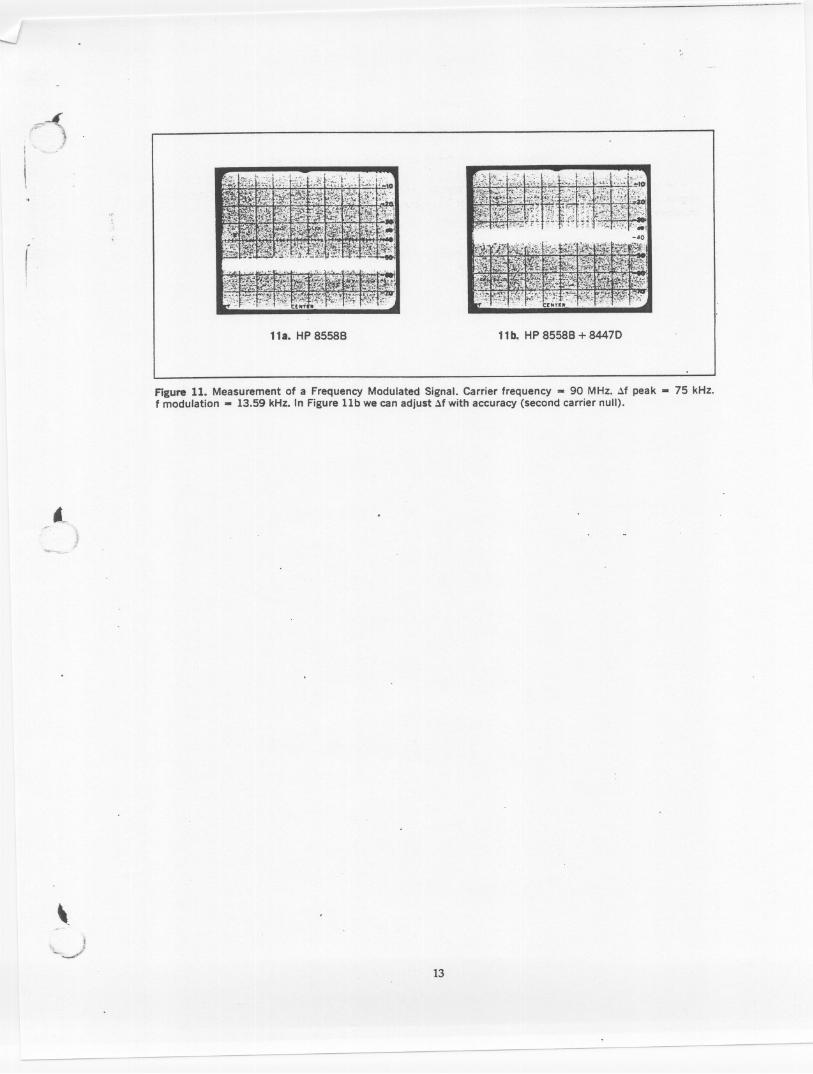
Whenever you want high sensitivity but without using a narrow resolution bandwidth, use of a broad-band amplifier can be helpful. Figures 11a and 11b show the analysis of a 90 MHz signal modulated infrequency; .:IF peak = 75 KHz and f modulation = 13.59 KHz. In Figure 11b we get enough sensitivity touse the Bessel' null technique, that is .:IFcan be adjusted for the 2nd carrier zero. In this case, m = 5.52and since .:IF = m x fmod'we get .1F = 5.52 x 13.59 1Q3= 75 KHz.

t

12

J-..,

-.~p '\

I .1

\

(

11a. HP 85588 11b. HP 85588 + 8447D

Figure 11. Measurement of a Frequency Modulated Signal. Carrier frequency -90 MHz. ~f peak -75 kHz.f modulation -13.59 kHz. 'n Figure lIb we can adjust ~f with accuracy (second carrier null).

.~

-" J

,-

t"-J

13

CHAPTER 3

Signal Enhancement in AM Measurements

The spectrum analyzer is a very powerful tool for measuring the sidebands of an amplitude modulatedsignal. However, in some cases, it may not have enough resolution,' dynamic range or sensitivity tomeasure:

. the intermodulation products resulting from two closely spaced tones. the ripple from the power line. the modulation of weak signals in radio navigation application (localizer and glideslope) .

In this chapter we will explain a method which improves the spectrum analyzer's capability of analyzingsuch amplitude modulated signals.

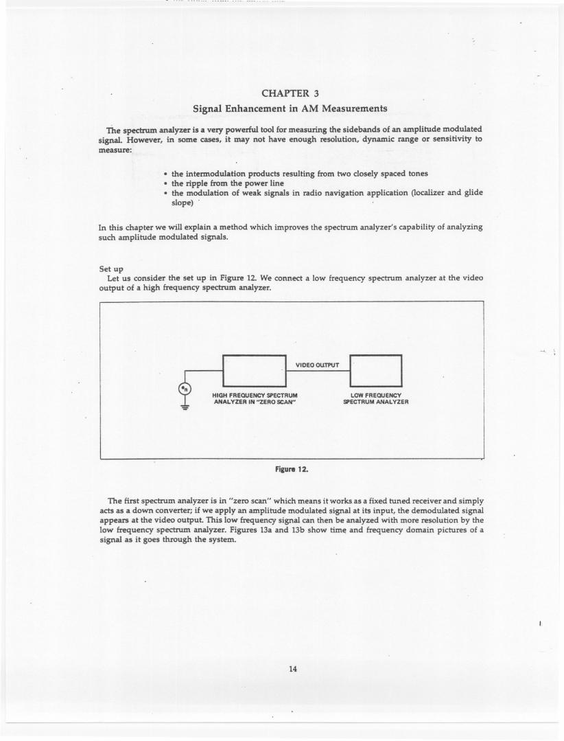
Set upLet us consider the set up in Figure 12. We connect a low frequency spectrum analyzer at the video

output of a high frequency spectrum analyzer.

-~

VIDEO OUTPUT

HIGH FREQUENCY SPECTRUMANALYZER IN "ZERO SCAN"

LOW FREQUENCYSPECTRUM ANALYZER....

Filllre 12.

The first spectrum analyzer is in "zero scan" which means it works as a fixed tuned receiver and simplyacts as a down converter; if we apply an amplitude modulated signal at its input, the demodulated signalappears at the video output. This low frequency signal can then be analyzed with more resolution by thelow frequency spectrum analyzer. Figures 13a and 13b show time and frequency domain pictures of asignal as it goes through the system.

I

14

?~

'~- )A A

(11 TIME DOMAIN 121 TIME DOMAIN

f MODULATION

LOW FPEQUENCY SA', DISPLAVFREQUENCV DOMAIN

(WORKING A!S A RECEIVERI

Figure 13a.

A A

~-".- ..,f,1~~..' 1,1'.1

1WLfc f

SPECTRAL COMPONENTS OF THE INPUT SIGNAL

kmE""2

kE'

a fMOD 2fMOD

SPECTRAL COMPONENTS ON THE SCREEN OFTHE LOW FREQUENCY SPECTRUM ANAL VZER

Figure 13b.

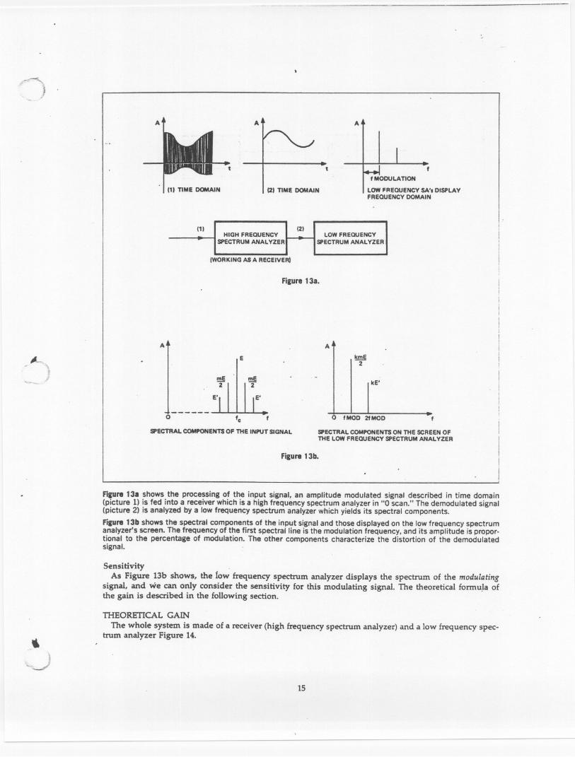
FilUre 13a shows the processing of the input signal, an amplitude modulated signal described in time domain(picture 1) is fed into a receiver which is a high frequency spectrum analyzer in "0 scan." The demodulated signal(picture 2) is analyzed by a low frequency spectrum analyzer which yields its spectral components.

FilUre 13b shows the spectral components of the input signal and those displayed on the low frequency spectrumanalyzer's screen. The frequency of the first spectral line is the modulation frequency, and its amplitude is propor-tional to the percentage of modulation. The other components characterize the distortion of the demodulatedsignal. .

Sensitivity .As Figure 13b shows, the iow frequency spectrum analyzer displays the spectrum of the modulating

signal, and we can only consider the sensitivity for this modulating signal. The theoretical formula ofthe gain is described in the following section.

,1

-~J

THEORETICAL GAIN

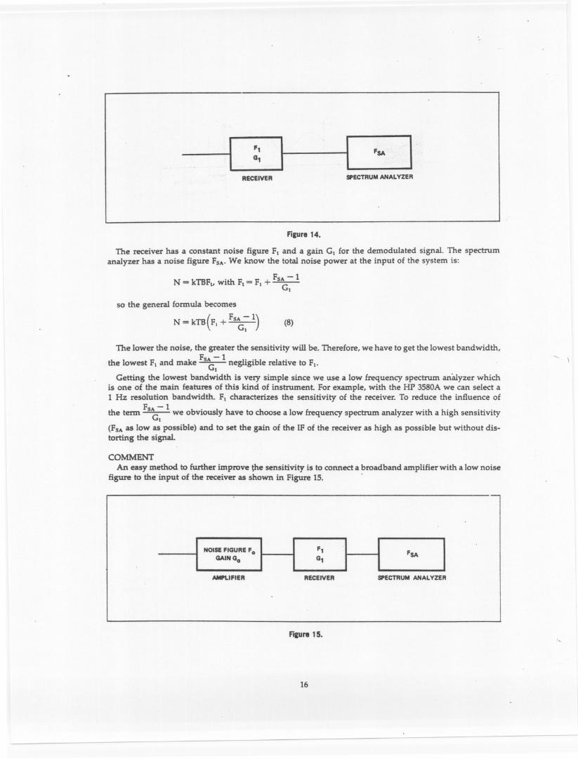
The whole system is made of a receiver (high frequency spectrum analyzer) and a low frequency spec-trum analyzer Figure 14.

15

(1J (21HIGH FREQUENCV LOW FREDUENCV

SPECTRUM ANAL VZER SPECTRUM ANAL VZER

I

F,0,

IFSA

IRECEIVER SPECTRUM ANALYZER

FilUre 14.

The receiver has a constant noise figure F. and a gain G. for the demodulated signal. The spectrumanalyzer has a noise figure FSA.We know the total noise power at the input of the system is:

. FSA- 1N = kTBF.,Wlth FI= F. +--c;-

so the general formula becomes

N = kTB( FI + Fs~~ 1) (8)

The lower the noise, the greater the sensitivity will be. Therefore, we have to get the lowest bandwidth,

the lowest F. and make Fs~~ 1 negligible relative to F..Getting the lowest bandwidth is very simple since we use a low frequency spectrum anaJyzer which

is one of the main features of this kind of instrument For example, with the HP 3580A we can select a1 Hz resolution bandwidth. F. characterizes the sensitivity of the receiver. To reduce the influence of

the term Fs~~ 1 we obviously have to choose a low frequency spectrum analyzer with a high sensitivity(FSAas low as possible) and to set the gain of the IF of the receiver as high as possible but without dis-torting the signal

~ \

COMMENT

An easy method to further improve the sensitivity is to connect a broadband amplifier with a low noisefigure to the input of the receiver as shown in Figure 15. .

NOISE FIGURE Fo

GAIN Go

AMPLIFIER

F,0, H FSA

RECEIVER SPECTRUM ANALYZER

f"'lIUre 15. '.

16

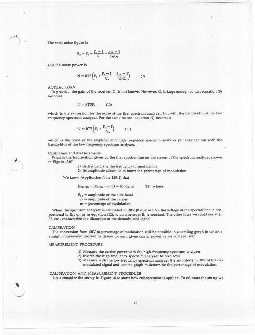
~} The total noise figure is

F - 1 FSA- 11+-FT=Fo+ --cr.- GIGO

and the noise power is

(F - 1 FSI.- 1)1+-

N =kTB Fo+ --c:- GIGO(9)

AcruALGAINIn practice, the gain of the receiver, GI is not known. However, GI is large enough so that equation (8)

becomes

N = kTBF, . (10)

which is the expression for the noise of the first spectrum analyzer, but with the bandwidth of the lowfrequency spectrum analyzer. For the same reason, equation (9) becomes:

N ... kTB(Fo+ \;: 1) (11)

which is the noise of the amplifier and high frequency spectrum analyzer put together but with thebandwidth of the low frequency spectrum analyzer.

. _tL

Calibration and Measurements .

What is the information given by the first spectral line on the screen of the spectrum analyzer shownin Figure 13b?'. .

. 1) itslrequency is the frequency of modulation2) its amplitude allows us to know the percentage of modulation

We know (Application Note 150-1) that

(EsB)dB- (Ec)dB+ 6 dB = 20 log m (12), where

ESB= amplitude of the side bandEc= amplitude of the carrierm = percentage of modulation

When the spectrum analyzer is calibrated in. dBV (0 dBV = 1 V), the voltage of the spectral line is pro-portional to ESBor, as in equation (12), to m, whenever Ec is constant. The other lines we could see at 2f,3f, etc., characterize the distortion of the demodulated signal.

CALIBRATIONThe conversion from dBV to percentage of modulation will be possible in a semiIog graph in which a

straight conversion line will be drawn for each given carrier power as we will see later.

MEASUREMENT PROCEDURE

1) Measure the carrier power with the high frequency spectrum analyzer.2) Switch the high frequency spectrum analyzer to zero scan.3) Measure with the low frequency spectrum analyzer the amplitude in dBV of the de-

modulated signal and use the graph to determine the percentage of modulation.

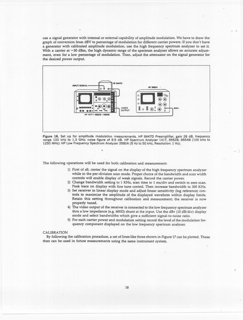
CALIBRATION AND MEASUREMENT PROCEDURELet's consider the set up ill Figure 16 to show how enhancement is applied. To calibrate the set up we

,t

~c-...J

17

"-- ..\

use a signal generator with internal or external capability of amplitude modulation. We have to draw thegraph of conversion from dBV to percentage of modulation for different carrier powers; If you don't havea generator with calibrated amplitude modulation, use the high frequency spectrum analyzer to set it.With a carrier at -30 dBm, the high dynamic range of the spectrum analyzer allows an accurate adjust-ment, even for a low percentage of modulation. Then, adjust the attenuator on the signal generator forthe desired power output.

:D: .@@@.. ... : :

HP ,.,T +85628+-

HP_70INPUT SIGNAl.

HP 3&8OA '

o D .~0 @@0 @@. :,-,,8"8' G: 0 . \!.I.~ 0

VIDEOOUTPUT

soon

Figure 16. Set ,up for amplitude modulation measurements. HP 8447D Preamplifier, gain 26 dB. frequencyrange 100 kHz to 1.3 GHz; noise figure of 8.5 dB. HP Spectrum Analyzer 141T, 8552B. 8554B (100 kHz to1250 MHz) HP Low Frequency Spectrum Analyzer 3580A (5 Hz to 50 kHz, Resolution: 1 Hz).

'~< :

The following operations will be used for both calibration and measurement:

1) First of all, center the signal on the display of the high frequency spectrum analyzerwhile in the per-division scan mode. Proper choice of the bandwidth and scan widthcontrols will enable display of weak signals. Record the carrier power.

2) Change bandwidth setting to 1 KHz, scan time to 1 ms/div and switch to zero scan.Peak trace on display with fine tune control. Then increase bandwidth to 300 KHz.

3) Set receiver in linear display mode and adjust linear sensitivity (log reference) con-trols to maximize the amplitude of the displayed waveform within display limits.Retain this setting throughout calibration and measurement; the receiver is nowproperly tuned.

4) The video output of the receiver is connected to the low frequency spectrum analyzerthru a low impedance (e.g. 6000) shunt at the input. Use the dBv (10 dB/div) displaymode and select bandwidths which give a sufficient signal-to-noise ratio.

5) For each carrier power and modulation setting record the level of the modulation fre-quency component displayed on the low frequency spectrum analyzer.

CALIBRATION.

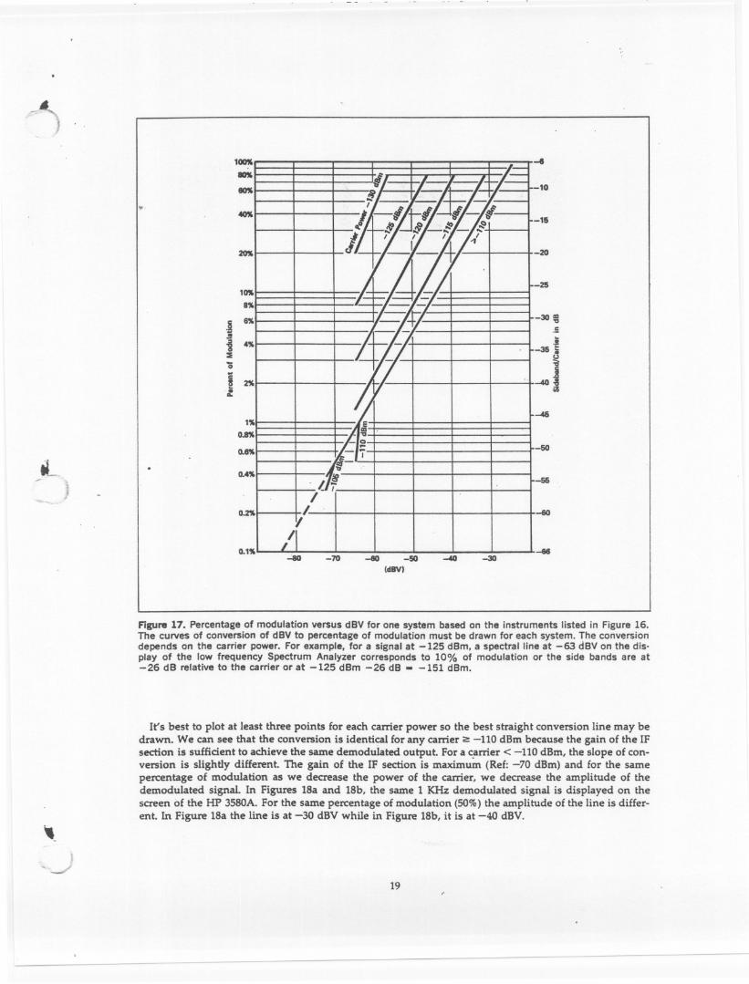
By following the calibration procedure, a set of lines like those shown in Figure 17 can be plotted. Thesethen can be used in future measurements using the same instrument system.

18

~~

1~

8%

--1OK~~ 10

..4K

15

~ 20

,25

.j 8%

i 4"~

30'8.5

'0

~.'c

=1i Z"'....--

1"0.8%

0.8% 50

11- 0.4"-65

-, Jo.Z" -60

0.1"-60 -70 -80 -50

IclBVl-40 -30

-68

Figure 17. Percentage of modulation versus dBYfor one system based on the instruments listed in Figure 16.The curves of conversion of dBY to percentage of modulation must be drawn for each system. The conversiondepends on the carrier power. For example, for a signal at -125 dBm, a spectral line at -63 dBYon the dis.play of the low frequency Spectrum Analyzer corresponds to 10% of modulation or the side bands are at-26 dB relative to the carrier or at -125 dBm -26 dB - -151 dBm.

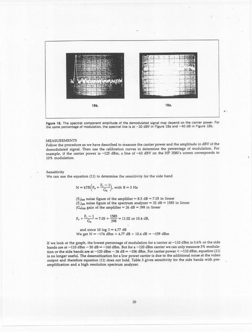
It's best to plot at least three points for each carrier power so the best straight conversion line may bedrawn. We can see that the conversion is identical for any carrier:!: -110 dBm because the gain of the IFsection is sufficient to achieve the same demodulated output. For a c.arrier < -110 dBm, the slope of con-version is slightly different. The gain of the IF section is maximum (Ref: -70 dBm) and for the samepercentage of modulation as we decrease the power of the carrier, we decrease the amplitude of thedemodulated signal. In Figures 18a and 18b, the same 1 KHz demodulated signal is displayed on thescreen of the HP 3580A. For the same percentage of modulation (50%) the amplitude of the line is differ-ent. In Figure 18a the line is at -30 dBY while in Figure 18b, it is at -40 dBY.

'-

, if

19

T/'- 1 '- 1 1'I 1 J 1 -,

If r, I ,

-Iltl/-jf-i -; D-.!'- ..

-I I I I

I "

. /1; .

zWl-

II

1;!7

,-, ...

7 S!L. .Ii

, -J.g "

. iI, I

, /.'y

1'1

18b. 18a.

i.

Figure 18. The spectral component amplitude of tlie demodulated signal may depend on the carrier power. Forthe same percentage of modulation, the spectral line is at -30 dBV in Figure 18a and -40 dB in Figure 18b.

MEASUREMENTSFollow the procedure as we have described to measure the carrier power and the amp~itude in dBV of thedemodulated signal. Then use the calibration curves to determine the percentage of modulation. Forexample, if the carrier power is -125 dBm, a line of -63 dBV on the HP 3580's screen corresponds to10% modulation. \

SensitivityWe can use the equation (11) to determine the sensitivity for the side band

(F -1

)N = kTB Fo+ T ' with B = 3 Hz

(FO)dBnoise figure of the amplifier = 8.5 dB = 7.05 in linear(F.)dBnoise figure of the spectrum analyzer = 32 dB = 1585 in linear(GO)dBgain of the amplifier = 26 dB = 398 in linear

F. - 1 1585Fo+ c;;-= 7.05+ 398 = 11.02or lOAdB,

and since 10 log 3 = 4.77 dBWe get N = -174 dBm + 4.77 dB + lOA dB = -159 dBm

If we look at the graph, the lowest percentage of modulation for a carrier at -110 dBm is 0.6% or the sidebands are at -110 dBm- 50 dB=-160 dBm. But for a -120 dBm carrier we can only measure 3% modula-tion or the side bands are at -120 dBm -36 dB =-156 dBm. For carrier power < -110 dBm, equation (11)is no longer useful. The desensitization for a low power carrier is due to the additional noise at the videooutput and therefore equation (11) does not hold. Table 3 gives sensitivity for the side bands with pre-amplification and a high resolution spectrum analyzer.

20

l.

'

.

~

.

;~'. J

>,.>"

Table 3. Sensitivity for the side bands (amplitude modulation)

COMMENTWithout the preamplifier we will obtain in first approximation the same curve Figure 17 but with a shiftto account for the different carrier power to be measured at the receiver:

At -130 dBm we will substitute -130 dBm + 26 dB = -104 dBm~ -110 dBm becomes ~ -84 dBm.

ApplicationsThe main features are

. high sensitivity for the side bands. high resolution-bandwidth as low as 1 Hz (HP 3580A). frequency range is the low spectrum analyzer's frequency range

~..;.,"r . )~"j'

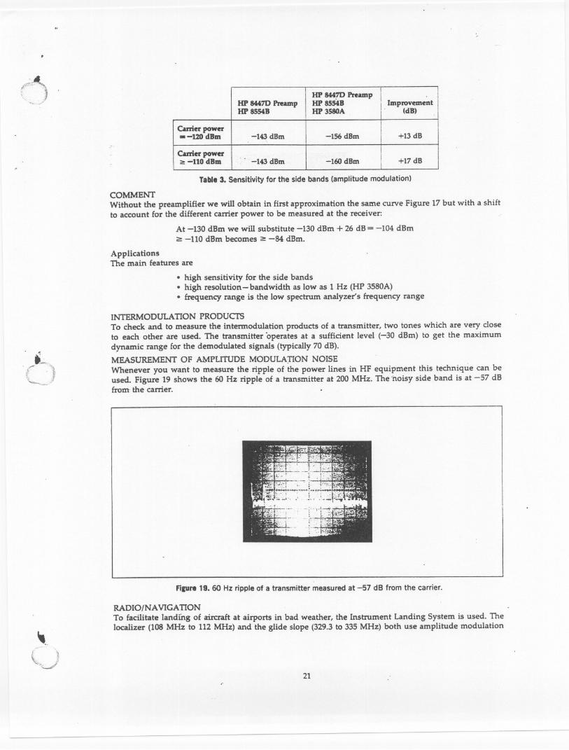
INTERMODULATION PRODUCTSTo check and to measure the intermodulation products of a transmitter, two tones which are very closeto each other are used. The transmitter 'operates at a sufficient level (-30 dBm) to get the maximumdynamic range for the demodulated signals (typically 70 dB).MEASUREMENT OF AMPLITUDE MODULA:TION NOISEWhenever you want to measure the ripple of the power lines in HF equipment this technique can beused. Figure 19 shows the 60 Hz ripple of a transmitter at 200 MHz. The noisy side band is at -57 dBfrom the carrier.

Fipre 19.60 Hz ripple of a transmitter measured at -57 dB from the carrier.

~-i )~.J

RADIO/NA VIGATIONTo facilitate landing of aircraft at airports in bad weather, the Instrument Landing System is used. Thelocalizer (108 MHz to 112 MHz) and the glide slope (329.3 to 335 MHz) both use amplitude modulation

21

HP 84470 Preamp HP 84470 Preamp I . IHP 8554B I ImprovementHP 8554B HP 3S80A i (dB) .

c.rrier power!

- -120 dBm -143 dBm -156 dBm I +13 dB

c.rrier power "

-110 dBm -143 dBm -160 dBm +17 dB

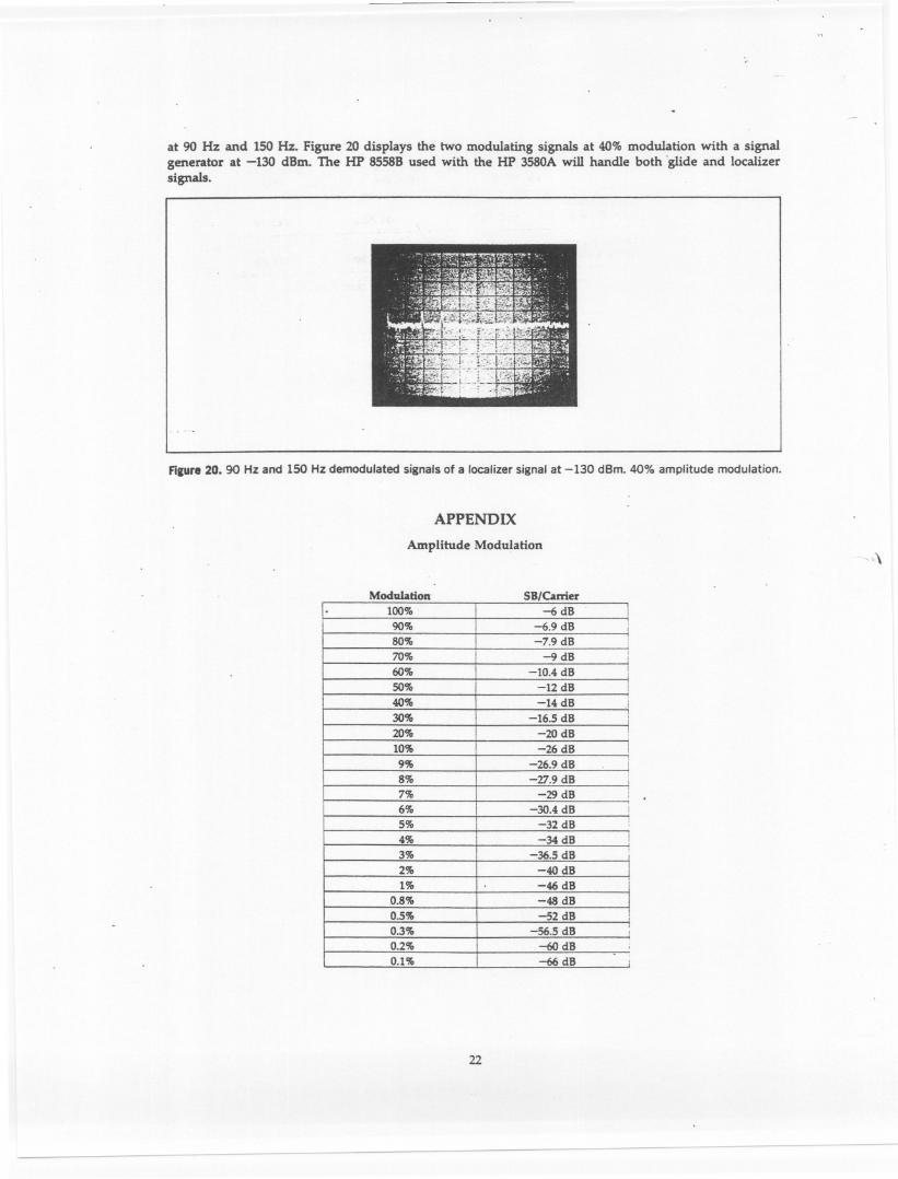
at 90 Hz and 150 Hz. Figure 20 displays the two modulating signals at 40% modulation with a signalgenerator at -130 dBm. The HP 85S8B used with the HP 3580A will handle both 'glide and localizersignals.

filUra 20. 90 Hz and 150 Hz demodulated signals of a localizer signal at -130 dBm. 40% amplitude modulation.

APPENDIX

Amplitude Modulation-..\

Modulation SB/Calrier

22

lOO% -6 dB ,90% -6.9 dB80% -7.9 dB !

70% -9dB :60% -10.4 dB !50% -12 dB40% -14 dB .:30% -16.5 dB '

20% -20 dB !

10% -26 dB9% -26.9 dB8% -27.9 dB7% -29 dB !6% -30.4 dB I

5% -32 dB4% -34 dB3% -36.5 dB i2% -40 dB1% -46 dB i

0.8% -48 dB0.5% -52 dB !0.3% -56.5 dB ,0.2% -60 dB0.1% -66 dB