Embed Size (px)
Citation preview

hp 49g+/ hp 48gII graphing calculator advanced user's reference manual
H Edition 1.1 HP part number F2228-90010
Printed Date: 2006/3/20

Notice REGISTER YOUR PRODUCT AT: www.register.hp.com THIS MANUAL AND ANY EXAMPLES CONTAINED HEREIN ARE PROVIDED "AS IS" AND ARE SUBJECT TO CHANGE WITHOUT NOTICE. HEWLETT-PACKARD COMPANY MAKES NO WARRANTY OF ANY KIND WITH REGARD TO THIS MANUAL, INCLUDING, BUT NOT LIMITED TO, THE IMPLIED WARRANTIES OF MERCHANTABILITY, NON-INFRINGEMENT AND FITNESS FOR A PARTICULAR PURPOSE. HEWLETT-PACKARD CO. SHALL NOT BE LIABLE FOR ANY ERRORS OR FOR INCIDENTAL OR CONSEQUENTIAL DAMAGES IN CONNECTION WITH THE FURNISHING, PERFORMANCE, OR USE OF THIS MANUAL OR THE EXAMPLES CONTAINED HEREIN. © Copyright 1993-1998, 2005, 2006 Hewlett-Packard Development Company, L.P. Reproduction, adaptation, or translation of this manual is prohibited without prior written permission of Hewlett-Packard Company, except as allowed under the copyright laws. Hewlett-Packard Company 4995 Murphy Canyon Rd, Suite 301 San Diego, CA 92123 Acknowledgements Hewlett-Packard would like to thank the following for their contribution: Gene Wright, Tony Hutchins, Wlodek Mier-Jedrzejowicz, Jordi Hidalgo, Ted Kerber, Joe Horn, Richard Nelson, Bruce Horrocks and Jake Schwartz. Printing History Edition 1 September 2005Edition 1.1 March 2006

Contents -1
Contents Contents........................................................................................................................................................................................ 1 1. RPL Programming.................................................................................................................................................................1-1
Understanding Programming .............................................................................................................................................1-1 The Contents of a Program .........................................................................................................................................1-1 Calculations in a Program ...........................................................................................................................................1-2
Entering and Executing Programs......................................................................................................................................1-3 Viewing and Editing Programs ..........................................................................................................................................1-6 Creating Programs on a Computer .....................................................................................................................................1-7 Using Local Variables........................................................................................................................................................1-7
Creating Local Variables.............................................................................................................................................1-7 Evaluating Local Names .............................................................................................................................................1-8 Defining the Scope of Local Variables .......................................................................................................................1-9 Compiled Local Variables.........................................................................................................................................1-10 Creating User-Defined Functions as Programs.........................................................................................................1-10
Using Tests and Conditional Structures ...........................................................................................................................1-11 Testing Conditions ....................................................................................................................................................1-11 Using Conditional Structures and Commands ..........................................................................................................1-13
Using Loop Structures......................................................................................................................................................1-17 Using Definite Loop Structures ................................................................................................................................1-17 Using Indefinite Loop Structures ..............................................................................................................................1-21 Using Loop Counters ................................................................................................................................................1-24 Using Summations Instead of Loops ........................................................................................................................1-25
Using Flags.......................................................................................................................................................................1-25 Types of Flags...........................................................................................................................................................1-26 Setting, Clearing, and Testing Flags .........................................................................................................................1-26 Recalling and Storing the Flag States .......................................................................................................................1-27
Using Subroutines ............................................................................................................................................................1-28 Single-Stepping through a Program .................................................................................................................................1-29 Trapping Errors ................................................................................................................................................................1-32
Causing and Analyzing Errors ..................................................................................................................................1-32 Making an Error Trap ...............................................................................................................................................1-33
Input .................................................................................................................................................................................1-35 Data Input Commands...............................................................................................................................................1-35 Using PROMPT CONT for Input ........................................................................................................................1-35 Using DISP FREEZE HALT CONT for Input ....................................................................................................1-37 Using INPUT ENTER for Input ..........................................................................................................................1-38 Using INFORM and CHOOSE for Input..................................................................................................................1-42 Beeping to Get Attention ..........................................................................................................................................1-45
Stopping a Program for Keystroke Input .........................................................................................................................1-46 Using WAIT for Keystroke Input .............................................................................................................................1-46 Using KEY for Keystroke Input ...............................................................................................................................1-46 Output .......................................................................................................................................................................1-46 Data Output Commands............................................................................................................................................1-47 Labeling Output with Tags .......................................................................................................................................1-47 Labeling and Displaying Output as Strings ..............................................................................................................1-48 Pausing to Display Output ........................................................................................................................................1-48 Using MSGBOX to Display Output .........................................................................................................................1-49
Using Menus with Programs ............................................................................................................................................1-49 Using Menus for Input ..............................................................................................................................................1-50 Using Menus to Run Programs .................................................................................................................................1-50
Turning Off the hp49g+/hp48gII from a Program ...........................................................................................................1-52 2. RPL Programming Examples ................................................................................................................................................2-1
Fibonacci Numbers ............................................................................................................................................................2-1
Contents - 2
FIB1 (Fibonacci Numbers, Recursive Version).......................................................................................................... 2-1 FIB2 (Fibonacci Numbers, Loop Version) ................................................................................................................. 2-2 FIBT (Comparing Program-Execution Time)............................................................................................................. 2-3
Displaying a Binary Integer ............................................................................................................................................... 2-5 PAD (Pad with Leading Spaces) ................................................................................................................................ 2-5 PRESERVE (Save and Restore Previous Status) ....................................................................................................... 2-6 BDISP (Binary Display) ............................................................................................................................................. 2-7
Median of Statistics Data ................................................................................................................................................. 2-10 %TILE (Percentile of a list)...................................................................................................................................... 2-10 MEDIAN (Median of Statistics Data) ...................................................................................................................... 2-11
Expanding and Collecting Completely ............................................................................................................................ 2-14 MULTI (Multiple Execution) ................................................................................................................................... 2-14 EXCO (Expand and Collect Completely)................................................................................................................. 2-15
Minimum and Maximum Array Elements ....................................................................................................................... 2-16 MNX (Minimum or Maximum ElementVersion 1).............................................................................................. 2-16 MNX2 (Minimum or Maximum Element- Version 2).............................................................................................. 2-18
Applying a Program to an Array...................................................................................................................................... 2-20 Converting Between Number Bases ................................................................................................................................ 2-22 Verifying Program Arguments ........................................................................................................................................ 2-24
NAMES (Check List for Exactly Two Names) ........................................................................................................ 2-24 Converting Procedures from Algebraic to RPN .............................................................................................................. 2-27 Bessel Functions .............................................................................................................................................................. 2-29 Animation of Successive Taylor's Polynomials ............................................................................................................... 2-30
SINTP (Converting a Plot to a Graphics Object)...................................................................................................... 2-31 Techniques used in SINTP ....................................................................................................................................... 2-31 SETTS (Superimposing Taylor's polynomials) ........................................................................................................ 2-32 TSA (Animating Taylor's Polynomials) ................................................................................................................... 2-33
Programmatic Use of Statistics and Plotting.................................................................................................................... 2-34 Trace Mode ...................................................................................................................................................................... 2-37 Inverse-Function Solver................................................................................................................................................... 2-38 Animating a Graphical Image .......................................................................................................................................... 2-39
3. Full Command and Function Reference................................................................................................................................ 3-1 ABCUV.............................................................................................................................................................................. 3-4 ABS ................................................................................................................................................................................... 3-4 ACK ................................................................................................................................................................................... 3-4 ACKALL ............................................................................................................................................................................ 3-4 ACOS ................................................................................................................................................................................ 3-5 ACOS2S ........................................................................................................................................................................... 3-6 ACOSH ............................................................................................................................................................................. 3-6 ADD ................................................................................................................................................................................... 3-7 ADDTMOD ....................................................................................................................................................................... 3-8 ADDTOREAL ................................................................................................................................................................... 3-8 ALGB................................................................................................................................................................................. 3-8 ALOG ................................................................................................................................................................................ 3-8 AMORT ............................................................................................................................................................................. 3-8 AND ................................................................................................................................................................................... 3-8 ANIMATE.......................................................................................................................................................................... 3-9 ANS ................................................................................................................................................................................. 3-10 APPLY............................................................................................................................................................................. 3-10 ARC ................................................................................................................................................................................. 3-10 ARCHIVE........................................................................................................................................................................ 3-11 ARG................................................................................................................................................................................. 3-11 ARIT ................................................................................................................................................................................ 3-12 ARRY→ .......................................................................................................................................................................... 3-12 →ARRY .......................................................................................................................................................................... 3-12 ASIN ................................................................................................................................................................................ 3-12 ASIN2C ........................................................................................................................................................................... 3-14 ASIN2T ........................................................................................................................................................................... 3-14
Contents - 3
ASINH..............................................................................................................................................................................3-14 ASN .................................................................................................................................................................................3-14 ASR .................................................................................................................................................................................3-15 ASSUME .........................................................................................................................................................................3-16 ATAN ...............................................................................................................................................................................3-16 ATAN2S ..........................................................................................................................................................................3-17 ATANH ............................................................................................................................................................................3-17 ATICK ..............................................................................................................................................................................3-18 ATTACH..........................................................................................................................................................................3-18 AUGMENT......................................................................................................................................................................3-19 AUTO...............................................................................................................................................................................3-19 AXES ...............................................................................................................................................................................3-20 AXL ..................................................................................................................................................................................3-20 AXM .................................................................................................................................................................................3-20 AXQ .................................................................................................................................................................................3-20 BAR .................................................................................................................................................................................3-20 BARPLOT .......................................................................................................................................................................3-21 BASIS ..............................................................................................................................................................................3-22 BAUD...............................................................................................................................................................................3-22 BEEP ...............................................................................................................................................................................3-22 BESTFIT .........................................................................................................................................................................3-22 BIN ...................................................................................................................................................................................3-22 BINS ................................................................................................................................................................................3-23 BLANK.............................................................................................................................................................................3-23 BOX .................................................................................................................................................................................3-23 BUFLEN ..........................................................................................................................................................................3-24 BYTES.............................................................................................................................................................................3-24 B→R ................................................................................................................................................................................3-24 C2P ..................................................................................................................................................................................3-24 CASCFG .........................................................................................................................................................................3-25 CASCMD ........................................................................................................................................................................3-25 CASE ...............................................................................................................................................................................3-25 CEIL .................................................................................................................................................................................3-25 CENTR ............................................................................................................................................................................3-26 CF ....................................................................................................................................................................................3-26 %CH ................................................................................................................................................................................3-26 CHINREM .......................................................................................................................................................................3-27 CHOLESKY ....................................................................................................................................................................3-27 CHOOSE ........................................................................................................................................................................3-27 CHR .................................................................................................................................................................................3-27 CIRC ................................................................................................................................................................................3-28 CKSM ..............................................................................................................................................................................3-28 CLEAR ............................................................................................................................................................................3-28 CLKADJ ..........................................................................................................................................................................3-28 CLLCD.............................................................................................................................................................................3-29 CLOSEIO ........................................................................................................................................................................3-29 CLΣ ..................................................................................................................................................................................3-29 CLVAR ............................................................................................................................................................................3-29 CMPLX ............................................................................................................................................................................3-29 CNRM..............................................................................................................................................................................3-30 →COL..............................................................................................................................................................................3-30 COL→..............................................................................................................................................................................3-30 COL ...............................................................................................................................................................................3-30 COL+ ...............................................................................................................................................................................3-31 COLCT ............................................................................................................................................................................3-31 COLLECT .......................................................................................................................................................................3-31 COLΣ ...............................................................................................................................................................................3-31 COMB..............................................................................................................................................................................3-32
Contents - 4
CON................................................................................................................................................................................. 3-32 COND.............................................................................................................................................................................. 3-33 CONIC............................................................................................................................................................................. 3-33 CONJ............................................................................................................................................................................... 3-34 CONLIB........................................................................................................................................................................... 3-34 CONST ........................................................................................................................................................................... 3-35 CONSTANTS ................................................................................................................................................................. 3-35 CONT .............................................................................................................................................................................. 3-35 CONVERT ...................................................................................................................................................................... 3-35 CORR.............................................................................................................................................................................. 3-35 COS................................................................................................................................................................................. 3-36 COSH .............................................................................................................................................................................. 3-36 COV................................................................................................................................................................................. 3-37 CR.................................................................................................................................................................................... 3-37 CRDIR............................................................................................................................................................................. 3-37 CROSS ........................................................................................................................................................................... 3-37 CSWP ............................................................................................................................................................................. 3-38 CURL............................................................................................................................................................................... 3-38 CYCLOTOMIC ............................................................................................................................................................... 3-38 CYLIN.............................................................................................................................................................................. 3-38 C→PX ............................................................................................................................................................................. 3-38 C→R................................................................................................................................................................................ 3-39 DARCY ........................................................................................................................................................................... 3-39 DATE............................................................................................................................................................................... 3-39 →DATE ........................................................................................................................................................................... 3-39 DATE+ ............................................................................................................................................................................ 3-40 DBUG .............................................................................................................................................................................. 3-40 DDAYS............................................................................................................................................................................ 3-40 DEC ................................................................................................................................................................................. 3-41 DECR .............................................................................................................................................................................. 3-41 DEDICACE..................................................................................................................................................................... 3-41 DEF ................................................................................................................................................................................. 3-41 DEFINE........................................................................................................................................................................... 3-41 DEG................................................................................................................................................................................. 3-42 DEGREE......................................................................................................................................................................... 3-42 DELALARM .................................................................................................................................................................... 3-42 DELAY ............................................................................................................................................................................ 3-42 DELKEYS ....................................................................................................................................................................... 3-42 DEPND ........................................................................................................................................................................... 3-43 DEPTH ............................................................................................................................................................................ 3-44 DERIV ............................................................................................................................................................................. 3-44 DERVX............................................................................................................................................................................ 3-44 DESOLVE....................................................................................................................................................................... 3-44 DET ................................................................................................................................................................................. 3-44 DETACH ......................................................................................................................................................................... 3-44 DIAG→............................................................................................................................................................................ 3-45 →DIAG............................................................................................................................................................................ 3-45 DIAGMAP ....................................................................................................................................................................... 3-45 DIFF................................................................................................................................................................................. 3-45 DIFFEQ........................................................................................................................................................................... 3-46 DIR................................................................................................................................................................................... 3-47 DISP ................................................................................................................................................................................ 3-47 DISPXY ........................................................................................................................................................................... 3-47 DISTRIB.......................................................................................................................................................................... 3-48 DIV................................................................................................................................................................................... 3-48 DIV2................................................................................................................................................................................. 3-48 DIV2MOD ....................................................................................................................................................................... 3-48 DIVIS ............................................................................................................................................................................... 3-48
Contents - 5
DIVMOD..........................................................................................................................................................................3-48 DIVPC..............................................................................................................................................................................3-48 dn .....................................................................................................................................................................................3-48 DO....................................................................................................................................................................................3-48 DOERR ...........................................................................................................................................................................3-49 DOLIST ...........................................................................................................................................................................3-49 DOMAIN..........................................................................................................................................................................3-50 DOSUBS .........................................................................................................................................................................3-50 DOT .................................................................................................................................................................................3-50 DRAW .............................................................................................................................................................................3-51 DRAW3DMATRIX .........................................................................................................................................................3-51 DRAX...............................................................................................................................................................................3-51 DROITE...........................................................................................................................................................................3-52 DROP ..............................................................................................................................................................................3-52 DROP2 ............................................................................................................................................................................3-52 DROPN ...........................................................................................................................................................................3-52 DTAG...............................................................................................................................................................................3-52 DUP .................................................................................................................................................................................3-53 DUP2 ...............................................................................................................................................................................3-53 DUPDUP .........................................................................................................................................................................3-53 DUPN ..............................................................................................................................................................................3-53 D→R ................................................................................................................................................................................3-54 e .......................................................................................................................................................................................3-54 EDIT.................................................................................................................................................................................3-54 EDITB ..............................................................................................................................................................................3-55 EGCD ..............................................................................................................................................................................3-55 EGV .................................................................................................................................................................................3-55 EGVL ...............................................................................................................................................................................3-55 ELSE................................................................................................................................................................................3-55 END .................................................................................................................................................................................3-56 ENDSUB .........................................................................................................................................................................3-56 ENG .................................................................................................................................................................................3-56 EPSX0 .............................................................................................................................................................................3-56 EQNLIB ...........................................................................................................................................................................3-56 EQW ................................................................................................................................................................................3-57 EQ→ ................................................................................................................................................................................3-57 ERASE ............................................................................................................................................................................3-57 ERR0 ...............................................................................................................................................................................3-57 ERRM ..............................................................................................................................................................................3-57 ERRN ..............................................................................................................................................................................3-58 EULER ............................................................................................................................................................................3-58 EVAL................................................................................................................................................................................3-58 EXLR ...............................................................................................................................................................................3-59 EX&LN.............................................................................................................................................................................3-59 EXP..................................................................................................................................................................................3-59 EXP2HYP .......................................................................................................................................................................3-60 EXP2POW ......................................................................................................................................................................3-60 EXPAN ............................................................................................................................................................................3-60 EXPAND .........................................................................................................................................................................3-60 EXPANDMOD ................................................................................................................................................................3-60 EXPFIT............................................................................................................................................................................3-60 EXPLN.............................................................................................................................................................................3-60 EXPM ..............................................................................................................................................................................3-60 EYEPT.............................................................................................................................................................................3-61 F0λ ...................................................................................................................................................................................3-61 FACT ...............................................................................................................................................................................3-61 FACTOR .........................................................................................................................................................................3-62 FACTORMOD ................................................................................................................................................................3-62
Contents - 6
FACTORS ...................................................................................................................................................................... 3-62 FANNING ....................................................................................................................................................................... 3-62 FAST3D .......................................................................................................................................................................... 3-62 FCOEF ............................................................................................................................................................................ 3-63 FC? .................................................................................................................................................................................. 3-63 FC?C ............................................................................................................................................................................... 3-63 FDISTRIB ....................................................................................................................................................................... 3-64 FFT .................................................................................................................................................................................. 3-64 FILER .............................................................................................................................................................................. 3-64 FINDALARM .................................................................................................................................................................. 3-64 FINISH ............................................................................................................................................................................ 3-65 FIX ................................................................................................................................................................................... 3-65 FLASHEVAL .................................................................................................................................................................. 3-65 FLOOR............................................................................................................................................................................ 3-66 FONT6 ............................................................................................................................................................................ 3-66 FONT7 ............................................................................................................................................................................ 3-66 FONT8 ............................................................................................................................................................................ 3-66 FONT→........................................................................................................................................................................... 3-67 →FONT........................................................................................................................................................................... 3-67 FOR ................................................................................................................................................................................. 3-67 FOURIER ....................................................................................................................................................................... 3-68 FP .................................................................................................................................................................................... 3-68 FREE............................................................................................................................................................................... 3-68 FREEZE.......................................................................................................................................................................... 3-68 FROOTS......................................................................................................................................................................... 3-69 FS? .................................................................................................................................................................................. 3-69 FS?C ............................................................................................................................................................................... 3-69 FUNCTION..................................................................................................................................................................... 3-70 FXND............................................................................................................................................................................... 3-71 GAMMA .......................................................................................................................................................................... 3-71 GAUSS ........................................................................................................................................................................... 3-71 GBASIS........................................................................................................................................................................... 3-71 GCD................................................................................................................................................................................. 3-71 GCDMOD ....................................................................................................................................................................... 3-71 GET ................................................................................................................................................................................. 3-71 GETI ................................................................................................................................................................................ 3-72 GOR ................................................................................................................................................................................ 3-73 GRAD .............................................................................................................................................................................. 3-73 GRAMSCHMIDT ........................................................................................................................................................... 3-73 GREDUCE ..................................................................................................................................................................... 3-73 GRIDMAP ....................................................................................................................................................................... 3-73 →GROB.......................................................................................................................................................................... 3-74 GROB.............................................................................................................................................................................. 3-74 GROBADD ..................................................................................................................................................................... 3-74 GXOR.............................................................................................................................................................................. 3-75 HADAMARD................................................................................................................................................................... 3-75 HALFTAN ....................................................................................................................................................................... 3-75 HALT ............................................................................................................................................................................... 3-75 HEAD .............................................................................................................................................................................. 3-75 HEADER→ ..................................................................................................................................................................... 3-76 →HEADER ..................................................................................................................................................................... 3-76 HELP ............................................................................................................................................................................... 3-76 HERMITE ....................................................................................................................................................................... 3-76 HESS............................................................................................................................................................................... 3-76 HEX ................................................................................................................................................................................. 3-76 HILBERT......................................................................................................................................................................... 3-77 HISTOGRAM ................................................................................................................................................................. 3-77 HISTPLOT ...................................................................................................................................................................... 3-77
Contents - 7
HMS...............................................................................................................................................................................3-78 HMS+ ..............................................................................................................................................................................3-78 HMS→ .............................................................................................................................................................................3-79 →HMS .............................................................................................................................................................................3-79 HOME..............................................................................................................................................................................3-79 HORNER ........................................................................................................................................................................3-79 i.........................................................................................................................................................................................3-80 IABCUV ...........................................................................................................................................................................3-80 IBASIS .............................................................................................................................................................................3-80 IBERNOULLI ..................................................................................................................................................................3-80 IBP ...................................................................................................................................................................................3-80 ICHINREM ......................................................................................................................................................................3-80 IDN...................................................................................................................................................................................3-80 IDIV2................................................................................................................................................................................3-81 IEGCD .............................................................................................................................................................................3-81 IF ......................................................................................................................................................................................3-81 IFERR..............................................................................................................................................................................3-81 IFFT .................................................................................................................................................................................3-82 IFT....................................................................................................................................................................................3-83 IFTE .................................................................................................................................................................................3-83 ILAP .................................................................................................................................................................................3-83 IM .....................................................................................................................................................................................3-83 IMAGE .............................................................................................................................................................................3-84 INCR ................................................................................................................................................................................3-84 INDEP..............................................................................................................................................................................3-84 INFORM ..........................................................................................................................................................................3-85 INPUT..............................................................................................................................................................................3-86 INT ...................................................................................................................................................................................3-86 INTEGER ........................................................................................................................................................................3-87 INTVX ..............................................................................................................................................................................3-87 INV ...................................................................................................................................................................................3-87 INVMOD..........................................................................................................................................................................3-87 IP ......................................................................................................................................................................................3-87 IQUOT .............................................................................................................................................................................3-87 IREMAINDER.................................................................................................................................................................3-87 ISOL.................................................................................................................................................................................3-87 ISOM................................................................................................................................................................................3-88 ISPRIME? .......................................................................................................................................................................3-88 I→R..................................................................................................................................................................................3-88 JORDAN .........................................................................................................................................................................3-88 KER .................................................................................................................................................................................3-88 KERRM ...........................................................................................................................................................................3-88 KEY..................................................................................................................................................................................3-89 KEYEVAL........................................................................................................................................................................3-89 →KEYTIME ....................................................................................................................................................................3-89 KEYTIME→ ....................................................................................................................................................................3-89 KGET ...............................................................................................................................................................................3-90 KILL .................................................................................................................................................................................3-90 LABEL .............................................................................................................................................................................3-90 LAGRANGE....................................................................................................................................................................3-90 LANGUAGE→................................................................................................................................................................3-91 →LANGUAGE................................................................................................................................................................3-91 LAP ..................................................................................................................................................................................3-91 LAPL ................................................................................................................................................................................3-91 LAST................................................................................................................................................................................3-91 LASTARG .......................................................................................................................................................................3-91 LCD→..............................................................................................................................................................................3-92 →LCD..............................................................................................................................................................................3-92
Contents - 8
LCM ................................................................................................................................................................................. 3-92 LCXM .............................................................................................................................................................................. 3-92 LDEC............................................................................................................................................................................... 3-92 LEGENDRE ................................................................................................................................................................... 3-92 LGCD .............................................................................................................................................................................. 3-92 LIBEVAL ......................................................................................................................................................................... 3-92 LIBS................................................................................................................................................................................. 3-93 lim .................................................................................................................................................................................... 3-93 LIMIT ............................................................................................................................................................................... 3-93 LIN ................................................................................................................................................................................... 3-93 LINE................................................................................................................................................................................. 3-93 ΣLINE .............................................................................................................................................................................. 3-93 LINFIT ............................................................................................................................................................................. 3-94 LININ ............................................................................................................................................................................... 3-94 LINSOLVE ...................................................................................................................................................................... 3-94 LIST→ ............................................................................................................................................................................. 3-94 →LIST ............................................................................................................................................................................. 3-94 ∆LIST............................................................................................................................................................................... 3-95 ΠLIST .............................................................................................................................................................................. 3-95 ΣLIST............................................................................................................................................................................... 3-95 LN .................................................................................................................................................................................... 3-95 LNAME............................................................................................................................................................................ 3-96 LNCOLLECT .................................................................................................................................................................. 3-97 LNP1 ............................................................................................................................................................................... 3-97 LOCAL ............................................................................................................................................................................ 3-97 LOG ................................................................................................................................................................................. 3-97 LOGFIT ........................................................................................................................................................................... 3-98 LQ .................................................................................................................................................................................... 3-98 LR .................................................................................................................................................................................... 3-98 LSQ ................................................................................................................................................................................. 3-99 LU .................................................................................................................................................................................... 3-99 LVAR ............................................................................................................................................................................. 3-100 MAD............................................................................................................................................................................... 3-100 MAIN ............................................................................................................................................................................. 3-100 MANT ............................................................................................................................................................................ 3-100 MAP............................................................................................................................................................................... 3-100 ↓MATCH ....................................................................................................................................................................... 3-100 ↑MATCH ....................................................................................................................................................................... 3-101 MATHS ......................................................................................................................................................................... 3-101 MATR ............................................................................................................................................................................ 3-101 MAX............................................................................................................................................................................... 3-101 MAXR ............................................................................................................................................................................ 3-102 MAXΣ ............................................................................................................................................................................ 3-102 MCALC ......................................................................................................................................................................... 3-102 MEAN ............................................................................................................................................................................ 3-103 MEM .............................................................................................................................................................................. 3-103 MENU............................................................................................................................................................................ 3-103 MENUXY ...................................................................................................................................................................... 3-104 MERGE......................................................................................................................................................................... 3-104 MIN ................................................................................................................................................................................ 3-104 MINEHUNT .................................................................................................................................................................. 3-104 MINIFONT→ ................................................................................................................................................................ 3-105 →MINIFONT ................................................................................................................................................................ 3-105 MINIT............................................................................................................................................................................. 3-105 MINR ............................................................................................................................................................................. 3-106 MINΣ.............................................................................................................................................................................. 3-106 MITM ............................................................................................................................................................................. 3-106 MKISOM ....................................................................................................................................................................... 3-106
Contents - 9
MOD ..............................................................................................................................................................................3-106 MODSTO ......................................................................................................................................................................3-107 MODULAR....................................................................................................................................................................3-107 MROOT .........................................................................................................................................................................3-107 MSGBOX ......................................................................................................................................................................3-107 MSLV .............................................................................................................................................................................3-107 MSOLVR .......................................................................................................................................................................3-107 MULTMOD....................................................................................................................................................................3-108 MUSER .........................................................................................................................................................................3-108 →NDISP........................................................................................................................................................................3-108 NDIST............................................................................................................................................................................3-108 NDUPN .........................................................................................................................................................................3-109 NEG ...............................................................................................................................................................................3-109 NEWOB.........................................................................................................................................................................3-109 NEXT .............................................................................................................................................................................3-110 NEXTPRIME ................................................................................................................................................................3-110 NIP .................................................................................................................................................................................3-110 NOT ...............................................................................................................................................................................3-110 NOVAL ..........................................................................................................................................................................3-111 NΣ ..................................................................................................................................................................................3-111 NSUB.............................................................................................................................................................................3-111 →NUM...........................................................................................................................................................................3-111 NUM...............................................................................................................................................................................3-112 NUMX ............................................................................................................................................................................3-112 NUMY ............................................................................................................................................................................3-112 OBJ→ ............................................................................................................................................................................3-113 OCT ...............................................................................................................................................................................3-113 OFF................................................................................................................................................................................3-113 OLDPRT........................................................................................................................................................................3-114 OPENIO ........................................................................................................................................................................3-114 OR..................................................................................................................................................................................3-114 ORDER .........................................................................................................................................................................3-115 OVER ............................................................................................................................................................................3-115 P2C ................................................................................................................................................................................3-115 PA2B2 ...........................................................................................................................................................................3-115 PARAMETRIC..............................................................................................................................................................3-116 PARITY .........................................................................................................................................................................3-116 PARSURFACE ............................................................................................................................................................3-117 PARTFRAC ..................................................................................................................................................................3-118 PATH .............................................................................................................................................................................3-118 PCAR.............................................................................................................................................................................3-118 PCOEF ..........................................................................................................................................................................3-118 PCONTOUR .................................................................................................................................................................3-118 PCOV ............................................................................................................................................................................3-119 PDIM..............................................................................................................................................................................3-119 PERM ............................................................................................................................................................................3-120 PEVAL ...........................................................................................................................................................................3-120 PGDIR ...........................................................................................................................................................................3-120 PICK ..............................................................................................................................................................................3-121 PICK3 ............................................................................................................................................................................3-121 PICT...............................................................................................................................................................................3-121 PICTURE ......................................................................................................................................................................3-121 PINIT..............................................................................................................................................................................3-122 PIX? ...............................................................................................................................................................................3-122 PIXOFF .........................................................................................................................................................................3-122 PIXON ...........................................................................................................................................................................3-122 PKT ................................................................................................................................................................................3-122 PLOT .............................................................................................................................................................................3-123
Contents - 10
PLOTADD..................................................................................................................................................................... 3-123 PMAX ............................................................................................................................................................................ 3-123 PMIN ............................................................................................................................................................................. 3-123 PMINI ............................................................................................................................................................................ 3-124 POLAR .......................................................................................................................................................................... 3-124 POLYNOMIAL.............................................................................................................................................................. 3-125 POP ............................................................................................................................................................................... 3-125 POS ............................................................................................................................................................................... 3-125 POTENTIAL ................................................................................................................................................................. 3-125 POWEXPAND.............................................................................................................................................................. 3-125 POWMOD..................................................................................................................................................................... 3-125 PR1................................................................................................................................................................................ 3-125 PREDV.......................................................................................................................................................................... 3-126 PREDX.......................................................................................................................................................................... 3-126 PREDY.......................................................................................................................................................................... 3-127 PREVAL........................................................................................................................................................................ 3-127 PREVPRIME ................................................................................................................................................................ 3-127 PRLCD .......................................................................................................................................................................... 3-128 PROMPT ...................................................................................................................................................................... 3-128 PROMPTSTO .............................................................................................................................................................. 3-128 PROOT ......................................................................................................................................................................... 3-128 PROPFRAC ................................................................................................................................................................. 3-129 PRST............................................................................................................................................................................. 3-129 PRSTC .......................................................................................................................................................................... 3-129 PRVAR.......................................................................................................................................................................... 3-129 PSDEV .......................................................................................................................................................................... 3-130 PSI ................................................................................................................................................................................. 3-130 Psi .................................................................................................................................................................................. 3-130 PTAYL........................................................................................................................................................................... 3-130 PURGE ......................................................................................................................................................................... 3-131 PUSH ............................................................................................................................................................................ 3-131 PUT ............................................................................................................................................................................... 3-131 PUTI .............................................................................................................................................................................. 3-132 PVAR............................................................................................................................................................................. 3-133 PVARS .......................................................................................................................................................................... 3-133 PVIEW........................................................................................................................................................................... 3-134 PWRFIT ........................................................................................................................................................................ 3-134 PX→C ........................................................................................................................................................................... 3-134 →Q ................................................................................................................................................................................ 3-135 →Qπ .............................................................................................................................................................................. 3-135 qr .................................................................................................................................................................................... 3-135 QR ................................................................................................................................................................................. 3-136 QUAD ............................................................................................................................................................................ 3-136 QUOT ............................................................................................................................................................................ 3-136 QUOTE ......................................................................................................................................................................... 3-136 QXA ............................................................................................................................................................................... 3-137 RAD ............................................................................................................................................................................... 3-137 RAND ............................................................................................................................................................................ 3-137 RANK ............................................................................................................................................................................ 3-137 RANM............................................................................................................................................................................ 3-138 RATIO ........................................................................................................................................................................... 3-138 RCEQ ............................................................................................................................................................................ 3-139 RCI................................................................................................................................................................................. 3-139 RCIJ............................................................................................................................................................................... 3-139 RCL ............................................................................................................................................................................... 3-139 RCLALARM.................................................................................................................................................................. 3-140 RCLF ............................................................................................................................................................................. 3-140 RCLKEYS ..................................................................................................................................................................... 3-141
Contents - 11
RCLMENU ....................................................................................................................................................................3-141 RCLVX ..........................................................................................................................................................................3-141 RCLΣ .............................................................................................................................................................................3-141 RCWS ...........................................................................................................................................................................3-142 RDM...............................................................................................................................................................................3-142 RDZ ...............................................................................................................................................................................3-142 RE ..................................................................................................................................................................................3-143 RECN ............................................................................................................................................................................3-143 RECT .............................................................................................................................................................................3-143 RECV.............................................................................................................................................................................3-144 REF................................................................................................................................................................................3-144 REMAINDER ................................................................................................................................................................3-144 RENAME.......................................................................................................................................................................3-144 REORDER....................................................................................................................................................................3-144 REPEAT........................................................................................................................................................................3-144 REPL .............................................................................................................................................................................3-144 RES ...............................................................................................................................................................................3-145 RESTORE ....................................................................................................................................................................3-146 RESULTANT ................................................................................................................................................................3-146 REVLIST .......................................................................................................................................................................3-146 REWRITE .....................................................................................................................................................................3-147 RISCH ...........................................................................................................................................................................3-147 RKF................................................................................................................................................................................3-147 RKFERR .......................................................................................................................................................................3-147 RKFSTEP .....................................................................................................................................................................3-148 RL...................................................................................................................................................................................3-148 RLB ................................................................................................................................................................................3-148 RND ...............................................................................................................................................................................3-149 RNRM............................................................................................................................................................................3-149 ROLL .............................................................................................................................................................................3-150 ROLLD ..........................................................................................................................................................................3-150 ROMUPLOAD ..............................................................................................................................................................3-150 ROOT ............................................................................................................................................................................3-150 ROT ...............................................................................................................................................................................3-151 ROW............................................................................................................................................................................3-151 ROW+............................................................................................................................................................................3-151 ROW→ ..........................................................................................................................................................................3-151 →ROW ..........................................................................................................................................................................3-152 RPL>..............................................................................................................................................................................3-152 RR ..................................................................................................................................................................................3-152 RRB ...............................................................................................................................................................................3-153 rref..................................................................................................................................................................................3-153 RREF .............................................................................................................................................................................3-153 RREFMOD....................................................................................................................................................................3-153 RRK ...............................................................................................................................................................................3-153 RRKSTEP .....................................................................................................................................................................3-154 RSBERR .......................................................................................................................................................................3-155 RSD ...............................................................................................................................................................................3-155 RSWP............................................................................................................................................................................3-156 RULES ..........................................................................................................................................................................3-156 R→B ..............................................................................................................................................................................3-156 R→C ..............................................................................................................................................................................3-156 R→D ..............................................................................................................................................................................3-157 R→I................................................................................................................................................................................3-157 SAME ............................................................................................................................................................................3-157 SBRK .............................................................................................................................................................................3-157 SCALE...........................................................................................................................................................................3-158 SCALEH........................................................................................................................................................................3-158
Contents - 12
SCALEW....................................................................................................................................................................... 3-158 SCATRPLOT................................................................................................................................................................ 3-158 SCATTER ..................................................................................................................................................................... 3-159 SCHUR ......................................................................................................................................................................... 3-159 SCI................................................................................................................................................................................. 3-160 SCLΣ ............................................................................................................................................................................. 3-160 SCONJ .......................................................................................................................................................................... 3-160 SCROLL ....................................................................................................................................................................... 3-160 SDEV............................................................................................................................................................................. 3-161 SEND ............................................................................................................................................................................ 3-161 SEQ ............................................................................................................................................................................... 3-161 SERIES ......................................................................................................................................................................... 3-162 SERVER ....................................................................................................................................................................... 3-162 SEVAL........................................................................................................................................................................... 3-162 SF .................................................................................................................................................................................. 3-162 SHOW ........................................................................................................................................................................... 3-162 SIDENS......................................................................................................................................................................... 3-163 SIGMA........................................................................................................................................................................... 3-163 SIGMAVX ..................................................................................................................................................................... 3-163 SIGN.............................................................................................................................................................................. 3-163 SIGNTAB ...................................................................................................................................................................... 3-164 SIMP2 ........................................................................................................................................................................... 3-164 SIMPLIFY ..................................................................................................................................................................... 3-164 SIN................................................................................................................................................................................. 3-164 SINCOS ........................................................................................................................................................................ 3-164 SINH .............................................................................................................................................................................. 3-164 SINV .............................................................................................................................................................................. 3-165 SIZE............................................................................................................................................................................... 3-165 SL................................................................................................................................................................................... 3-165 SLB ................................................................................................................................................................................ 3-166 SLOPEFIELD ............................................................................................................................................................... 3-166 SNEG ............................................................................................................................................................................ 3-167 SNRM............................................................................................................................................................................ 3-167 SOLVE .......................................................................................................................................................................... 3-167 SOLVEQN .................................................................................................................................................................... 3-167 SOLVER ....................................................................................................................................................................... 3-168 SOLVEVX ..................................................................................................................................................................... 3-168 SORT ............................................................................................................................................................................ 3-168 SPHERE ....................................................................................................................................................................... 3-168 SQ.................................................................................................................................................................................. 3-168 SR .................................................................................................................................................................................. 3-169 SRAD ............................................................................................................................................................................ 3-169 SRB ............................................................................................................................................................................... 3-169 SRECV.......................................................................................................................................................................... 3-169 SREPL .......................................................................................................................................................................... 3-170 START .......................................................................................................................................................................... 3-170 STD ............................................................................................................................................................................... 3-171 STEP ............................................................................................................................................................................. 3-172 STEQ............................................................................................................................................................................. 3-172 STIME ........................................................................................................................................................................... 3-172 STO ............................................................................................................................................................................... 3-172 STOALARM.................................................................................................................................................................. 3-173 STOF............................................................................................................................................................................. 3-173 STOKEYS..................................................................................................................................................................... 3-174 STORE.......................................................................................................................................................................... 3-174 STOVX .......................................................................................................................................................................... 3-174 STO+ ............................................................................................................................................................................. 3-174 STO ............................................................................................................................................................................. 3-174 STO*.............................................................................................................................................................................. 3-175
Contents - 13
STO/ ..............................................................................................................................................................................3-175 STOΣ .............................................................................................................................................................................3-176 STR→............................................................................................................................................................................3-176 →STR............................................................................................................................................................................3-176 STREAM .......................................................................................................................................................................3-176 STURM..........................................................................................................................................................................3-177 STURMAB ....................................................................................................................................................................3-177 STWS ............................................................................................................................................................................3-177 SUB ...............................................................................................................................................................................3-177 SUBST ..........................................................................................................................................................................3-178 SUBTMOD....................................................................................................................................................................3-178 SVD ...............................................................................................................................................................................3-178 SVL ................................................................................................................................................................................3-178 SWAP ............................................................................................................................................................................3-179 SYSEVAL......................................................................................................................................................................3-179 SYLVESTER ................................................................................................................................................................3-179 SYST2MAT...................................................................................................................................................................3-179 %T..................................................................................................................................................................................3-179 TABVAL ........................................................................................................................................................................3-180 TABVAR........................................................................................................................................................................3-180 →TAG............................................................................................................................................................................3-180 TAIL ...............................................................................................................................................................................3-180 TAN................................................................................................................................................................................3-180 TAN2CS2......................................................................................................................................................................3-181 TAN2SC ........................................................................................................................................................................3-181 TAN2SC2......................................................................................................................................................................3-181 TANH .............................................................................................................................................................................3-181 TAYLOR0......................................................................................................................................................................3-181 TAYLR ...........................................................................................................................................................................3-181 TCHEBYCHEFF ..........................................................................................................................................................3-182 TCOLLECT ...................................................................................................................................................................3-182 TDELTA ........................................................................................................................................................................3-182 TESTS ...........................................................................................................................................................................3-182 TEVAL ...........................................................................................................................................................................3-182 TEXPAND .....................................................................................................................................................................3-183 TEXT..............................................................................................................................................................................3-183 THEN .............................................................................................................................................................................3-183 TICKS ............................................................................................................................................................................3-183 TIME ..............................................................................................................................................................................3-183 →TIME ..........................................................................................................................................................................3-183 TINC ..............................................................................................................................................................................3-184 TLIN ...............................................................................................................................................................................3-184 TLINE ............................................................................................................................................................................3-184 TMENU..........................................................................................................................................................................3-184 TOT................................................................................................................................................................................3-185 TRACE ..........................................................................................................................................................................3-185 TRAN .............................................................................................................................................................................3-185 TRANSIO ......................................................................................................................................................................3-185 TRIG ..............................................................................................................................................................................3-186 TRIGCOS......................................................................................................................................................................3-186 TRIGO ...........................................................................................................................................................................3-186 TRIGSIN........................................................................................................................................................................3-186 TRIGTAN ......................................................................................................................................................................3-186 TRN ...............................................................................................................................................................................3-186 TRNC.............................................................................................................................................................................3-186 TRUNC..........................................................................................................................................................................3-187 TRUTH ..........................................................................................................................................................................3-187 TSIMP............................................................................................................................................................................3-188
Contents - 14
TSTR ............................................................................................................................................................................. 3-188 TVARS .......................................................................................................................................................................... 3-188 TVM ............................................................................................................................................................................... 3-188 TVMBEG....................................................................................................................................................................... 3-189 TVMEND....................................................................................................................................................................... 3-189 TVMROOT ................................................................................................................................................................... 3-189 TYPE ............................................................................................................................................................................. 3-189 UBASE .......................................................................................................................................................................... 3-190 UFACT .......................................................................................................................................................................... 3-190 UFL1→MINIF ............................................................................................................................................................... 3-191 UNASSIGN................................................................................................................................................................... 3-191 UNASSUME ................................................................................................................................................................. 3-191 UNBIND ........................................................................................................................................................................ 3-191 →UNIT .......................................................................................................................................................................... 3-191 UNPICK ........................................................................................................................................................................ 3-191 UNROT ......................................................................................................................................................................... 3-191 UNTIL ............................................................................................................................................................................ 3-192 UPDIR ........................................................................................................................................................................... 3-192 UTPC............................................................................................................................................................................. 3-192 UTPF ............................................................................................................................................................................. 3-192 UTPN............................................................................................................................................................................. 3-193 UTPT ............................................................................................................................................................................. 3-193 UVAL ............................................................................................................................................................................. 3-194 V→................................................................................................................................................................................. 3-194 →V2............................................................................................................................................................................... 3-195 →V3............................................................................................................................................................................... 3-195 VANDERMONDE ........................................................................................................................................................ 3-195 VAR ............................................................................................................................................................................... 3-196 VARS............................................................................................................................................................................. 3-196 VER ............................................................................................................................................................................... 3-196 VERSION ..................................................................................................................................................................... 3-196 VISIT ............................................................................................................................................................................. 3-196 VISITB........................................................................................................................................................................... 3-197 VPOTENTIAL............................................................................................................................................................... 3-197 VTYPE .......................................................................................................................................................................... 3-197 WAIT ............................................................................................................................................................................. 3-197 WHILE........................................................................................................................................................................... 3-198 WIREFRAME ............................................................................................................................................................... 3-198 WSLOG......................................................................................................................................................................... 3-199 ΣX .................................................................................................................................................................................. 3-200 ΣX2 ................................................................................................................................................................................ 3-200 XCOL............................................................................................................................................................................. 3-201 XGET............................................................................................................................................................................. 3-201 XMIT .............................................................................................................................................................................. 3-201 XNUM............................................................................................................................................................................ 3-202 XOR............................................................................................................................................................................... 3-202 XPON ............................................................................................................................................................................ 3-202 XPUT............................................................................................................................................................................. 3-203 XQ.................................................................................................................................................................................. 3-203 XRECV.......................................................................................................................................................................... 3-203 XRNG ............................................................................................................................................................................ 3-203 XROOT ......................................................................................................................................................................... 3-204 XSEND.......................................................................................................................................................................... 3-204 XSERV .......................................................................................................................................................................... 3-205 XVOL............................................................................................................................................................................. 3-205 XXRNG ......................................................................................................................................................................... 3-205 ΣXY................................................................................................................................................................................ 3-205 ΣY .................................................................................................................................................................................. 3-206

Contents - 15
ΣY2 ................................................................................................................................................................................3-206 YCOL .............................................................................................................................................................................3-206 YRNG ............................................................................................................................................................................3-206 YSLICE..........................................................................................................................................................................3-207 YVOL .............................................................................................................................................................................3-207 YYRNG..........................................................................................................................................................................3-208 ZEROS ..........................................................................................................................................................................3-208 ZFACTOR .....................................................................................................................................................................3-208 ZVOL .............................................................................................................................................................................3-208 ^ (Power) ...................................................................................................................................................................3-209 | (Where) ..................................................................................................................................................................3-209 √ (Square Root) ......................................................................................................................................................3-210 ∫ (Integrate) ..............................................................................................................................................................3-211 ? (Undefined) ..........................................................................................................................................................3-212 ∞ (Infinity) .............................................................................................................................................................3-212 Σ (Summation) ........................................................................................................................................................3-212 Σ+ (Sigma Plus) ....................................................................................................................................................3-212 Σ (Sigma Minus) .................................................................................................................................................3-213 π (Pi) ..........................................................................................................................................................................3-213 ∂ (Derivative) ...........................................................................................................................................................3-213 ! (Factorial)...............................................................................................................................................................3-214 % (Percent)...............................................................................................................................................................3-214 _ (Unit attachment) ................................................................................................................................................3-215 « » (Program delimeters)......................................................................................................................................3-215 < (Less than) ...........................................................................................................................................................3-215 ≤ (Less than or Equal).............................................................................................................................................3-216 > (Greater than) ......................................................................................................................................................3-217 ≥ (Greater than or Equal)........................................................................................................................................3-218 ≠ (Not equal) .............................................................................................................................................................3-219 * (Multiply) ................................................................................................................................................................3-219 + (Add) .....................................................................................................................................................................3-220 (Subtract) ...............................................................................................................................................................3-222 / (Divide)...................................................................................................................................................................3-223 = (Equal) ..................................................................................................................................................................3-223 == (Logical Equality) ............................................................................................................................................3-224 ! (Store) ....................................................................................................................................................................3-225 → (Create Local)......................................................................................................................................................3-225
4. Computer Algebra Commands ..............................................................................................................................................4-1 Introduction ........................................................................................................................................................................4-1 CAS Operations .................................................................................................................................................................4-1 CAS Settings ......................................................................................................................................................................4-2
Selecting CAS Settings ...............................................................................................................................................4-2 The CAS directory, CASDIR......................................................................................................................................4-2 Points to note when choosing settings ........................................................................................................................4-3
Using the CAS....................................................................................................................................................................4-4 Examples and Help .....................................................................................................................................................4-4 Compatibility with Other Calculators .........................................................................................................................4-4 Extending the CAS......................................................................................................................................................4-4 Dealing with unexpected CAS results or messages ....................................................................................................4-4
ABCUV ............................................................................................................................................................................4-12 ACOS2S..........................................................................................................................................................................4-12 ADDTMOD......................................................................................................................................................................4-12 ADDTOREAL .................................................................................................................................................................4-13 ALGB ...............................................................................................................................................................................4-13 ARIT.................................................................................................................................................................................4-13 ASIN2C ...........................................................................................................................................................................4-14 ASIN2T............................................................................................................................................................................4-14 ASSUME .........................................................................................................................................................................4-14
Contents - 16
ATAN2S .......................................................................................................................................................................... 4-15 AUGMENT ..................................................................................................................................................................... 4-15 AXL .................................................................................................................................................................................. 4-15 AXM................................................................................................................................................................................. 4-16 AXQ ................................................................................................................................................................................. 4-16 BASIS.............................................................................................................................................................................. 4-16 C2P.................................................................................................................................................................................. 4-17 CASCFG......................................................................................................................................................................... 4-17 CASCMD ........................................................................................................................................................................ 4-17 CHINREM....................................................................................................................................................................... 4-17 CHOLESKY.................................................................................................................................................................... 4-18 CIRC................................................................................................................................................................................ 4-18 COLLECT ....................................................................................................................................................................... 4-19 CONSTANTS ................................................................................................................................................................. 4-19 CURL............................................................................................................................................................................... 4-19 CYCLOTOMIC ............................................................................................................................................................... 4-20 DEDICACE..................................................................................................................................................................... 4-20 DEF ................................................................................................................................................................................. 4-20 DEGREE......................................................................................................................................................................... 4-21 DERIV ............................................................................................................................................................................. 4-21 DERVX............................................................................................................................................................................ 4-21 DESOLVE....................................................................................................................................................................... 4-22 DIAGMAP ....................................................................................................................................................................... 4-22 DIFF................................................................................................................................................................................. 4-23 DISTRIB.......................................................................................................................................................................... 4-23 DIV................................................................................................................................................................................... 4-23 DIV2................................................................................................................................................................................. 4-23 DIV2MOD ....................................................................................................................................................................... 4-24 DIVIS ............................................................................................................................................................................... 4-24 DIVMOD ......................................................................................................................................................................... 4-25 DIVPC ............................................................................................................................................................................. 4-25 DOMAIN ......................................................................................................................................................................... 4-25 DROITE .......................................................................................................................................................................... 4-26 dn ..................................................................................................................................................................................... 4-26 EGCD .............................................................................................................................................................................. 4-27 EPSX0............................................................................................................................................................................. 4-27 EULER ............................................................................................................................................................................ 4-28 EXLR ............................................................................................................................................................................... 4-28 EXP&LN.......................................................................................................................................................................... 4-28 EXP2HYP ....................................................................................................................................................................... 4-28 EXP2POW...................................................................................................................................................................... 4-29 EXPAND ......................................................................................................................................................................... 4-29 EXPANDMOD................................................................................................................................................................ 4-30 EXPLN ............................................................................................................................................................................ 4-30 FACTOR ......................................................................................................................................................................... 4-30 FACTORMOD................................................................................................................................................................ 4-31 FACTORS ...................................................................................................................................................................... 4-31 FCOEF ............................................................................................................................................................................ 4-31 FDISTRIB ....................................................................................................................................................................... 4-32 FOURIER ....................................................................................................................................................................... 4-32 FROOTS......................................................................................................................................................................... 4-33 FXND............................................................................................................................................................................... 4-33 GAUSS ........................................................................................................................................................................... 4-33 GBASIS........................................................................................................................................................................... 4-34 GCD................................................................................................................................................................................. 4-34 GCDMOD ....................................................................................................................................................................... 4-35 GRAMSCHMIDT ........................................................................................................................................................... 4-35 GREDUCE ..................................................................................................................................................................... 4-35 HADAMARD................................................................................................................................................................... 4-36
Contents - 17
HALFTAN........................................................................................................................................................................4-36 HELP ...............................................................................................................................................................................4-36 HERMITE........................................................................................................................................................................4-37 HESS ...............................................................................................................................................................................4-37 HILBERT .........................................................................................................................................................................4-37 HORNER ........................................................................................................................................................................4-38 IABCUV ...........................................................................................................................................................................4-38 IBASIS .............................................................................................................................................................................4-38 IBERNOULLI ..................................................................................................................................................................4-39 IBP ...................................................................................................................................................................................4-39 ICHINREM ......................................................................................................................................................................4-40 IDIV2................................................................................................................................................................................4-40 IEGCD .............................................................................................................................................................................4-40 ILAP .................................................................................................................................................................................4-41 IMAGE .............................................................................................................................................................................4-41 INT ...................................................................................................................................................................................4-41 INTEGER ........................................................................................................................................................................4-42 INTVX ..............................................................................................................................................................................4-42 INVMOD..........................................................................................................................................................................4-42 IQUOT .............................................................................................................................................................................4-43 IREMAINDER.................................................................................................................................................................4-43 ISOM................................................................................................................................................................................4-43 ISPRIME? .......................................................................................................................................................................4-44 JORDAN .........................................................................................................................................................................4-44 KER .................................................................................................................................................................................4-45 LAGRANGE....................................................................................................................................................................4-45 LAP ..................................................................................................................................................................................4-45 LAPL ................................................................................................................................................................................4-46 LCM .................................................................................................................................................................................4-46 LCXM...............................................................................................................................................................................4-46 LDEC ...............................................................................................................................................................................4-47 LEGENDRE....................................................................................................................................................................4-47 LGCD...............................................................................................................................................................................4-48 LIMIT................................................................................................................................................................................4-48 lim.....................................................................................................................................................................................4-48 LIN ...................................................................................................................................................................................4-48 LINSOLVE ......................................................................................................................................................................4-49 LNAME ............................................................................................................................................................................4-49 LNCOLLECT ..................................................................................................................................................................4-49 LOCAL.............................................................................................................................................................................4-50 LVAR ...............................................................................................................................................................................4-50 MAD .................................................................................................................................................................................4-51 MAIN................................................................................................................................................................................4-51 MATHS............................................................................................................................................................................4-51 MATR ..............................................................................................................................................................................4-52 MENUXY.........................................................................................................................................................................4-52 MKISOM..........................................................................................................................................................................4-53 MODSTO ........................................................................................................................................................................4-53 MODULAR......................................................................................................................................................................4-53 MSLV ...............................................................................................................................................................................4-54 MULTMOD......................................................................................................................................................................4-54 NEXTPRIME ..................................................................................................................................................................4-55 P2C ..................................................................................................................................................................................4-55 PA2B2 .............................................................................................................................................................................4-55 PARTFRAC ....................................................................................................................................................................4-56 PCAR...............................................................................................................................................................................4-56 PMINI...............................................................................................................................................................................4-56 POLYNOMIAL ................................................................................................................................................................4-57 POTENTIAL....................................................................................................................................................................4-57
Contents - 18
POWEXPAND................................................................................................................................................................ 4-57 POWMOD....................................................................................................................................................................... 4-58 PREVAL.......................................................................................................................................................................... 4-58 PREVPRIME .................................................................................................................................................................. 4-58 PROPFRAC ................................................................................................................................................................... 4-59 PTAYL............................................................................................................................................................................. 4-59 QUOT .............................................................................................................................................................................. 4-59 QXA ................................................................................................................................................................................. 4-60 RCLVX ............................................................................................................................................................................ 4-60 REF ................................................................................................................................................................................. 4-60 REMAINDER.................................................................................................................................................................. 4-61 REORDER ..................................................................................................................................................................... 4-61 RESULTANT.................................................................................................................................................................. 4-61 REWRITE ....................................................................................................................................................................... 4-62 RISCH ............................................................................................................................................................................. 4-62 RREF............................................................................................................................................................................... 4-62 rref ................................................................................................................................................................................... 4-63 RREFMOD ..................................................................................................................................................................... 4-63 SERIES ........................................................................................................................................................................... 4-64 SEVAL............................................................................................................................................................................. 4-64 SIGMA............................................................................................................................................................................. 4-65 SIGMAVX ....................................................................................................................................................................... 4-65 SIGNTAB ........................................................................................................................................................................ 4-65 SIMP2 ............................................................................................................................................................................. 4-66 SIMPLIFY ....................................................................................................................................................................... 4-66 SINCOS .......................................................................................................................................................................... 4-67 SOLVE ............................................................................................................................................................................ 4-67 SOLVEVX ....................................................................................................................................................................... 4-68 STORE............................................................................................................................................................................ 4-68 STOVX ............................................................................................................................................................................ 4-68 STURM ........................................................................................................................................................................... 4-69 STURMAB ...................................................................................................................................................................... 4-69 SUBST ............................................................................................................................................................................ 4-69 SUBTMOD ..................................................................................................................................................................... 4-70 SYLVESTER .................................................................................................................................................................. 4-70 SYST2MAT .................................................................................................................................................................... 4-71 TABVAL .......................................................................................................................................................................... 4-71 TABVAR ......................................................................................................................................................................... 4-71 TAN2CS2 ....................................................................................................................................................................... 4-72 TAN2SC.......................................................................................................................................................................... 4-72 TAN2SC2 ....................................................................................................................................................................... 4-73 TAYLOR0 ....................................................................................................................................................................... 4-73 TCHEBYCHEFF ............................................................................................................................................................ 4-73 TCOLLECT..................................................................................................................................................................... 4-74 TESTS............................................................................................................................................................................. 4-74 TEXPAND....................................................................................................................................................................... 4-74 TLIN................................................................................................................................................................................. 4-74 TRIG ................................................................................................................................................................................ 4-75 TRIGCOS ....................................................................................................................................................................... 4-75 TRIGO............................................................................................................................................................................. 4-76 TRIGSIN ......................................................................................................................................................................... 4-76 TRIGTAN ........................................................................................................................................................................ 4-76 TRUNC ........................................................................................................................................................................... 4-77 TSIMP ............................................................................................................................................................................. 4-77 UNASSIGN..................................................................................................................................................................... 4-77 UNASSUME ................................................................................................................................................................... 4-78 UNBIND .......................................................................................................................................................................... 4-78 VANDERMONDE .......................................................................................................................................................... 4-78 VER ................................................................................................................................................................................. 4-79
Contents - 19
VPOTENTIAL .................................................................................................................................................................4-79 XNUM ..............................................................................................................................................................................4-79 XQ ....................................................................................................................................................................................4-80 ZEROS ............................................................................................................................................................................4-80 ? .......................................................................................................................................................................................4-81 ∞ .......................................................................................................................................................................................4-81
5. Equation Reference ...............................................................................................................................................................5-1 Columns and Beams (1) .....................................................................................................................................................5-3
Elastic Buckling (1, 1) ................................................................................................................................................5-4 Eccentric Columns (1, 2).............................................................................................................................................5-4 Simple Deflection (1, 3)..............................................................................................................................................5-5 Simple Slope (1, 4)......................................................................................................................................................5-5 Simple Moment (1, 5) .................................................................................................................................................5-6 Simple Shear (1, 6)......................................................................................................................................................5-6 Cantilever Deflection (1, 7).........................................................................................................................................5-7 Cantilever Slope (1, 8) ................................................................................................................................................5-7 Cantilever Moment (1, 9)............................................................................................................................................5-8 Cantilever Shear (1, 10) ..............................................................................................................................................5-8
Electricity (2) .....................................................................................................................................................................5-9 Coulomb's Law (2, 1)................................................................................................................................................5-10 Ohm's Law and Power (2, 2).....................................................................................................................................5-10 Voltage Divider (2, 3) ...............................................................................................................................................5-11 Current Divider (2, 4)................................................................................................................................................5-11 Wire Resistance (2, 5) ...............................................................................................................................................5-11 Series and Parallel R (2, 6)........................................................................................................................................5-12 Series and Parallel C (2, 7)........................................................................................................................................5-12 Series and Parallel L (2, 8)........................................................................................................................................5-13 Capacitive Energy (2, 9) ...........................................................................................................................................5-13 Inductive Energy (2, 10) ...........................................................................................................................................5-13 RLC Current Delay (2, 11) .......................................................................................................................................5-14 DC Capacitor Current (2, 12)....................................................................................................................................5-14 Capacitor Charge (2, 13) ...........................................................................................................................................5-14 DC Inductor Voltage (2, 14) .....................................................................................................................................5-14 RC Transient (2, 15)..................................................................................................................................................5-15 RL Transient (2, 16)..................................................................................................................................................5-15 Resonant Frequency (2, 17) ......................................................................................................................................5-16 Plate Capacitor (2, 18) ..............................................................................................................................................5-16 Cylindrical Capacitor (2,19)......................................................................................................................................5-16 Solenoid Inductance (2, 20) ......................................................................................................................................5-17 Toroid Inductance (2, 21)..........................................................................................................................................5-17 Sinusoidal Voltage (2, 22) ........................................................................................................................................5-18 Sinusoidal Current (2, 23).........................................................................................................................................5-18
Fluids (3) ..........................................................................................................................................................................5-18 Pressure at Depth (3, 1).............................................................................................................................................5-19 Bernoulli Equation (3, 2) ..........................................................................................................................................5-19 Flow with Losses (3, 3).............................................................................................................................................5-20 Flow in Full Pipes (3, 4)............................................................................................................................................5-21
Forces and Energy (4) ......................................................................................................................................................5-21 Linear Mechanics (4, 1) ............................................................................................................................................5-22 Angular Mechanics (4, 2)..........................................................................................................................................5-23 Centripetal Force (4, 3) .............................................................................................................................................5-23 Hooke's Law (4, 4) ....................................................................................................................................................5-23 1D Elastic Collisions (4, 5) .......................................................................................................................................5-24 Drag Force (4, 6).......................................................................................................................................................5-24 Law of Gravitation (4, 7) ..........................................................................................................................................5-24 Mass-Energy Relation (4, 8) .....................................................................................................................................5-24
Gases (5) ..........................................................................................................................................................................5-25 Ideal Gas Law (5, 1)..................................................................................................................................................5-25 Ideal Gas State Change (5, 2)....................................................................................................................................5-26
Contents - 20
Isothermal Expansion (5, 3)...................................................................................................................................... 5-26 Polytropic Processes (5, 4)........................................................................................................................................ 5-26 Isentropic Flow (5, 5) ............................................................................................................................................... 5-26 Real Gas Law (5, 6) .................................................................................................................................................. 5-27 Real Gas State Change (5, 7) .................................................................................................................................... 5-27 Kinetic Theory (5, 8) ................................................................................................................................................ 5-28
Heat Transfer (6).............................................................................................................................................................. 5-28 Heat Capacity (6, 1) .................................................................................................................................................. 5-29 Thermal Expansion (6, 2) ......................................................................................................................................... 5-29 Conduction (6, 3) ...................................................................................................................................................... 5-29 Convection (6, 4) ...................................................................................................................................................... 5-30 Conduction + Convection (6, 5) ............................................................................................................................... 5-30 Black Body Radiation (6, 6) ..................................................................................................................................... 5-31
Magnetism (7).................................................................................................................................................................. 5-31 Straight Wire (7, 1) ................................................................................................................................................... 5-32 Force between Wires (7, 2)....................................................................................................................................... 5-32 Magnetic (B) Field in Solenoid (7, 3)....................................................................................................................... 5-33 Magnetic (B) Field in Toroid (7, 4) .......................................................................................................................... 5-33
Motion (8) ........................................................................................................................................................................ 5-34 Linear Motion (8, 1) ................................................................................................................................................. 5-35 Object in Free Fall (8, 2)........................................................................................................................................... 5-35 Projectile Motion (8, 3)............................................................................................................................................. 5-35 Angular Motion (8, 4)............................................................................................................................................... 5-36 Circular Motion (8, 5)............................................................................................................................................... 5-36 Terminal Velocity (8, 6) ........................................................................................................................................... 5-36 Escape Velocity (8, 7)............................................................................................................................................... 5-36
Optics (9) ......................................................................................................................................................................... 5-37 Law of Refraction (9, 1) ........................................................................................................................................... 5-37 Critical Angle (9, 2) .................................................................................................................................................. 5-38 Brewster's Law (9, 3) ................................................................................................................................................ 5-38 Spherical Reflection (9, 4) ........................................................................................................................................ 5-39 Spherical Refraction (9, 5)........................................................................................................................................ 5-39 Thin Lens (9, 6) ........................................................................................................................................................ 5-39
Oscillations (10)............................................................................................................................................................... 5-40 Mass-Spring System (10, 1)...................................................................................................................................... 5-41 Simple Pendulum (10, 2) .......................................................................................................................................... 5-41 Conical Pendulum (10, 3) ......................................................................................................................................... 5-42 Torsional Pendulum (10, 4) ...................................................................................................................................... 5-42 Simple Harmonic (10, 5) .......................................................................................................................................... 5-42
Plane Geometry (11) ........................................................................................................................................................ 5-43 Circle (11, 1)............................................................................................................................................................. 5-44 Ellipse (11, 2)............................................................................................................................................................ 5-44 Rectangle (11, 3)....................................................................................................................................................... 5-45 Regular Polygon (11, 4)............................................................................................................................................ 5-45 Circular Ring (11, 5)................................................................................................................................................. 5-46 Triangle (11, 6) ......................................................................................................................................................... 5-46
Solid Geometry (12) ........................................................................................................................................................ 5-47 Cone (12, 1) .............................................................................................................................................................. 5-47 Cylinder (12, 2)......................................................................................................................................................... 5-48 Parallelepiped (12, 3)................................................................................................................................................ 5-48 Sphere (12, 4) ........................................................................................................................................................... 5-49
Solid State Devices (13)................................................................................................................................................... 5-49 PN Step Junctions (13, 1) ......................................................................................................................................... 5-51 NMOS Transistors (13, 2) ........................................................................................................................................ 5-52 Bipolar Transistors (13, 3) ........................................................................................................................................ 5-53 JFETs (13, 4) ............................................................................................................................................................ 5-53
Stress Analysis (14) ......................................................................................................................................................... 5-54 Normal Stress (14, 1) ................................................................................................................................................ 5-55 Shear Stress (14, 2) ................................................................................................................................................... 5-56
Contents - 21
Stress on an Element (14, 3) .....................................................................................................................................5-56 Mohr's Circle (14, 4) .................................................................................................................................................5-57
Waves (15) .......................................................................................................................................................................5-57 Transverse Waves (15,1)...........................................................................................................................................5-58 Longitudinal Waves (15, 2) ......................................................................................................................................5-58 Sound Waves (15, 3).................................................................................................................................................5-58
References ........................................................................................................................................................................5-59 6. The Development Library .....................................................................................................................................................6-1
Section 1 - Introduction......................................................................................................................................................6-1 Section 2 The tools of the development library ..............................................................................................................6-1 APEEK...............................................................................................................................................................................6-1 PEEK..................................................................................................................................................................................6-1 POKE .................................................................................................................................................................................6-1 PEEKARM.........................................................................................................................................................................6-2 POKEARM ........................................................................................................................................................................6-2 A→ .....................................................................................................................................................................................6-2 →A.....................................................................................................................................................................................6-2 →RAM...............................................................................................................................................................................6-2 A→H..................................................................................................................................................................................6-2 H→A..................................................................................................................................................................................6-2 CD→ ..................................................................................................................................................................................6-3 →CD ..................................................................................................................................................................................6-3 →H.....................................................................................................................................................................................6-3 H→ .....................................................................................................................................................................................6-3 S→H...................................................................................................................................................................................6-3 H→S...................................................................................................................................................................................6-3 SREV .................................................................................................................................................................................6-3 MAKESTR.........................................................................................................................................................................6-4 SERIAL..............................................................................................................................................................................6-4 →S2....................................................................................................................................................................................6-4 XLIB~ ................................................................................................................................................................................6-4 CRC....................................................................................................................................................................................6-4 S~N ....................................................................................................................................................................................6-4 R~SB..................................................................................................................................................................................6-5 SB~B..................................................................................................................................................................................6-5 LR~R..................................................................................................................................................................................6-5 LC~C..................................................................................................................................................................................6-5 COMP→ ............................................................................................................................................................................6-5 →ALG................................................................................................................................................................................6-5 →PRG................................................................................................................................................................................6-6 →LST.................................................................................................................................................................................6-6 Section 3 - CRLIB..............................................................................................................................................................6-6 Section 4 - ASM.................................................................................................................................................................6-8 Section 5 Disassemblers................................................................................................................................................6-34 ASM→ .............................................................................................................................................................................6-34 ARM→.............................................................................................................................................................................6-35 Section 6 The Entry Point Library: Extable ..................................................................................................................6-35 nop....................................................................................................................................................................................6-35 GETNAME ......................................................................................................................................................................6-35 GETADR..........................................................................................................................................................................6-36 GETNAMES....................................................................................................................................................................6-36
A. Error and Status Messages................................................................................................................................................... A-1 B. Table of Units ...................................................................................................................................................................... B-1 C. System Flags........................................................................................................................................................................ C-1 D. Reserved Variables.............................................................................................................................................................. D-1
Contents of the Reserved Variables ..................................................................................................................................D-2 αENTER............................................................................................................................................................................D-2 ALRMDAT.......................................................................................................................................................................D-2
Contents - 22
βENTER............................................................................................................................................................................ D-3 CST ................................................................................................................................................................................... D-3 ENVSTACK ..................................................................................................................................................................... D-4 EQ ..................................................................................................................................................................................... D-4 EXITED............................................................................................................................................................................ D-4 EXPR ................................................................................................................................................................................ D-4 IOPAR .............................................................................................................................................................................. D-4 MASD.INI ........................................................................................................................................................................ D-6 MHpar............................................................................................................................................................................... D-6 Mpar.................................................................................................................................................................................. D-6 n1, n2, .......................................................................................................................................................................... D-6 Nmines .............................................................................................................................................................................. D-6 PPAR ................................................................................................................................................................................ D-6 PRTPAR ........................................................................................................................................................................... D-8 REALASSUME................................................................................................................................................................ D-8 STARTED ........................................................................................................................................................................ D-8 STARTEQW..................................................................................................................................................................... D-9 STARTERR ...................................................................................................................................................................... D-9 STARTOFF ...................................................................................................................................................................... D-9 STARTRECV ................................................................................................................................................................... D-9 STARTSEND ................................................................................................................................................................... D-9 STARTUP......................................................................................................................................................................... D-9 s1, s2, ........................................................................................................................................................................... D-9 TOFF................................................................................................................................................................................. D-9 VPAR................................................................................................................................................................................ D-9 ZPAR .............................................................................................................................................................................. D-10 ΣDAT.............................................................................................................................................................................. D-10 ΣPAR .............................................................................................................................................................................. D-11
E. Technical Reference .............................................................................................................................................................E-1 Object Sizes .......................................................................................................................................................................E-1 Symbolic Integration Patterns............................................................................................................................................E-2 Trigonometric Expansions .................................................................................................................................................E-4 Source References..............................................................................................................................................................E-5
F. Parallel Processing with Lists ............................................................................................................................................... F-1 G. Keyboard Shortcuts............................................................................................................................................................. G-1 H. The Menu-Number Table.................................................................................................................................................... H-1 I. The Command Menu-Path Table............................................................................................................................................ I-1 J. ASCII Character Codes and Translations...............................................................................................................................J-1 Index .................................................................................................................................................................................. Index-1
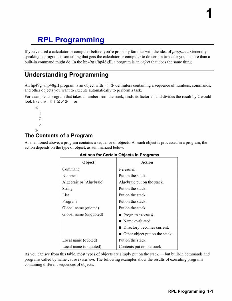
1
RPL Programming 1-1
1.RPL Programming If you've used a calculator or computer before, you're probably familiar with the idea of programs. Generally speaking, a program is something that gets the calculator or computer to do certain tasks for you -- more than a built-in command might do. In the hp49g+/hp48gII, a program is an object that does the same thing.
Understanding Programming An hp49g+/hp48gII program is an object with « » delimiters containing a sequence of numbers, commands, and other objects you want to execute automatically to perform a task. For example, a program that takes a number from the stack, finds its factorial, and divides the result by 2 would look like this: « ! 2 / » or «
!
2
/
»
The Contents of a Program As mentioned above, a program contains a sequence of objects. As each object is processed in a program, the action depends on the type of object, as summarized below.
Actions for Certain Objects in Programs
Object Action Command Executed. Number Put on the stack. Algebraic or `Algebraic` Algebraic put on the stack. String Put on the stack. List Put on the stack. Program Put on the stack. Global name (quoted) Put on the stack. Global name (unquoted) ! Program executed. ! Name evaluated. ! Directory becomes current. ! Other object put on the stack. Local name (quoted) Put on the stack. Local name (unquoted) Contents put on the stack
As you can see from this table, most types of objects are simply put on the stack but built-in commands and programs called by name cause execution. The following examples show the results of executing programs containing different sequences of objects.
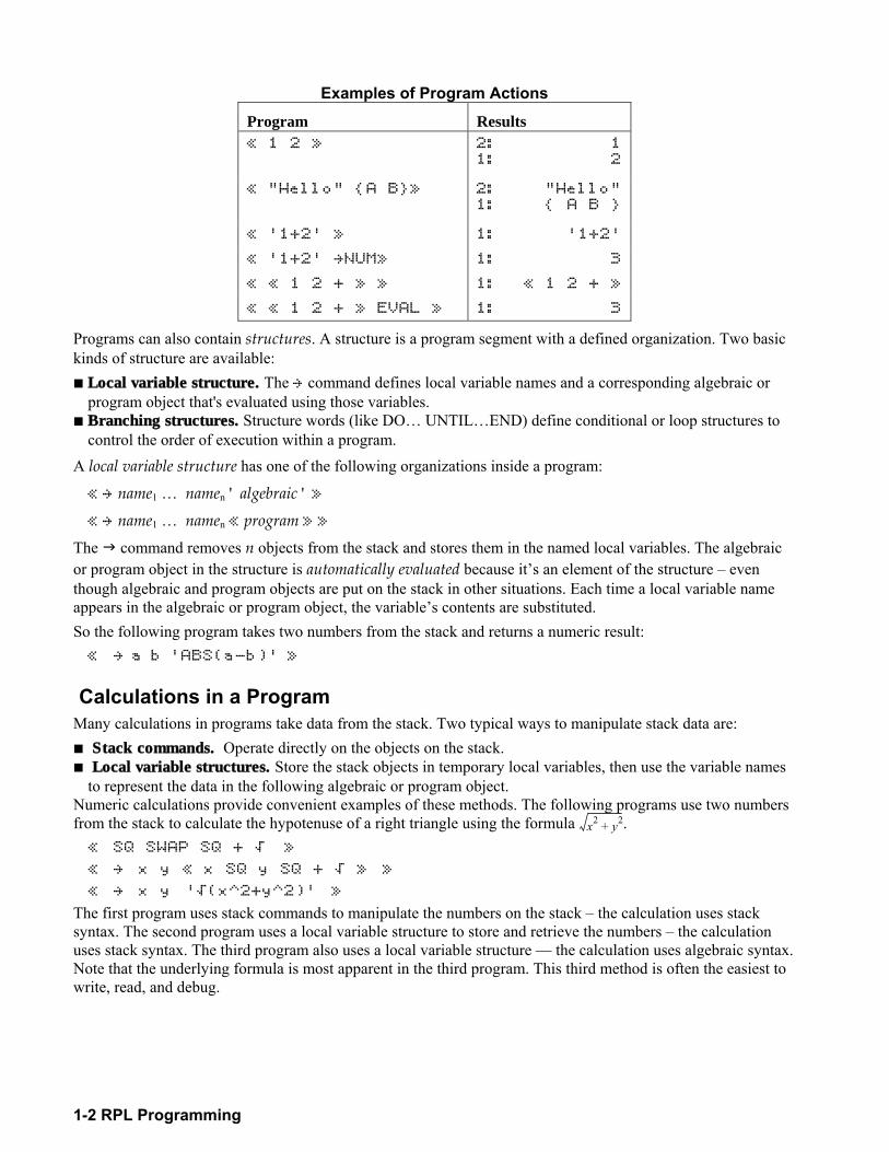
1-2 RPL Programming
x2 y2+
Examples of Program Actions
Program Results « 1 2 » 2: 1
1: 2
« "Hello" A B» 2: "Hello"1: A B
« '1+2' » 1: '1+2'
« '1+2' NUM» 1: 3
« « 1 2 + » » 1: « 1 2 + »
« « 1 2 + » EVAL » 1: 3
Programs can also contain structures. A structure is a program segment with a defined organization. Two basic kinds of structure are available: ! Local variable structure. The command defines local variable names and a corresponding algebraic or
program object that's evaluated using those variables. ! Branching structures. Structure words (like DO UNTILEND) define conditional or loop structures to
control the order of execution within a program. A local variable structure has one of the following organizations inside a program:
« name1 namen ' algebraic ' »
« name1 namen « program » »
The " command removes n objects from the stack and stores them in the named local variables. The algebraic or program object in the structure is automatically evaluated because its an element of the structure even though algebraic and program objects are put on the stack in other situations. Each time a local variable name appears in the algebraic or program object, the variables contents are substituted. So the following program takes two numbers from the stack and returns a numeric result: « a b 'ABS(a-b)' »
Calculations in a Program Many calculations in programs take data from the stack. Two typical ways to manipulate stack data are: ! Stack commands. Operate directly on the objects on the stack. ! Local variable structures. Store the stack objects in temporary local variables, then use the variable names
to represent the data in the following algebraic or program object. Numeric calculations provide convenient examples of these methods. The following programs use two numbers from the stack to calculate the hypotenuse of a right triangle using the formula . « SQ SWAP SQ + ƒ »
« x y « x SQ y SQ + ƒ » »
« x y 'ƒ(x^2+y^2)' »
The first program uses stack commands to manipulate the numbers on the stack the calculation uses stack syntax. The second program uses a local variable structure to store and retrieve the numbers the calculation uses stack syntax. The third program also uses a local variable structure the calculation uses algebraic syntax. Note that the underlying formula is most apparent in the third program. This third method is often the easiest to write, read, and debug.
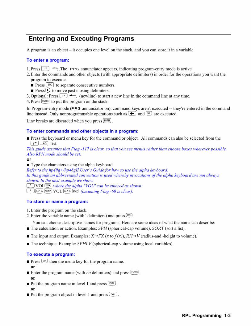
RPL Programming 1-3
Entering and Executing Programs A program is an object it occupies one level on the stack, and you can store it in a variable.
To enter a program:
1. Press @%.The PRG annunciator appears, indicating program-entry mode is active. 2. Enter the commands and other objects (with appropriate delimiters) in order for the operations you want the
program to execute. ! Press # to separate consecutive numbers. ! Press to move past closing delimiters.
3. Optional: Press @ë (newline) to start a new line in the command line at any time. 4. Press ` to put the program on the stack. In Program-entry mode (PRG annunciator on), command keys aren't executed -- they're entered in the command line instead. Only nonprogrammable operations such as and J are executed. Line breaks are discarded when you press `.
To enter commands and other objects in a program: ! Press the keyboard or menu key for the command or object. All commands can also be selected from the
@µ list. This guide assumes that Flag -117 is clear, so that you see menus rather than choose boxes wherever possible. Also RPN mode should be set. or ! Type the characters using the alpha keyboard. Refer to the hp49g+/hp48gII Users Guide for how to use the alpha keyboard. In this guide an abbreviated convention is used whereby invocations of the alpha keyboard are not always shown. In the next example we show: OVOLK where the alpha "VOL" can be entered as shown: O~~VOL ~K (assuming Flag -60 is clear).
To store or name a program:
1. Enter the program on the stack. 2. Enter the variable name (with ' delimiters) and press K.
You can choose descriptive names for programs. Here are some ideas of what the name can describe: ! The calculation or action. Examples: SPH (spherical-cap volume), SORT (sort a list).
! The input and output. Examples: X"FX (x to f (x)), RH"V (radius-and -height to volume).
! The technique. Example: SPHLV (spherical-cap volume using local variables).
To execute a program: ! Press J then the menu key for the program name.
or ! Enter the program name (with no delimiters) and press `.
or ! Put the program name in level 1 and press N.
or ! Put the program object in level 1 and press N.
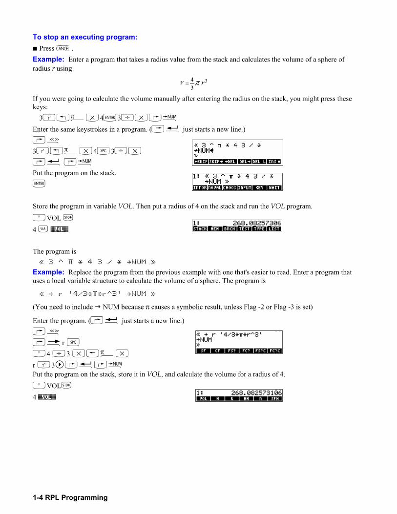
1-4 RPL Programming
To stop an executing program: ! Press −. Example: Enter a program that takes a radius value from the stack and calculates the volume of a sphere of radius r using
3 34 rV π=
If you were going to calculate the volume manually after entering the radius on the stack, you might press these keys: 3Q!ì*4`3/*@ï
Enter the same keystrokes in a program. (@ë just starts a new line.) @% 3Q!ì*4#3/*
@ë @ï Put the program on the stack. ` Store the program in variable VOL. Then put a radius of 4 on the stack and run the VOL program.
OVOL K 4 J %VOL% The program is « 3 ^ œ * 4 3 / * NUM »
Example: Replace the program from the previous example with one that's easier to read. Enter a program that uses a local variable structure to calculate the volume of a sphere. The program is
« r '4/3*œ*r^3' NUM »
(You need to include " NUM because π causes a symbolic result, unless Flag -2 or Flag -3 is set)
Enter the program. (@ë just starts a new line.) @%
@ér #
O4 /3 *!ì*
r Q3 @ë@ï
Put the program on the stack, store it in VOL, and calculate the volume for a radius of 4. OVOLK 4 %VOL%
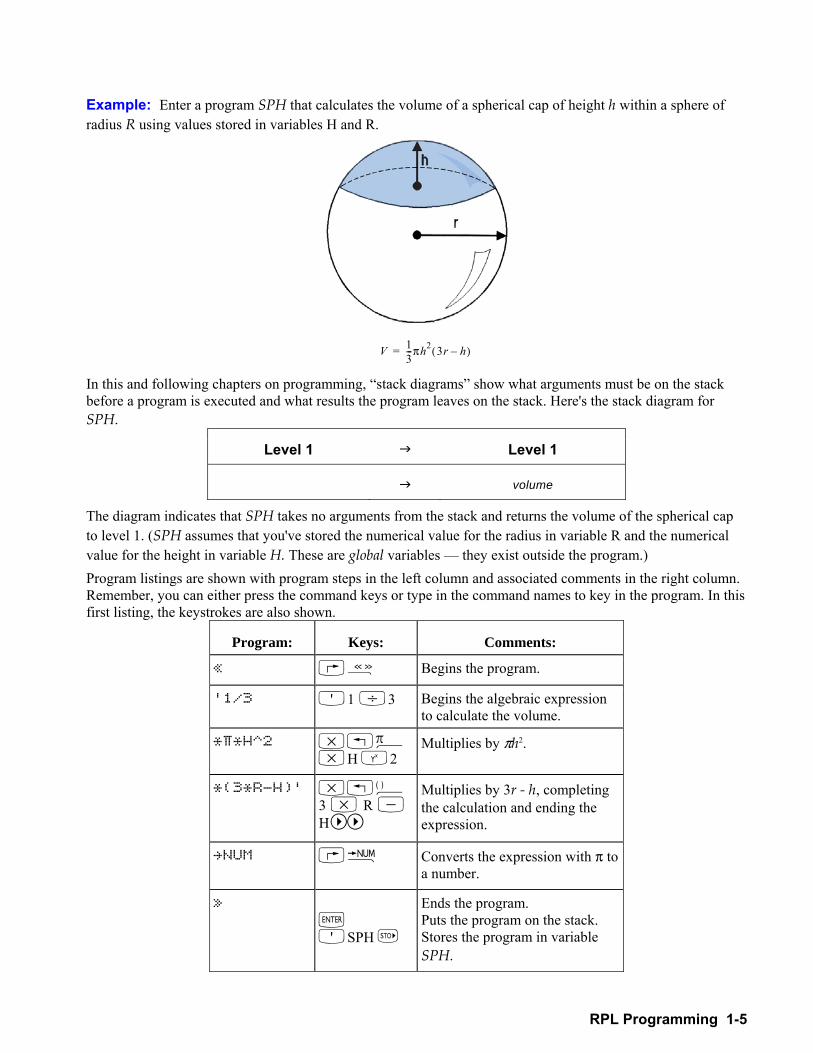
RPL Programming 1-5
Example: Enter a program SPH that calculates the volume of a spherical cap of height h within a sphere of radius R using values stored in variables H and R.
V 13---πh2 3r h( )=
In this and following chapters on programming, stack diagrams show what arguments must be on the stack before a program is executed and what results the program leaves on the stack. Here's the stack diagram for SPH.
Level 1 " Level 1
" volume
The diagram indicates that SPH takes no arguments from the stack and returns the volume of the spherical cap to level 1. (SPH assumes that you've stored the numerical value for the radius in variable R and the numerical value for the height in variable H. These are global variables they exist outside the program.) Program listings are shown with program steps in the left column and associated comments in the right column. Remember, you can either press the command keys or type in the command names to key in the program. In this first listing, the keystrokes are also shown.
Program: Keys: Comments:
« @% Begins the program.
'1/3 O1 /3 Begins the algebraic expression to calculate the volume.
*œ*H^2 *!ì
*H Q2 Multiplies by πh2.
*(3*R-H)' *!Ü3 * R -H
Multiplies by 3r - h, completing the calculation and ending the expression.
NUM @ï Converts the expression with π to a number.
» ` OSPH K
Ends the program. Puts the program on the stack. Stores the program in variable SPH.
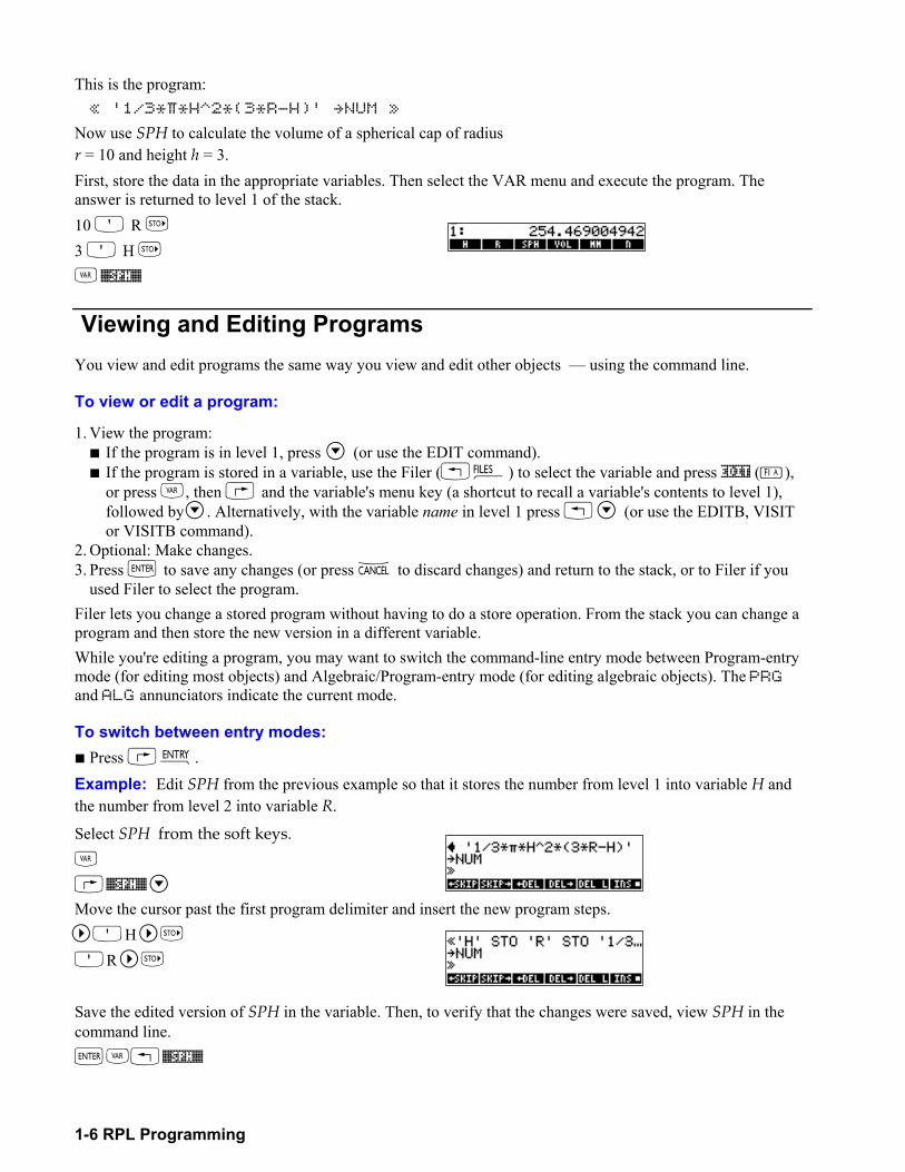
1-6 RPL Programming
This is the program: « '1/3*œ*H^2*(3*R-H)' NUM »
Now use SPH to calculate the volume of a spherical cap of radius r = 10 and height h = 3. First, store the data in the appropriate variables. Then select the VAR menu and execute the program. The answer is returned to level 1 of the stack. 10 O R K 3 O H K J %SPH%
Viewing and Editing Programs You view and edit programs the same way you view and edit other objects using the command line.
To view or edit a program:
1. View the program: ! If the program is in level 1, press (or use the EDIT command). ! If the program is stored in a variable, use the Filer (!¡) to select the variable and press EDIT (),
or press J, then @ and the variable's menu key (a shortcut to recall a variable's contents to level 1), followed by . Alternatively, with the variable name in level 1 press (or use the EDITB, VISIT or VISITB command).
2. Optional: Make changes. 3. Press ` to save any changes (or press − to discard changes) and return to the stack, or to Filer if you
used Filer to select the program. Filer lets you change a stored program without having to do a store operation. From the stack you can change a program and then store the new version in a different variable. While you're editing a program, you may want to switch the command-line entry mode between Program-entry mode (for editing most objects) and Algebraic/Program-entry mode (for editing algebraic objects). The PRG and ALG annunciators indicate the current mode.
To switch between entry modes: ! Press @Í. Example: Edit SPH from the previous example so that it stores the number from level 1 into variable H and the number from level 2 into variable R.
Select SPH from the soft keys. J
@%SPH% Move the cursor past the first program delimiter and insert the new program steps. OH K OR K
Save the edited version of SPH in the variable. Then, to verify that the changes were saved, view SPH in the command line. `J!%SPH%
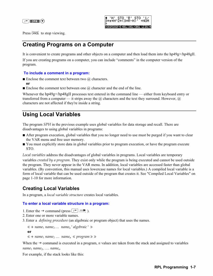
RPL Programming 1-7
@%SPH%
Press − to stop viewing.
Creating Programs on a Computer It is convenient to create programs and other objects on a computer and then load them into the hp49g+/hp48gII. If you are creating programs on a computer, you can include comments in the computer version of the program.
To include a comment in a program: ! Enclose the comment text between two @ characters.
or ! Enclose the comment text between one @ character and the end of the line. Whenever the hp49g+/hp48gII processes text entered in the command line either from keyboard entry or transferred from a computer it strips away the @ characters and the text they surround. However, @ characters are not affected if they're inside a string.
Using Local Variables The program SPH in the previous example uses global variables for data storage and recall. There are disadvantages to using global variables in programs: ! After program execution, global variables that you no longer need to use must be purged if you want to clear
the VAR menu and free user memory. ! You must explicitly store data in global variables prior to program execution, or have the program execute
STO. Local variables address the disadvantages of global variables in programs. Local variables are temporary variables created by a program. They exist only while the program is being executed and cannot be used outside the program. They never appear in the VAR menu. In addition, local variables are accessed faster than global variables. (By convention, this manual uses lowercase names for local variables.) A compiled local variable is a form of local variable that can be used outside of the program that creates it. See "Compiled Local Variables" on page 1-10 for more information.
Creating Local Variables In a program, a local variable structure creates local variables.
To enter a local variable structure in a program:
1. Enter the " command (press @é). 2. Enter one or more variable names. 3. Enter a defining procedure (an algebraic or program object) that uses the names.
« name1 name2 namen ' algebraic ' » or « name1 name2 namen « program » »
When the " command is executed in a program, n values are taken from the stack and assigned to variables name1 name2, . namen. For example, if the stack looks like this:
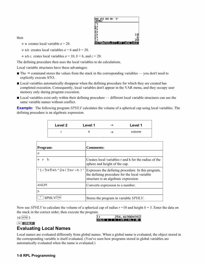
1-8 RPL Programming
then a creates local variable a = 20.
ab creates local variables a = 6 and b = 20.
abc crates local variables a = 10, b = 6, and c = 20. The defining procedure then uses the local variables to do calculations. Local variable structures have these advantages: ! The " command stores the values from the stack in the corresponding variables you don't need to
explicitly execute STO. ! Local variables automatically disappear when the defining procedure for which they are created has
completed execution. Consequently, local variables don't appear in the VAR menu, and they occupy user memory only during program execution.
! Local variables exist only within their defining procedure different local variable structures can use the same variable names without conflict.
Example: The following program SPHLV calculates the volume of a spherical cap using local variables. The defining procedure is an algebraic expression.
Level 2 Level 1 " Level 1 r h " volume
Program: Comments: «
r h Creates local variables r and h for the radius of the sphere and height of the cap.
'1/3*œ*h^2*(3*r-h)' Expresses the defining procedure. In this program, the defining procedure for the local variable structure is an algebraic expression.
NUM Converts expression to a number.
»
OSPHLVK Stores the program in variable SPHLV.
Now use SPHLV to calculate the volume of a spherical cap of radius r =10 and height h = 3. Enter the data on the stack in the correct order, then execute the program. 10 `3 J%SPHLV% Evaluating Local Names Local names are evaluated differently from global names. When a global name is evaluated, the object stored in the corresponding variable is itself evaluated. (You've seen how programs stored in global variables are automatically evaluated when the name is evaluated.)
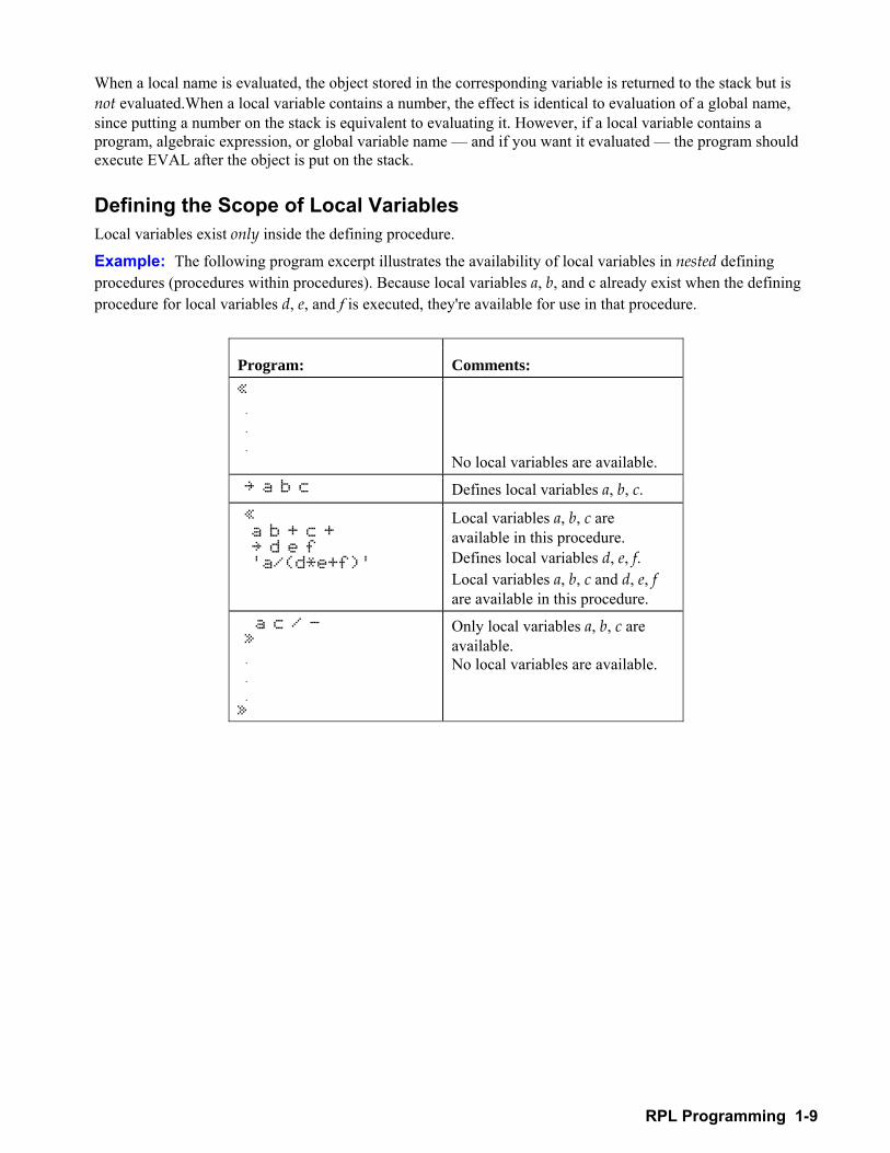
RPL Programming 1-9
When a local name is evaluated, the object stored in the corresponding variable is returned to the stack but is not evaluated.When a local variable contains a number, the effect is identical to evaluation of a global name, since putting a number on the stack is equivalent to evaluating it. However, if a local variable contains a program, algebraic expression, or global variable name and if you want it evaluated the program should execute EVAL after the object is put on the stack. Defining the Scope of Local Variables Local variables exist only inside the defining procedure.
Example: The following program excerpt illustrates the availability of local variables in nested defining procedures (procedures within procedures). Because local variables a, b, and c already exist when the defining procedure for local variables d, e, and f is executed, they're available for use in that procedure.
Program: Comments: « .
.
.
No local variables are available. a b c Defines local variables a, b, c. « a b + c + d e f 'a/(d*e+f)'
Local variables a, b, c are available in this procedure. Defines local variables d, e, f. Local variables a, b, c and d, e, f are available in this procedure.
a c / - »
.
.
. »
Only local variables a, b, c are available. No local variables are available.
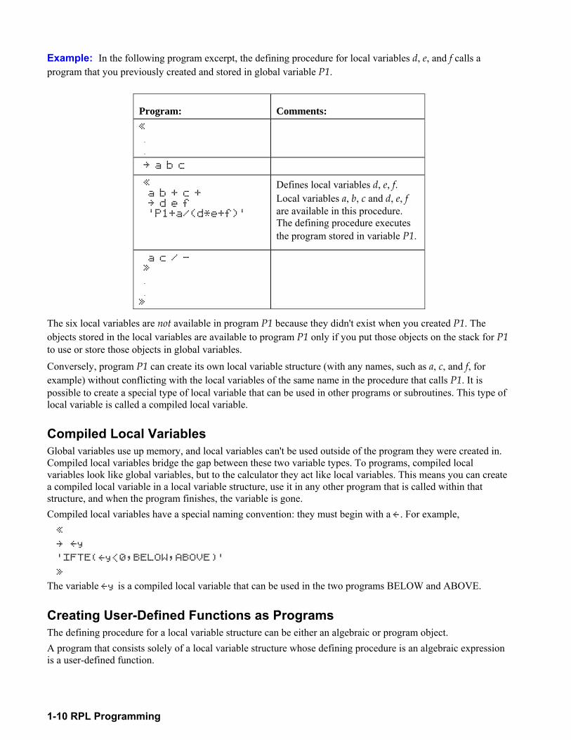
1-10 RPL Programming
Example: In the following program excerpt, the defining procedure for local variables d, e, and f calls a program that you previously created and stored in global variable P1.
Program: Comments: « .
. a b c
« a b + c + d e f 'P1+a/(d*e+f)'
Defines local variables d, e, f. Local variables a, b, c and d, e, f are available in this procedure. The defining procedure executes the program stored in variable P1.
a c / - » .
. »
The six local variables are not available in program P1 because they didn't exist when you created P1. The objects stored in the local variables are available to program P1 only if you put those objects on the stack for P1 to use or store those objects in global variables. Conversely, program P1 can create its own local variable structure (with any names, such as a, c, and f, for example) without conflicting with the local variables of the same name in the procedure that calls P1. It is possible to create a special type of local variable that can be used in other programs or subroutines. This type of local variable is called a compiled local variable. Compiled Local Variables Global variables use up memory, and local variables can't be used outside of the program they were created in. Compiled local variables bridge the gap between these two variable types. To programs, compiled local variables look like global variables, but to the calculator they act like local variables. This means you can create a compiled local variable in a local variable structure, use it in any other program that is called within that structure, and when the program finishes, the variable is gone. Compiled local variables have a special naming convention: they must begin with a Í. For example, «
Íy
'IFTE(Íy<0,BELOW,ABOVE)'
»
The variable Íy is a compiled local variable that can be used in the two programs BELOW and ABOVE. Creating User-Defined Functions as Programs The defining procedure for a local variable structure can be either an algebraic or program object. A program that consists solely of a local variable structure whose defining procedure is an algebraic expression is a user-defined function.
RPL Programming 1-11
If a program begins with a local variable structure and has a program as the defining procedure, the complete program acts like a user-defined function in two ways: it takes numeric or symbolic arguments, and takes those arguments either from the stack or in algebraic syntax. However, it does not have a derivative. (The defining program must, like algebraic defining procedures, return only one result to the stack.) There's an advantage to using a program as the defining procedure for a local variable structure: The program can contain commands not allowed in algebraic expressions. For example, loop structures are not allowed in algebraic expressions.
Using Tests and Conditional Structures You can use commands and branching structures that let programs ask questions and make decisions. Comparison functions and logical functions test whether or not specified conditions exist. Conditional structures and conditional commands use test results to make decisions. Testing Conditions A test is an algebraic or a command sequence that returns a test result to the stack. A test result is either true indicated by a value of 1. or it is false indicated by a value of 0..
To include a test in a program:
! To use stack syntax, enter the two arguments, then enter the test command. ! To use algebraic syntax, enter the test expression (with ' delimiters). You often use test results in conditional structures to determine which clause of the structure to execute. Conditional structures are described under Using Conditional Structures and Commands, p.1-13. Example: Test whether or not X is less than Y. To use stack syntax, enter X Y <. To use algebraic syntax, enter 'X<Y'. (For both cases, if X contains 5 and Y contains 10, then the test is true and 1. is returned to the stack.)
Using Comparison Functions
Comparison functions compare two objects, using either stack syntax or algebraic syntax.
Comparison Functions
Key Programmable Command
Description
° %TEST% (pages 1 and 2):
%$==$%
%%´%%
%#%<%%
%#%>%%
%#%»%%
#%%¼%%
##SAME##
= = ≠ < > ≤ ≥
SAME
Tests equality of two objects. Not equal. Less than. Greater than. Less than or equal to. Greater than or equal to. Identical. Like = =, but doesn't allow a comparison between the numerical value of an algebraic (or name) and a number. Also considers the wordsize of a binary integer.
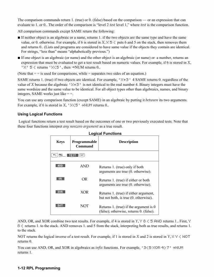
1-12 RPL Programming
The comparison commands return 1. (true) or 0. (false) based on the comparison or an expression that can evaluate to 1. or 0.. The order of the comparison is level 2 test level 1, where test is the comparison function.
All comparison commands except SAME return the following: ! If neither object is an algebraic or a name, returns 1. if the two objects are the same type and have the same
value, or 0. otherwise. For example, if 6 is stored in X, X 5 < puts 6 and 5 on the stack, then removes them and returns 0.. (Lists and programs are considered to have same value if the objects they contain are identical. For strings, less than means alphabetically previous.)
! If one object is an algebraic (or name) and the other object is an algebraic (or name) or a number, returns an expression that must be evaluated to get a test result based on numeric values. For example, if 6 is stored in X, 'X' 5 < returns 'X<5', then "NUM returns 0..
(Note that = = is used for comparisons, while = separates two sides of an equation.) SAME returns 1. (true) if two objects are identical. For example, 'X+3' 4 SAME returns 0. regardless of the value of X because the algebraic 'X+3' is not identical to the real number 4. Binary integers must have the same wordsize and the same value to be identical. For all object types other than algebraics, names, and binary integers, SAME works just like = =. You can use any comparison function (except SAME) in an algebraic by putting it between its two arguments. For example, if 6 is stored in X, 'X<5' NUM returns 0..
Using Logical Functions
Logical functions return a test result based on the outcomes of one or two previously executed tests. Note that these four functions interpret any nonzero argument as a true result.
Logical Functions
Keys Programmable Command
Description
!°%TEST% L
%AND% AND Returns 1. (true) only if both arguments are true (0. otherwise).
%OR% OR Returns 1. (true) if either or both arguments are true (0. otherwise).
%XOR% XOR Returns 1. (true) if either argument, but not both, is true (0. otherwise).
%NOT% NOT Returns 1. (true) if the argument is 0 (false); otherwise, returns 0. (false).
AND, OR, and XOR combine two test results. For example, if 4 is stored in Y, Y 8 < 5 AND returns 1.. First, Y 8 < returns 1. to the stack. AND removes 1. and 5 from the stack, interpreting both as true results, and returns 1. to the stack. NOT returns the logical inverse of a test result. For example, if 1 is stored in X and 2 is stored in Y, X Y < NOT returns 0. You can use AND, OR, and XOR in algebraics as infix functions. For example, '3<5 XOR 4>7' NUM returns 1.
RPL Programming 1-13
You can use NOT as a prefix function in algebraics. For example, 'NOT Z‰4' NUM returns 0. if Z =2.
Testing Object Types
The TYPE command (!°%TEST% L %TYPE%) takes any object as its argument and returns the number that identifies that object type. For example, "HELLO" TYPE returns 2, the value for a string object. See the table of object types in chapter 3, in the TYPE command, to find hp49g+/hp48gII objects and their corresponding type numbers.
Testing Linear Structure
The LININ command (!°%TEST% !«%LININ%) takes an algebraic equation on level 2 and a variable on level 1 as arguments and returns 1. if the equation is linear for that variable, or 0. if it is not. For example, 'H+Y^2' 'H' LININ returns 1. because the equation is structurally linear for H. See the LININ command in chapter 3 for more information. Using Conditional Structures and Commands Conditional structures let a program make a decision based on the results of tests.
Conditional commands let you execute a true-clause or a false-clause (each of which are a single command or object). These conditional structures and commands are contained in the PRG BRCH menu (!°%BRCH%): ! IF THEN END structure. ! IF THEN ELSE END structure. ! CASE END structure. ! IFT (if-then) command. ! IFTE (if-then-else) function.
The IF THEN END Structure
The syntax for this structure is « IF test-clause THEN true-clause END »
IF THEN END executes the sequence of commands in the true-clause only if the test-clause evaluates to true. The test-clause can be a command sequence (for example, A B ‰) or an algebraic (for example,'A‰B'). If the test-clause is an algebraic, it's automatically evaluated to a number you dont need " NUM or EVAL.
IF begins the test-clause, which leaves a test result on the stack. THEN removes the test result from the stack. If the value is nonzero, the true-clause is executed otherwise, program execution resumes following END. See "Conditional Examples" on page 1-15.
To enter IF THEN END in a program:
! Press !°%BRCH% !%IF% .
The IFT Command
The IFT command takes two arguments: a test-result in level 2 and a true-clause object in level 1. If the test-result is true, the true-clause object is executed otherwise, the two arguments are removed from the stack. See "Conditional Examples" on page 1-15.
To enter IFT in a program: ! Press !°%BRCH% L!%IFT% .
1-14 RPL Programming
The IF THEN ELSE END Structure
The syntax for this structure is « IF test-clause THEN true-clause ELSE false-clause END »
IF THEN ELSE END executes either the true-clause sequence of commands if the true-clause is true, or the false-clause sequence of commands if the true-clause is false. If the test-clause is an algebraic, it's automatically evaluated to a number you don't need "NUM or EVAL.
IF begins the test-clause, which leaves a test result on the stack. THEN removes the test result from the stack. If the value is nonzero, the true-clause is executed otherwise, the false-clause is executed. After the appropriate clause is executed, execution resumes following END. See "Conditional Examples" on page 1-15.
To enter IF THEN ELSE END in a program: ! Press !°%BRCH% @%#IF#% .
The IFTE Function
The algebraic syntax for this function is 'IFTE( test, true-clause, false-clause)'
If test evaluates true, the true-clause algebraic is evaluated otherwise, the false-clause algebraic is evaluated. You can also use the IFTE function with stack syntax. It takes three arguments: a test-result in level 3, a true-clause object in level 2, and a false-clause object in level 1. See "Conditional Examples" on page 1-15.
To enter IFTE in a program or in an algebraic: ! Press !°%BRCH% L!%IFTE% .
The CASE END Structure
The syntax for this structure is « CASE
test-clause1 THEN true-clause1 END
test-clause2 THEN truet-clause2 END ... test-clausen THEN true-clausen END
default-clause (optional) END »
The CASE END structure lets you execute a series of test-clause commands, then execute the appropriate true-clause sequence of commands. The first test that returns a true result causes execution of the corresponding true-clause, ending the CASE END structure. Optionally, you can include after the last test a default-clause that's executed if all the tests evaluate to false. If a test-clause is an algebraic, it's automatically evaluated to a number you don't need "NUM or EVAL. When CASE is executed, test-clause1 is evaluated. If the test is true, true-clause1 is executed, and execution skips to END. If test-clause1 is false, execution proceeds to test-clause2. Execution within the CASE structure continues until a true-clause is executed, or until all the test-clauses evaluate to false. If a default clause is included, it's executed if all the test-clauses evaluate to false. See "Conditional Examples" below.
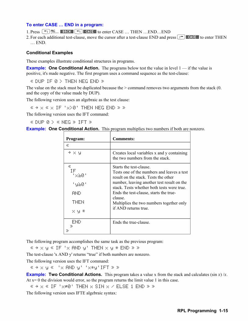
RPL Programming 1-15
To enter CASE END in a program: 1. Press !°%BRCH% !%CASE% to enter CASE THEN ENDEND 2. For each additional test-clause, move the cursor after a test-clause END and press @%CASE% to enter THEN
END.
Conditional Examples
These examples illustrate conditional structures in programs. Example: One Conditional Action. The programs below test the value in level 1 if the value is positive, it's made negative. The first program uses a command sequence as the test-clause:
« DUP IF 0 > THEN NEG END »
The value on the stack must be duplicated because the > command removes two arguments from the stack (0. and the copy of the value made by DUP). The following version uses an algebraic as the test clause:
« x « x IF 'x>0' THEN NEG END » »
The following version uses the IFT command:
« DUP 0 > « NEG » IFT »
Example: One Conditional Action. This program multiplies two numbers if both are nonzero.
Program: Comments: « x y Creates local variables x and y containing
the two numbers from the stack.
« IF 'xŠ0' 'yŠ0' AND THEN x y *
Starts the test-clause. Tests one of the numbers and leaves a test result on the stack. Tests the other number, leaving another test result on the stack. Tests whether both tests were true. Ends the test-clause, starts the true-clause. Multiplies the two numbers together only if AND returns true.
END » »
Ends the true-clause.
The following program accomplishes the same task as the previous program: « x y « IF 'x AND y' THEN x y * END » »
The test-clause 'x AND y' returns true if both numbers are nonzero. The following version uses the IFT command: « x y « 'x AND y' 'x*y'IFT » »
Example: Two Conditional Actions. This program takes a value x from the stack and calculates (sin x) /x. At x= 0 the division would error, so the program returns the limit value 1 in this case. « x « IF 'x‹0' THEN x SIN x / ELSE 1 END » »
The following version uses IFTE algebraic syntax:
1-16 RPL Programming
« x 'IFTE(x‹0,SIN(x)/x,1)' »
Example: Two Conditional Actions. This program multiplies two numbers together if they're both nonzero otherwise, it returns the string ZERO.
Program: Comments: « n1 n2 Creates the local variables.
« IF 'n1‹0 AND n2‹0' THEN n1 n2 * ELSE "ZERO" END
Starts the defining procedure. Starts the test clause. Tests n1 and n2. If both numbers are nonzero, multiplies the two values. Otherwise, returns the string ZERO. Ends the conditional.
» »
Ends the defining procedure.
Example: Two Conditional Actions. This program tests if two numbers on the stack have the same value. If so, it drops one of the numbers and stores the other in variable V1 otherwise, it stores the number from level 1 in V1 and the number from level 2 in V2.
Program: Comments: « IF DUP2 SAME THEN DROP 'V1' STO ELSE 'V1' STO 'V2' STO END
For the test clause, copies the numbers in levels 1 and 2 and tests if they have the same value. For the true clause, drops one of the numbers and stores the other in V1. For the false clause, stores the level 1 number in V1 and the level 2 number in V2. Ends the conditional structure.
»
` OTST K
Puts the program on the stack. Stores it in TST.
Enter the numbers 26 and 52, then execute TST to compare their values. Because the two numbers aren't equal, the VAR menu now contains two new variables V1 and V2.
26 `52 J %TST%
Example: Multiple Conditional Actions. The following program stores the level 1 argument in a variable if the argument is a string, list, or program.
RPL Programming 1-17
Program: Comments: « y «
Defines local variable y. Starts the defining procedure.
CASE y TYPE 2 SAME THEN y 'STR' STO END y TYPE 5 SAME THEN y 'LIST' STO END y TYPE 8 SAME THEN y 'PROG' STO END
Starts the case structure. Case 1: If the argument is a string, stores it in STR. Case 2: If the argument is a list, stores it in LIST. Case 3: If the argument is a program, stores it in PROG.
END »
Ends the case structure. Ends the defining procedure.
»
Using Loop Structures You can use loop structures to execute a part of a program repeatedly. To specify in advance how many times to repeat the loop, use a definite loop. To use a test to determine whether or not to repeat the loop, use an indefinite loop.
Loop structures let a program execute a sequence of commands several times. Loop structures are built with commands called structure words that work only when used in proper combination with each other. These loop structure commands are contained in the PRG BRCH menu (!° %BRCH%): ! START NEXT and START STEP. ! FOR NEXT and FORSTEP ! DO UNTIL END. ! WHILE REPEAT END. In addition, the Σ function provides an alternative to definite loop structures for summations. Using Definite Loop Structures
Each of the two definite loop structures has two variations: ! NEXT. The counter increases by 1 for each loop. ! STEP. The counter increases or decreases by a specified amount for each loop.
The START NEXT Structure
The syntax for this structure is « start finish START loop-clause NEXT »
START NEXT executes the loop-clause sequence of commands one time for each number in the range start to finish. The loop-clause is always executed at least once.
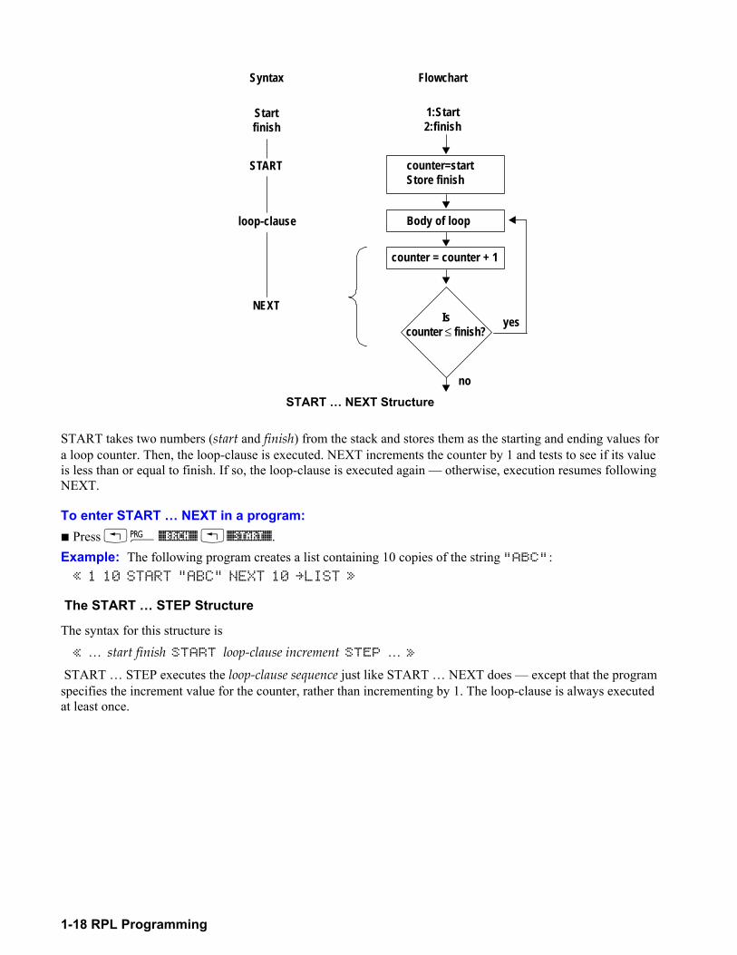
1-18 RPL Programming
Syntax Flowchart
Startfinish
START
loop-clause
NEXT
1:Start2:finish
counter=startStore finish
Body of loop
counter = counter + 1
Iscounter ≤ finish?
yes
no START NEXT Structure
START takes two numbers (start and finish) from the stack and stores them as the starting and ending values for a loop counter. Then, the loop-clause is executed. NEXT increments the counter by 1 and tests to see if its value is less than or equal to finish. If so, the loop-clause is executed again otherwise, execution resumes following NEXT.
To enter START NEXT in a program: ! Press !°%BRCH% !%START%. Example: The following program creates a list containing 10 copies of the string "ABC": « 1 10 START "ABC" NEXT 10 LIST »
The START STEP Structure
The syntax for this structure is « start finish START loop-clause increment STEP »
START STEP executes the loop-clause sequence just like START NEXT does except that the program specifies the increment value for the counter, rather than incrementing by 1. The loop-clause is always executed at least once.
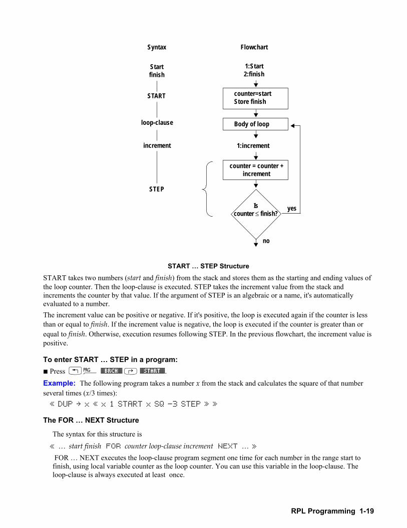
RPL Programming 1-19
Syntax Flowchart
Startfinish
START
loop-clause
STEP
1:Start2:finish
counter=startStore finish
Body of loop
counter = counter +increment
Iscounter ≤ finish?
yes
no
1:incrementincrement
START STEP Structure
START takes two numbers (start and finish) from the stack and stores them as the starting and ending values of the loop counter. Then the loop-clause is executed. STEP takes the increment value from the stack and increments the counter by that value. If the argument of STEP is an algebraic or a name, it's automatically evaluated to a number. The increment value can be positive or negative. If it's positive, the loop is executed again if the counter is less than or equal to finish. If the increment value is negative, the loop is executed if the counter is greater than or equal to finish. Otherwise, execution resumes following STEP. In the previous flowchart, the increment value is positive.
To enter START STEP in a program: ! Press !° %BRCH% %START%. Example: The following program takes a number x from the stack and calculates the square of that number several times (x/3 times): « DUP x « x 1 START x SQ -3 STEP » »
The FOR NEXT Structure
The syntax for this structure is « start finish FOR counter loop-clause increment NEXT »
FOR NEXT executes the loop-clause program segment one time for each number in the range start to finish, using local variable counter as the loop counter. You can use this variable in the loop-clause. The loop-clause is always executed at least once.
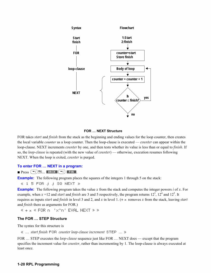
1-20 RPL Programming
Syntax Flowchart
Startfinish
FOR
loop-clause
NEXT
1:Start2:finish
counter=startStore finish
Body of loop
counter = counter + 1
Iscounter ≤ finish?
yes
no
FOR NEXT Structure
FOR takes start and finish from the stack as the beginning and ending values for the loop counter, then creates the local variable counter as a loop counter. Then the loop-clause is executed counter can appear within the loop-clause. NEXT increments counter by one, and then tests whether its value is less than or equal to finish. If so, the loop-clause is repeated (with the new value of counter) otherwise, execution resumes following NEXT. When the loop is exited, counter is purged.
To enter FOR NEXT in a program: ! Press !°%BRCH% ! %FOR%. Example: The following program places the squares of the integers 1 through 5 on the stack: « 1 5 FOR j j SQ NEXT »
Example: The following program takes the value x from the stack and computes the integer powers i of x. For example, when x =12 and start and finish are 3 and 5 respectively, the program returns 123, 124 and 125. It requires as inputs start and finish in level 3 and 2, and x in level 1. ( x removes x from the stack, leaving start and finish there as arguments for FOR.) « x « FOR n 'x^n' EVAL NEXT » »
The FOR STEP Structure
The syntax for this structure is « start finish FOR counter loop-clause increment STEP »
FOR STEP executes the loop-clause sequence just like FOR NEXT does except that the program specifies the increment value for counter, rather than incrementing by 1. The loop-clause is always executed at least once.
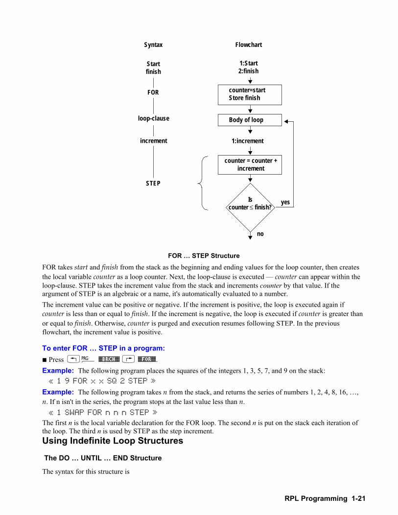
RPL Programming 1-21
Syntax Flowchart
Startfinish
FOR
loop-clause
STEP
1:Start2:finish
counter=startStore finish
Body of loop
counter = counter +increment
Iscounter ≤ finish?
yes
no
1:incrementincrement
FOR STEP Structure
FOR takes start and finish from the stack as the beginning and ending values for the loop counter, then creates the local variable counter as a loop counter. Next, the loop-clause is executed counter can appear within the loop-clause. STEP takes the increment value from the stack and increments counter by that value. If the argument of STEP is an algebraic or a name, it's automatically evaluated to a number. The increment value can be positive or negative. If the increment is positive, the loop is executed again if counter is less than or equal to finish. If the increment is negative, the loop is executed if counter is greater than or equal to finish. Otherwise, counter is purged and execution resumes following STEP. In the previous flowchart, the increment value is positive.
To enter FOR STEP in a program: ! Press !° %BRCH% %FOR%. Example: The following program places the squares of the integers 1, 3, 5, 7, and 9 on the stack: « 1 9 FOR x x SQ 2 STEP »
Example: The following program takes n from the stack, and returns the series of numbers 1, 2, 4, 8, 16, , n. If n isn't in the series, the program stops at the last value less than n. « 1 SWAP FOR n n n STEP »
The first n is the local variable declaration for the FOR loop. The second n is put on the stack each iteration of the loop. The third n is used by STEP as the step increment. Using Indefinite Loop Structures
The DO UNTIL END Structure
The syntax for this structure is
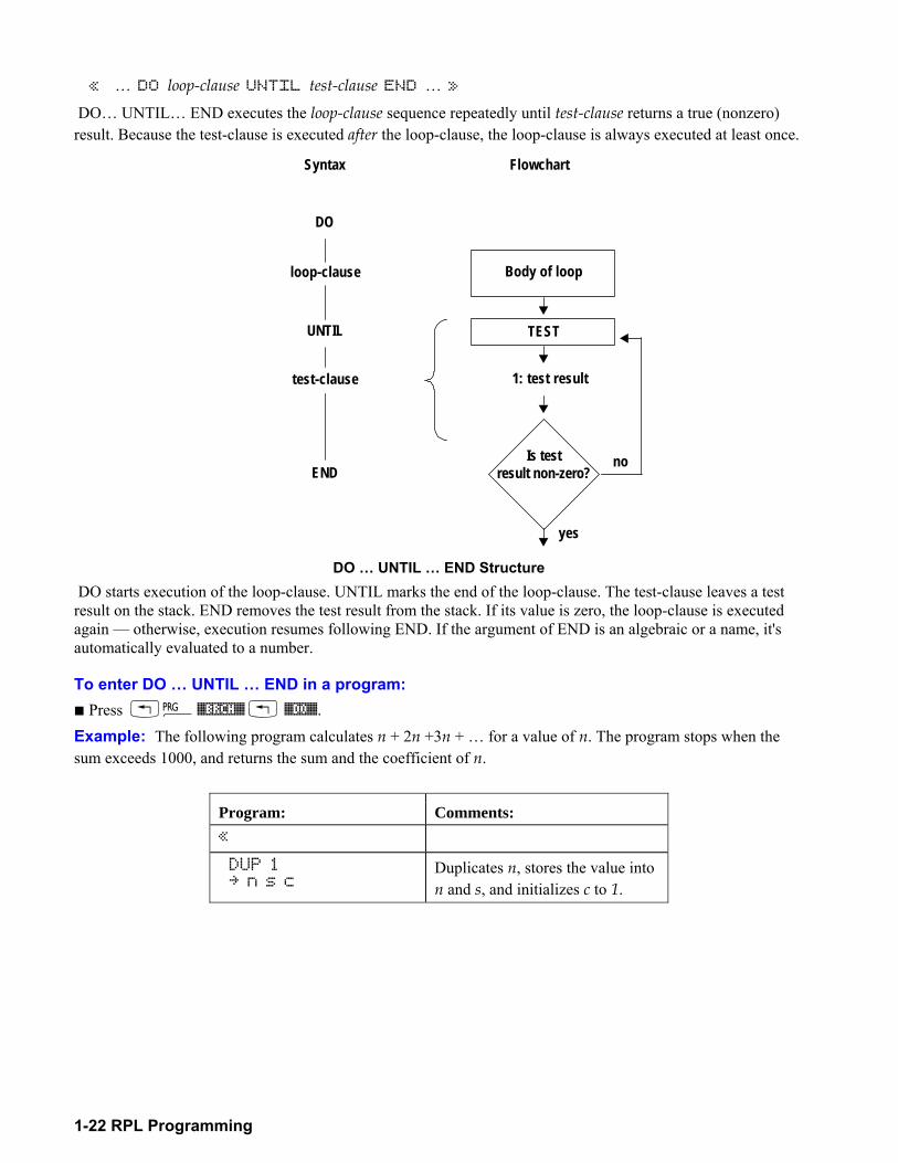
1-22 RPL Programming
« DO loop-clause UNTIL test-clause END »
DO UNTIL END executes the loop-clause sequence repeatedly until test-clause returns a true (nonzero) result. Because the test-clause is executed after the loop-clause, the loop-clause is always executed at least once.
Syntax Flowchart
UNTIL
END
Body of loop
TEST
Is testresult non-zero?
no
yes
1: test resulttest-clause
DO
loop-clause
DO UNTIL END Structure
DO starts execution of the loop-clause. UNTIL marks the end of the loop-clause. The test-clause leaves a test result on the stack. END removes the test result from the stack. If its value is zero, the loop-clause is executed again otherwise, execution resumes following END. If the argument of END is an algebraic or a name, it's automatically evaluated to a number.
To enter DO UNTIL END in a program: ! Press !°%BRCH% ! %DO%. Example: The following program calculates n + 2n +3n + for a value of n. The program stops when the sum exceeds 1000, and returns the sum and the coefficient of n.
Program: Comments: « DUP 1 n s c
Duplicates n, stores the value into n and s, and initializes c to 1.
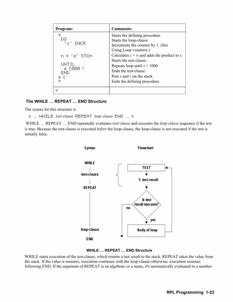
RPL Programming 1-23
Program: Comments: « DO 'c' INCR n * 's' STO+ UNTIL s 1000 > END s c »
Starts the defining procedure. Starts the loop-clause. Increments the counter by 1. (See Using Loop Counters.) Calculates c × n and adds the product to s. Starts the test-clause. Repeats loop until s > 1000. Ends the test-clause. Puts s and c on the stack. Ends the defining procedure.
»
The WHILE REPEAT END Structure
The syntax for this structure is « WHILE test-clause REPEAT loop-clause END »
WHILE REPEAT END repeatedly evaluates test-clause and executes the loop-clause sequence if the test is true. Because the test-clause is executed before the loop-clause, the loop-clause is not executed if the test is initially false.
Syntax Flowchart
REPEAT
END
TEST
Is testresult non-zero?
no
yes
1: test result
loop-clause
WHILE
test-clause
Body of loop
WHILE REPEAT END Structure WHILE starts execution of the test-clause, which returns a test result to the stack. REPEAT takes the value from the stack. If the value is nonzero, execution continues with the loop-clause-otherwise, execution resumes following END. If the argument of REPEAT is an algebraic or a name, it's automatically evaluated to a number.
1-24 RPL Programming
To enter WHILE REPEAT END in a program: ! Press !°%BRCH% ! %WHILE%. Example: The following program starts with a number on the stack, and repeatedly performs a division by 2 as long as the result is evenly divisible. For example, starting with the number 24, the program computes 12, then 6, then 3. « WHILE DUP 2 MOD 0 == REPEAT 2 / DUP END DROP » Example: The following program takes any number of vectors or arrays from the stack and adds them to the statistics matrix. (The vectors and arrays must have the same number of columns.) WHILE REPEAT END is used instead of DO UNTIL END because the test must be done before the addition. (If only vectors or arrays with the same number of columns are on the stack, the program errors after the last vector or array is added to the statistics matrix.) « WHILE DUP TYPE 3 == REPEAT …+ END »
Using Loop Counters For certain problems you may need a counter inside a loop structure to keep track of the number of loops. (This counter isn't related to the counter variable in a FOR NEXT/STEP structure.) You can use any global or local variable as a counter. You can use the INCR or DECR command to increment or decrement the counter value and put its new value on the stack. The syntax for INCR and DECR is « 'variable' INCR » or « 'variable' DECR »
To enter INCR or DECR in a program: ! Press !° #MEM# %ARITH% %INCR% or %DECR%.
The INCR and DECR commands take a global or local variable name (with ' delimiters) as their argument the variable must contain a real number. The command does the following:
1. Changes the value stored in the variable by +1 or -1. 2. Returns the new value to the stack. Examples: If c contains the value 5, then 'c' INCR stores 6 in c and returns 6 to the stack. The following program takes a maximum of five vectors from the stack and adds them to the current statistics matrix.
Program: Comments:« 0 c Stores 0 in local variable c. « WHILE DUP TYPE 3 == 'c' INCR 5 ‰ AND REPEAT …+ END »
Starts the defining procedure. Starts the test clause. Returns true if level 1 contains a vector. Increments and returns the value in c. Returns true if the counter c≤5. Returns true if the two previous test results are true. Adds the vector to ΣDAT. Ends the structure. Ends the defining procedure.
»
RPL Programming 1-25
Using Summations Instead of Loops For certain calculations that involve summations, you can use the Σ function instead of loops. You can use Σ with stack syntax or with algebraic syntax. Σ automatically repeats the addition for the specified range of the index variable without using a loop structure. Example: The following programs take an integer upper limit n from the stack, then find the summation. One program uses a FOR NEXT loop the other uses Σ.
Program: Comments: « 0 1 ROT FOR j j SQ + NEXT
Initializes the summation and puts the limits in place. Loops through the calculation.
»
Program: Comments: « n '…(j=1,n,j^2)'
Uses Σ to calculate the summation.
»
Example: The following program uses ΣLIST to calculate the summation of all elements of a vector or matrix. The program takes from the stack an array or a name that evaluates to an array, and returns the summation.
Program: Comments: « OBJ 1 + œLIST LIST …LIST
Finds the dimensions of the array and leaves it in a list on level 1. Adds 1 to the list. (If the array is a vector, the list on level 1 has only one element. ΠLIST will error if the list has fewer than two elements.) Multiplies all of the list elements together. Converts the array elements into a list, and sums them.
»
Using Flags You can use flags to control calculator behavior and program execution. You can think of a flag as a switch that is either on (set) or off (clear). You can test a flag's state within a conditional or loop structure to make a
j2
j 1=
n
∑
1-26 RPL Programming
decision. Because certain flags have unique meanings for the calculator, flag tests expand a program's decision-making capabilities beyond that available with comparison and logical functions. Types of Flags The hp49g+/hp48gII has two types of flags: ! System flags. Flags -1 through -128. These flags have predefined meanings for the calculator. ! User flags. Flags 1 through 128. User flags are, for the most part, not used by any built-in operations. What
they mean depends entirely on how the program uses them. Appendix C lists the 128 system flags and their definitions. For example, system flag -40 controls the clock display - when this flag is clear (the default state), the clock is not displayed - when this flag is set, the clock is displayed. (When you press %CLK% in the H%MISC% menu, you are setting or clearing flag -40.) Note that for the hp49g+/hp48gII, there are no display annunciators to indicate that user flags 1 through 5 are set, like the hp48S-series and hp48G-series calculators. Setting, Clearing, and Testing Flags Flag commands take a flag number from the stack an integer 1 through 128 (for user flags) or -1 through -128 (for system flags).
To set, clear, or test a flag:
1. Enter the flag number (positive or negative). 2. Execute the flag command see the table below.
Flag Commands
Key Programmable Command
Description
!°%TEST% LL:
%SF% SF Sets the flag.
%CF% CF Clears the flag.
%FS?% FS? Returns 1. (true) if the flag is set, or 0. (false) if the flag is clear.
%FC?% FC? Returns 1. (true) if the flag is clear, or 0. (false) if the flag is set.
%FS?C% FS?C Tests the flag (returns true if the flag is set), then clears the flag.
%FC?C% FC?C Tests the flag (returns true if the flag is clear), then clears the flag.
Example: System Flag. The following program sets an alarm for June 6, 2007 at 5:05 PM. It first tests the status of system flag -42 (Data Format flag) in a conditional structure and then supplies the alarm date in the current date format, based on the test result.
RPL Programming 1-27
Example:
Program: Comments: « IF -42 FC? THEN 6.152007 ELSE 15.062007 END 17.05 "TEST COMPLETE" 3 LIST STOALARM
Tests the status of flag 42, the Date Format flag. If flag 42 is clear, supplies the date in month/day/year format. If flag 42 is set, supplies the date in day.month.year format. Ends the conditional. Sets the alarm: 17.05 is the alarm time and TEST COMPLETE is the alarm message.
»
Example: User Flag. The following program returns either the fractional or integer part of the number in level 1, depending on the state of user flag 10.
Program: Comments: « IF 10 FS? THEN IP ELSE FP END
Starts the conditional. Tests the status of user flag 10. If flag 10 is set, returns the integer part. If flag 10 is clear, returns the fractional part. Ends the conditional.
»
To use this program, you enter a number, either set flag 10 (to get the integer part) or clear flag 10 (to get the fractional part), then run the program. Recalling and Storing the Flag States If you have a program that changes the state of a flag during execution, you may want it to save and restore original flag states. The RCLF (recall flags) and STOF (store flags) commands let you recall and store the states of the hp49g+/hp48gII flags. For these commands, a 64-bit binary integer represents the states of 64 flags each 0 bit corresponds to a flag that's clear, each 1 bit corresponds to a flag that's set. The rightmost (least significant) bit corresponds to system flag 1 or user flag 1 for the lower groups and system flag -65 or user flag 65 for the upper groups.
To recall the current flag states: ! Execute RCLF (!°L %MODES% %FLAG% L%RCLF% ). RCLF returns a list containing four 64-bit binary integers representing the current states of the lower and upper groups of system and user flags: #nsystem-lower #nuser-lower #nsystem-upper #nuser-upper
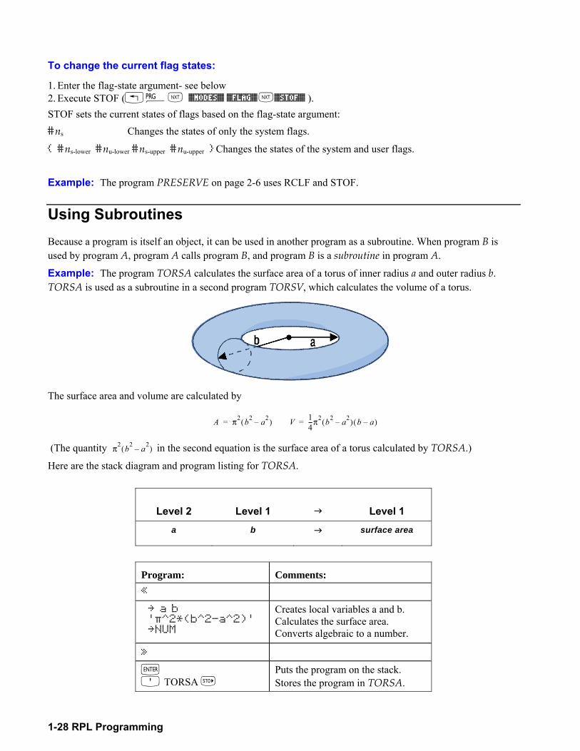
1-28 RPL Programming
To change the current flag states:
1. Enter the flag-state argument- see below 2. Execute STOF (!°L %MODES% %FLAG% L%STOF% ). STOF sets the current states of flags based on the flag-state argument: #ns Changes the states of only the system flags.
#ns-lower #nu-lower #ns-upper #nu-upper Changes the states of the system and user flags.
Example: The program PRESERVE on page 2-6 uses RCLF and STOF.
Using Subroutines Because a program is itself an object, it can be used in another program as a subroutine. When program B is used by program A, program A calls program B, and program B is a subroutine in program A.
Example: The program TORSA calculates the surface area of a torus of inner radius a and outer radius b. TORSA is used as a subroutine in a second program TORSV, which calculates the volume of a torus.
The surface area and volume are calculated by
A π2 b2 a2( )= V 14---π2 b2 a2( ) b a( )=
(The quantity in the second equation is the surface area of a torus calculated by TORSA.)
Here are the stack diagram and program listing for TORSA.
Level 2 Level 1 " Level 1 a b " surface area
Program: Comments: « a b '‡^2*(b^2-a^2)' NUM
Creates local variables a and b. Calculates the surface area. Converts algebraic to a number.
»
`
O TORSA K Puts the program on the stack. Stores the program in TORSA.
π2 b2 a2( )
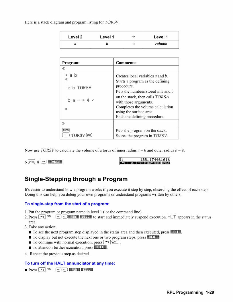
RPL Programming 1-29
Here is a stack diagram and program listing for TORSV.
Level 2 Level 1 " Level 1 a b " volume
Program: Comments:« a b « a b TORSA b a - * 4 / »
Creates local variables a and b. Starts a program as the defining procedure. Puts the numbers stored in a and b on the stack, then calls TORSA with those arguments. Completes the volume calculation using the surface area. Ends the defining procedure.
»
`
O TORSV K Puts the program on the stack. Stores the program in TORSV.
Now use TORSV to calculate the volume of a torus of inner radius a = 6 and outer radius b = 8.
6 ` 8 J %TORSV%
Single-Stepping through a Program It's easier to understand how a program works if you execute it step by step, observing the effect of each step. Doing this can help you debug your own programs or understand programs written by others.
To single-step from the start of a program:
1. Put the program or program name in level 1 ( or the command line). 2. Press !°LL%RUN% %DBUG% to start and immediately suspend execution. HLT appears in the status
area. 3. Take any action: ! To see the next program step displayed in the status area and then executed, press %SST%. ! To display but not execute the next one or two program steps, press %NEXT%. ! To continue with normal execution, press !=. ! To abandon further execution, press %KILL%.
4. Repeat the previous step as desired.
To turn off the HALT annunciator at any time: ! Press !°LL %RUN% %KILL%.
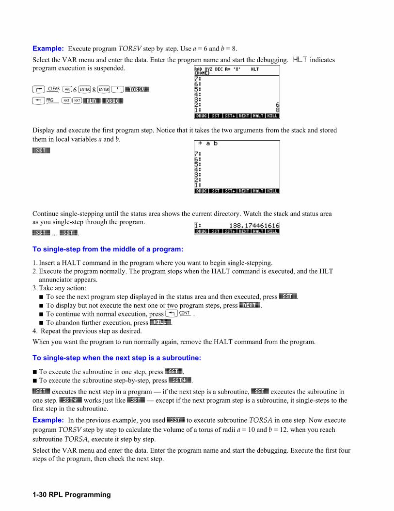
1-30 RPL Programming
Example: Execute program TORSV step by step. Use a = 6 and b = 8. Select the VAR menu and enter the data. Enter the program name and start the debugging. HLT indicates program execution is suspended.
@· J6 `8 `O%TORSV%
!°LL%RUN% %DBUG%
Display and execute the first program step. Notice that it takes the two arguments from the stack and stored them in local variables a and b.
%SST%
Continue single-stepping until the status area shows the current directory. Watch the stack and status area as you single-step through the program. %SST% %SST%.
To single-step from the middle of a program:
1. Insert a HALT command in the program where you want to begin single-stepping. 2. Execute the program normally. The program stops when the HALT command is executed, and the HLT
annunciator appears. 3. Take any action: ! To see the next program step displayed in the status area and then executed, press %SST%. ! To display but not execute the next one or two program steps, press %NEXT%. ! To continue with normal execution, press !=. ! To abandon further execution, press %KILL%.
4. Repeat the previous step as desired. When you want the program to run normally again, remove the HALT command from the program.
To single-step when the next step is a subroutine:
! To execute the subroutine in one step, press %SST%. ! To execute the subroutine step-by-step, press %SST°%. %SST% executes the next step in a program if the next step is a subroutine, %SST% executes the subroutine in one step. %SST°% works just like %SST% except if the next program step is a subroutine, it single-steps to the first step in the subroutine. Example: In the previous example, you used %SST% to execute subroutine TORSA in one step. Now execute program TORSV step by step to calculate the volume of a torus of radii a = 10 and b = 12. when you reach subroutine TORSA, execute it step by step. Select the VAR menu and enter the data. Enter the program name and start the debugging. Execute the first four steps of the program, then check the next step.
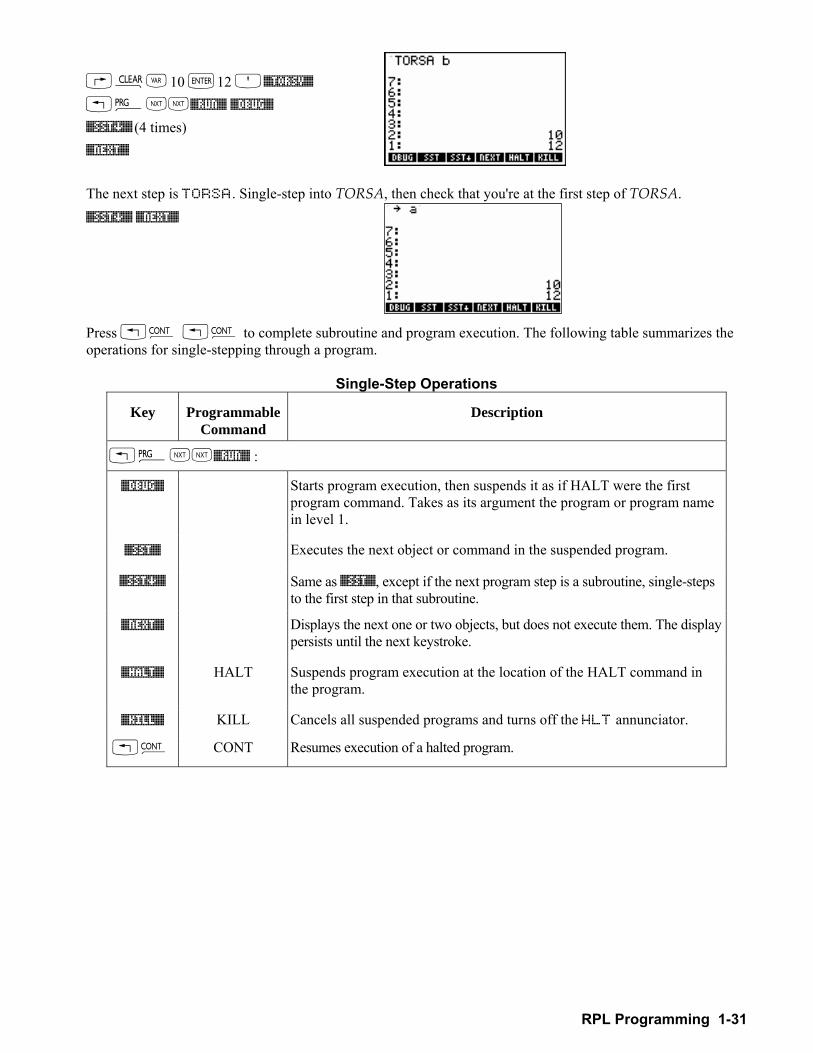
RPL Programming 1-31
@·J 10 `12 O%TORSV%
!°LL%RUN% %DBUG%
%SST°% (4 times) %NEXT% The next step is TORSA. Single-step into TORSA, then check that you're at the first step of TORSA.
%SST°% %NEXT% Press != != to complete subroutine and program execution. The following table summarizes the operations for single-stepping through a program.
Single-Step Operations
Key Programmable Command
Description
!°LL%RUN% :
%DBUG% Starts program execution, then suspends it as if HALT were the first program command. Takes as its argument the program or program name in level 1.
%SST% Executes the next object or command in the suspended program.
%SST°% Same as %SST%, except if the next program step is a subroutine, single-steps to the first step in that subroutine.
%NEXT% Displays the next one or two objects, but does not execute them. The display persists until the next keystroke.
%HALT% HALT Suspends program execution at the location of the HALT command in the program.
%KILL% KILL Cancels all suspended programs and turns off the HLT annunciator.
!= CONT Resumes execution of a halted program.
1-32 RPL Programming
Trapping Errors If you attempt an invalid operation from the keyboard, the operation is not executed and an error message appears. For example, if you execute + with a vector and a real number on the stack, the hp49g+/hp48gII returns the message + Error: Bad Argument Type and returns the arguments to the stack (if Last Arguments is enabled). In a program, the same thing happens, but program execution is also aborted. If you anticipate error conditions, your program can process them without interrupting execution. For simple programs, you can run the program again if it stops with an error. For other programs, you can design them to trap errors and continue executing. You can also create user-defined errors to trap certain conditions in programs. The error trapping commands are located in the PRG ERROR menu. Causing and Analyzing Errors Many conditions are automatically recognized by the hp49g+/hp48gII as error conditions and they're automatically treated as errors in programs. You can also define conditions that cause errors. You can cause a user-defined error (with a user-defined error message) or you can cause a built-in error. Normally, you'll include a conditional or loop structure with a test for the error condition and if it occurs, you'll cause the user-defined or built-in error to occur.
To cause a user-defined error to occur in a program:
1. Enter a string (with "" delimiters) containing the desired error message. 2. Enter the DOERR command (PRG ERROR menu).
To artificially cause a built-in error to occur in a program:
1. Enter the error number (as a binary integer or real number) for the error. 2. Enter the DOERR command (PRG ERROR menu).
If DOERR is trapped in an IFERR structure (described in the next topic), execution continues. If it's not trapped, execution is abandoned at the DOERR command and the error message appears.
To analyze an error in a program:
! To get the error number for the last error, execute ERRN (PRG ERROR menu). ! To get the error message for the last error, execute ERRM (PRG ERROR menu). ! To clear the last-error information, execute ERR0 (PRG ERROR menu). The error number for a user-defined error is #70000h. See the list of built-in error numbers in appendix A, Error and Status Messages. Example: The following program aborts execution if the list in level 1 contains three objects. « OBJ IF 3 == THEN "3 OBJECTS IN LIST" DOERR END »
The following table summarizes error trapping commands.
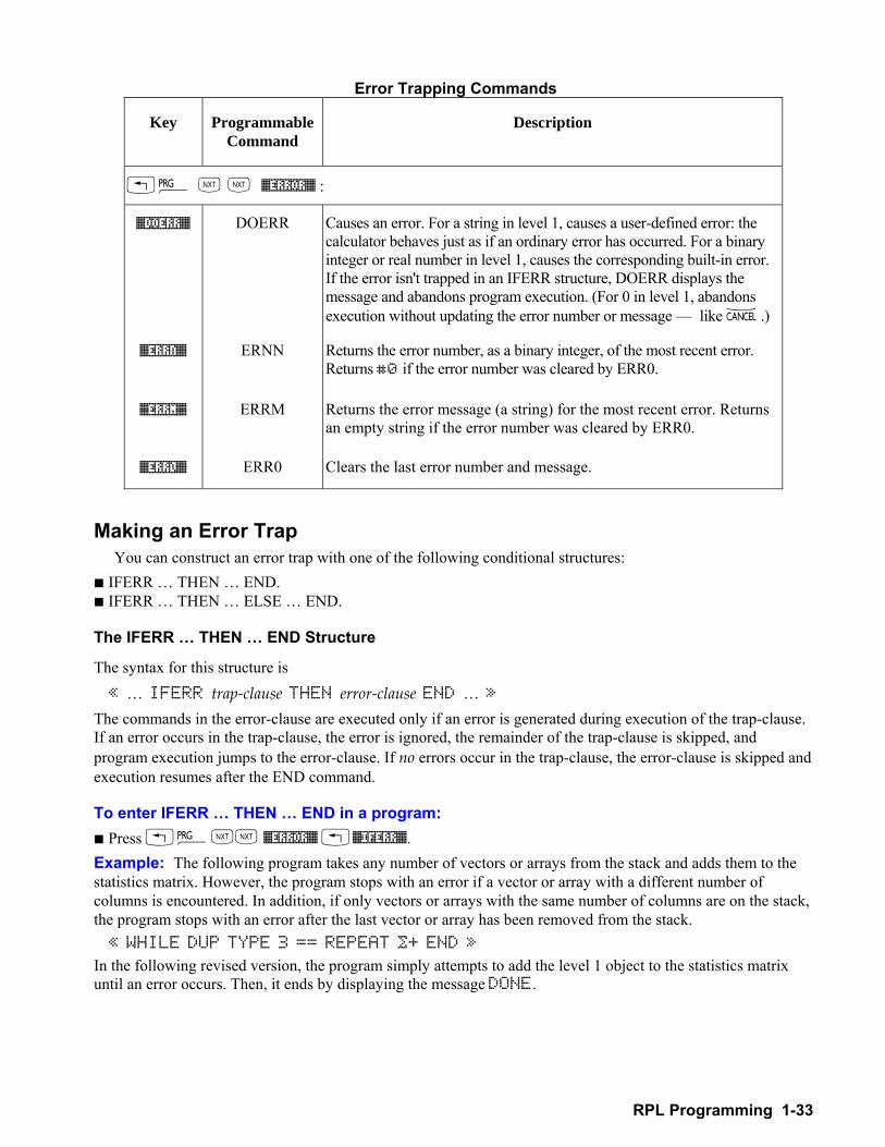
RPL Programming 1-33
Error Trapping Commands
Key Programmable Command
Description
!° L L %ERROR% :
%DOERR% DOERR Causes an error. For a string in level 1, causes a user-defined error: the calculator behaves just as if an ordinary error has occurred. For a binary integer or real number in level 1, causes the corresponding built-in error. If the error isn't trapped in an IFERR structure, DOERR displays the message and abandons program execution. (For 0 in level 1, abandons execution without updating the error number or message like −.)
%ERRN% ERNN Returns the error number, as a binary integer, of the most recent error. Returns #0 if the error number was cleared by ERR0.
%ERRM% ERRM Returns the error message (a string) for the most recent error. Returns an empty string if the error number was cleared by ERR0.
%ERR0% ERR0 Clears the last error number and message.
Making an Error Trap
You can construct an error trap with one of the following conditional structures: ! IFERR THEN END. ! IFERR THEN ELSE END.
The IFERR THEN END Structure
The syntax for this structure is « IFERR trap-clause THEN error-clause END »
The commands in the error-clause are executed only if an error is generated during execution of the trap-clause. If an error occurs in the trap-clause, the error is ignored, the remainder of the trap-clause is skipped, and program execution jumps to the error-clause. If no errors occur in the trap-clause, the error-clause is skipped and execution resumes after the END command.
To enter IFERR THEN END in a program: ! Press !°LL %ERROR% !%IFERR%. Example: The following program takes any number of vectors or arrays from the stack and adds them to the statistics matrix. However, the program stops with an error if a vector or array with a different number of columns is encountered. In addition, if only vectors or arrays with the same number of columns are on the stack, the program stops with an error after the last vector or array has been removed from the stack. « WHILE DUP TYPE 3 == REPEAT …+ END »
In the following revised version, the program simply attempts to add the level 1 object to the statistics matrix until an error occurs. Then, it ends by displaying the message DONE.
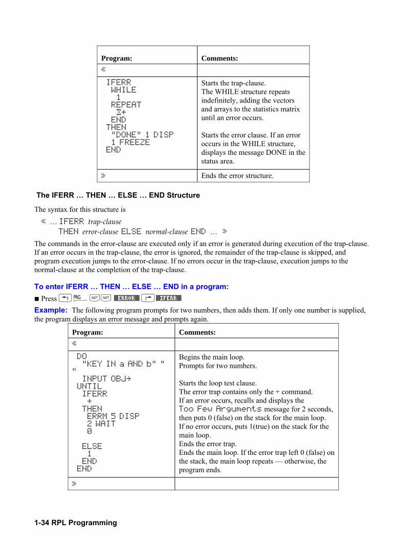
1-34 RPL Programming
Program: Comments: « IFERR WHILE 1 REPEAT …+ END THEN "DONE" 1 DISP 1 FREEZE END
Starts the trap-clause. The WHILE structure repeats indefinitely, adding the vectors and arrays to the statistics matrix until an error occurs. Starts the error clause. If an error occurs in the WHILE structure, displays the message DONE in the status area.
» Ends the error structure.
The IFERR THEN ELSE END Structure
The syntax for this structure is « IFERR trap-clause THEN error-clause ELSE normal-clause END » The commands in the error-clause are executed only if an error is generated during execution of the trap-clause. If an error occurs in the trap-clause, the error is ignored, the remainder of the trap-clause is skipped, and program execution jumps to the error-clause. If no errors occur in the trap-clause, execution jumps to the normal-clause at the completion of the trap-clause.
To enter IFERR THEN ELSE END in a program: ! Press !°LL %ERROR% @%IFERR% Example: The following program prompts for two numbers, then adds them. If only one number is supplied, the program displays an error message and prompts again.
Program: Comments: « DO "KEY IN a AND b" " " INPUT OBJ UNTIL IFERR + THEN ERRM 5 DISP 2 WAIT 0 ELSE 1 END END
Begins the main loop. Prompts for two numbers. Starts the loop test clause. The error trap contains only the + command. If an error occurs, recalls and displays the Too Few Arguments message for 2 seconds, then puts 0 (false) on the stack for the main loop. If no error occurs, puts 1(true) on the stack for the main loop. Ends the error trap. Ends the main loop. If the error trap left 0 (false) on the stack, the main loop repeats otherwise, the program ends.
»
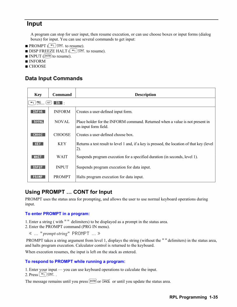
RPL Programming 1-35
Input A program can stop for user input, then resume execution, or can use choose boxes or input forms (dialog boxes) for input. You can use several commands to get input:
! PROMPT (!=to resume). ! DISP FREEZE HALT (!=to resume). ! INPUT (`to resume). ! INFORM ! CHOOSE Data Input Commands
Key Command Description
!°L %IN% :
%INFOR% INFORM Creates a user-defined input form.
%NOVAL NOVAL Place holder for the INFORM command. Returned when a value is not present in an input form field.
%CHOOS% CHOOSE Creates a user-defined choose box.
%KEY% KEY Returns a test result to level 1 and, if a key is pressed, the location of that key (level 2).
%WAIT% WAIT Suspends program execution for a specified duration (in seconds, level 1).
%INPUT% INPUT Suspends program execution for data input.
%PROMP% PROMPT Halts program execution for data input.
Using PROMPT CONT for Input PROMPT uses the status area for prompting, and allows the user to use normal keyboard operations during input.
To enter PROMPT in a program:
1. Enter a string ( with "" delimiters) to be displayed as a prompt in the status area. 2. Enter the PROMPT command (PRG IN menu). « "prompt-string" PROMPT »
PROMPT takes a string argument from level 1, displays the string (without the ""delimiters) in the status area, and halts program execution. Calculator control is returned to the keyboard. When execution resumes, the input is left on the stack as entered.
To respond to PROMPT while running a program:
1. Enter your input you can use keyboard operations to calculate the input. 2. Press !=. The message remains until you press `or − or until you update the status area.
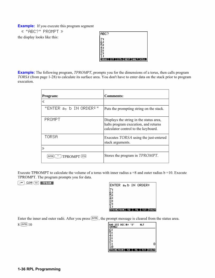
1-36 RPL Programming
Example: If you execute this program segment « "ABC?" PROMPT »
the display looks like this:
Example: The following program, TPROMPT, prompts you for the dimensions of a torus, then calls program TORSA (from page 1-28) to calculate its surface area. You don't have to enter data on the stack prior to program execution.
Program: Comments: « "ENTER a, b IN ORDER:" Puts the prompting string on the stack.
PROMPT Displays the string in the status area, halts program execution, and returns calculator control to the keyboard.
TORSA Executes TORSA using the just-entered stack arguments.
»
`OTPROMPT Stores the program in TPROMPT.
Execute TPROMPT to calculate the volume of a torus with inner radius a =8 and outer radius b =10. Execute TPROMPT. The program prompts you for data. @·J %TPROM%
Enter the inner and outer radii. After you press `, the prompt message is cleared from the status area. 8 `10
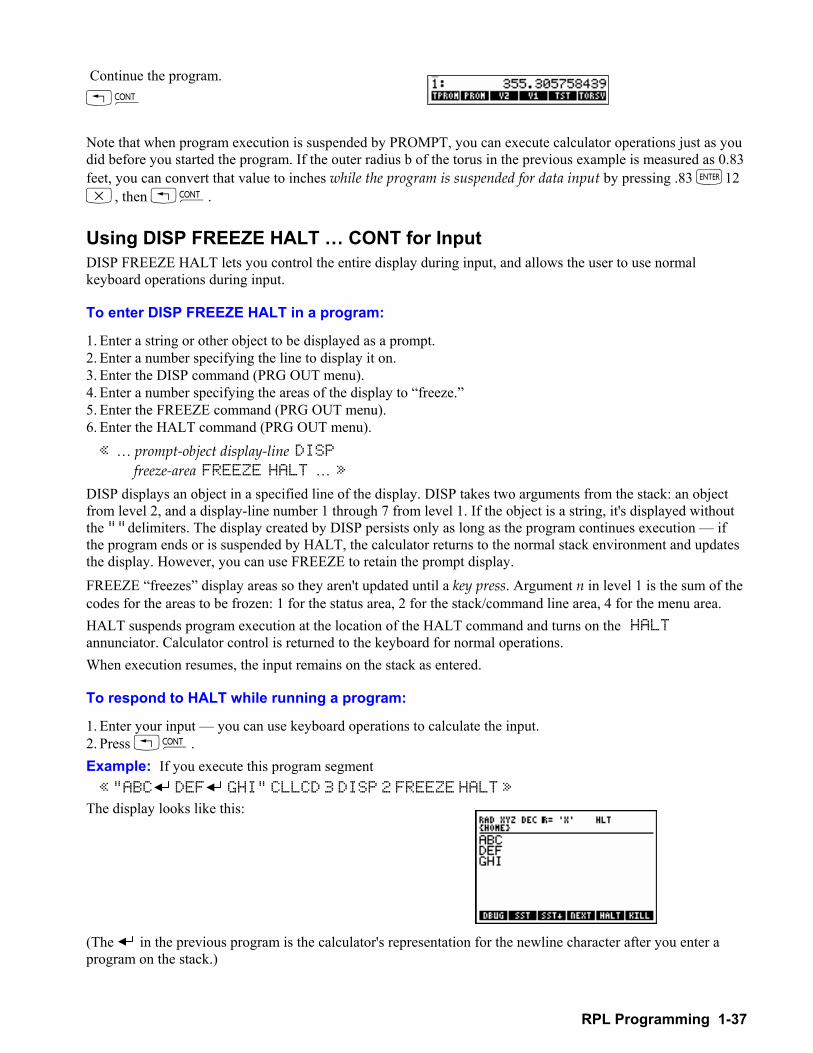
RPL Programming 1-37
Continue the program. != Note that when program execution is suspended by PROMPT, you can execute calculator operations just as you did before you started the program. If the outer radius b of the torus in the previous example is measured as 0.83 feet, you can convert that value to inches while the program is suspended for data input by pressing .83 `12 *, then !=. Using DISP FREEZE HALT CONT for Input DISP FREEZE HALT lets you control the entire display during input, and allows the user to use normal keyboard operations during input.
To enter DISP FREEZE HALT in a program:
1. Enter a string or other object to be displayed as a prompt. 2. Enter a number specifying the line to display it on. 3. Enter the DISP command (PRG OUT menu). 4. Enter a number specifying the areas of the display to freeze. 5. Enter the FREEZE command (PRG OUT menu). 6. Enter the HALT command (PRG OUT menu). « prompt-object display-line DISP freeze-area FREEZE HALT »
DISP displays an object in a specified line of the display. DISP takes two arguments from the stack: an object from level 2, and a display-line number 1 through 7 from level 1. If the object is a string, it's displayed without the ""delimiters. The display created by DISP persists only as long as the program continues execution if the program ends or is suspended by HALT, the calculator returns to the normal stack environment and updates the display. However, you can use FREEZE to retain the prompt display. FREEZE freezes display areas so they aren't updated until a key press. Argument n in level 1 is the sum of the codes for the areas to be frozen: 1 for the status area, 2 for the stack/command line area, 4 for the menu area. HALT suspends program execution at the location of the HALT command and turns on the HALT annunciator. Calculator control is returned to the keyboard for normal operations. When execution resumes, the input remains on the stack as entered.
To respond to HALT while running a program:
1. Enter your input you can use keyboard operations to calculate the input. 2. Press !=. Example: If you execute this program segment « "ABC DEF GHI" CLLCD 3 DISP 2 FREEZE HALT » The display looks like this: (The in the previous program is the calculator's representation for the newline character after you enter a program on the stack.)
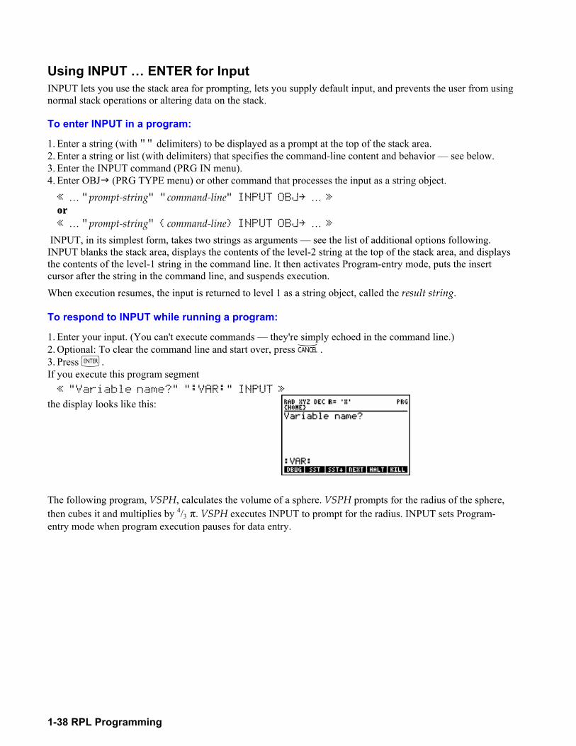
1-38 RPL Programming
Using INPUT ENTER for Input INPUT lets you use the stack area for prompting, lets you supply default input, and prevents the user from using normal stack operations or altering data on the stack.
To enter INPUT in a program:
1. Enter a string (with "" delimiters) to be displayed as a prompt at the top of the stack area. 2. Enter a string or list (with delimiters) that specifies the command-line content and behavior see below. 3. Enter the INPUT command (PRG IN menu). 4. Enter OBJ" (PRG TYPE menu) or other command that processes the input as a string object. « "prompt-string" "command-line" INPUT OBJ » or « "prompt-string" command-line INPUT OBJ »
INPUT, in its simplest form, takes two strings as arguments see the list of additional options following. INPUT blanks the stack area, displays the contents of the level-2 string at the top of the stack area, and displays the contents of the level-1 string in the command line. It then activates Program-entry mode, puts the insert cursor after the string in the command line, and suspends execution. When execution resumes, the input is returned to level 1 as a string object, called the result string.
To respond to INPUT while running a program:
1. Enter your input. (You can't execute commands they're simply echoed in the command line.) 2. Optional: To clear the command line and start over, press −. 3. Press `. If you execute this program segment « "Variable name?" ":VAR:" INPUT »
the display looks like this: The following program, VSPH, calculates the volume of a sphere. VSPH prompts for the radius of the sphere, then cubes it and multiplies by 4/3 π. VSPH executes INPUT to prompt for the radius. INPUT sets Program-entry mode when program execution pauses for data entry.
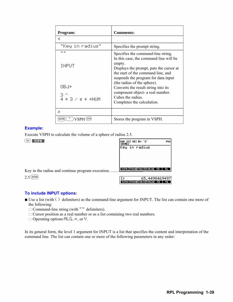
RPL Programming 1-39
Program: Comments: « "Key in radius" Specifies the prompt string.
"" INPUT OBJ 3 ^ 4 * 3 / ‡ * NUM
Specifies the command-line string. In this case, the command line will be empty. Displays the prompt, puts the cursor at the start of the command line, and suspends the program for data input (the radius of the sphere). Converts the result string into its component object- a real number. Cubes the radius. Completes the calculation.
»
`OVSPH Stores the program in VSPH.
Example: Execute VSPH to calculate the volume of a sphere of radius 2.5. J %VSPH%
Key in the radius and continue program execution. ............................... 2.5 `
To include INPUT options: ! Use a list (with delimiters) as the command-line argument for INPUT. The list can contain one more of
the following: " Command-line string (with "" delimiters). " Cursor position as a real number or as a list containing two real numbers. " Operating options ALG, Œ, or V.
In its general form, the level 1 argument for INPUT is a list that specifies the content and interpretation of the command line. The list can contain one or more of the following parameters in any order:
1-40 RPL Programming
"command-line" cursor-position operating-options
Command-line
Specifies the content of the command line when the program pauses. Embedded newline characters produce multiple lines in the display. (If not included, the command line is blank.)
Cursor-position
Specifies the position of the cursor in the command line and its type. (If not included, an insert cursor is at the end of the command line.)
! A real number n specifies the nth character in the first row (line) of the command line. Zero specifies the end of the command-line string. A positive number specifies the insert cursor a negative number specifies the replace cursor.
! A list row character specifies the row and character position. Row 1 is the first row(line) of the command line. Characters count from the left end of each row character 0 specifies the end of the row. A positive row number specifies the insert cursor a negative row number specifies the replace cursor.
operating-options
Specify the input setup and processing using zero or more of these unquoted names: ! ALG activates Algebraic/Program-entry mode (for algebraic syntax). (If not included,
Program-entry mode is active.) ! Π(~a) specifies alpha lock. (If not included, alpha is inactive.) ! V verifies whether the result string (without the ""delimiters) is a valid object or
sequence of objects. If the result string isn't valid, INPUT displays the Invalid Syntax message and prompts again for data. (if not included, syntax isn't checked.)
To design the command-line string for INPUT:
! For simple input, use a string that produces a valid object: " Use an empty string " Use a :label : tag. " Use a @ text @ comment.
! For special input, use a string that produces a recognizable pattern. After the user enters input in the command line and presses ` to resume execution, the contents of the command line are returned to level 1 as the result string. The result string normally contains the original command-line string, too. If you design the command-line string carefully, you can ease the process of extracting the input data.
To process the result string from INPUT:
! For simple input, use OBJ" to convert the string into its corresponding objects. ! For sensitive input, use the V option for INPUT to check for valid objects, then use OBJ" to convert the
string into those objects. ! For special input, process the input as a string object, possibly extracting data as substrings. Example: The program VSPH on page 1-39 uses an empty command-line string.
Example: The program SSEC on page 1-42 uses a command-line string whose characters form a pattern. The program extracts substrings from the result string.
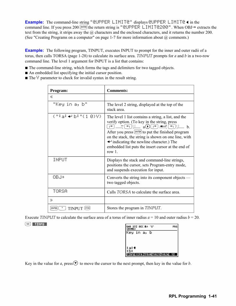
RPL Programming 1-41
Example: The command-line string "@UPPER LIMIT@" displays @UPPER LIMIT@´ in the command line. If you press 200 `the return string is "@UPPER LIMIT@200". When OBJ" extracts the text from the string, it strips away the @ characters and the enclosed characters, and it returns the number 200. (See "Creating Programs on a computer" on page 1-7 for more information about @ comments.) Example: The following program, TINPUT, executes INPUT to prompt for the inner and outer radii of a torus, then calls TORSA (page 1-28) to calculate its surface area. TINPUT prompts for a and b in a two-row command line. The level 1 argument for INPUT is a list that contains: ! The command-line string, which forms the tags and delimiters for two tagged objects. ! An embedded list specifying the initial cursor position. ! The V parameter to check for invalid syntax in the result string.
Program: Comments: « "Key in a, b" The level 2 string, displayed at the top of the
stack area.
":a: b:"1 0V The level 1 list contains a string, a list, and the verify option. (To key in the string, press @Õ!ê a @ë!ê b. After you press `to put the finished program on the stack, the string is shown on one line, with
indicating the newline character.) The embedded list puts the insert cursor at the end of row 1.
INPUT Displays the stack and command-line strings, positions the cursor, sets Program-entry mode, and suspends execution for input.
OBJ Converts the string into its component objects two tagged objects.
TORSA Calls TORSA to calculate the surface area.
»
`O TINPUT Stores the program in TINPUT.
Execute TINPUT to calculate the surface area of a torus of inner radius a = 10 and outer radius b = 20.
J %TINPU% Key in the value for a, press to move the cursor to the next prompt, then key in the value for b.
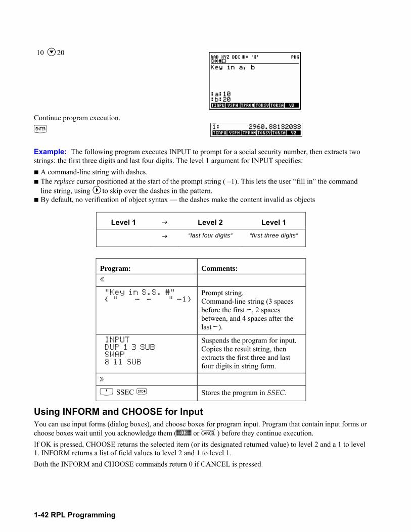
1-42 RPL Programming
10 20
Continue program execution. `
Example: The following program executes INPUT to prompt for a social security number, then extracts two strings: the first three digits and last four digits. The level 1 argument for INPUT specifies: ! A command-line string with dashes. ! The replace cursor positioned at the start of the prompt string ( 1). This lets the user fill in the command
line string, using to skip over the dashes in the pattern. ! By default, no verification of object syntax the dashes make the content invalid as objects
Level 1 " Level 2 Level 1 " “last four digits“ “first three digits“
Program: Comments: « "Key in S.S. #" " - - " -1
Prompt string. Command-line string (3 spaces before the first -, 2 spaces between, and 4 spaces after the last -).
INPUT DUP 1 3 SUB SWAP 8 11 SUB
Suspends the program for input. Copies the result string, then extracts the first three and last four digits in string form.
»
O SSEC Stores the program in SSEC.
Using INFORM and CHOOSE for Input You can use input forms (dialog boxes), and choose boxes for program input. Program that contain input forms or choose boxes wait until you acknowledge them (%OK% or −) before they continue execution. If OK is pressed, CHOOSE returns the selected item (or its designated returned value) to level 2 and a 1 to level 1. INFORM returns a list of field values to level 2 and 1 to level 1. Both the INFORM and CHOOSE commands return 0 if CANCEL is pressed.
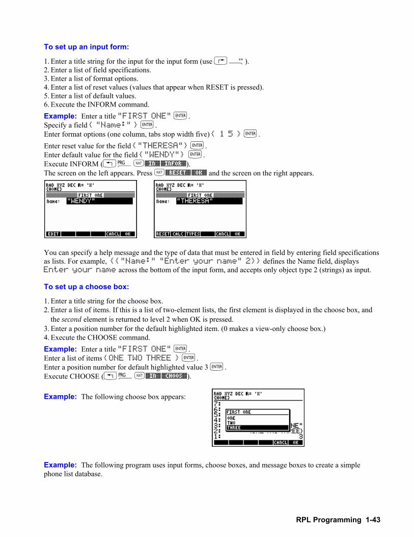
RPL Programming 1-43
To set up an input form:
1. Enter a title string for the input for the input form (use @Õ). 2. Enter a list of field specifications. 3. Enter a list of format options. 4. Enter a list of reset values (values that appear when RESET is pressed). 5. Enter a list of default values. 6. Execute the INFORM command. Example: Enter a title "FIRST ONE" `. Specify a field "Name:" `. Enter format options (one column, tabs stop width five) 1 5 `. Enter reset value for the field "THERESA" `. Enter default value for the field "WENDY" `. Execute INFORM (!°L%IN% %INFOR%). The screen on the left appears. Press L%RESET% %OK% and the screen on the right appears.
You can specify a help message and the type of data that must be entered in field by entering field specifications as lists. For example, "Name:" "Enter your name" 2 defines the Name field, displays Enter your name across the bottom of the input form, and accepts only object type 2 (strings) as input.
To set up a choose box:
1. Enter a title string for the choose box. 2. Enter a list of items. If this is a list of two-element lists, the first element is displayed in the choose box, and
the second element is returned to level 2 when OK is pressed. 3. Enter a position number for the default highlighted item. (0 makes a view-only choose box.) 4. Execute the CHOOSE command. Example: Enter a title "FIRST ONE" `. Enter a list of items ONE TWO THREE `. Enter a position number for default highlighted value 3 `. Execute CHOOSE (!°L%IN% %CHOOS%). Example: The following choose box appears:
Example: The following program uses input forms, choose boxes, and message boxes to create a simple phone list database.
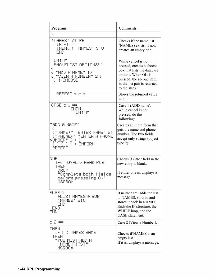
1-44 RPL Programming
Program: Comments: « 'NAMES' VTYPE IF -1 == THEN 'NAMES' STO END
Checks if the name list (NAMES) exists, if not, creates an empty one.
WHILE "PHONELIST OPTIONS:" "ADD A NAME" 1 "VIEW A NUMBER" 2 1 CHOOSE
While cancel is not pressed, creates a choose box that lists the database options. When OK is pressed, the second item in the list pair is returned to the stack.
REPEAT c « Stores the returned value in c.
CASE c 1 == THEN WHILE
Case 1 (ADD name), while cancel is not pressed, do the following:
"ADD A NAME" "NAME:" "ENTER NAME" 2 "PHONE:" "ENTER A PHONE NUMBER" 2 INFORM REPEAT
Creates an input form that gets the name and phone number. The two fields accept only strings (object type 2).
DUP IF NOVAL HEAD POS THEN DROP "Complete both fields before pressing OK" MSGBOX
Checks if either field in the new entry is blank. If either one is, displays a message.
ELSE 1 LIST NAMES + SORT 'NAMES' STO END END END
If neither are, adds the list to NAMES, sorts it, and stores it back in NAMES. Ends the IF structure, the WHILE loop, and the CASE statement.
c 2 == Case 2 (View a Number).
THEN IF NAMES SAME THEN "YOU MUST ADD A NAME FIRST" MSGBOX
Checks if NAMES is an empty list. If it is, displays a message.
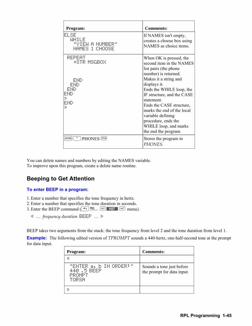
RPL Programming 1-45
Program: Comments: ELSE WHILE "VIEW A NUMBER" NAMES 1 CHOOSE
If NAMES isn't empty, creates a choose box using NAMES as choice items.
REPEAT STR MSGBOX END END END END » END »
When OK is pressed, the second item in the NAMES list pairs (the phone number) is returned. Makes it a string and displays it. Ends the WHILE loop, the IF structure, and the CASE statement. Ends the CASE structure, marks the end of the local variable defining procedure, ends the WHILE loop, and marks the end the program.
`OPHONES Stores the program in PHONES.
You can delete names and numbers by editing the NAMES variable. To improve upon this program, create a delete name routine. Beeping to Get Attention
To enter BEEP in a program:
1. Enter a number that specifies the tone frequency in hertz. 2. Enter a number that specifies the tone duration in seconds. 3. Enter the BEEP command (!°L%OUT% L menu). « frequency duration BEEP »
BEEP takes two arguments from the stack: the tone frequency from level 2 and the tone duration from level 1. Example: The following edited version of TPROMPT sounds a 440-hertz, one-half-second tone at the prompt for data input.
Program: Comments: « "ENTER a, b IN ORDER:" 440 .5 BEEP PROMPT TORSA
Sounds a tone just before the prompt for data input.
»
1-46 RPL Programming
Stopping a Program for Keystroke Input A program can stop for keystroke input it can wait for the user to press a key. You can do this with the WAIT and KEY commands. Using WAIT for Keystroke Input The WAIT command normally suspends execution for a specified number of seconds. However, you can specify that it wait indefinitely until a key is pressed.
To enter WAIT in a program:
! To stop without changing the display, enter 0 and the WAIT command (PRG IN menu). ! To stop and display the current menu, enter 1 and the WAIT command (PRG IN menu). WAIT takes the 0 or 1 from level 1, then suspends execution until a valid keystroke is executed. For an argument of 1, WAIT displays the currently specified menu. This lets you build and display a menu of user choices while the program is paused. (A menu built with MENU or TMENU is not normally displayed until the program ends or is halted.) When execution resumes, the three-digit key location number of the pressed key is left on the stack. This number indicates the row, column, and shift level of the key.
To respond to WAIT while running a program: ! Press any valid keystroke. (A prefix key such as !or ~ by itself is not a valid keystroke.) Using KEY for Keystroke Input You can use KEY inside an indefinite loop to pause execution until any key or a certain key is pressed.
To enter a KEY loop in a program:
1. Enter the loop structure. 2. In the test-clause sequence, enter the KEY command (PRG IN menu) plus any necessary test commands. 3. In the loop-clause, enter no commands to give the appearance of a paused condition. KEY returns 0 to level 1 when the loop begins. It continues to return 0 until a key is pressed then it returns 1 to level 1 and the two-digit row-column number of the pressed key to level 2. For example, `returns 105, and ! returns 81.) The test-clause should normally cause the loop to repeat until a key is pressed. If a key is pressed, you can use comparison tests to check the value of the key number. (See "Using Indefinite Loop Structures" on page 1-21 and "Using Comparison Functions" on page 1-11.)
To respond to a KEY loop while running a program:
! Press any key. (A prefix key such as !or ~is a valid key.) Example: The following program segment returns 1 to level 1 if + is pressed, or 0 to level 1 if any other key is pressed: « DO UNTIL KEY END 95 SAME »
Output You can determine how a program presents its output. You can make the output more recognizable using the techniques described in this section.
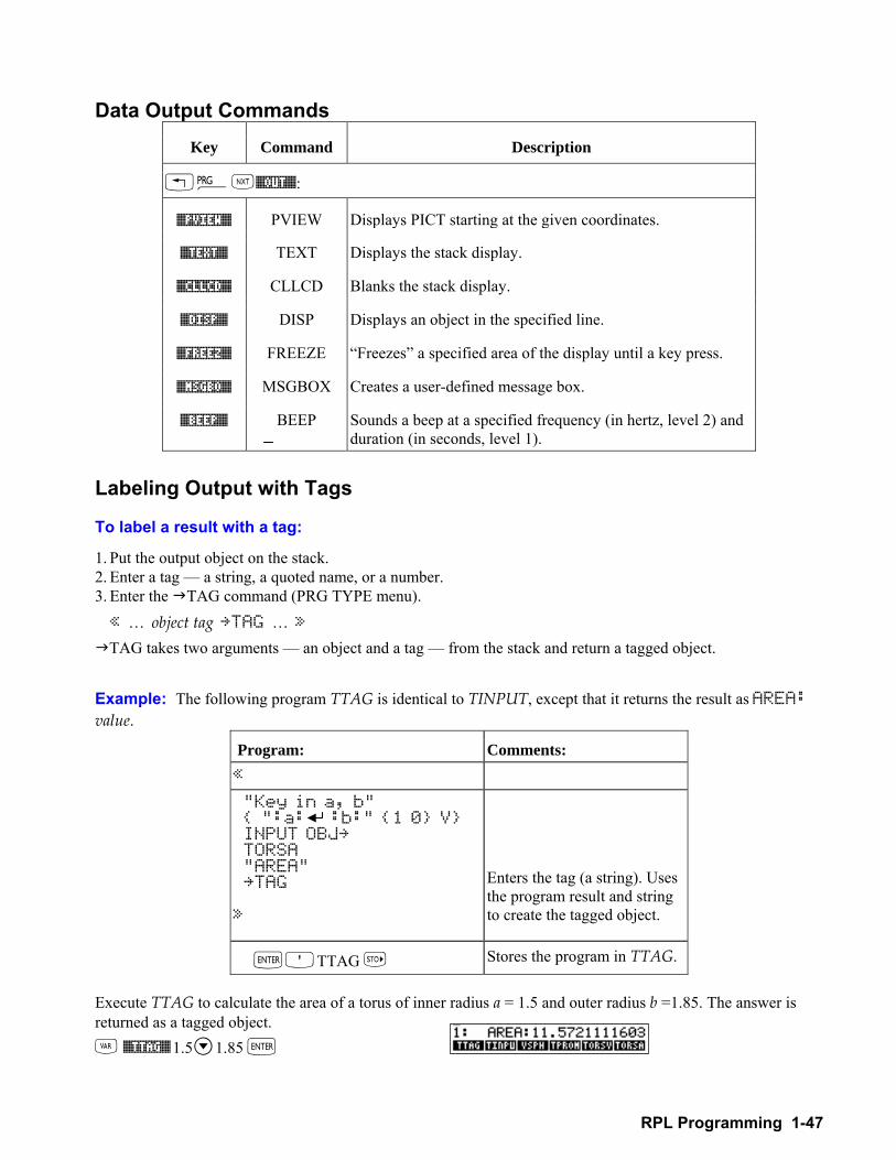
RPL Programming 1-47
Data Output Commands
Key Command Description
!°L%OUT%:
%PVIEW% PVIEW Displays PICT starting at the given coordinates.
%TEXT% TEXT Displays the stack display.
%CLLCD% CLLCD Blanks the stack display.
%DISP% DISP Displays an object in the specified line.
%FREEZ% FREEZE Freezes a specified area of the display until a key press.
%MSGBO% MSGBOX Creates a user-defined message box.
%BEEP% BEEP Sounds a beep at a specified frequency (in hertz, level 2) and duration (in seconds, level 1).
Labeling Output with Tags
To label a result with a tag:
1. Put the output object on the stack. 2. Enter a tag a string, a quoted name, or a number. 3. Enter the "TAG command (PRG TYPE menu). « object tag TAG »
"TAG takes two arguments an object and a tag from the stack and return a tagged object. Example: The following program TTAG is identical to TINPUT, except that it returns the result as AREA: value.
Program: Comments: «
"Key in a, b" ":a: :b:" 1 0 V INPUT OBJ TORSA "AREA" TAG »
Enters the tag (a string). Uses the program result and string to create the tagged object.
`OTTAG Stores the program in TTAG.
Execute TTAG to calculate the area of a torus of inner radius a = 1.5 and outer radius b =1.85. The answer is returned as a tagged object. J %TTAG% 1.5 1.85 `
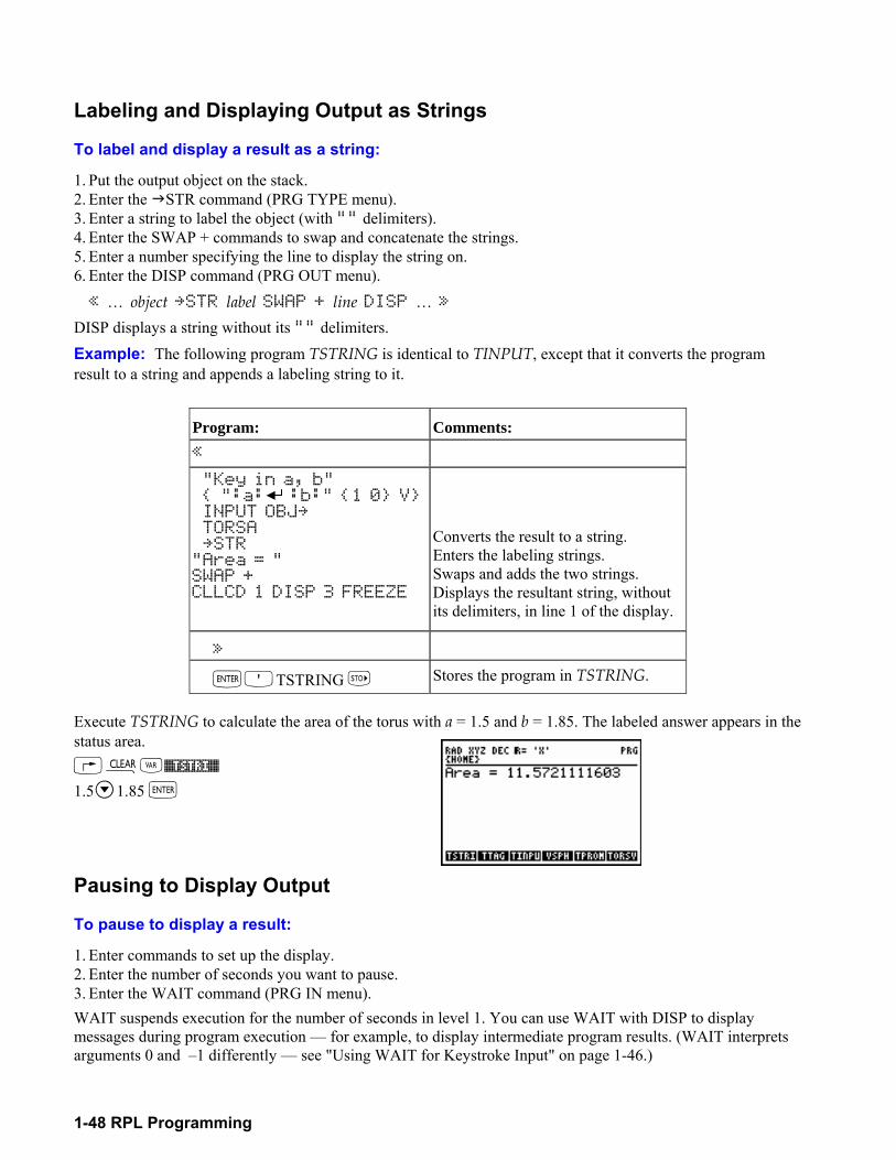
1-48 RPL Programming
Labeling and Displaying Output as Strings
To label and display a result as a string:
1. Put the output object on the stack. 2. Enter the "STR command (PRG TYPE menu). 3. Enter a string to label the object (with "" delimiters). 4. Enter the SWAP + commands to swap and concatenate the strings. 5. Enter a number specifying the line to display the string on. 6. Enter the DISP command (PRG OUT menu). « object STR label SWAP + line DISP »
DISP displays a string without its "" delimiters. Example: The following program TSTRING is identical to TINPUT, except that it converts the program result to a string and appends a labeling string to it.
Program: Comments: «
"Key in a, b" ":a: :b:" 1 0 V INPUT OBJ TORSA STR "Area = " SWAP + CLLCD 1 DISP 3 FREEZE
Converts the result to a string. Enters the labeling strings. Swaps and adds the two strings. Displays the resultant string, without its delimiters, in line 1 of the display.
»
`OTSTRING Stores the program in TSTRING.
Execute TSTRING to calculate the area of the torus with a = 1.5 and b = 1.85. The labeled answer appears in the status area. @·J%TSTRI%
1.5 1.85 `
Pausing to Display Output
To pause to display a result:
1. Enter commands to set up the display. 2. Enter the number of seconds you want to pause. 3. Enter the WAIT command (PRG IN menu). WAIT suspends execution for the number of seconds in level 1. You can use WAIT with DISP to display messages during program execution for example, to display intermediate program results. (WAIT interprets arguments 0 and 1 differently see "Using WAIT for Keystroke Input" on page 1-46.)
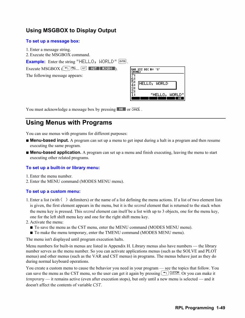
RPL Programming 1-49
Using MSGBOX to Display Output
To set up a message box:
1. Enter a message string. 2. Execute the MSGBOX command. Example: Enter the string "HELLO, WORLD" `. Execute MSGBOX (!°L %OUT% %MSGBO%). The following message appears:
You must acknowledge a message box by pressing %OK% or −.
Using Menus with Programs You can use menus with programs for different purposes: ! Menu-based input. A program can set up a menu to get input during a halt in a program and then resume
executing the same program. ! Menu-based application. A program can set up a menu and finish executing, leaving the menu to start
executing other related programs.
To set up a built-in or library menu:
1. Enter the menu number. 2. Enter the MENU command (MODES MENU menu).
To set up a custom menu:
1. Enter a list (with delimiters) or the name of a list defining the menu actions. If a list of two element lists is given, the first element appears in the menu, but it is the second element that is returned to the stack when the menu key is pressed. This second element can itself be a list with up to 3 objects, one for the menu key, one for the left shift menu key and one for the right shift menu key.
2. Activate the menu: ! To save the menu as the CST menu, enter the MENU command (MODES MENU menu). ! To make the menu temporary, enter the TMENU command (MODES MENU menu).
The menu isn't displayed until program execution halts. Menu numbers for built-in menus are listed in Appendix H. Library menus also have numbers the library number serves as the menu number. So you can activate applications menus (such as the SOLVE and PLOT menus) and other menus (such as the VAR and CST menus) in programs. The menus behave just as they do during normal keyboard operations. You create a custom menu to cause the behavior you need in your program see the topics that follow. You can save the menu as the CST menu, so the user can get it again by pressing !£. Or you can make it temporary it remains active (even after execution stops), but only until a new menu is selected and it doesn't affect the contents of variable CST.
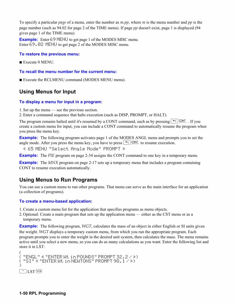
1-50 RPL Programming
To specify a particular page of a menu, enter the number as m.pp, where m is the menu number and pp is the page number (such as 94.02 for page 2 of the TIME menu). If page pp doesn't exist, page 1 is displayed (94 gives page 1 of the TIME menu). Example: Enter 69 MENU to get page 1 of the MODES MISC menu. Enter 69.02 MENU to get page 2 of the MODES MISC menu.
To restore the previous menu:
! Execute 0 MENU.
To recall the menu number for the current menu:
! Execute the RCLMENU command (MODES MENU menu). Using Menus for Input
To display a menu for input in a program:
1. Set up the menu see the previous section. 2. Enter a command sequence that halts execution (such as DISP, PROMPT, or HALT). The program remains halted until it's resumed by a CONT command, such as by pressing !æ. If you create a custom menu for input, you can include a CONT command to automatically resume the program when you press the menu key. Example: The following program activates page 1 of the MODES ANGL menu and prompts you to set the angle mode. After you press the menu key, you have to press !æto resume execution. « 65 MENU "Select Angle Mode" PROMPT »
Example: The PIE program on page 2-34 assigns the CONT command to one key in a temporary menu.
Example: The MNX program on page 2-17 sets up a temporary menu that includes a program containing CONT to resume execution automatically. Using Menus to Run Programs You can use a custom menu to run other programs. That menu can serve as the main interface for an application (a collection of programs).
To create a menu-based application:
1. Create a custom menu list for the application that specifies programs as menu objects. 2. Optional: Create a main program that sets up the application menu either as the CST menu or as a
temporary menu. Example: The following program, WGT, calculates the mass of an object in either English or SI units given the weight. WGT displays a temporary custom menu, from which you run the appropriate program. Each program prompts you to enter the weight in the desired unit system, then calculates the mass. The menu remains active until you select a new menu, so you can do as many calculations as you want. Enter the following list and store it in LST: "ENGL" « "ENTER Wt in POUNDS" PROMPT 32.2 / » "SI" « "ENTER Wt in NEWTONS" PROMPT 98.1 / »
OLST
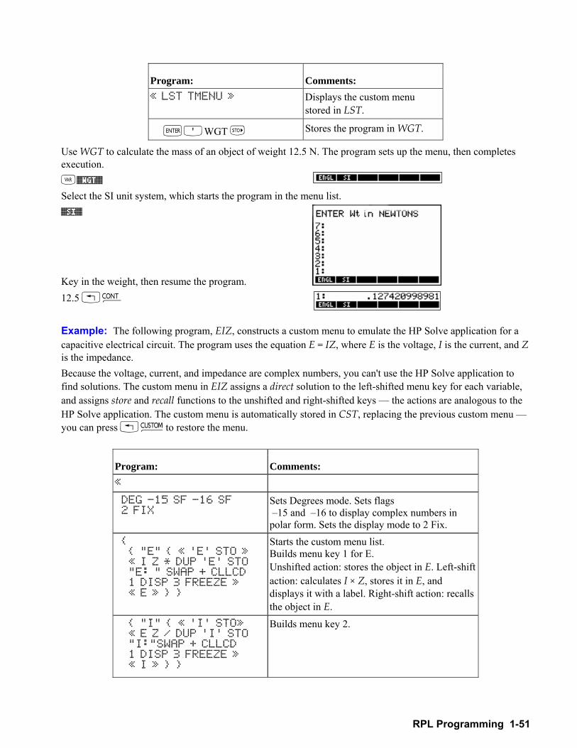
RPL Programming 1-51
Program: Comments: « LST TMENU » Displays the custom menu
stored in LST.
`OWGT Stores the program in WGT.
Use WGT to calculate the mass of an object of weight 12.5 N. The program sets up the menu, then completes execution. J%WGT%
Select the SI unit system, which starts the program in the menu list. %SI%
Key in the weight, then resume the program. 12.5 !æ Example: The following program, EIZ, constructs a custom menu to emulate the HP Solve application for a capacitive electrical circuit. The program uses the equation E = IZ, where E is the voltage, I is the current, and Z is the impedance. Because the voltage, current, and impedance are complex numbers, you can't use the HP Solve application to find solutions. The custom menu in EIZ assigns a direct solution to the left-shifted menu key for each variable, and assigns store and recall functions to the unshifted and right-shifted keys the actions are analogous to the HP Solve application. The custom menu is automatically stored in CST, replacing the previous custom menu you can press !£ to restore the menu.
Program: Comments: «
DEG -15 SF -16 SF 2 FIX
Sets Degrees mode. Sets flags 15 and 16 to display complex numbers in polar form. Sets the display mode to 2 Fix.
"E" « 'E' STO » « I Z * DUP 'E' STO "E: " SWAP + CLLCD 1 DISP 3 FREEZE » « E »
Starts the custom menu list. Builds menu key 1 for E. Unshifted action: stores the object in E. Left-shift action: calculates I × Z, stores it in E, and displays it with a label. Right-shift action: recalls the object in E.
"I" « 'I' STO» « E Z / DUP 'I' STO "I:"SWAP + CLLCD 1 DISP 3 FREEZE » « I »
Builds menu key 2.
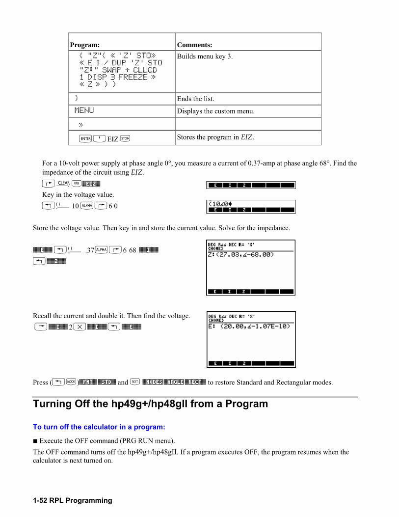
1-52 RPL Programming
Program: Comments: "Z" « 'Z' STO» « E I / DUP 'Z' STO "Z:" SWAP + CLLCD 1 DISP 3 FREEZE » « Z »
Builds menu key 3.
Ends the list.
MENU Displays the custom menu.
»
`OEIZ Stores the program in EIZ.
For a 10-volt power supply at phase angle 0°, you measure a current of 0.37-amp at phase angle 68°. Find the impedance of the circuit using EIZ.
@·J%EIZ% Key in the voltage value. !Ü10 ~@6 0
Store the voltage value. Then key in and store the current value. Solve for the impedance. %%E%% !Ü .37 ~@6 68 %%I%%
!%%Z%% Recall the current and double it. Then find the voltage. @%%I%% 2 *%%I%% !%%E%% Press (!H)%FMT% %STD% and L %MODES %ANGLE %RECT% to restore Standard and Rectangular modes.
Turning Off the hp49g+/hp48gII from a Program
To turn off the calculator in a program:
! Execute the OFF command (PRG RUN menu). The OFF command turns off the hp49g+/hp48gII. If a program executes OFF, the program resumes when the calculator is next turned on.
2
RPL Programming Examples 2-1
2.RPL Programming Examples The programs in this chapter demonstrate basic programming concepts. These programs are intended to improve your programming skills, and to provide supplementary functions for your calculator. At the end of each program, the program's checksum and size in bytes are listed to help make sure you typed the program in correctly. (The checksum is a binary integer that uniquely identifies the program based on its contents). To make sure you've keyed the program in correctly, store it in its name, put the name in level 1, then execute the BYTES command (!°#MEM# %BYTES%). This returns the program's checksum to level 2, and its size in bytes to level 1. (If you execute BYTES with the program object in level 1, you'll get a different byte count.) The examples in this chapter assume the hp49g+/hp48gII is in its initial, default condition they assume you haven't changed any of the hp49g+/hp48gII operating modes. (To reset the calculator to this condition, see Memory Reset in chapter 5 of the hp49g+/hp48gII User's Guide.) Each program listing in this chapter gives the following information: ! A brief description of the program. ! A syntax diagram (where needed) showing the program's required inputs and resulting outputs. ! Discussion of special programming techniques in the program. ! Any other programs needed. ! The program listing. ! The program's checksum and byte size.
Fibonacci Numbers This section includes three programs that calculate Fibonacci numbers: ! FIB1 is a user-defined function that is defined recursively (that is, its defining procedure contains its own
name). FIB1 is short.
! FIB2 is a user-defined function with a definite loop. It's longer and more complicated than FIB1, but faster.
! FIBT calls both FIB1 and FIB2 and calculates the execution time of each subprogram.
FIB1 and FIB2 demonstrate an approach to calculating the nth Fibonacci number Fn, where:
F0 = 0, F1 = 1, Fn = Fn-1 + Fn-2
FIB1 (Fibonacci Numbers, Recursive Version)
Level 1 " Level 1 n " Fn
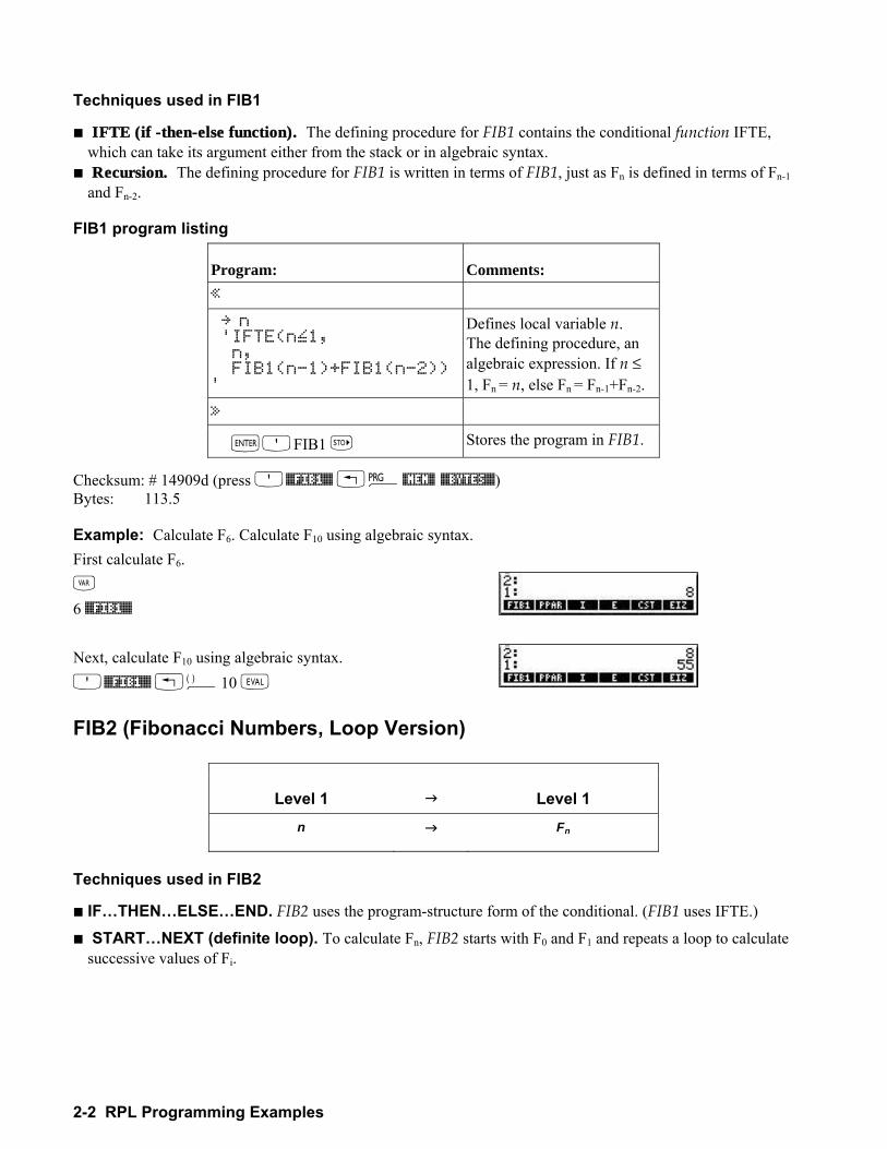
2-2 RPL Programming Examples
Techniques used in FIB1
! IFTE (if -then-else function). The defining procedure for FIB1 contains the conditional function IFTE, which can take its argument either from the stack or in algebraic syntax.
! Recursion. The defining procedure for FIB1 is written in terms of FIB1, just as Fn is defined in terms of Fn-1 and Fn-2.
FIB1 program listing
Program: Comments: « n 'IFTE(n‰1, n, FIB1(n-1)+FIB1(n-2))'
Defines local variable n. The defining procedure, an algebraic expression. If n ≤ 1, Fn = n, else Fn = Fn-1+Fn-2.
»
`OFIB1 K Stores the program in FIB1.
Checksum: # 14909d (press O%FIB1% !°#MEM# %BYTES%) Bytes: 113.5
Example: Calculate F6. Calculate F10 using algebraic syntax. First calculate F6. J
6 %FIB1%
Next, calculate F10 using algebraic syntax. O%FIB1% !Ü10 N FIB2 (Fibonacci Numbers, Loop Version)
Level 1 " Level 1 n " Fn
Techniques used in FIB2
! IFTHENELSEEND. FIB2 uses the program-structure form of the conditional. (FIB1 uses IFTE.)
! STARTNEXT (definite loop). To calculate Fn, FIB2 starts with F0 and F1 and repeats a loop to calculate successive values of Fi.
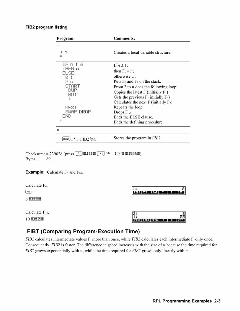
RPL Programming Examples 2-3
FIB2 program listing
Program: Comments: « n «
Creates a local variable structure.
IF n 1 ‰ THEN n ELSE 0 1 2 n START DUP ROT + NEXT SWAP DROP END »
If n ≤ 1, then Fn = n; otherwise Puts F0 and F1 on the stack. From 2 to n does the following loop: Copies the latest F (initially F1) Gets the previous F (initially F0) Calculates the next F (initially F2) Repeats the loop. Drops Fn-1. Ends the ELSE clause. Ends the defining procedure.
»
`O FIB2 K Stores the program in FIB2.
Checksum: # 23902d (press O%FIB2% !°#MEM# %BYTES%) Bytes: 89
Example: Calculate F6 and F10.
Calculate F6. J 6 %FIB2% Calculate F10. 10 %FIB2%
FIBT (Comparing Program-Execution Time) FIB1 calculates intermediate values Fi more than once, while FIB2 calculates each intermediate Fi only once. Consequently, FIB2 is faster. The difference in speed increases with the size of n because the time required for FIB1 grows exponentially with n, while the time required for FIB2 grows only linearly with n.
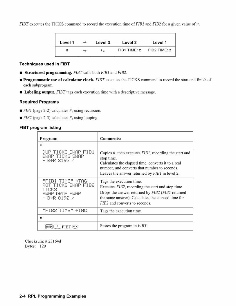
2-4 RPL Programming Examples
FIBT executes the TICKS command to record the execution time of FIB1 and FIB2 for a given value of n.
Level 1 " Level 3 Level 2 Level 1 n " Fn FIB1 TIME: z FIB2 TIME: z
Techniques used in FIBT
! Structured programming. FIBT calls both FIB1 and FIB2.
! Programmatic use of calculator clock. FIBT executes the TICKS command to record the start and finish of each subprogram.
! Labeling output. FIBT tags each execution time with a descriptive message.
Required Programs
! FIB1 (page 2-2) calculates Fn using recursion.
! FIB2 (page 2-3) calculates Fn using looping.
FIBT program listing
Program: Comments: « DUP TICKS SWAP FIB1 SWAP TICKS SWAP - BR 8192 /
Copies n, then executes FIB1, recording the start and stop time. Calculates the elapsed time, converts it to a real number, and converts that number to seconds. Leaves the answer returned by FIB1 in level 2.
"FIB1 TIME" TAG ROT TICKS SWAP FIB2 TICKS SWAP DROP SWAP - BR 8192 /
Tags the execution time. Executes FIB2, recording the start and stop time. Drops the answer returned by FIB2 (FIB1 returned the same answer). Calculates the elapsed time for FIB2 and converts to seconds.
"FIB2 TIME" TAG Tags the execution time. »
`OFIBT K Stores the program in FIBT.
Checksum: # 23164d Bytes: 129
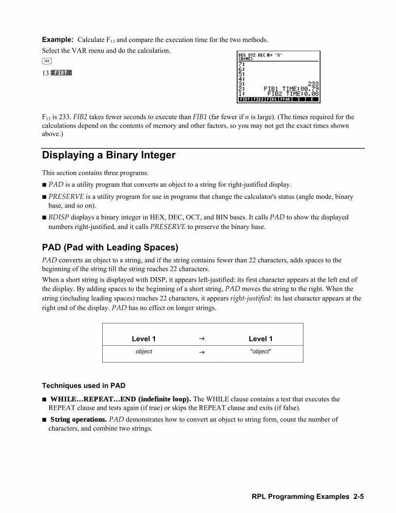
RPL Programming Examples 2-5
Example: Calculate F13 and compare the execution time for the two methods. Select the VAR menu and do the calculation. J 13 %FIBT%
F13 is 233. FIB2 takes fewer seconds to execute than FIB1 (far fewer if n is large). (The times required for the calculations depend on the contents of memory and other factors, so you may not get the exact times shown above.)
Displaying a Binary Integer This section contains three programs: ! PAD is a utility program that converts an object to a string for right-justified display.
! PRESERVE is a utility program for use in programs that change the calculator's status (angle mode, binary base, and so on).
! BDISP displays a binary integer in HEX, DEC, OCT, and BIN bases. It calls PAD to show the displayed numbers right-justified, and it calls PRESERVE to preserve the binary base.
PAD (Pad with Leading Spaces) PAD converts an object to a string, and if the string contains fewer than 22 characters, adds spaces to the beginning of the string till the string reaches 22 characters. When a short string is displayed with DISP, it appears left-justified: its first character appears at the left end of the display. By adding spaces to the beginning of a short string, PAD moves the string to the right. When the string (including leading spaces) reaches 22 characters, it appears right-justified: its last character appears at the right end of the display. PAD has no effect on longer strings.
Level 1 " Level 1 object " "object"
Techniques used in PAD
! WHILE…REPEAT…END (indefinite loop). The WHILE clause contains a test that executes the REPEAT clause and tests again (if true) or skips the REPEAT clause and exits (if false).
! String operations. PAD demonstrates how to convert an object to string form, count the number of characters, and combine two strings.
2-6 RPL Programming Examples
PAD program listing
Program: Comments: « STR Makes sure the object is in string form. (Strings
are unaffected by this command.) WHILE DUP SIZE 22 < REPEAT " " SWAP +
Repeats if the string contains fewer than 22 characters. Loop-clause adds a leading space.
END End loop. »
`OPAD K Stores the program in PAD.
Checksum: # 6577d Bytes: 57.5 PAD is demonstrated in the program BDISP. PRESERVE (Save and Restore Previous Status) PRESERVE stores the current calculator (flag) status, executes a program from the stack, and restores the previous status.
Level 1 " Level 1 «program» " result of program
'program' " result of program
Techniques used in PRESERVE
! Preserving calculator flag status. PRESERVE uses RCLF (recall flags) to record the current status of the calculator in a binary integer, and STOF (store flags) to restore the status from that binary integer.
! Local-variable structure. PRESERVE creates a local variable structure to briefly remove the binary integer from the stack. Its defining procedure simply evaluates the program argument, then puts the binary integer back on the stack and executes STOF.
! Error trapping. PRESERVE uses IFERR to trap faulty program execution on the stack and to restore flags. DOERR shows the error if one occurs.
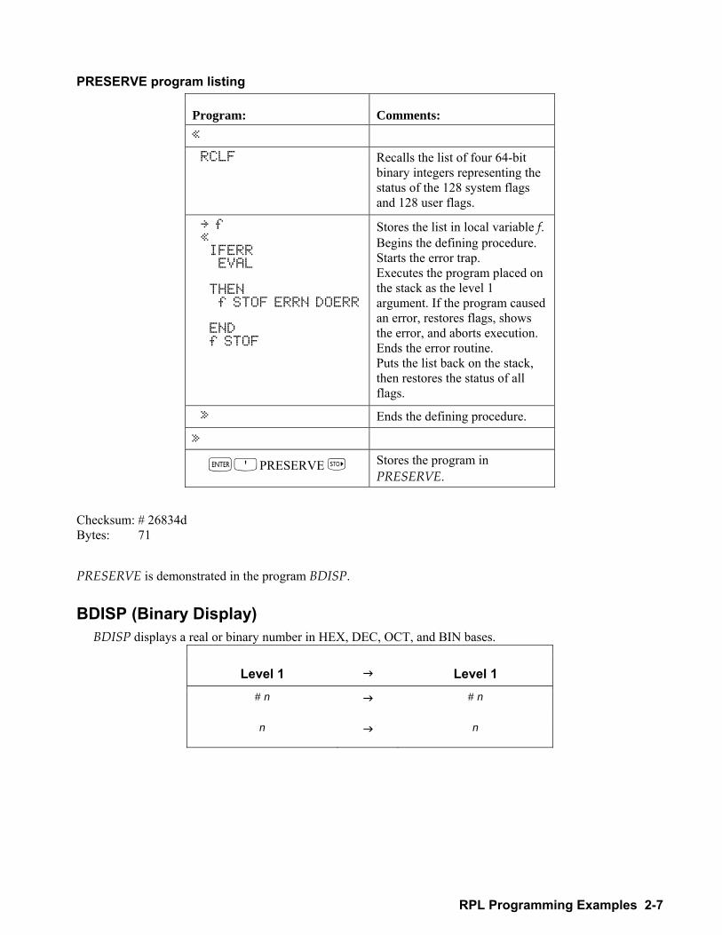
RPL Programming Examples 2-7
PRESERVE program listing
Program: Comments: « RCLF Recalls the list of four 64-bit
binary integers representing the status of the 128 system flags and 128 user flags.
f « IFERR EVAL THEN f STOF ERRN DOERR END f STOF
Stores the list in local variable f. Begins the defining procedure. Starts the error trap. Executes the program placed on the stack as the level 1 argument. If the program caused an error, restores flags, shows the error, and aborts execution. Ends the error routine. Puts the list back on the stack, then restores the status of all flags.
» Ends the defining procedure. »
`OPRESERVE K Stores the program in PRESERVE.
Checksum: # 26834d Bytes: 71 PRESERVE is demonstrated in the program BDISP. BDISP (Binary Display)
BDISP displays a real or binary number in HEX, DEC, OCT, and BIN bases.
Level 1 " Level 1 # n " # n
n " n
2-8 RPL Programming Examples
Techniques used in BDISP
! IFERR…THEN…END (error trap). To accommodate real-number arguments, BDISP includes the command R"B (real-to-binary). However, this command causes an error if the argument is already a binary integer. To maintain execution if an error occurs, the R"B command is placed inside an IFERR clause. No action is required when an error occurs (since a binary number is an acceptable argument), so the THEN clause contains no commands.
! Enabling LASTARG. In case an error occurs, the LASTARG recovery feature must be enabled to return the argument (the binary number) to the stack. BDISP clears flag 55 to enable this.
! FOR…NEXT loop (definite loop with counter). BDISP executes a loop from 1 to 4, each time displaying n (the number) in a different base on a different line. The loop counter (named j in this program) is a local variable created by the FORNEXT program structure (rather than by a command), and automatically incremented by NEXT.
! Unnamed programs as arguments. A program defined only by its « and » delimiters (not stored in a variable) is not automatically evaluated, but is placed on the stack and can be used as an argument for a subroutine. BDISP demonstrates two uses for unnamed program arguments:
" BDISP contains a main program argument and a call to PRESERVE. This program argument goes on the stack and is executed by PRESERVE.
" BDISP also contains four program arguments that customize the action of the loop. Each of these contains a command to change the binary base, and each iteration of the loop evaluates one of these arguments.
When BDISP creates a local variable for n, the defining procedure is an unnamed program. However, since this program is a defining procedure for a local variable structure, it is automatically executed.
Required Programs PAD ! PAD (Pad with Leading Spaces) expands a string to 22 characters so that DISP shows it right-justified. PRESERVE PRESERVE (S) stores the current status, executes the main nested program, and restores the status.
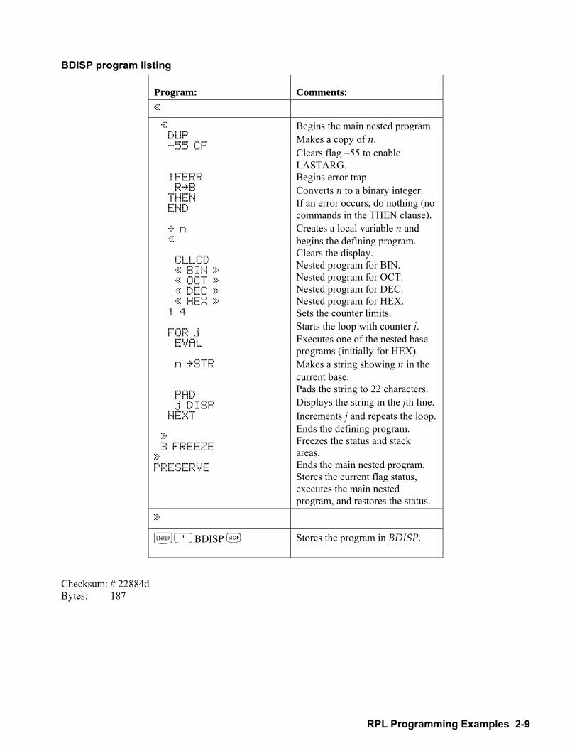
RPL Programming Examples 2-9
BDISP program listing
Program: Comments: « « DUP -55 CF IFERR RB THEN END n « CLLCD « BIN » « OCT » « DEC » « HEX » 1 4 FOR j EVAL n STR PAD j DISP NEXT » 3 FREEZE » PRESERVE
Begins the main nested program. Makes a copy of n. Clears flag 55 to enable LASTARG. Begins error trap. Converts n to a binary integer. If an error occurs, do nothing (no commands in the THEN clause). Creates a local variable n and begins the defining program. Clears the display. Nested program for BIN. Nested program for OCT. Nested program for DEC. Nested program for HEX. Sets the counter limits. Starts the loop with counter j. Executes one of the nested base programs (initially for HEX). Makes a string showing n in the current base. Pads the string to 22 characters. Displays the string in the jth line. Increments j and repeats the loop. Ends the defining program. Freezes the status and stack areas. Ends the main nested program. Stores the current flag status, executes the main nested program, and restores the status.
»
`OBDISP K Stores the program in BDISP.
Checksum: # 22884d Bytes: 187
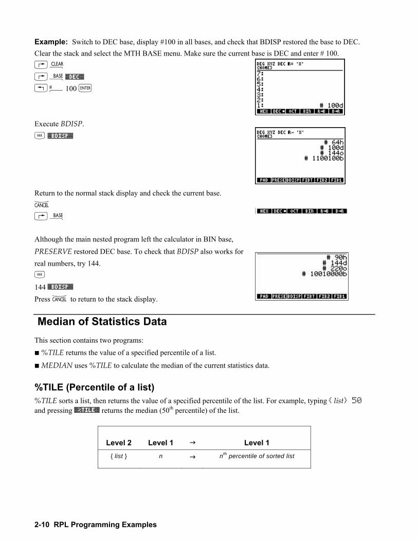
2-10 RPL Programming Examples
Example: Switch to DEC base, display #100 in all bases, and check that BDISP restored the base to DEC. Clear the stack and select the MTH BASE menu. Make sure the current base is DEC and enter # 100. · ã%DEC%
!â100 ` Execute BDISP.
J %BDISP% Return to the normal stack display and check the current base. − ã Although the main nested program left the calculator in BIN base, PRESERVE restored DEC base. To check that BDISP also works for real numbers, try 144. J 144 %BDISP%
Press − to return to the stack display.
Median of Statistics Data This section contains two programs: ! %TILE returns the value of a specified percentile of a list.
! MEDIAN uses %TILE to calculate the median of the current statistics data. %TILE (Percentile of a list) %TILE sorts a list, then returns the value of a specified percentile of the list. For example, typing list 50 and pressing %©TILE% returns the median (50th percentile) of the list.
Level 2 Level 1 " Level 1 list n " nth percentile of sorted list
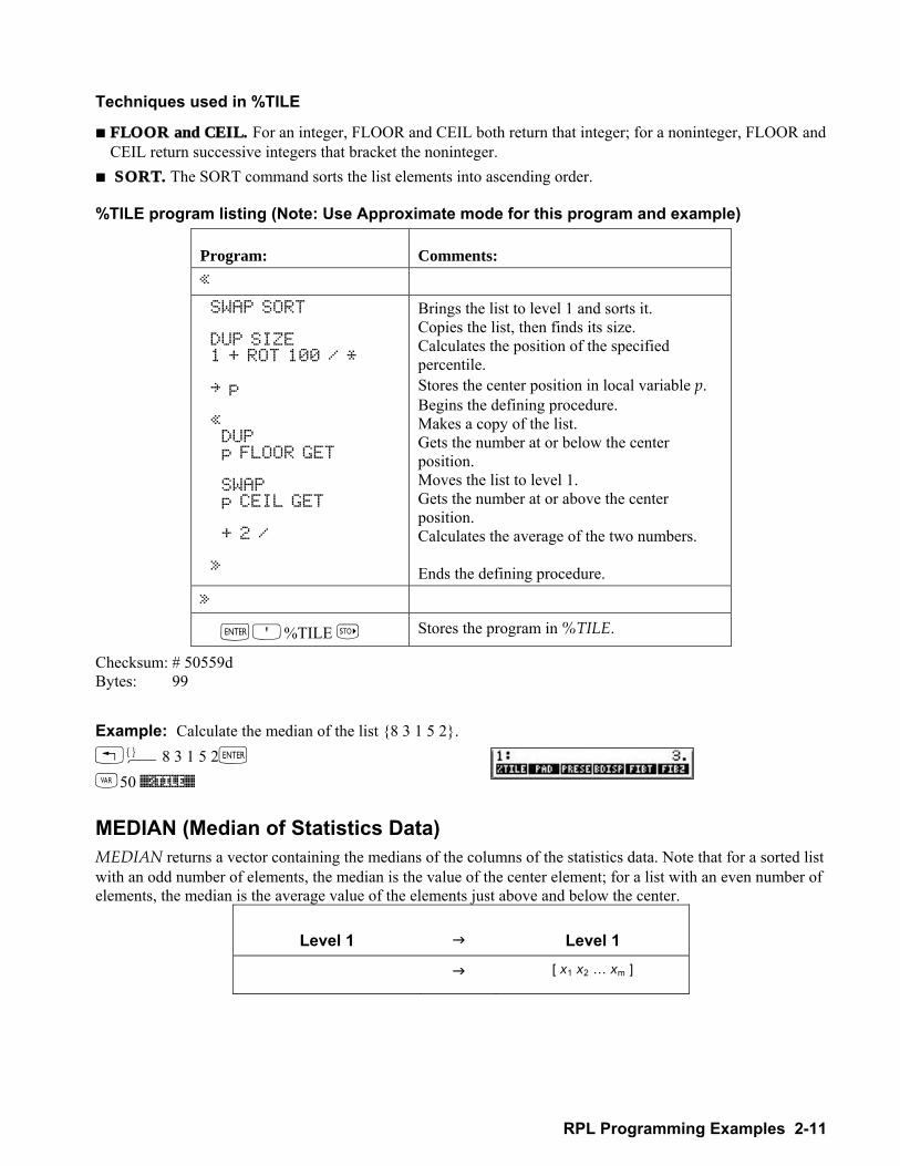
RPL Programming Examples 2-11
Techniques used in %TILE
! FLOOR and CEIL. For an integer, FLOOR and CEIL both return that integer; for a noninteger, FLOOR and CEIL return successive integers that bracket the noninteger.
! SORT. The SORT command sorts the list elements into ascending order.
%TILE program listing (Note: Use Approximate mode for this program and example)
Program: Comments: « SWAP SORT DUP SIZE 1 + ROT 100 / * p « DUP p FLOOR GET SWAP p CEIL GET + 2 / »
Brings the list to level 1 and sorts it. Copies the list, then finds its size. Calculates the position of the specified percentile. Stores the center position in local variable p. Begins the defining procedure. Makes a copy of the list. Gets the number at or below the center position. Moves the list to level 1. Gets the number at or above the center position. Calculates the average of the two numbers. Ends the defining procedure.
»
`O%TILE K Stores the program in %TILE.
Checksum: # 50559d Bytes: 99
Example: Calculate the median of the list 8 3 1 5 2. !ä8 3 1 5 2` J50 %©TILE% MEDIAN (Median of Statistics Data) MEDIAN returns a vector containing the medians of the columns of the statistics data. Note that for a sorted list with an odd number of elements, the median is the value of the center element; for a list with an even number of elements, the median is the average value of the elements just above and below the center.
Level 1 " Level 1 " [ x1 x2 xm ]
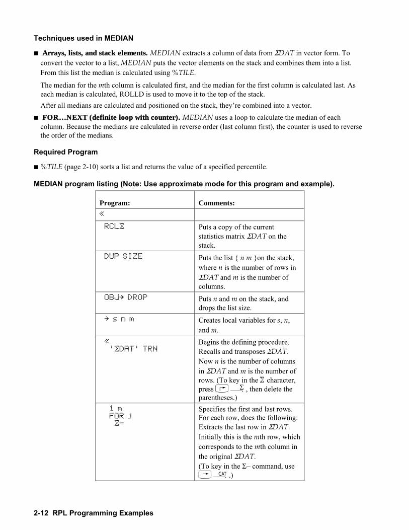
2-12 RPL Programming Examples
Techniques used in MEDIAN
! Arrays, lists, and stack elements. MEDIAN extracts a column of data from ΣDAT in vector form. To convert the vector to a list, MEDIAN puts the vector elements on the stack and combines them into a list. From this list the median is calculated using %TILE.
The median for the mth column is calculated first, and the median for the first column is calculated last. As each median is calculated, ROLLD is used to move it to the top of the stack. After all medians are calculated and positioned on the stack, theyre combined into a vector.
! FOR…NEXT (definite loop with counter). MEDIAN uses a loop to calculate the median of each column. Because the medians are calculated in reverse order (last column first), the counter is used to reverse the order of the medians.
Required Program
! %TILE (page 2-10) sorts a list and returns the value of a specified percentile.
MEDIAN program listing (Note: Use approximate mode for this program and example).
Program: Comments: « RCL…
Puts a copy of the current statistics matrix ΣDAT on the stack.
DUP SIZE Puts the list n m on the stack, where n is the number of rows in ΣDAT and m is the number of columns.
OBJ DROP Puts n and m on the stack, and drops the list size.
s n m Creates local variables for s, n, and m.
« '…DAT' TRN
Begins the defining procedure. Recalls and transposes ΣDAT. Now n is the number of columns in ΣDAT and m is the number of rows. (To key in the … character, press @½, then delete the parentheses.)
1 m FOR j …-
Specifies the first and last rows. For each row, does the following: Extracts the last row in ΣDAT. Initially this is the mth row, which corresponds to the mth column in the original ΣDAT. (To key in the Σ command, use @µ.)
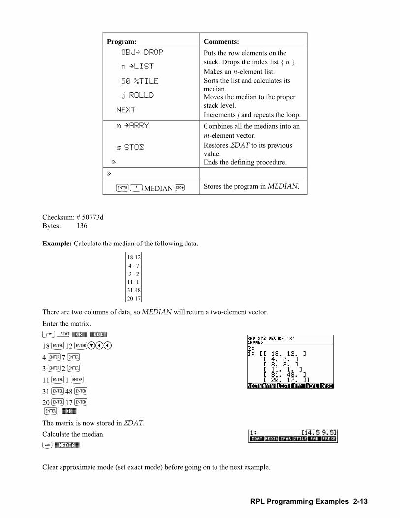
RPL Programming Examples 2-13
Program: Comments: OBJ DROP n LIST 50 %TILE j ROLLD NEXT
Puts the row elements on the stack. Drops the index list n . Makes an n-element list. Sorts the list and calculates its median. Moves the median to the proper stack level. Increments j and repeats the loop.
m ARRY s STO… »
Combines all the medians into an m-element vector. Restores ΣDAT to its previous value. Ends the defining procedure.
»
`OMEDIAN K Stores the program in MEDIAN.
Checksum: # 50773d Bytes: 136
Example: Calculate the median of the following data.
18 124 73 211 131 4820 17
There are two columns of data, so MEDIAN will return a two-element vector. Enter the matrix. Ù%OK% %EDIT 18 `12 ` 4 `7 ` 3 `2 ` 11 `1 ` 31 `48 ` 20 `17 ` ` %OK% The matrix is now stored in ΣDAT. Calculate the median. J %MEDIA%
Clear approximate mode (set exact mode) before going on to the next example.
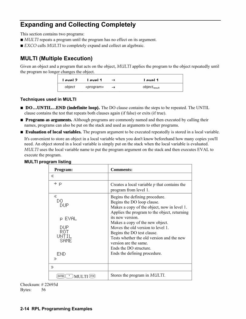
2-14 RPL Programming Examples
Expanding and Collecting Completely This section contains two programs: ! MULTI repeats a program until the program has no effect on its argument. ! EXCO calls MULTI to completely expand and collect an algebraic. MULTI (Multiple Execution) Given an object and a program that acts on the object, MULTI applies the program to the object repeatedly until the program no longer changes the object.
Level 2 Level 1 " Level 1object «program» " objectresult
Techniques used in MULTI
! DO…UNTIL…END (indefinite loop). The DO clause contains the steps to be repeated. The UNTIL clause contains the test that repeats both clauses again (if false) or exits (if true).
! Programs as arguments. Although programs are commonly named and then executed by calling their names, programs can also be put on the stack and used as arguments to other programs.
! Evaluation of local variables. The program argument to be executed repeatedly is stored in a local variable. It's convenient to store an object in a local variable when you don't know beforehand how many copies you'll need. An object stored in a local variable is simply put on the stack when the local variable is evaluated. MULTI uses the local variable name to put the program argument on the stack and then executes EVAL to execute the program. MULTI program listing
Program: Comments: « p Creates a local variable p that contains the
program from level 1. « DO DUP p EVAL DUP ROT UNTIL SAME END »
Begins the defining procedure. Begins the DO loop clause. Makes a copy of the object, now in level 1. Applies the program to the object, returning its new version. Makes a copy of the new object. Moves the old version to level 1. Begins the DO test clause. Tests whether the old version and the new version are the same. Ends the DO structure. Ends the defining procedure.
»
`OMULTI K Stores the program in MULTI.
Checksum: # 22693d Bytes: 56
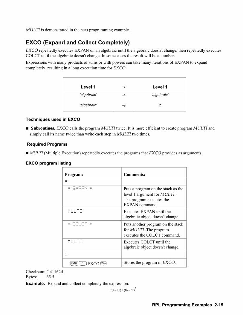
RPL Programming Examples 2-15
MULTI is demonstrated in the next programming example. EXCO (Expand and Collect Completely) EXCO repeatedly executes EXPAN on an algebraic until the algebraic doesn't change, then repeatedly executes COLCT until the algebraic doesn't change. In some cases the result will be a number. Expressions with many products of sums or with powers can take many iterations of EXPAN to expand completely, resulting in a long execution time for EXCO.
Level 1 " Level 1 'algebraic' " 'algebraic'
'algebraic' " z
Techniques used in EXCO
! Subroutines. EXCO calls the program MULTI twice. It is more efficient to create program MULTI and simply call its name twice than write each step in MULTI two times.
Required Programs
! MULTI (Multiple Execution) repeatedly executes the programs that EXCO provides as arguments.
EXCO program listing
Program: Comments: « « EXPAN » Puts a program on the stack as the
level 1 argument for MULTI. The program executes the EXPAN command.
MULTI Executes EXPAN until the algebraic object doesn't change.
« COLCT » Puts another program on the stack for MULTI. The program executes the COLCT command.
MULTI Executes COLCT until the algebraic object doesn't change.
»
`OEXCO K Stores the program in EXCO.
Checksum: # 41162d Bytes: 65.5 Example: Expand and collect completely the expression: 3x 4y z+( ) 8x 5z( )2+
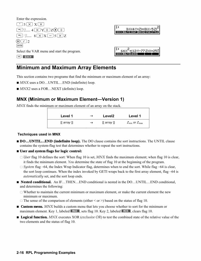
2-16 RPL Programming Examples
Enter the expression. O3 * X * !Ü4 *Y+Z + ! Ü 8 *X -5 *Z Q2 ` Select the VAR menu and start the program. J %EXCO%
Minimum and Maximum Array Elements This section contains two programs that find the minimum or maximum element of an array: ! MNX uses a DOUNTILEND (indefinite) loop.
! MNX2 uses a FORNEXT (definite) loop. MNX (Minimum or Maximum ElementVersion 1) MNX finds the minimum or maximum element of an array on the stack.
Level 1 " Level2 Level 1 [[ array ]] " [[ array ]] Zmin or Zmax
Techniques used in MNX
! DO…UNTIL…END (indefinite loop). The DO clause contains the sort instructions. The UNTIL clause contains the system-flag test that determines whether to repeat the sort instructions.
! User and system flags for logic control: " User flag 10 defines the sort: When flag 10 is set, MNX finds the maximum element; when flag 10 is clear,
it finds the minimum element. You determine the state of flag 10 at the beginning of the program. " System flag 64, the Index Wrap Indicator flag, determines when to end the sort. While flag 64 is clear,
the sort loop continues. When the index invoked by GETI wraps back to the first array element, flag 64 is automatically set, and the sort loop ends.
! Nested conditional. An IFTHENEND conditional is nested in the DOUNTILEND conditional, and determines the following: " Whether to maintain the current minimum or maximum element, or make the current element the new
minimum or maximum. " The sense of the comparison of elements (either < or >) based on the status of flag 10.
! Custom menu. MNX builds a custom menu that lets you choose whether to sort for the minimum or maximum element. Key 1, labeled %MAX%, sets flag 10. Key 2, labeled %MIN%, clears flag 10.
! Logical function. MNX executes XOR (exclusive OR) to test the combined state of the relative value of the two elements and the status of flag 10.
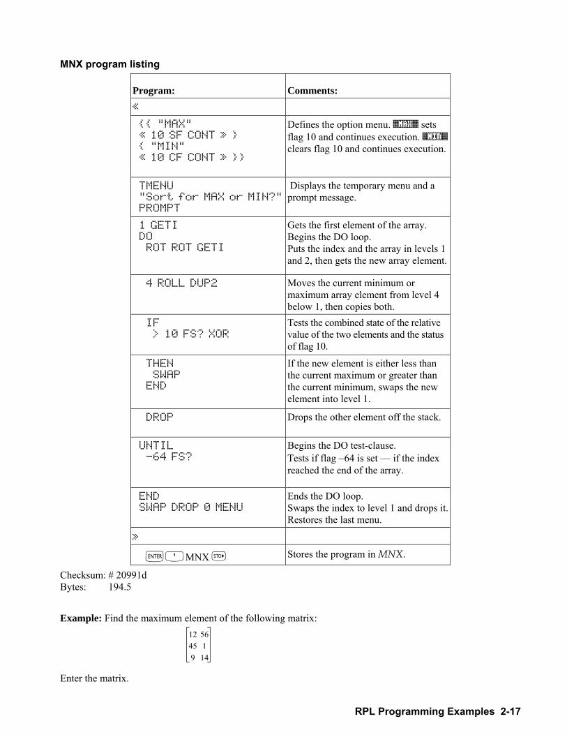
RPL Programming Examples 2-17
MNX program listing
Program: Comments: «
"MAX" « 10 SF CONT » "MIN" « 10 CF CONT »
Defines the option menu. %MAX% sets flag 10 and continues execution. %MIN% clears flag 10 and continues execution.
TMENU "Sort for MAX or MIN?" PROMPT
Displays the temporary menu and a prompt message.
1 GETI DO ROT ROT GETI
Gets the first element of the array. Begins the DO loop. Puts the index and the array in levels 1 and 2, then gets the new array element.
4 ROLL DUP2 Moves the current minimum or maximum array element from level 4 below 1, then copies both.
IF > 10 FS? XOR
Tests the combined state of the relative value of the two elements and the status of flag 10.
THEN SWAP END
If the new element is either less than the current maximum or greater than the current minimum, swaps the new element into level 1.
DROP Drops the other element off the stack.
UNTIL -64 FS?
Begins the DO test-clause. Tests if flag 64 is set if the index reached the end of the array.
END SWAP DROP 0 MENU
Ends the DO loop. Swaps the index to level 1 and drops it. Restores the last menu.
»
`OMNX K Stores the program in MNX.
Checksum: # 20991d Bytes: 194.5
Example: Find the maximum element of the following matrix:
12 5645 19 14
Enter the matrix.
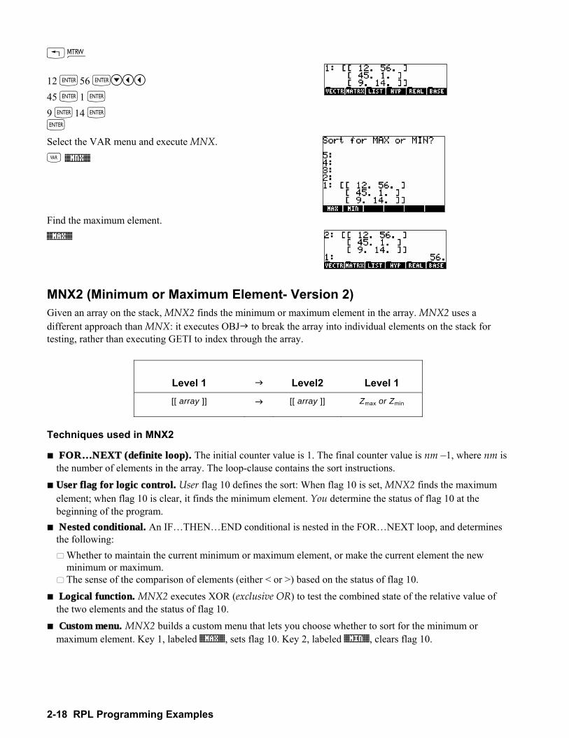
2-18 RPL Programming Examples
!² 12 `56 ` 45 `1 ` 9 `14 ` ` Select the VAR menu and execute MNX.
J %MNX% Find the maximum element. %MAX%
MNX2 (Minimum or Maximum Element- Version 2) Given an array on the stack, MNX2 finds the minimum or maximum element in the array. MNX2 uses a different approach than MNX: it executes OBJ" to break the array into individual elements on the stack for testing, rather than executing GETI to index through the array.
Level 1 " Level2 Level 1 [[ array ]] " [[ array ]] Zmax or Zmin
Techniques used in MNX2
! FOR…NEXT (definite loop). The initial counter value is 1. The final counter value is nm 1, where nm is the number of elements in the array. The loop-clause contains the sort instructions.
! User flag for logic control. User flag 10 defines the sort: When flag 10 is set, MNX2 finds the maximum element; when flag 10 is clear, it finds the minimum element. You determine the status of flag 10 at the beginning of the program.
! Nested conditional. An IFTHENEND conditional is nested in the FORNEXT loop, and determines the following: " Whether to maintain the current minimum or maximum element, or make the current element the new
minimum or maximum. " The sense of the comparison of elements (either < or >) based on the status of flag 10.
! Logical function. MNX2 executes XOR (exclusive OR) to test the combined state of the relative value of the two elements and the status of flag 10.
! Custom menu. MNX2 builds a custom menu that lets you choose whether to sort for the minimum or maximum element. Key 1, labeled %MAX%, sets flag 10. Key 2, labeled %MIN%, clears flag 10.
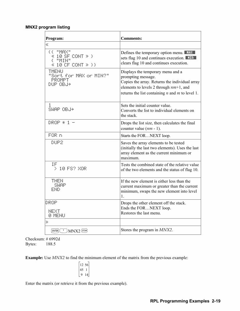
RPL Programming Examples 2-19
MNX2 program listing
Program: Comments: « "MAX" « 10 SF CONT » "MIN" « 10 CF CONT »
Defines the temporary option menu. %MAX% sets flag 10 and continues execution. %MIN% clears flag 10 and continues execution.
TMENU "Sort for MAX or MIN?" PROMPT DUP OBJ
Displays the temporary menu and a prompting message. Copies the array. Returns the individual array elements to levels 2 through nm+1, and returns the list containing n and m to level 1.
1 SWAP OBJ
Sets the initial counter value. Converts the list to individual elements on the stack.
DROP * 1 - Drops the list size, then calculates the final counter value (nm - 1).
FOR n Starts the FORNEXT loop. DUP2 Saves the array elements to be tested
(initially the last two elements). Uses the last array element as the current minimum or maximum.
IF > 10 FS? XOR
Tests the combined state of the relative value of the two elements and the status of flag 10.
THEN SWAP END
If the new element is either less than the current maximum or greater than the current minimum, swaps the new element into level 1.
DROP NEXT 0 MENU
Drops the other element off the stack. Ends the FORNEXT loop. Restores the last menu.
»
`OMNX2 K Stores the program in MNX2.
Checksum: # 6992d Bytes: 188.5 Example: Use MNX2 to find the minimum element of the matrix from the previous example:
12 5645 19 14
Enter the matrix (or retrieve it from the previous example).
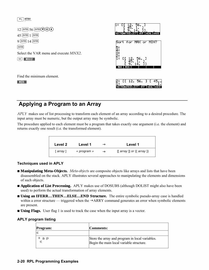
2-20 RPL Programming Examples
!² 12 `56 ` 45 `1 ` 9 `14 ` ` Select the VAR menu and execute MNX2.
J %MNX2% Find the minimum element. %MIN%
Applying a Program to an Array APLY makes use of list processing to transform each element of an array according to a desired procedure. The input array must be numeric, but the output array may be symbolic. The procedure applied to each element must be a program that takes exactly one argument (i.e. the element) and returns exactly one result (i.e. the transformed element).
Level 2 Level 1 " Level 1 [ array ] « program » " [[ array ]] or array
Techniques used in APLY
! Manipulating Meta-Objects. Meta-objects are composite objects like arrays and lists that have been disassembled on the stack. APLY illustrates several approaches to manipulating the elements and dimensions of such objects.
! Application of List Processing. APLY makes use of DOSUBS (although DOLIST might also have been used) to perform the actual transformation of array elements.
! Using an IFERR…THEN…ELSE…END Structure. The entire symbolic pseudo-array case is handled within a error structure triggered when the "ARRY command generates an error when symbolic elements are present.
! Using Flags. User flag 1 is used to track the case when the input array is a vector.
APLY program listing
Program: Comments: « a p «
Store the array and program in local variables. Begin the main local variable structure.
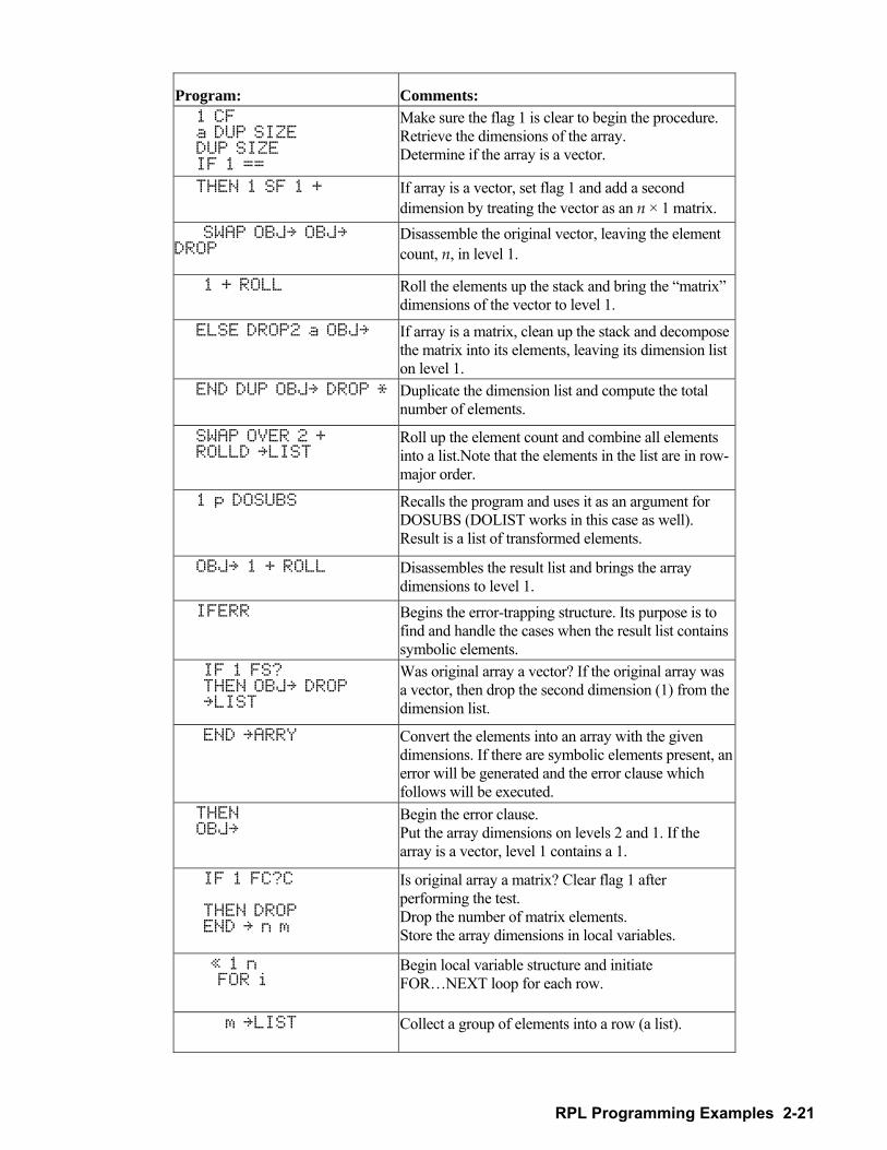
RPL Programming Examples 2-21
Program: Comments: 1 CF a DUP SIZE DUP SIZE IF 1 ==
Make sure the flag 1 is clear to begin the procedure. Retrieve the dimensions of the array. Determine if the array is a vector.
THEN 1 SF 1 + If array is a vector, set flag 1 and add a second dimension by treating the vector as an n × 1 matrix.
SWAP OBJ OBJ DROP
Disassemble the original vector, leaving the element count, n, in level 1.
1 + ROLL Roll the elements up the stack and bring the matrix dimensions of the vector to level 1.
ELSE DROP2 a OBJ If array is a matrix, clean up the stack and decompose the matrix into its elements, leaving its dimension list on level 1.
END DUP OBJ DROP * Duplicate the dimension list and compute the total number of elements.
SWAP OVER 2 + ROLLD LIST
Roll up the element count and combine all elements into a list.Note that the elements in the list are in row-major order.
1 p DOSUBS Recalls the program and uses it as an argument for DOSUBS (DOLIST works in this case as well). Result is a list of transformed elements.
OBJ 1 + ROLL Disassembles the result list and brings the array dimensions to level 1.
IFERR Begins the error-trapping structure. Its purpose is to find and handle the cases when the result list contains symbolic elements.
IF 1 FS? THEN OBJ DROP LIST
Was original array a vector? If the original array was a vector, then drop the second dimension (1) from the dimension list.
END ARRY Convert the elements into an array with the given dimensions. If there are symbolic elements present, an error will be generated and the error clause which follows will be executed.
THEN OBJ
Begin the error clause. Put the array dimensions on levels 2 and 1. If the array is a vector, level 1 contains a 1.
IF 1 FC?C THEN DROP END n m
Is original array a matrix? Clear flag 1 after performing the test. Drop the number of matrix elements. Store the array dimensions in local variables.
« 1 n FOR i
Begin local variable structure and initiate FORNEXT loop for each row.
m LIST Collect a group of elements into a row (a list).
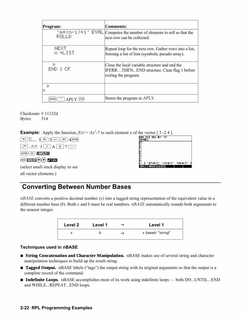
2-22 RPL Programming Examples
Program: Comments: 'm*(n-i)+i' EVAL ROLLD
Computes the number of elements to roll so that the next row can be collected.
NEXT n LIST
Repeat loop for the next row. Gather rows into a list, forming a list of lists (symbolic pseudo-array).
» END 1 CF
Close the local variable structure and end the IFERRTHEN...END structure. Clear flag 1 before exiting the program.
» »
`OAPLY K Stores the program in APLY.
Checksum: # 11132d Bytes: 314
Example: Apply the function, f(x) = Ax3-7 to each element x of the vector [ 3 -2 4 ]. !Ô32W4`
å 3 QA *7 -
`J %APLY% H#DISP
(select small stack display to see all vector elements.)
Converting Between Number Bases nBASE converts a positive decimal number (x) into a tagged string representation of the equivalent value in a different number base (b). Both x and b must be real numbers. nBASE automatically rounds both arguments to the nearest integer.
Level 2 Level 1 " Level 1 x b " x baseb: "string"
Techniques used in nBASE
! String Concatenation and Character Manipulation. nBASE makes use of several string and character manipulation techniques to build up the result string.
! Tagged Output. nBASE labels (tags) the output string with its original arguments so that the output is a complete record of the command.
! Indefinite Loops. nBASE accomplishes most of its work using indefinite loops both DO...UNTIL...END and WHILE...REPEAT...END loops.
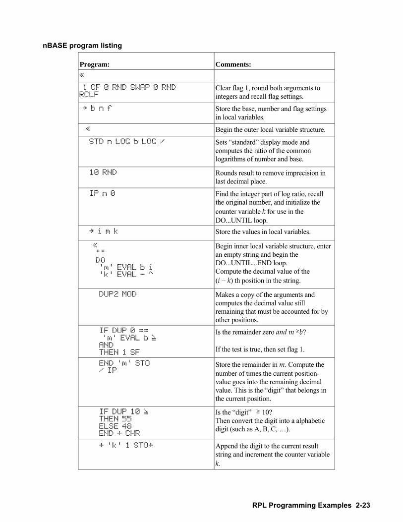
RPL Programming Examples 2-23
nBASE program listing
Program: Comments: « 1 CF 0 RND SWAP 0 RND RCLF
Clear flag 1, round both arguments to integers and recall flag settings.
b n f Store the base, number and flag settings in local variables.
« Begin the outer local variable structure.
STD n LOG b LOG / Sets standard display mode and computes the ratio of the common logarithms of number and base.
10 RND Rounds result to remove imprecision in last decimal place.
IP n 0 Find the integer part of log ratio, recall the original number, and initialize the counter variable k for use in the DO...UNTIL loop.
i m k Store the values in local variables.
« "" DO 'm' EVAL b i 'k' EVAL - ^
Begin inner local variable structure, enter an empty string and begin the DO...UNTIL...END loop. Compute the decimal value of the (i k) th position in the string.
DUP2 MOD Makes a copy of the arguments and computes the decimal value still remaining that must be accounted for by other positions.
IF DUP 0 == 'm' EVAL b Š AND THEN 1 SF
Is the remainder zero and m ≥b? If the test is true, then set flag 1.
END 'm' STO / IP
Store the remainder in m. Compute the number of times the current position-value goes into the remaining decimal value. This is the digit that belongs in the current position.
IF DUP 10 Š THEN 55 ELSE 48 END + CHR
Is the digit ≥ 10? Then convert the digit into a alphabetic digit (such as A, B, C, ).
+ 'k' 1 STO+ Append the digit to the current result string and increment the counter variable k.
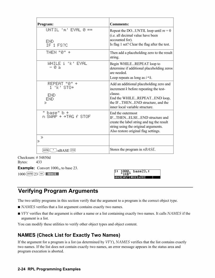
2-24 RPL Programming Examples
Program: Comments: UNTIL 'm' EVAL 0 == END IF 1 FS?C
Repeat the DO...UNTIL loop until m = 0 (i.e. all decimal value have been accounted for). Is flag 1 set? Clear the flag after the test.
THEN "0" + Then add a placeholding zero to the result string.
WHILE i 'k' EVAL - 0 Š
Begin WHILE...REPEAT loop to determine if additional placeholding zeros are needed. Loop repeats as long as i ≠ k.
REPEAT "0" + 1 'k' STO+ END END »
Add an additional placeholding zero and increment k before repeating the test-clause. End the WHILE...REPEAT...END loop, the IF...THEN...END structure, and the inner local variable structure.
" base" b + n SWAP + TAG f STOF
End the outermost IF...THEN...ELSE...END structure and create the label string and tag the result string using the original arguments. Also restore original flag settings.
» »
`OnBASE K Stores the program in nBASE.
Checksum: # 54850d Bytes: 433 Example: Convert 100010 to base 23. 1000 `23 J %NBASE%
Verifying Program Arguments The two utility programs in this section verify that the argument to a program is the correct object type. ! NAMES verifies that a list argument contains exactly two names.
! VFY verifies that the argument is either a name or a list containing exactly two names. It calls NAMES if the argument is a list.
You can modify these utilities to verify other object types and object content. NAMES (Check List for Exactly Two Names) If the argument for a program is a list (as determined by VFY), NAMES verifies that the list contains exactly two names. If the list does not contain exactly two names, an error message appears in the status area and program execution is aborted.
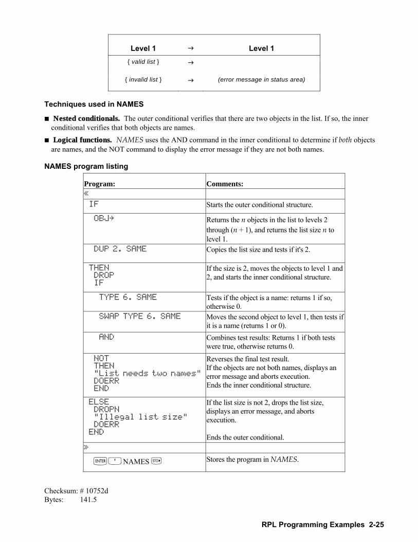
RPL Programming Examples 2-25
Level 1 " Level 1 valid list "
invalid list " (error message in status area)
Techniques used in NAMES
! Nested conditionals. The outer conditional verifies that there are two objects in the list. If so, the inner conditional verifies that both objects are names.
! Logical functions. NAMES uses the AND command in the inner conditional to determine if both objects are names, and the NOT command to display the error message if they are not both names.
NAMES program listing
Program: Comments: « IF Starts the outer conditional structure.
OBJ Returns the n objects in the list to levels 2 through (n + 1), and returns the list size n to level 1.
DUP 2. SAME Copies the list size and tests if it's 2.
THEN DROP IF
If the size is 2, moves the objects to level 1 and 2, and starts the inner conditional structure.
TYPE 6. SAME Tests if the object is a name: returns 1 if so, otherwise 0.
SWAP TYPE 6. SAME Moves the second object to level 1, then tests if it is a name (returns 1 or 0).
AND Combines test results: Returns 1 if both tests were true, otherwise returns 0.
NOT THEN "List needs two names" DOERR END
Reverses the final test result. If the objects are not both names, displays an error message and aborts execution. Ends the inner conditional structure.
ELSE DROPN "Illegal list size" DOERR END
If the list size is not 2, drops the list size, displays an error message, and aborts execution. Ends the outer conditional.
»
`ONAMES K Stores the program in NAMES.
Checksum: # 10752d Bytes: 141.5
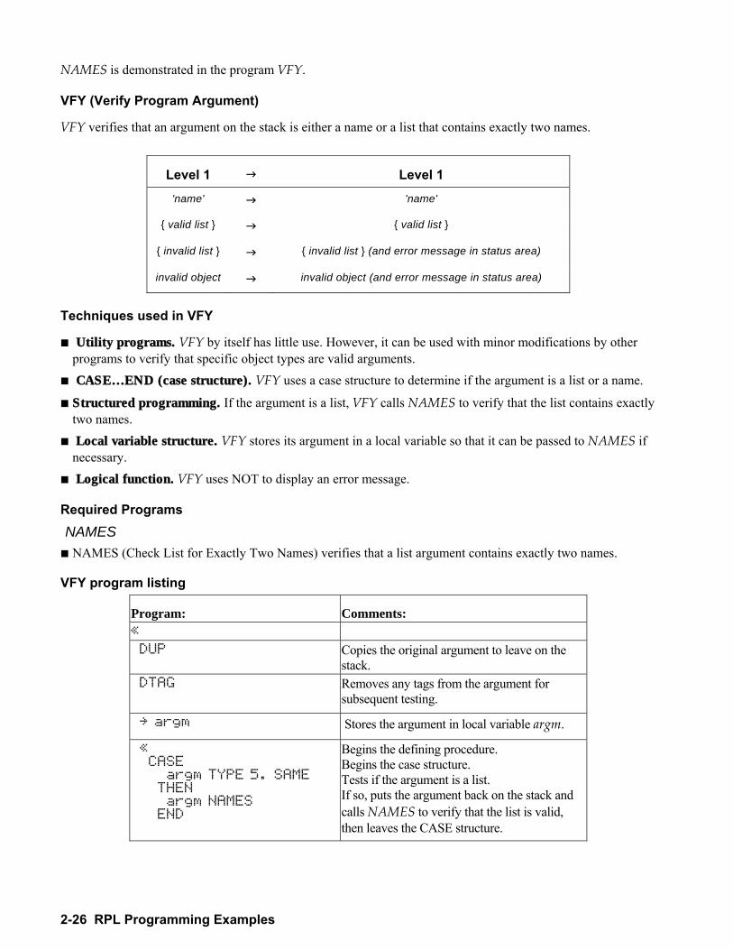
2-26 RPL Programming Examples
NAMES is demonstrated in the program VFY.
VFY (Verify Program Argument)
VFY verifies that an argument on the stack is either a name or a list that contains exactly two names.
Level 1 " Level 1
'name' " 'name'
valid list " valid list
invalid list " invalid list (and error message in status area)
invalid object " invalid object (and error message in status area)
Techniques used in VFY
! Utility programs. VFY by itself has little use. However, it can be used with minor modifications by other programs to verify that specific object types are valid arguments.
! CASE…END (case structure). VFY uses a case structure to determine if the argument is a list or a name.
! Structured programming. If the argument is a list, VFY calls NAMES to verify that the list contains exactly two names.
! Local variable structure. VFY stores its argument in a local variable so that it can be passed to NAMES if necessary.
! Logical function. VFY uses NOT to display an error message.
Required Programs NAMES ! NAMES (Check List for Exactly Two Names) verifies that a list argument contains exactly two names.
VFY program listing
Program: Comments: « DUP Copies the original argument to leave on the
stack. DTAG Removes any tags from the argument for
subsequent testing.
argm Stores the argument in local variable argm.
« CASE argm TYPE 5. SAME THEN argm NAMES END
Begins the defining procedure. Begins the case structure. Tests if the argument is a list. If so, puts the argument back on the stack and calls NAMES to verify that the list is valid, then leaves the CASE structure.
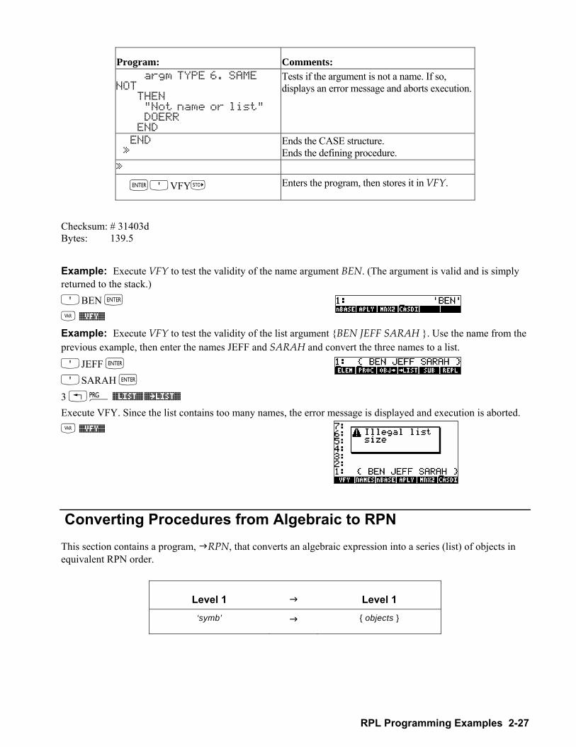
RPL Programming Examples 2-27
Program: Comments: argm TYPE 6. SAME NOT THEN "Not name or list" DOERR END
Tests if the argument is not a name. If so, displays an error message and aborts execution.
END »
Ends the CASE structure. Ends the defining procedure.
»
`OVFYK Enters the program, then stores it in VFY.
Checksum: # 31403d Bytes: 139.5
Example: Execute VFY to test the validity of the name argument BEN. (The argument is valid and is simply returned to the stack.) OBEN ` J %VFY% Example: Execute VFY to test the validity of the list argument BEN JEFF SARAH . Use the name from the previous example, then enter the names JEFF and SARAH and convert the three names to a list. OJEFF ` OSARAH `
3 !° %LIST% %²LIST%
Execute VFY. Since the list contains too many names, the error message is displayed and execution is aborted. J %VFY%
Converting Procedures from Algebraic to RPN This section contains a program, "RPN, that converts an algebraic expression into a series (list) of objects in equivalent RPN order.
Level 1 " Level 1 ‘symb’ " objects
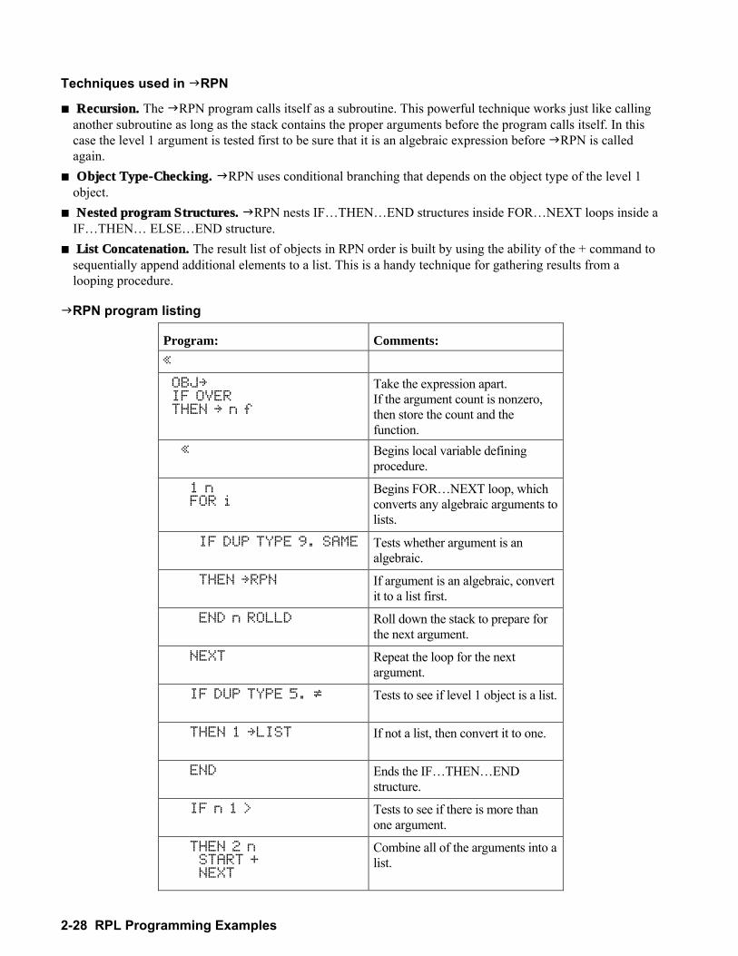
2-28 RPL Programming Examples
Techniques used in "RPN
! Recursion. The "RPN program calls itself as a subroutine. This powerful technique works just like calling another subroutine as long as the stack contains the proper arguments before the program calls itself. In this case the level 1 argument is tested first to be sure that it is an algebraic expression before "RPN is called again.
! Object Type-Checking. "RPN uses conditional branching that depends on the object type of the level 1 object.
! Nested program Structures. "RPN nests IFTHENEND structures inside FORNEXT loops inside a IFTHEN ELSEEND structure.
! List Concatenation. The result list of objects in RPN order is built by using the ability of the + command to sequentially append additional elements to a list. This is a handy technique for gathering results from a looping procedure.
"RPN program listing
Program: Comments: « OBJ IF OVER THEN n f
Take the expression apart. If the argument count is nonzero, then store the count and the function.
« Begins local variable defining procedure.
1 n FOR i
Begins FORNEXT loop, which converts any algebraic arguments to lists.
IF DUP TYPE 9. SAME Tests whether argument is an algebraic.
THEN RPN If argument is an algebraic, convert it to a list first.
END n ROLLD Roll down the stack to prepare for the next argument.
NEXT Repeat the loop for the next argument.
IF DUP TYPE 5. ‹ Tests to see if level 1 object is a list.
THEN 1 LIST If not a list, then convert it to one.
END Ends the IFTHENEND structure.
IF n 1 > Tests to see if there is more than one argument.
THEN 2 n START + NEXT
Combine all of the arguments into a list.
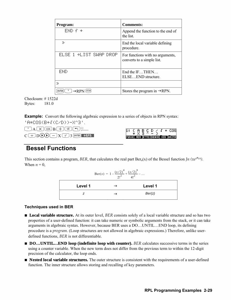
RPL Programming Examples 2-29
Program: Comments: END f + Append the function to the end of
the list.
» End the local variable defining procedure.
ELSE 1 LIST SWAP DROP For functions with no arguments, converts to a simple list.
END End the IFTHEN ELSEEND structure.
»
`O"RPN K Stores the program in "RPN.
Checksum: # 1522d Bytes: 181.0 Example: Convert the following algebraic expression to a series of objects in RPN syntax: 'A*COS(B+ƒ(C/D))-X^3'. OA *TB +R!Ü
C /D -X Q3 `%²RPN%
Bessel Functions This section contains a program, BER, that calculates the real part Bern(x) of the Bessel function Jn (xe3πi/4). When n = 0,
Ber x( ) 1 x 2⁄( )4
2!2----------------- x 2⁄( )8
4!2----------------- …+=
Level 1 " Level 1 z " Ber(z)
Techniques used in BER
! Local variable structure. At its outer level, BER consists solely of a local variable structure and so has two properties of a user-defined function: it can take numeric or symbolic arguments from the stack, or it can take arguments in algebraic syntax. However, because BER uses a DOUNTILEND loop, its defining procedure is a program. (Loop structures are not allowed in algebraic expressions.) Therefore, unlike user-defined functions, BER is not differentiable.
! DO…UNTIL…END loop (indefinite loop with counter). BER calculates successive terms in the series using a counter variable. When the new term does not differ from the previous term to within the 12-digit precision of the calculator, the loop ends.
! Nested local variable structures. The outer structure is consistent with the requirements of a user-defined function. The inner structure allows storing and recalling of key parameters.
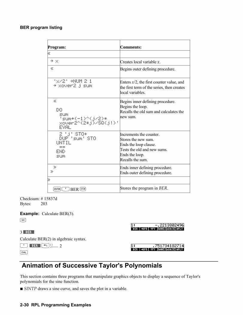
2-30 RPL Programming Examples
BER program listing
Program: Comments: « x Creates local variable x. « Begins outer defining procedure.
'x/2' NUM 2 1 xover2 j sum
Enters x/2, the first counter value, and the first term of the series, then creates local variables.
« DO sum 'sum+(-1)^(j/2)* xover2^(2*j)/SQ(j!)' EVAL
Begins inner defining procedure. Begins the loop. Recalls the old sum and calculates the new sum.
2 'j' STO+ DUP 'sum' STO UNTIL == END sum
Increments the counter. Stores the new sum. Ends the loop clause. Tests the old and new sums. Ends the loop. Recalls the sum.
» »
Ends inner defining procedure. Ends outer defining procedure.
»
`OBER K Stores the program in BER.
Checksum: # 15837d Bytes: 203
Example: Calculate BER(3). J 3 %BER%
Calculate BER(2) in algebraic syntax. O %BER% !Ü2 N
Animation of Successive Taylor's Polynomials This section contains three programs that manipulate graphics objects to display a sequence of Taylor's polynomials for the sine function. ! SINTP draws a sine curve, and saves the plot in a variable.
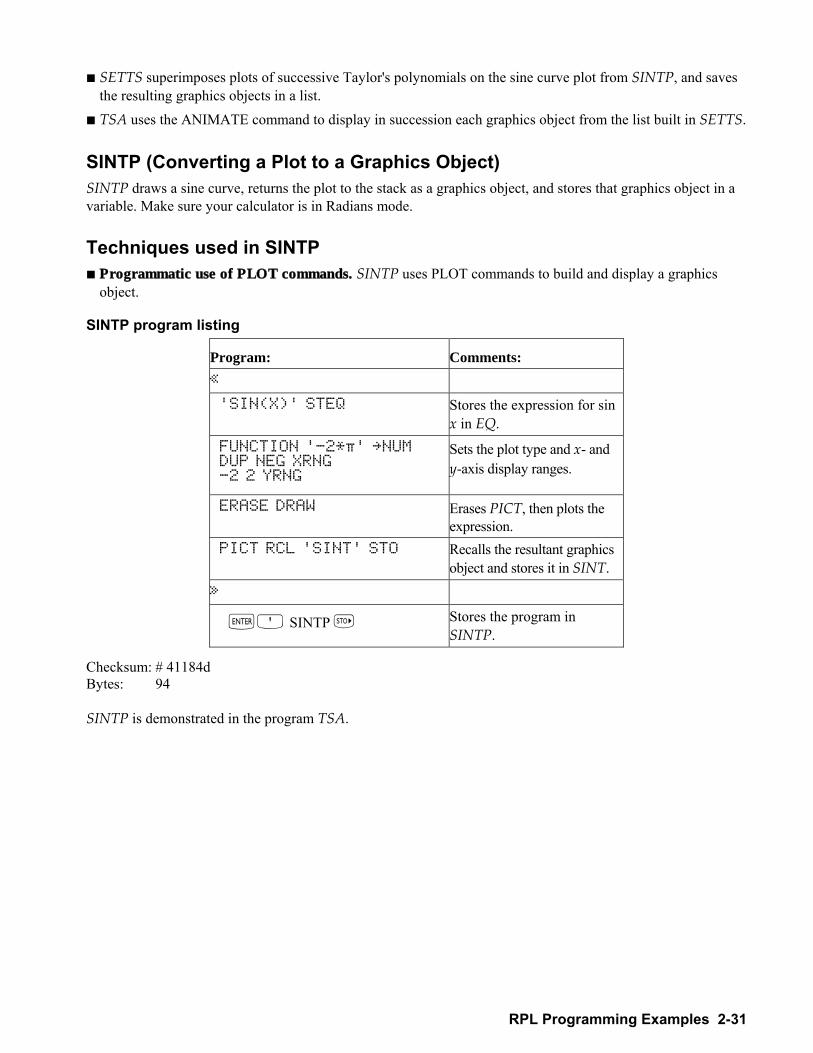
RPL Programming Examples 2-31
! SETTS superimposes plots of successive Taylor's polynomials on the sine curve plot from SINTP, and saves the resulting graphics objects in a list.
! TSA uses the ANIMATE command to display in succession each graphics object from the list built in SETTS. SINTP (Converting a Plot to a Graphics Object) SINTP draws a sine curve, returns the plot to the stack as a graphics object, and stores that graphics object in a variable. Make sure your calculator is in Radians mode. Techniques used in SINTP ! Programmatic use of PLOT commands. SINTP uses PLOT commands to build and display a graphics
object.
SINTP program listing
Program: Comments: « 'SIN(X)' STEQ Stores the expression for sin
x in EQ. FUNCTION '-2*‡' NUM DUP NEG XRNG -2 2 YRNG
Sets the plot type and x- and y-axis display ranges.
ERASE DRAW Erases PICT, then plots the expression.
PICT RCL 'SINT' STO Recalls the resultant graphics object and stores it in SINT.
»
`O SINTP K Stores the program in SINTP.
Checksum: # 41184d Bytes: 94
SINTP is demonstrated in the program TSA.
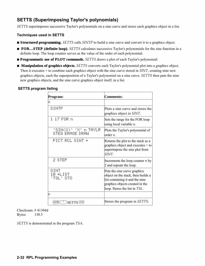
2-32 RPL Programming Examples
SETTS (Superimposing Taylor's polynomials) SETTS superimposes successive Taylor's polynomials on a sine curve and stores each graphics object in a list.
Techniques used in SETTS
! Structured programming. SETTS calls SINTP to build a sine curve and convert it to a graphics object.
! FOR…STEP (definite loop). SETTS calculates successive Taylor's polynomials for the sine function in a definite loop. The loop counter serves as the value of the order of each polynomial.
! Programmatic use of PLOT commands. SETTS draws a plot of each Taylor's polynomial.
! Manipulation of graphics objects. SETTS converts each Taylor's polynomial plot into a graphics object. Then it executes + to combine each graphics object with the sine curve stored in SINT, creating nine new graphics objects, each the superposition of a Taylor's polynomial on a sine curve. SETTS then puts the nine new graphics objects, and the sine curve graphics object itself, in a list.
SETTS program listing
Program: Comments: « SINTP Plots a sine curve and stores the
graphics object in SINT. 1 17 FOR n Sets the range for the FOR loop
using local variable n. 'SIN(X)' 'X' n TAYLR STEQ ERASE DRAW
Plots the Taylor's polynomial of order n.
PICT RCL SINT + Returns the plot to the stack as a graphics object and executes + to superimpose the sine plot from SINT.
2 STEP Increments the loop counter n by 2 and repeats the loop.
SINT 10 LIST 'TSL' STO
Puts the sine curve graphics object on the stack, then builds a list containing it and the nine graphics objects created in the loop. Stores the list in TSL.
»
`OSETTS K Stores the program in SETTS.
Checksum: # 41304d Bytes: 130.5
SETTS is demonstrated in the program TSA.
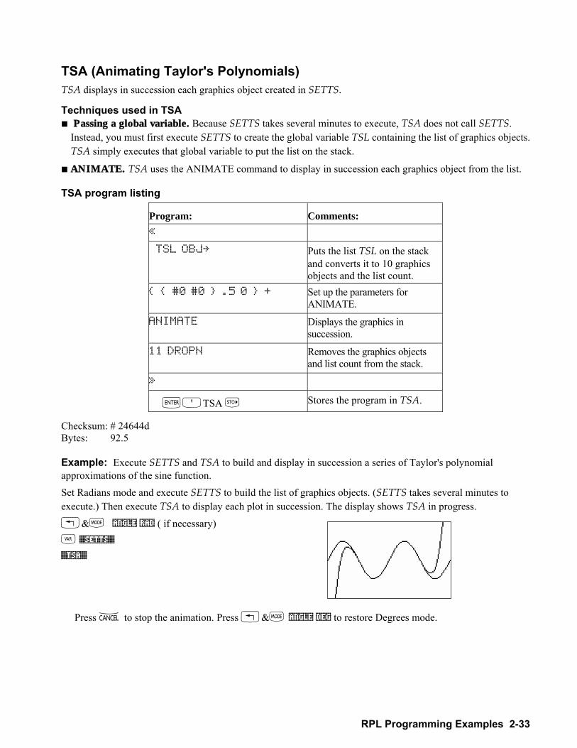
RPL Programming Examples 2-33
TSA (Animating Taylor's Polynomials) TSA displays in succession each graphics object created in SETTS.
Techniques used in TSA ! Passing a global variable. Because SETTS takes several minutes to execute, TSA does not call SETTS.
Instead, you must first execute SETTS to create the global variable TSL containing the list of graphics objects. TSA simply executes that global variable to put the list on the stack.
! ANIMATE. TSA uses the ANIMATE command to display in succession each graphics object from the list.
TSA program listing
Program: Comments: « TSL OBJ Puts the list TSL on the stack
and converts it to 10 graphics objects and the list count.
#0 #0 .5 0 + Set up the parameters for ANIMATE.
ANIMATE Displays the graphics in succession.
11 DROPN Removes the graphics objects and list count from the stack.
»
`OTSA K Stores the program in TSA.
Checksum: # 24644d Bytes: 92.5
Example: Execute SETTS and TSA to build and display in succession a series of Taylor's polynomial approximations of the sine function. Set Radians mode and execute SETTS to build the list of graphics objects. (SETTS takes several minutes to execute.) Then execute TSA to display each plot in succession. The display shows TSA in progress.
!&H !ANGLE !RAD ( if necessary) J %SETTS%
%TSA%
Press − to stop the animation. Press !&H !ANGLE !DEG to restore Degrees mode.
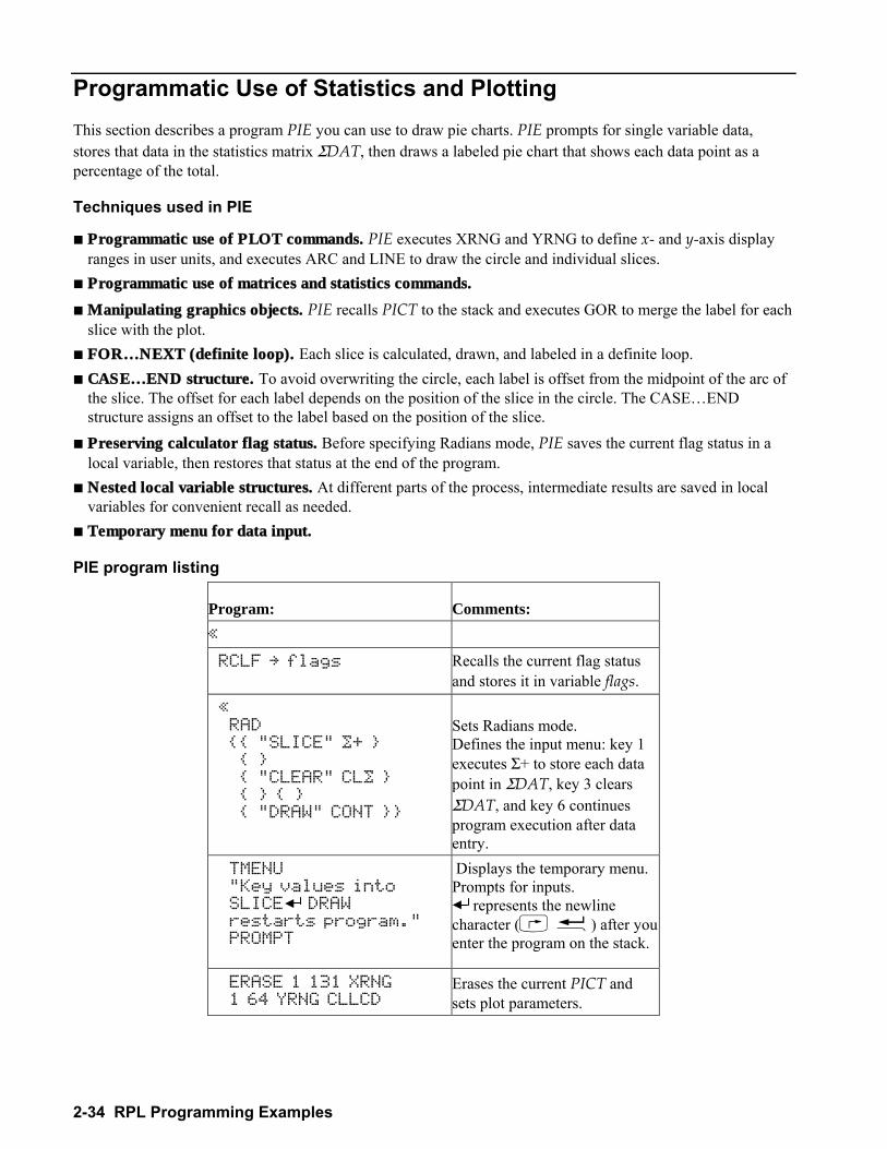
2-34 RPL Programming Examples
Programmatic Use of Statistics and Plotting This section describes a program PIE you can use to draw pie charts. PIE prompts for single variable data, stores that data in the statistics matrix ΣDAT, then draws a labeled pie chart that shows each data point as a percentage of the total.
Techniques used in PIE
! Programmatic use of PLOT commands. PIE executes XRNG and YRNG to define x- and y-axis display ranges in user units, and executes ARC and LINE to draw the circle and individual slices.
! Programmatic use of matrices and statistics commands.
! Manipulating graphics objects. PIE recalls PICT to the stack and executes GOR to merge the label for each slice with the plot.
! FOR…NEXT (definite loop). Each slice is calculated, drawn, and labeled in a definite loop. ! CASE…END structure. To avoid overwriting the circle, each label is offset from the midpoint of the arc of
the slice. The offset for each label depends on the position of the slice in the circle. The CASEEND structure assigns an offset to the label based on the position of the slice.
! Preserving calculator flag status. Before specifying Radians mode, PIE saves the current flag status in a local variable, then restores that status at the end of the program.
! Nested local variable structures. At different parts of the process, intermediate results are saved in local variables for convenient recall as needed.
! Temporary menu for data input.
PIE program listing
Program: Comments: «
RCLF flags Recalls the current flag status and stores it in variable flags.
« RAD "SLICE" …+ "CLEAR" CL… "DRAW" CONT
Sets Radians mode. Defines the input menu: key 1 executes Σ+ to store each data point in ΣDAT, key 3 clears ΣDAT, and key 6 continues program execution after data entry.
TMENU "Key values into SLICE DRAW restarts program." PROMPT
Displays the temporary menu. Prompts for inputs.
represents the newline character ( ë) after you enter the program on the stack.
ERASE 1 131 XRNG 1 64 YRNG CLLCD
Erases the current PICT and sets plot parameters.
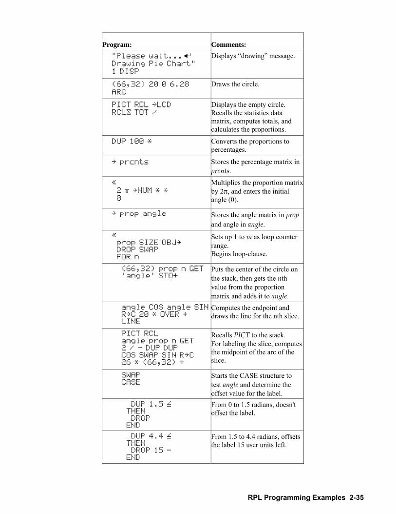
RPL Programming Examples 2-35
Program: Comments: "Please wait... Drawing Pie Chart" 1 DISP
Displays drawing message.
(66,32) 20 0 6.28 ARC
Draws the circle.
PICT RCL LCD RCL… TOT /
Displays the empty circle. Recalls the statistics data matrix, computes totals, and calculates the proportions.
DUP 100 * Converts the proportions to percentages.
prcnts Stores the percentage matrix in prcnts.
« 2 ‡ NUM * * 0
Multiplies the proportion matrix by 2π, and enters the initial angle (0).
prop angle Stores the angle matrix in prop and angle in angle.
« prop SIZE OBJ DROP SWAP FOR n
Sets up 1 to m as loop counter range. Begins loop-clause.
(66,32) prop n GET 'angle' STO+
Puts the center of the circle on the stack, then gets the nth value from the proportion matrix and adds it to angle.
angle COS angle SIN RC 20 * OVER + LINE
Computes the endpoint and draws the line for the nth slice.
PICT RCL angle prop n GET 2 / - DUP DUP COS SWAP SIN RC 26 * (66,32) +
Recalls PICT to the stack. For labeling the slice, computes the midpoint of the arc of the slice.
SWAP CASE
Starts the CASE structure to test angle and determine the offset value for the label.
DUP 1.5 ‰ THEN DROP END
From 0 to 1.5 radians, doesn't offset the label.
DUP 4.4 ‰ THEN DROP 15 - END
From 1.5 to 4.4 radians, offsets the label 15 user units left.
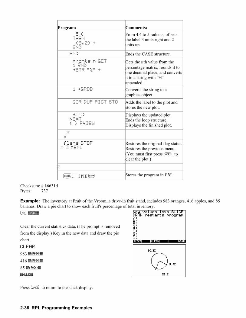
2-36 RPL Programming Examples
Program: Comments: 5 < THEN (3,2) + END
From 4.4 to 5 radians, offsets the label 3 units right and 2 units up.
END Ends the CASE structure. prcnts n GET 1 RND STR "%" +
Gets the nth value from the percentage matrix, rounds it to one decimal place, and converts it to a string with % appended.
1 GROB Converts the string to a graphics object.
GOR DUP PICT STO Adds the label to the plot and stores the new plot.
LCD NEXT PVIEW
Displays the updated plot. Ends the loop structure. Displays the finished plot.
» »
flags STOF » 0 MENU
Restores the original flag status. Restores the previous menu. (You must first press − to clear the plot.)
»
`OPIE K Stores the program in PIE.
Checksum: # 16631d Bytes: 737
Example: The inventory at Fruit of the Vroom, a drive-in fruit stand, includes 983 oranges, 416 apples, and 85 bananas. Draw a pie chart to show each fruit's percentage of total inventory. J %PIE% Clear the current statistics data. (The prompt is removed from the display.) Key in the new data and draw the pie chart. CLEAR 983 %SLICE%
416 %SLICE%
85 %SLICE%
%DRAW%
Press − to return to the stack display.
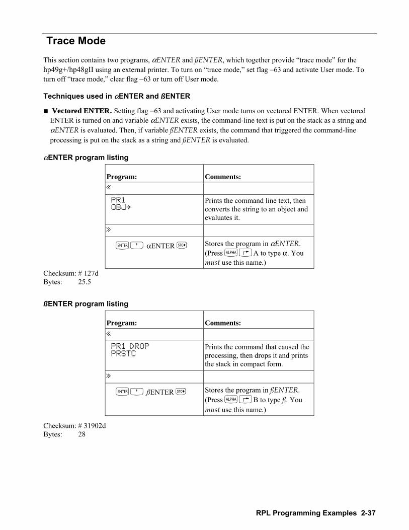
RPL Programming Examples 2-37
Trace Mode This section contains two programs, αENTER and ßENTER, which together provide trace mode for the hp49g+/hp48gII using an external printer. To turn on trace mode, set flag 63 and activate User mode. To turn off trace mode, clear flag 63 or turn off User mode.
Techniques used in αENTER and ßENTER
! Vectored ENTER. Setting flag 63 and activating User mode turns on vectored ENTER. When vectored ENTER is turned on and variable αENTER exists, the command-line text is put on the stack as a string and αENTER is evaluated. Then, if variable ßENTER exists, the command that triggered the command-line processing is put on the stack as a string and ßENTER is evaluated.
αENTER program listing
Checksum: # 127d Bytes: 25.5
ßENTER program listing
Program: Comments: « PR1 DROP PRSTC
Prints the command that caused the processing, then drops it and prints the stack in compact form.
»
`O ßENTER K Stores the program in ßENTER. (Press ~B to type ß. You must use this name.)
Checksum: # 31902d Bytes: 28
Program: Comments: « PR1 OBJ
Prints the command line text, then converts the string to an object and evaluates it.
»
`O αENTER K Stores the program in αENTER. (Press ~A to type α. You must use this name.)
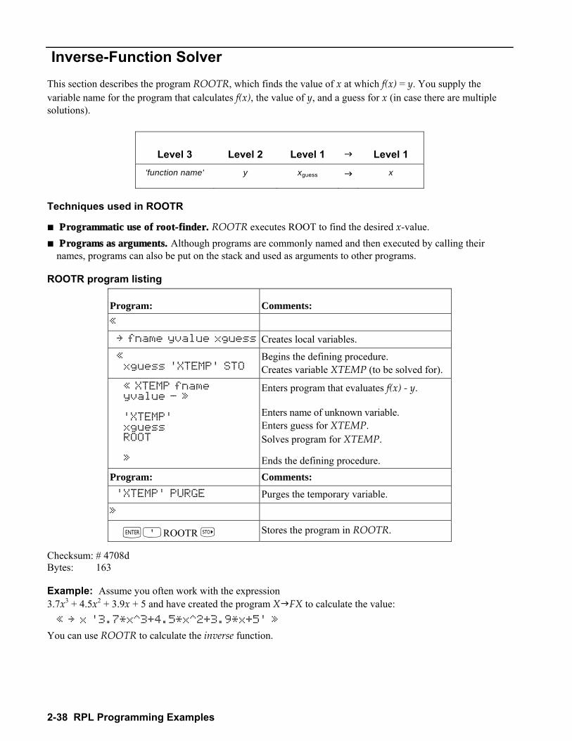
2-38 RPL Programming Examples
Inverse-Function Solver This section describes the program ROOTR, which finds the value of x at which f(x) = y. You supply the variable name for the program that calculates f(x), the value of y, and a guess for x (in case there are multiple solutions).
Level 3 Level 2 Level 1 " Level 1 'function name' y xguess " x
Techniques used in ROOTR
! Programmatic use of root-finder. ROOTR executes ROOT to find the desired x-value. ! Programs as arguments. Although programs are commonly named and then executed by calling their
names, programs can also be put on the stack and used as arguments to other programs.
ROOTR program listing
Program: Comments: « fname yvalue xguess Creates local variables. « xguess 'XTEMP' STO
Begins the defining procedure. Creates variable XTEMP (to be solved for).
« XTEMP fname yvalue - » 'XTEMP' xguess ROOT »
Enters program that evaluates f(x) - y. Enters name of unknown variable. Enters guess for XTEMP. Solves program for XTEMP. Ends the defining procedure.
Program: Comments: 'XTEMP' PURGE Purges the temporary variable. »
`OROOTR K Stores the program in ROOTR.
Checksum: # 4708d Bytes: 163
Example: Assume you often work with the expression 3.7x3 + 4.5x2 + 3.9x + 5 and have created the program X"FX to calculate the value: « x '3.7*x^3+4.5*x^2+3.9*x+5' »
You can use ROOTR to calculate the inverse function.
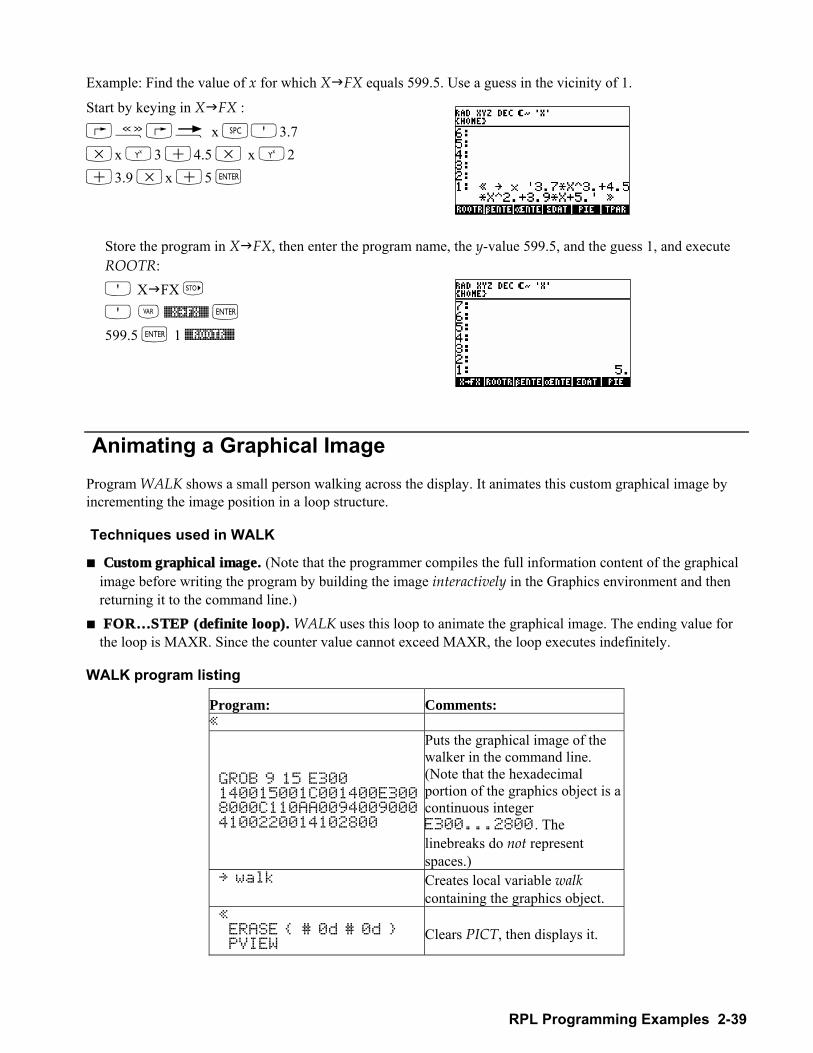
RPL Programming Examples 2-39
Example: Find the value of x for which X"FX equals 599.5. Use a guess in the vicinity of 1.
Start by keying in X"FX :
@å@é x O3.7 *x Q3 +4.5 * x Q2 +3.9 *x +5 `
Store the program in X"FX, then enter the program name, the y-value 599.5, and the guess 1, and execute ROOTR: O X"FX K O J %X²FX% `
599.5 ` 1 %ROOTR%
Animating a Graphical Image Program WALK shows a small person walking across the display. It animates this custom graphical image by incrementing the image position in a loop structure.
Techniques used in WALK
! Custom graphical image. (Note that the programmer compiles the full information content of the graphical image before writing the program by building the image interactively in the Graphics environment and then returning it to the command line.)
! FOR…STEP (definite loop). WALK uses this loop to animate the graphical image. The ending value for the loop is MAXR. Since the counter value cannot exceed MAXR, the loop executes indefinitely.
WALK program listing
Program: Comments: «
GROB 9 15 E300 140015001C001400E300 8000C110AA0094009000 4100220014102800
Puts the graphical image of the walker in the command line. (Note that the hexadecimal portion of the graphics object is a continuous integer E300...2800. The linebreaks do not represent spaces.)
walk Creates local variable walk containing the graphics object.
« ERASE # 0d # 0d PVIEW
Clears PICT, then displays it.
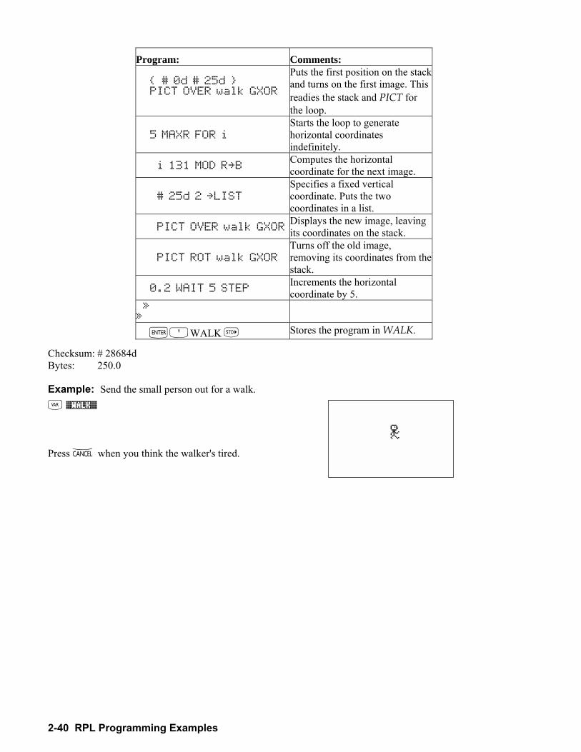
2-40 RPL Programming Examples
Program: Comments:
# 0d # 25d PICT OVER walk GXOR
Puts the first position on the stack and turns on the first image. This readies the stack and PICT for the loop.
5 MAXR FOR i Starts the loop to generate horizontal coordinates indefinitely.
i 131 MOD RB Computes the horizontal coordinate for the next image.
# 25d 2 LIST Specifies a fixed vertical coordinate. Puts the two coordinates in a list.
PICT OVER walk GXORDisplays the new image, leaving its coordinates on the stack.
PICT ROT walk GXOR Turns off the old image, removing its coordinates from the stack.
0.2 WAIT 5 STEP Increments the horizontal coordinate by 5.
» »
`OWALK K Stores the program in WALK.
Checksum: # 28684d Bytes: 250.0
Example: Send the small person out for a walk. J %WALK%
Press − when you think the walker's tired.
3
RPL Programming Examples 3-1
3.Full Command and Function Reference Introduction This chapter details the hp49g+/hp48gII commands and functions. These listings include the following information: ! a brief definition of what the command or function does ! additional information about how it works and how to use it ! the key to press to gain access to it ! any flags that may affect how it works ! a stack diagram showing the arguments it requires (if any) ! related commands or functions
Computer Algebra System Commands and Functions
CAS-specific commands and functions are included in this chapter with a description of what the item does. For more detailed information on CAS-specific items, see the listing for each CAS item in the next chapter. For example, the CAS command ABCUV is included in this chapter, but the only description given is:
CAS: From polynomials a, b and constant c give polynomials u and v such that au+bv =c . The CAS: indicates that this is a computer algebra system item and that the next chapter contains a listing giving more information on the entry.
How to Access Commands and Functions
Many of the commands and functions in this reference are not located on the hp49g+/hp48gII keyboard and are accessed by pressing µ. This is the right-shifted function of the Pkey, which is the fourth key from the left on the fourth row of keys from the top. Once accessed, the function or commands name is found by pressing the ~key and then using the letter keys to spell out the function or commands name. Usually, pressing the first letter of the command will move the catalog list close enough to the function to use the key to find the function. For functions or commands (or symbols) that are located on the hp49g+/hp48gII keyboard as shifted functions of other keys (such as µ above), the proper shift key is shown followed by a font symbol indicating the function, command or symbol written above the key.
In some cases, access is shown with two keys with an ampersand (&) in between, such as !&H. This notation means that you must press the first key and hold it down while then pressing the second key at the same time. The next few pages explain how to read the stack diagrams in the command reference, how commands are alphabetized, and the meaning of command classifications at the upper right corner of each stack diagram.
How to Read Stack Diagrams
Each entry in the command reference includes a stack diagram. This is a table showing the arguments that the command, function, or analytic function takes from the stack and the results that it returns to the stack. The " character (pronounced to as in to list for "List) in the table separates the arguments from the results. The stack diagram for a command may contain more than one argument " result line, reflecting all possible combinations of arguments and results for that command.
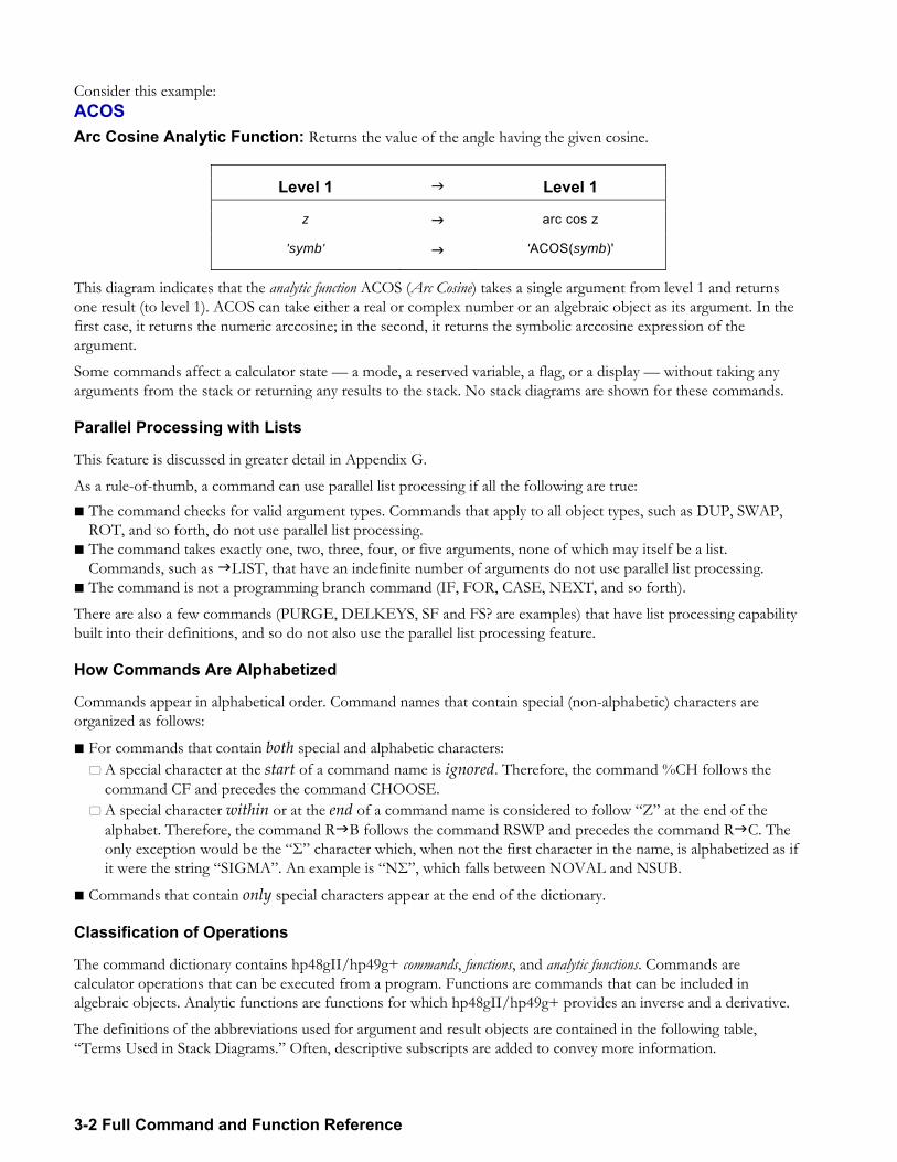
3-2 Full Command and Function Reference
Consider this example: ACOS Arc Cosine Analytic Function: Returns the value of the angle having the given cosine.
Level 1 " Level 1
z " arc cos z
'symb' " 'ACOS(symb)'
This diagram indicates that the analytic function ACOS (Arc Cosine) takes a single argument from level 1 and returns one result (to level 1). ACOS can take either a real or complex number or an algebraic object as its argument. In the first case, it returns the numeric arccosine; in the second, it returns the symbolic arccosine expression of the argument.
Some commands affect a calculator state a mode, a reserved variable, a flag, or a display without taking any arguments from the stack or returning any results to the stack. No stack diagrams are shown for these commands.
Parallel Processing with Lists
This feature is discussed in greater detail in Appendix G.
As a rule-of-thumb, a command can use parallel list processing if all the following are true: ! The command checks for valid argument types. Commands that apply to all object types, such as DUP, SWAP,
ROT, and so forth, do not use parallel list processing. ! The command takes exactly one, two, three, four, or five arguments, none of which may itself be a list.
Commands, such as "LIST, that have an indefinite number of arguments do not use parallel list processing. ! The command is not a programming branch command (IF, FOR, CASE, NEXT, and so forth).
There are also a few commands (PURGE, DELKEYS, SF and FS? are examples) that have list processing capability built into their definitions, and so do not also use the parallel list processing feature.
How Commands Are Alphabetized
Commands appear in alphabetical order. Command names that contain special (non-alphabetic) characters are organized as follows:
! For commands that contain both special and alphabetic characters: " A special character at the start of a command name is ignored. Therefore, the command %CH follows the
command CF and precedes the command CHOOSE. " A special character within or at the end of a command name is considered to follow Z at the end of the
alphabet. Therefore, the command R"B follows the command RSWP and precedes the command R"C. The only exception would be the Σ character which, when not the first character in the name, is alphabetized as if it were the string SIGMA. An example is NΣ, which falls between NOVAL and NSUB.
! Commands that contain only special characters appear at the end of the dictionary.
Classification of Operations
The command dictionary contains hp48gII/hp49g+ commands, functions, and analytic functions. Commands are calculator operations that can be executed from a program. Functions are commands that can be included in algebraic objects. Analytic functions are functions for which hp48gII/hp49g+ provides an inverse and a derivative.
The definitions of the abbreviations used for argument and result objects are contained in the following table, Terms Used in Stack Diagrams. Often, descriptive subscripts are added to convey more information.
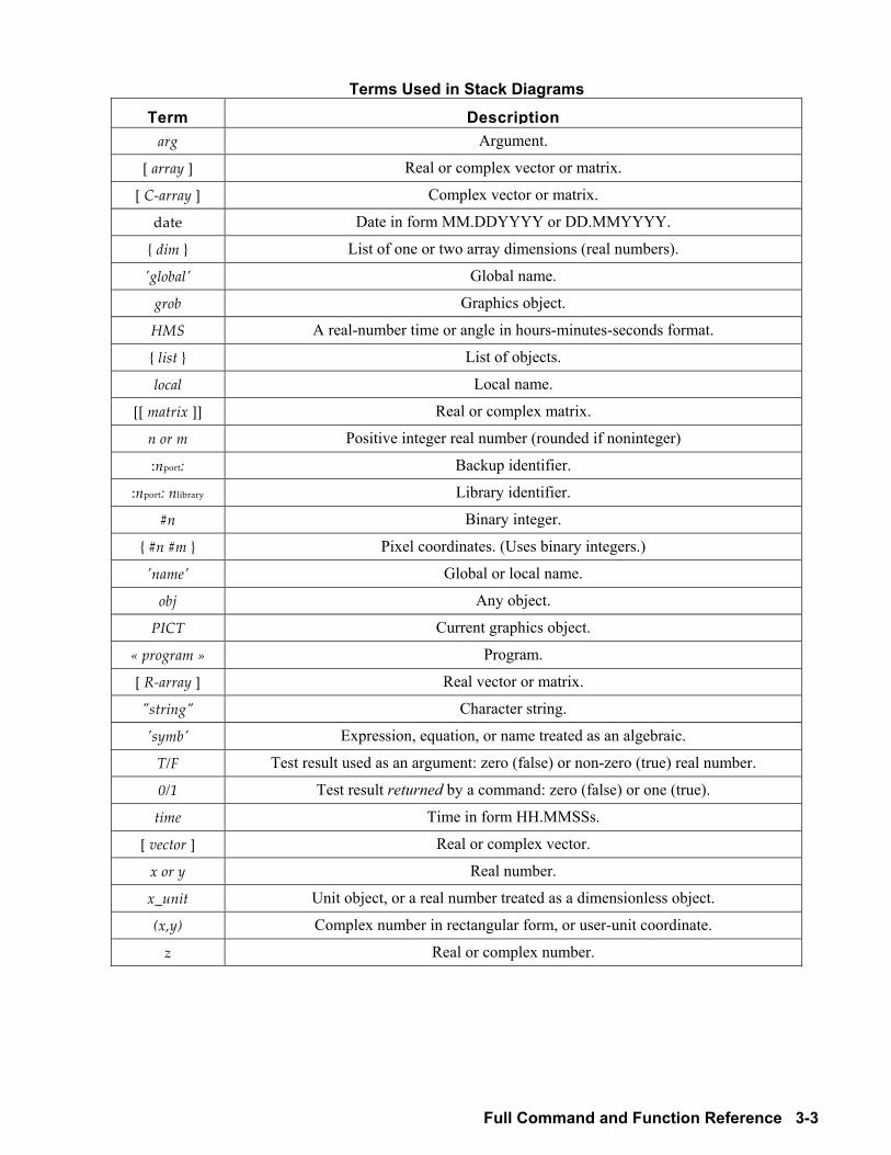
Full Command and Function Reference 3-3
Terms Used in Stack Diagrams
Term Descriptionarg Argument.
[ array ] Real or complex vector or matrix.
[ C-array ] Complex vector or matrix.
date Date in form MM.DDYYYY or DD.MMYYYY.
dim List of one or two array dimensions (real numbers).
'global' Global name.
grob Graphics object.
HMS A real-number time or angle in hours-minutes-seconds format.
list List of objects.
local Local name.
[[ matrix ]] Real or complex matrix.
n or m Positive integer real number (rounded if noninteger)
:nport: Backup identifier.
:nport: nlibrary Library identifier.
#n Binary integer.
#n #m Pixel coordinates. (Uses binary integers.)
'name' Global or local name.
obj Any object.
PICT Current graphics object.
« program » Program.
[ R-array ] Real vector or matrix.
"string" Character string.
'symb' Expression, equation, or name treated as an algebraic.
T/F Test result used as an argument: zero (false) or non-zero (true) real number.
0/1 Test result returned by a command: zero (false) or one (true).
time Time in form HH.MMSSs.
[ vector ] Real or complex vector.
x or y Real number.
x_unit Unit object, or a real number treated as a dimensionless object.
(x,y) Complex number in rectangular form, or user-unit coordinate.
z Real or complex number.
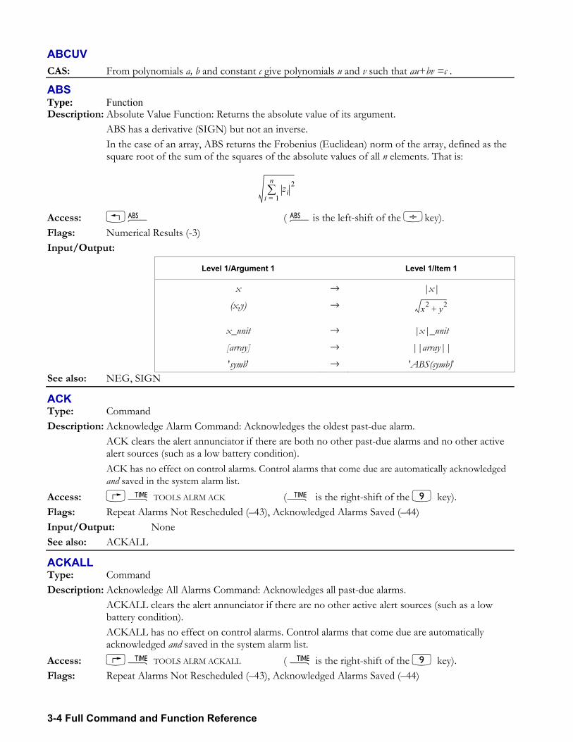
3-4 Full Command and Function Reference
ABCUV CAS: From polynomials a, b and constant c give polynomials u and v such that au+bv =c .
ABS Type: Function Description: Absolute Value Function: Returns the absolute value of its argument. ABS has a derivative (SIGN) but not an inverse. In the case of an array, ABS returns the Frobenius (Euclidean) norm of the array, defined as the
square root of the sum of the squares of the absolute values of all n elements. That is:
zi2
i 1=
n∑
Access: !Ê ( Êis the left-shift of the /key). Flags: Numerical Results (-3) Input/Output:
Level 1/Argument 1 Level 1/Item 1
x → |x| (x,y) → x2 y2+
x_unit → |x|_unit [array] → ||array|| 'symb' → 'ABS(symb)'
See also: NEG, SIGN
ACK Type: Command Description: Acknowledge Alarm Command: Acknowledges the oldest past-due alarm. ACK clears the alert annunciator if there are both no other past-due alarms and no other active
alert sources (such as a low battery condition). ACK has no effect on control alarms. Control alarms that come due are automatically acknowledged
and saved in the system alarm list. Access: Ó TOOLS ALRM ACK (Ó is the right-shift of the 9 key). Flags: Repeat Alarms Not Rescheduled (43), Acknowledged Alarms Saved (44) Input/Output: None See also: ACKALL
ACKALL Type: Command Description: Acknowledge All Alarms Command: Acknowledges all past-due alarms. ACKALL clears the alert annunciator if there are no other active alert sources (such as a low
battery condition). ACKALL has no effect on control alarms. Control alarms that come due are automatically
acknowledged and saved in the system alarm list. Access: Ó TOOLS ALRM ACKALL ( Ó is the right-shift of the 9 key). Flags: Repeat Alarms Not Rescheduled (43), Acknowledged Alarms Saved (44)
Full Command and Function Reference 3-5
Input/Output: None See also: ACK
ACOS Type: Analytic Function Description: Arc Cosine Analytic Function: Returns the value of the angle having the given cosine. For a real argument x in the domain 1 ≤ x ≤ 1, the result ranges from 0 to 180 degrees (0 to π
radians; 0 to 200 grads). A real argument outside of this domain is converted to a complex argument, z = x + 0i, and the
result is complex. The inverse of COS is a relation, not a function, since COS sends more than one argument to the
same result. The inverse relation for COS is expressed by ISOL as the general solution s1*ACOS(Z)+2*π*n1
The function ACOS is the inverse of a part of COS, a part defined by restricting the domain of COS such that: each argument is sent to a distinct result, and each possible result is achieved.
The points in this restricted domain of COS are called the principal values of the inverse relation. ACOS in its entirety is called the principal branch of the inverse relation, and the points sent by ACOS to the boundary of the restricted domain of COS form the branch cuts of ACOS.
The principal branch used by the hp49g+/hp48gII for ACOS was chosen because it is analytic in the regions where the arguments of the real-valued inverse function are defined. The branch cut for the complex-valued arc cosine function occurs where the corresponding real-valued function is undefined. The principal branch also preserves most of the important symmetries.
The graphs below show the domain and range of ACOS. The graph of the domain shows where the branch cuts occur: the heavy solid line marks one side of a cut, while the feathered lines mark the other side of a cut. The graph of the range shows where each side of each cut is mapped under the function.
These graphs show the inverse relation s1*ACOS(Z)+2*π*n1 for the case s1=1 and n1 = 0. For other values of s1 and n1, the vertical band in the lower graph is translated to the right or to the left. Taken together, the bands cover the whole complex plane, which is the domain of COS.
View these graphs with domain and range reversed to see how the domain of COS is restricted to make an inverse function possible. Consider the vertical band in the lower graph as the restricted domain Z = (x, y). COS sends this domain onto the whole complex plane in the range W = (u, v) = COS(x, y) in the upper graph.
Access: !¾ ( ¾ is the left-shift of the Tkey). Flags: Principal Solution (1), Numerical Results (3), Angle Mode (17, 18) Input/Output:
Level 1/Argument 1 Level 1/Item 1
z → acos z 'symb' → 'ACOS(symb)'
See also: ASIN, ATAN, COS, ISOL
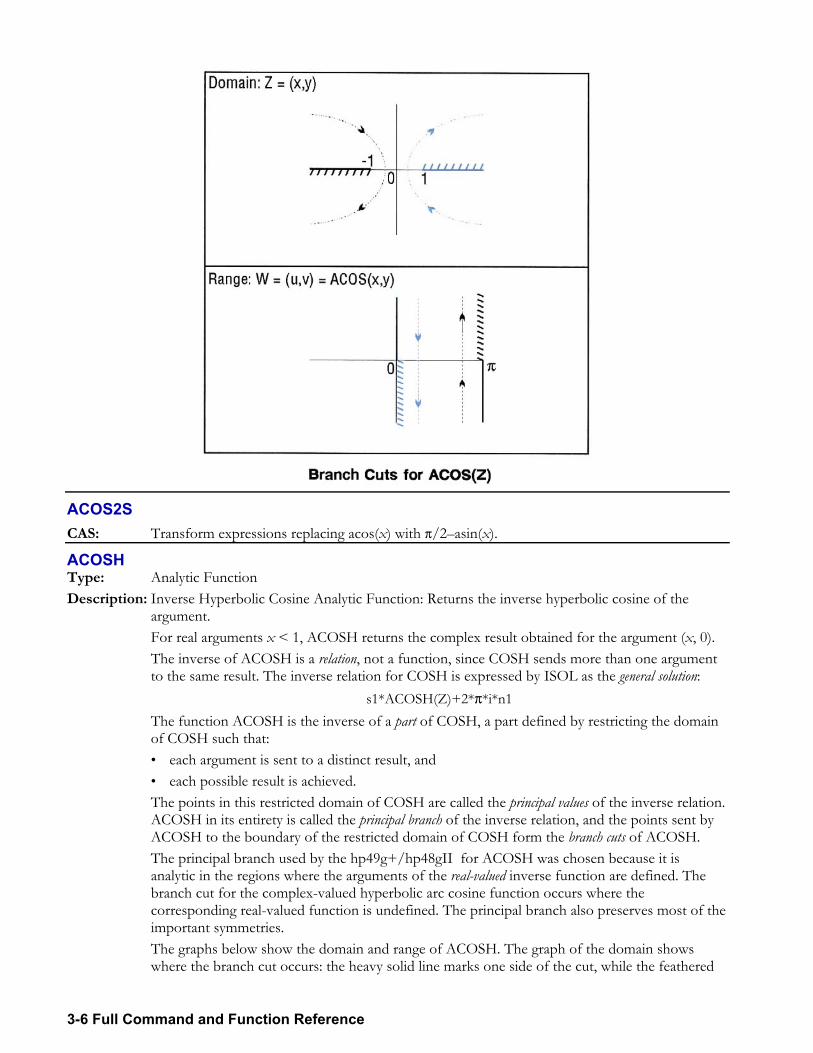
3-6 Full Command and Function Reference
ACOS2S CAS: Transform expressions replacing acos(x) with π/2asin(x).
ACOSH Type: Analytic Function Description: Inverse Hyperbolic Cosine Analytic Function: Returns the inverse hyperbolic cosine of the
argument. For real arguments x < 1, ACOSH returns the complex result obtained for the argument (x, 0). The inverse of ACOSH is a relation, not a function, since COSH sends more than one argument
to the same result. The inverse relation for COSH is expressed by ISOL as the general solution: s1*ACOSH(Z)+2*π*i*n1
The function ACOSH is the inverse of a part of COSH, a part defined by restricting the domain of COSH such that: each argument is sent to a distinct result, and each possible result is achieved.
The points in this restricted domain of COSH are called the principal values of the inverse relation. ACOSH in its entirety is called the principal branch of the inverse relation, and the points sent by ACOSH to the boundary of the restricted domain of COSH form the branch cuts of ACOSH.
The principal branch used by the hp49g+/hp48gII for ACOSH was chosen because it is analytic in the regions where the arguments of the real-valued inverse function are defined. The branch cut for the complex-valued hyperbolic arc cosine function occurs where the corresponding real-valued function is undefined. The principal branch also preserves most of the important symmetries.
The graphs below show the domain and range of ACOSH. The graph of the domain shows where the branch cut occurs: the heavy solid line marks one side of the cut, while the feathered
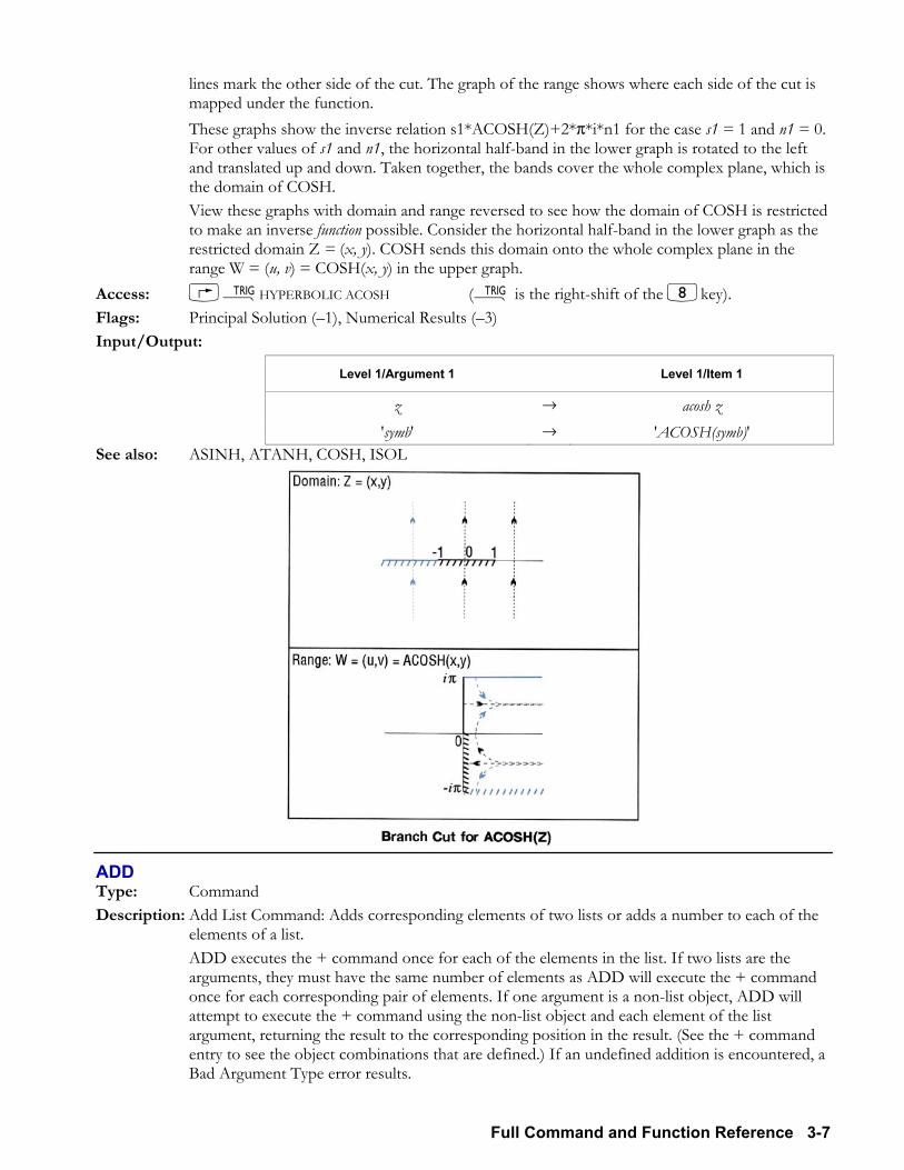
Full Command and Function Reference 3-7
lines mark the other side of the cut. The graph of the range shows where each side of the cut is mapped under the function.
These graphs show the inverse relation s1*ACOSH(Z)+2*π*i*n1 for the case s1 = 1 and n1 = 0. For other values of s1 and n1, the horizontal half-band in the lower graph is rotated to the left and translated up and down. Taken together, the bands cover the whole complex plane, which is the domain of COSH.
View these graphs with domain and range reversed to see how the domain of COSH is restricted to make an inverse function possible. Consider the horizontal half-band in the lower graph as the restricted domain Z = (x, y). COSH sends this domain onto the whole complex plane in the range W = (u, v) = COSH(x, y) in the upper graph.
Access: ÑHYPERBOLIC ACOSH (Ñ is the right-shift of the 8key). Flags: Principal Solution (1), Numerical Results (3) Input/Output:
Level 1/Argument 1 Level 1/Item 1
z → acosh z 'symb' → 'ACOSH(symb)'
See also: ASINH, ATANH, COSH, ISOL
ADD Type: Command Description: Add List Command: Adds corresponding elements of two lists or adds a number to each of the
elements of a list. ADD executes the + command once for each of the elements in the list. If two lists are the
arguments, they must have the same number of elements as ADD will execute the + command once for each corresponding pair of elements. If one argument is a non-list object, ADD will attempt to execute the + command using the non-list object and each element of the list argument, returning the result to the corresponding position in the result. (See the + command entry to see the object combinations that are defined.) If an undefined addition is encountered, a Bad Argument Type error results.
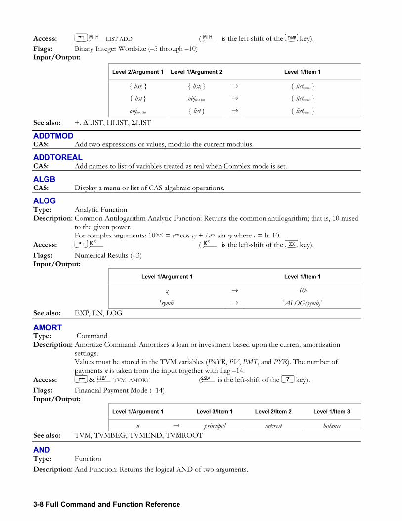
3-8 Full Command and Function Reference
Access: !´LIST ADD ( ´ is the left-shift of the Pkey). Flags: Binary Integer Wordsize (5 through 10) Input/Output:
Level 2/Argument 1 Level 1/Argument 2 Level 1/Item 1
list1 list2 → listresult
list objnon-list → listresult
objnon-list list → listresult See also: +, ∆LIST, ΠLIST, ΣLIST
ADDTMOD CAS: Add two expressions or values, modulo the current modulus.
ADDTOREAL CAS: Add names to list of variables treated as real when Complex mode is set.
ALGB CAS: Display a menu or list of CAS algebraic operations.
ALOG Type: Analytic Function Description: Common Antilogarithm Analytic Function: Returns the common antilogarithm; that is, 10 raised
to the given power. For complex arguments: 10(x,y) = ecx cos cy + i ecx sin cy where c = ln 10. Access: ! (  is the left-shift of the Vkey). Flags: Numerical Results (3) Input/Output:
Level 1/Argument 1 Level 1/Item 1
z → 10z
'symb' → 'ALOG(symb)' See also: EXP, LN, LOG
AMORT Type: Command Description: Amortize Command: Amortizes a loan or investment based upon the current amortization
settings. Values must be stored in the TVM variables (I%YR, PV, PMT, and PYR). The number of
payments n is taken from the input together with flag 14. Access: @& ÎTVM AMORT (Îis the left-shift of the 7key). Flags: Financial Payment Mode (14) Input/Output:
Level 1/Argument 1 Level 3/Item 1 Level 2/Item 2 Level 1/Item 3
n → principal interest balance See also: TVM, TVMBEG, TVMEND, TVMROOT
AND Type: Function Description: And Function: Returns the logical AND of two arguments.
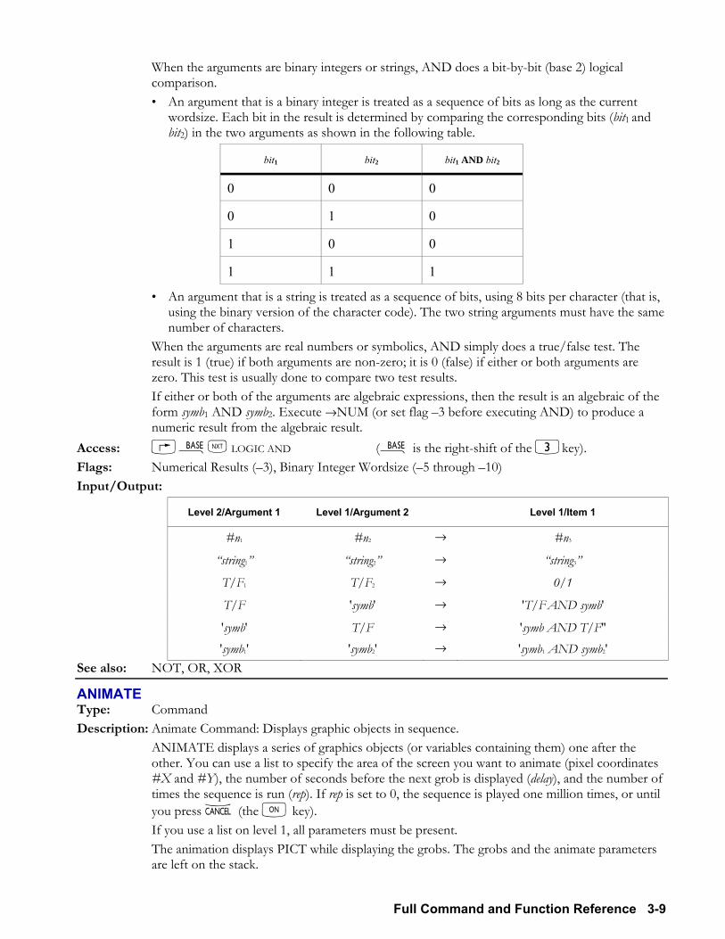
Full Command and Function Reference 3-9
When the arguments are binary integers or strings, AND does a bit-by-bit (base 2) logical comparison. An argument that is a binary integer is treated as a sequence of bits as long as the current
wordsize. Each bit in the result is determined by comparing the corresponding bits (bit1 and bit2) in the two arguments as shown in the following table.
bit1 bit2 bit1 AND bit2
0 0 0
0 1 0
1 0 0
1 1 1
An argument that is a string is treated as a sequence of bits, using 8 bits per character (that is, using the binary version of the character code). The two string arguments must have the same number of characters.
When the arguments are real numbers or symbolics, AND simply does a true/false test. The result is 1 (true) if both arguments are non-zero; it is 0 (false) if either or both arguments are zero. This test is usually done to compare two test results.
If either or both of the arguments are algebraic expressions, then the result is an algebraic of the form symb1 AND symb2. Execute →NUM (or set flag 3 before executing AND) to produce a numeric result from the algebraic result.
Access: ãL LOGIC AND (ã is the right-shift of the 3key). Flags: Numerical Results (3), Binary Integer Wordsize (5 through 10) Input/Output:
Level 2/Argument 1 Level 1/Argument 2 Level 1/Item 1
#n1 #n2 → #n3
string1 string2 → string3
T/F1 T/F2 → 0/1
T/F 'symb' → 'T/F AND symb'
'symb' T/F → 'symb AND T/F'' 'symb1' 'symb2' → 'symb1 AND symb2'
See also: NOT, OR, XOR
ANIMATE Type: Command Description: Animate Command: Displays graphic objects in sequence. ANIMATE displays a series of graphics objects (or variables containing them) one after the
other. You can use a list to specify the area of the screen you want to animate (pixel coordinates #X and #Y), the number of seconds before the next grob is displayed (delay), and the number of times the sequence is run (rep). If rep is set to 0, the sequence is played one million times, or until you press − (the $ key). If you use a list on level 1, all parameters must be present.
The animation displays PICT while displaying the grobs. The grobs and the animate parameters are left on the stack.
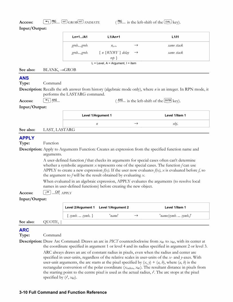
3-10 Full Command and Function Reference
Access: !°LGROBLANIMATE ( °is the left-shift of the Nkey). Input/Output:
Ln+1.../A1 L1/An+1 L1/I1
grobn...grob1 ngrobs → same stack
grobn...grob1 n #X#Y delay rep
→ same stack
L = Level, A = Argument, I = item
See also: BLANK, →GROB
ANS Type: Command Description: Recalls the nth answer from history (algebraic mode only), where n is an integer. In RPN mode, it
performs the LASTARG command. Access: !î ( îis the left-shift of the `key). Input/Output:
Level 1/Argument 1 Level 1/Item 1
n → objn See also: LAST, LASTARG
APPLY Type: Function Description: Apply to Arguments Function: Creates an expression from the specified function name and
arguments. A user-defined function f that checks its arguments for special cases often can't determine
whether a symbolic argument x represents one of the special cases. The function f can use APPLY to create a new expression f(x). If the user now evaluates f(x), x is evaluated before f, so the argument to f will be the result obtained by evaluating x.
When evaluated in an algebraic expression, APPLY evaluates the arguments (to resolve local names in user-defined functions) before creating the new object.
Access: µAPPLY Input/Output:
Level 2/Argument 1 Level 1/Argument 2 Level 1/Item 1
symb1 ... symbn 'name' → 'name(symb1 ... symbn)' See also: QUOTE, |
ARC Type: Command Description: Draw Arc Command: Draws an arc in PICT counterclockwise from xθ1 to xθ2, with its center at
the coordinate specified in argument 1 or level 4 and its radius specified in argument 2 or level 3. ARC always draws an arc of constant radius in pixels, even when the radius and center are
specified in user-units, regardless of the relative scales in user-units of the x- and y-axes. With user-unit arguments, the arc starts at the pixel specified by (x, y) + (a, b), where (a, b) is the rectangular conversion of the polar coordinate (xradius, xθ1). The resultant distance in pixels from the starting point to the centre pixel is used as the actual radius, r'. The arc stops at the pixel specified by (r', xθ2).
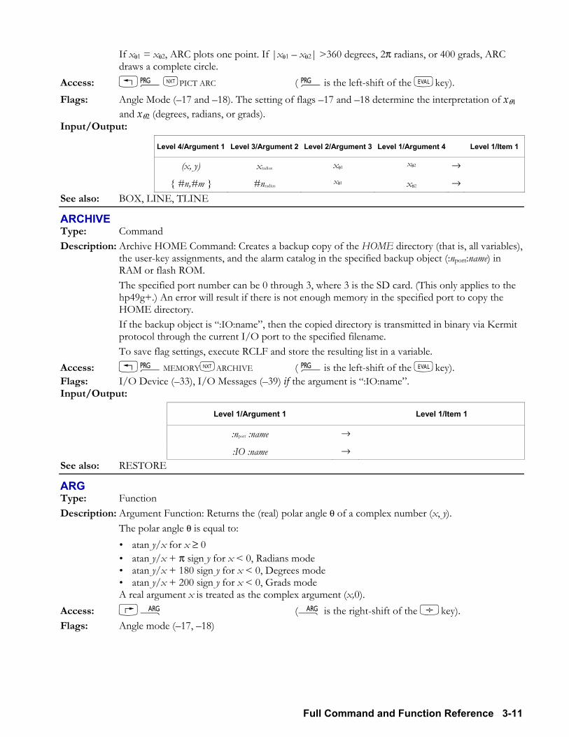
Full Command and Function Reference 3-11
If xθ1 = xθ2, ARC plots one point. If |xθ1 xθ2| >360 degrees, 2π radians, or 400 grads, ARC draws a complete circle.
Access: !°LPICT ARC ( °is the left-shift of the Nkey). Flags: Angle Mode (17 and 18). The setting of flags 17 and 18 determine the interpretation of xθ1
and xθ2 (degrees, radians, or grads). Input/Output:
Level 4/Argument 1 Level 3/Argument 2 Level 2/Argument 3 Level 1/Argument 4 Level 1/Item 1
(x, y) xradius xθ1 xθ2 →
#n,#m #nradius xθ1 xθ2 → See also: BOX, LINE, TLINE
ARCHIVE Type: Command Description: Archive HOME Command: Creates a backup copy of the HOME directory (that is, all variables),
the user-key assignments, and the alarm catalog in the specified backup object (:nport:name) in RAM or flash ROM.
The specified port number can be 0 through 3, where 3 is the SD card. (This only applies to the hp49g+.) An error will result if there is not enough memory in the specified port to copy the HOME directory.
If the backup object is :IO:name, then the copied directory is transmitted in binary via Kermit protocol through the current I/O port to the specified filename.
To save flag settings, execute RCLF and store the resulting list in a variable. Access: !°MEMORYLARCHIVE ( °is the left-shift of the Nkey). Flags: I/O Device (33), I/O Messages (39) if the argument is :IO:name. Input/Output:
Level 1/Argument 1 Level 1/Item 1
:nport :name →
:IO :name → See also: RESTORE
ARG Type: Function Description: Argument Function: Returns the (real) polar angle θ of a complex number (x, y). The polar angle θ is equal to:
atan y/x for x ≥ 0 atan y/x + π sign y for x < 0, Radians mode atan y/x + 180 sign y for x < 0, Degrees mode atan y/x + 200 sign y for x < 0, Grads mode
A real argument x is treated as the complex argument (x,0). Access: Ë (Ë is the right-shift of the /key). Flags: Angle mode (17, 18)
3-12 Full Command and Function Reference
Input/Output:
Level 1/Argument 1 Level 1/Item 1
(x, y) → θ 'symb' → 'ARG(symb)'
See also: ATAN
ARIT CAS: Display a menu or list showing CAS submenus for arithmetical operations
ARRY→ Type: Command Description: Array to Stack Command: Takes an array and returns its elements as separate real or complex
numbers. Also returns a list of the dimensions of the array. If the argument is an n-element vector, the first element is returned to level n + 1 (not level nm +
1), and the nth element to level 2. Access: µ ARRY→ Input/Output:
Level 1/Argument 1 Lnm+1/A1 ... L2/Anm Level1/Itemnm+1
[ vector ] → z1 ... zn nelement
[[ matrix ]] → z11 ... znm nrow mcol L = Level; I = item
See also: →ARRY, DTAG, EQ→, LIST→, OBJ→, STR→
→ARRY Type: Command Description: Stack to Array Command: Returns a vector of n real or complex elements or a matrix of n × m
real or complex elements. The elements of the result array should be entered in row order. If one or more of the elements
is a complex number, the result array will be complex. Access: !°TYPE →ARRY ( °is the left-shift of the Nkey). Input/Output:
Levelnm+1/Argument1 Level2/Argumentnm Level1/Argumentnm+1 Level1/Item1
z1 zn nelement → [ vector ]
z1 1 zn m nrow, mcol → [[ matrix ]] See also: ARRY→, LIST→, →LIST, OBJ→, STR→, →TAG, →UNIT
ASIN Type: Analytic Function Description: Arc Sine Analytic Function: Returns the value of the angle having the given sine. For a real argument x in the domain 1 ≤ x ≤ 1, the result ranges from 90 to +90 degrees (π/2
to +π/2 radians; 100 to +100 grads). A real argument outside of this domain is converted to a complex argument z = x + 0i, and the
result is complex.
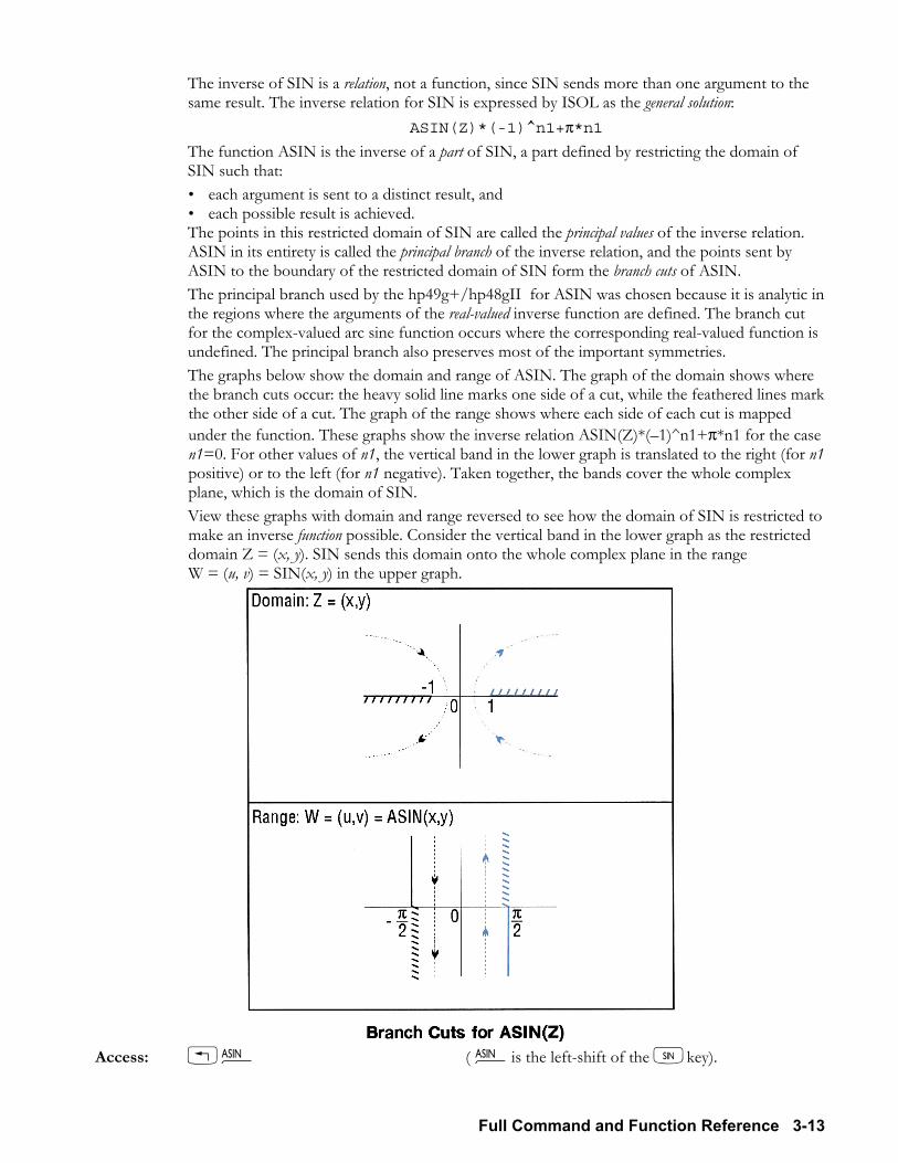
Full Command and Function Reference 3-13
The inverse of SIN is a relation, not a function, since SIN sends more than one argument to the same result. The inverse relation for SIN is expressed by ISOL as the general solution:
ASIN(Z)*(-1)^n1+π*n1 The function ASIN is the inverse of a part of SIN, a part defined by restricting the domain of
SIN such that: each argument is sent to a distinct result, and each possible result is achieved.
The points in this restricted domain of SIN are called the principal values of the inverse relation. ASIN in its entirety is called the principal branch of the inverse relation, and the points sent by ASIN to the boundary of the restricted domain of SIN form the branch cuts of ASIN.
The principal branch used by the hp49g+/hp48gII for ASIN was chosen because it is analytic in the regions where the arguments of the real-valued inverse function are defined. The branch cut for the complex-valued arc sine function occurs where the corresponding real-valued function is undefined. The principal branch also preserves most of the important symmetries.
The graphs below show the domain and range of ASIN. The graph of the domain shows where the branch cuts occur: the heavy solid line marks one side of a cut, while the feathered lines mark the other side of a cut. The graph of the range shows where each side of each cut is mapped under the function. These graphs show the inverse relation ASIN(Z)*(1)^n1+π*n1 for the case n1=0. For other values of n1, the vertical band in the lower graph is translated to the right (for n1 positive) or to the left (for n1 negative). Taken together, the bands cover the whole complex plane, which is the domain of SIN.
View these graphs with domain and range reversed to see how the domain of SIN is restricted to make an inverse function possible. Consider the vertical band in the lower graph as the restricted domain Z = (x, y). SIN sends this domain onto the whole complex plane in the range W = (u, v) = SIN(x, y) in the upper graph.
Access: !¼ ( ¼is the left-shift of the Skey).
3-14 Full Command and Function Reference
Flags: Principal Solution (1), Numerical Results (3), Angle Mode (17, 18) Input/Output:
Level 1/Argument 1 Level 1/Item 1
z → asin z 'symb' → 'ASIN(symb)'
See also: ACOS, ATAN, ISOL, SIN
ASIN2C CAS: Transform expressions replacing asin(x) with π/2acos(x).
ASIN2T CAS: Transform expressions replacing asin(x) with atan(x/√(1-x^2))
ASINH Type: Analytic Function Description: Arc Hyperbolic Sine Analytic Function: Returns the inverse hyperbolic sine of the argument. The inverse of SINH is a relation, not a function, since SINH sends more than one argument to
the same result. The inverse relation for SINH is expressed by ISOL as the general solution: ASINH(Z)*(–1)^n1+π*i*n1
The function ASINH is the inverse of a part of SINH, a part defined by restricting the domain of SINH such that: each argument is sent to a distinct result, and each possible result is achieved.
The points in this restricted domain of SINH are called the principal values of the inverse relation. ASINH in its entirety is called the principal branch of the inverse relation, and the points sent by ASINH to the boundary of the restricted domain of SINH form the branch cuts of ASINH.
The principal branch used by the hp49g+/hp48gII for ASINH was chosen because it is analytic in the regions where the arguments of the real-valued function are defined. The branch cut for the complex-valued ASINH function occurs where the corresponding real-valued function is undefined. The principal branch also preserves most of the important symmetries.
The graph for ASINH can be found from the graph for ASIN (see ASIN) and the relationship asinh z = i asin iz.
Access: ÑHYPERBOLIC ASINH (Ñ is the right-shift of the 8key). Flags: Principal Solution (1), Numerical Results (3) Input/Output:
Level 1/Argument 1 Level 1/Item 1
z → asinh z 'symb' → 'ASINH(symb)'
See also: ACOSH, ATANH, ISOL, SINH
ASN Type: Command Description: Assign Command: Defines a single key on the user keyboard by assigning the given object to the
key xkey, which is specified as rc.pf. The argument xkey is a real number rc.pf specifying the key by its row number r, column number c,
shift plane p and shift-and-hold flag f. A value of f=0 represents a normal shifted key assignment (where the shift is released prior to pressing the key); whereby f=1 corresponds to a shift-and-
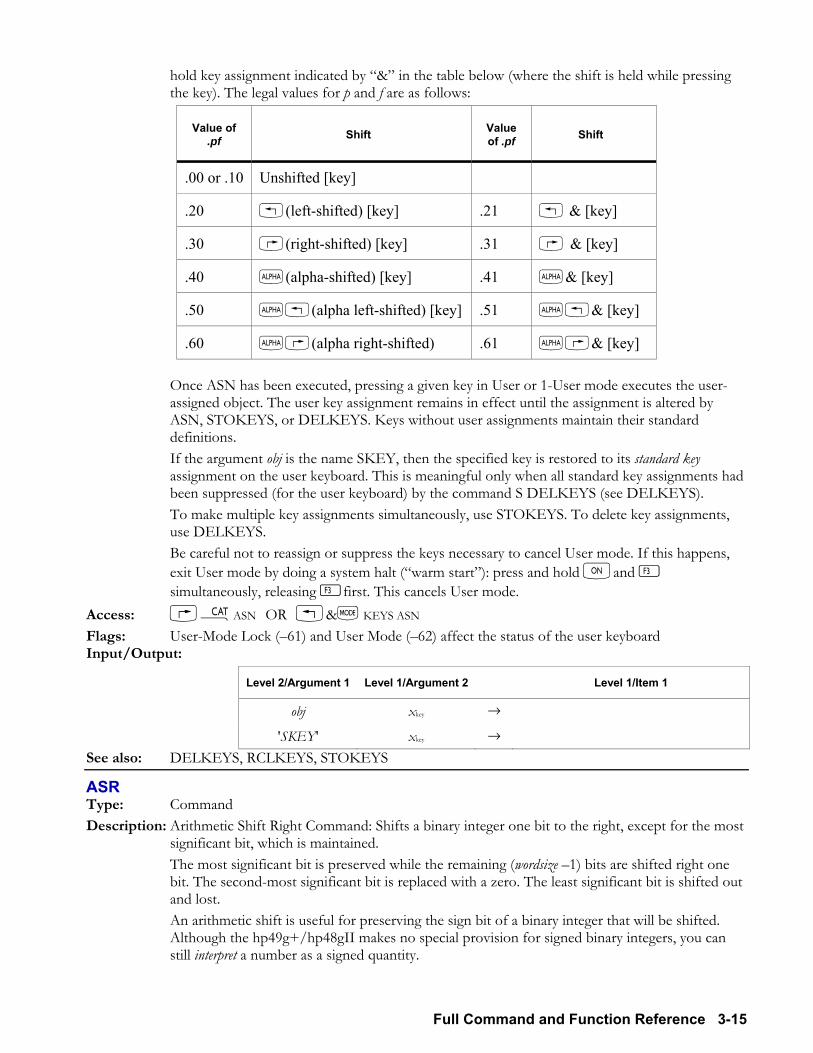
Full Command and Function Reference 3-15
hold key assignment indicated by & in the table below (where the shift is held while pressing the key). The legal values for p and f are as follows:
Value of .pf Shift Value
of .pf Shift
.00 or .10 Unshifted [key]
.20 !(left-shifted) [key] .21 ! & [key]
.30 (right-shifted) [key] .31 & [key]
.40 ~(alpha-shifted) [key] .41 ~& [key]
.50 ~!(alpha left-shifted) [key] .51 ~!& [key]
.60 ~(alpha right-shifted) .61 ~& [key] Once ASN has been executed, pressing a given key in User or 1-User mode executes the user-
assigned object. The user key assignment remains in effect until the assignment is altered by ASN, STOKEYS, or DELKEYS. Keys without user assignments maintain their standard definitions.
If the argument obj is the name SKEY, then the specified key is restored to its standard key assignment on the user keyboard. This is meaningful only when all standard key assignments had been suppressed (for the user keyboard) by the command S DELKEYS (see DELKEYS).
To make multiple key assignments simultaneously, use STOKEYS. To delete key assignments, use DELKEYS.
Be careful not to reassign or suppress the keys necessary to cancel User mode. If this happens, exit User mode by doing a system halt (warm start): press and hold and C simultaneously, releasing Cfirst. This cancels User mode.
Access: µASN OR !&H KEYS ASN Flags: User-Mode Lock (61) and User Mode (62) affect the status of the user keyboard Input/Output:
Level 2/Argument 1 Level 1/Argument 2 Level 1/Item 1
obj xkey →
'SKEY' xkey → See also: DELKEYS, RCLKEYS, STOKEYS
ASR Type: Command Description: Arithmetic Shift Right Command: Shifts a binary integer one bit to the right, except for the most
significant bit, which is maintained. The most significant bit is preserved while the remaining (wordsize 1) bits are shifted right one
bit. The second-most significant bit is replaced with a zero. The least significant bit is shifted out and lost.
An arithmetic shift is useful for preserving the sign bit of a binary integer that will be shifted. Although the hp49g+/hp48gII makes no special provision for signed binary integers, you can still interpret a number as a signed quantity.
3-16 Full Command and Function Reference
Access: ãL BIT ASR ( ãis the right-shift of the 3key). Flags: Binary Integer Wordsize (5 through 10), Binary Integer Base (11, 12) Input/Output:
Level 1/Argument 1 Level 1/Item 1
#n1 → #n2 See also: SL, SLB, SR, SRB
ASSUME CAS: Place assumptions on variables treated by CAS as real when Complex mode is set.
ATAN Type: Analytic Function Description: Arc Tangent Analytic Function: Returns the value of the angle having the given tangent. For a real argument, the result ranges from 90 to +90 degrees (π/2 to +π/2 radians; 100 to
+100 grads). The inverse of TAN is a relation, not a function, since TAN sends more than one argument to the
same result. The inverse relation for TAN is expressed by ISOL as the general solution: ATAN(Z)+π*n1
The function ATAN is the inverse of a part of TAN, a part defined by restricting the domain of TAN such that: each argument is sent to a distinct result, and each possible result is achieved.
The points in this restricted domain of TAN are called the principal values of the inverse relation. ATAN in its entirety is called the principal branch of the inverse relation, and the points sent by ATAN to the boundary of the restricted domain of TAN form the branch cuts of ATAN.
The principal branch used by the hp49g+/hp48gII for ATAN was chosen because it is analytic in the regions where the arguments of the real-valued inverse function are defined. The branch cuts for the complex-valued arc tangent function occur where the corresponding real-valued function is undefined. The principal branch also preserves most of the important symmetries.
The graphs below show the domain and range of ATAN. The graph of the domain shows where the branch cuts occur: the heavy solid line marks one side of a cut, while the feathered lines mark the other side of a cut. The graph of the range shows where each side of each cut is mapped under the function.
These graphs show the inverse relation ATAN(Z)+π*n1 for the case n1 = 0. For other values of n1, the vertical band in the lower graph is translated to the right (for n1 positive) or to the left (for n1 negative). Together, the bands cover the whole complex plane, the domain of TAN.
View these graphs with domain and range reversed to see how the domain of TAN is restricted to make an inverse function possible. Consider the vertical band in the lower graph as the restricted domain Z = (x, y). TAN sends this domain onto the whole complex plane in the range W = (u, v) = TAN(x, y) in the upper graph.
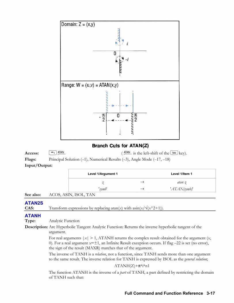
Full Command and Function Reference 3-17
Access: !À ( Àis the left-shift of the Ukey). Flags: Principal Solution (1), Numerical Results (3), Angle Mode (17, 18) Input/Output:
Level 1/Argument 1 Level 1/Item 1
z → atan z 'symb' → 'ATAN(symb)'
See also: ACOS, ASIN, ISOL, TAN
ATAN2S CAS: Transform expressions by replacing atan(x) with asin(x/√(x^2+1)).
ATANH Type: Analytic Function Description: Arc Hyperbolic Tangent Analytic Function: Returns the inverse hyperbolic tangent of the
argument. For real arguments |x| > 1, ATANH returns the complex result obtained for the argument (x,
0). For a real argument x=±1, an Infinite Result exception occurs. If flag 22 is set (no error), the sign of the result (MAXR) matches that of the argument.
The inverse of TANH is a relation, not a function, since TANH sends more than one argument to the same result. The inverse relation for TANH is expressed by ISOL as the general solution;
ATANH(Z)+π*i*n1 The function ATANH is the inverse of a part of TANH, a part defined by restricting the domain
of TANH such that:
3-18 Full Command and Function Reference
each argument is sent to a distinct result, and each possible result is achieved.
The points in this restricted domain of TANH are called the principal values of the inverse relation. ATANH in its entirety is called the principal branch of the inverse relation, and the points sent by ATANH to the boundary of the restricted domain of TANH form the branch cuts of ATANH.
The principal branch used by the hp49g+/hp48gII for ATANH was chosen because it is analytic in the regions where the arguments of the real-valued function are defined. The branch cut for the complex-valued ATANH function occurs where the corresponding real-valued function is undefined. The principal branch also preserves most of the important symmetries.
The graph for ATANH can be found from the graph for ATAN (see ATAN) and the relationship atanh z = i atan iz.
Access: ÑHYPERBOLIC ATAN (Ñ is the right-shift of the 8key). Flags: Principal Solution (1), Numerical Results (3), Infinite Result Exception (22) Input/Output:
Level 1/Argument 1 Level 1/Item 1
z → atanh z 'symb' → 'ATANH(symb)'
See also: ACOSH, ASINH, ISOL, TANH
ATICK Type: Command Description: Axes Tick-Mark Command: Sets the axes tick-mark annotation in the reserved variable PPAR. Given x, ATICK sets the tick-mark annotation to x units on both the x- and the y-axis. For
example, 2 would place tick-marks every 2 units on both axes. Given #n, ATICK sets the tick-mark annotation to #n pixels on both the x- and the y-axis. For
example, #5 would place tick-marks every 5 pixels on both axes. Given x y , ATICK sets the tick-mark unit annotation for each axis individually. For example,
10 3 would mark the x-axis at every multiple of 10 units, and the y-axis at every multiple of 3 units.
Given #n #m ATICK sets the tick-mark pixel annotation for each axis individually. For example, #6 #2 would mark the x-axis every 6 pixels, and the y-axis every 2 pixels.
Access: µATICK Input/Output:
Level 1/Argument 1 Level 1/Item 1
x → #n →
x y → #n #m →
See also: AXES, DRAX
ATTACH Type: Command Description: Attach Library Command: Attaches the library with the specified number to the current
directory. Each library has a unique number. If a port number is specified, it is ignored.
Full Command and Function Reference 3-19
To use a library object, it must be in a port and it must be attached. A library object copied into RAM (such as through the PC Link) must be stored into a port using STO.
Some libraries require you to ATTACH them. You can ascertain whether a library is attached to the current directory by executing LIBS. The number of libraries that can be attached to the HOME directory is limited only by the
available memory. However, only one library at a time can be attached to any other directory. If you attempt to attach a second library to a non-HOME directory, the new library will overwrite the old one.
Access: µATTACH Input/Output:
Level 1/Argument 1 Level 1/Item 1
nlibrary →
:nport :nlibrary → See also: DETACH, LIBS
AUGMENT CAS: Concatenate lists, or vectors, with elements, or create matrices from row vectors.
AUTO Type: Command Description: Autoscale Command: Calculates a y-axis display range, or an x- and y-axis display range. The action of AUTO depends on the plot type as follows:
Plot Type Scaling Action
FUNCTION Samples the equation in EQ at 40 values of the independent variable, equally spaced through the x-axis plotting range, discards points that return ±∞, then sets the y-axis display range to include the maximum, minimum, and origin.
CONIC Sets the y-axis scale equal to the x-axis scale.
POLAR Samples the equation in EQ at 40 values of the independent variable, equally spaced through the plotting range, discards points that return ±∞, then sets both the x- and y-axis display ranges in the same manner as for plot type FUNCTION.
PARAMETRIC Same as POLAR.
TRUTH No action.
BAR Sets the x-axis display range from 0 to the number of elements in ΣDAT, plus 1. Sets the y-range to the minimum and maximum of the elements. The x-axis is always included.
HISTOGRAM Sets the x-axis display range to the minimum and maximum of the elements in ΣDAT. Sets the y-axis display range from 0 to the number of rows in ΣDAT.
3-20 Full Command and Function Reference
Plot Type Scaling Action
SCATTER Sets the x-axis display range to the minimum and maximum of the independent variable column (XCOL) in ΣDAT. Sets the y-axis display range to the minimum and maximum of the dependent variable column (YCOL).
AUTO does not affect 3D plots. AUTO actually calculates a y-axis display range and then expands that range so that the menu
labels do not obscure the resultant plot. AUTO does not draw a plot execute DRAW to do so. Access: µAUTO Input/Output: None See also: DRAW, SCALEH, SCALE, SCLΣ, SCALEW, XRNG, YRNG
AXES Type: Command Description: Axes Command: Specifies the intersection coordinates of the x- and y-axes, tick-mark
annotation, and the labels for the x- and y-axes. This information is stored in the reserved variable PPAR.
The argument for AXES (a complex number or list) is stored as the fifth parameter in the reserved variable PPAR. How the argument is used depends on the type of object it is: If the argument is a complex number, it replaces the current entry in PPAR. If the argument is a list containing any or all of the above variables, only variables that are
specified are affected. atick has the same format as the argument for the ATICK command. This is the variable that is
affected by the ATICK command. The default value for AXES is (0,0). Axes labels are not displayed in PICT until subsequent execution of LABEL. Access: µAXES Input/Output:
Level 1/Argument 1 Level 1/Item 1
(x, y) → (x, y) atick x-axis label y-axis label →
See also: ATICK, DRAW, DRAX, LABEL
AXL CAS: Convert a list to an array, or an array to a list.
AXM CAS: Convert a numeric array to a symbolic matrix, or a symbolic matrix to a numeric array.
AXQ CAS: Convert a square matrix into the associated quadratic form.
BAR Type: Command Description: Bar Plot Type Command: Sets the plot type to BAR.
Full Command and Function Reference 3-21
When the plot type is BAR, the DRAW command plots a bar chart using data from one column of the current statistics matrix (reserved variable ΣDAT). The column to be plotted is specified by the XCOL command, and is stored in the first parameter of the reserved variable ΣPAR. The plotting parameters are specified in the reserved variable PPAR, which has the following form:
(xmin, ymin) (xmax, ymax) indep res axes ptype depend For plot type BAR, the elements of PPAR are used as follows:
(xmin, ymin) is a complex number specifying the lower left corner of PICT (the lower left corner of the display range). The default value is (6.5,3.1) for the hp48gII and (6.5,3.9) for the hp49g+.
(xmax, ymax) is a complex number specifying the upper right corner of PICT (the upper right corner of the display range). The default value is (6.5,3.2) for the hp48gII and (6.5,4.0) for the hp49g+.
indep is either a name specifying a label for the horizontal axis, or a list containing such a name and two numbers, with the smaller of the numbers specifying the horizontal location of the first bar. The default value of indep is X.
res is a real number specifying the bar width in user-unit coordinates, or a binary integer specifying the bar width in pixels. The default value is 0, which specifies a bar width of 1 in user-unit coordinates.
axes is a list containing one or more of the following, in the order listed: a complex number specifying the user-unit coordinates of the plot origin, a list specifying the tick-mark annotation, and two strings specifying labels for the horizontal and vertical axes. The default value is (0,0).
ptype is a command name specifying the plot type. Executing the command BAR places the command name BAR in PPAR.
depend is a name specifying a label for the vertical axis. The default value is Y. A bar is drawn for each element of the column in ΣDAT. Its width is specified by res and its
height is the value of the element. The location of the first bar can be specified by indep; otherwise, the value in (xmin, ymin) is used.
Access: µBAR Input/Output: None See also: CONIC, DIFFEQ, FUNCTION, GRIDMAP, HISTOGRAM, PARAMETRIC,
PARSURFACE, PCONTOUR, POLAR, SCATTER, SLOPEFIELD, TRUTH, WIREFRAME, YSLICE
BARPLOT Type: Command Description: Draw Bar Plot Command: Plots a bar chart of the specified column of the current statistics
matrix (reserved variable ΣDAT). The data column to be plotted is specified by XCOL and is stored as the first parameter in
reserved variable ΣPAR. The default column is 1. Data can be positive or negative, resulting in bars above or below the axis. The y-axis is autoscaled, and the plot type is set to BAR.
When BARPLOT is executed from a program, the resulting plot does not persist unless PICTURE, PVIEW (with an empty list argument), or FREEZE is subsequently executed.
Access: µBARPLOT Input: None Output: A bar chart based on ΣDAT. See also: FREEZE, HISTPLOT, PICTURE, PVIEW, SCATRPLOT, XCOL
3-22 Full Command and Function Reference
BASIS CAS: Determine the basis of a sub-space of the n-space Rn.
BAUD Type: Command Description: Baud Rate Command: Specifies bit-transfer rate. Legal baud rates are 2400, 4800, 9600 (default), 14400, 19200, 38400, 57600 and 115200. Access: µBAUD Input/Output:
Level 1/Argument 1 Level 1/Item 1
nbaudrate → See also: CKSM, PARITY, TRANSIO
BEEP Type: Command Description: Beep Command: Sounds a tone at n hertz for x seconds. The frequency of the tone is subject to the resolution of the built-in tone generator. The
minimum frequency is 1 Hz and the maximum frequency in 15000 Hz. An input that doesnt round to an integer within this range will cause the BEEP command to be skipped. Durations greater than 1200 seconds are automatically changed to 1200 seconds.
Access: !°LOUT L BEEP ( °is the left-shift of the Nkey). Flags: Error Beep (56) Input/Output:
Level 2/Argument 1 Level 1/Argument 2 Level 1/Item 1
nfrequency xduration →
See also: HALT, INPUT, PROMPT, WAIT
BESTFIT Type: Command Description: Best-Fitting Model Command: Executes LR with each of the four curve fitting models, and
selects the model yielding the largest correlation coefficient. The selected model is stored as the fifth parameter in the reserved variable ΣPAR, and the
associated regression coefficients, intercept and slope, are stored as the third and fourth parameters, respectively.
Access: µBESTFIT Input/Output: None See also: EXPFIT, LINFIT, LOGFIT, LR, PWRFIT
BIN Type: Command Description: Binary Mode Command: Selects binary base for binary integer operations. (The default base is
decimal.) Binary integers require the prefix #. Binary integers entered and returned in binary base
automatically show the suffix b. If the current base is not binary, binary numbers can still be entered by using the suffix b (the numbers are displayed in the current base, however). The current base does not affect the internal representation of binary integers as unsigned binary numbers.
Full Command and Function Reference 3-23
Access: ãBIN ( ãis the right-shift of the 3key). Flags: Binary Integer Wordsize (5 through 10), Binary Integer Base (11, 12) Input/Output: None See also: DEC, HEX, OCT, STWS, RCWS
BINS Type: Command Description: Sort into Frequency Bins Command: Sorts the elements of the independent column (XCOL) of
the current statistics matrix (the reserved variable ΣDAT) into (nbins + 2) bins, where the left edge of bin 1 starts at value xmin and each bin has width xwidth.
BINS returns a matrix containing the frequency of occurrences in each bin, and a 2-element array containing the frequency of occurrences falling below or above the defined range of x-values. The array can be stored into the reserved variable ΣDAT and used to plot a bar histogram of the bin data (for example, by executing BARPLOT).
For each element x in ΣDAT, the nth bin count nfreq bin n is incremented, where:
n f re qb in n IP x xm inxwi dth
-------------------=
for xmin £ x £ xmax, where xmax = xmin + (nbins)(xwidth). Access: µBINS Input/Output:
L3/A1 L2/A2 L1/A3 L2/I1 L1/I2
xmin xwidth nbins → [[ nbin 1 ... nbin n ]] [ nbin L nbin R] L = Level; A = Argument; I = item
See also: BARPLOT, XCOL
BLANK Type: Command Description: Blank Graphics Object Command: Creates a blank graphics object of the specified width and
height. Access: !°LGROB BLANK ( °is the left-shift of the Nkey). Input/Output:
Level 2/Argument 1 Level 1/Argument 2 Level 1/Item 1
#nwidth #mheight → grobblank See also: →GROB, LCD→
BOX Type: Command Operation Description: Box Command: Draws in PICT a box whose opposite corners are defined by the specified pixel
or user-unit coordinates. Access: !°LPICT BOX ( °is the left-shift of the Nkey). Input/Output:
Level 2/Argument 1 Level 1/Argument 2 Level 1/Item 1
#n1 #m1 #n2 #m2 →
(x1, y1) (x2, y2) →
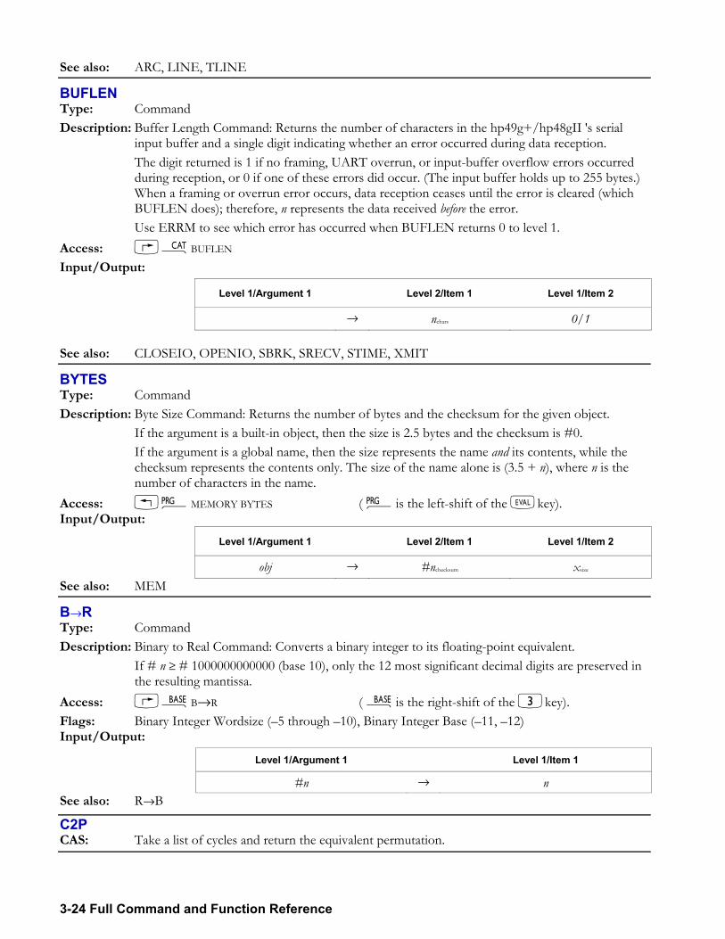
3-24 Full Command and Function Reference
See also: ARC, LINE, TLINE
BUFLEN Type: Command Description: Buffer Length Command: Returns the number of characters in the hp49g+/hp48gII 's serial
input buffer and a single digit indicating whether an error occurred during data reception. The digit returned is 1 if no framing, UART overrun, or input-buffer overflow errors occurred
during reception, or 0 if one of these errors did occur. (The input buffer holds up to 255 bytes.) When a framing or overrun error occurs, data reception ceases until the error is cleared (which BUFLEN does); therefore, n represents the data received before the error.
Use ERRM to see which error has occurred when BUFLEN returns 0 to level 1. Access: µBUFLEN Input/Output:
Level 1/Argument 1 Level 2/Item 1 Level 1/Item 2
→ nchars 0/1 See also: CLOSEIO, OPENIO, SBRK, SRECV, STIME, XMIT
BYTES Type: Command Description: Byte Size Command: Returns the number of bytes and the checksum for the given object. If the argument is a built-in object, then the size is 2.5 bytes and the checksum is #0. If the argument is a global name, then the size represents the name and its contents, while the
checksum represents the contents only. The size of the name alone is (3.5 + n), where n is the number of characters in the name.
Access: !°MEMORY BYTES ( °is the left-shift of the Nkey). Input/Output:
Level 1/Argument 1 Level 2/Item 1 Level 1/Item 2
obj → #nchecksum xsize See also: MEM
B→R Type: Command Description: Binary to Real Command: Converts a binary integer to its floating-point equivalent. If # n ≥ # 1000000000000 (base 10), only the 12 most significant decimal digits are preserved in
the resulting mantissa. Access: ãB→R ( ãis the right-shift of the 3key). Flags: Binary Integer Wordsize (5 through 10), Binary Integer Base (11, 12) Input/Output:
Level 1/Argument 1 Level 1/Item 1
#n → n See also: R→B
C2P CAS: Take a list of cycles and return the equivalent permutation.
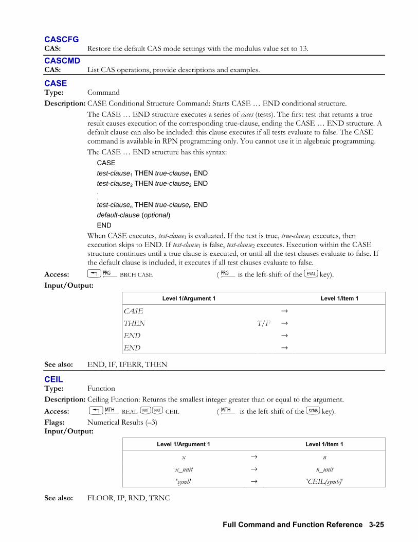
Full Command and Function Reference 3-25
CASCFG CAS: Restore the default CAS mode settings with the modulus value set to 13.
CASCMD CAS: List CAS operations, provide descriptions and examples.
CASE Type: Command Description: CASE Conditional Structure Command: Starts CASE END conditional structure. The CASE END structure executes a series of cases (tests). The first test that returns a true
result causes execution of the corresponding true-clause, ending the CASE END structure. A default clause can also be included: this clause executes if all tests evaluate to false. The CASE command is available in RPN programming only. You cannot use it in algebraic programming.
The CASE END structure has this syntax: CASE test-clause1 THEN true-clause1 END test-clause2 THEN true-clause2 END . . test-clausen THEN true-clausen END default-clause (optional) END
When CASE executes, test-clause1 is evaluated. If the test is true, true-clause1 executes, then execution skips to END. If test-clause1 is false, test-clause2 executes. Execution within the CASE structure continues until a true clause is executed, or until all the test clauses evaluate to false. If the default clause is included, it executes if all test clauses evaluate to false.
Access: !°BRCH CASE ( °is the left-shift of the Nkey). Input/Output:
Level 1/Argument 1 Level 1/Item 1
CASE → THEN T/F → END → END →
See also: END, IF, IFERR, THEN
CEIL Type: Function Description: Ceiling Function: Returns the smallest integer greater than or equal to the argument. Access: !´REAL LL CEIL ( ´ is the left-shift of the Pkey). Flags: Numerical Results (3) Input/Output:
Level 1/Argument 1 Level 1/Item 1
x → n x_unit → n_unit 'symb' → 'CEIL(symb)'
See also: FLOOR, IP, RND, TRNC
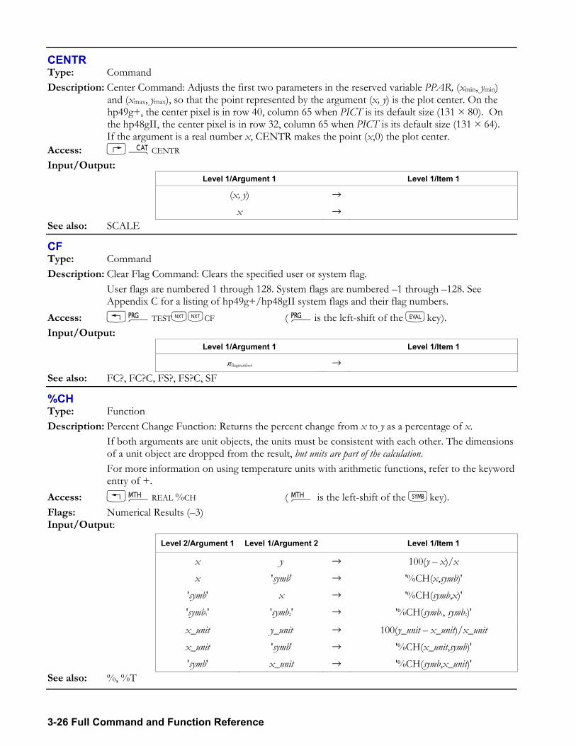
3-26 Full Command and Function Reference
CENTR Type: Command Description: Center Command: Adjusts the first two parameters in the reserved variable PPAR, (xmin, ymin)
and (xmax, ymax), so that the point represented by the argument (x, y) is the plot center. On the hp49g+, the center pixel is in row 40, column 65 when PICT is its default size (131 × 80). On the hp48gII, the center pixel is in row 32, column 65 when PICT is its default size (131 × 64).
If the argument is a real number x, CENTR makes the point (x,0) the plot center. Access: µCENTR Input/Output:
Level 1/Argument 1 Level 1/Item 1
(x, y) → x →
See also: SCALE
CF Type: Command Description: Clear Flag Command: Clears the specified user or system flag. User flags are numbered 1 through 128. System flags are numbered 1 through 128. See
Appendix C for a listing of hp49g+/hp48gII system flags and their flag numbers. Access: !°TESTLLCF ( °is the left-shift of the Nkey). Input/Output:
Level 1/Argument 1 Level 1/Item 1
nflagnumber → See also: FC?, FC?C, FS?, FS?C, SF
%CH Type: Function Description: Percent Change Function: Returns the percent change from x to y as a percentage of x. If both arguments are unit objects, the units must be consistent with each other. The dimensions
of a unit object are dropped from the result, but units are part of the calculation. For more information on using temperature units with arithmetic functions, refer to the keyword
entry of +. Access: !´REAL %CH ( ´ is the left-shift of the Pkey). Flags: Numerical Results (3) Input/Output:
Level 2/Argument 1 Level 1/Argument 2 Level 1/Item 1
x y → 100(y x)/x x 'symb' → '%CH(x,symb)'
'symb' x → '%CH(symb,x)' 'symb1' 'symb2' → '%CH(symb1, symb2)'
x_unit y_unit → 100(y_unit x_unit)/x_unit x_unit 'symb' → '%CH(x_unit,symb)' 'symb' x_unit → '%CH(symb,x_unit)'
See also: %, %T
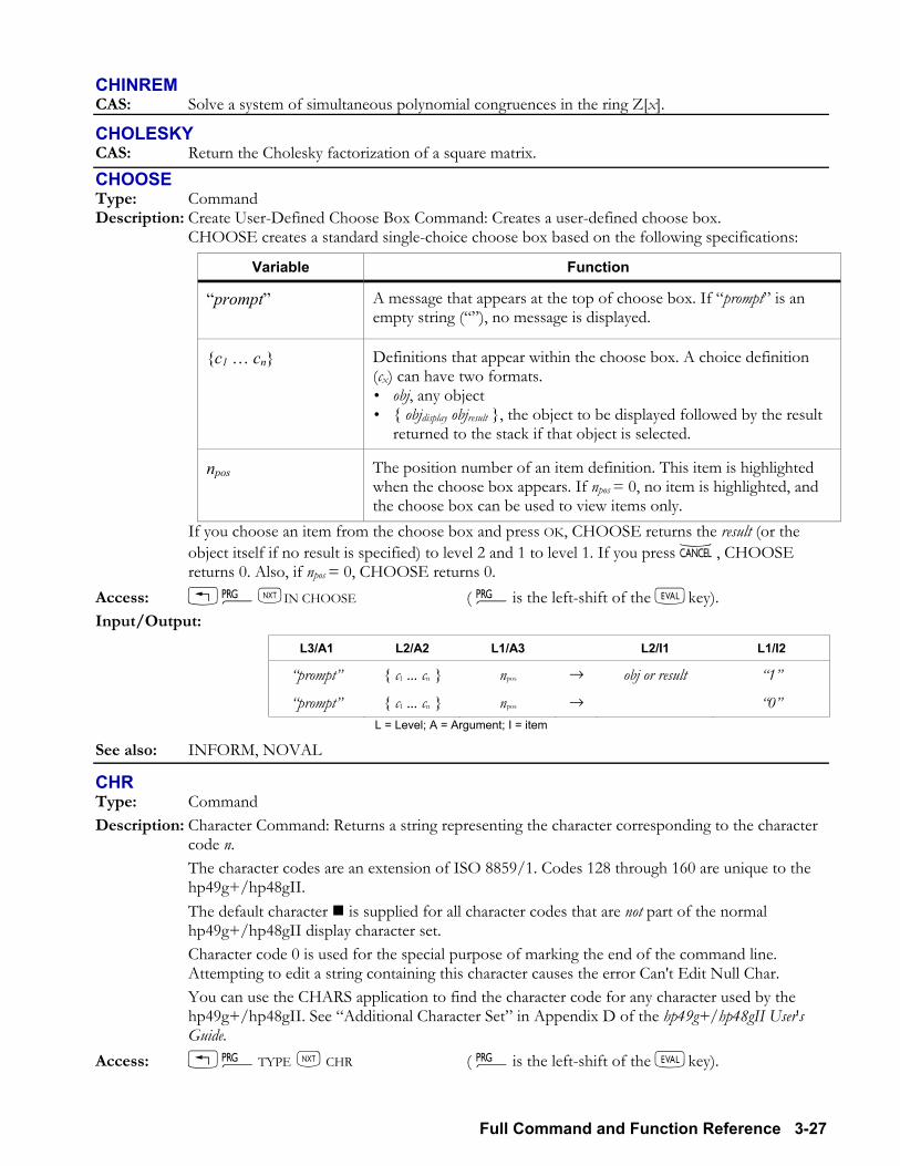
Full Command and Function Reference 3-27
CHINREM CAS: Solve a system of simultaneous polynomial congruences in the ring Z[x].
CHOLESKY CAS: Return the Cholesky factorization of a square matrix.
CHOOSE Type: Command Description: Create User-Defined Choose Box Command: Creates a user-defined choose box. CHOOSE creates a standard single-choice choose box based on the following specifications:
Variable Function
prompt A message that appears at the top of choose box. If prompt is an empty string (), no message is displayed.
c1 cn Definitions that appear within the choose box. A choice definition (cx) can have two formats. obj, any object objdisplay objresult , the object to be displayed followed by the result
returned to the stack if that object is selected.
npos The position number of an item definition. This item is highlighted when the choose box appears. If npos = 0, no item is highlighted, and the choose box can be used to view items only.
If you choose an item from the choose box and press OK, CHOOSE returns the result (or the object itself if no result is specified) to level 2 and 1 to level 1. If you press −, CHOOSE returns 0. Also, if npos = 0, CHOOSE returns 0.
Access: !°LIN CHOOSE ( °is the left-shift of the Nkey). Input/Output:
L3/A1 L2/A2 L1/A3 L2/I1 L1/I2
prompt c1 ... cn npos → obj or result 1
prompt c1 ... cn npos → 0 L = Level; A = Argument; I = item
See also: INFORM, NOVAL
CHR Type: Command Description: Character Command: Returns a string representing the character corresponding to the character
code n. The character codes are an extension of ISO 8859/1. Codes 128 through 160 are unique to the
hp49g+/hp48gII. The default character ! is supplied for all character codes that are not part of the normal
hp49g+/hp48gII display character set. Character code 0 is used for the special purpose of marking the end of the command line.
Attempting to edit a string containing this character causes the error Can't Edit Null Char. You can use the CHARS application to find the character code for any character used by the
hp49g+/hp48gII. See Additional Character Set in Appendix D of the hp49g+/hp48gII User's Guide.
Access: !°TYPE L CHR ( °is the left-shift of the Nkey).
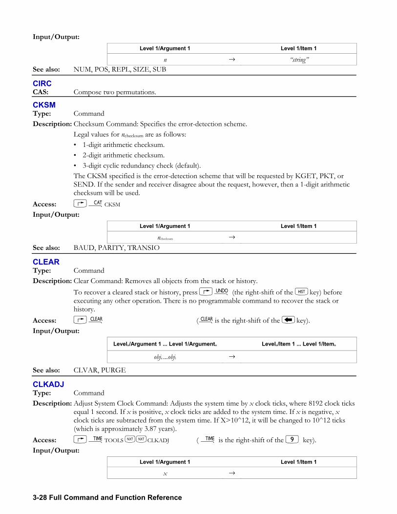
3-28 Full Command and Function Reference
Input/Output: Level 1/Argument 1 Level 1/Item 1
n → string See also: NUM, POS, REPL, SIZE, SUB
CIRC CAS: Compose two permutations.
CKSM Type: Command Description: Checksum Command: Specifies the error-detection scheme. Legal values for nchecksum are as follows:
1-digit arithmetic checksum. 2-digit arithmetic checksum. 3-digit cyclic redundancy check (default).
The CKSM specified is the error-detection scheme that will be requested by KGET, PKT, or SEND. If the sender and receiver disagree about the request, however, then a 1-digit arithmetic checksum will be used.
Access: µCKSM Input/Output:
Level 1/Argument 1 Level 1/Item 1
nchecksum → See also: BAUD, PARITY, TRANSIO
CLEAR Type: Command Description: Clear Command: Removes all objects from the stack or history. To recover a cleared stack or history, press ¯ (the right-shift of the Mkey) before
executing any other operation. There is no programmable command to recover the stack or history.
Access: · (·is the right-shift of the key). Input/Output:
Leveln/Argument 1 ... Level 1/Argumentn Leveln/Item 1 ... Level 1/Itemn
objn ...obj1 →
See also: CLVAR, PURGE
CLKADJ Type: Command Description: Adjust System Clock Command: Adjusts the system time by x clock ticks, where 8192 clock ticks
equal 1 second. If x is positive, x clock ticks are added to the system time. If x is negative, x clock ticks are subtracted from the system time. If X>10^12, it will be changed to 10^12 ticks (which is approximately 3.87 years).
Access: ÓTOOLS LLCLKADJ ( Ó is the right-shift of the 9 key). Input/Output:
Level 1/Argument 1 Level 1/Item 1
x →
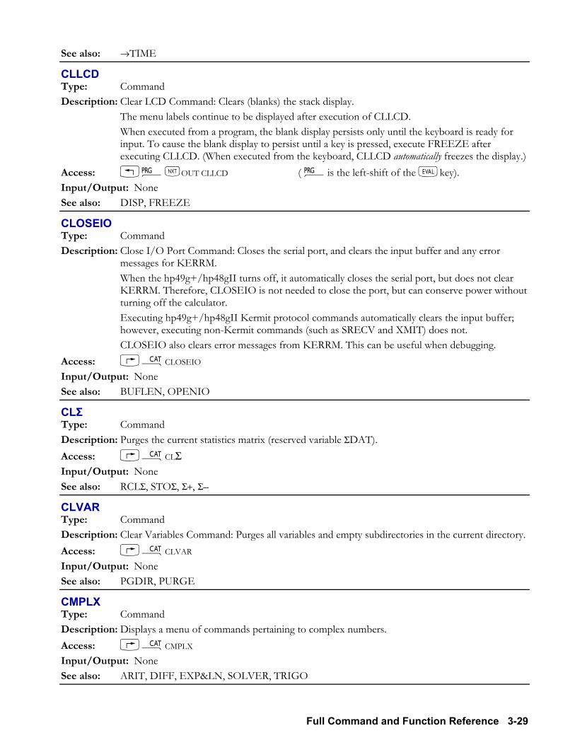
Full Command and Function Reference 3-29
See also: →TIME
CLLCD Type: Command Description: Clear LCD Command: Clears (blanks) the stack display. The menu labels continue to be displayed after execution of CLLCD. When executed from a program, the blank display persists only until the keyboard is ready for
input. To cause the blank display to persist until a key is pressed, execute FREEZE after executing CLLCD. (When executed from the keyboard, CLLCD automatically freezes the display.)
Access: !°LOUT CLLCD ( °is the left-shift of the Nkey). Input/Output: None See also: DISP, FREEZE
CLOSEIO Type: Command Description: Close I/O Port Command: Closes the serial port, and clears the input buffer and any error
messages for KERRM. When the hp49g+/hp48gII turns off, it automatically closes the serial port, but does not clear
KERRM. Therefore, CLOSEIO is not needed to close the port, but can conserve power without turning off the calculator.
Executing hp49g+/hp48gII Kermit protocol commands automatically clears the input buffer; however, executing non-Kermit commands (such as SRECV and XMIT) does not.
CLOSEIO also clears error messages from KERRM. This can be useful when debugging. Access: µCLOSEIO Input/Output: None See also: BUFLEN, OPENIO
CLΣ Type: Command Description: Purges the current statistics matrix (reserved variable ΣDAT). Access: µCLΣ Input/Output: None See also: RCLΣ, STOΣ, Σ+, Σ
CLVAR Type: Command Description: Clear Variables Command: Purges all variables and empty subdirectories in the current directory. Access: µCLVAR Input/Output: None See also: PGDIR, PURGE
CMPLX Type: Command Description: Displays a menu of commands pertaining to complex numbers. Access: µCMPLX Input/Output: None See also: ARIT, DIFF, EXP&LN, SOLVER, TRIGO
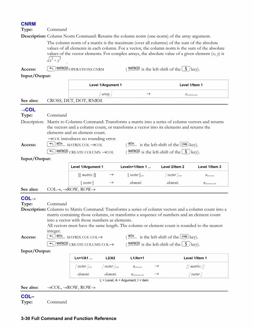
3-30 Full Command and Function Reference
CNRM Type: Command Description: Column Norm Command: Returns the column norm (one-norm) of the array argument. The column norm of a matrix is the maximum (over all columns) of the sum of the absolute
values of all elements in each column. For a vector, the column norm is the sum of the absolute values of the vector elements. For complex arrays, the absolute value of a given element (x, y) is
x2 y2+ . Access: !Ø OPERATIONS CNRM ( Ø is the left-shift of the 5key). Input/Output:
Level 1/Argument 1 Level 1/Item 1
[ array ] → xcolumnnorm See also: CROSS, DET, DOT, RNRM
→COL Type: Command Description: Matrix to Columns Command: Transforms a matrix into a series of column vectors and returns
the vectors and a column count, or transforms a vector into its elements and returns the elements and an element count.
→COL introduces no rounding error. Access: !´MATRIX COL →COL ( ´ is the left-shift of the Pkey). !Ø CREATE COLUMN →COL ( Ø is the left-shift of the 5key). Input/Output:
Level 1/Argument 1 Leveln+1/Item 1 ... Level 2/Item 2 Level 1/Item 3
[[ matrix ]] → [ vector ]col1 [ vector ]coln ncolcount
[ vector ] → element1 elementn nelementcount See also: COL→, →ROW, ROW→
COL→ Type: Command Description: Columns to Matrix Command: Transforms a series of column vectors and a column count into a
matrix containing those columns, or transforms a sequence of numbers and an element count into a vector with those numbers as elements.
All vectors must have the same length. The column or element count is rounded to the nearest integer.
Access: !´MATRIX COL COL→ ( ´ is the left-shift of the Pkey). !Ø CREATE COLUMN COL→ ( Ø is the left-shift of the 5key). Input/Output:
Ln+1/A1 ... L2/A2 L1/An+1 Level 1/Item 1
[ vector ]col1 [ vector ]coln ncolcount → [[ matrix ]]
element1 elementn nelementcount → [ vector ] L = Level; A = Argument; I = item
See also: →COL, →ROW, ROW→
COL Type: Command
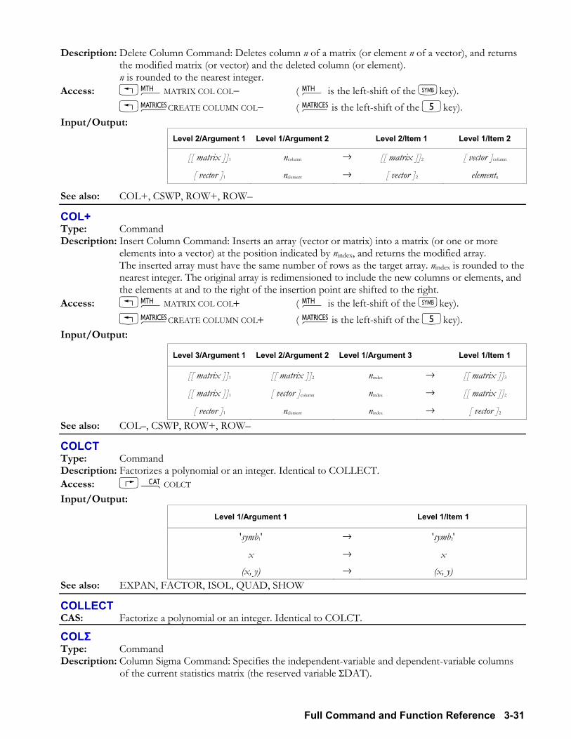
Full Command and Function Reference 3-31
Description: Delete Column Command: Deletes column n of a matrix (or element n of a vector), and returns the modified matrix (or vector) and the deleted column (or element).
n is rounded to the nearest integer. Access: !´MATRIX COL COL− ( ´ is the left-shift of the Pkey). !Ø CREATE COLUMN COL− ( Ø is the left-shift of the 5key). Input/Output:
Level 2/Argument 1 Level 1/Argument 2 Level 2/Item 1 Level 1/Item 2
[[ matrix ]]1 ncolumn → [[ matrix ]]2 [ vector ]column
[ vector ]1 nelement → [ vector ]2 elementn
See also: COL+, CSWP, ROW+, ROW
COL+ Type: Command Description: Insert Column Command: Inserts an array (vector or matrix) into a matrix (or one or more
elements into a vector) at the position indicated by nindex, and returns the modified array. The inserted array must have the same number of rows as the target array. nindex is rounded to the
nearest integer. The original array is redimensioned to include the new columns or elements, and the elements at and to the right of the insertion point are shifted to the right.
Access: !´MATRIX COL COL+ ( ´ is the left-shift of the Pkey). !Ø CREATE COLUMN COL+ ( Ø is the left-shift of the 5key). Input/Output:
Level 3/Argument 1 Level 2/Argument 2 Level 1/Argument 3 Level 1/Item 1
[[ matrix ]]1 [[ matrix ]]2 nindex → [[ matrix ]]3
[[ matrix ]]1 [ vector ]column nindex → [[ matrix ]]2
[ vector ]1 nelement nindex → [ vector ]2 See also: COL, CSWP, ROW+, ROW
COLCT Type: Command Description: Factorizes a polynomial or an integer. Identical to COLLECT. Access: µCOLCT Input/Output:
Level 1/Argument 1 Level 1/Item 1
'symb1' → 'symb2'
x → x (x, y) → (x, y)
See also: EXPAN, FACTOR, ISOL, QUAD, SHOW
COLLECT CAS: Factorize a polynomial or an integer. Identical to COLCT.
COLΣ Type: Command Description: Column Sigma Command: Specifies the independent-variable and dependent-variable columns
of the current statistics matrix (the reserved variable ΣDAT).
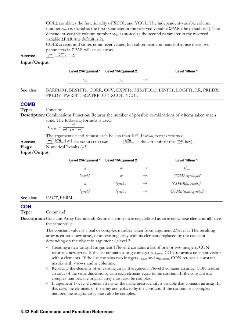
3-32 Full Command and Function Reference
COLΣ combines the functionality of XCOL and YCOL. The independent-variable column number xxcol is stored as the first parameter in the reserved variable ΣPAR (the default is 1). The dependent-variable column number xycol is stored as the second parameter in the reserved variable ΣPAR (the default is 2).
COLΣ accepts and stores noninteger values, but subsequent commands that use these two parameters in ΣPAR will cause errors.
Access: µCOLΣ Input/Output:
Level 2/Argument 1 Level 1/Argument 2 Level 1/Item 1
xcol ycol → See also: BARPLOT, BESTFIT, CORR, COV, EXPFIT, HISTPLOT, LINFIT, LOGFIT, LR, PREDX,
PREDY, PWRFIT, SCATRPLOT, XCOL, YCOL
COMB Type: Function Description: Combinations Function: Returns the number of possible combinations of n items taken m at a
time. The following formula is used:
Cn m,
n!m! n m( )!⋅-------------------------------=
The arguments n and m must each be less than 1012. If n<m, zero is returned. Access: !´L PROBABILITY COMB ( ´ is the left-shift of the Pkey). Flags: Numerical Results (3) Input/Output:
Level 2/Argument 1 Level 1/Argument 2 Level 1/Item 1
n m → Cn;m
'symbn' m → 'COMB(symbn,m)'
n 'symbm' → 'COMB(n, symbm)'
'symbn' 'symbm' → 'COMB(symbn,symbm)' See also: FACT, PERM, !
CON Type: Command Description: Constant Array Command: Returns a constant array, defined as an array whose elements all have
the same value. The constant value is a real or complex number taken from argument 2/level 1. The resulting
array is either a new array, or an existing array with its elements replaced by the constant, depending on the object in argument 1/level 2. Creating a new array: If argument 1/level 2 contains a list of one or two integers, CON
returns a new array. If the list contains a single integer ncolumns, CON returns a constant vector with n elements. If the list contains two integers nrows and mcolumns, CON returns a constant matrix with n rows and m columns.
Replacing the elements of an existing array: If argument 1/level 2 contains an array, CON returns an array of the same dimensions, with each element equal to the constant. If the constant is a complex number, the original array must also be complex.
If argument 1/level 2 contains a name, the name must identify a variable that contains an array. In this case, the elements of the array are replaced by the constant. If the constant is a complex number, the original array must also be complex.
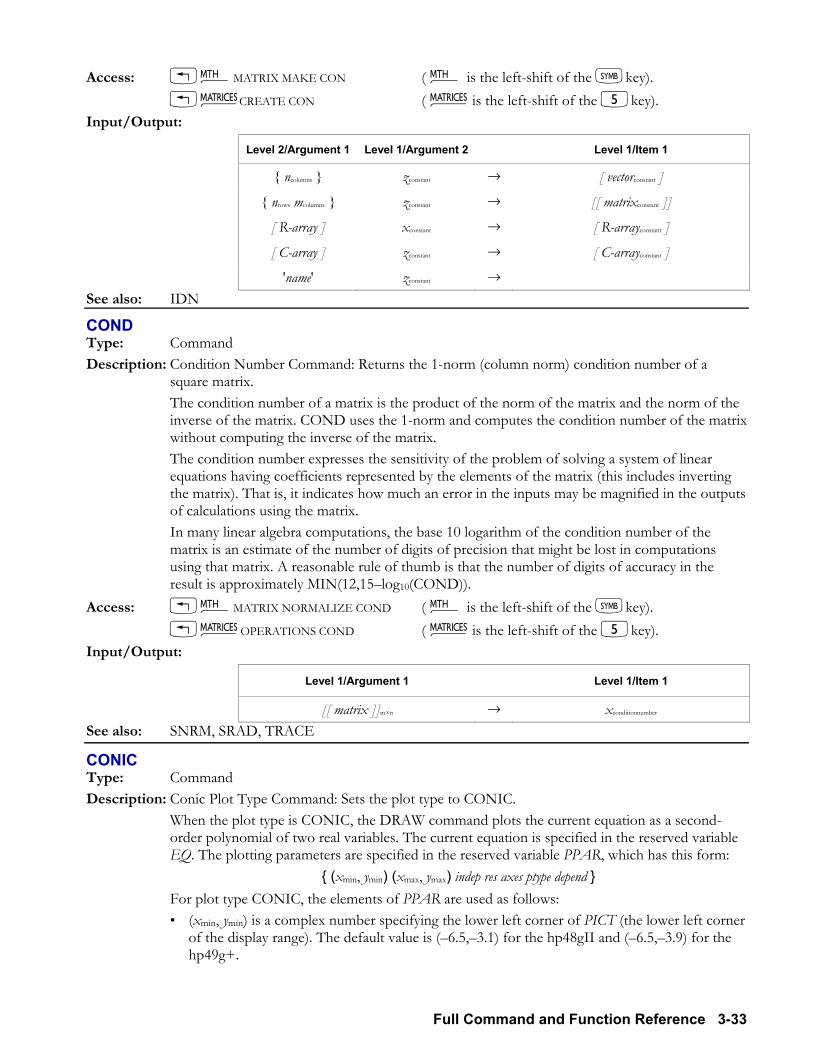
Full Command and Function Reference 3-33
Access: !´MATRIX MAKE CON ( ´ is the left-shift of the Pkey). !Ø CREATE CON ( Ø is the left-shift of the 5key). Input/Output:
Level 2/Argument 1 Level 1/Argument 2 Level 1/Item 1
ncolumns zconstant → [ vectorconstant ]
nrows mcolumns zconstant → [[ matrixconstant ]]
[ R-array ] xconstant → [ R-arrayconstant ]
[ C-array ] zconstant → [ C-arrayconstant ]
'name' zconstant → See also: IDN
COND Type: Command Description: Condition Number Command: Returns the 1-norm (column norm) condition number of a
square matrix. The condition number of a matrix is the product of the norm of the matrix and the norm of the
inverse of the matrix. COND uses the 1-norm and computes the condition number of the matrix without computing the inverse of the matrix.
The condition number expresses the sensitivity of the problem of solving a system of linear equations having coefficients represented by the elements of the matrix (this includes inverting the matrix). That is, it indicates how much an error in the inputs may be magnified in the outputs of calculations using the matrix.
In many linear algebra computations, the base 10 logarithm of the condition number of the matrix is an estimate of the number of digits of precision that might be lost in computations using that matrix. A reasonable rule of thumb is that the number of digits of accuracy in the result is approximately MIN(12,15log10(COND)).
Access: !´MATRIX NORMALIZE COND ( ´ is the left-shift of the Pkey). !Ø OPERATIONS COND ( Ø is the left-shift of the 5key). Input/Output:
Level 1/Argument 1 Level 1/Item 1
[[ matrix ]]m×n → xconditionnumber See also: SNRM, SRAD, TRACE
CONIC Type: Command Description: Conic Plot Type Command: Sets the plot type to CONIC. When the plot type is CONIC, the DRAW command plots the current equation as a second-
order polynomial of two real variables. The current equation is specified in the reserved variable EQ. The plotting parameters are specified in the reserved variable PPAR, which has this form:
(xmin, ymin) (xmax, ymax) indep res axes ptype depend For plot type CONIC, the elements of PPAR are used as follows:
(xmin, ymin) is a complex number specifying the lower left corner of PICT (the lower left corner of the display range). The default value is (6.5,3.1) for the hp48gII and (6.5,3.9) for the hp49g+.
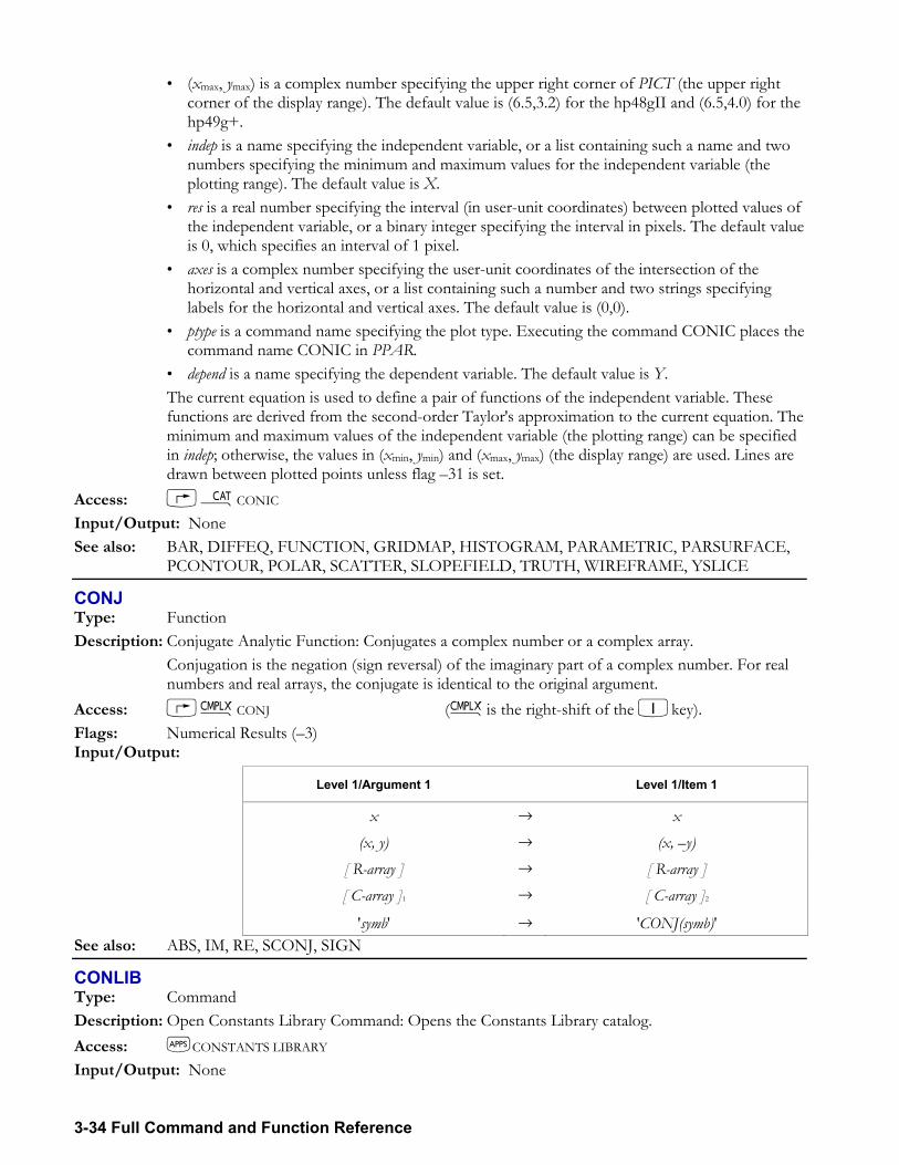
3-34 Full Command and Function Reference
(xmax, ymax) is a complex number specifying the upper right corner of PICT (the upper right corner of the display range). The default value is (6.5,3.2) for the hp48gII and (6.5,4.0) for the hp49g+.
indep is a name specifying the independent variable, or a list containing such a name and two numbers specifying the minimum and maximum values for the independent variable (the plotting range). The default value is X.
res is a real number specifying the interval (in user-unit coordinates) between plotted values of the independent variable, or a binary integer specifying the interval in pixels. The default value is 0, which specifies an interval of 1 pixel.
axes is a complex number specifying the user-unit coordinates of the intersection of the horizontal and vertical axes, or a list containing such a number and two strings specifying labels for the horizontal and vertical axes. The default value is (0,0).
ptype is a command name specifying the plot type. Executing the command CONIC places the command name CONIC in PPAR.
depend is a name specifying the dependent variable. The default value is Y. The current equation is used to define a pair of functions of the independent variable. These
functions are derived from the second-order Taylor's approximation to the current equation. The minimum and maximum values of the independent variable (the plotting range) can be specified in indep; otherwise, the values in (xmin, ymin) and (xmax, ymax) (the display range) are used. Lines are drawn between plotted points unless flag 31 is set.
Access: µCONIC Input/Output: None See also: BAR, DIFFEQ, FUNCTION, GRIDMAP, HISTOGRAM, PARAMETRIC, PARSURFACE,
PCONTOUR, POLAR, SCATTER, SLOPEFIELD, TRUTH, WIREFRAME, YSLICE
CONJ Type: Function Description: Conjugate Analytic Function: Conjugates a complex number or a complex array. Conjugation is the negation (sign reversal) of the imaginary part of a complex number. For real
numbers and real arrays, the conjugate is identical to the original argument. Access: ßCONJ (ßis the right-shift of the 1key). Flags: Numerical Results (3) Input/Output:
Level 1/Argument 1 Level 1/Item 1
x → x (x, y) → (x, y)
[ R-array ] → [ R-array ] [ C-array ]1 → [ C-array ]2
'symb' → 'CONJ(symb)' See also: ABS, IM, RE, SCONJ, SIGN
CONLIB Type: Command Description: Open Constants Library Command: Opens the Constants Library catalog. Access: GCONSTANTS LIBRARY Input/Output: None
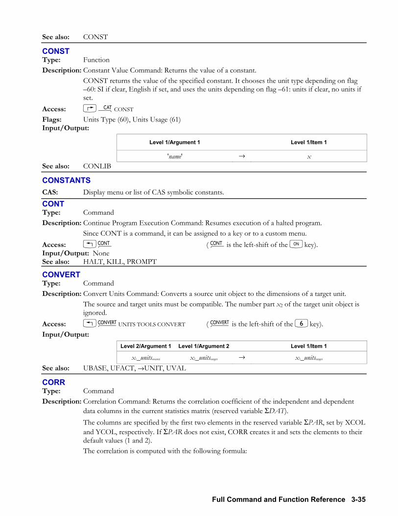
Full Command and Function Reference 3-35
See also: CONST
CONST Type: Function Description: Constant Value Command: Returns the value of a constant. CONST returns the value of the specified constant. It chooses the unit type depending on flag
60: SI if clear, English if set, and uses the units depending on flag 61: units if clear, no units if set.
Access: µCONST Flags: Units Type (60), Units Usage (61) Input/Output:
Level 1/Argument 1 Level 1/Item 1
'name' → x See also: CONLIB
CONSTANTS CAS: Display menu or list of CAS symbolic constants.
CONT Type: Command Description: Continue Program Execution Command: Resumes execution of a halted program. Since CONT is a command, it can be assigned to a key or to a custom menu. Access: !æ ( æis the left-shift of the key). Input/Output: None See also: HALT, KILL, PROMPT
CONVERT Type: Command Description: Convert Units Command: Converts a source unit object to the dimensions of a target unit. The source and target units must be compatible. The number part x2 of the target unit object is
ignored. Access: !Ú UNITS TOOLS CONVERT ( Ú is the left-shift of the 6key). Input/Output:
Level 2/Argument 1 Level 1/Argument 2 Level 1/Item 1
x1_unitssource x2_unitstarget → x3_unitstarget See also: UBASE, UFACT, →UNIT, UVAL
CORR Type: Command Description: Correlation Command: Returns the correlation coefficient of the independent and dependent
data columns in the current statistics matrix (reserved variable ΣDAT). The columns are specified by the first two elements in the reserved variable ΣPAR, set by XCOL
and YCOL, respectively. If ΣPAR does not exist, CORR creates it and sets the elements to their default values (1 and 2).
The correlation is computed with the following formula:
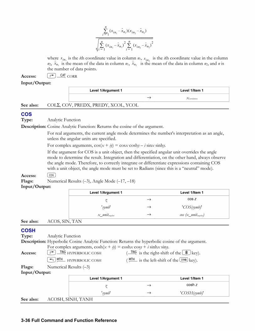
3-36 Full Command and Function Reference
xin1xn1
( ) xin2xn2
( )i 1=
n∑
xin1xn1
( )2
i 1=
n∑ xin2
xn2( )
2
i 1=
n∑
-----------------------------------------------------------------------------------
where is the ith coordinate value in column n1, is the ith coordinate value in the column
n2, is the mean of the data in column n1, is the mean of the data in column n2, and n is the number of data points.
Access: µCORR Input/Output:
Level 1/Argument 1 Level 1/Item 1
→ xcorrelation See also: COLΣ, COV, PREDX, PREDY, XCOL, YCOL
COS Type: Analytic Function Description: Cosine Analytic Function: Returns the cosine of the argument. For real arguments, the current angle mode determines the number's interpretation as an angle,
unless the angular units are specified. For complex arguments, cos(x + iy) = cosx coshy i sinx sinhy. If the argument for COS is a unit object, then the specified angular unit overrides the angle
mode to determine the result. Integration and differentiation, on the other hand, always observe the angle mode. Therefore, to correctly integrate or differentiate expressions containing COS with a unit object, the angle mode must be set to Radians (since this is a neutral mode).
Access: T Flags: Numerical Results (3), Angle Mode (17, 18) Input/Output:
Level 1/Argument 1 Level 1/Item 1
z → cos z
'symb' → 'COS(symb)' x_unitangular → cos (x_unitangular)
See also: ACOS, SIN, TAN
COSH Type: Analytic Function Description: Hyperbolic Cosine Analytic Function: Returns the hyperbolic cosine of the argument. For complex arguments, cosh(x + iy) = coshx cosy + i sinhx siny. Access: ÑHYPERBOLIC COSH (Ñ is the right-shift of the 8key). !´HYPERBOLIC COSH ( ´is the left-shift of the Pkey). Flags: Numerical Results (3) Input/Output:
Level 1/Argument 1 Level 1/Item 1
z → cosh z
'symb' → 'COSH(symb)' See also: ACOSH, SINH, TANH
xin1xin2
xn1xn2
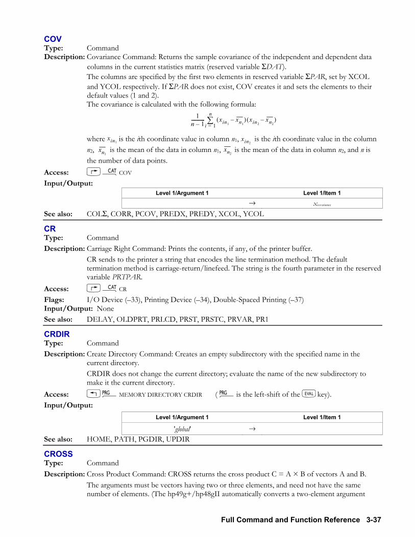
Full Command and Function Reference 3-37
COV Type: Command Description: Covariance Command: Returns the sample covariance of the independent and dependent data
columns in the current statistics matrix (reserved variable ΣDAT). The columns are specified by the first two elements in reserved variable ΣPAR, set by XCOL
and YCOL respectively. If ΣPAR does not exist, COV creates it and sets the elements to their default values (1 and 2).
The covariance is calculated with the following formula:
1n 1------------ xin1
xn1( ) xin2
xn2( )
i 1=
n∑
where is the ith coordinate value in column n1, is the ith coordinate value in the column
n2, is the mean of the data in column n1, is the mean of the data in column n2, and n is the number of data points.
Access: µCOV Input/Output:
Level 1/Argument 1 Level 1/Item 1
→ xcovariance See also: COLΣ, CORR, PCOV, PREDX, PREDY, XCOL, YCOL
CR Type: Command Description: Carriage Right Command: Prints the contents, if any, of the printer buffer. CR sends to the printer a string that encodes the line termination method. The default
termination method is carriage-return/linefeed. The string is the fourth parameter in the reserved variable PRTPAR.
Access: µCR Flags: I/O Device (33), Printing Device (34), Double-Spaced Printing (37) Input/Output: None See also: DELAY, OLDPRT, PRLCD, PRST, PRSTC, PRVAR, PR1
CRDIR Type: Command Description: Create Directory Command: Creates an empty subdirectory with the specified name in the
current directory. CRDIR does not change the current directory; evaluate the name of the new subdirectory to
make it the current directory. Access: !°MEMORY DIRECTORY CRDIR ( °is the left-shift of the Nkey). Input/Output:
Level 1/Argument 1 Level 1/Item 1
'global' →
See also: HOME, PATH, PGDIR, UPDIR
CROSS Type: Command Description: Cross Product Command: CROSS returns the cross product C = A × B of vectors A and B. The arguments must be vectors having two or three elements, and need not have the same
number of elements. (The hp49g+/hp48gII automatically converts a two-element argument
xin1xin2
xn1xn2
3-38 Full Command and Function Reference
[ d1 d2 ] to a three-element argument [ d1 d2 0 ].) Access: !´VECTOR CROSS ( ´ is the left-shift of the Pkey). Input/Output:
Level 2/Argument 1 Level 1/Argument 2 Level 1/Item 1
[ vector ]A [ vector ]B → [ vector ]A × B See also: CNRM, DET, DOT, RNRM
CSWP Type: Command Description: Column Swap Command: Swaps columns i and j of the argument matrix and returns the
modified matrix, or swaps elements i and j of the argument vector and returns the modified vector.
Column numbers are rounded to the nearest integer. Vector arguments are treated as row vectors.
Access: !Ø CREATE COLUMN CSWP ( Ø is the left-shift of the 5key). !´MATRIX COL CSWP ( ´ is the left-shift of the Pkey). Input/Output:
Level 3/Argument 1 Level 2/Argument 2 Level 1/Argument 3 Level 1/Item 1
[[ matrix ]]1 ncolumni ncolumnj → [[ matrix ]]2
[ vector ]1 nelementi nelementj → [ vector ]2 See also: COL+, COL, RSWP
CURL CAS: Return the curl of a three-dimensional vector function.
CYCLOTOMIC CAS: Return the cyclotomic polynomial of order n.
CYLIN Type: Command Description: Cylindrical Mode Command: Sets Cylindrical coordinate mode. CYLIN clears flag 15 and sets flag 16. In Cylindrical mode, vectors are displayed as polar components. Access: !´VECTOR L CYLIN ( ´ is the left-shift of the Pkey). Input/Output: None See also: RECT, SPHERE
C→PX Type: Command Description: Complex to Pixel Command: Converts the specified user-unit coordinates to pixel coordinates. The user-unit coordinates are derived from the (xmin, ymin) and (xmax, ymax) parameters in the
reserved variable PPAR. Access: !°LPICT LC→PX ( °is the left-shift of the Nkey). Input/Output:
Level 1/Argument 1 Level 1/Item 1
(x, y) → #n, #m See also: PX→C
Full Command and Function Reference 3-39
C→R Type: Command Description: Complex to Real Command: Separates the real and imaginary parts of a complex number or
complex array. The result in item 1/level 2 represents the real part of the complex argument. The result in item 2/ level 1 represents the imaginary part of the complex argument.
Access: !°TYPE LC→R ( °is the left-shift of the Nkey). Input/Output:
Level 1/Argument 1 Level 2/Item 1 Level 1/Item 2
(x, y) → x y [ C-array ] → [R-array ]1 [R-array ]2
See also: R→C, RE, IM
DARCY Type: Function Description: Darcy Friction Factor Function: Calculates the Darcy friction factor of certain fluid flows. DARCY calculates the Fanning friction factor and multiplies it by 4. xe/D is the relative roughness
the ratio of the conduit roughness to its diameter. yRe is the Reynolds number. The function uses different computation routines for laminar flow (Re ≤ 2100) and turbulent flow (Re > 2100). xe/D and yRe must be real numbers or unit objects that reduce to dimensionless numbers, and both numbers must be greater than 0.
Access: µ DARCY Input/Output:
Level 2/Argument 1 Level 1/Argument 2 Level 1/Item 1
xe / D yRe → xDarcy See also: FANNING
DATE Type: Command Description: Date Command: Returns the system date. Access: ÓTOOLS DATE (Ó is the right-shift of the 9 key). &9 DATE Flags: Date Format (-42) Input/Output:
Level 1/Argument 1 Level 1/Item 1
→ date See also: DATE+, DDAYS, TIME, TSTR
→DATE Type: Command Description: Set Date Command: Sets the system date to date. date has the form MM.DDYYYY or DD.MMYYYY, depending on the state of flag 42. MM is
month, DD is day, and YYYY is year. If YYYY is not supplied, the current specification for the year is used. The range of allowable dates is January 1, 2000 to December 31, 2090. Inputs between January 1, 1991 and December 31, 1999 are silently rejected by →DATE; no error is reported and the system date is left unchanged.
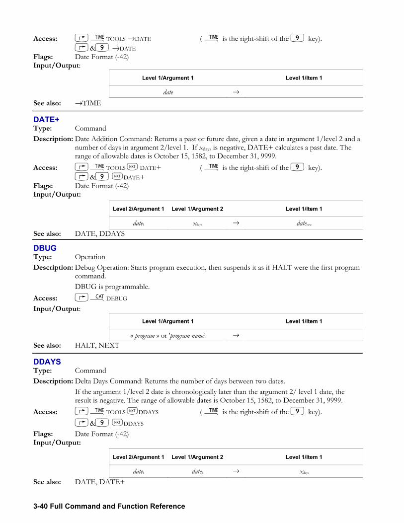
3-40 Full Command and Function Reference
Access: ÓTOOLS →DATE ( Ó is the right-shift of the 9 key). &9 →DATE Flags: Date Format (-42) Input/Output:
Level 1/Argument 1 Level 1/Item 1
date → See also: →TIME
DATE+ Type: Command Description: Date Addition Command: Returns a past or future date, given a date in argument 1/level 2 and a
number of days in argument 2/level 1. If xdays is negative, DATE+ calculates a past date. The range of allowable dates is October 15, 1582, to December 31, 9999.
Access: ÓTOOLS L DATE+ ( Ó is the right-shift of the 9 key). &9 LDATE+ Flags: Date Format (-42) Input/Output:
Level 2/Argument 1 Level 1/Argument 2 Level 1/Item 1
date1 xdays → datenew See also: DATE, DDAYS
DBUG Type: Operation Description: Debug Operation: Starts program execution, then suspends it as if HALT were the first program
command. DBUG is programmable. Access: µDEBUG Input/Output:
Level 1/Argument 1 Level 1/Item 1
« program » or 'program name' → See also: HALT, NEXT
DDAYS Type: Command Description: Delta Days Command: Returns the number of days between two dates. If the argument 1/level 2 date is chronologically later than the argument 2/ level 1 date, the
result is negative. The range of allowable dates is October 15, 1582, to December 31, 9999. Access: ÓTOOLS LDDAYS ( Ó is the right-shift of the 9 key). &9 LDDAYS Flags: Date Format (-42) Input/Output:
Level 2/Argument 1 Level 1/Argument 2 Level 1/Item 1
date1 date2 → xdays See also: DATE, DATE+
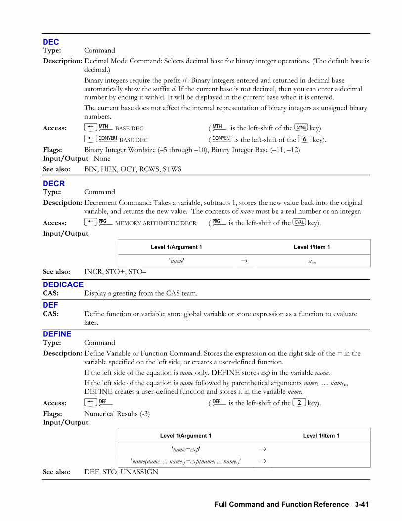
Full Command and Function Reference 3-41
DEC Type: Command Description: Decimal Mode Command: Selects decimal base for binary integer operations. (The default base is
decimal.) Binary integers require the prefix #. Binary integers entered and returned in decimal base
automatically show the suffix d. If the current base is not decimal, then you can enter a decimal number by ending it with d. It will be displayed in the current base when it is entered.
The current base does not affect the internal representation of binary integers as unsigned binary numbers.
Access: !´BASE DEC ( ´ is the left-shift of the Pkey). !Ú BASE DEC ( Ú is the left-shift of the 6key). Flags: Binary Integer Wordsize (5 through 10), Binary Integer Base (11, 12) Input/Output: None See also: BIN, HEX, OCT, RCWS, STWS
DECR Type: Command Description: Decrement Command: Takes a variable, subtracts 1, stores the new value back into the original
variable, and returns the new value. The contents of name must be a real number or an integer. Access: !°MEMORY ARITHMETIC DECR ( °is the left-shift of the Nkey). Input/Output:
Level 1/Argument 1 Level 1/Item 1
'name' → xnew See also: INCR, STO+, STO
DEDICACE CAS: Display a greeting from the CAS team.
DEF CAS: Define function or variable; store global variable or store expression as a function to evaluate
later.
DEFINE Type: Command Description: Define Variable or Function Command: Stores the expression on the right side of the = in the
variable specified on the left side, or creates a user-defined function. If the left side of the equation is name only, DEFINE stores exp in the variable name. If the left side of the equation is name followed by parenthetical arguments name1 namen,
DEFINE creates a user-defined function and stores it in the variable name. Access: !à ( àis the left-shift of the 2key). Flags: Numerical Results (-3) Input/Output:
Level 1/Argument 1 Level 1/Item 1
'name=exp' →
'name(name1 ... namen)=exp(name1 ... namen)' → See also: DEF, STO, UNASSIGN
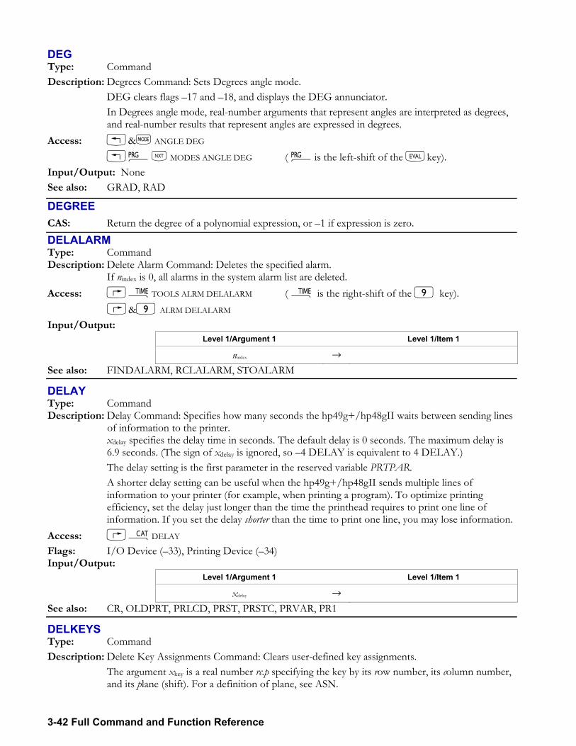
3-42 Full Command and Function Reference
DEG Type: Command Description: Degrees Command: Sets Degrees angle mode. DEG clears flags 17 and 18, and displays the DEG annunciator. In Degrees angle mode, real-number arguments that represent angles are interpreted as degrees,
and real-number results that represent angles are expressed in degrees. Access: !&H ANGLE DEG !°L MODES ANGLE DEG ( °is the left-shift of the Nkey). Input/Output: None See also: GRAD, RAD
DEGREE CAS: Return the degree of a polynomial expression, or 1 if expression is zero.
DELALARM Type: Command Description: Delete Alarm Command: Deletes the specified alarm. If nindex is 0, all alarms in the system alarm list are deleted. Access: ÓTOOLS ALRM DELALARM ( Ó is the right-shift of the 9 key). &9 ALRM DELALARM Input/Output:
Level 1/Argument 1 Level 1/Item 1
nindex → See also: FINDALARM, RCLALARM, STOALARM
DELAY Type: Command Description: Delay Command: Specifies how many seconds the hp49g+/hp48gII waits between sending lines
of information to the printer. xdelay specifies the delay time in seconds. The default delay is 0 seconds. The maximum delay is
6.9 seconds. (The sign of xdelay is ignored, so 4 DELAY is equivalent to 4 DELAY.) The delay setting is the first parameter in the reserved variable PRTPAR. A shorter delay setting can be useful when the hp49g+/hp48gII sends multiple lines of
information to your printer (for example, when printing a program). To optimize printing efficiency, set the delay just longer than the time the printhead requires to print one line of information. If you set the delay shorter than the time to print one line, you may lose information.
Access: µDELAY Flags: I/O Device (33), Printing Device (34) Input/Output:
Level 1/Argument 1 Level 1/Item 1
xdelay → See also: CR, OLDPRT, PRLCD, PRST, PRSTC, PRVAR, PR1
DELKEYS Type: Command Description: Delete Key Assignments Command: Clears user-defined key assignments. The argument xkey is a real number rc.p specifying the key by its row number, its column number,
and its plane (shift). For a definition of plane, see ASN.
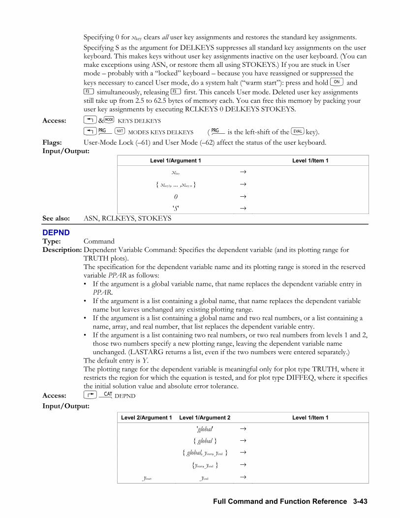
Full Command and Function Reference 3-43
Specifying 0 for xkey clears all user key assignments and restores the standard key assignments. Specifying S as the argument for DELKEYS suppresses all standard key assignments on the user
keyboard. This makes keys without user key assignments inactive on the user keyboard. (You can make exceptions using ASN, or restore them all using STOKEYS.) If you are stuck in User mode probably with a locked keyboard because you have reassigned or suppressed the keys necessary to cancel User mode, do a system halt (warm start): press and hold and C simultaneously, releasing C first. This cancels User mode. Deleted user key assignments still take up from 2.5 to 62.5 bytes of memory each. You can free this memory by packing your user key assignments by executing RCLKEYS 0 DELKEYS STOKEYS.
Access: !&H KEYS DELKEYS !°L MODES KEYS DELKEYS ( °is the left-shift of the Nkey). Flags: User-Mode Lock (61) and User Mode (62) affect the status of the user keyboard. Input/Output:
Level 1/Argument 1 Level 1/Item 1
xkey →
xkey1, ... ,xkey n →
0 → 'S' →
See also: ASN, RCLKEYS, STOKEYS
DEPND Type: Command Description: Dependent Variable Command: Specifies the dependent variable (and its plotting range for
TRUTH plots). The specification for the dependent variable name and its plotting range is stored in the reserved
variable PPAR as follows: If the argument is a global variable name, that name replaces the dependent variable entry in
PPAR. If the argument is a list containing a global name, that name replaces the dependent variable
name but leaves unchanged any existing plotting range. If the argument is a list containing a global name and two real numbers, or a list containing a
name, array, and real number, that list replaces the dependent variable entry. If the argument is a list containing two real numbers, or two real numbers from levels 1 and 2,
those two numbers specify a new plotting range, leaving the dependent variable name unchanged. (LASTARG returns a list, even if the two numbers were entered separately.)
The default entry is Y. The plotting range for the dependent variable is meaningful only for plot type TRUTH, where it
restricts the region for which the equation is tested, and for plot type DIFFEQ, where it specifies the initial solution value and absolute error tolerance.
Access: µDEPND Input/Output:
Level 2/Argument 1 Level 1/Argument 2 Level 1/Item 1
'global' → global → global, ystart, yend →
ystart, yend →
ystart yend →
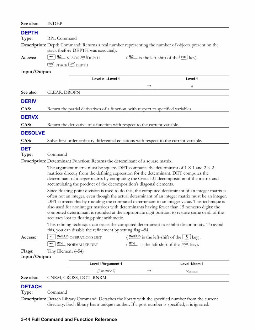
3-44 Full Command and Function Reference
See also: INDEP
DEPTH Type: RPL Command Description: Depth Command: Returns a real number representing the number of objects present on the
stack (before DEPTH was executed). Access: !°STACK LDEPTH ( °is the left-shift of the Nkey). I STACK LDEPTH Input/Output:
Level nLevel 1 Level 1
→ n See also: CLEAR, DROPN
DERIV CAS: Return the partial derivatives of a function, with respect to specified variables.
DERVX CAS: Return the derivative of a function with respect to the current variable.
DESOLVE CAS: Solve first-order ordinary differential equations with respect to the current variable.
DET Type: Command Description: Determinant Function: Returns the determinant of a square matrix. The argument matrix must be square. DET computes the determinant of 1 × 1 and 2 × 2
matrices directly from the defining expression for the determinant. DET computes the determinant of a larger matrix by computing the Crout LU decomposition of the matrix and accumulating the product of the decomposition's diagonal elements.
Since floating-point division is used to do this, the computed determinant of an integer matrix is often not an integer, even though the actual determinant of an integer matrix must be an integer. DET corrects this by rounding the computed determinant to an integer value. This technique is also used for noninteger matrices with determinants having fewer than 15 nonzero digits: the computed determinant is rounded at the appropriate digit position to restore some or all of the accuracy lost to floating-point arithmetic.
This refining technique can cause the computed determinant to exhibit discontinuity. To avoid this, you can disable the refinement by setting flag 54.
Access: !Ø OPERATIONS DET ( Ø is the left-shift of the 5key). !´NORMALIZE DET ( ´ is the left-shift of the Pkey). Flags: Tiny Element (54) Input/Output:
Level 1/Argument 1 Level 1/Item 1
[[ matrix ]] → xdeterminant See also: CNRM, CROSS, DOT, RNRM
DETACH Type: Command Description: Detach Library Command: Detaches the library with the specified number from the current
directory. Each library has a unique number. If a port number is specified, it is ignored.
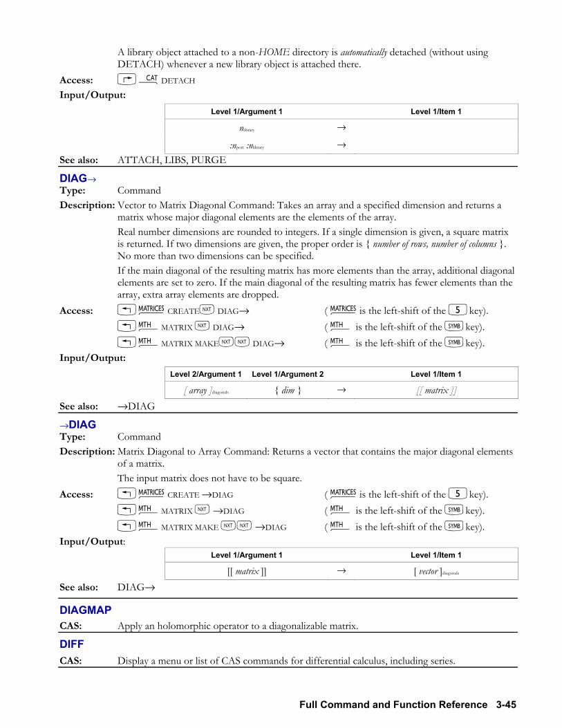
Full Command and Function Reference 3-45
A library object attached to a non-HOME directory is automatically detached (without using DETACH) whenever a new library object is attached there.
Access: µDETACH Input/Output:
Level 1/Argument 1 Level 1/Item 1
nlibrary →
:nport :nlibrary → See also: ATTACH, LIBS, PURGE
DIAG→ Type: Command Description: Vector to Matrix Diagonal Command: Takes an array and a specified dimension and returns a
matrix whose major diagonal elements are the elements of the array. Real number dimensions are rounded to integers. If a single dimension is given, a square matrix
is returned. If two dimensions are given, the proper order is number of rows, number of columns . No more than two dimensions can be specified.
If the main diagonal of the resulting matrix has more elements than the array, additional diagonal elements are set to zero. If the main diagonal of the resulting matrix has fewer elements than the array, extra array elements are dropped.
Access: !Ø CREATEL DIAG→ ( Ø is the left-shift of the 5key). !´MATRIX L DIAG→ ( ´ is the left-shift of the Pkey). !´MATRIX MAKELL DIAG→ ( ´ is the left-shift of the Pkey). Input/Output:
Level 2/Argument 1 Level 1/Argument 2 Level 1/Item 1
[ array ]diagonals dim → [[ matrix ]] See also: →DIAG
→DIAG Type: Command Description: Matrix Diagonal to Array Command: Returns a vector that contains the major diagonal elements
of a matrix. The input matrix does not have to be square. Access: !Ø CREATE →DIAG ( Ø is the left-shift of the 5key). !´MATRIX L →DIAG ( ´ is the left-shift of the Pkey). !´MATRIX MAKE LL →DIAG ( ´ is the left-shift of the Pkey). Input/Output:
Level 1/Argument 1 Level 1/Item 1
[[ matrix ]] → [ vector ]diagonals See also: DIAG→
DIAGMAP CAS: Apply an holomorphic operator to a diagonalizable matrix.
DIFF CAS: Display a menu or list of CAS commands for differential calculus, including series.
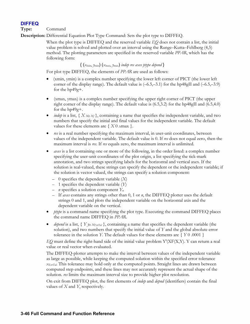
3-46 Full Command and Function Reference
DIFFEQ Type: Command Description: Differential Equation Plot Type Command: Sets the plot type to DIFFEQ. When the plot type is DIFFEQ and the reserved variable EQ does not contain a list, the initial
value problem is solved and plotted over an interval using the RungeKuttaFehlberg (4,5) method. The plotting parameters are specified in the reserved variable PPAR, which has the following form:
(xmin, ymin) (xmax, ymax) indep res axes ptype depend For plot type DIFFEQ, the elements of PPAR are used as follows:
• (xmin, ymin) is a complex number specifying the lower left corner of PICT (the lower left corner of the display range). The default value is (6.5,3.1) for the hp48gII and (6.5,3.9) for the hp49g+.
• (xmax, ymax) is a complex number specifying the upper right corner of PICT (the upper right corner of the display range). The default value is (6.5,3.2) for the hp48gII and (6.5,4.0) for the hp49g+.
• indep is a list, X x0 xf , containing a name that specifies the independent variable, and two numbers that specify the initial and final values for the independent variable. The default values for these elements are X 0 xmax .
• res is a real number specifying the maximum interval, in user-unit coordinates, between values of the independent variable. The default value is 0. If res does not equal zero, then the maximum interval is res. If res equals zero, the maximum interval is unlimited.
• axes is a list containing one or more of the following, in the order listed: a complex number specifying the user-unit coordinates of the plot origin, a list specifying the tick-mark annotation, and two strings specifying labels for the horizontal and vertical axes. If the solution is real-valued, these strings can specify the dependent or the independent variable; if the solution is vector valued, the strings can specify a solution component:
0 specifies the dependent variable (X) 1 specifies the dependent variable (Y) n specifies a solution component Yn If axes contains any strings other than 0, 1 or n, the DIFFEQ plotter uses the default
strings 0 and 1, and plots the independent variable on the horizontal axis and the dependent variable on the vertical.
• ptype is a command name specifying the plot type. Executing the command DIFFEQ places the command name DIFFEQ in PPAR.
• depend is a list, Y y0 xErrTol , containing a name that specifies the dependent variable (the solution), and two numbers that specify the initial value of Y and the global absolute error tolerance in the solution Y. The default values for these elements are Y 0 .0001
EQ must define the right-hand side of the initial value problem Y'(XF(X,Y). Y can return a real value or real vector when evaluated.
The DIFFEQ-plotter attempts to make the interval between values of the independent variable as large as possible, while keeping the computed solution within the specified error tolerance xErrTol. This tolerance may hold only at the computed points. Straight lines are drawn between computed step endpoints, and these lines may not accurately represent the actual shape of the solution. res limits the maximum interval size to provide higher plot resolution.
On exit from DIFFEQ plot, the first elements of indep and depnd (identifiers) contain the final values of X and Y, respectively.
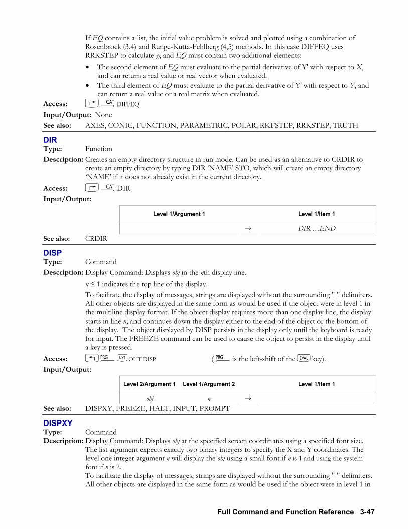
Full Command and Function Reference 3-47
If EQ contains a list, the initial value problem is solved and plotted using a combination of Rosenbrock (3,4) and Runge-Kutta-Fehlberg (4,5) methods. In this case DIFFEQ uses RRKSTEP to calculate yf, and EQ must contain two additional elements: • The second element of EQ must evaluate to the partial derivative of Y' with respect to X,
and can return a real value or real vector when evaluated. • The third element of EQ must evaluate to the partial derivative of Y' with respect to Y, and
can return a real value or a real matrix when evaluated. Access: µDIFFEQ Input/Output: None See also: AXES, CONIC, FUNCTION, PARAMETRIC, POLAR, RKFSTEP, RRKSTEP, TRUTH
DIR Type: Function Description: Creates an empty directory structure in run mode. Can be used as an alternative to CRDIR to
create an empty directory by typing DIR NAME STO, which will create an empty directory NAME if it does not already exist in the current directory.
Access: µDIR Input/Output:
Level 1/Argument 1 Level 1/Item 1
→ DIR END See also: CRDIR
DISP Type: Command Description: Display Command: Displays obj in the nth display line. n ≤ 1 indicates the top line of the display. To facilitate the display of messages, strings are displayed without the surrounding " " delimiters.
All other objects are displayed in the same form as would be used if the object were in level 1 in the multiline display format. If the object display requires more than one display line, the display starts in line n, and continues down the display either to the end of the object or the bottom of the display. The object displayed by DISP persists in the display only until the keyboard is ready for input. The FREEZE command can be used to cause the object to persist in the display until a key is pressed.
Access: !°LOUT DISP ( °is the left-shift of the Nkey). Input/Output:
Level 2/Argument 1 Level 1/Argument 2 Level 1/Item 1
obj n → See also: DISPXY, FREEZE, HALT, INPUT, PROMPT
DISPXY Type: Command Description: Display Command: Displays obj at the specified screen coordinates using a specified font size. The list argument expects exactly two binary integers to specify the X and Y coordinates. The
level one integer argument n will display the obj using a small font if n is 1 and using the system font if n is 2.
To facilitate the display of messages, strings are displayed without the surrounding " " delimiters. All other objects are displayed in the same form as would be used if the object were in level 1 in
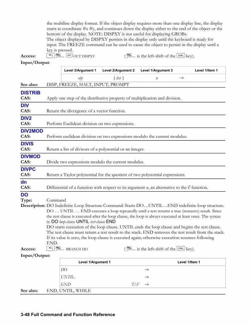
3-48 Full Command and Function Reference
the multiline display format. If the object display requires more than one display line, the display starts at coordinate #x #y, and continues down the display either to the end of the object or the bottom of the display. NOTE: DISPXY is not useful for displaying GROBs.
The object displayed by DISPXY persists in the display only until the keyboard is ready for input. The FREEZE command can be used to cause the object to persist in the display until a key is pressed.
Access: !°LOUT DISPXY ( °is the left-shift of the Nkey). Input/Output:
Level 3/Argument 1 Level 2/Argument 2 Level 1/Argument 3 Level 1/Item 1
obj list n → See also: DISP, FREEZE, HALT, INPUT, PROMPT
DISTRIB CAS: Apply one step of the distributive property of multiplication and division.
DIV CAS: Return the divergence of a vector function.
DIV2 CAS: Perform Euclidean division on two expressions.
DIV2MOD CAS: Perform euclidean division on two expressions modulo the current modulus.
DIVIS CAS: Return a list of divisors of a polynomial or an integer.
DIVMOD CAS: Divide two expressions modulo the current modulus.
DIVPC CAS: Return a Taylor polynomial for the quotient of two polynomial expressions.
dn CAS: Differential of a function with respect to its argument n, an alternative to the ∂ function.
DO Type: Command Description: DO Indefinite Loop Structure Command: Starts DOUNTILEND indefinite loop structure. DO UNTIL END executes a loop repeatedly until a test returns a true (nonzero) result. Since
the test clause is executed after the loop clause, the loop is always executed at least once. The syntax is: DO loop-clause UNTIL test-clause END
DO starts execution of the loop clause. UNTIL ends the loop clause and begins the test clause. The test clause must return a test result to the stack. END removes the test result from the stack. If its value is zero, the loop clause is executed again; otherwise execution resumes following END.
Access: !°BRANCH DO ( °is the left-shift of the Nkey). Input/Output:
Level 1/Argument 1 Level 1/Item 1
DO → UNTIL → END T/F →
See also: END, UNTIL, WHILE
Full Command and Function Reference 3-49
DOERR Type: Command Description: Do Error Command: Executes a user-specified error, causing a program to behave exactly as if
a normal error had occurred during program execution. DOERR causes a program to behave exactly as if a normal error has occurred during program
execution. The error message depends on the argument provided to DOERR: nerror or #nerror display the corresponding built-in error message. "error" displays the contents of the string. (A subsequent execution of ERRM returns "error".
ERRN returns # 70000h.) 0 abandons program execution with an interrupted error message (ERRN = #13Fh). 0 DOERR is equivalent to pressing −.
Access: !°LLERROR DOERR ( °is the left-shift of the Nkey). Input/Output:
Level 1/Argument 1 Level 1/Item 1
nerror →
#nerror →
error → 0 →
See also: ERRM, ERRN, ERR0
DOLIST Type: Command Description: Do to List Command: Applies commands, programs, or user-defined functions to lists. The number of lists, n, can be omitted when the first or level 1 argument is any of the following:
A command. A program containing exactly one command (e.g. « DUP ») A program conforming to the structure of a user-defined function.
The final argument 1 (or level 1 object) can be a local or global name that refers to a program or command.
All lists must be the same length l. The program is executed l times: on the ith iteration, n objects each taken from the ith position in each list are entered on the stack in the same order as in their original lists, and the program is executed. The results from each execution are left on the stack. After the final iteration, any new results are combined into a single list.
Access: !°LIST PROCEDURES DOLIST ( °is the left-shift of the Nkey). Input/Output:
Ln+2/A1 ... L3/An2 L2/An+1 L1/An+2 Level 1/Item 1
list 1 ... list n n « program » → results
list 1 ... list n n command → results
list 1 ... list n n name → results
list 1 ... list n+1 « program » → results
list 1 ... list n+1 command → results
list 1 ... list n+1 name → results L = Level; A = Argument
See also: DOSUBS, ENDSUB, NSUB, STREAM
3-50 Full Command and Function Reference
DOMAIN CAS: List the domain of real numbers for which a function is defined.
DOSUBS Type: Command Description: Do to Sublist Command: Applies a program or command to groups of elements in a list. The real number n can be omitted when the first argument is one of the following:
A command. A user program containing a single command. A program with a user-defined function structure. A global or local name that refers to one of the above.
The first iteration uses elements 1 through n from the list; the second iteration uses elements 2 through n + 1; and so on. In general, the mth iteration uses the elements from the list corresponding to positions m through m + n 1.
During an iteration, the position of the first element used in that iteration is available to the user using the command NSUB, and the number of groups of elements is available using the command ENDSUB. Both of these commands return an Undefined Local Name error if executed when DOSUBS is not active.
DOSUBS returns the Invalid User Function error if the object at level 1/argument 3 is a user program that does not contain only one command and does not have a user-defined function structure. DOSUBS also returns the Wrong Argument Count error if the object at level 1/argument 3 is a command that does not accept 1 to 5 arguments of specific types (DUP, ROT, or →LIST, for example).
Access: !°LIST PROCEDURES DOSUBS ( °is the left-shift of the Nkey). Input/Output:
Level 3/Argument 1 Level 2/Argument 2 Level 1/Argument 3 Level 1/Item 1
list 1 n « program » → list 2
list 1 n command → list 2
list 1 n name → list 2 list 1 « program » → list 2 list 1 command → list 2 list 1 name → list 2
See also: DOLIST, ENDSUB, NSUB, STREAM
DOT Type: Command Description: Dot Product Command: Returns the dot product A•B of two arrays A and B, calculated as the
sum of the products of the corresponding elements of the two arrays. Both arrays must have the same dimensions. Some authorities define the dot product of two complex arrays as the sum of the products of the
conjugated elements of one array with their corresponding elements from the other array. The hp49g+/hp48gII uses the ordinary products without conjugation. If you prefer the alternative definition, apply CONJ to one array before using DOT.
Access: !Ø LVECTOR DOT ( Ø is the left-shift of the 5key). !´VECTOR DOT ( ´ is the left-shift of the Pkey).
Full Command and Function Reference 3-51
Input/Output:
Level 2/Argument 1 Level 1/Argument 2 Level 1/Item 1
[ array A ] [ array B ] → x See also: CNRM, CROSS, DET, RNRM
DRAW Type: Command Operation Description: Draw Plot Command: Plots the mathematical data in the reserved variable EQ or the statistical
data in the reserved variable ΣDAT, using the specified x- and y-axis display ranges. The plot type determines if the data in the reserved variable EQ or the data in the reserved
variable ΣDAT is plotted. DRAW does not erase PICT before plotting; execute ERASE to do so. DRAW does not draw
axes; execute DRAX to do so. When DRAW is executed from a program, the graphics display, which shows the resultant plot,
does not persist unless PICTURE, PVIEW (with an empty list argument), or FREEZE is subsequently executed.
Access: µDRAW Flags: Simultaneous or Sequential Plot (28), Curve Filling (31) Input/Output: None See also: AUTO, AXES, DRAX, ERASE, FREEZE, PICTURE, LABEL, PVIEW
DRAW3DMATRIX Type: Command Description: Draws a 3D plot from the values in a specified matrix. The number of rows indicates the number of units along the x axis, the number of columns
indicates the number of units along the y axis, and the values in the matrix give the magnitudes of the plotted points along the z axis. In other words, the coordinates of a plotted point are (r, c, v) where r is the row number, c the column number and v the value in the corresponding cell of the matrix.
You can limit the points that are plotted by specifing a minimum value (vmin) and a maximum value (vmax). Values in the matrix outside this range are not plotted. If all values are included, the total number of points plotted is r × c.
Once the plot has been drawn, you can rotate it in various ways by pressing the following keys: and rotate the plot around the x axis (in different directions) and rotate the plot around the y axis (in different directions) Iand L rotate the plot around the z axis (in different directions)
Access: µDRAW3DMATRIX Input/Output:
Level 3/Argument 1 Level 2/Argument 2 Level 1/Argument 3 Level 1/Item 1
[[ matrix ]] vmin vmax → See also: FAST3D
DRAX Type: Command Description: Draw Axes Command: Draws axes in PICT.
3-52 Full Command and Function Reference
The coordinates of the axes intersection are specified by AXES. Axes tick-marks are specified in PPAR with the ATICK, or AXES command. DRAX does not draw axes labels; execute LABEL to do so.
Access: µDRAX Input/Output: None See also: AXES, DRAW, LABEL
DROITE CAS: Return an equation for the line through two given points in a plane.
DROP Type: RPL Command Description: Drop Object Command: Removes the level 1 object from the stack. Access: !°STACK DROP ( °is the left-shift of the Nkey). ISTACK DROP in RPN mode executes DROP when no command line is present. Input/Output:
Level 1 Level 1
obj → See also: CLEAR, DROPN, DROP2
DROP2 Type: RPL Command Description: Drop 2 Objects Command: Removes the first two objects from the stack. Access: !°STACK LL DROP2 ( °is the left-shift of the Nkey). ISTACK LL DROP2 Input/Output:
Level 2 Level 1 Level 1
obj1 obj2 → See also: CLEAR, DROP, DROPN
DROPN Type: RPL Command Description: Drop n Objects Command: Removes the first n + 1 objects from the stack (the first n objects
excluding the integer n itself). Access: !°STACK LL DROPN ( °is the left-shift of the Nkey). ISTACK LL DROPN Input/Output:
Leveln+1 ... Level 2 Level 1 Level 1
obj1 ... objn n → See also: CLEAR, DROP, DROP2
DTAG Type: Command Description: Delete Tag Command: DTAG removes all tags (labels) from an object. The leading colon is not shown for readability when the tagged object is on the stack.
Full Command and Function Reference 3-53
DTAG has no effect on an untagged object. Access: !°TYPE LDTAG ( °is the left-shift of the Nkey). Input/Output:
Level 1/Argument 1 Level 1/Item 1
tag:obj → obj See also: LIST→, →TAG
DUP Type: RPL Command Description: Duplicate Object Command: DUP returns a copy of the argument (or the object on level 1). Access: !°STACK DUP ( °is the left-shift of the Nkey). ISTACK DUP ` in RPN mode executes DUP when no command line is present. Input/Output:
Level 1 Level 2 Level 1
obj → obj obj See also: DUPN, DUP2, PICK
DUP2 Type: RPL Command Description: Duplicate 2 Objects Command: DUP2 returns copies of the two objects on levels 1 and 2 of the
stack. Access: !°STACK LL DUP2 ( °is the left-shift of the Nkey). ISTACK LL DUP2 Input/Output:
L2 L1 L4 L3 L2 L1
obj2 obj1 → obj2 obj1 obj2 obj1 L = Level
See also: DUP, DUPN, PICK
DUPDUP Type: RPL Command Description: Duplicates an object twice. Access: !°STACK LL DUPDUP ( °is the left-shift of the Nkey). ISTACK LL DUPDUP Input/Output:
Level 1 Level 3 Level 2 Level 1
obj → obj obj obj See also: DUP, NDUPN, DUPN, DUP2
DUPN Type: RPL Command Description: Duplicate n Objects Command: Takes an integer n from level 1 of the stack, and returns copies
of the objects on stack levels 2 through n + 1.
3-54 Full Command and Function Reference
Access: !°STACK LL DUPN ( °is the left-shift of the Nkey). ISTACK LL DUPN Input/Output:
Li+1 Li L3 L2 L1 Li+n Li+n1 ... L2 L1
obj1 obj2 obji1 obji n → obj1 obj2 ... obji1 obji L = Level
See also: DUP, DUP2, PICK
D→R Type: Function Description: Degrees to Radians Function: Converts a real number representing an angle in degrees to its
equivalent in radians. This function operates independently of the angle mode. Access: !´REAL LL D→R ( ´ is the left-shift of the Pkey). Flags: Numerical Results (3) Input/Output:
Level 1/Argument 1 Level 1/Item 1
x → (π/180)x 'symb' → 'D→R(symb)'
See also: R→D
e Type: Function Description: e Function: Returns the symbolic constant e or its numerical representation, 2.71828182846. The number returned for e is the closest approximation to 12-digit accuracy. For exponentiation,
use the expression EXP(x) rather than e^x, since the function EXP uses a special algorithm to compute the exponential to greater accuracy. Even though the calculator often displays EXP(x) as e^x, its still EXP(x) intenally.
Access: ~!e !´LCONSTANTS e ( ´ is the left-shift of the Pkey). !´LCONSTANTS 2.718281828 ( ´ is the left-shift of the Pkey). Flags: Symbolic Constants (2), Numerical Results (3) Input/Output:
Level 1/Argument 1 Level 1/Item 1
→ 'e' → 2.71828182846
See also: EXP, EXPM, i, LN, LNP1, MAXR, MINR, π
EDIT Type: Command Description: Edit Command: Moves specified object to the command line where it can be edited. Access: ! I!EDIT Input/Output: None See also: EDITB, VISIT
Full Command and Function Reference 3-55
EDITB Type: Command Description: Edit Best Command: Opens the specified object in the most suitable editor. For example, if you
use a matrix as the specified object, the command opens it in Matrix Writer. Access: IEDIT Input/Output: None See also: EDIT, VISIT
EGCD CAS: From polynomials a and b, returns polynomials u, v, and c, where au+bv=c, c is the GCD of a & b.
EGV Type: Command Description: Eigenvalues and Eigenvectors Command: Computes the eigenvalues and right eigenvectors for a
square matrix. The resulting vector EVal contains the computed eigenvalues. The columns of matrix EVec
contain the right eigenvectors corresponding to the elements of vector EVal. The computed results should minimize (within computational precision):
A EVec EVec diag EVal( )⋅⋅n A⋅
-------------------------------------------------------------------------------
where diag (EVal) denotes the n × n diagonal matrix containing the eigenvalues EVal. Access: !Ø LEIGENVECTOR EGV ( Ø is the left-shift of the 5key). !´MATRIX LEGV ( ´ is the left-shift of the Pkey). Input/Output:
Level 1/Argument 1 Level 2/Item 1 Level 1/Item 2
[[matrix ]]A → [[matrix ]]EVec [vector ]EVal See also: EGVL
EGVL Type: Command Description: Eigenvalues Command: Computes the eigenvalues of a square matrix. The resulting vector L contains the computed eigenvalues. Access: !Ø LEIGENVECTOR EGVL ( Ø is the left-shift of the 5key). !´MATRIX LEGVL ( ´ is the left-shift of the Pkey). Input/Output:
Level 1/Argument 1 Level 1/Item 1
[[matrix ]]A → [vector ]EVal See also: EGV
ELSE Type: Command Description: ELSE Command: Starts false clause in conditional or error-trapping structure. See the IF and IFERR keyword entries for more information. Access: !°BRANCH IF ELSE ( °is the left-shift of the Nkey).
3-56 Full Command and Function Reference
Input/Output: None See also: IF, CASE, DO, ELSE, IFERR, REPEAT, THEN, UNTIL, WHILE
END Type: Command Description: END Command: Ends conditional, error-trapping, and indefinite loop structures. See the IF, CASE, IFERR, DO, and WHILE keyword entries for more information. Access: !°BRANCH IF/CASE/DO/WHILE END ( °is the left-shift of the Nkey). Input/Output: None See also: IF, CASE, DO, ELSE, IFERR, REPEAT, THEN, UNTIL, WHILE
ENDSUB Type: Command Description: Ending Sublist Command: Provides a way to access the total number of sublists contained in the
list used by DOSUBS. Returns an Undefined Local Name error if executed when DOSUBS is not active. Access: !°LIST PROCEDURES ENDSUB ( °is the left-shift of the Nkey). Input/Output: None See also: DOSUBS, NSUB
ENG Type: Command Description: Engineering Mode Command: Sets the number display format to engineering mode, which
displays one to three digits to the left of the fraction mark (decimal point) and an exponent that is a multiple of three. The total number of significant digits displayed is n + 1.
Engineering mode uses n + 1 significant digits, where 0 ≤ n ≤ 11. (Values for n outside this range are rounded up or down.) A number is displayed or printed as follows:
(sign) mantissa E (sign) exponent where the mantissa is of the form (nn)n.(n) (with up to 12 digits total) and the exponent has
one to three digits. A number with an exponent of 499 is displayed automatically in scientific mode. Access: ! & H FMT ENG !°L MODES FMT ENG ( °is the left-shift of the Nkey). Input/Output:
Level 1/Argument 1 Level 1/Item 1
n → See also: FIX, SCI, STD
EPSX0 CAS: Replace coefficients in a polynomial, that have an absolute value less than EPS, with 0.
EQNLIB Type: Command Description: Starts the Equation Library application. Access: GEQUATION LIBRARY OR G ` Input/Output: None See also: MSOLVR, SOLVEQN
Full Command and Function Reference 3-57
EQW Type: Command Description: Opens Equation Writer, where you can edit an expression. Puts an object into the Equation Writer. Access: µEQW (Non-programmable access is via when there is an algebraic object on the stack. To start a
new equation when not entering a program object, press ³) Input/Output:
Level 1/Argument 1 Level 1/Item 1
exp1 → exp2 See also: EDIT, EDITB, VISIT, VISITB
EQ→ Type: Command Description: Equation to Stack Command: Separates an equation into its left and right sides. If the argument is an expression, it is treated as an equation whose right side equals zero. Access: !°TYPE LEQ→ ( °is the left-shift of the Nkey). Input/Output:
Level 1/Argument 1 Level 2/Item 1 Level 1/Item 2
'symb1=symb2' → 'symb1' 'symb2'
z → z 0 'name' → 'name' 0
'x_unit' → 'x_unit' 0 'symb' → 'symb' 0
See also: ARRY→, DTAG, LIST→, OBJ→, STR→
ERASE Type: Command Description: Erase PICT Command: Erases PICT, leaving a blank PICT of the same dimensions. Access: µ ERASE Input/Output: None See also: DRAW
ERR0 Type: Command Description: Clear Last Error Number Command: Clears the last error number so that a subsequent execution
of ERRN returns # 0h, and clears the last error message. Access: !°LLERROR ERR0 ( °is the left-shift of the Nkey). Input/Output: None See also: DOERR, ERRM, ERRN
ERRM Type: Command Description: Error Message Command: Returns a string containing the error message of the most recent
calculator error. ERRM returns the string for an error generated by DOERR. If the argument to DOERR was 0,
the string returned by ERRM is Interrupted. Access: !°LL ERROR ERRM ( °is the left-shift of the Nkey).
3-58 Full Command and Function Reference
Input/Output: Level 1/Argument 1 Level 1/Item 1
→ error message See also: DOERR, ERRN, ERR0
ERRN Type: Command Description: Error Number Command: Returns the error number of the most recent calculator error. If the most recent error was generated by DOERR with a string argument, ERRN returns
#70000h. If the most recent error was generated by DOERR with a binary integer argument, ERRN returns that binary integer. (If the most recent error was generated by DOERR with a real number argument, ERRN returns the binary integer conversion of the real number.) The only exceptions to these rules are 0 DOERR and #0 DOERR, both of which set ERRN to #31Fh and ERRM to Interrupted.
Access: !°LL ERROR ERRN ( °is the left-shift of the Nkey). Input/Output:
Level 1/Argument 1 Level 1/Item 1
→ #nerror
See also: DOERR, ERRM, ERR0
EULER CAS: Return the number of integers less than an integer that are co-prime with it. (Eulers Φ function.)
EVAL Type: Command Description: Evaluate Object Command: Evaluates the object. The following table describes the effect of the evaluation on different object types.
Object Type Effect of Evaluation
Local Name Recalls the contents of the variable.
Global Name Calls the contents of the variable: A name is evaluated. A program is evaluated. A directory becomes the current directory. Other objects are put on the stack. If no variable exists for a given name, evaluating the name returns the name to the stack.
Program Enters each object in the program: Names are evaluated (unless quoted). Commands are evaluated. Other objects are put on the stack.
List Enters each object in the list: Names are evaluated. Commands are evaluated Programs are evaluated. Other objects are put on the stack.
Full Command and Function Reference 3-59
Object Type Effect of Evaluation
Tagged If the tag specifies a port, recalls and evaluates the specified object. Otherwise, puts the untagged object on the stack.
Algebraic Enters each object in the algebraic expression: Names are evaluated. Commands are evaluated. Other objects are put on the stack.
Command, Function, XLIB Name Evaluates the specified object. Other Objects Puts the object on the stack.
To evaluate a symbolic argument to a numerical result, evaluate the argument in Numerical Results mode (flag 3 set) or execute →NUM on that argument.
Access: N
Flags: Numerical Results (3) Input/Output:
Level 1/Argument 1 Level 1/Item 1
obj → (see above) See also: →NUM, SYSEVAL
EXLR CAS: Return the left- and right-hand sides of an equation as separate expressions.
EX&LN CAS: Display a menu or list of CAS exponential and logarithmic operations.
EXP Type: Analytic Function Description: Exponential Analytic Function: Returns the exponential, or natural antilogarithm, of the
argument; that is, e raised to the given power. EXP uses extended precision constants and a special algorithm to compute its result to full 12-
digit precision for all arguments that do not trigger an underflow or overflow error. EXP provides a more accurate result for the exponential than can be obtained by using e Q.
The difference in accuracy increases as z increases. For example:
z EXP(z) ez
3 20.0855369232 20.0855369232 10 22026.4657948 22026.4657949
100 2.68811714182E43 2.68811714191E43 500 1.40359221785E217 1.40359221809E217
1000 1.9707111402E434 1.9707111469E434
For complex arguments: e(x,y) = excosy + iexsiny Access: !¸ ( ¸is the left-shift of the Qkey). Flags: Numerical Results (3)
3-60 Full Command and Function Reference
Input/Output: Level 1/Argument 1 Level 1/Item 1
z → ez
'symb' → 'EXP(symb)' See also: ALOG, EXPM, LN, LOG
EXP2HYP CAS: Convert expressions with the exponential function into expressions with hyperbolic functions.
EXP2POW CAS: Simplify expressions involving the composition of the exponential and logarithmic functions.
EXPAN
Type: Command Description: Expand Products Command: Rewrites an algebraic expression or equation by expanding
products and powers. This command is equivalent to the old HP 48G series command, with minor modifications (such as adding RISCH for integration).
Access: µEXPAN Flags: Numerical Results (3), Exact Mode (-105) Input/Output:
Level 1/Argument 1 Level 1/Item 1
x → x 'symb1' → 'symb2'
(x, y) → (x, y) See also: COLCT, EXPAND, ISOL, QUAD, SHOW
EXPAND CAS: Expand and simplify an algebraic expression. More in-depth than EXPAN and often provides
better simplification.
EXPANDMOD CAS: Expand and simplify algebraic expressions, modulo the current modulus.
EXPFIT Type: Command Description: Exponential Curve Fit Command: Stores EXPFIT as the fifth parameter in the reserved variable
ΣPAR, indicating that subsequent executions of LR are to use the exponential curve fitting model.
LINFIT is the default specification in ΣPAR. Access: µ EXPFIT Input/Output: None See also: BESTFIT, LR, LINFIT, LOGFIT, PWRFIT
EXPLN CAS: Transform the trigonometric terms in an expression to exponential and logarithmic terms.
EXPM Type: Analytic Function Description: Exponential Minus 1 Analytic Function: Returns ex 1.
Full Command and Function Reference 3-61
For values of x close to zero, EXPM(x) returns a more accurate result than does EXP(x)1. (Using EXPM allows both the argument and the result to be near zero, and avoids an intermediate result near 1. The calculator can express numbers within 10449 of zero, but within only 1011 of 1.)
Access: !´HYPERBOLIC L EXPM ( ´ is the left-shift of the Pkey). !Ð EXPM (Ð is the left-shift of the 8key). Flags: Numerical Results (3) Input/Output:
Level 1/Argument 1 Level 1/Item 1
x → ex 1
'symb' → 'EXPM(symb)' See also: EXP, LNP1
EYEPT Type: Command Description: Eye Point Command: Specifies the coordinates of the eye point in a perspective plot. xpoint, ypoint, and zpoint are real numbers that set the x-, y-, and z-coordinates as the eye-point from
which to view a 3D plot's view volume. The y-coordinate must always be 1 unit less than the view volume's nearest point (ynear of YVOL). These coordinates are stored in the reserved variable VPAR.
Access: µEYEPT Input/Output:
Level 3/Argument 1 Level 2/Argument 2 Level 1/Argument 3 Level 1/Item 1
xpoint ypoint zpoint →
See also: NUMX, NUMY, XVOL, XXRNG, YVOL, YYRNG, ZVOL
F0λ Type: Function Description: Black Body Emissive Power Function: Returns the fraction of total black-body emissive power
at temperature xT between wavelengths 0 and ylambda. If units are not specified, ylambda has implied units of meters and xT has implied units of K.
F0λ returns a dimensionless fraction. Access: µ F0λ Flags: Numerical Results (3) Input/Output:
Level 2/Argument 1 Level 1/Argument 2 Level 1/Item 1
ylambda xT → xpower
ylambda 'symb' → 'F0λ(ylambda,symb)'
'symb' xT → 'F0λ(symb,xT)'
'symb1' 'symb2' → 'F0λ(symb1,symb2)'
FACT Type: Command Description: Factorial (Gamma) Function: FACT is the same as !.
3-62 Full Command and Function Reference
Access: µFACT Flags: Numerical Results (3), Underflow Exception (-20), Overflow Exception (-21) Input/Output:
Level 1/Argument 1 Level 1/Item 1
n → n! x → Γ(x + 1)
'symb' → '(symb)!' See also: COMB, PERM, !
FACTOR CAS: Factorize a polynomial to irreducible polynomials, or an integer to primes.
FACTORMOD CAS: Factorize a polynomial modulo the current modulus.
FACTORS CAS: For a value or expression, return a list of prime factors and their multiplicities.
FANNING Type: Function Description: Fanning Friction Factor Function: Calculates the Fanning friction factor of certain fluid flows. FANNING calculates the Fanning friction factor, a correction factor for the frictional effects of
fluid flows having constant temperature, cross-section, velocity, and viscosity (a typical pipe flow, for example). xx/D is the relative roughness (the ratio of the conduit roughness to its diameter). yRe is the Reynolds number. The function uses different computation routines for laminar flow (Re ≤ 2100) and turbulent flow (Re > 2100). xx/D and yRe must be real numbers or unit objects that reduce to dimensionless numbers, and both numbers must be greater than 0.
Access: µFANNING Flags: Numerical Results (3) Input/Output:
Level 2/Argument 1 Level 1/Argument 2 Level 1/Item 1
xx/D yRe → xfanning
xx/D 'symb' → 'FANNING(xx/D,symb)'
'symb' yRe → 'FANNING(symb,yRe)'
'symb1' 'symb2' → 'FANNING(symb1,symb2)' See also: DARCY
FAST3D Type: Command Description: Fast 3D Plot Type Command: Sets the plot type to FAST 3D. When plot type is set to FAST3D, the DRAW command plots an image graph of a 3-vector-
valued function of two variables. FAST3D requires values in the reserved variables EQ, VPAR, and PPAR.
VPAR is made up of the following elements: xleft,xright, ynear, yfar,zlow,zhigh,xmin,xmax, ymin, ymax,xeye, yeye,zeye,xstep, ystep For plot type FAST3D, the elements of VPAR are used as follows:
xleft and xright are real numbers that specify the width of the view space. ynear and yfar are real numbers that specify the depth of the view space.
Full Command and Function Reference 3-63
zlow and zhigh are real numbers that specify the height of the view space. xmin and xmax are not used. ymin and ymax are not used. xeye, yeye, and zeye are are not used. xstep and ystep are real numbers that set the number of x-coordinates versus the number of y-
coordinates plotted. The plotting parameters are specified in the reserved variable PPAR, which has this form:
(xmin, ymin),(xmax, ymax),indep,res,axes,ptype,depend For plot type FAST3D, the elements of PPAR are used as follows:
(xmin, ymin) is not used. (xmax, ymax) is not used. indep is a name specifying the independent variable. The default value of indep is X. res is not used. axes is not used. ptype is a command name specifying the plot type. Executing the command FAST3D places
the name FAST3D in ptype. depend is a name specifying the dependent variable. The default value is Y.
Access: µFAST3D Input/Output: None See also: BAR, CONIC, DIFFEQ, FUNCTION, GRIDMAP, HISTOGRAM, PARAMETRIC,
PARSURFACE, PCONTOUR, POLAR, SCATTER, SLOPEFIELD, TRUTH, WIREFRAME, YSLICE
FCOEF CAS: From an array of roots and multiplicities/poles, return a rational polynomial.
FC? Type: Command Description: Flag Clear? Command: Tests whether the system or user flag specified by nflag number is clear, and
returns a corresponding test result: 1 (true) if the flag is clear or 0 (false) if the flag is set. Access: !°TEST LLFC? ( °is the left-shift of the Nkey). !° LMODES FLAG FC? ( °is the left-shift of the Nkey). !&H FLAG FC? Input/Output:
Level 1/Argument 1 Level 1/Item 1
nflag number → 0/1 See also: CF, FC?C, FS? FS?C, SF
FC?C Type: Command Description: Flag Clear? Clear Command: Tests whether the system or user flag specified by nflag number is clear,
and returns a corresponding test result: 1 (true) if the flag is clear or 0 (false) if the flag is set. After testing, clears the flag.
Access: !°TEST LLFC?C ( °is the left-shift of the Nkey). !° LMODES FLAG FC?C ( °is the left-shift of the Nkey). !&H FLAG FC?C
3-64 Full Command and Function Reference
Input/Output: Level 1/Argument 1 Level 1/Item 1
nflag number → 0/1 See also: CF, FC?, FS? FS?C, SF
FDISTRIB CAS: Perform a full distribution of multiplication and division in a single step.
FFT Type: Command Description: Discrete Fourier Transform Command: Computes the one- or two-dimensional discrete Fourier
transform of an array. If the argument is an N-vector or an N × 1 or 1 × N matrix, FFT computes the one-dimensional
transform. If the argument is an M × N matrix, FFT computes the two-dimensional transform. M and N must be integral powers of 2.
The one-dimensional discrete Fourier transform of an N-vector X is the N-vector Y where:
Yk Xne2π ikn
N---------------
n 0=
N 1∑= i, 1=
for k = 0, 1, , N 1. The two dimensional discrete Fourier transform of an M × N matrix X is the M × N matrix Y
where:
Ykl xmne2π ikm
M----------------
e2π i ln
N------------------
n 0=
N 1∑
m 0=
M 1∑= i, 1=
for k = 0, 1, , M 1 and l = 0, 1, , N 1. The discrete Fourier transform and its inverse are defined for any positive sequence length.
However, the calculation can be performed very rapidly when the sequence length is a power of two, and the resulting algorithms are called the fast Fourier transform (FFT) and inverse fast Fourier transform (IFFT).
The FFT command uses truncated 15-digit arithmetic and intermediate storage, then rounds the result to 12-digit precision.
Access: !´L FFT FFT ( ´ is the left-shift of the Pkey). Input/Output:
Level 1/Argument 1 Level 1/Item 1
[ array ]1 → [ array ]2 See also: IFFT
FILER Type: Command Description: Opens File Manager. Access: !¡ ( ¡ is the left-shift of the Gkey). µFILER Input/Output: None
FINDALARM Type: Command

Full Command and Function Reference 3-65
Description: Find Alarm Command: Returns the alarm index nindex of the first alarm due after the specified time.
If the input is a real number date, FINDALARM returns the index of the first alarm due after 12:00 AM on that date. If the input is a list date time , it returns the index of the first alarm due after that date and time. If the input is the real number 0, FINDALARM returns the first past-due alarm. For any of the three arguments, FINDALARM returns 0 if no alarm is found.
Access: ÓTOOLS ALRM FINDALARM ( Ó is the right-shift of the 9 key). &9 ALRM FINDALARM !°LL TIME ALRM FINDALARM ( °is the left-shift of the Nkey). Flags: Date Format (-42) Input/Output:
Level 1/Argument 1 Level 1/Item 1
date → nindex
date time → nindex
0 → nindex See also: DELALARM, RCLALARM, STOALARM
FINISH Type: Command Description: Finish Server Mode Command: Terminates Kermit Server mode in a device connected to an
hp49g+/hp48gII. FINISH is used by a local Kermit device to tell a server Kermit (connected via the serial port) to
exit Server mode. Access: µFINISH Flags: I/O Device flag (-33), I/O Messages (-39) Input/Output: None See also: BAUD, CKSM, KGET, PARITY, PKT, RECN, RECV, SEND, SERVER
FIX Type: Command Description: Fix Mode Command: Sets the number display format to fix mode, which rounds the display to n
decimal places. Fix mode shows n digits to the right of the fraction mark (decimal point), where 0 ≤ n ≤ 11. (Values
for n outside this range are rounded to the nearest integer.) A number is displayed or printed as (sign) mantissa, where the mantissa can be of any form. However, the calculator automatically displays a number in scientific mode if either of the following is true: The number of digits to be displayed exceeds 12. A nonzero value rounded to n decimal places otherwise would be displayed as zero.
Access: ! & HFMT FIX !°LMODES FMT FIX ( °is the left-shift of the Nkey). Input/Output:
Level 1/Argument 1 Level 1/Item 1
n →
See also: SCI, STD
FLASHEVAL Type: Command
3-66 Full Command and Function Reference
Description: Evaluate Flash Function Command: Evaluates unnamed Flash functions.
WARNING: Use extreme care when executing this function. Using FLASHEVAL with random addresses will almost always cause a memory loss. Do not use this function unless you know what you are doing.
#nfunction is of the form ffffbbbh, where bbb is the bank ID, and ffff is the function number. Access: µFLASHEVAL Input/Output:
Level 1/Argument 1 Level 1/Item 1
#nfunction → See also: EVAL, LIBEVAL, SYSEVAL
FLOOR Type: Function Description: Floor Function: Returns the greatest integer that is less than or equal to the argument. Access: !´REAL LL FLOOR ( ´ is the left-shift of the Pkey). Flags: Numerical Results (3) Input/Output:
Level 1/Argument 1 Level 1/Item 1
x → n x_unit → n_unit 'symb' → 'FLOOR(symb)'
See also: CEIL, IP, RND, TRNC
FONT6 Type: Function Description: Font Function: Returns the system FONT6 object. You use this in conjunction with the
→FONT command to set the system font to type 6. Access: µ FONT6 Input/Output:
Level 1/Argument 1 Level 1/Item 1
→ Font object See also: FONT7, FONT8, →FONT, FONT→
FONT7 Type: Function Description: Font Function: Returns the system FONT7 object. You use this in conjunction with the
→FONT command to set the system font to type 7. Access: µFONT7 Input/Output:
Level 1/Argument 1 Level 1/Item 1
→ Font object See also: FONT6, FONT8, →FONT, FONT→
FONT8 Type: Function
Full Command and Function Reference 3-67
Description: Font Function: Returns the system FONT8 object. You use this in conjunction with the →FONT command to set the system font to type 8.
Access: µ FONT8 Input/Output:
Level 1/Argument 1 Level 1/Item 1
→ Font object See also: FONT6, FONT7, →FONT, FONT→
FONT→ Type: Function Description: Returns the current system font. Access: µ FONT→ Input/Output:
Level 1/Argument 1 Level 1/Item 1
→ Font object See also: FONT6, FONT7, FONT8, →FONT
→FONT Type: Function Description: Set font Function: Sets the system font. You use this in conjunction with one of the three font
commands to set the system font. Valid input is any font object (TYPE 30) of size 6, 7, or 8. Access: µ →FONT Input/Output:
Level 1/Argument 1 Level 1/Item 1
Font object → See also: FONT6, FONT7, FONT8, FONT→
FOR Type: Command Operation Description: FOR Definite Loop Structure Command: Starts FOR NEXT and FOR STEP definite
loop structures. Definite loop structures execute a command or sequence of commands a specified number of
times. A FOR NEXT loop executes a program segment a specified number of times using a local
variable as the loop counter. You can use this variable within the loop. The RPL syntax is this: xstart xfinish FOR counter loop-clause NEXT The algebraic syntax is this: FOR (counter,xstart,xfinish)loop-clause NEXT FOR takes xstart and xfinish as the beginning and ending values for the loop counter, then creates the local variable counter as a loop counter. Then, the loop clause is executed; counter can be referenced or have its value changed within the loop clause. NEXT increments counter by one, and then tests whether counter is less than or equal to xfinish. If so, the loop clause is repeated (with the new value of counter). When the loop is exited, counter is purged.
FOR STEP works just like FOR NEXT, except that it lets you specify an increment value other than 1. The syntax RPL is: xstart xfinish FOR counter loop-clause xincrement STEP The algebraic syntax is:
3-68 Full Command and Function Reference
FOR( counter xstart xfinish)loop-clause, STEP (xincrement) FOR takes xstart and xfinish as the beginning and ending values for the loop counter, then creates the local variable counter as a loop counter. Next, the loop clause is executed; counter can be referenced or have its value changed within the loop clause. STEP takes xincrement and increments counter by that value. If the argument of STEP is an algebraic expression or a name, it is automatically evaluated to a number. The increment value can be positive or negative. If the increment is positive, the loop is executed again when counter is less than or equal to xfinish. If the increment is negative, the loop is executed when counter is greater than or equal to xfinish. When the loop is exited, counter is purged.
Access: !°BRANCH FOR ( °is the left-shift of the Nkey). Input/Output:
Level 2/ Level 1 Level 1/Item 1
FOR xstart xfinish →
NEXT → FOR xstart xfinish →
STEP xincrement →
STEP 'symbincrement' → Note: It should be noted that FOR inputs may also be integers (object type 28) and binary integers
(type 10). FOR actually runs fastest on binary integers, runs normally on reals and slightly slower on integers.
See also: NEXT, START, STEP
FOURIER CAS: Return the nth coefficient of a complex Fourier series expansion.
FP Type: Function Description: Fractional Part Function: Returns the fractional part of the argument. The result has the same sign as the argument. Access: !´REAL LFP ( ´ is the left-shift of the Pkey). Flags: Numerical Results (3) Input/Output:
Level 1/Argument 1 Level 1/Item 1
x → y x_unit → y_unit 'symb' → 'FP(symb)'
See also: IP
FREE Type: Command Description: This command, a carry-over from the HP 48GX for handling plug-in RAM cards, should not be
used.
FREEZE Type: Command Description: Freeze Display Command: Freezes the part of the display specified by ndisplay area, so that it is not
updated until a key is pressed.
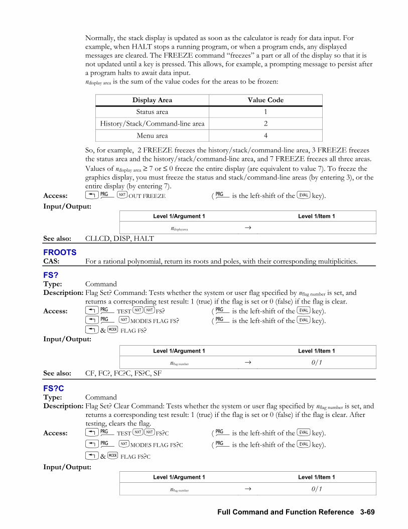
Full Command and Function Reference 3-69
Normally, the stack display is updated as soon as the calculator is ready for data input. For example, when HALT stops a running program, or when a program ends, any displayed messages are cleared. The FREEZE command freezes a part or all of the display so that it is not updated until a key is pressed. This allows, for example, a prompting message to persist after a program halts to await data input.
ndisplay area is the sum of the value codes for the areas to be frozen:
Display Area Value Code Status area 1
History/Stack/Command-line area 2 Menu area 4
So, for example, 2 FREEZE freezes the history/stack/command-line area, 3 FREEZE freezes the status area and the history/stack/command-line area, and 7 FREEZE freezes all three areas.
Values of ndisplay area ≥ 7 or ≤ 0 freeze the entire display (are equivalent to value 7). To freeze the graphics display, you must freeze the status and stack/command-line areas (by entering 3), or the entire display (by entering 7).
Access: !°LOUT FREEZE ( °is the left-shift of the Nkey). Input/Output:
Level 1/Argument 1 Level 1/Item 1
ndisplayarea → See also: CLLCD, DISP, HALT
FROOTS CAS: For a rational polynomial, return its roots and poles, with their corresponding multiplicities.
FS? Type: Command Description: Flag Set? Command: Tests whether the system or user flag specified by nflag number is set, and
returns a corresponding test result: 1 (true) if the flag is set or 0 (false) if the flag is clear. Access: !°TEST LLFS? ( °is the left-shift of the Nkey). !° LMODES FLAG FS? ( °is the left-shift of the Nkey). !& H FLAG FS? Input/Output:
Level 1/Argument 1 Level 1/Item 1
nflag number → 0/1 See also: CF, FC?, FC?C, FS?C, SF
FS?C Type: Command Description: Flag Set? Clear Command: Tests whether the system or user flag specified by nflag number is set, and
returns a corresponding test result: 1 (true) if the flag is set or 0 (false) if the flag is clear. After testing, clears the flag.
Access: !°TEST LLFS?C ( °is the left-shift of the Nkey). !° LMODES FLAG FS?C ( °is the left-shift of the Nkey). !& H FLAG FS?C Input/Output:
Level 1/Argument 1 Level 1/Item 1
nflag number → 0/1
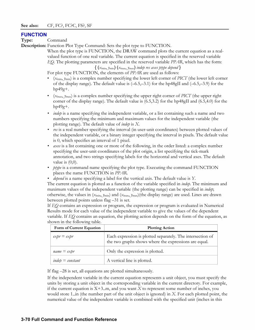
3-70 Full Command and Function Reference
See also: CF, FC?, FC?C, FS?, SF
FUNCTION Type: Command Description: Function Plot Type Command: Sets the plot type to FUNCTION. When the plot type is FUNCTION, the DRAW command plots the current equation as a real-
valued function of one real variable. The current equation is specified in the reserved variable EQ. The plotting parameters are specified in the reserved variable PPAR, which has the form:
(xmin, ymin) (xmax, ymax) indep res axes ptype depend For plot type FUNCTION, the elements of PPAR are used as follows:
(xmin, ymin) is a complex number specifying the lower left corner of PICT (the lower left corner of the display range). The default value is (6.5,3.1) for the hp48gII and (6.5,3.9) for the hp49g+.
(xmax, ymax) is a complex number specifying the upper right corner of PICT (the upper right corner of the display range). The default value is (6.5,3.2) for the hp48gII and (6.5,4.0) for the hp49g+.
indep is a name specifying the independent variable, or a list containing such a name and two numbers specifying the minimum and maximum values for the independent variable (the plotting range). The default value of indep is X.
res is a real number specifying the interval (in user-unit coordinates) between plotted values of the independent variable, or a binary integer specifying the interval in pixels. The default value is 0, which specifies an interval of 1 pixel.
axes is a list containing one or more of the following, in the order listed: a complex number specifying the user-unit coordinates of the plot origin, a list specifying the tick-mark annotation, and two strings specifying labels for the horizontal and vertical axes. The default value is (0,0).
ptype is a command name specifying the plot type. Executing the command FUNCTION places the name FUNCTION in PPAR.
depend is a name specifying a label for the vertical axis. The default value is Y. The current equation is plotted as a function of the variable specified in indep. The minimum and
maximum values of the independent variable (the plotting range) can be specified in indep; otherwise, the values in (xmin, ymin) and (xmax, ymax)(the display range) are used. Lines are drawn between plotted points unless flag 31 is set.
If EQ contains an expression or program, the expression or program is evaluated in Numerical Results mode for each value of the independent variable to give the values of the dependent variable. If EQ contains an equation, the plotting action depends on the form of the equation, as shown in the following table.
Form of Current Equation Plotting Action
expr = expr Each expression is plotted separately. The intersection of the two graphs shows where the expressions are equal.
name = expr Only the expression is plotted.
indep = constant A vertical line is plotted. If flag 28 is set, all equations are plotted simultaneously. If the independent variable in the current equation represents a unit object, you must specify the
units by storing a unit object in the corresponding variable in the current directory. For example, if the current equation is X+3_m, and you want X to represent some number of inches, you would store 1_in (the number part of the unit object is ignored) in X. For each plotted point, the numerical value of the independent variable is combined with the specified unit (inches in this
Full Command and Function Reference 3-71
example) before the current equation is evaluated. If the result is a unit object, only the number part is plotted.
Access: µFUNCTION Flags: Simultaneous Plotting (-28), Curve Filling (-31) Input/Output: None See also: BAR, CONIC, DIFFEQ, FAST3D, GRIDMAP, HISTOGRAM, PARAMETRIC,
PARSURFACE, PCONTOUR, POLAR, SCATTER, SLOPEFIELD, TRUTH, WIREFRAME, YSLICE
FXND CAS: Split a fractional object into its numerator and denominator.
GAMMA Type: Function Description: Evaluate the Γ function at the given point. For a positive integer x, Γ(x) is equal to (x +1)!
GAMMA differs from the FACT and ! functions because it allows complex arguments. The Γ function is defined by
Γ x( ) e t tx 1⋅ td0
+∞∫=
. Access: !´LSPECIAL Input: A real or complex number, x. Output: Γ(x). If the input x is an integer greater than 100, returns the symbolic expression GAMMA(x). Flags: If the Underflow Exception (20) or Overflow Exception (21) flags are set then underflow or
overflow conditions give errors, otherwise they give zero or the maximum real number the calculator can express. Complex mode must be set (flag 103 set) if x is complex.
See also: FACT, PSI, Psi, !
GAUSS CAS: Return the diagonal representation of a quadratic form.
GBASIS CAS: Return a set of polynomials that are a Grbner basis G of the ideal I of an input set of
polynomials.
GCD CAS: Return the greatest common divisor of two objects.
GCDMOD CAS: Find the greatest common divisor of two polynomials modulo the current modulus.
GET Type: Command Description: Get Element Command: Returns from the argument 1/level 2 array or list (or named array or
list) the real or complex number zget or object objget whose position is specified in argument 2/level 1. For matrices, nposition is incremented in row order.
Access: !°LIST ELEMENTS GET ( °is the left-shift of the Nkey).
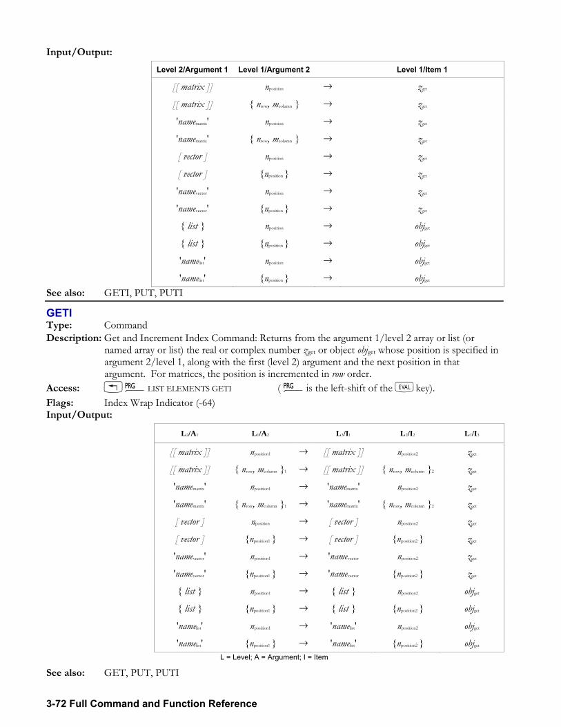
3-72 Full Command and Function Reference
Input/Output: Level 2/Argument 1 Level 1/Argument 2 Level 1/Item 1
[[ matrix ]] nposition → zget
[[ matrix ]] nrow, mcolumn → zget
'namematrix' nposition → zget
'namematrix' nrow, mcolumn → zget
[ vector ] nposition → zget
[ vector ] nposition → zget
'namevector' nposition → zget
'namevector' nposition → zget
list nposition → objget
list nposition → objget
'namelist' nposition → objget
'namelist' nposition → objget See also: GETI, PUT, PUTI
GETI Type: Command Description: Get and Increment Index Command: Returns from the argument 1/level 2 array or list (or
named array or list) the real or complex number zget or object objget whose position is specified in argument 2/level 1, along with the first (level 2) argument and the next position in that argument. For matrices, the position is incremented in row order.
Access: !°LIST ELEMENTS GETI ( °is the left-shift of the Nkey). Flags: Index Wrap Indicator (-64) Input/Output:
L2/A1 L1/A2 L3/I1 L2/I2 L1/I3
[[ matrix ]] nposition1 → [[ matrix ]] nposition2 zget
[[ matrix ]] nrow, mcolumn 1 → [[ matrix ]] nrow, mcolumn 2 zget
'namematrix' nposition1 → 'namematrix' nposition2 zget
'namematrix' nrow, mcolumn 1 → 'namematrix' nrow, mcolumn 2 zget
[ vector ] nposition → [ vector ] nposition2 zget
[ vector ] nposition1 → [ vector ] nposition2 zget
'namevector' nposition1 → 'namevector nposition2 zget
'namevector' nposition1 → 'namevector nposition2 zget
list nposition1 → list nposition2 objget
list nposition1 → list nposition2 objget
'namelist' nposition1 → 'namelist' nposition2 objget
'namelist' nposition1 → 'namelist' nposition2 objget L = Level; A = Argument; I = Item
See also: GET, PUT, PUTI
Full Command and Function Reference 3-73
GOR Type: Command Description: Graphics OR Command: Superimposes grob1 onto grobtarget or PICT, with the upper left corner
pixel of grob1 positioned at the specified coordinate in grobtarget or PICT. GOR uses a logical OR to determine the state (on or off) of each pixel in the overlapping
portion of the argument graphics object. If the first argument (stack level 3) is any graphics object other than PICT, then grobresult is
returned to the stack. If the first argument (level 3) is PICT, no result is returned to the stack. Any portion of grob1 that extends past grobtarget or PICT is truncated. Access: !°L GROB GOR ( °is the left-shift of the Nkey). Input/Output:
Level 3/Argument 1 Level 2/Argument 2 Level 1/Argument 3 Level 1/Item 1
grobtarget #n #m grob1 → grobresult
grobtarget (x, y) grob1 → grobresult
PICT #n #m grob1 →
PICT (x, y) grob1 →
See also: GXOR, REPL, SUB
GRAD Type: Command Description: Grads Mode Command: Sets Grads angle mode. GRAD clears flag 17 and sets flag 18, and displays the GRD annunciator. In Grads angle mode, real-number arguments that represent angles are interpreted as grads, and
real-number results that represent angles are expressed in grads. Access: !&HANGLE GRAD µ GRAD Input/Output: None See also: DEG, RAD
GRAMSCHMIDT CAS: Find an orthonormal base of a vector space with respect to a given scalar product.
GREDUCE CAS: Reduce a polynomial with respect to a Grbner basis.
GRIDMAP Type: Command Description: GRIDMAP Plot Type Command: Sets the plot type to GRIDMAP. When plot type is set GRIDMAP, the DRAW command plots a mapping grid representation of
a 2-vector-valued function of two variables. GRIDMAP requires values in the reserved variables EQ, VPAR, and PPAR.
VPAR has the following form: xleft, xright, ynear, yfar, zlow, zhigh, xmin, xmax, ymin, ymax, xeye, yeye, zeye, xstep, ystep
For plot type GRIDMAP, the elements of VPAR are used as follows: xleft and xright are real numbers that specify the width of the view space. ynear and yfar are real numbers that specify the depth of the view space. zlow and zhigh are real numbers that specify the height of the view space.
3-74 Full Command and Function Reference
xmin and xmax are real numbers that specify the input region's width. The default value is (1,1).
ymin and ymax are real numbers that specify the input region's depth. The default value is (1,1). xeye, yeye, and zeye are real numbers that specify the point in space from which you view the
graph. xstep and ystep are real numbers that set the number of x-coordinates versus the number of y-
coordinates plotted. These can be used instead of (or in combination with) RES. The plotting parameters are specified in the reserved variable PPAR, which has the following form: (xmin, ymin), (xmax, ymax), indep, res, axes, ptype, depend For plot type GRIDMAP, the elements of PPAR are used as follows:
(xmin, ymin) is not used. (xmax, ymax) is not used. indep is a name specifying the independent variable. The default value of indep is X. res is a real number specifying the interval (in user-unit coordinates) between plotted values of
the independent variable, or a binary integer specifying the interval in pixels. The default value is 0, which specifies an interval of 1 pixel.
axes is not used. ptype is a command name specifying the plot type. Executing the command GRIDMAP places
the command name GRIDMAP in PPAR. depend is a name specifying the dependent variable. The default value is Y.
Access: µ GRIDMAP Input/Output: None See also: BAR, CONIC, DIFFEQ, FUNCTION, HISTOGRAM, PARAMETRIC, PARSURFACE,
PCONTOUR, POLAR, SCATTER, SLOPEFIELD, TRUTH, WIREFRAME, YSLICE
→GROB Type: Command Description: Stack to Graphics Object Command: Creates a graphics object from a specified object, where the
argument nchar size specifies the character size of the object. nchar size can be 0, 1 (small), 2 (medium), or 3 (large). nchar size = 0 is the same as nchar size = 3, except
for unit objects and algebraic objects, where 0 specifies the Equation Writer application picture. Access: µ→GROB !°LGROB →GROB ( °is the left-shift of the Nkey). Input/Output:
Level 2/Argument 1 Level 1/Argument 2 Level 1/Item 1
obj ncharsize → grob See also: →LCD, LCD→
GROB Type: Command Description: Enters GROB on the command line to help with the manual entry of a graphic object. Access: µGROB
GROBADD Type: Command Description: Combines two graphic objects by appending the second argument onto the bottom of the first. Access: PGRAPH GROBADD !ÖGRAPH GROBADD ( Ö is the left-shift of the 4key).
Full Command and Function Reference 3-75
Input/Output:
Level 2/Argument 1 Level 1/Argument 2 Level 1/Item 1
GROB1 GROB2 → GROB3
GXOR Type: Command Description: Graphics Exclusive OR Command: Superimposes grob1 onto grobtarget or PICT, with the upper left
corner pixel of grob1 positioned at the specified coordinate in grobtarget or PICT. GXOR is used for creating cursors, for example, to make the cursor image appear dark on a light
background and light on a dark background. Executing GXOR again with the same image restores the original picture.
GXOR uses a logical exclusive OR to determine the state of the pixels (on or off) in the overlapping portion of the argument graphics objects.
Any portion of grob1 that extends past grobtarget or PICT is truncated. If the first (level 3) argument (the target graphics object) is any graphics object other than PICT,
then grobresult is returned to the stack. If the first (level 3) argument is PICT, no result is returned to the stack.
Access: !°L GROB GXOR ( °is the left-shift of the Nkey). Input/Output:
Level 3/Argument 1 Level 2/Argument 2 Level 1/Argument 3 Level 1/Item 1
grobtarget #n, #m grob1 → grobresult
grobtarget (x, y) grob1 → grobresult
PICT #n, #m grob1 →
PICT (x, y) grob1 →
See also: GOR, REPL, SUB
HADAMARD CAS: Perform an element by element multiplication of two matrices (Hadamard product).
HALFTAN CAS: Transform an expression by replacing sin(x), cos(x) and tan(x) subexpressions with tan(x/2).
HALT Type: Command Description: Halt Program Command: Halts program execution. Program execution is halted at the location of the HALT command in the program. The HLT
annunciator is turned on. Program execution is resumed by executing CONT (that is, by pressing !æ). Executing KILL cancels all halted programs.
Access: !°LL RUN & DEBUG HALT ( °is the left-shift of the Nkey). Input/Output: None See also: CONT, KILL
HEAD Type: Command Description: First Listed Element Command: Returns the first element of a list or string.
3-76 Full Command and Function Reference
Access: !°LCHARS LHEAD ( °is the left-shift of the Nkey). !°LIST ELEMEN LHEAD ( °is the left-shift of the Nkey). ± LHEAD (± is the right-shift of the Nkey). Input/Output:
Level 1/Argument 1 Level 1/Item 1
obj1, ... ,objn → obj1
string → element1 See also: TAIL
HEADER→ Type: Command Description: Header size: Returns the current size of the header in lines. Access: µHEADER→ Input/Output:
Level 1/Argument 1 Level 1/Item 1
→ Header size See also: →HEADER
→HEADER Type: Command Description: Header size: Sets the current size of the header in lines: to 0, 1, or 2 lines. Access: µ→HEADER Input/Output:
Level 1/Argument 1 Level 1/Item 1
Header size → See also: HEADER→
HELP CAS: Display CAS operations and help information for them.
HERMITE CAS: Return the nth Hermite polynomial.
HESS CAS: Return the Hessian matrix and the gradient of an expression with respect to specified variables.
HEX Type: Command Description: Hexadecimal Mode Command: Selects hexadecimal base for binary integer operations. (The
default base is decimal.) Binary integers require the prefix #. Binary integers entered and returned in hexadecimal base
automatically show the suffix h. If the current base is not hexadecimal, then you can enter a hexadecimal number by ending it with h. It will be displayed in the current base when it is entered.
The current base does not affect the internal representation of binary integers as unsigned binary numbers.
Full Command and Function Reference 3-77
Access: !´BASE HEX ( ´ is the left-shift of the Pkey). !Ú BASE HEX ( Ú is the left-shift of the 6key). Flags: Binary Integer Wordsize (5 through 10), Binary Integer Base (11, 12) Input/Output: None See also: BIN, DEC, OCT, RCWS, STWS
HILBERT CAS: Return a square Hilbert matrix of specified order.
HISTOGRAM Type: Command Description: Histogram Plot Type Command: Sets the plot type to HISTOGRAM. When the plot type is HISTOGRAM, the DRAW command creates a histogram using data from
one column of the current statistics matrix (reserved variable ΣDAT). The column is specified by the first parameter in the reserved variable ΣPAR (using the XCOL command). The plotting parameters are specified in the reserved variable PPAR, which has the form:
(xmin, ymin) (xmax, ymax) indep res axes ptype depend For plot type HISTOGRAM, the elements of PPAR are used as follows:
(xmin, ymin) is a complex number specifying the lower left corner of PICT (the lower left corner of the display range). The default value is (6.5,3.1) for the hp48gII and (6.5,3.9) for the hp49g+.
(xmax, ymax) is a complex number specifying the upper right corner of PICT (the upper right corner of the display range). The default value is (6.5,3.2) for the hp48gII and (6.5,4.0) for the hp49g+.
indep is either a name specifying a label for the horizontal axis, or a list containing such a name and two numbers that specify the minimum and maximum values of the data to be plotted. The default value of indep is X.
res is a real number specifying the bin size, in user-unit coordinates, or a binary integer specifying the bin size in pixels. The default value is 0, which specifies the bin size to be 1/13 of the difference between the specified minimum and maximum values of the data.
axes is a list containing one or more of the following, in the order listed: a complex number specifying the user-unit coordinates of the plot origin, a list specifying the tick-mark annotation, and two strings specifying labels for the horizontal and vertical axes. The default value is (0,0).
ptype is a command name specifying the plot type. Executing the command HISTOGRAM places the command name HISTOGRAM in PPAR.
depend is a name specifying a label for the vertical axis. The default value is Y. The frequency of the data is plotted as bars, where each bar represents a collection of data
points. The base of each bar spans the values of the data points, and the height indicates the number of data points. The width of each bar is specified by res. The overall maximum and minimum values for the data can be specified by indep; otherwise, the values in (xmin, ymin) and (xmax, ymax) are used.
Access: µ HISTOGRAM Input/Output: None See also: BAR, CONIC, DIFFEQ, FUNCTION, GRIDMAP, PARAMETRIC, PARSURFACE,
PCONTOUR, POLAR, SCATTER, SLOPEFIELD, TRUTH, WIREFRAME, YSLICE
HISTPLOT Type: Command
3-78 Full Command and Function Reference
Description: Draw Histogram Plot Command: Plots a frequency histogram of the specified column in the current statistics matrix (reserved variable ΣDAT).
The data column to be plotted is specified by XCOL and is stored as the first parameter in the reserved variable ΣPAR. If no data column is specified, column 1 is selected by default. The y-axis is autoscaled and the plot type is set to HISTOGRAM.
HISTPLOT plots relative frequencies, using 13 bins as the default number of partitions. The RES command lets you specify a different number of bins by specifying the bin width. To plot a frequency histogram with numerical frequencies, store the frequencies in ΣDAT and execute BINS and then BARPLOT.
When HISTPLOT is executed from a program, the graphics display, which shows the resultant plot, does not persist unless PICTURE, PVIEW (with an empty list argument), or FREEZE is subsequently executed.
Access: µ HISTPLOT Input/Output: None See also: BARPLOT, BINS, FREEZE, PICTURE, PVIEW, RES, SCATRPLOT, XCOL
HMS Type: Command Description: Hours-Minutes-Seconds Minus Command: Returns the difference of two real numbers, where
the arguments and the result are interpreted in hours-minutes-seconds format. The format for HMS (a time or an angle) is H.MMSSs, where:
H is zero or more digits representing the integer part of the number (hours or degrees). MM are two digits representing the number of minutes. SS are two digits representing the number of seconds. s is zero or more digits (as many as allowed by the current display mode) representing the
decimal fractional part of seconds. Access: ÓTools LHMS ( Ó is the right-shift of the 9 key). & 9LHMS Input/Output:
Level 2/Argument 1 Level 1/Argument 2 Level 1/Item 1
HMS1 HMS2 → HMS1 HMS2 See also: HMS→, →HMS, HMS+
HMS+ Type: Command Description: Hours-Minutes-Seconds Plus Command: Returns the sum of two real numbers, where the
arguments and the result are interpreted in hours-minutes-seconds format. The format for HMS (a time or an angle) is H.MMSSs, where:
H is zero or more digits representing the integer part of the number (hours or degrees). MM are two digits representing the number of minutes. SS are two digits representing the number of seconds. s is zero or more digits (as many as allowed by the current display mode) representing the
decimal fractional part of seconds. Access: ÓTools LHMS+ ( Ó is the right-shift of the 9 key). & 9LHMS+ Input/Output:
Level 2/Argument 1 Level 1/Argument 2 Level 1/Item 1
HMS1 HMS2 → HMS1 + HMS2
Full Command and Function Reference 3-79
See also: HMS→, →HMS, HMS
HMS→ Type: Command Description: Hours-Minutes-Seconds to Decimal Command: Converts a real number in hours-minutes-
seconds format to its decimal form (hours or degrees with a decimal fraction). The format for HMS (a time or an angle) is H.MMSSs, where:
H is zero or more digits representing the integer part of the number (hours or degrees). MM are two digits representing the number of minutes. SS are two digits representing the number of seconds. s is zero or more digits (as many as allowed by the current display mode) representing the
decimal fractional part of seconds. Access: ÓTools L HMS→ ( Ó is the right-shift of the 9 key). &9L HMS→ Input/Output:
Level 1/Argument 1 Level 1/Item 1
HMS → x See also: →HMS, HMS+, HMS
→HMS Type: Command Description: Decimal to Hours-Minutes-Seconds Command: Converts a real number representing hours or
degrees with a decimal fraction to hours-minutes-seconds format. The format for HMS (a time or an angle) is H.MMSSs, where:
H is zero or more digits representing the integer part of the number. MM are two digits representing the number of minutes. SS are two digits representing the number of seconds. s is zero or more digits (as many as allowed by the current display mode) representing the
decimal fractional part of seconds. Access: ÓTools L→HMS ( Ó is the right-shift of the 9 key). &9L→HMS Input/Output:
Level 1/Argument 1 Level 1/Item 1
x → HMS See also: HMS→, HMS+, HMS
HOME Type: Command Description: HOME Directory Command: Makes the HOME directory the current directory. Access: µ HOME !& J Input/Output: None See also: CRDIR, PATH, PGDIR, UPDIR
HORNER CAS: Execute a Horner scheme;. for polynomial P, and number r, return P/(xr), r and P(r).
3-80 Full Command and Function Reference
i Type: Function Description: i Function: Returns the symbolic constant i or its numerical representation, (0, 1). Access: !¥ (¥is the left-shift of the Ikey). Flags: Symbolic Constants (2), Numerical Results (3) Input/Output:
Level 1/Argument 1 Level 1/Item 1
→ 'i' → (0,1)
See also: e, MAXR, MINR, π
IABCUV CAS: Return a solution in integers u and v of au + bv = c, where a, b, and c are integers.
IBASIS CAS: Determine the basis of the intersection between two vector spaces.
IBERNOULLI CAS: Return the nth Bernoulli number for a given integer n.
IBP CAS: Integration by parts of a product of two functions, given the antiderivative of one function.
ICHINREM CAS: Solve a system of two congruences in integers using the Chinese Remainder theorem.
IDN Type: Command Description: Identity Matrix Command: Returns an identity matrix; that is, a square matrix with its diagonal
elements equal to 1 and its off-diagonal elements equal to 0. The result is either a new square matrix, or an existing square matrix with its elements replaced
by the elements of the identity matrix, according to the argument. Creating a new matrix: If the argument is a real number n, a new real identity matrix is
returned, with its number of rows and number of columns equal to n. Replacing the elements of an existing matrix: If the argument is a square matrix, an identity
matrix of the same dimensions is returned. If the original matrix is complex, the resulting identity matrix will also be complex, with diagonal values (1,0).
If the argument is a name, the name must identify a variable containing a square matrix. In this case, the elements of the matrix are replaced by those of the identity matrix (complex if the original matrix is complex).
Access: !Ø CREATE IDN ( Ø is the left-shift of the 5key). !´MATRIX MAKE IDN ( ´ is the left-shift of the Pkey). Input/Output:
Level 1/Argument 1 Level 1/Item 1
n → [[ R-matrixidentity ]] [[ matrix ]] → [[ matrixidentity ]]
'name' → [[ matrixidentity ]]
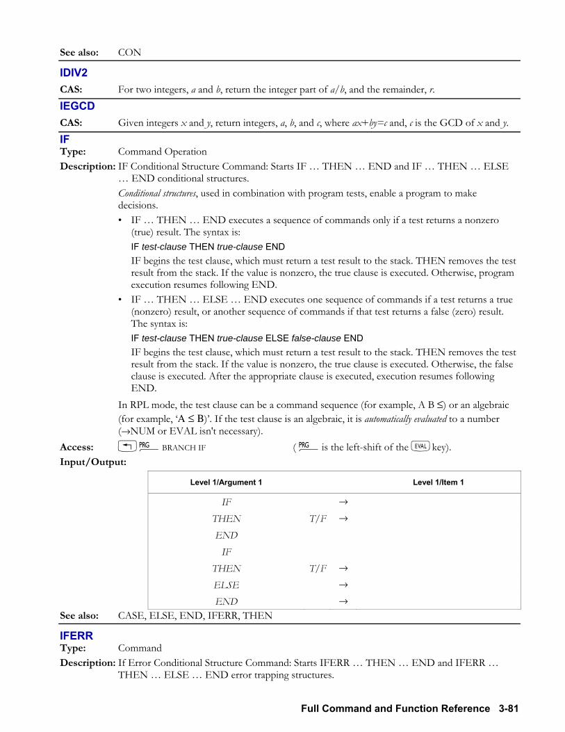
Full Command and Function Reference 3-81
See also: CON
IDIV2 CAS: For two integers, a and b, return the integer part of a/b, and the remainder, r.
IEGCD CAS: Given integers x and y, return integers, a, b, and c, where ax+by=c and, c is the GCD of x and y.
IF Type: Command Operation Description: IF Conditional Structure Command: Starts IF THEN END and IF THEN ELSE
END conditional structures. Conditional structures, used in combination with program tests, enable a program to make
decisions. IF THEN END executes a sequence of commands only if a test returns a nonzero
(true) result. The syntax is: IF test-clause THEN true-clause END IF begins the test clause, which must return a test result to the stack. THEN removes the test result from the stack. If the value is nonzero, the true clause is executed. Otherwise, program execution resumes following END.
IF THEN ELSE END executes one sequence of commands if a test returns a true (nonzero) result, or another sequence of commands if that test returns a false (zero) result. The syntax is: IF test-clause THEN true-clause ELSE false-clause END IF begins the test clause, which must return a test result to the stack. THEN removes the test result from the stack. If the value is nonzero, the true clause is executed. Otherwise, the false clause is executed. After the appropriate clause is executed, execution resumes following END.
In RPL mode, the test clause can be a command sequence (for example, A B ≤) or an algebraic (for example, Α ≤ Β). If the test clause is an algebraic, it is automatically evaluated to a number (→NUM or EVAL isn't necessary).
Access: !°BRANCH IF ( °is the left-shift of the Nkey). Input/Output:
Level 1/Argument 1 Level 1/Item 1
IF → THEN T/F → END
IF THEN T/F → ELSE → END →
See also: CASE, ELSE, END, IFERR, THEN
IFERR Type: Command Description: If Error Conditional Structure Command: Starts IFERR THEN END and IFERR
THEN ELSE END error trapping structures.
3-82 Full Command and Function Reference
Error trapping structures enable program execution to continue after a trapped error occurs. IFERR THEN END executes a sequence of commands if an error occurs. The syntax
of IFERR THEN END is: IFERR trap-clause THEN error-clause END If an error occurs during execution of the trap clause: 1 The error is ignored. 2 The remainder of the trap clause is discarded. 3 The key buffer is cleared. 4 If any or all of the display is frozen (by FREEZE), that state is cancelled. 5 If Last Arguments is enabled, the arguments to the command that caused the error are
returned to the stack. 6 Program execution jumps to the error clause. The commands in the error clause are executed only if an error is generated during execution of the trap clause.
IFERR THEN ELSE END executes one sequence of commands if an error occurs or another sequence of commands if an error does not occur. The syntax of IFERR THEN ELSE END is: IFERR trap-clause THEN error-clause ELSE normal-clause END If an error occurs during execution of the trap clause, the same six events listed above occur. If no error occurs, execution jumps to the normal clause at the completion of the trap clause.
Access: !°LLERROR [IFERR] IFERR ( °is the left-shift of the Nkey). Flags: Last Arguments (-55) Input/Output: None See also: CASE, ELSE, END, IF, THEN
IFFT Type: Command Description: Inverse Discrete Fourier Transform Command: Computes the one- or two-dimensional inverse
discrete Fourier transform of an array. If the argument is an N-vector or an N × 1 or 1 × N matrix, IFFT computes the one-
dimensional inverse transform. If the argument is an M × N matrix, IFFT computes the two-dimensional inverse transform. M and N must be integral powers of 2.
The one-dimensional inverse discrete Fourier transform of an N-vector Y is the N-vector X where:
Xn1N----
Yke2π ikn
N---------------
k 0=
N 1
∑= i, 1=
for n = 0, 1, , N 1. The two-dimensional inverse discrete Fourier transform of an M × N matrix Y is the M × N
matrix X where:
Xmn1
MN--------- Ykle2π ikm
M----------------e
2π i lnN------------------
l 0=
N 1∑
k 0=
M 1∑= i, 1=
for m = 0, 1, , M 1 and n = 0, 1, , N 1. The discrete Fourier transform and its inverse are defined for any positive sequence length.
However, the calculation can be performed very rapidly when the sequence length is a power of
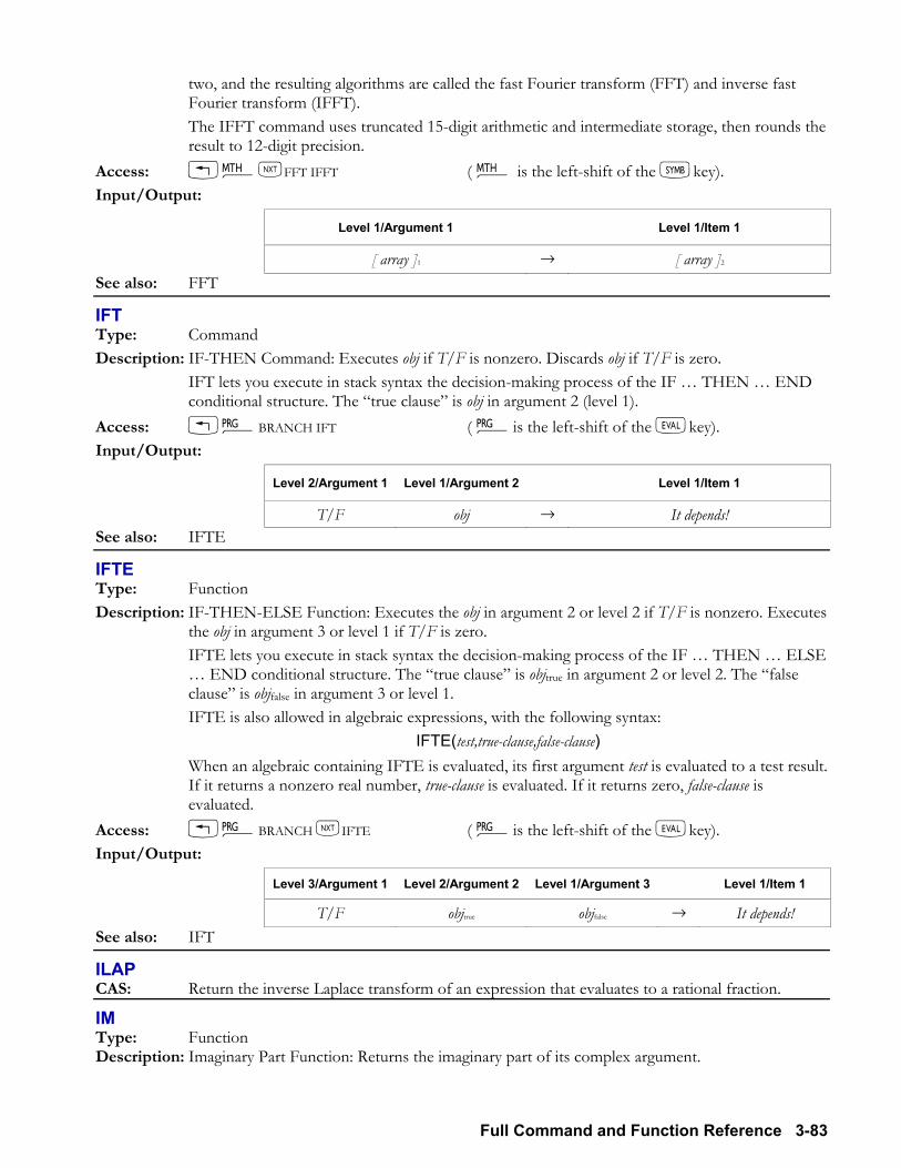
Full Command and Function Reference 3-83
two, and the resulting algorithms are called the fast Fourier transform (FFT) and inverse fast Fourier transform (IFFT).
The IFFT command uses truncated 15-digit arithmetic and intermediate storage, then rounds the result to 12-digit precision.
Access: !´LFFT IFFT ( ´ is the left-shift of the Pkey). Input/Output:
Level 1/Argument 1 Level 1/Item 1
[ array ]1 → [ array ]2 See also: FFT
IFT Type: Command Description: IF-THEN Command: Executes obj if T/F is nonzero. Discards obj if T/F is zero. IFT lets you execute in stack syntax the decision-making process of the IF THEN END
conditional structure. The true clause is obj in argument 2 (level 1). Access: !°BRANCH IFT ( °is the left-shift of the Nkey). Input/Output:
Level 2/Argument 1 Level 1/Argument 2 Level 1/Item 1
T/F obj → It depends! See also: IFTE
IFTE Type: Function Description: IF-THEN-ELSE Function: Executes the obj in argument 2 or level 2 if T/F is nonzero. Executes
the obj in argument 3 or level 1 if T/F is zero. IFTE lets you execute in stack syntax the decision-making process of the IF THEN ELSE
END conditional structure. The true clause is objtrue in argument 2 or level 2. The false clause is objfalse in argument 3 or level 1.
IFTE is also allowed in algebraic expressions, with the following syntax: IFTE(test,true-clause,false-clause)
When an algebraic containing IFTE is evaluated, its first argument test is evaluated to a test result. If it returns a nonzero real number, true-clause is evaluated. If it returns zero, false-clause is evaluated.
Access: !°BRANCH LIFTE ( °is the left-shift of the Nkey). Input/Output:
Level 3/Argument 1 Level 2/Argument 2 Level 1/Argument 3 Level 1/Item 1
T/F objtrue objfalse → It depends! See also: IFT
ILAP CAS: Return the inverse Laplace transform of an expression that evaluates to a rational fraction.
IM Type: Function Description: Imaginary Part Function: Returns the imaginary part of its complex argument.
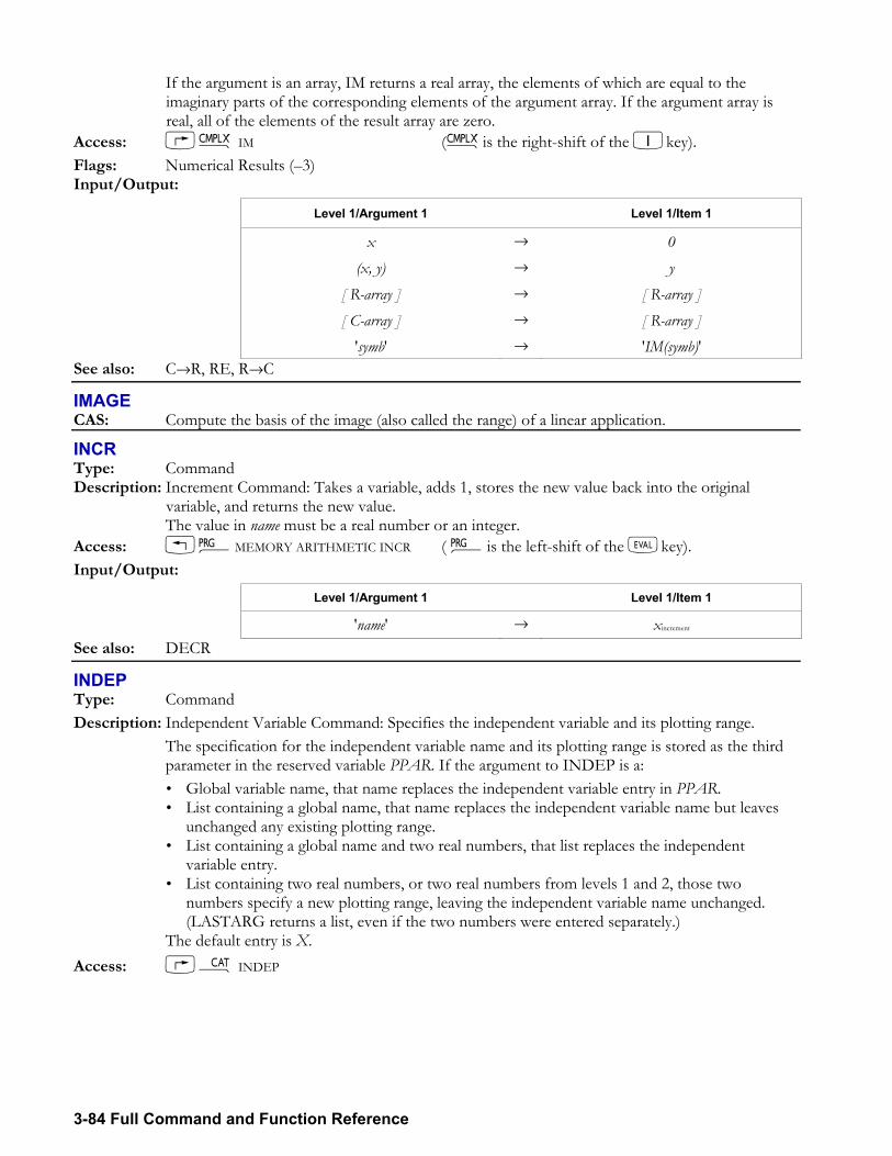
3-84 Full Command and Function Reference
If the argument is an array, IM returns a real array, the elements of which are equal to the imaginary parts of the corresponding elements of the argument array. If the argument array is real, all of the elements of the result array are zero.
Access: ß IM (ßis the right-shift of the 1key). Flags: Numerical Results (3) Input/Output:
Level 1/Argument 1 Level 1/Item 1
x → 0 (x, y) → y
[ R-array ] → [ R-array ] [ C-array ] → [ R-array ]
'symb' → 'IM(symb)' See also: C→R, RE, R→C
IMAGE CAS: Compute the basis of the image (also called the range) of a linear application.
INCR Type: Command Description: Increment Command: Takes a variable, adds 1, stores the new value back into the original
variable, and returns the new value. The value in name must be a real number or an integer. Access: !°MEMORY ARITHMETIC INCR ( °is the left-shift of the Nkey). Input/Output:
Level 1/Argument 1 Level 1/Item 1
'name' → xincrement See also: DECR
INDEP Type: Command Description: Independent Variable Command: Specifies the independent variable and its plotting range. The specification for the independent variable name and its plotting range is stored as the third
parameter in the reserved variable PPAR. If the argument to INDEP is a: Global variable name, that name replaces the independent variable entry in PPAR. List containing a global name, that name replaces the independent variable name but leaves
unchanged any existing plotting range. List containing a global name and two real numbers, that list replaces the independent
variable entry. List containing two real numbers, or two real numbers from levels 1 and 2, those two
numbers specify a new plotting range, leaving the independent variable name unchanged. (LASTARG returns a list, even if the two numbers were entered separately.)
The default entry is X. Access: µ INDEP
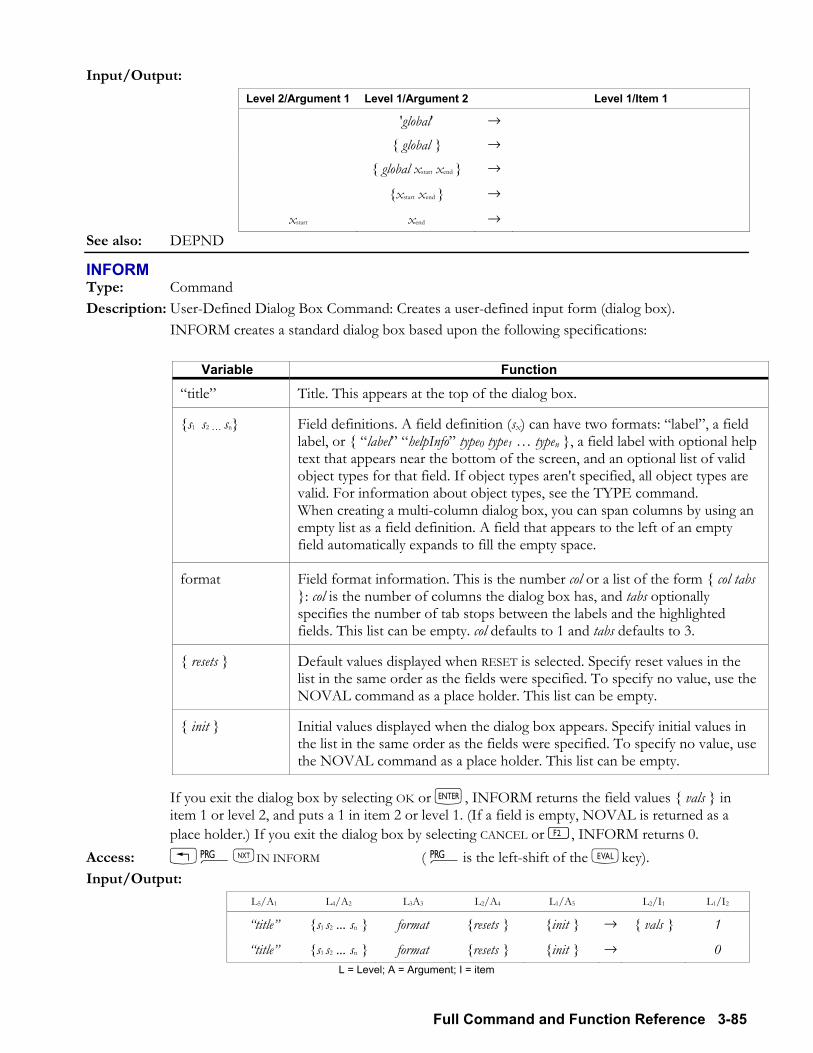
Full Command and Function Reference 3-85
Input/Output: Level 2/Argument 1 Level 1/Argument 2 Level 1/Item 1
'global' → global → global xstart xend →
xstart xend →
xstart xend → See also: DEPND
INFORM Type: Command Description: User-Defined Dialog Box Command: Creates a user-defined input form (dialog box). INFORM creates a standard dialog box based upon the following specifications:
Variable Function
title Title. This appears at the top of the dialog box.
s1 s2 sn Field definitions. A field definition (sx) can have two formats: label, a field label, or label helpInfo type0 type1 typen , a field label with optional help text that appears near the bottom of the screen, and an optional list of valid object types for that field. If object types aren't specified, all object types are valid. For information about object types, see the TYPE command. When creating a multi-column dialog box, you can span columns by using an empty list as a field definition. A field that appears to the left of an empty field automatically expands to fill the empty space.
format Field format information. This is the number col or a list of the form col tabs : col is the number of columns the dialog box has, and tabs optionally specifies the number of tab stops between the labels and the highlighted fields. This list can be empty. col defaults to 1 and tabs defaults to 3.
resets Default values displayed when RESET is selected. Specify reset values in the list in the same order as the fields were specified. To specify no value, use the NOVAL command as a place holder. This list can be empty.
init Initial values displayed when the dialog box appears. Specify initial values in the list in the same order as the fields were specified. To specify no value, use the NOVAL command as a place holder. This list can be empty.
If you exit the dialog box by selecting OK or `, INFORM returns the field values vals in item 1 or level 2, and puts a 1 in item 2 or level 1. (If a field is empty, NOVAL is returned as a place holder.) If you exit the dialog box by selecting CANCEL or B, INFORM returns 0.
Access: !°LIN INFORM ( °is the left-shift of the Nkey). Input/Output:
L5/A1 L4/A2 L3A3 L2/A4 L1/A5 L2/I1 L1/I2
title s1 s2 ... sn format resets init → vals 1
title s1 s2 ... sn format resets init → 0 L = Level; A = Argument; I = item
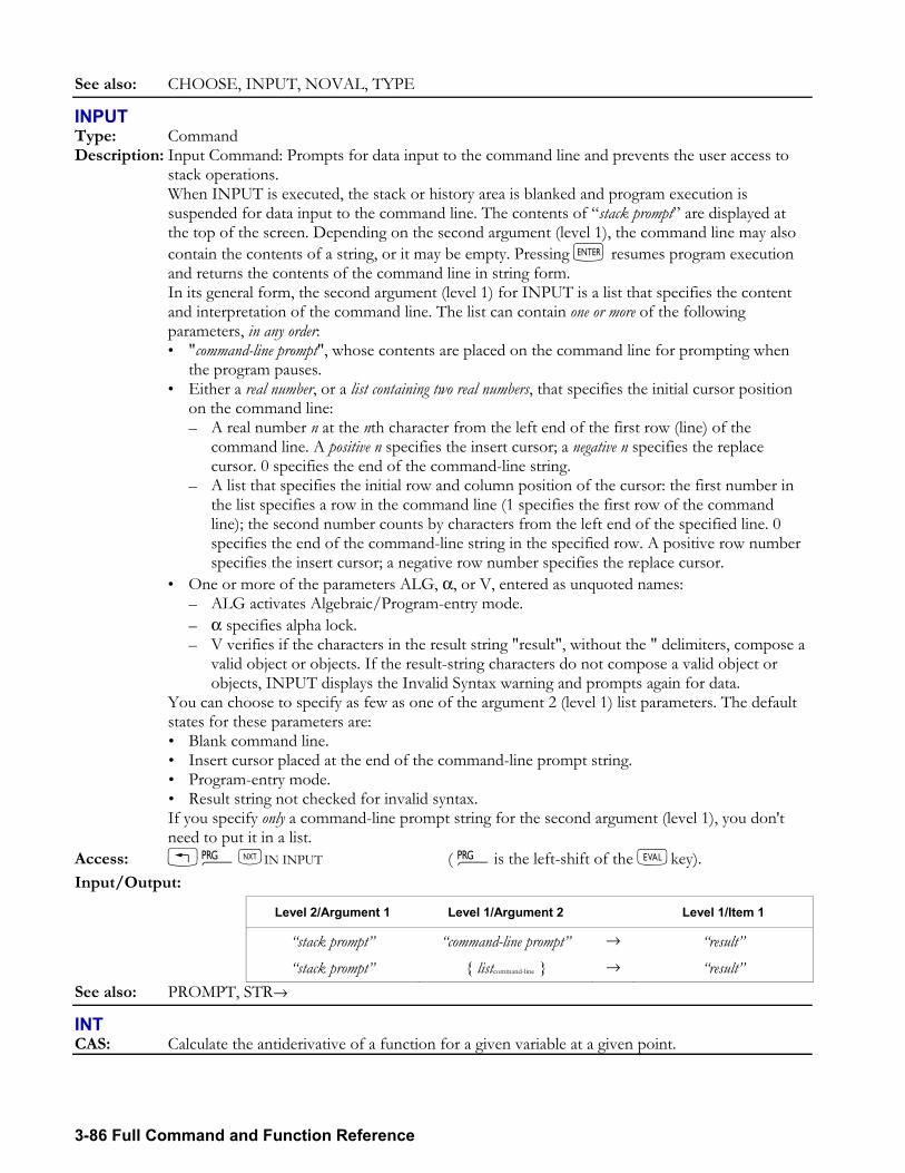
3-86 Full Command and Function Reference
See also: CHOOSE, INPUT, NOVAL, TYPE
INPUT Type: Command Description: Input Command: Prompts for data input to the command line and prevents the user access to
stack operations. When INPUT is executed, the stack or history area is blanked and program execution is
suspended for data input to the command line. The contents of stack prompt are displayed at the top of the screen. Depending on the second argument (level 1), the command line may also contain the contents of a string, or it may be empty. Pressing ` resumes program execution and returns the contents of the command line in string form.
In its general form, the second argument (level 1) for INPUT is a list that specifies the content and interpretation of the command line. The list can contain one or more of the following parameters, in any order: "command-line prompt", whose contents are placed on the command line for prompting when
the program pauses. Either a real number, or a list containing two real numbers, that specifies the initial cursor position
on the command line: A real number n at the nth character from the left end of the first row (line) of the
command line. A positive n specifies the insert cursor; a negative n specifies the replace cursor. 0 specifies the end of the command-line string.
A list that specifies the initial row and column position of the cursor: the first number in the list specifies a row in the command line (1 specifies the first row of the command line); the second number counts by characters from the left end of the specified line. 0 specifies the end of the command-line string in the specified row. A positive row number specifies the insert cursor; a negative row number specifies the replace cursor.
One or more of the parameters ALG, α, or V, entered as unquoted names: ALG activates Algebraic/Program-entry mode. α specifies alpha lock. V verifies if the characters in the result string "result", without the " delimiters, compose a
valid object or objects. If the result-string characters do not compose a valid object or objects, INPUT displays the Invalid Syntax warning and prompts again for data.
You can choose to specify as few as one of the argument 2 (level 1) list parameters. The default states for these parameters are: Blank command line. Insert cursor placed at the end of the command-line prompt string. Program-entry mode. Result string not checked for invalid syntax.
If you specify only a command-line prompt string for the second argument (level 1), you don't need to put it in a list.
Access: !°LIN INPUT ( °is the left-shift of the Nkey). Input/Output:
Level 2/Argument 1 Level 1/Argument 2 Level 1/Item 1
stack prompt command-line prompt → result stack prompt listcommand-line → result
See also: PROMPT, STR→
INT CAS: Calculate the antiderivative of a function for a given variable at a given point.
Full Command and Function Reference 3-87
INTEGER CAS: Display a menu or list of CAS integer operations.
INTVX CAS: Find the antiderivative of a function symbolically, with respect to the current default variable.
INV Type: Analytic function Description: Inverse (1/x) Analytic Function: Returns the reciprocal or the matrix inverse. For a complex argument (x, y), the inverse is the complex number:
x
x2 y2+---------------- y
x2 y2+----------------,
⎝ ⎠⎜ ⎟⎛ ⎞
Matrix arguments must be square (real or complex). The computed inverse matrix A-1 satisfies A
× A-1 = In, where In is the n × n identity matrix. Access: Y
Flags: Numerical Results (3) Input/Output:
Level 1/Argument 1 Level 1/Item 1
z → 1/z [[ matrix ]] → [[ matrix ]]1
'symb' → 'INV(symb)' x_unit → 1/x_1/unit
See also: SINV, /
INVMOD CAS: Perform modular inversion on an object, modulo the current modulus.
IP Type: Function Description: Integer Part Function: Returns the integer part of its argument. The result has the same sign as the argument. Access: !´ REALL IP ( ´ is the left-shift of the Pkey). Flags: Numerical Results (3) Input/Output:
Level 1/Argument 1 Level 1/Item 1
x → n x_unit → n_unit 'symb' → 'IP(symb)'
See also: FP
IQUOT CAS: Return the integer (or Euclidean) quotient of integers a, b; the integer part of a/b.
IREMAINDER CAS: Return the remainder of the division of one integer by another.
ISOL Type: Command
3-88 Full Command and Function Reference
Description: Isolate Variable Command: Returns an algebraic symb2 that rearranges symb1 to isolate the first occurrence of variable global.
The result symb2 is an equation of the form global = expression. If global appears more than once, then symb2 is effectively the right side of an equation obtained by rearranging and solving symb1 to isolate the first occurrence of global on the left side of the equation.
If symb1 is an expression, it is treated as the left side of an equation symb1 = 0. If global appears in the argument of a function within symb1, that function must be an analytic
function, that is, a function for which the hp49g+/hp48gII provides an inverse. Thus ISOL cannot solve IP(x)=0 for x, since IP has no inverse.
ISOL is identical to SOLVE. Access: !ÎISOL ( Îis the left-shift of the 7key). Flags: Principal Solution (-1), Numerical Results (3) Input/Output:
Level 2/Argument 1 Level 1/Argument 2 Level 1/Item 1
'symb1' 'global' → 'symb2' See also: COLCT, EXPAN, QUAD, SHOW, SOLVE
ISOM CAS: Determine the characteristics of a 2-d or 3-d linear isometry.
ISPRIME? CAS: Test if a number is prime. For large numbers test if the number is pseudoprime.
I→R Type: Function Description: Converts an integer into a real number. Access: Ú REWRITE Flags: Exact mode must be set (flag 105 clear). Numeric mode must not be set (flag 3 clear). The
flags affect the output only if the input is not an integer. Input: Level 1/Argument 1: An integer. Output: Level 1/Item 1: The integer converted to a real number. See also: →NUM, R→I, XNUM
JORDAN CAS: Diagonalization, or Jordan cycle decomposition, of a matrix.
KER CAS: Compute the basis of the kernel of a linear application.
KERRM Type: Command Description: Kermit Error Message Command: Returns the text of the most recent Kermit error packet. If a Kermit transfer fails due to an error packet sent from the connected Kermit device to the
hp49g+/hp48gII, then executing KERRM retrieves and displays the error message. (Kermit errors not in packets are retrieved by ERRM rather than KERRM.)
Access: µ KERRM Input/Output:
Level 1/Argument 1 Level 1/Item 1
→ error message
See also: FINISH, KGET, PKT, RECN, RECV, SEND, SERVER
Full Command and Function Reference 3-89
KEY Type: Command Description: Key Command: Returns a test result and, if a key is pressed, returns the row-column location xn
m of that key. KEY returns a false result (0) to item 2 (stack level 1) until a key is pressed. When a key is
pressed, it returns a true result (1) to item 2 (stack level 1) and xn m to item 1 (stack level 2). The result xn m is a two- or three-digit number that identifies the row and column location of the key just pressed. Unlike WAIT, which returns a three-digit number that identifies alpha and shifted keyboard planes, KEY returns the row-column location of any key pressed, including !, , and ~.
Access: !°LIN KEY ( °is the left-shift of the Nkey). Input/Output:
Level 1/Argument 1 Level 2/Item 1 Level 1/Item 2
→ xn m 1
→ 0 See also: WAIT, KEYEVAL
KEYEVAL Type: Command Description: Actions the specified key press. You input a number, in the format ab.c, that represents the key. In the number ab.c:
a is the row coordinate number, where row 1 is the top-most row. b is the column number, where column 1 is the left-most column. c is the shift state of the key, i.e., whether it is normal, alpha-shifted, left shifted, etc. The shift state representations are as follows:
1: Normal function. 2: Left-shift function. 21: Left shift-and-hold function. 3. Right-shift function. 31: Right shift-and-hold function. 4. Alpha-function. 41: Alpha shift-and-hold function. 5. Alpha-left-shift function. 51: Alpha-left-shift-and-hold function. 6. Alpha-right-shift function. 61: Alpha-right-shift-and-hold function.
The sign of the input controls whether USER mode key assignments are used. Positive inputs specify the USER mode key definition. Negative inputs specify the default system keyboard.
Access: µ KEYEVAL Input/Output:
Level 1/Argument 1 Level 1/Item 1
nn.n →
Example: Turn the calculator off using a command. Command: KEYEVAL(101.3) Result: The calculator is turned off.
→KEYTIME Type: Command Description: This command is provided for compatibility with earlier calculators, but does nothing on the
hp49g+/hp48gII.
KEYTIME→ Type: Command Description: This command is provided for compatibility with earlier calculators, but does nothing on the
hp49g+/hp48gII.
3-90 Full Command and Function Reference
KGET Type: Command Description: Kermit Get Command: Used by a local Kermit to get a Kermit server to transmit the named
object(s). To rename an object when the local device gets it, include the old and new names in an
embedded list. For example, AAA BBB KGET gets the variable named AAA but changes its name to BBB. AAA BBB CCC KGET gets AAA as BBB and gets CCC under its own name. (If the original name is not legal on the hp49g+/hp48gII, enter it as a string.)
Access: µ KGET Flags: I/O Device (-33), RECV Overwrite (-36), I/O Messages (-39) Input/Output:
Level 1/Argument 1 Level 1/Item 1
'name' → name →
nameold namenew → name1 ... namen →
nameold namenew name ... → See also: BAUD, CKSM, FINISH, PARITY, RECN, RECV, SEND, SERVER, TRANSIO
KILL Type: Command Description: Cancel Halted Programs Command: Cancels all currently halted programs. If KILL is executed
within a program, that program is also canceled. Canceled programs cannot be resumed. KILL cancels only halted programs and the program from which KILL was executed, if any.
Commands that halt programs are HALT and PROMPT. Suspended programs cannot be canceled. Commands that suspend programs are INPUT and
WAIT. Access: !°LL RUN & DEBUG KILL ( °is the left-shift of the Nkey). Input/Output: None See also: CONT, DOERR, HALT, PROMPT
LABEL Type: Command Description: Label Axes Command: Labels axes in PICT with x- and y-axis variable names and with the
minimum and maximum values of the display ranges. The horizontal axis name is chosen in the following priority order:
1. If the axes parameter in the reserved variable PPAR is a list, then the x-axis element from that list is used.
2. If axes parameter is not a list, then the independent variable name in PPAR is used. The vertical axis name is chosen in the following priority order:
1. If the axes parameter in PPAR is a list, then the y-axis element from that list is used. 2. If axes is not a list, then the dependent variable name from PPAR is used.
Access: µ LABEL Input/Output: None See also: AXES, DRAW, DRAX
LAGRANGE CAS: Return the interpolating polynomial of minimum degree for a set of pairs of values.
Full Command and Function Reference 3-91
LANGUAGE→ Type: Command Description: Language: Returns the language that is currently set. 0 for English, 1 for French, and 2 for
Spanish. Access: µ LANGUAGE→ Input/Output:
Level 1/Argument 1 Level 1/Item 1
→ value
See also: →LANGUAGE
→LANGUAGE Type: Command Description: Language: Sets the language for things such as error messages: 0 for English, 1 for French, and 2
for Spanish. Access: µ →LANGUAGE Input/Output:
Level 1/Argument 1 Level 1/Item 1
value → See also: LANGUAGE→
LAP CAS: Perform a Laplace transform on an expression with respect to the current default variable.
LAPL CAS: Return the Laplacian of a function with respect to a list of variables.
LAST Type: Command Description: Returns copies of the arguments of the most recently executed command. LAST is provided for compatibility with the HP28S. LAST is the same as LASTARG. Access: None. Must be typed in. Flags: Last Arguments (-55) Input/Output:
Level 1 Level n Level 1
→ objn obj1 See also: ANS, LASTARG
LASTARG Type: Command Description: Returns copies of the arguments of the most recently executed command. The objects return to the same stack levels that they originally occupied. Commands that take no
arguments leave the current saved arguments unchanged. When LASTARG follows a command that evaluates an algebraic expression or program, the last arguments saved are from the evaluated algebraic expression or program, not from the original command.
Access: µ LASTARG !°LLERROR LASTA ( °is the left-shift of the Nkey). !îin RPN mode. (îis the left-shift of the`key). Flags: Last Arguments (-55)
3-92 Full Command and Function Reference
Input/Output:
Level 1 Level n Level 1
→ objn obj1 See also: ANS, LAST
LCD→ Description: LCD to Graphics Object Command: Returns the current stack and menu display as a 131 × 80
(on the hp49g+) or 131 × 64 (on the hp48gII) graphics object. Access: !°LGROB LLCD→ ( °is the left-shift of the Nkey). Input/Output:
Level 1/Argument 1 Level 1/Item 1
→ grob See also: →GROB, →LCD
→LCD Type: Command Description: Graphics Object to LCD Command: Displays the specified graphics object with its upper left
pixel in the upper left corner of the display. If the graphics object is larger than 131 × 72 (on the hp49g+) or 131 × 56 (on the hp48gII), it is truncated.
Access: !°LGROB L→LCD ( °is the left-shift of the Nkey). Input/Output:
Level 1/Argument 1 Level 1/Item 1
grob → See also: BLANK, →GROB, LCD→
LCM CAS: Return the least common multiple of two objects.
LCXM CAS: From a program with arguments i, j, build a matrix of specified size, with elements aij .
LDEC CAS: Solve linear differential equation (LDE), or system of first order LDEs, with constant
coefficients.
LEGENDRE CAS: Return the nth degree Legendre polynomial.
LGCD CAS: Return the greatest common divisor of a list of expressions or values.
LIBEVAL Type: Command Description: Evaluate Library Function Command: Evaluates unnamed library functions. WARNING: Use extreme care when executing this function. Using LIBEVAL with
random addresses will almost always cause a memory loss. Do not use this function unless you know what you are doing.
#nfunction is of the form lllfffh, where lll is the library number, and fff the function number. Access: µ LIBEVAL
Full Command and Function Reference 3-93
Input/Output: Level 1/Argument 1 Level 1/Item 1
#nfunction → See also: EVAL, FLASHEVAL, SYSEVAL
LIBS Type: Command Description: Libraries Command: Lists the title, number, and port of each library attached to the current
directory. The title of a library often takes the form LIBRARY-NAME : Description. A library without a title is displayed as " ".
Access: µ LIBS Input/Output:
Level 1/Argument 1 Level 1/Item 1 → title, nlib, nport, ...,title, nlib, nport
See also: ATTACH, DETACH
lim CAS: Return the limit of a function as its argument approaches a specified value.
LIMIT CAS: Return the limit of a function as its argument approaches a specified value. Identical to lim.
LIN CAS: Linearize expressions involving combinations of exponential terms.
LINE Type: Command Operation Description: Draw Line Command: Draws a line in PICT between the input coordinates. Access: !°LPICT LINE ( °is the left-shift of the Nkey). Input/Output:
Level 2/Argument 1 Level 1/Argument 2 Level 1/Item 1
(x1, y1) (x2, y2) →
#n1, #m1 #n2, #m2 → See also: ARC, BOX, TLINE
ΣLINE Type: Command Description: Regression Model Formula Command: Returns an expression representing the best fit line
according to the current statistical model, using X as the independent variable name, and explicit values of the slope and intercept taken from the reserved variable ΣPAR.
For each curve fitting model, the following table indicates the form of the expression returned by ΣLINE, where m is the slope, x is the independent variable, and b is the intercept.
Model Form of Expression
LINFIT mx + b LOGFIT m ln(x) + b
EXPFIT bemx
PWRFIT bxm
Access: µ ΣLINE
3-94 Full Command and Function Reference
Input/Output: Level 1/Argument 1 Level 1/Item 1
→ 'symbformula' See also: BESTFIT, COLΣ, CORR, COV, EXPFIT, LINFIT, LOGFIT, LR, PREDX, PREDY, PWRFIT,
XCOL, YCOL
LINFIT Type: Command Description: Linear Curve Fit Command: Stores LINFIT as the fifth parameter in the reserved variable
ΣPAR, indicating that subsequent executions of LR are to use the linear curve fitting model. LINFIT is the default specification in ΣPAR. Access: µ LINFIT Input/Output: None See also: BESTFIT, EXPFIT, LOGFIT, LR, PWRFIT
LININ Type: Function Description: Linear Test Function: Tests whether an algebraic is structurally linear for a given variable. If any two subexpressions containing a variable (name) are combined only with addition and
subtraction, and any subexpression containing the variable is at most multiplied or divided by another factor not containing the variable, the algebraic (symb) is determined to be linear for that variable. LININ returns a 1 if the algebraic is linear for the variable, and a 0 if not.
Access: !°TEST !«LININ ( °is the left-shift of the Nkey). Input/Output:
Level 2/Argument 1 Level 1/Argument 2 Level 1/Item 1
'symb' 'name' → 0/1
LINSOLVE CAS: Solve a system of linear equations.
LIST→ Type: Command Description: List to Stack Command: Takes a list of n objects and returns each object to a separate level, and
returns the total number of objects to item n+1 (stack level 1). The command OBJ→ also provides this function. Access: µ LIST→ Input/Output:
Level 1/Argument 1 Leveln+1/Item1 ... Level2/Itemn Level1/Itemn+1
obj1, ...,objn → obj1 ... objn n See also: ARRY→, DTAG, EQ→, →LIST, OBJ→, STR→
→LIST Type: Command Description: Stack to List Command: Takes n specified objects and returns a list of those objects. Access: !°TYPE →LIST ( °is the left-shift of the Nkey). !°LIST →LIST ( °is the left-shift of the Nkey).
Full Command and Function Reference 3-95
Input/Output: Leveln+1/Argument1 Level2/Argumentn Level1/Argumentn+1 Level 1/Item 1
obj1 objn n → obj1, ,objn See also: →ARRY, LIST→, →STR, →TAG, →UNIT
∆LIST Type: Command Description: List Differences Command: Returns the first differences of the elements in a list. Adjacent elements in the list must be suitable for mutual subtraction. Access: !´ LIST ∆LIST ( ´ is the left-shift of the Pkey). Input/Output:
Level 1/Argument 1 Level 1/Item 1
list → differences See also: ΣLIST, ΠLIST, STREAM
ΠLIST Type: Command Description: List Product Command: Returns the product of the elements in a list. The elements in the list must be suitable for mutual multiplication. Access: !´ LIST ΠLIST ( ´ is the left-shift of the Pkey). Input/Output:
Level 1/Argument 1 Level 1/Item 1
list → product See also: ΣLIST, ∆LIST, STREAM
ΣLIST Type: Command Description: List Sum Command: Returns the sum of the elements in a list. The elements in the list must be suitable for mutual addition. Access: !´LIST ΣLIST ( ´ is the left-shift of the Pkey). Input/Output:
Level 1/Argument 1 Level 1/Item 1
list → sum See also: ΠLIST, STREAM
LN Type: Analytic function Description: Natural Logarithm Analytic Function: Returns the natural (base e) logarithm of the argument. For x = 0 or (0, 0), an Infinite Result exception occurs, or, if flag 22 is set, MAXR is returned. The inverse of EXP is a relation, not a function, since EXP sends more than one argument to the
same result. The inverse relation for EXP is the general solution: LN(Z)+2*π*i*n1
The function LN is the inverse of a part of EXP, a part defined by restricting the domain of EXP such that: each argument is sent to a distinct result, and each possible result is achieved.
The points in this restricted domain of EXP are called the principal values of the inverse relation. LN in its entirety is called the principal branch of the inverse relation, and the points sent by LN to the boundary of the restricted domain of EXP form the branch cuts of LN.
The principal branch used by the hp49g+/hp48gII for LN was chosen because it is analytic in the regions where the arguments of the real-valued inverse function are defined. The branch cut
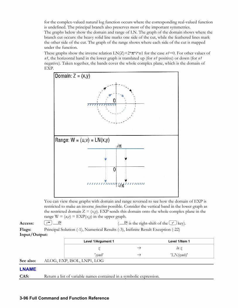
3-96 Full Command and Function Reference
for the complex-valued natural log function occurs where the corresponding real-valued function is undefined. The principal branch also preserves most of the important symmetries.
The graphs below show the domain and range of LN. The graph of the domain shows where the branch cut occurs: the heavy solid line marks one side of the cut, while the feathered lines mark the other side of the cut. The graph of the range shows where each side of the cut is mapped under the function.
These graphs show the inverse relation LN(Z)+2*π*i*n1 for the case n1=0. For other values of n1, the horizontal band in the lower graph is translated up (for n1 positive) or down (for n1 negative). Taken together, the bands cover the whole complex plane, which is the domain of EXP.
You can view these graphs with domain and range reversed to see how the domain of EXP is
restricted to make an inverse function possible. Consider the vertical band in the lower graph as the restricted domain Z = (x,y). EXP sends this domain onto the whole complex plane in the range W = (u,v) = EXP(x,y) in the upper graph.
Access: ¹ (¹is the right-shift of the Qkey). Flags: Principal Solution (-1), Numerical Results (-3), Inifinite Result Exception (-22) Input/Output:
Level 1/Argument 1 Level 1/Item 1
z → ln z 'symb' → 'LN(symb)'
See also: ALOG, EXP, ISOL, LNP1, LOG
LNAME CAS: Return a list of variable names contained in a symbolic expression.
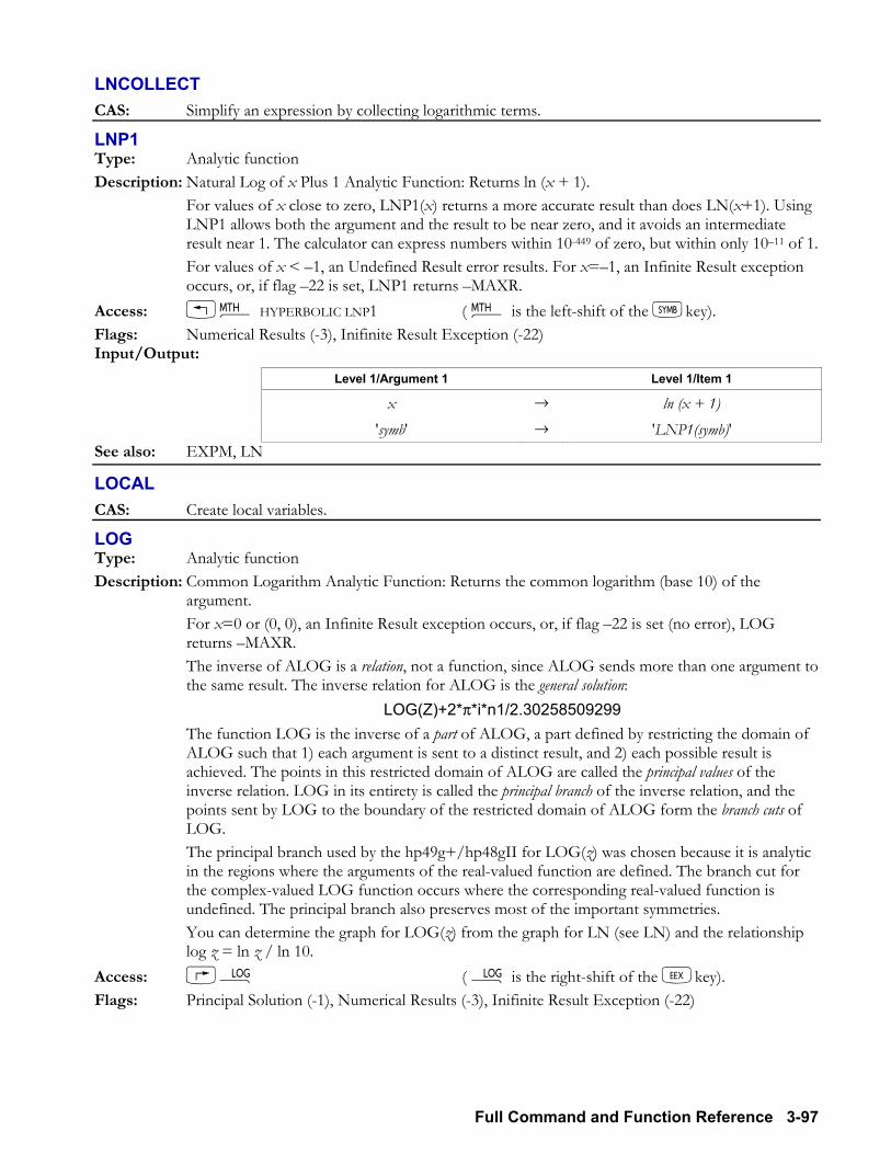
Full Command and Function Reference 3-97
LNCOLLECT CAS: Simplify an expression by collecting logarithmic terms.
LNP1 Type: Analytic function Description: Natural Log of x Plus 1 Analytic Function: Returns ln (x + 1). For values of x close to zero, LNP1(x) returns a more accurate result than does LN(x+1). Using
LNP1 allows both the argument and the result to be near zero, and it avoids an intermediate result near 1. The calculator can express numbers within 10-449 of zero, but within only 1011 of 1.
For values of x < 1, an Undefined Result error results. For x=1, an Infinite Result exception occurs, or, if flag 22 is set, LNP1 returns MAXR.
Access: !´ HYPERBOLIC LNP1 ( ´ is the left-shift of the Pkey). Flags: Numerical Results (-3), Inifinite Result Exception (-22) Input/Output:
Level 1/Argument 1 Level 1/Item 1
x → ln (x + 1) 'symb' → 'LNP1(symb)'
See also: EXPM, LN
LOCAL CAS: Create local variables.
LOG Type: Analytic function Description: Common Logarithm Analytic Function: Returns the common logarithm (base 10) of the
argument. For x=0 or (0, 0), an Infinite Result exception occurs, or, if flag 22 is set (no error), LOG
returns MAXR. The inverse of ALOG is a relation, not a function, since ALOG sends more than one argument to
the same result. The inverse relation for ALOG is the general solution: LOG(Z)+2*π*i*n1/2.30258509299
The function LOG is the inverse of a part of ALOG, a part defined by restricting the domain of ALOG such that 1) each argument is sent to a distinct result, and 2) each possible result is achieved. The points in this restricted domain of ALOG are called the principal values of the inverse relation. LOG in its entirety is called the principal branch of the inverse relation, and the points sent by LOG to the boundary of the restricted domain of ALOG form the branch cuts of LOG.
The principal branch used by the hp49g+/hp48gII for LOG(z) was chosen because it is analytic in the regions where the arguments of the real-valued function are defined. The branch cut for the complex-valued LOG function occurs where the corresponding real-valued function is undefined. The principal branch also preserves most of the important symmetries.
You can determine the graph for LOG(z) from the graph for LN (see LN) and the relationship log z = ln z / ln 10.
Access: Ã ( Ã is the right-shift of the Vkey). Flags: Principal Solution (-1), Numerical Results (-3), Inifinite Result Exception (-22)
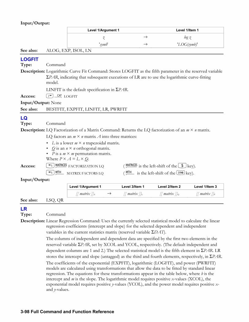
3-98 Full Command and Function Reference
Input/Output: Level 1/Argument 1 Level 1/Item 1
z → log z 'symb' → 'LOG(symb)'
See also: ALOG, EXP, ISOL, LN
LOGFIT Type: Command Description: Logarithmic Curve Fit Command: Stores LOGFIT as the fifth parameter in the reserved variable
ΣPAR, indicating that subsequent executions of LR are to use the logarithmic curve-fitting model.
LINFIT is the default specification in ΣPAR. Access: µ LOGFIT Input/Output: None See also: BESTFIT, EXPFIT, LINFIT, LR, PWRFIT
LQ Type: Command Description: LQ Factorization of a Matrix Command: Returns the LQ factorization of an m × n matrix. LQ factors an m × n matrix A into three matrices:
L is a lower m × n trapezoidal matrix. Q is an n × n orthogonal matrix. P is a m × m permutation matrix.
Where P × A = L × Q. Access: !Ø FACTORIZATION LQ ( Ø is the left-shift of the 5key). !´ MATRIX FACTORS LQ ( ´ is the left-shift of the Pkey). Input/Output:
Level 1/Argument 1 Level 3/Item 1 Level 2/Item 2 Level 1/Item 3
[[ matrix ]]A → [[ matrix ]]L [[ matrix ]]Q [[ matrix ]]P See also: LSQ, QR
LR Type: Command Description: Linear Regression Command: Uses the currently selected statistical model to calculate the linear
regression coefficients (intercept and slope) for the selected dependent and independent variables in the current statistics matrix (reserved variable ΣDAT).
The columns of independent and dependent data are specified by the first two elements in the reserved variable ΣPAR, set by XCOL and YCOL, respectively. (The default independent and dependent columns are 1 and 2.) The selected statistical model is the fifth element in ΣPAR. LR stores the intercept and slope (untagged) as the third and fourth elements, respectively, in ΣPAR.
The coefficients of the exponential (EXPFIT), logarithmic (LOGFIT), and power (PWRFIT) models are calculated using transformations that allow the data to be fitted by standard linear regression. The equations for these transformations appear in the table below, where b is the intercept and m is the slope. The logarithmic model requires positive x-values (XCOL), the exponential model requires positive y-values (YCOL), and the power model requires positive x- and y-values.
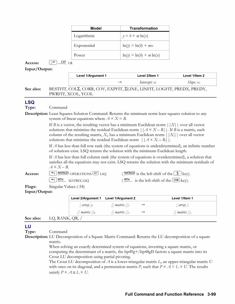
Full Command and Function Reference 3-99
Model Transformation
Logarithmic y = b + m ln(x)
Exponential ln(y) = ln(b) + mx
Power ln(y) = ln(b) + m ln(x)
Access: µ LR Input/Output:
Level 1/Argument 1 Level 2/Item 1 Level 1/Item 2
→ Intercept: x1 Slope: x2 See also: BESTFIT, COLΣ, CORR, COV, EXPFIT, ΣLINE, LINFIT, LOGFIT, PREDX, PREDY,
PWRFIT, XCOL, YCOL
LSQ Type: Command Description: Least Squares Solution Command: Returns the minimum norm least squares solution to any
system of linear equations where A × X = B. If B is a vector, the resulting vector has a minimum Euclidean norm ||X|| over all vector
solutions that minimize the residual Euclidean norm ||A × X B||. If B is a matrix, each column of the resulting matrix, Xi, has a minimum Euclidean norm ||Xi|| over all vector solutions that minimize the residual Euclidean norm ||A × Xi Bi||.
If A has less than full row rank (the system of equations is underdetermined), an infinite number of solutions exist. LSQ returns the solution with the minimum Euclidean length.
If A has less than full column rank (the system of equations is overdetermined), a solution that satisfies all the equations may not exist. LSQ returns the solution with the minimum residuals of A × X B.
Access: !Ø OPERATIONS L LSQ ( Ø is the left-shift of the 5key). !´ MATRIX LSQ ( ´ is the left-shift of the Pkey). Flags: Singular Values (-54) Input/Output:
Level 2/Argument 1 Level 1/Argument 2 Level 1/Item 1
[ array ]B [[ matrix ]]A → [ array ]x
[[ matrix ]]B [[ matrix ]]A → [[ matrix ]]x See also: LQ, RANK, QR, /
LU Type: Command Description: LU Decomposition of a Square Matrix Command: Returns the LU decomposition of a square
matrix. When solving an exactly determined system of equations, inverting a square matrix, or
computing the determinant of a matrix, the hp49g+/hp48gII factors a square matrix into its Crout LU decomposition using partial pivoting.
The Crout LU decomposition of A is a lower-triangular matrix L, an upper-triangular matrix U with ones on its diagonal, and a permutation matrix P, such that P × A = L × U. The results satisfy P × A ≅ L × U.
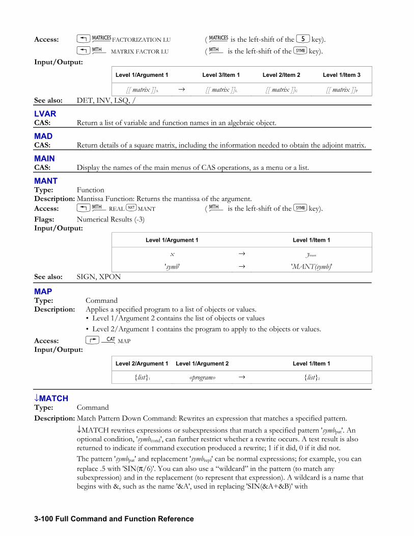
3-100 Full Command and Function Reference
Access: !Ø FACTORIZATION LU ( Ø is the left-shift of the 5key). !´ MATRIX FACTOR LU ( ´ is the left-shift of the Pkey). Input/Output:
Level 1/Argument 1 Level 3/Item 1 Level 2/Item 2 Level 1/Item 3
[[ matrix ]]A → [[ matrix ]]L [[ matrix ]]U [[ matrix ]]P See also: DET, INV, LSQ, /
LVAR CAS: Return a list of variable and function names in an algebraic object.
MAD CAS: Return details of a square matrix, including the information needed to obtain the adjoint matrix.
MAIN CAS: Display the names of the main menus of CAS operations, as a menu or a list.
MANT Type: Function Description: Mantissa Function: Returns the mantissa of the argument. Access: !´REAL LMANT ( ´ is the left-shift of the Pkey). Flags: Numerical Results (-3) Input/Output:
Level 1/Argument 1 Level 1/Item 1
x → ymant
'symb' → 'MANT(symb)' See also: SIGN, XPON
MAP Type: Command Description: Applies a specified program to a list of objects or values.
Level 1/Argument 2 contains the list of objects or values Level 2/Argument 1 contains the program to apply to the objects or values.
Access: µMAP Input/Output:
Level 2/Argument 1 Level 1/Argument 2 Level 1/Item 1
list1 «program» → list2
↓MATCH Type: Command Description: Match Pattern Down Command: Rewrites an expression that matches a specified pattern. ↓MATCH rewrites expressions or subexpressions that match a specified pattern 'symbpat'. An
optional condition, 'symbcond', can further restrict whether a rewrite occurs. A test result is also returned to indicate if command execution produced a rewrite; 1 if it did, 0 if it did not.
The pattern 'symbpat' and replacement 'symbrepl' can be normal expressions; for example, you can replace .5 with 'SIN(π/6)'. You can also use a wildcard in the pattern (to match any subexpression) and in the replacement (to represent that expression). A wildcard is a name that begins with &, such as the name '&A', used in replacing 'SIN(&A+&B)' with
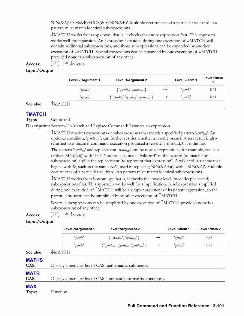
Full Command and Function Reference 3-101
'SIN(&A)*COS(&B)+COS(&A)*SIN(&B)'. Multiple occurrences of a particular wildcard in a pattern must match identical subexpressions.
↓MATCH works from top down; that is, it checks the entire expression first. This approach works well for expansion. An expression expanded during one execution of ↓MATCH will contain additional subexpressions, and those subexpressions can be expanded by another execution of ↓MATCH. Several expressions can be expanded by one execution of ↓MATCH provided none is a subexpression of any other.
Access: µ↓MATCH Input/Output:
Level 2/Argument 1 Level 1/Argument 2 Level 2/Item 1 Level 1/Item 2
'symb1' 'symbpat' 'symbrepl' → 'symb2' 0/1
'symb1' 'symbpat' 'symbrepl' 'symbcond' → 'symb2' 0/1 See also: ↑MATCH
↑MATCH Type: Command Description: Bottom-Up Match and Replace Command: Rewrites an expression. ↑MATCH rewrites expressions or subexpressions that match a specified pattern 'symbpat'. An
optional condition, 'symbcond', can further restrict whether a rewrite occurs. A test result is also returned to indicate if command execution produced a rewrite; 1 if it did, 0 if it did not.
The pattern 'symbpat' and replacement 'symbrepl' can be normal expressions; for example, you can replace 'SIN(π/6)' with '1/2'. You can also use a wildcard in the pattern (to match any subexpression) and in the replacement (to represent that expression). A wildcard is a name that begins with &, such as the name '&A', used in replacing 'SIN(&A+π)' with 'SIN(&A)'. Multiple occurrences of a particular wildcard in a pattern must match identical subexpressions.
↑MATCH works from bottom up; that is, it checks the lowest level (most deeply nested) subexpressions first. This approach works well for simplification. A subexpression simplified during one execution of ↑MATCH will be a simpler argument of its parent expression, so the parent expression can be simplified by another execution of ↑MATCH.
Several subexpressions can be simplified by one execution of ↑MATCH provided none is a subexpression of any other.
Access: µ↑MATCH Input/Output:
Level 2/Argument 1 Level 1/Argument 2 Level 2/Item 1 Level 1/Item 2
'symb1' 'symbpat', 'symbrepl' → 'symb2' 0/1
'symb1' 'symbpat', 'symbrepl', 'symbcond' → 'symb2' 0/1 See also: ↓MATCH
MATHS CAS: Display a menu or list of CAS mathematics submenus.
MATR CAS: Display a menu or list of CAS commands for matrix operations.
MAX Type: Function
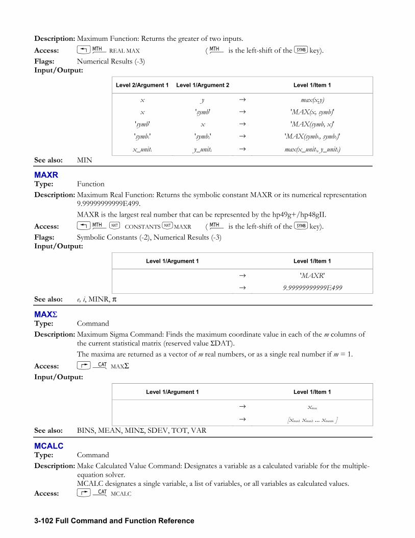
3-102 Full Command and Function Reference
Description: Maximum Function: Returns the greater of two inputs. Access: !´REAL MAX ( ´ is the left-shift of the Pkey). Flags: Numerical Results (-3) Input/Output:
Level 2/Argument 1 Level 1/Argument 2 Level 1/Item 1
x y → max(x,y) x 'symb' → 'MAX(x, symb)'
'symb' x → 'MAX(symb, x)' 'symb1' 'symb2' → 'MAX(symb1, symb2)'
x_unit1 y_unit2 → max(x_unit1, y_unit2) See also: MIN
MAXR Type: Function Description: Maximum Real Function: Returns the symbolic constant MAXR or its numerical representation
9.99999999999E499. MAXR is the largest real number that can be represented by the hp49g+/hp48gII. Access: !´L CONSTANTS LMAXR ( ´ is the left-shift of the Pkey). Flags: Symbolic Constants (-2), Numerical Results (-3) Input/Output:
Level 1/Argument 1 Level 1/Item 1
→ 'MAXR' → 9.99999999999E499
See also: e, i, MINR, π
MAXΣ Type: Command Description: Maximum Sigma Command: Finds the maximum coordinate value in each of the m columns of
the current statistical matrix (reserved value ΣDAT). The maxima are returned as a vector of m real numbers, or as a single real number if m = 1. Access: µ MAXΣ Input/Output:
Level 1/Argument 1 Level 1/Item 1
→ xmax
→ [xmax1 xmax2 ... xmaxm ] See also: BINS, MEAN, MINΣ, SDEV, TOT, VAR
MCALC Type: Command Description: Make Calculated Value Command: Designates a variable as a calculated variable for the multiple-
equation solver. MCALC designates a single variable, a list of variables, or all variables as calculated values. Access: µ MCALC
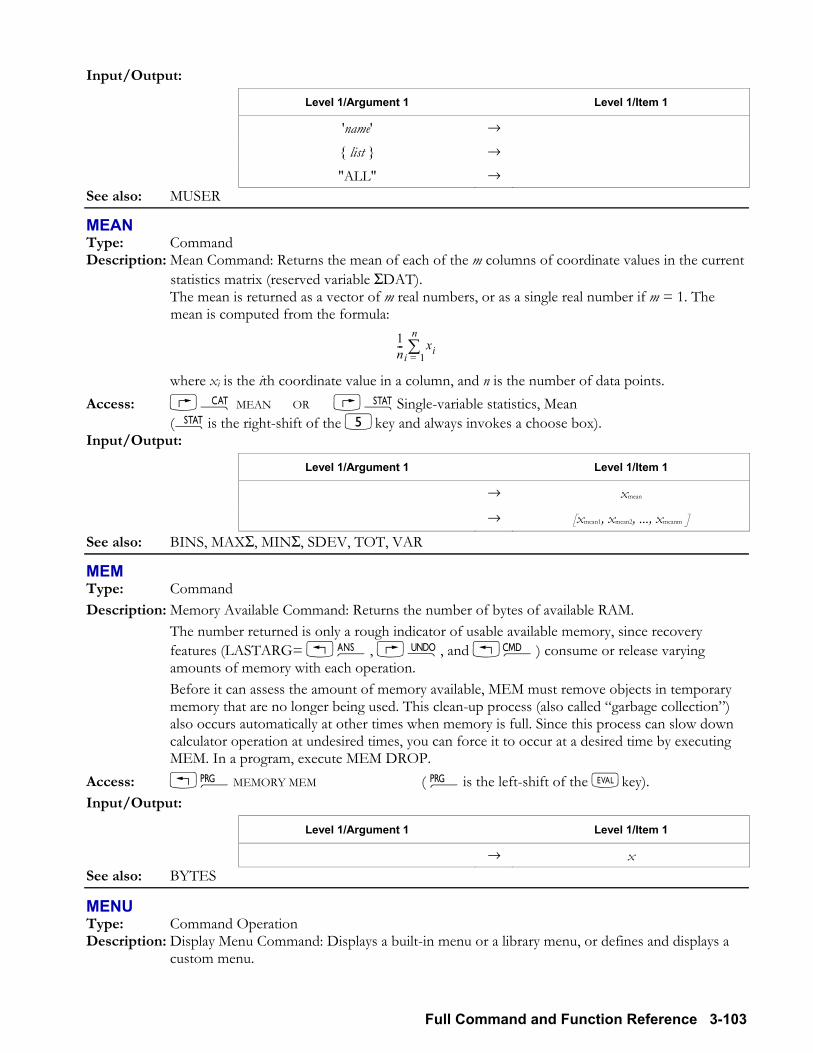
Full Command and Function Reference 3-103
Input/Output:
Level 1/Argument 1 Level 1/Item 1
'name' → list → "ALL" →
See also: MUSER
MEAN Type: Command Description: Mean Command: Returns the mean of each of the m columns of coordinate values in the current
statistics matrix (reserved variable ΣDAT). The mean is returned as a vector of m real numbers, or as a single real number if m = 1. The
mean is computed from the formula: 1n---
xii 1=
n∑
where xi is the ith coordinate value in a column, and n is the number of data points. Access: µ MEAN OR ÙSingle-variable statistics, Mean (Ùis the right-shift of the 5key and always invokes a choose box). Input/Output:
Level 1/Argument 1 Level 1/Item 1
→ xmean
→ [xmean1, xmean2, ..., xmeanm ] See also: BINS, MAXΣ, MINΣ, SDEV, TOT, VAR
MEM Type: Command Description: Memory Available Command: Returns the number of bytes of available RAM. The number returned is only a rough indicator of usable available memory, since recovery
features (LASTARG= !î, ¯, and !®) consume or release varying amounts of memory with each operation.
Before it can assess the amount of memory available, MEM must remove objects in temporary memory that are no longer being used. This clean-up process (also called garbage collection) also occurs automatically at other times when memory is full. Since this process can slow down calculator operation at undesired times, you can force it to occur at a desired time by executing MEM. In a program, execute MEM DROP.
Access: !°MEMORY MEM ( °is the left-shift of the Nkey). Input/Output:
Level 1/Argument 1 Level 1/Item 1
→ x See also: BYTES
MENU Type: Command Operation Description: Display Menu Command: Displays a built-in menu or a library menu, or defines and displays a
custom menu.
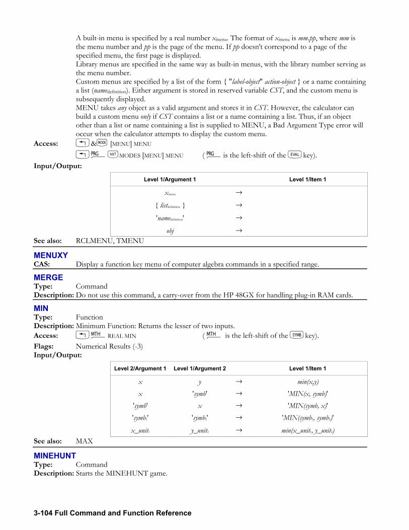
3-104 Full Command and Function Reference
A built-in menu is specified by a real number xmenu. The format of xmenu is mm.pp, where mm is the menu number and pp is the page of the menu. If pp doesn't correspond to a page of the specified menu, the first page is displayed.
Library menus are specified in the same way as built-in menus, with the library number serving as the menu number.
Custom menus are specified by a list of the form "label-object" action-object or a name containing a list (namedefinition). Either argument is stored in reserved variable CST, and the custom menu is subsequently displayed.
MENU takes any object as a valid argument and stores it in CST. However, the calculator can build a custom menu only if CST contains a list or a name containing a list. Thus, if an object other than a list or name containing a list is supplied to MENU, a Bad Argument Type error will occur when the calculator attempts to display the custom menu.
Access: !&H [MENU] MENU !°LMODES [MENU] MENU ( °is the left-shift of the Nkey). Input/Output:
Level 1/Argument 1 Level 1/Item 1
xmenu →
listdefinition →
'namedefinition' →
obj → See also: RCLMENU, TMENU
MENUXY CAS: Display a function key menu of computer algebra commands in a specified range.
MERGE Type: Command Description: Do not use this command, a carry-over from the HP 48GX for handling plug-in RAM cards.
MIN Type: Function Description: Minimum Function: Returns the lesser of two inputs. Access: !´REAL MIN ( ´ is the left-shift of the Pkey). Flags: Numerical Results (-3) Input/Output:
Level 2/Argument 1 Level 1/Argument 2 Level 1/Item 1
x y → min(x,y) x 'symb' → 'MIN(x, symb)'
'symb' x → 'MIN(symb, x)' 'symb1' 'symb2' → 'MIN(symb1, symb2)'
x_unit1 y_unit2 → min(x_unit1, y_unit2) See also: MAX
MINEHUNT Type: Command Description: Starts the MINEHUNT game.
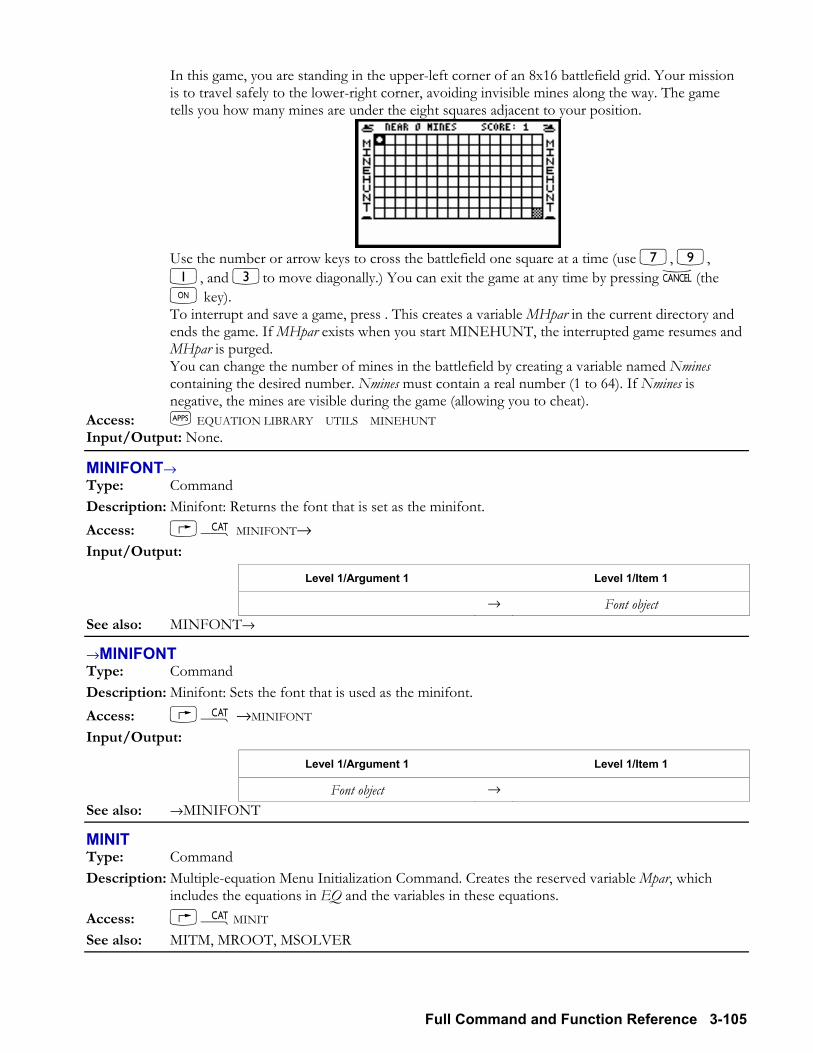
Full Command and Function Reference 3-105
In this game, you are standing in the upper-left corner of an 8x16 battlefield grid. Your mission is to travel safely to the lower-right corner, avoiding invisible mines along the way. The game tells you how many mines are under the eight squares adjacent to your position.
Use the number or arrow keys to cross the battlefield one square at a time (use 7, 9,
1, and 3to move diagonally.) You can exit the game at any time by pressing −(the $ key).
To interrupt and save a game, press . This creates a variable MHpar in the current directory and ends the game. If MHpar exists when you start MINEHUNT, the interrupted game resumes and MHpar is purged.
You can change the number of mines in the battlefield by creating a variable named Nmines containing the desired number. Nmines must contain a real number (1 to 64). If Nmines is negative, the mines are visible during the game (allowing you to cheat).
Access: G EQUATION LIBRARY UTILS MINEHUNT Input/Output: None.
MINIFONT→ Type: Command Description: Minifont: Returns the font that is set as the minifont. Access: µ MINIFONT→ Input/Output:
Level 1/Argument 1 Level 1/Item 1
→ Font object See also: MINFONT→
→MINIFONT Type: Command Description: Minifont: Sets the font that is used as the minifont. Access: µ →MINIFONT Input/Output:
Level 1/Argument 1 Level 1/Item 1
Font object → See also: →MINIFONT
MINIT Type: Command Description: Multiple-equation Menu Initialization Command. Creates the reserved variable Mpar, which
includes the equations in EQ and the variables in these equations. Access: µMINIT See also: MITM, MROOT, MSOLVER
3-106 Full Command and Function Reference
MINR Type: Function Description: Minimum Real Function: Returns the symbolic constant MINR or its numerical representation,
1.00000000000E499. MINR is the smallest positive real number that can be represented by the hp49g+/hp48gII. Access: !´LCONSTANTS LMINR ( ´ is the left-shift of the Pkey). Flags: Symbolic Constants (-2), Numerical Results (-3) Input/Output:
Level 1/Argument 1 Level 1/Item 1
→ 'MINR' → 1.00000000000E499
See also: e, i, MAXR, π
MINΣ Type: Command Description: Minimum Sigma Command: Finds the minimum coordinate value in each of the m columns of
the current statistics matrix (reserved variable ΣDAT). The minima are returned as a vector of m real numbers, or as a single real number if m = 1. Access: µ MINΣ Input/Output:
Level 1/Argument 1 Level 1/Item 1
→ xmin
→ xmin 1 xmin 2 xmin m See also: BINS, MAXΣ, MEAN, SDEV, TOT, VAR
MITM Type: Command Description: Multiple-equation Menu Item Order Command. Changes multiple equation menu titles and
order. The argument list contains the variable names in the order you want. Use "" to indicate a blank label. You must include all variables in the original menu and no others.
Access: µMITM Input/Output:
Level 2/Argument 1 Level 1/Argument 2 Level 1/Item 1
"title" list → See also: MINIT
MKISOM CAS: Return the matrix representation for a given isometry.
MOD Type: Function Description: Modulo Function: Returns a remainder defined by: x mod y = x y floor (x/y) Mod (x, y) is periodic in x with period y. Mod (x, y) lies in the interval [0, y) for y > 0 and in (y, 0]
for y < 0. Algebraic syntax: argument 1 MOD argument 2 Access: !´REAL MOD ( ´ is the left-shift of the Pkey). !ÞMODUL L MOD ( Þ is the left-shift of the 1key).
Full Command and Function Reference 3-107
Flags: Numerical Results (-3) Input/Output:
Level 2/Argument 1 Level 1/Argument 2 Level 1/Item 1
x y → x mod y x 'symb' → 'MOD(x, symb)'
'symb' x → 'MOD(symb, x)' 'symb1' 'symb2' → 'MOD(symb1, symb2)'
See also: FLOOR, /
MODSTO CAS: Change the modulo setting to the specified number.
MODULAR CAS: Display a menu or list of CAS modulo operations.
MROOT Type: Command Description: Multiple Roots Command: Uses the multiple-equation solver to solve for one or more variables
using the equations in EQ. Given a variable name, MROOT returns the found value; with "ALL" MROOT stores a found value for each variable but returns nothing.
Access: µ MROOT Input/Output:
Level 1/Argument 1 Level 1/Item 1
'name' → x "ALL" →
See also: MCALC, MUSER
MSGBOX Type: Command Description: Message Box Command: Creates a user-defined message box. MSGBOX displays message in the form of a standard message box. Message text too long to
appear on the screen is truncated. You can use spaces and new-line characters (ë) to control word-wrapping and line breaks within the message.
Program execution resumes when the message box is exited by selecting OK or CANCL. Access: !°LOUT MSGBOX ( °is the left-shift of the Nkey). Input/Output:
Level 1/Argument 1 Level 1/Item 1
message → See also: CHOOSE, INFORM, PROMPT
MSLV CAS: Multiple equation solver; numerically approximate a solution to a system of equations.
MSOLVR Type: Command Description: Multiple Equation Solver Command: Gets the multiple-equation solver variable menu for the set
of equations stored in EQ.
3-108 Full Command and Function Reference
The multiple-equation solver application can solve a set of of two or more equations for unknown variables by finding the roots of each equation. The solver uses the list of equations stored in EQ.
Access: µ MSOLVR Input/Output: None See also: EQNLIB, MCALC, MINIT, MITM, MROOT, MSLV, MUSER
MULTMOD CAS: Perform modular multiplication of two objects, modulo the current modulus.
MUSER Type: Command Description: Make User-Defined Variable Command: Designates a variable as user-defined for the multiple-
equation solver. MUSER designates a single variable, a list of variables, or all variables as user-defined. Access: µ MUSER Input/Output:
Level 1/Argument 1 Level 1/Item 1
'name' → list → "ALL" →
See also: MCALC
→NDISP Type: Command Description: Sets the number of program lines displayed on the screen.
The default value on the hp49g+/hp48gII is 9. On the hp49g+ a value of 12 should be set for →NDISP, which will allow more of the hp49g+s taller screen to be used when the font is FONT7, FONT6, or the MINIFONT. Also, note that the →NDISP setting is reset to 9 at every warmstart. Including << 12 →NDISP >> in 'STARTUP' will automatically reset the value to 12.
Access: µ →NDISP Input/Output:
Level 1/Argument 1 Level 1/Item 1
n →
NDIST Type: Command Description: Normal Distribution Command: Returns the normal probability distribution (bell curve) at x
based on the mean m and variance v of the normal distribution. NDIST is calculated using this formula:
ndist m v x, ,( ) e
x m( )2
2v-------------------
2πv---------------------=
Access: !´LPROBABILITY L NDIST ( ´ is the left-shift of the Pkey).
Full Command and Function Reference 3-109
Input/Output: Level 3/Argument 1 Level 2/Argument 2 Level 1/Argument 3 Level 1/Item 1
m v x → ndist(m, v, x) See also: UTPN
NDUPN Type: RPL command Description: Duplicates an object n times, and returns n. Access: !°STACK !«NDUPN ( °is the left-shift of the Nkey).
ISTACK !«NDUPN Input/Output:
Level 2 Level 1 Leveln+1 … Level2 Level1
obj n → obj obj n See also: DUP, DUPDUP, DUPN, DUP2
NEG Type: Analytic function Description: Negate Analytic Function: Changes the sign or negates an object. Negating an array creates a new array containing the negative of each of the original elements.
Negating a binary number takes its two's complement (complements each bit and adds 1). Negating a graphics object inverts it (toggles each pixel from on to off, or vice-versa). If the
argument is PICT, the graphics object stored in PICT is inverted. Access: ß NEG ( ß is the right-shift of the 1key). !´L COMPLEX L NEG ( ´ is the left-shift of the Pkey). W Flags: Numerical Results (-3), Binary Integer Wordsize (-5 through -10) Input/Output:
Level 1/Argument 1 Level 1/Item 1
z → z #n1 → #n2
[ array ] → [ array ] 'symb' → '(symb)' x_unit → x_unit grob1 → grob2
PICT1 → PICT2 See also: ABS, CONJ, NOT, SIGN
NEWOB Type: Command Description: New Object Command: Creates a new copy of the specified object. NEWOB has two main uses:
NEWOB enables the purging of a library or backup object that has been recalled from a port. NEWOB creates a new, separate copy of the object in memory, thereby allowing the original copy to be purged.
3-110 Full Command and Function Reference
Creating a new copy of an object that originated in a larger composite object (such as a list) allows you to recover the memory associated with the larger object when that larger object is no longer needed.
Access: !°MEMORY NEWOB ( °is the left-shift of the Nkey). Flags: Last Arguments (-55). In order for NEWOB to immediately release the memory occupied by the
original copy, flag -55 must be set so that the copy is not saved as a last argument. Input/Output:
Level 1/Argument 1 Level 1/Item 1
obj → obj See also: MEM, PURGE
NEXT Type: Command Description: NEXT Command: Ends definite loop structures. See the FOR and START keyword entries for more information. Access: !°BRANCH START/FOR NEXT ( °is the left-shift of the Nkey). Input/Output: None See also: FOR, START, STEP
NEXTPRIME CAS: Return the next prime number larger than a given integer.
NIP Type: RPL command Description: Drops the (n1)th argument, where n is the number of arguments or items on the stack. (that is,
the object on level 2 of the stack). This is equivalent to executing SWAP folowed by DROP in RPN mode.
Access: !° STACK LLNIP ( °is the left-shift of the Nkey). I STACK LLNIP Input/Output:
Level 2 Level 1 Level 1
obj1 obj2 → obj2 See also: DUP, DUPDUP, DUPN, DUP2
NOT Type: Function Description: NOT Command: Returns the one's complement or logical inverse of the argument. When the argument is a binary integer or string, NOT complements each bit in the argument to
produce the result. A binary integer is treated as a sequence of bits as long as the current wordsize. A string is treated as a sequence of bits, using 8 bits per character (that is, using the binary
version of the character code). When the argument is a real number or symbolic, NOT does a true/false test. The result is 1
(true) if the argument is zero; it is 0 (false) if the argument is nonzero. This test is usually done on a test result (T/F).
If the argument is an algebraic object, then the result is an algebraic of the form NOT symb. Execute →NUM (or set flag 3 before executing NOT) to produce a numeric result from the algebraic result.
Full Command and Function Reference 3-111
Access: !° TEST LNOT ( °is the left-shift of the Nkey). ãL LOGIC NOT (ã is the right-shift of the 3key). Flags: Numerical Results (-3), Binary Integer Wordsize (-5 through -10) Input/Output:
Level 1/Argument 1 Level 1/Item 1
#n1 → #n2
T/F → 0/1 string1 → string2
'symb' → 'NOT symb' See also: AND, OR, XOR
NOVAL Type: Command Description: INFORM Place Holder/Result Command: Place holder for reset and initial values in user-
defined dialog boxes. NOVAL is returned when a field is empty. NOVAL is used to mark an empty field in a user-defined dialog box created with the INFORM
command. INFORM defines fields sequentially. If default values are used for those fields, the defaults must be defined in the same order as the fields were defined. To skip over (not provide defaults for) some of the fields, use the NOVAL command.
After INFORM terminates, NOVAL is returned if a field is empty and OK or ` is selected. Access: !°L IN NOVAL ( °is the left-shift of the Nkey). Input/Output: None See also: INFORM
NΣ Type: Command Description: Number of Rows Command: Returns the number of rows in the current statistical matrix
(reserved variable ΣDAT). Access: µ NΣ Input/Output:
Level 1/Argument 1 Level 1/Item 1
→ nrows See also: ΣX, ΣXY, ΣX2, ΣY, ΣY2
NSUB Type: Command Description: Number of Sublist Command: Provides a way to access the current sublist position during an
iteration of a program or command applied using DOSUBS. Returns an Undefined Local Name error if executed when DOSUBS is not active. Access: !°LIST PROCEDURES NSUB ( °is the left-shift of the Nkey). Input/Output:
Level 1/Argument 1 Level 1/Item 1
→ nposition See also: DOSUBS, ENDSUB
→NUM Type: Command
3-112 Full Command and Function Reference
Description: Evaluate to Number Command. Evaluates a symbolic argument object (other than a list) and returns the numerical result.
→NUM repeatedly evaluates a symbolic argument until a numerical result is achieved. The effect is the same as evaluating a symbolic argument in Numerical Result Mode (flag -3 set).
Access: →NUM (→NUM is the right-shift of the `key). Input/Output:
Level 1/Argument 1 Level 1/Item 1
objsymb → z See also: EVAL
NUM Type: Command Description: Character Number Command: Returns the character code n for the first character in the string. The character codes are an extension of ISO 8859/1. The number of a character can be found by accessing the Characters tool (±) and
highlighting that character. The number appears near the bottom of the screen. Access: !°TYPE LNUM ( °is the left-shift of the Nkey). !° LCHARS NUM ( °is the left-shift of the Nkey). &N NUM Input/Output:
Level 1/Argument 1 Level 1/Item 1
string → n See also: CHR, POS, REPL, SIZE, SUB
NUMX Type: Command Description: Number of X-Steps Command: Sets the number of x-steps for each y-step in 3D perspective
plots. The number of x-steps is the number of independent variable points plotted for each dependent
variable point plotted. This number must be 2 or more. This value is stored in the reserved variable VPAR. YSLICE is the only 3D plot type that does not use this value.
Access: µ NUMX Input/Output:
Level 1/Argument 1 Level 1/Item 1
nx → See also: NUMY
NUMY Type: Command Description: Number of Y-Steps Command: Sets the number of y-steps across the view volume in 3D
perspective plots. The number of y-steps is the number of dependent variable points plotted across the view
volume. This number must be 2 or more. This value is stored in the reserved variable VPAR. Access: µ NUMY Input/Output:
Level 1/Argument 1 Level 1/Item 1
ny →
See also: NUMX
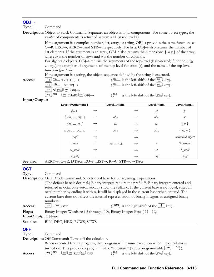
Full Command and Function Reference 3-113
OBJ→ Type: Command Description: Object to Stack Command: Separates an object into its components. For some object types, the
number of components is returned as item n+1 (stack level 1). If the argument is a complex number, list, array, or string, OBJ→ provides the same functions as
C→R, LIST→, ARRY→, and STR→, respectively. For lists, OBJ→ also returns the number of list elements. If the argument is an array, OBJ→ also returns the dimensions m n of the array, where m is the number of rows and n is the number of columns.
For algebraic objects, OBJ→ returns the arguments of the top-level (least-nested) function (arg1 argn), the number of arguments of the top-level function (n), and the name of the top-level function (function).
If the argument is a string, the object sequence defined by the string is executed. Access: !°TYPE OBJ→ ( °is the left-shift of the Nkey). !°LIST OBJ→ ( °is the left-shift of the Nkey). &NL OBJ→ !°LCHARS LOBJ→ ( °is the left-shift of the Nkey). Input/Output:
Level 1/Argument 1 Leveln+1/Item1 Level2/Itemn Level1/Itemn+1 (x, y) → → x y
obj1, ... ,objn → obj1 → objn n
[ x1, ... ,xn ] → x1 → xn n
[[ x1 1, ... ,xm n ]] → x1 1 → xm n m, n
obj → → evaluated object 'symb' → arg1 ... argn → n 'function'
x_unit → → x 1_unit :tag:obj → → obj tag
See also: ARRY→, C→R, DTAG, EQ→, LIST→, R→C, STR→, →TAG
OCT Type: Command Description: Octal Mode Command: Selects octal base for binary integer operations. (The default base is decimal.) Binary integers require the prefix #. Binary integers entered and
returned in octal base automatically show the suffix o. If the current base is not octal, enter an octal number by ending it with o. It will be displayed in the current base when entered. The current base does not affect the internal representation of binary integers as unsigned binary numbers.
Access: ãOCT (ã is the right-shift of the 3key). Flags: Binary Integer Wordsize (-5 through -10), Binary Integer Base (-11, -12) Input/Output: None See also: BIN, DEC, HEX, RCWS, STWS
OFF Type: Command Description: Off Command: Turns off the calculator. When executed from a program, that program will resume execution when the calculator is
turned on. This provides a programmable autostart. ( i.e., a programmable ç). Access: °LLRUNL OFF ( °is the left-shift of the Nkey).
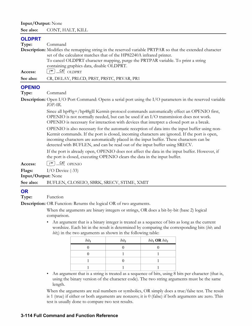
3-114 Full Command and Function Reference
Input/Output: None See also: CONT, HALT, KILL
OLDPRT Type: Command Description: Modifies the remapping string in the reserved variable PRTPAR so that the extended character
set of the calculator matches that of the HP82240A infrared printer. To cancel OLDPRT character mapping, purge the PRTPAR variable. To print a string
containing graphics data, disable OLDPRT. Access: µ OLDPRT See also: CR, DELAY, PRLCD, PRST, PRSTC, PRVAR, PR1
OPENIO Type: Command Description: Open I/O Port Command: Opens a serial port using the I/O parameters in the reserved variable
IOPAR. Since all hp49g+/hp48gII Kermit-protocol commands automatically effect an OPENIO first,
OPENIO is not normally needed, but can be used if an I/O transmission does not work. OPENIO is necessary for interaction with devices that interpret a closed port as a break.
OPENIO is also necessary for the automatic reception of data into the input buffer using non-Kermit commands. If the port is closed, incoming characters are ignored. If the port is open, incoming characters are automatically placed in the input buffer. These characters can be detected with BUFLEN, and can be read out of the input buffer using SRECV.
If the port is already open, OPENIO does not affect the data in the input buffer. However, if the port is closed, executing OPENIO clears the data in the input buffer.
Access: µ OPENIO Flags: I/O Device (-33) Input/Output: None See also: BUFLEN, CLOSEIO, SBRK, SRECV, STIME, XMIT
OR Type: Function Description: OR Function: Returns the logical OR of two arguments. When the arguments are binary integers or strings, OR does a bit-by-bit (base 2) logical
comparison. An argument that is a binary integer is treated as a sequence of bits as long as the current
wordsize. Each bit in the result is determined by comparing the corresponding bits (bit1 and bit2) in the two arguments as shown in the following table:
bit1 bit2 bit1 OR bit2
0 0 0 0 1 1
1 0 1
1 1 1 An argument that is a string is treated as a sequence of bits, using 8 bits per character (that is,
using the binary version of the character code). The two string arguments must be the same length.
When the arguments are real numbers or symbolics, OR simply does a true/false test. The result is 1 (true) if either or both arguments are nonzero; it is 0 (false) if both arguments are zero. This test is usually done to compare two test results.
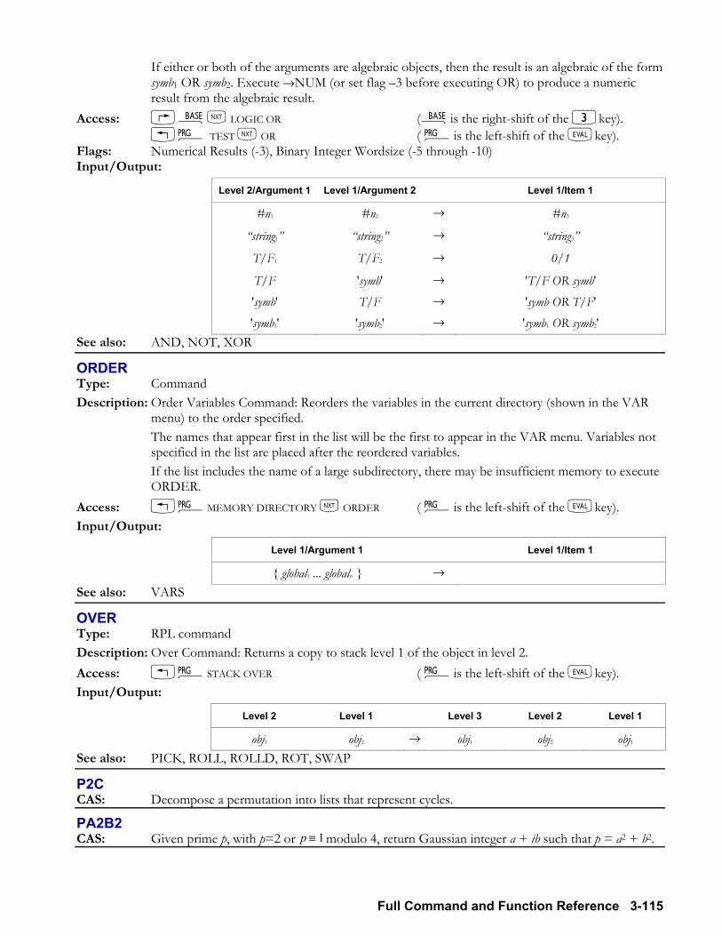
Full Command and Function Reference 3-115
If either or both of the arguments are algebraic objects, then the result is an algebraic of the form symb1 OR symb2. Execute →NUM (or set flag 3 before executing OR) to produce a numeric result from the algebraic result.
Access: ãL LOGIC OR (ãis the right-shift of the 3key). !° TEST L OR ( °is the left-shift of the Nkey). Flags: Numerical Results (-3), Binary Integer Wordsize (-5 through -10) Input/Output:
Level 2/Argument 1 Level 1/Argument 2 Level 1/Item 1
#n1 #n2 → #n3
string1 string2 → string3
T/F1 T/F2 → 0/1
T/F 'symb' → 'T/F OR symb' 'symb' T/F → 'symb OR T/F' 'symb1' 'symb2' → 'symb1 OR symb2'
See also: AND, NOT, XOR
ORDER Type: Command Description: Order Variables Command: Reorders the variables in the current directory (shown in the VAR
menu) to the order specified. The names that appear first in the list will be the first to appear in the VAR menu. Variables not
specified in the list are placed after the reordered variables. If the list includes the name of a large subdirectory, there may be insufficient memory to execute
ORDER. Access: !°MEMORY DIRECTORY L ORDER ( °is the left-shift of the Nkey). Input/Output:
Level 1/Argument 1 Level 1/Item 1
global1 ... globaln → See also: VARS
OVER Type: RPL command Description: Over Command: Returns a copy to stack level 1 of the object in level 2. Access: !°STACK OVER ( °is the left-shift of the Nkey). Input/Output:
Level 2 Level 1 Level 3 Level 2 Level 1
obj1 obj2 → obj1 obj2 obj1 See also: PICK, ROLL, ROLLD, ROT, SWAP
P2C CAS: Decompose a permutation into lists that represent cycles.
PA2B2 CAS: Given prime p, with p=2 or modulo 4, return Gaussian integer a + ib such that p = a2 + b2.
p 1≡
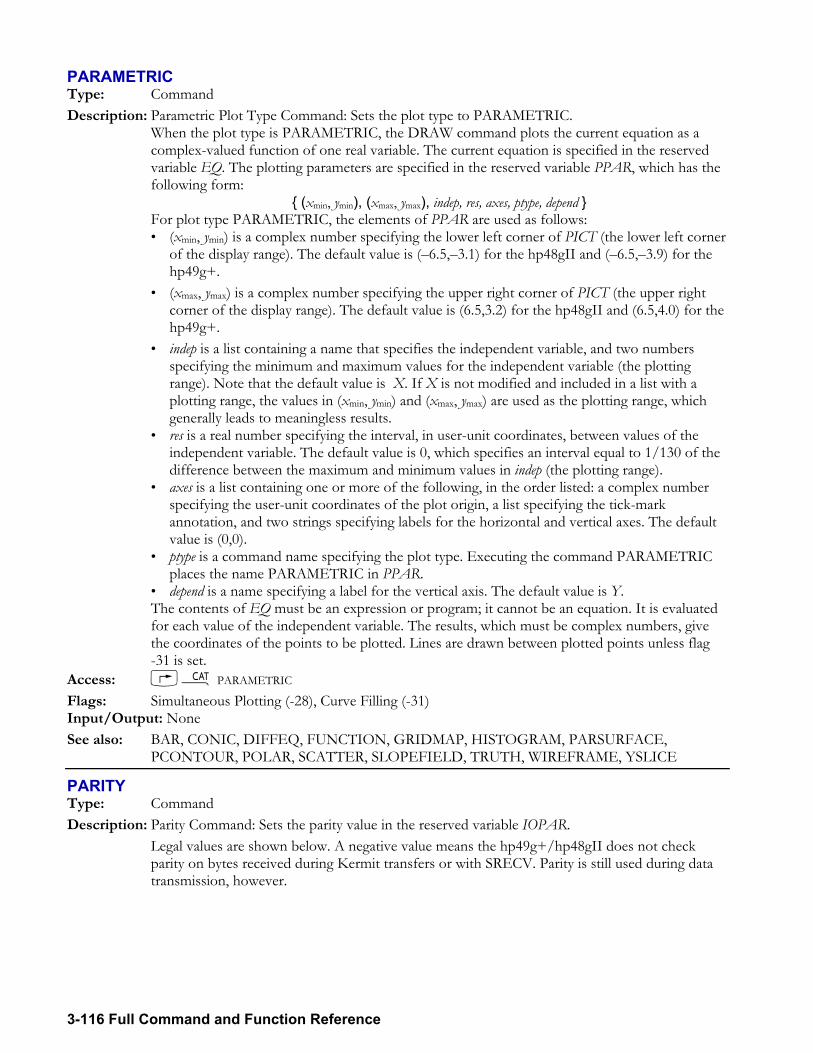
3-116 Full Command and Function Reference
PARAMETRIC Type: Command Description: Parametric Plot Type Command: Sets the plot type to PARAMETRIC. When the plot type is PARAMETRIC, the DRAW command plots the current equation as a
complex-valued function of one real variable. The current equation is specified in the reserved variable EQ. The plotting parameters are specified in the reserved variable PPAR, which has the following form:
(xmin, ymin), (xmax, ymax), indep, res, axes, ptype, depend For plot type PARAMETRIC, the elements of PPAR are used as follows:
(xmin, ymin) is a complex number specifying the lower left corner of PICT (the lower left corner of the display range). The default value is (6.5,3.1) for the hp48gII and (6.5,3.9) for the hp49g+.
(xmax, ymax) is a complex number specifying the upper right corner of PICT (the upper right corner of the display range). The default value is (6.5,3.2) for the hp48gII and (6.5,4.0) for the hp49g+.
indep is a list containing a name that specifies the independent variable, and two numbers specifying the minimum and maximum values for the independent variable (the plotting range). Note that the default value is X. If X is not modified and included in a list with a plotting range, the values in (xmin, ymin) and (xmax, ymax) are used as the plotting range, which generally leads to meaningless results.
res is a real number specifying the interval, in user-unit coordinates, between values of the independent variable. The default value is 0, which specifies an interval equal to 1/130 of the difference between the maximum and minimum values in indep (the plotting range).
axes is a list containing one or more of the following, in the order listed: a complex number specifying the user-unit coordinates of the plot origin, a list specifying the tick-mark annotation, and two strings specifying labels for the horizontal and vertical axes. The default value is (0,0).
ptype is a command name specifying the plot type. Executing the command PARAMETRIC places the name PARAMETRIC in PPAR.
depend is a name specifying a label for the vertical axis. The default value is Y. The contents of EQ must be an expression or program; it cannot be an equation. It is evaluated
for each value of the independent variable. The results, which must be complex numbers, give the coordinates of the points to be plotted. Lines are drawn between plotted points unless flag -31 is set.
Access: µ PARAMETRIC Flags: Simultaneous Plotting (-28), Curve Filling (-31) Input/Output: None See also: BAR, CONIC, DIFFEQ, FUNCTION, GRIDMAP, HISTOGRAM, PARSURFACE,
PCONTOUR, POLAR, SCATTER, SLOPEFIELD, TRUTH, WIREFRAME, YSLICE
PARITY Type: Command Description: Parity Command: Sets the parity value in the reserved variable IOPAR. Legal values are shown below. A negative value means the hp49g+/hp48gII does not check
parity on bytes received during Kermit transfers or with SRECV. Parity is still used during data transmission, however.
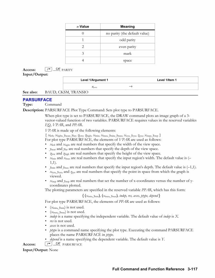
Full Command and Function Reference 3-117
n-Value Meaning
0 no parity (the default value) 1 odd parity
2 even parity
3 mark
4 space
Access: µPARITY Input/Output:
Level 1/Argument 1 Level 1/Item 1
nparity → See also: BAUD, CKSM, TRANSIO
PARSURFACE Type: Command Description: PARSURFACE Plot Type Command: Sets plot type to PARSURFACE. When plot type is set to PARSURFACE, the DRAW command plots an image graph of a 3-
vector-valued function of two variables. PARSURFACE requires values in the reserved variables EQ, VPAR, and PPAR.
VPAR is made up of the following elements: xleft, xright, ynear, yfar, zlow, zhigh, xmin, xmax, ymin, ymax, xeye, yeye, zeye, xstep, ystep For plot type PARSURFACE, the elements of VPAR are used as follows:
xleft and xright are real numbers that specify the width of the view space. ynear and yfar are real numbers that specify the depth of the view space. zlow and zhigh are real numbers that specify the height of the view space. xmin and xmax are real numbers that specify the input region's width. The default value is (
1,1). ymin and ymax are real numbers that specify the input region's depth. The default value is (1,1). xeye, yeye, and zeye are real numbers that specify the point in space from which the graph is
viewed. xstep and ystep are real numbers that set the number of x-coordinates versus the number of y-
coordinates plotted. The plotting parameters are specified in the reserved variable PPAR, which has this form:
(xmin, ymin), (xmax, ymax), indep, res, axes, ptype, depend For plot type PARSURFACE, the elements of PPAR are used as follows:
(xmin, ymin) is not used. (xmax, ymax) is not used. indep is a name specifying the independent variable. The default value of indep is X. res is not used. axes is not used. ptype is a command name specifying the plot type. Executing the command PARSURFACE
places the name PARSURFACE in ptype. depend is a name specifying the dependent variable. The default value is Y.
Access: µ PARSURFACE Input/Output: None
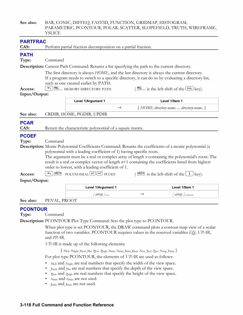
3-118 Full Command and Function Reference
See also: BAR, CONIC, DIFFEQ, FAST3D, FUNCTION, GRIDMAP, HISTOGRAM, PARAMETRIC, PCONTOUR, POLAR, SCATTER, SLOPEFIELD, TRUTH, WIREFRAME, YSLICE
PARTFRAC CAS: Perform partial fraction decomposition on a partial fraction.
PATH Type: Command Description: Current Path Command: Returns a list specifying the path to the current directory. The first directory is always HOME, and the last directory is always the current directory. If a program needs to switch to a specific directory, it can do so by evaluating a directory list,
such as one created earlier by PATH. Access: !°MEMORY DIRECTORY PATH ( °is the left-shift of the Nkey). Input/Output:
Level 1/Argument 1 Level 1/Item 1 → HOME directory-name1 ... directory-namen
See also: CRDIR, HOME, PGDIR, UPDIR
PCAR CAS: Return the characteristic polynomial of a square matrix.
PCOEF Type: Command Description: Monic Polynomial Coefficients Command: Returns the coefficients of a monic polynomial (a
polynomial with a leading coefficient of 1) having specific roots. The argument must be a real or complex array of length n containing the polynomial's roots. The
result is a real or complex vector of length n+1 containing the coefficients listed from highest order to lowest, with a leading coefficient of 1.
Access: !Þ POLYNOMIAL LL PCOEF ( Þis the left-shift of the 1key). Input/Output:
Level 1/Argument 1 Level 1/Item 1
[ array ]roots → [ array ]coefficients See also: PEVAL, PROOT
PCONTOUR Type: Command Description: PCONTOUR Plot Type Command: Sets the plot type to PCONTOUR. When plot type is set PCONTOUR, the DRAW command plots a contour-map view of a scalar
function of two variables. PCONTOUR requires values in the reserved variables EQ, VPAR, and PPAR.
VPAR is made up of the following elements: xleft xright ynear yfar zlow zhigh xmin xmax ymin ymax xeye yeye zeye xstep ystep
For plot type PCONTOUR, the elements of VPAR are used as follows: xleft and xright are real numbers that specify the width of the view space. ynear and yfar are real numbers that specify the depth of the view space. zlow and zhigh are real numbers that specify the height of the view space. xmin and xmax are not used. ymin and ymax are not used.
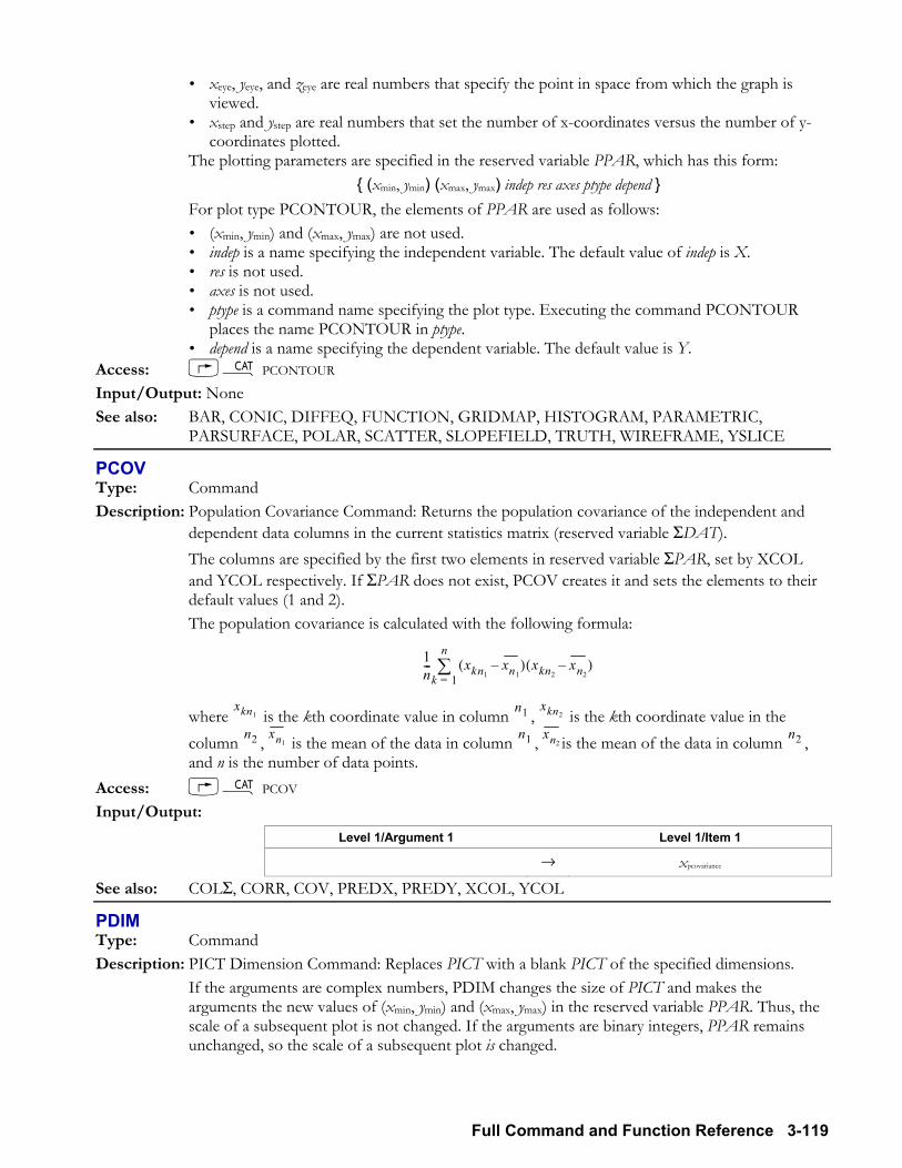
Full Command and Function Reference 3-119
xeye, yeye, and zeye are real numbers that specify the point in space from which the graph is viewed.
xstep and ystep are real numbers that set the number of x-coordinates versus the number of y-coordinates plotted.
The plotting parameters are specified in the reserved variable PPAR, which has this form: (xmin, ymin) (xmax, ymax) indep res axes ptype depend
For plot type PCONTOUR, the elements of PPAR are used as follows: (xmin, ymin) and (xmax, ymax) are not used. indep is a name specifying the independent variable. The default value of indep is X. res is not used. axes is not used. ptype is a command name specifying the plot type. Executing the command PCONTOUR
places the name PCONTOUR in ptype. depend is a name specifying the dependent variable. The default value is Y.
Access: µ PCONTOUR Input/Output: None See also: BAR, CONIC, DIFFEQ, FUNCTION, GRIDMAP, HISTOGRAM, PARAMETRIC,
PARSURFACE, POLAR, SCATTER, SLOPEFIELD, TRUTH, WIREFRAME, YSLICE
PCOV Type: Command Description: Population Covariance Command: Returns the population covariance of the independent and
dependent data columns in the current statistics matrix (reserved variable ΣDAT). The columns are specified by the first two elements in reserved variable ΣPAR, set by XCOL
and YCOL respectively. If ΣPAR does not exist, PCOV creates it and sets the elements to their default values (1 and 2).
The population covariance is calculated with the following formula:
1n---
xkn1xn1
( ) xkn2xn2
( )k 1=
n∑
where xkn1 is the kth coordinate value in column n1 ,
xkn2 is the kth coordinate value in the column n2 , xn1 is the mean of the data in column n1 , xn2 is the mean of the data in column n2 , and n is the number of data points.
Access: µ PCOV Input/Output:
Level 1/Argument 1 Level 1/Item 1 → xpcovariance
See also: COLΣ, CORR, COV, PREDX, PREDY, XCOL, YCOL
PDIM Type: Command Description: PICT Dimension Command: Replaces PICT with a blank PICT of the specified dimensions. If the arguments are complex numbers, PDIM changes the size of PICT and makes the
arguments the new values of (xmin, ymin) and (xmax, ymax) in the reserved variable PPAR. Thus, the scale of a subsequent plot is not changed. If the arguments are binary integers, PPAR remains unchanged, so the scale of a subsequent plot is changed.
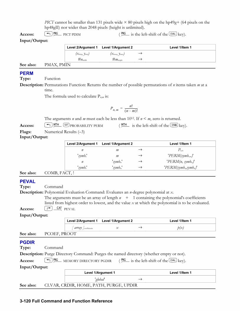
3-120 Full Command and Function Reference
PICT cannot be smaller than 131 pixels wide × 80 pixels high on the hp49g+ (64 pixels on the hp48gII) nor wider than 2048 pixels (height is unlimited).
Access: !°PICT PDIM ( °is the left-shift of the Nkey). Input/Output:
Level 2/Argument 1 Level 1/Argument 2 Level 1/Item 1
(xmin, ymin) (xmax, ymax) → #nwidth #mheight →
See also: PMAX, PMIN
PERM Type: Function Description: Permutations Function: Returns the number of possible permutations of n items taken m at a
time. The formula used to calculate Pn,m is:
Pn m,
n!n m( )!--------------------=
The arguments n and m must each be less than 1012. If n < m, zero is returned. Access: !´LPROBABILITY PERM ( ´ is the left-shift of the Pkey). Flags: Numerical Results (3) Input/Output:
Level 2/Argument 1 Level 1/Argument 2 Level 1/Item 1
n m → Pn,m 'symbn' m → 'PERM(symbn,m)'
n 'symbm' → 'PERM(n, symbm)' 'symbn' 'symbm' → 'PERM(symbn,symbm)'
See also: COMB, FACT, !
PEVAL Type: Command Description: Polynomial Evaluation Command: Evaluates an n-degree polynomial at x. The arguments must be an array of length n + 1 containing the polynomial's coefficients
listed from highest order to lowest, and the value x at which the polynomial is to be evaluated. Access: µ PEVAL Input/Output:
Level 2/Argument 1 Level 1/Argument 2 Level 1/Item 1
[ array ]coefficients x → p(x) See also: PCOEF, PROOT
PGDIR Type: Command Description: Purge Directory Command: Purges the named directory (whether empty or not). Access: !°MEMORY DIRECTORY PGDIR ( °is the left-shift of the Nkey). Input/Output:
Level 1/Argument 1 Level 1/Item 1
'global' → See also: CLVAR, CRDIR, HOME, PATH, PURGE, UPDIR
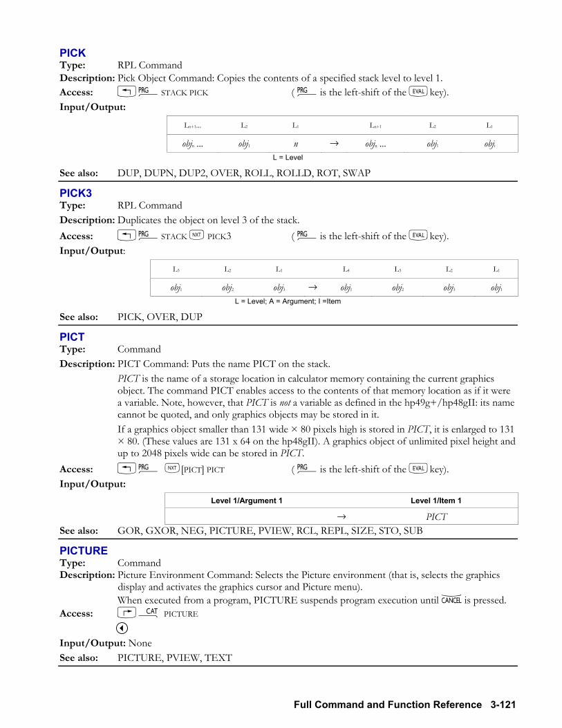
Full Command and Function Reference 3-121
PICK Type: RPL Command Description: Pick Object Command: Copies the contents of a specified stack level to level 1. Access: !°STACK PICK ( °is the left-shift of the Nkey). Input/Output:
Ln+1... L2 L1 Ln+1 L2 L1
objn ... obj1 n → objn ... obj1 obji L = Level
See also: DUP, DUPN, DUP2, OVER, ROLL, ROLLD, ROT, SWAP
PICK3 Type: RPL Command Description: Duplicates the object on level 3 of the stack. Access: !°STACK L PICK3 ( °is the left-shift of the Nkey). Input/Output:
L3 L2 L1 L4 L3 L2 L1
obj1 obj2 obj3 → obj1 obj2 obj3 obj1 L = Level; A = Argument; I =Item
See also: PICK, OVER, DUP
PICT Type: Command Description: PICT Command: Puts the name PICT on the stack. PICT is the name of a storage location in calculator memory containing the current graphics
object. The command PICT enables access to the contents of that memory location as if it were a variable. Note, however, that PICT is not a variable as defined in the hp49g+/hp48gII: its name cannot be quoted, and only graphics objects may be stored in it.
If a graphics object smaller than 131 wide × 80 pixels high is stored in PICT, it is enlarged to 131 × 80. (These values are 131 x 64 on the hp48gII). A graphics object of unlimited pixel height and up to 2048 pixels wide can be stored in PICT.
Access: !° L[PICT] PICT ( °is the left-shift of the Nkey). Input/Output:
Level 1/Argument 1 Level 1/Item 1
→ PICT See also: GOR, GXOR, NEG, PICTURE, PVIEW, RCL, REPL, SIZE, STO, SUB
PICTURE Type: Command Description: Picture Environment Command: Selects the Picture environment (that is, selects the graphics
display and activates the graphics cursor and Picture menu). When executed from a program, PICTURE suspends program execution until −is pressed. Access: µ PICTURE Input/Output: None See also: PICTURE, PVIEW, TEXT
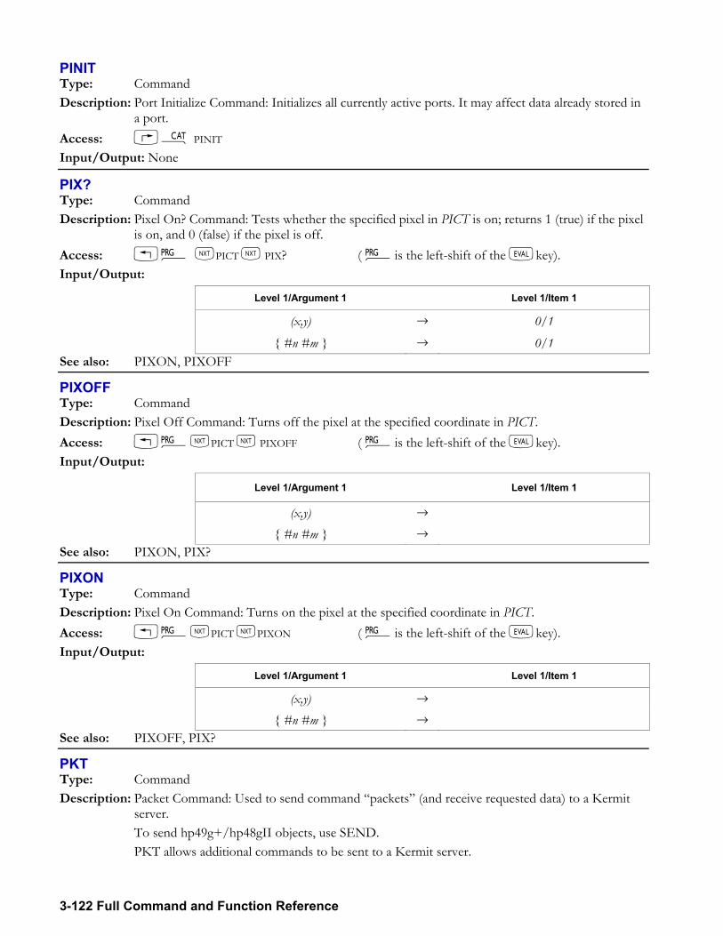
3-122 Full Command and Function Reference
PINIT Type: Command Description: Port Initialize Command: Initializes all currently active ports. It may affect data already stored in
a port. Access: µ PINIT Input/Output: None
PIX? Type: Command Description: Pixel On? Command: Tests whether the specified pixel in PICT is on; returns 1 (true) if the pixel
is on, and 0 (false) if the pixel is off. Access: !° LPICT L PIX? ( °is the left-shift of the Nkey). Input/Output:
Level 1/Argument 1 Level 1/Item 1
(x,y) → 0/1
#n #m → 0/1 See also: PIXON, PIXOFF
PIXOFF Type: Command Description: Pixel Off Command: Turns off the pixel at the specified coordinate in PICT. Access: !°LPICT L PIXOFF ( °is the left-shift of the Nkey). Input/Output:
Level 1/Argument 1 Level 1/Item 1
(x,y) → #n #m →
See also: PIXON, PIX?
PIXON Type: Command Description: Pixel On Command: Turns on the pixel at the specified coordinate in PICT. Access: !°LPICT LPIXON ( °is the left-shift of the Nkey). Input/Output:
Level 1/Argument 1 Level 1/Item 1
(x,y) → #n #m →
See also: PIXOFF, PIX?
PKT Type: Command Description: Packet Command: Used to send command packets (and receive requested data) to a Kermit
server. To send hp49g+/hp48gII objects, use SEND. PKT allows additional commands to be sent to a Kermit server.
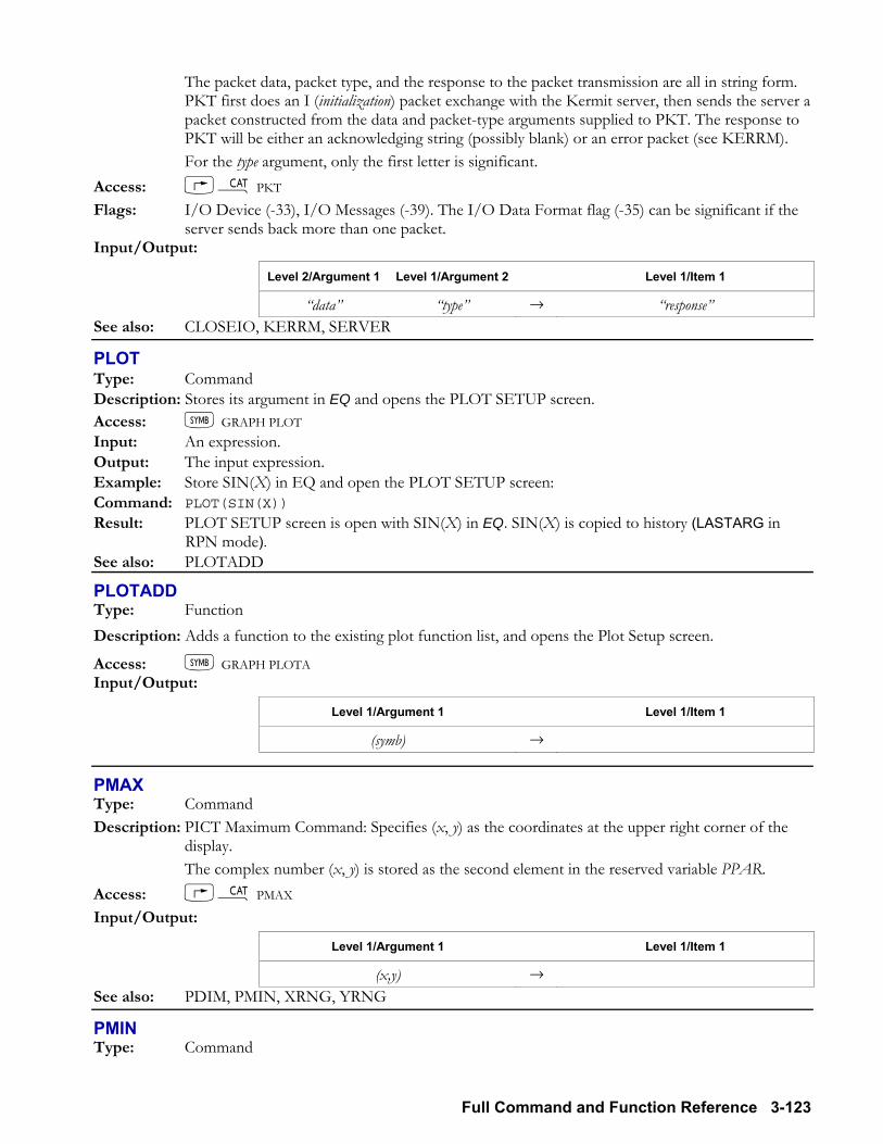
Full Command and Function Reference 3-123
The packet data, packet type, and the response to the packet transmission are all in string form. PKT first does an I (initialization) packet exchange with the Kermit server, then sends the server a packet constructed from the data and packet-type arguments supplied to PKT. The response to PKT will be either an acknowledging string (possibly blank) or an error packet (see KERRM).
For the type argument, only the first letter is significant. Access: µ PKT Flags: I/O Device (-33), I/O Messages (-39). The I/O Data Format flag (-35) can be significant if the
server sends back more than one packet. Input/Output:
Level 2/Argument 1 Level 1/Argument 2 Level 1/Item 1
data type → response See also: CLOSEIO, KERRM, SERVER
PLOT Type: Command Description: Stores its argument in EQ and opens the PLOT SETUP screen. Access: P GRAPH PLOT Input: An expression. Output: The input expression. Example: Store SIN(X) in EQ and open the PLOT SETUP screen: Command: PLOT(SIN(X))
Result: PLOT SETUP screen is open with SIN(X) in EQ. SIN(X) is copied to history (LASTARG in RPN mode).
See also: PLOTADD
PLOTADD Type: Function Description: Adds a function to the existing plot function list, and opens the Plot Setup screen.
Access: P GRAPH PLOTA Input/Output:
Level 1/Argument 1 Level 1/Item 1
(symb) →
PMAX Type: Command Description: PICT Maximum Command: Specifies (x, y) as the coordinates at the upper right corner of the
display. The complex number (x, y) is stored as the second element in the reserved variable PPAR. Access: µ PMAX Input/Output:
Level 1/Argument 1 Level 1/Item 1
(x,y) → See also: PDIM, PMIN, XRNG, YRNG
PMIN Type: Command
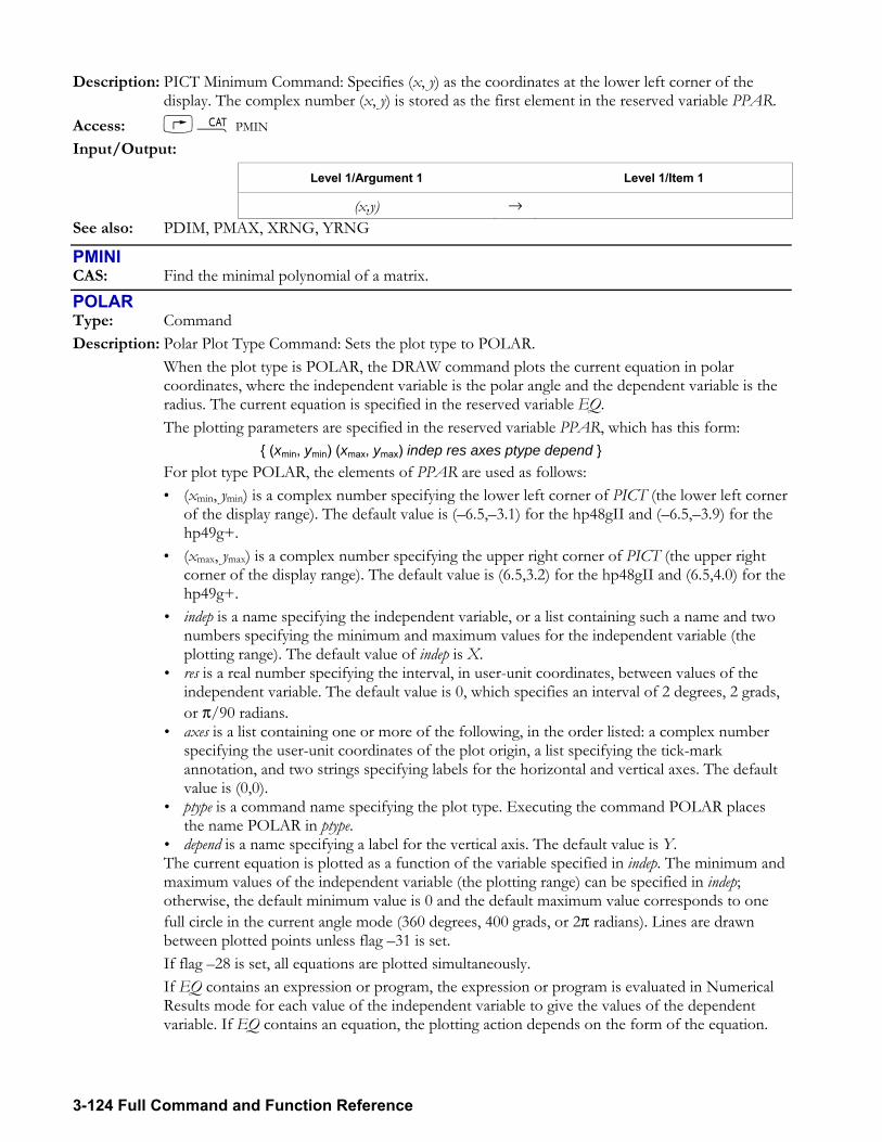
3-124 Full Command and Function Reference
Description: PICT Minimum Command: Specifies (x, y) as the coordinates at the lower left corner of the display. The complex number (x, y) is stored as the first element in the reserved variable PPAR.
Access: µ PMIN Input/Output:
Level 1/Argument 1 Level 1/Item 1
(x,y) → See also: PDIM, PMAX, XRNG, YRNG
PMINI CAS: Find the minimal polynomial of a matrix.
POLAR Type: Command Description: Polar Plot Type Command: Sets the plot type to POLAR. When the plot type is POLAR, the DRAW command plots the current equation in polar
coordinates, where the independent variable is the polar angle and the dependent variable is the radius. The current equation is specified in the reserved variable EQ.
The plotting parameters are specified in the reserved variable PPAR, which has this form: (xmin, ymin) (xmax, ymax) indep res axes ptype depend
For plot type POLAR, the elements of PPAR are used as follows: (xmin, ymin) is a complex number specifying the lower left corner of PICT (the lower left corner
of the display range). The default value is (6.5,3.1) for the hp48gII and (6.5,3.9) for the hp49g+.
(xmax, ymax) is a complex number specifying the upper right corner of PICT (the upper right corner of the display range). The default value is (6.5,3.2) for the hp48gII and (6.5,4.0) for the hp49g+.
indep is a name specifying the independent variable, or a list containing such a name and two numbers specifying the minimum and maximum values for the independent variable (the plotting range). The default value of indep is X.
res is a real number specifying the interval, in user-unit coordinates, between values of the independent variable. The default value is 0, which specifies an interval of 2 degrees, 2 grads, or π/90 radians.
axes is a list containing one or more of the following, in the order listed: a complex number specifying the user-unit coordinates of the plot origin, a list specifying the tick-mark annotation, and two strings specifying labels for the horizontal and vertical axes. The default value is (0,0).
ptype is a command name specifying the plot type. Executing the command POLAR places the name POLAR in ptype.
depend is a name specifying a label for the vertical axis. The default value is Y. The current equation is plotted as a function of the variable specified in indep. The minimum and
maximum values of the independent variable (the plotting range) can be specified in indep; otherwise, the default minimum value is 0 and the default maximum value corresponds to one full circle in the current angle mode (360 degrees, 400 grads, or 2π radians). Lines are drawn between plotted points unless flag 31 is set.
If flag 28 is set, all equations are plotted simultaneously. If EQ contains an expression or program, the expression or program is evaluated in Numerical
Results mode for each value of the independent variable to give the values of the dependent variable. If EQ contains an equation, the plotting action depends on the form of the equation.
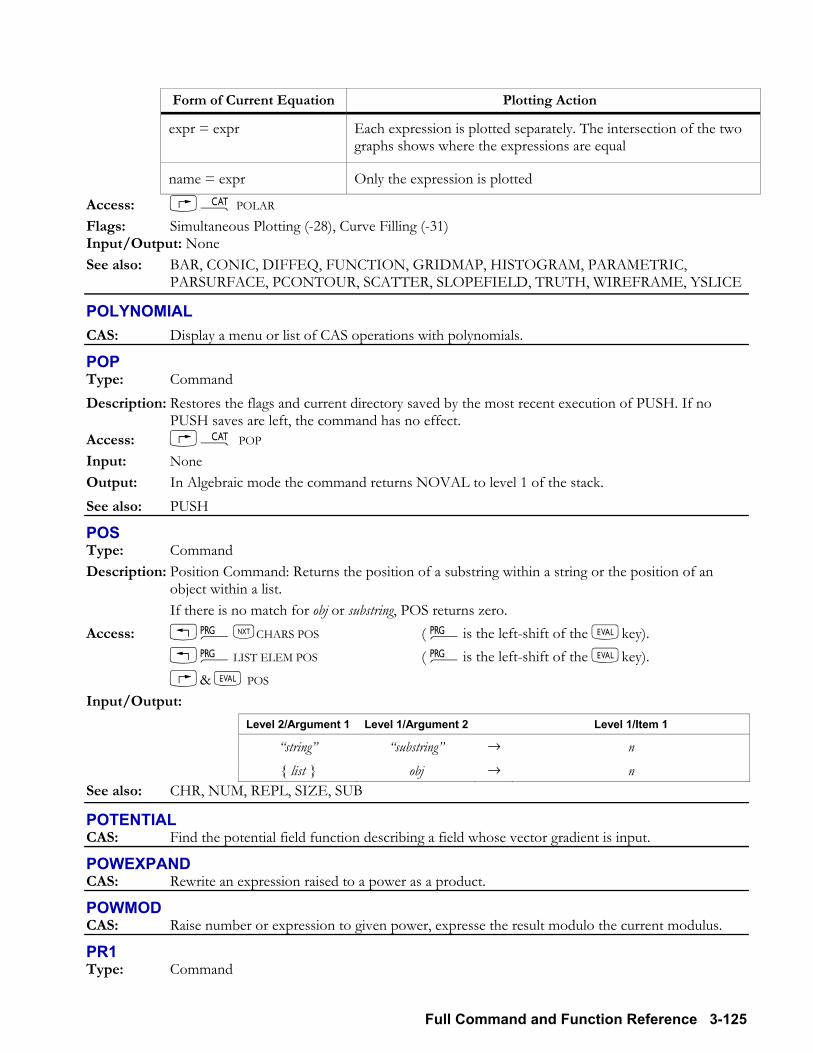
Full Command and Function Reference 3-125
Form of Current Equation Plotting Action
expr = expr Each expression is plotted separately. The intersection of the two graphs shows where the expressions are equal
name = expr Only the expression is plotted
Access: µ POLAR Flags: Simultaneous Plotting (-28), Curve Filling (-31) Input/Output: None See also: BAR, CONIC, DIFFEQ, FUNCTION, GRIDMAP, HISTOGRAM, PARAMETRIC,
PARSURFACE, PCONTOUR, SCATTER, SLOPEFIELD, TRUTH, WIREFRAME, YSLICE
POLYNOMIAL CAS: Display a menu or list of CAS operations with polynomials.
POP Type: Command Description: Restores the flags and current directory saved by the most recent execution of PUSH. If no
PUSH saves are left, the command has no effect. Access: µ POP Input: None Output: In Algebraic mode the command returns NOVAL to level 1 of the stack. See also: PUSH
POS Type: Command Description: Position Command: Returns the position of a substring within a string or the position of an
object within a list. If there is no match for obj or substring, POS returns zero. Access: !°LCHARS POS ( °is the left-shift of the Nkey). !°LIST ELEM POS ( °is the left-shift of the Nkey). @& N POS Input/Output:
Level 2/Argument 1 Level 1/Argument 2 Level 1/Item 1
string substring → n list obj → n
See also: CHR, NUM, REPL, SIZE, SUB
POTENTIAL CAS: Find the potential field function describing a field whose vector gradient is input.
POWEXPAND CAS: Rewrite an expression raised to a power as a product.
POWMOD CAS: Raise number or expression to given power, expresse the result modulo the current modulus.
PR1 Type: Command
3-126 Full Command and Function Reference
Description: Print Level 1 Command: Prints an object in multiline printer format. All objects except strings are printed with their identifying delimiters. Strings are printed without
the leading and trailing " delimiters. Multiline printer format is similar to multiline display format, with the following exceptions:
Strings and names that are more than 24 characters long are continued on the next printer line.
The real and imaginary parts of complex numbers are printed on separate lines if they don't fit on the same line.
Grobs are printed graphically. Arrays are printed with a numbered heading for each row and with a column number before
each element. For example, the 2 × 3 array
1 2 34 5 6
would be printed as follows: Array (2 3) Row 1 1] 1 2] 2 3] 3 Row 2 1] 4 2] 5 3] 6
Access: µ PR1 Flags: I/O Device (-33), Printing Device (-34), Double-spaced Printing (-37), Linefeed (-38). If flag -34
is set, flag -33 must be clear. Input/Output:
Level 1/Argument 1 Level 1/Item 1
object → object See also: CR, DELAY, OLDPRT, PRLCD, PRST, PRSTC, PRVAR
PREDV Type: Command Description: Predicted y-Value Command: Returns the predicted dependent-variable value ydependent, based on
the independent-variable value xindependent, the currently selected statistical model, and the current regression coefficients in the reserved variable ΣPAR.
PREDV is the same as PREDY. See PREDY. Access: µ PREDV Input/Output:
Level 1/Argument 1 Level 1/Item 1
xindependent → ydependent See also: PREDY
PREDX Type: Command
Full Command and Function Reference 3-127
Description: Predicted x-Value Command: Returns the predicted independent-variable value xindependent, based on the dependent-variable value ydependent, the currently selected statistical model, and the current regression coefficients in the reserved variable ΣPAR.
The value is predicted using the regression coefficients most recently computed with LR and stored in the reserved variable ΣPAR. For the linear statistical model, the equation used is this:
ydependent = (mxindependent) + b
where m is the slope (the third element in ΣPAR) and b is the intercept (the fourth element in ΣPAR).
For the other statistical models, the equations used by PREDX are listed in the LR entry. If PREDX is executed without having previously generated regression coefficients in ΣPAR, a
default value of zero is used for both regression coefficients, and an error results. Access: µ PREDX Input/Output:
Level 1/Argument 1 Level 1/Item 1
ydependent → xindependent See also: COLΣ, CORR, COV, EXPFIT, ΣLINE, LINFIT, LOGFIT, LR, PREDY, PWRFIT, XCOL,
YCOL
PREDY Type: Command Description: Predicted y-Value Command: Returns the predicted dependent-variable value ydependent, based on
the independent-variable value xindependent, the currently selected statistical model, and the current regression coefficients in the reserved variable ΣPAR.
The value is predicted using the regression coefficients most recently computed with LR and stored in the reserved variable ΣPAR. For the linear statistical model, the equation used is this:
ydependent = (mxindependent) + b
where m is the slope (the third element in ΣPAR) and b is the intercept (the fourth element in ΣPAR).
For the other statistical models, the equations used by PREDY are listed in the LR entry. If PREDY is executed without having previously generated regression coefficients in ΣPAR, a
default value of zero is used for both regression coefficientsin this case PREDY will return 0 for statistical models LINFIT and LOGFIT, and error for statistical models EXPFIT and PWRFIT.
Access: µ PREDY Input/Output:
Level 1/Argument 1 Level 1/Item 1
xindependent → ydependent See also: COLΣ, CORR, COV, EXPFIT, ΣLINE, LINFIT, LOGFIT, LR, PREDX, PWRFIT, XCOL,
YCOL
PREVAL CAS: Return difference between values of a function at two specified values of the current variable.
PREVPRIME CAS: Given an integer, find the closest prime number smaller than the integer.
3-128 Full Command and Function Reference
PRLCD Type: Command Description: Print LCD Command: Prints a pixel-by-pixel image of the current display (excluding the
annunciators). The width of the printed image of characters in the display is narrower using PRLCD than using
a print command such as PR1. The difference results from the spacing between characters. On the display there is a single blank column between characters, and PRLCD prints this spacing. Print commands such as PR1 print two blank columns between adjacent characters.
Access: µ PRLCD Flags: I/O Device (-33), Printing Device (-34), Double-spaced Printing (-37), Linefeed (-38). Flag -38
must be clear. If flag -34 is set, flag -33 must be clear. Input/Output: None See also: CR, DELAY, OLDPRT, PRST, PRSTC, PRVAR, PR1
PROMPT Type: Command Description: Prompt Command: Displays the contents of prompt in the status area, and halts program
execution. Access: !°LIN LPROMPT ( °is the left-shift of the Nkey). Input/Output:
Level 1/Argument 1 Level 1/Item 1
prompt →
See also: CONT, DISP, FREEZE, HALT, INFORM, INPUT, MSGBOX
PROMPTSTO Type: Command Description: Prompt Command: Creates a variable with the name supplied as an argument, prompts for a
value, and stores the value you enter in the variable. Access: µPROMPTSTO Input/Output:
Level 1/Argument 1 Level 1/Item 1
global →
See also: PROMPT, STO
PROOT Type: Command Description: Polynomial Roots Command: Returns all roots of an n-degree polynomial having real or complex
coefficients. For an nth-order polynomial, the argument must be a real or complex array of length n + 1
containing the coefficients listed from highest order to lowest. The result is a real or complex vector of length n containing the computed roots.
PROOT interprets leading coefficients of zero in a limiting sense. As a leading coefficient approaches zero, a root of the polynomial approaches infinity: therefore, if flag 22 is clear (the default), PROOT reports an Infinite Result error if a leading coefficient is zero. If flag 22 is set, PROOT returns a root of (MAXREAL,0) for each leading zero in an array containing real coefficients, and a root of (MAXREAL,MAXREAL) for each leading zero in an array containing complex coefficients.
Access: !ÞPOLYNOMIAL LLPROOT (Þis the left-shift of the 1key).
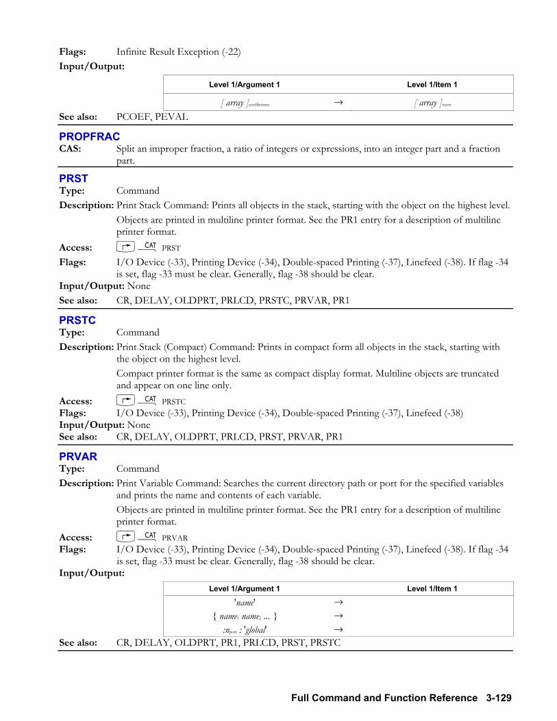
Full Command and Function Reference 3-129
Flags: Infinite Result Exception (-22) Input/Output:
Level 1/Argument 1 Level 1/Item 1
[ array ]coefficients → [ array ]roots See also: PCOEF, PEVAL
PROPFRAC CAS: Split an improper fraction, a ratio of integers or expressions, into an integer part and a fraction
part.
PRST Type: Command Description: Print Stack Command: Prints all objects in the stack, starting with the object on the highest level. Objects are printed in multiline printer format. See the PR1 entry for a description of multiline
printer format. Access: µ PRST Flags: I/O Device (-33), Printing Device (-34), Double-spaced Printing (-37), Linefeed (-38). If flag -34
is set, flag -33 must be clear. Generally, flag -38 should be clear. Input/Output: None See also: CR, DELAY, OLDPRT, PRLCD, PRSTC, PRVAR, PR1
PRSTC Type: Command Description: Print Stack (Compact) Command: Prints in compact form all objects in the stack, starting with
the object on the highest level. Compact printer format is the same as compact display format. Multiline objects are truncated
and appear on one line only. Access: µ PRSTC Flags: I/O Device (-33), Printing Device (-34), Double-spaced Printing (-37), Linefeed (-38) Input/Output: None See also: CR, DELAY, OLDPRT, PRLCD, PRST, PRVAR, PR1
PRVAR Type: Command Description: Print Variable Command: Searches the current directory path or port for the specified variables
and prints the name and contents of each variable. Objects are printed in multiline printer format. See the PR1 entry for a description of multiline
printer format. Access: µ PRVAR Flags: I/O Device (-33), Printing Device (-34), Double-spaced Printing (-37), Linefeed (-38). If flag -34
is set, flag -33 must be clear. Generally, flag -38 should be clear. Input/Output:
Level 1/Argument 1 Level 1/Item 1
'name' → name1 name2 ... →
:nport : 'global' → See also: CR, DELAY, OLDPRT, PR1, PRLCD, PRST, PRSTC
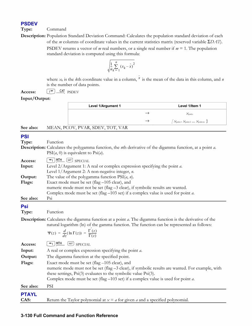
3-130 Full Command and Function Reference
PSDEV Type: Command Description: Population Standard Deviation Command: Calculates the population standard deviation of each
of the m columns of coordinate values in the current statistics matrix (reserved variable ΣDAT). PSDEV returns a vector of m real numbers, or a single real number if m = 1. The population
standard deviation is computed using this formula:
1n---
xk x( )2
k 1=
n∑
where xk is the kth coordinate value in a column, x is the mean of the data in this column, and n
is the number of data points. Access: µ PSDEV Input/Output:
Level 1/Argument 1 Level 1/Item 1
→ xpsdev
→ [ xpsdev1 xpsdev2 ... xpsdevm See also: MEAN, PCOV, PVAR, SDEV, TOT, VAR
PSI Type: Function Description: Calculates the polygamma function, the nth derivative of the digamma function, at a point a.
PSI(a, 0) is equivalent to Psi(a).
Access: !´L SPECIAL Input: Level 2/Argument 1: A real or complex expression specifying the point a. Level 1/Argument 2: A non-negative integer, n. Output: The value of the polygamma function PSI(a, n). Flags: Exact mode must be set (flag 105 clear), and
numeric mode must not be set (flag 3 clear), if symbolic results are wanted. Complex mode must be set (flag 103 set) if a complex value is used for point a.
See also: Psi
Psi Type: Function Description: Calculates the digamma function at a point a. The digamma function is the derivative of the
natural logarithm (ln) of the gamma function. The function can be represented as follows:
Ψ z( ) ddz----- Γ z( )ln( ) Γ′ z( )
Γ z( )------------= =
Access: !´ L SPECIAL Input: A real or complex expression specifying the point a. Output: The digamma function at the specified point. Flags: Exact mode must be set (flag 105 clear), and
numeric mode must not be set (flag 3 clear), if symbolic results are wanted. For example, with these settings, Psi(3) evaluates to the symbolic value Psi(3). Complex mode must be set (flag 103 set) if a complex value is used for point a.
See also: PSI
PTAYL CAS: Return the Taylor polynomial at x = a for given a and a specified polynomial.
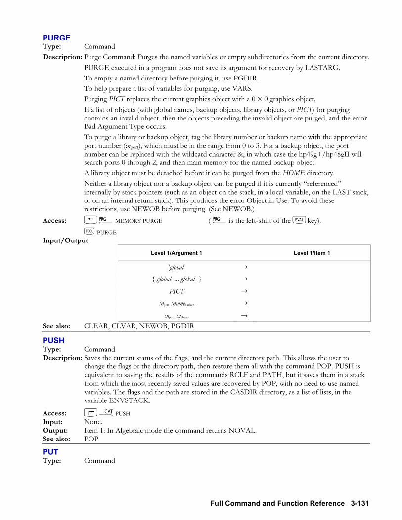
Full Command and Function Reference 3-131
PURGE Type: Command Description: Purge Command: Purges the named variables or empty subdirectories from the current directory. PURGE executed in a program does not save its argument for recovery by LASTARG. To empty a named directory before purging it, use PGDIR. To help prepare a list of variables for purging, use VARS. Purging PICT replaces the current graphics object with a 0 × 0 graphics object. If a list of objects (with global names, backup objects, library objects, or PICT) for purging
contains an invalid object, then the objects preceding the invalid object are purged, and the error Bad Argument Type occurs.
To purge a library or backup object, tag the library number or backup name with the appropriate port number (:nport), which must be in the range from 0 to 3. For a backup object, the port number can be replaced with the wildcard character &, in which case the hp49g+/hp48gII will search ports 0 through 2, and then main memory for the named backup object.
A library object must be detached before it can be purged from the HOME directory. Neither a library object nor a backup object can be purged if it is currently referenced
internally by stack pointers (such as an object on the stack, in a local variable, on the LAST stack, or on an internal return stack). This produces the error Object in Use. To avoid these restrictions, use NEWOB before purging. (See NEWOB.)
Access: !°MEMORY PURGE ( °is the left-shift of the Nkey). I PURGE Input/Output:
Level 1/Argument 1 Level 1/Item 1
'global' → global1 ... globaln →
PICT → :nport :namebackup →
:nport :nlibrary → See also: CLEAR, CLVAR, NEWOB, PGDIR
PUSH Type: Command Description: Saves the current status of the flags, and the current directory path. This allows the user to
change the flags or the directory path, then restore them all with the command POP. PUSH is equivalent to saving the results of the commands RCLF and PATH, but it saves them in a stack from which the most recently saved values are recovered by POP, with no need to use named variables. The flags and the path are stored in the CASDIR directory, as a list of lists, in the variable ENVSTACK.
Access: µPUSH Input: None. Output: Item 1: In Algebraic mode the command returns NOVAL. See also: POP
PUT Type: Command

3-132 Full Command and Function Reference
Description: Put Element Command: Replaces the object at a specified position (second input) in a specified array or list (first input) with a specifed object (third input). If the array or list is unnamed, returns the new array or list.
For matrices, nposition counts in row order. Access: !°LIST ELEMENTS PUT ( °is the left-shift of the Nkey). Input/Output:
Level 3/Argument 1 Level 2/Argument 2 Level 1/Argument 3 Level 1/Item 1
[[ matrix ]]1 nposition zput → [[ matrix ]]2 [[ matrix ]]1 nrow mcol zput → [[ matrix ]]2
'namematrix' nposition zput →
'namematrix' nrow mcol zput → [ vector ]1 nposition zput → [ vector ]2 [ vector ]1 nposition zput → [ vector ]2 'namevector' nposition zput → 'namevector' nposition zput → list 1 nposition objput → list 2 list 1 nposition objput → list 2 'namelist' nposition objput → 'namelist' nposition objput →
See also: GET, GETI, PUTI
PUTI Type: Command Description: Put and Increment Index Command: Replaces the object at a specified position (second input) in
a specified array or list (first input) with a specifed object (third input), returning a new array or list together with the next position in the array or list.
For matrices, the position is incremented in row order. Unlike PUT, PUTI returns a named array or list. This enables a subsequent execution of PUTI at
the next position of a named array or list. Access: !°LIST ELEMENTS PUTI ( °is the left-shift of the Nkey). Flags: Index Wrap Inidicator (-64)
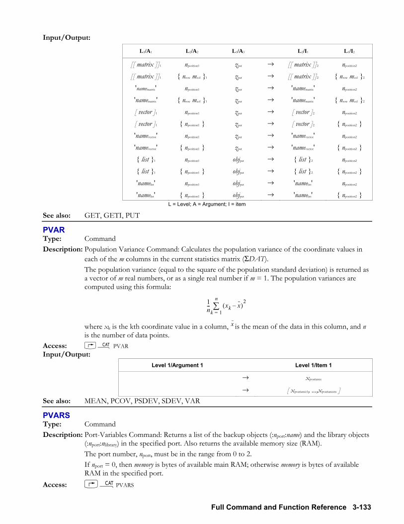
Full Command and Function Reference 3-133
Input/Output:
L3/A1 L2/A2 L1/A3 L2/I1 L1/I2
[[ matrix ]]1 nposition1 zput → [[ matrix ]]2 nposition2 [[ matrix ]]1 nrow mcol 1 zput → [[ matrix ]]2 nrow mcol 2
'namematrix' nposition1 zput → 'namematrix' nposition2 'namematrix' nrow mcol 1 zput → 'namematrix' nrow mcol 2 [ vector ]1 nposition1 zput → [ vector ]2 nposition2 [ vector ]1 nposition1 zput → [ vector ]2 nposition2 'namevector' nposition1 zput → 'namevector' nposition2 'namevector' nposition1 zput → 'namevector' nposition2 list 1 nposition1 objput → list 2 nposition2 list 1 nposition1 objput → list 2 nposition2 'namelist' nposition1 objput → 'namelist' nposition2 'namelist' nposition1 objput → 'namelist' nposition2
L = Level; A = Argument; I = item
See also: GET, GETI, PUT
PVAR Type: Command Description: Population Variance Command: Calculates the population variance of the coordinate values in
each of the m columns in the current statistics matrix (ΣDAT). The population variance (equal to the square of the population standard deviation) is returned as
a vector of m real numbers, or as a single real number if m = 1. The population variances are computed using this formula:
1n---
xk x( )2
k 1=
n∑
where xk is the kth coordinate value in a column, x is the mean of the data in this column, and n
is the number of data points. Access: µ PVAR Input/Output:
Level 1/Argument 1 Level 1/Item 1
→ xpvariance
→ [ xpvariance1, ...,xpvariancem ] See also: MEAN, PCOV, PSDEV, SDEV, VAR
PVARS Type: Command Description: Port-Variables Command: Returns a list of the backup objects (:nport:name) and the library objects
(:nport:nlibrary) in the specified port. Also returns the available memory size (RAM). The port number, nport, must be in the range from 0 to 2. If nport = 0, then memory is bytes of available main RAM; otherwise memory is bytes of available
RAM in the specified port. Access: µPVARS
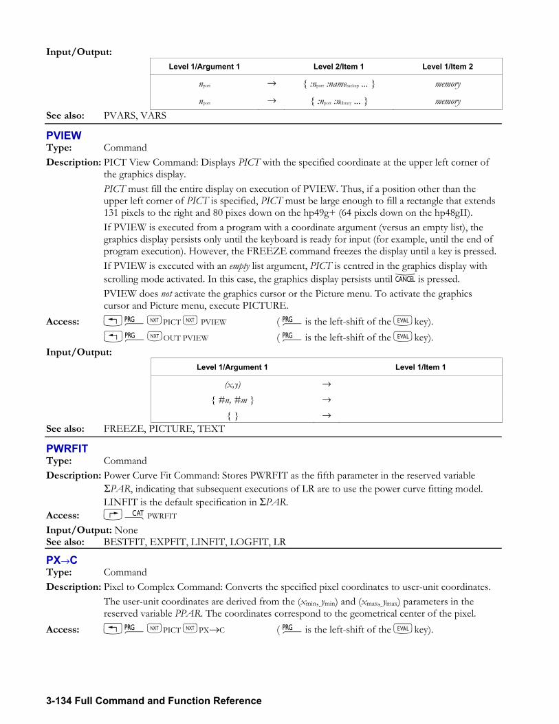
3-134 Full Command and Function Reference
Input/Output: Level 1/Argument 1 Level 2/Item 1 Level 1/Item 2
nport → :nport :namebackup ... memory
nport → :nport :nlibrary ... memory See also: PVARS, VARS
PVIEW Type: Command Description: PICT View Command: Displays PICT with the specified coordinate at the upper left corner of
the graphics display. PICT must fill the entire display on execution of PVIEW. Thus, if a position other than the
upper left corner of PICT is specified, PICT must be large enough to fill a rectangle that extends 131 pixels to the right and 80 pixes down on the hp49g+ (64 pixels down on the hp48gII).
If PVIEW is executed from a program with a coordinate argument (versus an empty list), the graphics display persists only until the keyboard is ready for input (for example, until the end of program execution). However, the FREEZE command freezes the display until a key is pressed.
If PVIEW is executed with an empty list argument, PICT is centred in the graphics display with scrolling mode activated. In this case, the graphics display persists until −is pressed.
PVIEW does not activate the graphics cursor or the Picture menu. To activate the graphics cursor and Picture menu, execute PICTURE.
Access: !°LPICT L PVIEW ( °is the left-shift of the Nkey). !°LOUT PVIEW ( °is the left-shift of the Nkey). Input/Output:
Level 1/Argument 1 Level 1/Item 1
(x,y) → #n, #m →
→ See also: FREEZE, PICTURE, TEXT
PWRFIT Type: Command Description: Power Curve Fit Command: Stores PWRFIT as the fifth parameter in the reserved variable
ΣPAR, indicating that subsequent executions of LR are to use the power curve fitting model. LINFIT is the default specification in ΣPAR. Access: µPWRFIT Input/Output: None See also: BESTFIT, EXPFIT, LINFIT, LOGFIT, LR
PX→C Type: Command Description: Pixel to Complex Command: Converts the specified pixel coordinates to user-unit coordinates. The user-unit coordinates are derived from the (xmin, ymin) and (xmax, ymax) parameters in the
reserved variable PPAR. The coordinates correspond to the geometrical center of the pixel. Access: !°LPICT LPX→C ( °is the left-shift of the Nkey).
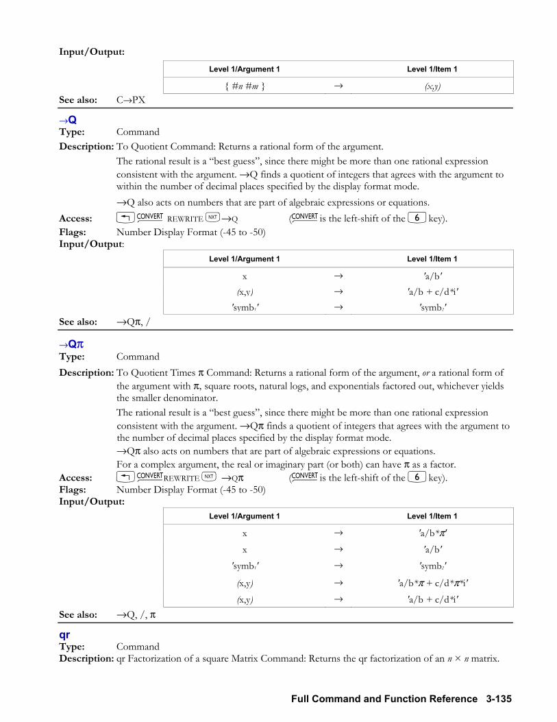
Full Command and Function Reference 3-135
Input/Output: Level 1/Argument 1 Level 1/Item 1
#n #m → (x,y) See also: C→PX
→Q Type: Command Description: To Quotient Command: Returns a rational form of the argument. The rational result is a best guess, since there might be more than one rational expression
consistent with the argument. →Q finds a quotient of integers that agrees with the argument to within the number of decimal places specified by the display format mode.
→Q also acts on numbers that are part of algebraic expressions or equations. Access: Ú REWRITE L→Q (Ú is the left-shift of the 6key). Flags: Number Display Format (-45 to -50) Input/Output:
Level 1/Argument 1 Level 1/Item 1
x → 'a/b' (x,y) → 'a/b + c/d*i'
'symb1' → 'symb2' See also: →Qπ, /
→Qπ Type: Command Description: To Quotient Times π Command: Returns a rational form of the argument, or a rational form of
the argument with π, square roots, natural logs, and exponentials factored out, whichever yields the smaller denominator.
The rational result is a best guess, since there might be more than one rational expression consistent with the argument. →Qπ finds a quotient of integers that agrees with the argument to the number of decimal places specified by the display format mode.
→Qπ also acts on numbers that are part of algebraic expressions or equations. For a complex argument, the real or imaginary part (or both) can have π as a factor. Access: Ú REWRITE L →Qπ (Ú is the left-shift of the 6key). Flags: Number Display Format (-45 to -50) Input/Output:
Level 1/Argument 1 Level 1/Item 1
x → 'a/b*π' x → 'a/b'
'symb1' → 'symb2'
(x,y) → 'a/b*π + c/d*π*i' (x,y) → 'a/b + c/d*i'
See also: →Q, /, π
qr Type: Command Description: qr Factorization of a square Matrix Command: Returns the qr factorization of an n × n matrix.
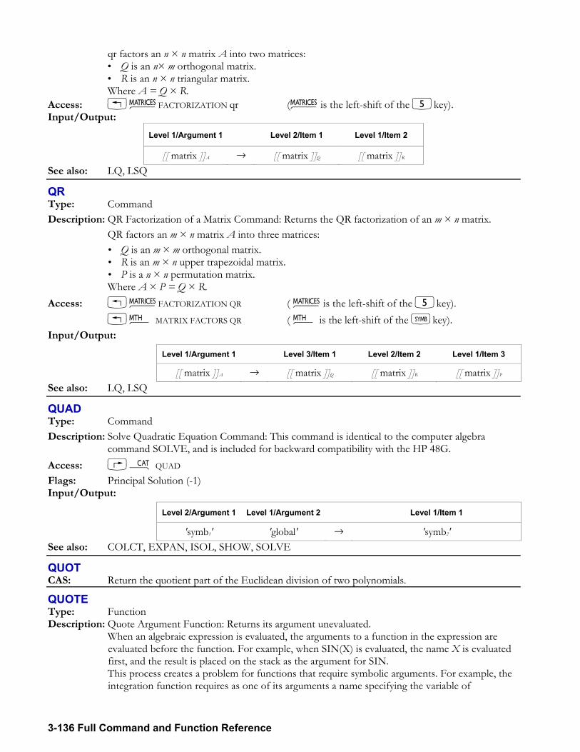
3-136 Full Command and Function Reference
qr factors an n × n matrix A into two matrices: Q is an n× m orthogonal matrix. R is an n × n triangular matrix.
Where A = Q × R. Access: !Ø FACTORIZATION qr (Ø is the left-shift of the 5key). Input/Output:
Level 1/Argument 1 Level 2/Item 1 Level 1/Item 2
[[ matrix ]]A → [[ matrix ]]Q [[ matrix ]]R See also: LQ, LSQ
QR Type: Command Description: QR Factorization of a Matrix Command: Returns the QR factorization of an m × n matrix. QR factors an m × n matrix A into three matrices:
Q is an m × m orthogonal matrix. R is an m × n upper trapezoidal matrix. P is a n × n permutation matrix.
Where A × P = Q × R. Access: !Ø FACTORIZATION QR ( Ø is the left-shift of the 5key). !´ MATRIX FACTORS QR ( ´ is the left-shift of the Pkey). Input/Output:
Level 1/Argument 1 Level 3/Item 1 Level 2/Item 2 Level 1/Item 3
[[ matrix ]]A → [[ matrix ]]Q [[ matrix ]]R [[ matrix ]]P See also: LQ, LSQ
QUAD Type: Command Description: Solve Quadratic Equation Command: This command is identical to the computer algebra
command SOLVE, and is included for backward compatibility with the HP 48G. Access: µ QUAD Flags: Principal Solution (-1) Input/Output:
Level 2/Argument 1 Level 1/Argument 2 Level 1/Item 1
'symb1' 'global' → 'symb2' See also: COLCT, EXPAN, ISOL, SHOW, SOLVE
QUOT CAS: Return the quotient part of the Euclidean division of two polynomials.
QUOTE Type: Function Description: Quote Argument Function: Returns its argument unevaluated. When an algebraic expression is evaluated, the arguments to a function in the expression are
evaluated before the function. For example, when SIN(X) is evaluated, the name X is evaluated first, and the result is placed on the stack as the argument for SIN.
This process creates a problem for functions that require symbolic arguments. For example, the integration function requires as one of its arguments a name specifying the variable of
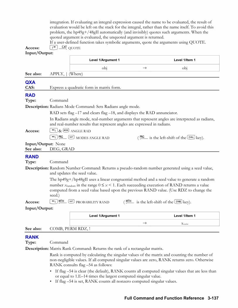
Full Command and Function Reference 3-137
integration. If evaluating an integral expression caused the name to be evaluated, the result of evaluation would be left on the stack for the integral, rather than the name itself. To avoid this problem, the hp49g+/48gII automatically (and invisibly) quotes such arguments. When the quoted argument is evaluated, the unquoted argument is returned.
If a user-defined function takes symbolic arguments, quote the arguments using QUOTE. Access: µQUOTE Input/Output:
Level 1/Argument 1 Level 1/Item 1
obj → obj See also: APPLY, | (Where)
QXA CAS: Express a quadratic form in matrix form.
RAD Type: Command Description: Radians Mode Command: Sets Radians angle mode. RAD sets flag 17 and clears flag 18, and displays the RAD annunciator. In Radians angle mode, real-number arguments that represent angles are interpreted as radians,
and real-number results that represent angles are expressed in radians. Access: & H ANGLE RAD °L MODES ANGLE RAD ( °is the left-shift of the Nkey). Input/Output: None See also: DEG, GRAD
RAND Type: Command Description: Random Number Command: Returns a pseudo-random number generated using a seed value,
and updates the seed value. The hp49g+/hp48gII uses a linear congruential method and a seed value to generate a random
number xrandom in the range 0 ≤ x < 1. Each succeeding execution of RAND returns a value computed from a seed value based upon the previous RAND value. (Use RDZ to change the seed.)
Access: !´L PROBABILITY RAND ( ´ is the left-shift of the Pkey). Input/Output:
Level 1/Argument 1 Level 1/Item 1
→ xrandom See also: COMB, PERM RDZ, !
RANK Type: Command Description: Matrix Rank Command: Returns the rank of a rectangular matrix. Rank is computed by calculating the singular values of the matrix and counting the number of
non-negligible values. If all computed singular values are zero, RANK returns zero. Otherwise RANK consults flag 54 as follows: If flag 54 is clear (the default), RANK counts all computed singular values that are less than
or equal to 1.E14 times the largest computed singular value. If flag 54 is set, RANK counts all nonzero computed singular values.
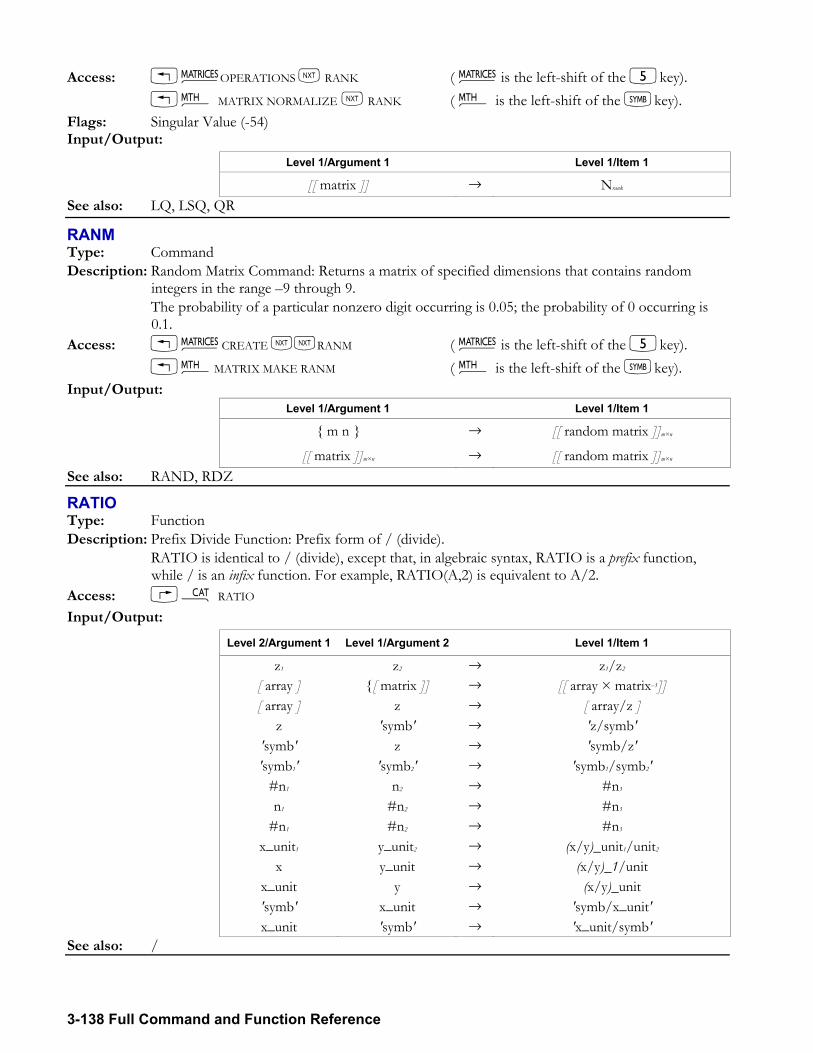
3-138 Full Command and Function Reference
Access: !Ø OPERATIONS L RANK ( Ø is the left-shift of the 5key). !´ MATRIX NORMALIZE L RANK ( ´ is the left-shift of the Pkey). Flags: Singular Value (-54) Input/Output:
Level 1/Argument 1 Level 1/Item 1
[[ matrix ]] → Nrank See also: LQ, LSQ, QR
RANM Type: Command Description: Random Matrix Command: Returns a matrix of specified dimensions that contains random
integers in the range 9 through 9. The probability of a particular nonzero digit occurring is 0.05; the probability of 0 occurring is
0.1. Access: !Ø CREATE LLRANM ( Ø is the left-shift of the 5key). !´MATRIX MAKE RANM ( ´ is the left-shift of the Pkey). Input/Output:
Level 1/Argument 1 Level 1/Item 1
m n → [[ random matrix ]]m×n
[[ matrix ]]m×n → [[ random matrix ]]m×n See also: RAND, RDZ
RATIO Type: Function Description: Prefix Divide Function: Prefix form of / (divide). RATIO is identical to / (divide), except that, in algebraic syntax, RATIO is a prefix function,
while / is an infix function. For example, RATIO(A,2) is equivalent to A/2. Access: µ RATIO Input/Output:
Level 2/Argument 1 Level 1/Argument 2 Level 1/Item 1
z1 z2 → z1/z2 [ array ] [ matrix ]] → [[ array × matrix1]] [ array ] z → [ array/z ]
z 'symb' → 'z/symb' 'symb' z → 'symb/z' 'symb1' 'symb2' → 'symb1/symb2'
#n1 n2 → #n3 n1 #n2 → #n3
#n1 #n2 → #n3 x_unit1 y_unit2 → (x/y)_unit1/unit2
x y_unit → (x/y)_1/unit x_unit y → (x/y)_unit 'symb' x_unit → 'symb/x_unit' x_unit 'symb' → 'x_unit/symb'
See also: /
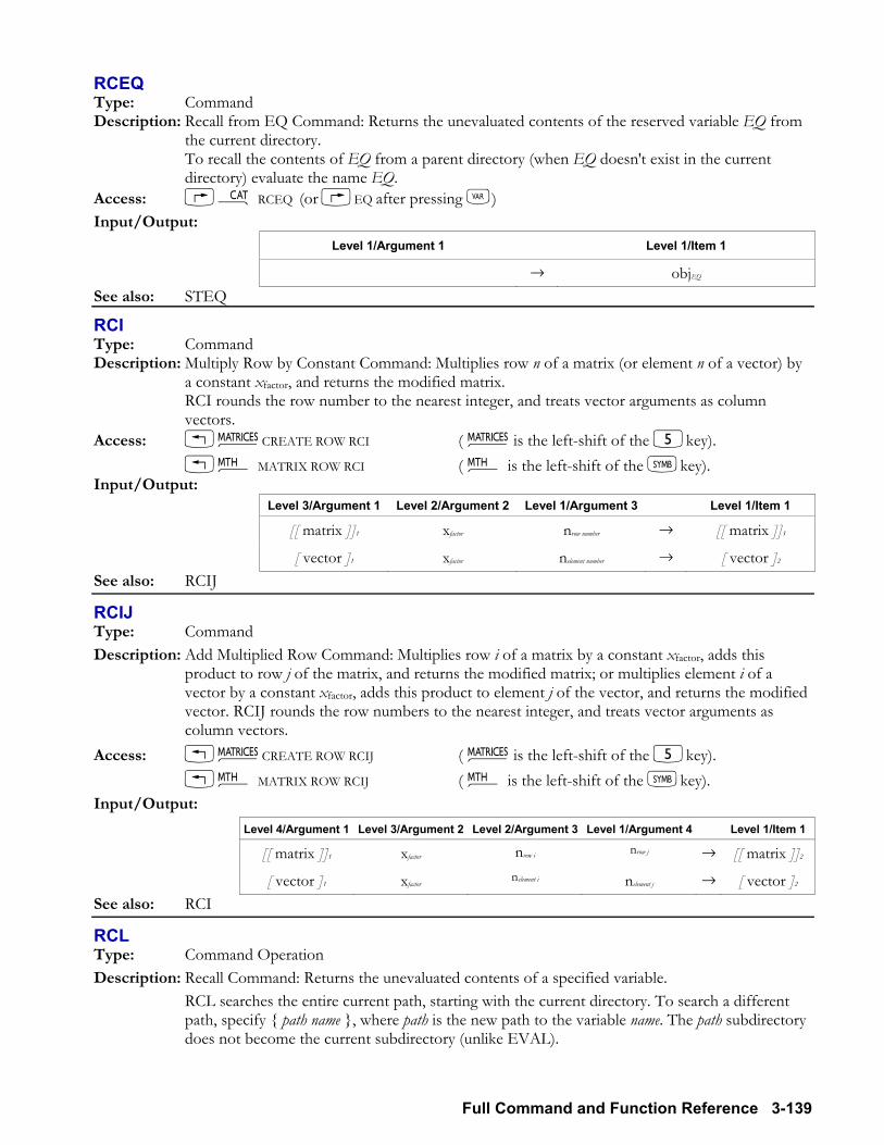
Full Command and Function Reference 3-139
RCEQ Type: Command Description: Recall from EQ Command: Returns the unevaluated contents of the reserved variable EQ from
the current directory. To recall the contents of EQ from a parent directory (when EQ doesn't exist in the current
directory) evaluate the name EQ. Access: µ RCEQ (or EQ after pressing J) Input/Output:
Level 1/Argument 1 Level 1/Item 1
→ objEQ See also: STEQ
RCI Type: Command Description: Multiply Row by Constant Command: Multiplies row n of a matrix (or element n of a vector) by
a constant xfactor, and returns the modified matrix. RCI rounds the row number to the nearest integer, and treats vector arguments as column
vectors. Access: !Ø CREATE ROW RCI ( Ø is the left-shift of the 5key). !´ MATRIX ROW RCI ( ´ is the left-shift of the Pkey). Input/Output:
Level 3/Argument 1 Level 2/Argument 2 Level 1/Argument 3 Level 1/Item 1
[[ matrix ]]1 xfactor nrow number → [[ matrix ]]3
[ vector ]1 xfactor nelement number → [ vector ]2 See also: RCIJ
RCIJ Type: Command Description: Add Multiplied Row Command: Multiplies row i of a matrix by a constant xfactor, adds this
product to row j of the matrix, and returns the modified matrix; or multiplies element i of a vector by a constant xfactor, adds this product to element j of the vector, and returns the modified vector. RCIJ rounds the row numbers to the nearest integer, and treats vector arguments as column vectors.
Access: !Ø CREATE ROW RCIJ ( Ø is the left-shift of the 5key). !´ MATRIX ROW RCIJ ( ´ is the left-shift of the Pkey). Input/Output:
Level 4/Argument 1 Level 3/Argument 2 Level 2/Argument 3 Level 1/Argument 4 Level 1/Item 1
[[ matrix ]]1 xfactor nrow i nrow j → [[ matrix ]]2
[ vector ]1 xfactor nelement i nelement j → [ vector ]2 See also: RCI
RCL Type: Command Operation Description: Recall Command: Returns the unevaluated contents of a specified variable. RCL searches the entire current path, starting with the current directory. To search a different
path, specify path name , where path is the new path to the variable name. The path subdirectory does not become the current subdirectory (unlike EVAL).
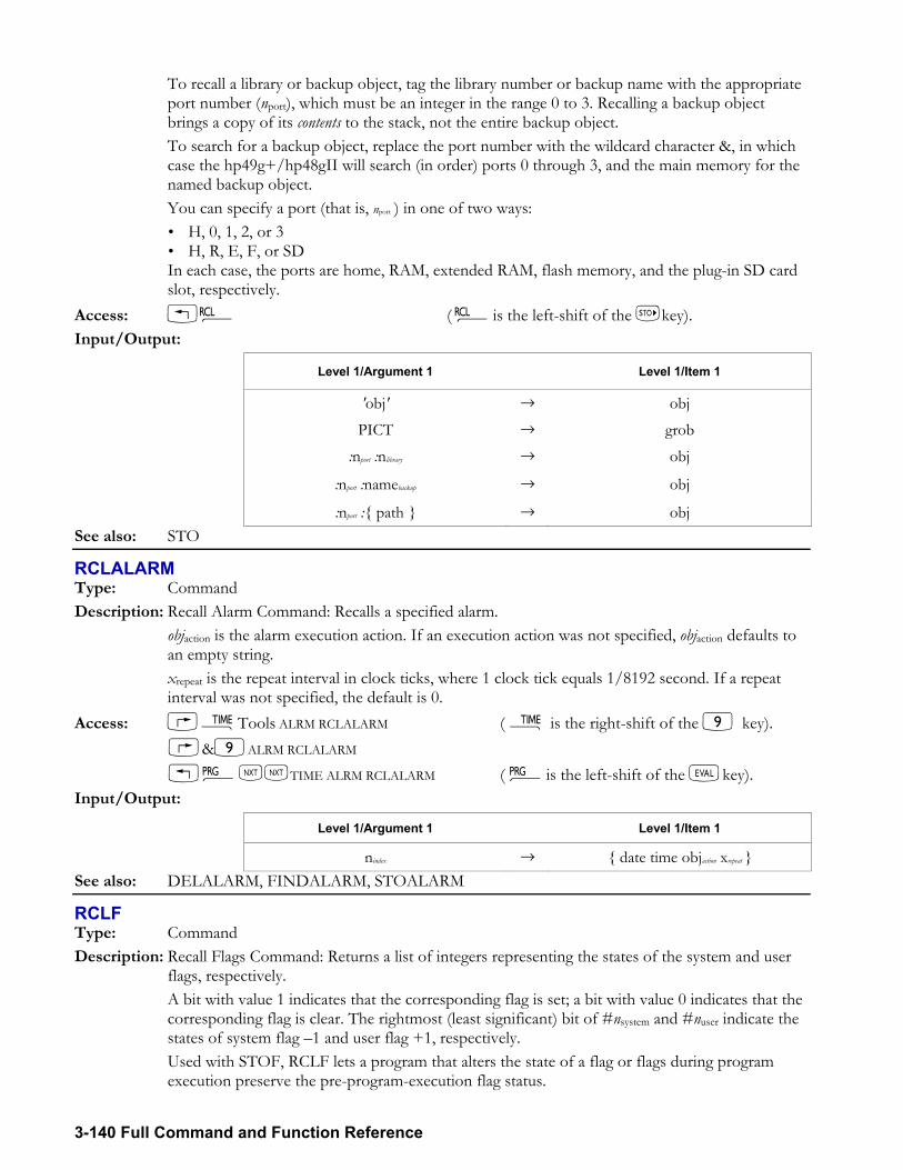
3-140 Full Command and Function Reference
To recall a library or backup object, tag the library number or backup name with the appropriate port number (nport), which must be an integer in the range 0 to 3. Recalling a backup object brings a copy of its contents to the stack, not the entire backup object.
To search for a backup object, replace the port number with the wildcard character &, in which case the hp49g+/hp48gII will search (in order) ports 0 through 3, and the main memory for the named backup object.
You can specify a port (that is, nport ) in one of two ways: H, 0, 1, 2, or 3 H, R, E, F, or SD
In each case, the ports are home, RAM, extended RAM, flash memory, and the plug-in SD card slot, respectively.
Access: !© ( ©is the left-shift of the Kkey). Input/Output:
Level 1/Argument 1 Level 1/Item 1
'obj' → obj
PICT → grob
:nport :nlibrary → obj
:nport :namebackup → obj
:nport : path → obj See also: STO
RCLALARM Type: Command Description: Recall Alarm Command: Recalls a specified alarm. objaction is the alarm execution action. If an execution action was not specified, objaction defaults to
an empty string. xrepeat is the repeat interval in clock ticks, where 1 clock tick equals 1/8192 second. If a repeat
interval was not specified, the default is 0. Access: ÓTools ALRM RCLALARM ( Ó is the right-shift of the 9 key). &9ALRM RCLALARM °LLTIME ALRM RCLALARM ( °is the left-shift of the Nkey). Input/Output:
Level 1/Argument 1 Level 1/Item 1
nindex → date time objaction xrepeat See also: DELALARM, FINDALARM, STOALARM
RCLF Type: Command Description: Recall Flags Command: Returns a list of integers representing the states of the system and user
flags, respectively. A bit with value 1 indicates that the corresponding flag is set; a bit with value 0 indicates that the
corresponding flag is clear. The rightmost (least significant) bit of #nsystem and #nuser indicate the states of system flag 1 and user flag +1, respectively.
Used with STOF, RCLF lets a program that alters the state of a flag or flags during program execution preserve the pre-program-execution flag status.
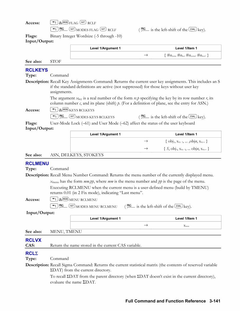
Full Command and Function Reference 3-141
Access: &HFLAG L RCLF °LMODES FLAG L RCLF ( °is the left-shift of the Nkey). Flags: Binary Integer Wordsize (-5 through -10) Input/Output:
Level 1/Argument 1 Level 1/Item 1
→ #nsystem #nuser #nsystem2 #nuser2 See also: STOF
RCLKEYS Type: Command Description: Recall Key Assignments Command: Returns the current user key assignments. This includes an S
if the standard definitions are active (not suppressed) for those keys without user key assignments.
The argument xkey is a real number of the form rc.p specifying the key by its row number r, its column number c, and its plane (shift) p. (For a definition of plane, see the entry for ASN.)
Access: &HKEYS RCLKEYS °LMODES KEYS RCLKEYS ( °is the left-shift of the Nkey). Flags: User-Mode Lock (61) and User Mode (62) affect the status of the user keyboard Input/Output:
Level 1/Argument 1 Level 1/Item 1
→ obj1, xkey 1, ... ,objn, xkey n
→ S, obj1, xkey 1, ... objn, xkey n See also: ASN, DELKEYS, STOKEYS
RCLMENU Type: Command Description: Recall Menu Number Command: Returns the menu number of the currently displayed menu. xmenu has the form mm.pp, where mm is the menu number and pp is the page of the menu. Executing RCLMENU when the current menu is a user-defined menu (build by TMENU)
returns 0.01 (in 2 Fix mode), indicating Last menu. Access: &HMENU RCLMENU °LMODES MENU RCLMENU ( °is the left-shift of the Nkey). Input/Output:
Level 1/Argument 1 Level 1/Item 1
→ xmenu See also: MENU, TMENU
RCLVX CAS: Return the name stored in the current CAS variable.
RCLΣ Type: Command Description: Recall Sigma Command: Returns the current statistical matrix (the contents of reserved variable
ΣDAT) from the current directory. To recall ΣDAT from the parent directory (when ΣDAT doesn't exist in the current directory),
evaluate the name ΣDAT.
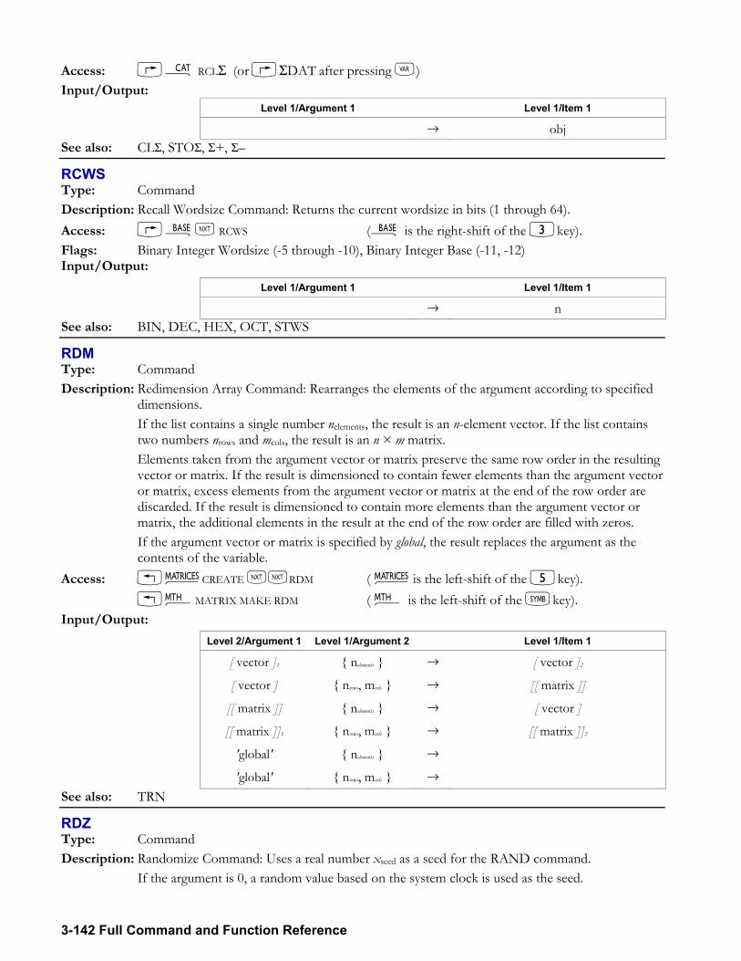
3-142 Full Command and Function Reference
Access: µ RCLΣ (or ΣDAT after pressing J) Input/Output:
Level 1/Argument 1 Level 1/Item 1
→ obj See also: CLΣ, STOΣ, Σ+, Σ
RCWS Type: Command Description: Recall Wordsize Command: Returns the current wordsize in bits (1 through 64). Access: ãL RCWS (ã is the right-shift of the 3key). Flags: Binary Integer Wordsize (-5 through -10), Binary Integer Base (-11, -12) Input/Output:
Level 1/Argument 1 Level 1/Item 1
→ n See also: BIN, DEC, HEX, OCT, STWS
RDM Type: Command Description: Redimension Array Command: Rearranges the elements of the argument according to specified
dimensions. If the list contains a single number nelements, the result is an n-element vector. If the list contains
two numbers nrows and mcols, the result is an n × m matrix. Elements taken from the argument vector or matrix preserve the same row order in the resulting
vector or matrix. If the result is dimensioned to contain fewer elements than the argument vector or matrix, excess elements from the argument vector or matrix at the end of the row order are discarded. If the result is dimensioned to contain more elements than the argument vector or matrix, the additional elements in the result at the end of the row order are filled with zeros.
If the argument vector or matrix is specified by global, the result replaces the argument as the contents of the variable.
Access: !Ø CREATE LLRDM ( Ø is the left-shift of the 5key). !´MATRIX MAKE RDM ( ´ is the left-shift of the Pkey). Input/Output:
Level 2/Argument 1 Level 1/Argument 2 Level 1/Item 1
[ vector ]1 nelements → [ vector ]2
[ vector ] nrows, mcols → [[ matrix ]]
[[ matrix ]] nelements → [ vector ]
[[ matrix ]]1 nrows, mcols → [[ matrix ]]2
'global' nelements →
'global' nrows, mcols → See also: TRN
RDZ Type: Command Description: Randomize Command: Uses a real number xseed as a seed for the RAND command. If the argument is 0, a random value based on the system clock is used as the seed.
Full Command and Function Reference 3-143
Access: !´LPROBABILITY RDZ ( ´ is the left-shift of the Pkey). Input/Output:
Level 1/Argument 1 Level 1/Item 1
xseed → See also: COMB, PERM, RAND, !
RE Type: Function Description: Real Part Function: Returns the real part of the argument. If the argument is a vector or matrix, RE returns a real array, the elements of which are equal to
the real parts of the corresponding elements of the argument array. Access: ßL RE (ßis the right-shift of the 1key). Flags: Numerical Results (-3) Input/Output:
Level 1/Argument 1 Level 1/Item 1
x → x
x_unit → x
(x,y) → x
[ R-array ] → [ R-array ] [ C-array ] → [ R-array ]
'symb' → 'RE(symb') See also: C→R, IM, R→C
RECN Type: Command Description: Receive Renamed Object Command: Prepares the hp49g+/hp48gII to receive a file from
another Kermit server device, and to store the file in a specified variable. RECN is identical to RECV except that the name under which the received data is stored is
specified. Access: µ RECN Flags: I/O Device flag (-33), I/O Data Format (-35), RECV Overwrite (-36), I/O Messages (-39) Input/Output:
Level 1/Argument 1 Level 1/Item 1
'name' → name →
See also: BAUD, CKSM, CLOSEIO, FINISH, KERRM, KGET, PARITY, RECV, SEND, SERVER, TRANSIO
RECT Type: Command Description: Rectangular Mode Command: Sets Rectangular coordinate mode. RECT clears flags 15 and 16. In Rectangular mode, vectors are displayed as rectangular components. Therefore, a 3D vector
would appear as [X Y Z].
3-144 Full Command and Function Reference
Access: &H ANGLE RECT ´VECTOR L RECT ( ´is the left-shift of the Pkey). °L MODES ANGLE RECT ( °is the left-shift of the Nkey). Input/Output: None See also: CYLIN, SPHERE
RECV Type: Command Description: Receive Object Command: Instructs the hp49g+/hp48gII to look for a named file from another
Kermit server device. The received file is stored in a variable named by the sender. Since the hp49g+/hp48gII does not normally look for incoming Kermit files, you must use
RECV to tell it to do so. Access: µ RECV Flags: I/O Device flag (-33), I/O Data Format (-35), RECV Overwrite (-36), I/O Messages (-39) Input/Output: None See also: BAUD, CKSM, FINISH, KGET, PARITY, RECN, SEND, SERVER, TRANSIO
REF CAS: Reduce a matrix to echelon form. This is a subdiagonal reduction (Gauss, not Gauss-Jordan).
REMAINDER CAS: Return the remainder of the Euclidean division of two polynomials.
RENAME Type: Command Description: Rename Object Command: Renames an object to the name that you specify. Access: µ RENAME Input/Output:
Level 2/Argument 1 Level 1/Argument 2 Level 1/Item 1
new 'name' old 'name' → See also: COPY
REORDER CAS: Rewrite a polynomial expression in increasing or decreasing order of powers.
REPEAT Type: Command Description: REPEAT Command: Starts loop clause in WHILE REPEAT END indefinite loop
structure. See the WHILE entry for more information. Access: !°BRANCH WHILE REPEAT ( °is the left-shift of the Nkey). Input/Output: None See also: END, WHILE
REPL Type: Command Description: Replace Command: Replaces a portion of the target object (first input) with a specified object
(third input), beginning at a specified position (second input).
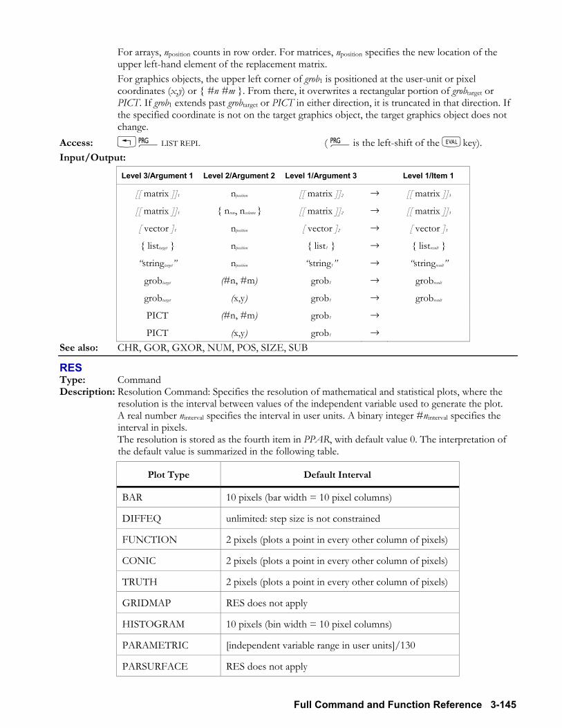
Full Command and Function Reference 3-145
For arrays, nposition counts in row order. For matrices, nposition specifies the new location of the upper left-hand element of the replacement matrix.
For graphics objects, the upper left corner of grob1 is positioned at the user-unit or pixel coordinates (x,y) or #n #m . From there, it overwrites a rectangular portion of grobtarget or PICT. If grob1 extends past grobtarget or PICT in either direction, it is truncated in that direction. If the specified coordinate is not on the target graphics object, the target graphics object does not change.
Access: !°LIST REPL ( °is the left-shift of the Nkey). Input/Output:
Level 3/Argument 1 Level 2/Argument 2 Level 1/Argument 3 Level 1/Item 1
[[ matrix ]]1 nposition [[ matrix ]]2 → [[ matrix ]]3
[[ matrix ]]1 nrow, ncolumn [[ matrix ]]2 → [[ matrix ]]3
[ vector ]1 nposition [ vector ]2 → [ vector ]3
listtarget nposition list1 → listresult
stringtarget nposition string1 → stringresult
grobtarget (#n, #m) grob1 → grobresult
grobtarget (x,y) grob1 → grobresult
PICT (#n, #m) grob1 →
PICT (x,y) grob1 → See also: CHR, GOR, GXOR, NUM, POS, SIZE, SUB
RES Type: Command Description: Resolution Command: Specifies the resolution of mathematical and statistical plots, where the
resolution is the interval between values of the independent variable used to generate the plot. A real number ninterval specifies the interval in user units. A binary integer #ninterval specifies the
interval in pixels. The resolution is stored as the fourth item in PPAR, with default value 0. The interpretation of
the default value is summarized in the following table.
Plot Type Default Interval
BAR 10 pixels (bar width = 10 pixel columns)
DIFFEQ unlimited: step size is not constrained
FUNCTION 2 pixels (plots a point in every other column of pixels)
CONIC 2 pixels (plots a point in every other column of pixels)
TRUTH 2 pixels (plots a point in every other column of pixels)
GRIDMAP RES does not apply
HISTOGRAM 10 pixels (bin width = 10 pixel columns)
PARAMETRIC [independent variable range in user units]/130
PARSURFACE RES does not apply
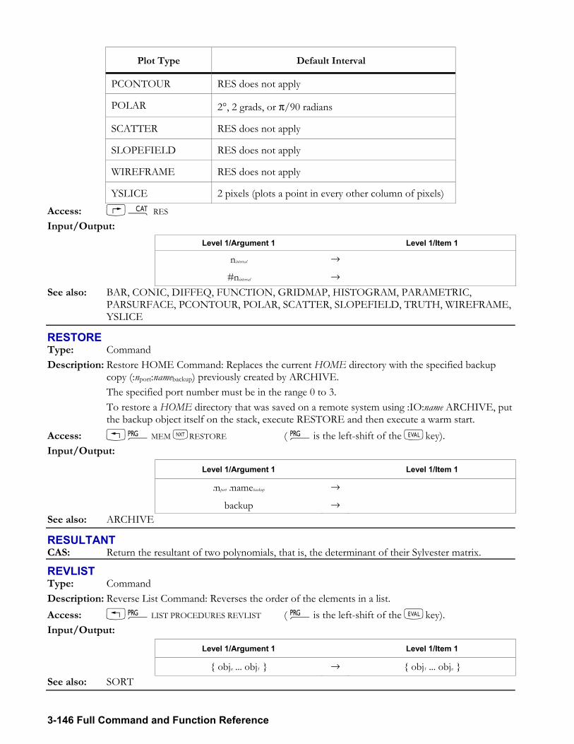
3-146 Full Command and Function Reference
Plot Type Default Interval
PCONTOUR RES does not apply
POLAR 2°, 2 grads, or π/90 radians
SCATTER RES does not apply
SLOPEFIELD RES does not apply
WIREFRAME RES does not apply
YSLICE 2 pixels (plots a point in every other column of pixels)
Access: µ RES Input/Output:
Level 1/Argument 1 Level 1/Item 1
ninterval →
#ninterval → See also: BAR, CONIC, DIFFEQ, FUNCTION, GRIDMAP, HISTOGRAM, PARAMETRIC,
PARSURFACE, PCONTOUR, POLAR, SCATTER, SLOPEFIELD, TRUTH, WIREFRAME, YSLICE
RESTORE Type: Command Description: Restore HOME Command: Replaces the current HOME directory with the specified backup
copy (:nport:namebackup) previously created by ARCHIVE. The specified port number must be in the range 0 to 3. To restore a HOME directory that was saved on a remote system using :IO:name ARCHIVE, put
the backup object itself on the stack, execute RESTORE and then execute a warm start. Access: °MEM LRESTORE ( °is the left-shift of the Nkey). Input/Output:
Level 1/Argument 1 Level 1/Item 1
:nport :namebackup →
backup → See also: ARCHIVE
RESULTANT CAS: Return the resultant of two polynomials, that is, the determinant of their Sylvester matrix.
REVLIST Type: Command Description: Reverse List Command: Reverses the order of the elements in a list. Access: !°LIST PROCEDURES REVLIST ( °is the left-shift of the Nkey). Input/Output:
Level 1/Argument 1 Level 1/Item 1
objn ... obj1 → obj1 ... objn See also: SORT
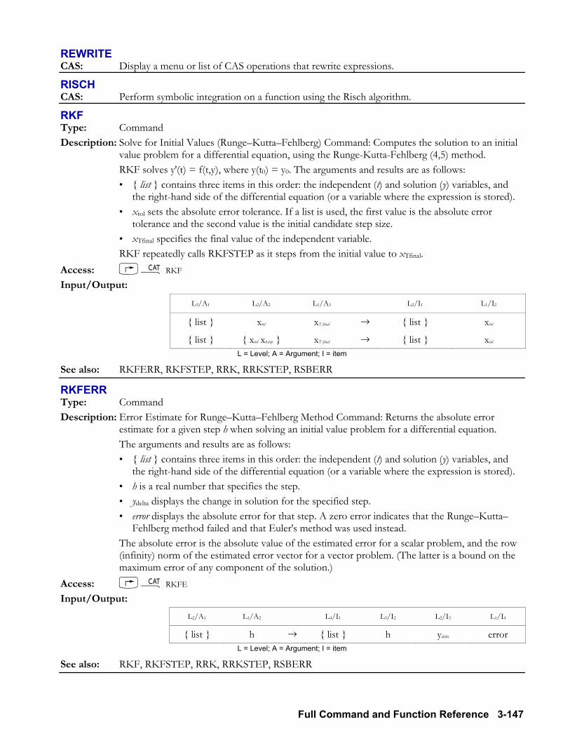
Full Command and Function Reference 3-147
REWRITE CAS: Display a menu or list of CAS operations that rewrite expressions.
RISCH CAS: Perform symbolic integration on a function using the Risch algorithm.
RKF Type: Command Description: Solve for Initial Values (RungeKuttaFehlberg) Command: Computes the solution to an initial
value problem for a differential equation, using the Runge-Kutta-Fehlberg (4,5) method. RKF solves y'(t) = f(t,y), where y(t0) = y0. The arguments and results are as follows:
list contains three items in this order: the independent (t) and solution (y) variables, and the right-hand side of the differential equation (or a variable where the expression is stored).
xtol sets the absolute error tolerance. If a list is used, the first value is the absolute error tolerance and the second value is the initial candidate step size.
xTfinal specifies the final value of the independent variable. RKF repeatedly calls RKFSTEP as it steps from the initial value to xTfinal. Access: µ RKF Input/Output:
L3/A1 L2/A2 L1/A3 L2/I1 L1/I2
list xtol xT final → list xtol
list xtol xhstep xT final → list xtol L = Level; A = Argument; I = item
See also: RKFERR, RKFSTEP, RRK, RRKSTEP, RSBERR
RKFERR Type: Command Description: Error Estimate for RungeKuttaFehlberg Method Command: Returns the absolute error
estimate for a given step h when solving an initial value problem for a differential equation. The arguments and results are as follows:
list contains three items in this order: the independent (t) and solution (y) variables, and the right-hand side of the differential equation (or a variable where the expression is stored).
h is a real number that specifies the step. ydelta displays the change in solution for the specified step. error displays the absolute error for that step. A zero error indicates that the RungeKutta
Fehlberg method failed and that Euler's method was used instead. The absolute error is the absolute value of the estimated error for a scalar problem, and the row
(infinity) norm of the estimated error vector for a vector problem. (The latter is a bound on the maximum error of any component of the solution.)
Access: µ RKFE Input/Output:
L2/A1 L1/A2 L4/I1 L3/I2 L2/I3 L1/I4
list h → list h ydelta error L = Level; A = Argument; I = item
See also: RKF, RKFSTEP, RRK, RRKSTEP, RSBERR
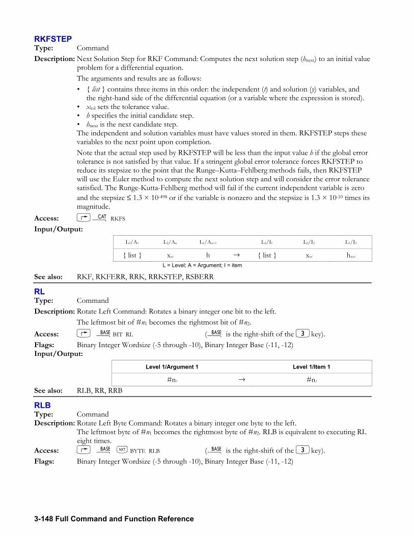
3-148 Full Command and Function Reference
RKFSTEP Type: Command Description: Next Solution Step for RKF Command: Computes the next solution step (hnext) to an initial value
problem for a differential equation. The arguments and results are as follows:
list contains three items in this order: the independent (t) and solution (y) variables, and the right-hand side of the differential equation (or a variable where the expression is stored).
xtol sets the tolerance value. h specifies the initial candidate step. hnext is the next candidate step.
The independent and solution variables must have values stored in them. RKFSTEP steps these variables to the next point upon completion.
Note that the actual step used by RKFSTEP will be less than the input value h if the global error tolerance is not satisfied by that value. If a stringent global error tolerance forces RKFSTEP to reduce its stepsize to the point that the RungeKuttaFehlberg methods fails, then RKFSTEP will use the Euler method to compute the next solution step and will consider the error tolerance satisfied. The Runge-Kutta-Fehlberg method will fail if the current independent variable is zero and the stepsize ≤ 1.3 × 10-498 or if the variable is nonzero and the stepsize is 1.3 × 10⁻¹⁰ times its magnitude.
Access: µ RKFS Input/Output:
L3/A1 L2/An L1/An+1 L3/I1 L2/I2 L1/I3
list xtol h → list xtol hnext L = Level; A = Argument; I = item
See also: RKF, RKFERR, RRK, RRKSTEP, RSBERR
RL Type: Command Description: Rotate Left Command: Rotates a binary integer one bit to the left. The leftmost bit of #n1 becomes the rightmost bit of #n2. Access: ãBIT RL (ã is the right-shift of the 3key). Flags: Binary Integer Wordsize (-5 through -10), Binary Integer Base (-11, -12) Input/Output:
Level 1/Argument 1 Level 1/Item 1
#n1 → #n2 See also: RLB, RR, RRB
RLB Type: Command Description: Rotate Left Byte Command: Rotates a binary integer one byte to the left. The leftmost byte of #n1 becomes the rightmost byte of #n2. RLB is equivalent to executing RL
eight times. Access: ã L BYTE RLB (ã is the right-shift of the 3key). Flags: Binary Integer Wordsize (-5 through -10), Binary Integer Base (-11, -12)
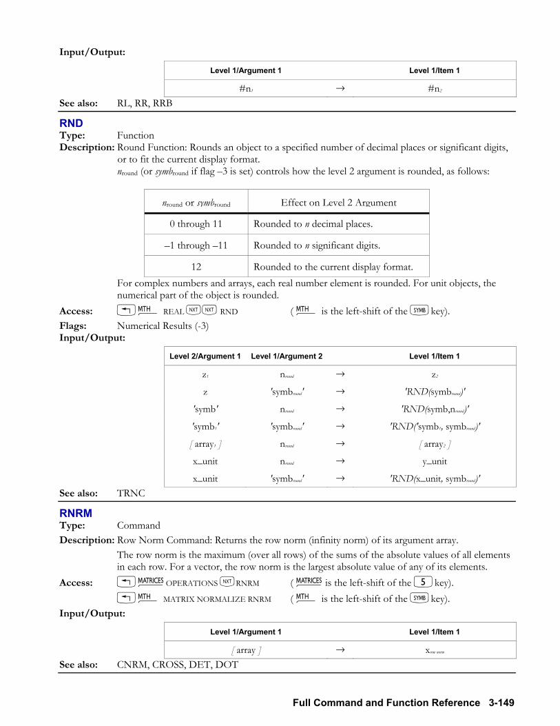
Full Command and Function Reference 3-149
Input/Output:
Level 1/Argument 1 Level 1/Item 1
#n1 → #n2 See also: RL, RR, RRB
RND Type: Function Description: Round Function: Rounds an object to a specified number of decimal places or significant digits,
or to fit the current display format. nround (or symbround if flag 3 is set) controls how the level 2 argument is rounded, as follows:
nround or symbround Effect on Level 2 Argument
0 through 11 Rounded to n decimal places.
1 through 11 Rounded to n significant digits.
12 Rounded to the current display format. For complex numbers and arrays, each real number element is rounded. For unit objects, the
numerical part of the object is rounded. Access: !´ REAL LL RND ( ´ is the left-shift of the Pkey). Flags: Numerical Results (-3) Input/Output:
Level 2/Argument 1 Level 1/Argument 2 Level 1/Item 1
z1 nround → z2
z 'symbround' → 'RND(symbround)'
'symb' nround → 'RND(symb,nround)'
'symb1' 'symbround' → 'RND('symb1, symbround)'
[ array1 ] nround → [ array2 ]
x_unit nround → y_unit
x_unit 'symbround' → 'RND(x_unit, symbround)' See also: TRNC
RNRM Type: Command Description: Row Norm Command: Returns the row norm (infinity norm) of its argument array. The row norm is the maximum (over all rows) of the sums of the absolute values of all elements
in each row. For a vector, the row norm is the largest absolute value of any of its elements. Access: !Ø OPERATIONS LRNRM ( Ø is the left-shift of the 5key). !´ MATRIX NORMALIZE RNRM ( ´ is the left-shift of the Pkey). Input/Output:
Level 1/Argument 1 Level 1/Item 1
[ array ] → xrow norm See also: CNRM, CROSS, DET, DOT
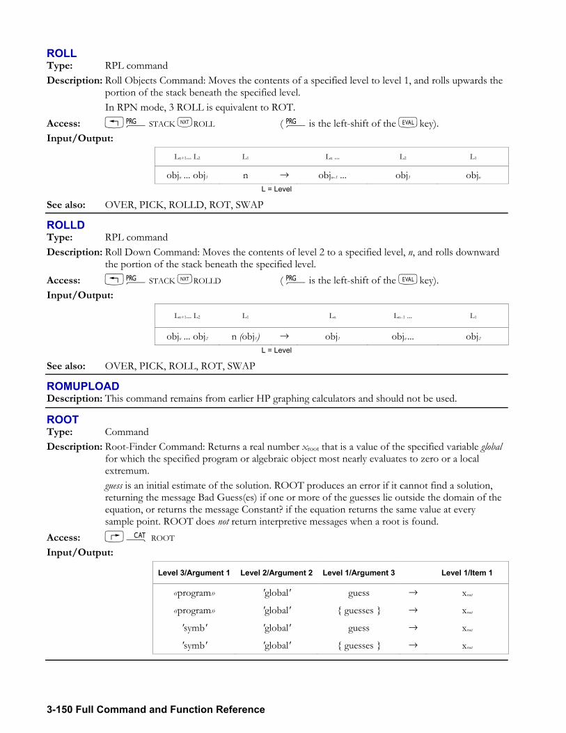
3-150 Full Command and Function Reference
ROLL Type: RPL command Description: Roll Objects Command: Moves the contents of a specified level to level 1, and rolls upwards the
portion of the stack beneath the specified level. In RPN mode, 3 ROLL is equivalent to ROT. Access: !°STACK LROLL ( °is the left-shift of the Nkey). Input/Output:
Ln+1... L2 L1 Ln ... L2 L1
objn ... obj1 n → objn1 ... obj1 objn L = Level
See also: OVER, PICK, ROLLD, ROT, SWAP
ROLLD Type: RPL command Description: Roll Down Command: Moves the contents of level 2 to a specified level, n, and rolls downward
the portion of the stack beneath the specified level. Access: !°STACK LROLLD ( °is the left-shift of the Nkey). Input/Output:
Ln+1... L2 L1 Ln Ln1 ... L1
objn ... obj2 n (obj1) → obj1 objn ... obj2 L = Level
See also: OVER, PICK, ROLL, ROT, SWAP
ROMUPLOAD Description: This command remains from earlier HP graphing calculators and should not be used.
ROOT Type: Command Description: Root-Finder Command: Returns a real number xroot that is a value of the specified variable global
for which the specified program or algebraic object most nearly evaluates to zero or a local extremum.
guess is an initial estimate of the solution. ROOT produces an error if it cannot find a solution, returning the message Bad Guess(es) if one or more of the guesses lie outside the domain of the equation, or returns the message Constant? if the equation returns the same value at every sample point. ROOT does not return interpretive messages when a root is found.
Access: µ ROOT Input/Output:
Level 3/Argument 1 Level 2/Argument 2 Level 1/Argument 3 Level 1/Item 1
«program» 'global' guess → xroot
«program» 'global' guesses → xroot
'symb' 'global' guess → xroot
'symb' 'global' guesses → xroot
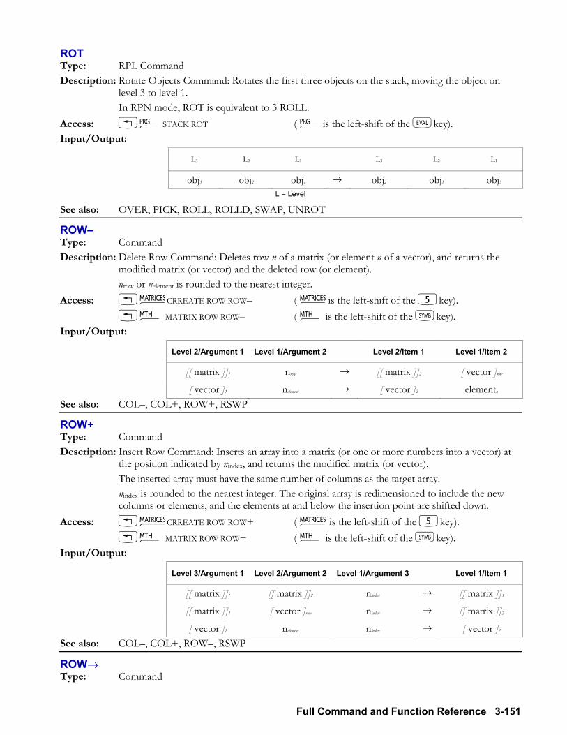
Full Command and Function Reference 3-151
ROT Type: RPL Command Description: Rotate Objects Command: Rotates the first three objects on the stack, moving the object on
level 3 to level 1. In RPN mode, ROT is equivalent to 3 ROLL. Access: !°STACK ROT ( °is the left-shift of the Nkey). Input/Output:
L3 L2 L1 L3 L2 L1
obj3 obj2 obj1 → obj2 obj1 obj3 L = Level
See also: OVER, PICK, ROLL, ROLLD, SWAP, UNROT
ROW Type: Command Description: Delete Row Command: Deletes row n of a matrix (or element n of a vector), and returns the
modified matrix (or vector) and the deleted row (or element). nrow or nelement is rounded to the nearest integer. Access: !Ø CRREATE ROW ROW ( Ø is the left-shift of the 5key). !´ MATRIX ROW ROW ( ´ is the left-shift of the Pkey). Input/Output:
Level 2/Argument 1 Level 1/Argument 2 Level 2/Item 1 Level 1/Item 2
[[ matrix ]]1 nrow → [[ matrix ]]2 [ vector ]row
[ vector ]1 nelement → [ vector ]2 elementn See also: COL, COL+, ROW+, RSWP
ROW+ Type: Command Description: Insert Row Command: Inserts an array into a matrix (or one or more numbers into a vector) at
the position indicated by nindex, and returns the modified matrix (or vector). The inserted array must have the same number of columns as the target array. nindex is rounded to the nearest integer. The original array is redimensioned to include the new
columns or elements, and the elements at and below the insertion point are shifted down. Access: !Ø CRREATE ROW ROW+ ( Ø is the left-shift of the 5key). !´ MATRIX ROW ROW+ ( ´ is the left-shift of the Pkey). Input/Output:
Level 3/Argument 1 Level 2/Argument 2 Level 1/Argument 3 Level 1/Item 1
[[ matrix ]]1 [[ matrix ]]2 nindex → [[ matrix ]]3
[[ matrix ]]1 [ vector ]row nindex → [[ matrix ]]2
[ vector ]1 nelement nindex → [ vector ]2 See also: COL, COL+, ROW, RSWP
ROW→ Type: Command
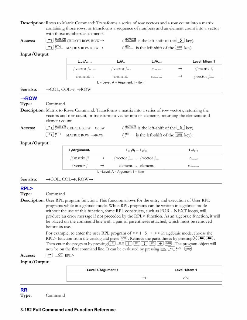
3-152 Full Command and Function Reference
Description: Rows to Matrix Command: Transforms a series of row vectors and a row count into a matrix containing those rows, or transforms a sequence of numbers and an element count into a vector with those numbers as elements.
Access: !Ø CREATE ROW ROW→ ( Ø is the left-shift of the 5key). !´ MATRIX ROW ROW→ ( ´ is the left-shift of the Pkey). Input/Output:
Ln+1/A1 L2/An L1/An+1 Level 1/Item 1 [ vector ]row 1 … [ vector ]row n nrow count → [[ matrix ]]
element1 … elementn nelement count → [ vector ]column L = Level; A = Argument; I = item
See also: →COL, COL→, →ROW
→ROW Type: Command Description: Matrix to Rows Command: Transforms a matrix into a series of row vectors, returning the
vectors and row count, or transforms a vector into its elements, returning the elements and element count.
Access: !Ø CREATE ROW →ROW ( Ø is the left-shift of the 5key). !´ MATRIX ROW →ROW ( ´ is the left-shift of the Pkey).
Input/Output: L1/Argument1 Ln+1/I1 L2/In L1/In+1
[[ matrix ]] → [ vector ]row n [ vector ]row n nrowcount
[ vector ] → element1 elementn nelementcount L =Level; A = Argument; I = Item
See also: →COL, COL→, ROW→
RPL> Type: Command Description: User RPL program function. This function allows for the entry and execution of User RPL
programs while in algebraic mode. While RPL programs can be written in algebraic mode without the use of this function, some RPL constructs, such as FORNEXT loops, will produce an error message if not preceded by the RPL> function. As an algebraic function, it will be placed on the command line with a pair of parentheses attached, which must be removed before its use.
For example, to enter the user RPL program of << 1 5 + >> in algebraic mode, choose the RPL> function from the catalog and press `. Remove the parentheses by pressing . Then enter the program by pressing å1#5#+`. The program object will now be on the first command line. It can be evaluated by pressing N!î`.
Access: µ RPL> Input/Output:
Level 1/Argument 1 Level 1/Item 1
→ obj
RR Type: Command
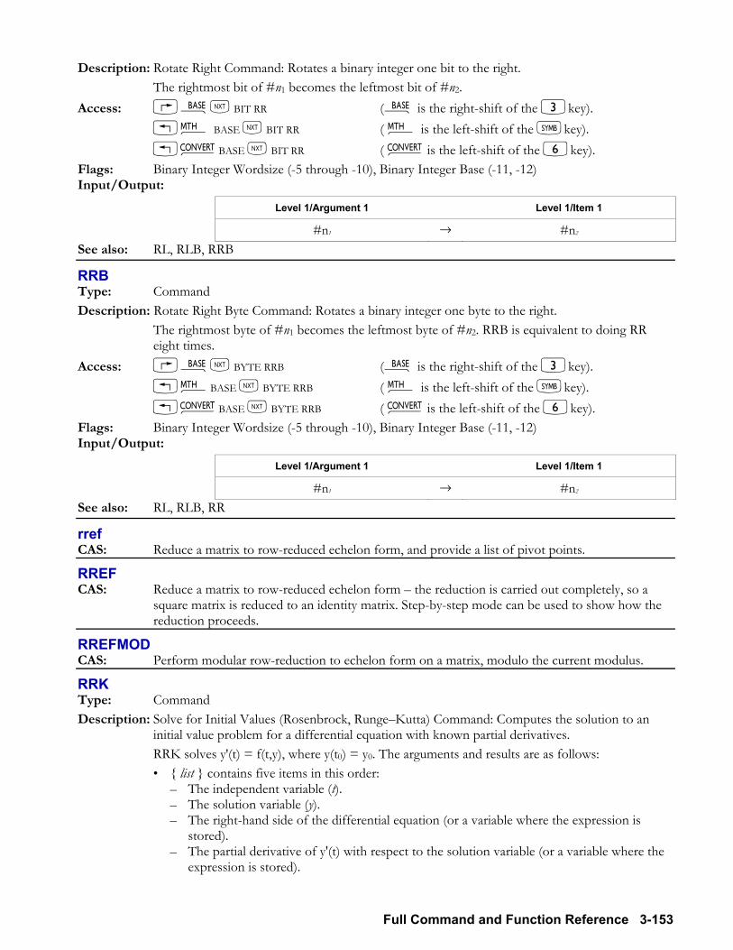
Full Command and Function Reference 3-153
Description: Rotate Right Command: Rotates a binary integer one bit to the right. The rightmost bit of #n1 becomes the leftmost bit of #n2. Access: ãL BIT RR (ã is the right-shift of the 3key). !´ BASE L BIT RR ( ´ is the left-shift of the Pkey). !Ú BASE L BIT RR ( Ú is the left-shift of the 6key). Flags: Binary Integer Wordsize (-5 through -10), Binary Integer Base (-11, -12) Input/Output:
Level 1/Argument 1 Level 1/Item 1
#n1 → #n2 See also: RL, RLB, RRB
RRB Type: Command Description: Rotate Right Byte Command: Rotates a binary integer one byte to the right. The rightmost byte of #n1 becomes the leftmost byte of #n2. RRB is equivalent to doing RR
eight times. Access: ãL BYTE RRB (ã is the right-shift of the 3key). !´BASE L BYTE RRB ( ´ is the left-shift of the Pkey). !Ú BASE L BYTE RRB ( Ú is the left-shift of the 6key). Flags: Binary Integer Wordsize (-5 through -10), Binary Integer Base (-11, -12) Input/Output:
Level 1/Argument 1 Level 1/Item 1
#n1 → #n2 See also: RL, RLB, RR
rref CAS: Reduce a matrix to row-reduced echelon form, and provide a list of pivot points.
RREF CAS: Reduce a matrix to row-reduced echelon form the reduction is carried out completely, so a
square matrix is reduced to an identity matrix. Step-by-step mode can be used to show how the reduction proceeds.
RREFMOD CAS: Perform modular row-reduction to echelon form on a matrix, modulo the current modulus.
RRK Type: Command Description: Solve for Initial Values (Rosenbrock, RungeKutta) Command: Computes the solution to an
initial value problem for a differential equation with known partial derivatives. RRK solves y'(t) = f(t,y), where y(t0) = y0. The arguments and results are as follows:
list contains five items in this order: The independent variable (t). The solution variable (y). The right-hand side of the differential equation (or a variable where the expression is
stored). The partial derivative of y'(t) with respect to the solution variable (or a variable where the
expression is stored).
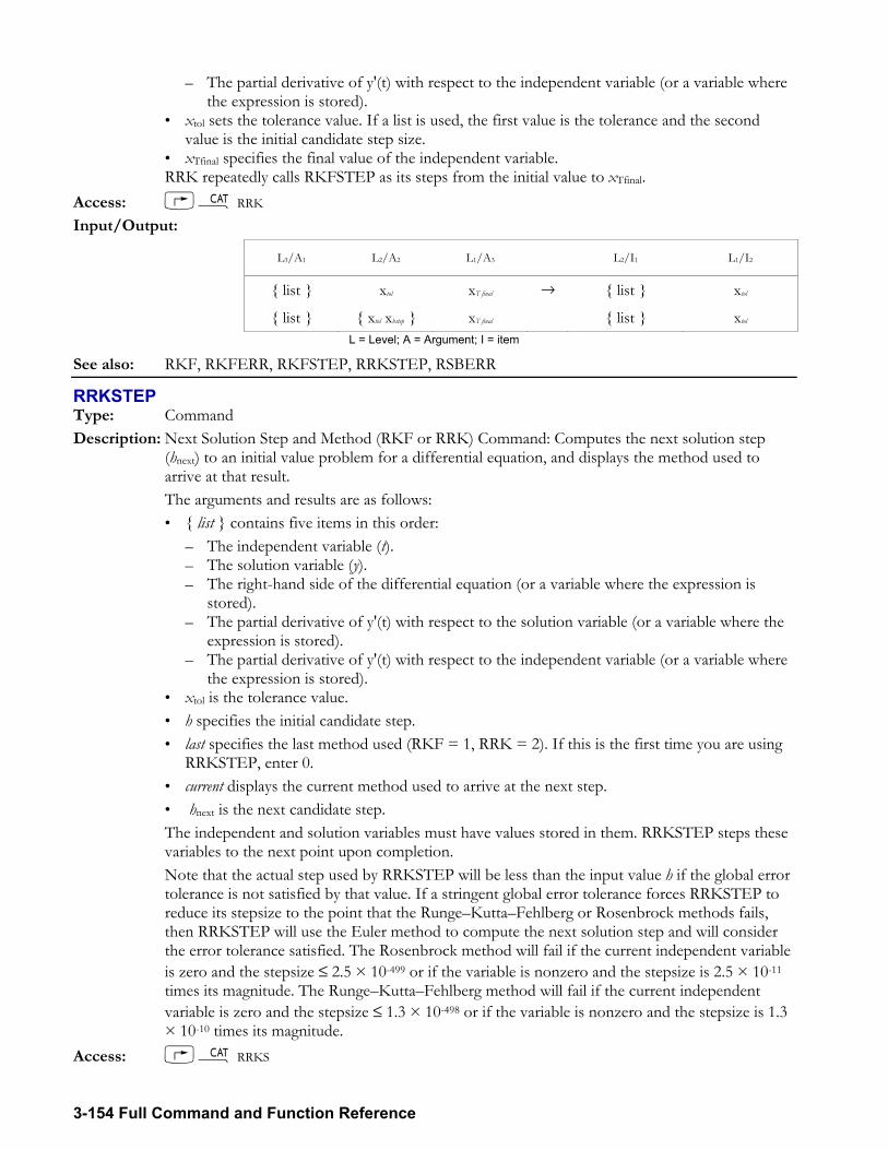
3-154 Full Command and Function Reference
The partial derivative of y'(t) with respect to the independent variable (or a variable where the expression is stored).
xtol sets the tolerance value. If a list is used, the first value is the tolerance and the second value is the initial candidate step size.
xTfinal specifies the final value of the independent variable. RRK repeatedly calls RKFSTEP as its steps from the initial value to xTfinal. Access: µ RRK Input/Output:
L3/A1 L2/A2 L1/A3 L2/I1 L1/I2
list xtol xT final → list xtol
list xtol xhstep xT final list xtol L = Level; A = Argument; I = item
See also: RKF, RKFERR, RKFSTEP, RRKSTEP, RSBERR
RRKSTEP Type: Command Description: Next Solution Step and Method (RKF or RRK) Command: Computes the next solution step
(hnext) to an initial value problem for a differential equation, and displays the method used to arrive at that result.
The arguments and results are as follows: list contains five items in this order:
The independent variable (t). The solution variable (y). The right-hand side of the differential equation (or a variable where the expression is
stored). The partial derivative of y'(t) with respect to the solution variable (or a variable where the
expression is stored). The partial derivative of y'(t) with respect to the independent variable (or a variable where
the expression is stored). xtol is the tolerance value. h specifies the initial candidate step. last specifies the last method used (RKF = 1, RRK = 2). If this is the first time you are using
RRKSTEP, enter 0. current displays the current method used to arrive at the next step. hnext is the next candidate step.
The independent and solution variables must have values stored in them. RRKSTEP steps these variables to the next point upon completion.
Note that the actual step used by RRKSTEP will be less than the input value h if the global error tolerance is not satisfied by that value. If a stringent global error tolerance forces RRKSTEP to reduce its stepsize to the point that the RungeKuttaFehlberg or Rosenbrock methods fails, then RRKSTEP will use the Euler method to compute the next solution step and will consider the error tolerance satisfied. The Rosenbrock method will fail if the current independent variable is zero and the stepsize ≤ 2.5 × 10-499 or if the variable is nonzero and the stepsize is 2.5 × 10⁻¹¹ times its magnitude. The RungeKuttaFehlberg method will fail if the current independent variable is zero and the stepsize ≤ 1.3 × 10-498 or if the variable is nonzero and the stepsize is 1.3 × 10⁻¹⁰ times its magnitude.
Access: µ RRKS
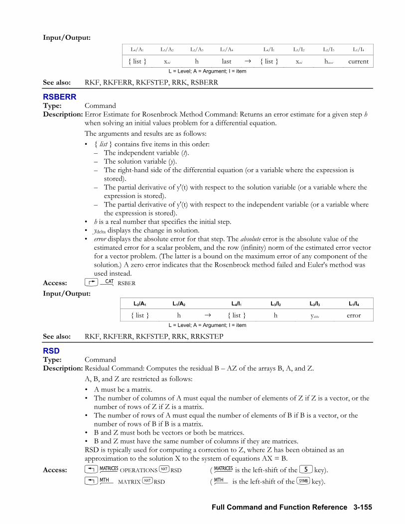
Full Command and Function Reference 3-155
Input/Output: L4/A1 L3/A2 L2/A3 L1/A4 L4/I1 L3/I2 L2/I3 L1/I4
list xtol h last → list xtol hnext currentL = Level; A = Argument; I = item
See also: RKF, RKFERR, RKFSTEP, RRK, RSBERR
RSBERR Type: Command Description: Error Estimate for Rosenbrock Method Command: Returns an error estimate for a given step h
when solving an initial values problem for a differential equation. The arguments and results are as follows:
list contains five items in this order: The independent variable (t). The solution variable (y). The right-hand side of the differential equation (or a variable where the expression is
stored). The partial derivative of y'(t) with respect to the solution variable (or a variable where the
expression is stored). The partial derivative of y'(t) with respect to the independent variable (or a variable where
the expression is stored). h is a real number that specifies the initial step. ydelta displays the change in solution. error displays the absolute error for that step. The absolute error is the absolute value of the
estimated error for a scalar problem, and the row (infinity) norm of the estimated error vector for a vector problem. (The latter is a bound on the maximum error of any component of the solution.) A zero error indicates that the Rosenbrock method failed and Euler's method was used instead.
Access: µ RSBER Input/Output:
L2/A1 L1/A2 L4/I1 L3/I2 L2/I3 L1/I4 list h → list h ydelta error
L = Level; A = Argument; I = item
See also: RKF, RKFERR, RKFSTEP, RRK, RRKSTEP
RSD Type: Command Description: Residual Command: Computes the residual B AZ of the arrays B, A, and Z. A, B, and Z are restricted as follows:
A must be a matrix. The number of columns of A must equal the number of elements of Z if Z is a vector, or the
number of rows of Z if Z is a matrix. The number of rows of A must equal the number of elements of B if B is a vector, or the
number of rows of B if B is a matrix. B and Z must both be vectors or both be matrices. B and Z must have the same number of columns if they are matrices.
RSD is typically used for computing a correction to Z, where Z has been obtained as an approximation to the solution X to the system of equations AX = B.
Access: !Ø OPERATIONS LRSD ( Ø is the left-shift of the 5key). !´ MATRIX LRSD ( ´ is the left-shift of the Pkey).
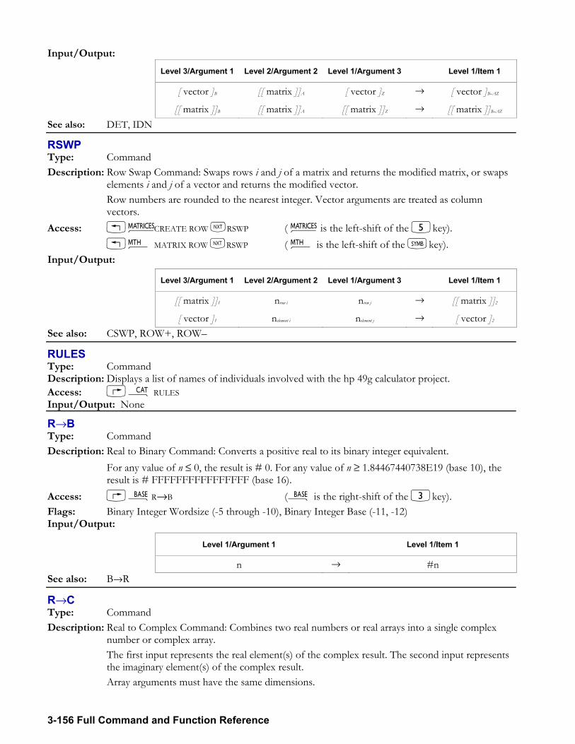
3-156 Full Command and Function Reference
Input/Output: Level 3/Argument 1 Level 2/Argument 2 Level 1/Argument 3 Level 1/Item 1
[ vector ]B [[ matrix ]]A [ vector ]Z → [ vector ]BAZ
[[ matrix ]]B [[ matrix ]]A [[ matrix ]]Z → [[ matrix ]]BAZ See also: DET, IDN
RSWP Type: Command Description: Row Swap Command: Swaps rows i and j of a matrix and returns the modified matrix, or swaps
elements i and j of a vector and returns the modified vector. Row numbers are rounded to the nearest integer. Vector arguments are treated as column
vectors. Access: !Ø CREATE ROW LRSWP ( Ø is the left-shift of the 5key). !´ MATRIX ROW LRSWP ( ´ is the left-shift of the Pkey). Input/Output:
Level 3/Argument 1 Level 2/Argument 2 Level 1/Argument 3 Level 1/Item 1
[[ matrix ]]1 nrow i nrow j → [[ matrix ]]2
[ vector ]1 nelement i nelement j → [ vector ]2 See also: CSWP, ROW+, ROW
RULES Type: Command Description: Displays a list of names of individuals involved with the hp 49g calculator project. Access: µ RULES Input/Output: None
R→B Type: Command Description: Real to Binary Command: Converts a positive real to its binary integer equivalent. For any value of n ≤ 0, the result is # 0. For any value of n ≥ 1.84467440738E19 (base 10), the
result is # FFFFFFFFFFFFFFFF (base 16). Access: ãR→B (ã is the right-shift of the 3key). Flags: Binary Integer Wordsize (-5 through -10), Binary Integer Base (-11, -12) Input/Output:
Level 1/Argument 1 Level 1/Item 1
n → #n See also: B→R
R→C Type: Command Description: Real to Complex Command: Combines two real numbers or real arrays into a single complex
number or complex array. The first input represents the real element(s) of the complex result. The second input represents
the imaginary element(s) of the complex result. Array arguments must have the same dimensions.
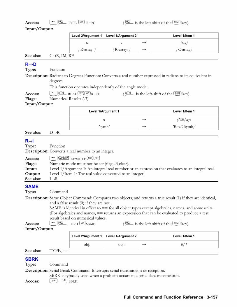
Full Command and Function Reference 3-157
Access: !°TYPE L R→C ( °is the left-shift of the Nkey). Input/Output:
Level 2/Argument 1 Level 1/Argument 2 Level 1/Item 1
x y → (x,y) [ R-array1 ] [ R-array2 ] → [ C-array ]
See also: C→R, IM, RE
R→D Type: Function Description: Radians to Degrees Function: Converts a real number expressed in radians to its equivalent in
degrees. This function operates independently of the angle mode. Access: !´REAL LLR→D ( ´ is the left-shift of the Pkey). Flags: Numerical Results (-3) Input/Output:
Level 1/Argument 1 Level 1/Item 1
x → (180/π)x 'symb' → 'R→D(symb)'
See also: D→R
R→I Type: Function Description: Converts a real number to an integer.
Access: !Ú REWRITE LL Flags: Numeric mode must not be set (flag 3 clear). Input: Level 1/Argument 1: An integral real number or an expression that evaluates to an integral real. Output: Level 1/Item 1: The real value converted to an integer. See also: I→R
SAME Type: Command Description: Same Object Command: Compares two objects, and returns a true result (1) if they are identical,
and a false result (0) if they are not. SAME is identical in effect to == for all object types except algebraics, names, and some units.
(For algebraics and names, == returns an expression that can be evaluated to produce a test result based on numerical values.
Access: !° TEST LSAME ( °is the left-shift of the Nkey). Input/Output:
Level 2/Argument 1 Level 1/Argument 2 Level 1/Item 1
obj1 obj2 → 0/1 See also: TYPE, ==
SBRK Type: Command Description: Serial Break Command: Interrupts serial transmission or reception. SBRK is typically used when a problem occurs in a serial data transmission. Access: µ SBRK
3-158 Full Command and Function Reference
Flags: I/O Device (-33) Input/Output: None See also: BUFLEN, SRECV, STIME, XMIT
SCALE Type: Command Description: Scale Plot Command: Adjusts the first two parameters in PPAR, (xmin, ymin) and (xmax, ymax), so
that xscale and yscale are the new plot horizontal and vertical scales, and the center point doesn't change.
The scale in either direction is the number of user units per tick mark. The default scale in both directions is 1 user-unit per tick mark.
Access: µ SCALE Input/Output:
Level 2/Argument 1 Level 1/Argument 2 Level 1/Item 1
xscale yscale → See also: AUTO, CENTR, SCALEH, SCALEW
SCALEH Type: Command Description: Multiply Height Command: Multiplies the vertical plot scale by xfactor. Executing SCALEH changes the y-axis display rangethe ymin and ymax components of the first
two complex numbers in the reserved variable PPAR. The plot origin (the user-unit coordinate of the center pixel) is not changed.
Access: µSCALEH Input/Output:
Level 1/Argument 1 Level 1/Item 1
xfactor → See also: AUTO, SCALEW, YRNG
SCALEW Type: Command Description: Multiply Width Command: Multiplies the horizontal plot scale by xfactor. Executing SCALEW changes the x-axis display rangethe xmin and xmax components of the first
two complex numbers in the reserved variable PPAR. The plot origin (the user-unit coordinate of the center pixel) is not changed.
Access: µSCALEW Input/Output:
Level 1/Argument 1 Level 1/Item 1
xfactor → See also: AUTO, SCALEH, XRNG
SCATRPLOT Type: Command Description: Draw Scatter Plot Command: Draws a scatterplot of (x, y) data points from the specified
columns of the current statistics matrix (reserved variable ΣDAT ). The data columns plotted are specified by XCOL and YCOL, and are stored as the first two
parameters in the reserved variable ΣPAR. If no data columns are specified, columns 1
Full Command and Function Reference 3-159
(independent) and 2 (dependent) are selected by default. The y-axis is autoscaled and the plot type is set to SCATTER.
When SCATRPLOT is executed from a program, the resulting display does not persist unless PICTURE or PVIEW is subsequently executed.
Access: µ SCATRPLOT Input/Output: None See also: BARPLOT, PICTURE, HISTPLOT, PVIEW, SCLΣ, XCOL, YCOL
SCATTER Type: Command Description: Scatter Plot Type Command: Sets the plot type to SCATTER. When the plot type is SCATTER, the DRAW command plots points by obtaining x and y
coordinates from two columns of the current statistics matrix (reserved variable ΣDAT). The columns are specified by the first and second parameters in the reserved variable ΣPAR (using the XCOL and YCOL commands). The plotting parameters are specified in the reserved variable PPAR, which has this form:
(xmin, ymin), (xmax, ymax), indep, res, axes, ptype, depend For plot type SCATTER, the elements of PPAR are used as follows:
(xmin, ymin) is a complex number specifying the lower left corner of PICT (the lower left corner of the display range). The default value is (6.5,3.1) for the hp48gII and (6.5,3.9) for the hp49g+.
(xmax, ymax) is a complex number specifying the upper right corner of PICT (the upper right corner of the display range). The default value is (6.5,3.2) for the hp48gII and (6.5,4.0) for the hp49g+.
indep is a name specifying the independent variable. The default value of indep is X. res is not used. axes is a list containing one or more of the following, in the order listed: a complex number
specifying the user-unit coordinates of the plot origin, a list specifying the tick-mark annotation, and two strings specifying labels for the horizontal and vertical axes. The default value is (0,0).
ptype is a command name specifying the plot type. Executing the command SCATTER places the name SCATTER in ptype.
depend is a name specifying the dependent variable. The default value is Y. Access: µ SCATTER Input/Output: None See also: BAR, CONIC, DIFFEQ, FUNCTION, GRIDMAP, HISTOGRAM, PARAMETRIC,
PARSURFACE, PCONTOUR, POLAR, SLOPEFIELD, TRUTH, WIREFRAME, YSLICE
SCHUR Type: Command Description: Schur Decomposition of a Square Matrix Command: Returns the Schur decomposition of a
square matrix. SCHUR decomposes A into two matrices Q and T: If A is a complex matrix, Q is a unitary matrix, and T is an upper-triangular matrix. If A is a real matrix, Q is an orthogonal matrix, and T is an upper quasi-triangular matrix (T is
upper block triangular with 1 × 1 or 2 × 2 diagonal blocks where the 2 × 2 blocks have complex conjugate eigenvalues).
In either case, A ≅ Q × T × TRN(Q) Access: !Ø FACTORIZATION SCHUR ( Ø is the left-shift of the 5key). !´ MATRIX FACTORS SCHUR ( ´ is the left-shift of the Pkey).
3-160 Full Command and Function Reference
Input/Output: Level 1/Argument 1 Level 2/Item 1 Level 1/Item 2
[[ matrix ]]A → [[ matrix ]]Q [[ matrix ]]T
See also: LQ, LU, QR, SVD, SVL, TRN
SCI Type: Command Description: Scientific Mode Command: Sets the number display format to scientific mode, which displays
one digit to the left of the fraction mark and n significant digits to the right. Scientific mode is equivalent to scientific notation using n + 1 significant digits, where 0 ≤ n ≤ 11.
(Values for n outside this range are rounded to the nearest integer.) In scientific mode, numbers are displayed and printed like this:
(sign) mantissa E (sign) exponent where the mantissa has the form n.(n ) and has zero to 11 decimal places, and the exponent
has one to three digits. Access: & H FMT SCI °L MODES FMT SCI ( °is the left-shift of the Nkey). Input/Output:
Level 1/Argument 1 Level 1/Item 1
n → See also: ENG, FIX, STD
SCLΣ Type: Command Description: Scale Sigma Command: Adjusts (xmin, y min) and (xmax, ymax) in PPAR so that a subsequent scatter
plot exactly fills PICT. When the plot type is SCATTER, the command AUTO incorporates the functions of SCLΣ. In
addition, the command SCATRPLOT automatically executes AUTO to achieve the same result. Access: µ SCLΣ Input/Output: None See also: AUTO, SCATRPLOT
SCONJ Type: Command Description: Store Conjugate Command: Conjugates the contents of a named object. The named object must be a number, an array, or an algebraic object. For information on
conjugation, see CONJ. Access: !°MEMORY ARITHMETIC LSCONJ ( °is the left-shift of the Nkey). Input/Output:
Level 1/Argument 1 Level 1/Item 1
'name' → See also: CONJ, SINV, SNEG
SCROLL Type: Command Description: Displays any object. This is the programmable equivalent of pressing I%VIEW% and is the best
way to view any object larger than the screen, such as complicated algebraic expressions. Access: µ SCROLL
Full Command and Function Reference 3-161
Input/Output: Level 1/Argument 1 Level 1/Item 1
Grob →
SDEV Type: Command Description: Standard Deviation Command: Calculates the sample standard deviation of each of the m
columns of coordinate values in the current statistics matrix (reserved variable ΣDAT). SDEV returns a vector of m real numbers, or a single real number if m = 1. The standard
deviation (the square root of the variances) is computed using this formula:
1n 1------------ xi x( )
2
i 1=
n∑
where xi is the ith coordinate value in a column, x is the mean of the data in this column, and n is
the number of data points. Access: µ SDEV Input/Output:
Level 1/Argument 1 Level 1/Item 1
→ xsdev
→ [ xsdev 1 xsdev 2 ... xsdev m ] See also: MAXΣ, MEAN, MINΣ, PSDEV, PVAR, TOT, VAR
SEND Type: Command Description: Send Object Command: Sends a copy of the named objects to a Kermit device. Data is always sent from a local Kermit, but can be sent either to another local Kermit (which
must execute RECV or RECN) or to a server Kermit. To rename an object when sending it, include the old and new names in an embedded list. Access: µ SEND Flags: I/O Device flag (-33), I/O Data Format (-35), I/O Messages (-39) Input/Output:
Level 1/Argument 1 Level 1/Item 1
'name' →
name1 ... namen →
nameold namenew name ... → See also: BAUD, CLOSEIO, CKSM, FINISH, KERRM, KGET, PARITY, RECN, RECV, SERVER,
TRANSIO
SEQ Type: Command Description: Sequential Calculation Command: Returns a list of results generated by repeatedly executing
objexec using index over the range xstart to xend, in increments of xincr. objexec is nominally a program or algebraic object that is a function of index, but can actually be an
object. index must be a global or local name. The remaining objects can be anything that will evaluate to real numbers.
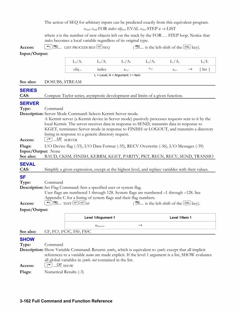
3-162 Full Command and Function Reference
The action of SEQ for arbitrary inputs can be predicted exactly from this equivalent program. xstart xend FOR index objexec EVAL xincr STEP n → LIST
where n is the number of new objects left on the stack by the FOR STEP loop. Notice that index becomes a local variable regardless of its original type.
Access: !° LIST PROCEDURES LSEQ ( °is the left-shift of the Nkey). Input/Output:
L5/A1 L4/A2 L3/A3 L2/A4 L1/A5 Li/I1
objexec index xstart xend xιncr → list L = Level; A = Argument; I = item
See also: DOSUBS, STREAM
SERIES CAS: Compute Taylor series, asymptotic development and limits of a given function.
SERVER Type: Command Description: Server Mode Command: Selects Kermit Server mode. A Kermit server (a Kermit device in Server mode) passively processes requests sent to it by the
local Kermit. The server receives data in response to SEND, transmits data in response to KGET, terminates Server mode in response to FINISH or LOGOUT, and transmits a directory listing in response to a generic directory request.
Access: µ SERVER Flags: I/O Device flag (-33), I/O Data Format (-35), RECV Overwrite (-36), I/O Messages (-39) Input/Output: None See also: BAUD, CKSM, FINISH, KERRM, KGET, PARITY, PKT, RECN, RECV, SEND, TRANSIO
SEVAL CAS: Simplify a given expression, except at the highest level, and replace variables with their values.
SF Type: Command Description: Set Flag Command: Sets a specified user or system flag. User flags are numbered 1 through 128. System flags are numbered 1 through 128. See
Appendix C for a listing of system flags and their flag numbers. Access: !°TEST LLSF ( °is the left-shift of the Nkey). Input/Output:
Level 1/Argument 1 Level 1/Item 1
nflagnumber → See also: CF, FC?, FC?C, FS?, FS?C
SHOW Type: Command Description: Show Variable Command: Returns symb2, which is equivalent to symb1 except that all implicit
references to a variable name are made explicit. If the level 1 argument is a list, SHOW evaluates all global variables in symb1 not contained in the list.
Access: µSHOW Flags: Numerical Results (-3)
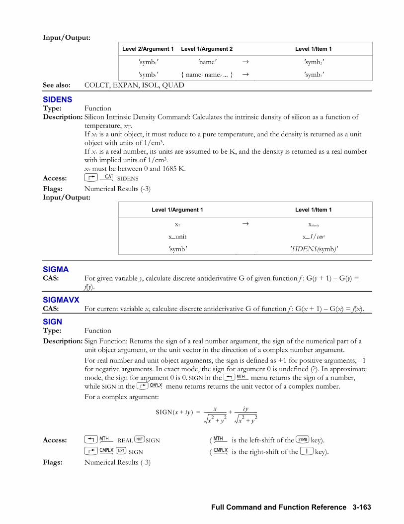
Full Command and Function Reference 3-163
Input/Output: Level 2/Argument 1 Level 1/Argument 2 Level 1/Item 1
'symb1' 'name' → 'symb2'
'symb1' name1 name2 ... → 'symb2' See also: COLCT, EXPAN, ISOL, QUAD
SIDENS Type: Function Description: Silicon Intrinsic Density Command: Calculates the intrinsic density of silicon as a function of
temperature, xT. If xT is a unit object, it must reduce to a pure temperature, and the density is returned as a unit
object with units of 1/cm3. If xT is a real number, its units are assumed to be K, and the density is returned as a real number
with implied units of 1/cm3. xT must be between 0 and 1685 K. Access: µ SIDENS Flags: Numerical Results (-3) Input/Output:
Level 1/Argument 1 Level 1/Item 1
xT → xdensity
x_unit x_1/cm3
'symb' 'SIDENS(symb)'
SIGMA CAS: For given variable y, calculate discrete antiderivative G of given function f : G(y + 1) G(y) =
f(y).
SIGMAVX CAS: For current variable x, calculate discrete antiderivative G of function f : G(x + 1) G(x) = f(x).
SIGN Type: Function Description: Sign Function: Returns the sign of a real number argument, the sign of the numerical part of a
unit object argument, or the unit vector in the direction of a complex number argument. For real number and unit object arguments, the sign is defined as +1 for positive arguments, 1
for negative arguments. In exact mode, the sign for argument 0 is undefined (?). In approximate mode, the sign for argument 0 is 0. SIGN in the !´menu returns the sign of a number, while SIGN in the ß menu returns returns the unit vector of a complex number.
For a complex argument:
SIGN x iy+( ) x
x2 y2+--------------------- iy
x2 y2+---------------------+=
Access: !´ REAL LSIGN ( ´ is the left-shift of the Pkey). ßL SIGN ( ß is the right-shift of the 1key). Flags: Numerical Results (-3)
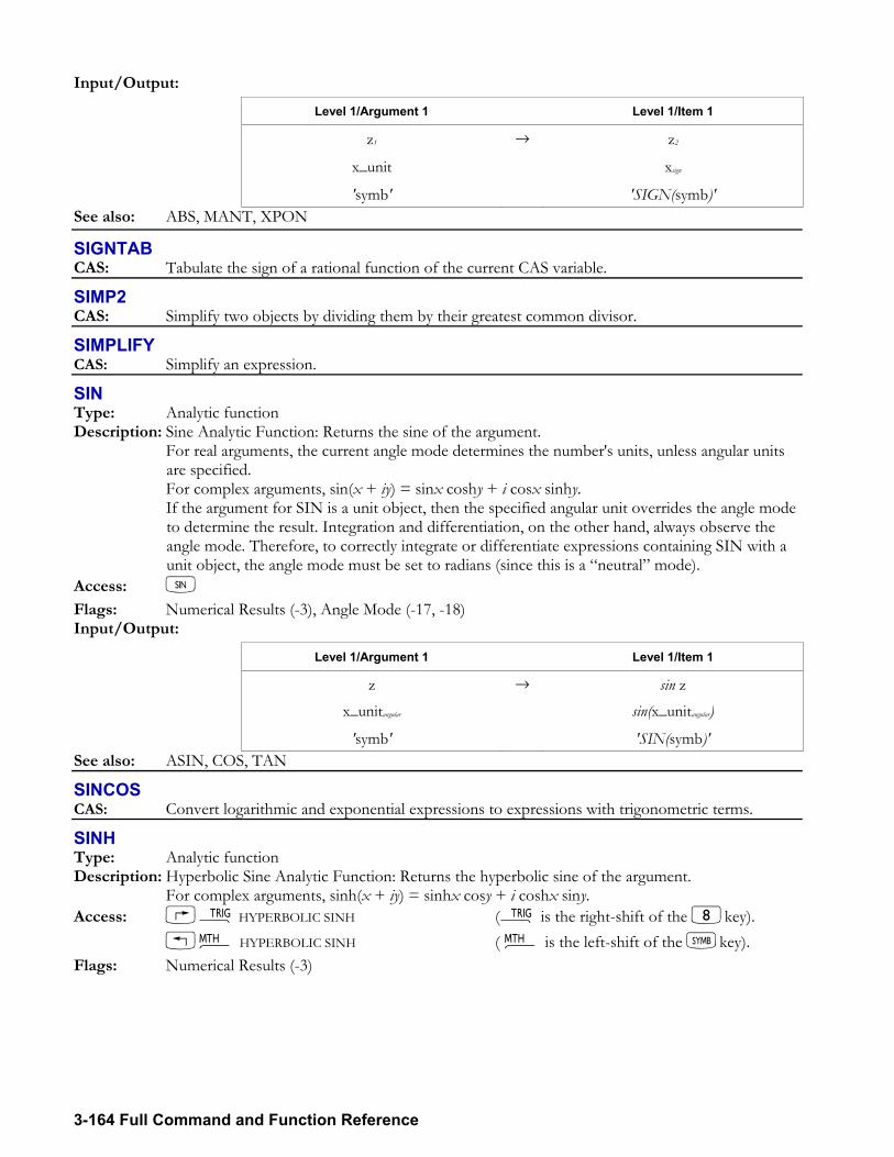
3-164 Full Command and Function Reference
Input/Output: Level 1/Argument 1 Level 1/Item 1
z1 → z2
x_unit xsign
'symb' 'SIGN(symb)' See also: ABS, MANT, XPON
SIGNTAB CAS: Tabulate the sign of a rational function of the current CAS variable.
SIMP2 CAS: Simplify two objects by dividing them by their greatest common divisor.
SIMPLIFY CAS: Simplify an expression.
SIN Type: Analytic function Description: Sine Analytic Function: Returns the sine of the argument. For real arguments, the current angle mode determines the number's units, unless angular units
are specified. For complex arguments, sin(x + iy) = sinx coshy + i cosx sinhy. If the argument for SIN is a unit object, then the specified angular unit overrides the angle mode
to determine the result. Integration and differentiation, on the other hand, always observe the angle mode. Therefore, to correctly integrate or differentiate expressions containing SIN with a unit object, the angle mode must be set to radians (since this is a neutral mode).
Access: S
Flags: Numerical Results (-3), Angle Mode (-17, -18) Input/Output:
Level 1/Argument 1 Level 1/Item 1
z → sin z x_unitangular sin(x_unitangular)
'symb' 'SIN(symb)' See also: ASIN, COS, TAN
SINCOS CAS: Convert logarithmic and exponential expressions to expressions with trigonometric terms.
SINH Type: Analytic function Description: Hyperbolic Sine Analytic Function: Returns the hyperbolic sine of the argument. For complex arguments, sinh(x + iy) = sinhx cosy + i coshx siny. Access: Ñ HYPERBOLIC SINH (Ñ is the right-shift of the 8key). !´ HYPERBOLIC SINH ( ´ is the left-shift of the Pkey). Flags: Numerical Results (-3)
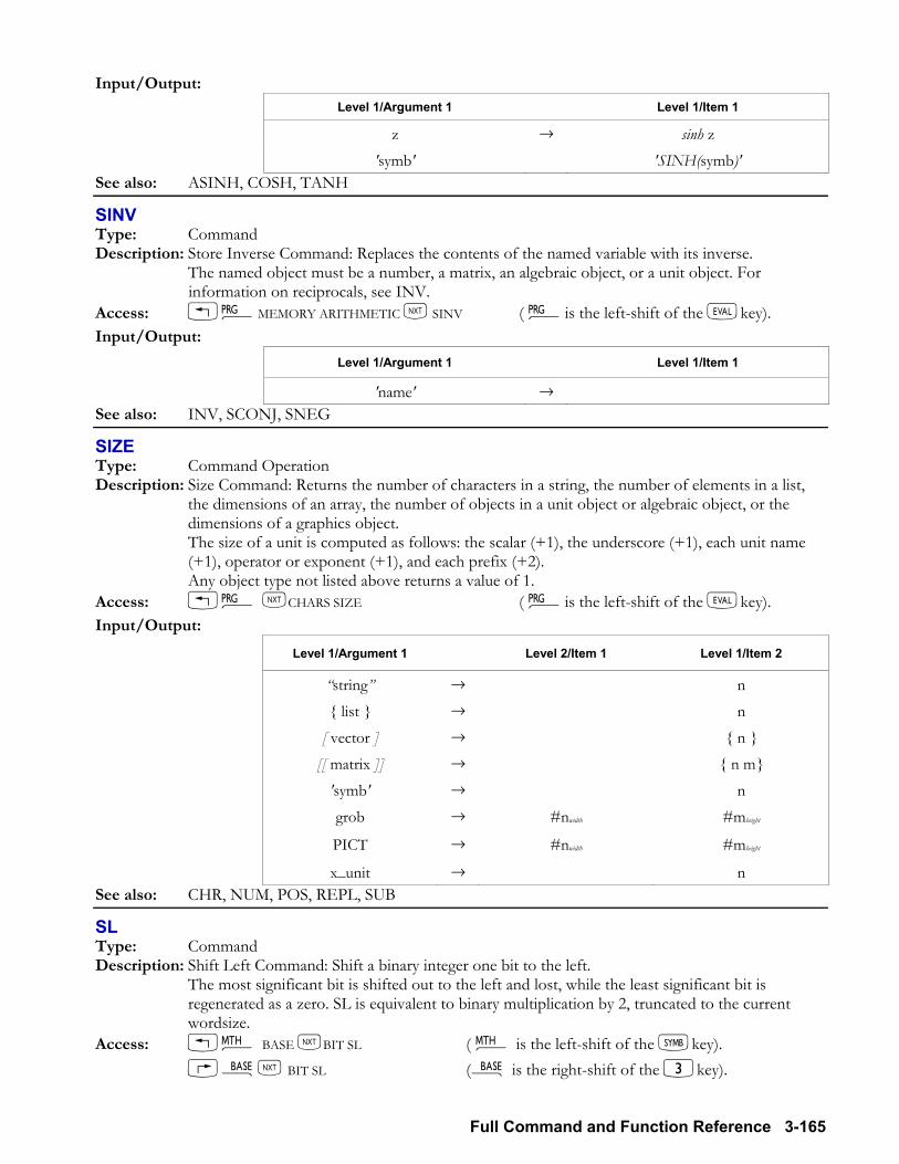
Full Command and Function Reference 3-165
Input/Output: Level 1/Argument 1 Level 1/Item 1
z → sinh z 'symb' 'SINH(symb)'
See also: ASINH, COSH, TANH
SINV Type: Command Description: Store Inverse Command: Replaces the contents of the named variable with its inverse. The named object must be a number, a matrix, an algebraic object, or a unit object. For
information on reciprocals, see INV. Access: !°MEMORY ARITHMETIC L SINV ( °is the left-shift of the Nkey). Input/Output:
Level 1/Argument 1 Level 1/Item 1
'name' → See also: INV, SCONJ, SNEG
SIZE Type: Command Operation Description: Size Command: Returns the number of characters in a string, the number of elements in a list,
the dimensions of an array, the number of objects in a unit object or algebraic object, or the dimensions of a graphics object.
The size of a unit is computed as follows: the scalar (+1), the underscore (+1), each unit name (+1), operator or exponent (+1), and each prefix (+2).
Any object type not listed above returns a value of 1. Access: !° LCHARS SIZE ( °is the left-shift of the Nkey). Input/Output:
Level 1/Argument 1 Level 2/Item 1 Level 1/Item 2
string → n
list → n
[ vector ] → n [[ matrix ]] → n m
'symb' → n
grob → #nwidth #mheight
PICT → #nwidth #mheight
x_unit → n See also: CHR, NUM, POS, REPL, SUB
SL Type: Command Description: Shift Left Command: Shift a binary integer one bit to the left. The most significant bit is shifted out to the left and lost, while the least significant bit is
regenerated as a zero. SL is equivalent to binary multiplication by 2, truncated to the current wordsize.
Access: !´ BASE LBIT SL ( ´ is the left-shift of the Pkey). ãL BIT SL (ã is the right-shift of the 3key).
3-166 Full Command and Function Reference
Flags: Binary Integer Wordsize (-5 through -10), Binary Integer Base (-11, -12) Input/Output:
Level 1/Argument 1 Level 1/Item 1
#n1 → #n2 See also: ASR, SLB, SR, SRB
SLB Type: Command Description: Shift Left Byte Command: Shifts a binary integer one byte to the left. The most significant byte is shifted out to the left and lost, while the least significant byte is
regenerated as zero. SLB is equivalent to binary multiplication by 28 (256) (or executing SL eight times), truncated to the current wordsize.
Access: !´ BASE LBYTE SLB ( ´ is the left-shift of the Pkey). ãL BYTE SLB (ã is the right-shift of the 3key). Flags: Binary Integer Wordsize (-5 through -10), Binary Integer Base (-11, -12) Input/Output:
Level 1/Argument 1 Level 1/Item 1
#n1 → #n2 See also: ASR, SL, SR, SRB
SLOPEFIELD Type: Command Description: SLOPEFIELD Plot Type Command: Sets the plot type to SLOPEFIELD. When plot type is set to SLOPEFIELD, the DRAW command plots a slope representation of a
scalar function with two variables. SLOPEFIELD requires values in the reserved variables EQ, VPAR, and PPAR.
VPAR has the following form: xleft xright ynear yfar zlow zhigh xmin xmax ymin ymax xeye yeye zeye xstep ystep For plot type SLOPEFIELD, the elements of VPAR are used as follows:
xleft and xright are real numbers that specify the width of the view space. ynear and yfar are real numbers that specify the depth of the view space. zlow and zhigh are real numbers that specify the height of the view space. xmin and xmax are not used. ymin and ymax are not used. xeye, yeye, and zeye are real numbers that specify the point in space from which the graph is
viewed. xstep and ystep are real numbers that set the number of x-coordinates versus the number of y-
coordinates plotted. The plotting parameters are specified in the reserved variable PPAR, which has this form:
(xmin, ymin) (xmax, ymax) indep res axes ptype depend For plot type SLOPEFIELD, the elements of PPAR are used as follows:
(xmin, ymin) is not used. (xmax, ymax) is not used. indep is a name specifying the independent variable. The default value of indep is X. res is not used. axes is not used. ptype is a command name specifying the plot type. Executing the command SLOPEFIELD
places the command name SLOPEFIELD in ptype. depend is a name specifying the dependent variable. The default value is Y.
Full Command and Function Reference 3-167
Access: µ SLOPEFIELD Input/Output: None See also: BAR, CONIC, DIFFEQ, FUNCTION, GRIDMAP, HISTOGRAM, PARAMETRIC,
PARSURFACE, PCONTOUR, POLAR, SCATTER, TRUTH, WIREFRAME, YSLICE
SNEG Type: Command Description: Store Negate Command: Replaces the contents of a variable with its negative. The named object must be a number, an array, an algebraic object, a unit object, or a graphics
object. For information on negation, see NEG. Access: !°MEMORY ARITHMETIC L SNEG ( °is the left-shift of the Nkey). Input/Output:
Level 1/Argument 1 Level 1/Item 1
'name' →
See also: NEG, SCONJ, SINV
SNRM Type: Command Description: Spectral Norm Command: Returns the spectral norm of an array. The spectral norm of a vector is its Euclidean length, and is equal to the largest singular value of
a matrix. Access: !Ø OPERATIONS L L SNRM ( Ø is the left-shift of the 5key). !´ MATRIX NORMALIZE SNRM ( ´ is the left-shift of the Pkey). Input/Output:
Level 1/Argument 1 Level 1/Item 1
[ array ] → xspectralnorm See also: ABS, CNRM, COND, RNRM, SRAD, TRACE
SOLVE CAS: Find zeros of an expression, or solve an equation with respect to a specified variable.
SOLVEQN Type: Command Description: Starts the appropriate solver for a specified set of equations. SOLVEQN sets up and starts the appropriate solver for the specified set of equations, bypassing
the Equation Library catalogs. It sets EQ (and Mpar if more than one equation is being solved), sets the unit options according to flags -60 and -61, and starts the appropriate solver.
SOLVEQN uses subject and title numbers (levels 3 and 2) and a PICT option (level 1) and returns nothing. Subject and title numbers are listed in chapter 5. For example, a 2 in level 3 and a 9 in level 2 would specify the Electricity category and Capacitive Energy set of equations. If the PICT option is 0, PICT is not affected; otherwise, the equation picture (if any) is copied into PICT.
Access: µ SOLVEQN Flags: Unit Type (-60), Units Usage (-61) Input/Output:
Level 3/Argument 1 Level 2/Argument 2 Level 1/Argument 3 Level 1/Item 1
n m 0/1 → See also: EQNLIB, MSOLVER
3-168 Full Command and Function Reference
SOLVER Type: Command Description: Displays a menu of commands used in solving equations. Access: µ SOLVER Input/Output: None
SOLVEVX CAS: Find zeros of an expression, or solves an equation with respect to the current variable.
SORT Type: Command Description: Ascending Order Sort Command: Sorts the elements in a list in ascending order. The elements in the list can be real numbers, strings, lists, names, binary integers, or unit objects.
However, all elements in the list must all be of the same type. Strings and names are sorted by character code number. Lists of lists are sorted by the first element in each list.
To sort in reverse order, use SORT REVLIST. Access: !´ LIST SORT ( ´ is the left-shift of the Pkey). !° LIST PROCEDURES L SORT ( °is the left-shift of the Nkey). Input/Output:
Level 1/Argument 1 Level 1/Item 1
list 1 → list 2 See also: REVLIST
SPHERE Type: Command Description: Spherical Mode Command: Sets spherical coordinate mode. SPHERE sets flags 15 and 16. In spherical mode, vectors are displayed as polar components. Access: &H ANGLE SPHERE Input/Output: None See also: CYLIN, RECT
SQ Type: Analytic function Description: Square Analytic Function: Returns the square of the argument. The square of a complex argument (x, y) is the complex number (x2 y2, 2xy). Matrix arguments must be square. Access: !º ( º is the left-shift of the Rkey). Flags: Numerical Results (-3) Input/Output:
Level 1/Argument 1 Level 1/Item 1
z → z2
x_unit → x2_unit2
[[ matrix ]] → [[ matrix × matrix ]]
'symb' → 'SQ(symb)' See also: √, ^
Full Command and Function Reference 3-169
SR Type: Command Description: Shift Right Command: Shifts a binary integer one bit to the right. The least significant bit is shifted out to the right and lost, while the most significant bit is
regenerated as a zero. SR is equivalent to binary division by 2. Access: !´ BASE L BIT SR ( ´ is the left-shift of the Pkey). ã L BIT SR (ã is the right-shift of the 3key). Flags: Binary Integer Wordsize (-5 through -10), Binary Integer Base (-11, -12) Input/Output:
Level 1/Argument 1 Level 1/Item 1
#n1 → #n2 See also: ASR, SL, SLB, SRB
SRAD Type: Command Description: Spectral Radius Command: Returns the spectral radius of a square matrix. The spectral radius of a matrix is a measure of the size of the matrix, and is equal to the absolute
value of the largest eigenvalue of the matrix. Access: !Ø OPERATIONS L L SRAD (Ø is the left-shift of the 5key). !´ MATRIX NORMALIZE SRAD ( ´ is the left-shift of the Pkey). Input/Output:
Level 1/Argument 1 Level 1/Item 1
[[ matrix ]]n×n → xspectralradius See also: COND, SNRM, TRACE
SRB Type: Command Description: Shift Right Byte Command: Shifts a binary integer one byte to the right. The least significant byte is shifted out to the right and lost, while the most significant byte is
regenerated as zero. SRB is equivalent to binary division by 28 (or executing SR eight times). Access: !´ BASE L BYTE SRB ( ´ is the left-shift of the Pkey). ã L BYTE SRB (ã is the right-shift of the 3key). Flags: Binary Integer Wordsize (-5 through -10), Binary Integer Base (-11, -12) Input/Output:
Level 1/Argument 1 Level 1/Item 1
#n1 → #n2 See also: ASR, SL, SLB, SR
SRECV Type: Command Description: Serial Receive Command: Reads up to n characters from the serial input buffer and returns them
as a string, along with a digit indicating whether errors occurred. SRECV does not use Kermit protocol. If n characters are not received within the time specified by STIME (default is 10 seconds),
SRECV times out, returning a 0 to level 1 and as many characters as were received to level 2.
3-170 Full Command and Function Reference
If the level 2 output from BUFLEN is used as the input for SRECV, SRECV will not have to wait for more characters to be received. Instead, it returns the characters already in the input buffer.
If you want to accumulate bytes in the input buffer before executing SRECV, you must first open the port using OPENIO (if the port isn't already open).
SRECV can detect three types of error when reading the input buffer: Framing errors and UART overruns (both causing "Receive Error" in ERRM). Input-buffer overflows (causing "Receive Buffer Overflow" in ERRM). Parity errors (causing "Parity Error" in ERRM).
SRECV returns 0 if an error is detected when reading the input buffer, or 1 if no error is detected.
Parity errors do not stop data flow into the input buffer. However, if a parity error occurs, SRECV stops reading data after encountering a character with an error.
Framing, overrun, and overflow errors cause all subsequently received characters to be ignored until the error is cleared. SRECV does not detect and clear any of these types of errors until it tries to read the byte where the error occurred. Since these three errors cause the byte where the error occurred and all subsequent bytes to be ignored, the input buffer will be empty after all previously received good bytes have been read. Therefore, SRECV detects and clears these errors when it tries to read a byte from an empty input buffer.
Note that BUFLEN also clears the above-mentioned framing, overrun, and overflow errors. Therefore, SRECV cannot detect an input-buffer overflow after BUFLEN is executed, unless more characters were received after BUFLEN was executed (causing the input buffer to overflow again). SRECV also cannot detect framing and UART overrun errors cleared by BUFLEN. To find where the data error occurred, save the number of characters returned by BUFLEN (which gives the number of good characters received), because as soon as the error is cleared, new characters can enter the input buffer.
Access: µSRECV Flags: I/O Device (-33) Input/Output:
Level 1/Argument 1 Level 2/Item 1 Level 1/Item 2
n → 'string' 0/1 See also: BUFLEN, CLOSEIO, OPENIO, SBRK, STIME, XMIT
SREPL Type: Command Description: Find and replace: Finds and replaces a string in a given text object. You supply the following
inputs: Level 3/argument 1: the string to search. Level 2/argument 2: the string to find. Level 1/argument 3: the string to replace it with.
Access: &NLSREPL °LCHARS LSREPL ( °is the left-shift of the Nkey). Input/Output:
Level 3/Argument 1 Level 2/Argument 2 Level 1/Argument 3 Level 1/Item 1
'string' 'string' 'string' → 'string' See also: REPL
START Type: Command Operation
Full Command and Function Reference 3-171
Description: START Definite Loop Structure Command: Begins START NEXT and START STEP definite loop structures.
Definite loop structures execute a command or sequence of commands a specified number of times. START NEXT executes a portion of a program a specified number of times. The RPL syntax is this: xstart xfinish START loop-clause NEXT
The algebraic syntax is this: START(xstart xfinish) loop-clause NEXT START takes two numbers (xstart and xfinish) from the stack and stores them as the starting and ending values for a loop counter. Then the loop clause is executed. NEXT increments the counter by 1 and tests to see if its value is less than or equal to xfinish. If so, the loop clause is executed again. Notice that the loop clause is always executed at least once.
START STEP works just like START NEXT, except that it can use an increment value other than 1. The RPL syntax is this: xstart xfinish START loop-clause xincrement STEP The algebraic syntax is this: START (xstart xfinish ) loop-clause STEP(xincrement) START takes two numbers (xstart and xfinish) from the stack and stores them as the starting and ending values for the loop counter. Then the loop clause is executed. STEP takes xincrement from the stack and increments the counter by that value. If the argument of STEP is an algebraic or a name, it is automatically evaluated to a number. The increment value can be positive or negative: If positive, the loop is executed again when the counter is less than or equal to xfinish. If negative, the loop is executed when the counter is greater than or equal to xfinish.
Access: !°BRANCH START ( °is the left-shift of the Nkey). Input/Output:
Level 2/Argument 1 Level 1/Argument 2 Level 1/Item 1
START xstart xfinish →
NEXT → STEP xincrement →
STEP 'symbincrement' → See also: FOR, NEXT, STEP
STD Type: Command Description: Standard Mode Command: Sets the number display format to standard mode. Executing STD has the same effect as clearing flags 49 and 50. Standard format produces the following results when displaying or printing a number.
Numbers that can be represented exactly as integers with 12 or fewer digits are displayed without a fraction mark or exponent. Zero is displayed as 0.
Numbers that can be represented exactly with 12 or fewer digits, but not as integers, are displayed with a fraction mark but no exponent. Leading zeros to the left of the fraction mark and trailing zeros to the right of the fraction mark are omitted.
All other numbers are displayed in scientific notation (see SCI) with both a fraction mark (with one number to the left) and an exponent (of one or three digits). There are no leading or trailing zeros.
In algebraic objects, integers less than 103 are always displayed in standard mode. Access: µ STD Input/Output: None See also: ENG, FIX, SCI
3-172 Full Command and Function Reference
STEP Type: Command Operation Description: STEP Command: Defines the increment (step) value, and ends definite loop structure. See the FOR and START keyword entries for more information. Access: !°BRANCH START/FOR STEP ( °is the left-shift of the Nkey). Input/Output: None See also: FOR, NEXT, START
STEQ Type: Command Description: Store in EQ Command: Stores an object into the reserved variable EQ in the current directory. Access: µ STEQ Input/Output:
Level 1/Argument 1 Level 1/Item 1
obj → See also: RCEQ
STIME Type: Command Description: Serial Time-Out Command: Specifies the period that SRECV (serial reception) and XMIT (serial
transmission) wait before timing out. The value for x is interpreted as a positive value from 0 to 25.4 seconds. If no value is given, the
default is 10 seconds. If x is 0, there is no time-out; that is, the device waits indefinitely, which can drain the batteries.
STIME is not used for Kermit time-out. Access: µ STIME Input/Output:
Level 1/Argument 1 Level 1/Item 1
xseconds →
0 → See also: BUFLEN, CLOSEIO, SBRK, SRECV, XMIT
STO Type: Command Description: Store Command: Stores an object into a specified variable or object. Storing a graphics object into PICT makes it the current graphics object. To create a backup object, store the obj into the desired backup location (identified as
:nport:namebackup). STO will not overwrite an existing backup object. To store backup objects and library objects, specify a port number (0 through 3). After storing a library object in a port, it must then be attached to its directory before it can be used.
The easiest way to do this is to execute a warm start (by pressing $& C). This also causes the calculator to perform a system halt, which clears the stack, the LAST stack, and all local variables.
STO can also replace a single element of an array or list stored in a variable. Specify the variable in level 1 as name(index), which is a user function with index as the argument. The index can be n or n,m, where n specifies the row position in a vector or list, and n,m specifies the row-and-column position in a matrix.
Access: K
Full Command and Function Reference 3-173
Input/Output: Level 2/Argument 1 Level 1/Argument 2 Level 1/Item 1
obj 'name' → grob PICT → obj :nport :namebackup →
obj 'name(index)' → backup nport →
library nport →
library :nport :nlibrary → See also: DEFINE, RCL, →, !
STOALARM Type: Command Description: Store Alarm Command: Stores an alarm in the system alarm list and returns its alarm index
number. If the argument is a real number xtime, the alarm date will be the current system date by default. If objaction is a string, the alarm is an appointment alarm, and the string is the alarm message. If
objaction is any other object type, the alarm is a control alarm, and the object is executed when the alarm comes due.
xrepeat is the repeat interval for the alarm in clock ticks, where 8192 ticks equals 1 second. nindex is a real integer identifying the alarm based on its chronological position in the system alarm
list. Access: ÓTOOLS ALRM STOALARM (Ó is the right-shift of the 9 key). Flags: Date Format (-42), Repeat Alarms Not Rescheduled (-43), Acknowledged Alarms Saved (-44) Input/Output:
Level 1/Argument 1 Level 1/Item 1
xtime → nindex date time → nindex
date time objaction → nindex date time objaction xrepeat → nindex
See also: DELALARM, FINDALARM, RCLALARM
STOF Type: Command Description: Store Flags Command: Sets the states of the system flags or the system and user flags. With argument #nsystem, STOF sets the states of the system flags (1 through 128) only. With
argument #nsystem, #nuser, #nsystem2 #nuser2 , STOF sets the states of both the system and user flags. A bit with value 1 sets the corresponding flag; a bit with value 0 clears the corresponding flag.
The rightmost (least significant) bit of #nsystem and #nuser correspond to the states of system flag 1 and user flag +1, respectively.
STOF can preserve the states of flags before a program executes and changes the states. RCLF can then recall the flag's states after the program is executed.
Access: µ STOF Flags: Binary Integer Wordsize (-5 through -10)
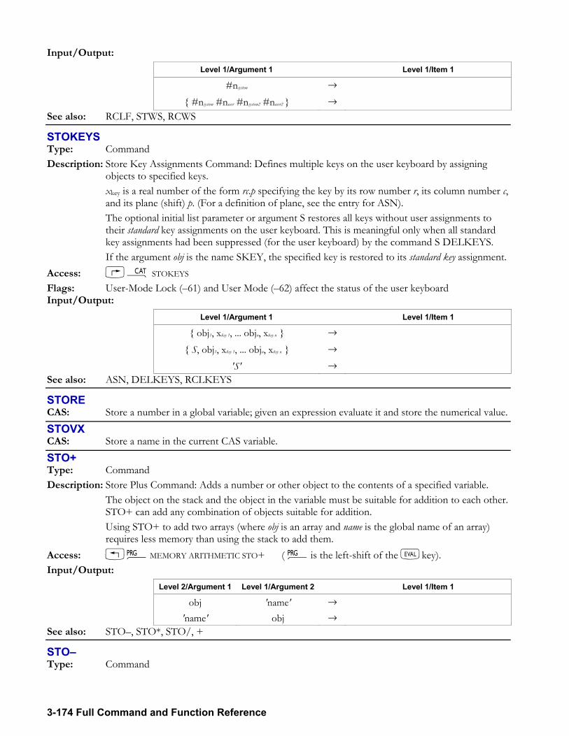
3-174 Full Command and Function Reference
Input/Output: Level 1/Argument 1 Level 1/Item 1
#nsystem →
#nsystem #nuser #nsystem2 #nuser2 →
See also: RCLF, STWS, RCWS
STOKEYS Type: Command Description: Store Key Assignments Command: Defines multiple keys on the user keyboard by assigning
objects to specified keys. xkey is a real number of the form rc.p specifying the key by its row number r, its column number c,
and its plane (shift) p. (For a definition of plane, see the entry for ASN). The optional initial list parameter or argument S restores all keys without user assignments to
their standard key assignments on the user keyboard. This is meaningful only when all standard key assignments had been suppressed (for the user keyboard) by the command S DELKEYS.
If the argument obj is the name SKEY, the specified key is restored to its standard key assignment. Access: µ STOKEYS Flags: User-Mode Lock (61) and User Mode (62) affect the status of the user keyboard Input/Output:
Level 1/Argument 1 Level 1/Item 1
obj1, xkey 1, ... objn, xkey n →
S, obj1, xkey 1, ... objn, xkey n →
'S' → See also: ASN, DELKEYS, RCLKEYS
STORE CAS: Store a number in a global variable; given an expression evaluate it and store the numerical value.
STOVX CAS: Store a name in the current CAS variable.
STO+ Type: Command Description: Store Plus Command: Adds a number or other object to the contents of a specified variable. The object on the stack and the object in the variable must be suitable for addition to each other.
STO+ can add any combination of objects suitable for addition. Using STO+ to add two arrays (where obj is an array and name is the global name of an array)
requires less memory than using the stack to add them. Access: !°MEMORY ARITHMETIC STO+ ( °is the left-shift of the Nkey). Input/Output:
Level 2/Argument 1 Level 1/Argument 2 Level 1/Item 1
obj 'name' → 'name' obj →
See also: STO, STO*, STO/, +
STO Type: Command
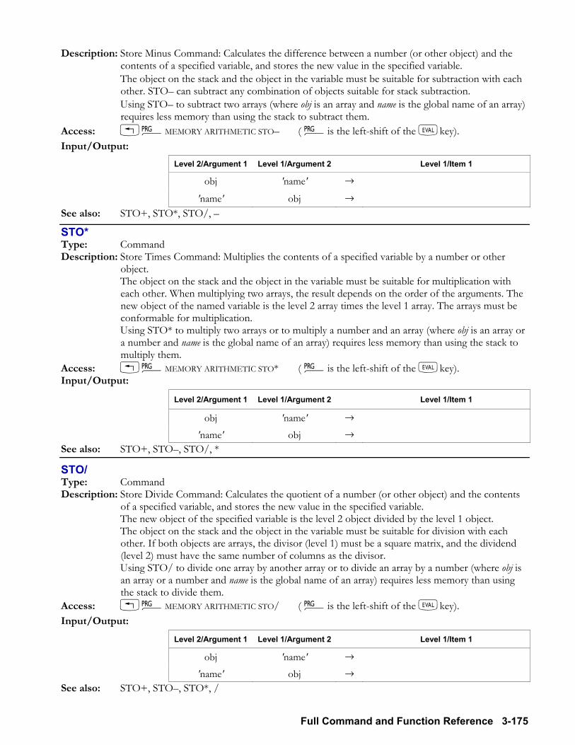
Full Command and Function Reference 3-175
Description: Store Minus Command: Calculates the difference between a number (or other object) and the contents of a specified variable, and stores the new value in the specified variable.
The object on the stack and the object in the variable must be suitable for subtraction with each other. STO can subtract any combination of objects suitable for stack subtraction.
Using STO to subtract two arrays (where obj is an array and name is the global name of an array) requires less memory than using the stack to subtract them.
Access: !°MEMORY ARITHMETIC STO ( °is the left-shift of the Nkey). Input/Output:
Level 2/Argument 1 Level 1/Argument 2 Level 1/Item 1
obj 'name' →
'name' obj → See also: STO+, STO*, STO/,
STO* Type: Command Description: Store Times Command: Multiplies the contents of a specified variable by a number or other
object. The object on the stack and the object in the variable must be suitable for multiplication with
each other. When multiplying two arrays, the result depends on the order of the arguments. The new object of the named variable is the level 2 array times the level 1 array. The arrays must be conformable for multiplication.
Using STO* to multiply two arrays or to multiply a number and an array (where obj is an array or a number and name is the global name of an array) requires less memory than using the stack to multiply them.
Access: !°MEMORY ARITHMETIC STO* ( °is the left-shift of the Nkey). Input/Output:
Level 2/Argument 1 Level 1/Argument 2 Level 1/Item 1
obj 'name' → 'name' obj →
See also: STO+, STO, STO/, *
STO/ Type: Command Description: Store Divide Command: Calculates the quotient of a number (or other object) and the contents
of a specified variable, and stores the new value in the specified variable. The new object of the specified variable is the level 2 object divided by the level 1 object. The object on the stack and the object in the variable must be suitable for division with each
other. If both objects are arrays, the divisor (level 1) must be a square matrix, and the dividend (level 2) must have the same number of columns as the divisor.
Using STO/ to divide one array by another array or to divide an array by a number (where obj is an array or a number and name is the global name of an array) requires less memory than using the stack to divide them.
Access: !°MEMORY ARITHMETIC STO/ ( °is the left-shift of the Nkey). Input/Output:
Level 2/Argument 1 Level 1/Argument 2 Level 1/Item 1
obj 'name' → 'name' obj →
See also: STO+, STO, STO*, /
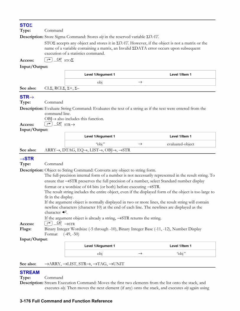
3-176 Full Command and Function Reference
STOΣ Type: Command Description: Store Sigma Command: Stores obj in the reserved variable ΣDAT. STOΣ accepts any object and stores it in ΣDAT. However, if the object is not a matrix or the
name of a variable containing a matrix, an Invalid ΣDATA error occurs upon subsequent execution of a statistics command.
Access: µ STOΣ Input/Output:
Level 1/Argument 1 Level 1/Item 1
obj → See also: CLΣ, RCLΣ, Σ+, Σ
STR→ Type: Command Description: Evaluate String Command: Evaluates the text of a string as if the text were entered from the
command line. OBJ→ also includes this function. Access: µ STR→ Input/Output:
Level 1/Argument 1 Level 1/Item 1
obj → evaluated-object See also: ARRY→, DTAG, EQ→, LIST→, OBJ→, →STR
→STR Type: Command Description: Object to String Command: Converts any object to string form. The full-precision internal form of a number is not necessarily represented in the result string. To
ensure that →STR preserves the full precision of a number, select Standard number display format or a wordsize of 64 bits (or both) before executing →STR.
The result string includes the entire object, even if the displayed form of the object is too large to fit in the display.
If the argument object is normally displayed in two or more lines, the result string will contain newline characters (character 10) at the end of each line. The newlines are displayed as the character .
If the argument object is already a string, →STR returns the string. Access: µ →STR Flags: Binary Integer Wordsize (-5 through -10), Binary Integer Base (-11, -12), Number Display
Format (-49, -50) Input/Output:
Level 1/Argument 1 Level 1/Item 1
obj → obj
See also: →ARRY, →LIST, STR→, →TAG, →UNIT
STREAM Type: Command Description: Stream Execution Command: Moves the first two elements from the list onto the stack, and
executes obj. Then moves the next element (if any) onto the stack, and executes obj again using
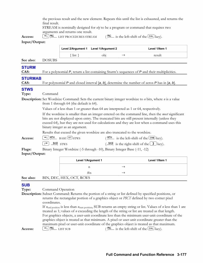
Full Command and Function Reference 3-177
the previous result and the new element. Repeats this until the list is exhausted, and returns the final result.
STREAM is nominally designed for obj to be a program or command that requires two arguments and returns one result.
Access: !°LIST PROCEDURES STREAM ( °is the left-shift of the Nkey). Input/Output:
Level 2/Argument 1 Level 1/Argument 2 Level 1/Item 1
list obj → result See also: DOSUBS
STURM CAS: For a polynomial P, return a list containing Sturms sequences of P and their multiplicities.
STURMAB CAS: For polynomial P and closed interval [a, b], determine the number of zeros P has in [a, b].
STWS Type: Command Description: Set Wordsize Command: Sets the current binary integer wordsize to n bits, where n is a value
from 1 through 64 (the default is 64). Values of n less than 1 or greater than 64 are interpreted as 1 or 64, respectively. If the wordsize is smaller than an integer entered on the command line, then the most significant
bits are not displayed upon entry. The truncated bits are still present internally (unless they exceed 64), but they are not used for calculations and they are lost when a command uses this binary integer as an argument.
Results that exceed the given wordsize are also truncated to the wordsize. Access: !´ BASE LSTWS ( ´ is the left-shift of the Pkey). ã STWS (ã is the right-shift of the 3key). Flags: Binary Integer Wordsize (-5 through -10), Binary Integer Base (-11, -12) Input/Output:
Level 1/Argument 1 Level 1/Item 1
n → #n →
See also: BIN, DEC, HEX, OCT, RCWS
SUB Type: Command Operation Description: Subset Command: Returns the portion of a string or list defined by specified positions, or
returns the rectangular portion of a graphics object or PICT defined by two corner pixel coordinates.
If nend position is less than nstart position, SUB returns an empty string or list. Values of n less than 1 are treated as 1; values of n exceeding the length of the string or list are treated as that length.
For graphics objects, a user-unit coordinate less than the minimum user-unit coordinate of the graphics object is treated as that minimum. A pixel or user-unit coordinate greater than the maximum pixel or user-unit coordinate of the graphics object is treated as that maximum.
Access: !°LIST SUB ( °is the left-shift of the Nkey).
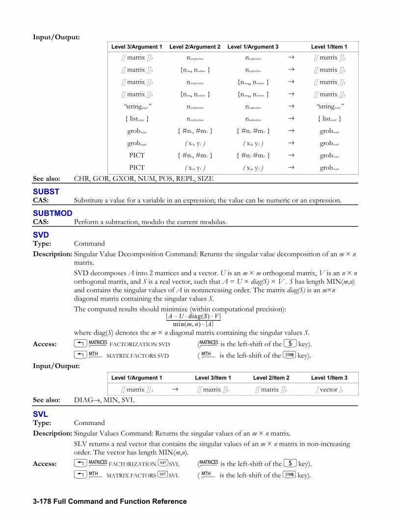
3-178 Full Command and Function Reference
Input/Output: Level 3/Argument 1 Level 2/Argument 2 Level 1/Argument 3 Level 1/Item 1
[[ matrix ]]1 nstartposition nendposition → [[ matrix ]]2
[[ matrix ]]1 nrow, ncolumn nendposition → [[ matrix ]]2
[[ matrix ]]1 nstartposition nrow,, ncolumn → [[ matrix ]]2
[[ matrix ]]1 nrow, ncolumn nrow,, ncolumn → [[ matrix ]]2
stringtarget nstartposition nendposition → stringresult
listtarget nstartposition nendposition → listresult
grobtarget #n1, #m1 #n2 #m2 → grobresult
grobtarget ( x1, y1 ) ( x2, y2 ) → grobresult
PICT #n1, #m1 #n2 #m2 → grobresult
PICT ( x1, y1 ) ( x2, y2 ) → grobresult See also: CHR, GOR, GXOR, NUM, POS, REPL, SIZE
SUBST CAS: Substitute a value for a variable in an expression; the value can be numeric or an expression.
SUBTMOD CAS: Perform a subtraction, modulo the current modulus.
SVD Type: Command Description: Singular Value Decomposition Command: Returns the singular value decomposition of an m × n
matrix. SVD decomposes A into 2 matrices and a vector. U is an m × m orthogonal matrix, V is an n × n
orthogonal matrix, and S is a real vector, such that A = U × diag(S) × V . S has length MIN(m,n) and contains the singular values of A in nonincreasing order. The matrix diag(S) is an m×n diagonal matrix containing the singular values S.
The computed results should minimize (within computational precision): A U diag S( ) V⋅ ⋅
min m n,( ) A⋅---------------------------------------------------
where diag(S) denotes the m × n diagonal matrix containing the singular values S. Access: !Ø FACTORIZATION SVD (Ø is the left-shift of the 5key). !´ MATRIX FACTORS SVD ( ´ is the left-shift of the Pkey). Input/Output:
Level 1/Argument 1 Level 3/Item 1 Level 2/Item 2 Level 1/Item 3
[[ matrix ]]A → [[ matrix ]]U [[ matrix ]]V [ vector ]S See also: DIAG→, MIN, SVL
SVL Type: Command Description: Singular Values Command: Returns the singular values of an m × n matrix. SLV returns a real vector that contains the singular values of an m × n matrix in non-increasing
order. The vector has length MIN(m,n). Access: !Ø FACTORIZATION LSVL (Ø is the left-shift of the 5key). !´ MATRIX FACTORS LSVL ( ´ is the left-shift of the Pkey).
Full Command and Function Reference 3-179
Input/Output: Level 1/Argument 1 Level 1/Item 1
[[ matrix ]] → [ vector ] See also: MIN, SVD
SWAP Type: RPL Command Description: Swap Objects Command: Swaps the position of the two inputs. Access: !°STACK SWAP ( °is the left-shift of the Nkey). in RPN mode executes SWAP when no command line is present. Input/Output:
Level 2 Level 1 Level 2 Level 1
obj1 obj2 → obj2 obj1 See also: DUP, DUPN, DUP2, OVER, PICK, ROLL, ROLLD, ROT
SYSEVAL Type: Command Description: Evaluate System Object Command: Evaluates unnamed operating system objects specified by
their memory addresses.
WARNING: Use extreme care when executing this function. Using SYSEVAL with random addresses will almost always cause a memory loss. Do not use this function unless you know what you are doing.
Access: µ SYSEVAL Input/Output:
Level 1/Argument 1 Level 1/Item 1
#naddress → See also: EVAL, LIBEVAL, FLASHEVAL
SYLVESTER CAS: For symmetric matrix A, return D and P where D is diagonal and A = PTDP.
SYST2MAT CAS: Convert a system of linear equations in algebraic form to matrix form.
%T Type: Function Description: Percent of Total Function: Returns the percent of the first argument that is represented by the
second argument. If both arguments are unit objects, the units must be consistent with each other. The dimensions of a unit object are dropped from the result, but units are part of the calculation. For more information on using temperature units with arithmetic functions, refer to the entry for
+. Access: !´ REAL %T ( ´ is the left-shift of the Pkey). Flags: Numerical Results (-3)
3-180 Full Command and Function Reference
Input/Output: Level 2/Argument 1 Level 1/Argument 2 Level 1/Item 1
x y → 100y/x x 'symb' → '%T(x,symb)'
'symb' x → '%T(symb,x)' 'symb1' 'symb2' → '%T(symb1, symb2)'
x_unit1 y_unit2 → 100y_unit2/x_unit1
x_unit 'symb' → '%T(x_unit,symb)' 'symb' x_unit → '%T(symb,x_unit)'
See also: +, %, %CH
TABVAL CAS: Store given expression, and return results of substituting given values in the expression.
TABVAR CAS: Compute variation table for a function, of the current variable, with a rational derivative.
→TAG Type: Command Description: Stack to Tag Command: Combines objects in levels 1 and 2 to create tagged (labeled) object. The tag argument is a string of fewer than 256 characters. Access: °TYPE →TAG ( °is the left-shift of the Nkey). Input/Output:
Level 2/Argument 1 Level 1/Argument 2 Level 1/Item 1
obj tag → :tag:obj obj 'name' → :name:obj obj x → :x:obj
See also: →ARRY, DTAG, →LIST, OBJ→, →STR, →UNIT
TAIL Type: Command Description: Last Listed Elements Command: Returns all but the first element of a list or string. Access: !°LCHARS LTAIL ( °is the left-shift of the Nkey). Input/Output:
Level 1/Argument 1 Level 1/Item 1
obj1 ... objn → obj2 ... objn
string1 → string2 See also: HEAD
TAN Type: Analytic function Description: Tangent Analytic Function: Returns the tangent of the argument. For real arguments, the current angle mode determines the number's interpretation as an angle,
unless the angular units are specified.
Full Command and Function Reference 3-181
For a real argument that is an odd-integer multiple of 90 in Degrees mode, an Infinite Result exception occurs. If flag 22 is set (no error), the sign of the result (MAXR) matches that of the argument.
For complex arguments: x iy+( )tan xsin( ) xcos( ) i ysinh( ) ycosh( )+
hsin 2y cos2x+-------------------------------------------------------------------------------=
If the argument for TAN is a unit object, then the specified angular unit overrides the angle
mode to determine the result. Integration and differentiation, on the other hand, always observe the angle mode. Therefore, to correctly integrate or differentiate expressions containing TAN with a unit object, the angle mode must be set to Radians (since this is a neutral mode).
Access: U
Flags: Numerical Results (-3), Angle Mode (-17, -18), Inifinite Result Exception (-22) Input/Output:
Level 1/Argument 1 Level 1/Item 1
z → tan z 'symb' → 'TAN(symb)'
x_unitangular tan (x_unitangular) See also: ATAN, COS, SIN
TAN2CS2 CAS: Replace tan(x) terms in expressions with (1-cos(2x))/sin(2x) terms.
TAN2SC CAS: Replace tan(x) terms in expressions with sin(x)/cos(x).
TAN2SC2 CAS: Replace tan(x) terms in expressions with sin(2x)/1+cos(2x) terms.
TANH Type: Analytic function Description: Hyperbolic Tangent Analytic Function: Returns the hyperbolic tangent of the argument. For complex arguments,
x iy+( )tanh 2xsinh i 2ysin+2xcosh 2ycos+---------------------------------------=
Access: Ñ HYPERBOLIC TANH (Ñ is the right-shift of the 8key). !´ HYPERBOLIC TANH ( ´ is the left-shift of the Pkey). Flags: Numerical Results (-3) Input/Output:
Level 1/Argument 1 Level 1/Item 1
z → tanh z 'symb' → 'TANH(symb)'
See also: ATANH, COSH, SINH
TAYLOR0 CAS: Perform a fourth-order Taylor expansion of an expression at x = 0.
TAYLR Type: Command Description: Taylor Polynomial Command: Calculates the nth order Taylor polynomial of symb in the variable
global.
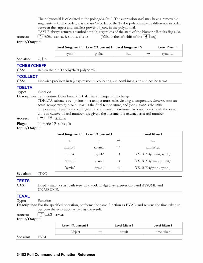
3-182 Full Command and Function Reference
The polynomial is calculated at the point global = 0. The expression symb may have a removable singularity at 0. The order, n, is the relative order of the Taylor polynomialthe difference in order between the largest and smallest power of global in the polynomial.
TAYLR always returns a symbolic result, regardless of the state of the Numeric Results flag (3). Access: !Ö LIMITS & SERIES TAYLR ( Öis the left-shift of the 4key). Input/Output:
Level 3/Argument 1 Level 2/Argument 2 Level 1/Argument 3 Level 1/Item 1
'symb' 'global' norder → 'symbTaylor' See also: ∂, ∫, Σ
TCHEBYCHEFF CAS: Return the nth Tchebycheff polynomial.
TCOLLECT CAS: Linearize products in trig expression by collecting and combining sine and cosine terms.
TDELTA Type: Function Description: Temperature Delta Function: Calculates a temperature change. TDELTA subtracts two points on a temperature scale, yielding a temperature increment (not an
actual temperature). x or x_unit1 is the final temperature, and y or y_unit2 is the initial temperature. If unit objects are given, the increment is returned as a unit object with the same units as x_unit1. If real numbers are given, the increment is returned as a real number.
Access: µ TDELTA Flags: Numerical Results (-3) Input/Output:
Level 2/Argument 1 Level 1/Argument 2 Level 1/Item 1
x y → xdelta
x_unit1 x_unit2 → x_unit1delta
x_unit 'symb' → 'TDELTA(x_unit, symb)'
'symb' y_unit → 'TDELTA(symb, y_unit)'
'symb1' 'symb2' → 'TDELTA(symb1, symb2)' See also: TINC
TESTS CAS: Display menu or list with tests that work in algebraic expressions, and ASSUME and
UNASSUME.
TEVAL Type: Function Description: For the specified operation, performs the same function as EVAL, and returns the time taken to
perform the evaluation as well as the result. Access: µ TEVAL Input/Output:
Level 1/Argument 1 Level 2/Item 2 Level 1/Item 1
Object → result time taken See also: EVAL
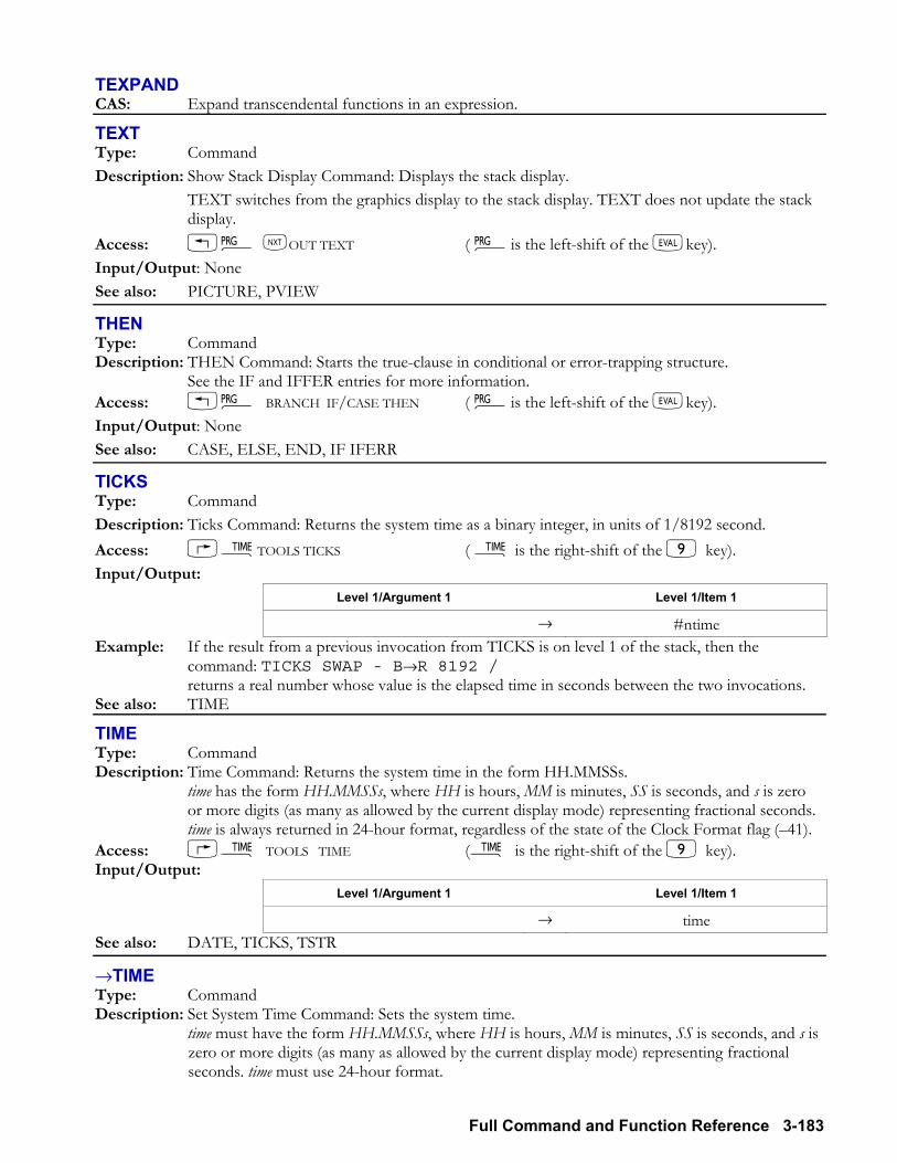
Full Command and Function Reference 3-183
TEXPAND CAS: Expand transcendental functions in an expression.
TEXT Type: Command Description: Show Stack Display Command: Displays the stack display. TEXT switches from the graphics display to the stack display. TEXT does not update the stack
display. Access: !° LOUT TEXT ( °is the left-shift of the Nkey). Input/Output: None See also: PICTURE, PVIEW
THEN Type: Command Description: THEN Command: Starts the true-clause in conditional or error-trapping structure. See the IF and IFFER entries for more information. Access: !° BRANCH IF/CASE THEN ( °is the left-shift of the Nkey). Input/Output: None See also: CASE, ELSE, END, IF IFERR
TICKS Type: Command Description: Ticks Command: Returns the system time as a binary integer, in units of 1/8192 second. Access: ÓTOOLS TICKS ( Ó is the right-shift of the 9 key). Input/Output:
Level 1/Argument 1 Level 1/Item 1
→ #ntime Example: If the result from a previous invocation from TICKS is on level 1 of the stack, then the
command: TICKS SWAP - B→R 8192 / returns a real number whose value is the elapsed time in seconds between the two invocations.
See also: TIME
TIME Type: Command Description: Time Command: Returns the system time in the form HH.MMSSs. time has the form HH.MMSSs, where HH is hours, MM is minutes, SS is seconds, and s is zero
or more digits (as many as allowed by the current display mode) representing fractional seconds. time is always returned in 24-hour format, regardless of the state of the Clock Format flag (41).
Access: Ó TOOLS TIME (Ó is the right-shift of the 9 key). Input/Output:
Level 1/Argument 1 Level 1/Item 1
→ time See also: DATE, TICKS, TSTR
→TIME Type: Command Description: Set System Time Command: Sets the system time. time must have the form HH.MMSSs, where HH is hours, MM is minutes, SS is seconds, and s is
zero or more digits (as many as allowed by the current display mode) representing fractional seconds. time must use 24-hour format.
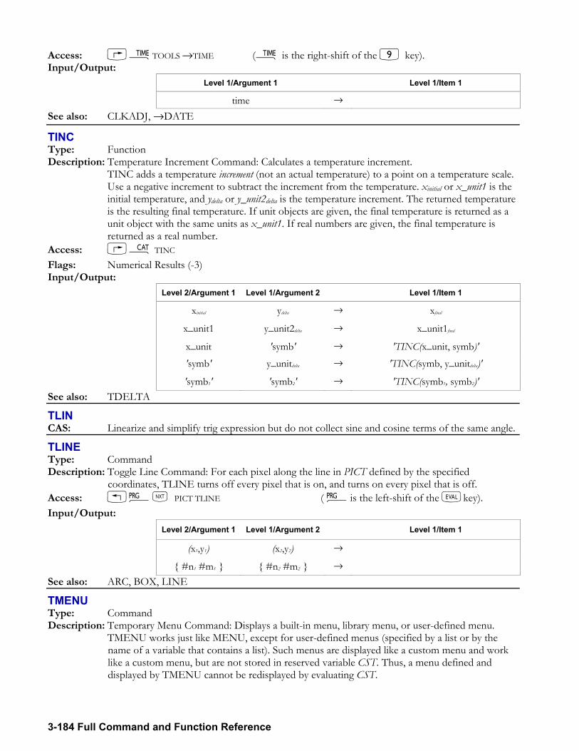
3-184 Full Command and Function Reference
Access: ÓTOOLS →TIME (Ó is the right-shift of the 9 key). Input/Output:
Level 1/Argument 1 Level 1/Item 1
time → See also: CLKADJ, →DATE
TINC Type: Function Description: Temperature Increment Command: Calculates a temperature increment. TINC adds a temperature increment (not an actual temperature) to a point on a temperature scale.
Use a negative increment to subtract the increment from the temperature. xinitial or x_unit1 is the initial temperature, and ydelta or y_unit2delta is the temperature increment. The returned temperature is the resulting final temperature. If unit objects are given, the final temperature is returned as a unit object with the same units as x_unit1. If real numbers are given, the final temperature is returned as a real number.
Access: µ TINC Flags: Numerical Results (-3) Input/Output:
Level 2/Argument 1 Level 1/Argument 2 Level 1/Item 1
xinitial ydelta → xfinal
x_unit1 y_unit2delta → x_unit1final
x_unit 'symb' → 'TINC(x_unit, symb)' 'symb' y_unitdelta → 'TINC(symb, y_unitdelta)'
'symb1' 'symb2' → 'TINC(symb1, symb2)' See also: TDELTA
TLIN CAS: Linearize and simplify trig expression but do not collect sine and cosine terms of the same angle.
TLINE Type: Command Description: Toggle Line Command: For each pixel along the line in PICT defined by the specified
coordinates, TLINE turns off every pixel that is on, and turns on every pixel that is off. Access: !°L PICT TLINE ( °is the left-shift of the Nkey). Input/Output:
Level 2/Argument 1 Level 1/Argument 2 Level 1/Item 1
(x1,y1) (x2,y2) →
#n1 #m1 #n2 #m2 →
See also: ARC, BOX, LINE
TMENU Type: Command Description: Temporary Menu Command: Displays a built-in menu, library menu, or user-defined menu. TMENU works just like MENU, except for user-defined menus (specified by a list or by the
name of a variable that contains a list). Such menus are displayed like a custom menu and work like a custom menu, but are not stored in reserved variable CST. Thus, a menu defined and displayed by TMENU cannot be redisplayed by evaluating CST.
Full Command and Function Reference 3-185
See Appendix H for a list of the hp49g+/hp48gII built-in menus and the corresponding menu numbers (xmenu).
Access: &H MENU TMENU Input/Output:
Level 1/Argument 1 Level 1/Item 1
xmenu →
listdefinition →
'namedefinition' → See also: MENU, RCLMENU
TOT Type: Command Description: Total Command: Computes the sum of each of the m columns of coordinate values in the
current statistics matrix (reserved variable ΣDAT). The sums are returned as a vector of m real numbers, or as a single real number if m = 1. Access: µ TOT Input/Output:
Level 1/Argument 1 Level 1/Item 1
→ xsum
→ [ xsum 1, xsum 2, ... ,xsum m ] See also: MAXΣ, MINΣ, MEAN, PSDEV, PVAR, SDEV, VAR
TRACE Type: Command Description: Matrix Trace Command: Returns the trace of a square matrix. The trace of a square matrix is the sum of its diagonal elements. Access: !Ø OPERATIONS LL TRACE ( Ø is the left-shift of the 5key). !´MATRIX NORMALIZE L TRACE ( ´ is the left-shift of the Pkey). Input/Output:
Level 1/Argument 1 Level 1/Item 1
[[ matrix ]]n×n → xtrace See also: CONJ, DET, IDN
TRAN Type: Command Description: Transpose Matrix Command: Returns the transpose of a matrix. Same as TRN, but without conjugation of complex numbers. Access: !Ø OPERATIONS LLTRAN ( Ø is the left-shift of the 5key). Input/Output:
Level 1/Argument 1 Level 1/Item 1
[[ matrix ]] → [[ matrix ]]transpose
'name' → See also: CONJ, TRN
TRANSIO Type: Command
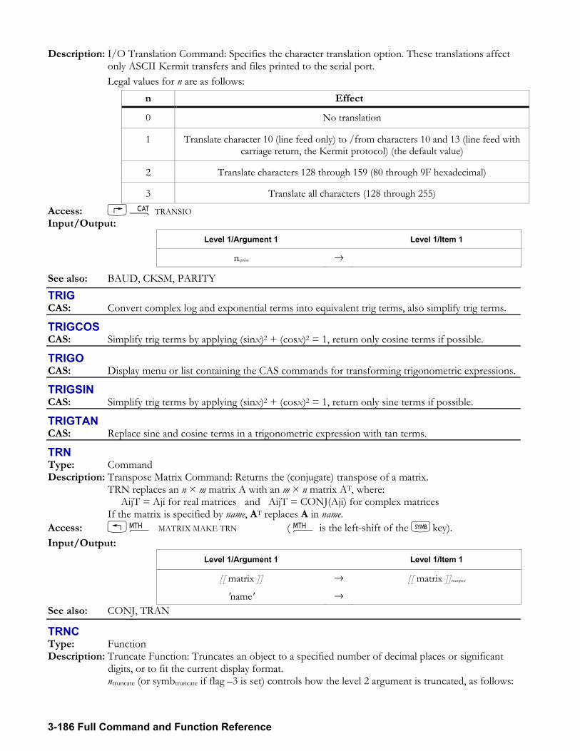
3-186 Full Command and Function Reference
Description: I/O Translation Command: Specifies the character translation option. These translations affect only ASCII Kermit transfers and files printed to the serial port.
Legal values for n are as follows: n Effect
0 No translation
1 Translate character 10 (line feed only) to /from characters 10 and 13 (line feed with carriage return, the Kermit protocol) (the default value)
2 Translate characters 128 through 159 (80 through 9F hexadecimal)
3 Translate all characters (128 through 255)
Access: µ TRANSIO Input/Output:
Level 1/Argument 1 Level 1/Item 1
noption →
See also: BAUD, CKSM, PARITY
TRIG CAS: Convert complex log and exponential terms into equivalent trig terms, also simplify trig terms.
TRIGCOS CAS: Simplify trig terms by applying (sinx)2 + (cosx)2 = 1, return only cosine terms if possible.
TRIGO CAS: Display menu or list containing the CAS commands for transforming trigonometric expressions.
TRIGSIN CAS: Simplify trig terms by applying (sinx)2 + (cosx)2 = 1, return only sine terms if possible.
TRIGTAN CAS: Replace sine and cosine terms in a trigonometric expression with tan terms.
TRN Type: Command Description: Transpose Matrix Command: Returns the (conjugate) transpose of a matrix. TRN replaces an n × m matrix A with an m × n matrix AT, where:
AijT = Aji for real matrices and AijT = CONJ(Aji) for complex matrices If the matrix is specified by name, AT replaces A in name. Access: !´ MATRIX MAKE TRN ( ´ is the left-shift of the Pkey). Input/Output:
Level 1/Argument 1 Level 1/Item 1
[[ matrix ]] → [[ matrix ]]transpose
'name' → See also: CONJ, TRAN
TRNC Type: Function Description: Truncate Function: Truncates an object to a specified number of decimal places or significant
digits, or to fit the current display format. ntruncate (or symbtruncate if flag 3 is set) controls how the level 2 argument is truncated, as follows:
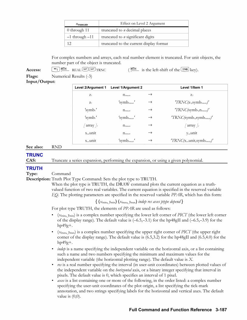
Full Command and Function Reference 3-187
ntruncate Effect on Level 2 Argument
0 through 11 truncated to n decimal places 1 through 11 truncated to n significant digits 12 truncated to the current display format
For complex numbers and arrays, each real number element is truncated. For unit objects, the
number part of the object is truncated. Access: !´ REAL LLTRNC ( ´ is the left-shift of the Pkey). Flags: Numerical Results (-3) Input/Output:
Level 2/Argument 1 Level 1/Argument 2 Level 1/Item 1
z1 ntruncate → z2
z1 'symbtruncate' → 'TRNC(z1,symbtruncate)'
'symb1' ntruncate → 'TRNC(symb1,ntruncate)'
'symb1' 'symbtruncate' → 'TRNC(symb1,symbtruncate)'
[ array ]1 ntruncate → [ array ]2
x_unit ntruncate → y_unit
x_unit 'symbtruncate' → 'TRNC(x_unit,symbtruncate)' See also: RND
TRUNC CAS: Truncate a series expansion, performing the expansion, or using a given polynomial.
TRUTH Type: Command Description: Truth Plot Type Command: Sets the plot type to TRUTH. When the plot type is TRUTH, the DRAW command plots the current equation as a truth-
valued function of two real variables. The current equation is specified in the reserved variable EQ. The plotting parameters are specified in the reserved variable PPAR, which has this form:
(xmin, ymin) (xmax, ymax) indep res axes ptype depend For plot type TRUTH, the elements of PPAR are used as follows:
(xmin, ymin) is a complex number specifying the lower left corner of PICT (the lower left corner of the display range). The default value is (6.5,3.1) for the hp48gII and (6.5,3.9) for the hp49g+.
(xmax, ymax) is a complex number specifying the upper right corner of PICT (the upper right corner of the display range). The default value is (6.5,3.2) for the hp48gII and (6.5,4.0) for the hp49g+.
indep is a name specifying the independent variable on the horizontal axis, or a list containing such a name and two numbers specifying the minimum and maximum values for the independent variable (the horizontal plotting range). The default value is X.
res is a real number specifying the interval (in user-unit coordinates) between plotted values of the independent variable on the horizontal axis, or a binary integer specifying that interval in pixels. The default value is 0, which specifies an interval of 1 pixel.
axes is a list containing one or more of the following, in the order listed: a complex number specifying the user-unit coordinates of the plot origin, a list specifying the tick-mark annotation, and two strings specifying labels for the horizontal and vertical axes. The default value is (0,0).
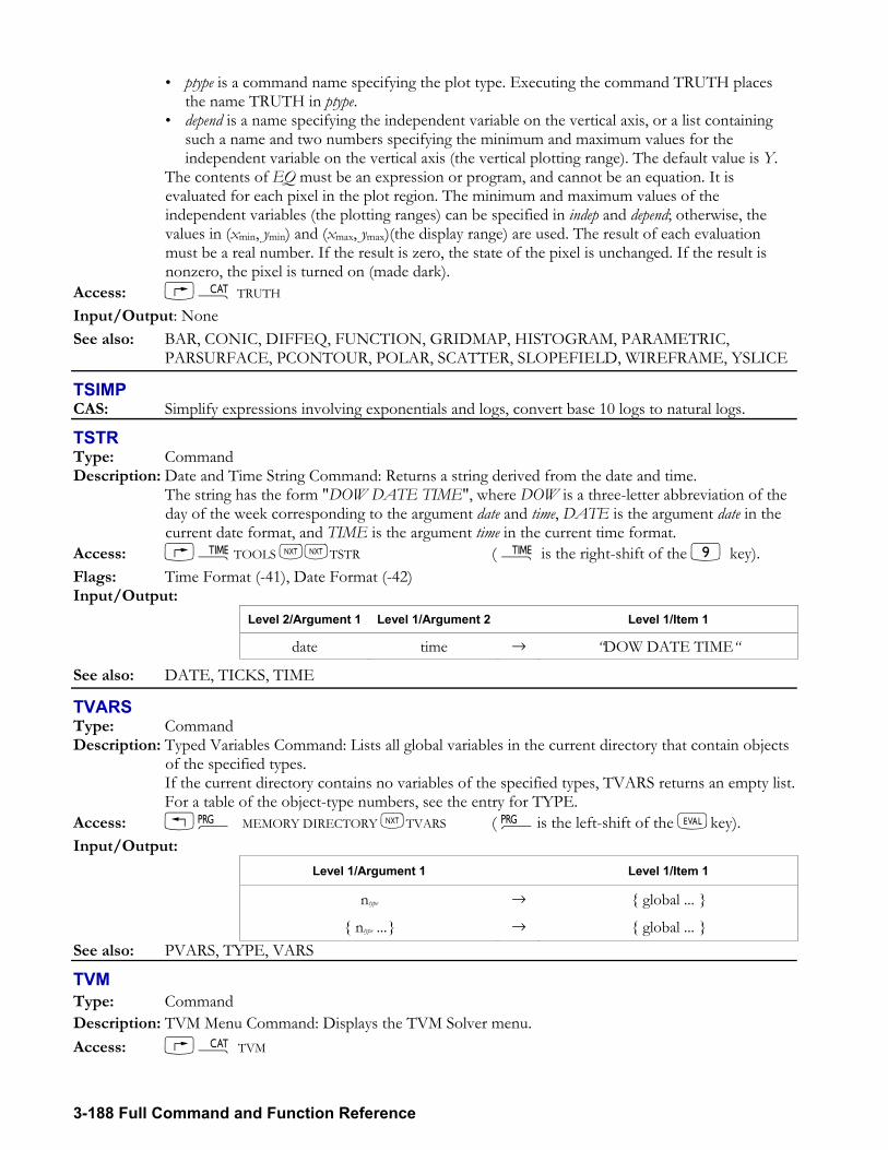
3-188 Full Command and Function Reference
ptype is a command name specifying the plot type. Executing the command TRUTH places the name TRUTH in ptype.
depend is a name specifying the independent variable on the vertical axis, or a list containing such a name and two numbers specifying the minimum and maximum values for the independent variable on the vertical axis (the vertical plotting range). The default value is Y.
The contents of EQ must be an expression or program, and cannot be an equation. It is evaluated for each pixel in the plot region. The minimum and maximum values of the independent variables (the plotting ranges) can be specified in indep and depend; otherwise, the values in (xmin, ymin) and (xmax, ymax)(the display range) are used. The result of each evaluation must be a real number. If the result is zero, the state of the pixel is unchanged. If the result is nonzero, the pixel is turned on (made dark).
Access: µ TRUTH Input/Output: None See also: BAR, CONIC, DIFFEQ, FUNCTION, GRIDMAP, HISTOGRAM, PARAMETRIC,
PARSURFACE, PCONTOUR, POLAR, SCATTER, SLOPEFIELD, WIREFRAME, YSLICE
TSIMP CAS: Simplify expressions involving exponentials and logs, convert base 10 logs to natural logs.
TSTR Type: Command Description: Date and Time String Command: Returns a string derived from the date and time. The string has the form "DOW DATE TIME", where DOW is a three-letter abbreviation of the
day of the week corresponding to the argument date and time, DATE is the argument date in the current date format, and TIME is the argument time in the current time format.
Access: ÓTOOLS LLTSTR ( Ó is the right-shift of the 9 key). Flags: Time Format (-41), Date Format (-42) Input/Output:
Level 2/Argument 1 Level 1/Argument 2 Level 1/Item 1
date time → DOW DATE TIME
See also: DATE, TICKS, TIME
TVARS Type: Command Description: Typed Variables Command: Lists all global variables in the current directory that contain objects
of the specified types. If the current directory contains no variables of the specified types, TVARS returns an empty list. For a table of the object-type numbers, see the entry for TYPE. Access: !° MEMORY DIRECTORY LTVARS ( °is the left-shift of the Nkey). Input/Output:
Level 1/Argument 1 Level 1/Item 1
ntype → global ...
ntype ... → global ... See also: PVARS, TYPE, VARS
TVM Type: Command Description: TVM Menu Command: Displays the TVM Solver menu. Access: µ TVM
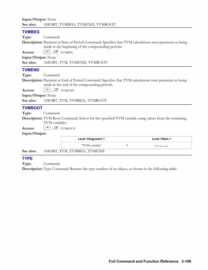
Full Command and Function Reference 3-189
Input/Output: None See also: AMORT, TVMBEG, TVMEND, TVMROOT
TVMBEG Type: Command Description: Payment at Start of Period Command: Specifies that TVM calculations treat payments as being
made at the beginning of the compounding periods. Access: µ TVMBEG Input/Output: None See also: AMORT, TVM, TVMEND, TVMROOT
TVMEND Type: Command Description: Payment at End of Period Command: Specifies that TVM calculations treat payments as being
made at the end of the compounding periods. Access: µ TVMEND Input/Output: None See also: AMORT, TVM, TVMBEG, TVMROOT
TVMROOT Type: Command Description: TVM Root Command: Solves for the specified TVM variable using values from the remaining
TVM variables. Access: µ TVMROOT Input/Output:
Level 1/Argument 1 Level 1/Item 1
'TVM variable' → xTVM variable
See also: AMORT, TVM, TVMBEG, TVMEND
TYPE Type: Command Description: Type Command: Returns the type number of an object, as shown in the following table:
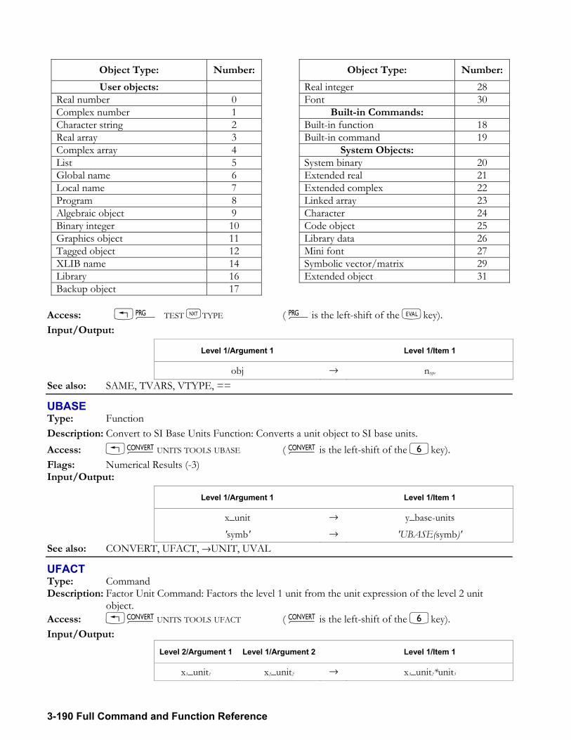
3-190 Full Command and Function Reference
Object Type: Number: Object Type: Number:User objects: Real integer 28
Real number 0 Font 30 Complex number 1 Built-in Commands: Character string 2 Built-in function 18 Real array 3 Built-in command 19 Complex array 4 System Objects: List 5 System binary 20 Global name 6 Extended real 21 Local name 7 Extended complex 22 Program 8 Linked array 23 Algebraic object 9 Character 24 Binary integer 10 Code object 25 Graphics object 11 Library data 26 Tagged object 12 Mini font 27 XLIB name 14 Symbolic vector/matrix 29 Library 16 Extended object 31 Backup object 17
Access: !° TEST LTYPE ( °is the left-shift of the Nkey). Input/Output:
Level 1/Argument 1 Level 1/Item 1
obj → ntype See also: SAME, TVARS, VTYPE, ==
UBASE Type: Function Description: Convert to SI Base Units Function: Converts a unit object to SI base units. Access: !Ú UNITS TOOLS UBASE ( Ú is the left-shift of the 6key). Flags: Numerical Results (-3) Input/Output:
Level 1/Argument 1 Level 1/Item 1
x_unit → y_base-units
'symb' → 'UBASE(symb)' See also: CONVERT, UFACT, →UNIT, UVAL
UFACT Type: Command Description: Factor Unit Command: Factors the level 1 unit from the unit expression of the level 2 unit
object. Access: !Ú UNITS TOOLS UFACT ( Ú is the left-shift of the 6key). Input/Output:
Level 2/Argument 1 Level 1/Argument 2 Level 1/Item 1
x1_unit1 x2_unit2 → x3_unit2*unit3
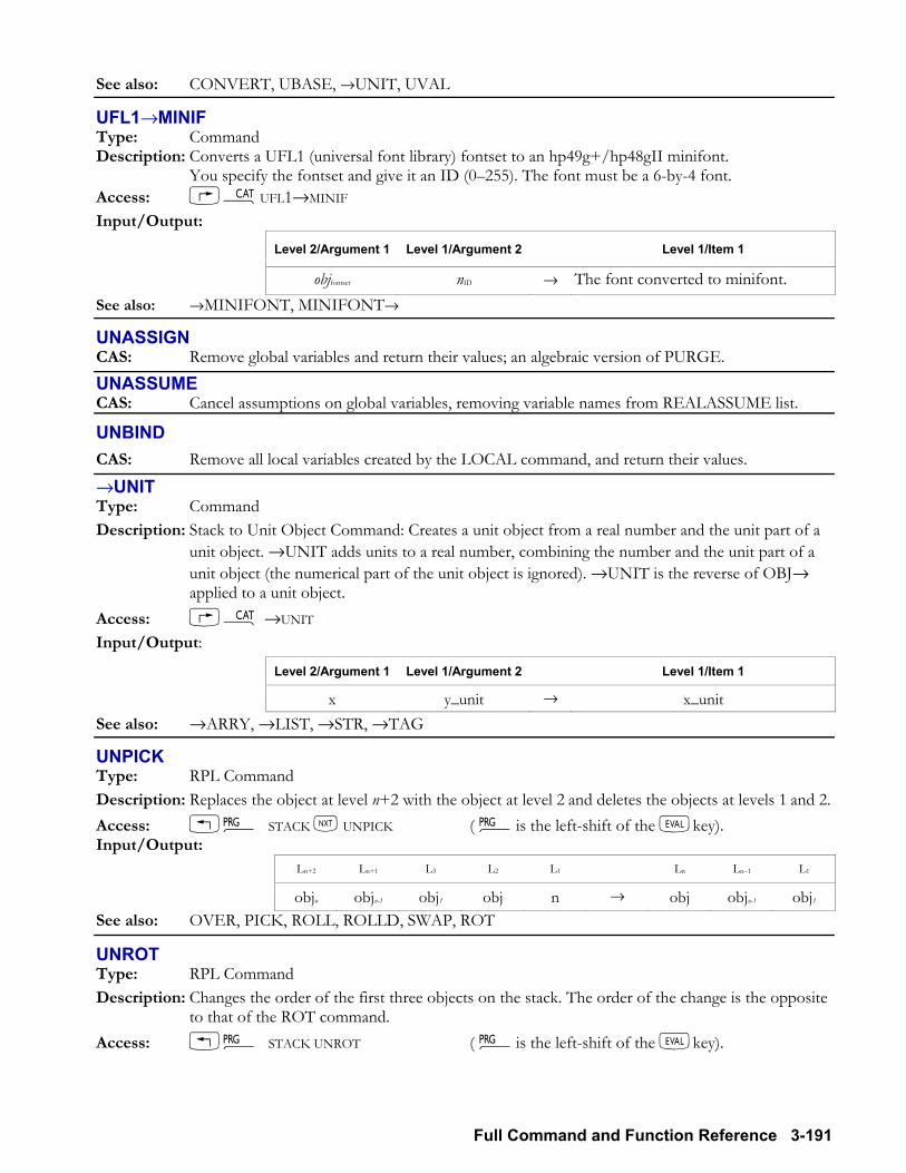
Full Command and Function Reference 3-191
See also: CONVERT, UBASE, →UNIT, UVAL
UFL1→MINIF Type: Command Description: Converts a UFL1 (universal font library) fontset to an hp49g+/hp48gII minifont. You specify the fontset and give it an ID (0255). The font must be a 6-by-4 font. Access: µUFL1→MINIF Input/Output:
Level 2/Argument 1 Level 1/Argument 2 Level 1/Item 1
objfontset nID → The font converted to minifont. See also: →MINIFONT, MINIFONT→
UNASSIGN CAS: Remove global variables and return their values; an algebraic version of PURGE.
UNASSUME CAS: Cancel assumptions on global variables, removing variable names from REALASSUME list.
UNBIND CAS: Remove all local variables created by the LOCAL command, and return their values.
→UNIT Type: Command Description: Stack to Unit Object Command: Creates a unit object from a real number and the unit part of a
unit object. →UNIT adds units to a real number, combining the number and the unit part of a unit object (the numerical part of the unit object is ignored). →UNIT is the reverse of OBJ→ applied to a unit object.
Access: µ →UNIT Input/Output:
Level 2/Argument 1 Level 1/Argument 2 Level 1/Item 1
x y_unit → x_unit See also: →ARRY, →LIST, →STR, →TAG
UNPICK Type: RPL Command Description: Replaces the object at level n+2 with the object at level 2 and deletes the objects at levels 1 and 2. Access: !° STACK L UNPICK ( °is the left-shift of the Nkey). Input/Output:
Ln+2 Ln+1 L3 L2 L1 Ln Ln1 L1
objn objn-1 obj1 obj n → obj objn-1 obj1 See also: OVER, PICK, ROLL, ROLLD, SWAP, ROT
UNROT Type: RPL Command Description: Changes the order of the first three objects on the stack. The order of the change is the opposite
to that of the ROT command. Access: !° STACK UNROT ( °is the left-shift of the Nkey).
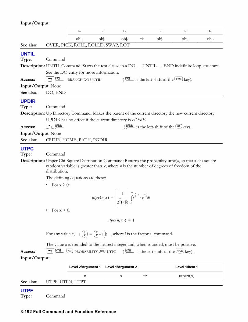
3-192 Full Command and Function Reference
Γ z2---⎝ ⎠⎛ ⎞ z
2--- 1⎝ ⎠⎛ ⎞ !=
Input/Output: L3 L2 L1 L3 L2 L1
obj3 obj2 obj1 → obj1 obj3 obj2 See also: OVER, PICK, ROLL, ROLLD, SWAP, ROT
UNTIL Type: Command Description: UNTIL Command: Starts the test clause in a DO UNTIL END indefinite loop structure. See the DO entry for more information. Access: !° BRANCH DO UNTIL ( °is the left-shift of the Nkey). Input/Output: None See also: DO, END
UPDIR Type: Command Description: Up Directory Command: Makes the parent of the current directory the new current directory. UPDIR has no effect if the current directory is HOME. Access: !§ ( §is the left-shift of the Jkey). Input/Output: None See also: CRDIR, HOME, PATH, PGDIR
UTPC Type: Command Description: Upper Chi-Square Distribution Command: Returns the probability utpc(n, x) that a chi-square
random variable is greater than x, where n is the number of degrees of freedom of the distribution.
The defining equations are these: For x ≥ 0:
utpc n x,( )1
2n2---Γ n
2---( )
---------------- tn2--- 1
et2---
⋅ tdx
∞
∫=
For x < 0:
utpc n x ),( ) 1=
For any value z, , where ! is the factorial command.
The value n is rounded to the nearest integer and, when rounded, must be positive. Access: !´ L PROBABILITY L UTPC ( ´ is the left-shift of the Pkey). Input/Output:
Level 2/Argument 1 Level 1/Argument 2 Level 1/Item 1
n x → utpc(n,x) See also: UTPF, UTPN, UTPT
UTPF Type: Command
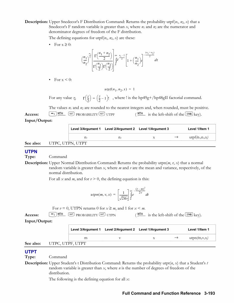
Full Command and Function Reference 3-193
Γ z2---⎝ ⎠⎛ ⎞ z
2--- 1⎝ ⎠⎛ ⎞ !=
Description: Upper Snedecor's F Distribution Command: Returns the probability utpf(n1, n2, x) that a Snedecor's F random variable is greater than x, where n1 and n2 are the numerator and denominator degrees of freedom of the F distribution.
The defining equations for utpf(n1, n2, x) are these: For x ≥ 0:
n1n2-----⎝ ⎠⎛ ⎞
n12----- Γ
n1 n2+2-----------------⎝ ⎠
⎛ ⎞
Γn12-----⎝ ⎠
⎛ ⎞Γn22-----⎝ ⎠
⎛ ⎞------------------------------ t
n1 22--------------
x
∞
∫ 1n1n2-----⎝ ⎠⎛ ⎞ t+
n1 n2+( )
2-----------------------
dt
For x < 0:
utpf n1 n2 x, ,( ) 1=
For any value z, , where ! is the hp49g+/hp48gII factorial command. The values n1 and n2 are rounded to the nearest integers and, when rounded, must be positive. Access: !´ L PROBABILITY L UTPF ( ´ is the left-shift of the Pkey). Input/Output:
Level 3/Argument 1 Level 2/Argument 2 Level 1/Argument 3 Level 1/Item 1
n1 n2 x → utpf(n1,n2,x) See also: UTPC, UTPN, UTPT
UTPN Type: Command Description: Upper Normal Distribution Command: Returns the probability utpn(m, v, x) that a normal
random variable is greater than x, where m and v are the mean and variance, respectively, of the normal distribution.
For all x and m, and for v > 0, the defining equation is this:
utpn m v x, ,( ) 12πv
------------- et m( )2
2v------------------td
x
∞
∫=
For v = 0, UTPN returns 0 for x ≥ m, and 1 for x < m. Access: !´ L PROBABILITY L UTPN ( ´ is the left-shift of the Pkey). Input/Output:
Level 3/Argument 1 Level 2/Argument 2 Level 1/Argument 3 Level 1/Item 1
m v x → utpn(m,v,x) See also: UTPC, UTPF, UTPT
UTPT Type: Command Description: Upper Student's t Distribution Command: Returns the probability utpt(n, x) that a Student's t
random variable is greater than x, where n is the number of degrees of freedom of the distribution.
The following is the defining equation for all x:
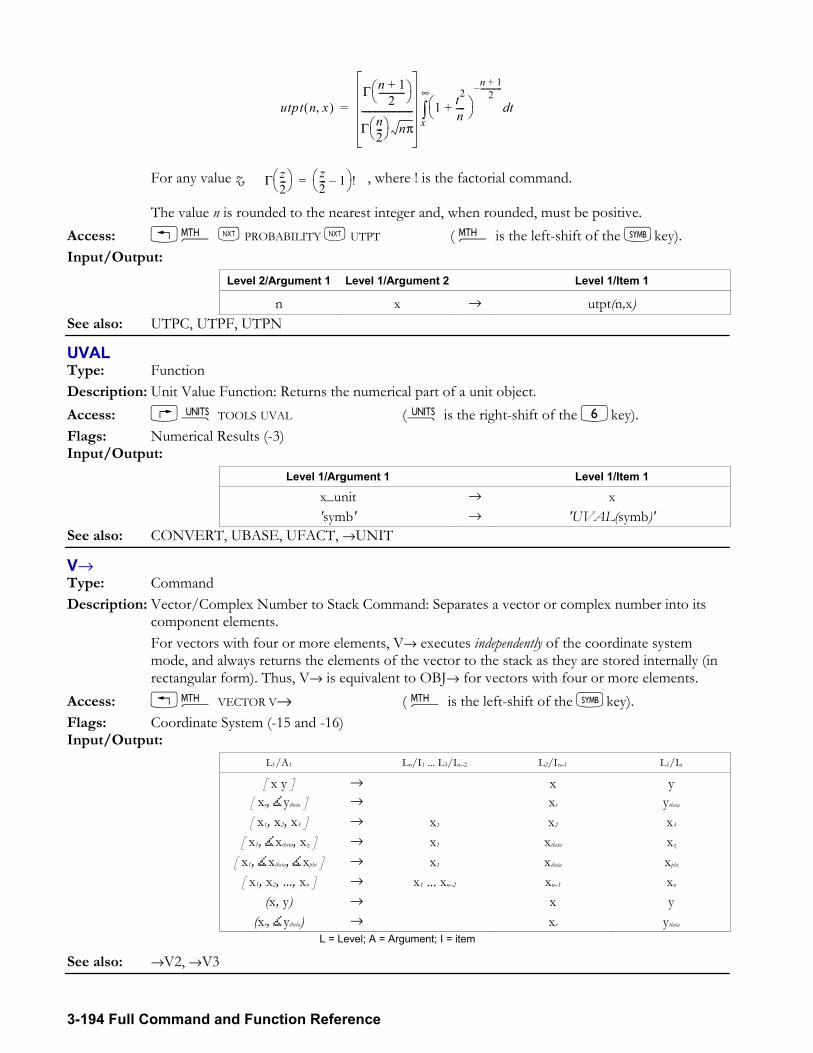
3-194 Full Command and Function Reference
Γ z2---⎝ ⎠⎛ ⎞ z
2--- 1⎝ ⎠⎛ ⎞ !=
utpt n x,( )Γ n 1+
2------------⎝ ⎠⎛ ⎞
Γ n2---⎝ ⎠⎛ ⎞ nπ
----------------------- 1 t2
n----+⎝ ⎠⎛ ⎞
n 1+2
------------
tdx
∞
∫=
For any value z, , where ! is the factorial command. The value n is rounded to the nearest integer and, when rounded, must be positive. Access: !´ L PROBABILITY L UTPT ( ´ is the left-shift of the Pkey). Input/Output:
Level 2/Argument 1 Level 1/Argument 2 Level 1/Item 1
n x → utpt(n,x) See also: UTPC, UTPF, UTPN
UVAL Type: Function Description: Unit Value Function: Returns the numerical part of a unit object. Access: Û TOOLS UVAL (Û is the right-shift of the 6key). Flags: Numerical Results (-3) Input/Output:
Level 1/Argument 1 Level 1/Item 1
x_unit → x 'symb' → 'UVAL(symb)'
See also: CONVERT, UBASE, UFACT, →UNIT
V→ Type: Command Description: Vector/Complex Number to Stack Command: Separates a vector or complex number into its
component elements. For vectors with four or more elements, V→ executes independently of the coordinate system
mode, and always returns the elements of the vector to the stack as they are stored internally (in rectangular form). Thus, V→ is equivalent to OBJ→ for vectors with four or more elements.
Access: !´ VECTOR V→ ( ´ is the left-shift of the Pkey). Flags: Coordinate System (-15 and -16) Input/Output:
L1/A1 Ln/I1 ... L3/In2 L2/In1 L1/In [ x y ] → x y
[ xr, ytheta ] → xr ytheta [ x1, x2, x3 ] → x1 x2 x3
[ x1, xtheta, xz ] → x1 xtheta xz [ x1, xtheta, xphi ] → x1 xtheta xphi
[ x1, x2, ..., xn ] → x1 ... xn2 xn1 xn (x, y) → x y
(xr, ytheta) → xr ytheta L = Level; A = Argument; I = item
See also: →V2, →V3
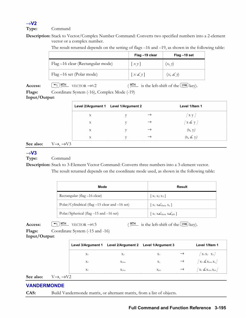
Full Command and Function Reference 3-195
→V2 Type: Command Description: Stack to Vector/Complex Number Command: Converts two specified numbers into a 2-element
vector or a complex number. The result returned depends on the setting of flags 16 and 19, as shown in the following table:
Flag 19 clear Flag 19 set
Flag 16 clear (Rectangular mode) [ x y ] (x, y)
Flag 16 set (Polar mode) [ x y ] (x, y)
Access: !´ VECTOR →V2 ( ´ is the left-shift of the Pkey). Flags: Coordinate System (-16), Complex Mode (-19) Input/Output:
Level 2/Argument 1 Level 1/Argument 2 Level 1/Item 1
x y → [ x y ] x y → [ x y ]
x y → (x, y) x y → (x, y)
See also: V→, →V3
→V3 Type: Command Description: Stack to 3-Element Vector Command: Converts three numbers into a 3-element vector. The result returned depends on the coordinate mode used, as shown in the following table:
Mode Result
Rectangular (flag 16 clear) [ x1 x2 x3 ]
Polar/Cylindrical (flag 15 clear and 16 set) [ x1 xtheta xz ]
Polar/Spherical (flag 15 and 16 set) [ x1 xtheta xphi ]
Access: !´ VECTOR →V3 ( ´ is the left-shift of the Pkey). Flags: Coordinate System (-15 and -16) Input/Output:
Level 3/Argument 1 Level 2/Argument 2 Level 1/Argument 3 Level 1/Item 1
x1 x2 x3 → [ x1 x2 x3 ]
x1 xtheta xz → [ x1 xtheta xz ]
x1 xtheta xphi → [ x1 xtheta xphi ]
See also: V→, →V2
VANDERMONDE CAS: Build Vandermonde matrix, or alternant matrix, from a list of objects.
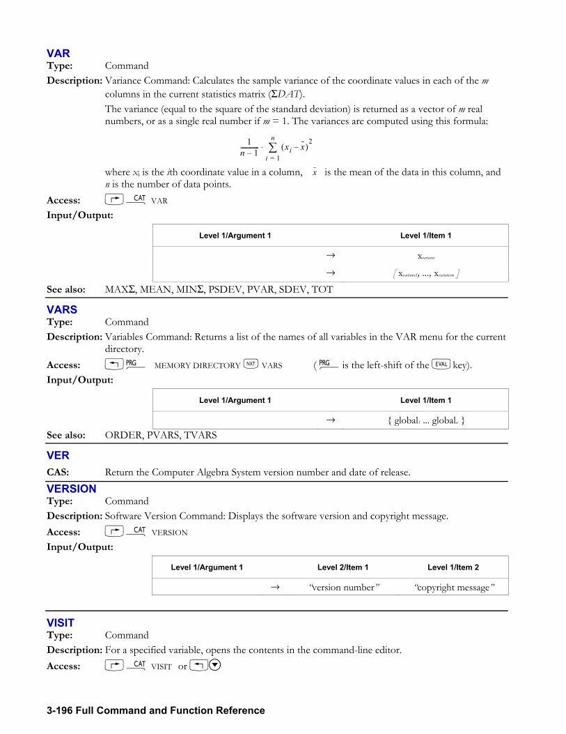
3-196 Full Command and Function Reference
x
VAR Type: Command Description: Variance Command: Calculates the sample variance of the coordinate values in each of the m
columns in the current statistics matrix (ΣDAT). The variance (equal to the square of the standard deviation) is returned as a vector of m real
numbers, or as a single real number if m = 1. The variances are computed using this formula:
1n 1------------ xi x( )
2
i 1=
n∑⋅
where xi is the ith coordinate value in a column, is the mean of the data in this column, and
n is the number of data points. Access: µ VAR Input/Output:
Level 1/Argument 1 Level 1/Item 1
→ xvariance
→ [ xvariance1, ..., xvariancem ] See also: MAXΣ, MEAN, MINΣ, PSDEV, PVAR, SDEV, TOT
VARS Type: Command Description: Variables Command: Returns a list of the names of all variables in the VAR menu for the current
directory. Access: !° MEMORY DIRECTORY L VARS ( °is the left-shift of the Nkey). Input/Output:
Level 1/Argument 1 Level 1/Item 1
→ global1 ... globaln See also: ORDER, PVARS, TVARS
VER CAS: Return the Computer Algebra System version number and date of release.
VERSION Type: Command Description: Software Version Command: Displays the software version and copyright message. Access: µ VERSION Input/Output:
Level 1/Argument 1 Level 2/Item 1 Level 1/Item 2
→ version number copyright message
VISIT Type: Command Description: For a specified variable, opens the contents in the command-line editor. Access: µ VISIT or
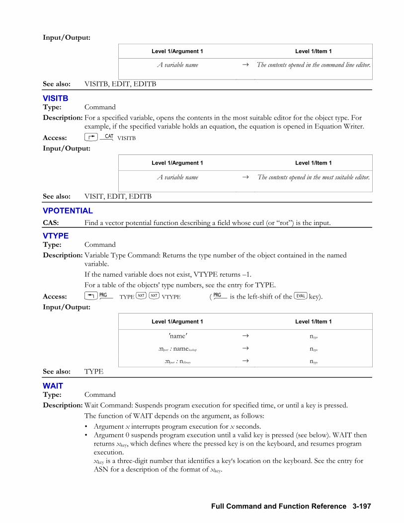
Full Command and Function Reference 3-197
Input/Output:
Level 1/Argument 1 Level 1/Item 1
A variable name → The contents opened in the command line editor.
See also: VISITB, EDIT, EDITB
VISITB Type: Command Description: For a specified variable, opens the contents in the most suitable editor for the object type. For
example, if the specified variable holds an equation, the equation is opened in Equation Writer. Access: µ VISITB Input/Output:
Level 1/Argument 1 Level 1/Item 1
A variable name → The contents opened in the most suitable editor.
See also: VISIT, EDIT, EDITB
VPOTENTIAL CAS: Find a vector potential function describing a field whose curl (or rot) is the input.
VTYPE Type: Command Description: Variable Type Command: Returns the type number of the object contained in the named
variable. If the named variable does not exist, VTYPE returns 1. For a table of the objects' type numbers, see the entry for TYPE. Access: !° TYPE L L VTYPE ( °is the left-shift of the Nkey). Input/Output:
Level 1/Argument 1 Level 1/Item 1
'name' → ntype
:nport : namebackup → ntype
:nport : nlibrary → ntype See also: TYPE
WAIT Type: Command Description: Wait Command: Suspends program execution for specified time, or until a key is pressed. The function of WAIT depends on the argument, as follows:
Argument x interrupts program execution for x seconds. Argument 0 suspends program execution until a valid key is pressed (see below). WAIT then
returns xkey, which defines where the pressed key is on the keyboard, and resumes program execution. xkey is a three-digit number that identifies a key's location on the keyboard. See the entry for ASN for a description of the format of xkey.
3-198 Full Command and Function Reference
Argument 1 works as with argument 0, except that the currently specified menu is also displayed.
!, , ~, ~!, and ~ are not by themselves valid keys. Arguments 0 and 1 do not affect the display, so that messages persist even though the keyboard
is ready for input (FREEZE is not required). Normally, the MENU command does not update the menu keys until a program halts or ends.
WAIT with argument 1 enables a previous execution of MENU to display that menu while the program is suspended for a key press.
Access: !° L IN WAIT ( °is the left-shift of the Nkey). Input/Output:
Level 1/Argument 1 Level 1/Item 1
x →
0 → xkey
1 → xkey See also: KEY
WHILE Type: Command Operation Description: WHILE Indefinite Loop Structure Command: Starts the WHILE REPEAT END
indefinite loop structure. WHILE REPEAT END repeatedly evaluates a test and executes a loop clause if the test is
true. Since the test clause occurs before the loop-clause, the loop clause is never executed if the test is initially false. The syntax is this:
WHILE test-clause REPEAT loop-clause END The test clause is executed and must return a test result to the stack. REPEAT takes the value
from the stack. If the value is not zero, execution continues with the loop clause; otherwise, execution resumes following END.
Access: !° BRANCH WHILE ( °is the left-shift of the Nkey). Input/Output:
Level 1/Argument 1 Level 1/Item 1
WHILE →
REPEAT T/F →
END →
See also: DO, END, REPEAT
WIREFRAME Type: Command Description: WIREFRAME Plot Type Command: Sets the plot type to WIREFRAME. When the plot type is set to WIREFRAME, the DRAW command plots a perspective view of
the graph of a scalar function of two variables. WIREFRAME requires values in the reserved variables EQ, VPAR, and PPAR.
VPAR has the following form: xleft, xright, ynear, yfar, zlow, zhigh, xmin, xmax, ymin, ymax, xeye, yeye, zeye, xstep, ystep For plot type WIREFRAME, the elements of VPAR are used as follows:
Full Command and Function Reference 3-199
xleft and xright are real numbers that specify the width of the view space. ynear and yfar are real numbers that specify the depth of the view space. zlow and zhigh are real numbers that specify the height of the view space. xmin and xmax are not used. ymin and ymax are not used. xeye, yeye, and zeye are real numbers that specify the point in space from which the graph is
viewed. xstep and ystep are real numbers that set the number of x-coordinates versus the number of y-
coordinates plotted. The plotting parameters are specified in the reserved variable PPAR, which has this form:
(xmin, ymin) (xmax, ymax) indep res axes ptype depend For plot type WIREFRAME, the elements of PPAR are used as follows:
(xmin, ymin) is not used. (xmax, ymax) is not used. indep is a name specifying the independent variable. The default value of indep is X. res is not used. axes is not used. ptype is a name specifying the plot type. Executing the command WIREFRAME places the
command name WIREFRAME in ptype. depend is a name specifying the dependent variable. The default value is Y.
Access: µ WIREFRAME Input/Output: None See also: BAR, CONIC DIFFEQ, FUNCTION, GRIDMAP, HISTOGRAM, PARAMETRIC,
PARSURFACE, PCONTOUR, POLAR, SCATTER, SLOPEFIELD, TRUTH, YSLICE
WSLOG Type: Command Description: Warmstart Log Command: Returns four strings recording the date, time, and cause of the four
most recent warmstart events. Each string "logn" has the form "codedate time". The following table summarizes the legal values
of code and their meanings. Code Description
0 The warmstart log was cleared by pressing $.
1 The interrupt system detected a very low battery condition at the battery contacts (not the same as a low system voltage), and put the calculator in Deep Sleep mode (with the system clock running). When $ is pressed after the battery voltage is restored, the system warmstarts and puts a 1 in the log.
2 Hardware failed during transmission (timeout).
3 Run through address 0.
4 System time is corrupt
5 A Deep Sleep wakeup (for example, $, Alarm).
6 Not used
3-200 Full Command and Function Reference
Code Description
7 A 5-nibble word (CMOS test word) in RAM was corrupt. (This word is checked on every interrupt, but it is used only as an indicator of potentially corrupt RAM.)
8 Not used
9 The alarm list is corrupt.
A System RPL jump to #0.
B The card module was removed (or card bounce).
C Hardware reset occurred (for example, an electrostatic discharge or user reset)
D An expected System (RPL) error handler was not found in runstream The date and time stamp (date time) part of the log may be displayed as 000000 for one of three
reasons: The system time was corrupt when the stamp was recorded. The date and time stamp itself is corrupt (bad checksum). Fewer than four warmstarts have occurred since the log was last cleared.
Access: µ WSLOG Flags: Date Format (-42) Input/Output:
Level 1/Argument 1 Level 4/Item 1 ... Level 1/Item 4
→ log4 ... log1
ΣX Type: Command Description: Sum of x-Values Command: Sums the values in the independent-variable column of the current
statistical matrix (reserved variable ΣDAT). The independent-variable column is specified by XCOL and is stored as the first parameter in
the reserved variable ΣPAR. The default independent-variable column number is 1. Access: µΣX Input/Output:
Level 1/Argument 1 Level 1/Item 1
→ xsum See also: NΣ, XCOL, ΣXY, ΣX2, ΣY, ΣY2
ΣX2 Type: Command Description: Sum of Squares of x-Values Command: Sums the squares of the values in the independent-
variable column of the current statistical matrix (reserved variable ΣDAT). The independent-variable column is specified by XCOL and is stored as the first parameter in
the reserved variable ΣPAR. The default independent-variable column number is 1. Access: µΣX2
Full Command and Function Reference 3-201
Input/Output: Level 1/Argument 1 Level 1/Item 1
→ Sum of X2 See also: NΣ, ΣX, XCOL, ΣXY, ΣY, ΣY2
XCOL Type: Command Description: Independent Column Command: Specifies the independent-variable column of the current
statistics matrix (reserved variable ΣDAT). The independent-variable column number is stored as the first parameter in the reserved variable
ΣPAR. The default independent-variable column number is 1. XCOL will accept a noninteger real number and store it in ΣPAR, but subsequent commands
that utilize the XCOL specification in ΣPAR will cause an error. Access: µXCOL Input/Output:
Level 1/Argument 1 Level 1/Item 1
ncol → See also: BARPLOT, BESTFIT, COLΣ, CORR, COV, EXPFIT, HISTPLOT, LINFIT, LOGFIT, LR,
PREDX, PREDY, PWRFIT, SCATRPLOT, YCOL
XGET Type: Command Description: XModem Get Command: Retrieves a specified filename via XMODEM from another calculator.
The other calculator needs to be in server mode for the operation to work (G I/O FUNCTIONS START SERVER).
Access: µ XGET Input/Output:
Level 1/Argument 1 Level 1/Item 1
'name' → See also: BAUD, RECN, RECV, SEND XRECV, XSERV, XPUT
XMIT Type: Command Description: Serial Transmit Command: Sends a string serially without using Kermit protocol, and returns a
single digit that indicates whether the transmission was successful. XMIT is useful for communicating with non-Kermit devices such as RS-232 printers. If the transmission is successful, XMIT returns a 1. If the transmission is not successful, XMIT
returns the unsent portion of the string and a 0. Use ERRM to get the error message. After receiving an XOFF command (with transmit pacing in the reserved variable IOPAR set),
XMIT stops transmitting and waits for an XON command. XMIT resumes transmitting if an XON is received before the time-out set by STIME elapses; otherwise, XMIT terminates, returns a 0, and stores "Timeout" in ERRM.
Access: µ XMIT Flags: I/O Device (-33)
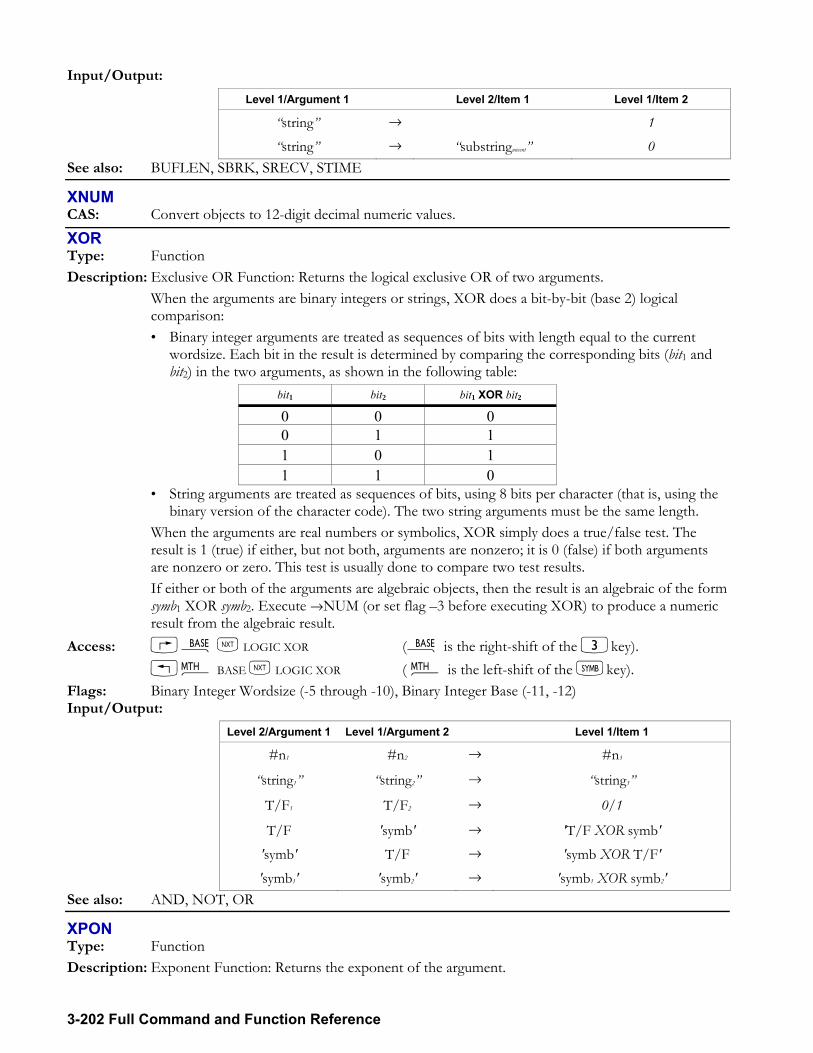
3-202 Full Command and Function Reference
Input/Output: Level 1/Argument 1 Level 2/Item 1 Level 1/Item 2
string → 1 string → substringunsent 0
See also: BUFLEN, SBRK, SRECV, STIME
XNUM CAS: Convert objects to 12-digit decimal numeric values.
XOR Type: Function Description: Exclusive OR Function: Returns the logical exclusive OR of two arguments. When the arguments are binary integers or strings, XOR does a bit-by-bit (base 2) logical
comparison: Binary integer arguments are treated as sequences of bits with length equal to the current
wordsize. Each bit in the result is determined by comparing the corresponding bits (bit1 and bit2) in the two arguments, as shown in the following table:
bit1 bit2 bit1 XOR bit2 0 0 00 1 1 1 0 1 1 1 0
String arguments are treated as sequences of bits, using 8 bits per character (that is, using the binary version of the character code). The two string arguments must be the same length.
When the arguments are real numbers or symbolics, XOR simply does a true/false test. The result is 1 (true) if either, but not both, arguments are nonzero; it is 0 (false) if both arguments are nonzero or zero. This test is usually done to compare two test results.
If either or both of the arguments are algebraic objects, then the result is an algebraic of the form symb1 XOR symb2. Execute →NUM (or set flag 3 before executing XOR) to produce a numeric result from the algebraic result.
Access: ã L LOGIC XOR (ã is the right-shift of the 3key). !´ BASE L LOGIC XOR ( ´ is the left-shift of the Pkey). Flags: Binary Integer Wordsize (-5 through -10), Binary Integer Base (-11, -12) Input/Output:
Level 2/Argument 1 Level 1/Argument 2 Level 1/Item 1
#n1 #n2 → #n3
string1 string2 → string3
T/F1 T/F2 → 0/1
T/F 'symb' → 'T/F XOR symb' 'symb' T/F → 'symb XOR T/F' 'symb1' 'symb2' → 'symb1 XOR symb2'
See also: AND, NOT, OR
XPON Type: Function Description: Exponent Function: Returns the exponent of the argument.
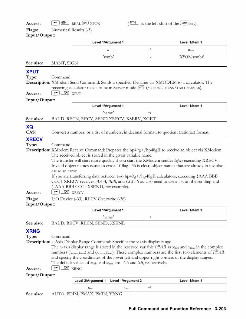
Full Command and Function Reference 3-203
Access: !´ REAL L XPON ( ´ is the left-shift of the Pkey). Flags: Numerical Results (-3) Input/Output:
Level 1/Argument 1 Level 1/Item 1
x → nexpon
'symb' → 'XPON(symb)' See also: MANT, SIGN
XPUT Type: Command Description: XModem Send Command: Sends a specified filename via XMODEM to a calculator. The
receiving calculator needs to be in Server mode (G I/O FUNCTIONS START SERVER). Access: µ XPUT Input/Output:
Level 1/Argument 1 Level 1/Item 1
'name' → See also: BAUD, RECN, RECV, SEND XRECV, XSERV, XGET
XQ CAS: Convert a number, or a list of numbers, in decimal format, to quotient (rational) format.
XRECV Type: Command Description: XModem Receive Command: Prepares the hp49g+/hp48gII to receive an object via XModem.
The received object is stored in the given variable name. The transfer will start more quickly if you start the XModem sender before executing XRECV. Invalid object names cause an error. If flag 36 is clear, object names that are already in use also
cause an error. If you are transferring data between two hp49g+/hp48gII calculators, executing AAA BBB
CCC XRECV receives AAA, BBB, and CCC. You also need to use a list on the sending end (AAA BBB CCC XSEND, for example).
Access: µ XRECV Flags: I/O Device (-33), RECV Overwrite (-36) Input/Output:
Level 1/Argument 1 Level 1/Item 1
'name' →
See also: BAUD, RECV, RECN, SEND, XSEND
XRNG Type: Command Description: x-Axis Display Range Command: Specifies the x-axis display range. The x-axis display range is stored in the reserved variable PPAR as xmin and xmax in the complex
numbers (xmin, ymin) and (xmax, ymax). These complex numbers are the first two elements of PPAR and specify the coordinates of the lower left and upper right corners of the display ranges.
The default values of xmin and xmax are 6.5 and 6.5, respectively. Access: µ XRNG Input/Output:
Level 2/Argument 1 Level 1/Argument 2 Level 1/Item 1
xmin xmax → See also: AUTO, PDIM, PMAX, PMIN, YRNG
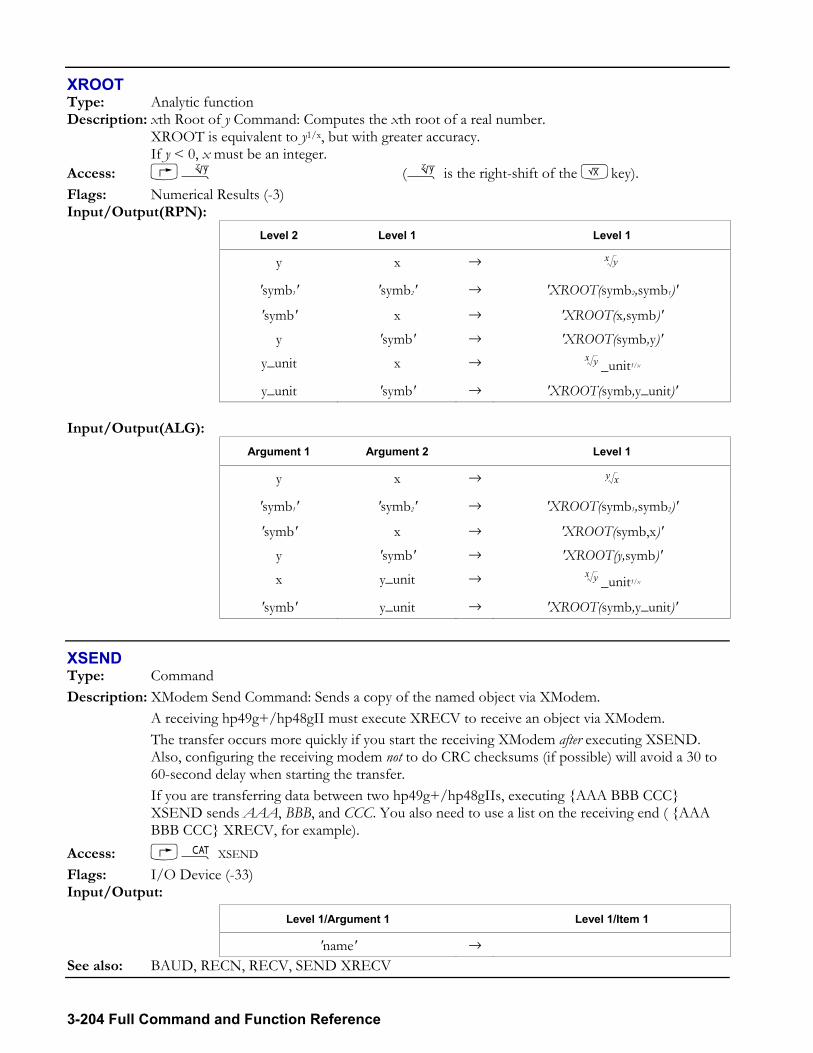
3-204 Full Command and Function Reference
XROOT Type: Analytic function Description: xth Root of y Command: Computes the xth root of a real number. XROOT is equivalent to y1/x, but with greater accuracy. If y < 0, x must be an integer. Access: » (» is the right-shift of the Rkey). Flags: Numerical Results (-3) Input/Output(RPN):
Level 2 Level 1 Level 1
y x → yx
'symb1' 'symb2' → 'XROOT(symb2,symb1)'
'symb' x → 'XROOT(x,symb)' y 'symb' → 'XROOT(symb,y)'
y_unit x → yx _unit1/x
y_unit 'symb' → 'XROOT(symb,y_unit)' Input/Output(ALG):
Argument 1 Argument 2 Level 1
y x → 'symb1' 'symb2' → 'XROOT(symb1,symb2)'
'symb' x → 'XROOT(symb,x)' y 'symb' → 'XROOT(y,symb)' x y_unit → yx _unit1/x
'symb' y_unit → 'XROOT(symb,y_unit)'
XSEND Type: Command Description: XModem Send Command: Sends a copy of the named object via XModem. A receiving hp49g+/hp48gII must execute XRECV to receive an object via XModem. The transfer occurs more quickly if you start the receiving XModem after executing XSEND.
Also, configuring the receiving modem not to do CRC checksums (if possible) will avoid a 30 to 60-second delay when starting the transfer.
If you are transferring data between two hp49g+/hp48gIIs, executing AAA BBB CCC XSEND sends AAA, BBB, and CCC. You also need to use a list on the receiving end ( AAA BBB CCC XRECV, for example).
Access: µ XSEND Flags: I/O Device (-33) Input/Output:
Level 1/Argument 1 Level 1/Item 1
'name' → See also: BAUD, RECN, RECV, SEND XRECV
x y
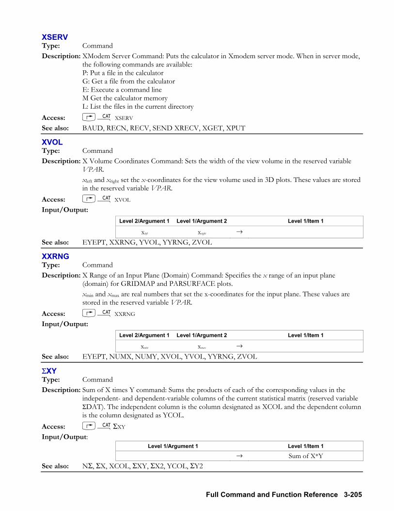
Full Command and Function Reference 3-205
XSERV Type: Command Description: XModem Server Command: Puts the calculator in Xmodem server mode. When in server mode,
the following commands are available: P: Put a file in the calculator G: Get a file from the calculator E: Execute a command line M Get the calculator memory L: List the files in the current directory
Access: µ XSERV See also: BAUD, RECN, RECV, SEND XRECV, XGET, XPUT
XVOL Type: Command Description: X Volume Coordinates Command: Sets the width of the view volume in the reserved variable
VPAR. xleft and xright set the x-coordinates for the view volume used in 3D plots. These values are stored
in the reserved variable VPAR. Access: µ XVOL Input/Output:
Level 2/Argument 1 Level 1/Argument 2 Level 1/Item 1
xleft xright → See also: EYEPT, XXRNG, YVOL, YYRNG, ZVOL
XXRNG Type: Command Description: X Range of an Input Plane (Domain) Command: Specifies the x range of an input plane
(domain) for GRIDMAP and PARSURFACE plots. xmin and xmax are real numbers that set the x-coordinates for the input plane. These values are
stored in the reserved variable VPAR. Access: µ XXRNG Input/Output:
Level 2/Argument 1 Level 1/Argument 2 Level 1/Item 1
xmin xmax → See also: EYEPT, NUMX, NUMY, XVOL, YVOL, YYRNG, ZVOL
ΣXY Type: Command Description: Sum of X times Y command: Sums the products of each of the corresponding values in the
independent- and dependent-variable columns of the current statistical matrix (reserved variable ΣDAT). The independent column is the column designated as XCOL and the dependent column is the column designated as YCOL.
Access: µΣXY Input/Output:
Level 1/Argument 1 Level 1/Item 1
→ Sum of X*Y See also: NΣ, ΣX, XCOL, ΣXY, ΣX2, YCOL, ΣY2
3-206 Full Command and Function Reference
ΣY Type: Command Description: Sum of y-Values Command: Sums the values in the dependent variable column of the current
statistical matrix (reserved variable ΣDAT). The dependent variable column is specified by YCOL, and is stored as the second parameter in
the reserved variable ΣPAR. The default dependent variable column number is 2. Access: µΣY Input/Output:
Level 1/Argument 1 Level 1/Item 1
→ Sum of Y See also: NΣ, ΣX, XCOL, ΣXY, ΣX2, YCOL, ΣY2
ΣY2 Type: Command Description: Sum of squares of Y-value command: Sums the squares of the values in the dependent-variable
columns of the current statistical matrix (reserved variable ΣDAT). The dependent column is the column designated as YCOL
Access: µΣY2 Input/Output:
Level 1/Argument 1 Level 1/Item 1
→ Sum of Y2
See also: NΣ, ΣX, XCOL, ΣXY, ΣX2, YCOL
YCOL Type: Command Description: Dependent Column Command: Specifies the dependent variable column of the current statistics
matrix (reserved variable ΣDAT). The dependent variable column number is stored as the second parameter in the reserved
variable ΣPAR. The default dependent variable column number is 2. YCOL will accept a noninteger real number and store it in ΣPAR, but subsequent commands
that utilize the YCOL specification in ΣPAR will cause an error. Access: µ YCOL Input/Output:
Level 1/Argument 1 Level 1/Item 1
ncol → See also: BARPLOT, BESTFIT, COLΣ, CORR, COV, EXPFIT, HISTPLOT, LINFIT, LOGFIT, LR,
PREDX, PREDY, PWRFIT, SCATRPLOT, XCOL
YRNG Type: Command Description: y-Axis Display Range Command: Specifies the y-axis display range. The y-axis display range is stored in the reserved variable PPAR as ymin and ymax in the complex
numbers (xmin, ymin) and (xmax, ymax). These complex numbers are the first two elements of PPAR and specify the coordinates of the lower left and upper right corners of the display ranges. The
Full Command and Function Reference 3-207
default values of ymin and ymax are 3.1 and 3.2, respectively for the hp48gII and -3.9 and 4.0, respectively for the hp49g+.
Access: µ YRNG Input/Output:
Level 2/Argument 1 Level 1/Argument 2 Level 1/Item 1
ymin ymax → See also: AUTO, PDIM, PMAX, PMIN, XRNG
YSLICE Type: Command Description: Y-Slice Plot Command: Sets the plot type to YSLICE. When plot type is set YSLICE, the DRAW command plots a slicing view of a scalar function of
two variables. YSLICE requires values in the reserved variables EQ, VPAR, and PPAR. VPAR has the following form: xleft, xright, ynear, yfar, zlow, zhigh, xmin, xmax, ymin, ymax, xeye, yeye, zeye, xstep, ystep For plot type YSLICE, the elements of VPAR are used as follows:
xleft and xright are real numbers that specify the width of the view space. ynear and yfar are real numbers that specify the depth of the view space. zlow and zhigh are real numbers that specify the height of the view space. xmin and xmax are not used. ymin and ymax are not used. xeye, yeye, and zeye are real numbers that specify the point in space from which the graph is
viewed. xstep determines the interval between plotted x-values within each slice. ystep determines the number of slices to draw.
The plotting parameters are specified in the reserved variable PPAR, which has this form: (xmin, ymin), (xmax, ymax), indep, res, axes, ptype, depend
For plot type YSLICE, the elements of PPAR are used as follows: (xmin, ymin) is not used. (xmax, ymax) is not used. indep is a name specifying the independent variable. The default value of indep is X. res is a real number specifying the interval, in user-unit coordinates, between plotted values of
the independent variable; or a binary integer specifying the interval in pixels. The default value is 0, which specifies an interval of 1 pixel.
axes is not used. ptype is a command name specifying the plot type. Executing the command YSLICE places
YSLICE in ptype. depend is a name specifying the dependent variable. The default value is Y.
Access: µ YSLICE Input/Output: None See also: BAR, CONIC, DIFFEQ, FUNCTION, GRIDMAP, HISTOGRAM, PARAMETRIC,
PARSURFACE, PCONTOUR, POLAR, SCATTER, SLOPEFIELD, TRUTH, WIREFRAME
YVOL Type: Command Description: Y Volume Coordinates Command: Sets the depth of the view volume in the reserved variable
VPAR.
3-208 Full Command and Function Reference
The variables ynear and yfar are real numbers that set the y-coordinates for the view volume used in 3D plots. ynear must be less than yfar. These values are stored in the reserved variable VPAR.
Access: µ YVOL Input/Output:
Level 2/Argument 1 Level 1/Argument 2 Level 1/Item 1
ynear yfar → See also: EYEPT, XVOL, XXRNG, YYRNG, ZVOL
YYRNG Type: Command Description: Y Range of an Input Plane (Domain) Command: Specifies the y range of an input plane
(domain) for GRIDMAP and PARSURFACE plots. The variables yy near and yy far are real numbers that set the y-coordinates for the input plane. These
values are stored in the reserved variable VPAR. Access: µ YYRNG Input/Output:
Level 2/Argument 1 Level 1/Argument 2 Level 1/Item 1
ynear yfar → See also: EYEPT, XVOL, XXRNG, YVOL, ZVOL
ZEROS CAS: Return the zeros of a function of one variable, without giving their multiplicity.
ZFACTOR Type: Function Description: Gas Compressibility Z Factor Function: Calculates the gas compressibility correction factor for
non-ideal behavior of a hydrocarbon gas. xTr is the reduced temperature: the ratio of the actual temperature (T) to the pseudocritical
temperature (Tc). (Calculate the ratio using absolute temperatures.) xTr must be between 1.05 and 3.0.
yPr is the reduced pressure: the ratio of the actual pressure (P) to the pseudocritical pressure (Pc). yPr must be between 0 and 30.
xTr and yPr must be real numbers or unit objects that reduce to dimensionless numbers. Access: µ ZFACTOR Flags: Numerical Results (-3) Input/Output:
Level 2/Argument 1 Level 1/Argument 2 Level 1/Item 1
xTr yPr → xZfactor
xTr 'symb' → 'ZFACTOR(xTr,symb)'
'symb' yPr → 'ZFACTOR(symb,yPr)'
'symb1' 'symb2' → 'ZFACTOR(symb1,symb2)'
ZVOL Type: Command
Full Command and Function Reference 3-209
Description: Z Volume Coordinates Command: Sets the height of the view volume in the reserved variable VPAR.
xlow and xhigh are real numbers that set the z-coordinates for the view volume used in 3D plots. These values are stored in the reserved variable VPAR.
Access: µ ZVOL Input/Output:
Level 2/Argument 1 Level 1/Argument 2 Level 1/Item 1
xlow xhigh → See also: EYEPT, XVOL, XXRNG, YVOL, YYRNG
^ (Power) Type: Function Description: Power Analytic Function: Returns the value of the level 2 object raised to the power of the level
1 object. This can also apply to a square matrix raised to a whole-number power. If either argument is complex, the result is complex. The branch cuts and inverse relations for wz are determined by this relationship:
wz = exp(z(ln w)) Access: Q
Flags: Principal Solution (-1), Numerical Results (-3) Input/Output:
Level 2/Argument 1 Level 1/Argument 2 Level 1/Item 1
w z → wz z 'symb' → 'z^(symb)'
'symb' z → '(symb)^z' 'symb1' 'symb2' → 'symb1^('symb2)' x_unit y → xy_unity x_unit 'symb' → '(x_unit)^(symb)'
See also: EXP, ISOL, LN, XROOT
| (Where) Type: Function Description: Where Function: Substitutes values for names in an expression. | is used primarily in algebraic objects, where its syntax is: 'symbold | (name1 = symb1, name2 = symb2 )' It enables algebraics to include variable-like substitution information about names. Symbolic
functions that delay name evaluation (such as ∫ and ∂) can then extract substitution information from local variables and include that information in the expression, avoiding the problem that would occur if the local variables no longer existed when the local names were finally evaluated.
Access: @¦ (¦is the right-shift of the Ikey). Flags: Numerical Results (-3) Input/Output:
Level 2/Argument 1 Level 1/Argument 2 Level 1/Item 1
'symbold' name1, 'symb1', name2, 'symb2' → 'symbnew'
x name1, 'symb1', name2, 'symb2' → x
(x,y) name1, 'symb1', name2, 'symb2' → (x,y)
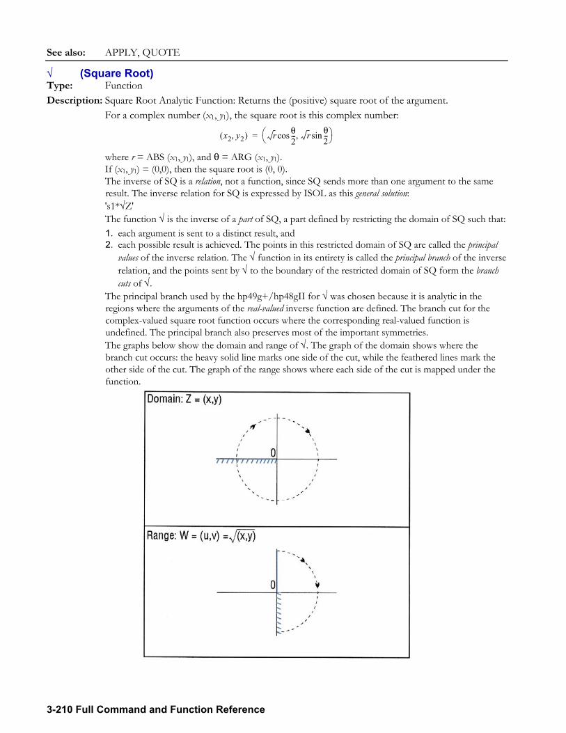
3-210 Full Command and Function Reference
See also: APPLY, QUOTE
√ (Square Root) Type: Function Description: Square Root Analytic Function: Returns the (positive) square root of the argument. For a complex number (x1, y1), the square root is this complex number:
x2 y2,( ) r θ2---
r,cos θ2---sin⎝ ⎠
⎛ ⎞=
where r = ABS (x1, y1), and θ = ARG (x1, y1). If (x1, y1) = (0,0), then the square root is (0, 0). The inverse of SQ is a relation, not a function, since SQ sends more than one argument to the same
result. The inverse relation for SQ is expressed by ISOL as this general solution: 's1*√Z' The function √ is the inverse of a part of SQ, a part defined by restricting the domain of SQ such that:
1. each argument is sent to a distinct result, and 2. each possible result is achieved. The points in this restricted domain of SQ are called the principal
values of the inverse relation. The √ function in its entirety is called the principal branch of the inverse relation, and the points sent by √ to the boundary of the restricted domain of SQ form the branch cuts of √.
The principal branch used by the hp49g+/hp48gII for √ was chosen because it is analytic in the regions where the arguments of the real-valued inverse function are defined. The branch cut for the complex-valued square root function occurs where the corresponding real-valued function is undefined. The principal branch also preserves most of the important symmetries.
The graphs below show the domain and range of √. The graph of the domain shows where the branch cut occurs: the heavy solid line marks one side of the cut, while the feathered lines mark the other side of the cut. The graph of the range shows where each side of the cut is mapped under the function.
Full Command and Function Reference 3-211
These graphs show the inverse relation 's1*√Z' for the case s1=1. For the other value of s1, the half-plane in the lower graph is rotated. Taken together, the half-planes cover the whole complex plane, which is the domain of SQ.
View these graphs with domain and range reversed to see how the domain of SQ is restricted to make an inverse function possible. Consider the half-plane in the lower graph as the restricted domain Z = (x, y). SQ sends this domain onto the whole complex plane in the range W = (u, v) = SQ(x, y) in the upper graph.
Access: R Flags: Principal Solution (-1), Numerical Results (-3) Input/Output:
Level 1/Argument 1 Level 1/Item 1
z → z x_unit → x unit1 2⁄
'symb' → ' symb( ) 'See also: SQ, ^, ISOL
∫ (Integrate) Type: Function Description: Integral Function: Integrates an integrand from lower limit to upper limit with respect to a specified
variable of integration. The algebraic syntax for ∫ parallels its stack syntax: ∫ (lower limit, upper limit, integrand, name) where lower limit, upper limit, and integrand can be real or complex numbers, unit objects, names, or
algebraic expressions. Evaluating ∫ in Symbolic Results mode (flag 3 clear) returns a symbolic result. Some functions
that the hp49g+/hp48gII can integrate include the following: All built-in functions whose antiderivatives can be expressed in terms of other built-in
functionsfor example, SIN can be integrated since its antiderivative, COS, is a built-in function. The arguments for these functions must be linear.
Sums, differences, and negations of built-in functions whose antiderivatives can be expressed in terms of other built-in functionsfor example, 'SIN(X)COS(X)'.
Derivatives of all built-in functionsfor example, 'INV(1+X^2)' can be integrated because it is the derivative of the built-in function ATAN.
Polynomials whose base term is linearfor example, 'X^3+X^22*X+6' can be integrated since X is a linear term. '(X^26)^3+(X^26)^2' cannot be integrated since X^26 is not linear.
Selected patterns composed of functions whose antiderivatives can be expressed in terms of other built-in functionsfor example, '1/(COS(X)*SIN(X))' returns 'LN(TAN(X))'.
If the result of the integration is an expression with no integral sign in the result, the symbolic integration was successful. If, however, the result still contains an integral sign, try rearranging the expression and evaluating again, or estimate the answer using numerical integration.
Evaluating ∫ in Numerical Results mode (flag 3 set) returns a numerical approximation, and stores the error of integration in variable IERR. ∫ consults the number format setting to determine how accurately to compute the result.
Access: Á (Á is the right-shift of the Ukey). Flags: Numerical Result (-3), Number Format (-45 to -50)
3-212 Full Command and Function Reference
Input/Output: L4/A1 L3/A2 L2/A3 L1/A4 L1/I1
lower limit upper limit integrand 'name' → 'symbintegral' L = Level; A = Argument; I = Item
See also: TAYLR, ∂, Σ
? (Undefined) CAS: The undefined symbol for numeric results that are not defined by the rules of arithmetic.
∞ (Infinity) CAS: Symbol signifies infinite numeric result, such as division of a non-zero number by zero.
Σ (Summation) Type: Function Description: Summation Function: Calculates the value of a finite series. The summand argument smnd can be a real number, a complex number, a unit object, a local or global
name, or an algebraic object. The algebraic syntax for Σ differs from the stack syntax. The algebraic syntax is: 'Σ(index=initial,final,summand)'
Access: ½ (½ is the right-shift of the Skey). Flags: Symbolic Constants (-2), Numerical Results (-3) Input/Output:
L4/A1 L3/A2 L2/A3 L1/A4 L1/I1
'indx' xinit xfinal smnd → xsum
'indx' 'init' xfinal smnd → 'Σ(indx = init, xfinal, smnd)'
'indx' xinit 'final' smnd → 'Σ(indx = xinit, final, smnd)'
'indx' 'init' 'final' smnd → 'Σ(indx = init, final, smnd)'L = Level; A = Argument; I = Item
See also: TAYLR, ∫, ∂
Σ+ (Sigma Plus) Type: Command Description: Sigma Plus Command: Adds one or more data points to the current statistics matrix (reserved
variable ΣDAT). For a statistics matrix with m columns, arguments for Σ+ can be entered several ways:
To enter one data point with a single coordinate value, the argument for Σ+ must be a real number.
To enter one data point with multiple coordinate values, the argument for Σ+ must be a vector with m real coordinate values.
To enter several data points, the argument for Σ+ must be a matrix of n rows of m real coordinate values.
In each case, the coordinate values of the data point(s) are added as new rows to the current statistics matrix (reserved variable ΣDAT). If ΣDAT does not exist, Σ+ creates an n x m matrix and stores the matrix in ΣDAT. If ΣDAT does exist, an error occurs if it does not contain a real matrix, or if the number of coordinate values in each data point entered with Σ+ does not match the number of columns in the current statistics matrix.
Once ΣDAT exists, individual data points of m coordinates can be entered as m separate real numbers or an m-element vector. LASTARG returns the m-element vector in either case.
Access: µΣ+
Full Command and Function Reference 3-213
Input/Output: Lm/A1 L2/Am1 L1/Am L1/I1
x →
[ x1, x2, , xm ] →
[[ x1 1, , x1 m ] [ xn 1, ,xn m ]] →
x1 xm1 xm → L = Level; A = Argument; I = Item
See also: CLΣ, RCLΣ, STOΣ, Σ
Σ (Sigma Minus) Type: Command Description: Sigma Minus Command: Returns a vector of m real numbers (or one number x if m = 1)
corresponding to the coordinate values of the last data point entered by Σ+ into the current statistics matrix (reserved variable ΣDAT).
The last row of the statistics matrix is deleted. The vector returned by Σ can be edited or replaced, then restored to the statistics matrix by Σ+. Access: µΣ Input/Output:
Level 1/Argument 1 Level 1/Item 1
→ x
→ [ x1 x2 xm ] See also: CLΣ, RCLΣ, STOΣ, Σ+
π (Pi) Type: Function Description: π Function: Returns the symbolic constant 'π' or its numerical representation, 3.14159265359. The number returned for π is the closest approximation of the constant π to 12-digit accuracy. In Radians mode with flag 2 and 3 clear (to return symbolic results), trigonometric functions
of π and π/2 are automatically simplified. For example, evaluating 'SIN(π)' returns zero. However, if flag 2 or flag 3 is set (to return numerical results), then evaluating 'SIN(π)' returns the numerical approximation 2.06761537357E13.
Access: !ì ( ìis the left-shift of the #key). Flags: Symbolic Constants (-2), Numerical Results (-3) Input/Output:
Level 1/Argument 1 Level 1/Item 1
→ 'π' → 3.14159265359
See also: e, i, MAXR, MINR, →Qπ
∂ (Derivative) Type: Function Description: Derivative Function: Takes the derivative of an expression, number, or unit object with respect
to a specified variable of differentiation.
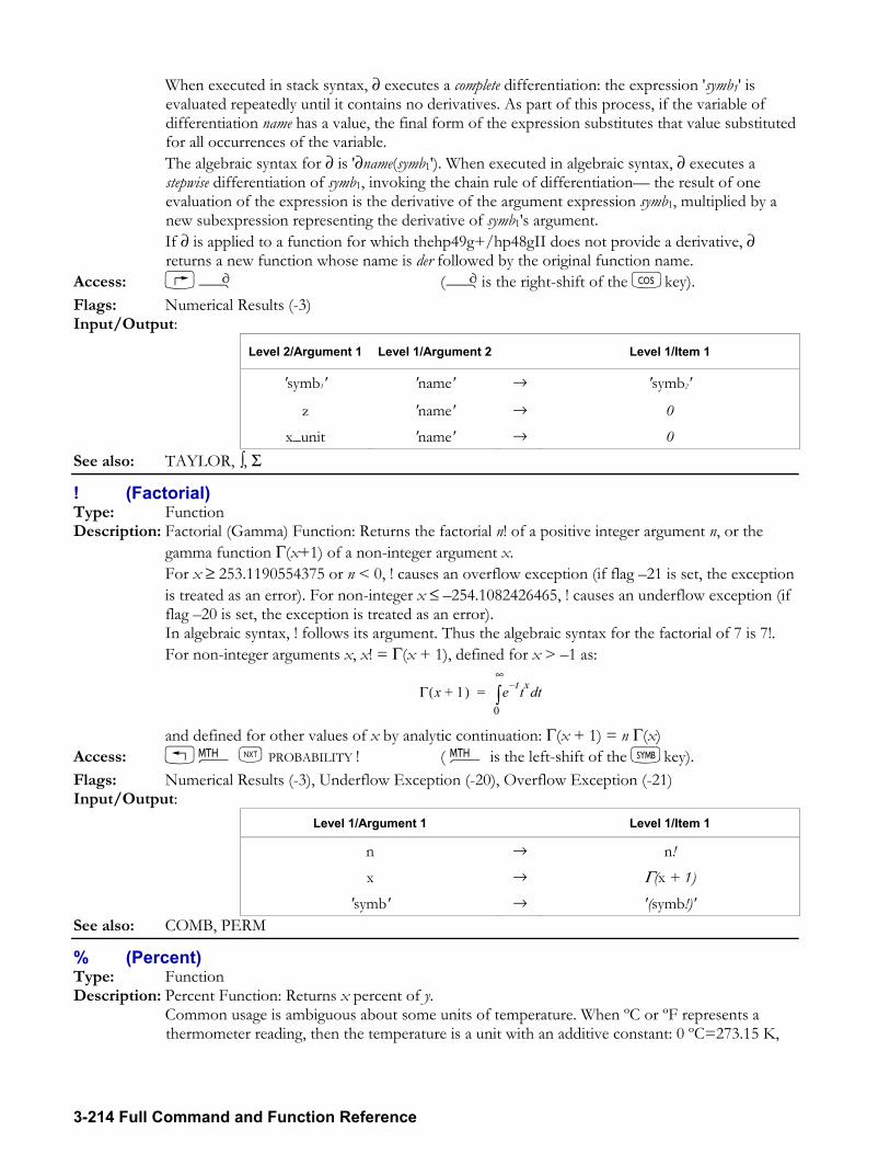
3-214 Full Command and Function Reference
When executed in stack syntax, ∂ executes a complete differentiation: the expression 'symb1' is evaluated repeatedly until it contains no derivatives. As part of this process, if the variable of differentiation name has a value, the final form of the expression substitutes that value substituted for all occurrences of the variable.
The algebraic syntax for ∂ is '∂name(symb1'). When executed in algebraic syntax, ∂ executes a stepwise differentiation of symb1, invoking the chain rule of differentiation the result of one evaluation of the expression is the derivative of the argument expression symb1, multiplied by a new subexpression representing the derivative of symb1's argument.
If ∂ is applied to a function for which thehp49g+/hp48gII does not provide a derivative, ∂ returns a new function whose name is der followed by the original function name.
Access: ¿ (¿is the right-shift of the Tkey). Flags: Numerical Results (-3) Input/Output:
Level 2/Argument 1 Level 1/Argument 2 Level 1/Item 1
'symb1' 'name' → 'symb2'
z 'name' → 0 x_unit 'name' → 0
See also: TAYLOR, ∫, Σ
! (Factorial) Type: Function Description: Factorial (Gamma) Function: Returns the factorial n! of a positive integer argument n, or the
gamma function Γ(x+1) of a non-integer argument x. For x ≥ 253.1190554375 or n < 0, ! causes an overflow exception (if flag 21 is set, the exception
is treated as an error). For non-integer x ≤ 254.1082426465, ! causes an underflow exception (if flag 20 is set, the exception is treated as an error).
In algebraic syntax, ! follows its argument. Thus the algebraic syntax for the factorial of 7 is 7!. For non-integer arguments x, x! = Γ(x + 1), defined for x > 1 as:
Γ x 1+( ) e t tx td0
∞
∫=
and defined for other values of x by analytic continuation: Γ(x + 1) = n Γ(x) Access: !´ L PROBABILITY ! ( ´ is the left-shift of the Pkey). Flags: Numerical Results (-3), Underflow Exception (-20), Overflow Exception (-21) Input/Output:
Level 1/Argument 1 Level 1/Item 1
n → n! x → Γ(x + 1)
'symb' → '(symb!)' See also: COMB, PERM
% (Percent) Type: Function Description: Percent Function: Returns x percent of y. Common usage is ambiguous about some units of temperature. When ºC or ºF represents a
thermometer reading, then the temperature is a unit with an additive constant: 0 ºC=273.15 K,
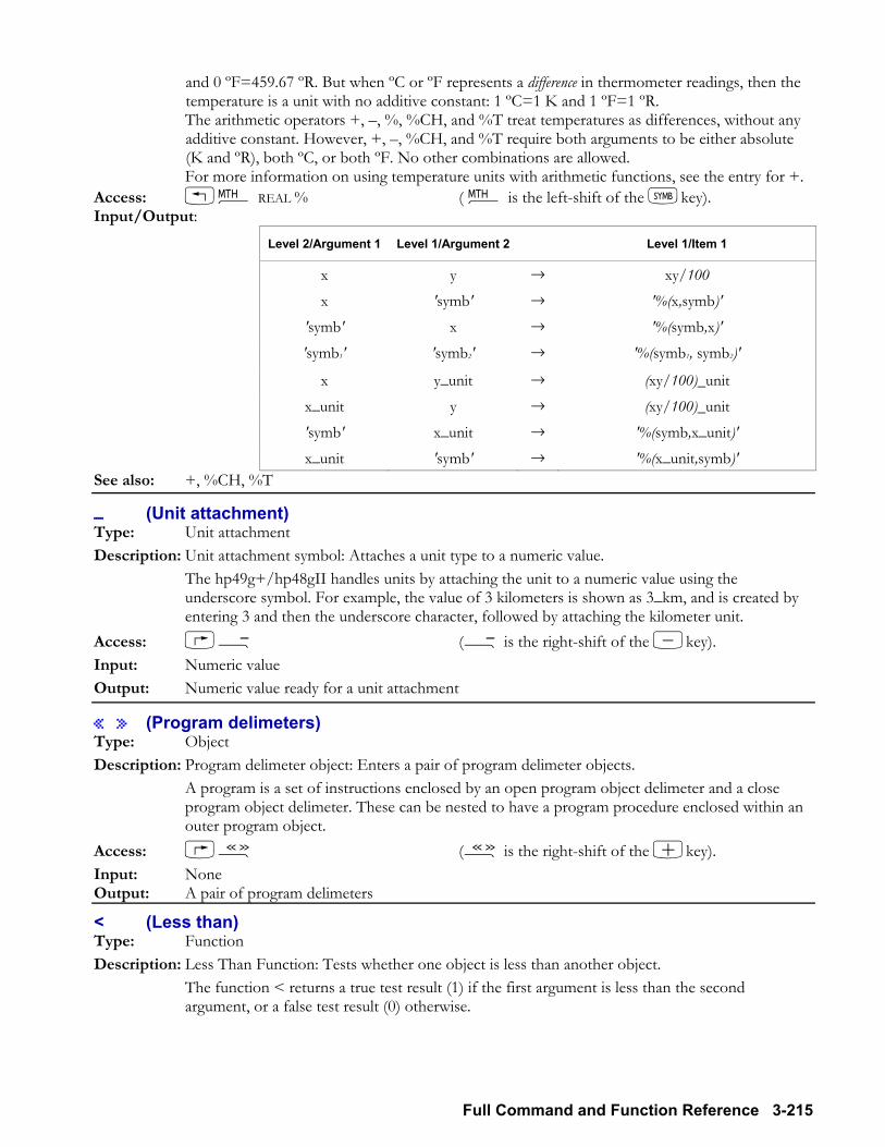
Full Command and Function Reference 3-215
and 0 ºF=459.67 ºR. But when ºC or ºF represents a difference in thermometer readings, then the temperature is a unit with no additive constant: 1 ºC=1 K and 1 ºF=1 ºR.
The arithmetic operators +, , %, %CH, and %T treat temperatures as differences, without any additive constant. However, +, , %CH, and %T require both arguments to be either absolute (K and ºR), both ºC, or both ºF. No other combinations are allowed.
For more information on using temperature units with arithmetic functions, see the entry for +. Access: !´ REAL % ( ´ is the left-shift of the Pkey). Input/Output:
Level 2/Argument 1 Level 1/Argument 2 Level 1/Item 1
x y → xy/100 x 'symb' → '%(x,symb)'
'symb' x → '%(symb,x)' 'symb1' 'symb2' → '%(symb1, symb2)'
x y_unit → (xy/100)_unit x_unit y → (xy/100)_unit 'symb' x_unit → '%(symb,x_unit)' x_unit 'symb' → '%(x_unit,symb)'
See also: +, %CH, %T
_ (Unit attachment) Type: Unit attachment Description: Unit attachment symbol: Attaches a unit type to a numeric value. The hp49g+/hp48gII handles units by attaching the unit to a numeric value using the
underscore symbol. For example, the value of 3 kilometers is shown as 3_km, and is created by entering 3 and then the underscore character, followed by attaching the kilometer unit.
Access: Ý (Ý is the right-shift of the -key). Input: Numeric value Output: Numeric value ready for a unit attachment
« » (Program delimeters) Type: Object Description: Program delimeter object: Enters a pair of program delimeter objects. A program is a set of instructions enclosed by an open program object delimeter and a close
program object delimeter. These can be nested to have a program procedure enclosed within an outer program object.
Access: å (å is the right-shift of the +key). Input: None Output: A pair of program delimeters
< (Less than) Type: Function Description: Less Than Function: Tests whether one object is less than another object. The function < returns a true test result (1) if the first argument is less than the second
argument, or a false test result (0) otherwise.
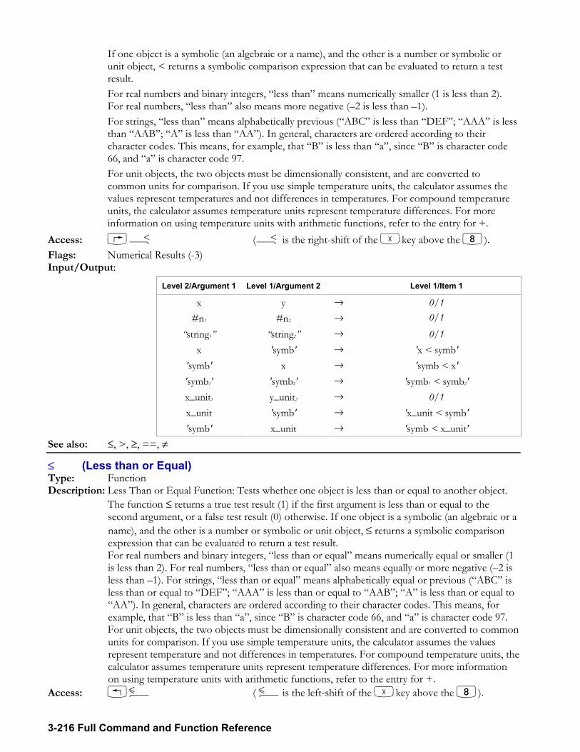
3-216 Full Command and Function Reference
If one object is a symbolic (an algebraic or a name), and the other is a number or symbolic or unit object, < returns a symbolic comparison expression that can be evaluated to return a test result.
For real numbers and binary integers, less than means numerically smaller (1 is less than 2). For real numbers, less than also means more negative (2 is less than 1).
For strings, less than means alphabetically previous (ABC is less than DEF; AAA is less than AAB; A is less than AA). In general, characters are ordered according to their character codes. This means, for example, that B is less than a, since B is character code 66, and a is character code 97.
For unit objects, the two objects must be dimensionally consistent, and are converted to common units for comparison. If you use simple temperature units, the calculator assumes the values represent temperatures and not differences in temperatures. For compound temperature units, the calculator assumes temperature units represent temperature differences. For more information on using temperature units with arithmetic functions, refer to the entry for +.
Access: Ç (Ç is the right-shift of the Xkey above the 8). Flags: Numerical Results (-3) Input/Output:
Level 2/Argument 1 Level 1/Argument 2 Level 1/Item 1
x y → 0/1 #n1 #n2 → 0/1
string1 string2 → 0/1 x 'symb' → 'x < symb'
'symb' x → 'symb < x' 'symb1' 'symb2' → 'symb1 < symb2' x_unit1 y_unit2 → 0/1 x_unit 'symb' → 'x_unit < symb' 'symb' x_unit → 'symb < x_unit'
See also: ≤, >, ≥, ==, ≠
≤ (Less than or Equal) Type: Function Description: Less Than or Equal Function: Tests whether one object is less than or equal to another object. The function ≤ returns a true test result (1) if the first argument is less than or equal to the
second argument, or a false test result (0) otherwise. If one object is a symbolic (an algebraic or a name), and the other is a number or symbolic or unit object, ≤ returns a symbolic comparison expression that can be evaluated to return a test result.
For real numbers and binary integers, less than or equal means numerically equal or smaller (1 is less than 2). For real numbers, less than or equal also means equally or more negative (2 is less than 1). For strings, less than or equal means alphabetically equal or previous (ABC is less than or equal to DEF; AAA is less than or equal to AAB; A is less than or equal to AA). In general, characters are ordered according to their character codes. This means, for example, that B is less than a, since B is character code 66, and a is character code 97.
For unit objects, the two objects must be dimensionally consistent and are converted to common units for comparison. If you use simple temperature units, the calculator assumes the values represent temperature and not differences in temperatures. For compound temperature units, the calculator assumes temperature units represent temperature differences. For more information on using temperature units with arithmetic functions, refer to the entry for +.
Access: !Æ ( Æis the left-shift of the Xkey above the 8).
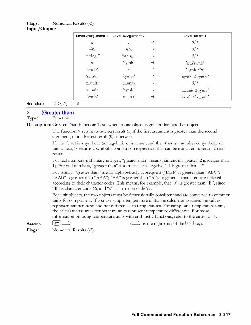
Full Command and Function Reference 3-217
Flags: Numerical Results (-3) Input/Output:
Level 2/Argument 1 Level 1/Argument 2 Level 1/Item 1
x y → 0/1 #n1 #n2 → 0/1
string1 string2 → 0/1 x 'symb' → 'x ≤ symb'
'symb' x → 'symb ≤ x' 'symb1' 'symb2' → 'symb1 ≤ symb2' x_unit1 y_unit2 → 0/1 x_unit 'symb' → 'x_unit ≤ symb' 'symb' x_unit → 'symb ≤ x_unit'
See also: <, >, ≥, ==, ≠
> (Greater than) Type: Function Description: Greater Than Function: Tests whether one object is greater than another object. The function > returns a true test result (1) if the first argument is greater than the second
argument, or a false test result (0) otherwise. If one object is a symbolic (an algebraic or a name), and the other is a number or symbolic or
unit object, > returns a symbolic comparison expression that can be evaluated to return a test result.
For real numbers and binary integers, greater than means numerically greater (2 is greater than 1). For real numbers, greater than also means less negative (1 is greater than 2).
For strings, greater than means alphabetically subsequent (DEF is greater than ABC; AAB is greater than AAA; AA is greater than A). In general, characters are ordered according to their character codes. This means, for example, that a is greater than B, since B is character code 66, and a is character code 97.
For unit objects, the two objects must be dimensionally consistent and are converted to common units for comparison. If you use simple temperature units, the calculator assumes the values represent temperatures and not differences in temperatures. For compound temperature units, the calculator assumes temperature units represent temperature differences. For more information on using temperature units with arithmetic functions, refer to the entry for +.
Access: É (É is the right-shift of the Ykey). Flags: Numerical Results (-3)
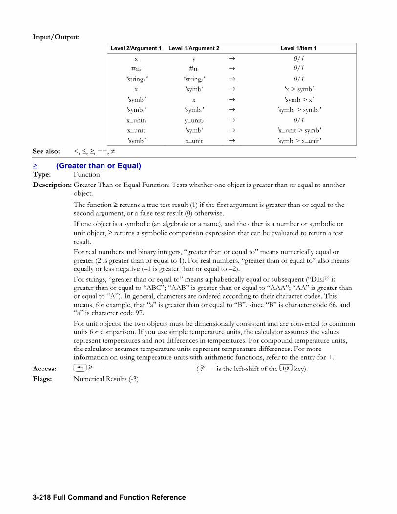
3-218 Full Command and Function Reference
Input/Output: Level 2/Argument 1 Level 1/Argument 2 Level 1/Item 1
x y → 0/1 #n1 #n2 → 0/1
string1 string2 → 0/1 x 'symb' → 'x > symb'
'symb' x → 'symb > x' 'symb1' 'symb2' → 'symb1 > symb2' x_unit1 y_unit2 → 0/1 x_unit 'symb' → 'x_unit > symb' 'symb' x_unit → 'symb > x_unit'
See also: <, ≤, ≥, ==, ≠
≥ (Greater than or Equal) Type: Function Description: Greater Than or Equal Function: Tests whether one object is greater than or equal to another
object. The function ≥ returns a true test result (1) if the first argument is greater than or equal to the
second argument, or a false test result (0) otherwise. If one object is a symbolic (an algebraic or a name), and the other is a number or symbolic or
unit object, ≥ returns a symbolic comparison expression that can be evaluated to return a test result.
For real numbers and binary integers, greater than or equal to means numerically equal or greater (2 is greater than or equal to 1). For real numbers, greater than or equal to also means equally or less negative (1 is greater than or equal to 2).
For strings, greater than or equal to means alphabetically equal or subsequent (DEF is greater than or equal to ABC; AAB is greater than or equal to AAA; AA is greater than or equal to A). In general, characters are ordered according to their character codes. This means, for example, that a is greater than or equal to B, since B is character code 66, and a is character code 97.
For unit objects, the two objects must be dimensionally consistent and are converted to common units for comparison. If you use simple temperature units, the calculator assumes the values represent temperatures and not differences in temperatures. For compound temperature units, the calculator assumes temperature units represent temperature differences. For more information on using temperature units with arithmetic functions, refer to the entry for +.
Access: !È ( Èis the left-shift of the Ykey). Flags: Numerical Results (-3)
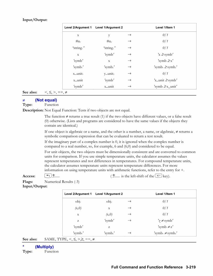
Full Command and Function Reference 3-219
Input/Output:
Level 2/Argument 1 Level 1/Argument 2 Level 1/Item 1
x y → 0/1 #n1 #n2 → 0/1
string1 string2 → 0/1
x 'symb' → 'x ≥ symb' 'symb' x → 'symb ≥ x' 'symb1' 'symb2' → 'symb1 ≥ symb2'
x_unit1 y_unit2 → 0/1
x_unit 'symb' → 'x_unit ≥ symb' 'symb' x_unit → 'symb ≥ x_unit'
See also: <, ≤, >, ==, ≠
≠ (Not equal) Type: Function Description: Not Equal Function: Tests if two objects are not equal. The function ≠ returns a true result (1) if the two objects have different values, or a false result
(0) otherwise. (Lists and programs are considered to have the same values if the objects they contain are identical.)
If one object is algebraic or a name, and the other is a number, a name, or algebraic, ≠ returns a symbolic comparison expression that can be evaluated to return a test result.
If the imaginary part of a complex number is 0, it is ignored when the complex number is compared to a real number, so, for example, 6 and (6,0) and considered to be equal.
For unit objects, the two objects must be dimensionally consistent and are converted to common units for comparison. If you use simple temperature units, the calculator assumes the values represent temperatures and not differences in temperatures. For compound temperature units, the calculator assumes temperature units represent temperature differences. For more information on using temperature units with arithmetic functions, refer to the entry for +.
Access: !Ä ( Äis the left-shift of the Wkey). Flags: Numerical Results (-3) Input/Output:
Level 2/Argument 1 Level 1/Argument 2 Level 1/Item 1
obj1 obj2 → 0/1
(x,0) x → 0/1 x (x,0) → 0/1 z 'symb' → 'z ≠ symb'
'symb' z 'symb ≠ z' 'symb1' 'symb2' → 'symb1 ≠ symb2'
See also: SAME, TYPE, <, ≤, >,≥, ==, ≠
* (Multiply) Type: Function
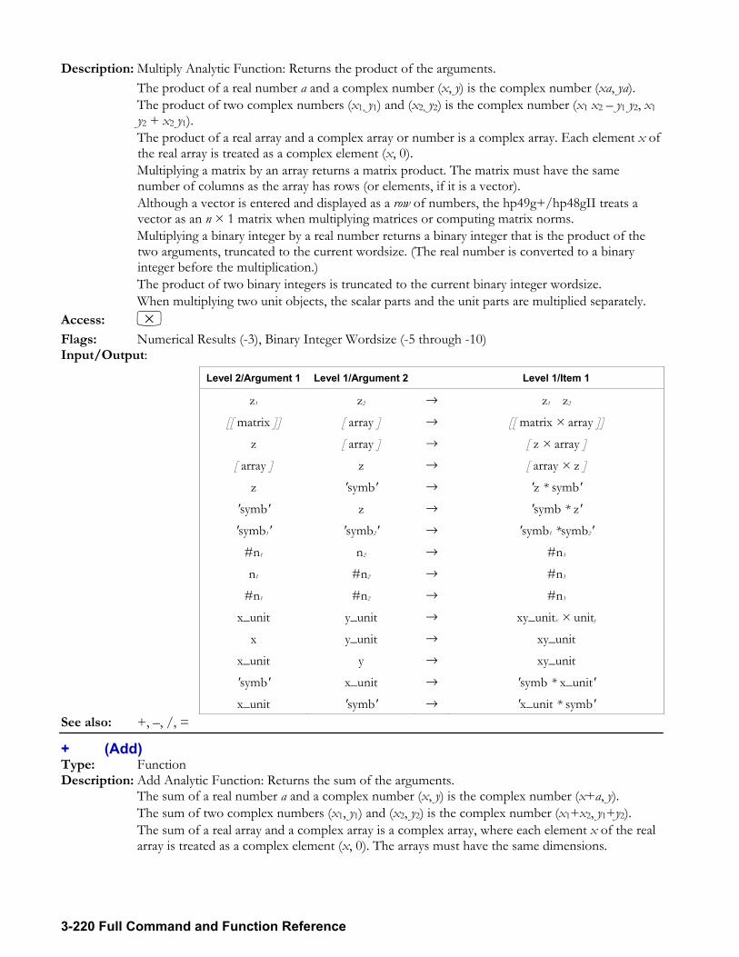
3-220 Full Command and Function Reference
Description: Multiply Analytic Function: Returns the product of the arguments. The product of a real number a and a complex number (x, y) is the complex number (xa, ya). The product of two complex numbers (x1, y1) and (x2, y2) is the complex number (x1 x2 y1 y2, x1
y2 + x2 y1). The product of a real array and a complex array or number is a complex array. Each element x of
the real array is treated as a complex element (x, 0). Multiplying a matrix by an array returns a matrix product. The matrix must have the same
number of columns as the array has rows (or elements, if it is a vector). Although a vector is entered and displayed as a row of numbers, the hp49g+/hp48gII treats a
vector as an n × 1 matrix when multiplying matrices or computing matrix norms. Multiplying a binary integer by a real number returns a binary integer that is the product of the
two arguments, truncated to the current wordsize. (The real number is converted to a binary integer before the multiplication.)
The product of two binary integers is truncated to the current binary integer wordsize. When multiplying two unit objects, the scalar parts and the unit parts are multiplied separately. Access: * Flags: Numerical Results (-3), Binary Integer Wordsize (-5 through -10) Input/Output:
Level 2/Argument 1 Level 1/Argument 2 Level 1/Item 1
z1 z2 → z1 z2 [[ matrix ]] [ array ] → [[ matrix × array ]]
z [ array ] → [ z × array ] [ array ] z → [ array × z ]
z 'symb' → 'z * symb' 'symb' z → 'symb * z' 'symb1' 'symb2' → 'symb1 *symb2'
#n1 n2 → #n3 n1 #n2 → #n3
#n1 #n2 → #n3 x_unit y_unit → xy_unitx × unity
x y_unit → xy_unit
x_unit y → xy_unit
'symb' x_unit → 'symb * x_unit' x_unit 'symb' → 'x_unit * symb'
See also: +, , /, =
+ (Add) Type: Function Description: Add Analytic Function: Returns the sum of the arguments. The sum of a real number a and a complex number (x, y) is the complex number (x+a, y). The sum of two complex numbers (x1, y1) and (x2, y2) is the complex number (x1+x2, y1+y2). The sum of a real array and a complex array is a complex array, where each element x of the real
array is treated as a complex element (x, 0). The arrays must have the same dimensions.
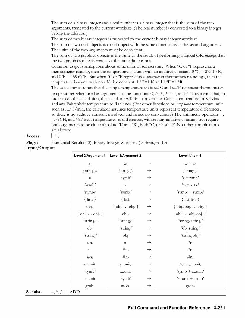
Full Command and Function Reference 3-221
The sum of a binary integer and a real number is a binary integer that is the sum of the two arguments, truncated to the current wordsize. (The real number is converted to a binary integer before the addition.)
The sum of two binary integers is truncated to the current binary integer wordsize. The sum of two unit objects is a unit object with the same dimensions as the second argument.
The units of the two arguments must be consistent. The sum of two graphics objects is the same as the result of performing a logical OR, except that
the two graphics objects must have the same dimensions. Common usage is ambiguous about some units of temperature. When ºC or ºF represents a
thermometer reading, then the temperature is a unit with an additive constant: 0 ºC = 273.15 K, and 0ºF = 459.67ºR. But when ºC or ºF represents a difference in thermometer readings, then the temperature is a unit with no additive constant: 1 ºC=1 K and 1 ºF =1 ºR.
The calculator assumes that the simple temperature units x_ºC and x_ºF represent thermometer temperatures when used as arguments to the functions <, >, ≤, ≥, ==, and ≠. This means that, in order to do the calculation, the calculator will first convert any Celsius temperature to Kelvins and any Fahrenheit temperature to Rankines. (For other functions or compound temperature units, such as x_ºC/min, the calculator assumes temperature units represent temperature differences, so there is no additive constant involved, and hence no conversion.) The arithmetic operators +, , %CH, and %T treat temperatures as differences, without any additive constant, but require both arguments to be either absolute (K and ºR), both ºC, or both ºF. No other combinations are allowed.
Access: +
Flags: Numerical Results (-3), Binary Integer Wordsize (-5 through -10) Input/Output:
Level 2/Argument 1 Level 1/Argument 2 Level 1/Item 1
z1 z2 → z1 + z2 [ array ]1 [ array ]2 → [ array ]3
z 'symb' → 'z +symb' 'symb' z → 'symb +z' 'symb1' 'symb2' → 'symb1 + symb2' list1 list2 → list1 list2
objA obj1 objn → objA obj1 objn obj1 objn objA → obj1 objn objA
string1 string2 → string1 string2 obj string → obj string
string obj → string obj #n1 n2 → #n3 n1 #n2 → #n3
#n1 #n2 → #n3 x1_unit1 y_unit2 → (x2 + y)_unit2 'symb' x_unit → 'symb + x_unit' x_unit 'symb' → 'x_unit + symb' grob1 grob2 → grob3
See also: , *, /, =, ADD
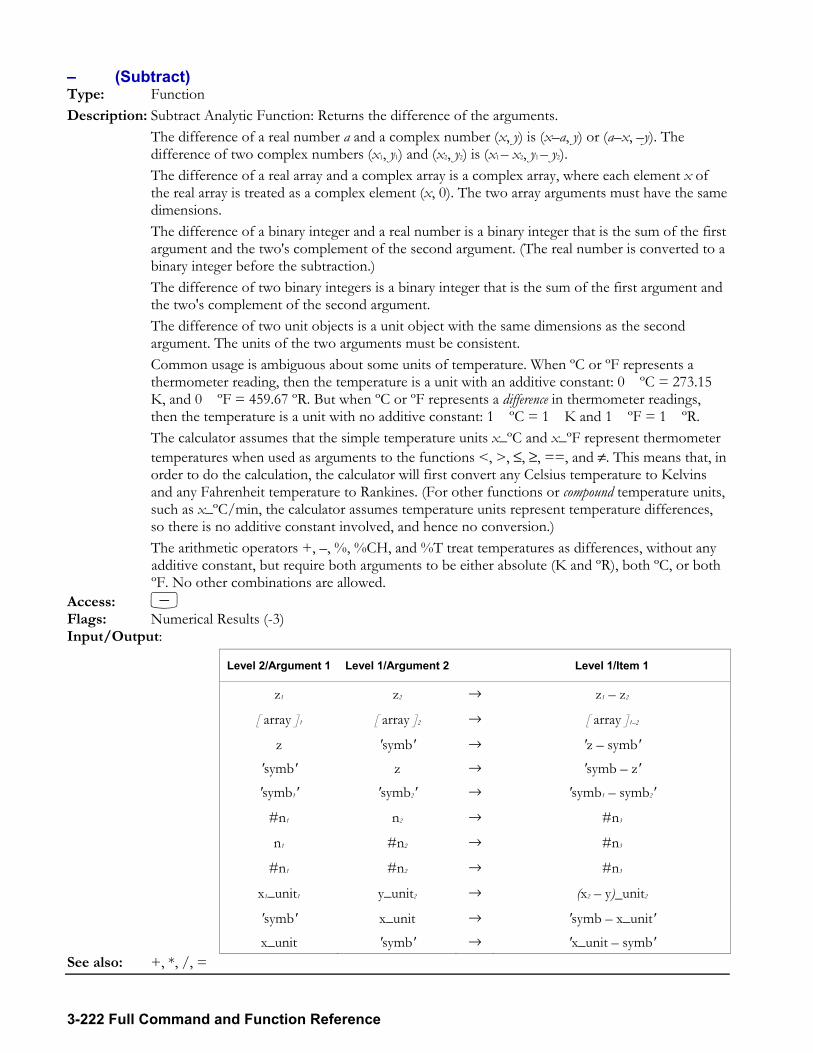
3-222 Full Command and Function Reference
(Subtract) Type: Function Description: Subtract Analytic Function: Returns the difference of the arguments. The difference of a real number a and a complex number (x, y) is (xa, y) or (ax, y). The
difference of two complex numbers (x1, y1) and (x2, y2) is (x1 x2, y1 y2). The difference of a real array and a complex array is a complex array, where each element x of
the real array is treated as a complex element (x, 0). The two array arguments must have the same dimensions.
The difference of a binary integer and a real number is a binary integer that is the sum of the first argument and the two's complement of the second argument. (The real number is converted to a binary integer before the subtraction.)
The difference of two binary integers is a binary integer that is the sum of the first argument and the two's complement of the second argument.
The difference of two unit objects is a unit object with the same dimensions as the second argument. The units of the two arguments must be consistent.
Common usage is ambiguous about some units of temperature. When ºC or ºF represents a thermometer reading, then the temperature is a unit with an additive constant: 0 ºC = 273.15 K, and 0 ºF = 459.67 ºR. But when ºC or ºF represents a difference in thermometer readings, then the temperature is a unit with no additive constant: 1 ºC = 1 K and 1 ºF = 1 ºR.
The calculator assumes that the simple temperature units x_ºC and x_ºF represent thermometer temperatures when used as arguments to the functions <, >, ≤, ≥, ==, and ≠. This means that, in order to do the calculation, the calculator will first convert any Celsius temperature to Kelvins and any Fahrenheit temperature to Rankines. (For other functions or compound temperature units, such as x_ºC/min, the calculator assumes temperature units represent temperature differences, so there is no additive constant involved, and hence no conversion.)
The arithmetic operators +, , %, %CH, and %T treat temperatures as differences, without any additive constant, but require both arguments to be either absolute (K and ºR), both ºC, or both ºF. No other combinations are allowed.
Access: - Flags: Numerical Results (-3) Input/Output:
Level 2/Argument 1 Level 1/Argument 2 Level 1/Item 1
z1 z2 → z1 z2
[ array ]1 [ array ]2 → [ array ]12
z 'symb' → 'z symb' 'symb' z → 'symb z' 'symb1' 'symb2' → 'symb1 symb2'
#n1 n2 → #n3
n1 #n2 → #n3
#n1 #n2 → #n3
x1_unit1 y_unit2 → (x2 y)_unit2
'symb' x_unit → 'symb x_unit' x_unit 'symb' → 'x_unit symb'
See also: +, *, /, =
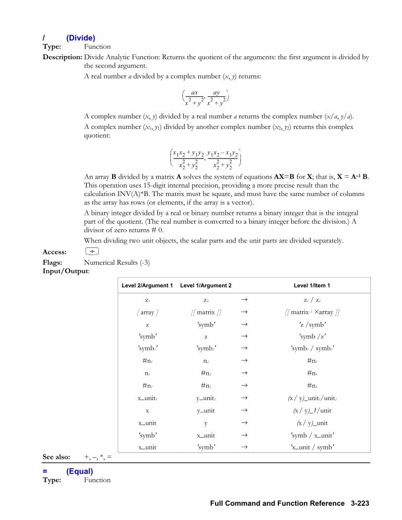
Full Command and Function Reference 3-223
/ (Divide) Type: Function Description: Divide Analytic Function: Returns the quotient of the arguments: the first argument is divided by
the second argument. A real number a divided by a complex number (x, y) returns:
ax
x2 y2+---------------- ay
x2 y2+----------------,⎝ ⎠
⎛ ⎞
A complex number (x, y) divided by a real number a returns the complex number (x/a, y/a). A complex number (x1, y1) divided by another complex number (x2, y2) returns this complex
quotient:
x1x2 y1y2+
x22 y2
2+----------------------------
y1x2 x1y2
x22 y2
2+---------------------------,
⎝ ⎠⎜ ⎟⎛ ⎞
An array B divided by a matrix A solves the system of equations AX=B for X; that is, X = A1 B.
This operation uses 15-digit internal precision, providing a more precise result than the calculation INV(A)*B. The matrix must be square, and must have the same number of columns as the array has rows (or elements, if the array is a vector).
A binary integer divided by a real or binary number returns a binary integer that is the integral part of the quotient. (The real number is converted to a binary integer before the division.) A divisor of zero returns # 0.
When dividing two unit objects, the scalar parts and the unit parts are divided separately. Access: / Flags: Numerical Results (-3) Input/Output:
Level 2/Argument 1 Level 1/Argument 2 Level 1/Item 1
z1 z2 → z1 / z2
[ array ] [[ matrix ]] → [[ matrix1 ×array ]]
z 'symb' → 'z /symb' 'symb' z → 'symb /z' 'symb1' 'symb2' → 'symb1 / symb2'
#n1 n2 → #n3
n1 #n2 → #n3
#n1 #n2 → #n3
x_unit1 y_unit2 → (x / y)_unit1/unit2
x y_unit → (x / y)_1/unit
x_unit y → (x / y)_unit
'symb' x_unit → 'symb / x_unit' x_unit 'symb' → 'x_unit / symb'
See also: +, , *, =
= (Equal) Type: Function
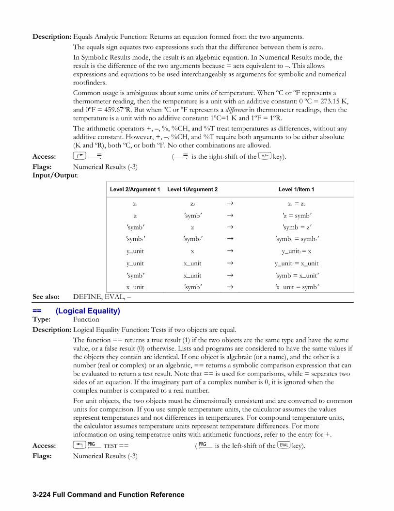
3-224 Full Command and Function Reference
Description: Equals Analytic Function: Returns an equation formed from the two arguments. The equals sign equates two expressions such that the difference between them is zero. In Symbolic Results mode, the result is an algebraic equation. In Numerical Results mode, the
result is the difference of the two arguments because = acts equivalent to . This allows expressions and equations to be used interchangeably as arguments for symbolic and numerical rootfinders.
Common usage is ambiguous about some units of temperature. When ºC or ºF represents a thermometer reading, then the temperature is a unit with an additive constant: 0 ºC = 273.15 K, and 0ºF = 459.67ºR. But when ºC or ºF represents a difference in thermometer readings, then the temperature is a unit with no additive constant: 1ºC=1 K and 1ºF = 1ºR.
The arithmetic operators +, , %, %CH, and %T treat temperatures as differences, without any additive constant. However, +, , %CH, and %T require both arguments to be either absolute (K and ºR), both ºC, or both ºF. No other combinations are allowed.
Access: Å (Å is the right-shift of the Wkey). Flags: Numerical Results (-3) Input/Output:
Level 2/Argument 1 Level 1/Argument 2 Level 1/Item 1
z1 z2 → z1 = z2
z 'symb' → 'z = symb' 'symb' z → 'symb = z' 'symb1' 'symb2' → 'symb1 = symb2'
y_unit x → y_unit1 = x
y_unit x_unit → y_unit1 = x_unit
'symb' x_unit → 'symb = x_unit' x_unit 'symb' → 'x_unit = symb'
See also: DEFINE, EVAL,
== (Logical Equality) Type: Function Description: Logical Equality Function: Tests if two objects are equal. The function == returns a true result (1) if the two objects are the same type and have the same
value, or a false result (0) otherwise. Lists and programs are considered to have the same values if the objects they contain are identical. If one object is algebraic (or a name), and the other is a number (real or complex) or an algebraic, == returns a symbolic comparison expression that can be evaluated to return a test result. Note that == is used for comparisons, while = separates two sides of an equation. If the imaginary part of a complex number is 0, it is ignored when the complex number is compared to a real number.
For unit objects, the two objects must be dimensionally consistent and are converted to common units for comparison. If you use simple temperature units, the calculator assumes the values represent temperatures and not differences in temperatures. For compound temperature units, the calculator assumes temperature units represent temperature differences. For more information on using temperature units with arithmetic functions, refer to the entry for +.
Access: !°TEST == ( °is the left-shift of the Nkey). Flags: Numerical Results (-3)
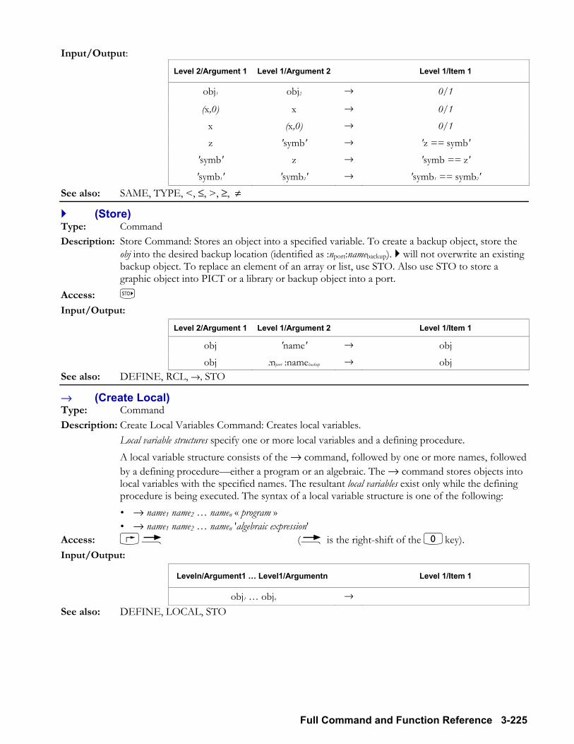
Full Command and Function Reference 3-225
Input/Output: Level 2/Argument 1 Level 1/Argument 2 Level 1/Item 1
obj1 obj2 → 0/1
(x,0) x → 0/1 x (x,0) → 0/1 z 'symb' → 'z == symb'
'symb' z → 'symb == z' 'symb1' 'symb2' → 'symb1 == symb2'
See also: SAME, TYPE, <, ≤, >, ≥, ≠
! (Store) Type: Command Description: Store Command: Stores an object into a specified variable. To create a backup object, store the
obj into the desired backup location (identified as :nport:namebackup). ! will not overwrite an existing backup object. To replace an element of an array or list, use STO. Also use STO to store a graphic object into PICT or a library or backup object into a port.
Access: K Input/Output:
Level 2/Argument 1 Level 1/Argument 2 Level 1/Item 1
obj 'name' → obj
obj :nport :namebackup → obj See also: DEFINE, RCL, →, STO
→ (Create Local) Type: Command Description: Create Local Variables Command: Creates local variables. Local variable structures specify one or more local variables and a defining procedure. A local variable structure consists of the → command, followed by one or more names, followed
by a defining procedureeither a program or an algebraic. The → command stores objects into local variables with the specified names. The resultant local variables exist only while the defining procedure is being executed. The syntax of a local variable structure is one of the following: → name1 name2 namen « program » → name1 name2 namen 'algebraic expression'
Access: é (é is the right-shift of the 0key). Input/Output:
Leveln/Argument1 Level1/Argumentn Level 1/Item 1
obj1 objn → See also: DEFINE, LOCAL, STO

4
Computer Algebra Commands 4-1
4.Computer Algebra Commands
Introduction The Computer Algebra System, or CAS, is a collection of operations that can be applied to algebraic expressions. The hp49g+/hp48gII operations can be used with numbers to produce numeric results, or with symbols to produce algebraic expressions. Algebraic expressions and equations can be written using the Equation Writer too. Algebraic expressions and symbolic operations on them, called computer algebra operations, are introduced in Chapter 5 of the Users Manual. Further explanations of computer algebra operations, are given in the Users Guide, whereas this part of the Advanced Users Guide lists the computer algebra operations that can be applied to symbolic expressions, with a description of each one listed. These operations perform tasks such as rearrangement of trigonometric and logarithmic functions, or manipulation of polynomials, series and matrices. They are referred to as the Computer Algebra System or the CAS. Many of the CAS operations are of particular use in Linear Algebra applications and in Vector Algebra. The CAS on the hp48gII and the hp49g+ allows these calculators to provide many of the features of the Computer Algebra Systems used on laptop and desktop computers. Note: The Computer Algebra System should not be confused with Algebraic mode, which is one of the calculators operating modes. The CAS works with algebraic (or symbolic) expressions, which can be entered and used in Algebraic mode or in RPN mode.
CAS Operations This volume of the Command Reference lists CAS operations, first according to the menus they appear in, then in detail, in alphabetic order. A few CAS operations appear in more than one menu. Some menus contain CAS operations and also operations that are not part of the CAS. Operations that are not part of the CAS are described in the full Command Reference in the previous chapter. For each CAS operation in the alphabetical list, some or all of the following details are provided: Type: Function or command. Functions, for example LCM, can be part of an algebraic expression.
Commands, for example SOLVE, cannot. When working with functions or commands within the Equation Writer: When you apply a function to an expression, the function becomes part of the expression.
You need to ensure that the expression is selected, then press Nto apply the function to the selection.
When you apply a command to an expression in Equation Writer, it is evaluated immediately.
Description: A description of the operation. Access: The menu or choose-list on which an operation can be found, and the keys that you press to
access it. If the operation is on a sub-menu, the sub-menu name is in SMALL CAPITALS after the keys. CAS commands that are not in any of the other menus on the keyboard can be accessed from the µ menu. Most CAS commands can also be accessed from the CASCMD choose-list, from CAS soft menus and from menus created by the MENUXY command.
4-2 Computer Algebra Commands
Input: The input argument or arguments that the operation needs. If the operation uses more than one input argument, details of the arguments and the order in which to supply them are provided: in argument order for algebraic mode and in stack order for RPN mode.
Output: The output that the operation produces. In RPN mode, the outputs are placed on the stack. In algebraic mode, the outputs are displayed; if there is more than one output, they are
written to a list. As with the input arguments, the outputs for both algebraic and RPN mode are described. Flags: Details of how flag settings affect the operation of the function or command. See also the
section below on CAS Settings. Example: An example of the function or command. Examples are also available in the built-in CAS help
on the calculator. The examples given here are shown in Algebraic mode, but can be transferred to RPN mode according to the descriptions given in Input and Output.
See also: Related functions or commands.
CAS Settings Selecting CAS Settings CAS settings are selected using the CAS MODES input form, described in Chapter 1 of the Users Manual. Selecting a mode is equivalent to setting or clearing one of the system flags, the flag numbers are given in the Flags part of the operation descriptions. Pressing the L key in the CAS MODES input form displays a menu that allows the user to calculate settings. For example, if the Modulo field is selected in the CAS MODES form, and L is pressed, the following menu keys are available. !TYPES lists the types of object that can be chosen for this setting. For the modulo, this can be a real number or an integer. For checked mode settings, this can only be a real number; if it is zero the mode is unchecked, if it is anything else the mode is checked. !CALC lets the user calculate a value for the setting, for example a new value for the modulo setting can be calculated. The !STS! menu key allows the user to switch the heading lines between the CAS MODES heading and the normal heading lines, so that the user can see what the current settings are while carrying out a calculation. !RESET allows the setting to be reset to its default value, or all CAS settings to be reset to their default values. See Appendix C in the Users Guide for further details of the CAS settings, and for other information about the CAS. Information on the Help system of the CAS is provided in Appendix C and also in Appendix H of the Users Guide. The CAS directory, CASDIR CAS settings are stored as flag settings, and as variables in the CASDIR directory, which is automatically created as a subdirectory of the HOME directory. Variables in this directory include: VX: A name or list of names of the current CAS variable or variables. Default value is X MODULO: The current modulus used for CAS modulo operations. Default value is 13, but is reset to 3
by the !RESET key in the CAS menu. PERIOD: The period for CAS periodic operations, 2π by default. EPS: The value chosen such that coefficients in a polynomial smaller than this value are replaced
with 0 by the EPSX0 command. 1E-10 by default. REALASSUME: A list of the names of variables that some CAS operations treat as real numbers when
complex mode is set. If additional assumptions are made on any variables, these are included here. By default the list is X, Y, t, S1, S2.
Computer Algebra Commands 4-3
PRIMIT: Temporary storage of anti-derivative expressions used during CAS operations. MATRIX: Temporary storage of a matrix used during CAS operations. CASINFO: Temporary storage of graphic display during step-by-step operations. PPAR: Plot parameters. Points to note when choosing settings The CAS is a powerful tool, and part of that power lies in the many modes and settings available. This means that if a setting is wrong then the CAS can give unexpected results or error messages. The following points should be observed. If an unexpected error occurs, or an unexpected message is seen, check this list.
• Many CAS commands will give numeric results instead of symbolic results if numeric mode is set instead of being cleared. Though these results may be correct, they will not be what the user wants if a symbolic result is needed. For this reason, the Flags section of most operation descriptions says that numeric mode should not be set.
• If approximate mode is set instead of exact mode, CAS commands will often give reasonable results, but unexpected results can be obtained, because, for example, powers are real numbers, not integers, for instance a cube will be treated as x3.0 instead of x3. For this reason, the Flags section of most operation descriptions says that exact mode should be set. Some commands, like the numeric solvers, will only find approximate solutions if approximate mode is set.
• CAS operations are designed to work with integers if possible, and some CAS operations round their inputs before using them. FIX 0 mode will round to whole numbers, losing accuracy. STD mode will retain full accuracy, so it is the best display mode to use with the CAS and is used in most of the examples in this chapter.
• For the same reasons, the general solutions, symbolic constants and symbolic arguments flags (flags 1, 2 and 3) should normally be clear when working with the CAS.
• Where possible, integer numbers should be used as input, not real numbers. The functions RND, CEIL and FLOOR can round a real number to a whole real number, and R$I will convert a whole real number to an integer.
• If complex inputs are given, approximate mode may need to be set to find solutions, and complex mode must be set (flag 103 set).
• Not only the trigonometry rewriting operations, but some other CAS operations require the angle mode to be set to radians (flag 17 clear), even if it is not immediately obvious that this is so. For this reason, the Flags section of many operation descriptions says that radians mode should be set.
• Some CAS operations will work one step at a time if step-by-step mode is set (flag 100 set). If a result is wanted immediately, and the calculator instead displays one step of the operation, cancel the operation, clear flag 100, then repeat the operation.
• If a mode needs to be changed for an operation to work, the calculator will by default ask if the mode can be changed. If the Silent mode switch flag (flag 120) is set, the calculator changes the mode without asking. If the mode switch disallowed flag (flag 123) is set, the mode will not be changed and an error will occur.
• All the system flags from 99 to 128 are intended for use by the CAS. It is worth reading Appendix C in the Users Guide to learn the detailed effects of these flags on CAS operations and displays.
• Remember that in RPN mode, symbolic expressions typed on the command line should be enclosed in single quote marks ′x + y′. For clarity, it can be helpful to type expressions in single quote marks in Algebraic mode too.
• It is important to write symbolic expressions using the current variable. Some CAS operations will work with this variable, but treat other variables simply as unknown numbers. If an expression has been entered using a variable other than the current variable, it may be simpler to change the current variable in the CAS MODES form, rather than rewrite the whole expression.
• In algebraic mode (flag 95 set), some CAS commands will replace variables with their numeric values before returning a result, even if argument to symbolic mode is set (flag 3 clear). In RPN mode,
4-4 Computer Algebra Commands
they will be returned as variables. Some other CAS commands will always replace variables with their numeric results.
• Because of the above, variables used in symbolic operations should not have the same names as variables stored in the current directory/folder (or in directories above this directory). If, for example, x is the current variable, and a variable called ′x′ exists in the current directory or in the HOME directory, then the value stored in ′x′ might be used instead of the symbolic variable x.
• The modulo value used in modulus calculations is 13 after the calculator is reset. If the CAS modes are reset with CASCFG, the modulo is also 13, but if the modes are reset using !RESET as above, the modulo is 3, otherwise it is the value most recently set. It is important to change this to the required value before carrying out any modulus operations.
Using the CAS Examples and Help In addition to the examples in this Command Reference, the built-in CAS help provides examples of CAS operations.
• If an operation is selected from the operations catalog, µ, and if help is available, then pressing the !HELP key shows help information. Pressing the %OK% menu key copies the operation to the command line, ready for use.
• If an operation is selected from the CASCMD list, IL CASCMD, the same help information is available, but instead of %OK%, there is an !ECHO key to copy the name and example to the command line. Evaluating the example and comparing it with the result shown in the help text is a quick way to check if the CAS settings are correct.
Compatibility with Other Calculators Some CAS operations replace similar operations that were available on older HP calculators. The older operation names have been kept on the hp48gII and the hp49g+ so that programs written for the older calculators will work on the new models without being rewritten. This means that some commands and functions have more than one name; the CAS names are in this part of the Command Reference, the older names are listed in Chapter 3. In other cases, operations that would naturally belong with the Computer Algebra System were already available on the older models; these operations too are described in Chapter 3. The older models whose programs can be run on the hp48gII and the hp49g+ are the HP 28C and HP 28S, the HP 48S and the HP 48SX, and the HP 48G, HP 48GX and HP 48G+. These models only had the RPL programming language, so programs written for them should be used in RPN mode. The HP 49G is a more recent model which does have the CAS, and Algebraic mode, so programs written for it in either RPL or in Algebraic mode can be used on the hp48gII and the hp49g+. The CAS of the hp48gII and the hp49g+ is also very similar to the CAS of the HP40 models, so programs and books written for them may be helpful. Extending the CAS Users can extend the CAS by writing their own functions or commands. Functions can be written as UDFs (User Defined Functions); see the descriptions of DEFINE in Chapter 3 of the calculator Users Guide and in Part A of this Command Reference, and also DEF in this part. The pattern matching commands ↑MATCH and ↓MATCH allow the user to write programs to edit algebraic expressions. Here is an example of an RPL program using ↑MATCH to replace the square root of a square of a symbol with the symbol itself. The wildcard &A means that any symbol or expression squared can be replaced. The conditional expression &A≥0 means that the replacement is only carried out if the square root is not of a negative value.
« '√(&A^2)' &A '&A≥0' ↑MATCH » Dealing with unexpected CAS results or messages If a CAS operation gives an unexpected result or message, check the list of points given in the section on CAS settings. Some problems can be caused by unexpected settings, so it can be helpful to reset all CAS settings to their default values, with the CASCFG command, or with the !RESET key in the CAS settings menu.
Computer Algebra Commands 4-5
Computer algebra command categories listed by menu CAS operations are listed here in order of the keyboard menus they appear in. These menus can be selected from the CAS menu in G, or directly from the keyboard. Many CAS commands are also available from the P menu, or from the ´ menu; these menus are not listed here, to avoid duplication. The CAS has its own menu commands too, they are included in the alphabetical list of commands. Operations that do not appear in any menu can be spelled out or selected from µ. Algebra commands, × COLLECT .......................... 4-19 EXPAND .......................... 4-29 FACTOR .......................... 4-30 LIN .......................... 4-48 LNCOLLECT ......................... 4-49 PARTFRAC .......................... 4-56 SOLVE .......................... 4-67 SUBST .......................... 4-69 TEXPAND .......................... 4-74 Arithmetic commands Arithmetic Integer commands, !ÞINTEGER EULER .......................... 4-28 IABCUV .......................... 4-38 IBERNOULLI ......................... 4-39 ICHINREM .......................... 4-40 IDIV2 .......................... 4-40 IEGCD .......................... 4-40 IQUOT .......................... 4-43 IREMAINDER........................ 4-43 ISPRIME? .......................... 4-44 NEXTPRIME .......................... 4-55 PA2B2 .......................... 4-55 PREVPRIME .......................... 4-59 Arithmetic Polynomial commands, !ÞPOLYNOMIAL ABCUV .......................... 4-12 CHINREM .......................... 4-17 CYCLOTOMIC ....................... 4-20 DIV2 .......................... 4-23 EGCD .......................... 4-27 FACTOR .......................... 4-30 FCOEF .......................... 4-31 FROOTS .......................... 4-33 GCD .......................... 4-34 HERMITE .......................... 4-37
4-6 Computer Algebra Commands
HORNER .......................... 4-38 LAGRANGE .......................... 4-45 LCM .......................... 4-46 LEGENDRE .......................... 4-47 PARTFRAC .......................... 4-56 PTAYL .......................... 4-59 QUOT .......................... 4-60 REMAINDER ......................... 4-61 RESULTANT .......................... 4-62 STURM .......................... 4-69 STURMAB .......................... 4-69 Other POLYNOMIAL operations are described in Chapter 3. Arithmetic Modulo commands, !ÞMODULO ADDTMOD .......................... 4-12 DIV2MOD .......................... 4-24 DIVMOD .......................... 4-25 EXPANDMOD....................... 4-30 FACTORMOD........................ 4-31 GCDMOD .......................... 4-35 INVMOD .......................... 4-42 MODSTO .......................... 4-53 MULTMOD .......................... 4-54 POWMOD .......................... 4-58 SUBTMOD .......................... 4-70 Other MODULO operations are described in Chapter 3. Arithmetic Permutation commands, !ÞPERMUTATION C2P .......................... 4-17 CIRC .......................... 4-18 P2C .......................... 4-55 Other Arithmetic commands, !Þ DIVIS .......................... 4-24 FACTORS .......................... 4-31 LGCD .......................... 4-48 PROPFRAC .......................... 4-59 SIMP2 .......................... 4-66 Calculus commands Derivation and integration commands, !ÖDERIV. & INTEG. CURL .......................... 4-19 DERIV .......................... 4-21 DERVX .......................... 4-21 DIV .......................... 4-23 FOURIER .......................... 4-32 HESS .......................... 4-37
Computer Algebra Commands 4-7
IBP .......................... 4-39 INTVX .......................... 4-42 LAPL .......................... 4-46 PREVAL .......................... 4-58 RISCH .......................... 4-62 SIGMA .......................... 4-65 SIGMAVX .......................... 4-65 Limits and series commands, !ÖLIMITS & SERIES DIVPC .......................... 4-25 lim .......................... 4-48 SERIES .......................... 4-64 TAYLOR0 .......................... 4-73 Other LIMITS & SERIES operations are described in Chapter 3. Differential equations commands, !ÖDIFFERENTIAL EQNS DESOLVE .......................... 4-22 ILAP .......................... 4-41 LAP .......................... 4-45 LDEC .......................... 4-47 Graphing commands, !ÖGRAPH SIGNTAB .......................... 4-65 TABVAL .......................... 4-71 TABVAR .......................... 4-71 Other GRAPH operations are described in Chapter 3. Other Calculus commands, !Ö DERVX .......................... 4-21 INTVX .......................... 4-42 These two operations are available directly from the CALC menu as well as being in the Derivation and Integration commands menu.
Exp and Lin commands, !Ð
EXPLN .......................... 4-30 LIN .......................... 4-48 LNCOLLECT .......................... 4-49 TEXPAND .......................... 4-74 TSIMP .......................... 4-77 Other EXP & LN operations are described in Chapter 3. Matrix-related commands Create, !Ø CREATE AUGMENT .......................... 4-15 HILBERT .......................... 4-37 VANDERMONDE ................ 4-78
4-8 Computer Algebra Commands
Other CREATE operations are described in Chapter 3. Operations, !Ø OPERATIONS AXL .......................... 4-15 AXM .......................... 4-16 HADAMARD .......................... 4-36 MAD .......................... 4-51 Other operations in the OPERATIONS submenu are described Chapter 3. All operations in the FACTORIZATION submenu are described Chapter 3. Quadratic form, !Ø QUADRATIC FORM AXQ .......................... 4-16 CHOLESKY .......................... 4-18 GAUSS .......................... 4-33 QXA .......................... 4-60 SYLVESTER .......................... 4-70 Linear Systems, !Ø LINEAR SYSTEMS LINSOLVE .......................... 4-49 REF .......................... 4-60 RREF .......................... 4-62 rref .......................... 4-63 SYST2MAT .......................... 4-71 Linear Applications, !Ø LINEAR APPL IMAGE .......................... 4-41 ISOM .......................... 4-43 KER .......................... 4-45 MKISOM .......................... 4-53 Eigenvectors, !Ø EIGENVECTORS DIAGMAP .......................... 4-22 JORDAN .......................... 4-44 PCAR .......................... 4-56 PMINI .......................... 4-56 Other operations in the EIGENVECTORS submenu are described in Chapter 3. Vector, !Ø VECTOR BASIS .......................... 4-16 GRAMSCHMIDT................... 4-35 IBASIS .......................... 4-38 Other operations in the VECTOR submenu are described in Chapter 3.
Symbolic solve commands, !Î DESOLVE .......................... 4-22 LDEC .......................... 4-47 LINSOLVE .......................... 4-49 SOLVEVX .......................... 4-68
Computer Algebra Commands 4-9
SOLVE .......................... 4-67 ZEROS .......................... 4-80 Other S.SLV operations are described in Chapter 3. Trigonometry commands, Ñ
All operations in the HYPERBOLIC submenu are described in Chapter 3. ACOS2S .......................... 4-12 ASIN2C .......................... 4-14 ASIN2T .......................... 4-14 ATAN2S .......................... 4-15 HALFTAN .......................... 4-36 SINCOS .......................... 4-67 TAN2SC .......................... 4-72 TAN2SC2 .......................... 4-73 TCOLLECT .......................... 4-74 TEXPAND .......................... 4-74 TLIN .......................... 4-74 TRIG .......................... 4-75 TRIGCOS .......................... 4-75 TRIGSIN .......................... 4-76 TRIGTAN .......................... 4-76 TSIMP ....................................... 4-77 Convert commands, !Ú
All operations in the UNITS and BASE submenus are described in Chapter 3. Trigonometric conversions, !Ú TRIG CONV ACOS2S .......................... 4-12 ASIN2C .......................... 4-14 ASIN2T .......................... 4-14 ATAN2S .......................... 4-15 HALFTAN .......................... 4-36 SINCOS .......................... 4-67 TAN2SC .......................... 4-72 TAN2SC2 .......................... 4-73 TLIN .......................... 4-74 TRIG .......................... 4-75 TRIGCOS .......................... 4-75 TRIGSIN .......................... 4-76 TSIMP .......................... 4-77 Rewrite expression, !Ú REWRITE DISTRIB .......................... 4-23 EXP2POW .......................... 4-29
4-10 Computer Algebra Commands
EXPLN .......................... 4-30 FDISTRIB .......................... 4-32 LIN .......................... 4-48 LNCOLLECT .......................... 4-49 POWEXPAND ....................... 4-57 SIMPLIFY .......................... 4-66 Other operations in the REWRITE submenu are described in Chapter 3. Matrix convert, !Ú MATRIX CONVERT AXL .......................... 4-15 AXQ .......................... 4-16 QXA .......................... 4-60 SYST2MAT .......................... 4-71 Other CAS operations, µ
These operations are in other menus, as described in Access for each one, or can be accessed with µ. Other mathematics operations DEGREE .......................... 4-21 DOMAIN .......................... 4-25 DROITE .......................... 4-26 dn .......................... 4-26 EPSX0 .......................... 4-27 EXLR .......................... 4-28 EXP2HYP .......................... 4-28 FXND .......................... 4-33 GBASIS .......................... 4-34 GREDUCE .......................... 4-35 LCXM .......................... 4-46 LIMIT .......................... 4-48 LNAME .......................... 4-49 LVAR .......................... 4-50 MSLV .......................... 4-54 P2C .......................... 4-55 POTENTIAL .......................... 4-57 REORDER .......................... 4-61 RREFMOD .......................... 4-63 SEVAL .......................... 4-64 TAN2CS2 .......................... 4-72 TCHEBYCHEFF ................... 4-73 TRUNC .......................... 4-77 VPOTENTIAL........................ 4-79 XNUM .......................... 4-80
Computer Algebra Commands 4-11
XQ .......................... 4-80 ? .......................... 4-81 ∞ .......................... 4-81 CAS menu commands, µ These commands display menus or lists of CAS operations. ALGB .......................... 4-13 ARIT .......................... 4-13 CONSTANTS .......................... 4-19 DIFF .......................... 4-23 EXP&LN .......................... 4-28 INTEGER .......................... 4-42 MAIN .......................... 4-51 MATHS .......................... 4-51 MATR .......................... 4-52 MENUXY .......................... 4-52 MODULAR .......................... 4-53 POLYNOMIAL....................... 4-57 REWRITE .......................... 4-62 TESTS .......................... 4-74 TRIGO .......................... 4-76 CAS utility operations ADDTOREAL......................... 4-13 ASSUME .......................... 4-14 CASCFG .......................... 4-17 CASCMD .......................... 4-17 DEDICACE .......................... 4-20 DEF .......................... 4-20 HELP .......................... 4-36 LOCAL .......................... 4-50 RCLVX .......................... 4-60 STORE .......................... 4-68 STOVX .......................... 4-68 UNASSIGN .......................... 4-77 UNASSUME .......................... 4-78 UNBIND .......................... 4-78 VER .......................... 4-79
4-12 Computer Algebra Commands
Alphabetical command list The following pages contain the commands in alphabetical order. See "Computer algebra command categories" on page 4-5 to view the commands in the order that they appear on the menus. Chapters 11 to 16 in the Users Guide provide examples using many of these commands. ABCUV Type: Command Description: Returns a solution in polynomials u and v of au+bv =c where a and b are polynomials in the
current CAS independent variable, and c is a value.
Access: Arithmetic, !Þ POLYNOMIAL Input: Level 3/Argument 1: The polynomial corresponding to a.
Level 2/Argument 2: The polynomial corresponding to b. Level 1/Argument 3: The value corresponding to c.
Output: Level 2/Item 1: The solution corresponding to u. Level 1/Item 2: The solution corresponding to v.
Flags: Exact mode must be set (flag 105 clear). Numeric mode must not be set (flag 3 clear). Radians mode must be set (flag 17 set).
Example: Find a solution in polynomials u and v for the following equation: x2 x 1+ +( )u x2 4+( )V+ 13=
Command: ABCUV(X^2+X+1,X^2+4,13)
Result: -(X+3),X+4
See also: IABCUV, EGCD
ACOS2S Type: Command Description: Transforms an expression by replacing acos(x) in subexpressions with π/2asin(x).
Access: Trigonometry, Ñ
Input: The expression to transform. Output: The transformed expression. Flags: Exact mode must be set (flag 105 clear).
Numeric mode must not be set (flag 3 clear). Radians mode must be set (flag 17 set).
Example: Simplify the following expression:
arc 2
3---⎝ ⎠⎛ ⎞cos arc x( )cos+
Command: ACOS2S(ACOS(2/3)+ACOS(X))
Result: π/2-ASIN(2/3)+π/2-ASIN(X)
See also: ASIN2C, ASIN2T, ATAN2S
ADDTMOD Type: Function Description: Adds two expressions or values, modulo the current modulus.
Computer Algebra Commands 4-13
Access: Arithmetic, !Þ MODULO Input: Level 2/Argument 1: The first expression.
Level 1/Argument 2: The second expression. Output: The sum of the two expressions, modulo the current modulus. Flags: Exact mode must be set (flag 105 clear).
Numeric mode must not be set (flag 3 clear). Radians mode must be set (flag 17 set).
Example: Express the result of the following addition in modulo 7. (x2+3x+6)+(9x+3) Note: Before trying this example, use the CAS modes input form to set the modulo to 7.
Command: ADDTMOD(X^2+3*X+6,9*X+3)
Result: X^2-2*X+2
ADDTOREAL Type: Command Description: Adds specified global names to the reserved variable REALASSUME. This is a list of the
global variables that will be treated by some CAS operations as real numbers when Complex mode is set. If a variable is already in the REALASSSUME list, this command removes any additional assumptions made on it by ASSUME.
Access: Catalog, µ Input: Level 1/Item 1: The name of the global variable to be added to the REALASSUME list, or a
list of names. Output: No output in RPN mode, NOVAL in Algebraic mode. Flags: If the all variables are real flag is set (flag 128 set), ADDTOREAL will not add anything to
the REALASSUME list, as all variables are assumed real anyway. In this case it will only remove further assumptions made by ASSUME.
See also: ASSUME, DEF, STORE, UNASSUME, UNBIND
ALGB Type: Command Description: Displays a menu or list of CAS algebraic operations.
Access: Catalog, µ Flags: If the CHOOSE boxes flag is clear (flag 117 clear), displays the operations as a numbered
list. If the flag is set, displays the operations as a menu of function keys. See also: ARIT, CONSTANTS, DIFF, EXP&LN, INTEGER, MAIN, MATHS, MATR, MODULAR,
POLYNOMIAL, REWRITE, TESTS, TRIGO
ARIT Type: Command Description: Displays a menu or list showing the three CAS submenus for arithmetical operations,
INTEGER, MODULAR and POLYNOMIAL.
Access: Catalog, µ Flags: If the CHOOSE boxes flag is clear (flag 117 clear), displays the submenus as a numbered
list. If the flag is set, displays the operations as a menu of function keys.
4-14 Computer Algebra Commands
See also: ALGB, CONSTANTS, DIFF, EXP&LN, INTEGER, MAIN, MATHS, MATR, MODULAR, POLYNOMIAL, REWRITE, TESTS, TRIGO
ASIN2C Type: Command Description: Transforms an expression by replacing asin(x) subexpressions with π/2acos(x)
subexpressions.
Access: Trigonometry, Ñ
Input: An expression Output: The transformed expression. Flags: Exact mode must be set (flag 105 clear).
Numeric mode must not be set (flag 3 clear). Radians mode must be set (flag 17 set).
See also: ACOS2S, ASIN2T, ATAN2S
ASIN2T Type: Command Description: Transforms an expression by replacing asin(x) subexpressions with the following:
x
1 x2------------------⎝ ⎠⎜ ⎟⎛ ⎞
atan
Access: Trigonometry, Ñ
Input: An expression. Output: The transformed expression. Flags: Exact mode must be set (flag 105 clear).
Numeric mode must not be set (flag 3 clear). Radians mode must be set (flag 17 set).
See also: ASIN2C, ACOS2S, ATAN2S
ASSUME Type: Function Description: Adds global names to the reserved variable REALASSUME, with specific assumptions.
REALASSUME is a list of the global variables that will be considered by some CAS operations to represent real numbers when complex mode is set. ASSUME adds further assumptions, for example that a variable is greater than or equal to zero. Assumptions must be of the form v≤expression, or v≥expression, where v is the variable name. Several assumptions can be combined. These assumptions are used by the solve commands; for example if a variable is assumed to be greater than zero then the solvers will not look for solutions where that variable is negative. Some of the solvers will give complex solutions for variables even if they are in REALASSUME.
Access: Catalog, µ Input: Level 1/Item 1: An expression giving the name of the global variable to be added to the
REALASSUME list, and the assumption to be placed on it, or a list of such assumptions. Output: Level 1/Item 1: The input expression or list of expressions.
Computer Algebra Commands 4-15
Example: Add the CAS assumption that the global variable Z is real and positive. Note that ASSUME will replace Z>0 with Z≥0, which does not guarantee that Z is positive, so Z≥MINR is used instead, which guarantees that Z is greater than or equal to the smallest positive number the calculator recognizes.
Command: ASSUME(Z≥MINR) Result: Z≥MINR
See also: ADDTOREAL, UNASSUME
ATAN2S Type: Command Description: Transforms an expression by replacing atan(x) subexpressions with the following:
x
x2 1+------------------⎝ ⎠⎜ ⎟⎛ ⎞
asin
Access: Trigonometry, Ñ
Input: An expression. Output: The transformed expression. Flags: Exact mode must be set (flag 105 clear).
Numeric mode must not be set (flag 3 clear). Radians mode must be set (flag 17 set).
See also: ASIN2C, ACOS2S, ASIN2T
AUGMENT Type: Command Description: Concatenate two lists, a list and an element, or a vector and an element. Also creates a matrix
from component row vectors.
Access: Matrices, !Ø CREATE Input: Level 2/Argument 1: A vector, a list, a matrix, or a string.
Level 1/Argument 2: A vector, a list, a matrix, or an element. Output: The matrix, list or string formed by combining the arguments. In the case of a string in level
2, AUGMENT acts exactly like + or ADD. Example 1: Append 3 to the list 1,2:
Command: AUGMENT(1,2,3)
Result: 1,2,3
Example 2: Combine the rows [1,2,3] and [4,5,6] into a matrix: Command: AUGMENT([1,2,3],[4,5,6])
Result:
1 2 34 5 6
AXL Type: Command Description: Converts a list to an array, or an array to a list.
Access: Convert, !Ú MATRIX CONVERT, or matrices !Ø OPERATIONS
Input: A list or an array.
4-16 Computer Algebra Commands
Output: If the input is a list, returns the corresponding array. If the input is an array, returns the corresponding list.
Example: Convert the following matrix to a list: 0 11 0
Command: AXL([[0,1][1,0]])
Result: 0,1,1,0
See also: AXM, AXQ
AXM Type: Command Description: Converts a numeric array (object type 3) to a symbolic matrix (object type 29), or a symbolic
matrix to a numeric array.
Access: Matrices, !Ø OPERATIONS Input: A numeric array or a symbolic matrix. Output: The corresponding symbolic matrix or numeric array. Flags: Exact mode must be set (flag 105 clear).
Numeric mode must not be set (flag 3 clear). See also: AXL, AXQ
AXQ Type: Command Description: Converts a square matrix into the associated quadratic form.
Access: Convert, !Ú MATRIX CONVERT, or matrices !Ø QUADRATIC FORM
Input: Level 2/Argument 1: An n×n matrix. Level 1/Argument 2: A vector containing n variables.
Output: Level 2/Item 1: The corresponding quadratic form. Level 1/Item 2: The vector containing the variables.
Flags: Exact mode must be set (flag 105 clear). Numeric mode must not be set (flag 3 clear). Radians mode must be set (flag 17 set).
Example: Find the quadratic form, expressed in terms of x, y, and z, associated with the following matrix:
3 6 02 4 11 1 1
Command: AXQ([[3,6,0][2,4,1][1,1,1]],[X,Y,Z])
Result: 3*X^2+(8*Y+Z)*X+(4*Y^2+2*Z*Y+Z^2),[X,Y,Z]
See also: AXL, AXM, GAUSS, QXA
BASIS Type: Command Description: Determines the basis of a sub-space of the n-space Rn. Access: Matrices, !Ø LVECTOR
Computer Algebra Commands 4-17
Input: A list of vectors defining a vector sub-space of Rn. Output: A list containing the vectors of a basis of the vector sub-space. Flags: Exact mode must be set (flag 105 clear).
Numeric mode must not be set (flag 3 clear). Example: Find the vectors that form a basis of the sub-space defined by [1,2,3], [1,1,1], and [2,3,4]
Command: BASIS([1,2,3],[1,1,1],[2,3,4])
Result: [1,0,-1],[0,1,2]
See also: IBASIS
C2P Type: Command Description: Takes a list of cycles as an argument, and returns the equivalent permutation. In other words,
finds a permutation from its cyclical decomposition. Access: Arithmetic, !ÞPERMUTATION
Input: A list of cycles equivalent to a permutation. For example, the list 1,3,5 defines a cycle C, such that C(1)=3, C(3)=5 and C(5)=1, while items 2 and 4 are not changed. This could be followed by 2,4 which defines a cycle C, such that C(2)=4, and C(4)=2.
Output: A list representing the permutation equivalent to the cycles. Example: Convert the cycles given by 1,3,5,2,4 into a permutation: Command: C2P( 1,3,5,2,4)
Result: 3,4,5,2,1 See also: P2C, CIRC
CASCFG Type: Command
Description: Restores the default CAS mode settings. This command is almost equivalent to pressing L !RESET, then selecting Reset all and pressing !!OK!, when the CAS Modes input form is displayed. The difference is that CASCFG sets the modulus value to 13, whereas Reset all sets the modulus to 3.
Access: Catalog, µ
CASCMD Type: Command Description: Displays a list of CAS operations. Selecting one with OK displays a description, related
operations, an example of the operation, and the option to copy the example to the command line. More details are given in Appendix C and Appendix H of the Users Guide. If level 1 of the stack contains a string, the list of CAS operations will be displayed beginning at this point.
Access: Catalog, µ, or tools IL See also: HELP
CHINREM Type: Command Description: Chinese Remainder function. Solves a system of simultaneous polynomial congruences in the
ring Z[x].
Access: Arithmetic, !Þ POLYNOMIAL
4-18 Computer Algebra Commands
Input: Level 2/Argument 1: A vector of the first congruence (expression and modulus). Level 1/Argument 2: A vector of the second congruence (expression and modulus).
Output: A vector of the solution congruence (expression and modulus). Flags: Exact mode must be set (flag 105 clear).
Numeric mode must not be set (flag 3 clear). Radians mode must be set (flag 17 set).
Example: Solve the following simultaneous congruences for the polynomial u: u x2 1+≡ (mod x+2) u x 1≡ (mod x+3)
Command: CHINREM([X^2+1,X+2],[X-1,X+3])
Result: [X^3+2*X^2+5,-(X^2+5*X+6)] See also: EGCD, ICHINREM
CHOLESKY Type: Command Description: Returns the Cholesky factorization of a square matrix. Access: Matrices, !Ø QUADRATIC FORM Input: A positive square matrix, M Output: An upper triangular matrix, P, such that tP*P=M. (tP is the transpose of P.) Flags: Exact mode must be set (flag 105 clear).
Numeric mode must not be set (flag 3 clear). Radians mode must be set (flag 17 set).
Example: Find the Cholesky factorization of: 1 11 5
Command: CHOLESKY 1 1
1 5⎝ ⎠⎜ ⎟⎛ ⎞
Result:
1 1 0 2
CIRC Type: Command Description: Composes two permutations. Access: Arithmetic, !ÞPERMUTATION Input: Two lists, L1 and L2, representing two permutations. The composition L1L2 is the
permutation equivalent to performing permutation L2 first and L1 second. Level 2/Argument 1: L1
Level 1/Argument 2: L2 Output: A list representing the single equivalent permutation, L = L1L2 Example: Compose the permutations given by 3,4,5,2,1 and 2,1,4,3,5
Command: CIRC(3,4,5,2,1,2,1,4,3,5) Result: 4,3,2,5,1
See also: C2P, P2C
Computer Algebra Commands 4-19
COLLECT Type: Command Description: Factorizes a polynomial or an integer. This command is identical to the COLCT command
and similar to the FACTOR command. Unlike FACTOR it does not factorize symbolically into square roots. It is included to ensure backward-compatibility with earlier calculators.
Access: Algebra, × Input: An expression or an integer Output: The factorized expression, or the integer expressed as the product of prime numbers. Flags: Exact mode must be set (flag 105 clear).
Numeric mode must not be set (flag 3 clear). Radians mode must be set (flag 17 set). If complex inputs are given, complex mode must be set (flag 103 set).
Example: Factorize the following: x2 5x 6+ +
Command: COLLECT(X^2+5*X+6)
Result: (X+2)(X+3)
See also: COLCT, EXPAND, FACTOR
CONSTANTS Type: Command Description: Displays a menu or list of CAS symbolic constants.
Access: Catalog, µ Flags: If the CHOOSE boxes flag is clear (flag 117 clear), displays the operations as a numbered
list. If the flag is set, displays the operations as a menu of function keys. See also: ALGB, ARIT, DIFF, EXP&LN, INTEGER, MAIN, MATHS, MATR, MODULAR,
POLYNOMIAL, REWRITE, TESTS, TRIGO
CURL Type: Function Description: Returns the curl of a three-dimensional vector function.
Access: Calculus, !ÖDERIV. & INTEG. Input: Level 2/Argument 1: A three-dimensional vector function of three variables.
Level 1/Argument 2: An array comprising the three variables. Output: The curl of the vector function with respect to the specified variables. Flags: Exact mode must be set (flag 105 clear).
Numeric mode must not be set (flag 3 clear). Example: Find the curl of the following vector function:
v x 2 y i
x 2 y j
y 2 z k
+ + =
Command: CURL([X^2*Y, X^2*Y, Y^2*Z],[X,Y,Z])
Result: [Z*2*Y,0,Y*2*X-X^2]
See Also: DIV, HESS, VPOTENTIAL
4-20 Computer Algebra Commands
CYCLOTOMIC Type: Function Description: Returns the cyclotomic polynomial of order n. This is the polynomial whose roots are all the
nth roots of 1, except those that are also roots of 1 for smaller values of n. For example, if n is 4, the 4th roots of 1 are 1, i, -1, -i, but 1 is the 1st root of 1 and 1 is a 2nd root of 1, so only i and -i are left, giving the polynomial (x-i)(x+i) = x2+1.
Access: Arithmetic, !ÞPOLYNOMIAL Input: A non-negative integer n Output: The cyclotomic polynomial of order n. Flags: Exact mode must be set (flag 105 clear).
Numeric mode must not be set (flag 3 clear). Example: Find the 20th cyclotomic polynomial.
Command: CYCLOTOMIC(20)
Result: X^8-X^6+X^4-X^2+1
DEDICACE Type: Function Description: Displays a greeting from the CAS team and dedication to all HP calculator users.
Access: Catalog, µ Example: In algebraic mode, the message can be extended. Try: DEDICACE(Salutations)
DEF Type: Function Description: Defines a variable or a function. Works like the DEFINE command, except that it returns a
result and can be included in an algebraic expression. Given an expression as input, DEF stores the expression, unlike STORE which evaluates the expression and stores the numerical value.
Access: Catalog, µ Input: Level 1/Argument 1: An expression of the form
name=expression or name(name1, namen)=expression(name1, name n) In the first case, name is the name of a variable, and expression is an expression or a number to be stored in the variable. If the variable does not exist, it is created in the current directory. In the second case, name is the name of a variable that will be treated as a function, name1 to namen are formal variables used to define inputs the function will take.
Output: Level 1/Item 1: Unlike DEFINE, which returns NOVAL in Algebraic mode, and no result in RPN mode, DEF returns the expression used as the input.
Flags: Exact mode must be set (flag 105 clear). Numeric mode must not be set (flag 3 clear).
Example 1: Define a new function that calculates: (a-b)/(a+b)
Command: DEF(NEW(A,B)=(A-B)/(A+B))
Result: NEW(A,B)=(A-B)/(A+B)
Example 2: Check that the newly defined function works: Command: NEW(2,1)
Computer Algebra Commands 4-21
Result: 1/3
See also: DEFINE, STORE
DEGREE Type: Function Description: Returns the degree of a polynomial expression. Returns 0 for a constant expression, but 1 if
the expression is zero.
Access: Catalog, µ Input: Level 1/Argument 1: A polynomial expression or equation; all powers must be integers or real
numbers with no fractional part. Output: Level 1/Item 1: An integer representing the highest power in the polynomial. If the input
contains powers of more than one variable, including the current variable, returns the highest power of the current variable. If the input contains powers of more than one variable, not including the current variable, returns the highest power of the first symbolic variable (one that is not stored in the current directory path). If the input contains powers of more than one variable, and all the variables are stored in the current directory path, returns the highest power of any of the variables.
Flags: If exact mode is set (flag 105 clear), the result is returned as an integer, otherwise it is returned as a real number.
Example 1: Find the degree of the polynomial represented by: x2-17=x3+2x
Command: DEGREE(x^2-17=x^3+2*X)
Result: 3
DERIV Type: Function Description: Returns the partial derivatives of a function, with respect to the specified variables.
Access: Calculus, P CALCULUS or !ÖDERIV. & INTEG. Input: Level 2/Argument 1: A function or a list of functions.
Level 1/Argument 2: A variable, or a vector of variables. The variable or variables must not exist as variables stored in the current directory nor directories above it.
Output: The derivative, or a vector of the derivatives, of the function or functions. Flags: Exact mode must be set (flag 105 clear).
Numeric mode must not be set (flag 3 clear). Example: Find the gradient of the following function of the spatial variables x, y, and z:
2x2y 3y2z zx+ + Command: DERIV(2*X^2*Y+3*Y^2*Z+Z*X, [X,Y,Z])
EXPAND(ANS(1))
Result: [4*Y*X+Z,2*X^2+6*Z*Y,X+3*Y^2]
See also: DERVX, dn, ∂, POTENTIAL
DERVX Type: Function Description: Returns the derivative of a function with respect to the current variable. This variable must
not exist as a variable stored in the current directory path.
Access: Calculus, !Ö or P CALCULUS or !ÖDERIV. & INTEG.
4-22 Computer Algebra Commands
Input: The function or list of functions to be differentiated. Output: The derivative, or a vector of the derivatives, of the function or functions. Flags: Exact mode must be set (flag 105 clear).
Numeric mode must not be set (flag 3 clear). See also: DERIV, dn, ∂
DESOLVE Type: Command Description: Solves certain first-order ordinary differential equations with respect to the current variable.
Access: Symbolic solve, !Î or calculus, !ÖDIFFERENTIAL EQNS. Input: Level 2/Argument 1: A first-order differential equation.
Level 1/Argument 2: The function to solve for. Output: The solution to the equation, either y as a function of x or x as a function of y, or x and y as
functions of a parameter. Flags: Exact mode must be set (flag 105 clear).
Numeric mode must not be set (flag 3 clear). Example: Solve the following differential equation:
y′ x( ) 2y x( )+ e3x= Command: DESOLVE(d1Y(X)+2*Y(X)=EXP(3*X),Y(X))
(See the description of dn and Chapter 16 of the Users Guide for an explanation of the use of d1 for a derivative.)
Result: Y(X)=(1/5*EXP(5*X)+cC0)*(1/EXP(X)^2) See also: dn, LDEC
DIAGMAP Type: Command Description: Applies an holomorphic operator to a diagonalizable matrix.
Access: Matrices, !Ø L EIGENVECTORS. Input: Level 2/Argument 1: A diagonalizable matrix.
Level 1/Argument 2: An operator, expressed as a function. The function can be stored in a variable with DEF, or can be a program, or a single expression.
Output: The matrix that results from applying the operator to the matrix. Flags: Exact mode must be set (flag 105 clear).
Numeric mode must not be set (flag 3 clear).
Example: Apply the operator ex to the matrix
1 10 2
Command: DIAGMAP 1 1
0 2<< X<<EXP(X)>> >>→,
⎝ ⎠⎜ ⎟⎛ ⎞
or DIAGMAP([[1,1],[0,2]],exp(X))
Result:
EXP 1( ) EXP 1( ) EXP 2( )+0 EXP 2( )
Computer Algebra Commands 4-23
DIFF Type: Command Description: Displays a menu or list containing the CAS commands for differential calculus, including
commands for working with series.
Access: Catalog, µ Flags: If the CHOOSE boxes flag is clear (flag 117 clear), displays the operations as a numbered
list. If the flag is set, displays the operations as a menu of function keys. See also: ALGB, ARIT, CONSTANTS, EXP&LN, INTEGER, MAIN, MATHS, MATR,
MODULAR, POLYNOMIAL, REWRITE, TESTS, TRIGO
DISTRIB Type: Command Description: Applies one step of the distributive property of multiplication and division with respect to
addition and subtraction. Used for single-stepping through a multi-step distribution. Access: !Ú REWRITE Input: An expression. Output: An equivalent expression that results from applying the distributive property of multiplication
over addition one time. Flags: Exact mode must be set (flag 105 clear).
Numeric mode must not be set (flag 3 clear). Example: Expand (X+1)( X-1)( X+2).
Command: DISTRIB((X+1)*(X-1)*(X+2))
Result: X*(X-1)*(X+2)+1*(X-1)*(X+2)
See also: FDISTRIB
DIV Type: Command Description: Returns the divergence of a vector function.
Access: Calculus, !ÖDERIV. & INTEG. Input: Level 2/Argument 1: An array representing a vector function.
Level 1/Argument 2: An array containing the variables. Output: The divergence of the vector function with respect to the specified variables. Flags: Exact mode must be set (flag 105 clear).
Numeric mode must not be set (flag 3 clear). Example: Find the divergence of the following vector function:
v x2y i
x2yj
y2zk
+ += Command: DIV([X^2*Y, X^2*Y, Y^2*Z],[X,Y,Z])
Result: Y*(2*X)+(X^2+Y^2)
See also: CURL, HESS
DIV2 Type: Command Description: Performs euclidean division on two expressions. Step-by-step mode is available with this
command.
4-24 Computer Algebra Commands
Access: Arithmetic, !ÞPOLYNOMIAL Input: Level 2/Argument 1: The dividend.
Level 1/Argument 2: The divisor. Output: Level 2/Item 1: The quotient.
Level 1/Item 2: The remainder. Flags: Exact mode must be set (flag 105 clear).
Numeric mode must not be set (flag 3 clear). Step-by-step mode can be set (flag 100 set). Radians mode must be set (flag 17 set).
Example: Perform the following division: x2 x 1+ +
2x 4+-----------------------
Command: DIV2(X^2+X+1,2*X+4)
Result: 1/2(X-1),3
DIV2MOD Type: Command Description: Performs euclidean division on two expressions modulo the current modulus.
Access: Arithmetic, !Þ MODULO Input: Level 2/Argument 1: The dividend.
Level 1/Argument 2: The divisor. Output: Level 2/Item 1: The quotient.
Level 1/Item 2: The remainder. Flags: Exact mode must be set (flag 105 clear).
Numeric mode must not be set (flag 3 clear). Radians mode must be set (flag 17 set).
Example: Find the result of
x3 4+x2 1--------------
, modulo 3. Command: DIV2MOD(X^3+4,X^2-1)
Result: X X+1
DIVIS Type: Command Description: Returns a list of divisors of a polynomial or an integer.
Access: Arithmetic, !Þor PARITH
Input: A polynomial or an integer. Output: A list containing the expressions or integers that exactly divide into the input. Flags: Exact mode must be set (flag 105 clear).
Numeric mode must not be set (flag 3 clear). Example: Find the divisors of the following polynomial:
x2 3x 2+ + Command: DIVIS(X^2+3*X+2)
Result: 1,X+1,X+2,X^2+3*X+2
See also: DIV2
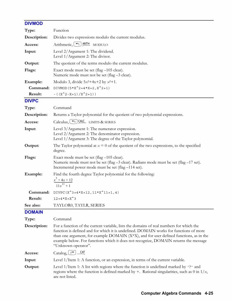
Computer Algebra Commands 4-25
DIVMOD Type: Function Description: Divides two expressions modulo the current modulus.
Access: Arithmetic, !Þ MODULO Input: Level 2/Argument 1: The dividend.
Level 1/Argument 2: The divisor. Output: The quotient of the terms modulo the current modulus. Flags: Exact mode must be set (flag 105 clear).
Numeric mode must not be set (flag 3 clear). Example: Modulo 3, divide 5x2+4x+2 by x2+1.
Command: DIVMOD(5*X^2+4*X+2,X^2+1)
Result: -((X^2-X+1)/X^2+1))
DIVPC Type: Command Description: Returns a Taylor polynomial for the quotient of two polynomial expressions.
Access: Calculus, !Ö LIMITS & SERIES Input: Level 3/Argument 1: The numerator expression.
Level 2/Argument 2: The denominator expression. Level 1/Argument 3: The degree of the Taylor polynomial.
Output: The Taylor polynomial at x = 0 of the quotient of the two expressions, to the specified degree.
Flags: Exact mode must be set (flag 105 clear). Numeric mode must not be set (flag 3 clear). Radians mode must be set (flag 17 set). Incremental power mode must be set (flag 114 set).
Example: Find the fourth degree Taylor polynomial for the following: x3 4x 12+ +
11x11 1+-----------------------------
Command: DIVPC(X^3+4*X+12,11*X^11+1,4)
Result: 12+4*X+X^3
See also: TAYLOR0, TAYLR, SERIES
DOMAIN Type: Command Description: For a function of the current variable, lists the domains of real numbers for which the
function is defined and for which it is undefined. DOMAIN works for functions of more than one argument, for example DOMAIN (X*X), and for user defined functions, as in the example below. For functions which it does not recognize, DOMAIN returns the message Unknown operator.
Access: Catalog, µ Input: Level 1/Item 1: A function, or an expression, in terms of the current variable. Output: Level 1/Item 1: A list with regions where the function is undefined marked by '?' and
regions where the function is defined marked by +. Rational singularities, such as 0 in 1/x, are not listed.
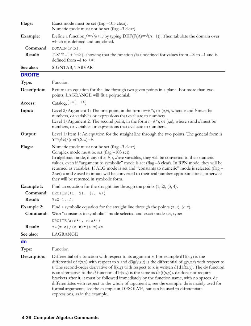
4-26 Computer Algebra Commands
Flags: Exact mode must be set (flag 105 clear). Numeric mode must not be set (flag 3 clear).
Example: Define a function f =√(a+1) by typing DEF(F(A)=√(A+1)). Then tabulate the domain over which it is defined and undefined.
Command: DOMAIN(F(X))
Result: '-∞' '?' 1 + '+∞', showing that the function f is undefined for values from ∞ to 1 and is defined from 1 to +∞.
See also: SIGNTAB, TABVAR
DROITE Type: Function Description: Returns an equation for the line through two given points in a plane. For more than two
points, LAGRANGE will fit a polynomial.
Access: Catalog, µ Input: Level 2/Argument 1: The first point, in the form a+b *i, or (a,b), where a and b must be
numbers, or variables or expressions that evaluate to numbers. Level 1/Argument 2: The second point, in the form c+d *i, or (c,d), where c and d must be numbers, or variables or expressions that evaluate to numbers.
Output: Level 1/Item 1: An equation for the straight line through the two points. The general form is Y=(d-b)/(c-a)*(X-a)+b.
Flags: Numeric mode must not be set (flag 3 clear). Complex mode must be set (flag 103 set). In algebraic mode, if any of a, b, c, d are variables, they will be converted to their numeric values, even if argument to symbolic mode is set (flag 3 clear). In RPN mode, they will be returned as variables. If ALG mode is set and constants to numeric mode is selected (flag 2 set) π and e used in inputs will be converted to their real number approximations, otherwise they will be returned in symbolic form.
Example 1: Find an equation for the straight line through the points (1, 2), (3, 4). Command: DROITE((1, 2), (3, 4))
Result: Y=X-1.+2.
Example 2: Find a symbolic equation for the straight line through the points (π, e), (e, π). Command: With constants to symbolic mode selected and exact mode set, type: DROITE(π+e*i, e+π*i) Result: Y=(π-e)/(e-π)*(X-π)+e
See also: LAGRANGE
dn Type: Function Description: Differential of a function with respect to its argument n. For example d1f(x,y) is the
differential of f(x,y) with respect to x and d3g(y,z,t) is the differential of g(y,z,t) with respect to t. The second-order derivative of f(x,y) with respect to x is written d1d1f(x,y). The dn function is an alternative to the ∂ function; d1f(x,y) is the same as ∂x(f(x,y)). dn does not require brackets after it, it must be followed immediately by the function name, with no spaces. dn differentiates with respect to the whole of argument n, see the example. dn is mainly used for formal arguments, see the example in DESOLVE, but can be used to differentiate expressions, as in the example.
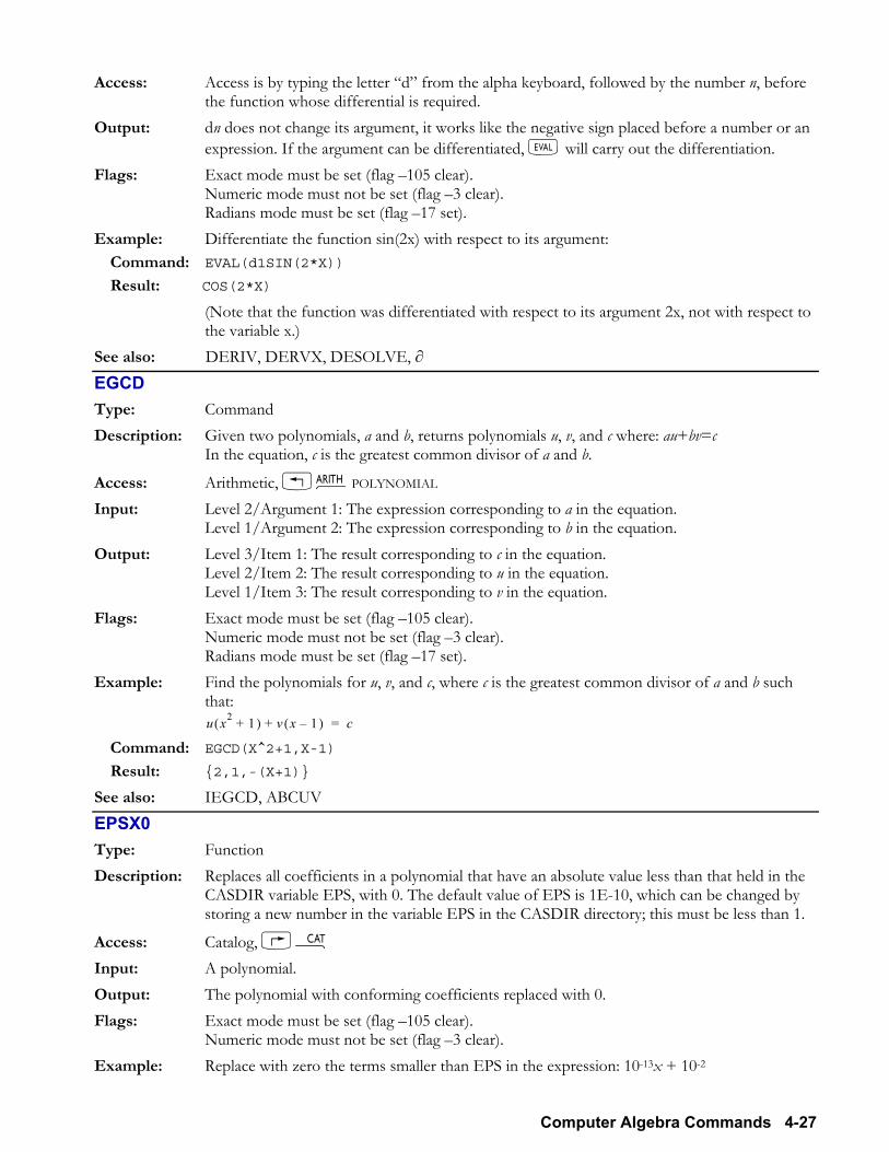
Computer Algebra Commands 4-27
Access: Access is by typing the letter d from the alpha keyboard, followed by the number n, before the function whose differential is required.
Output: dn does not change its argument, it works like the negative sign placed before a number or an expression. If the argument can be differentiated, N will carry out the differentiation.
Flags: Exact mode must be set (flag 105 clear). Numeric mode must not be set (flag 3 clear). Radians mode must be set (flag 17 set).
Example: Differentiate the function sin(2x) with respect to its argument: Command: EVAL(d1SIN(2*X))
Result: COS(2*X) (Note that the function was differentiated with respect to its argument 2x, not with respect to
the variable x.) See also: DERIV, DERVX, DESOLVE, ∂
EGCD Type: Command Description: Given two polynomials, a and b, returns polynomials u, v, and c where: au+bv=c
In the equation, c is the greatest common divisor of a and b.
Access: Arithmetic, !ÞPOLYNOMIAL Input: Level 2/Argument 1: The expression corresponding to a in the equation.
Level 1/Argument 2: The expression corresponding to b in the equation. Output: Level 3/Item 1: The result corresponding to c in the equation.
Level 2/Item 2: The result corresponding to u in the equation. Level 1/Item 3: The result corresponding to v in the equation.
Flags: Exact mode must be set (flag 105 clear). Numeric mode must not be set (flag 3 clear). Radians mode must be set (flag 17 set).
Example: Find the polynomials for u, v, and c, where c is the greatest common divisor of a and b such that: u x2 1+( ) v x 1( )+ c=
Command: EGCD(X^2+1,X-1)
Result: 2,1,-(X+1)
See also: IEGCD, ABCUV
EPSX0 Type: Function Description: Replaces all coefficients in a polynomial that have an absolute value less than that held in the
CASDIR variable EPS, with 0. The default value of EPS is 1E-10, which can be changed by storing a new number in the variable EPS in the CASDIR directory; this must be less than 1.
Access: Catalog, µ Input: A polynomial. Output: The polynomial with conforming coefficients replaced with 0. Flags: Exact mode must be set (flag 105 clear).
Numeric mode must not be set (flag 3 clear). Example: Replace with zero the terms smaller than EPS in the expression: 10-13x + 10-2
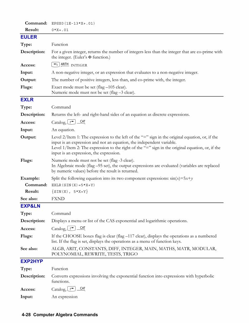
4-28 Computer Algebra Commands
Command: EPSX0(1E-13*X+.01)
Result: 0*X+.01
EULER Type: Function Description: For a given integer, returns the number of integers less than the integer that are co-prime with
the integer. (Eulers Φ function.)
Access: !ÞINTEGER Input: A non-negative integer, or an expression that evaluates to a non-negative integer. Output: The number of positive integers, less than, and co-prime with, the integer. Flags: Exact mode must be set (flag 105 clear).
Numeric mode must not be set (flag 3 clear).
EXLR Type: Command Description: Returns the left- and right-hand sides of an equation as discrete expressions.
Access: Catalog, µ Input: An equation. Output: Level 2/Item 1: The expression to the left of the = sign in the original equation, or, if the
input is an expression and not an equation, the independent variable. Level 1/Item 2: The expression to the right of the = sign in the original equation, or, if the input is an expression, the expression.
Flags: Numeric mode must not be set (flag -3 clear). In Algebraic mode (flag 95 set), the output expressions are evaluated (variables are replaced by numeric values) before the result is returned.
Example: Split the following equation into its two component expressions: sin(x)=5x+y Command: EXLR(SIN(X)=5*X+Y)
Result: SIN(X), 5*X+Y
See also: FXND
EXP&LN Type: Command Description: Displays a menu or list of the CAS exponential and logarithmic operations.
Access: Catalog, µ Flags: If the CHOOSE boxes flag is clear (flag 117 clear), displays the operations as a numbered
list. If the flag is set, displays the operations as a menu of function keys. See also: ALGB, ARIT, CONSTANTS, DIFF, INTEGER, MAIN, MATHS, MATR, MODULAR,
POLYNOMIAL, REWRITE, TESTS, TRIGO
EXP2HYP Type: Function
Description: Converts expressions involving the exponential function into expressions with hyperbolic functions.
Access: Catalog, µ Input: An expression
Computer Algebra Commands 4-29
Output: The rewritten expression. Flags: Exact mode must be set (flag 105 clear).
Numeric mode must not be set (flag -3 clear).
Example: Rewrite in terms of hyperbolic functions the expression e5 x( )ln⋅
Command: EXP2HYP(EXP(5*LN(X)))
Result: SINH(5*LN(X))+COSH(5*LN(X))
EXP2POW Type: Function
Description: Simplifies expressions involving the composition of the exponential and logarithmic functions. Compare this to LNCOLLECT which combines logarithmic terms; the difference is shown in the results of the second example used here and for LNCOLLECT.
Access: !Ú REWRITE Input: An expression
Output: The simplified expression. Flags: Exact mode must be set (flag 105 clear).
Numeric mode must not be set (flag -3 clear).
Example 1: Simplify the expression e 5·ln(x) Command: EXP2POW(EXP(5*LN(X)))
Result: X5
Example 2: Simplify the expression e n·ln(x) Command: EXP2POW(EXP(N*LN(X)))
Result: XN
See also: LNCOLLECT
EXPAND Type: Command Description: Expands and simplifies an algebraic expression. This command is similar to the EXPAN
command (which is included to ensure backward-compatibility with the HP 48-series calculators), except that EXPAND does more a more in-depth analysis and often does a better job at simplifying an expression than EXPAN.
Access: Algebra, ×or PALG
Input: An expression, or an array of expressions. Output: The expanded and simplified expression or array of expressions. Flags: Exact mode must be set (flag 105 clear).
Numeric mode must not be set (flag -3 clear). Radians mode must be set (flag 17 set).
Example: Simplify the following expression: x2 2x 1+ +( )
x 1+-------------------------------
Command: EXPAND((X^2+2*X+1)/(X+1))
Result: X+1
See also: EXPAN
4-30 Computer Algebra Commands
EXPANDMOD Type: Function Description: Expands and simplifies an algebraic expression, or an array of expressions, modulo the
current modulus.
Access: !ÞMODULO Input: An expression, or an array of expressions. Output: The expanded and simplified expression, or array of expressions, modulo the current
modulus. Flags: Exact mode must be set (flag 105 clear).
Numeric mode must not be set (flag -3 clear). Radians mode must be set (flag 17 set).
Example: Expand the following expression and give the result modulo 3: x 3+( ) x 4+( )
Command: EXPANDMOD((X+3)*(X+4))
Result: X^2+X
EXPLN Type: Command Description: Transforms the trigonometric terms in an expression to exponential and logarithmic terms.
Access: !Ð or Convert, !Ú REWRITE or PLEXP & LN
Input: An expression Output: The transformed expression. Flags: Exact mode must be set (flag 105 clear).
Numeric mode must not be set (flag -3 clear). Radians mode must be set (flag 17 set). Complex mode must be set (flag 103 set).
Example: Transform the following expression and simplify the result using the EXPAND command: 2 x2( )cos
Command: EXPLN(2*COS(X^2))
EXPAND(ANS(1))
Result: (EXP(i*X^2)^2+1)/EXP(i*X^2) See also: SINCOS
FACTOR Type: Command Description: Factorizes a polynomial or an integer:
The function expresses a polynomial as the product of irreducible polynomials. The function expresses an integer as the product of prime numbers.
Access: Algebra, ×or PALG or !ÞPOLY
Input: An expression or an integer. Output: The factorized expression, or the integer expressed as the product of prime numbers. Flags: Exact mode must be set (flag 105 clear).
Numeric mode must not be set (flag -3 clear). Results including complex terms are returned if complex mode is set (flag 103 set).
Computer Algebra Commands 4-31
Example: Factorize the following: x2 5x 6+ +
Command: FACTOR(X^2+5*X+6)
Result: (X+2)(X+3)
See also: EXPAN, EXPAND
FACTORMOD Type: Function Description: Factorizes a polynomial modulo the current modulus. The modulus must be less than 100,
and a prime number, it can be changed by MODSTO.
Access: Arithmetic, !Þ MODULO Input: The expression to be factorized. Output: The factorized expression modulo the current modulus. Flags: Exact mode must be set (flag 105 clear).
Numeric mode must not be set (flag -3 clear). Radians mode must be set (flag 17 set).
Example: Factorize the following expression modulo 3. x2+2
Command: FACTORMOD(X^2+2)
Result: (X+1)*(X-1)
See also: MODSTO
FACTORS Type: Command Description: For a value or expression, returns a list of prime factors and their multiplicities.
Access: Arithmetic, !Þ
Input: A value or expression. Output: A list of prime factors of the value or expression, with each factor followed by its multiplicity
expressed as a real number. Flags: Exact mode must be set (flag 105 clear).
Numeric mode must not be set (flag -3 clear). Radians mode must be set (flag 17 set).
Example 1: Find the prime factors of 100. Command: FACTORS(100)
Result: 5 2. 2 2.
Example 2: Find the irreducible factors of: x2 4x 4+ + Command: FACTORS(X^2+4*X+4)
Result: X+2,2.
FCOEF Type: Command Description: From an array of roots and multiplicities/poles, returns a rational polynomial with a leading
coefficient of 1, with the specified set of roots or poles, and with the specified multiplicities.
Access: Arithmetic, !ÞPOLY L
4-32 Computer Algebra Commands
Input: An array of the form [Root 1, multiplicity/pole 1, Root 2, multiplicity/pole 2, . . .] The multiplicity/pole must be an integer. A positive number signifies a multiplicity. A negative number signifies a pole.
Output: The rational polynomial with the specified roots and multiplicities/poles. The polynomial is written using the current independent variable.
Flags: Exact mode must be set (flag 105 clear). Numeric mode must not be set (flag -3 clear).
Example: Find the rational polynomial corresponding to the following set of roots and poles: 1, 2, 3, 1
Command: FCOEF([1,2,3,-1])
Result: (X-1)^2/(X-3)
See also: FROOTS
FDISTRIB Type: Command
Description: Performs a full distribution of multiplication and division with respect to addition and subtraction in a single step.
Access: !Ú REWRITE Input: An expression. Output: An equivalent expression that results from fully applying the distributive property of
multiplication and division over addition and subtraction. Flags: Exact mode must be set (flag 105 clear).
Numeric mode must not be set (flag -3 clear). Example: Expand (X+1)(X-1)(X+2):
Command: FDISTRIB((X+1)*(X-1)*(X+2))
Result: X*(X*X)+2*(X*X)+(-(X*(1*X))+-(2*(1*X)))+ (X*(X*1)+2*(X*1)+
(-(X*(1*1))+-(2*(1*1))))
See also: DISTRIB
FOURIER Type: Function Description: Returns the nth coefficient of a complex Fourier series expansion. The PERIOD variable must
be in the CAS directory, CASDIR, or in current path, and set to hold L, the period of the input function. The expression is expanded in terms of the current CAS variable.
Access: Calculus !ÖDERIV. & INTEG. Input: Level 1/Argument 2: An expression in terms of the current variable
Level 2/Argument 1: The number, n, of the coefficient to return. Output: The nth Fourier coefficient of the expression. Flags: Exact mode must be set (flag 105 clear).
Numeric mode must not be set (flag -3 clear). Radians mode must be set (flag 17 set). Complex mode must be set, that is, flag 103 must be set.
Example: Obtain the Fourier coefficient as below, with the default value of 2π in the PERIOD variable in CASDIR, and simplify it with EXPAND:
Computer Algebra Commands 4-33
Command: FOURIER(X^2,0)
EXPAND(ANS(1))
Result: 4/3* π^2
FROOTS Type: Command Description: For a rational polynomial, returns an array of its roots and poles, with their corresponding
multiplicities. This is the inverse of FCOEF and uses the same notation for roots and poles.
Access: Arithmetic, !ÞPOLY L Input: A rational polynomial. Output: An array of the form [Root 1, Multiplicity 1, Root 2, Multiplicity 2, . . .]
A negative multiplicity indicates a pole. Flags: Exact mode must be set (flag 105 clear). Numeric mode must not be set (flag -3 clear).
Radians mode must be set (flag 17 set). If complex mode is set (flag 103 set), FROOTS looks for complex solutions as well as real solutions. If approximate mode is set (flag 105 set) FROOTS searches for numeric roots.
See also: FCOEF
FXND Type: Command Description: Splits an object into a numerator and a denominator.
Access: Catalog, µ Input: A fraction, or an object that evaluates to a fraction. Output: The object split into numerator and denominator.
Level 2/Item 1: The numerator. Level 1/Item 2: The denominator.
Flags: Exact mode must be set (flag 105 clear). Numeric mode must not be set (flag -3 clear).
Example: Return the numerator and the denominator of the following expression: x 3( )2
z 4+-------------------
Command: FXND((X-3)^2/(Z+4))
Result: (X-3)^2, Z+4
See also: EXLR
GAUSS Type: Command Description: Returns the diagonal representation of a quadratic form.
Access: Matrices, !Ø QUADRATIC FORM Input: Level 2/Argument 1: The quadratic form.
Level 1/Argument 2: A vector containing the independent variables. Output: Level 4/Item 1: An array of the coefficients of the diagonal.
Level 3/Item 2: A matrix, P, such that the quadratic form is represented as PTDP, where the diagonal matrix D contains the coefficients of the diagonal representation.

4-34 Computer Algebra Commands
Level 2/Item 3: The diagonal representation of the quadratic form. Level 1/Item 4: The vector of the variables.
Flags: Exact mode must be set (flag 105 clear). Numeric mode must not be set (flag -3 clear). Radians mode must be set (flag 17 set).
Example: Find the Gaussian symbolic quadratic form of the following: x2 2axy+
Command: GAUSS(X^2+2*A*X*Y,[X,Y])
Result: [1,-A^2], [[1,A][0,1]], -(A^2*Y^2)+(A*Y+X)^2,[X,Y]
See also: AXQ, QXA
GBASIS Type: Command Description: Returns a set of polynomials that are a Grbner basis G of the ideal I generated from an
input set of polynomials F.
Access: Catalog, µ Input: Level 2/Argument 1: A vector F of polynomials in several variables.
Level 1/Argument 2: A vector giving the names of the variables. Output: Level 1/Item 1: A vector containing the resulting set G of polynomials. The command
attempts to order the polynomials as given in the vector of variable names. Flags: Exact mode must be set (flag 105 clear).
Numeric mode must not be set (flag -3 clear). Radians mode must be set (flag 17 set).
Example: Find a Grbner basis of the ideal polynomial generated by the polynomials: x2 + 2xy2, xy + 2y3 1
Command: GBASIS([X^2 + 2*X*Y^2, X*Y + 2*Y^3 – 1], [X,Y])
Result: [X, 2*Y^3-1] Note this is not the minimal Grbner basis, as the leading coefficient of the second term is not 1; the algorithm used avoids giving results with fractions.
See also: GREDUCE
GCD Type: Function Description: Returns the greatest common divisor of two objects.
Access: Arithmetic, !ÞPOLY L Input: Level 2/Argument 1: An expression, or an object that evaluates to a number.
Level 1/Argument 2: An expression, or an object that evaluates to a number. Output: The greatest common divisor of the two objects. Flags: Exact mode must be set (flag 105 clear).
Numeric mode must not be set (flag -3 clear). Example: Find the greatest common divisor of 2805 and 99.
Command: GCD(2805,99)
Result: 33
See also: GCDMOD, EGCD, IEGCD, LCM
Computer Algebra Commands 4-35
GCDMOD Type: Function Description: Finds the greatest common divisor of two polynomials modulo the current modulus.
Access: Arithmetic, !ÞMODULO Input: Level 2/Argument 1: A polynomial expression.
Level 1/Argument 2: A polynomial expression. Output: The greatest common divisor of the two expressions modulo the current modulus. Flags: Exact mode must be set (flag 105 clear).
Numeric mode must not be set (flag -3 clear). Radians mode must be set (flag 17 set).
Example: Find the greatest common divisor of 2x^2+5 and 4x^2-5x, modulo 13. Command: GCDMOD(2X^2+5,4X^2-5X)
Result: -(4X-5)
See also: GCD
GRAMSCHMIDT Type: Command
Description: Finds an orthonormal base of a vector space with respect to a given scalar product.
Access: Matrices, !Ø LVECTOR
Input: Level 2/Argument 1: A vector representing a basis of a vector space. Level 1/Argument 2: A function that defines a scalar product in that space. This can be given as a program, or as the name of a variable containing the definition of the function.
Output: An orthonormal base of the vector space with respect to the given scalar product. Flags: Exact mode must be set (flag 105 clear).
Numeric mode must not be set (flag -3 clear). Radians mode must be set (flag 17 set).
Example: Find an orthonormal base for the vector space with base [1, 1+X] with respect to the scalar product defined by :
P Q⋅ P x( ) Q x( )⋅ xd1
1∫=
Command: GRAMSCHMIDT([1,1+X], « → P Q « PREVAL(INTVX(P*Q),-1,1) » »)
Result:
12
------- X13--- 6⋅--------------
GREDUCE Type: Command Description: Reduces a polynomial with respect to a Grbner basis.
Access: Catalog, µ Input: Level 3/Argument 1: A vector of polynomials in several variables.
Level 2/Argument 2: A vector of polynomials that is a Grbner basis in the same variables. Level 1/Argument 3: A vector giving the names of the variables.
Output: Level 1/Item 1: A vector containing the input polynomial reduced with respect to the Grbner basis, up to a constant; as with GBASIS, fractions in the result are avoided.
4-36 Computer Algebra Commands
Flags: Exact mode must be set (flag 105 clear). Numeric mode must not be set (flag -3 clear). Radians mode must be set (flag 17 set).
Example: Reduce the polynomial: x2y xy 1 with respect to the Grbner basis (obtained in the example for GBASIS): x, 2y3 1
Command: GREDUCE(X^2*Y–X*Y–1, [X,2*Y^3–1], [X,Y])
Result: -1 Note this is the remainder of the input polynomial modulo the term x in the Grbner basis
See also: GBASIS
HADAMARD Type: Command Description: Performs an element by element multiplication of two matrices (Hadamard product).
Access: Matrices, !Ø OPERATIONS L Input: Level 2/Argument 1: Matrix 1.
Level 1/Argument 2: Matrix 2. The matrices must have the same order.
Output: The matrix representing the result of the multiplication. Flags: Exact mode must be set (flag 105 clear).
Numeric mode must not be set (flag -3 clear). Example: Find the Hadamard product of the following two matrices:
3 1 20 1 4 and
2 3 01 5 2
Command: HADAMARD([[3,-1,2][0,1,4]],[2,3,0][1,5,2]])
Result: [[6,-3,0][0,5,8]]
HALFTAN Type: Command Description: Transforms an expression by replacing sin(x), cos(x) and tan(x) subexpressions with tan(x/2)
terms.
Access: Trigonometry, Ñor P TRIG
Input: An expression Output: The transformed expression. Flags: Exact mode must be set (flag 105 clear).
Numeric mode must not be set (flag -3 clear). Radians mode must be set (flag 17 set).
See also: TAN2CS2, TAN2SC2
HELP Type: Command Description: Similar to CASCMD, displays a list of CAS operations. Selecting one with OK displays help
for it, an example of the operation, and the option to copy the example to the command line. More details are given in Appendix C and Appendix H of the Users Guide.
Computer Algebra Commands 4-37
Access: Catalog, µ, or tools IL See also: CASCMD
HERMITE Type: Function Description: Returns the nth Hermite polynomial.
Access: Arithmetic, !ÞPOLY L Input: A non-negative integer. Output: The corresponding polynomial expression. Flags: Exact mode must be set (flag 105 clear).
Numeric mode must not be set (flag -3 clear). Example: Find the Hermite polynomial with degree 4.
Command: HERMITE(4)
Result: 16*X^4-48*X^2+12 See also: LEGENDRE, TCHEBYCHEFF
HESS Type: Command Description: Returns the Hessian matrix and the gradient of an expression with respect to the specified
variables.
Access: Calculus !ÖDERIV & INTEG Input: Level 2/Argument 1: An expression.
Level 1/Argument 2: A vector of the variables. Output: Level 3/Item 1: The Hessian matrix with respect to the specified variables.
Level 2/Item 2: The gradient with respect to the variables. Level 1/Item 3: The vector of the variables.
Flags: Exact mode must be set (flag 105 clear). Numeric mode must not be set (flag -3 clear).
Example: Find the Hessian matrix, and the gradient with respect to each variable, of the expression: t2 + 2tu2.
Command: HESS(T^2+2*T*U^2, [T, U])
Result: [[2, 2*(2*U)], [2*(2*U), 2*(2*T)]], [2*T+2*U^2, 2*T*(2*U)], [T, U]
See also: CURL, DIV
HILBERT Type: Command Description: Returns a square Hilbert matrix of the specified order.
Access: Matrices, !Ø CREATE Lor !´ MATRX MAKE LL Input: A positive integer, representing the order. Output: The Hilbert matrix of the specified order. Flags: Exact mode must be set (flag 105 clear).
Numeric mode must not be set (flag -3 clear). Example: Find the order 3 Hilbert matrix.
Command: HILBERT(3)
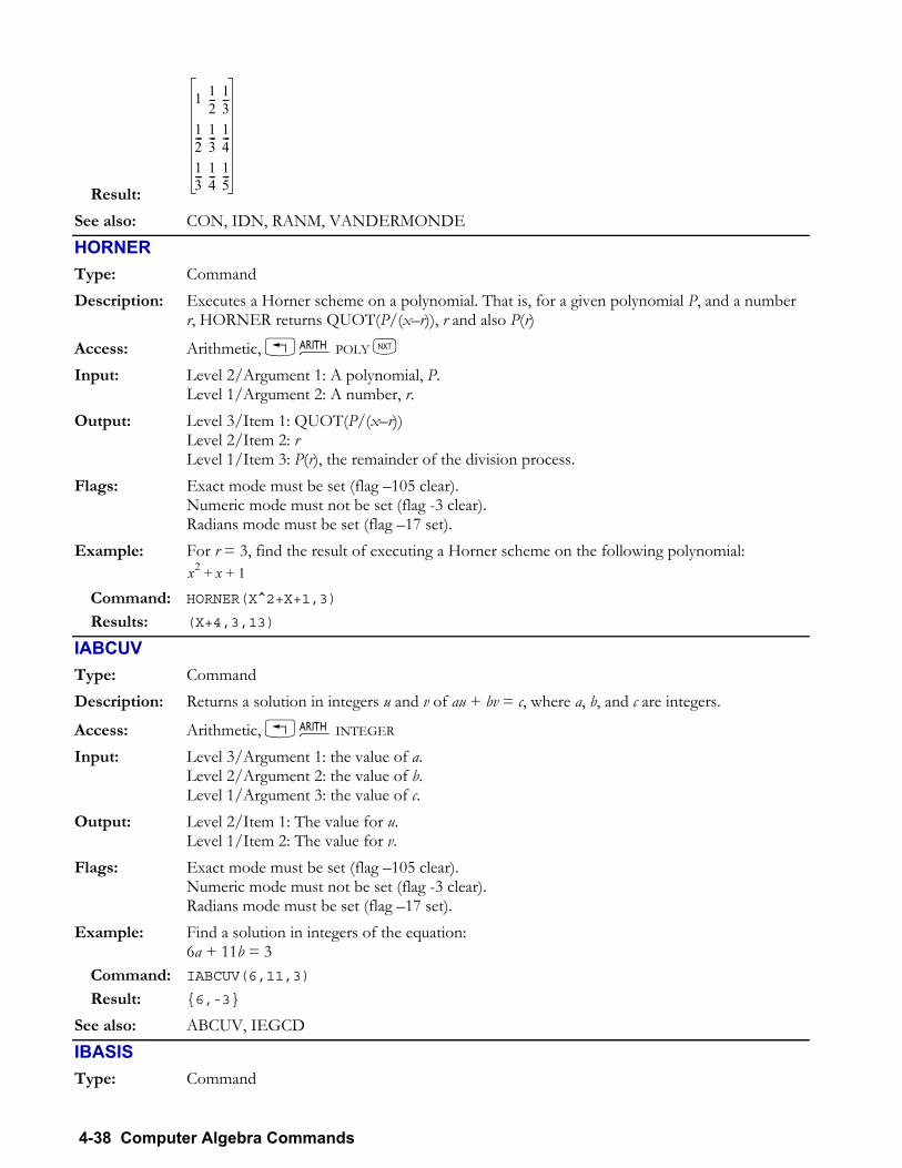
4-38 Computer Algebra Commands
Result:
1 12--- 1
3---
12--- 1
3--- 1
4---
13---
14---
15---
See also: CON, IDN, RANM, VANDERMONDE
HORNER Type: Command Description: Executes a Horner scheme on a polynomial. That is, for a given polynomial P, and a number
r, HORNER returns QUOT(P/(xr)), r and also P(r)
Access: Arithmetic, !ÞPOLY L Input: Level 2/Argument 1: A polynomial, P.
Level 1/Argument 2: A number, r. Output: Level 3/Item 1: QUOT(P/(xr))
Level 2/Item 2: r Level 1/Item 3: P(r), the remainder of the division process.
Flags: Exact mode must be set (flag 105 clear). Numeric mode must not be set (flag -3 clear). Radians mode must be set (flag 17 set).
Example: For r = 3, find the result of executing a Horner scheme on the following polynomial: x2 x 1+ +
Command: HORNER(X^2+X+1,3)
Results: (X+4,3,13)
IABCUV Type: Command Description: Returns a solution in integers u and v of au + bv = c, where a, b, and c are integers.
Access: Arithmetic, !ÞINTEGER Input: Level 3/Argument 1: the value of a.
Level 2/Argument 2: the value of b. Level 1/Argument 3: the value of c.
Output: Level 2/Item 1: The value for u. Level 1/Item 2: The value for v.
Flags: Exact mode must be set (flag 105 clear). Numeric mode must not be set (flag -3 clear). Radians mode must be set (flag 17 set).
Example: Find a solution in integers of the equation: 6a + 11b = 3
Command: IABCUV(6,11,3)
Result: 6,-3
See also: ABCUV, IEGCD
IBASIS Type: Command
Computer Algebra Commands 4-39
Description: Determines the basis of the intersection between two vector spaces.
Access: Matrices, !Ø L VECTOR
Input: Two lists of vectors
Output: A list of vectors. Flags: Exact mode must be set (flag 105 clear). Example: Find a vector of a basis of the intersection of the vector sub-spaces defined by [1, 2] and [2, 4]
Command: IBASIS([1,2], [2,4])
Result: [1,2] See also: BASIS
IBERNOULLI Type: Function Description: Returns the nth Bernoulli number for a given integer n.
Access: Arithmetic, !ÞINTEGER Input: Level 1/Argument 1: an integer. Output: Level 1/Item 1: The corresponding nth Bernoulli number for the integer. For numbers greater
than about 40 the calculation can take a long time. Flags: Numeric mode must not be set (flag -3 clear).
IBP Type: Command Description: Performs integration by parts on a function. The function must be able to be represented as a
product of two functions, where the antiderivative of one of the functions is known: f(x) = u(x).v’(x)
Note that the command is designed for use in RPN mode only.
Access: PCALC or Calculus, !ÖDERIV & INTEG L Input: Level 2: The integrand expressed as a product of two functions, u(x).v’(x)
Level 1: The antiderivative of one of the component functions, v(x). Output: Level 2: u(x)v(x)
Level 1: -u'(x)v(x) Flags: Exact mode must be set (flag 105 clear).
Numeric mode must not be set (flag -3 clear). Radians mode must be set (flag 17 set).
Example: Use integration by parts to calculate the following: x x( )cos xd∫
Command 1: Apply the IBP command in RPN mode: Level 2: X*COS(X)
Level 1: SIN(X) Result: Level 2: SIN(X)*X
Level 1: -SIN(X) Command 2: Apply the INTVX command to level 1, -SIN(X) Result: Level 2: SIN(X)*X
Level 1: COS(X) Command 3: Press + to add the result to the value at level 2 to obtain the final result.
4-40 Computer Algebra Commands
x 2≡x 1≡
Result: SIN(X)*(X)+COS(X)
See also: INTVX, INT, PREVAL, RISCH
ICHINREM Type: Command Description: Solves a system of two congruences in integers using the Chinese Remainder theorem.
Access: Arithmetic, !ÞINTEGER Input: Level 2/Argument 1: A vector of the first value and the modulus.
Level 1/Argument 2: A vector of the second value and the modulus. Output: A vector of the solution. Flags: Exact mode must be set (flag 105 clear).
Numeric mode must not be set (flag -3 clear). Radians mode must be set (flag 17 set).
Example: Solve the following system of congruences: Modulo 3 Modulo 5
Command: ICHINREM([2,3],[1,5])
Results: [-4, 15] See also: CHINREM
IDIV2 Type: Command Description: For two integers, a and b, returns the integer part of a/b, and the remainder, r.
Access: Arithmetic, !ÞINTEGER Input: Level 2/Argument 1: a.
Level 1/Argument 2: b. Output: Level 2/Item 1: The integer part of a/b.
Level 1/Item 2: The remainder. Flags: Numeric mode must not be set (flag -3 clear).
Radians mode must be set (flag 17 set). Example: Return the integer part and the remainder of 11632/864.
Command: IDIV2(11632,864)
Result: 13,400 See also: DIV2, IQUOT
IEGCD Type: Command Description: Given two integers x and y, returns three integers, a, b, and c, such that:
ax+by=c where c is the GCD of x and y.
Access: PARITH or Arithmetic, !ÞINTEGER Input: Level 2/Argument 1: x.
Level 1/Argument 2: y. Output: Level 3/Item 1: c.
Level 2/Item 2: a.
Computer Algebra Commands 4-41
Level 1/Item 3: b. Note the order, c is first.
Flags: Exact mode must be set (flag 105 clear). Numeric mode must not be set (flag -3 clear). Radians mode must be set (flag 17 set).
Example: Find a, b and c such that a18 + b24 = c, where c is the GCD of 18 and 24. Command: IEGCD(18,24)
Result: 6,-1,1 See also: ABCUV, EGCD, IABCUV
ILAP Type: Function Description: Returns the inverse Laplace transform of an expression. The expression must evaluate to a
rational fraction.
Access: Calculus, !ÖDIFFERENTIAL EQNS Input: A rational expression. Output: The inverse Laplace transformation of the expression. Flags: Exact mode must be set (flag 105 clear).
Numeric mode must not be set (flag -3 clear). Radians mode must be set (flag 17 set).
Example: Find the inverse Laplace transform of:
Command: ILAP(1/(X-5)^2)
Result: X*EXP(5*X) See also: LAP, LAPL
IMAGE Type: Command
Description: Computes the basis of the image (also called the range) of a linear application f.
Access: Matrices, !Ø LINEAR APPL
Input: A matrix representing a linear application f in terms of the standard basis. Output: A list of vectors representing a basis of the image of f. Flags: Exact mode must be set (flag 105 clear).
Numeric mode must not be set (flag -3 clear).
Example: Find the image of
1 1 22 1 33 1 4
Command: IMAGE([1,1,2] [2,1,3] [3,1,4]) Result: [1,0,-1] [0,1,2]
See also: BASIS, KER
INT Type: Function Description: Calculates the antiderivative of a function for a given variable, at a given point.
Access: Catalog, µ
1x 5( )2-------------------
4-42 Computer Algebra Commands
Input: Level 3/Argument 1: A function. Level 2/Argument 2: The variable to obtain the derivative with respect to. Level 1/Argument 3: The point at which to calculate the antiderivative. This point can be a variable or an expression.
Output: The antiderivative of the function for the given variable, at the point you specified. Flags: Exact mode must be set (flag 105 clear).
Numeric mode must not be set (flag -3 clear). Radians mode must be set (flag 17 set).
Example: Find the integral of sin(x) with respect to x, at the point where x=y. Command: INT(SIN(X),X,Y) Result: -COS(Y)
See also: INTVX, RISCH
INTEGER Type: Command Description: Displays a menu or list of CAS integer operations.
Access: Catalog, µ Flags: If the CHOOSE boxes flag is clear (flag 117 clear), displays the operations as a numbered
list. If the flag is set, displays the operations as a menu of function keys. See also: ALGB, ARIT, CONSTANTS, DIFF, EXP&LN, MAIN, MATHS, MATR, MODULAR,
POLYNOMIAL, REWRITE, TESTS, TRIGO
INTVX Type: Function Description: Finds the antiderivative of a function symbolically, with respect to the current default variable.
Access: Calculus, !Öor P CALC or !Ö DERIV. & INTEG L Input: An expression. Output: The antiderivative of the expression. Flags: Exact mode must be set (flag 105 clear).
Numeric mode must not be set (flag -3 clear). Radians mode must be set (flag 17 set).
Example: Find the antiderivative of the following: x2 xln
Command: INTVX(X^2*LN(X))
Result: 1/3*X^3*LN(X)+(-1/9)*X^3
See also: IBP, RISCH, PREVAL
INVMOD Type: Function Description: Performs modular inversion on an object modulo the current modulus.
Access: Arithmetic, !ÞMODULO L Input: An object. Output: The modular inverse of the object.
Computer Algebra Commands 4-43
Flags: Exact mode must be set (flag 105 clear). Numeric mode must not be set (flag -3 clear).
Example: Solve the following for x, modulo the default modulus, 13. 2x 1≡( )
Command: INVMOD(2)
Result: -6
IQUOT Type: Function Description: Returns the integer quotient (or Euclidean quotient) of two integers. That is, given two
integers, a and b, returns the integer q, such that: a = qb + r, and 0 ≤ r < b
Access: PARITH or Arithmetic, !ÞINTEGER L Input: Level 2/Argument 1: The dividend.
Level 1/Argument 2: The divisor. Output: The integer quotient. Flags: Exact mode must be set (flag 105 clear).
Numeric mode must not be set (flag -3 clear). Radians mode must be set (flag 17 set).
See also: QUOT, IDIV2
IREMAINDER Type: Function Description: Returns the remainder of an integer division.
Access: PARITH or Arithmetic, !ÞINTEGER L Input: Level 2/Argument 1: The numerator.
Level 1/Argument 2: The denominator. Output: The remainder. Flags: Exact mode must be set (flag 105 clear).
Numeric mode must not be set (flag -3 clear). Radians mode must be set (flag 17 set).
See also: IDIV2
ISOM Type: Command
Description: Determine the characteristics of a 2-d or 3-d linear isometry.
Access: Matrices, !Ø LINEAR APPL
Input: A square matrix representing a linear isometry. Output: A vector and/or an angle that represent the symmetry of the matrix, and 1 (for a direct
isometry) or -1 (for an indirect isometry). Flags: Exact mode must be set (flag 105 clear).
Numeric mode must not be set (flag -3 clear). Radians mode must be set (flag 17 set).
4-44 Computer Algebra Commands
Example 1: Analyze the isometry given by the matrix 0 11 0
Command: ISOM([[0,-1] [-1,0]])
Result: [1, 1] 1, meaning the matrix represents a symmetry in the line y = x, and this is an indirect isometry.
Example 2: Analyze the isometry given by the matrix
12---
32----------
32
------- 12---
Command: ISOM([[1/2, -√3/2][√3/2, 1/2]])
Result: π/3, 1 , meaning the matrix represents a rotation of π/3 radians, and this is a direct isometry. See also: MKISOM
ISPRIME? Type: Function Description: Tests if a number is prime. For numbers of the order of 1014 or greater (to be exact, greater
than 341550071728321), tests if the number is a pseudoprime; this has a chance of less than 1 in 1012 of wrongly identifying a number as a prime.
Access: PARITH or Arithmetic, !ÞINTEGER L Input: An object that evaluates to an integer or a whole real number. Output: 1 (True) if the number is prime, 0 (False) if it is not. Flags: Exact mode must be set (flag 105 clear).
Numeric mode must not be set (flag -3 clear). See also: NEXTPRIME, PREVPRIME
JORDAN Type: Command Description: Diagonalization, or Jordan cycle decomposition, of a matrix. Computes the eigenvalues,
eigenvectors, minimum polynomial, and characteristic polynomial of a matrix.
Access: Matrices, !Ø LEIGENVECTORS Input: An n × n matrix. Output: Level 4/Item 1: The minimum polynomial.
Level 3/Item 2: The characteristic polynomial. Level 2/Item 3: A list of characteristic spaces tagged by the corresponding eigenvalue (either a vector or a list of Jordan chains, each of them ending with an "Eigen:"-tagged eigenvector). Level 1/Item 4: An array of the eigenvalues, with multiplicities
Flags: Exact mode must be set (flag 105 clear). Numeric mode must not be set (flag -3 clear). Radians mode must be set (flag 17 set).
Example: Perform the following diagonalization: Command: JORDAN([1,1][1,1]) Result: X^2-2*X,
X^2-2*X,
Computer Algebra Commands 4-45
0: [1,-1], 2: [1,1] [0,2]
KER Type: Command
Description: Computes the basis of the kernel of a linear application f.
Access: Matrices, !Ø LINEAR APPL
Input: A matrix representing a linear application f in terms of the standard basis. Output: A list of vectors representing a basis of the kernel (also called the nullspace) of f. Flags: Exact mode must be set (flag 105 clear).
Numeric mode must not be set (flag -3 clear).
Example: Find the kernel of
1 1 22 1 33 1 4
Command: KER([1,1,2][2,1,3][3,1,4]) Result: [1,1,-1]
See also: BASIS, IMAGE
LAGRANGE Type: Command Description: Returns the interpolating polynomial of minimum degree for a set of pairs of values. For two
pairs, DROITE will fit a straight line.
Access: Arithmetic, !ÞPOLY L Input: A two × n matrix of the n pairs of values. Output: The polynomial that results from the Lagrange interpolation of the data. Flags: Exact mode must be set (flag 105 clear).
Numeric mode must not be set (flag -3 clear). Radians mode must be set (flag 17 set).
Example: Find an interpolating polynomial for the data (1,6), (3,7), (4,8), (2,9) Command: LAGRANGE([[1,3,4,2][6,7,8,9]])
Result: 8x3 63x2 151x 60+
6--------------------------------------------------------
See also: DROITE
LAP Type: Function Description: Performs a Laplace transform on an expression with respect to the current default variable.
Access: Calculus, !Ö DIFFERENTIAL EQNS Input: An expression. Output: The Laplace transform of the expression. Flags: Exact mode must be set (flag 105 clear).
Numeric mode must not be set (flag -3 clear). Radians mode must be set (flag 17 set).
4-46 Computer Algebra Commands
Example: Find the Laplace transform of ex. Command: LAP(EXP(X))
Result: 1/(X-1)
See also: ILAP, LAPL
LAPL Type: Command Description: Returns the Laplacian of a function with respect to a list of variables.
Access: !Ö DERIV & INTEG L Input: Level 2/Argument 1:An expression.
Level 1/Argument 2: A vector of variables. Output: The Laplacian of the expression with respect to the variables. Flags: Exact mode must be set (flag 105 clear).
Numeric mode must not be set (flag -3 clear). Radians mode must be set (flag 17 set).
Example: Find, and simplify, the Laplacian of the following expression: ex zy( )cos
Command: LAPL(EXP(X)*COS(Z*Y),[X,Y,Z])
EXPAND(ANS(1))
Result: -((Y^2+Z^2-1)*EXP(X)*COS(Z*Y))
See also: LAP, ILAP
LCM Type: Function Description: Returns the least common multiple of two objects.
Access: Arithmetic, !ÞPOLYNOMIAL LL Input: Level 2/Argument 1: An expression, a number, or object that evaluates to a number.
Level 1/Argument 2: An expression, a number, or object that evaluates to a number. Output: The least common multiple of the objects. Flags: Exact mode must be set (flag 105 clear).
Numeric mode must not be set (flag -3 clear). Radians mode must be set (flag 17 set).
Example: Find the least common multiple of the following two expressions: x2 1 x1
Command: LCM(X^2-1,X-1)
Results: X^2-1
See also: GCD
LCXM Type: Command Description: From a program with two arguments, builds a matrix with the specified number of rows and
columns, with aij = f(i,j).
Access: Catalog, µ
Computer Algebra Commands 4-47
Input: Level 3/Argument 1: The number of rows you want in the resulting matrix. Level 2/Argument 2: The number of columns you want in the resulting matrix. Level 1/Argument 3: A program that uses two arguments. An expression with the two variables I, J can be used instead.
Output: The resulting matrix. Flags: Exact mode must be set (flag 105 clear).
Numeric mode must not be set (flag -3 clear). Example: Build a 2 × 3 matrix with aij=i+2j.
Command: LCXM(2,3,« →I J 'I+2*J'»)
Result:
3 5 74 6 8
LDEC Type: Command Description: Solves a linear differential equation with constant coefficients, or a system of first order linear
differential equations with constant coefficients.
Access: Symbolic solve, !Îor PSOLVER or !ÖDIFF
Input: Level 2/Argument 1: For a single equation, the function forming the right hand side of the equation. For a system of equations, an array comprising the terms not containing the dependent variables. Level 1/Argument 2: For one equation, the auxiliary polynomial. For a system of equations, the matrix of coefficients of the dependent variables.
Output: The solution. Flags: Exact mode must be set (flag 105 clear).
Numeric mode must not be set (flag -3 clear). Radians mode must be set (flag 17 set).
Example: Solve 2sin(x), with the auxiliary polynomial x2+1: Command: LDEC(2*SIN(X),X^2+1) Result: COS(X)*(cC0 -X)+(cC1 — -1)*SIN(X)
See also: DESOLVE
LEGENDRE Type: Function Description: Returns the nth degree Legendre polynomial.
Access: Arithmetic, !Þ POLYNOMIAL LL Input: An integer, n. Output: The nth Legendre polynomial. Flags: Exact mode must be set (flag 105 clear).
Numeric mode must not be set (flag -3 clear). Example: Find the Legendre polynomial with degree 4.
Command: LEGENDRE(4)
Result: (35*X^4-30*X^2+3)/8
See also: HERMITE, TCHEBYCHEFF
4-48 Computer Algebra Commands
LGCD Type: Function Description: Returns the greatest common divisor of a list of expressions or values.
Access: Arithmetic, !Þ L Input: A list of expressions or values. Output: Level 2/Item 1: The list of elements.
Level 1/Item 2: The greatest common divisor of the elements. Flags: Exact mode must be set (flag 105 clear).
Numeric mode must not be set (flag -3 clear). Radians mode must be set (flag 17 set).
See also: GCD
LIMIT Type: Function Description: Returns the limit of a function as its argument approaches a specified value. This function is
identical to the lim function, described below, and is included to ensure backward-compatibility with the HP49G calculator.
Access: Catalog, µ
lim Type: Function Description: Returns the limit of a function as its argument approaches a specified value. Expands and
simplifies an algebraic expression.
Access: Calculus, !Ö LIMITS&SERIES Input: Level 2/Argument 1: An expression. Level 1/Argument 2: An expression of the form x = y, where x is the variable and y is the
value at which the limit is to be evaluated. If the variable approaching a value is the current CAS variable, it is sufficient to give its value alone. The ∞ symbol provided by the calculator can be used to set the limiting value at plus or minus infinity.
Output: The limit of the expression at the limit point. Flags: Exact mode must be set (flag 105 clear).
Numeric mode must not be set (flag -3 clear). Radians mode must be set (flag 17 set).
Example: Find the following limit: lim
x y→⎝ ⎠⎛ ⎞ xn yn
x y----------------
Command: lim((X^N-Y^N)/(X-Y), X=Y)
Result: N*EXP(N*LN(Y))/Y
See also: SERIES
LIN Type: Command Description: Linearizes expressions involving exponential terms.
Access: × or Exponential and logarithm, !Ð or PALG, or !Ú REWRITE, or PLEXPLN.
Computer Algebra Commands 4-49
Input: An expression. Output: The linearized expression. Flags: Exact mode must be set (flag 105 clear).
Numeric mode must not be set (flag -3 clear). Radians mode must be set (flag 17 set).
Example: Linearize the following expression: x exey( )
4
Command: LIN(X*(EXP(X)*EXP(Y))^4)
Result: X*EXP(4X+4Y)
See also: TEXPAND
LINSOLVE Type: Command Description: Solves a system of linear equations.
Access: Symbolic solve, !Î, PSOLVE, !Ø LIN-S
Input: Level 2/Argument 1: An array of equations. Level1/Argument 2: A vector of the variables to solve for.
Output: Level 3/Item 1: The system of equations, as a list containing the inputs as above. Level 2/Item 2: A list of the pivot points. Level 1/Item 3: The solution.
Flags: Exact mode must be set (flag 105 clear). Numeric mode must not be set (flag -3 clear).
See also: DESOLVE, SOLVE, MSLV
LNAME Type: Command Description: Returns the variable names contained in a symbolic expression. Access: Catalog, µ Input: A symbolic expression. Output: Level 2/Argument 1: The original expression.
Level 1/Argument 2: A vector containing the variable names. The variable names are sorted by length, longest first, and ones of equal length are sorted alphabetically.
Flags: Exact mode must be set (flag 105 clear). Numeric mode must not be set (flag -3 clear).
Example: List the variables in the expression COS(B)/2*A + MYFUNC(PQ) + 1/T. Command: LNAME(COS(B)/2*A + MYFUNC(PQ) + INV(T))
Result: COS(B)/2*A + MYFUNC(PQ) + 1/T, [MYFUNC,PQ,A,B,T] See also: LVAR
LNCOLLECT Type: Command Description: Simplifies an expression by collecting logarithmic terms. For symbolic powers does not
perform the same simplification as EXP2POW; compare example 2 here with example 2 for EXP2POW.
Access: Algebra, ×, !Ð, or PLEXP & LN, or !Ú REWRITE L
Input: An expression. Output: The simplified expression.
4-50 Computer Algebra Commands
Flags: Exact mode must be set (flag 105 clear). Numeric mode must not be set (flag -3 clear). Radians mode must be set (flag 17 set).
Example 1: Simplify the following expression: 2(ln(x)+ln(y))
Command: LNCOLLECT(2(LN(X)+LN(Y))
Result: LN(X^2*Y)
Example 2: Compare the effect of LNCOLLECT with the effect of EXP2POW on the expression e n·ln(x) Command: LNCOLLECT(EXP(N*LN(X))
Result: EXP(N*LN(X)) See also: EXP2POW, TEXPAND
LOCAL Type: Command Description: Creates one or more local variables. This command is intended mainly for use in Algebraic
mode; it can not be single stepped when a program containing it is being debugged in Algebraic mode.
Access: Catalog, µ Input: Level 1/Argument 1: A list of one or more local variable names (names beginning with the
local variable identifier ←), each one followed by an equals sign and the value to be stored in it. Any variable not followed by an equal sign and a value is set equal to zero.
Output: Level 1/Item 1: The input list. Flags: Exact mode must be set (flag 105 clear).
Numeric mode must not be set (flag -3 clear). Example: Create local variables ←A and ←B and store the values 0 in the first and 2 in the second.
Command: LOCAL(←A,←B=2)
Result: ←A,←B=2
See also: DEF, STORE, UNBIND
LVAR Type: Command Description: Returns a list of variables in an algebraic object. Differs from LNAME above in that
functions of variables, such as COS(X) or LN(AB) are returned, instead of the variable names, X or AB. INV() and SQ() are not treated as functions. Compare the example here with the same example in LNAME.
Access: Catalog, µ Input: An algebraic object. Output: Level 2/Item 1: The algebraic object.
Level 1/Item 2: A list which includes both the original expression and a vector containing the variable names. Variable names include functions of variables, as described above. The names are sorted by length, longest first, and ones of equal length are sorted alphabetically.
Flags: Exact mode must be set (flag 105 clear). Numeric mode must not be set (flag -3 clear).
Example: List the variables and function names in the expression COS(B)/2*A + MYFUNC(PQ) + 1/T.
Command: LVAR(COS(B)/2*A + MYFUNC(PQ) + INV(T))
Computer Algebra Commands 4-51
Result: COS(B)/2*A + MYFUNC(PQ) + 1/T, [MYFUNC(PQ),COS(B),A,T]
See also: LNAME
MAD Type: Command Description: Returns details of a square matrix, including the information needed to obtain the adjoint
matrix. The adjoint matrix is obtained by multiplying the inverse matrix by the determinant.
Access: Matrices, !Ø OPERATIONS L Input: A square matrix Output: Level 4/Item 1: The determinant.
Level 3/Item 2: The formal inverse. Level 2/Item 3: The matrix coefficients of the polynomial, p, defined by (xia)p(x)=m(x)i, where a is the matrix, and m is the characteristic polynomial of a. Level 1/Item 4: The characteristic polynomial.
Flags: Exact mode must be set (flag 105 clear). Numeric mode must not be set (flag -3 clear).
Example: Obtain the adjoint matrix of: 0 11 0
Command: MAD([[0, -1][1, 0]])
Result: 1,[[0, 1][-1, 0]],[[1, 0][0, 1]], [[0, -1][1, 0]], X^2+1 The determinant is 1, so the adjoint is the second item[[0, 1][-1, 0]].
See also: LNAME
MAIN Type: Command Description: Displays the main menu (or list) of CAS operations. This displays the CASCFG command,
the ALGB, ARIT, DIFF, EXP&LN, MATHS MATR, REWRITE and TRIGO menu commands described in this part of the Command Reference, and the CMPLX and SOLVER menu commands described in the Full Command and Function Reference (Chapter 3). Other menus are not shown because they are within the submenus given by MAIN. More details are given in Appendix K of the Users Guide.
Access: Catalog, µ Flags: If the CHOOSE boxes flag is clear (flag 117 clear), displays the operations as a list. If the
flag is set, displays the operations as a menu of function keys. See also: ALGB, ARIT, CONSTANTS, DIFF, EXP&LN, INTEGER, MATHS, MATR, MODULAR,
POLYNOMIAL, REWRITE, TESTS, TRIGO
MATHS Type: Command Description: Displays a menu or list of CAS mathematics submenus. Details are given in Appendix J of the
Users Guide.
Access: Catalog, µ Flags: If the CHOOSE boxes flag is clear (flag 117 clear), displays the submenus as a list. If the flag
is set, displays the submenus as a menu of function keys.
4-52 Computer Algebra Commands
See also: ALGB, ARIT, CONSTANTS, DIFF, EXP&LN, INTEGER, MAIN, MATR, MODULAR, POLYNOMIAL, REWRITE, TESTS, TRIGO
MATR Type: Command Description: Displays a menu or list containing the CAS commands for matrix operations.
Access: Catalog, µ Flags: If the CHOOSE boxes flag is clear (flag 117 clear), displays the operations as a numbered
list. If the flag is set, displays the operations as a menu of function keys. See also: ALGB, ARIT, CONSTANTS, DIFF, EXP&LN, INTEGER, MAIN, MATHS, MODULAR,
POLYNOMIAL, REWRITE, TESTS, TRIGO
MENUXY Type: Command Description: Displays a function key menu of computer algebra commands in a specified range. Access: Catalog, µ Input: Level 2/Argument 1: The number of the first command in the range to be displayed.
Level 1/Argument 2: The number of the last command in the range to be displayed. Arguments below 0 are treated as 0, arguments above 140 are treated as 140.
Output: On the function key menu, the computer algebra commands in the range specified. NOVAL is returned in Algebraic mode. This list gives the number of each operation that can be displayed by the command. The complete menu below can be generated by MENUXY(0,140). Items 127 through to 135 allow access from the top row of keys to CAS menus.
Number Operation 0-5 EXPAND FACTOR SUBST DERVX INTVX lim 6-11 TAYLOR0 SERIES SOLVEVX PLOT PLOTADD IBP 12-17 PREVAL RISCH DERIV DESOLVE LAP ILAP 18-23 LDEC TEXPAND LIN TSIMP LNCOLLECT EXPLN 24-29 SINCOS TLIN TCOLLECT TRIG TRIGCOS TRIGSIN 30-35 TRIGTAN TAN2SC HALFTAN TAN2SC2 ATAN2S ASIN2T 36-41 ASIN2C ACOS2S DIV2 IDIV2 QUOT IQUOT 42-47 REMAINDER IREMAINDER GCD LCM EGCD IEGCD 48-53 ABCUV IABCUV LGCD SIMP2 PARTFRAC PROPFRAC 54-59 PTAYL HORNER EULER PA2B2 CHINREM ICHINREM 60-65 ISPRIME? NEXTPRIME PREVPRIME SOLVE ZEROS FCOEF 66-71 FROOTS FACTORS DIVIS TRAN HADAMARD rref 72-77 REF AXM AXL QXA AXQ GAUSS 78-83 SYLVESTER PCAR JORDAN MAD LINSOLVE VANDERMONDE84-89 HILBERT LCXM DIV CURL LAPL HESS 90-95 LEGENDRE TCHEBYCHEFF HERMITE LAGRANGE FOURIER SIGNTAB 96-101 TABVAR TABVAL DIVPC TRUNC SEVAL TEVAL 102-107 MAP XNUM XQ REORDER LVAR FXND 108-113 EXLR LNAME ADDTMOD SUBTMOD MULTMOD DIVMOD 114-119 DIV2MOD POWMOD INVMOD GCDMOD EXPANDMOD FACTORMOD 120-125 RREFMOD MODSTO MENUXY KEYEVAL GROBADD SCROLL 126-131 CASCFG MAIN ALGB CMPLX TRIGO MATR 132-137 DIFF ARIT SOLVER EXP&LN EPSX0 ? 138-140 ∞ PROMPTSTO VER
Example: Display a menu containing ATAN2S, ASIN2T, ASIN2C and ACOS2S. Command: MENUXY(34,37)
Computer Algebra Commands 4-53
Result: The four functions are displayed above the A to D keys. In Algebraic mode, NOVAL is returned as item 1.
See also: MENU, TMENU
MKISOM Type: Command
Description: Returns the matrix representation for a given isometry.
Access: Matrices, !Ø LINEAR APPL
Input: Level 2/Argument 1: For a 3-d isometry, a list of the characteristic elements of the isometry. For a 2-d isometry, the characteristic element of the isometry (either an angle or a vector). Level 1/Argument 2: +1 for a direct isometry or -1 for an indirect isometry.
Output: The matrix that represents the given isometry. Flags: Exact mode must be set (flag 105 clear).
Numeric mode must not be set (flag -3 clear). Radians mode must be set (flag 17 set).
Example 1: Find the matrix for a rotation of π/2 radians in two dimensions
Command: MKISOM(π/2, 1)
Result:
0 11 0
Example 2: Find the matrix for a rotation with axis [1 1 1] and angle π/3 radians combined with a reflection in the plane x + y + z = 0
Command: MKISOM( [1, 1, 1],π/3, -1) then simplify with EXPAND(ANS(1))
Result:
0 1 00 0 11 0 0
See also: ISOM
MODSTO Type: Command Description: Changes the modulo setting to the specified number. The number that you set is reflected in
the CAS Modes input form. Negative numbers are replaced by their positive value, 0 and 1 are replaced by 2.
Access: Arithmetic, !Þ MODULO L Input: The modulo value that you want to set, an integer or an expression that evaluates to an
integer. Output: The modulo setting is changed to the specified number. In Algebraic mode, NOVAL is
returned as argument 1. Flags: Exact mode must be set (flag 105 clear).
Numeric mode must not be set (flag -3 clear).
MODULAR Type: Command Description: Displays a menu or list of the CAS modulo operations.
Access: Catalog, µ
4-54 Computer Algebra Commands
Flags: If the CHOOSE boxes flag is clear (flag 117 clear), displays the operations as a numbered list. If the flag is set, displays the operations as a menu of function keys.
See also: ALGB, ARIT, CONSTANTS, DIFF, EXP&LN, INTEGER, MAIN, MATHS, MATR, POLYNOMIAL, REWRITE, TESTS, TRIGO
MSLV Type: Command
Description: Numerically approximates a solution to a system of equations. Searches for a solution accurate to 12 digits, regardless of the display setting. Underdetermined and overdetermined systems are rejected. Complex solutions will be looked for if any of the inputs contain complex values. If a single expression or equation is to be solved, use SOLVE instead, or for linear equations, use LINSOLVE. This command is similar to MSOLVR, but is more appropriate for use with the CAS as it automates the solution instead of working through a menu. Step-by-step mode is available with this command.
Access: Numeric solve, Ï or catalog, µ Input: Level 3/Argument 1: A vector containing the equations or expressions (assumed equal to
zero) to solve. Level 2/Argument 2: A vector containing the variables to solve for Level 1/Argument 3: A vector containing initial guesses
Output: Level 3/Item 1: The vector containing the equations to solve. Level 2/Item 2: The vector containing the variables to solve for Level 1/Item 3: A vector representing an approximate solution to the system of equations.
Flags: Exact mode must be set (flag 105 clear), The calculator will set approximate mode and will look for approximate results if exact results are not found. Numeric mode must not be set (flag -3 clear). Radians mode must be set (flag 17 set). Complex mode must be set (flag 103 set) if complex results are wanted. Step-by-step mode can be set (flag 100 set).
Example: Find x and y values, allowing for complex solutions, that solve the following two equations. The first equation is an expression equal to zero, so only the expression needs to be given. Setting the second expression equal to a complex number forces the solver to look for complex solutions: sin(x)+y=0, x+sin(y)=1:
Command: MSLV('[SIN(X)+Y, X+SIN(Y)=(1,0)]', '[X,Y]', [0,0])
Results: ('[SIN(X)+Y, X+SIN(Y)=(1,0)]', '[X,Y]', [(1.82384112611,0.),
(-.968154636174,0.)])
See also: DESOLVE, LINSOLVE, MSOLVR, SOLVE
MULTMOD Type: Function Description: Performs modular multiplication of two objects, modulo the current modulus.
Access: Arithmetic, !Þ MODULO L Input: Level 2/Argument 1: A number or an expression.
Level 1/Argument 2: A number or an expression. Output: The result of modular multiplication of the two objects, modulo the current modulus.
Computer Algebra Commands 4-55
p 1≡
p 1≡
Flags: Exact mode must be set (flag 105 clear). Numeric mode must not be set (flag -3 clear). Radians mode must be set (flag 17 set).
Example: Find the product of 2x and 38x2, modulo the default modulus, 3. Command: MULTMOD(2*X,38*X^2)
Result: X^3
NEXTPRIME Type: Function Description: Given an integer, returns the next prime number larger than the integer. Like ISPRIME?, it
uses a pseudoprime check for large numbers.
Access: Arithmetic, !Þ INTEGER L Input: An integer or an expression that evaluates to an integer. Output: The next prime number larger than the integer. Example: Find the closest, larger prime number to 145.
Command: NEXTPRIME(145)
Result: 149
See also: ISPRIME?, PREVPRIME
P2C Type: Command
Description: Takes a list representing a permutation as an argument, and returns the permutation decomposed into lists that represent cycles.
Access: !Þ PERM Input: A list representing a permutation. For example, the list 3,1,2,5,4 defines a permutation P,
such that P(1)=3, P(2)=1, P(3)=2, P(4)=5, and P(5)=4
Output: Level 2/Item 1:A list of cycles equivalent to the permutation. For example, the list 3,1,2,5,4 defines a cycle C, such that C(3)=1, C(1)=2, C(2)=5, C(5)=4, and C(4)=3 Level 1, Item 2: The signature of the permutation, 1 or -1.
Example: Convert the permutation given by 3,4,5,2,1 into cycles: Command: P2C(3,4,5,2,1)
Result: 1,3,5,2,4,-1
See also: C2P, CIRC
PA2B2 Type: Function Description: Takes a prime number, p, such that p=2 or modulo 4, and returns a Gaussian integer a +
ib such that p = a2 + b2. This function is useful for factorizing Gaussian integers.
Access: Arithmetic, !Þ INTEGER L Input: A prime number, p, such that p=2 or modulo 4 Output: A Gaussian integer a+ib such that p=a2+b2
Flags: Exact mode must be set (flag 105 clear). Numeric mode must not be set (flag -3 clear). Complex mode must be set (flag 103 set).
4-56 Computer Algebra Commands
See also: GAUSS
PARTFRAC Type: Command Description: Performs partial fraction decomposition on a partial fraction.
Access: Algebra × or Arithmetic, !Þ POLYNOMIAL LL Input: An algebraic expression. Output: The partial fraction decomposition of the expression. Flags: Exact mode must be set (flag 105 clear).
Numeric mode must not be set (flag -3 clear). Radians mode must be set (flag 17 set).
Example: Perform a partial fraction decomposition of the following expression: 1
x2 1--------------
Command: PARTFRAC(1/(X^2-1))
Result: 1/2/(X-1)+-1/2/(X+1)
See also: PROPFRAC
PCAR Type: Command Description: Returns the characteristic polynomial of an n × n matrix.
Access: Matrices, !Ø L EIGENVECTORS Input: A square matrix. Output: The characteristic polynomial of the matrix. Flags: Exact mode must be set (flag 105 clear).
Numeric mode must not be set (flag -3 clear). Example: Find the characteristic polynomial of the following matrix:
5 8 164 1 84 4 11
Command: PCAR([[5,8,16][4,1,8][-4,-4,-11]])
Result: X^3+5*X^2+3*X-9
See also: JORDAN, PMINI
PMINI Type: Command
Description: Finds the minimal polynomial of a matrix.
Access: Matrices, ! Ø LEIGENVECTORS
Input: An nxn matrix A. Output: A matrix whose first zero-row contains the minimal polynomial of A. In step-by-step mode,
PMINI shows the row-reduction steps. Flags: Exact mode must be set (flag 105 clear).
Numeric mode must not be set (flag -3 clear). Step-by-step mode can be set (flag 100 set).
Computer Algebra Commands 4-57
Example: Find the minimal polynomial of
0 11 0 :
Command: PMINI([[0,1][1,0]])
Result:
1 0 0 1 10 1 1 0 X
0 0 0 0 X2 1 So, the minimal polynomial is X2-1, as it is in the first row to contain entirely zeros, except for the result.
See also: JORDAN, PCAR
POLYNOMIAL Type: Command Description: Displays a menu or list of CAS operations with polynomials.
Access: Catalog, µ Flags: If the CHOOSE boxes flag is clear (flag 117 clear), displays the operations as a numbered
list. If the flag is set, displays the operations as a menu of function keys. See also: ALGB, ARIT, CONSTANTS, DIFF, EXP&LN, INTEGER, MAIN, MATHS, MATR,
MODULAR, REWRITE, TESTS, TRIGO
POTENTIAL Type: Command Description: Find the potential field function describing a field whose vector gradient is input. This
command is the opposite of DERIV. Given a vector V it attempts to return a function U such that grad U is equal to V; VU =∇ . For this to be possible, CURL(V) must be zero, otherwise the command reports a Bad Argument Value error. Step-by-step mode is available with this command.
Access: Catalog, µ Input: Level 2/Argument 1: A vector V of expressions.
Level 1/Argument 2: A vector of the names of the variables. Output: Level 1/Item 1: A function U of the variables that is the potential from which V is derived.
An arbitrary constant can be added, the command does not do this. Flags: Exact mode must be set (flag 105 clear).
Numeric mode must not be set (flag -3 clear). Radians mode must be set (flag 17 set). Step-by-step mode can be set (flag 100 set).
Example: To confirm that this command is the opposite of DERIV, use the output of the example in DERIV, and show that the result is the same as the input given in the DERIV example. Find the function of the spatial variables x, y, and z whose gradient is: (4xy+z)i + (2x2 + 6yz)j + (x+3y2)k
Command: POTENTIAL([4*X*Y+Z, 2*X^2+6*Y*Z, X+3*Y^2], [X,Y,Z])
EXPAND(ANS(1))
Result: 2*Y*X^2+Z*X+3*Z*Y^2
See also: DERIV, VPOTENTIAL
POWEXPAND Type: Function
4-58 Computer Algebra Commands
Description: Rewrites an expression raised to a power as a product. If followed by repeated execution of DISTRIB allows an expression to be expanded fully, step by step.
Access: !Ú REWRITE L Input: An expression raised to a power. Output: The result from applying the distributive property of exponentiation over multiplication. Flags: Exact mode must be set (flag 105 clear).
Numeric mode must not be set (flag -3 clear). Example: Expand (X+1)3.
Command: POWEXPAND((X+1)^3)
Result: (X+1)⋅(X+1)⋅(X+1)
POWMOD Type: Function Description: Raises an object (number or expression) to the specified power, and expresses the result
modulo the current modulus.
Access: Arithmetic, !Þ MODULO L Input: Level 2/Argument 1: The object.
Level 1/Argument 2: The exponent. Output: The result of the object raised to the exponent, modulo the current modulus. Flags: Exact mode must be set (flag 105 clear).
Numeric mode must not be set (flag -3 clear). Radians mode must be set (flag 17 set).
PREVAL Type: Function Description: With respect to the current default variable, returns the difference between the values of a
function at two specified values of the variable. PREVAL can be used in conjunction with INTVX to evaluate definite integrals. See the example below.
Access: Calculus, !Ö DERIV. & INTEG L. Input: Level 3/Argument 1: A function.
Level 2/Argument 2: The lower bound. Level 3/Argument 1: The upper bound. The bounds can be expressions.
Output: The result of the evaluation. Flags: Exact mode must be set (flag 105 clear).
Numeric mode must not be set (flag -3 clear). Radians mode must be set (flag 17 set).
Example: Evaluate the following: x3 3x+( ) xd
0
3∫
Command: PREVAL(INTVX(X^3+3*X),0,3)
Result: 135/4
PREVPRIME Type: Function
Computer Algebra Commands 4-59
Description: Given an integer, finds the closest prime number smaller than the integer. Like ISPRIME?, it uses a pseudoprime check for large numbers.
Access: Arithmetic, !Þ INTEGER L Input: An integer or an expression that evaluates to an integer. Output: The closest prime number smaller than the integer. Example: Find the closest, smaller prime number to 145.
Command: PREVPRIME(145)
Result: 139
See also: ISPRIME?, NEXTPRIME
PROPFRAC Type: Command Description: Toggles between an improper fraction and its corresponding integer and fractional part.
Access: PARITH or Arithmetic, !ÞL
Input: An improper fraction, or an object that evaluates to an improper fraction. It must not contain real numbers. Alternately, the input may be an integer part plus a proper fraction.
Output: An integer part plus a proper fraction; or alternately, if the input was an integer part plus a proper fraction, an improper fraction.
Flags: Exact mode must be set (flag 105 clear). Numeric mode must not be set (flag -3 clear). Radians mode must be set (flag 17 set).
Example: Express the following as a proper fraction: x3 4+
x2--------------
Command: PROPFRAC((X^3+4)/X^2))
Result: X+(4/X^2)
PTAYL Type: Function Description: Returns the Taylor polynomial at x = a for a specified polynomial.
Access: Arithmetic, !Þ POLYNOMIAL LL Input: Level 2/Argument 1: A polynomial, P.
Level 1/Argument 2: A number, a. Output: A polynomial, Q such that Q(x a)=P(x). Flags: Exact mode must be set (flag 105 clear).
Numeric mode must not be set (flag -3 clear). Radians mode must be set (flag 17 set).
Example: Find the polynomial Q(x) such that Q(x-2)=x2+3x+2.
Command: PTAYL(X^2+3*X+2, 2)
Result: X^2+7*X+12
QUOT Type: Function
4-60 Computer Algebra Commands
x3 6x2 11 x 6+ + + x2 5x 6+ +
Description: Returns the quotient part of the Euclidean division of two polynomials.
Access: Arithmetic, !Þ POLYNOMIAL !« Input: Level 2/Argument 1: The numerator polynomial.
Level 1/Argument 2: The denominator polynomial. Output: The quotient of the Euclidean division. Flags: Exact mode must be set (flag 105 clear).
Numeric mode must not be set (flag -3 clear). Radians mode must be set (flag 17 set).
Example: Find the quotient of the division of by . Command: QUOT(X^3+6*X^2+11*X+6, X^2+5*X+6)
Result: X+1
See also: REMAINDER, DIV2, IQUOT
QXA Type: Command Description: Expresses a quadratic form in matrix form.
Access: !Ø QUADF, !Ú MATRX Input: Level 2/Argument 1: A quadratic form.
Level 1/Argument 2: A vector containing the variables. Output: Level 2/Item 1: The quadratic form expressed in matrix form.
Level 1/Item 2: The vector containing the variables. Flags: Exact mode must be set (flag 105 clear).
Numeric mode must not be set (flag -3 clear). Radians mode must be set (flag 17 set).
Example: Express the following quadratic form in matrix form: x2 xy y2+ +
Command: QXA(X^2+X*Y+Y^2, [X,Y])
Result: [[1,1/2][1/2,1]],[X,Y]
See also: AXQ, GAUSS, SYLVESTER
RCLVX Type: Command Description: Returns the name or list of names stored in the current CAS variable. This is the same action
as recalling the contents of the variable VX in the CASDIR directory.
Access: Catalog, µ Input: None. Output: Level 1/Item 1: The name of the current CAS variable. See also: STOVX
REF Type: Command Description: Reduces a matrix to echelon form. This is a subdiagonal reduction (Gauss, not Gauss-Jordan).
Access: Matrices, !Ø LINEAR SYSTEMS Input: A real or complex matrix.
Computer Algebra Commands 4-61
Output: The equivalent matrix in echelon form. Flags: Exact mode must be set (flag 105 clear).
Numeric mode must not be set (flag -3 clear). Complex mode must be set (flag 103 set) if the input is complex.
See also: rref, RREFMOD
REMAINDER Type: Function Description: Returns the remainder of the Euclidean division of two polynomials.
Access: Arithmetic, !ÞPOLYNOMIAL !« Input: Level 2/Argument 1: The numerator polynomial.
Level 1/Argument 2: The denominator polynomial. Output: The remainder resulting from the Euclidean division. Flags: Exact mode must be set (flag 105 clear).
Numeric mode must not be set (flag -3 clear). Radians mode must be set (flag 17 set). Complex mode must be set (flag 103 set) if either input is complex.
Example: Find the remainder of the division of x3 6x2 11x 6+ + + by x2 5x 6+ + . Command: REMAINDER(X^3+6*X^2+11*X+6, X^2+5*X+6)
Result: 0
See also: QUOT
REORDER Type: Function Description: Given a polynomial expression and a variable, reorders the variables in the expression in the
order of powers set on the CAS Modes screen, that is, either in increasing or decreasing order.
Access: Catalog, µ Input: Level 2/Argument 1: The polynomial expression.
Level 1/Argument 2: The variable with respect to which the reordering is performed. Output: The reordered expression. Flags: Exact mode must be set (flag 105 clear).
Numeric mode must not be set (flag -3 clear). Radians mode must be set (flag 17 set). Complex mode must be set (flag 103 set) if the polynomial contains complex terms. The polynomial terms order flag (flag 114) must be set for increasing power order, or clear (the default) for decreasing power order.
Example: Reorder the polynomial x2 + 2y2 +2x +3y in order of powers of y. Assume that increasing power mode has been set in the CAS modes.
Command: REORDER(X^2+2*Y^2+2*X+6+3*Y, Y)
Result: 2*Y^2+3*Y+(X^2+2*X)
RESULTANT Type: Function Description: Returns the resultant of two polynomials of the current variable. That is, it returns the
determinant of the Sylvester matrix of the two polynomials.
4-62 Computer Algebra Commands
Access: !ÞPOLY !« Input: Level 2/Argument 1: The first polynomial.
Level 1/Argument 2: The second polynomial. Output: The determinant of the two matrices that correspond to the polynomials. Flags: Exact mode must be set (flag 105 clear).
Numeric mode must not be set (flag -3 clear). Complex mode must be set (flag 103 set) if either input contains complex terms.
Example: Obtain the resultant of the two polynomials x3-px+q and 3x2-p.
Command: RESULTANT(X^3-P*X+Q, 3*X^2-P)
Result: 27*Q^2-4*P^3
REWRITE Type: Command Description: Displays a menu or list of CAS operations that rewrite expressions.
Access: Catalog, µ Flags: If the CHOOSE boxes flag is clear (flag 117 clear), displays the operations as a numbered
list. If the flag is set, displays the operations as a menu of function keys. See also: ALGB, ARIT, CONSTANTS, DIFF, EXP&LN, INTEGER, MAIN, MATHS, MATR,
MODULAR, POLYNOMIAL, TESTS, TRIGO
RISCH Type: Function Description: Performs symbolic integration on a function using the Risch algorithm. RISCH is similar to
the INTVX command, except that it allows you to specify the variable of integration.
Access: Calculus !Ö DERIV. & INTEG L. Input: Level 2/Argument 1: The function to integrate.
Level 1/Argument 2: The variable of integration. Output: The antiderivative of the function with respect to the variable. Flags: Exact mode must be set (flag 105 clear).
Numeric mode must not be set (flag -3 clear). Radians mode must be set (flag 17 set).
Example: Find the antiderivative of the following function, with respect to y: y2 3y 2+ +
Command: RISCH(Y^2-3*Y+2,Y)
Result: 1/3*Y^3-3*(1/2*Y^2)+2*Y
See also: IBP, INT, INTVX
RREF Type: Command Description: Reduces a matrix to row-reduced echelon form. The reduction is carried out completely, so a
square matrix is reduced to an identity matrix. Step-by-step mode can be used to show how the reduction proceeds.
Access: Matrices, !Ø LINEAR SYSTEMS, !´ MATRX FACTR Input: A matrix.
Computer Algebra Commands 4-63
Output: An equivalent matrix in row reduced echelon form. Flags: Exact mode must be set (flag 105 clear).
Numeric mode must not be set (flag -3 clear). Step-by-step mode can be set (flag 100 set).
Example: Solve the system of linear equations: 3x + 4y = 5 5x + 6y = 7 by reducing the augmented matrix that represents this system.
Command: RREF([[3, 4, 5] [ 5, 6, 7]])
Result: [[1, 0, -1] [0, 1, 2]] This reduced matrix represents the system: 1x + 0y = 1 0x + 1y = 2 so that the solution is x = 1, y = 2 .
See also: rref, RREFMOD
rref Type: Command Description: Reduces a matrix to row-reduced echelon form, and provides a list of pivot points.
Access: PSOLVE, Matrices, !Ø LINEAR SYSTEMS Input: A matrix. Output: Level 2/Item 1: The pivot points. Level 1/Item 2: An equivalent matrix in row reduced echelon form. Flags: Exact mode must be set (flag 105 clear).
Numeric mode must not be set (flag -3 clear) If flag 126 is clear (the default), row reduction is done with the last column. If the flag is set, row reduction is done without reducing the last column, but the last column will be modified by the reduction of the rest of the matrix.
Example: Reduce to row-reduced echelon form, and find the pivot points, for the matrix: 2 1 3 4
Command: rref([[2,1][3,4]])
Result: Pivots: 5,1.,2,1.,[[10,0][0,5]]
See also: RREFMOD
RREFMOD Type: Command Description: Performs modular row-reduction to echelon form on a matrix, modulo the current modulus.
Access: Catalog, µ Input: A matrix. Output: The modular row-reduced matrix. The modulo value is set using the Modes CAS input form. Flags: Exact mode must be set (flag 105 clear).
Numeric mode must not be set (flag -3 clear). If flag 126 is clear (the default), row reduction is done with the last column. If the flag is set,
4-64 Computer Algebra Commands
row reduction is done without reducing the last column, but the last column will be modified by the reduction of the rest of the matrix.
Example: Reduce to row-reduced echelon form, modulo 3, the matrix: 2 1 3 4
Command: rref[[2,1][3,4]]
Result: [[-1,0][0,1]]
See also: rref
SERIES Type: Command Description: For a given function, computes Taylor series, asymptotic development and limit at finite or
infinite points.
Access: Calculus, PCALC, or Limits and series, !Ö LIMITS & SERIES Input: Level 3/Argument 1: The function f(x)
Level 2/Argument 2: The variable if the limit point is 0, or an equation x = a if the limit point is a. If the function is in terms of the current variable, this can be given as just the value a. Level 1/Argument 3: The order for the series expansion. The minimum value is 2, and the maximum value is 20.
Output: Level 2/Item 1: A list containing the limit as a value and as the equivalent expression, an expression approximating the function near the limit point, and the order of the remainder. These are expressed in terms of a small parameter h. Level 1/Item 2: An expression for h in terms of the original variable.
Flags: Exact mode must be set (flag 105 clear). Numeric mode must not be set (flag -3 clear). Radians mode must be set (flag 17 set).
Example: Obtain the second order Taylor series expansion of ln(x) at x=1. Command: SERIES(LN(X),1,2)
Result: Limit: 0, Equiv: h, Expans: -1/2*h^2+h, Remain: h^3, h=X- 1
See also: TAYLOR0
SEVAL Type: Function Description: Simplifies the given expression. Simplifies the expression except at the highest level, and also
evaluates any existing variables that the expression contains and substitutes these back into the expression.
Access: Catalog, µ Input: Level 1/Argument 1: An algebraic expression. Output: The expression simplified and with existing variables evaluated. Flags: Exact mode must be set (flag 105 clear).
Numeric mode must not be set (flag -3 clear). Radians mode must be set (flag 17 set).
Example: With π stored in the variable Y, and the variables X and Z not in the current path, simplify the following expression. Note that the top-level simplification is not carried out. Sin(3x y + 2z (2x z)) Sin(x 2y + (y + 3z))
Computer Algebra Commands 4-65
Command: SEVAL(SIN(3*X-Y+2*Z-(2*X-Z)) - SIN(X-2*Y+(Y+3*Z))
Result: -SIN(π –(X+3*Z)) -SIN(π –(X+3*Z))
See also: EXPAND, SIMPLIFY
SIGMA Type: Function Description: Calculates the discrete antiderivative of a function f with respect to a specified variable. This is
a function G such that: G(x + 1) G(x) = f(x) where x is the specified variable.
Access: !ÖDERIV L Input: Level 2/Argument 1: A function
Level 1/Argument 2: The variable to calculate the antiderivative with respect to. Output: The discrete antiderivative of the function. Flags: Exact mode must be set (flag 105 clear).
Numeric mode must not be set (flag -3 clear). Radians mode must be set (flag 17 set).
Example: Obtain the discrete antiderivative with respect to the variable y of the expression: 2x-2y
Command: SIGMA(2*X-2*Y,Y)
Result: -(Y^2 –(2*X+1)*Y)
See also: SIGMAVX, RISCH
SIGMAVX Type: Function Description: Calculates the discrete antiderivative of a function f with respect to the current variable. This
is a function G such that: G(x + 1) G(x) = f(x) where x is the current variable.
Access: !ÖDERIV LL Input: Level 1/Argument 1: A function. Output: The discrete antiderivative of the function. Flags: Exact mode must be set (flag 105 clear).
Numeric mode must not be set (flag -3 clear). Radians mode must be set (flag 17 set).
Example: Obtain the discrete antiderivative with respect to the current variable x of the expression: 2x-2y
Command: SIGMAVX(2*X-2*Y)
Result: X^2 –(2*Y+1)*X
See also: SIGMA, RISCH
SIGNTAB Type: Command Description: Tabulates the sign of a rational function of the current CAS variable.
Access: PGRAPH, !ÖGRAPH
4-66 Computer Algebra Commands
SIN 3 X⋅( ) SIN 7 X⋅( )+SIN 5 X⋅( )----------------------------------------------------------
Input: An algebraic expression. Output: A list containing, the points where the expression changes sign, and between each pair of
points, the sign of the expression between those points. Flags: Exact mode must be set (flag 105 clear).
Numeric mode must not be set (flag -3 clear). Radians mode must be set (flag 17 set).
Example: Show the ranges of values of x for which the expression 2-x2 is positive and negative. Command: SIGNTAB(2 – X^2)
Result: '-∞' – '-√2' + '√2' – '+∞' See also: TABVAR
SIMP2 Type: Command Description: Simplifies two objects by dividing them by their greatest common divisor.
Access: Arithmetic, !Þ L Input: Level 2/Argument 1: The first object.
Level 1/Argument 2: The second object. Output: Level 2/Item 1: The first object divided by the greatest common divisor.
Level 1/Item 2: The second object divided by the greatest common divisor. Flags: Exact mode must be set (flag 105 clear).
Numeric mode must not be set (flag -3 clear). Radians mode must be set (flag 17 set).
Example: Divide the following expressions by their greatest common divisor: x3 6x2 11x 6+ + + x3 7x 6
Command: SIMP2(X^3+6*X^2+11*X+6, X^3-7*X-6)
Result: X+3,X-3
See also: EGCD
SIMPLIFY Type: Command
Description: Simplifies an expression.
Access: !Ú REWRITE L Input: An expression
Output: An equivalent simplified expression. SIMPLIFY follows an extensive built-in set of rules, but these might not give exactly the simplification the user expects.
Flags: Exact mode must be set (flag 105 clear). Numeric mode must not be set (flag -3 clear).
Example: Simplify
Command: SIMPLIFY((SIN(3*X)+SIN(7*X))/SIN(5*X)) Result: 4*COS(X)^2 - 2
See also: COLLECT, EXPAND
Computer Algebra Commands 4-67
SINCOS Type: Command Description: Converts complex logarithmic and exponential expressions to expressions with trigonometric
terms.
Access: Trigonometry, ÑL, PLEXPLN
Input: An expression with complex linear and exponential terms. Output: The expression with logarithmic and exponential subexpressions converted to trigonometric
and inverse trigonometric expressions. Flags: Exact mode must be set (flag 105 clear).
Numeric mode must not be set (flag -3 clear). Radians mode must be set (flag 17 set). Must be in complex mode (flag 103 set).
Example: Express eix in trigonometric terms. Command: SINCOS(EXP(i*X))
Result: COS(X)+iSIN(X)
See also: EXPLN
SOLVE Type: Command Description: Finds zeros of an expression equated to 0, or solves an equation.
Access: Symbolic solve, !Î, P SOLVE, ×L Input: Level 2/Argument 1: The expression or equation. A list of equations and expressions can be
given too, each will be solved for the same variable. Level 1/Argument 2: The variable to solve for.
Output: A zero or solution, or a list of zeros or solutions. Flags: Radians mode must be set (flag 17 set).
If exact mode is set (flag 105 clear) and there are no exact solutions, the command returns a null list even when there are approximate solutions. Radians mode must be set (flag 17 set). If complex mode is set (flag 103 set) then SOLVE will search for complex roots as well as real ones. Complex roots are displayed according to the coordinate system selected.
Example 1: Find the zeros of the following expression: x3 x 9
Command: SOLVE(X^3-X-9,X)
Result: X=2.24004098747
Example 2: Find the real and complex roots of the two equations: ,
Command: Clear numeric mode, clear approximate mode, set complex mode, set rectangular mode, enter: SOLVE(X^4-1=3,X^2-A=0,X)
Result: X=√2×i,X=√2×-1,X=-(√2×i),X=√2, X=√A×-1,X=√A Note that in this case, imaginary solutions for X are returned, even if X is in REALASSUME.
See also: DESOLVE, LDEC, LINSOLVE, MSLV, QUAD, SOLVEVX
x 4 1 3 = x 2 A 0=
4-68 Computer Algebra Commands
SOLVEVX Type: Command Description: Finds zeros of an expression with respect to the current variable, or solves an equation with
respect to the current variable. (You use the CAS modes input form to set the current variable.)
Access: Symbolic solve, !Î, P SOLVE
Input: An expression or equation in the current variable. A list of equations and expressions can be given too, each will be solved for the current variable.
Output: A zero or solution, or a list of zeros or solutions. Flags: Radians mode must be set (flag 17 set).
For a symbolic result, clear the CAS modes numeric option (flag -3 clear). If Exact mode is set (flag 105 clear) and there are no exact solutions, the command returns a null list even when there are approximate solutions. If complex mode is set (flag 103 set) then SOLVE will search for complex roots as well as real ones. Complex roots are displayed according to the coordinate system selected.
Example: Solve the following expression for 0, where X is the default variable on the calculator: x3 x 9
Command: SOLVEVX(X^3-X-9)
Result: X=2.24004098747 Note that if exact mode is set, this example returns a null list as there are no exact solutions to the equation.
See also: LINSOLVE, SOLVE
STORE Type: Function Description: Stores a number in a global variable. Given an expression as input, STORE evaluates the
expression and stores the numerical value, unlike DEF which stores the expression.
Access: Catalog, µ Input: Level 2/Argument 1: A number or an expression that evaluates to a numeric value.
Level 1/Argument 2: The name of the variable in which the number is to be stored. If this variable does not already exist in the current directory path then it is created.
Output: Level 1/Item 1: The number to which the first argument is evaluated, and which is stored in the variable.
Flags: Exact mode must be set (flag 105 clear). Numeric mode must not be set (flag -3 clear).
Example: Store in variable Z the result of calculating 17*Y. Assume that Y contains the integer number 2.
Command: STORE(17*Y, Z)
Result: 34
See also: DEF, DEFINE, UNASSIGN
STOVX Type: Command
Computer Algebra Commands 4-69
Description: Stores a name or list of names in the current CAS variable. This is the same as storing into the VX variable in the CASDIR directory. By default, the CAS variable is called X; this command allows a program to change that name.
Access: Catalog, µ Input: Level 1/Argument 1: A name or list of names. Output: None in RPN mode, NOVAL in Algebraic mode. See also: RCLVX
STURM Type: Command
Description: For a polynomial P, STURM returns a list containing Sturms sequences of P and their multiplicities
Access: Arithmetic, !Þ POLYNOMIAL !« Input: A polynomial P
Output: A list containing the Sturms sequences for P, and the multiplicity for each (as a real number). Flags: Exact mode must be set (flag 105 clear).
Numeric mode must not be set (flag -3 clear). Radians mode must be set (flag 17 set).
Example: Find the Sturm sequences and their multiplicities for the polynomial: x 3 1 +
Command: STURM(X^3+1)
Result: [1],-1.,[1],1.,[X^3+1,-(3*X^2),-1],1.
See also: STURMAB
STURMAB Type: Command
Description: For a polynomial P and a closed interval [a, b], STURMAB determines the number of zeroes P has in [a, b]
Access: Arithmetic, !ÞPOLYNOMIAL !« Input: A polynomial P
Output: A list containing a number that is the same sign as P(a) and the number of zeroes P has in [a, b].
Flags: Exact mode must be set (flag 105 clear). Numeric mode must not be set (flag -3 clear). Radians mode must be set (flag 17 set).
Example: For the polynomial: x 3 2 + in the interval [-2,0] find the sign at the lower bound, and the number of zeroes
Command: STURMAB(X^3+2, -2, 0)
Result: -6,1
See also: STURM, ZEROS
SUBST Type: Function
4-70 Computer Algebra Commands
Description: Substitutes a value for a variable in an expression. The value can be numeric or an expression. This is similar to the Where function, denoted by the symbol |, but SUBST substitutes without evaluating the resulting expression.
Access: Algebra, ×L, PALG
Input: Level 2/Argument 1: An expression. Level 1/Argument 2: The value or expression to be substituted.
Output: The expression with the substitution made. Flags: Exact mode must be set (flag 105 clear).
Numeric mode must not be set (flag -3 clear). Radians mode must be set (flag 17 set).
Example: Substitute x = z+1 for x in the following expression, and apply the EXPAND command to simplify the result: x2 3x 7+ +
Command: SUBST(X^2+3*X+7,X=Z+1)
EXPAND(ANS(1))
Result: Z^2+5*Z+11
See also: | (where command)
SUBTMOD Type: Function Description: Performs a subtraction, modulo the current modulus.
Access: Arithmetic, !Þ MODULO L Input: Level 2/Argument 1: The object or number to be subtracted from.
Level 1/Argument 2: The object or number to subtract. Output: The result of the subtraction, modulo the current modulus. Flags: Exact mode must be set (flag 105 clear).
Numeric mode must not be set (flag -3 clear). Radians mode must be set (flag 17 set).
SYLVESTER Type: Command Description: For a symmetric matrix A, returns D and P where D is a diagonal matrix and
A = PTDP
Access: !Ø QUADF Input: A symmetric matrix. Output: Level 2/Item 1: the diagonal matrix, D.
Level 1/Item 2: The matrix P. Flags: Exact mode must be set (flag 105 clear).
Numeric mode must not be set (flag -3 clear). Radians mode must be set (flag 17 set).
Example: Rewrite in PTDP form the matrix: 1 2 2 4
Command: SYLVESTER([1, 2][2, 4])
Computer Algebra Commands 4-71
Result: [1, 0], [[1, 2][0, 1]]
SYST2MAT Type: Command
Description: Converts a system of linear equations in algebraic form to matrix form.
Access: !Ú MATRX, Matrices, !Ø LINEAR SYSTEMS Input: Level 2/Argument 1: A vector containing a system of linear equations. An expression with no
equal sign is treated as an equation setting the expression equal to zero. Level 1/Argument 2: A vector whose elements are the systems variables. The variables must not exist in the current path.
Output: A matrix that represents the system of linear equations. Flags: Exact mode must be set (flag 105 clear).
Numeric mode must not be set (flag -3 clear). Example: Convert this system to a matrix:
X Y = 0 2X + Y = 5
Command: SYST2MAT([X-Y, 2*X+Y=5],[X, Y])
Result:
1 1 0 2 1 5
TABVAL Type: Command Description: For an expression and a list of values, stores the expression in EQ, and returns the results of
substituting the values for the current variable in the expression.
Access: PGRAPH L, !ÖGRAPHL
Input: Level 2/Argument 1: An algebraic expression in terms of the current variable. Level 1/Argument 2: A list of values for which the expression is to be evaluated.
Output: Level 2/Item 1: The algebraic expression. Level 1/Item 2: A list containing two lists: a list of the values and a list of the corresponding results.
Flags: Exact mode must be set (flag 105 clear). Numeric mode must not be set (flag -3 clear).
Example: Substitute 1, 2, and 3 into . Command: TABVAL(X^2+1,1, 2, 3) Result: X^2+1,1, 2, 3,2, 5, 10
TABVAR Type: Command Description: For a function of the current variable, with a rational derivative, computes the variation table,
that is the turning points of the function and where the function is increasing or decreasing.
Access: PGRAPH L, !ÖGRAPH L Input: An expression in terms of the current variable, which has a rational derivative. Output: Level 3/Item 1: The original rational function.
Level 2/Item 2: A list of two lists. The first list indicates the variation of the function (where it is increasing or decreasing) in terms of the independent variable. The second list indicates
x2 1+
4-72 Computer Algebra Commands
the variation in terms of the dependent variable, the function value. Level 1/Item 3: A graphic object that shows how the variation table was computed.
Flags: Exact mode must be set (flag 105 clear). Numeric mode must not be set (flag -3 clear). Radians mode must be set (flag 17 set).
Example: Tabulate the variation of the function: x 2 1
Command: TABVAR(X^2-1)
Result: 'X^2-1' '-∞' – 0 + '∞' '+∞' ↓ '-1' ↑ '+∞' Graphic 96 × 55 Viewing the graphic, one sees the original function F and its derivative, as functions of X, and the variation table for X and F, shown as a matrix
See also: SIGNTAB
TAN2CS2 Type: Command Description: Replaces tan(x) terms in an expression with (1-cos(2x))/sin(2x) terms.
Access: Catalog, µ Input: An expression Output: The transformed expression. Flags: Exact mode must be set (flag 105 clear).
Numeric mode must not be set (flag -3 clear). Radians mode must be set (flag 17 set).
Example: Replace tan(x) terms in the function: x ( ) tan ( ) 2
Command: TAN2CS2(TAN(X)^2)
Result: ((1-COS(2*X))/SIN(2*X))^2
See also: TAN2SC, TAN2SC2
TAN2SC Type: Command Description: Replaces tan(x) sub-expressions with sin(x)/cos(x).
Access: PTRIG, Trigonometry, ÑL
Input: An expression Output: The transformed expression. Flags: Exact mode must be set (flag 105 clear).
Numeric mode must not be set (flag -3 clear). Radians mode must be set (flag 17 set).
Example: Replace tan(x) terms in the function: x ( ) tan ( ) 2
Command: TAN2SC(TAN(X)^2)
Result: (SIN(X)/COS(X))^2
See also: HALFTAN, TAN2CS2, TAN2SC2
Computer Algebra Commands 4-73
TAN2SC2 Type: Command Description: Replaces tan(x) terms in an expression with sin(2x)/1+cos(2x) terms.
Access: PTRIG, Trigonometry, ÑL Input: An expression Output: The transformed expression. Flags: Exact mode must be set (flag 105 clear).
Numeric mode must not be set (flag -3 clear). Radians mode must be set (flag 17 set). In previous versions of the CAS, if flag 116 was set (Prefer sin()), then TAN2SC2 replaced tan(x) terms with: 1 Cos(2x)/Sin(2x). This action is now performed by the TAN2CS2 command.
Example: Replace tan(x) terms in the function: x ( ) tan ( ) 2
Command: TAN2SC2(TAN(X)^2)
Result: (SIN(2*X)/(1+COS(2*X)))^2
See also: HALFTAN, TAN2CS2, TAN2SC
TAYLOR0 Type: Function Description: Performs a fourth-order Taylor expansion of an expression at x = 0.
Access: Calculus, !Ö LIMITS & SERIES, PCALC L Input: An expression Output: The Taylor expansion of the expression. Flags: Exact mode must be set (flag 105 clear).
Numeric mode must not be set (flag -3 clear). Radians mode must be set (flag 17 set).
Example: Obtain the fourth-order Taylor series expansion of cos(x) at x=0. Command: TAYLOR0(COS(X))
Result: 1/24*X^4+-1/2*X^2+1
See also: DIVPC, lim, TAYLR, SERIES
TCHEBYCHEFF Type: Function Description: Returns the nth Tchebycheff polynomial.
Access: Catalog, µ Input: A non-negative integer, n. Output: The nth Tchebycheff polynomial. Flags: Exact mode must be set (flag 105 clear).
Numeric mode must not be set (flag -3 clear). Example: Obtain the fourth Tchebycheff polynomial.
Command: TCHEBYCHEFF(4)
Result: 8*X^4-8*X^2+1
See also: HERMITE, LEGENDRE
4-74 Computer Algebra Commands
TCOLLECT Type: Command Description: Linearizes products in a trigonometric expression by collecting sine and cosine terms, and by
combining sine and cosine terms of the same argument.
Access: Trigonometry, ÑL
Input: An expression with trigonometric terms. Output: The simplified expression. Flags: Exact mode must be set (flag 105 clear).
Numeric mode must not be set (flag -3 clear). Radians mode must be set (flag 17 set).
Example: Collect terms in the expression: 2 sin x 2 cos x +
Command: TCOLLECT(SIN(2*X)+COS(2*X))
Result: √2*COS(2*X-π/4)
See also: TEXPAND, TLIN
TESTS Type: Command Description: Displays a menu or list containing the ASSUME and UNASSUME commands, and tests that
can be included in algebraic expressions.
Access: Catalog, µ Flags: If the CHOOSE boxes flag is clear (flag 117 clear), displays the operations as a numbered
list. If the flag is set, displays the operations as a menu of function keys. See also: ALGB, ARIT, CONSTANTS, DIFF, EXP&LN, INTEGER, MAIN, MATHS, MATR,
MODULAR, POLYNOMIAL, REWRITE, TRIGO
TEXPAND Type: Command Description: Expands transcendental functions.
Access: !Ð, PALG, PTRIG, ×L, ÑL, PLEXPLN Input: An expression. Output: The transformation of the expression. Flags: Exact mode must be set (flag 105 clear).
Numeric mode must not be set (flag -3 clear). Radians mode must be set (flag 17 set).
Example: Expand the following expression: ln(sin(x+y))
Command: TEXPAND(LN(SIN(X+Y)))
Result: LN(COS(Y)*SIN(X)+SIN(Y)* COS(X))
See also: TCOLLECT, TLIN
TLIN Type: Command
Computer Algebra Commands 4-75
Description: Linearizes and simplifies trigonometric expressions. Note that this function does not collect sin and cos terms of the same angle.
Access: PTRIG, Trigonometry, ÑL
Input: An expression. Output: The transformation of the expression. Flags: Exact mode must be set (flag 105 clear).
Numeric mode must not be set (flag -3 clear). Radians mode must be set (flag 17 set).
Example: Linearize and simplify the following: x( )cos( )4
Command: TLIN(COS(X)^4)
Result: (1/8)*COS(4X)+(1/2)*COS(2X)+(3/8)
See also: SIMPLIFY, TCOLLECT, TEXPAND
TRIG Type: Command Description: Converts complex logarithmic and exponential subexpressions into their equivalent
trigonometric expressions. It also simplifies trigonometric expressions by using: xsin( )2 xcos( )2+ 1=
Access: PTRIG, Trigonometry, ÑLL
Input: A complex expression with logarithmic and/or exponential terms, or a trigonometric expression.
Output: The transformed expression. Flags: Exact mode must be set (flag 105 clear).
Numeric mode must not be set (flag -3 clear). Radians mode must be set (flag 17 set). Prefers cosine terms if prefer cos is selected (flag 116 clear), prefers sine terms if flag 116 is set. Must be in Complex mode (flag 103 set) if a complex expression is being simplified.
Example: Express the following in trigonometric terms: x i+( )ln
Command: TRIG(LN(X+i))
Result: See also: TRIGCOS, TRIGSIN, TRIGTAN
TRIGCOS Type: Command Description: Simplifies a trigonometric expression by applying the identity:
xsin( )2 xcos( )2+ 1= Returns only cosine terms if possible.
Access: Trigonometry, ÑLL
Input: An expression with trigonometric terms.
L N X 2 1 + ( ) 2 i A T AN 1x---⎝ ⎠⎛ ⎞× × +
2 - - - - - - - - - - - - - - - - - - - - - - -- - - - - - - - - - - - - - - - - - - - - - - - - - - - - - - - - - - - - ------------------
4-76 Computer Algebra Commands
Output: The transformed expression. Flags: Exact mode must be set (flag 105 clear).
Numeric mode must not be set (flag -3 clear). Radians mode must be set (flag 17 set).
See also: TRIG, TRIGSIN, TRIGTAN
TRIGO Type: Command Description: Displays a menu or list containing the CAS commands for transforming trigonometric
expressions.
Access: Catalog, µ Flags: If the CHOOSE boxes flag is clear (flag 117 clear), displays the operations as a numbered
list. If the flag is set, displays the operations as a menu of function keys. See also: ALGB, ARIT, CONSTANTS, DIFF, EXP&LN, INTEGER, MAIN, MATHS, MATR,
MODULAR, POLYNOMIAL, REWRITE, TESTS
TRIGSIN Type: Command Description: Simplifies a trigonometric expression by applying the identity:
xsin( )2 xcos( )2+ 1= Returns only sine terms if possible.
Access: Trigonometry, ÑLL
Input: An expression with trigonometric terms. Output: The transformed expression. Flags: Exact mode must be set (flag 105 clear).
Numeric mode must not be set (flag -3 clear). Radians mode must be set (flag 17 set).
See also: TRIG, TRIGCOS, TRIGTAN
TRIGTAN Type: Command Description: Replaces sine and cosine terms in a trigonometric expression with tangent terms.
Access: Trigonometry, ÑLL
Input: An expression with trigonometric terms. Output: The transformed expression. Flags: Exact mode must be set (flag 105 clear).
Numeric mode must not be set (flag -3 clear). Radians mode must be set (flag 17 set).
Example: Express the following in tan terms: x sin ( ) 2
Command: TRIGTAN(SIN(X)^2)
Result: TAN(X)^2/(TAN(X)^2+1) See also: TRIG, TRIGCOS, TRIGSIN
Computer Algebra Commands 4-77
TRUNC Type: Function Description: Truncates a series expansion.
Access: Catalog, µ Input: Level 2/Argument 1: The expression that you want to truncate.
Level 1/Argument 2: The expression to truncate with respect to. Output: The expression from Level 2/Argument 1, with terms of order greater than or equal to the
order of the expression in Level 1/Argument 2 removed. Flags: Exact mode must be set (flag 105 clear).
Numeric mode must not be set (flag -3 clear). Radians mode must be set (flag 17 set).
Example: Expand the expression (x+1)7, and remove all terms in x4 and higher powers of x Command: TRUNC((X+1)^7,X^4)
Result: 35*X^3+21*X^2+7*X+1 See also: DIVPC, EXPAND, SERIES
TSIMP Type: Command Description: Performs simplifications on expressions involving exponentials and logarithms. Converts base
10 logarithms to natural logarithms
Access: Exponential and logarithms, !Ð L, or ÑLL
Input: An expression Output: The simplified expression. Flags: Exact mode must be set (flag 105 clear).
Numeric mode must not be set (flag -3 clear). Example: Simplify log(x+x)
Command: TSIMP(LOG(X+X))
Result: (LN(2)+LN(X))/(LN(5)+LN(2)) See also: TEXPAND, TLIN
UNASSIGN Type: Command Description: Removes global variables and returns their values. This is an algebraic version of the PURGE
command.
Access: Catalog, µ Input: Level 1/Item 1: The name of a global variable, or a list of global names, to be purged. Output: Level 1/Item 1: The value or list of values that were stored in the now purged variables. If a
variable does not exist, or is not in the current directory path, it is not removed, and its name is returned.
Flags: The status of the purge confirm flag (flag 76) is ignored, variables are purged with no request for confirmation.
Example: Try to remove the global variable U, which contains 17.5, and the global variable V, which is not on the current directory path.
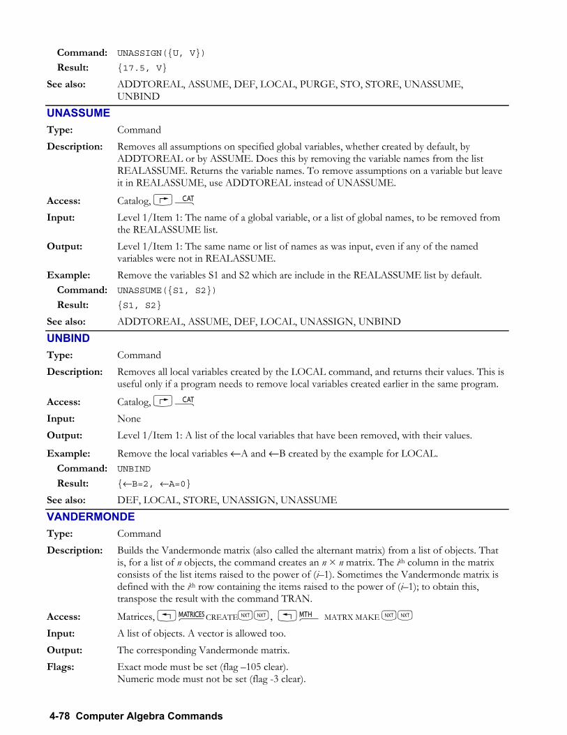
4-78 Computer Algebra Commands
Command: UNASSIGN(U, V)
Result: 17.5, V
See also: ADDTOREAL, ASSUME, DEF, LOCAL, PURGE, STO, STORE, UNASSUME, UNBIND
UNASSUME Type: Command Description: Removes all assumptions on specified global variables, whether created by default, by
ADDTOREAL or by ASSUME. Does this by removing the variable names from the list REALASSUME. Returns the variable names. To remove assumptions on a variable but leave it in REALASSUME, use ADDTOREAL instead of UNASSUME.
Access: Catalog, µ Input: Level 1/Item 1: The name of a global variable, or a list of global names, to be removed from
the REALASSUME list. Output: Level 1/Item 1: The same name or list of names as was input, even if any of the named
variables were not in REALASSUME. Example: Remove the variables S1 and S2 which are include in the REALASSUME list by default.
Command: UNASSUME(S1, S2)
Result: S1, S2
See also: ADDTOREAL, ASSUME, DEF, LOCAL, UNASSIGN, UNBIND
UNBIND Type: Command Description: Removes all local variables created by the LOCAL command, and returns their values. This is
useful only if a program needs to remove local variables created earlier in the same program.
Access: Catalog, µ Input: None Output: Level 1/Item 1: A list of the local variables that have been removed, with their values.
Example: Remove the local variables ←A and ←B created by the example for LOCAL. Command: UNBIND
Result: ←B=2, ←A=0
See also: DEF, LOCAL, STORE, UNASSIGN, UNASSUME
VANDERMONDE Type: Command Description: Builds the Vandermonde matrix (also called the alternant matrix) from a list of objects. That
is, for a list of n objects, the command creates an n × n matrix. The ith column in the matrix consists of the list items raised to the power of (i1). Sometimes the Vandermonde matrix is defined with the ith row containing the items raised to the power of (i1); to obtain this, transpose the result with the command TRAN.
Access: Matrices, !Ø CREATELL, !´ MATRX MAKE LL Input: A list of objects. A vector is allowed too. Output: The corresponding Vandermonde matrix. Flags: Exact mode must be set (flag 105 clear).
Numeric mode must not be set (flag -3 clear).
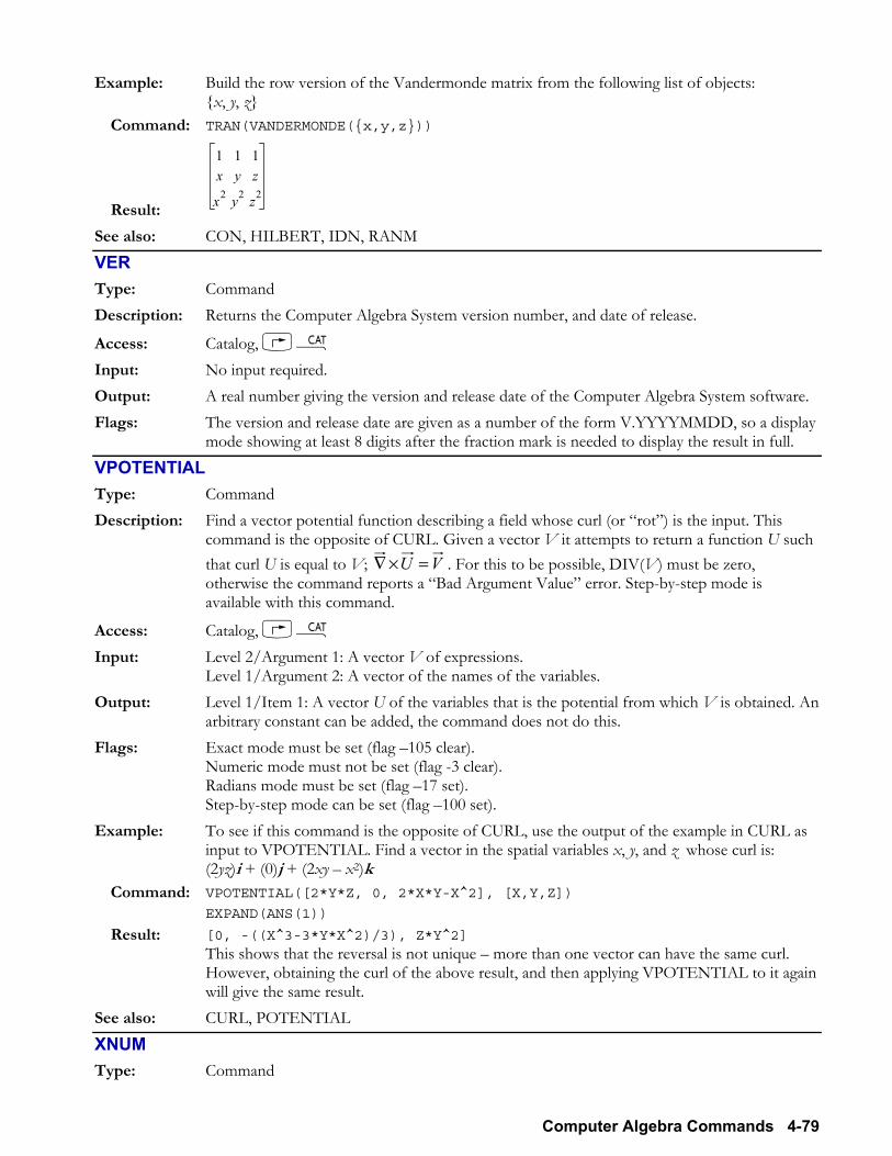
Computer Algebra Commands 4-79
Example: Build the row version of the Vandermonde matrix from the following list of objects: x, y, z
Command: TRAN(VANDERMONDE(x,y,z))
Result:
1 1 1x y z
x2 y2 z2
See also: CON, HILBERT, IDN, RANM
VER Type: Command Description: Returns the Computer Algebra System version number, and date of release.
Access: Catalog, µ Input: No input required. Output: A real number giving the version and release date of the Computer Algebra System software. Flags: The version and release date are given as a number of the form V.YYYYMMDD, so a display
mode showing at least 8 digits after the fraction mark is needed to display the result in full.
VPOTENTIAL Type: Command Description: Find a vector potential function describing a field whose curl (or rot) is the input. This
command is the opposite of CURL. Given a vector V it attempts to return a function U such that curl U is equal to V; VU =×∇ . For this to be possible, DIV(V) must be zero, otherwise the command reports a Bad Argument Value error. Step-by-step mode is available with this command.
Access: Catalog, µ Input: Level 2/Argument 1: A vector V of expressions.
Level 1/Argument 2: A vector of the names of the variables. Output: Level 1/Item 1: A vector U of the variables that is the potential from which V is obtained. An
arbitrary constant can be added, the command does not do this. Flags: Exact mode must be set (flag 105 clear).
Numeric mode must not be set (flag -3 clear). Radians mode must be set (flag 17 set). Step-by-step mode can be set (flag 100 set).
Example: To see if this command is the opposite of CURL, use the output of the example in CURL as input to VPOTENTIAL. Find a vector in the spatial variables x, y, and z whose curl is: (2yz)i + (0)j + (2xy x2)k
Command: VPOTENTIAL([2*Y*Z, 0, 2*X*Y-X^2], [X,Y,Z])
EXPAND(ANS(1))
Result: [0, -((X^3-3*Y*X^2)/3), Z*Y^2] This shows that the reversal is not unique more than one vector can have the same curl. However, obtaining the curl of the above result, and then applying VPOTENTIAL to it again will give the same result.
See also: CURL, POTENTIAL
XNUM Type: Command
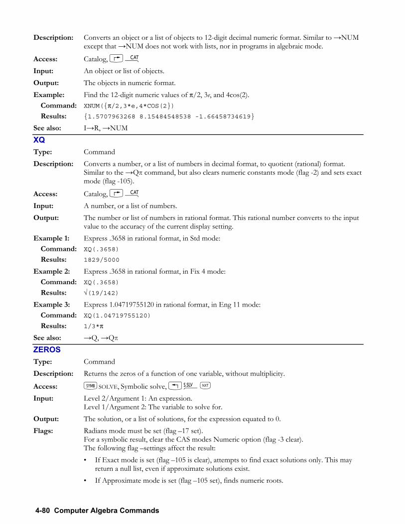
4-80 Computer Algebra Commands
Description: Converts an object or a list of objects to 12-digit decimal numeric format. Similar to →NUM except that →NUM does not work with lists, nor in programs in algebraic mode.
Access: Catalog, µ Input: An object or list of objects. Output: The objects in numeric format. Example: Find the 12-digit numeric values of π/2, 3e, and 4cos(2).
Command: XNUM(π/2,3*e,4*COS(2) Results: 1.5707963268 8.15484548538 -1.66458734619
See also: I→R, →NUM
XQ Type: Command Description: Converts a number, or a list of numbers in decimal format, to quotient (rational) format.
Similar to the →Qπ command, but also clears numeric constants mode (flag -2) and sets exact mode (flag -105).
Access: Catalog, µ Input: A number, or a list of numbers. Output: The number or list of numbers in rational format. This rational number converts to the input
value to the accuracy of the current display setting. Example 1: Express .3658 in rational format, in Std mode:
Command: XQ(.3658)
Results: 1829/5000
Example 2: Express .3658 in rational format, in Fix 4 mode: Command: XQ(.3658)
Results: √(19/142)
Example 3: Express 1.04719755120 in rational format, in Eng 11 mode: Command: XQ(1.04719755120)
Results: 1/3*π
See also: →Q, →Qπ
ZEROS Type: Command Description: Returns the zeros of a function of one variable, without multiplicity.
Access: PSOLVE, Symbolic solve, !ÎL
Input: Level 2/Argument 1: An expression. Level 1/Argument 2: The variable to solve for.
Output: The solution, or a list of solutions, for the expression equated to 0. Flags: Radians mode must be set (flag 17 set).
For a symbolic result, clear the CAS modes Numeric option (flag -3 clear). The following flag settings affect the result: If Exact mode is set (flag 105 is clear), attempts to find exact solutions only. This may
return a null list, even if approximate solutions exist. If Approximate mode is set (flag 105 set), finds numeric roots.
Computer Algebra Commands 4-81
If Complex mode is set (flag 103 set), searches for real and complex roots. Example: Find the roots of the following equation in x, without specifying that x=2 is a root twice.
x3 x2 8x + 12 = 0: Command: ZEROS(X^3-X^2-8*X+12)
Results: -3, 2
? Type: Function Description: The undefined symbol. Used to signify a numeric result that is not defined by the rules of
arithmetic, such as the result of dividing zero by zero, or infinity by infinity. Mathematical operations on ? return ? as a result. Can be used in programs to check for an earlier undefined operation. This use of ? is unrelated to the use of ? as a spare unit in the units system. The unit ? can be used to create new units based on it, units that can not be expressed in terms of other base units. For example you could define $=1_? Then other currencies could be defined as multiples or fractions of 1_? The calculator has symbols for Yen, Pounds and Euros; other currencies could be defined using their names. The unit conversion system would then check conversions between them for consistency because ? is recognized as a base unit.
Access: Catalog, µ, or ~3
∞ Type: Function Description: Infinity: used to signify a numeric result that is infinite by the rules of arithmetic, such as the
result of dividing a non-zero number by zero. The calculator recognizes two kinds of infinity: signed and unsigned. Evaluating '1/0' gives an unsigned infinity '∞'. Selecting infinity from the keyboard, from the CHARS table, or from the catalog µ returns '+∞' and the sign can be changed. Calculations with the unsigned infinity return unsigned infinity or ? as their result. Calculations with the signed infinity can return ordinary numeric results, as in the example. Positive infinity and unsigned infinity are equal if tested with ==, but are not identical if tested with SAME.
Access: Keyboard, CHARS, or catalog, µ
Flags: Exact mode must be set (flag 105 clear), and numeric mode must not be set (flag -3 clear) for mathematical operations to give ∞ as a result, and for executing ∞ from the keyboard or catalog to give +∞ and not an error.
Example: Find the arc tangent of minus infinity. Assume that radians mode is set. Command: ATAN(-∞)
Results: -(π/2)

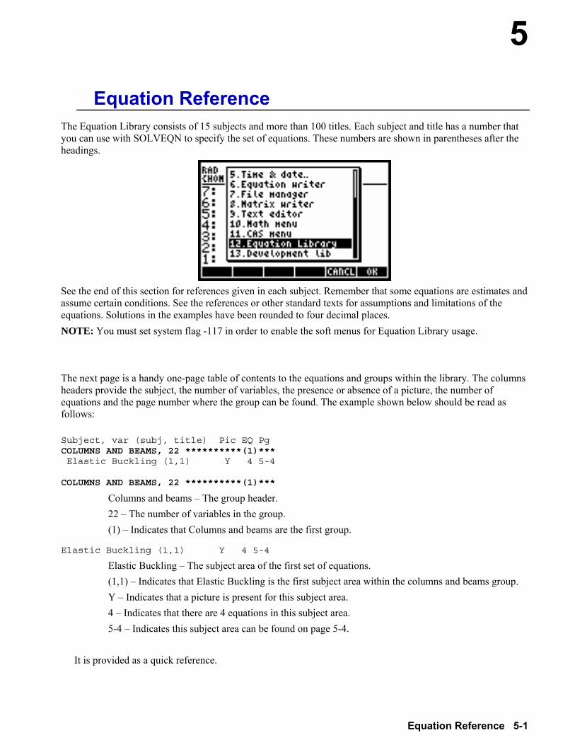
5
Equation Reference 5-1
5.Equation Reference The Equation Library consists of 15 subjects and more than 100 titles. Each subject and title has a number that you can use with SOLVEQN to specify the set of equations. These numbers are shown in parentheses after the headings.
See the end of this section for references given in each subject. Remember that some equations are estimates and assume certain conditions. See the references or other standard texts for assumptions and limitations of the equations. Solutions in the examples have been rounded to four decimal places. NOTE: You must set system flag -117 in order to enable the soft menus for Equation Library usage. The next page is a handy one-page table of contents to the equations and groups within the library. The columns headers provide the subject, the number of variables, the presence or absence of a picture, the number of equations and the page number where the group can be found. The example shown below should be read as follows: Subject, var (subj, title) Pic EQ Pg COLUMNS AND BEAMS, 22 **********(1)*** Elastic Buckling (1,1) Y 4 5-4 COLUMNS AND BEAMS, 22 **********(1)***
Columns and beams The group header. 22 The number of variables in the group. (1) Indicates that Columns and beams are the first group.
Elastic Buckling (1,1) Y 4 5-4
Elastic Buckling The subject area of the first set of equations. (1,1) Indicates that Elastic Buckling is the first subject area within the columns and beams group. Y Indicates that a picture is present for this subject area. 4 Indicates that there are 4 equations in this subject area. 5-4 Indicates this subject area can be found on page 5-4.
It is provided as a quick reference.
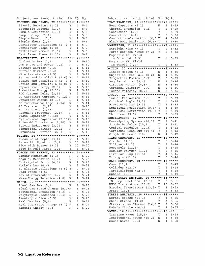
5-2 Equation Reference
Subject, var (subj, title) Pic EQ Pg COLUMNS AND BEAMS, 22 **********(1)***** Elastic Buckling (1,1) Y 4 5-4 Eccentric Columns (1,2) Y 2 5-4 Simple Deflection (1,3) Y 1 5-5 Simple Slope (1,4) Y 1 5-5 Simple Moment (1,5) Y 1 5-6 Simple Shear (1,6) Y 1 5-6 Cantilever Deflection (1,7) Y 1 5-7 Cantilever Slope (1,8) Y 1 5-7 Cantilever Moment (1,9) Y 1 5-8 Cantilever Shear (1,10) Y 1 5-8 ELECTRICITY, 47 ****************(2)***** Coulomb's Law (2,1) N 1 5-10 Ohm's Law and Power (2,2) N 4 5-10 Voltage Divider (2,3) Y 1 5-11 Current Divider (2,4) Y 1 5-11 Wire Resistance (2,5) Y 2 5-11 Series and Parallel R (2,6) Y 2 5-12 Series and Parallel C (2,7) Y 2 5-12 Series and Parallel L (2,8) Y 2 5-13 Capacitive Energy (2,9) N 1 5-13 Inductive Energy (2,10) N 1 5-13 RLC Current Delay (2,11) Y 5 5-14 DC Capacitor Current (2,12) N 3 5-14 Capacitor Charge (2,13) N 1 5-14 DC Inductor Voltage (2,14) N 3 5-14 RC Transient (2,15) Y 1 5-15 RL Transient (2,16) N 1 5-15 Resonant Frequency (2,17) N 4 5-16 Plate Capacitor (2,18) Y 1 5-16 Cylindrical Capacitor (2,19)Y 1 5-16 Solenoid Inductance (2,20) Y 1 5-17 Toroid Inductance (2,21) Y 1 5-17 Sinusoidal Voltage (2,22) N 2 5-18 Sinusoidal Current (2,23) N 2 5-18 FLUIDS, 24 *********************(3)***** Pressure at Depth (3,1) Y 1 5-19 Bernoulli Equation (3,2) Y 10 5-19 Flow with Losses (3,3) Y 10 5-20 Flow in Full Pipes (3,4) Y 8 5-21 FORCES AND ENERGY, 32 **********(4)***** Linear Mechanics (4,1) N 8 5-22 Angular Mechanics (4,2) N 12 5-23 Centripetal Force (4,3) N 4 5-23 Hooke’s Law (4,4) Y 2 5-23 1D Elastic Collisions (4,5) Y 2 5-24 Drag Force (4,6) N 1 5-24 Law of Gravitation (4,7) N 1 5-24 Mass-Energy Relation (4,8) N 1 5-24 GASES, 26 **********************(5)***** Ideal Gas Law (5,1) N 2 5-25 Ideal Gas State Change (5,2)N 1 5-26 Isothermal Expansion (5,3) N 2 5-26 Polytropic Processes (5,4) N 2 5-26 Isentropic Flow (5,5) Y 4 5-26 Real Gas Law (5,6) N 2 5-27 Real Gas State Change (5,7) N 1 5-27 Kinetic Theory (5,8) N 4 5-28
Subject, var (subj, title) Pic EQ Pg HEAT TRANSFER, 23 *************(6)***** Heat Capacity (6,1) N 2 5-29 Thermal Expansion (6,2) Y 2 5-29 Conduction (6,3) Y 2 5-29 Convection (6,4) Y 2 5-30 Conduction+Convection (6,5)Y 4 5-30 Black Body Radiation (6,6) Y 5 5-30 MAGNETISM, 11 *****************(7)***** Straight Wire (7,1) Y 1 5-32 Force between Wires (7,2) Y 1 5-32 Magnetic (B) Field in Solenoid (7,3) Y 1 5-33 Magnetic (B) Field in Toroid (7,4) Y 1 5-33 MOTION, 30 ********************(8)***** Linear Motion (8,1) N 4 5-35 Object in Free Fall (8,2) N 4 5-35 Projectile Motion (8,3) Y 5 5-35 Angular Motion (8,4) N 4 5-36 Circular Motion (8,5) N 3 5-36 Terminal Velocity (8,6) N 1 5-36 Escape Velocity (8,7) N 1 5-36 OPTICS, 10 ********************(9)***** Law of Refraction (9,1) Y 1 5-37 Critical Angle (9,2) Y 1 5-38 Brewster’s Law (9,3) Y 2 5-38 Spherical Reflection (9,4) Y 3 5-39 Spherical Refraction (9,5) Y 1 5-39 Thin Lens (9,6) Y 3 5-39 OSCILLATIONS, 17 *************(10)***** Mass-Spring System (10,1) Y 3 5-41 Simple Pendulum (10,2) Y 3 5-41 Conical Pendulum (10,3) Y 4 5-42 Torsional Pendulum (10,4) Y 3 5-42 Simple Harmonic (10,5) N 4 5-42 PLANE GEOMETRY, 21 ***********(11)***** Circle (11,1) Y 5 5-44 Ellipse (11,2) Y 5 5-44 Rectangle (11,3) Y 5 5-45 Regular Polygon (11,4) Y 6 5-45 Circular Ring (11,5) Y 4 5-46 Triangle (11,6) Y 5 5-46 SOLID GEOMETRY, 12 ***********(12)***** Cone (12,1) Y 5 5-47 Cylinder (12,2) Y 5 5-48 Parallelpiped (12,3) Y 4 5-48 Sphere (12,4) Y 4 5-49 SOLID STATE DEVICES, 60 ******(13)***** PN Step Junctions (13,1) Y 8 5-51 NMOS Transistors (13,2) Y 10 5-52 Bipolar Transistors (13,3) Y 8 5-53 JFETs (13,4) Y 7 5-53 STRESS ANALYSIS, 28 **********(14)***** Normal Stress (14,1) Y 3 5-55 Shear Stress (14,2) Y 3 5-56 Stress on an Element (14,3)Y 3 5-56 Mohr’s Circle (14,4) Y 7 5-57 WAVES, 16 ********************(15)*** Traverse Waves (15,1) Y 4 5-58 Longitudinal Waves (15,2) N 4 5-58 Sound Waves (15,3) N 4 5-58
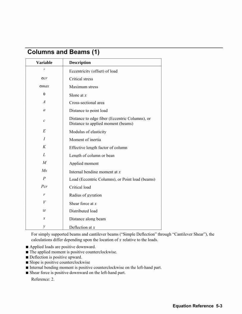
Equation Reference 5-3
Columns and Beams (1) Variable Description
º Eccentricity (offset) of loadσcr Critical stress
σmax Maximum stress
θ Slope at x A Cross-sectional areaa Distance to point load
c Distance to edge fiber (Eccentric Columns), or Distance to applied moment (beams)
E Modulus of elasticityI Moment of inertiaK Effective length factor of columnL Length of column or beanM Applied momentMx Internal bending moment at xP Load (Eccentric Columns), or Point load (beams)
Pcr Critical load r Radius of gyrationV Shear force at x w Distributed loadx Distance along beamy Deflection at x
For simply supported beams and cantilever beams (Simple Deflection through Cantilever Shear), the calculations differ depending upon the location of x relative to the loads.
! Applied loads are positive downward. ! The applied moment is positive counterclockwise. ! Deflection is positive upward. ! Slope is positive counterclockwise ! Internal bending moment is positive counterclockwise on the left-hand part. ! Shear force is positive downward on the left-hand part.
Reference: 2.
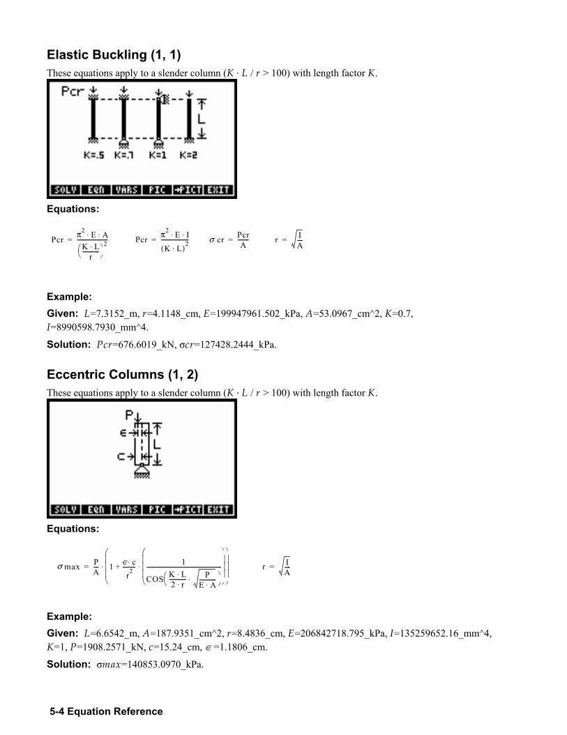
5-4 Equation Reference
Elastic Buckling (1, 1) These equations apply to a slender column (K · L / r > 100) with length factor K.
Equations:
Example: Given: L=7.3152_m, r=4.1148_cm, E=199947961.502_kPa, A=53.0967_cm^2, K=0.7, I=8990598.7930_mm^4.
Solution: Pcr=676.6019_kN, σcr=127428.2444_kPa.
Eccentric Columns (1, 2) These equations apply to a slender column (K · L / r > 100) with length factor K.
Equations:
Example: Given: L=6.6542_m, A=187.9351_cm^2, r=8.4836_cm, E=206842718.795_kPa, I=135259652.16_mm^4, K=1, P=1908.2571_kN, c=15.24_cm, ∈ =1.1806_cm.
Solution: σmax=140853.0970_kPa.
P c r π 2 E A ⋅ ⋅ K L⋅
r - - - - - - - - - - - - ⎝ ⎠ ⎛ ⎞ 2 - - - - - - - - - - - - - - - - - - - - - - = P c r π 2 E I ⋅ ⋅
K L⋅ ( ) 2 - - - - - -- - - - - - - - - - - - - - = σ c r Pcr
A--------= r I
A----=
σ m a x P A - - - - 1 ∈ c ⋅
r 2 - - - - - - - - - + 1
C O S K L ⋅ 2 r ⋅ - - - - - - - - - - - - P
E A ⋅ - - - - - - - - - - - - ⋅ ⎝ ⎠ ⎛ ⎞
- - - - - - - - - - - - - - - - - - - - - - - - - - - - - - - - - - - - - - - - - - - - - - - - - - - - - - ⎝ ⎠ ⎜ ⎟ ⎜ ⎟ ⎜ ⎟ ⎛ ⎞
⋅ ⎝ ⎠⎜ ⎟⎜ ⎟⎜ ⎟⎛ ⎞
⋅ = r IA----=
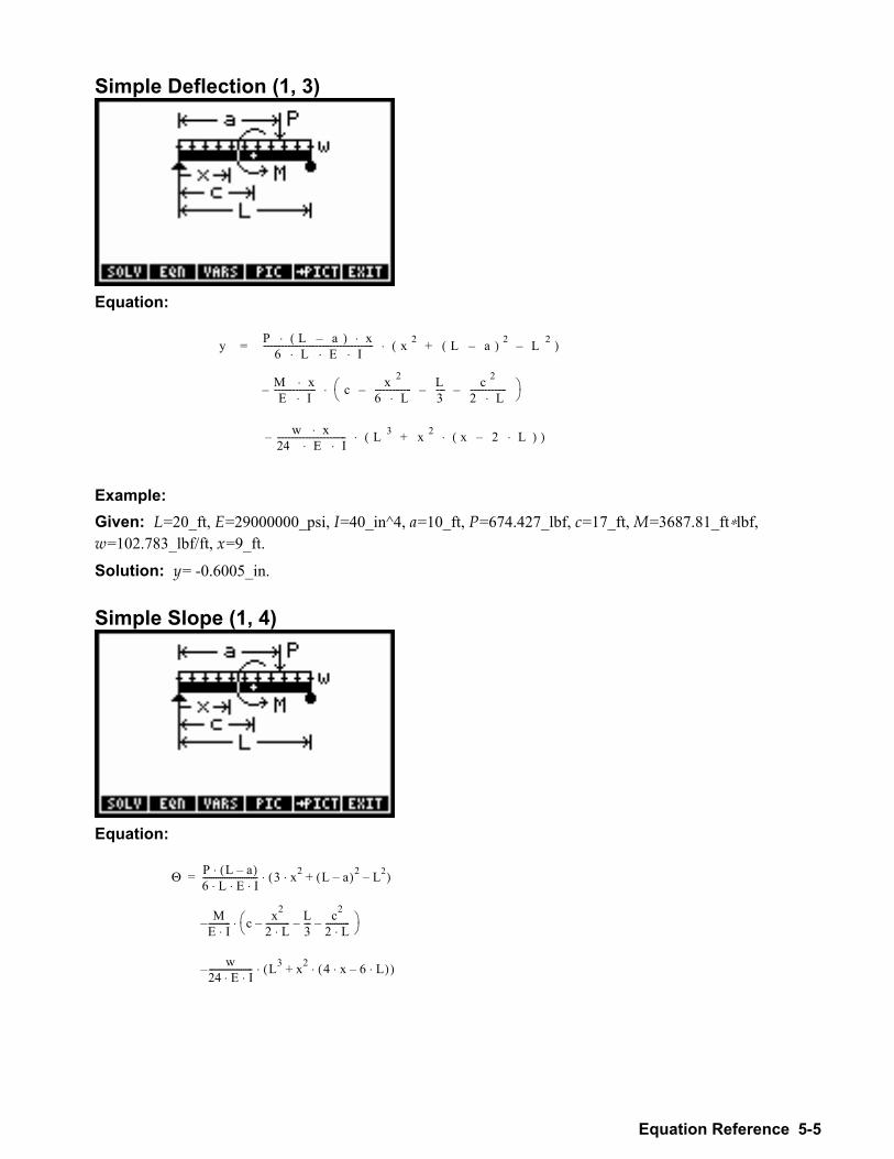
Equation Reference 5-5
Simple Deflection (1, 3)
Equation:
y P L a( ) x⋅ ⋅6 L E I⋅ ⋅ ⋅
-------------------------------- x 2 L a( ) 2 L 2+( )⋅=
M x⋅E I⋅
------------ c x 2
6 L⋅----------- L
3--- c 2
2 L⋅-----------⎝ ⎠
⎛ ⎞⋅
w x⋅24 E I⋅ ⋅-------------------- L 3 x 2 x 2 L⋅( )⋅+( )⋅
Example: Given: L=20_ft, E=29000000_psi, I=40_in^4, a=10_ft, P=674.427_lbf, c=17_ft, M=3687.81_ft∗lbf, w=102.783_lbf/ft, x=9_ft.
Solution: y= -0.6005_in.
Simple Slope (1, 4)
Equation:
Θ P L a( )⋅6 L E I⋅ ⋅ ⋅------------------------- 3 x⋅ 2 L a( )2 L2+( )⋅=
ME I⋅---------- c x2
2 L⋅----------- L
3--- c2
2 L⋅-----------⎝ ⎠
⎛ ⎞⋅
w24 E I⋅ ⋅-------------------- L3 x2 4 x⋅ 6 L⋅( )⋅+( )⋅
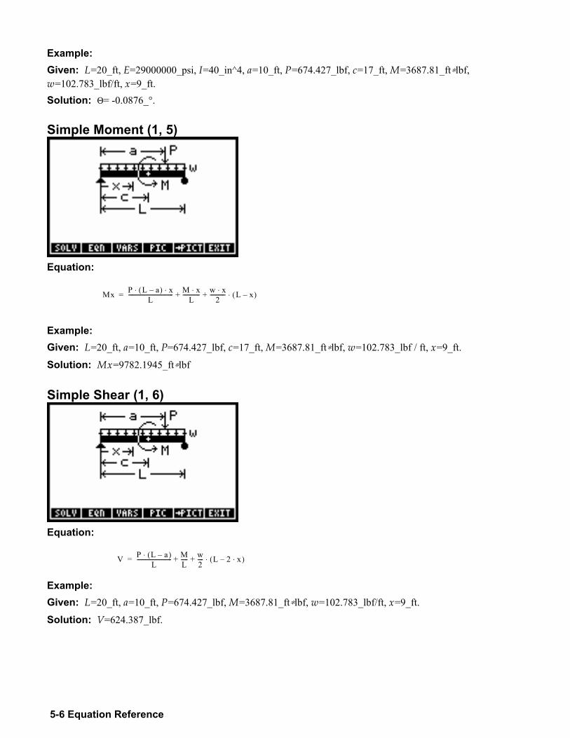
5-6 Equation Reference
Example: Given: L=20_ft, E=29000000_psi, I=40_in^4, a=10_ft, P=674.427_lbf, c=17_ft, M=3687.81_ft∗lbf, w=102.783_lbf/ft, x=9_ft. Solution: Θ= -0.0876_°.
Simple Moment (1, 5)
Equation:
Mx P L a( ) x⋅ ⋅L
-------------------------------- M x⋅L
------------ w x⋅2
-----------+ L x( )⋅+=
Example: Given: L=20_ft, a=10_ft, P=674.427_lbf, c=17_ft, M=3687.81_ft∗lbf, w=102.783_lbf / ft, x=9_ft.
Solution: Mx=9782.1945_ft∗lbf
Simple Shear (1, 6)
Equation:
V P L a( )⋅L
------------------------- ML----- w
2----+ L 2 x⋅( )⋅+=
Example: Given: L=20_ft, a=10_ft, P=674.427_lbf, M=3687.81_ft∗lbf, w=102.783_lbf/ft, x=9_ft.
Solution: V=624.387_lbf.
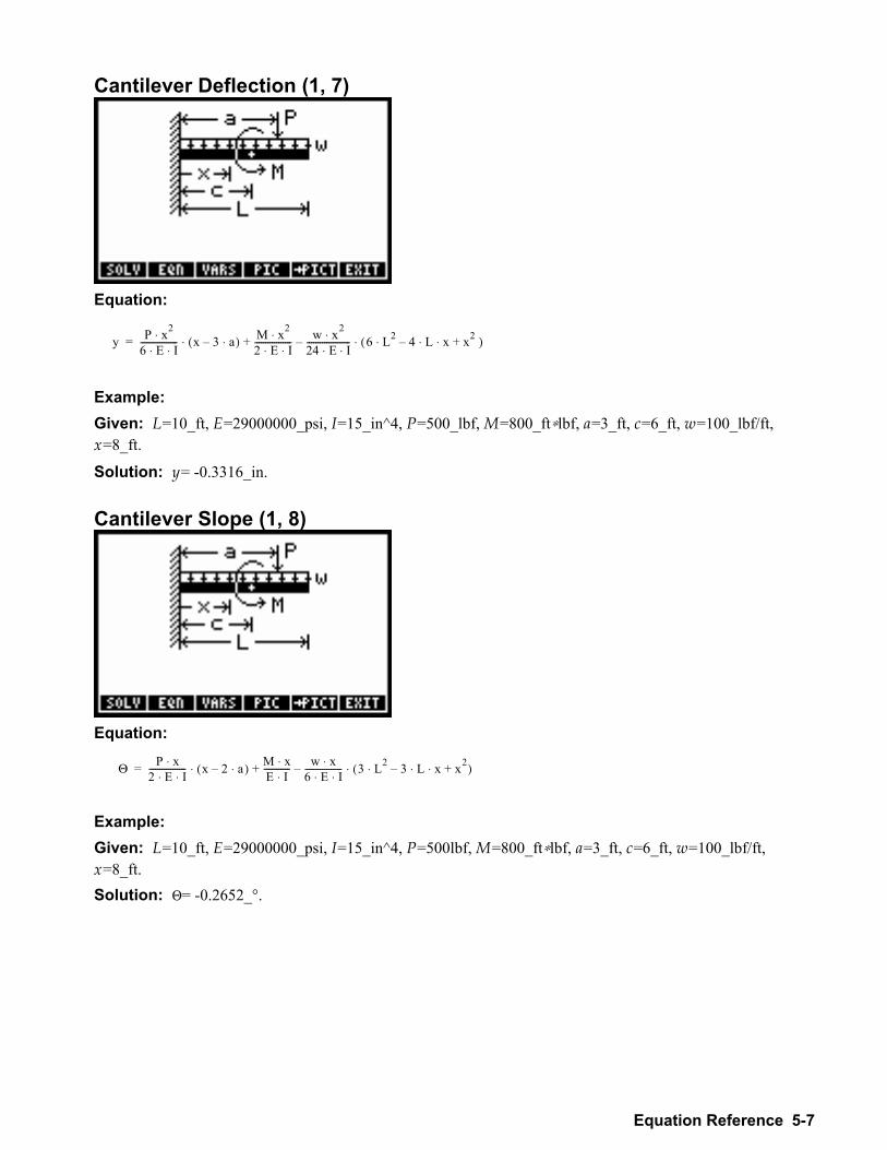
Equation Reference 5-7
Cantilever Deflection (1, 7)
Equation:
y P x2⋅6 E I⋅ ⋅----------------- x 3 a⋅( )⋅ M x2⋅
2 E I⋅ ⋅----------------- w x2⋅
24 E I⋅ ⋅-------------------- 6 L2⋅ 4 L x⋅ ⋅ x2+( )⋅+=
Example: Given: L=10_ft, E=29000000_psi, I=15_in^4, P=500_lbf, M=800_ft∗lbf, a=3_ft, c=6_ft, w=100_lbf/ft, x=8_ft.
Solution: y= -0.3316_in.
Cantilever Slope (1, 8)
Equation:
Θ P x⋅2 E I⋅ ⋅----------------- x 2 a⋅( )⋅ M x⋅
E I⋅------------ w x⋅
6 E I⋅ ⋅----------------- 3 L2⋅ 3 L x⋅ ⋅ x2+( )⋅+=
Example: Given: L=10_ft, E=29000000_psi, I=15_in^4, P=500lbf, M=800_ft∗lbf, a=3_ft, c=6_ft, w=100_lbf/ft, x=8_ft. Solution: Θ= -0.2652_°.
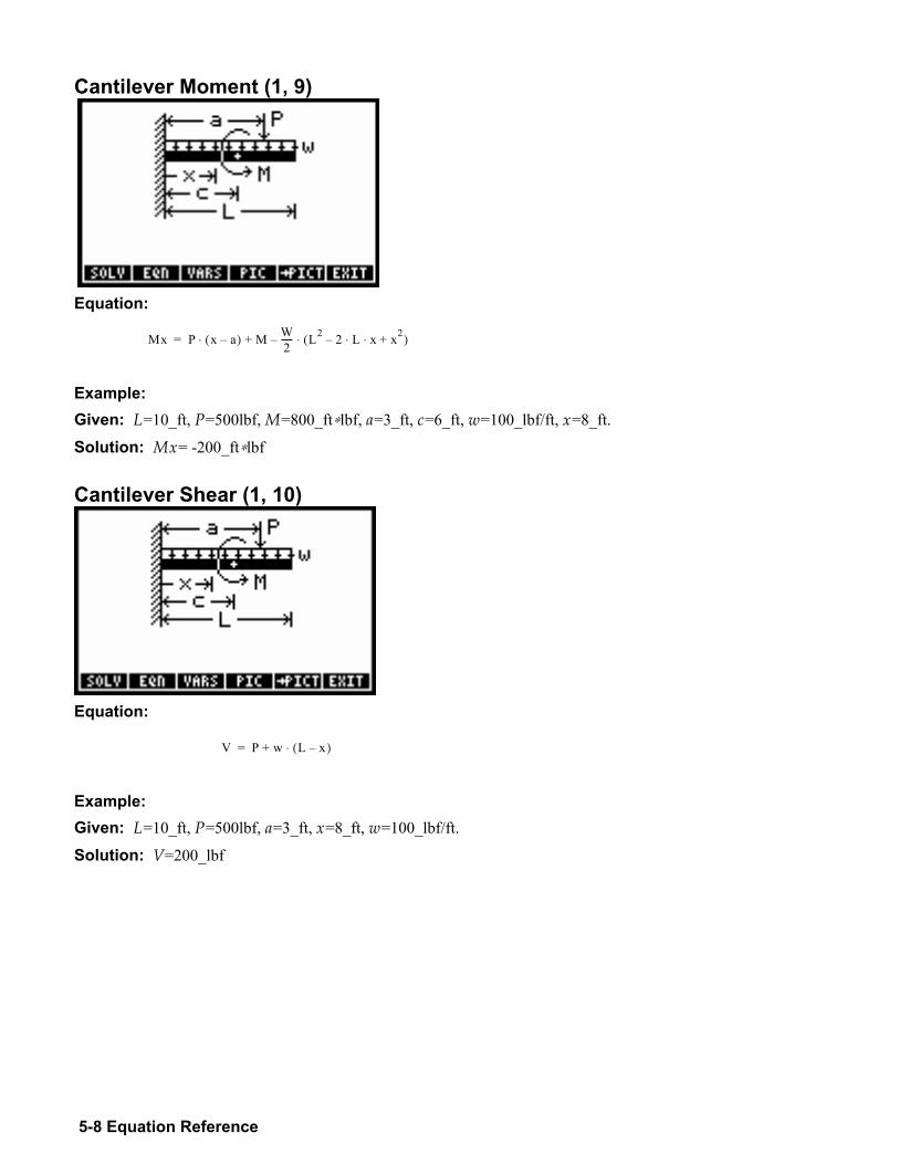
5-8 Equation Reference
Cantilever Moment (1, 9)
Equation:
Mx P x a( )⋅ M W2----- L2 2 L x⋅ ⋅ x2+( )⋅+=
Example: Given: L=10_ft, P=500lbf, M=800_ft∗lbf, a=3_ft, c=6_ft, w=100_lbf/ft, x=8_ft.
Solution: Mx= -200_ft∗lbf
Cantilever Shear (1, 10)
Equation:
V P w L x( )⋅+=
Example: Given: L=10_ft, P=500lbf, a=3_ft, x=8_ft, w=100_lbf/ft.
Solution: V=200_lbf
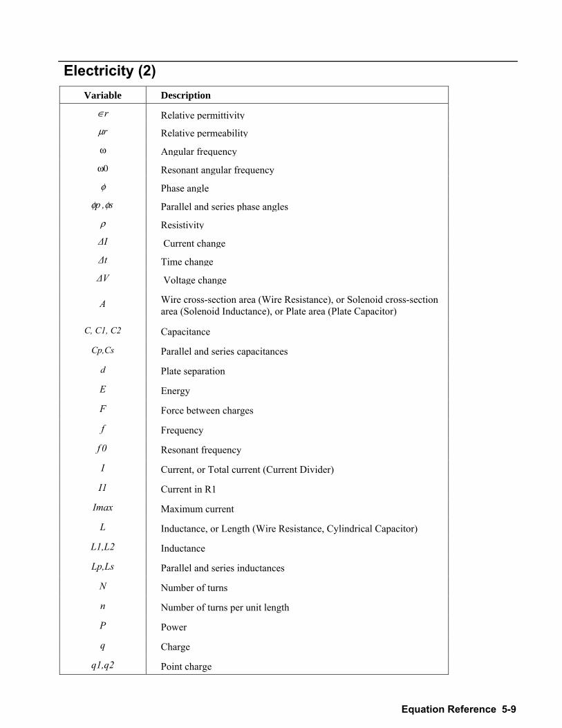
Equation Reference 5-9
Electricity (2) Variable Description
∈r Relative permittivityµr Relative permeability
ω Angular frequency
ω0 Resonant angular frequency
φ Phase angle φp ,φs Parallel and series phase angles
ρ Resistivity ∆I Current change ∆t Time change ∆V Voltage change
A Wire cross-section area (Wire Resistance), or Solenoid cross-section area (Solenoid Inductance), or Plate area (Plate Capacitor)
C, C1, C2 Capacitance
Cp,Cs Parallel and series capacitances
d Plate separation
E Energy
F Force between charges
f Frequency
f 0 Resonant frequency
I Current, or Total current (Current Divider)
I1 Current in R1
Imax Maximum current
L Inductance, or Length (Wire Resistance, Cylindrical Capacitor)
L1,L2 Inductance
Lp,Ls Parallel and series inductances
N Number of turns
n Number of turns per unit length
P Power
q Charge
q1,q2 Point charge
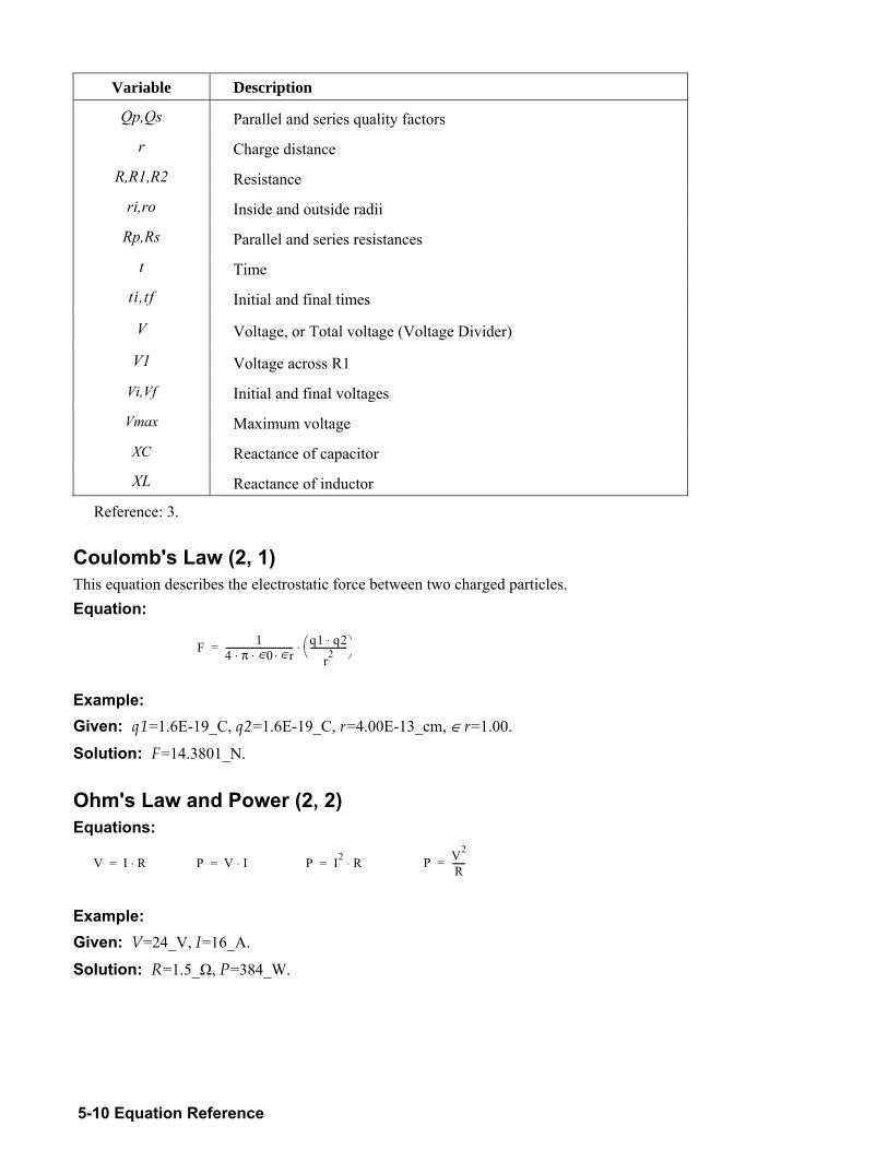
5-10 Equation Reference
Variable Description
Qp,Qs Parallel and series quality factors
r Charge distance
R,R1,R2 Resistance
ri,ro Inside and outside radii
Rp,Rs Parallel and series resistances
t Time
ti,tf Initial and final times
V Voltage, or Total voltage (Voltage Divider)
V1 Voltage across R1
Vi,Vf Initial and final voltages
Vmax Maximum voltage
XC Reactance of capacitor
XL Reactance of inductor
Reference: 3.
Coulomb's Law (2, 1) This equation describes the electrostatic force between two charged particles. Equation:
Example: Given: q1=1.6E-19_C, q2=1.6E-19_C, r=4.00E-13_cm, ∈ r=1.00.
Solution: F=14.3801_N.
Ohm's Law and Power (2, 2) Equations:
V I R⋅= P V I⋅= P I2 R⋅= P V2
R------=
Example: Given: V=24_V, I=16_A.
Solution: R=1.5_Ω, P=384_W.
F 1 4 π ∈0 ∈ r ⋅ ⋅ ⋅ - - - - - - - - - - - - - - - - - - - - - - - - - - - - - - - q 1 q 2 ⋅
r 2 - - - - - - - - - - - - - - - - - ⎝ ⎠ ⎛ ⎞ ⋅ =
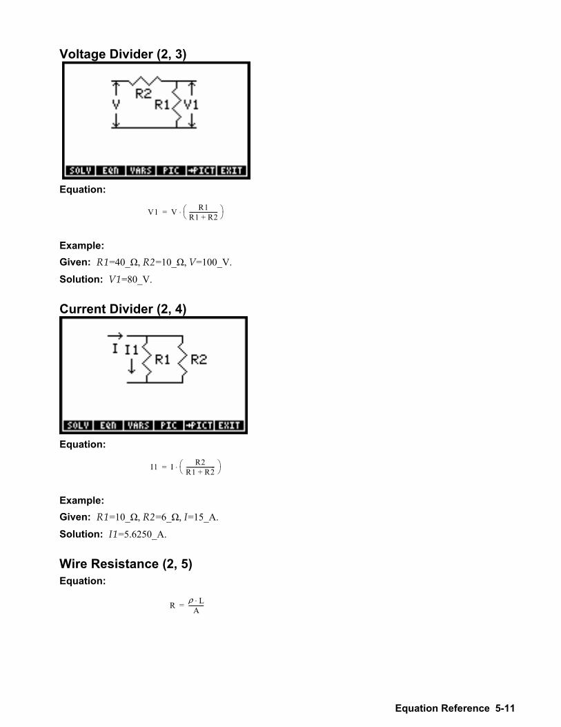
Equation Reference 5-11
Voltage Divider (2, 3)
Equation:
V1 V R1R1 R2+---------------------⎝ ⎠
⎛ ⎞⋅=
Example: Given: R1=40_Ω, R2=10_Ω, V=100_V.
Solution: V1=80_V.
Current Divider (2, 4)
Equation:
I1 I R2R1 R2+---------------------⎝ ⎠
⎛ ⎞⋅=
Example: Given: R1=10_Ω, R2=6_Ω, I=15_A.
Solution: I1=5.6250_A.
Wire Resistance (2, 5) Equation:
R ρ L ⋅ A - - - - - - - - - - - =
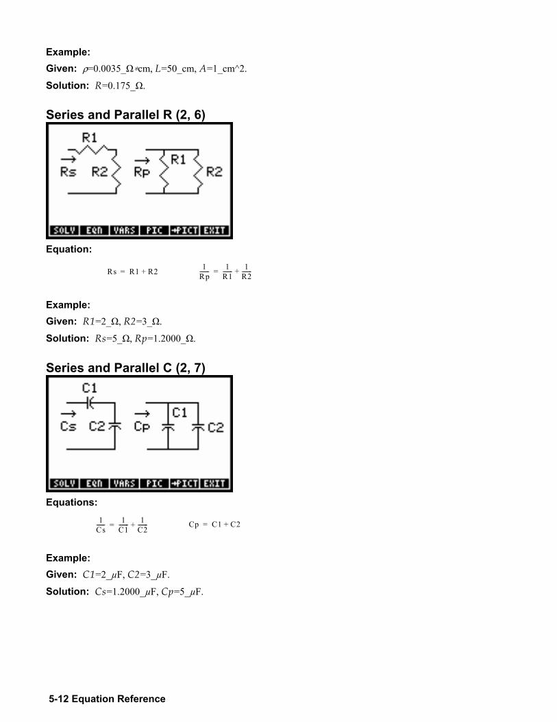
5-12 Equation Reference
Example: Given: ρ=0.0035_Ω∗cm, L=50_cm, A=1_cm^2.
Solution: R=0.175_Ω. Series and Parallel R (2, 6)
Equation:
Rs R1 R2+= 1Rp------- 1
R1------- 1
R2-------+=
Example: Given: R1=2_Ω, R2=3_Ω.
Solution: Rs=5_Ω, Rp=1.2000_Ω.
Series and Parallel C (2, 7)
Equations:
1Cs------ 1
C1------- 1
C2-------+= Cp C1 C2+=
Example: Given: C1=2_µF, C2=3_µF.
Solution: Cs=1.2000_µF, Cp=5_µF.
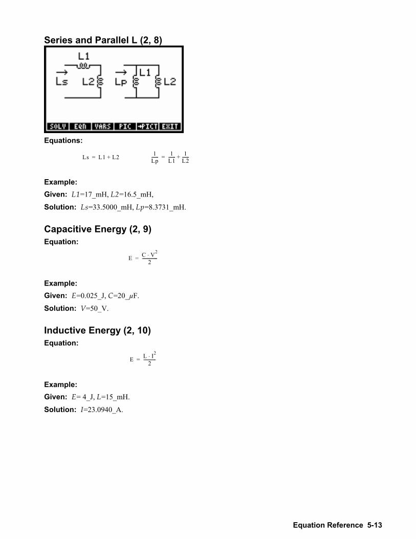
Equation Reference 5-13
Series and Parallel L (2, 8)
Equations:
Ls L1 L2+= 1Lp------- 1
L1------- 1
L2-------+=
Example: Given: L1=17_mH, L2=16.5_mH,
Solution: Ls=33.5000_mH, Lp=8.3731_mH.
Capacitive Energy (2, 9) Equation:
E C V2⋅2
---------------=
Example: Given: E=0.025_J, C=20_µF.
Solution: V=50_V.
Inductive Energy (2, 10) Equation:
E L I2⋅2
------------=
Example: Given: E= 4_J, L=15_mH.
Solution: I=23.0940_A.
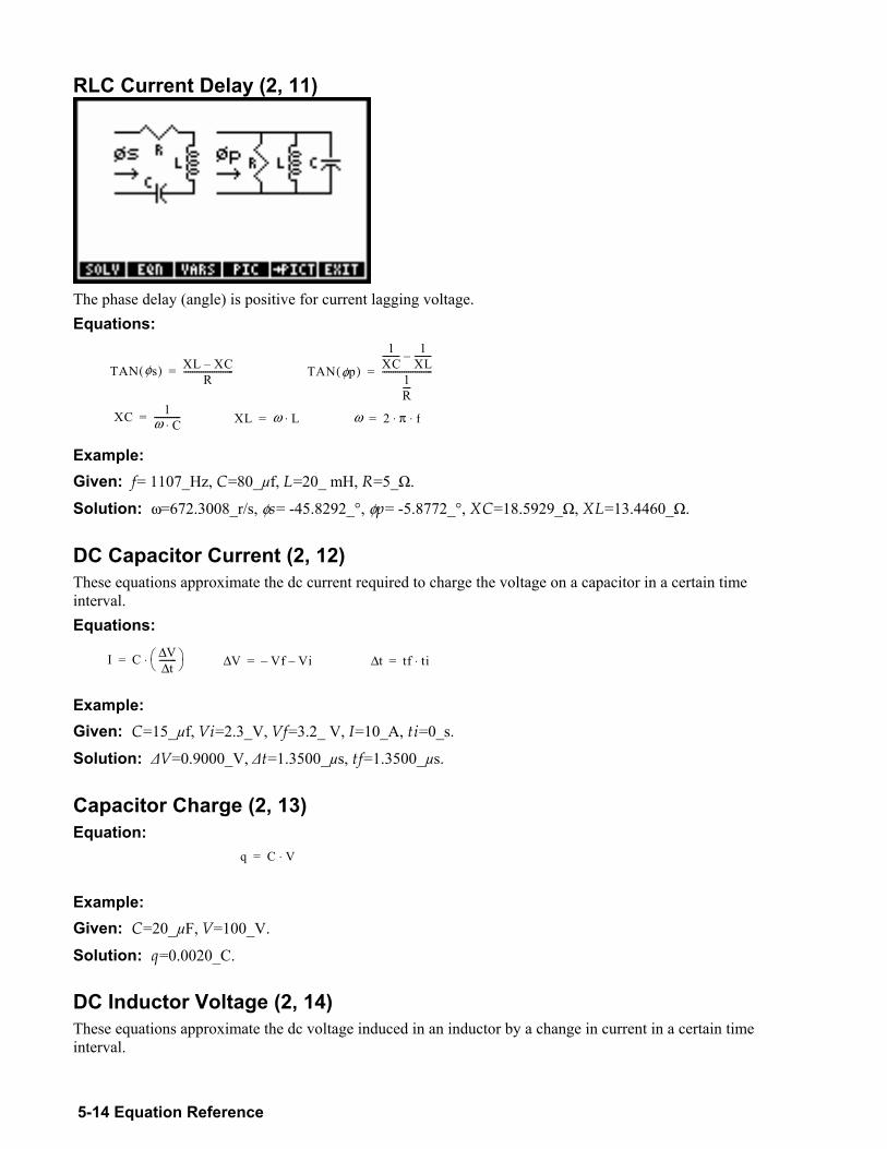
5-14 Equation Reference
RLC Current Delay (2, 11)
The phase delay (angle) is positive for current lagging voltage. Equations:
Example: Given: f= 1107_Hz, C=80_µf, L=20_ mH, R=5_Ω.
Solution: ω=672.3008_r/s, φs= -45.8292_°, φp= -5.8772_°, XC=18.5929_Ω, XL=13.4460_Ω.
DC Capacitor Current (2, 12) These equations approximate the dc current required to charge the voltage on a capacitor in a certain time interval. Equations:
I C V∆t∆
--------⎝ ⎠⎛ ⎞⋅= V∆ Vf Vi= t∆ tf ti⋅=
Example: Given: C=15_µf, Vi=2.3_V, Vf=3.2_ V, I=10_A, ti=0_s.
Solution: ∆V=0.9000_V, ∆t=1.3500_µs, tf=1.3500_µs.
Capacitor Charge (2, 13) Equation:
q C V⋅=
Example: Given: C=20_µF, V=100_V.
Solution: q=0.0020_C. DC Inductor Voltage (2, 14) These equations approximate the dc voltage induced in an inductor by a change in current in a certain time interval.
T A N φ s ( ) X L X C R - - - - - - - - - - - - - - - - - - - - - - - = T A N φ p ( )
1XC-------- 1
XL--------
1R----
-----------------------=
X C 1 ω C ⋅ - - - - - - - - - - - - = X L ω L ⋅ = ω 2 π f⋅ ⋅=
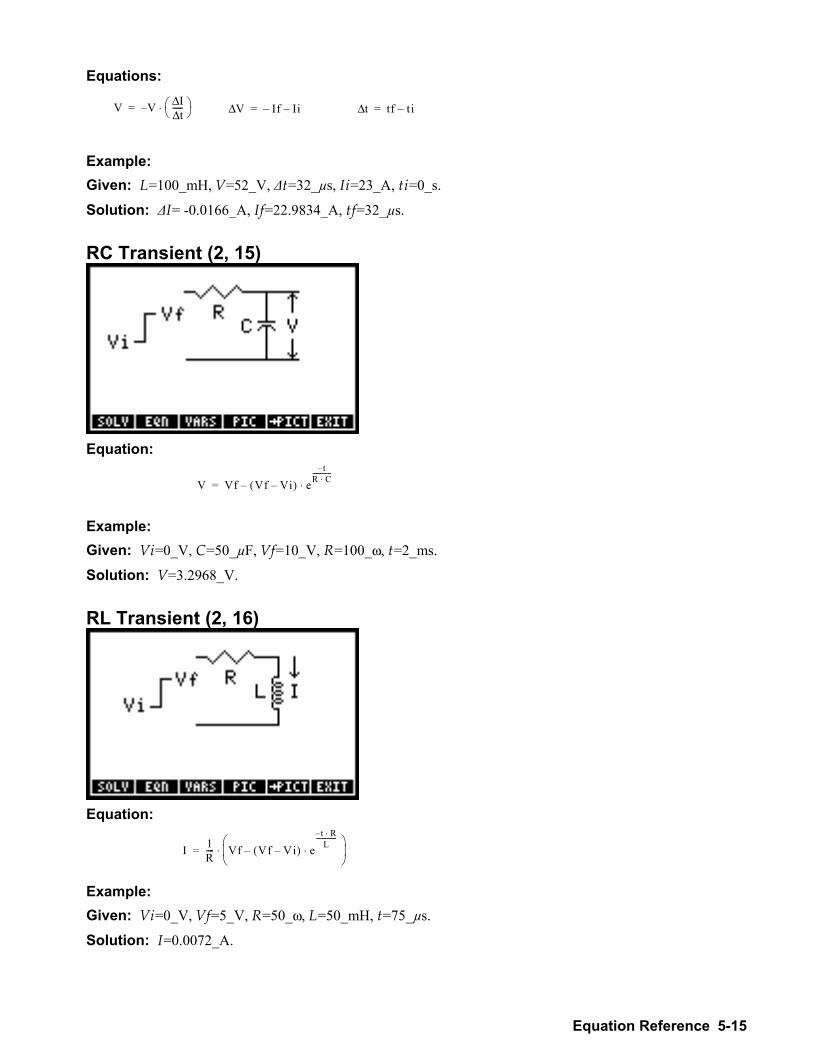
Equation Reference 5-15
Equations:
V V I∆t∆
-----⎝ ⎠⎛ ⎞⋅= V∆ If Ii= t∆ tf ti=
Example: Given: L=100_mH, V=52_V, ∆t=32_µs, Ii=23_A, ti=0_s.
Solution: ∆I= -0.0166_A, If=22.9834_A, tf=32_µs.
RC Transient (2, 15)
Equation:
V Vf Vf Vi( ) et
R C⋅------------
⋅=
Example: Given: Vi=0_V, C=50_µF, Vf=10_V, R=100_ω, t=2_ms.
Solution: V=3.2968_V.
RL Transient (2, 16)
Equation:
I 1R---- Vf Vf Vi( ) e
t R⋅L
-------------⋅
⎝ ⎠⎜ ⎟⎛ ⎞
⋅=
Example: Given: Vi=0_V, Vf=5_V, R=50_ω, L=50_mH, t=75_µs.
Solution: I=0.0072_A.
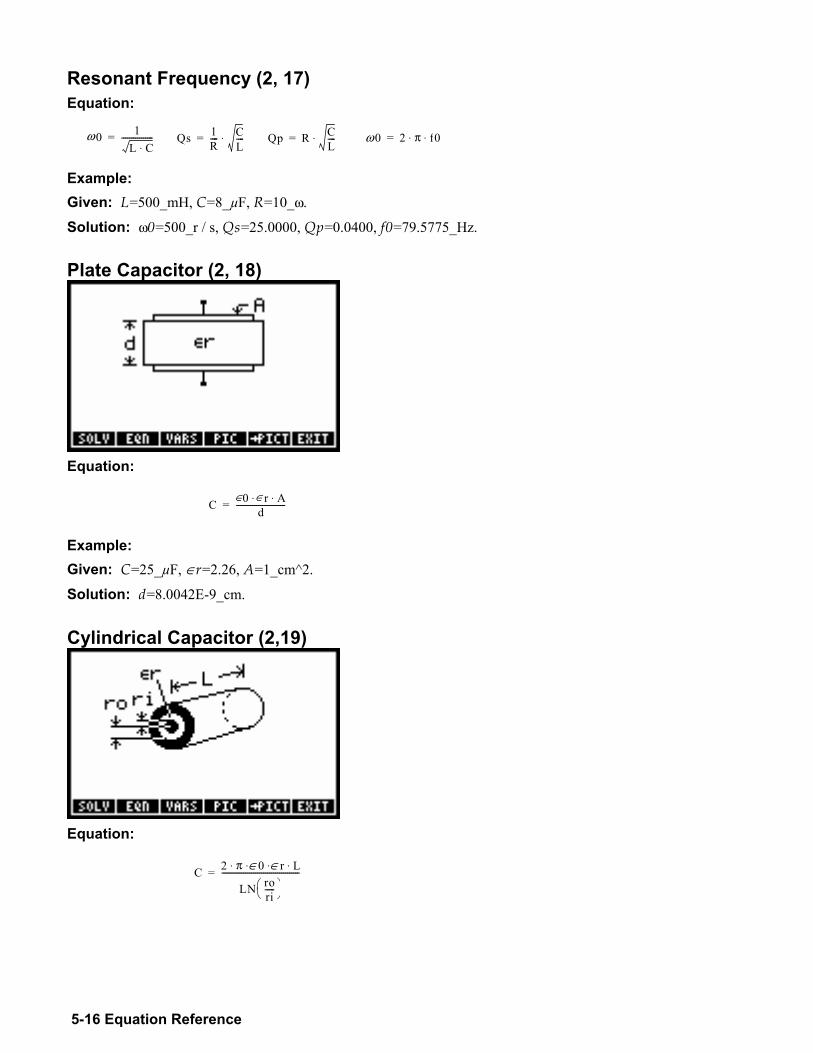
5-16 Equation Reference
Resonant Frequency (2, 17) Equation:
Example: Given: L=500_mH, C=8_µF, R=10_ω.
Solution: ω0=500_r / s, Qs=25.0000, Qp=0.0400, f0=79.5775_Hz.
Plate Capacitor (2, 18)
Equation:
Example: Given: C=25_µF, ∈r=2.26, A=1_cm^2.
Solution: d=8.0042E-9_cm. Cylindrical Capacitor (2,19)
Equation:
ω 0 1 L C ⋅
- - - - - - - - - - - - - - - - = Q s 1 R - - - - C
L - - - - ⋅ = Q p R CL----⋅ = ω 0 2 π f0⋅ ⋅=
C ∈ 0 ∈ r A ⋅ ⋅ d - - - - - - - - - - - - - - - - - - - - - - - - - =
C 2 π ∈ 0 ∈ r L ⋅ ⋅ ⋅ ⋅
LN r o r i - - - - - ⎝ ⎠
⎛ ⎞ - - - - - - - - - - -- - - - - - - - - - - - - - - - - - - - - - - - - - - - =
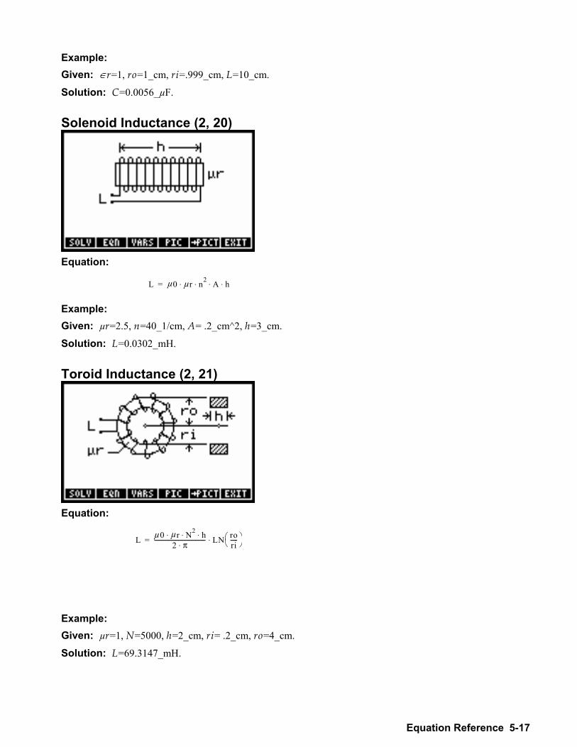
Equation Reference 5-17
Example: Given: ∈r=1, ro=1_cm, ri=.999_cm, L=10_cm.
Solution: C=0.0056_µF.
Solenoid Inductance (2, 20)
Equation:
Example: Given: µr=2.5, n=40_1/cm, A= .2_cm^2, h=3_cm.
Solution: L=0.0302_mH.
Toroid Inductance (2, 21)
Equation:
Example: Given: µr=1, N=5000, h=2_cm, ri= .2_cm, ro=4_cm.
Solution: L=69.3147_mH.
L µ 0 µ r n 2 A h ⋅ ⋅ ⋅ ⋅ =
L µ 0 µ r N 2 h ⋅ ⋅ ⋅ 2 π ⋅ - - - - - - - - - - - - -- - - - - - - - - - - - - - - - - - - - - - - L N ro
ri-----⎝ ⎠
⎛ ⎞⋅ =
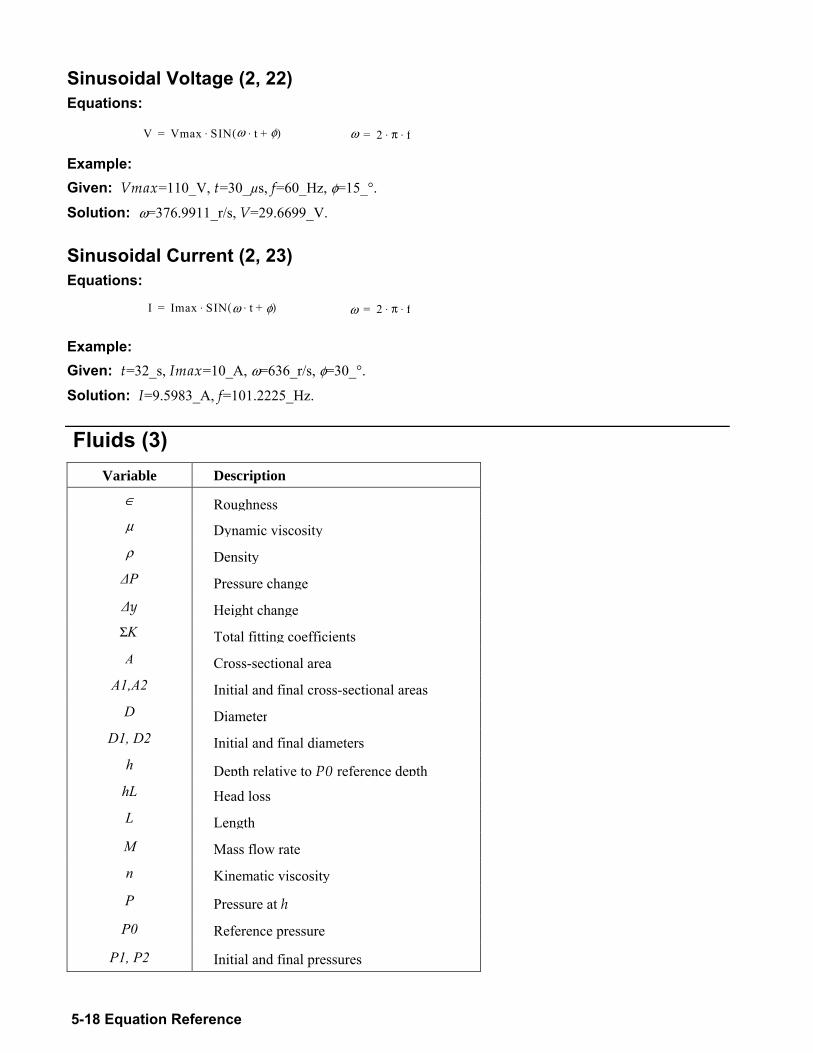
5-18 Equation Reference
Sinusoidal Voltage (2, 22) Equations:
Example: Given: Vmax=110_V, t=30_µs, f=60_Hz, φ=15_°.
Solution: ω=376.9911_r/s, V=29.6699_V.
Sinusoidal Current (2, 23) Equations:
Example: Given: t=32_s, Imax=10_A, ω=636_r/s, φ=30_°.
Solution: I=9.5983_A, f=101.2225_Hz.
Fluids (3) Variable Description
∈ Roughness µ Dynamic viscosity ρ Density ∆P Pressure change ∆y Height change ΣK Total fitting coefficientsA Cross-sectional area
A1,A2 Initial and final cross-sectional areasD Diameter
D1, D2 Initial and final diametersh Depth relative to P0 reference depth
hL Head loss L Length M Mass flow rate n Kinematic viscosity
P Pressure at h
P0 Reference pressure
P1, P2 Initial and final pressures
V V m ax S I N ω t ⋅ φ + ( ) ⋅ = ω 2 π f⋅ ⋅=
I I m a x S I N ω t ⋅ φ + ( ) ⋅ = ω
2 π f⋅ ⋅=
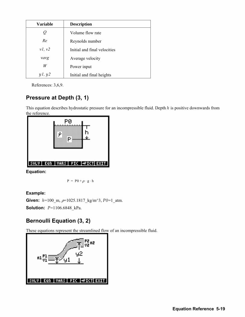
Equation Reference 5-19
Variable Description
Q Volume flow rate
Re Reynolds number
v1, v2 Initial and final velocities
vavg Average velocity
W Power input
y1, y2 Initial and final heights
References: 3,6,9.
Pressure at Depth (3, 1)
This equation describes hydrostatic pressure for an incompressible fluid. Depth h is positive downwards from the reference.
Equation:
Example: Given: h=100_m, ρ=1025.1817_kg/m^3, P0=1_atm.
Solution: P=1106.6848_kPa.
Bernoulli Equation (3, 2) These equations represent the streamlined flow of an incompressible fluid.
P P 0 ρ g h ⋅ ⋅ + =
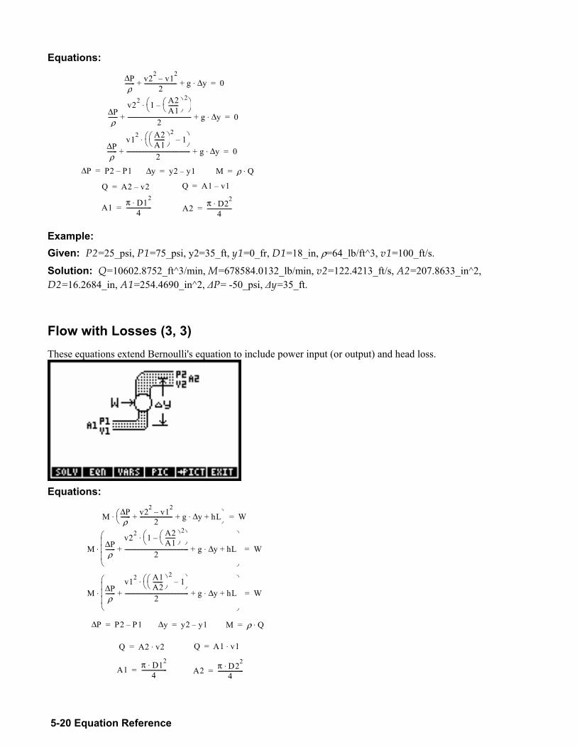
5-20 Equation Reference
Equations: P ∆
ρ - - - - - - - v 2 2 v 1 2 2 - - - - - - - - - - - - - - - - - - - -- - - g + + y ∆ ⋅ 0 =
P ∆ ρ - - - - - - -
v 2 2 1 A 2 A 1 - - -- - - - ⎝ ⎠ ⎛ ⎞ 2 ⎝ ⎠ ⎛ ⎞ ⋅
2 - - - - - - - - - - - - - - - - - - - - - - - - - - - - - - - -- - - - - - - - - - - - - g + + y ∆ ⋅ 0=
P ∆ ρ - - - - - - -
v 1 2 A 2 A 1 - - - - - - - ⎝ ⎠ ⎛ ⎞ 2 1 ⎝ ⎠ ⎛ ⎞ ⋅ 2 - - - - - - - - - - - - - - - - - - - - - - - - - - - - - - - - - - - - - - - - - - - - - g + + y ∆ ⋅ 0=
P ∆ P 2 P 1 = y ∆ y2 y 1 = M ρ Q⋅=
Q A 2 v 2 = Q A 1 v 1 =
A 1 π D 1 2 ⋅ 4 - - - - - - - - - - - - - - - - - - = A 2 π D 2 2⋅
4 - - - - - - - - - - - - - - - - --=
Example: Given: P2=25_psi, P1=75_psi, y2=35_ft, y1=0_fr, D1=18_in, ρ=64_lb/ft^3, v1=100_ft/s.
Solution: Q=10602.8752_ft^3/min, M=678584.0132_lb/min, v2=122.4213_ft/s, A2=207.8633_in^2, D2=16.2684_in, A1=254.4690_in^2, ∆P= -50_psi, ∆y=35_ft.
Flow with Losses (3, 3) These equations extend Bernoulli's equation to include power input (or output) and head loss.
Equations:
M P ∆
ρ - - - - - - - v 2 2 v 1 2 2 - - - - - - - - - - - - - - - - - - - - - - - g + + y ∆ ⋅ h L + ⎝ ⎠ ⎛ ⎞ ⋅ W=
P ∆ P 2 P 1 = y ∆ y 2 y 1 = M ρ Q⋅=
Q A 2 v 2 ⋅ = Q A 1 v1⋅ =
A 1 π D 1 2 ⋅ 4 - - - - - - - - - - - - - - - - - - = A 2 π D22⋅
4- - - - - - - - - ---------=
M P ∆ ρ - - - - - - -
v 2 2 1 A 2 A 1 - - - - -- - ⎝ ⎠ ⎛ ⎞ 2 ⎝ ⎠ ⎛ ⎞ ⋅
2 - - - - - - - - - - - - - - - - - - - - - - - - - - - - - - - - - -- - - - - - - - - - - g + + y ∆ ⋅ h L+ ⎝ ⎠⎜ ⎜ ⎜ ⎛ ⎞
⋅ W=
M P ∆ ρ - - - - - - -
v 1 2 A 1 A 2 - - - - - - - ⎝ ⎠ ⎛ ⎞ 2 1 ⎝ ⎠ ⎛ ⎞ ⋅ 2 - - - - - - - - - - - - - - - - - - - - - - - - - - - - - - - - - -- - - - - - - - - - - g + + y ∆ ⋅ h L+
⎝ ⎠⎜ ⎜ ⎜ ⎛ ⎞
⋅ W=
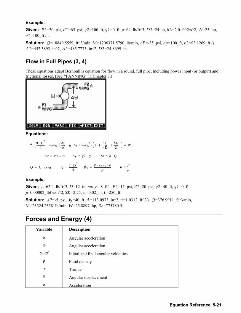
Equation Reference 5-21
Example: Given: P2=30_psi, P1=65_psi, y2=100_ft, y1=0_ft, ρ=64_lb/ft^3, D1=24_in, hL=2.0_ft^2/s^2, W=25_hp, v1=100_ft / s.
Solution: Q=18849.5559_ft^3/min, M=1206371.5790_lb/min, ∆P=-35_psi, ∆y=100_ft, v2=93.1269_ft /s, A1=452.3893_in^2, A2=485.7773_in^2, D2=24.8699_in.
Flow in Full Pipes (3, 4) These equations adapt Bernoulli's equation for flow in a round, full pipe, including power input (or output) and frictional losses. (See FANNING in Chapter 3.)
Equations:
Example: Given: ρ=62.4_lb/ft^3, D=12_in, vavg= 8_ft/s, P2=15_psi, P1=20_psi, y2=40_ft, y1=0_ft, µ=0.00002_lbf∗s/ft^2, ΣK=2.25, ∈=0.02_in, L=250_ft.
Solution: ∆P=-5_psi, ∆y=40_ft, A=113.0973_in^2, n=1.0312_ft^2/s, Q=376.9911_ft^3/min, M=23524.2358_lb/min, W=25.8897_hp, Re=775780.5.
Forces and Energy (4) Variable Description
α Angular accelerationω Angular acceleration
ωi,ωf Initial and final angular velocities
ρ Fluid density τ Torque
Θ Angular displacementα Acceleration
ρ π D 2 ⋅ 4 - - - - - - - - - - - - - - ⎝ ⎠
⎛ ⎞ v a v g P ∆ ρ - - - - - - - g + y ∆⋅ v a v g 2 + 2 f L
D----⎝ ⎠
⎛ ⎞⋅ ⋅ ΣK2
--------+⎝ ⎠⎛ ⎞⋅ ⎝ ⎠
⎛ ⎞⋅ ⋅ ⋅ W=
P ∆ P 2 P 1 = y ∆ y 2 y 1 = M ρ Q⋅=
Q A v a v g ⋅ = n µρ---=A π D 2 ⋅
4 - - - - -- - - - - - - - - = R e D vavg ρ⋅ ⋅µ
- - - - -------------------------=
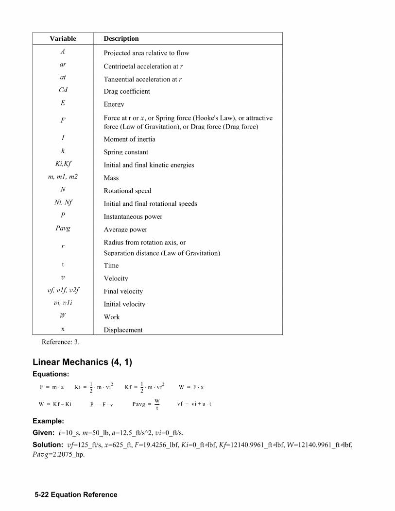
5-22 Equation Reference
Variable Description
A Projected area relative to flowar Centripetal acceleration at rat Tangential acceleration at rCd Drag coefficient E Energy
F Force at r or x, or Spring force (Hooke's Law), or attractive force (Law of Gravitation), or Drag force (Drag force)
I Moment of inertia k Spring constant
Ki,Kf Initial and final kinetic energiesm, m1, m2 Mass
N Rotational speed Ni, Nf Initial and final rotational speeds
P Instantaneous powerPavg Average power
r Radius from rotation axis, or Separation distance (Law of Gravitation)
t Timev Velocity
vf, v1f, v2f Final velocity vi, v1i Initial velocity
W Work x Displacement
Reference: 3. Linear Mechanics (4, 1) Equations:
F m a⋅= Ki 12--- m vi2⋅ ⋅= Kf 1
2--- m vf2⋅ ⋅=
W Kf Ki= vf vi a+ t⋅=P F v⋅= Pavg Wt
-----=
W F x⋅=
Example: Given: t=10_s, m=50_lb, a=12.5_ft/s^2, vi=0_ft/s.
Solution: vf=125_ft/s, x=625_ft, F=19.4256_lbf, Ki=0_ft∗lbf, Kf=12140.9961_ft∗lbf, W=12140.9961_ft∗lbf, Pavg=2.2075_hp.
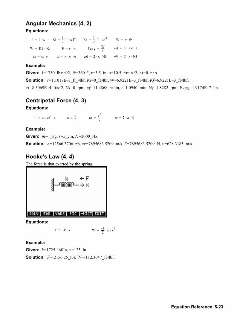
Equation Reference 5-23
Angular Mechanics (4, 2) Equations:
Example: Given: I=1750_lb∗in^2, Θ =360_°, r=3.5_in, α=10.5_r/min^2, ωi=0_r / s.
Solution: r=1.1017E3_ft_∗lbf, Ki=0_ft∗lbf, W=6.9221E3_ft∗lbf, Kf=6.9221E3_ft∗lbf,
at=8.5069E4_ft/s^2, Ni=0_rpm, ωf=11.4868_r/min, t=1.0940_min, Nf=1.8282_rpm, Pavg=1.9174E7_hp.
Centripetal Force (4, 3) Equations:
Example: Given: m=1_kg, r=5_cm, N=2000_Hz.
Solution: ω=12566.3706_r/s, ar=7895683.5209_m/s, F=7895683.5209_N, v=628.3185_m/s.
Hooke's Law (4, 4) The force is that exerted by the spring.
Equations:
F k x⋅= W 12
------ k x2⋅ ⋅=
Example: Given: k=1725_lbf/in, x=125_in.
Solution: F=-2156.25_lbf, W=-112.3047_ft∗lbf.
τ I α ⋅ = K i 1 2 - - - I ω i 2 ⋅ ⋅ = K f 1
2 - - - I ω f2⋅ ⋅=
W K f K i = ω f ω i α+ t⋅=P τ ω ⋅ = P a v g Wt
-----=
W r Θ⋅=
a t α r ⋅ = ω f 2 π Nf⋅ ⋅=ω 2 π N ⋅ ⋅ = ω i 2 π Ni⋅ ⋅=
F m ω 2 r ⋅ ⋅ = ω 2 π N⋅ ⋅=ω v r - - - = a r v2
r-----=
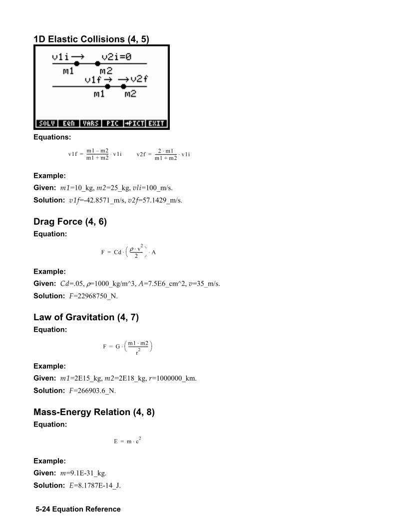
5-24 Equation Reference
1D Elastic Collisions (4, 5)
Equations:
v1f m1 m2m1 m2+---------------------- v1i⋅= v2f 2 m1⋅
m1 m2+---------------------- v1i⋅=
Example: Given: m1=10_kg, m2=25_kg, vli=100_m/s.
Solution: v1f=-42.8571_m/s, v2f=57.1429_m/s.
Drag Force (4, 6) Equation:
Example: Given: Cd=.05, ρ=1000_kg/m^3, A=7.5E6_cm^2, v=35_m/s.
Solution: F=22968750_N. Law of Gravitation (4, 7) Equation:
F G m1 m2⋅
r2--------------------⎝ ⎠
⎛ ⎞⋅=
Example: Given: m1=2E15_kg, m2=2E18_kg, r=1000000_km.
Solution: F=266903.6_N.
Mass-Energy Relation (4, 8) Equation:
E m c2⋅=
Example: Given: m=9.1E-31_kg.
Solution: E=8.1787E-14_J.
F C d ρ v 2 ⋅ 2 - - - - - - - - - - - - - ⎝ ⎠
⎛ ⎞ A ⋅ ⋅ =
Equation Reference 5-25
Gases (5)
Variable Description
λ Mean free path ρ Flow density
ρ0 Stagnation densityA Flow area At Throat area d Molecular diameterk Specific heat ratioM Mach number m Mass
MW Molecular weight
n Number of moles, or Polytropic constant (Polytropic Processes)
P Pressure, or Flow pressure (Isentropic Flow)P0 Stagnation pressurePc Pseudocritical pressure
Pi, Pf Initial and final pressuresT Temperature, or Flow temperature (Isentropic Flow)
T0 Stagnation temperatureTc Pseudocritical temperature
Ti, Tf Initial and final temperatureV Volume
Vi, Vf Initial and final volumesvrms Root-mean-square (rms) velocity
W Work
References:1, 3. Ideal Gas Law (5, 1) Equations:
P V⋅ n R T⋅ ⋅= m n MW⋅=
5-26 Equation Reference
Example: Given: T=16.85_°C, P=1_atm, V=25_1, MW=36_g/gmol.
Solution: n=1.0506_gmol, m=3.7820E-2_kg.
Ideal Gas State Change (5, 2) Equation:
Pf Vf⋅Tf
---------------- Pi Vi⋅Ti
----------------=
Example: Given: Pi=1.5_kPa, Pf=1.5kPa, Vi=2_l, Ti=100_°C, Tf=373.15_K.
Solution: Vf=2_1.
Isothermal Expansion (5, 3) These equations apply to an ideal gas. Equations:
W n R T LN VfVi------⎝ ⎠
⎛ ⎞⋅ ⋅ ⋅= m n MW⋅=
Example: Given: Vi=2_l, Vf=125_l, T=300_°C, n=0.25_gmol, MW=64_g/gmol.
Solution: W=4926.4942_J, M=0.016_kg. Polytropic Processes (5, 4) These equations describe a reversible pressure-volume change of an ideal gas such that P ∗Vn is constant. Special cases include isothermal processes (n=1), isentropic processes (n=k, the specific heat ratio), and constant-pressure processes (n=0). Equations:
PfPi----- Vf
Vi------⎝ ⎠
⎛ ⎞ n= Tf
Ti------ Pf
Pi-----⎝ ⎠
⎛ ⎞n 1
n------------
=
Example: Given: Pi=15_psi, Pf=35_psi, Vi=1_ft^3, Vf=0.50_ft^3, Ti=75_°F.
Solution: n=1.2224, Tf=164.1117_°F. Isentropic Flow (5, 5) The calculation differs at velocities below and above Mach 1. The Mach number is based on the speed of sound in the compressible fluid.
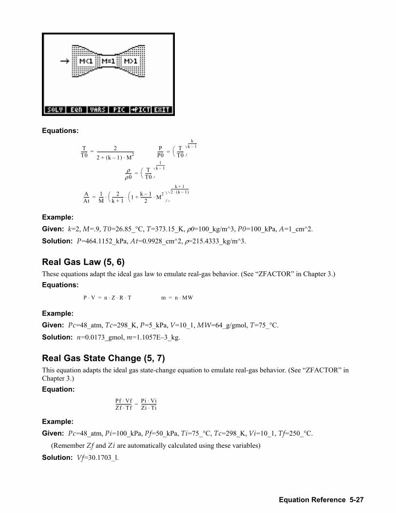
Equation Reference 5-27
Equations:
T T 0 - - - - - - - 2
2 k 1 ( ) + M 2 ⋅ - - - - - - - - - - - - - - - - - - - - - -- - - - - - - - - - - - - - - - = P
P0- ----- T
T0-------⎝ ⎠
⎛ ⎞k
k 1------------
=
ρ ρ 0 - - - - - - - T
T 0 - - - - - - - ⎝ ⎠ ⎛ ⎞ 1
k 1- - - ---------
=
A A t - - - - - - 1
M - - - - - 2k 1 + - - - - - - - - - - - - 1 k 1
2 - - - - - - - - - - - - + M2⋅ ⎝ ⎠⎛ ⎞⋅ ⎝ ⎠
⎛ ⎞k 1+
2 k 1( )⋅------------------------
⋅ =
Example: Given: k=2, M=.9, T0=26.85_°C, T=373.15_K, ρ0=100_kg/m^3, P0=100_kPa, A=1_cm^2.
Solution: P=464.1152_kPa, At=0.9928_cm^2, ρ=215.4333_kg/m^3.
Real Gas Law (5, 6) These equations adapt the ideal gas law to emulate real-gas behavior. (See ZFACTOR in Chapter 3.) Equations:
P V⋅ n Z R T⋅ ⋅ ⋅= m n MW⋅=
Example: Given: Pc=48_atm, Tc=298_K, P=5_kPa, V=10_1, MW=64_g/gmol, T=75_°C.
Solution: n=0.0173_gmol, m=1.1057E3_kg.
Real Gas State Change (5, 7) This equation adapts the ideal gas state-change equation to emulate real-gas behavior. (See ZFACTOR in Chapter 3.) Equation:
Pf Vf⋅Zf Tf⋅---------------- Pi Vi⋅
Zi Ti⋅----------------=
Example: Given: Pc=48_atm, Pi=100_kPa, Pf=50_kPa, Ti=75_°C, Tc=298_K, Vi=10_1, Tf=250_°C.
(Remember Zf and Zi are automatically calculated using these variables)
Solution: Vf=30.1703_l.
5-28 Equation Reference
Kinetic Theory (5, 8) These equations describe properties of an ideal gas. Equations:
P n MW vrms2⋅ ⋅3 V⋅
---------------------------------------= vrms 3 R T⋅ ⋅MW
-------------------=
λ 1
2 π n NA⋅V
----------------⎝ ⎠⎛ ⎞ d2⋅ ⋅ ⋅
---------------------------------------------------= m n MW⋅=
Example: Given: P=100_kPa, V=2_1, T=26.85_°C, MW=18_g/gmol, d=2.5_nm.
Solution: vrms=644.7678_m/s, m=1.4433E3_kg, n=0.0802_gmol, λ=1.4916_nm.
Heat Transfer (6) Variable Description
α Expansion coefficient δ Elongation
λ1, λ2 Lower and upper wavelength limits λmax Wavelength of maximum emissive power ∆T Temperature difference A Area c Specific heat
eb12 Emissive power in the range λ1 to λ2 eb Total emissive power f Fraction of emissive power in the range λ1 to λ2
h, h1,h3 Convective heat-transfer coefficient k, k1, k2, k3 Thermal conductivity L, L1, L2, L3 Length
m Mass Q Heat capacity q Heat transfer rate T Temperature
Tc Cold surface temperature (Conduction), or Cold fluid temperature
Th Hot surface temperature, or Hot fluid temperature (Conduction + Convection)
Ti, Tf Initial and final temperature U Overall heat transfer coefficient
References: 7, 9.
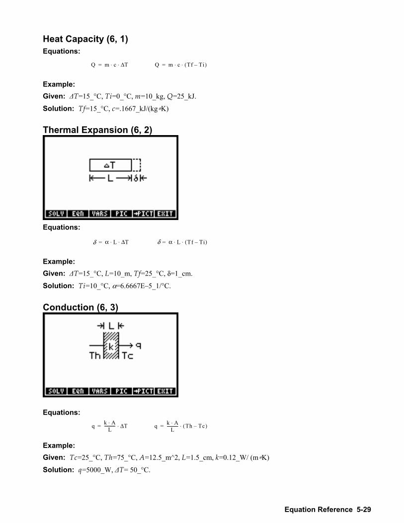
Equation Reference 5-29
Heat Capacity (6, 1) Equations:
Q m c T∆⋅ ⋅= Q m c Tf Ti( )⋅ ⋅=
Example: Given: ∆T=15_°C, Ti=0_°C, m=10_kg, Q=25_kJ.
Solution: Tf=15_°C, c=.1667_kJ/(kg∗K)
Thermal Expansion (6, 2)
Equations:
Example: Given: ∆T=15_°C, L=10_m, Tf=25_°C, δ=1_cm.
Solution: Ti=10_°C, α=6.6667E5_1/°C. Conduction (6, 3)
Equations:
q k A⋅L
----------- T∆⋅= q k A⋅L
----------- Th Tc( )⋅=
Example: Given: Tc=25_°C, Th=75_°C, A=12.5_m^2, L=1.5_cm, k=0.12_W/ (m∗K)
Solution: q=5000_W, ∆T= 50_°C.
δ α L T ∆ ⋅ ⋅ = δ α L Tf Ti( )⋅ ⋅=
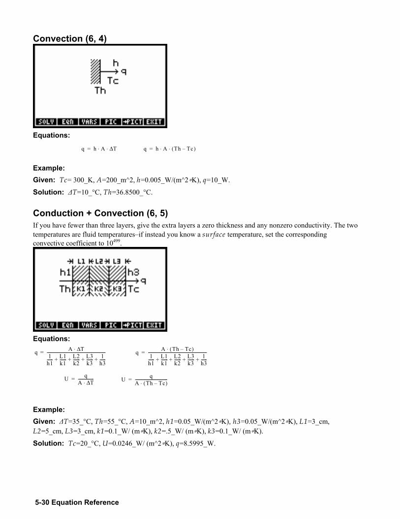
5-30 Equation Reference
Convection (6, 4)
Equations:
q h A T∆⋅ ⋅= q h A Th Tc( )⋅ ⋅=
Example: Given: Tc= 300_K, A=200_m^2, h=0.005_W/(m^2∗K), q=10_W.
Solution: ∆T=10_°C, Th=36.8500_°C. Conduction + Convection (6, 5) If you have fewer than three layers, give the extra layers a zero thickness and any nonzero conductivity. The two temperatures are fluid temperaturesif instead you know a surface temperature, set the corresponding convective coefficient to 10499.
Equations:
q A T∆⋅1
h1------ L1
k1------- L2
k2------- L3
k3------- 1
h3------+ + + +
------------------------------------------------------------= q A Th Tc( )⋅1
h1------ L1
k1------- L2
k2------- L3
k3------- 1
h3------+ + + +
------------------------------------------------------------=
U qA T∆⋅----------------= U q
A Th Tc( )⋅---------------------------------=
Example: Given: ∆T=35_°C, Th=55_°C, A=10_m^2, h1=0.05_W/(m^2∗K), h3=0.05_W/(m^2∗K), L1=3_cm, L2=5_cm, L3=3_cm, k1=0.1_W/ (m∗K), k2=.5_W/ (m∗K), k3=0.1_W/ (m∗K).
Solution: Tc=20_°C, U=0.0246_W/ (m^2∗K), q=8.5995_W.
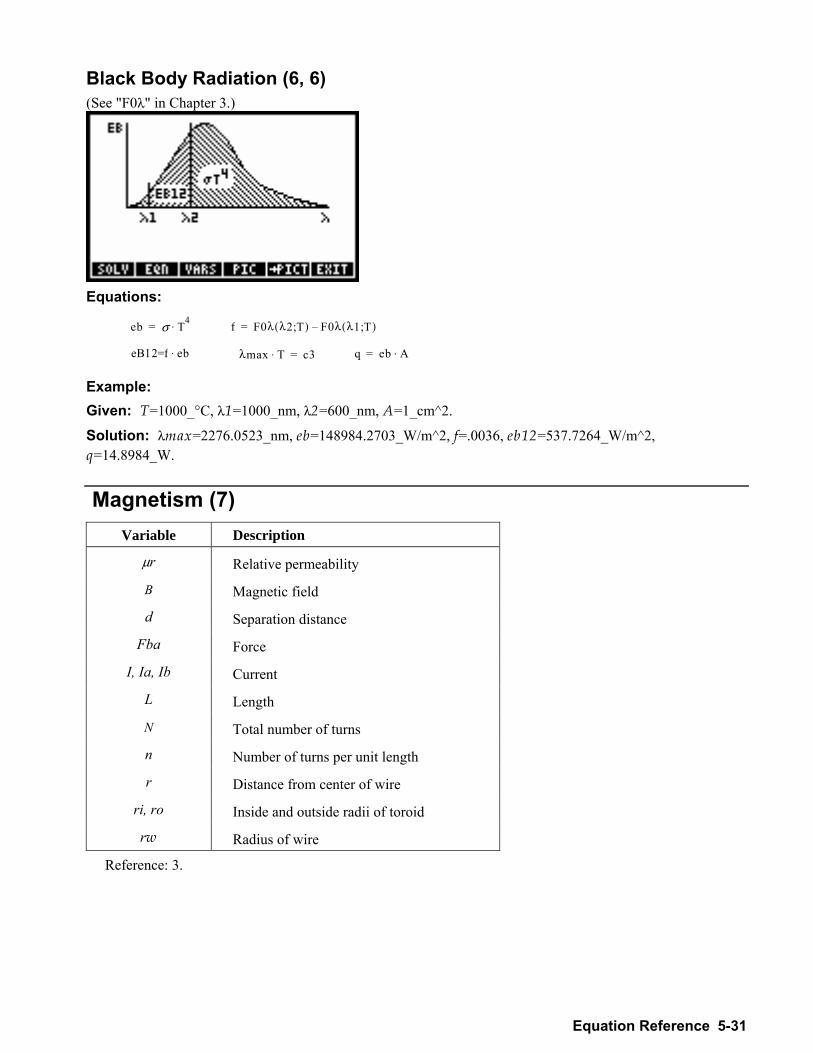
Equation Reference 5-31
Black Body Radiation (6, 6) (See "F0λ" in Chapter 3.)
Equations:
Example: Given: T=1000_°C, λ1=1000_nm, λ2=600_nm, A=1_cm^2.
Solution: λmax=2276.0523_nm, eb=148984.2703_W/m^2, f=.0036, eb12=537.7264_W/m^2, q=14.8984_W.
Magnetism (7) Variable Description
µr Relative permeability
B Magnetic field
d Separation distance
Fba Force
I, Ia, Ib Current
L Length
N Total number of turns
n Number of turns per unit length
r Distance from center of wire
ri, ro Inside and outside radii of toroid
rw Radius of wire
Reference: 3.
e b σ T 4 ⋅ = f F 0 λ λ 2 T ; ( ) F0λ λ1 T;( ) =
eB1 f e b ⋅ 2= λ m ax T ⋅ c 3 = q eb A⋅=
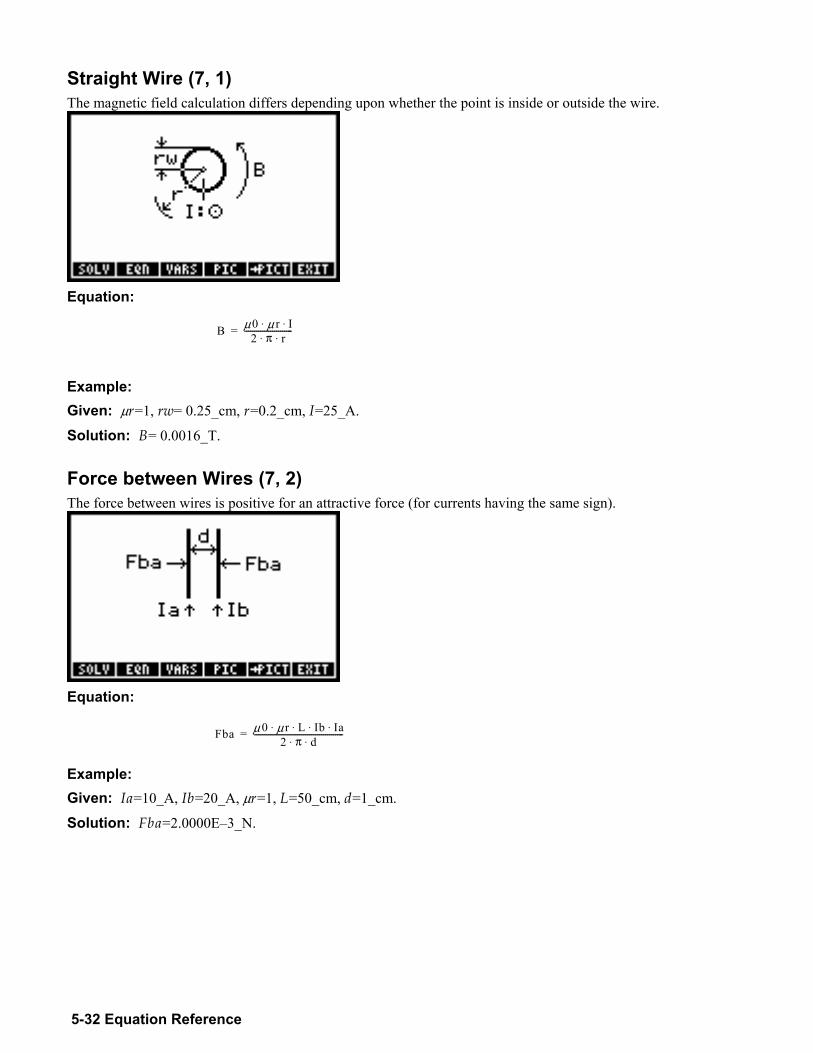
5-32 Equation Reference
Straight Wire (7, 1) The magnetic field calculation differs depending upon whether the point is inside or outside the wire.
Equation:
Example: Given: µr=1, rw= 0.25_cm, r=0.2_cm, I=25_A.
Solution: B= 0.0016_T.
Force between Wires (7, 2) The force between wires is positive for an attractive force (for currents having the same sign).
Equation:
Example: Given: Ia=10_A, Ib=20_A, µr=1, L=50_cm, d=1_cm.
Solution: Fba=2.0000E3_N.
B µ 0 µ r I ⋅ ⋅ 2 π r ⋅ ⋅ - - - - - - - - - - - - - - - - - - - - - - - - =
F b a µ 0 µ r L I b Ia⋅ ⋅ ⋅ ⋅2 π d ⋅ ⋅ - - - - - - - - - - - - - - - - - - - - - - - - - - - - - - - - - - - - ---------=
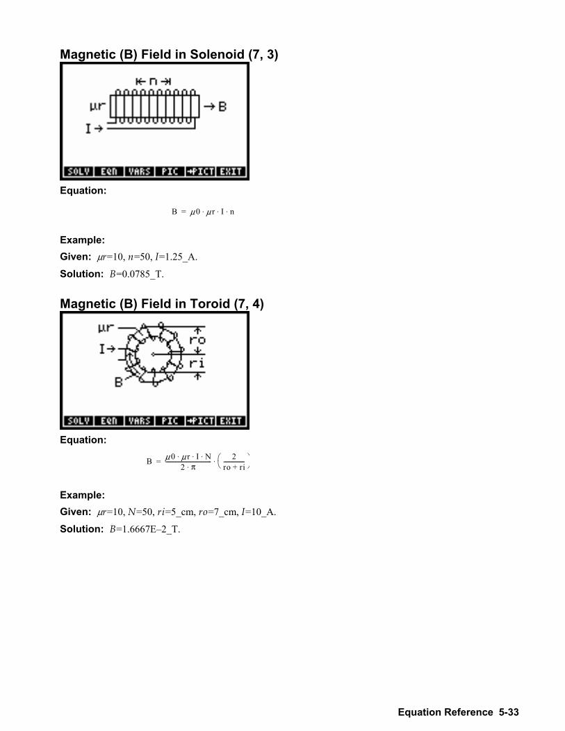
Equation Reference 5-33
Magnetic (B) Field in Solenoid (7, 3)
Equation:
Example: Given: µr=10, n=50, I=1.25_A.
Solution: B=0.0785_T.
Magnetic (B) Field in Toroid (7, 4)
Equation:
Example: Given: µr=10, N=50, ri=5_cm, ro=7_cm, I=10_A.
Solution: B=1.6667E2_T.
B µ 0 µ r I n⋅ ⋅ ⋅=
B µ0 µ r I N ⋅ ⋅ ⋅ 2 π ⋅ - -- - - - - - - - - - - - - - - - - - - - - - - - - - - - - - - 2
r o ri+- --------------⎝ ⎠
⎛ ⎞⋅ =
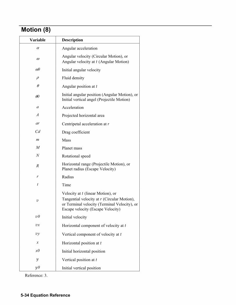
5-34 Equation Reference
Motion (8) Variable Description
α Angular acceleration
ω Angular velocity (Circular Motion), or Angular velocity at t (Angular Motion)
ω0 Initial angular velocity
ρ Fluid density
θ Angular position at t
θ0 Initial angular position (Angular Motion), or Initial vertical angel (Projectile Motion)
a Acceleration
A Projected horizontal area
ar Centripetal acceleration at r
Cd Drag coefficient
m Mass
M Planet mass
N Rotational speed
R Horizontal range (Projectile Motion), or Planet radius (Escape Velocity)
r Radius
t Time
v Velocity at t (linear Motion), or Tangential velocity at r (Circular Motion), or Terminal velocity (Terminal Velocity), or Escape velocity (Escape Velocity)
v0 Initial velocity
vx Horizontal component of velocity at t
vy Vertical component of velocity at t
x Horizontal position at t
x0 Initial horizontal position
y Vertical position at t
y0 Initial vertical position
Reference: 3.
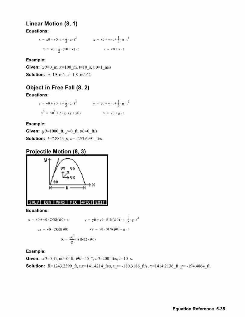
Equation Reference 5-35
Linear Motion (8, 1) Equations:
x x0 v0+ t⋅ 12---+ a t2⋅ ⋅= x x0 v+ t⋅ 1
2---+ a t2⋅ ⋅=
x x0 12---+ v0 v+( ) t⋅ ⋅= v v0 a+ t⋅=
Example: Given: x0=0_m, x=100_m, t=10_s, v0=1_m/s
Solution: v=19_m/s, a=1.8_m/s^2.
Object in Free Fall (8, 2) Equations:
y y0 v0+ t⋅ 12---+ g t2⋅ ⋅= y y0 v+ t⋅ 1
2---+ g t2⋅ ⋅=
v2 v02 2 g⋅+ y y0+( )⋅= v v0 g+ t⋅=
Example: Given: y0=1000_ft, y=0_ft, v0=0_ft/s
Solution: t=7.8843_s, v= -253.6991_ft/s.
Projectile Motion (8, 3)
Equations:
Example: Given: x0=0_ft, y0=0_ft, Θ 0 =45_°, v0=200_ft/s, t=10_s.
Solution: R=1243.2399_ft, vx=141.4214_ft/s, vy= -180.3186_ft/s, x=1414.2136_ft, y= -194.4864_ft.
x x 0 v 0 + C O S ⋅ θ 0 ( ) t ⋅ = y y0 v0+ SIN θ 0( ) t⋅ ⋅ 12--- g t2⋅ ⋅=
v x v 0 C O S θ 0 ( ) ⋅ = v y v0 SIN θ 0( ) g t⋅⋅=
R v 0 2 g - - - - - -- - S I N 2 θ 0 ⋅ ( ) ⋅ =
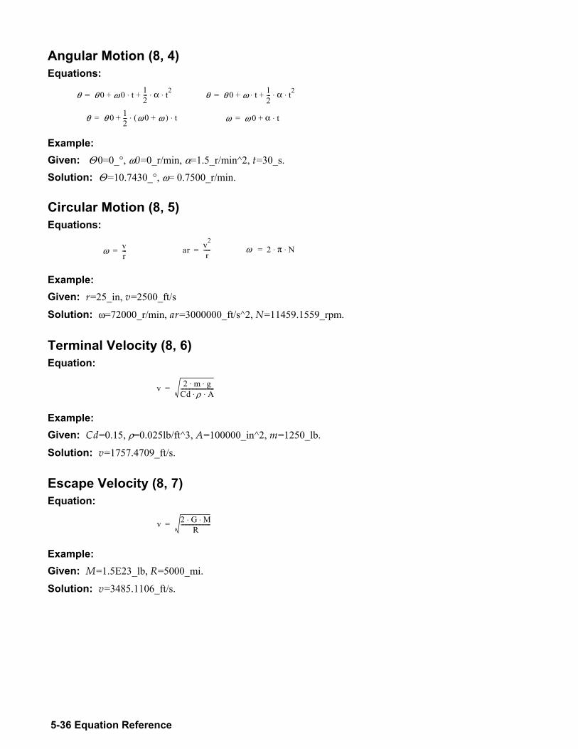
5-36 Equation Reference
Angular Motion (8, 4) Equations:
Example: Given: Θ 0=0_°, ω0=0_r/min, α=1.5_r/min^2, t=30_s.
Solution: Θ =10.7430_°, ω= 0.7500_r/min.
Circular Motion (8, 5) Equations:
Example: Given: r=25_in, v=2500_ft/s
Solution: ω=72000_r/min, ar=3000000_ft/s^2, N=11459.1559_rpm. Terminal Velocity (8, 6) Equation:
Example: Given: Cd=0.15, ρ=0.025lb/ft^3, A=100000_in^2, m=1250_lb.
Solution: v=1757.4709_ft/s.
Escape Velocity (8, 7) Equation:
v 2 G M⋅ ⋅R
---------------------=
Example: Given: M=1.5E23_lb, R=5000_mi.
Solution: v=3485.1106_ft/s.
θ θ 0 ω 0 + t ⋅ 1 2 - - - + α t 2 ⋅ ⋅ = θ θ 0 ω+ t⋅ 1
2---+ α t2⋅ ⋅=
θ θ 0 1 2 - - - + ω 0 ω + ( ) t ⋅ ⋅ = ω ω 0 α+ t⋅=
ω v r - - - = ar v 2
r - - - - - = ω 2 π N⋅ ⋅=
v 2 m g ⋅ ⋅ C d ρ ⋅ A ⋅ - - - - - - - - - - - - - - - - - - - - - - - - =
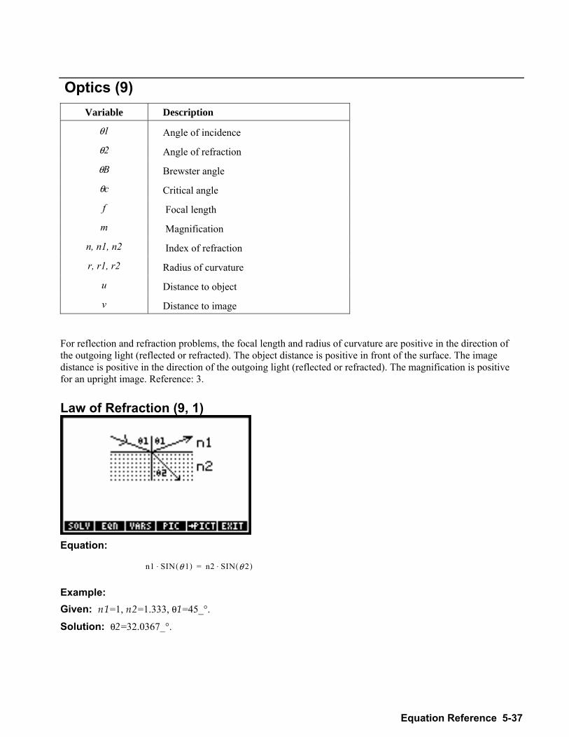
Equation Reference 5-37
Optics (9) Variable Description
θ1 Angle of incidence
θ2 Angle of refraction
θB Brewster angle
θc Critical angle
f Focal length
m Magnification
n, n1, n2 Index of refraction
r, r1, r2 Radius of curvature
u Distance to object
v Distance to image
For reflection and refraction problems, the focal length and radius of curvature are positive in the direction of the outgoing light (reflected or refracted). The object distance is positive in front of the surface. The image distance is positive in the direction of the outgoing light (reflected or refracted). The magnification is positive for an upright image. Reference: 3. Law of Refraction (9, 1)
Equation:
Example: Given: n1=1, n2=1.333, θ1=45_°.
Solution: θ2=32.0367_°.
n 1 S I N θ 1 ( ) ⋅ n 2 S I N θ 2( )⋅ =

5-38 Equation Reference
Critical Angle (9, 2)
Equation:
Example: Given: n1=1, n2=1.5.
Solution: θc=41.8103_°. Brewster's Law (9, 3) The Brewster angle is the angle of incidence at which the reflected wave is completely polarized.
Equations:
Example: Given: n1=1, n2=1.5.
Solution: θ B=56.3099_°, θ 2=33.6901_°.
S I N θ c ( ) n 1 n 2 - - - - - - =
T A N θ B ( ) n 2 n 1 - - - - - - = θ B θ 2+ 90=
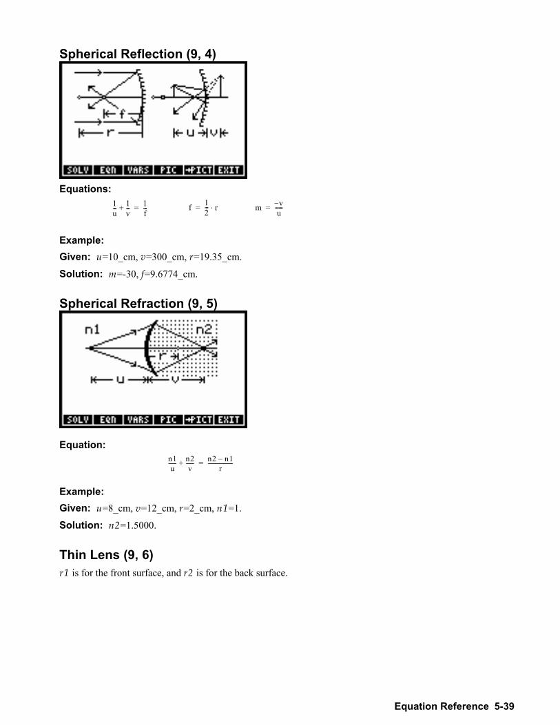
Equation Reference 5-39
Spherical Reflection (9, 4)
Equations:
1u--- 1
v---+ 1
f---= f 1
2--- r⋅= m v
u------=
Example: Given: u=10_cm, v=300_cm, r=19.35_cm.
Solution: m=-30, f=9.6774_cm.
Spherical Refraction (9, 5)
Equation: n1u
------ n2v
------+ n2 n1r
------------------=
Example: Given: u=8_cm, v=12_cm, r=2_cm, n1=1.
Solution: n2=1.5000.
Thin Lens (9, 6) r1 is for the front surface, and r2 is for the back surface.
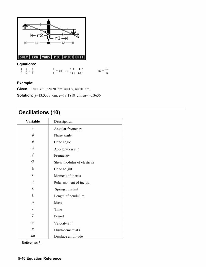
5-40 Equation Reference
Equations:
1u--- 1
v---+ 1
f---= 1
f--- n 1( ) 1
r1----- 1
r2-----⎝ ⎠
⎛ ⎞⋅= m vu
------=
Example: Given: r1=5_cm, r2=20_cm, n=1.5, u=50_cm.
Solution: f=13.3333_cm, v=18.1818_cm, m= -0.3636.
Oscillations (10) Variable Description
ω Angular frequency φ Phase angle
θ Cone angle a Acceleration at t f Frequency
G Shear modulus of elasticityh Cone height I Moment of inertia J Polar moment of inertiak Spring constant L Length of pendulumm Masst TimeT Period v Velocity at t x Displacement at t
xm Displace amplitude
Reference: 3.
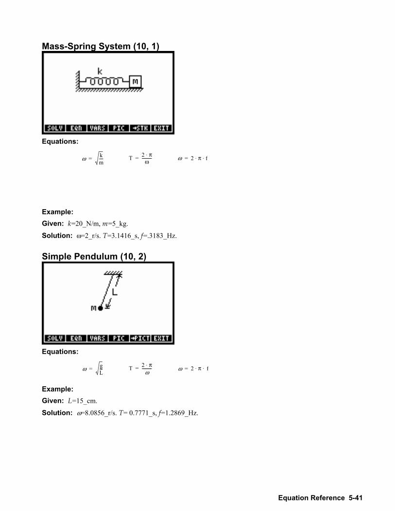
Equation Reference 5-41
Mass-Spring System (10, 1)
Equations:
Example: Given: k=20_N/m, m=5_kg.
Solution: ω=2_r/s. T=3.1416_s, f=.3183_Hz.
Simple Pendulum (10, 2)
Equations:
Example: Given: L=15_cm.
Solution: ω=8.0856_r/s. T= 0.7771_s, f=1.2869_Hz.
ω k m - - - - = T 2 π ⋅
ω - - - - - - - - - - = ω 2 π f⋅ ⋅=
ω g L - - - = T 2 π ⋅
ω - - - - - - - - - - = ω 2 π f⋅ ⋅=
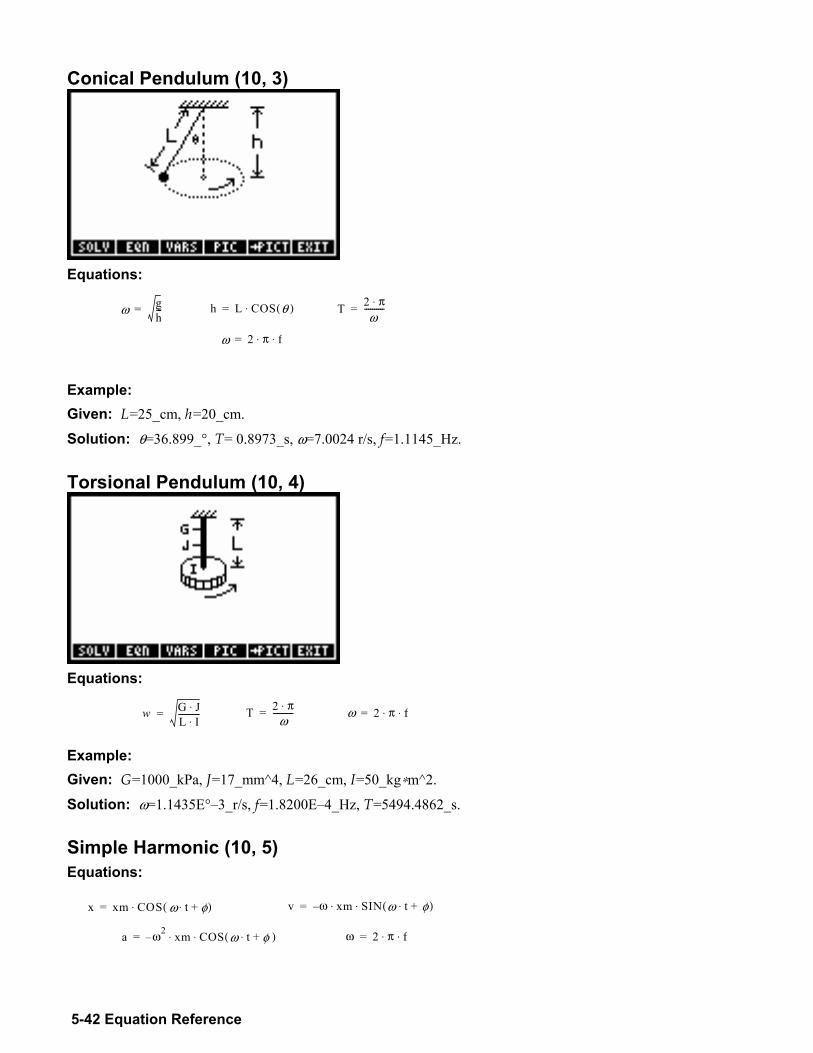
5-42 Equation Reference
Conical Pendulum (10, 3)
Equations:
Example: Given: L=25_cm, h=20_cm.
Solution: θ=36.899_°, T= 0.8973_s, ω=7.0024 r/s, f=1.1145_Hz. Torsional Pendulum (10, 4)
Equations:
Example: Given: G=1000_kPa, J=17_mm^4, L=26_cm, I=50_kg∗m^2.
Solution: ω=1.1435E°3_r/s, f=1.8200E4_Hz, T=5494.4862_s.
Simple Harmonic (10, 5) Equations:
ω g h - - - = h L C O S θ ( ) ⋅ = T 2 π⋅
ω----------=
ω 2 π f ⋅ ⋅ =
w G J ⋅ L I ⋅ - - - - - - - - - - - = T 2 π ⋅
ω - - - - - - - - - - = ω 2 π f⋅ ⋅=
x x m C O S ω t ⋅ φ + ( ) ⋅ = v ω xm SIN ω t⋅ φ+( )⋅ ⋅=
a ω 2 x m C O S ω t ⋅ φ + ( ) ⋅ ⋅ = ω 2 π f⋅ ⋅=
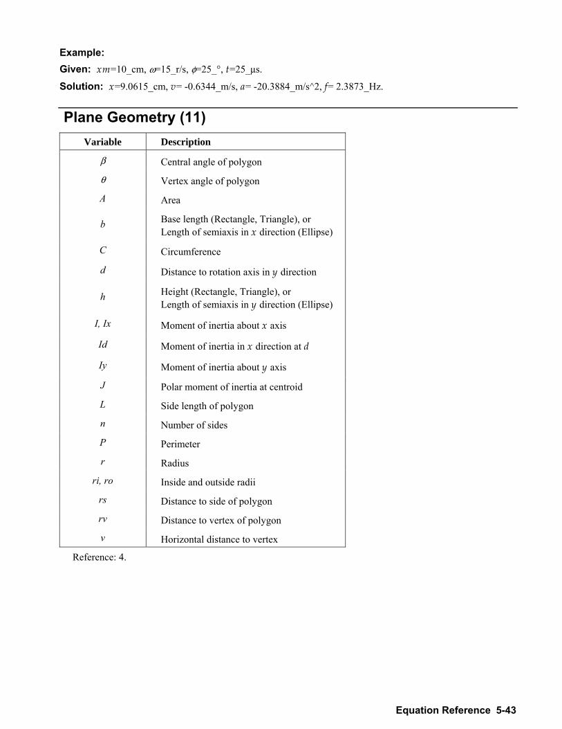
Equation Reference 5-43
Example: Given: xm=10_cm, ω=15_r/s, φ=25_°, t=25_µs.
Solution: x=9.0615_cm, v= -0.6344_m/s, a= -20.3884_m/s^2, f= 2.3873_Hz.
Plane Geometry (11) Variable Description
β Central angle of polygon
θ Vertex angle of polygon
A Area
b Base length (Rectangle, Triangle), or Length of semiaxis in x direction (Ellipse)
C Circumference
d Distance to rotation axis in y direction
h Height (Rectangle, Triangle), or Length of semiaxis in y direction (Ellipse)
I, Ix Moment of inertia about x axis
Id Moment of inertia in x direction at d
Iy Moment of inertia about y axis
J Polar moment of inertia at centroid
L Side length of polygon
n Number of sides
P Perimeter
r Radius
ri, ro Inside and outside radii
rs Distance to side of polygon
rv Distance to vertex of polygon
v Horizontal distance to vertex
Reference: 4.
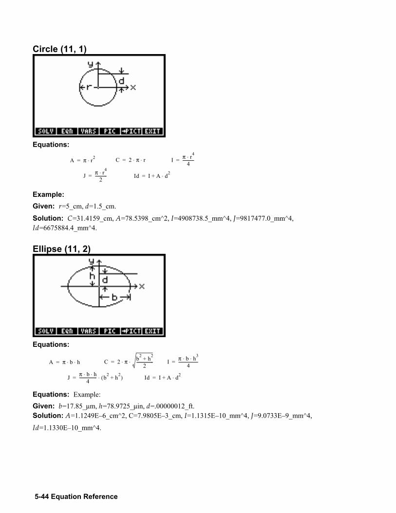
5-44 Equation Reference
Circle (11, 1)
Equations:
A π r2⋅= C 2 π r⋅ ⋅= I π r4⋅4
------------=
J π r4⋅2
------------= Id I A+ d2⋅=
Example: Given: r=5_cm, d=1.5_cm.
Solution: C=31.4159_cm, A=78.5398_cm^2, I=4908738.5_mm^4, J=9817477.0_mm^4, Id=6675884.4_mm^4. Ellipse (11, 2)
Equations:
A π b h⋅ ⋅= C 2 π b2 h2+2
-----------------⋅ ⋅= I π b h3⋅ ⋅4
--------------------=
J π b h⋅ ⋅4
------------------ b2 h2+( )⋅= Id I A+ d2⋅=
Equations: Example: Given: b=17.85_µm, h=78.9725_µin, d=.00000012_ft. Solution: A=1.1249E6_cm^2, C=7.9805E3_cm, I=1.1315E10_mm^4, J=9.0733E9_mm^4,
Id=1.1330E10_mm^4.
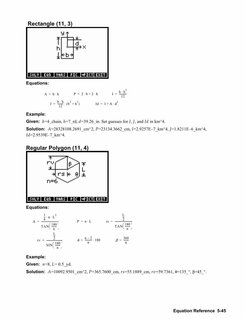
Equation Reference 5-45
Rectangle (11, 3)
Equations:
A b h⋅= P 2 b⋅ 2+ h⋅= I b h3⋅12
-------------=
J b h⋅12
---------- b2 h2+( )⋅= Id I A+ d2⋅=
Example: Given: b=4_chain, h=7_rd, d=39.26_in. Set guesses for I, J, and Id in km^4.
Solution: A=28328108.2691_cm^2, P=23134.3662_cm, I=2.9257E7_km^4, J=1.8211E6_km^4, Id=2.9539E7_km^4.
Regular Polygon (11, 4)
Equations:
A
1 4 - - - n L 2 ⋅ ⋅
T A N 180 n - - - - - - - - - ⎝ ⎠ ⎛ ⎞
- - - - - - - - - - - - - - - - - - - - - - - - - - - - - = P n L ⋅ = rs
L2---
TAN 180n
---------⎝ ⎠⎛ ⎞
-----------------------------=
r v L 2 - - -
S I N 180 n - - - - - - - - - ⎝ ⎠ ⎛ ⎞
- - - - - - - - - - - - - - - - - - - - - - - - - - - = θ n 2 n - - - - - - - - - - - - 180⋅ = β 360
n---------=
Example: Given: n=8, L= 0.5_yd.
Solution: A=10092.9501_cm^2, P=365.7600_cm, rs=55.1889_cm, rv=59.7361, θ=135_°, β=45_°.
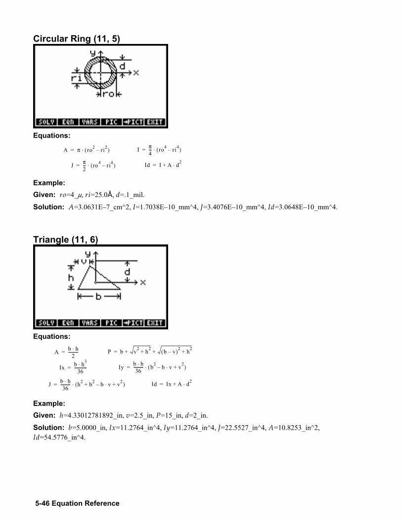
5-46 Equation Reference
Circular Ring (11, 5)
Equations:
A π ro2 ri2( )⋅= I π4--- ro4 ri4( )⋅=
J π2--- ro4 ri4( )⋅= Id I A d2⋅+=
Example: Given: ro=4_µ, ri=25.0Å, d=.1_mil.
Solution: A=3.0631E7_cm^2, I=1.7038E10_mm^4, J=3.4076E10_mm^4, Id=3.0648E10_mm^4. Triangle (11, 6)
Equations:
A b h⋅2
----------= P b v2 h2+ b v( )2 h2++ +=
Ix b h3⋅36
-------------= Iy b h⋅36
---------- b2 b v⋅ v2+( )⋅=
J b h⋅36
---------- h2 b2 b v⋅ v2+ +( )⋅= Id Ix A d2⋅+=
Example: Given: h=4.33012781892_in, v=2.5_in, P=15_in, d=2_in.
Solution: b=5.0000_in, Ix=11.2764_in^4, Iy=11.2764_in^4, J=22.5527_in^4, A=10.8253_in^2, Id=54.5776_in^4.
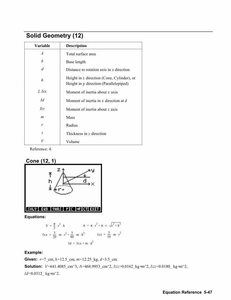
Equation Reference 5-47
Solid Geometry (12) Variable Description
A Total surface area
b Base length
d Distance to rotation axis in z direction
h Height in z direction (Cone, Cylinder), or Height in y direction (Parallelepiped)
I, Ixx Moment of inertia about x axis
Id Moment of inertia in x direction at d
Izz Moment of inertia about z axis
m Mass
r Radius
t Thickness in z direction
V Volume
Reference: 4.
Cone (12, 1)
Equations:
V π3--- r2 h⋅ ⋅= A π r2⋅ π r r2 h2+⋅ ⋅+=
Ixx 320------ m r2⋅ ⋅ 3
80------ m h2⋅ ⋅+= Izz 3
10------ m r2⋅ ⋅=
Id Ixx m d2⋅+=
Example: Given: r=7_cm, h=12.5_cm, m=12.25_kg, d=3.5_cm.
Solution: V=641.4085_cm^3, A=468.9953_cm^2, Izz=0.0162_kg∗m^2, Izz=0.0180_ kg∗m^2,
Id=0.0312_ kg∗m^2.
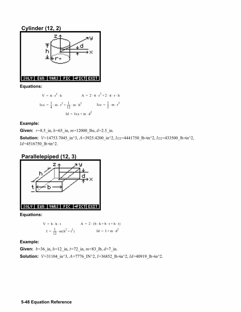
5-48 Equation Reference
Cylinder (12, 2)
Equations:
V π r2 h⋅ ⋅= A 2 π r2⋅ ⋅ 2 π r h⋅ ⋅ ⋅+=
Ixx 14--- m r2⋅ ⋅ 1
12------ m h2⋅ ⋅+= Izz 1
2--- m r2⋅ ⋅=
Id Ixx m d2⋅+=
Example: Given: r=8.5_in, h=65_in, m=12000_lbs, d=2.5_in.
Solution: V=14753.7045_in^3, A=3925.4200_in^2, Izz=4441750_lb∗in^2, Izz=433500_lb∗in^2, Id=4516750_lb∗in^2. Parallelepiped (12, 3)
Equations:
V b h t⋅ ⋅= A 2 b h⋅ b t⋅ h t⋅+ +( )⋅=
I 112------ m⋅ h2 t2+( )= Id I m d2⋅+=
Example: Given: b=36_in, h=12_in, t=72_in, m=83_lb, d=7_in.
Solution: V=31104_in^3, A=7776_IN^2, I=36852_lb∗in^2, Id=40919_lb∗in^2.
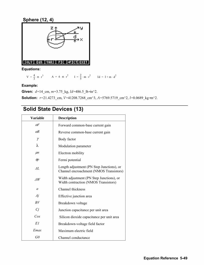
Equation Reference 5-49
Sphere (12, 4)
Equations:
V 43--- π r3⋅ ⋅= A 4 π r2⋅ ⋅= I 2
5--- m r2⋅ ⋅= Id I m d2⋅+=
Example: Given: d=14_cm, m=3.75_kg, Id=486.5_lb∗in^2.
Solution: r=21.4273_cm, V=41208.7268_cm^3, A=5769.5719_cm^2, I=0.0689_kg∗m^2.
Solid State Devices (13) Variable Description
αF Forward common-base current gain
αR Reverse common-base current gain
γ Body factor
λ Modulation parameter
µn Electron mobility
φp Fermi potential
∆L Length adjustment (PN Step Junctions), or Channel encroachment (NMOS Transistors)
∆W Width adjustment (PN Step Junctions), or Width contraction (NMOS Transistors)
a Channel thickness
Aj Effective junction area
BV Breakdown voltage
Cj Junction capacitance per unit area
Cox Silicon dioxide capacitance per unit area
E1 Breakdown-voltage field factor
Emax Maximum electric field
G0 Channel conductance
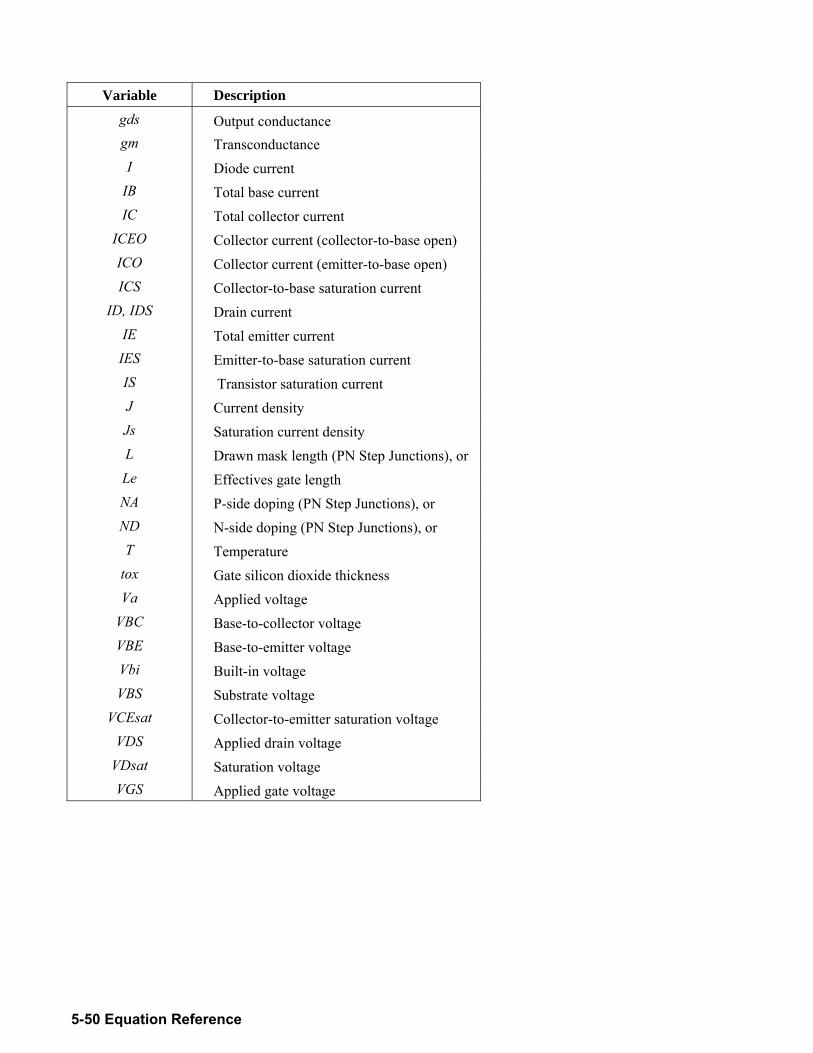
5-50 Equation Reference
Variable Description
gds Output conductance gm Transconductance I Diode current
IB Total base current IC Total collector current
ICEO Collector current (collector-to-base open) ICO Collector current (emitter-to-base open) ICS Collector-to-base saturation current
ID, IDS Drain current IE Total emitter current
IES Emitter-to-base saturation current IS Transistor saturation current J Current density Js Saturation current density L Drawn mask length (PN Step Junctions), or Le Effectives gate length NA P-side doping (PN Step Junctions), or ND N-side doping (PN Step Junctions), or T Temperature
tox Gate silicon dioxide thickness Va Applied voltage
VBC Base-to-collector voltage VBE Base-to-emitter voltage Vbi Built-in voltage VBS Substrate voltage
VCEsat Collector-to-emitter saturation voltage VDS Applied drain voltage
VDsat Saturation voltage VGS Applied gate voltage
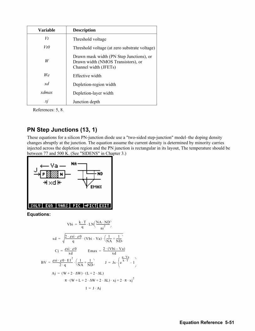
Equation Reference 5-51
Variable Description
Vt Threshold voltage
Vt0 Threshold voltage (at zero substrate voltage)
W Drawn mask width (PN Step Junctions), or Drawn width (NMOS Transistors), or Channel width (JFETs)
We Effective width
xd Depletion-region width
xdmax Depletion-layer width
xj Junction depth
References: 5, 8. PN Step Junctions (13, 1) These equations for a silicon PN-junction diode use a "two-sided step-junction" modelthe doping density changes abruptly at the junction. The equation assume the current density is determined by minority carries injected across the depletion region and the PN junction is rectangular in its layout, The temperature should be between 77 and 500 K. (See "SIDENS" in Chapter 3.)
Equations:
V b i k T ⋅ q - - - - - - - - - - - L N N A ND⋅
n i2- - - - - - - - - -------------⎝ ⎠⎛ ⎞⋅ =
x d 2 ε s i ε 0 ⋅ ⋅ q - - - - - - - - - - - - - - - - - -- - - - - - - - V b i V a ( ) 1
NA--------- 1
ND---------+⎝ ⎠
⎛ ⎞⋅ ⋅=
C j ε s i ε 0⋅ x d - - - - - - - - - - - - - - - - - - -= E m a x 2 Vbi Va( )⋅
xd-----------------------------------=
B V ε s i ε 0 E 1 2 ⋅ ⋅ 2 q ⋅ - - - - - - - - - - - - - - - - - - - - - - - - - - - - - - - - - 1
N A - - - - - - - - - 1 N D - - - - - - - - - + ⎝ ⎠ ⎛ ⎞ ⋅ = J Js e
q Va⋅k T⋅
--------------1
⎝ ⎠⎜⎛ ⎞
⋅=
π W L 2 W ∆ ⋅ 2 L∆⋅+ + + ( ) xj⋅ ⋅ 2+ π xj2⋅ ⋅
A j W 2 W ∆ ⋅ + ( ) L 2 L ∆ ⋅ + ( )⋅ =
I J A j ⋅ =
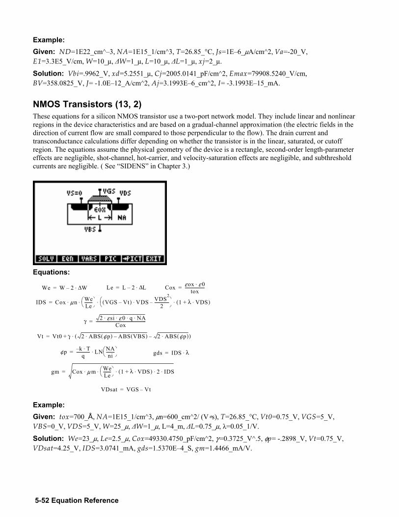
5-52 Equation Reference
Example: Given: ND=1E22_cm^3, NA=1E15_1/cm^3, T=26.85_°C, Js=1E6_µA/cm^2, Va=-20_V, E1=3.3E5_V/cm, W=10_µ, ∆W=1_µ, L=10_µ, ∆L=1_µ, xj=2_µ.
Solution: Vbi=.9962_V, xd=5.2551_µ, Cj=2005.0141_pF/cm^2, Emax=79908.5240_V/cm, BV=358.0825_V, J= -1.0E12_A/cm^2, Aj=3.1993E6_cm^2, I= -3.1993E15_mA.
NMOS Transistors (13, 2) These equations for a silicon NMOS transistor use a two-port network model. They include linear and nonlinear regions in the device characteristics and are based on a gradual-channel approximation (the electric fields in the direction of current flow are small compared to those perpendicular to the flow). The drain current and transconductance calculations differ depending on whether the transistor is in the linear, saturated, or cutoff region. The equations assume the physical geometry of the device is a rectangle, second-order length-parameter effects are negligible, shot-channel, hot-carrier, and velocity-saturation effects are negligible, and subthreshold currents are negligible. ( See SIDENS in Chapter 3.)
Equations:
W e W 2 W ∆ ⋅ =
I D S C o x µ n W e L e - - - - - - - - ⎝ ⎠ ⎛ ⎞ V G S V t ( ) V D S ⋅ V DS2
2- - - - - ---------- ⎝ ⎠
⎛ ⎞ 1 λ+ VDS⋅( )⋅ ⋅ ⋅ ⋅=
γ 2 ε s i ε 0 q N A ⋅ ⋅ ⋅ ⋅ C o x - - - - - - - - - - - - - - - - - - - - - - - -- - - - - - - - - - - - - - - - - - - - - - - - - - - =
V t V t 0 γ 2 A B S φ p ( ) ⋅ A B S V B S ( ) 2 ABS φp( )⋅ ( )⋅ + =
φ p k T ⋅ q - - - - - - - - - - - - - - L N N A
n i - - - - - - - - - ⎝ ⎠ ⎛ ⎞ ⋅ = g d s IDS λ⋅=
g m C o x µ m W e L e - - - - - - - - ⎝ ⎠ ⎛ ⎞ 1 λ + V D S ⋅ ( ) 2 IDS⋅ ⋅ ⋅ ⋅ ⋅=
V D s a t V G S V t =
L e L 2 L ∆ ⋅ = Cox εox ε 0⋅tox
--------------------=
Example: Given: tox=700_Å, NA=1E15_1/cm^3, µn=600_cm^2/ (V∗s), T=26.85_°C, Vt0=0.75_V, VGS=5_V, VBS=0_V, VDS=5_V, W=25_µ, ∆W=1_µ, L=4_m, ∆L=0.75_µ, λ=0.05_1/V.
Solution: We=23_µ, Le=2.5_µ, Cox=49330.4750_pF/cm^2, γ =0.3725_V^.5, φp= -.2898_V, Vt=0.75_V, VDsat=4.25_V, IDS=3.0741_mA, gds=1.5370E4_S, gm=1.4466_mA/V.
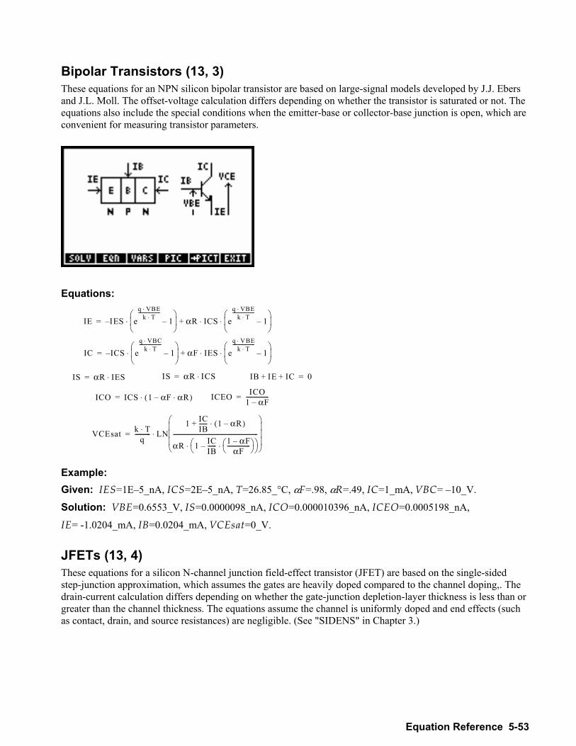
Equation Reference 5-53
Bipolar Transistors (13, 3) These equations for an NPN silicon bipolar transistor are based on large-signal models developed by J.J. Ebers and J.L. Moll. The offset-voltage calculation differs depending on whether the transistor is saturated or not. The equations also include the special conditions when the emitter-base or collector-base junction is open, which are convenient for measuring transistor parameters.
Equations:
IS αR IES⋅=
IE IES eq VBE⋅
k T⋅--------------------
1⎝ ⎠⎜ ⎟⎛ ⎞
⋅ αR ICS eq VBE⋅
k T⋅--------------------
1⎝ ⎠⎜ ⎟⎛ ⎞
⋅ ⋅+=
IS αR ICS⋅= IB IE IC+ + 0=
IC ICS eq VBC⋅
k T⋅--------------------
1⎝ ⎠⎜ ⎟⎛ ⎞
⋅ αF IES eq VBE⋅
k T⋅--------------------
1⎝ ⎠⎜ ⎟⎛ ⎞
⋅ ⋅+=
ICO ICS 1 αF αR⋅( )⋅= ICEO ICO1 αF----------------=
VCEsat k T⋅q
----------- LN1 IC
IB------ 1 αR( )⋅+
αR 1 ICIB------ 1 αF
αF----------------⎝ ⎠⎛ ⎞⋅⎝ ⎠
⎛ ⎞⋅------------------------------------------------------------
⎝ ⎠⎜ ⎟⎜ ⎟⎜ ⎟⎛ ⎞
⋅=
Example: Given: IES=1E5_nA, ICS=2E5_nA, T=26.85_°C, αF=.98, αR=.49, IC=1_mA, VBC= 10_V.
Solution: VBE=0.6553_V, IS=0.0000098_nA, ICO=0.000010396_nA, ICEO=0.0005198_nA,
IE= -1.0204_mA, IB=0.0204_mA, VCEsat=0_V.
JFETs (13, 4) These equations for a silicon N-channel junction field-effect transistor (JFET) are based on the single-sided step-junction approximation, which assumes the gates are heavily doped compared to the channel doping,. The drain-current calculation differs depending on whether the gate-junction depletion-layer thickness is less than or greater than the channel thickness. The equations assume the channel is uniformly doped and end effects (such as contact, drain, and source resistances) are negligible. (See "SIDENS" in Chapter 3.)
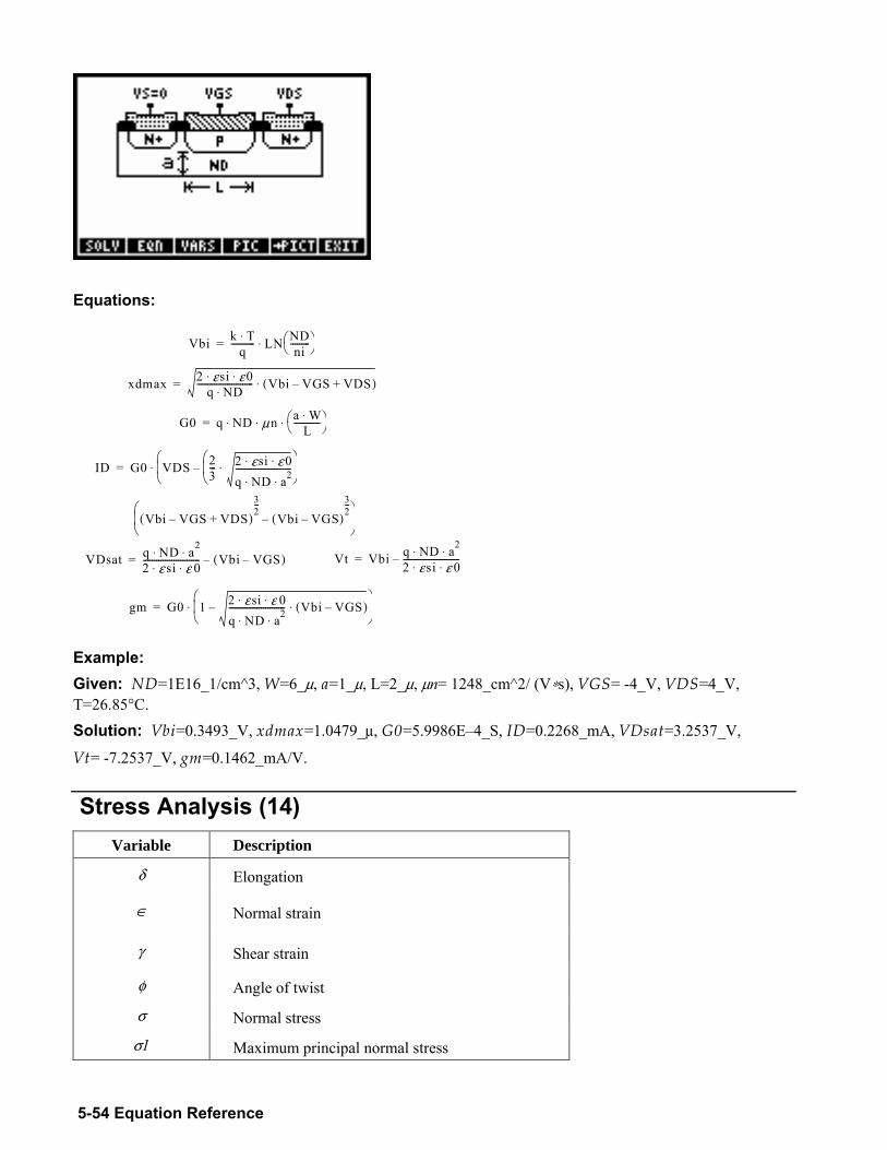
5-54 Equation Reference
Equations:
I D G 0 V D S 2 3 - - - 2 ε s i ε 0 ⋅ ⋅
q N D a 2 ⋅ ⋅ - - - - - - - - - - - - - - - - - - - - - - - - - - ⋅
⎝ ⎠ ⎜ ⎛ ⎞
⎝ ⎜ ⎛
⋅ =
V b i k T ⋅ q - - - - - - - - - - - L N N D
n i - - - - - - - - - ⎝ ⎠ ⎛ ⎞ ⋅ =
V b i V G S V D S + ( ) 3 2 - - -
V b i V G S ( ) 3 2 - - -
⎝ ⎠ ⎜ ⎛ ⎞
V D s a t q N D a 2 ⋅ ⋅ 2 ε s i ε 0 ⋅ ⋅ - - - - - - - - - - - - - - - - - - - - - - - - - - V b i V G S ( ) =
x d m a x 2 ε s i ε 0 ⋅ ⋅ q N D ⋅ - - - - - - - - - - - - - - - - - - - - - - - - - - V b i V G S V DS+ ( )⋅ =
g m G 0 1 2 ε s i ε 0 ⋅ ⋅ q N D a 2 ⋅ ⋅ - - - - - - - - - - - - - - - - -- - - - - - - - - V b i V G S ( )⋅
⎝ ⎠⎜ ⎛ ⎞
⋅ =
V t Vbi q ND a2⋅ ⋅2 εsi ε 0⋅ ⋅--------------------------=
G 0 q N D µ n a W ⋅ L - - - - - - - - - - - - ⎝ ⎠ ⎛ ⎞ ⋅ ⋅ ⋅ =
Example: Given: ND=1E16_1/cm^3, W=6_µ, a=1_µ, L=2_µ, µn= 1248_cm^2/ (V∗s), VGS= -4_V, VDS=4_V, T=26.85°C. Solution: Vbi=0.3493_V, xdmax=1.0479_µ, G0=5.9986E4_S, ID=0.2268_mA, VDsat=3.2537_V,
Vt= -7.2537_V, gm=0.1462_mA/V.
Stress Analysis (14) Variable Description
δ Elongation
∈ Normal strain
γ Shear strain
φ Angle of twist
σ Normal stress
σ1 Maximum principal normal stress
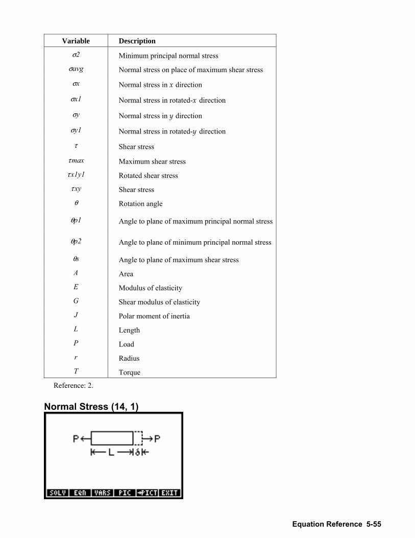
Equation Reference 5-55
Variable Description
σ2 Minimum principal normal stress
σavg Normal stress on place of maximum shear stress
σx Normal stress in x direction
σx1 Normal stress in rotated-x direction
σy Normal stress in y direction
σy1 Normal stress in rotated-y direction
τ Shear stress
τ max Maximum shear stress
τ x1y1 Rotated shear stress
τ xy Shear stress
θ Rotation angle
θp1 Angle to plane of maximum principal normal stress
θp2 Angle to plane of minimum principal normal stress
θs Angle to plane of maximum shear stress
A Area
E Modulus of elasticity
G Shear modulus of elasticity
J Polar moment of inertia
L Length
P Load
r Radius
T Torque
Reference: 2. Normal Stress (14, 1)
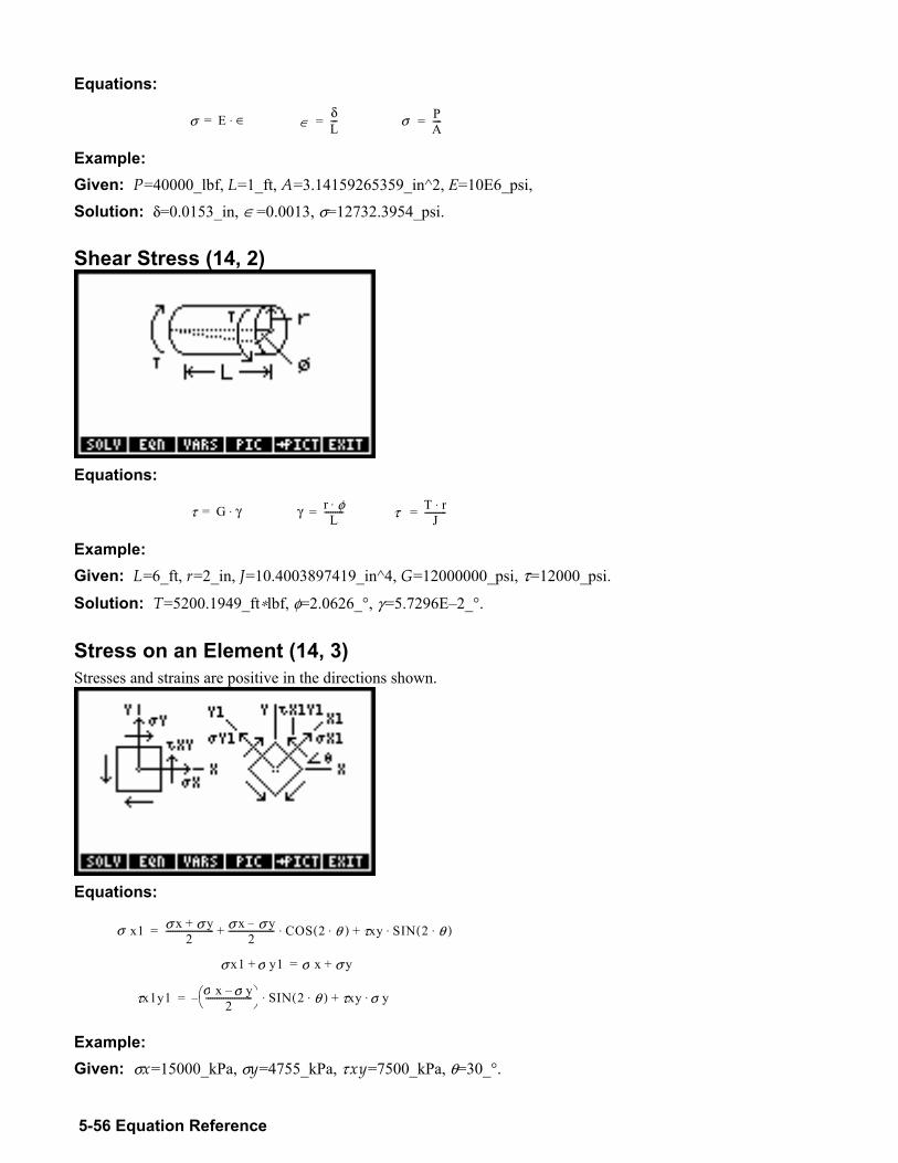
5-56 Equation Reference
Equations:
Example: Given: P=40000_lbf, L=1_ft, A=3.14159265359_in^2, E=10E6_psi,
Solution: δ=0.0153_in, ∈ =0.0013, σ=12732.3954_psi. Shear Stress (14, 2)
Equations:
Example: Given: L=6_ft, r=2_in, J=10.4003897419_in^4, G=12000000_psi, τ=12000_psi.
Solution: T=5200.1949_ft∗lbf, φ=2.0626_°, γ =5.7296E2_°.
Stress on an Element (14, 3) Stresses and strains are positive in the directions shown.
Equations:
Example: Given: σx=15000_kPa, σy=4755_kPa, τ xy=7500_kPa, θ=30_°.
σ E ∈⋅ = ∈ δ L - - - = σ P
A----=
τ G γ ⋅ = γ r φ ⋅ L - - - - - - - - - = τ T r⋅
J----------=
τ x 1 y 1 σ x σ y 2 - - - - - - - - - - - - - - - - - - - - - ⎝ ⎠
⎛ ⎞ S I N 2 θ ⋅ ( ) ⋅ τ x y+ σ y⋅=
σ x 1 σ x σ y + 2 - - - - - - - - - - - - - - - - - - - - - - σ x σ y
2 - - - - - - - - - - - - - - - - - -- - - + C O S 2 θ ⋅ ( ) ⋅ τxy SIN 2 θ⋅( )⋅+ =
σ x 1 σ y 1 + σ x σ y + =
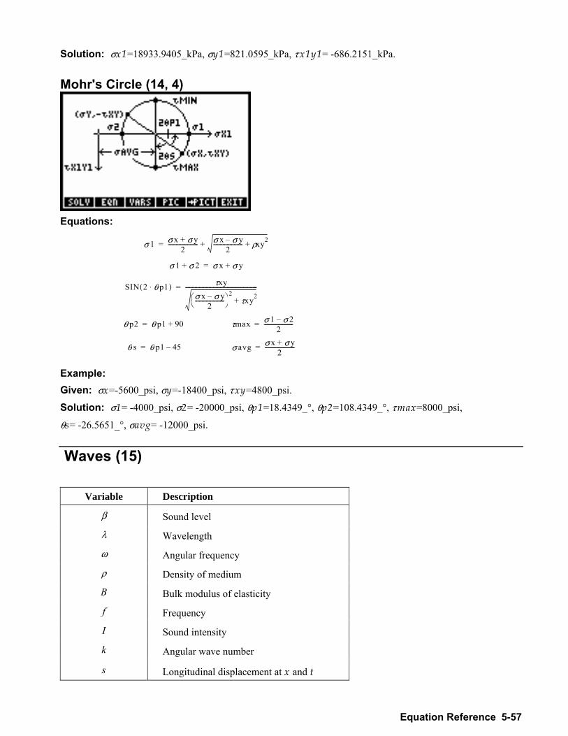
Equation Reference 5-57
Solution: σx1=18933.9405_kPa, σy1=821.0595_kPa, τ x1y1= -686.2151_kPa. Mohr's Circle (14, 4)
Equations:
S I N 2 θ p 1 ⋅ ( ) τ x y σ x σ y
2 - - - - - - - - - - - - - - - - - - - - - ⎝ ⎠ ⎛ ⎞ 2 τxy2+
- - - - - - - - - - - - - - - - - - - - - - - - - - - - - - ----------------------=
σ 1 σ x σ y + 2 -- - - - - - - - - - - - - - - - - - - - - σ x σ y
2- - - - - - - - - - ----------- ρxy2++ =
σ 1 σ 2 + σ x σ y+=
θ p 2 θ p 1 90 + = τmax σ 1 σ 22
---------------------=
θ s θ p 1 45 = σ avg σ x σ y+2
----------------------=
Example: Given: σx=-5600_psi, σy=-18400_psi, τ xy=4800_psi.
Solution: σ1= -4000_psi, σ2= -20000_psi, θp1=18.4349_°, θp2=108.4349_°, τ max=8000_psi,
θs= -26.5651_°, σavg= -12000_psi.
Waves (15)
Variable Description
β Sound level
λ Wavelength
ω Angular frequency
ρ Density of medium
B Bulk modulus of elasticity
f Frequency
I Sound intensity
k Angular wave number
s Longitudinal displacement at x and t
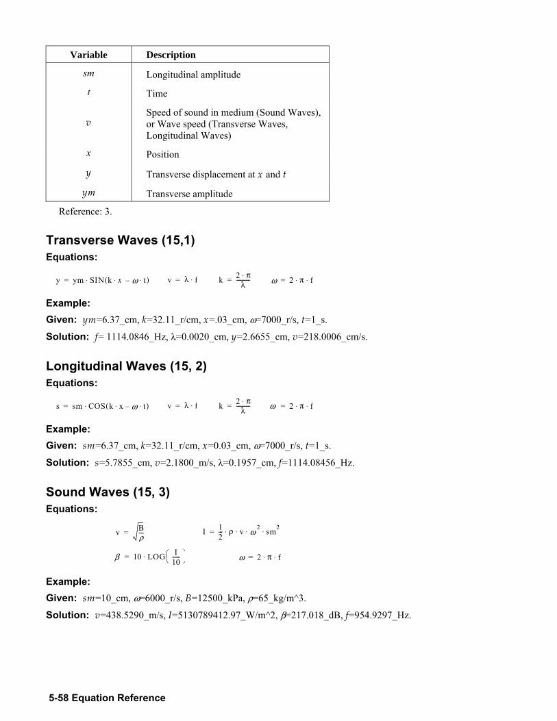
5-58 Equation Reference
Variable Description
sm Longitudinal amplitude
t Time
v Speed of sound in medium (Sound Waves), or Wave speed (Transverse Waves, Longitudinal Waves)
x Position
y Transverse displacement at x and t
ym Transverse amplitude
Reference: 3.
Transverse Waves (15,1) Equations:
Example: Given: ym=6.37_cm, k=32.11_r/cm, x=.03_cm, ω=7000_r/s, t=1_s.
Solution: f= 1114.0846_Hz, λ=0.0020_cm, y=2.6655_cm, v=218.0006_cm/s.
Longitudinal Waves (15, 2) Equations:
Example: Given: sm=6.37_cm, k=32.11_r/cm, x=0.03_cm, ω=7000_r/s, t=1_s.
Solution: s=5.7855_cm, v=2.1800_m/s, λ=0.1957_cm, f=1114.08456_Hz.
Sound Waves (15, 3) Equations:
Example: Given: sm=10_cm, ω=6000_r/s, B=12500_kPa, ρ=65_kg/m^3.
Solution: v=438.5290_m/s, I=5130789412.97_W/m^2, β=217.018_dB, f=954.9297_Hz.
y y m S I N k x⋅ ω t ⋅ ( ) ⋅ = v λ f ⋅ = k 2 π⋅λ----------= ω 2 π f⋅ ⋅=
s s m C O S k x ⋅ ω t ⋅ ( ) ⋅ = v λ f ⋅ = k 2 π⋅λ----------= ω 2 π f⋅ ⋅=
v B ρ - - - - = I 1
2 - - - ρ v ω 2 sm2⋅ ⋅ ⋅ ⋅=
β 10 LO G I 10 - - - - - - ⎝ ⎠
⎛ ⎞ ⋅ = ω 2 π f⋅ ⋅=
Equation Reference 5-59
References 1. Dranchuk, P.M., R.A. Purvis, and D.B. Robinson. "Computer Calculations of Natural Gas Compressibility Factors Using the Standing and Katz Correlation," In Institute of Petroleum Technical Series, no. IP 74-008. 1974.
2. Gere, James M., and Stephen P. Timoshenko. Mechanics of Materials, 2d ed. PWS Engineering, Boston, 1984.
3. Halliday, David, and Robert Resnick. Fundamentals of Physics, 3d ed. John Wiley & Sons, 1988.
4. Meriam, J. L., and L. G. Kraige. Engineering Mechanics, 2d ed. John Wiley & Sons, 1986
5. Muller, Richard S., and Theodore I. Kamins. Device Electronics for Integrated Cicuits, 2d ed. John Wiley & Sons 1986.
6. Serghides, T. K. "Estimate Friction Factor Accurately," In Chemical Engineering, Mar. 5, 1984.
7. Siegel, Robert, and John Howell. Thermal Radiation Heat Transfer, Vol. 1. National Aeronautics and Space Administration, 1968.
8. Sze, S. Physics of Semiconductors, 2d ed. John Wiley & Sons, 1981.
9. Welty, Wicks, and Wilson. Fundamentals of Momentum, Heat and Mass Transfer. John Wiley & Sons, 1969.

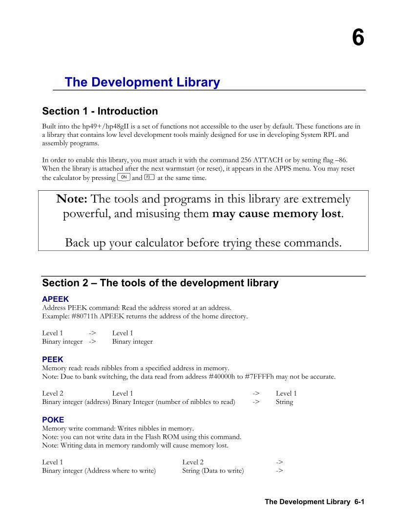
6
The Development Library 6-1
6.The Development Library
Section 1 - Introduction Built into the hp49+/hp48gII is a set of functions not accessible to the user by default. These functions are in a library that contains low level development tools mainly designed for use in developing System RPL and assembly programs. In order to enable this library, you must attach it with the command 256 ATTACH or by setting flag 86. When the library is attached after the next warmstart (or reset), it appears in the APPS menu. You may reset the calculator by pressing $and C at the same time.
Note: The tools and programs in this library are extremely powerful, and misusing them may cause memory lost.
Back up your calculator before trying these commands.
Section 2 The tools of the development library APEEK Address PEEK command: Read the address stored at an address. Example: #80711h APEEK returns the address of the home directory. Level 1 -> Level 1 Binary integer -> Binary integer PEEK Memory read: reads nibbles from a specified address in memory. Note: Due to bank switching, the data read from address #40000h to #7FFFFh may not be accurate. Level 2 Level 1 -> Level 1 Binary integer (address) Binary Integer (number of nibbles to read) -> String POKE Memory write command: Writes nibbles in memory. Note: you can not write data in the Flash ROM using this command. Note: Writing data in memory randomly will cause memory lost. Level 1 Level 2 -> Binary integer (Address where to write) String (Data to write) ->
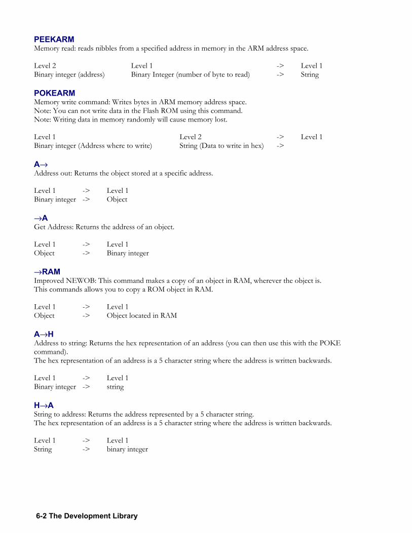
6-2 The Development Library
PEEKARM Memory read: reads nibbles from a specified address in memory in the ARM address space. Level 2 Level 1 -> Level 1 Binary integer (address) Binary Integer (number of byte to read) -> String POKEARM Memory write command: Writes bytes in ARM memory address space. Note: You can not write data in the Flash ROM using this command. Note: Writing data in memory randomly will cause memory lost. Level 1 Level 2 -> Level 1 Binary integer (Address where to write) String (Data to write in hex) -> A→ Address out: Returns the object stored at a specific address. Level 1 -> Level 1 Binary integer -> Object →A Get Address: Returns the address of an object. Level 1 -> Level 1 Object -> Binary integer →RAM Improved NEWOB: This command makes a copy of an object in RAM, wherever the object is. This commands allows you to copy a ROM object in RAM. Level 1 -> Level 1 Object -> Object located in RAM A→H Address to string: Returns the hex representation of an address (you can then use this with the POKE command). The hex representation of an address is a 5 character string where the address is written backwards. Level 1 -> Level 1 Binary integer -> string H→A String to address: Returns the address represented by a 5 character string. The hex representation of an address is a 5 character string where the address is written backwards. Level 1 -> Level 1 String -> binary integer
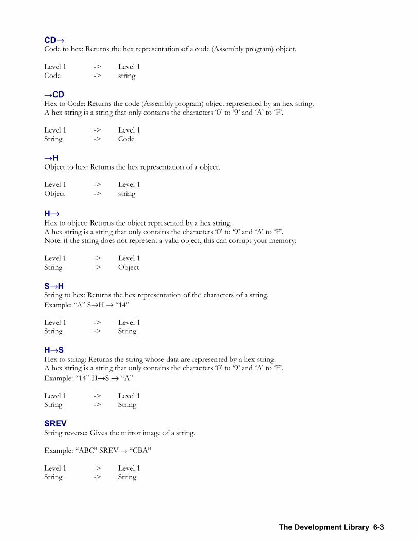
The Development Library 6-3
CD→ Code to hex: Returns the hex representation of a code (Assembly program) object. Level 1 -> Level 1 Code -> string →CD Hex to Code: Returns the code (Assembly program) object represented by an hex string. A hex string is a string that only contains the characters 0 to 9 and A to F. Level 1 -> Level 1 String -> Code →H Object to hex: Returns the hex representation of a object. Level 1 -> Level 1 Object -> string H→ Hex to object: Returns the object represented by a hex string. A hex string is a string that only contains the characters 0 to 9 and A to F. Note: if the string does not represent a valid object, this can corrupt your memory; Level 1 -> Level 1 String -> Object S→H String to hex: Returns the hex representation of the characters of a string. Example: A S→H → 14 Level 1 -> Level 1 String -> String H→S Hex to string: Returns the string whose data are represented by a hex string. A hex string is a string that only contains the characters 0 to 9 and A to F. Example: 14 H→S → A Level 1 -> Level 1 String -> String SREV String reverse: Gives the mirror image of a string. Example: ABC SREV → CBA Level 1 -> Level 1 String -> String
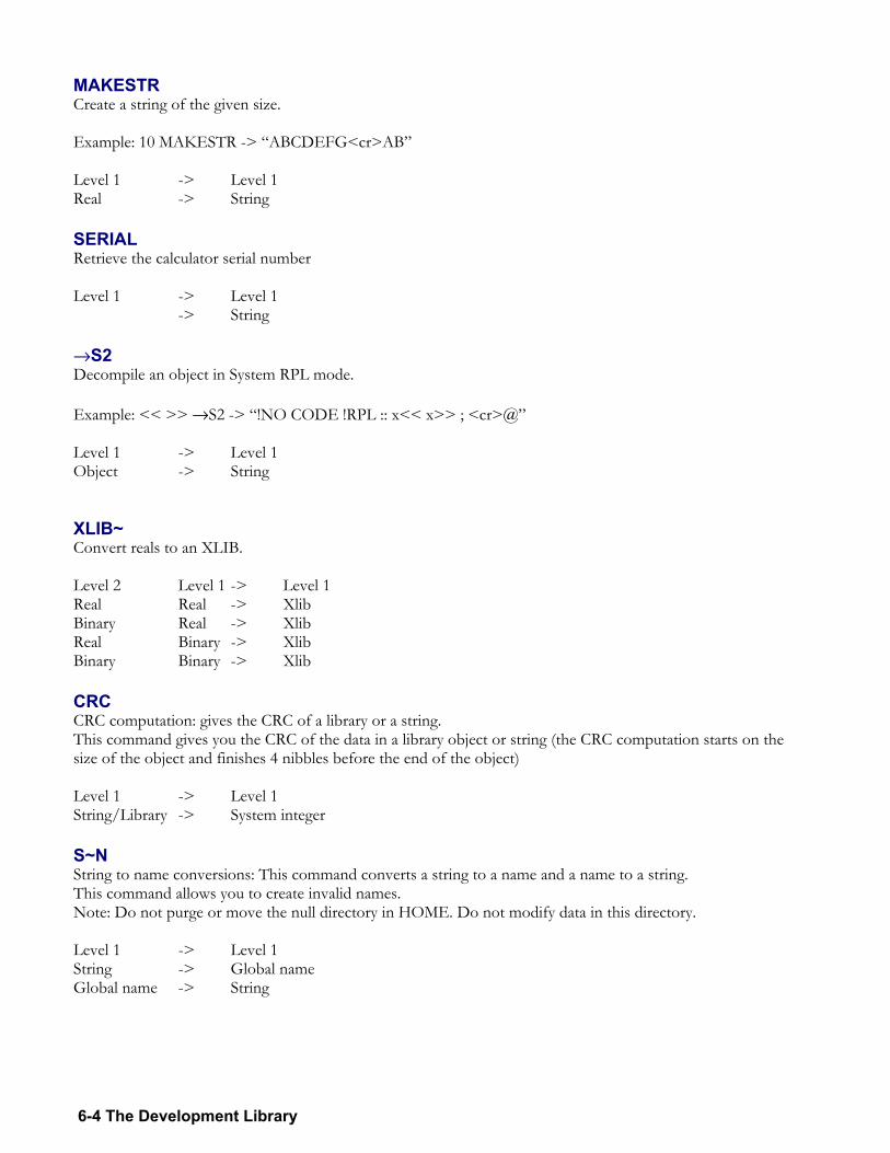
6-4 The Development Library
MAKESTR Create a string of the given size. Example: 10 MAKESTR -> ABCDEFG<cr>AB Level 1 -> Level 1 Real -> String SERIAL Retrieve the calculator serial number Level 1 -> Level 1 -> String →S2 Decompile an object in System RPL mode. Example: << >> →S2 -> !NO CODE !RPL :: x<< x>> ; <cr>@ Level 1 -> Level 1 Object -> String XLIB~ Convert reals to an XLIB. Level 2 Level 1 -> Level 1 Real Real -> Xlib Binary Real -> Xlib Real Binary -> Xlib Binary Binary -> Xlib CRC CRC computation: gives the CRC of a library or a string. This command gives you the CRC of the data in a library object or string (the CRC computation starts on the size of the object and finishes 4 nibbles before the end of the object) Level 1 -> Level 1 String/Library -> System integer S~N String to name conversions: This command converts a string to a name and a name to a string. This command allows you to create invalid names. Note: Do not purge or move the null directory in HOME. Do not modify data in this directory. Level 1 -> Level 1 String -> Global name Global name -> String
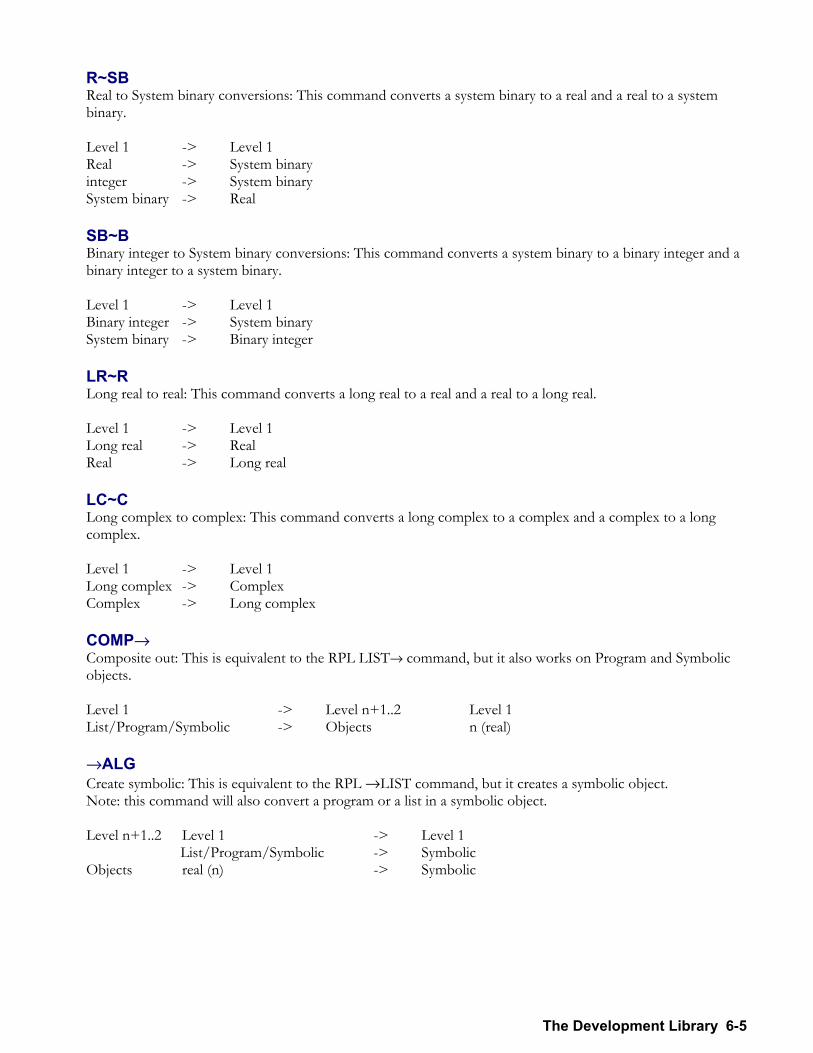
The Development Library 6-5
R~SB Real to System binary conversions: This command converts a system binary to a real and a real to a system binary. Level 1 -> Level 1 Real -> System binary integer -> System binary System binary -> Real SB~B Binary integer to System binary conversions: This command converts a system binary to a binary integer and a binary integer to a system binary. Level 1 -> Level 1 Binary integer -> System binary System binary -> Binary integer LR~R Long real to real: This command converts a long real to a real and a real to a long real. Level 1 -> Level 1 Long real -> Real Real -> Long real LC~C Long complex to complex: This command converts a long complex to a complex and a complex to a long complex. Level 1 -> Level 1 Long complex -> Complex Complex -> Long complex COMP→ Composite out: This is equivalent to the RPL LIST→ command, but it also works on Program and Symbolic objects. Level 1 -> Level n+1..2 Level 1 List/Program/Symbolic -> Objects n (real) →ALG Create symbolic: This is equivalent to the RPL →LIST command, but it creates a symbolic object. Note: this command will also convert a program or a list in a symbolic object. Level n+1..2 Level 1 -> Level 1
List/Program/Symbolic -> Symbolic Objects real (n) -> Symbolic
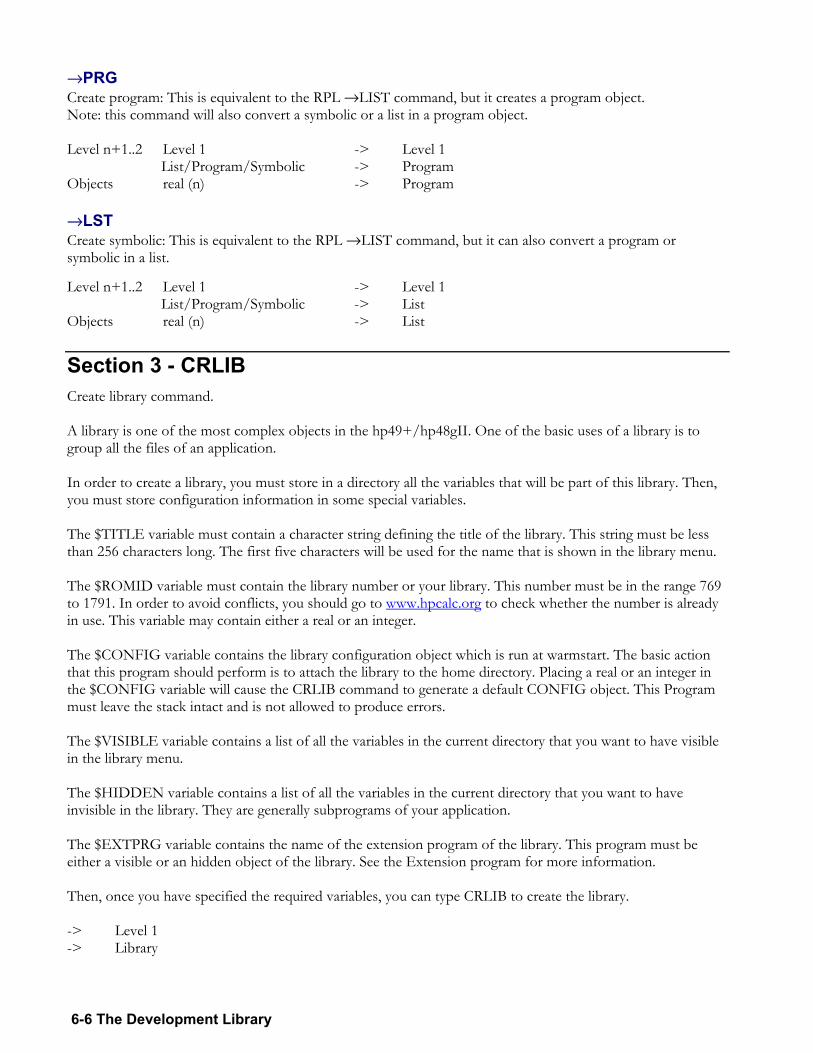
6-6 The Development Library
→PRG Create program: This is equivalent to the RPL →LIST command, but it creates a program object. Note: this command will also convert a symbolic or a list in a program object. Level n+1..2 Level 1 -> Level 1
List/Program/Symbolic -> Program Objects real (n) -> Program →LST Create symbolic: This is equivalent to the RPL →LIST command, but it can also convert a program or symbolic in a list. Level n+1..2 Level 1 -> Level 1
List/Program/Symbolic -> List Objects real (n) -> List
Section 3 - CRLIB Create library command. A library is one of the most complex objects in the hp49+/hp48gII. One of the basic uses of a library is to group all the files of an application. In order to create a library, you must store in a directory all the variables that will be part of this library. Then, you must store configuration information in some special variables. The $TITLE variable must contain a character string defining the title of the library. This string must be less than 256 characters long. The first five characters will be used for the name that is shown in the library menu. The $ROMID variable must contain the library number or your library. This number must be in the range 769 to 1791. In order to avoid conflicts, you should go to HTUwww.hpcalc.orgUTH to check whether the number is already in use. This variable may contain either a real or an integer. The $CONFIG variable contains the library configuration object which is run at warmstart. The basic action that this program should perform is to attach the library to the home directory. Placing a real or an integer in the $CONFIG variable will cause the CRLIB command to generate a default CONFIG object. This Program must leave the stack intact and is not allowed to produce errors. The $VISIBLE variable contains a list of all the variables in the current directory that you want to have visible in the library menu. The $HIDDEN variable contains a list of all the variables in the current directory that you want to have invisible in the library. They are generally subprograms of your application. The $EXTPRG variable contains the name of the extension program of the library. This program must be either a visible or an hidden object of the library. See the Extension program for more information. Then, once you have specified the required variables, you can type CRLIB to create the library. -> Level 1 -> Library
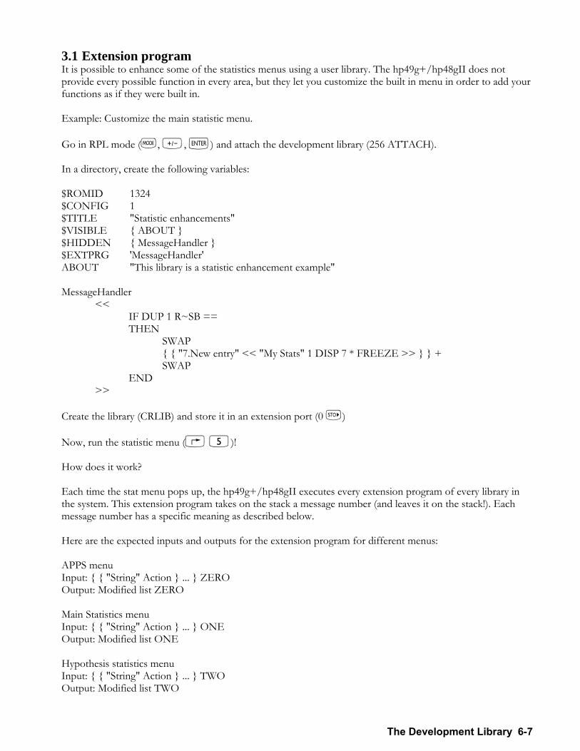
The Development Library 6-7
3.1 Extension program It is possible to enhance some of the statistics menus using a user library. The hp49g+/hp48gII does not provide every possible function in every area, but they let you customize the built in menu in order to add your functions as if they were built in. Example: Customize the main statistic menu. Go in RPL mode (H, W, `) and attach the development library (256 ATTACH). In a directory, create the following variables: $ROMID 1324 $CONFIG 1 $TITLE "Statistic enhancements" $VISIBLE ABOUT $HIDDEN MessageHandler $EXTPRG 'MessageHandler' ABOUT "This library is a statistic enhancement example" MessageHandler
<< IF DUP 1 R~SB == THEN
SWAP "7.New entry" << "My Stats" 1 DISP 7 * FREEZE >> + SWAP
END >>
Create the library (CRLIB) and store it in an extension port (0 K) Now, run the statistic menu (@ 5)! How does it work? Each time the stat menu pops up, the hp49g+/hp48gII executes every extension program of every library in the system. This extension program takes on the stack a message number (and leaves it on the stack!). Each message number has a specific meaning as described below. Here are the expected inputs and outputs for the extension program for different menus: APPS menu Input: "String" Action ... ZERO Output: Modified list ZERO Main Statistics menu Input: "String" Action ... ONE Output: Modified list ONE Hypothesis statistics menu Input: "String" Action ... TWO Output: Modified list TWO
6-8 The Development Library
Confidence interval statistics menu Input: "String" Action ... THREE Output: Modified list THREE Finance menu Input: "String" Action ... FOUR Output: Modified list FOUR Numeric solver menu Input: "String" Action ... FIVE Output: Modified list FIVE
Section 4 - ASM The Machine Language and System RPL Compiler (MASD) 4.1 Introduction 4.1.1 Warnings The operating system can not control what a low level program is doing. Therefore, any programming error is likely to cause the calculator to crash (with potential memory lost). A careful developer will always save source code in the internal flash ROM or port 1 for protection before trying low level programs. This document does not intend to be a programming course it just presents the syntax of the compiler. Ample resources are available on the web (HTUwww.hpcalc.orgUTH) to learn how to program the Saturn CPU in assembler, how to program in System RPL or how to program in ARM assembly. With the introduction of the new ARM based series of calculators, some new things have been included that are not backward compatible with previous calculators. The careful programmer should be wary of this. 4.1.2 Starting MASD To compile a program, put the source code on the level 1 of the stack and type ASM (the development library must be attached) or use the ASM menu of the Development library. If you have a new version of MASD packaged as a library 259, the command to type is asm (note the lowercase). 4.1.3 Modes MASD can be used to compile program in 3 different languages: Saturn ASM, ARM ASM and System RPL. Although some things are common to all modes, some are not. As a programmer, you should always know the current mode. Compilation directives instructions are used to switch from one mode to another: !ASM (switch to Saturn ASM mode, referred in the rest of this document as the Saturn mode) !RPL (switch to System RPL mode) !ARM (switches to ARM ASM mode) In addition, in RPL mode, CODE % here we are in ASM mode ENDCODE Allows switching from RPL mode to Saturn mode (and generate an assembly program object) 4.1.4 Syntax MASD expects a character string (called source) on the stack level 1.
The Development Library 6-9
A source is a set of instructions, comments, and separation characters and ends with a carriage return and an @ character. MASD is case sensitive, so be careful, as «loop» and «LOOP» are two different things for MASD. Separation characters are those with an ASCII number below 32. They include spaces, tabs, line feed and carriage return. In Saturn mode, some instructions need a parameter. Separation characters between an instruction and the parameter are spaces, tabs, and points. Therefore A+B.A can be used instead of A+B A. In ARM mode, parameters for the instruction are separated by spaces and commas. In Saturn or ARM mode, comments can be placed everywhere and begin with % or ; and finish at the end of the current line. In RPL mode, comments are delimited by ( ) as isolated characters and can be multi line. A line that starts with a * on the first character will also be considered a comment. Directives change the way MASD interprets your source. Theses directives begin with a ! and will be explained later. 4.1.5 Errors If MASD detects one or more syntax error, it will push a list describing all errors on the stack. The ER command can help you make sense of that list, point you on the errors and let you correct them. MASD will report a maximum of 16 errors before stopping compilation. The ER command takes 2 objects as arguments:
The original source code (level 2) The error list generated by MASD (level 1)
Normally, you should compile using a process similar to: IFERR ASM THEN ER END (this is what the ASM2 command does BTW). Most peoples will just type the ASM command followed, if error, by the ER command.
4.1.5.1 Format of the error list:
Its a list of at most 16 sub-lists. Each sub-list contains 3 system-binary and 1 global-name. The first system binary is an error message number. The second is an extra system binary used to indicate how too long a jump is. The third one is the position in the source where the error is. The global name is either a NULLNAME if the error was in the main source or the filename of the buggy source.
4.1.5.2 Error messages
Invalid File The file is not a valid source or macro. (must end with a @) Too many You can not do this operation as you are limited to a certain amount of
them (for example, you can not have more than 64 simultaneous skips) Unknown Instruction Unknown instruction Invalid Field Incorrect field Val betw 0-15 expected An integer between 0 and 15 is expected Val betw 1-16 expected An integer between 1 and 16 is expected Val betw 1-8 expected An integer between 1 and 8 is expected Label Expected A label is expected Hexa Expected An hexadecimal number is expected Decimal Expected An decimal number is expected Can't find This object can not be located Label already defined This name is already in use expected A character was expected expected A character was expected (this can happen if you do not close all the
open skips for example) ( expected A ( character was expected [ or ] expected A [ or ] character was expected Forbidden This can not be done Bad Expression This expression is invalid Jump too long This jump is above the limit of the instruction (use a different type of
jump)
6-10 The Development Library
Insuffisant Memory There is not enough memory to compile Matrix Error You can not do this thing here because you are creating a matrix object Define Error You can not do this operation in a DEFINE ARM register expected No comments. ARM invalid imediate In ARM mode, constants must be representable on 8 bit with an even
number of rotation 4.1.6 Links Links are secondary source files that MASD can be directed to compile (equivalent to the $I directive in Pascal and #include in C). As there is no linking phase with MASD (like in C), a multi source project will usually have the form of a main source file that contains a certain number of links. An example of main source would be: " 'Constant_definition 'initialization 'graphic_functions 'other @" When a link call is encountered, MASD suspends compilation of the current source, compiles the new source and then continues compiling the first one. Program and data in the final object will be in the order in which MASD encounters the links. Syntax in ASM and ARM mode: 'FileName links the file called FileName. Syntax in RPL mode: INCLUDE FileName links the file called FileName. Note 1: A link can call other links Note 2: You can not use more than 64 links in your project Note 3: To know how MASD looks for files, see the File search section Note 4: Links are useful to cut projects in independent parts to allow fast and easy access to source code Note 6: It is beneficial to place all constants definitions at the beginning of the compilation process as this will speed up compilation and give more flexibility 4.1.7 Labels A label is a marker in the program. The principal use of labels is to determine jump destinations. A label is a set of less than 64 characters other than space, +, -, * and /. A label begins with a star * and ends with a separation character. Syntax in ASM and ARM mode: *BigLoop is the BigLoop label declaration. Syntax in RPL mode: LABEL BigLoop is the BigLoop label declaration. Be careful about upper and lower cases! Three types of labels can be used:
• Global labels A global label is a label that can be used everywhere in the project, like global variables in Pascal or C.
• Local labels A Local label is a label that is only accessible in a local section like local variables in Pascal or C. A local section starts at the beginning of a source, after a global label or after a link (see link section). A local section finishes at the end of a source, before a link or before a global label. A local label is identified by a . as the first character.
• Link labels A link label is a label that exists only in the link where it is declared, like a private clause in Object Pascal.
The Development Library 6-11
A link label is identified by a _ as the first character. Note 1: In projects, using less global labels is better because a global label takes longer to compile and because it gives a better program structure. A good habit is to use global labels to cut the program in subroutines, and to use local labels inside these subroutines. Note 2: The command line editor is able to find labels in a source. See the GOTO selection in the command line TOOL menu. Note 3: labels in System RPL should only be used by people who know what they are doing. They are only used for fixed address program (absolute mode) which is pretty advanced programming. Note 4: Labels can not be given the same name as constants. 4.1.8 extable extable is an external library that contains a list of constants. This list can be used by MASD as a basic list of constants and is especially useful to the System RPL programmer as most entry points are defined there (like TURNMENUOFF for example). In addition, it also contains a set of supported constants and ASM entry points for the ASM programmer. Please read the extable section in this document to find more information about this library. 4.1.9 Constants Constants are a way for the user to associate a value to an alphanumerical name. This is extremely useful as it makes programs much easier to read and makes them more portable. One of the most popular ways to use constants is to represent memory address for storage of variables. For example, instead of typing D1=80100 every time it is needed, it is better to declare DC Result 80100 at the beginning of the project and then to type D1=(5)Result when needed (it is more portable, more readable and less likely to cause errors). You can create a constant in ASM or ARM mode by doing: DC CstName ExpressionHex or DEFINE CstName ExpressionHex or EQU CstName ExpressionHex In RPL mode, the only valid way to define a constant is: EQU CstName ExpressionHex ExpressionHex is either a hexadecimal number or an expression (starting with a char that can not be confused with the start of a hex number (0..9,A..F). An expression starting with a hexadecimal number can be typed with a leading $, an expression starting with a decimal number can be typed with a leading # character. For an expression starting with a constant that starts with a 0..9 or A..F character, you should put the constant in brackets. Note 1: A constant cannot be given the same name as a label. Note 2: The name of a constant follows the same rules as the name of a label. Note 3: A constant value is stored in 16 nibbles. Note 4: Having constants starting with something that can be interpreted as a hex number, or an ARM register is not a good idea as the compiler might get confused. For example: DC SPFOO 4 MOV R4 SPFOO will generate an error on FOO as the compiler will interpret the mov as a mov from SP to R4. MASD introduces a constant pointer called CP which helps to define constants. CP is defined by: CP=ExpressionHex CP is defined on 5 nibbles, its default value is 80100 (an area of memory that can be used freely by programmers). EQUCP Increment ConstantName Declares a constant with the current CP value and then increase CP by Increment. Note 1: in ASM and ARM mode, DCCP Increment ConstantName is also valid Note 2: Increment is a hexadecimal value, to use a decimal value, put a leading #. For example, if CP equals to $10 EQUCP 5 Foo Defines a Foo constant with a value of $10 and then change the value of CP to $15. Several constants can be defined at once using CP.
6-12 The Development Library
: Inc CstName0 CstName1 ... CstNameN-1 : Defines N constants CstNamex with a value of CP+x*Inc and then changes the CP value to CP+N*Inc. By default, Inc is a decimal number or an expression that can be immediately evaluated. These features are extremely useful to define area of memory for storage of ASM program variables. Note 1: If the entry point library (see related section) is installed on your calculator, all the values in the constant library will be available in your programs the same way than constants are. Note 2: You can define a constant in your program to override the value of an entry in the equation library. 4.1.10 Expressions An expression is a mathematical operation that is calculated at compilation time. Terms of this operation are hexadecimal or decimal values, constants or labels. An expression stops on a separation character or a ]. DCCP 5 @Data ... D1=(5)@Data+$10/#2 D0=(5)$5+DUP LC(5)"DUP"+#5
are correct expressions (provided that the entry point library is installed). Notes:
• A hexadecimal value must begin with a $. • A decimal value may begin with a # or a number directly. • A & or (*) equals the offset of the current instruction in the program (This value has no meaning in
itself, but may be used to calculate the distance between a label and the current instruction). In absolute mode, this represents the final address of the instruction.
• The value of a label is the offset of the label in the program (This value has no meaning in itself, but may be used to calculate the distance between a label and the current instruction). In absolute mode, this represents the final address of the instruction.
• Entries from the EXTABLE may be used. As the EXTABLE does not have the label names limitations with operators, in ambiguous case (DUP+#5 may either be an addition DUP + 5, or an entry DUP+#5), add "" around the word: "DUP"+#5.
• Calculations are done with 64 bits. • X divide by 0 = $FFFFFFFFFFFFFFFF. • In order to avoid wasting memory, MASD tries to compile expressions as soon as it sees them. If MASD
is not able to compile an expression directly, its compiled at the end of the compilation. In order to use less memory, its a good idea to define your constants at the beginning of the sources so MASD can compile expression using the constants directly.
• The only operator symbols not allowed in labels are +, -, * and /; therefore, if you want to use a symbol operator after a label, you must put the symbol between " in order to limit the symbol. Meaningless Example: "DUP"<<5.
• A label/constant with strange char may be protected between " chars. • The evaluation stack of MASD allows you to have around 10 pending computations (parenthesis,
operator priority). • MASD only works with integers. You can represent signed values using standard 2s complement, but be
careful as all operators are unsigned. MASD recognizes the following operators:
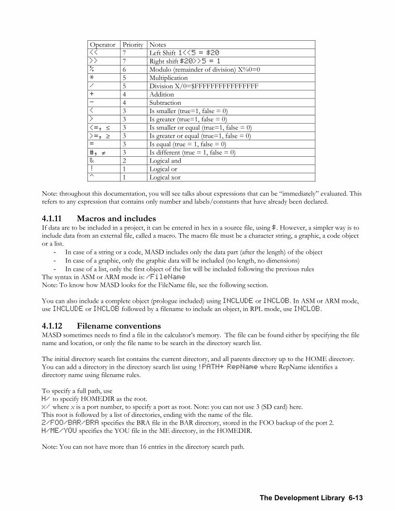
The Development Library 6-13
Operator Priority Notes << 7 Left Shift 1<<5 = $20 >> 7 Right shift $20>>5 = 1 % 6 Modulo (remainder of division) X%0=0 * 5 Multiplication / 5 Division X/0=$FFFFFFFFFFFFFFFF + 4 Addition - 4 Subtraction < 3 Is smaller (true=1, false = 0) > 3 Is greater (true=1, false = 0) <=, ≤ 3 Is smaller or equal (true=1, false = 0) >=, ≥ 3 Is greater or equal (true=1, false = 0) = 3 Is equal (true = 1, false = 0) #, ≠ 3 Is different (true = 1, false = 0) & 2 Logical and ! 1 Logical or ^ 1 Logical xor
Note: throughout this documentation, you will see talks about expressions that can be immediately evaluated. This refers to any expression that contains only number and labels/constants that have already been declared. 4.1.11 Macros and includes If data are to be included in a project, it can be entered in hex in a source file, using $. However, a simpler way is to include data from an external file, called a macro. The macro file must be a character string, a graphic, a code object or a list.
- In case of a string or a code, MASD includes only the data part (after the length) of the object - In case of a graphic, only the graphic data will be included (no length, no dimensions) - In case of a list, only the first object of the list will be included following the previous rules
The syntax in ASM or ARM mode is: /FileName Note: To know how MASD looks for the FileName file, see the following section. You can also include a complete object (prologue included) using INCLUDE or INCLOB. In ASM or ARM mode, use INCLUDE or INCLOB followed by a filename to include an object, in RPL mode, use INCLOB. 4.1.12 Filename conventions MASD sometimes needs to find a file in the calculators memory. The file can be found either by specifying the file name and location, or only the file name to be search in the directory search list. The initial directory search list contains the current directory, and all parents directory up to the HOME directory. You can add a directory in the directory search list using !PATH+ RepName where RepName identifies a directory name using filename rules. To specify a full path, use H/ to specify HOMEDIR as the root. x/ where x is a port number, to specify a port as root. Note: you can not use 3 (SD card) here. This root is followed by a list of directories, ending with the name of the file. 2/FOO/BAR/BRA specifies the BRA file in the BAR directory, stored in the FOO backup of the port 2. H/ME/YOU specifies the YOU file in the ME directory, in the HOMEDIR. Note: You can not have more than 16 entries in the directory search path.
6-14 The Development Library
4.1.13 Compilation directive The following instruction modifies the way MASD reacts and compiles things. They are valid in all modes:
!PATH+ DirName Add the specified directory in the search path list. !NO CODE MASD will not generate a $02DCC prologue but will directly output
the data. If the generated file is not a valid object, an error will be generated.
!DBGON MASD will generate code when DISP or DISPKEY are found in the source.
!DBGOFF MASD will not generate code when DISP or DISPKEY are found in the source.
!1-16 Switch to 1-16 mode. !1-15 Switch to 0-15 mode. !RPL Switch to RPL mode. !ASM Switch to ASM mode. !ARM Switch to ARM mode. !FL=0.a Clear the a compilation flag. !FL=1.a Set the a compilation flag. !?FL=0.a Compile the end of the line if flag a is set. !?FL=1.a Compile the end of the line if flag a is clear. !ABSOLUT Addr Switch to absolute mode. The program begins at the address Addr.
Note: MASD always considers the prolog $02DCC and code length to be the beginning of the program even if !NO CODE is set.
!ABSADR Addr If in absolute mode, add blank nibbles to continue at the specified address. If not possible, errors.
!EVEN In absolute mode, cause an error if the directive is not on an even address.
!ADR MASD will generate a source defining all constants and labels used in the program instead of the program.
!COMPEXP Cause MASD to calculate all previous expressions. !STAT Display/update compilation statistics !DBGINF Causes MASD to generate debugging information (see next section
for more information) !JAZZ See local variable documentation in RPL mode !MASD See local variable documentation in RPL mode
4.1.13.1 The !DBGINF directive If you put the !DBGINF directive into a MASD source, the assembler not only generates your compiled object, but it also returns a string (on level 1) full of debug information. The structure of this string is as follows: 5 DOCSTR 5 Length 5 Number of links (source files) n*[ 2 Number of characters .. Name of link file ] 5 Number of symbols (labels and constants) n*[ 2 Number of characters .. Name of symbol
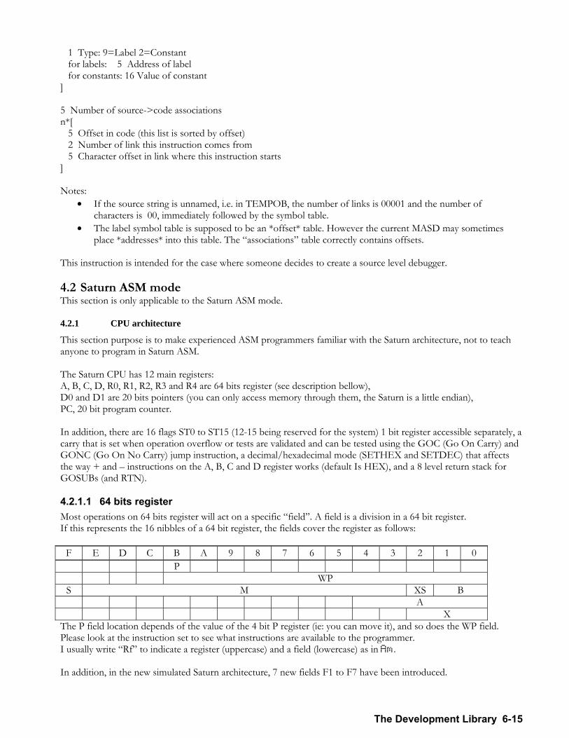
The Development Library 6-15
1 Type: 9=Label 2=Constant for labels: 5 Address of label for constants: 16 Value of constant ] 5 Number of source->code associations n*[ 5 Offset in code (this list is sorted by offset) 2 Number of link this instruction comes from 5 Character offset in link where this instruction starts ] Notes:
• If the source string is unnamed, i.e. in TEMPOB, the number of links is 00001 and the number of characters is 00, immediately followed by the symbol table.
• The label symbol table is supposed to be an *offset* table. However the current MASD may sometimes place *addresses* into this table. The associations table correctly contains offsets.
This instruction is intended for the case where someone decides to create a source level debugger. 4.2 Saturn ASM mode This section is only applicable to the Saturn ASM mode.
4.2.1 CPU architecture
This section purpose is to make experienced ASM programmers familiar with the Saturn architecture, not to teach anyone to program in Saturn ASM. The Saturn CPU has 12 main registers: A, B, C, D, R0, R1, R2, R3 and R4 are 64 bits register (see description bellow), D0 and D1 are 20 bits pointers (you can only access memory through them, the Saturn is a little endian), PC, 20 bit program counter. In addition, there are 16 flags ST0 to ST15 (12-15 being reserved for the system) 1 bit register accessible separately, a carry that is set when operation overflow or tests are validated and can be tested using the GOC (Go On Carry) and GONC (Go On No Carry) jump instruction, a decimal/hexadecimal mode (SETHEX and SETDEC) that affects the way + and instructions on the A, B, C and D register works (default Is HEX), and a 8 level return stack for GOSUBs (and RTN).
4.2.1.1 64 bits register Most operations on 64 bits register will act on a specific field. A field is a division in a 64 bit register. If this represents the 16 nibbles of a 64 bit register, the fields cover the register as follows:
F E D C B A 9 8 7 6 5 4 3 2 1 0 P WP S M XS B A X
The P field location depends of the value of the 4 bit P register (ie: you can move it), and so does the WP field. Please look at the instruction set to see what instructions are available to the programmer. I usually write Rf to indicate a register (uppercase) and a field (lowercase) as in Am. In addition, in the new simulated Saturn architecture, 7 new fields F1 to F7 have been introduced.
6-16 The Development Library
You can define the field mask by using the SETFDLn where n is a number between 1 and 7 to define the field Fn using the mask in Cw as in this example: LC FF000000000000FF SETFLD1 LA 123456789ABCDEF0 LC 0FEDCBA987654321 A=A!C.F1 A is now equal to: 1F3456789ABCDEF1 ie: the instruction on F fields equate to: reg1= (reg1 & ~ mask) | ((reg1 & mask) operation (reg2 & mask)) These new fields are available for all instructions that previously used the so called f encoding and includes the following instructions: Reg=Reg&Reg.f, Reg=Reg!Reg.f, DATx=Reg.f, Reg=DATx.f, Reg=Reg+Cte.f, Reg=Reg-Cte.f, RegSRB.f, RReg=Reg.f, Reg=RReg.f and RegRRegEX.f.
4.2.1.2 Other notes You should read documentations on the internal structure of RPL objects (HTUwww.hpcalc.orgUTH has good documentation) D0, D1, Ba and Da are used by the system (next RPL instruction pointer, RPL stack pointer (@@object on level 1 of the stack), start of free memory and free memory in 5 nibble blocks). The SAVE instruction will save these registers in dedicated memory areas, the LOADRPL instruction will restore them and continue the execution in the system. Please consult documentation on memory map for more information.
4.2.1.3 New instructions In addition to the F fields, the following new instructions have been created: r=s.f, r=r+s.f, r=r-s.f, r=r*s.f, r=r/s.f, r=r%s.f (modulo) r=-s-1.f (logical not), r=-s.f (mathematical not), r=r<s.f (left shift), r=r>s.f (right shift), r=r^s.f (logical xor). r=1.f (alias for r=r/r.f) has also been created. Note 1: any combination of the A, B, C and D registers can be used (notated r and s here) Note 2: all field (including F1-F7 fields) are valid Note 3: MASD will always choose the shortest version of the instruction (e.g.: A=A+B.A will use the standard C0 encoding AND affect the carry) Note 4: the carry is not affected by these instructions. The following other new instructions have been added (see description in the ASM syntax section): NATIVE? $hex GOSLOW REMON CONFIGD HST=1.x WSCREEN SERIAL BIGAPP? ?HST=1.x SETTIME OUTBYT RESETOS SETFLD(1-7) SETLNED MOVEUP REFRESHD OFF SETOFFD MOVEDN AUTOTEST RPL2 HSCREEN ARMSYS ACCESSSD KEYDN UNCNFGD ARMSAT PORTTAG? CRTMP GETTIME REMOFF MIDAPP? BEEP2
4.2.2 Skips
Skips are a first step from ML to a third generation language, even if they are only another way to write ASM instructions. Skips are wonderful as they allow you to:
- structure your program - avoid using gotos - make programs and piece of code that can be easily copied and past (because there is no label)
The foundation of Skips is the Block structure.
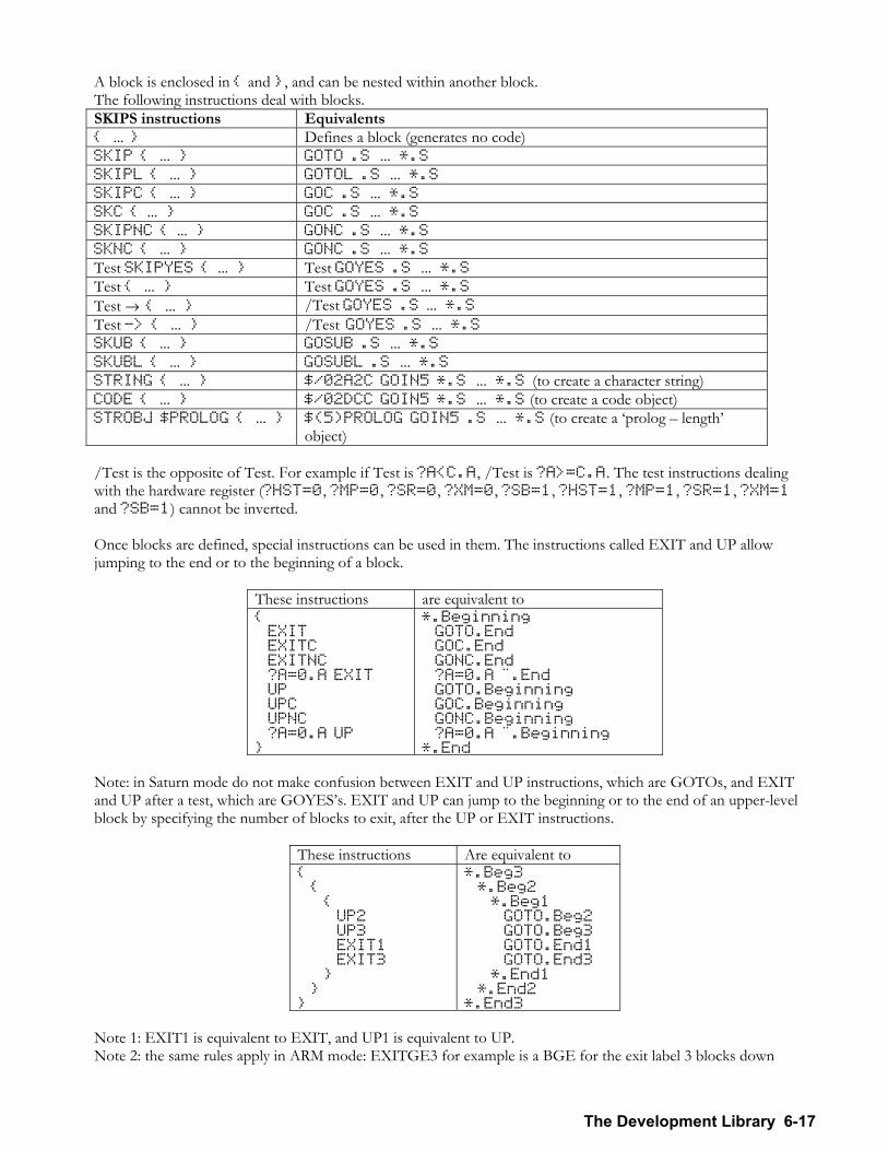
The Development Library 6-17
A block is enclosed in and , and can be nested within another block. The following instructions deal with blocks. SKIPS instructions Equivalents ... Defines a block (generates no code) SKIP ... GOTO .S ... *.S SKIPL ... GOTOL .S ... *.S SKIPC ... GOC .S ... *.S SKC ... GOC .S ... *.S SKIPNC ... GONC .S ... *.S SKNC ... GONC .S ... *.S Test SKIPYES ... Test GOYES .S ... *.S Test ... Test GOYES .S ... *.S Test → ... /Test GOYES .S ... *.S Test -> ... /Test GOYES .S ... *.S SKUB ... GOSUB .S ... *.S SKUBL ... GOSUBL .S ... *.S STRING ... $/02A2C GOIN5 *.S ... *.S (to create a character string) CODE ... $/02DCC GOIN5 *.S ... *.S (to create a code object) STROBJ $PROLOG ... $(5)PROLOG GOIN5 .S ... *.S (to create a prolog length
object) /Test is the opposite of Test. For example if Test is ?A<C.A, /Test is ?A>=C.A. The test instructions dealing with the hardware register (?HST=0, ?MP=0, ?SR=0, ?XM=0, ?SB=1, ?HST=1, ?MP=1, ?SR=1, ?XM=1 and ?SB=1) cannot be inverted. Once blocks are defined, special instructions can be used in them. The instructions called EXIT and UP allow jumping to the end or to the beginning of a block.
These instructions are equivalent to EXIT EXITC EXITNC ?A=0.A EXIT UP UPC UPNC ?A=0.A UP
*.Beginning GOTO.End GOC.End GONC.End ?A=0.A ¨.End GOTO.Beginning GOC.Beginning GONC.Beginning ?A=0.A ¨.Beginning *.End
Note: in Saturn mode do not make confusion between EXIT and UP instructions, which are GOTOs, and EXIT and UP after a test, which are GOYESs. EXIT and UP can jump to the beginning or to the end of an upper-level block by specifying the number of blocks to exit, after the UP or EXIT instructions.
These instructions Are equivalent to UP2 UP3 EXIT1 EXIT3
*.Beg3 *.Beg2 *.Beg1 GOTO.Beg2 GOTO.Beg3 GOTO.End1 GOTO.End3 *.End1 *.End2 *.End3
Note 1: EXIT1 is equivalent to EXIT, and UP1 is equivalent to UP. Note 2: the same rules apply in ARM mode: EXITGE3 for example is a BGE for the exit label 3 blocks down
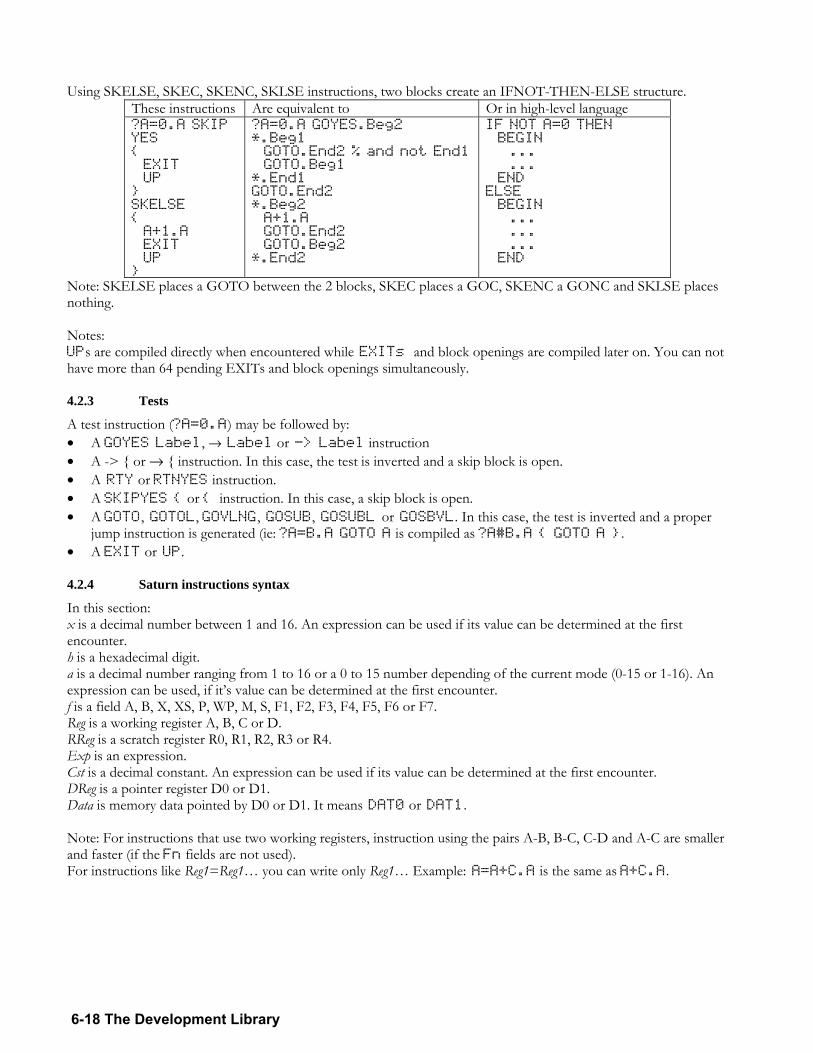
6-18 The Development Library
Using SKELSE, SKEC, SKENC, SKLSE instructions, two blocks create an IFNOT-THEN-ELSE structure.
These instructions Are equivalent to Or in high-level language ?A=0.A SKIPYES EXIT UP SKELSE A+1.A EXIT UP
?A=0.A GOYES.Beg2 *.Beg1 GOTO.End2 % and not End1 GOTO.Beg1 *.End1 GOTO.End2 *.Beg2 A+1.A GOTO.End2 GOTO.Beg2 *.End2
IF NOT A=0 THEN BEGIN ... ... END ELSE BEGIN ... ... ... END
Note: SKELSE places a GOTO between the 2 blocks, SKEC places a GOC, SKENC a GONC and SKLSE places nothing. Notes: UPs are compiled directly when encountered while EXITs and block openings are compiled later on. You can not have more than 64 pending EXITs and block openings simultaneously.
4.2.3 Tests
A test instruction (?A=0.A) may be followed by: • A GOYES Label, → Label or -> Label instruction • A -> or → instruction. In this case, the test is inverted and a skip block is open. • A RTY or RTNYES instruction. • A SKIPYES or instruction. In this case, a skip block is open. • A GOTO, GOTOL, GOVLNG, GOSUB, GOSUBL or GOSBVL. In this case, the test is inverted and a proper
jump instruction is generated (ie: ?A=B.A GOTO A is compiled as ?A#B.A GOTO A . • A EXIT or UP.
4.2.4 Saturn instructions syntax
In this section: x is a decimal number between 1 and 16. An expression can be used if its value can be determined at the first encounter. h is a hexadecimal digit. a is a decimal number ranging from 1 to 16 or a 0 to 15 number depending of the current mode (0-15 or 1-16). An expression can be used, if its value can be determined at the first encounter. f is a field A, B, X, XS, P, WP, M, S, F1, F2, F3, F4, F5, F6 or F7. Reg is a working register A, B, C or D. RReg is a scratch register R0, R1, R2, R3 or R4. Exp is an expression. Cst is a decimal constant. An expression can be used if its value can be determined at the first encounter. DReg is a pointer register D0 or D1. Data is memory data pointed by D0 or D1. It means DAT0 or DAT1. Note: For instructions that use two working registers, instruction using the pairs A-B, B-C, C-D and A-C are smaller and faster (if the Fn fields are not used). For instructions like Reg1=Reg1 you can write only Reg1 Example: A=A+C.A is the same as A+C.A.
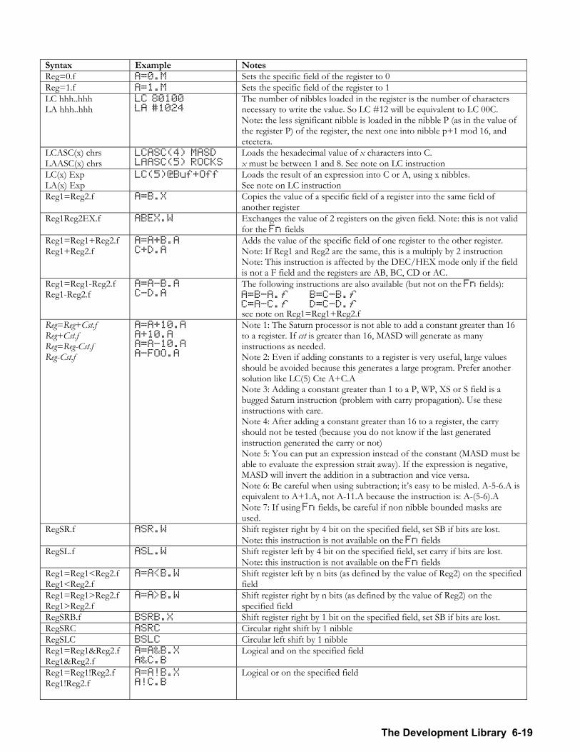
The Development Library 6-19
Syntax Example Notes Reg=0.f A=0.M Sets the specific field of the register to 0 Reg=1.f A=1.M Sets the specific field of the register to 1 LC hhh..hhh LA hhh..hhh
LC 80100 LA #1024
The number of nibbles loaded in the register is the number of characters necessary to write the value. So LC #12 will be equivalent to LC 00C. Note: the less significant nibble is loaded in the nibble P (as in the value of the register P) of the register, the next one into nibble p+1 mod 16, and etcetera.
LCASC(x) chrs LAASC(x) chrs
LCASC(4) MASD LAASC(5) ROCKS
Loads the hexadecimal value of x characters into C. x must be between 1 and 8. See note on LC instruction
LC(x) Exp LA(x) Exp
LC(5)@Buf+Off Loads the result of an expression into C or A, using x nibbles. See note on LC instruction
Reg1=Reg2.f A=B.X Copies the value of a specific field of a register into the same field of another register
Reg1Reg2EX.f ABEX.W Exchanges the value of 2 registers on the given field. Note: this is not valid for the Fn fields
Reg1=Reg1+Reg2.f Reg1+Reg2.f
A=A+B.A C+D.A
Adds the value of the specific field of one register to the other register. Note: If Reg1 and Reg2 are the same, this is a multiply by 2 instruction Note: This instruction is affected by the DEC/HEX mode only if the field is not a F field and the registers are AB, BC, CD or AC.
Reg1=Reg1-Reg2.f Reg1-Reg2.f
A=A-B.A C-D.A
The following instructions are also available (but not on the Fn fields): A=B-A.f B=C-B.f C=A-C.f D=C-D.f see note on Reg1=Reg1+Reg2.f
Reg=Reg+Cst.f Reg+Cst.f Reg=Reg-Cst.f Reg-Cst.f
A=A+10.A A+10.A A=A-10.A A-FOO.A
Note 1: The Saturn processor is not able to add a constant greater than 16 to a register. If cst is greater than 16, MASD will generate as many instructions as needed. Note 2: Even if adding constants to a register is very useful, large values should be avoided because this generates a large program. Prefer another solution like LC(5) Cte A+C.A Note 3: Adding a constant greater than 1 to a P, WP, XS or S field is a bugged Saturn instruction (problem with carry propagation). Use these instructions with care. Note 4: After adding a constant greater than 16 to a register, the carry should not be tested (because you do not know if the last generated instruction generated the carry or not) Note 5: You can put an expression instead of the constant (MASD must be able to evaluate the expression strait away). If the expression is negative, MASD will invert the addition in a subtraction and vice versa. Note 6: Be careful when using subtraction; its easy to be misled. A-5-6.A is equivalent to A+1.A, not A-11.A because the instruction is: A-(5-6).A Note 7: If using Fn fields, be careful if non nibble bounded masks are used.
RegSR.f ASR.W Shift register right by 4 bit on the specified field, set SB if bits are lost. Note: this instruction is not available on the Fn fields
RegSL.f ASL.W Shift register left by 4 bit on the specified field, set carry if bits are lost. Note: this instruction is not available on the Fn fields
Reg1=Reg1<Reg2.f Reg1<Reg2.f
A=A<B.W Shift register left by n bits (as defined by the value of Reg2) on the specified field
Reg1=Reg1>Reg2.f Reg1>Reg2.f
A=A>B.W Shift register right by n bits (as defined by the value of Reg2) on the specified field
RegSRB.f BSRB.X Shift register right by 1 bit on the specified field, set SB if bits are lost. RegSRC ASRC Circular right shift by 1 nibble RegSLC BSLC Circular left shift by 1 nibble Reg1=Reg1&Reg2.f Reg1&Reg2.f
A=A&B.X A&C.B
Logical and on the specified field
Reg1=Reg1!Reg2.f Reg1!Reg2.f
A=A!B.X A!C.B
Logical or on the specified field
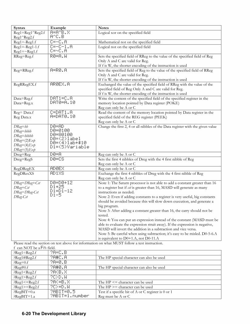
6-20 The Development Library
Syntax Example Notes Reg1=Reg1^Reg2.f Reg1^Reg2.f
A=A^B.X A^C.B
Logical xor on the specified field
Reg1=-Reg1.f C=-C.A Mathematical not on the specified field Reg1=-Reg1-1.f Reg1=~Reg1.f
C=-C-1.A C=~C.A
Logical not on the specified field
RReg=Reg.f R0=A.W Sets the specified field of RReg to the value of the specified field of Reg Only A and C are valid for Reg. If f is W, the shorter encoding of the instruction is used
Reg=RReg.f A=R0.A Sets the specified field of Reg to the value of the specified field of RReg Only A and C are valid for Reg. If f is W, the shorter encoding of the instruction is used
RegRRegEX.f AR0EX.A Exchanged the value of the specified field of RReg with the value of the specified field of Reg Only A and C are valid for Reg. If f is W, the shorter encoding of the instruction is used
Data=Reg.f Data=Reg.x
DAT1=C.A DAT0=A.10
Write the content of the specified field of the specified register in the memory location pointed by Data register (POKE) Reg can only be A or C
Reg= Data.f Reg Data.x
C=DAT1.A A=DAT0.10
Read the content of the memory location pointed by Data register in the specified field of the REG register (PEEK) Reg can only be A or C
DReg=hh DReg=hhhh DReg=hhhhh DReg=(2)Exp DReg=(4)Exp DReg=(5)Exp
D0=AD D0=0100 D0=80100 D0=(2)label D0=(4)lab+$10 D1=(5)Variable
Change the first 2, 4 or all nibbles of the Data register with the given value
Dreg=Reg D0=A Reg can only be A or C Dreg=RegS D0=CS Sets the first 4 nibbles of Dreg with the 4 first nibble of Reg
Reg can only be A or C RegDRegEX AD0EX Reg can only be A or C RegDRexXS AD1XS Exchange the first 4 nibbles of Dreg with the 4 first nibble of Reg
Reg can only be A or C DReg=DReg+Cst DReg+Cst DReg=DReg-Cst DReg-Cst
D0=D0+12 D1+25 D1=D1-12 D1-5
Note 1: The Saturn processor is not able to add a constant greater than 16 to a register but if cst is greater than 16, MASD will generate as many instructions as needed. Note 2: Even if adding constants to a register is very useful, big constants should be avoided because this will slow down execution, and generate a big program. Note 3: After adding a constant greater than 16, the carry should not be tested. Note 4: You can put an expression instead of the constant (MASD must be able to evaluate the expression strait away). If the expression is negative, MASD will invert the addition in a subtraction and vice versa. Note 5: Be careful when using subtraction; its easy to be misled. D0-5-6.A is equivalent to D0+1.A, not D0-11.A
Please read the section on test above for information on what MUST follow a test instruction. f can NOT be a Fn field. ?Reg1=Reg2.f ?A=C.B ?Reg1#Reg2.f ?A#C.A The HP special character can also be used ?Reg=0.f ?A=0.B ?Reg#0.f ?A#0.A The HP special character can also be used ?Reg1<Reg2.f ?A<B.X ?Reg1>Reg2.f ?C>D.W ?Reg1<=Reg2.f ?A<=B.X The HP <= character can be used ?Reg1>=Reg2.f ?C>=D.W The HP >= character can be used ?RegBIT=0.a ?RegBIT=1.a
?ABIT=0.5 ?ABIT=1.number
Test if a specific bit of A or C register is 0 or 1 Reg must be A or C
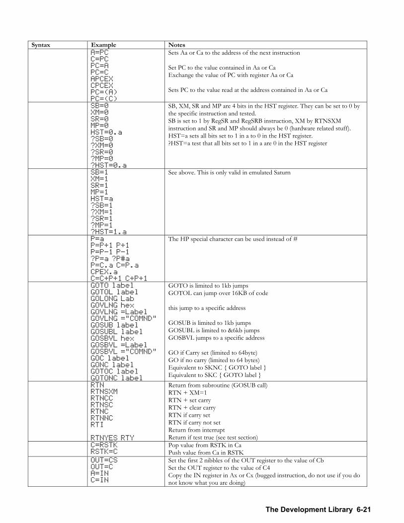
The Development Library 6-21
Syntax Example Notes A=PC
C=PC PC=A PC=C APCEX CPCEX PC=(A) PC=(C)
Sets Aa or Ca to the address of the next instruction Set PC to the value contained in Aa or Ca Exchange the value of PC with register Aa or Ca Sets PC to the value read at the address contained in Aa or Ca
SB=0 XM=0 SR=0 MP=0 HST=0.a ?SB=0 ?XM=0 ?SR=0 ?MP=0 ?HST=0.a
SB, XM, SR and MP are 4 bits in the HST register. They can be set to 0 by the specific instruction and tested. SB is set to 1 by RegSR and RegSRB instruction, XM by RTNSXM instruction and SR and MP should always be 0 (hardware related stuff). HST=a sets all bits set to 1 in a to 0 in the HST register. ?HST=a test that all bits set to 1 in a are 0 in the HST register
SB=1 XM=1 SR=1 MP=1 HST=a ?SB=1 ?XM=1 ?SR=1 ?MP=1 ?HST=1.a
See above. This is only valid in emulated Saturn
P=a P=P+1 P+1 P=P-1 P-1 ?P=a ?P#a P=C.a C=P.a CPEX.a C=C+P+1 C+P+1
The HP special character can be used instead of #
GOTO label GOTOL label GOLONG Lab GOVLNG hex GOVLNG =Label GOVLNG ="COMND" GOSUB label GOSUBL label GOSBVL hex GOSBVL =Label GOSBVL ="COMND" GOC label GONC label GOTOC label GOTONC label
GOTO is limited to 1kb jumps GOTOL can jump over 16KB of code this jump to a specific address GOSUB is limited to 1kb jumps GOSUBL is limited to &6kb jumps GOSBVL jumps to a specific address GO if Carry set (limited to 64byte) GO if no carry (limited to 64 bytes) Equivalent to SKNC GOTO label Equivalent to SKC GOTO label
RTN RTNSXM RTNCC RTNSC RTNC RTNNC RTI RTNYES RTY
Return from subroutine (GOSUB call) RTN + XM=1 RTN + set carry RTN + clear carry RTN if carry set RTN if carry not set Return from interrupt Return if test true (see test section)
C=RSTK RSTK=C
Pop value from RSTK in Ca Push value from Ca in RSTK
OUT=CS OUT=C A=IN C=IN
Set the first 2 nibbles of the OUT register to the value of Cb Set the OUT register to the value of C4 Copy the IN register in Ax or Cx (bugged instruction, do not use if you do not know what you are doing)
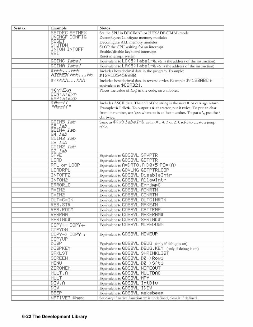
6-22 The Development Library
Syntax Example Notes SETDEC SETHEX
UNCNGF CONFIG RESET SHUTDN INTON INTOFF RSI
Set the SPU in DECIMAL or HEXADECIMAL mode Deconfigure/Configure memory modules Deconfigure ALL memory modules STOP the CPU waiting for an interrupt Enable/disable keyboard interrupts Reset interrupt system
GOINC label Equivalent to LC(5)label-&. (& is the address of the instruction) GOINA label Equivalent to LA(5)label-& (& is the address of the instruction) $hhh...hhh
NIBHEX hhh...hh Includes hexadecimal data in the program. Example: $12ACD545680B.
$/hhhh...hhh Includes hexadecimal data in reverse order. Example: $/123ABC is equivalent to $CBA321.
$(x)Exp CON(x)Exp EXP(x)Exp
Places the value of Exp in the code, on x nibbles.
¢Ascii "Ascii"
Includes ASCII data. The end of the string is the next ¢ or carriage return. Example: ¢Hello¢. To output a ¢ character, put it twice. To put an char from its number, use \xx where xx is an hex number. To put a \, put the \ chr twice.
GOIN5 lab G5 lab GOIN4 lab G4 lab GOIN3 lab G3 lab GOIN2 lab G2 lab
Same as $(x)label-& with x=5, 4, 3 or 2. Useful to create a jump table.
SAVE Equivalent to GOSBVL SAVPTR LOAD Equivalent to GOSBVL GETPTR RPL or LOOP Equivalent to A=DAT0.A D0+5 PC=(A) LOADRPL Equivalent to GOVLNG GETPTRLOOP INTOFF2 Equivalent to GOSBVL DisableIntr INTON2 Equivalent to GOSBVL AllowIntr ERROR_C Equivalent to GOSBVL ErrjmpC A=IN2 Equivalent to GOSBVL AINRTN C=IN2 Equivalent to GOSBVL CINRTN OUT=C=IN Equivalent to GOSBVL OUTCINRTN RES.STR Equivalent to GOSBVL MAKE$N RES.ROOM Equivalent to GOSBVL GETTEMP RESRAM Equivalent to GOSBVL MAKERAM$ SHRINK$ Equivalent to GOSBVL SHRINK$ COPY<- COPY←
COPYDN Equivalent to GOSBVL MOVEDOWN
COPY-> COPY→ COPYUP
Equivalent to GOSBVL MOVEUP
DISP Equivalent to GOSBVL DBUG (only if debug is on) DISPKEY Equivalent to GOSBVL DBUG.KEY (only if debug is on) SRKLST Equivalent to GOSBVL SHRINKLIST SCREEN Equivalent to GOSBVL D0->Row1 MENU Equivalent to GOSBVL D0->Sft1 ZEROMEM Equivalent to GOSBVL WIPEOUT MULT.A Equivalent to GOSBVL MULTBAC MULT Equivalent to GOSBVL MPY DIV.A Equivalent to GOSBVL IntDiv DIV Equivalent to GOSBVL IDIV BEEP Equivalent to GOSBVL makebeep NATIVE? $hex Set carry if native function xx is undefined, clear it if defined.
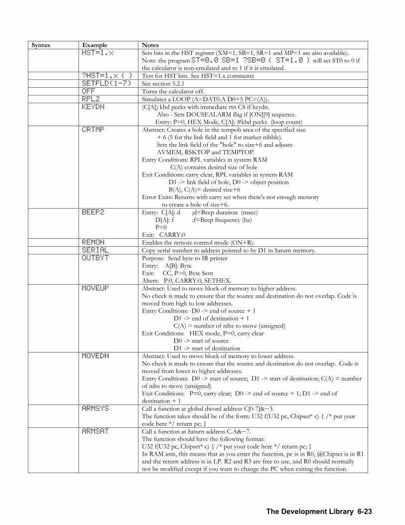
The Development Library 6-23
Syntax Example Notes HST=1.x Sets bits in the HST register (XM=1, SB=1, SR=1 and MP=1 are also available).
Note: the program ST=0.0 SB=1 ?SB=0 ST=1.0 will set ST0 to 0 if the calculator is non-emulated and to 1 if it is emulated.
?HST=1.x Test for HST bits. See HST=1.x comments SETFLD(1-7) See section 5.2.1 OFF Turns the calculator off. RPL2 Simulates a LOOP (A=DAT0.A D0+5 PC=(A)). KEYDN (C[A]) kbd peeks with immediate rtn CS if keydn.
Also - Sets DOUSEALARM flag if [ON][9] sequence. Entry: P=0, HEX Mode, C[A]: #kbd peeks (loop count)
CRTMP Abstract: Creates a hole in the tempob area of the specified size + 6 (5 for the link field and 1 for marker nibble). Sets the link field of the "hole" to size+6 and adjusts AVMEM, RSKTOP and TEMPTOP. Entry Conditions: RPL variables in system RAM C(A) contains desired size of hole Exit Conditions: carry clear, RPL variables in system RAM D1 -> link field of hole, D0 -> object position B(A), C(A)= desired size+6 Error Exits: Returns with carry set when there's not enough memory to create a hole of size+6.
BEEP2 Entry: C[A]: d ;d=Beep duration (msec) D[A]: f ;f=Beep frequency (hz) P=0 Exit: CARRY:0
REMON Enables the remote control mode (ON+R). SERIAL Copy serial number to address pointed to by D1 in Saturn memory. OUTBYT Purpose: Send byte to IR printer
Entry: A[B]: Byte Exit: CC, P=0, Byte Sent Alters: P:0, CARRY:0, SETHEX.
MOVEUP Abstract: Used to move block of memory to higher address. No check is made to ensure that the source and destination do not overlap. Code is moved from high to low addresses. Entry Conditions: D0 -> end of source + 1 D1 -> end of destination + 1 C(A) = number of nibs to move (unsigned) Exit Conditions: HEX mode, P=0, carry clear D0 -> start of source D1 -> start of destination
MOVEDN Abstract: Used to move block of memory to lower address. No check is made to ensure that the source and destination do not overlap. Code is moved from lower to higher addresses. Entry Conditions: D0 -> start of source; D1 -> start of destination; C(A) = number of nibs to move (unsigned) Exit Conditions: P=0, carry clear; D0 -> end of source + 1; D1 -> end of destination + 1
ARMSYS Call a function at global dword address C[0-7]&~3. The function takes should be of the form: U32 f(U32 pc, Chipset* c) /* put your code here */ return pc;
ARMSAT Call a function at Saturn address C.A&~7. The function should have the following format: U32 f(U32 pc, Chipset* c) /* put your code here */ return pc; In RAM asm, this means that as you enter the function, pc is in R0, @Chipset is in R1 and the return address is in LP. R2 and R3 are free to use, and R0 should normally not be modified except if you want to change the PC when exiting the function.
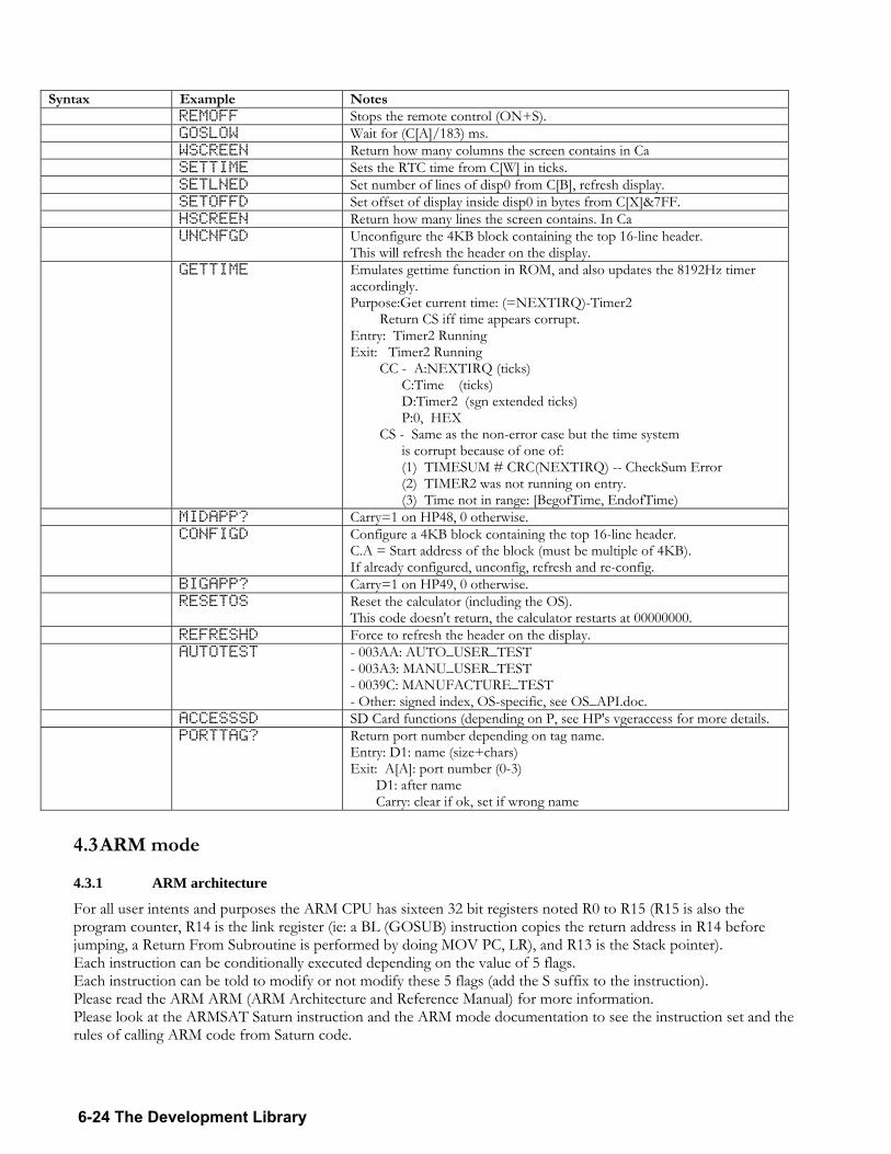
6-24 The Development Library
Syntax Example Notes REMOFF Stops the remote control (ON+S). GOSLOW Wait for (C[A]/183) ms. WSCREEN Return how many columns the screen contains in Ca SETTIME Sets the RTC time from C[W] in ticks. SETLNED Set number of lines of disp0 from C[B], refresh display. SETOFFD Set offset of display inside disp0 in bytes from C[X]&7FF. HSCREEN Return how many lines the screen contains. In Ca UNCNFGD Unconfigure the 4KB block containing the top 16-line header.
This will refresh the header on the display. GETTIME Emulates gettime function in ROM, and also updates the 8192Hz timer
accordingly. Purpose:Get current time: (=NEXTIRQ)-Timer2 Return CS iff time appears corrupt. Entry: Timer2 Running Exit: Timer2 Running CC - A:NEXTIRQ (ticks) C:Time (ticks) D:Timer2 (sgn extended ticks) P:0, HEX CS - Same as the non-error case but the time system is corrupt because of one of: (1) TIMESUM # CRC(NEXTIRQ) -- CheckSum Error (2) TIMER2 was not running on entry. (3) Time not in range: [BegofTime, EndofTime)
MIDAPP? Carry=1 on HP48, 0 otherwise. CONFIGD Configure a 4KB block containing the top 16-line header.
C.A = Start address of the block (must be multiple of 4KB). If already configured, unconfig, refresh and re-config.
BIGAPP? Carry=1 on HP49, 0 otherwise. RESETOS Reset the calculator (including the OS).
This code doesn't return, the calculator restarts at 00000000. REFRESHD Force to refresh the header on the display. AUTOTEST - 003AA: AUTO_USER_TEST
- 003A3: MANU_USER_TEST - 0039C: MANUFACTURE_TEST - Other: signed index, OS-specific, see OS_API.doc.
ACCESSSD SD Card functions (depending on P, see HP's vgeraccess for more details. PORTTAG? Return port number depending on tag name.
Entry: D1: name (size+chars) Exit: A[A]: port number (0-3) D1: after name Carry: clear if ok, set if wrong name
4.3 ARM mode
4.3.1 ARM architecture
For all user intents and purposes the ARM CPU has sixteen 32 bit registers noted R0 to R15 (R15 is also the program counter, R14 is the link register (ie: a BL (GOSUB) instruction copies the return address in R14 before jumping, a Return From Subroutine is performed by doing MOV PC, LR), and R13 is the Stack pointer). Each instruction can be conditionally executed depending on the value of 5 flags. Each instruction can be told to modify or not modify these 5 flags (add the S suffix to the instruction). Please read the ARM ARM (ARM Architecture and Reference Manual) for more information. Please look at the ARMSAT Saturn instruction and the ARM mode documentation to see the instruction set and the rules of calling ARM code from Saturn code.
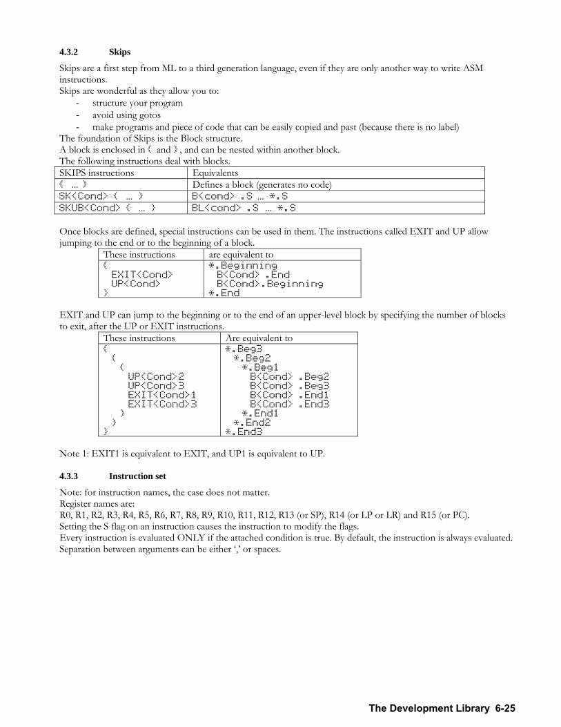
The Development Library 6-25
4.3.2 Skips
Skips are a first step from ML to a third generation language, even if they are only another way to write ASM instructions. Skips are wonderful as they allow you to:
- structure your program - avoid using gotos - make programs and piece of code that can be easily copied and past (because there is no label)
The foundation of Skips is the Block structure. A block is enclosed in and , and can be nested within another block. The following instructions deal with blocks. SKIPS instructions Equivalents ... Defines a block (generates no code) SK<Cond> ... B<cond> .S ... *.S SKUB<Cond> ... BL<cond> .S ... *.S Once blocks are defined, special instructions can be used in them. The instructions called EXIT and UP allow jumping to the end or to the beginning of a block.
These instructions are equivalent to EXIT<Cond> UP<Cond>
*.Beginning B<Cond> .End B<Cond>.Beginning *.End
EXIT and UP can jump to the beginning or to the end of an upper-level block by specifying the number of blocks to exit, after the UP or EXIT instructions.
These instructions Are equivalent to UP<Cond>2 UP<Cond>3 EXIT<Cond>1 EXIT<Cond>3
*.Beg3 *.Beg2 *.Beg1 B<Cond> .Beg2 B<Cond> .Beg3 B<Cond> .End1 B<Cond> .End3 *.End1 *.End2 *.End3
Note 1: EXIT1 is equivalent to EXIT, and UP1 is equivalent to UP.
4.3.3 Instruction set
Note: for instruction names, the case does not matter. Register names are: R0, R1, R2, R3, R4, R5, R6, R7, R8, R9, R10, R11, R12, R13 (or SP), R14 (or LP or LR) and R15 (or PC). Setting the S flag on an instruction causes the instruction to modify the flags. Every instruction is evaluated ONLY if the attached condition is true. By default, the instruction is always evaluated. Separation between arguments can be either , or spaces.
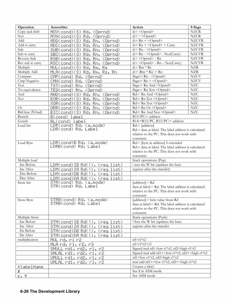
6-26 The Development Library
Operation Assembler Action S flags Copy and shift MOVcondS Rd, <Oprnd> d:= <Oprnd> NZCR Not MVNcondS Rd, <Oprnd> d:= ~<Oprnd> NZCR Add ADDcondS Rd, Rn, <Oprnd> d:= Rn + <Oprnd> NZCVR Add w carry ADCcondS Rd, Rn, <Oprnd> d:= Rn + <Oprnd> + Carry NZCVR Sub SUBcondS Rd, Rn, <Oprnd> d:= Rn - <Oprnd> NZCVR Sub w carry SBCcondS Rd, Rn, <Oprnd> d:= Rn - <Oprnd> - Not(Carry) NZCVR Reverse Sub RSBcondS Rd, Rn, <Oprnd> d:= <Oprnd> - Rn NZCVR Rev sub w carry RSCcondS Rd, Rn, <Oprnd> d:= <Oprnd> - Rn Not(Carry) NZCVR Multiply MULcondS Rd, Rm, Rs d:= Rm * Rs NZR Multiply Add MLAcondS Rd, Rm, Rs, Rn d:= (Rm * Rs) + Rn NZR Compare CMPcond Rd, <Oprnd> flags:= Rn - <Oprnd> NZCV Cmp Negative CMNcond Rd, <Oprnd> flags:= Rn + <Oprnd> NZCV Test TSTcond Rn, <Oprnd> flags:= Rn And <Oprnd> NZC Tst equivalence TEQcond Rn, <Oprnd> flags:= Rn Xor <Oprnd> NZC And ANDcondS Rd, Rn, <Oprnd> Rd:= Rn And <Oprnd> NZC Xor EORcondS Rd, Rn, <Oprnd> Rd:= Rn Xor <Oprnd> NZC XORcondS Rd, Rn, <Oprnd> Rd:= Rn Xor <Oprnd> NZC Or ORRcondS Rd, Rn, <Oprnd> Rd:= Rn Or <Oprnd> NZC BitClear (ÑAnd) BICcondS Rd, Rn, <Oprnd> Rd:= Rn And Not <Oprnd> NZC Branch Bcond label R15/PC:= address Gosub BLcond label R14:=R15/PC, R15/PC:= address Load Int LDRcond Rd, <a_mode>
LDRcond Rd, Label Rd:= [address] Rd:= data at label. The label address is calculated relative to the PC. This does not work with constants
Load Byte LDRcondB Rd, <a_mode> LDRBcond Rd, Label
Rd:= [byte at address] 0 extended Rd:= data at label. The label address is calculated relative to the PC. This does not work with constants
Multiple load Stack operations (Pop) Inc Before LDMcondIB Rd!, reg list ! sets the W bit (updates the base Inc After LDMcondIA Rd!, reg list register after the transfer) Dec Before LDMcondDB Rd!, reg list Dec After LDMcondDA Rd!, reg list Store Int STRcond Rd, <a_mode>
STRcond Rd, Label [address]:= Rd data at label:= Rd. The label address is calculated relative to the PC. This does not work with constants
Store Byte STRBcond Rd, <a_mode> STRBcond Rd, Label
[address]:= byte value from Rd data at label:= Rd. The label address is calculated relative to the PC. This does not work with constants
Multiple Store Stack operations (Push) Inc Before STMcondIB Rd!, reg list ! Sets the W bit (updates the base Inc After STMcondIA Rd!, reg list register after the transfer De Before STMcondDB Rd!, reg list De After STMcondDA Rd!, reg list multiplication MUL rd, r1 r2 rd=r1*r2 MLA rd, r1, r2, r3 rd=r1*r2+r3 SMULL rd1, rd2, r1, r2 Signed mul rd1=low r1*r2, rd2=high r1*r2 SMLAL rd1, rd2, r1, r2 Signed mul add rd1+=low r1*r2, rd2+=high r1*r2 UMULL rd1, rd2, r1, r2 rd1=low r1*r2, rd2=high r1*r2 UMLAL rd1, rd2, r1, r2 mul add rd1+=low r1*r2, rd2+=high r1*r2 *labelName Creates a label $ See $ in ASM mode “, ¢ See ASM mode
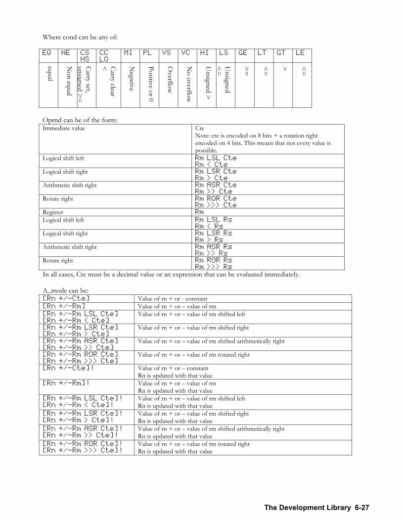
The Development Library 6-27
Where cond can be any of: EQ NE CS
HS CC LO
MI PL VS VC HI LS GE LT GT LE
equal
Non equal
Carry set, unsi gned >
=
Carry clear <
Negative
Positive or 0
Overflow
No overflow
Unsigned >
Unsigned
<=
>=
<=
>
<=
Oprnd can be of the form: Immediate value Cte
Note: cte is encoded on 8 bits + a rotation right encoded on 4 bits. This means that not every value is possible.
Logical shift left Rm LSL Cte Rm < Cte
Logical shift right Rm LSR Cte Rm > Cte
Arithmetic shift right Rm ASR Cte Rm >> Cte
Rotate right Rm ROR Cte Rm >>> Cte
Register Rm Logical shift left Rm LSL Rs
Rm < Rs Logical shift right Rm LSR Rs
Rm > Rs Arithmetic shift right Rm ASR Rs
Rm >> Rs Rotate right Rm ROR Rs
Rm >>> Rs In all cases, Cte must be a decimal value or an expression that can be evaluated immediately. A_mode can be: [Rn +/-Cte] Value of rn + or - constant [Rn +/-Rm] Value of rn + or value of rm [Rn +/-Rm LSL Cte] [Rn +/-Rm < Cte]
Value of rn + or value of rm shifted left
[Rn +/-Rm LSR Cte] [Rn +/-Rm > Cte]
Value of rn + or value of rm shifted right
[Rn +/-Rm ASR Cte] [Rn +/-Rm >> Cte]
Value of rn + or value of rm shifted arithmetically right
[Rn +/-Rm ROR Cte] [Rn +/-Rm >>> Cte]
Value of rn + or value of rm rotated right
[Rn +/-Cte]! Value of rn + or constant Rn is updated with that value
[Rn +/-Rm]! Value of rn + or value of rm Rn is updated with that value
[Rn +/-Rm LSL Cte]! [Rn +/-Rm < Cte]!
Value of rn + or value of rm shifted left Rn is updated with that value
[Rn +/-Rm LSR Cte]! [Rn +/-Rm > Cte]!
Value of rn + or value of rm shifted right Rn is updated with that value
[Rn +/-Rm ASR Cte]! [Rn +/-Rm >> Cte]!
Value of rn + or value of rm shifted arithmetically right Rn is updated with that value
[Rn +/-Rm ROR Cte]! [Rn +/-Rm >>> Cte]!
Value of rn + or value of rm rotated right Rn is updated with that value
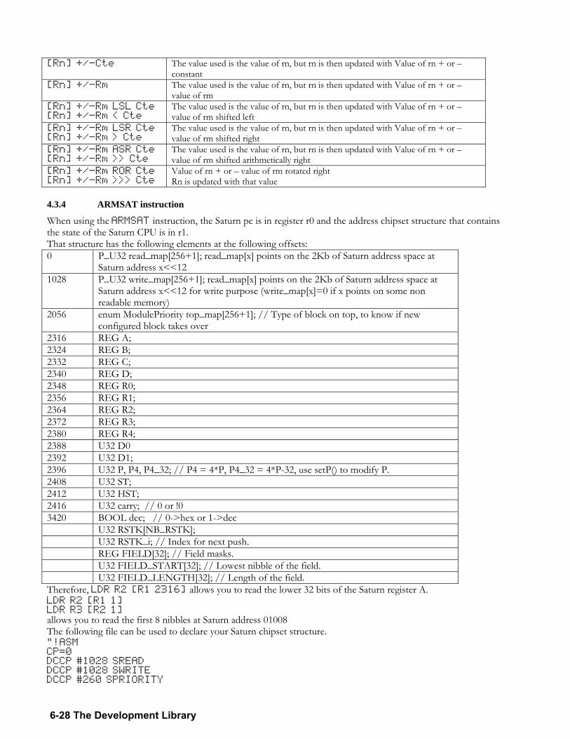
6-28 The Development Library
[Rn] +/-Cte The value used is the value of rn, but rn is then updated with Value of rn + or
constant [Rn] +/-Rm The value used is the value of rn, but rn is then updated with Value of rn + or
value of rm [Rn] +/-Rm LSL Cte [Rn] +/-Rm < Cte
The value used is the value of rn, but rn is then updated with Value of rn + or value of rm shifted left
[Rn] +/-Rm LSR Cte [Rn] +/-Rm > Cte
The value used is the value of rn, but rn is then updated with Value of rn + or value of rm shifted right
[Rn] +/-Rm ASR Cte [Rn] +/-Rm >> Cte
The value used is the value of rn, but rn is then updated with Value of rn + or value of rm shifted arithmetically right
[Rn] +/-Rm ROR Cte [Rn] +/-Rm >>> Cte
Value of rn + or value of rm rotated right Rn is updated with that value
4.3.4 ARMSAT instruction
When using the ARMSAT instruction, the Saturn pc is in register r0 and the address chipset structure that contains the state of the Saturn CPU is in r1. That structure has the following elements at the following offsets: 0 P_U32 read_map[256+1]; read_map[x] points on the 2Kb of Saturn address space at
Saturn address x<<12 1028 P_U32 write_map[256+1]; read_map[x] points on the 2Kb of Saturn address space at
Saturn address x<<12 for write purpose (write_map[x]=0 if x points on some non readable memory)
2056 enum ModulePriority top_map[256+1]; // Type of block on top, to know if new configured block takes over
2316 REG A; 2324 REG B; 2332 REG C; 2340 REG D; 2348 REG R0; 2356 REG R1; 2364 REG R2; 2372 REG R3; 2380 REG R4; 2388 U32 D0 2392 U32 D1; 2396 U32 P, P4, P4_32; // P4 = 4*P, P4_32 = 4*P-32, use setP() to modify P. 2408 U32 ST; 2412 U32 HST; 2416 U32 carry; // 0 or !0 3420 BOOL dec; // 0->hex or 1->dec U32 RSTK[NB_RSTK]; U32 RSTK_i; // Index for next push. REG FIELD[32]; // Field masks. U32 FIELD_START[32]; // Lowest nibble of the field. U32 FIELD_LENGTH[32]; // Length of the field. Therefore, LDR R2 [R1 2316] allows you to read the lower 32 bits of the Saturn register A. LDR R2 [R1 1] LDR R3 [R2 1] allows you to read the first 8 nibbles at Saturn address 01008 The following file can be used to declare your Saturn chipset structure. "!ASM CP=0 DCCP #1028 SREAD DCCP #1028 SWRITE DCCP #260 SPRIORITY
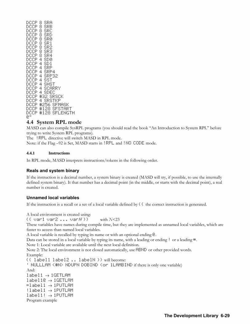
The Development Library 6-29
DCCP 8 SRA DCCP 8 SRB DCCP 8 SRC DCCP 8 SRD DCCP 8 SR0 DCCP 8 SR1 DCCP 8 SR2 DCCP 8 SR3 DCCP 8 SR4 DCCP 4 SD0 DCCP 4 SD1 DCCP 4 SRP DCCP 4 SRP4 DCCP 4 SRP32 DCCP 4 SST DCCP 4 SHST DCCP 4 SCARRY DCCP 4 SDEC DCCP #32 SRSCK DCCP 4 SRSTKP DCCP #256 SFMASK DCCP #128 SFSTART DCCP #128 SFLENGTH @"
4.4 System RPL mode MASD can also compile SysRPL programs (you should read the book An Introduction to System RPL before trying to write System RPL programs). The !RPL directive will switch MASD in RPL mode. Note: if the Flag 92 is Set, MASD starts in !RPL and !NO CODE mode.
4.4.1 Instructions
In RPL mode, MASD interprets instructions/tokens in the following order.
Reals and system binary If the instruction is a decimal number, a system binary is created (MASD will try, if possible, to use the internally defined system binary). It that number has a decimal point (in the middle, or starts with the decimal point), a real number is created.
Unnamed local variables If the instruction is a recall or a set of a local variable defined by the correct instruction is generated. A local environment is created using: var1 var2 ... varN with N<23 These variables have names during compile time, but they are implemented as unnamed local variables, which are faster to access than named local variables. A local variable is recalled by typing its name or with an optional ending @. Data can be stored in a local variable by typing its name, with a leading or ending ! or a leading =. Note 1: Local variable are available until the next local definition. Note 2: The local environment is not closed automatically, use ABND or other provided words. Example: label1 label2 .. labelN will become: ' NULLLAM <#N> NDUPN DOBIND (or 1LAMBIND if there is only one variable) And: label1 → 1GETLAM label1@ → 1GETLAM =label1 → 1PUTLAM !label1 → 1PUTLAM label1! → 1PUTLAM Program example
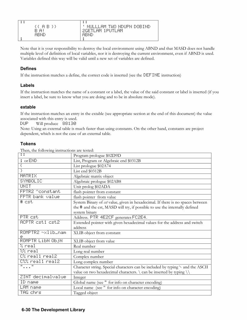
6-30 The Development Library
:: A B B A! ABND ;
:: ' NULLLAM TWO NDUPN DOBIND 2GETLAM 1PUTLAM ABND ;
Note that it is your responsibility to destroy the local environment using ABND and that MASD does not handle multiple level of definition of local variables, nor it is destroying the current environment, even if ABND is used. Variables defined this way will be valid until a new set of variables are defined.
Defines If the instruction matches a define, the correct code is inserted (see the DEFINE instruction)
Labels If the instruction matches the name of a constant or a label, the value of the said constant or label is inserted (if you insert a label, be sure to know what you are doing and to be in absolute mode).
extable If the instruction matches an entry in the extable (see appropriate section at the end of this document) the value associated with this entry is used. DUP Will produce 88130 Note: Using an external table is much faster than using constants. On the other hand, constants are project dependent, which is not the case of an external table.
Tokens Then, the following instructions are tested: :: Program prologue $02D9D ; or END List, Program or Algebraic end $0312B List prologue $02A74 List end $0312B MATRIX Algebraic matrix object SYMBOLIC Algebraic prologue $02AB8 UNIT Unit prolog $02ADA FPTR2 ^constant flash pointer from constant FPTR bank value flash pointer from value # cst System Binary of cst value, given in hexadecimal. If there is no spaces between
the # and the cst, MASD will try, if possible to use the internally defined system binary
PTR cst Address. PTR 4E2CF generates FC2E4. ACPTR cst1 cst2 Extended pointer with given hexadecimal values for the address and switch
address ROMPTR2 ~xlib_name
XLIB object from constant
ROMPTR LibN ObjN XLIB object from value % real Real number %% real Long real number C% real1 real2 Complex number C%% real1 real2 Long complex number "..." Character string. Special characters can be included by typing \ and the ASCII
value on two hexadecimal characters. \ can be inserted by typing \\ ZINT decimalvalue Integer ID name Global name (see " for info on character encoding) LAM name Local name (see " for info on character encoding) TAG chrs Tagged object
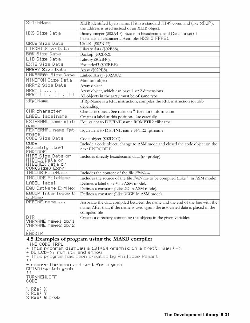
The Development Library 6-31
XxlibName XLIB identified by its name. If it is a standard HP49 command (like xDUP), the address is used instead of an XLIB object.
HXS Size Data Binary integer ($02A4E), Size is in hexadecimal and Data is a set of hexadecimal characters. Example: HXS 5 FFA21
GROB Size Data GROB ($02B1E). LIBDAT Size Data Library data ($02B88). BAK Size Data Backup ($02B62). LIB Size Data Library ($02B40). EXT3 Size Data Extended3 ($02BEE). ARRAY Size Data Array ($029E8). LNKARRAY Size Data Linked Array ($02A0A). MINIFON Size Data Minifont object ARRY2 Size Data Array object ARRY [ ... ] ARRY [ [ . ] [ . ] ]
Array object, which can have 1 or 2 dimensions. All objects in the array must be of same type
xRplName If RplName is a RPL instruction, compiles the RPL instruction (or xlib depending)
CHR character Character object. See rules on " for more information LABEL labelname Creates a label at this position. Use carefully EXTERNAL name xlibname
Equivalent to DEFINE name ROMPTR2 xlibname
FEXTERNAL name fptrname
Equivalent to DEFINE name FPTR2 fptrname
CODE Size Data Code object ($02DCC). CODE Assembly stuff ENDCODE
Include a code object, change to ASM mode and closed the code object on the next ENDCODE.
NIBB Size Data or NIBHEX Data or NIBBHEX Data or CON(Size) Expr
Includes directly hexadecimal data (no prolog).
INCLOB FileName Includes the content of the file FileName. INCLUDE FileName Includes the source of the file FileName to be compiled (Like ' in ASM mode). LABEL label Defines a label (like * in ASM mode). EQU CstName ExpHex Defines a constant (Like DC in ASM mode). EQUCP Interleave CstName
Defines a constant (Like DCCP in ASM mode).
DEFINE name ... Associate the data compiled between the name and the end of the line with the name. After that, if the name is used again, the associated data is placed in the compiled file
DIR VARNAME name1 obj1 VARNAME name2 obj2 ... ENDDIR
Creates a directory containing the objects in the given variables.
4.5 Examples of program using the MASD compiler "!NO CODE !RPL * This program display a 131*64 graphic in a pretty way :-) * DO LCD->, run it, and enjoy! * This program has been created by Philippe Pamart :: * remove the menu and test for a grob CK1&Dispatch grob :: TURNMENUOFF CODE % R0a: X % R1a: Y % R2a: @ grob
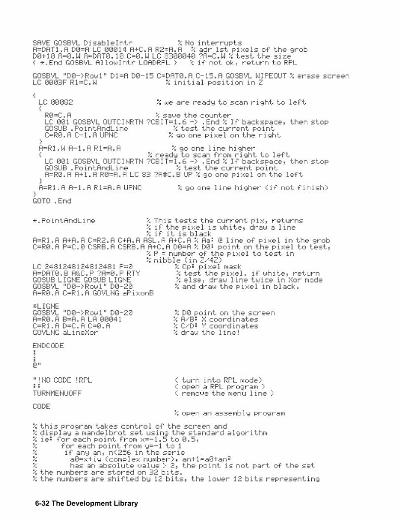
6-32 The Development Library
SAVE GOSBVL DisableIntr % No interrupts A=DAT1.A D0=A LC 00014 A+C.A R2=A.A % adr 1st pixels of the grob D0+10 A=0.W A=DAT0.10 C=0.W LC 8300040 ?A=C.W % test the size *.End GOSBVL AllowIntr LOADRPL % if not ok, return to RPL GOSBVL "D0->Row1" D1=A D0-15 C=DAT0.A C-15.A GOSBVL WIPEOUT % erase screen LC 0003F R1=C.W % initial position in Z LC 00082 % we are ready to scan right to left R0=C.A % save the counter LC 001 GOSBVL OUTCINRTN ?CBIT=1.6 -> .End % If backspace, then stop GOSUB .PointAndLine % test the current point C=R0.A C-1.A UPNC % go one pixel on the right A=R1.W A-1.A R1=A.A % go one line higher % ready to scan from right to left LC 001 GOSBVL OUTCINRTN ?CBIT=1.6 -> .End % If backspace, then stop GOSUB .PointAndLine % test the current point A=R0.A A+1.A R0=A.A LC 83 ?A#C.B UP % go one pixel on the left A=R1.A A-1.A R1=A.A UPNC % go one line higher (if not finish) GOTO .End *.PointAndLine % This tests the current pix, returns % if the pixel is white, draw a line % if it is black A=R1.A A+A.A C=R2.A C+A.A ASL.A A+C.A % Aa: @ line of pixel in the grob C=R0.A P=C.0 CSRB.A CSRB.A A+C.A D0=A % D0: point on the pixel to test, % P = number of the pixel to test in % nibble (in Z/4Z) LC 2481248124812481 P=0 % Cp: pixel mask A=DAT0.B A&C.P ?A=0.P RTY % test the pixel. if white, return GOSUB LIGNE GOSUB LIGNE % else, draw line twice in Xor mode GOSBVL "D0->Row1" D0-20 % and draw the pixel in black. A=R0.A C=R1.A GOVLNG aPixonB *LIGNE GOSBVL "D0->Row1" D0-20 % D0 point on the screen A=R0.A B=A.A LA 00041 % A/B: X coordinates C=R1.A D=C.A C=0.A % C/D: Y coordinates GOVLNG aLineXor % draw the line! ENDCODE ; ; @" "!NO CODE !RPL ( turn into RPL mode) :: ( open a RPL program ) TURNMENUOFF ( remove the menu line ) CODE % open an assembly program % this program takes control of the screen and % display a mandelbrot set using the standard algorithm % ie: for each point from x=-1.5 to 0.5, % for each point from y=-1 to 1 % if any an, n<256 in the serie % a0=x+iy (complex number), an+1=a0+an² % has an absolute value > 2, the point is not part of the set % the numbers are stored on 32 bits. % the numbers are shifted by 12 bits, the lower 12 bits representing
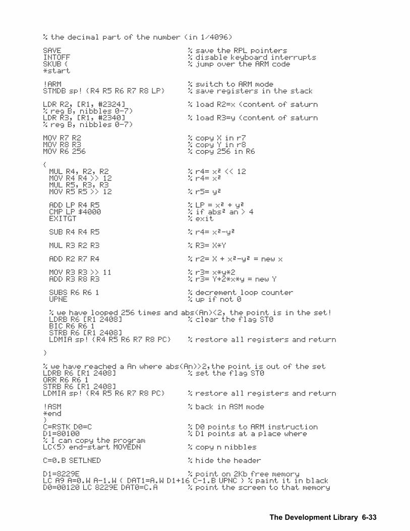
The Development Library 6-33
% the decimal part of the number (in 1/4096) SAVE % save the RPL pointers INTOFF % disable keyboard interrupts SKUB % jump over the ARM code *start !ARM % switch to ARM mode STMDB sp! R4 R5 R6 R7 R8 LP % save registers in the stack LDR R2, [R1, #2324] % load R2=x (content of saturn % reg B, nibbles 0-7) LDR R3, [R1, #2340] % load R3=y (content of saturn % reg B, nibbles 0-7) MOV R7 R2 % copy X in r7 MOV R8 R3 % copy Y in r8 MOV R6 256 % copy 256 in R6 MUL R4, R2, R2 % r4= x² << 12 MOV R4 R4 >> 12 % r4= x² MUL R5, R3, R3 MOV R5 R5 >> 12 % r5= y² ADD LP R4 R5 % LP = x² + y² CMP LP $4000 % if abs² an > 4 EXITGT % exit SUB R4 R4 R5 % r4= x²-y² MUL R3 R2 R3 % R3= X*Y ADD R2 R7 R4 % r2= X + x²-y² = new x MOV R3 R3 >> 11 % r3= x*y*2 ADD R3 R8 R3 % r3= Y+2*x*y = new Y SUBS R6 R6 1 % decrement loop counter UPNE % up if not 0 % we have looped 256 times and abs(An)<2, the point is in the set! LDRB R6 [R1 2408] % clear the flag ST0 BIC R6 R6 1 STRB R6 [R1 2408] LDMIA sp! R4 R5 R6 R7 R8 PC % restore all registers and return % we have reached a An where abs(An)>2,the point is out of the set LDRB R6 [R1 2408] % set the flag ST0 ORR R6 R6 1 STRB R6 [R1 2408] LDMIA sp! R4 R5 R6 R7 R8 PC % restore all registers and return !ASM % back in ASM mode *end C=RSTK D0=C % D0 points to ARM instruction D1=80100 % D1 points at a place where % I can copy the program LC(5) end-start MOVEDN % copy n nibbles C=0.B SETLNED % hide the header D1=8229E % point on 2Kb free memory LC A9 A=0.W A-1.W DAT1=A.W D1+16 C-1.B UPNC % paint it in black D0=00120 LC 8229E DAT0=C.A % point the screen to that memory
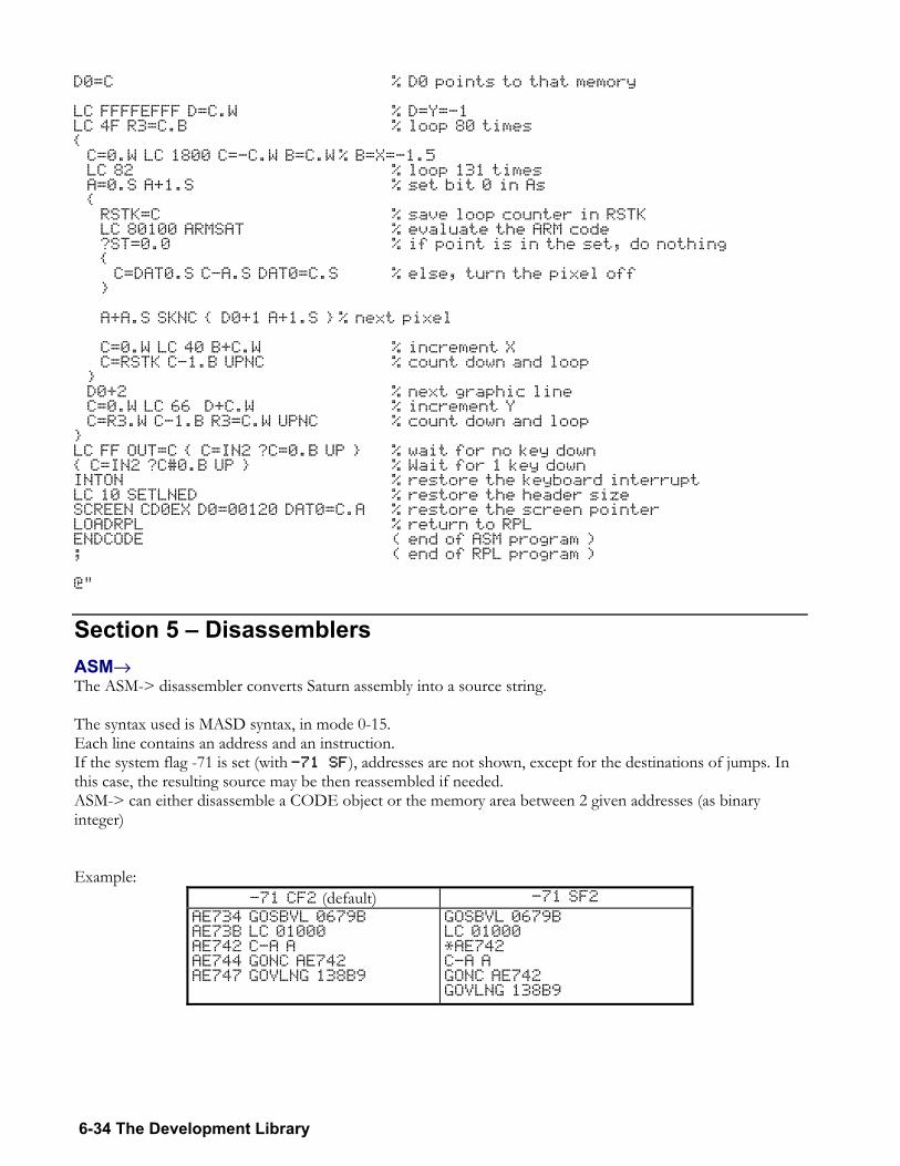
6-34 The Development Library
D0=C % D0 points to that memory LC FFFFEFFF D=C.W % D=Y=-1 LC 4F R3=C.B % loop 80 times C=0.W LC 1800 C=-C.W B=C.W % B=X=-1.5 LC 82 % loop 131 times A=0.S A+1.S % set bit 0 in As RSTK=C % save loop counter in RSTK LC 80100 ARMSAT % evaluate the ARM code ?ST=0.0 % if point is in the set, do nothing C=DAT0.S C-A.S DAT0=C.S % else, turn the pixel off A+A.S SKNC D0+1 A+1.S % next pixel C=0.W LC 40 B+C.W % increment X C=RSTK C-1.B UPNC % count down and loop D0+2 % next graphic line C=0.W LC 66 D+C.W % increment Y C=R3.W C-1.B R3=C.W UPNC % count down and loop LC FF OUT=C C=IN2 ?C=0.B UP % wait for no key down C=IN2 ?C#0.B UP % Wait for 1 key down INTON % restore the keyboard interrupt LC 10 SETLNED % restore the header size SCREEN CD0EX D0=00120 DAT0=C.A % restore the screen pointer LOADRPL % return to RPL ENDCODE ( end of ASM program ) ; ( end of RPL program ) @"
Section 5 Disassemblers ASM→ The ASM-> disassembler converts Saturn assembly into a source string. The syntax used is MASD syntax, in mode 0-15. Each line contains an address and an instruction. If the system flag -71 is set (with -71 SF), addresses are not shown, except for the destinations of jumps. In this case, the resulting source may be then reassembled if needed. ASM-> can either disassemble a CODE object or the memory area between 2 given addresses (as binary integer) Example:
-71 CF2 (default) -71 SF2
AE734 GOSBVL 0679B AE73B LC 01000 AE742 C-A A AE744 GONC AE742 AE747 GOVLNG 138B9
GOSBVL 0679B LC 01000 *AE742 C-A A GONC AE742 GOVLNG 138B9
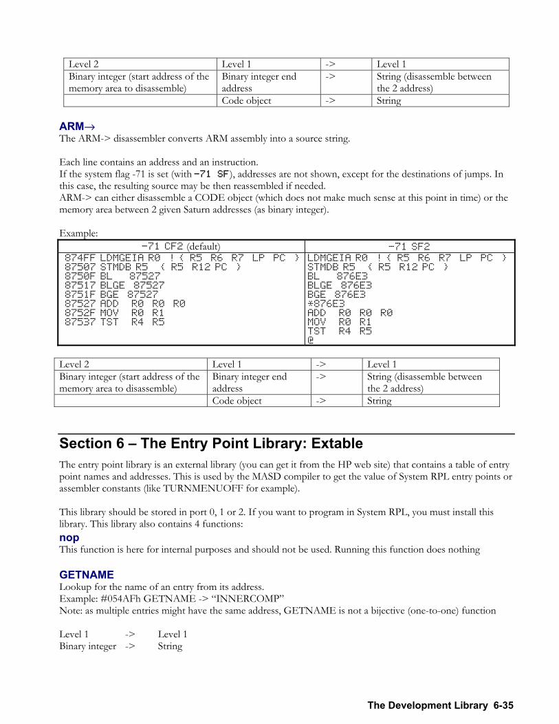
The Development Library 6-35
Level 2 Level 1 -> Level 1 Binary integer (start address of the memory area to disassemble)
Binary integer end address
-> String (disassemble between the 2 address)
Code object -> String ARM→ The ARM-> disassembler converts ARM assembly into a source string. Each line contains an address and an instruction. If the system flag -71 is set (with -71 SF), addresses are not shown, except for the destinations of jumps. In this case, the resulting source may be then reassembled if needed. ARM-> can either disassemble a CODE object (which does not make much sense at this point in time) or the memory area between 2 given Saturn addresses (as binary integer). Example:
-71 CF2 (default) -71 SF2 874FF LDMGEIA R0 ! R5 R6 R7 LP PC 87507 STMDB R5 R5 R12 PC 8750F BL 87527 87517 BLGE 87527 8751F BGE 87527 87527 ADD R0 R0 R0 8752F MOV R0 R1 87537 TST R4 R5
LDMGEIA R0 ! R5 R6 R7 LP PC STMDB R5 R5 R12 PC BL 876E3 BLGE 876E3 BGE 876E3 *876E3 ADD R0 R0 R0 MOV R0 R1 TST R4 R5 @
Level 2 Level 1 -> Level 1 Binary integer (start address of the memory area to disassemble)
Binary integer end address
-> String (disassemble between the 2 address)
Code object -> String
Section 6 The Entry Point Library: Extable The entry point library is an external library (you can get it from the HP web site) that contains a table of entry point names and addresses. This is used by the MASD compiler to get the value of System RPL entry points or assembler constants (like TURNMENUOFF for example). This library should be stored in port 0, 1 or 2. If you want to program in System RPL, you must install this library. This library also contains 4 functions: nop This function is here for internal purposes and should not be used. Running this function does nothing GETNAME Lookup for the name of an entry from its address. Example: #054AFh GETNAME -> INNERCOMP Note: as multiple entries might have the same address, GETNAME is not a bijective (one-to-one) function Level 1 -> Level 1 Binary integer -> String
6-36 The Development Library
GETADR Lookup for the address of an entry. Example: INNERCOMP GETADR -> #054Afh Level 1 -> Level 1 String -> Binary integer GETNAMES Find all the entry whose name starts with a specific string. Note: giving a null string as an input will return a list of all the entry points. Level 1 -> Level 1 String -> List of entry names.
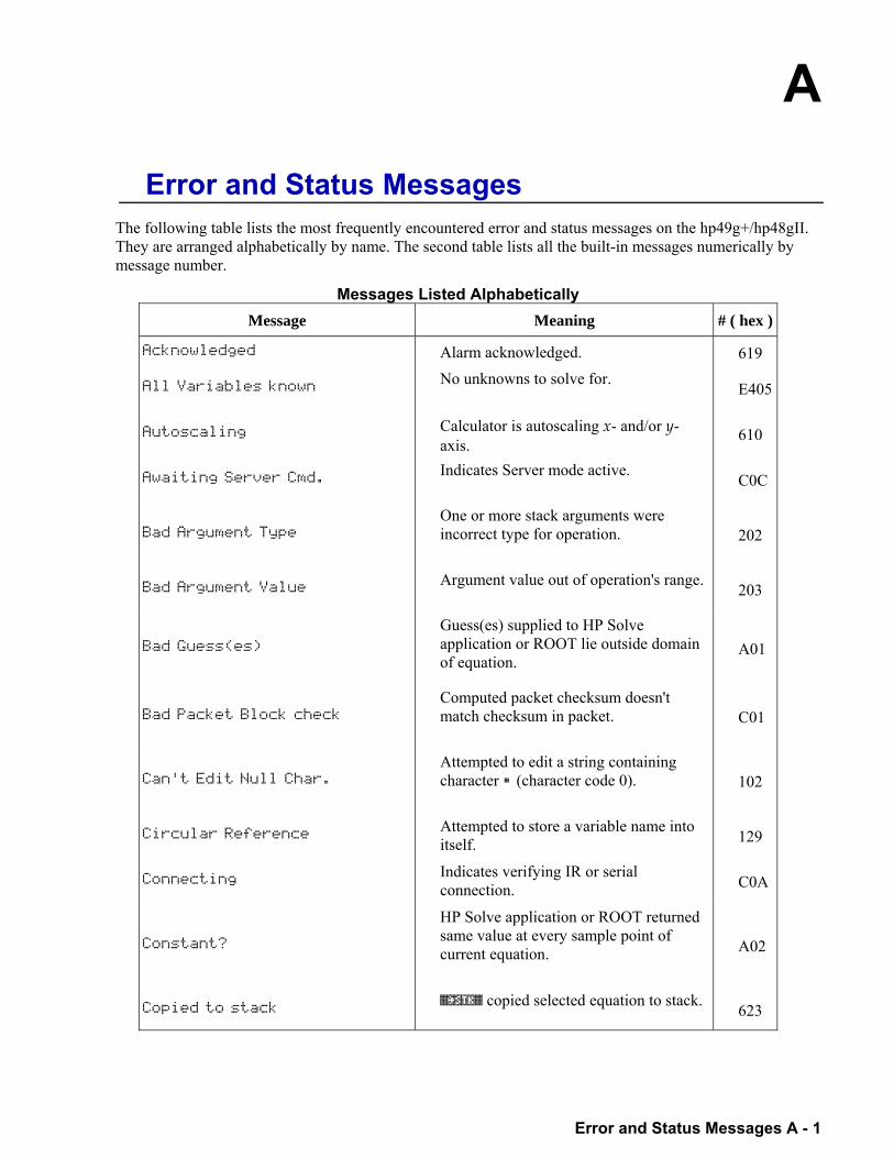
A
Error and Status Messages A - 1
7.Error and Status Messages The following table lists the most frequently encountered error and status messages on the hp49g+/hp48gII. They are arranged alphabetically by name. The second table lists all the built-in messages numerically by message number.
Messages Listed Alphabetically Message Meaning # ( hex )
Acknowledged Alarm acknowledged. 619
All Variables known No unknowns to solve for. E405
Autoscaling Calculator is autoscaling x- and/or y- axis.
610
Awaiting Server Cmd. Indicates Server mode active. C0C
Bad Argument Type One or more stack arguments were incorrect type for operation. 202
Bad Argument Value Argument value out of operation's range. 203
Bad Guess(es)
Guess(es) supplied to HP Solve application or ROOT lie outside domain of equation.
A01
Bad Packet Block check Computed packet checksum doesn't match checksum in packet. C01
Can't Edit Null Char. Attempted to edit a string containing character (character code 0). 102
Circular Reference Attempted to store a variable name into itself. 129
Connecting Indicates verifying IR or serial connection. C0A
Constant?
HP Solve application or ROOT returned same value at every sample point of current equation. A02
Copied to stack %²STK% copied selected equation to stack. 623
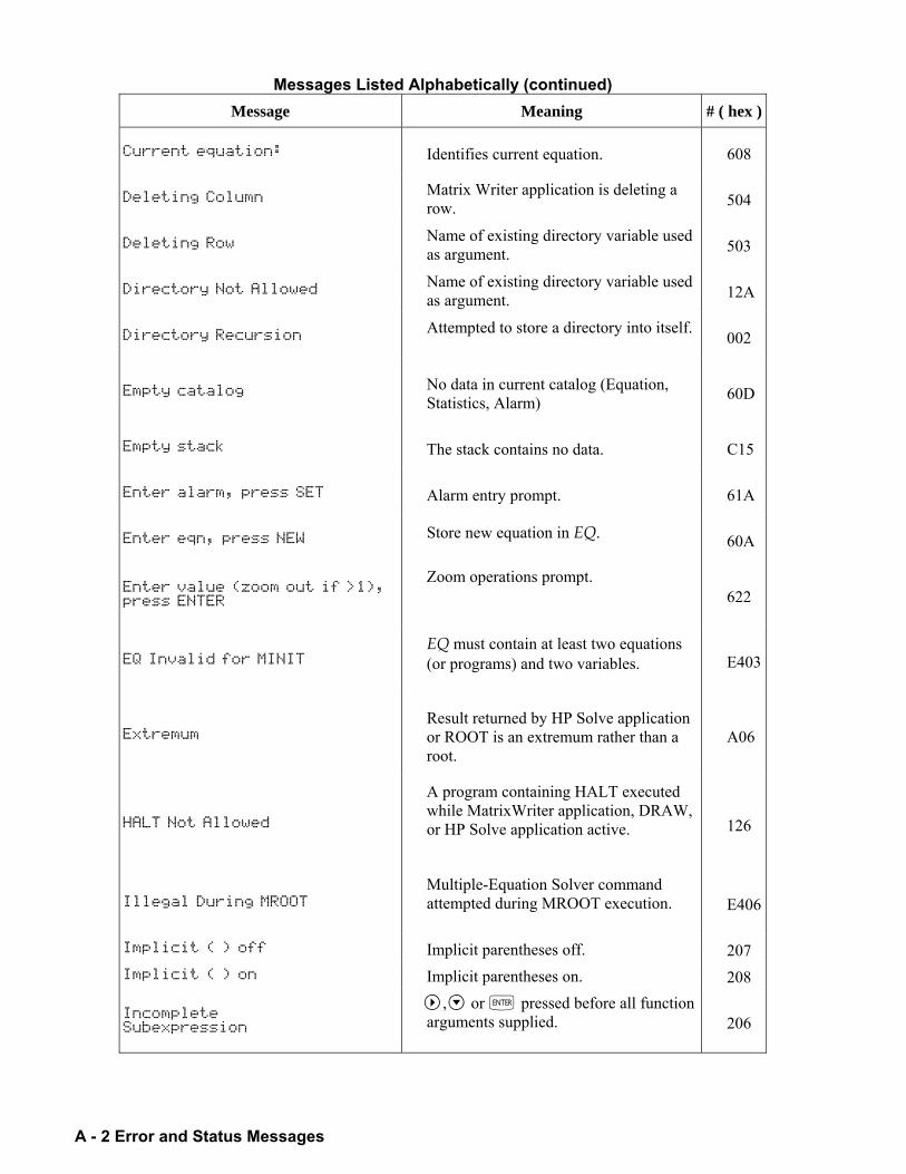
A - 2 Error and Status Messages
Messages Listed Alphabetically (continued) Message Meaning # ( hex )
Current equation: Identifies current equation. 608
Deleting Column Matrix Writer application is deleting a row. 504
Deleting Row Name of existing directory variable used as argument. 503
Directory Not Allowed Name of existing directory variable used as argument. 12A
Directory Recursion Attempted to store a directory into itself. 002
Empty catalog No data in current catalog (Equation, Statistics, Alarm) 60D
Empty stack The stack contains no data. C15
Enter alarm, press SET Alarm entry prompt. 61A
Enter eqn, press NEW Store new equation in EQ. 60A
Enter value (zoom out if >1), press ENTER
Zoom operations prompt. 622
EQ Invalid for MINIT EQ must contain at least two equations (or programs) and two variables. E403
Extremum Result returned by HP Solve application or ROOT is an extremum rather than a root.
A06
HALT Not Allowed
A program containing HALT executed while MatrixWriter application, DRAW, or HP Solve application active. 126
Illegal During MROOT Multiple-Equation Solver command attempted during MROOT execution. E406
Implicit ( ) off Implicit parentheses off. 207 Implicit ( ) on Implicit parentheses on. 208
Incomplete Subexpression
, or ` pressed before all function arguments supplied. 206
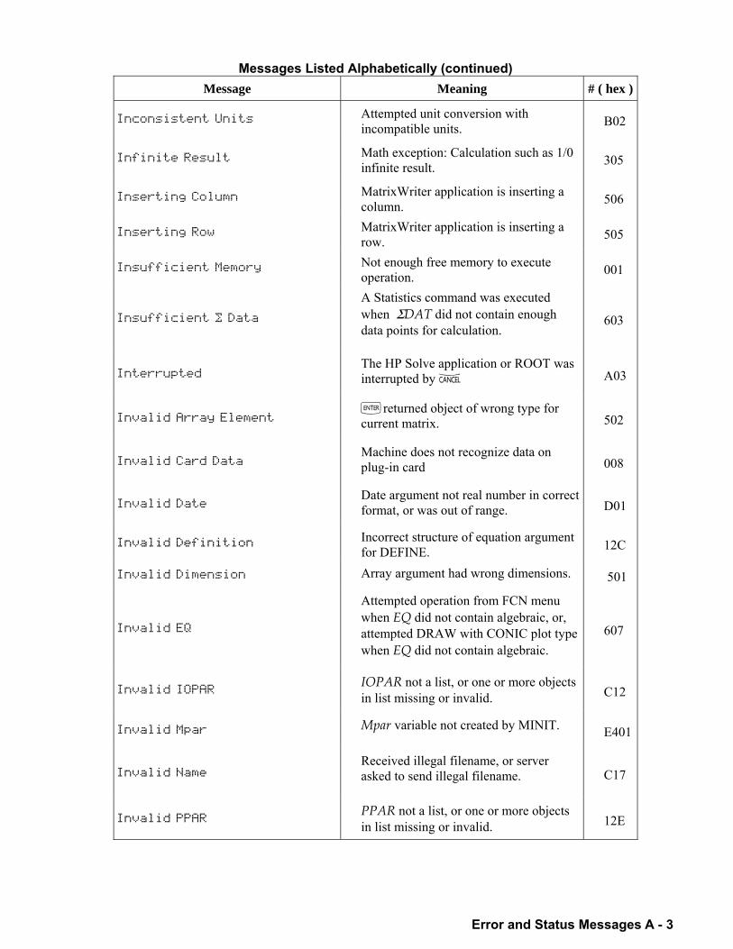
Error and Status Messages A - 3
Messages Listed Alphabetically (continued) Message Meaning # ( hex )
Inconsistent Units Attempted unit conversion with incompatible units. B02
Infinite Result Math exception: Calculation such as 1/0 infinite result. 305
Inserting Column MatrixWriter application is inserting a column. 506
Inserting Row MatrixWriter application is inserting a row. 505
Insufficient Memory Not enough free memory to execute operation. 001
Insufficient … Data
A Statistics command was executed when ΣDAT did not contain enough data points for calculation.
603
Interrupted The HP Solve application or ROOT was interrupted by − A03
Invalid Array Element `returned object of wrong type for current matrix. 502
Invalid Card Data Machine does not recognize data on plug-in card 008
Invalid Date Date argument not real number in correct format, or was out of range. D01
Invalid Definition Incorrect structure of equation argument for DEFINE. 12C
Invalid Dimension Array argument had wrong dimensions. 501
Invalid EQ
Attempted operation from FCN menu when EQ did not contain algebraic, or, attempted DRAW with CONIC plot type when EQ did not contain algebraic.
607
Invalid IOPAR IOPAR not a list, or one or more objects in list missing or invalid. C12
Invalid Mpar Mpar variable not created by MINIT. E401
Invalid Name Received illegal filename, or server asked to send illegal filename. C17
Invalid PPAR PPAR not a list, or one or more objects in list missing or invalid. 12E
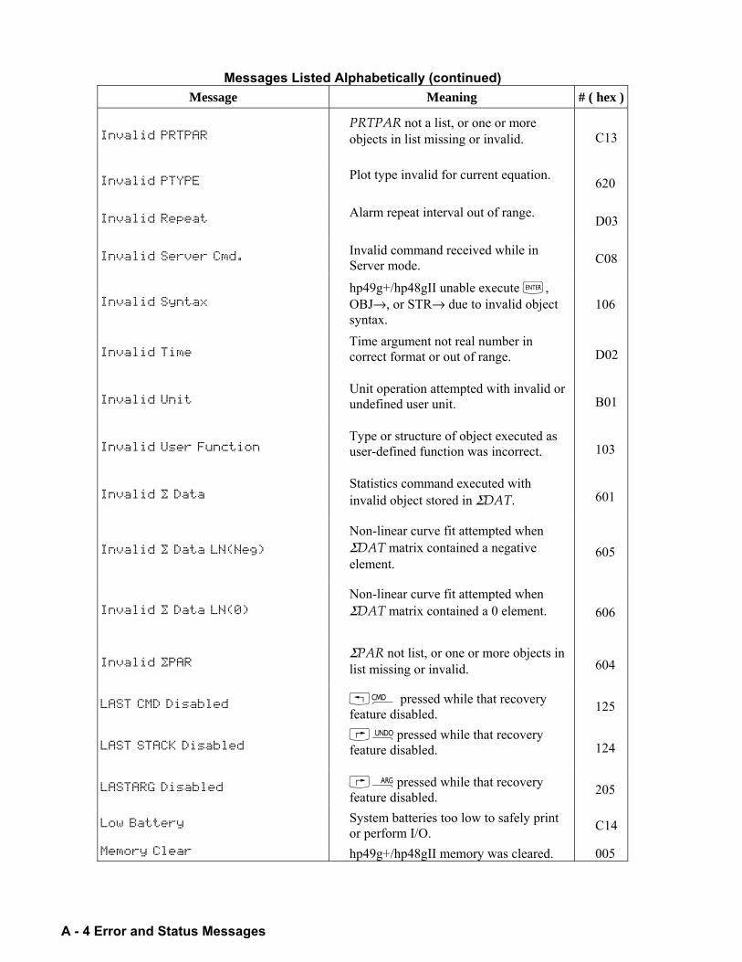
A - 4 Error and Status Messages
Messages Listed Alphabetically (continued) Message Meaning # ( hex )
Invalid PRTPAR PRTPAR not a list, or one or more objects in list missing or invalid. C13
Invalid PTYPE Plot type invalid for current equation. 620
Invalid Repeat Alarm repeat interval out of range. D03
Invalid Server Cmd. Invalid command received while in Server mode. C08
Invalid Syntax hp49g+/hp48gII unable execute `, OBJ→, or STR→ due to invalid object syntax.
106
Invalid Time Time argument not real number in correct format or out of range. D02
Invalid Unit Unit operation attempted with invalid or undefined user unit. B01
Invalid User Function Type or structure of object executed as user-defined function was incorrect. 103
Invalid … Data Statistics command executed with invalid object stored in ΣDAT. 601
Invalid … Data LN(Neg)
Non-linear curve fit attempted when ΣDAT matrix contained a negative element.
605
Invalid … Data LN(0)
Non-linear curve fit attempted when ΣDAT matrix contained a 0 element. 606
Invalid …PAR ΣPAR not list, or one or more objects in list missing or invalid. 604
LAST CMD Disabled ® pressed while that recovery feature disabled. 125
LAST STACK Disabled ¯pressed while that recovery feature disabled. 124
LASTARG Disabled Ëpressed while that recovery feature disabled. 205
Low Battery System batteries too low to safely print or perform I/O. C14
Memory Clear hp49g+/hp48gII memory was cleared. 005
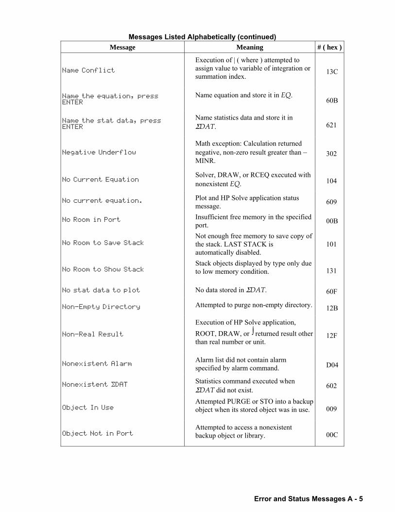
Error and Status Messages A - 5
Messages Listed Alphabetically (continued) Message Meaning # ( hex )
Name Conflict
Execution of | ( where ) attempted to assign value to variable of integration or summation index.
13C
Name the equation, press ENTER
Name equation and store it in EQ. 60B
Name the stat data, press ENTER
Name statistics data and store it in ΣDAT. 621
Negative Underflow
Math exception: Calculation returned negative, non-zero result greater than MINR.
302
No Current Equation Solver, DRAW, or RCEQ executed with nonexistent EQ. 104
No current equation. Plot and HP Solve application status message. 609
No Room in Port Insufficient free memory in the specified port. 00B
No Room to Save Stack Not enough free memory to save copy of the stack. LAST STACK is automatically disabled.
101
No Room to Show Stack Stack objects displayed by type only due to low memory condition. 131
No stat data to plot No data stored in ΣDAT. 60F
Non-Empty Directory Attempted to purge non-empty directory. 12B
Non-Real Result
Execution of HP Solve application, ROOT, DRAW, or ∫ returned result other than real number or unit.
12F
Nonexistent Alarm Alarm list did not contain alarm specified by alarm command. D04
Nonexistent …DAT Statistics command executed when ΣDAT did not exist. 602
Object In Use Attempted PURGE or STO into a backup object when its stored object was in use. 009
Object Not in Port Attempted to access a nonexistent backup object or library. 00C
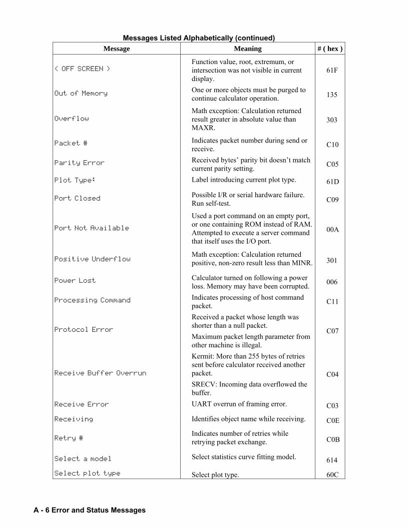
A - 6 Error and Status Messages
Messages Listed Alphabetically (continued) Message Meaning # ( hex )
( OFF SCREEN ) Function value, root, extremum, or intersection was not visible in current display.
61F
Out of Memory One or more objects must be purged to continue calculator operation. 135
Overflow Math exception: Calculation returned result greater in absolute value than MAXR.
303
Packet # Indicates packet number during send or receive. C10
Parity Error Received bytes parity bit doesnt match current parity setting. C05
Plot Type: Label introducing current plot type. 61D
Port Closed Possible I/R or serial hardware failure. Run self-test. C09
Port Not Available
Used a port command on an empty port, or one containing ROM instead of RAM. Attempted to execute a server command that itself uses the I/O port.
00A
Positive Underflow Math exception: Calculation returned positive, non-zero result less than MINR. 301
Power Lost Calculator turned on following a power loss. Memory may have been corrupted. 006
Processing Command Indicates processing of host command packet. C11
Protocol Error
Received a packet whose length was shorter than a null packet. Maximum packet length parameter from other machine is illegal.
C07
Receive Buffer Overrun
Kermit: More than 255 bytes of retries sent before calculator received another packet. SRECV: Incoming data overflowed the buffer.
C04
Receive Error UART overrun of framing error. C03
Receiving Identifies object name while receiving. C0E
Retry # Indicates number of retries while retrying packet exchange. C0B
Select a model Select statistics curve fitting model. 614
Select plot type Select plot type. 60C
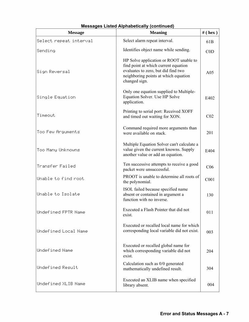
Error and Status Messages A - 7
Messages Listed Alphabetically (continued) Message Meaning # ( hex )
Select repeat interval Select alarm repeat interval. 61B
Sending Identifies object name while sending. C0D
Sign Reversal
HP Solve application or ROOT unable to find point at which current equation evaluates to zero, but did find two neighboring points at which equation changed sign.
A05
Single Equation
Only one equation supplied to Multiple-Equation Solver. Use HP Solve application.
E402
Timeout Printing to serial port: Received XOFF and timed out waiting for XON. C02
Too Few Arguments Command required more arguments than were available on stack. 201
Too Many Unknowns
Multiple Equation Solver can't calculate a value given the current knowns. Supply another value or add an equation.
E404
Transfer Failed Ten successive attempts to receive a good packet were unsuccessful. C06
Unable to find root PROOT is unable to determine all roots of the polynomial. C001
Unable to Isolate ISOL failed because specified name absent or contained in argument a function with no inverse.
130
Undefined FPTR Name Executed a Flash Pointer that did not exist. 011
Undefined Local Name
Executed or recalled local name for which corresponding local variable did not exist. 003
Undefined Name Executed or recalled global name for which corresponding variable did not exist.
204
Undefined Result Calculation such as 0/0 generated mathematically undefined result. 304
Undefined XLIB Name Executed an XLIB name when specified library absent. 004
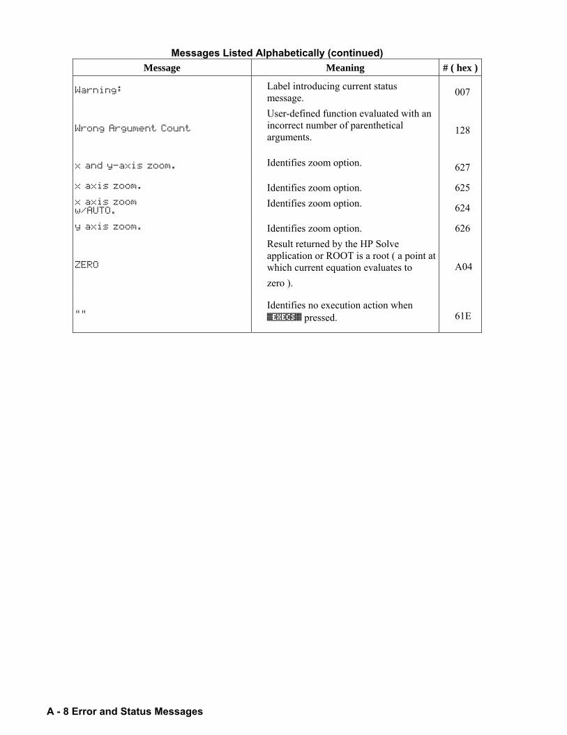
A - 8 Error and Status Messages
Messages Listed Alphabetically (continued) Message Meaning # ( hex )
Warning: Label introducing current status message. 007
Wrong Argument Count
User-defined function evaluated with an incorrect number of parenthetical arguments.
128
x and y-axis zoom. Identifies zoom option. 627
x axis zoom. Identifies zoom option. 625 x axis zoom w/AUTO.
Identifies zoom option. 624
y axis zoom. Identifies zoom option. 626
ZERO
Result returned by the HP Solve application or ROOT is a root ( a point at which current equation evaluates to zero ).
A04
"" Identifies no execution action when %EXECS% pressed. 61E
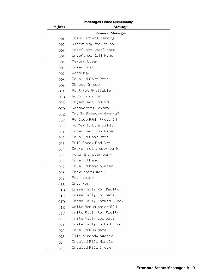
Error and Status Messages A - 9
Messages Listed Numerically # (hex) Message
General Messages001 Insufficient Memory
002 Directory Recursion
003 Undefined Local Name
004 Undefined XLIB Name
005 Memory Clear
006 Power Lost
007 Warning:
008 Invalid Card Data
009 Object In use
00A Port Not Available
00B No Room in Port
00C Object Not in Port
00D Recovering Memory
00E Try To Recover Memory?
00F Replace RAM, Press ON
010 No Mem To Config All
011 Undefined FPTR Name
012 Invalid Bank Data
013 Full Check Bad Crc
014 Cmprs: not a user bank
015 No or 2 system bank
016 Invalid bank
017 Invalid bank number
018 Inexisting pack
019 Pack twice
01A Ins. Mem.
01B Erase Fail, Rom faulty
01C Erase Fail, Low bats
01D Erase Fail, Locked Block
01E Write Adr outside ROM
01F Write Fail, Rom Faulty
020 Write Fail, Low bats
021 Write Fail, Locked Block
022 Invalid DOS Name
023 File already opened
024 Invalid File Handle
025 Invalid File Index
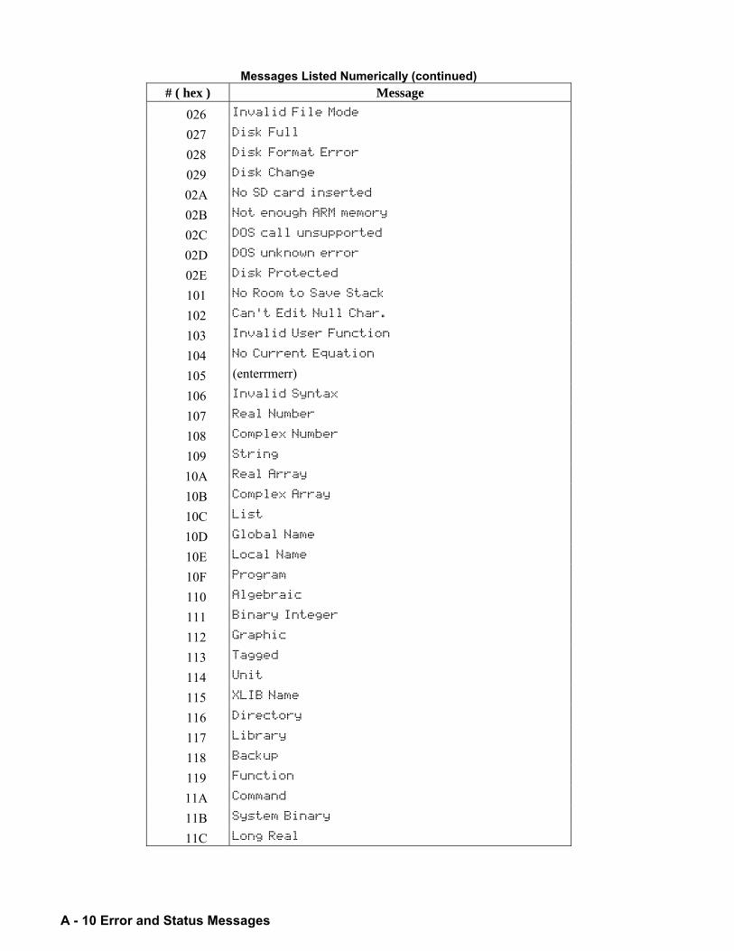
A - 10 Error and Status Messages
Messages Listed Numerically (continued) # ( hex ) Message
026 Invalid File Mode
027 Disk Full
028 Disk Format Error
029 Disk Change
02A No SD card inserted
02B Not enough ARM memory
02C DOS call unsupported
02D DOS unknown error
02E Disk Protected
101 No Room to Save Stack
102 Can't Edit Null Char.
103 Invalid User Function
104 No Current Equation
105 (enterrmerr)
106 Invalid Syntax
107 Real Number
108 Complex Number
109 String
10A Real Array
10B Complex Array
10C List
10D Global Name
10E Local Name
10F Program
110 Algebraic
111 Binary Integer
112 Graphic
113 Tagged
114 Unit
115 XLIB Name
116 Directory
117 Library
118 Backup
119 Function
11A Command
11B System Binary
11C Long Real
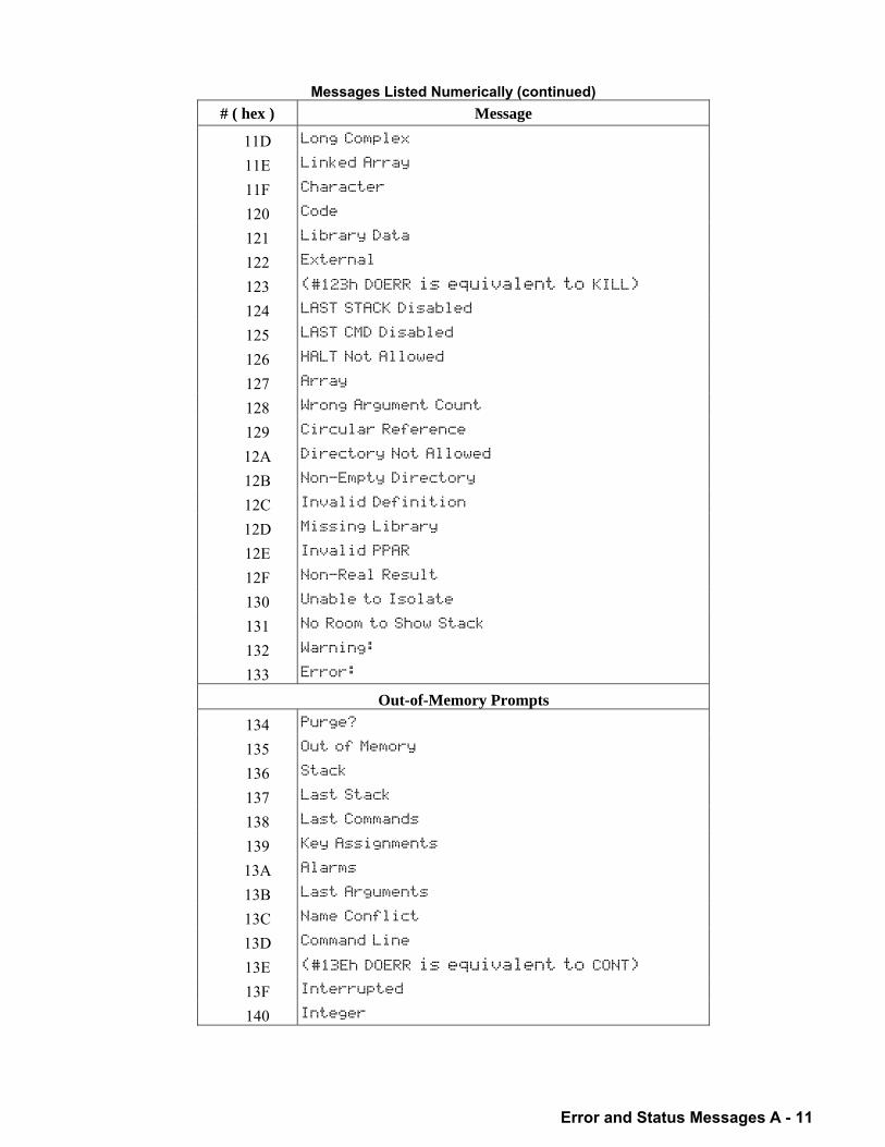
Error and Status Messages A - 11
Messages Listed Numerically (continued) # ( hex ) Message
11D Long Complex
11E Linked Array
11F Character
120 Code
121 Library Data
122 External
123 (#123h DOERR is equivalent to KILL)
124 LAST STACK Disabled
125 LAST CMD Disabled
126 HALT Not Allowed
127 Array
128 Wrong Argument Count
129 Circular Reference
12A Directory Not Allowed
12B Non-Empty Directory
12C Invalid Definition
12D Missing Library
12E Invalid PPAR
12F Non-Real Result
130 Unable to Isolate
131 No Room to Show Stack
132 Warning:
133 Error:
Out-of-Memory Prompts 134 Purge?
135 Out of Memory
136 Stack
137 Last Stack
138 Last Commands
139 Key Assignments
13A Alarms
13B Last Arguments
13C Name Conflict
13D Command Line
13E (#13Eh DOERR is equivalent to CONT)
13F Interrupted
140 Integer
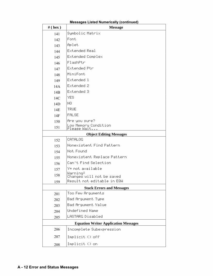
A - 12 Error and Status Messages
Messages Listed Numerically (continued) # ( hex ) Message
141 Symbolic Matrix
142 Font
143 Aplet
144 Extended Real
145 Extended Complex
146 FlashPtr
147 Extended Ptr
148 MiniFont
149 Extended 1
14A Extended 2
14B Extended 3
14C YES
14D NO
14E TRUE
14F FALSE
150 Are you sure?
151 Low Memory Condition Please Wait...
Object Editing Messages 152 CATALOG
153 Nonexistent Find Pattern
154 Not Found
155 Nonexistent Replace Pattern
156 Can't Find Selection
157 Y= not available
158 Warning: Changes will not be saved
159 Result not editable in EQW
Stack Errors and Messages 201 Too Few Arguments
202 Bad Argument Type
203 Bad Argument Value
204 Undefined Name
205 LASTARG Disabled
Equation Writer Application Messages 206 Incomplete Subexpression
207 Implicit () off
208 Implicit () on
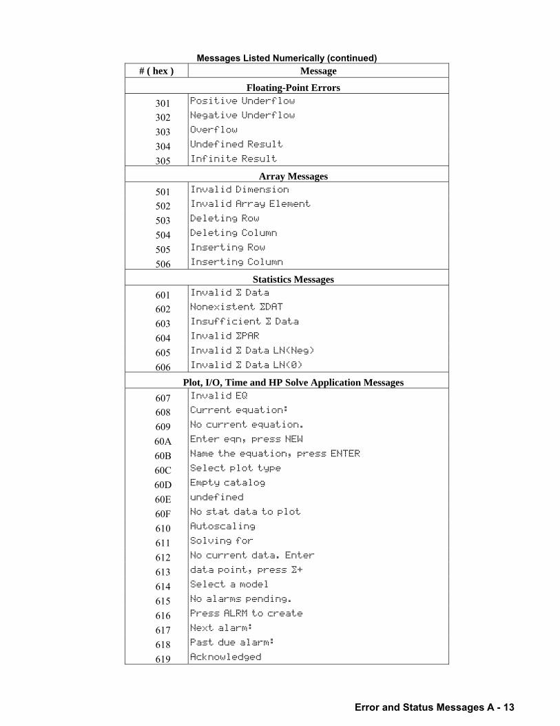
Error and Status Messages A - 13
Messages Listed Numerically (continued) # ( hex ) Message
Floating-Point Errors 301 Positive Underflow
302 Negative Underflow
303 Overflow
304 Undefined Result
305 Infinite Result
Array Messages 501 Invalid Dimension
502 Invalid Array Element
503 Deleting Row
504 Deleting Column
505 Inserting Row
506 Inserting Column
Statistics Messages 601 Invalid … Data
602 Nonexistent …DAT
603 Insufficient … Data
604 Invalid …PAR
605 Invalid … Data LN(Neg)
606 Invalid … Data LN(0)
Plot, I/O, Time and HP Solve Application Messages 607 Invalid EQ
608 Current equation:
609 No current equation.
60A Enter eqn, press NEW
60B Name the equation, press ENTER
60C Select plot type
60D Empty catalog
60E undefined
60F No stat data to plot
610 Autoscaling
611 Solving for
612 No current data. Enter
613 data point, press …+
614 Select a model
615 No alarms pending.
616 Press ALRM to create
617 Next alarm:
618 Past due alarm:
619 Acknowledged
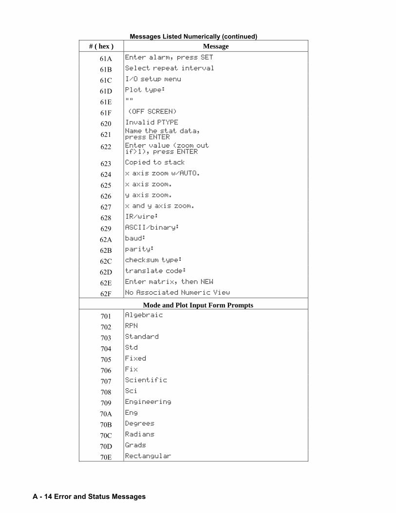
A - 14 Error and Status Messages
Messages Listed Numerically (continued) # ( hex ) Message
61A Enter alarm, press SET
61B Select repeat interval
61C I/O setup menu
61D Plot type:
61E ""
61F (OFF SCREEN)
620 Invalid PTYPE
621 Name the stat data, press ENTER
622 Enter value (zoom out if>1), press ENTER
623 Copied to stack
624 x axis zoom w/AUTO.
625 x axis zoom.
626 y axis zoom.
627 x and y axis zoom.
628 IR/wire:
629 ASCII/binary:
62A baud:
62B parity:
62C checksum type:
62D translate code:
62E Enter matrix, then NEW
62F No Associated Numeric View
Mode and Plot Input Form Prompts 701 Algebraic
702 RPN
703 Standard
704 Std
705 Fixed
706 Fix
707 Scientific
708 Sci
709 Engineering
70A Eng
70B Degrees
70C Radians
70D Grads
70E Rectangular
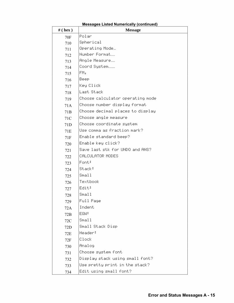
Error and Status Messages A - 15
Messages Listed Numerically (continued) # ( hex ) Message
70F Polar
710 Spherical
711 Operating ModeÏ.
712 Number FormatÏÏ.
713 Angle MeasureÏÏ.
714 Coord SystemÏÏÏÏ
715 FM,
716 Beep
717 Key Click
718 Last Stack
719 Choose calculator operating mode
71A Choose number display format
71B Choose decimal places to display
71C Choose angle measure
71D Choose coordinate system
71E Use comma as fraction mark?
71F Enable standard beep?
720 Enable key click?
721 Save last stk for UNDO and ANS?
722 CALCULATOR MODES
723 Font:
724 Stack:
725 Small
726 Textbook
727 Edit:
728 Small
729 Full Page
72A Indent
72B EQW:
72C Small
72D Small Stack Disp
72E Header:
72F Clock
730 Analog
731 Choose system font
732 Display stack using small font?
733 Use pretty print in the stack?
734 Edit using small font?
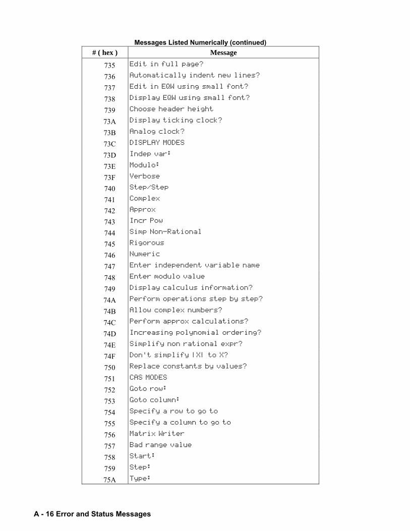
A - 16 Error and Status Messages
Messages Listed Numerically (continued) # ( hex ) Message
735 Edit in full page?
736 Automatically indent new lines?
737 Edit in EQW using small font?
738 Display EQW using small font?
739 Choose header height
73A Display ticking clock?
73B Analog clock?
73C DISPLAY MODES
73D Indep var:
73E Modulo:
73F Verbose
740 Step/Step
741 Complex
742 Approx
743 Incr Pow
744 Simp Non-Rational
745 Rigorous
746 Numeric
747 Enter independent variable name
748 Enter modulo value
749 Display calculus information?
74A Perform operations step by step?
74B Allow complex numbers?
74C Perform approx calculations?
74D Increasing polynomial ordering?
74E Simplify non rational expr?
74F Don't simplify |X| to X?
750 Replace constants by values?
751 CAS MODES
752 Goto row:
753 Goto column:
754 Specify a row to go to
755 Specify a column to go to
756 Matrix Writer
757 Bad range value
758 Start:
759 Step:
75A Type:
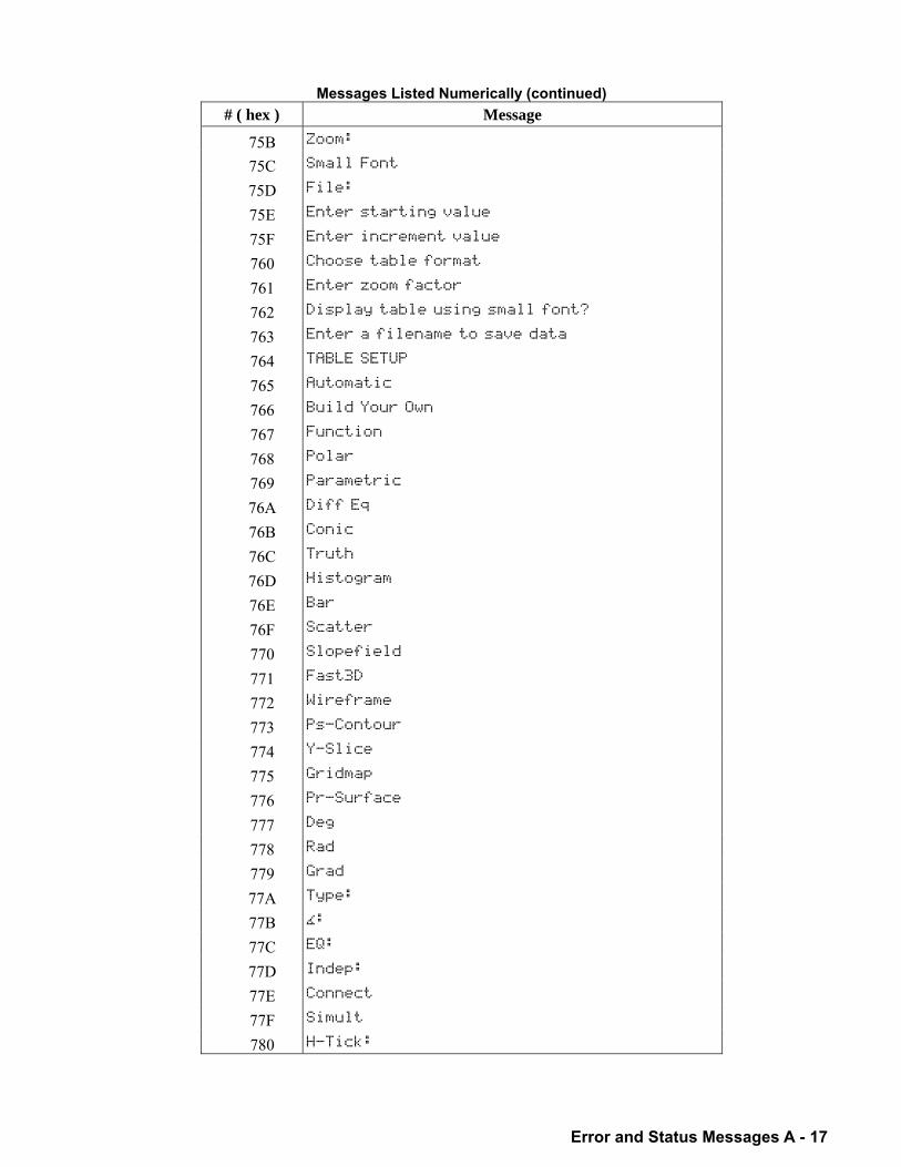
Error and Status Messages A - 17
Messages Listed Numerically (continued) # ( hex ) Message
75B Zoom:
75C Small Font
75D File:
75E Enter starting value
75F Enter increment value
760 Choose table format
761 Enter zoom factor
762 Display table using small font?
763 Enter a filename to save data
764 TABLE SETUP
765 Automatic
766 Build Your Own
767 Function
768 Polar
769 Parametric
76A Diff Eq
76B Conic
76C Truth
76D Histogram
76E Bar
76F Scatter
770 Slopefield
771 Fast3D
772 Wireframe
773 Ps-Contour
774 Y-Slice
775 Gridmap
776 Pr-Surface
777 Deg
778 Rad
779 Grad
77A Type:
77B :
77C EQ:
77D Indep:
77E Connect
77F Simult
780 H-Tick:
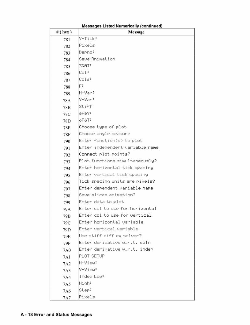
A - 18 Error and Status Messages
Messages Listed Numerically (continued) # ( hex ) Message
781 V-Tick:
782 Pixels
783 Depnd:
784 Save Animation
785 …DAT:
786 Col:
787 Cols:
788 F:
789 H-Var:
78A V-Var:
78B Stiff
78C ˆFˆY:
78D ˆFˆT:
78E Choose type of plot
78F Choose angle measure
790 Enter function(s) to plot
791 Enter independent variable name
792 Connect plot points?
793 Plot functions simultaneously?
794 Enter horizontal tick spacing
795 Enter vertical tick spacing
796 Tick spacing units are pixels?
797 Enter dependent variable name
798 Save slices animation?
799 Enter data to plot
79A Enter col to use for horizontal
79B Enter col to use for vertical
79C Enter horizontal variable
79D Enter vertical variable
79E Use stiff diff eq solver?
79F Enter derivative w.r.t. soln
7A0 Enter derivative w.r.t. indep
7A1 PLOT SETUP
7A2 H-View:
7A3 V-View:
7A4 Indep Low:
7A5 High:
7A6 Step:
7A7 Pixels
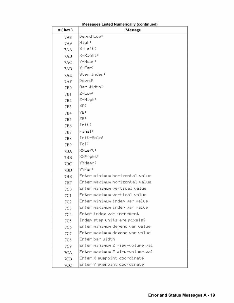
Error and Status Messages A - 19
Messages Listed Numerically (continued) # ( hex ) Message
7A8 Depnd Low:
7A9 High:
7AA X-Left:
7AB X-Right:
7AC Y-Near:
7AD Y-Far:
7AE Step Indep:
7AF Depnd:
7B0 Bar Width:
7B1 Z-Low:
7B2 Z-High:
7B3 XE:
7B4 YE:
7B5 ZE:
7B6 Init:
7B7 Final:
7B8 Init-Soln:
7B9 Tol:
7BA XXLeft:
7BB XXRight:
7BC YYNear:
7BD YYFar:
7BE Enter minimum horizontal value
7BF Enter maximum horizontal value
7C0 Enter minimum vertical value
7C1 Enter maximum vertical value
7C2 Enter minimum indep var value
7C3 Enter maximum indep var value
7C4 Enter indep var increment
7C5 Indep step units are pixels?
7C6 Enter minimum depend var value
7C7 Enter maximum depend var value
7C8 Enter bar width
7C9 Enter minimum Z view-volume val
7CA Enter maximum Z view-volume val
7CB Enter X eyepoint coordinate
7CC Enter Y eyepoint coordinate
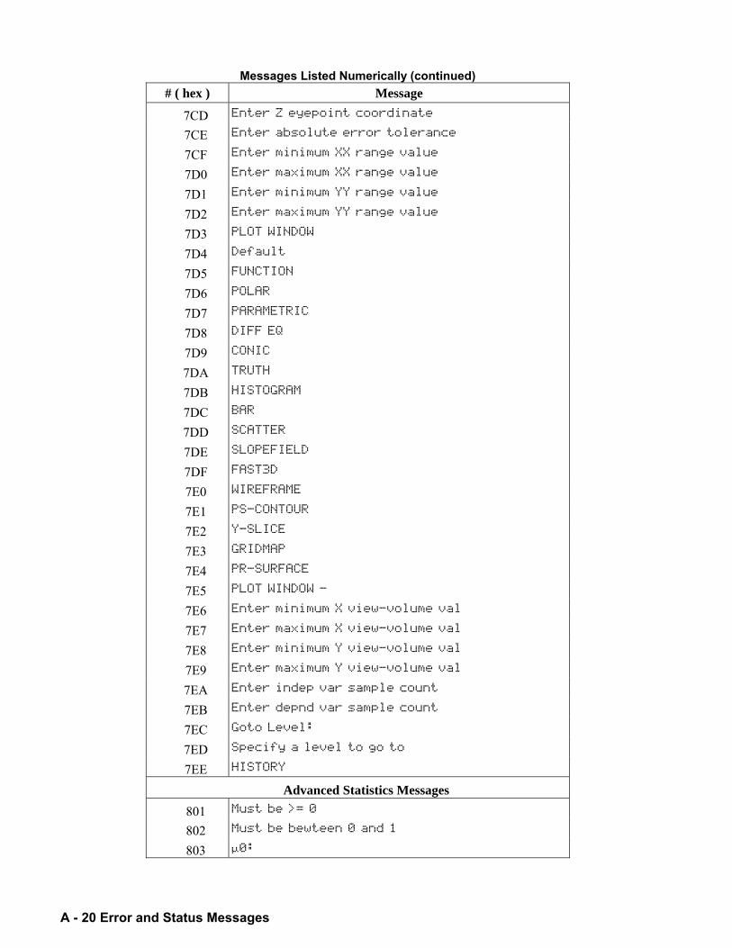
A - 20 Error and Status Messages
Messages Listed Numerically (continued) # ( hex ) Message
7CD Enter Z eyepoint coordinate
7CE Enter absolute error tolerance
7CF Enter minimum XX range value
7D0 Enter maximum XX range value
7D1 Enter minimum YY range value
7D2 Enter maximum YY range value
7D3 PLOT WINDOW
7D4 Default
7D5 FUNCTION
7D6 POLAR
7D7 PARAMETRIC
7D8 DIFF EQ
7D9 CONIC
7DA TRUTH
7DB HISTOGRAM
7DC BAR
7DD SCATTER
7DE SLOPEFIELD
7DF FAST3D
7E0 WIREFRAME
7E1 PS-CONTOUR
7E2 Y-SLICE
7E3 GRIDMAP
7E4 PR-SURFACE
7E5 PLOT WINDOW -
7E6 Enter minimum X view-volume val
7E7 Enter maximum X view-volume val
7E8 Enter minimum Y view-volume val
7E9 Enter maximum Y view-volume val
7EA Enter indep var sample count
7EB Enter depnd var sample count
7EC Goto Level:
7ED Specify a level to go to
7EE HISTORY
Advanced Statistics Messages 801 Must be >= 0
802 Must be bewteen 0 and 1
803 µ0:
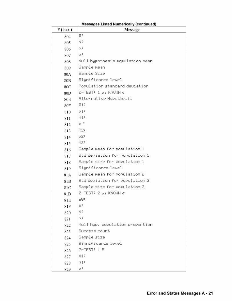
Error and Status Messages A - 21
Messages Listed Numerically (continued) # ( hex ) Message
804 :
805 N:
806 Œ:
807 ˜:
808 Null hypothesis population mean
809 Sample mean
80A Sample Size
80B Significance level
80C Population standard deviation
80D Z-TEST: 1 µ, KNOWN ˜
80E Alternative Hypothesis
80F 1:
810 ˜1:
811 N1:
812 Π:
813 2:
814 ˜2:
815 N2:
816 Sample mean for population 1
817 Std deviation for population 1
818 Sample size for population 1
819 Significance level
81A Sample mean for population 2
81B Std deviation for population 2
81C Sample size for population 2
81D Z-TEST: 2 µ, KNOWN ˜
81E ‡0:
81F x:
820 N:
821 Œ:
822 Null hyp. population proportion
823 Success count
824 Sample size
825 Significance level
826 Z-TEST: 1 P
827 X1:
828 N1:
829 Œ:
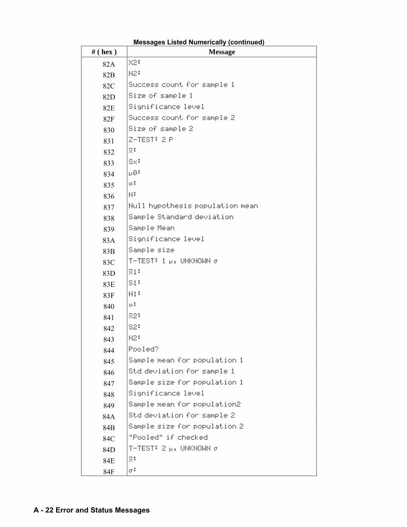
A - 22 Error and Status Messages
Messages Listed Numerically (continued) # ( hex ) Message
82A X2:
82B N2:
82C Success count for sample 1
82D Size of sample 1
82E Significance level
82F Success count for sample 2
830 Size of sample 2
831 Z-TEST: 2 P
832 :
833 Sx:
834 µ0:
835 Œ:
836 N:
837 Null hypothesis population mean
838 Sample Standard deviation
839 Sample Mean
83A Significance level
83B Sample size
83C T-TEST: 1 µ, UNKNOWN ˜
83D 1:
83E S1:
83F N1:
840 Œ:
841 2:
842 S2:
843 N2:
844 Pooled?
845 Sample mean for population 1
846 Std deviation for sample 1
847 Sample size for population 1
848 Significance level
849 Sample mean for population2
84A Std deviation for sample 2
84B Sample size for population 2
84C "Pooled" if checked
84D T-TEST: 2 µ, UNKNOWN ˜
84E :
84F ˜:
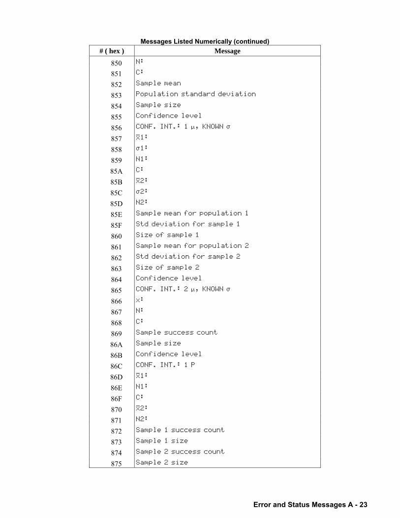
Error and Status Messages A - 23
Messages Listed Numerically (continued) # ( hex ) Message
850 N:
851 C:
852 Sample mean
853 Population standard deviation
854 Sample size
855 Confidence level
856 CONF. INT.: 1 µ, KNOWN ˜
857 1:
858 ˜1:
859 N1:
85A C:
85B 2:
85C ˜2:
85D N2:
85E Sample mean for population 1
85F Std deviation for sample 1
860 Size of sample 1
861 Sample mean for population 2
862 Std deviation for sample 2
863 Size of sample 2
864 Confidence level
865 CONF. INT.: 2 µ, KNOWN ˜
866 x:
867 N:
868 C:
869 Sample success count
86A Sample size
86B Confidence level
86C CONF. INT.: 1 P
86D 1:
86E N1:
86F C:
870 2:
871 N2:
872 Sample 1 success count
873 Sample 1 size
874 Sample 2 success count
875 Sample 2 size
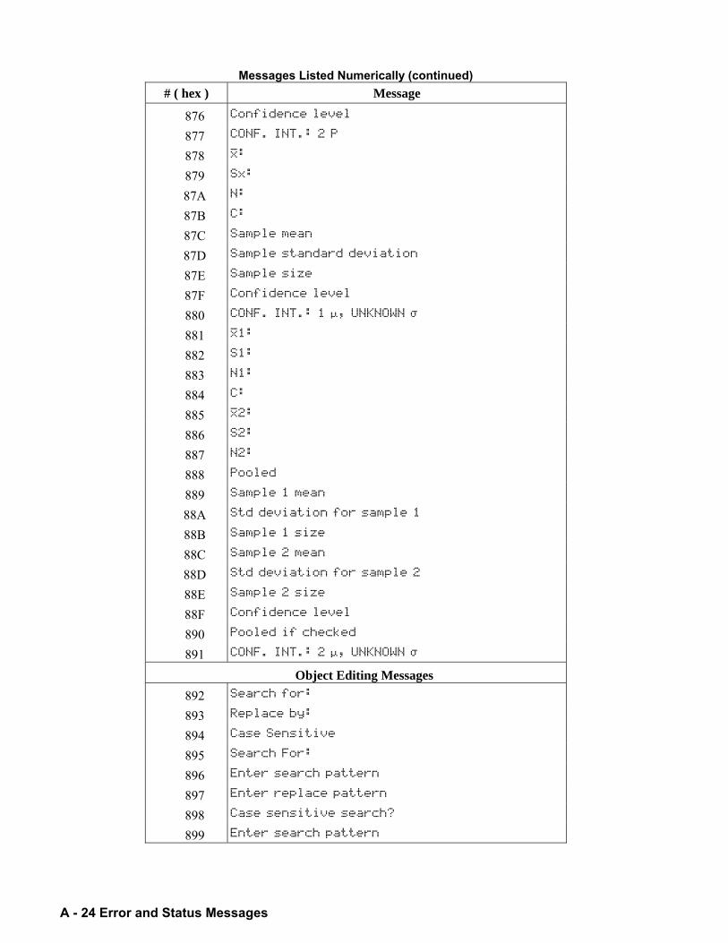
A - 24 Error and Status Messages
Messages Listed Numerically (continued) # ( hex ) Message
876 Confidence level
877 CONF. INT.: 2 P
878 :
879 Sx:
87A N:
87B C:
87C Sample mean
87D Sample standard deviation
87E Sample size
87F Confidence level
880 CONF. INT.: 1 µ, UNKNOWN ˜
881 1:
882 S1:
883 N1:
884 C:
885 2:
886 S2:
887 N2:
888 Pooled
889 Sample 1 mean
88A Std deviation for sample 1
88B Sample 1 size
88C Sample 2 mean
88D Std deviation for sample 2
88E Sample 2 size
88F Confidence level
890 Pooled if checked
891 CONF. INT.: 2 µ, UNKNOWN ˜
Object Editing Messages 892 Search for:
893 Replace by:
894 Case Sensitive
895 Search For:
896 Enter search pattern
897 Enter replace pattern
898 Case sensitive search?
899 Enter search pattern
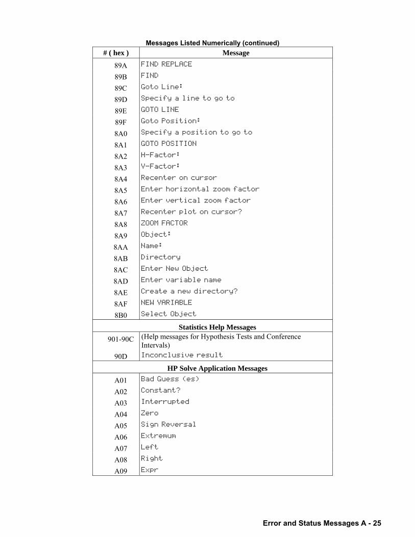
Error and Status Messages A - 25
Messages Listed Numerically (continued) # ( hex ) Message
89A FIND REPLACE
89B FIND
89C Goto Line:
89D Specify a line to go to
89E GOTO LINE
89F Goto Position:
8A0 Specify a position to go to
8A1 GOTO POSITION
8A2 H-Factor:
8A3 V-Factor:
8A4 Recenter on cursor
8A5 Enter horizontal zoom factor
8A6 Enter vertical zoom factor
8A7 Recenter plot on cursor?
8A8 ZOOM FACTOR
8A9 Object:
8AA Name:
8AB Directory
8AC Enter New Object
8AD Enter variable name
8AE Create a new directory?
8AF NEW VARIABLE
8B0 Select Object
Statistics Help Messages 901-90C (Help messages for Hypothesis Tests and Conference
Intervals) 90D Inconclusive result
HP Solve Application Messages A01 Bad Guess (es)
A02 Constant?
A03 Interrupted
A04 Zero
A05 Sign Reversal
A06 Extremum
A07 Left
A08 Right
A09 Expr
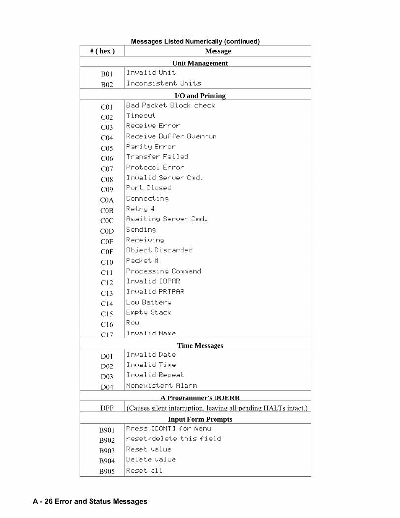
A - 26 Error and Status Messages
Messages Listed Numerically (continued) # ( hex ) Message
Unit ManagementB01 Invalid Unit
B02 Inconsistent Units
I/O and Printing C01 Bad Packet Block check
C02 Timeout
C03 Receive Error
C04 Receive Buffer Overrun
C05 Parity Error
C06 Transfer Failed
C07 Protocol Error
C08 Invalid Server Cmd.
C09 Port Closed
C0A Connecting
C0B Retry #
C0C Awaiting Server Cmd.
C0D Sending
C0E Receiving
C0F Object Discarded
C10 Packet #
C11 Processing Command
C12 Invalid IOPAR
C13 Invalid PRTPAR
C14 Low Battery
C15 Empty Stack
C16 Row
C17 Invalid Name
Time MessagesD01 Invalid Date
D02 Invalid Time
D03 Invalid Repeat
D04 Nonexistent Alarm
A Programmer's DOERR DFF (Causes silent interruption, leaving all pending HALTs intact.)
Input Form Prompts B901 Press [CONT] for menu
B902 reset/delete this field
B903 Reset value
B904 Delete value
B905 Reset all
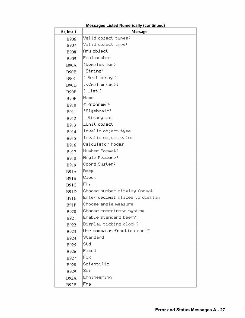
Error and Status Messages A - 27
Messages Listed Numerically (continued) # ( hex ) Message
B906 Valid object types:
B907 Valid object type:
B908 Any object
B909 Real number
B90A (Complex num)
B90B "String"
B90C [ Real array ]
B90D [(Cmpl array)]
B90E List
B90F Name
B910 « Program »
B911 'Algebraic'
B912 # Binary int
B913 _Unit object
B914 Invalid object type
B915 Invalid object value
B916 Calculator Modes
B917 Number Format:
B918 Angle Measure:
B919 Coord System:
B91A Beep
B91B Clock
B91C FM,
B91D Choose number display format
B91E Enter decimal places to display
B91F Choose angle measure
B920 Choose coordinate system
B921 Enable standard beep?
B922 Display ticking clock?
B923 Use comma as fraction mark?
B924 Standard
B925 Std
B926 Fixed
B927 Fix
B928 Scientific
B929 Sci
B92A Engineering
B92B Eng
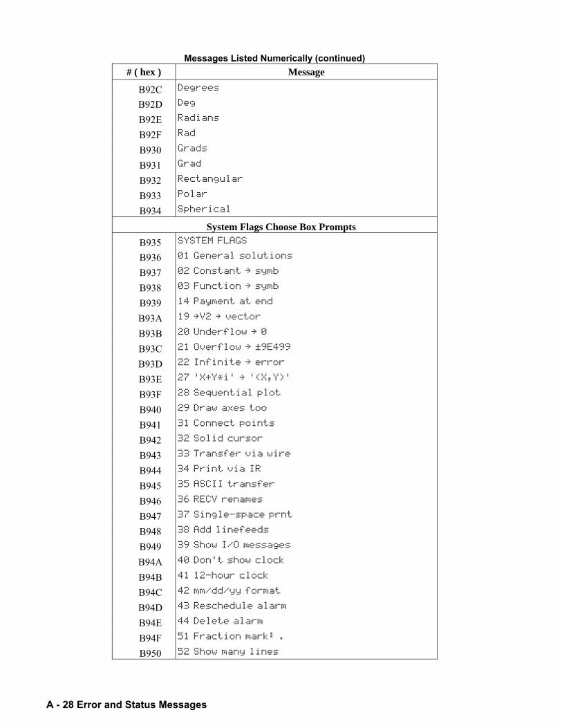
A - 28 Error and Status Messages
Messages Listed Numerically (continued) # ( hex ) Message
B92C Degrees
B92D Deg
B92E Radians
B92F Rad
B930 Grads
B931 Grad
B932 Rectangular
B933 Polar
B934 Spherical
System Flags Choose Box Prompts B935 SYSTEM FLAGS
B936 01 General solutions
B937 02 Constant symb
B938 03 Function symb
B939 14 Payment at end
B93A 19 V2 vector
B93B 20 Underflow 0
B93C 21 Overflow ±9E499
B93D 22 Infinite error
B93E 27 'X+Y*i' '(X,Y)'
B93F 28 Sequential plot
B940 29 Draw axes too
B941 31 Connect points
B942 32 Solid cursor
B943 33 Transfer via wire
B944 34 Print via IR
B945 35 ASCII transfer
B946 36 RECV renames
B947 37 Single-space prnt
B948 38 Add linefeeds
B949 39 Show I/O messages
B94A 40 Don't show clock
B94B 41 12-hour clock
B94C 42 mm/dd/yy format
B94D 43 Reschedule alarm
B94E 44 Delete alarm
B94F 51 Fraction mark: .
B950 52 Show many lines
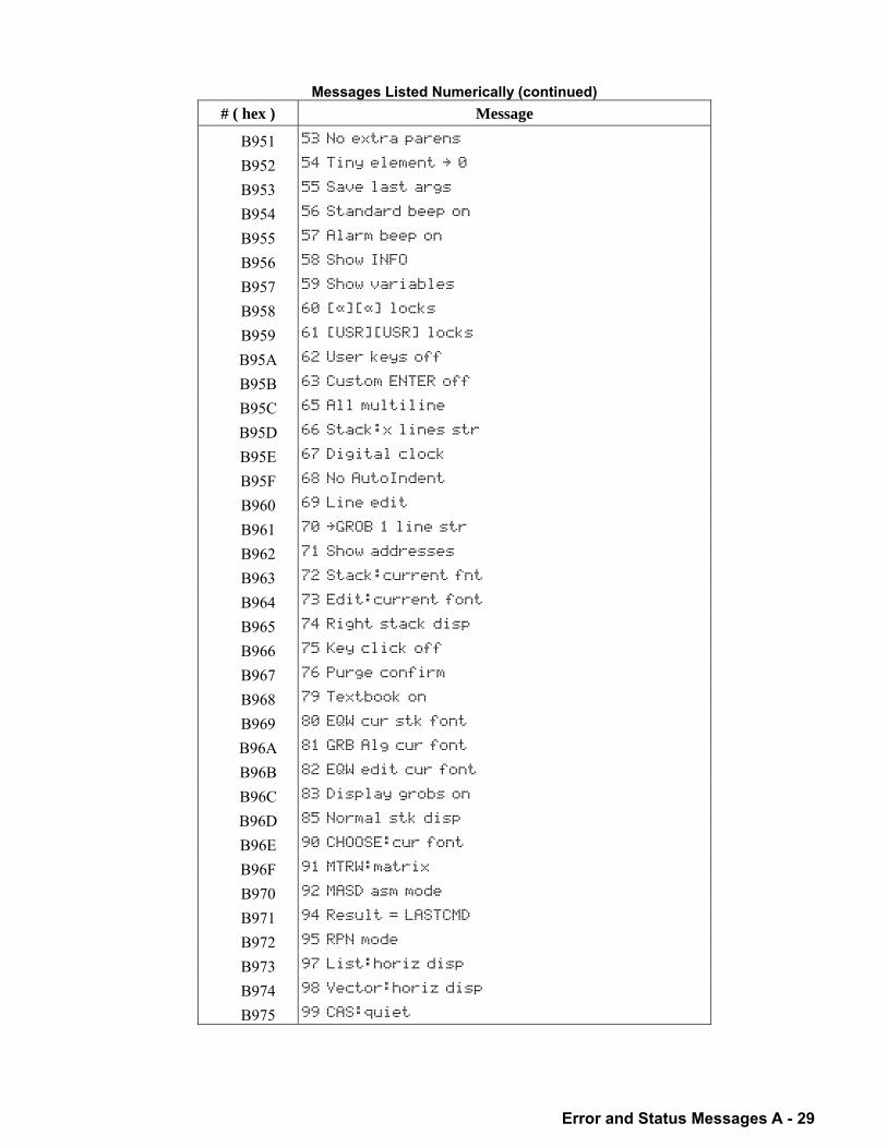
Error and Status Messages A - 29
Messages Listed Numerically (continued) # ( hex ) Message
B951 53 No extra parens
B952 54 Tiny element 0
B953 55 Save last args
B954 56 Standard beep on
B955 57 Alarm beep on
B956 58 Show INFO
B957 59 Show variables
B958 60 [Œ][Œ] locks
B959 61 [USR][USR] locks
B95A 62 User keys off
B95B 63 Custom ENTER off
B95C 65 All multiline
B95D 66 Stack:x lines str
B95E 67 Digital clock
B95F 68 No AutoIndent
B960 69 Line edit
B961 70 GROB 1 line str
B962 71 Show addresses
B963 72 Stack:current fnt
B964 73 Edit:current font
B965 74 Right stack disp
B966 75 Key click off
B967 76 Purge confirm
B968 79 Textbook on
B969 80 EQW cur stk font
B96A 81 GRB Alg cur font
B96B 82 EQW edit cur font
B96C 83 Display grobs on
B96D 85 Normal stk disp
B96E 90 CHOOSE:cur font
B96F 91 MTRW:matrix
B970 92 MASD asm mode
B971 94 Result = LASTCMD
B972 95 RPN mode
B973 97 List:horiz disp
B974 98 Vector:horiz disp
B975 99 CAS:quiet
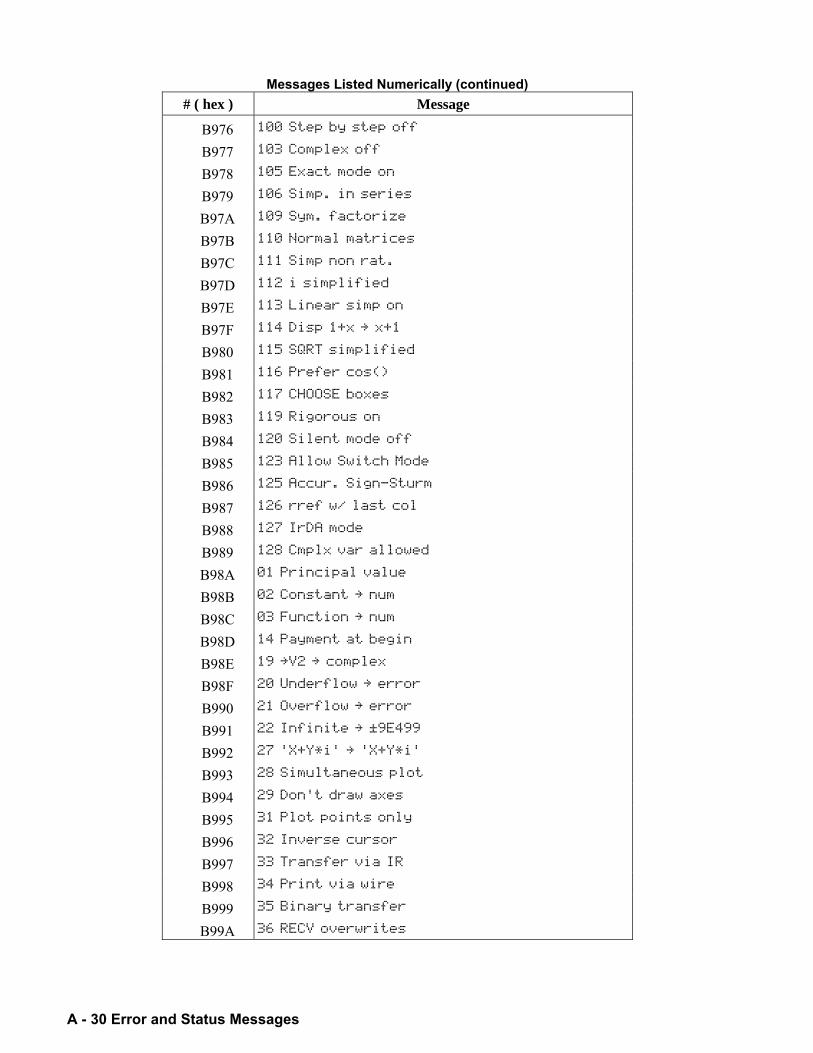
A - 30 Error and Status Messages
Messages Listed Numerically (continued) # ( hex ) Message
B976 100 Step by step off
B977 103 Complex off
B978 105 Exact mode on
B979 106 Simp. in series
B97A 109 Sym. factorize
B97B 110 Normal matrices
B97C 111 Simp non rat.
B97D 112 i simplified
B97E 113 Linear simp on
B97F 114 Disp 1+x x+1
B980 115 SQRT simplified
B981 116 Prefer cos()
B982 117 CHOOSE boxes
B983 119 Rigorous on
B984 120 Silent mode off
B985 123 Allow Switch Mode
B986 125 Accur. Sign-Sturm
B987 126 rref w/ last col
B988 127 IrDA mode
B989 128 Cmplx var allowed
B98A 01 Principal value
B98B 02 Constant num
B98C 03 Function num
B98D 14 Payment at begin
B98E 19 V2 complex
B98F 20 Underflow error
B990 21 Overflow error
B991 22 Infinite ±9E499
B992 27 'X+Y*i' 'X+Y*i'
B993 28 Simultaneous plot
B994 29 Don't draw axes
B995 31 Plot points only
B996 32 Inverse cursor
B997 33 Transfer via IR
B998 34 Print via wire
B999 35 Binary transfer
B99A 36 RECV overwrites
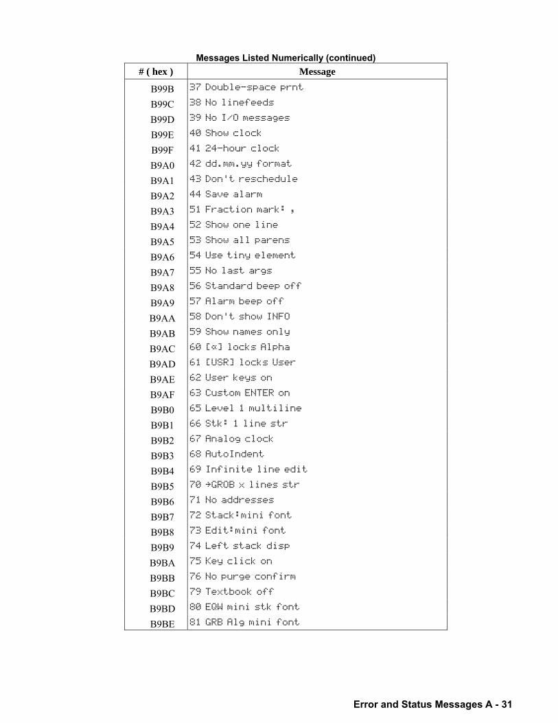
Error and Status Messages A - 31
Messages Listed Numerically (continued) # ( hex ) Message
B99B 37 Double-space prnt
B99C 38 No linefeeds
B99D 39 No I/O messages
B99E 40 Show clock
B99F 41 24-hour clock
B9A0 42 dd.mm.yy format
B9A1 43 Don't reschedule
B9A2 44 Save alarm
B9A3 51 Fraction mark: ,
B9A4 52 Show one line
B9A5 53 Show all parens
B9A6 54 Use tiny element
B9A7 55 No last args
B9A8 56 Standard beep off
B9A9 57 Alarm beep off
B9AA 58 Don't show INFO
B9AB 59 Show names only
B9AC 60 [Œ] locks Alpha
B9AD 61 [USR] locks User
B9AE 62 User keys on
B9AF 63 Custom ENTER on
B9B0 65 Level 1 multiline
B9B1 66 Stk: 1 line str
B9B2 67 Analog clock
B9B3 68 AutoIndent
B9B4 69 Infinite line edit
B9B5 70 GROB x lines str
B9B6 71 No addresses
B9B7 72 Stack:mini font
B9B8 73 Edit:mini font
B9B9 74 Left stack disp
B9BA 75 Key click on
B9BB 76 No purge confirm
B9BC 79 Textbook off
B9BD 80 EQW mini stk font
B9BE 81 GRB Alg mini font
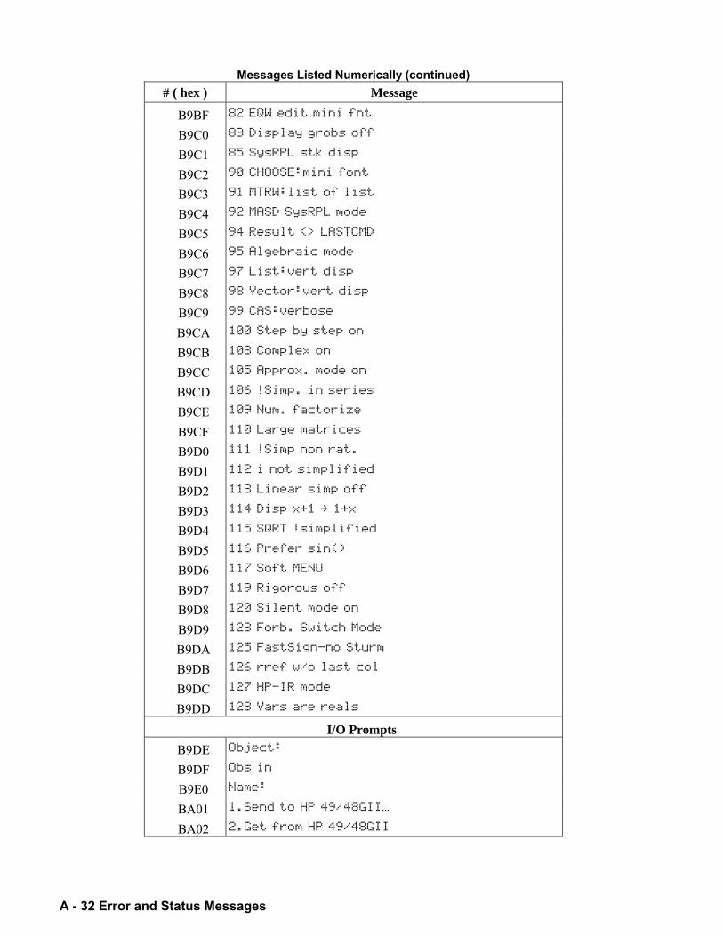
A - 32 Error and Status Messages
Messages Listed Numerically (continued) # ( hex ) Message
B9BF 82 EQW edit mini fnt
B9C0 83 Display grobs off
B9C1 85 SysRPL stk disp
B9C2 90 CHOOSE:mini font
B9C3 91 MTRW:list of list
B9C4 92 MASD SysRPL mode
B9C5 94 Result <> LASTCMD
B9C6 95 Algebraic mode
B9C7 97 List:vert disp
B9C8 98 Vector:vert disp
B9C9 99 CAS:verbose
B9CA 100 Step by step on
B9CB 103 Complex on
B9CC 105 Approx. mode on
B9CD 106 !Simp. in series
B9CE 109 Num. factorize
B9CF 110 Large matrices
B9D0 111 !Simp non rat.
B9D1 112 i not simplified
B9D2 113 Linear simp off
B9D3 114 Disp x+1 1+x
B9D4 115 SQRT !simplified
B9D5 116 Prefer sin()
B9D6 117 Soft MENU
B9D7 119 Rigorous off
B9D8 120 Silent mode on
B9D9 123 Forb. Switch Mode
B9DA 125 FastSign-no Sturm
B9DB 126 rref w/o last col
B9DC 127 HP-IR mode
B9DD 128 Vars are reals
I/O Prompts B9DE Object:
B9DF Obs in
B9E0 Name:
BA01 1.Send to HP 49/48GIIÏ.
BA02 2.Get from HP 49/48GII
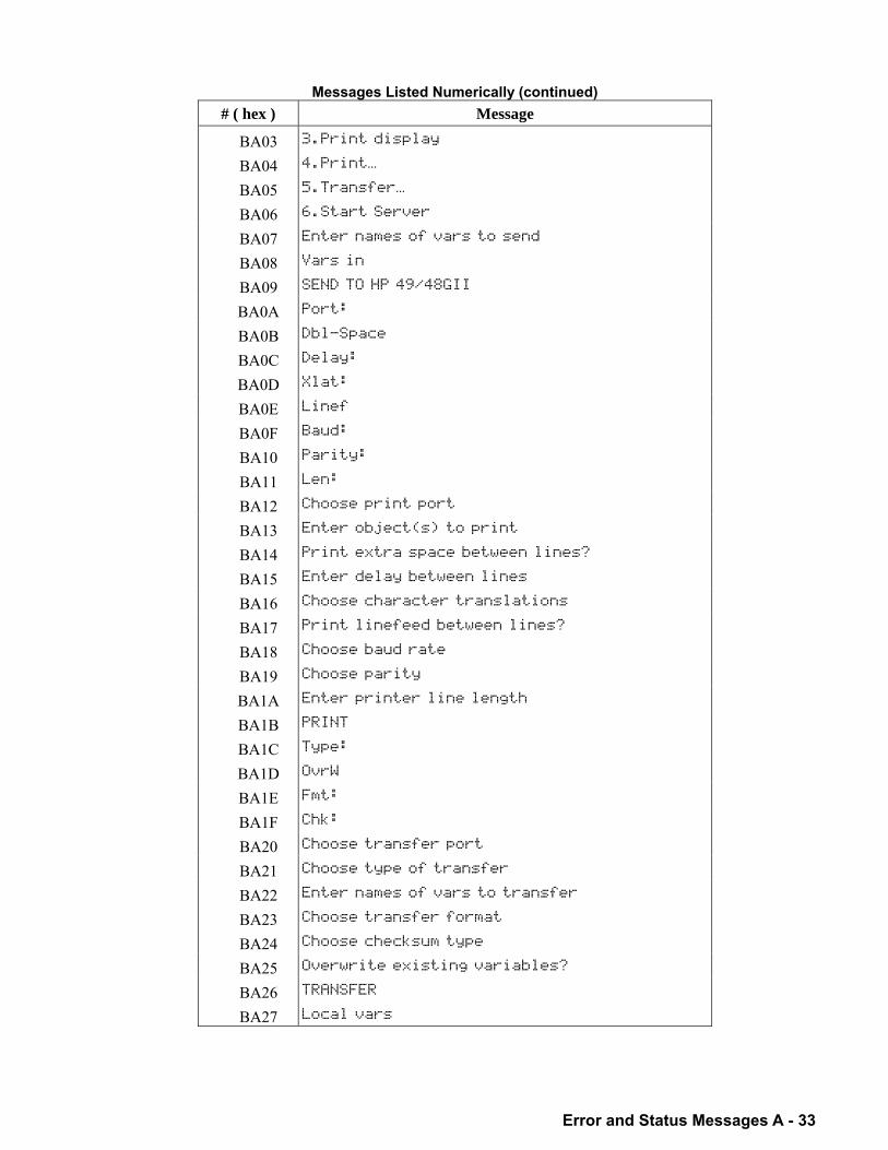
Error and Status Messages A - 33
Messages Listed Numerically (continued) # ( hex ) Message
BA03 3.Print display
BA04 4.PrintÏ.
BA05 5.TransferÏ.
BA06 6.Start Server
BA07 Enter names of vars to send
BA08 Vars in
BA09 SEND TO HP 49/48GII
BA0A Port:
BA0B Dbl-Space
BA0C Delay:
BA0D Xlat:
BA0E Linef
BA0F Baud:
BA10 Parity:
BA11 Len:
BA12 Choose print port
BA13 Enter object(s) to print
BA14 Print extra space between lines?
BA15 Enter delay between lines
BA16 Choose character translations
BA17 Print linefeed between lines?
BA18 Choose baud rate
BA19 Choose parity
BA1A Enter printer line length
BA1B PRINT
BA1C Type:
BA1D OvrW
BA1E Fmt:
BA1F Chk:
BA20 Choose transfer port
BA21 Choose type of transfer
BA22 Enter names of vars to transfer
BA23 Choose transfer format
BA24 Choose checksum type
BA25 Overwrite existing variables?
BA26 TRANSFER
BA27 Local vars
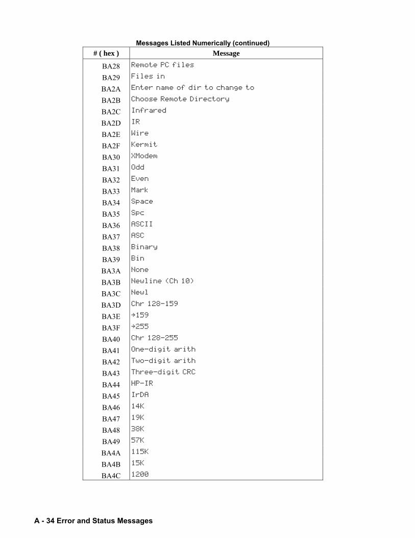
A - 34 Error and Status Messages
Messages Listed Numerically (continued) # ( hex ) Message
BA28 Remote PC files
BA29 Files in
BA2A Enter name of dir to change to
BA2B Choose Remote Directory
BA2C Infrared
BA2D IR
BA2E Wire
BA2F Kermit
BA30 XModem
BA31 Odd
BA32 Even
BA33 Mark
BA34 Space
BA35 Spc
BA36 ASCII
BA37 ASC
BA38 Binary
BA39 Bin
BA3A None
BA3B Newline (Ch 10)
BA3C Newl
BA3D Chr 128-159
BA3E 159
BA3F 255
BA40 Chr 128-255
BA41 One-digit arith
BA42 Two-digit arith
BA43 Three-digit CRC
BA44 HP-IR
BA45 IrDA
BA46 14K
BA47 19K
BA48 38K
BA49 57K
BA4A 115K
BA4B 15K
BA4C 1200
Error and Status Messages A - 35
Messages Listed Numerically (continued) # ( hex ) Message
BA4D 2400
BA4E 4800
BA4F 9600
Statistics Prompts BB01 1.Single-varÏ.
BB02 2.FrequenciesÏ.
BB03 3.Fit dataÏ.
BB04 4.Summary statsÏ.
BB05 SINGLE-VARIABLE STATISTICS
BB06 …DAT:
BB07 Type:
BB08 Mean
BB09 Std Dev
BB0A Variance
BB0B Total
BB0C Maximum
BB0D Minimum
BB0E Enter statistical data
BB0F Enter variable column
BB10 Choose statistics type
BB11 Calculate mean?
BB12 Calculate standard deviation?
BB13 Calculate variance?
BB14 Calculate column total?
BB15 Calculate column maximum?
BB16 Calculate column minimum?
BB17 Sample
BB18 Population
BB19 FREQUENCIES
BB1A X-Min:
BB1B Bin Count:
BB1C Bin Width:
BB1D Enter minimum first bin X value
BB1E Enter number of bins
BB1F Enter bin width
BB20 FIT DATA
BB21 X-Col:
A - 36 Error and Status Messages
Messages Listed Numerically (continued) # ( hex ) Message
BB22 Y-Col:
BB23 Model:
BB24 Enter indep column number
BB25 Enter dependent column number
BB26 Choose statistical model
BB27 Correlation
BB28 Covariance
BB29 PREDICT VALUES
BB2A Y:
BB2B Enter indep value or press PRED
BB2C Enter dep value or press PRED
BB2D SUMMARY STATISTICS
BB2E Calculate:
BB2F …X
BB30 …Y
BB31 …X2
BB32 …Y2
BB33 …XY
BB34 N…
BB35 Calculate sum of X column?
BB36 Calculate sum of Y column?
BB37 Calculate sum of squares of X?
BB38 Calculate sum of squares of Y?
BB39 Calculate sum of products?
BB3A Calculate number of data points?
BB3B Linear Fit
BB3C Logarithmic Fit
BB3D Exponential Fit
BB3E Power Fit
BB3F Best Fit
BB40 5.Hypoth. testsÏ.
BB41 6.Conf. intervalÏ.
Time and Alarm Prompts BC01 1.Browse alarmsÏ.
BC02 2.Set alarmÏ.
BC03 3.Set time, dateÏ.
BC04 SET ALARM
Error and Status Messages A - 37
Messages Listed Numerically (continued) # ( hex ) Message
BC05 Message:
BC06 Time:
BC07 Date:
BC08 Repeat:
BC09 Enter "message" or « action »
BC0A Enter hour
BC0B Enter minute
BC0C Enter second
BC0D Choose AM, PM, or 24-hour time
BC0E Enter month
BC0F Enter day
BC10 Enter year
BC11 Enter alarm repeat multiple
BC12 Enter alarm repeat unit
BC13 SET TIME AND DATE
BC14 Choose date display format
BC15 Monday
BC16 Tuesday
BC17 Wednesday
BC18 Thursday
BC19 Friday
BC1A Saturday
BC1B Sunday
BC1C None
BC1D AM
BC1E PM
BC1F 24-hour time
BC20 24-hr
BC21 1 January
BC22 2 February
BC23 3 March
BC24 4 April
BC25 5 May
BC26 6 June
BC27 7 July
BC28 8 August
BC29 9 September
A - 38 Error and Status Messages
Messages Listed Numerically (continued) # ( hex ) Message
BC2A 10 October
BC2B 11 November
BC2C 12 December
BC2D Week
BC2E Day
BC2F Hour
BC30 Minute
BC31 Second
BC32 Weeks
BC33 Days
BC34 Hours
BC35 Minutes
BC36 Seconds
BC37 Month/Day/Year
BC38 M/D/Y
BC39 Day.Month.Year
BC3A D.M.Y
BC3B ALARMS
Symbolic Application Prompts BD01 1.IntegrateÏ.
BD02 2.DifferentiateÏ.
BD03 3.Taylor polyÏ.
BD04 4.Isolate varÏ.
BD05 5.Solve quadÏ.
BD06 6.Manip exprÏ.
BD07 INTEGRATE
BD08 Expr:
BD09 Var:
BD0A Result:
BD0B Enter expression
BD0C Enter variable name
BD0D Enter lower limit
BD0E Enter upper limit
BD0F Choose result type
BD10 Choose disp format for accuracy
BD11 DIFFERENTIATE
BD12 Value:
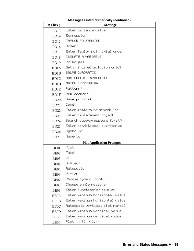
Error and Status Messages A - 39
Messages Listed Numerically (continued) # ( hex ) Message
BD13 Enter variable value
BD14 Expression
BD15 TAYLOR POLYNOMIAL
BD16 Order:
BD17 Enter Taylor polynomial order
BD18 ISOLATE A VARIABLE
BD19 Principal
BD1A Get principal solution only?
BD1B SOLVE QUADRATIC
BD1C MANIPULATE EXPRESSION
BD1D MATCH EXPRESSION
BD1E Pattern:
BD1F Replacement:
BD20 Subexpr First
BD21 Cond:
BD22 Enter pattern to search for
BD23 Enter replacement object
BD24 Search subexpressions first?
BD25 Enter conditional expression
BD26 Symbolic
BD27 Numeric
Plot Application Prompts BE01 Plot
BE02 Type:
BE03 :
BE04 H-View:
BE05 Autoscale
BE06 V-View:
BE07 Choose type of plot
BE08 Choose angle measure
BE09 Enter function(s) to plot
BE0A Enter minimum horizontal value
BE0B Enter maximum horizontal value
BE0C Autoscale vertical plot range?
BE0D Enter minimum vertical value
BE0E Enter maximum vertical value
BE0F Plot (x(t), y(t))
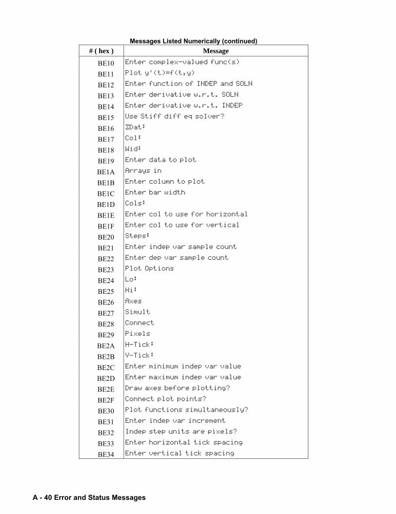
A - 40 Error and Status Messages
Messages Listed Numerically (continued) # ( hex ) Message
BE10 Enter complex-valued func(s)
BE11 Plot y'(t)=f(t,y)
BE12 Enter function of INDEP and SOLN
BE13 Enter derivative w.r.t. SOLN
BE14 Enter derivative w.r.t. INDEP
BE15 Use Stiff diff eq solver?
BE16 …Dat:
BE17 Col:
BE18 Wid:
BE19 Enter data to plot
BE1A Arrays in
BE1B Enter column to plot
BE1C Enter bar width
BE1D Cols:
BE1E Enter col to use for horizontal
BE1F Enter col to use for vertical
BE20 Steps:
BE21 Enter indep var sample count
BE22 Enter dep var sample count
BE23 Plot Options
BE24 Lo:
BE25 Hi:
BE26 Axes
BE27 Simult
BE28 Connect
BE29 Pixels
BE2A H-Tick:
BE2B V-Tick:
BE2C Enter minimum indep var value
BE2D Enter maximum indep var value
BE2E Draw axes before plotting?
BE2F Connect plot points?
BE30 Plot functions simultaneously?
BE31 Enter indep var increment
BE32 Indep step units are pixels?
BE33 Enter horizontal tick spacing
BE34 Enter vertical tick spacing
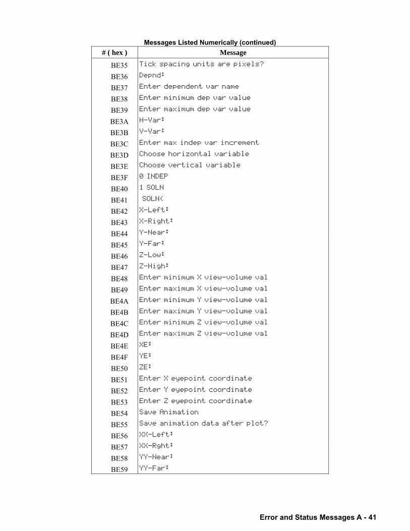
Error and Status Messages A - 41
Messages Listed Numerically (continued) # ( hex ) Message
BE35 Tick spacing units are pixels?
BE36 Depnd:
BE37 Enter dependent var name
BE38 Enter minimum dep var value
BE39 Enter maximum dep var value
BE3A H-Var:
BE3B V-Var:
BE3C Enter max indep var increment
BE3D Choose horizontal variable
BE3E Choose vertical variable
BE3F 0 INDEP
BE40 1 SOLN
BE41 SOLN(
BE42 X-Left:
BE43 X-Right:
BE44 Y-Near:
BE45 Y-Far:
BE46 Z-Low:
BE47 Z-High:
BE48 Enter minimum X view-volume val
BE49 Enter maximum X view-volume val
BE4A Enter minimum Y view-volume val
BE4B Enter maximum Y view-volume val
BE4C Enter minimum Z view-volume val
BE4D Enter maximum Z view-volume val
BE4E XE:
BE4F YE:
BE50 ZE:
BE51 Enter X eyepoint coordinate
BE52 Enter Y eyepoint coordinate
BE53 Enter Z eyepoint coordinate
BE54 Save Animation
BE55 Save animation data after plot?
BE56 XX-Left:
BE57 XX-Rght:
BE58 YY-Near:
BE59 YY-Far:
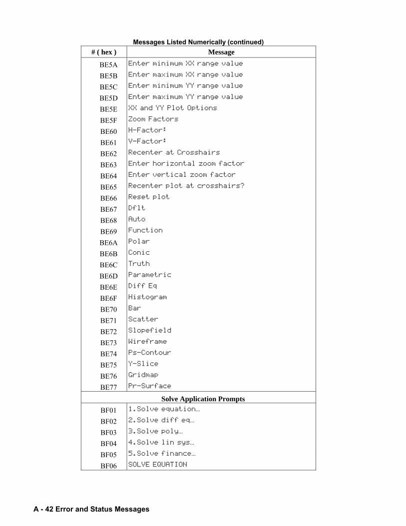
A - 42 Error and Status Messages
Messages Listed Numerically (continued) # ( hex ) Message
BE5A Enter minimum XX range value
BE5B Enter maximum XX range value
BE5C Enter minimum YY range value
BE5D Enter maximum YY range value
BE5E XX and YY Plot Options
BE5F Zoom Factors
BE60 H-Factor:
BE61 V-Factor:
BE62 Recenter at Crosshairs
BE63 Enter horizontal zoom factor
BE64 Enter vertical zoom factor
BE65 Recenter plot at crosshairs?
BE66 Reset plot
BE67 Dflt
BE68 Auto
BE69 Function
BE6A Polar
BE6B Conic
BE6C Truth
BE6D Parametric
BE6E Diff Eq
BE6F Histogram
BE70 Bar
BE71 Scatter
BE72 Slopefield
BE73 Wireframe
BE74 Ps-Contour
BE75 Y-Slice
BE76 Gridmap
BE77 Pr-Surface
Solve Application Prompts BF01 1.Solve equationÏ.
BF02 2.Solve diff eqÏ.
BF03 3.Solve polyÏ.
BF04 4.Solve lin sysÏ.
BF05 5.Solve financeÏ.
BF06 SOLVE EQUATION
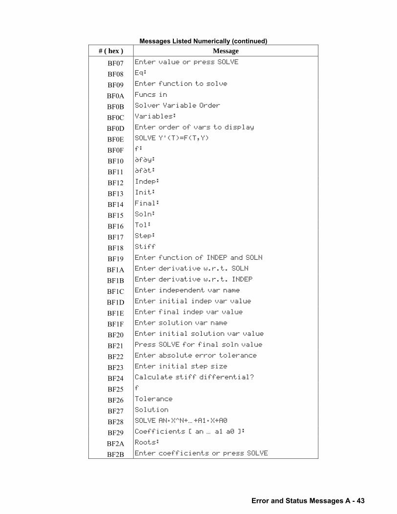
Error and Status Messages A - 43
Messages Listed Numerically (continued) # ( hex ) Message
BF07 Enter value or press SOLVE
BF08 Eq:
BF09 Enter function to solve
BF0A Funcs in
BF0B Solver Variable Order
BF0C Variables:
BF0D Enter order of vars to display
BF0E SOLVE Y'(T)=F(T,Y)
BF0F f:
BF10 ˆfˆy:
BF11 ˆfˆt:
BF12 Indep:
BF13 Init:
BF14 Final:
BF15 Soln:
BF16 Tol:
BF17 Step:
BF18 Stiff
BF19 Enter function of INDEP and SOLN
BF1A Enter derivative w.r.t. SOLN
BF1B Enter derivative w.r.t. INDEP
BF1C Enter independent var name
BF1D Enter initial indep var value
BF1E Enter final indep var value
BF1F Enter solution var name
BF20 Enter initial solution var value
BF21 Press SOLVE for final soln value
BF22 Enter absolute error tolerance
BF23 Enter initial step size
BF24 Calculate stiff differential?
BF25 f
BF26 Tolerance
BF27 Solution
BF28 SOLVE AN·X^N+Ï.+A1·X+A0
BF29 Coefficients [ an Ï. a1 a0 ]:
BF2A Roots:
BF2B Enter coefficients or press SOLVE
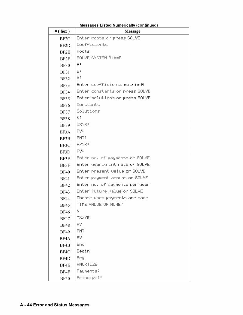
A - 44 Error and Status Messages
Messages Listed Numerically (continued) # ( hex ) Message
BF2C Enter roots or press SOLVE
BF2D Coefficients
BF2E Roots
BF2F SOLVE SYSTEM A·X=B
BF30 A:
BF31 B:
BF32 X:
BF33 Enter coefficients matrix A
BF34 Enter constants or press SOLVE
BF35 Enter solutions or press SOLVE
BF36 Constants
BF37 Solutions
BF38 N:
BF39 I%YR:
BF3A PV:
BF3B PMT:
BF3C P/YR:
BF3D FV:
BF3E Enter no. of payments or SOLVE
BF3F Enter yearly int rate or SOLVE
BF40 Enter present value or SOLVE
BF41 Enter payment amount or SOLVE
BF42 Enter no. of payments per year
BF43 Enter future value or SOLVE
BF44 Choose when payments are made
BF45 TIME VALUE OF MONEY
BF46 N
BF47 I%/YR
BF48 PV
BF49 PMT
BF4A FV
BF4B End
BF4C Begin
BF4D Beg
BF4E AMORTIZE
BF4F Payments:
BF50 Principal:

Error and Status Messages A - 45
Messages Listed Numerically (continued) # ( hex ) Message
BF51 Interest:
BF52 Balance:
BF53 Enter no. of payments to amort
BF54 Principal
BF55 Interest
BF56 Balance
C001 Unable to find root
CAS Messages DE01 denominator(s)
DE02 root(s)
DE03 last
DE04 obvious
DE05 factorizing
DE06 value
DE07 test(s)
DE08 searching
DE09 TAYLR of at
DE0A nth
DE0B is
DE0C numerator(s)
DE0D Less than
DE0E multiplicity
DE0F list of
DE10 at
DE11 factor(s)
DE12 Eigenvalues
DE13 Computing for
DE14 Root mult <
DE15 Numerical to symbolic
DE16 Invalid operator
DE17 Result:
DE18 Pivots
DE19 Press CONT to go on
DE1A Test
DE1B To be implemented
DE1C Unable to factor
DE1D Z is not = 1 mod 4
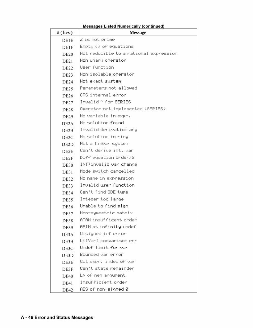
A - 46 Error and Status Messages
Messages Listed Numerically (continued) # ( hex ) Message
DE1E Z is not prime
DE1F Empty of equations
DE20 Not reducible to a rational expression
DE21 Non unary operator
DE22 User function
DE23 Non isolable operator
DE24 Not exact system
DE25 Parameters not allowed
DE26 CAS internal error
DE27 Invalid ^ for SERIES
DE28 Operator not implemented (SERIES)
DE29 No variable in expr.
DE2A No solution found
DE2B Invalid derivation arg
DE2C No solution in ring
DE2D Not a linear system
DE2E Can't derive int. var
DE2F Diff equation order>2
DE30 INT:invalid var change
DE31 Mode switch cancelled
DE32 No name in expression
DE33 Invalid user function
DE34 Can't find ODE type
DE35 Integer too large
DE36 Unable to find sign
DE37 Non-symmetric matrix
DE38 ATAN insufficent order
DE39 ASIN at infinity undef
DE3A Unsigned inf error
DE3B LN[Var] comparison err
DE3C Undef limit for var
DE3D Bounded var error
DE3E Got expr. indep of var
DE3F Can't state remainder
DE40 LN of neg argument
DE41 Insufficient order
DE42 ABS of non-signed 0
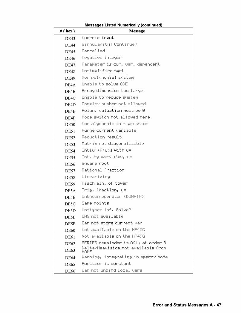
Error and Status Messages A - 47
Messages Listed Numerically (continued) # ( hex ) Message
DE43 Numeric input
DE44 Singularity! Continue?
DE45 Cancelled
DE46 Negative integer
DE47 Parameter is cur. var. dependent
DE48 Unsimplified sqrt
DE49 Non polynomial system
DE4A Unable to solve ODE
DE4B Array dimension too large
DE4C Unable to reduce system
DE4D Complex number not allowed
DE4E Polyn. valuation must be 0
DE4F Mode switch not allowed here
DE50 Non algebraic in expression
DE51 Purge current variable
DE52 Reduction result
DE53 Matrix not diagonalizable
DE54 Int[u'*F(u)] with u=
DE55 Int. by part u'*v, u=
DE56 Square root
DE57 Rational fraction
DE58 Linearizing
DE59 Risch alg. of tower
DE5A Trig. fraction, u=
DE5B Unknown operator (DOMAIN)
DE5C Same points
DE5D Unsigned inf. Solve?
DE5E CAS not available
DE5F Can not store current var
DE60 Not available on the HP40G
DE61 Not available on the HP49G
DE62 SERIES remainder is O(1) at order 3
DE63 Delta/Heaviside not available from HOME
DE64 Warning, integrating in approx mode
DE65 Function is constant
DE66 Can not unbind local vars
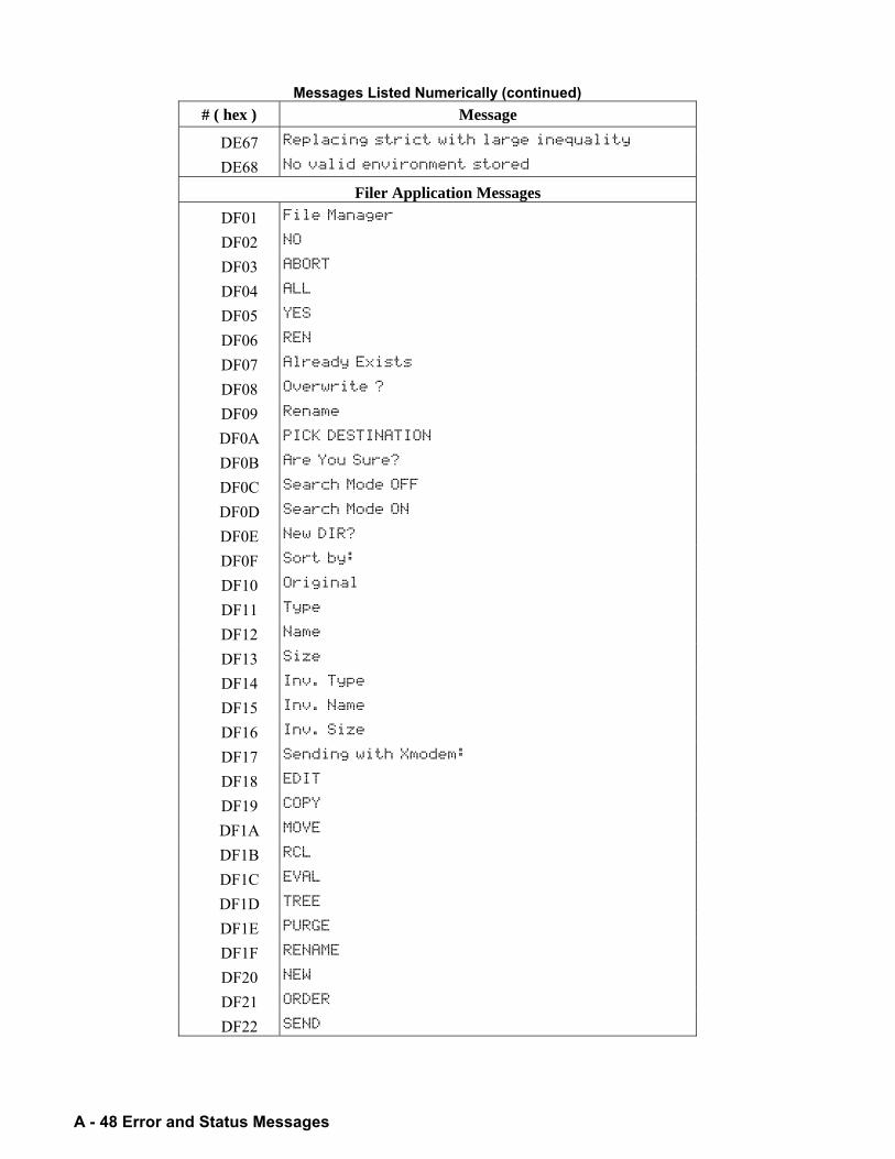
A - 48 Error and Status Messages
Messages Listed Numerically (continued) # ( hex ) Message
DE67 Replacing strict with large inequality
DE68 No valid environment stored
Filer Application Messages DF01 File Manager
DF02 NO
DF03 ABORT
DF04 ALL
DF05 YES
DF06 REN
DF07 Already Exists
DF08 Overwrite ?
DF09 Rename
DF0A PICK DESTINATION
DF0B Are You Sure?
DF0C Search Mode OFF
DF0D Search Mode ON
DF0E New DIR?
DF0F Sort by:
DF10 Original
DF11 Type
DF12 Name
DF13 Size
DF14 Inv. Type
DF15 Inv. Name
DF16 Inv. Size
DF17 Sending with Xmodem:
DF18 EDIT
DF19 COPY
DF1A MOVE
DF1B RCL
DF1C EVAL
DF1D TREE
DF1E PURGE
DF1F RENAME
DF20 NEW
DF21 ORDER
DF22 SEND
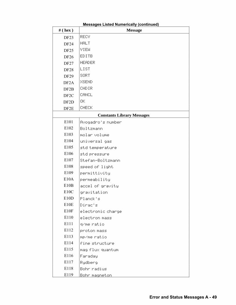
Error and Status Messages A - 49
Messages Listed Numerically (continued) # ( hex ) Message
DF23 RECV
DF24 HALT
DF25 VIEW
DF26 EDITB
DF27 HEADER
DF28 LIST
DF29 SORT
DF2A XSEND
DF2B CHDIR
DF2C CANCL
DF2D OK
DF2E CHECK
Constants Library Messages E101 Avogadro's number
E102 Boltzmann
E103 molar volume
E104 universal gas
E105 std temperature
E106 std pressure
E107 Stefan-Boltzmann
E108 speed of light
E109 permittivity
E10A permeability
E10B accel of gravity
E10C gravitation
E10D Planck's
E10E Dirac's
E10F electronic charge
E110 electron mass
E111 q/me ratio
E112 proton mass
E113 mp/me ratio
E114 fine structure
E115 mag flux quantum
E116 Faraday
E117 Rydberg
E118 Bohr radius
E119 Bohr magneton
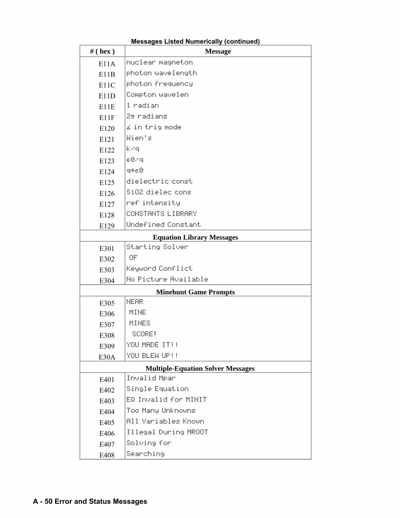
A - 50 Error and Status Messages
Messages Listed Numerically (continued) # ( hex ) Message
E11A nuclear magneton
E11B photon wavelength
E11C photon frequency
E11D Compton wavelen
E11E 1 radian
E11F 2‡ radians
E120 in trig mode
E121 Wien's
E122 k/q
E123 “0/q
E124 q*“0
E125 dielectric const
E126 SiO2 dielec cons
E127 ref intensity
E128 CONSTANTS LIBRARY
E129 Undefined Constant
Equation Library Messages E301 Starting Solver
E302 OF
E303 Keyword Conflict
E304 No Picture Available
Minehunt Game Prompts E305 NEAR
E306 MINE
E307 MINES
E308 SCORE:
E309 YOU MADE IT!!
E30A YOU BLEW UP!!
Multiple-Equation Solver Messages E401 Invalid Mpar
E402 Single Equation
E403 EQ Invalid for MINIT
E404 Too Many Unknowns
E405 All Variables Known
E406 Illegal During MROOT
E407 Solving for
E408 Searching
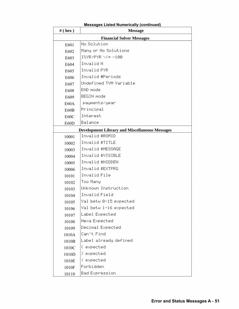
Error and Status Messages A - 51
Messages Listed Numerically (continued) # ( hex ) Message
Financial Solver Messages E601 No Solution
E602 Many or No Solutions
E603 I%YR/PYR \<= -100
E604 Invalid N
E605 Invalid PYR
E606 Invalid #Periods
E607 Undefined TVM Variable
E608 END mode
E609 BEGIN mode
E60A payments/year
E60B Principal
E60C Interest
E60D Balance
Development Library and Miscellaneous Messages 10001 Invalid $ROMID
10002 Invalid $TITLE
10003 Invalid $MESSAGE
10004 Invalid $VISIBLE
10005 Invalid $HIDDEN
10006 Invalid $EXTPRG
10101 Invalid File
10102 Too Many
10103 Unknown Instruction
10104 Invalid Field
10105 Val betw 0-15 expected
10106 Val betw 1-16 expected
10107 Label Expected
10108 Hexa Expected
10109 Decimal Expected
1010A Can't Find
1010B Label already defined
1010C expected
1010D expected
1010E ( expected
1010F Forbidden
10110 Bad Expression
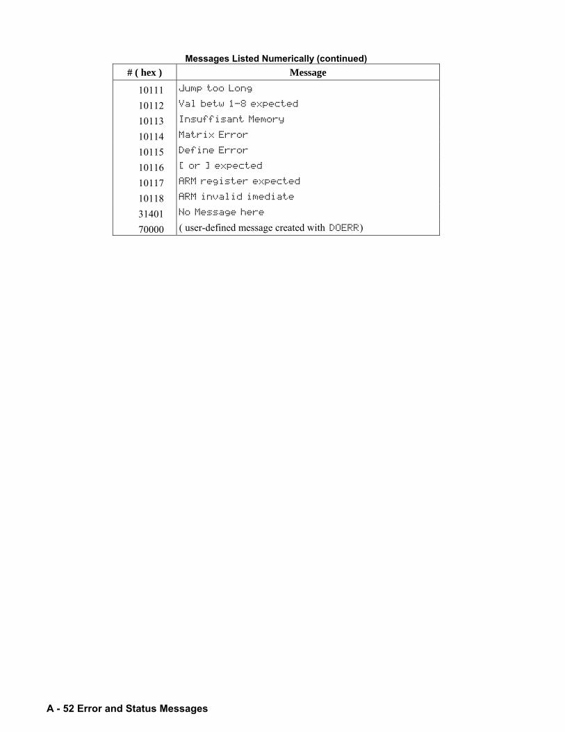
A - 52 Error and Status Messages
Messages Listed Numerically (continued) # ( hex ) Message
10111 Jump too Long
10112 Val betw 1-8 expected
10113 Insuffisant Memory
10114 Matrix Error
10115 Define Error
10116 [ or ] expected
10117 ARM register expected
10118 ARM invalid imediate
31401 No Message here
70000 ( user-defined message created with DOERR)
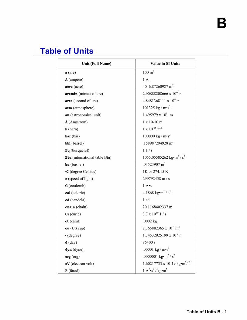
B
Table of Units B - 1
8.Table of Units Unit (Full Name) Value in SI Units
a (are) 100 m2
A (ampere) 1 A
acre (acre) 4046.87260987 m2
arcmin (minute of arc) 2.90888208666 x 10⁻⁴ r
arcs (second of arc) 4.8481368111 x 10⁻⁶ r
atm (atmosphere) 101325 kg / ms2
au (astronomical unit) 1.495979 x 10¹¹ m
Å (Angstrom) 1 x 10⁻¹⁰ m
b (barn) 1 x 10-28 m2
bar (bar) 100000 kg / ms2
bbl (barrel) .158987294928 m3
Bq (becquerel) 1 1 / s
Btu (international table Btu) 1055.05585262 kgm2 / s2
bu (bushel) .03523907 m3 oC (degree Celsius) 1K or 274.15 K
c (speed of light) 299792458 m / s
C (coulomb) 1 As
cal (calorie) 4.1868 kgm2 / s2
cd (candela) 1 cd
chain (chain) 20.1168402337 m
Ci (curie) 3.7 x 10¹⁰ 1 / s
ct (carat) .0002 kg
cu (US cup) 2.365882365 x 10⁻⁴ m3 o (degree) 1.74532925199 x 10⁻² r
d (day) 86400 s
dyn (dyne) .00001 kg / ms2
erg (erg) .0000001 kgm2 / s2
eV (electron volt) 1.60217733 x 10⁻¹⁹ kgm2/s2
F (farad) 1 A2s4 / kgm2
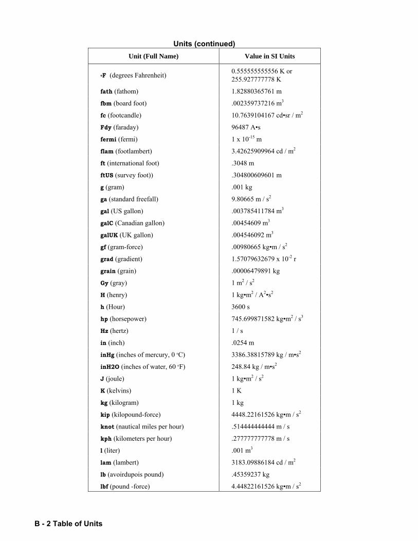
B - 2 Table of Units
Units (continued) Unit (Full Name) Value in SI Units
oF (degrees Fahrenheit) 0.555555555556 K or 255.927777778 K
fath (fathom) 1.82880365761 m
fbm (board foot) .002359737216 m3
fc (footcandle) 10.7639104167 cdsr / m2
Fdy (faraday) 96487 As
fermi (fermi) 1 x 10-15 m
flam (footlambert) 3.42625909964 cd / m2
ft (international foot) .3048 m
ftUS (survey foot)) .304800609601 m
g (gram) .001 kg
ga (standard freefall) 9.80665 m / s2
gal (US gallon) .003785411784 m3
galC (Canadian gallon) .00454609 m3
galUK (UK gallon) .004546092 m3
gf (gram-force) .00980665 kgm / s2
grad (gradient) 1.57079632679 x 10⁻² r
grain (grain) .00006479891 kg
Gy (gray) 1 m2 / s2
H (henry) 1 kgm2 / A2s2
h (Hour) 3600 s
hp (horsepower) 745.699871582 kgm2 / s3
Hz (hertz) 1 / s
in (inch) .0254 m
inHg (inches of mercury, 0 oC) 3386.38815789 kg / ms2
inH2O (inches of water, 60 oF) 248.84 kg / ms2
J (joule) 1 kgm2 / s2
K (kelvins) 1 K
kg (kilogram) 1 kg
kip (kilopound-force) 4448.22161526 kgm / s2
knot (nautical miles per hour) .514444444444 m / s
kph (kilometers per hour) .277777777778 m / s
l (liter) .001 m3
lam (lambert) 3183.09886184 cd / m2
lb (avoirdupois pound) .45359237 kg
lbf (pound -force) 4.44822161526 kgm / s2
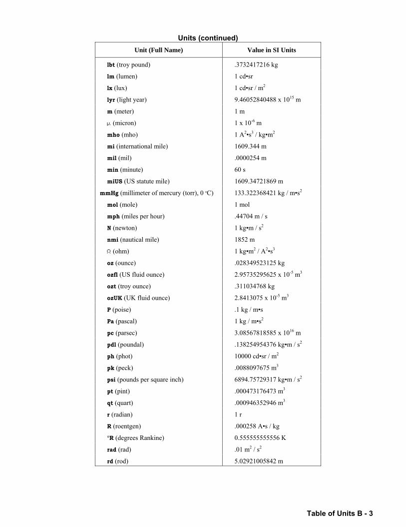
Table of Units B - 3
Units (continued) Unit (Full Name) Value in SI Units
lbt (troy pound) .3732417216 kg
lm (lumen) 1 cdsr
lx (lux) 1 cdsr / m2
lyr (light year) 9.46052840488 x 10¹⁵ m
m (meter) 1 m
µ (micron) 1 x 10⁻⁶ m
mho (mho) 1 A2s3 / kgm2
mi (international mile) 1609.344 m
mil (mil) .0000254 m
min (minute) 60 s
miUS (US statute mile) 1609.34721869 m
mmHg (millimeter of mercury (torr), 0 oC) 133.322368421 kg / ms2
mol (mole) 1 mol
mph (miles per hour) .44704 m / s
N (newton) 1 kgm / s2
nmi (nautical mile) 1852 m
(ohm) 1 kgm2 / A2s3
oz (ounce) .028349523125 kg
ozfl (US fluid ounce) 2.95735295625 x 10⁻⁵ m3
ozt (troy ounce) .311034768 kg
ozUK (UK fluid ounce) 2.8413075 x 10⁻⁵ m3
P (poise) .1 kg / ms
Pa (pascal) 1 kg / ms2
pc (parsec) 3.08567818585 x 10¹⁶ m
pdl (poundal) .138254954376 kgm / s2
ph (phot) 10000 cdsr / m2
pk (peck) .0088097675 m3
psi (pounds per square inch) 6894.75729317 kgm / s2
pt (pint) .000473176473 m3
qt (quart) .000946352946 m3
r (radian) 1 r
R (roentgen) .000258 As / kg
°R (degrees Rankine) 0.555555555556 K
rad (rad) .01 m2 / s2
rd (rod) 5.02921005842 m
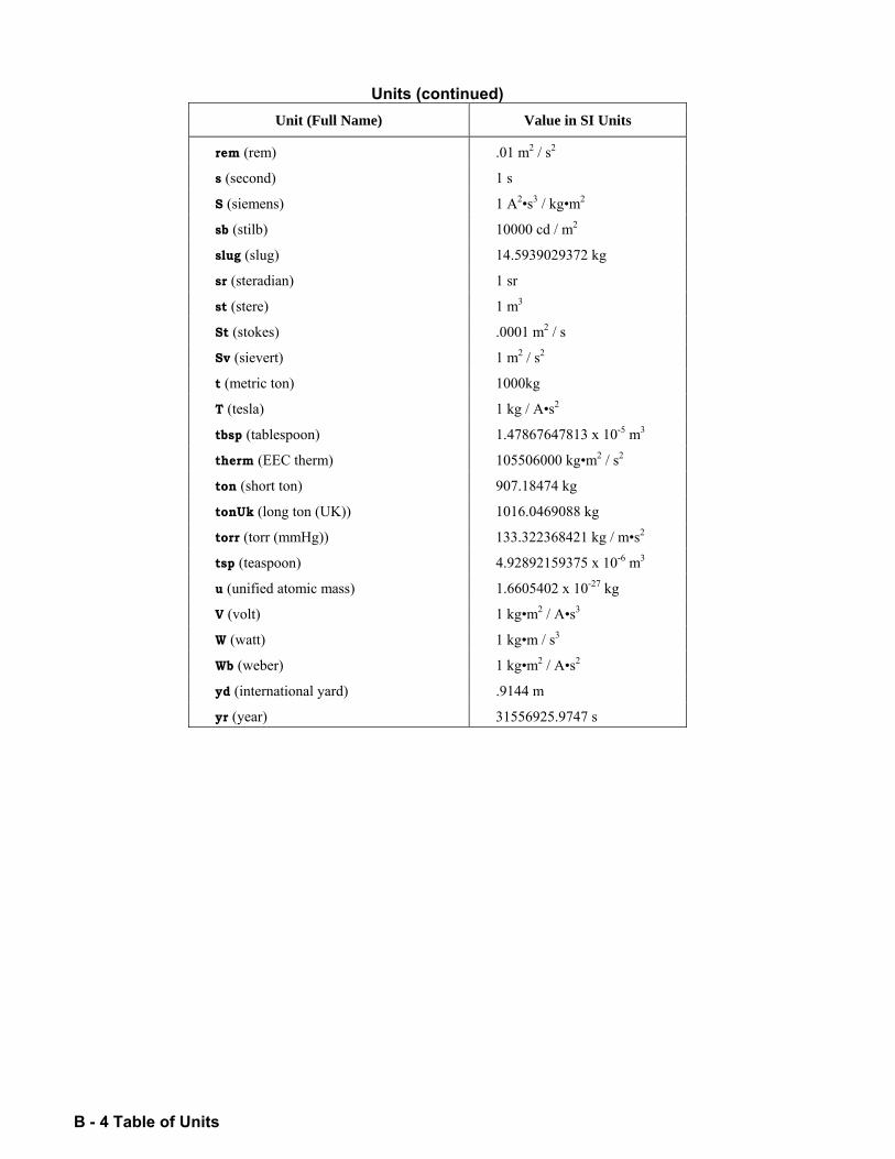
B - 4 Table of Units
Units (continued) Unit (Full Name) Value in SI Units
rem (rem) .01 m2 / s2
s (second) 1 s
S (siemens) 1 A2s3 / kgm2
sb (stilb) 10000 cd / m2
slug (slug) 14.5939029372 kg
sr (steradian) 1 sr
st (stere) 1 m3
St (stokes) .0001 m2 / s
Sv (sievert) 1 m2 / s2
t (metric ton) 1000kg
T (tesla) 1 kg / As2
tbsp (tablespoon) 1.47867647813 x 10⁻⁵ m3
therm (EEC therm) 105506000 kgm2 / s2
ton (short ton) 907.18474 kg
tonUk (long ton (UK)) 1016.0469088 kg
torr (torr (mmHg)) 133.322368421 kg / ms2
tsp (teaspoon) 4.92892159375 x 10⁻⁶ m3
u (unified atomic mass) 1.6605402 x 10⁻²⁷ kg
V (volt) 1 kgm2 / As3
W (watt) 1 kgm / s3
Wb (weber) 1 kgm2 / As2
yd (international yard) .9144 m
yr (year) 31556925.9747 s
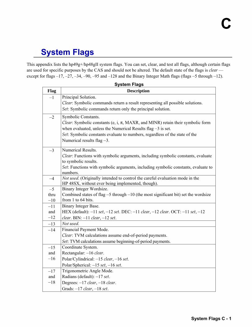
C
System Flags C - 1
9.System Flags This appendix lists the hp49g+/hp48gII system flags. You can set, clear, and test all flags, although certain flags are used for specific purposes by the CAS and should not be altered. The default state of the flags is clear except for flags 17, 27, 34, 90, 95 and 128 and the Binary Integer Math flags (flags 5 through 12).
System Flags Flag Description 1 Principal Solution.
Clear: Symbolic commands return a result representing all possible solutions. Set: Symbolic commands return only the principal solution.
2 Symbolic Constants. Clear: Symbolic constants (e, i, π, MAXR, and MINR) retain their symbolic form when evaluated, unless the Numerical Results flag 3 is set. Set: Symbolic constants evaluate to numbers, regardless of the state of the Numerical results flag 3.
3 Numerical Results. Clear: Functions with symbolic arguments, including symbolic constants, evaluate to symbolic results. Set: Functions with symbolic arguments, including symbolic constants, evaluate to numbers.
4 Not used. (Originally intended to control the careful evaluation mode in the HP 48SX, without ever being implemented, though).
5 thru 10
Binary Integer Wordsize. Combined states of flag 5 through 10 (the most significant bit) set the wordsize from 1 to 64 bits.
11 and 12
Binary Integer Base. HEX (default): 11 set, 12 set. DEC: 11 clear, 12 clear. OCT: 11 set, 12 clear. BIN: 11 clear, 12 set.
13 Not used. 14 Financial Payment Mode.
Clear: TVM calculations assume end-of-period payments. Set: TVM calculations assume beginning-of-period payments.
15 and 16
Coordinate System. Rectangular: 16 clear. Polar/Cylindrical: 15 clear, 16 set. Polar/Spherical: 15 set, 16 set.
17 and 18
Trigonometric Angle Mode. Radians (default): 17 set. Degrees: 17 clear, 18 clear. Grads: 17 clear, 18 set.
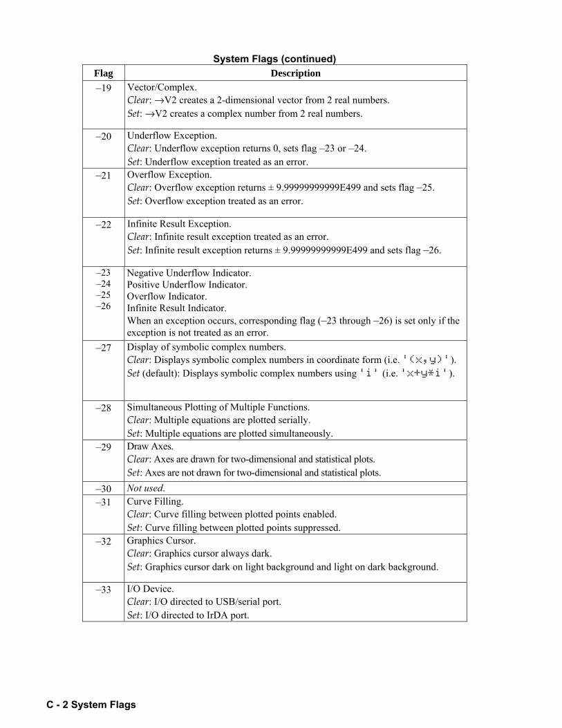
C - 2 System Flags
System Flags (continued) Flag Description 19 Vector/Complex.
Clear: →V2 creates a 2-dimensional vector from 2 real numbers. Set: →V2 creates a complex number from 2 real numbers.
20 Underflow Exception. Clear: Underflow exception returns 0, sets flag 23 or 24. Set: Underflow exception treated as an error.
21 Overflow Exception. Clear: Overflow exception returns ± 9.99999999999E499 and sets flag 25. Set: Overflow exception treated as an error.
22 Infinite Result Exception. Clear: Infinite result exception treated as an error. Set: Infinite result exception returns ± 9.99999999999E499 and sets flag 26.
23 24 25 26
Negative Underflow Indicator. Positive Underflow Indicator. Overflow Indicator. Infinite Result Indicator. When an exception occurs, corresponding flag (23 through 26) is set only if the exception is not treated as an error.
27 Display of symbolic complex numbers. Clear: Displays symbolic complex numbers in coordinate form (i.e. '(x,y)'). Set (default): Displays symbolic complex numbers using 'i' (i.e. 'x+y*i').
28 Simultaneous Plotting of Multiple Functions. Clear: Multiple equations are plotted serially. Set: Multiple equations are plotted simultaneously.
29 Draw Axes. Clear: Axes are drawn for two-dimensional and statistical plots. Set: Axes are not drawn for two-dimensional and statistical plots.
30 Not used. 31 Curve Filling.
Clear: Curve filling between plotted points enabled. Set: Curve filling between plotted points suppressed.
32 Graphics Cursor. Clear: Graphics cursor always dark. Set: Graphics cursor dark on light background and light on dark background.
33 I/O Device. Clear: I/O directed to USB/serial port. Set: I/O directed to IrDA port.
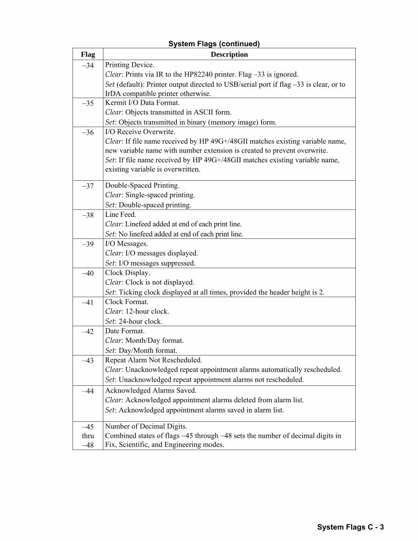
System Flags C - 3
System Flags (continued) Flag Description 34 Printing Device.
Clear: Prints via IR to the HP82240 printer. Flag 33 is ignored. Set (default): Printer output directed to USB/serial port if flag 33 is clear, or to IrDA compatible printer otherwise.
35 Kermit I/O Data Format. Clear: Objects transmitted in ASCII form. Set: Objects transmitted in binary (memory image) form.
36 I/O Receive Overwrite. Clear: If file name received by HP 49G+/48GII matches existing variable name, new variable name with number extension is created to prevent overwrite. Set: If file name received by HP 49G+/48GII matches existing variable name, existing variable is overwritten.
37 Double-Spaced Printing. Clear: Single-spaced printing. Set: Double-spaced printing.
38 Line Feed. Clear: Linefeed added at end of each print line. Set: No linefeed added at end of each print line.
39 I/O Messages. Clear: I/O messages displayed. Set: I/O messages suppressed.
40 Clock Display. Clear: Clock is not displayed. Set: Ticking clock displayed at all times, provided the header height is 2.
41 Clock Format. Clear: 12-hour clock. Set: 24-hour clock.
42 Date Format. Clear: Month/Day format. Set: Day/Month format.
43 Repeat Alarm Not Rescheduled. Clear: Unacknowledged repeat appointment alarms automatically rescheduled. Set: Unacknowledged repeat appointment alarms not rescheduled.
44 Acknowledged Alarms Saved. Clear: Acknowledged appointment alarms deleted from alarm list. Set: Acknowledged appointment alarms saved in alarm list.
45 thru 48
Number of Decimal Digits. Combined states of flags 45 through 48 sets the number of decimal digits in Fix, Scientific, and Engineering modes.
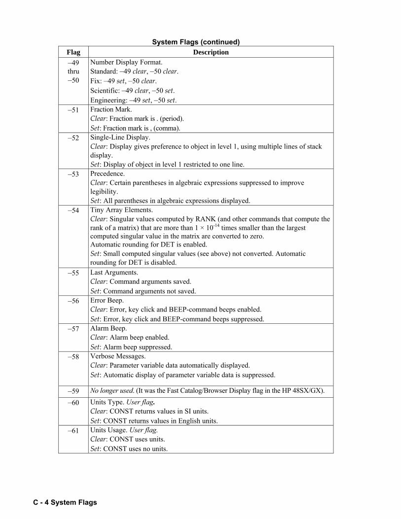
C - 4 System Flags
System Flags (continued) Flag Description 49 thru 50
Number Display Format. Standard: 49 clear, 50 clear. Fix: 49 set, 50 clear. Scientific: 49 clear, 50 set. Engineering: 49 set, 50 set.
51 Fraction Mark. Clear: Fraction mark is . (period). Set: Fraction mark is , (comma).
52 Single-Line Display. Clear: Display gives preference to object in level 1, using multiple lines of stack display. Set: Display of object in level 1 restricted to one line.
53 Precedence. Clear: Certain parentheses in algebraic expressions suppressed to improve legibility. Set: All parentheses in algebraic expressions displayed.
54 Tiny Array Elements. Clear: Singular values computed by RANK (and other commands that compute the rank of a matrix) that are more than 1 × 10-14 times smaller than the largest computed singular value in the matrix are converted to zero. Automatic rounding for DET is enabled. Set: Small computed singular values (see above) not converted. Automatic rounding for DET is disabled.
55 Last Arguments. Clear: Command arguments saved. Set: Command arguments not saved.
56 Error Beep. Clear: Error, key click and BEEP-command beeps enabled. Set: Error, key click and BEEP-command beeps suppressed.
57 Alarm Beep. Clear: Alarm beep enabled. Set: Alarm beep suppressed.
58 Verbose Messages. Clear: Parameter variable data automatically displayed. Set: Automatic display of parameter variable data is suppressed.
59 No longer used. (It was the Fast Catalog/Browser Display flag in the HP 48SX/GX).
60 Units Type. User flag. Clear: CONST returns values in SI units. Set: CONST returns values in English units.
61 Units Usage. User flag. Clear: CONST uses units. Set: CONST uses no units.
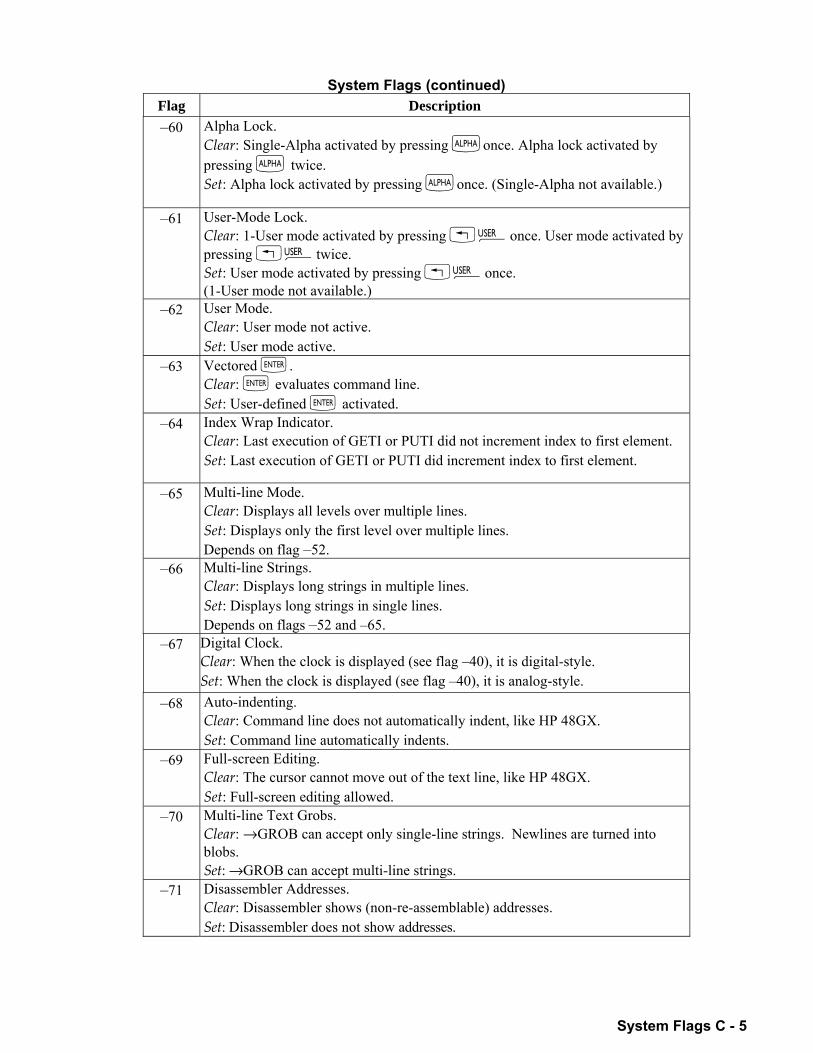
System Flags C - 5
System Flags (continued) Flag Description 60 Alpha Lock.
Clear: Single-Alpha activated by pressing ~once. Alpha lock activated by pressing ~ twice. Set: Alpha lock activated by pressing ~once. (Single-Alpha not available.)
61 User-Mode Lock. Clear: 1-User mode activated by pressing Ìonce. User mode activated by pressing Ìtwice. Set: User mode activated by pressing Ìonce. (1-User mode not available.)
62 User Mode. Clear: User mode not active. Set: User mode active.
63 Vectored `. Clear: ` evaluates command line. Set: User-defined ` activated.
64 Index Wrap Indicator. Clear: Last execution of GETI or PUTI did not increment index to first element. Set: Last execution of GETI or PUTI did increment index to first element.
65 Multi-line Mode. Clear: Displays all levels over multiple lines. Set: Displays only the first level over multiple lines. Depends on flag 52.
66 Multi-line Strings. Clear: Displays long strings in multiple lines. Set: Displays long strings in single lines. Depends on flags 52 and 65.
67 Digital Clock. Clear: When the clock is displayed (see flag 40), it is digital-style. Set: When the clock is displayed (see flag 40), it is analog-style.
68 Auto-indenting. Clear: Command line does not automatically indent, like HP 48GX. Set: Command line automatically indents.
69 Full-screen Editing. Clear: The cursor cannot move out of the text line, like HP 48GX. Set: Full-screen editing allowed.
70 Multi-line Text Grobs. Clear: →GROB can accept only single-line strings. Newlines are turned into blobs. Set: →GROB can accept multi-line strings.
71 Disassembler Addresses. Clear: Disassembler shows (non-re-assemblable) addresses. Set: Disassembler does not show addresses.
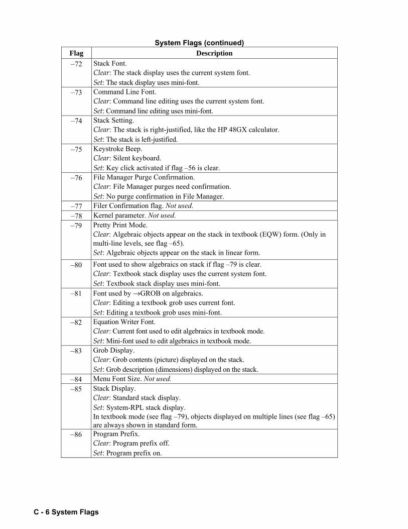
C - 6 System Flags
System Flags (continued) Flag Description 72 Stack Font.
Clear: The stack display uses the current system font. Set: The stack display uses mini-font.
73 Command Line Font. Clear: Command line editing uses the current system font. Set: Command line editing uses mini-font.
74 Stack Setting. Clear: The stack is right-justified, like the HP 48GX calculator. Set: The stack is left-justified.
75 Keystroke Beep. Clear: Silent keyboard. Set: Key click activated if flag 56 is clear.
76 File Manager Purge Confirmation. Clear: File Manager purges need confirmation. Set: No purge confirmation in File Manager.
77 Filer Confirmation flag. Not used. 78 Kernel parameter. Not used. 79
Pretty Print Mode. Clear: Algebraic objects appear on the stack in textbook (EQW) form. (Only in multi-line levels, see flag 65). Set: Algebraic objects appear on the stack in linear form.
80 Font used to show algebraics on stack if flag 79 is clear. Clear: Textbook stack display uses the current system font. Set: Textbook stack display uses mini-font.
81 Font used by →GROB on algebraics. Clear: Editing a textbook grob uses current font. Set: Editing a textbook grob uses mini-font.
82 Equation Writer Font. Clear: Current font used to edit algebraics in textbook mode. Set: Mini-font used to edit algebraics in textbook mode.
83 Grob Display. Clear: Grob contents (picture) displayed on the stack. Set: Grob description (dimensions) displayed on the stack.
84 Menu Font Size. Not used. 85 Stack Display.
Clear: Standard stack display. Set: System-RPL stack display. In textbook mode (see flag 79), objects displayed on multiple lines (see flag 65) are always shown in standard form.
86 Program Prefix. Clear: Program prefix off. Set: Program prefix on.
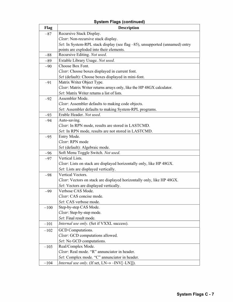
System Flags C - 7
System Flags (continued) Flag Description 87 Recursive Stack Display.
Clear: Non-recursive stack display. Set: In System-RPL stack display (see flag 85), unsupported (unnamed) entry points are exploded into their elements.
88 Recursive Editing. Not used. 89 Extable Library Usage. Not used. 90 Choose Box Font.
Clear: Choose boxes displayed in current font. Set (default): Choose boxes displayed in mini-font.
91 Matrix Writer Object Type. Clear: Matrix Writer returns arrays only, like the HP 48GX calculator. Set: Matrix Writer returns a list of lists.
92 Assembler Mode. Clear: Assembler defaults to making code objects. Set: Assembler defaults to making System-RPL programs.
93 Erable Header. Not used. 94 Auto-saving.
Clear: In RPN mode, results are stored in LASTCMD. Set: In RPN mode, results are not stored in LASTCMD.
95 Entry Mode. Clear: RPN mode Set (default): Algebraic mode.
96 Soft Menu Toggle Switch. Not used. 97 Vertical Lists.
Clear: Lists on stack are displayed horizontally only, like HP 48GX. Set: Lists are displayed vertically.
98 Vertical Vectors. Clear: Vectors on stack are displayed horizontally only, like HP 48GX. Set: Vectors are displayed vertically.
99 Verbose CAS Mode. Clear: CAS concise mode. Set: CAS verbose mode.
100 Step-by-step CAS Mode. Clear: Step-by-step mode. Set: Final result mode.
101 Internal use only. (Set if VXXL success).
102 GCD Computations. Clear: GCD computations allowed. Set: No GCD computations.
103 Real/Complex Mode. Clear: Real mode. R annunciator in header. Set: Complex mode. C annunciator in header.
104 Internal use only. (If set, LN→ INV[LN]]).
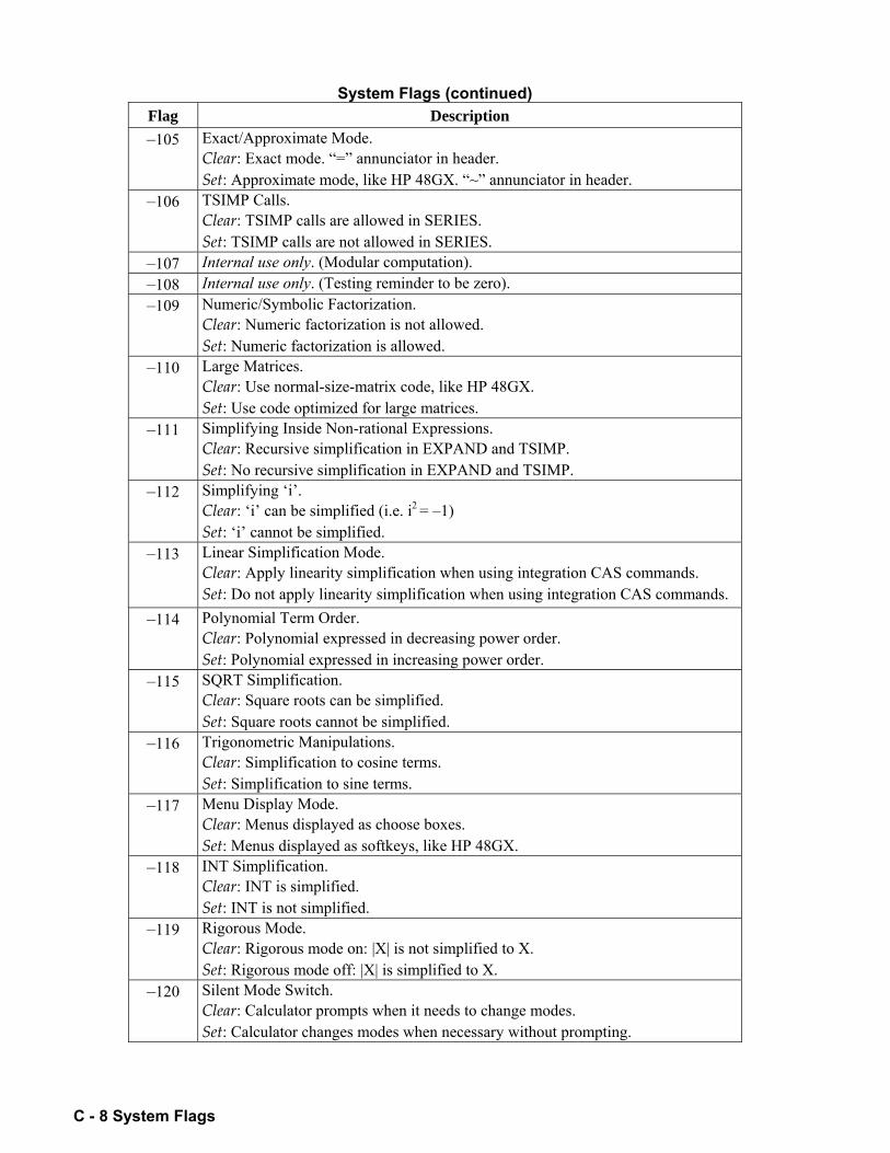
C - 8 System Flags
System Flags (continued) Flag Description 105 Exact/Approximate Mode.
Clear: Exact mode. = annunciator in header. Set: Approximate mode, like HP 48GX. ~ annunciator in header.
106 TSIMP Calls. Clear: TSIMP calls are allowed in SERIES. Set: TSIMP calls are not allowed in SERIES.
107 Internal use only. (Modular computation). 108 Internal use only. (Testing reminder to be zero). 109 Numeric/Symbolic Factorization.
Clear: Numeric factorization is not allowed. Set: Numeric factorization is allowed.
110 Large Matrices. Clear: Use normal-size-matrix code, like HP 48GX. Set: Use code optimized for large matrices.
111 Simplifying Inside Non-rational Expressions. Clear: Recursive simplification in EXPAND and TSIMP. Set: No recursive simplification in EXPAND and TSIMP.
112 Simplifying i. Clear: i can be simplified (i.e. i2 = 1) Set: i cannot be simplified.
113 Linear Simplification Mode. Clear: Apply linearity simplification when using integration CAS commands. Set: Do not apply linearity simplification when using integration CAS commands.
114 Polynomial Term Order. Clear: Polynomial expressed in decreasing power order. Set: Polynomial expressed in increasing power order.
115 SQRT Simplification. Clear: Square roots can be simplified. Set: Square roots cannot be simplified.
116 Trigonometric Manipulations. Clear: Simplification to cosine terms. Set: Simplification to sine terms.
117 Menu Display Mode. Clear: Menus displayed as choose boxes. Set: Menus displayed as softkeys, like HP 48GX.
118 INT Simplification. Clear: INT is simplified. Set: INT is not simplified.
119 Rigorous Mode. Clear: Rigorous mode on: |X| is not simplified to X. Set: Rigorous mode off: |X| is simplified to X.
120 Silent Mode Switch. Clear: Calculator prompts when it needs to change modes. Set: Calculator changes modes when necessary without prompting.
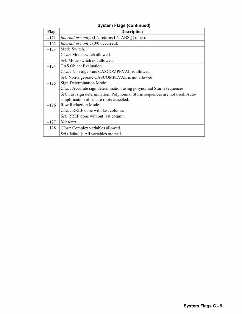
System Flags C - 9
System Flags (continued) Flag Description 121 Internal use only. (LN returns LN[ABS()] if set). 122 Internal use only. (0/0 occurred). 123 Mode Switch.
Clear: Mode switch allowed. Set: Mode switch not allowed.
124 CAS Object Evaluation. Clear: Non-algebraic CASCOMPEVAL is allowed. Set: Non-algebraic CASCOMPEVAL is not allowed.
125 Sign Determination Mode. Clear: Accurate sign determination using polynomial Sturm sequences. Set: Fast sign determination. Polynomial Sturm sequences are not used. Auto-simplification of square roots canceled.
126 Row Reduction Mode. Clear: RREF done with last column. Set: RREF done without last column.
127 Not used. 128 Clear: Complex variables allowed.
Set (default): All variables are real.

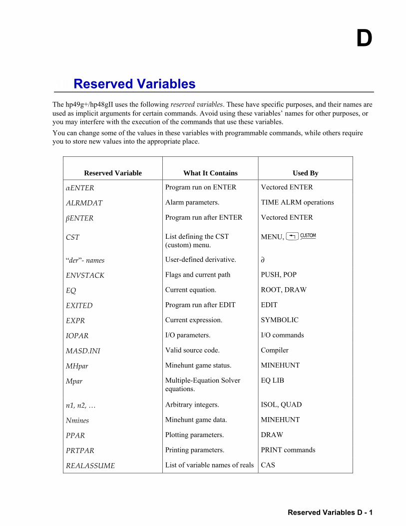
D
Reserved Variables D - 1
10.Reserved Variables The hp49g+/hp48gII uses the following reserved variables. These have specific purposes, and their names are used as implicit arguments for certain commands. Avoid using these variables names for other purposes, or you may interfere with the execution of the commands that use these variables. You can change some of the values in these variables with programmable commands, while others require you to store new values into the appropriate place.
Reserved Variable What It Contains Used By
αENTER Program run on ENTER Vectored ENTER
ALRMDAT Alarm parameters. TIME ALRM operations
βENTER Program run after ENTER Vectored ENTER
CST List defining the CST (custom) menu.
MENU, £
der- names User-defined derivative. ∂
ENVSTACK Flags and current path PUSH, POP
EQ Current equation. ROOT, DRAW
EXITED Program run after EDIT EDIT
EXPR Current expression. SYMBOLIC
IOPAR I/O parameters. I/O commands
MASD.INI Valid source code. Compiler
MHpar Minehunt game status. MINEHUNT
Mpar Multiple-Equation Solver equations.
EQ LIB
n1, n2, Arbitrary integers. ISOL, QUAD
Nmines Minehunt game data. MINEHUNT
PPAR Plotting parameters. DRAW
PRTPAR Printing parameters. PRINT commands
REALASSUME List of variable names of reals CAS
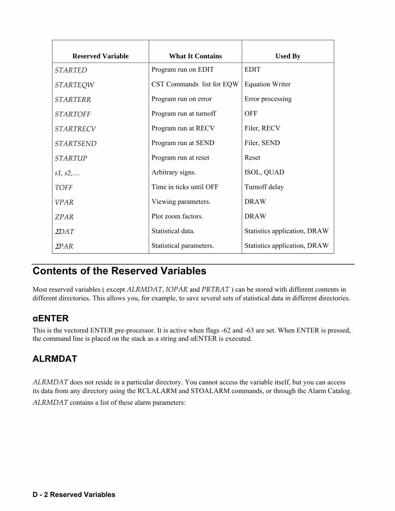
D - 2 Reserved Variables
Reserved Variable What It Contains Used By
STARTED Program run on EDIT EDIT
STARTEQW CST Commands list for EQW Equation Writer
STARTERR Program run on error Error processing
STARTOFF Program run at turnoff OFF
STARTRECV Program run at RECV Filer, RECV
STARTSEND Program run at SEND Filer, SEND
STARTUP Program run at reset Reset
s1, s2, Arbitrary signs. ISOL, QUAD
TOFF Time in ticks until OFF Turnoff delay
VPAR Viewing parameters. DRAW
ZPAR Plot zoom factors. DRAW
ΣDAT Statistical data. Statistics application, DRAW
ΣPAR Statistical parameters. Statistics application, DRAW
Contents of the Reserved Variables Most reserved variables ( except ALRMDAT, IOPAR and PRTRAT ) can be stored with different contents in different directories. This allows you, for example, to save several sets of statistical data in different directories. αENTER This is the vectored ENTER pre-processor. It is active when flags -62 and -63 are set. When ENTER is pressed, the command line is placed on the stack as a string and αENTER is executed. ALRMDAT ALRMDAT does not reside in a particular directory. You cannot access the variable itself, but you can access its data from any directory using the RCLALARM and STOALARM commands, or through the Alarm Catalog. ALRMDAT contains a list of these alarm parameters:
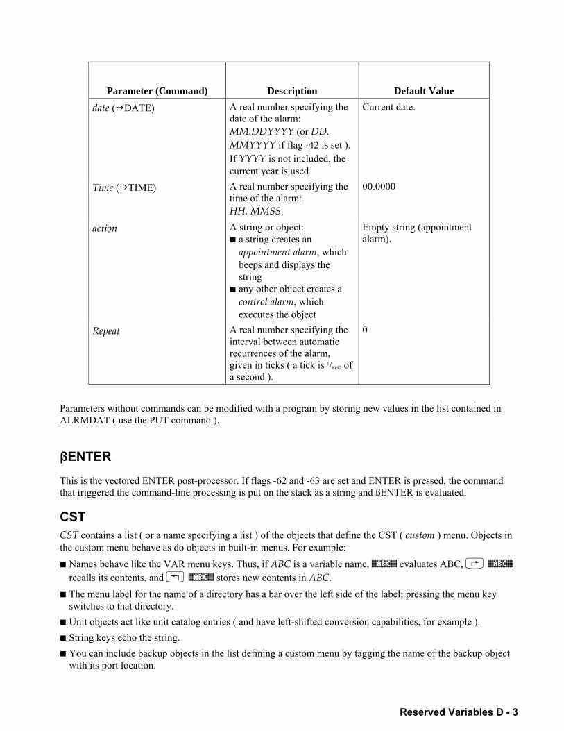
Reserved Variables D - 3
Parameter (Command) Description Default Value
date ("DATE) A real number specifying the date of the alarm: MM.DDYYYY (or DD. MMYYYY if flag -42 is set ). If YYYY is not included, the current year is used.
Current date.
Time ("TIME) A real number specifying the time of the alarm: HH. MMSS.
00.0000
action A string or object: ! a string creates an
appointment alarm, which beeps and displays the string
! any other object creates a control alarm, which executes the object
Empty string (appointment alarm).
Repeat A real number specifying the interval between automatic recurrences of the alarm, given in ticks ( a tick is 1/8192 of a second ).
0
Parameters without commands can be modified with a program by storing new values in the list contained in ALRMDAT ( use the PUT command ).
βENTER This is the vectored ENTER post-processor. If flags -62 and -63 are set and ENTER is pressed, the command that triggered the command-line processing is put on the stack as a string and ßENTER is evaluated. CST CST contains a list ( or a name specifying a list ) of the objects that define the CST ( custom ) menu. Objects in the custom menu behave as do objects in built-in menus. For example: ! Names behave like the VAR menu keys. Thus, if ABC is a variable name, %ABC% evaluates ABC, %ABC%
recalls its contents, and %ABC% stores new contents in ABC. ! The menu label for the name of a directory has a bar over the left side of the label; pressing the menu key
switches to that directory. ! Unit objects act like unit catalog entries ( and have left-shifted conversion capabilities, for example ). ! String keys echo the string. ! You can include backup objects in the list defining a custom menu by tagging the name of the backup object
with its port location.
D - 4 Reserved Variables
You can specify menu labels and key actions independently by replacing a single object within the custom-menu list with a list of the form label-object action-object .
To provide different shifted actions for custom menu keys, action-object can be a list containing three action objects in this order: ! The unshifted action ( required if you want to specify the shifted actions ). ! The left-shifted action. ! The right-shifted action. ENVSTACK ENVSTACK is a variable stored in the CAS directory. It is used by PUSH and POP to save the status of flags and the current directory. (PUSH saves the data in ENVSTACK; POP restores it.) EQ EQ contains the current equation or the name of the variable containing the current equation,
EQ supplies the equation for ROOT, as well as for the plotting command DRAW. (ΣDAT supplies the information when the plot type is HISTOGRAM, BAR, or SCATTER.) The object in EQ can be an algebraic object, a number, a name, or a program. How DRAW interprets EQ depends on the plot type. For graphics use, EQ can also be a list of equations or other objects. If EQ contains a list, then DRAW treats each object in turn as the current equation, and plots them successively. However, ROOT in the HP Solve application cannot solve an EQ containing al list.
To alter the contents of EQ, use the command STEQ. EXITED EXITED can be stored in any directory. If there is an EXITED program that exists in the path, it will be called upon exiting the command line. This can be used in conjunction with STARTED, for instance, to set a header size of 0 when entering the command line and restore it to 2 when exiting (in order to increase the editor window size). Note, this is only valid when entering the command line through a EDIT function. EXPR EXPR contains the current algebraic expression ( or the name of the variable containing the current expression ) used by the SYMBOLIC application and its associated commands. The object in EQ must be an algebraic or a name. IOPAR IOPAR is a variable in the HOME directory that contains a list of the I/O parameters needed for a communications link with a computer. It is created the first time you transfer data or open the serial port (OPENIO ), and is automatically updated whenever you change the I/O settings. All IOPAR parameters are integers.
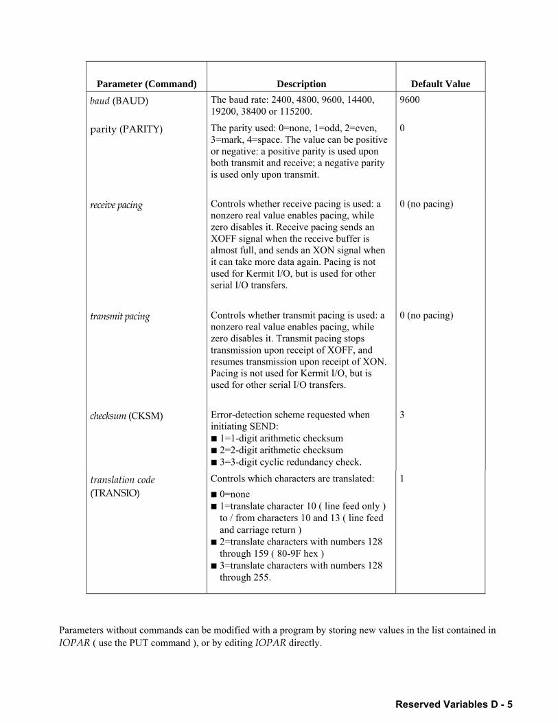
Reserved Variables D - 5
Parameter (Command) Description Default Value
baud (BAUD) The baud rate: 2400, 4800, 9600, 14400, 19200, 38400 or 115200.
9600
parity (PARITY) The parity used: 0=none, 1=odd, 2=even, 3=mark, 4=space. The value can be positive or negative: a positive parity is used upon both transmit and receive; a negative parity is used only upon transmit.
0
receive pacing Controls whether receive pacing is used: a nonzero real value enables pacing, while zero disables it. Receive pacing sends an XOFF signal when the receive buffer is almost full, and sends an XON signal when it can take more data again. Pacing is not used for Kermit I/O, but is used for other serial I/O transfers.
0 (no pacing)
transmit pacing Controls whether transmit pacing is used: a nonzero real value enables pacing, while zero disables it. Transmit pacing stops transmission upon receipt of XOFF, and resumes transmission upon receipt of XON. Pacing is not used for Kermit I/O, but is used for other serial I/O transfers.
0 (no pacing)
checksum (CKSM) Error-detection scheme requested when initiating SEND: ! 1=1-digit arithmetic checksum ! 2=2-digit arithmetic checksum ! 3=3-digit cyclic redundancy check.
3
translation code (TRANSIO)
Controls which characters are translated: ! 0=none ! 1=translate character 10 ( line feed only )
to / from characters 10 and 13 ( line feed and carriage return )
! 2=translate characters with numbers 128 through 159 ( 80-9F hex )
! 3=translate characters with numbers 128 through 255.
1
Parameters without commands can be modified with a program by storing new values in the list contained in IOPAR ( use the PUT command ), or by editing IOPAR directly.
D - 6 Reserved Variables
MASD.INI MASD.INI must contain valid MASD source code. This source code will be parsed/compiled before the source on the stack. It is useful to always include a basic set of commands or definitions in all compiled source. MHpar MHpar stores the status of an interrupted Minehunt game. MHpar is created when you exit Minehunt by pressing K. If MHpar still exists when you restart Minehunt, the interrupted game resumes and MHpar is purged. Mpar Mpar is created when you use the Equation Library's Multiple-Equation Solver, and it stores the set of equations you're using. When the Equation Library starts the Multiple-Equation Solver, it first stores a list of the equation set in EQ, and stores the equation set, a list of variables, and additional information in Mpar. Mpar is then used to set up the Solver menu for the current equation set. Mpar is structured as library data dedicated to the Multiple Equation Solver application. This means that although you can view and edit Mpar directly, you can edit it only indirectly by executing commands that modify it. You can also use the MINIT command to create Mpar from a set of equations on the stack. n1, n2, The ISOL and QUAD commands return general solutions ( as opposed to principal solutions ) or operations. A general solution contains variables for arbitrary integers or arbitrary signs, or both. The variable n1 represents an arbitrary integer 0, ±1, ±2, etc. Additional arbitrary integers are represented by n2, n3, etc.
If flag 1 is set, then ISOL and QUAD return principal solutions, in which case the arbitrary integer is always zero. Nmines Nmines is a variable you create in the current directory to control the number of mines used in the Minehunt game. Nmines contains an integer in the range 1 to 64; if Nmines is negative, the mines are visible during the game. PPAR PPAR is a variable in the current directory. It contains a list of plotting parameters used by the DRAW command for all mathematical and statistical plots, by AUTO for autoscaling, and by the interactive ( nonprogrammable ) graphics operations.
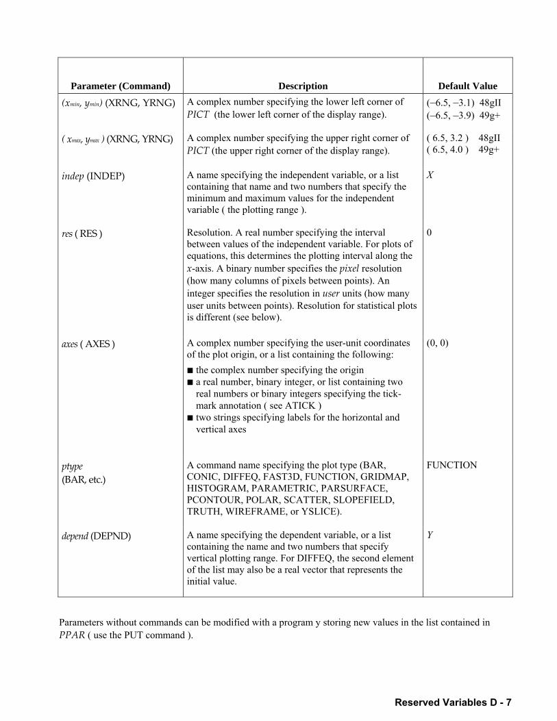
Reserved Variables D - 7
Parameter (Command) Description Default Value
(xmin, ymin) (XRNG, YRNG) A complex number specifying the lower left corner of PICT (the lower left corner of the display range).
(6.5, 3.1) 48gII (6.5, 3.9) 49g+
( xmax, ymax ) (XRNG, YRNG) A complex number specifying the upper right corner of PICT (the upper right corner of the display range).
( 6.5, 3.2 ) 48gII ( 6.5, 4.0 ) 49g+
indep (INDEP) A name specifying the independent variable, or a list containing that name and two numbers that specify the minimum and maximum values for the independent variable ( the plotting range ).
X
res ( RES ) Resolution. A real number specifying the interval between values of the independent variable. For plots of equations, this determines the plotting interval along the x-axis. A binary number specifies the pixel resolution (how many columns of pixels between points). An integer specifies the resolution in user units (how many user units between points). Resolution for statistical plots is different (see below).
0
axes ( AXES ) A complex number specifying the user-unit coordinates of the plot origin, or a list containing the following: ! the complex number specifying the origin ! a real number, binary integer, or list containing two
real numbers or binary integers specifying the tick-mark annotation ( see ATICK )
! two strings specifying labels for the horizontal and vertical axes
(0, 0)
ptype (BAR, etc.)
A command name specifying the plot type (BAR, CONIC, DIFFEQ, FAST3D, FUNCTION, GRIDMAP, HISTOGRAM, PARAMETRIC, PARSURFACE, PCONTOUR, POLAR, SCATTER, SLOPEFIELD, TRUTH, WIREFRAME, or YSLICE).
FUNCTION
depend (DEPND) A name specifying the dependent variable, or a list containing the name and two numbers that specify vertical plotting range. For DIFFEQ, the second element of the list may also be a real vector that represents the initial value.
Y
Parameters without commands can be modified with a program y storing new values in the list contained in PPAR ( use the PUT command ).
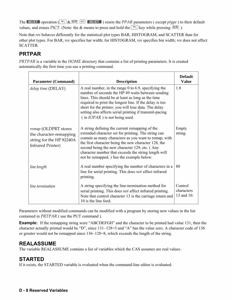
D - 8 Reserved Variables
The $RESET$ operation (&ôL %RESET% ) resets the PPAR parameters ( except ptype ) to their default values, and erases PICT. (Note: the & means to press and hold the key while pressing ô).
Note that res behaves differently for the statistical plot types BAR, HISTOGRAM, and SCATTER than for other plot types. For BAR, res specifies bar width; for HISTOGRAM, res specifies bin width; res does not affect SCATTER.
PRTPAR PRTPAR is a variable in the HOME directory that contains a list of printing parameters. It is created automatically the first time you use a printing command.
Parameter (Command) Description Default Value
delay time (DELAY) A real number, in the range 0 to 6.9, specifying the number of seconds the HP 49 waits between sending lines. This should be at least as long as the time required to print the longest line. If the delay is too short for the printer, you will lose data. The delay setting also affects serial printing if transmit-pacing ( in IOPAR ) is not being used.
1.8
remap (OLDPRT stores the character-remapping string for the HP 82240A Infrared Printer)
A string defining the current remapping of the extended character set for printing. The string can contain as many characters as you want to remap, with the first character being the new character 128, the second being the new character 129, etc. ( Any character number that exceeds the string length will not be remapped. ) See the example below.
Empty string.
line length A real number specifying the number of characters in a line for serial printing. This does not affect infrared printing.
80
line termination A string specifying the line-termination method for serial printing. This does not affect infrared printing. Note that control character 13 is the carriage return and 10 is the line feed.
Control characters 13 and 10.
Parameters without modified commands can be modified with a program by storing new values in the list contained in PRTPAR ( use the PUT command ). Example: If the remapping string were ABCDEFGH and the character to be printed had value 131, then the character actually printed would be D, since 131128=3 and A has the value zero. A character code of 136 or greater would not be remapped since 136128=8, which exceeds the length of the string.
REALASSUME The variable REALASSUME contains a list of variables which the CAS assumes are real values.
STARTED If it exists, the STARTED variable is evaluated when the command-line editor is evaluated.
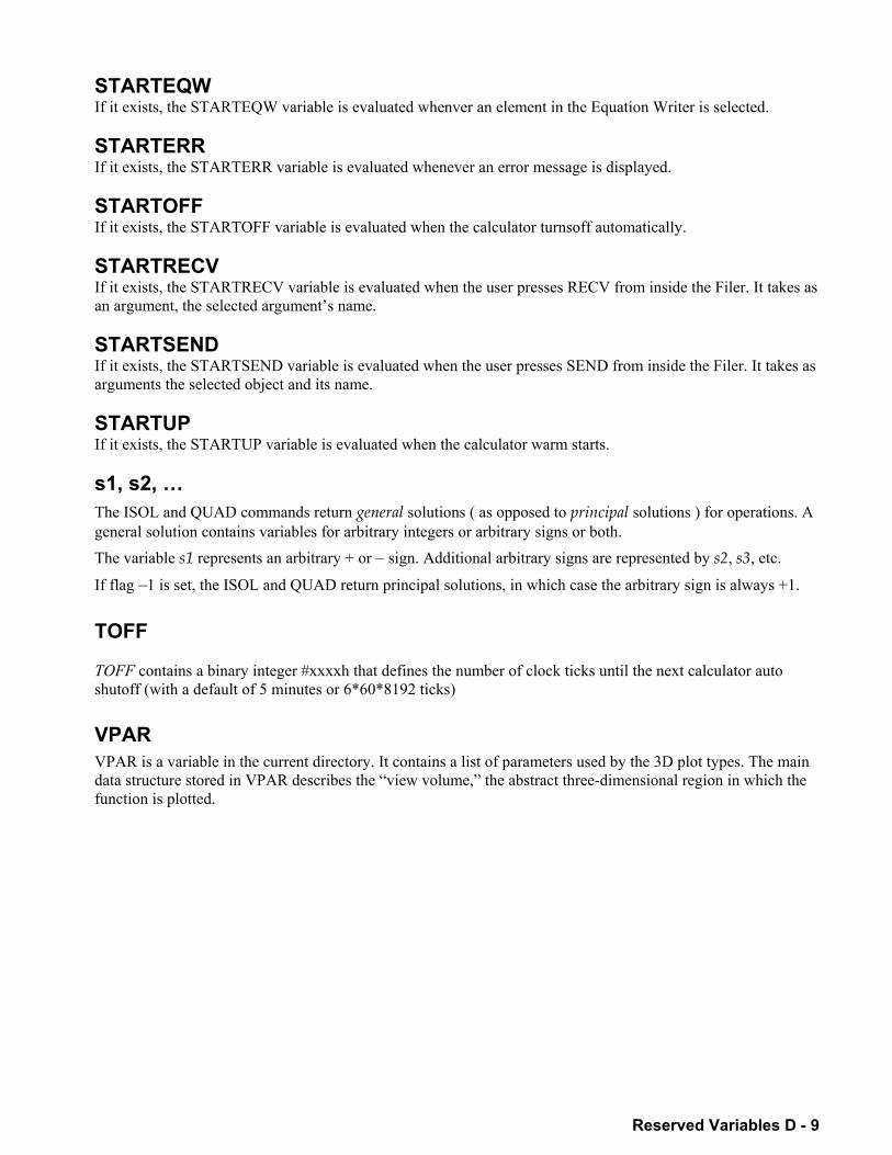
Reserved Variables D - 9
STARTEQW If it exists, the STARTEQW variable is evaluated whenver an element in the Equation Writer is selected.
STARTERR If it exists, the STARTERR variable is evaluated whenever an error message is displayed.
STARTOFF If it exists, the STARTOFF variable is evaluated when the calculator turnsoff automatically.
STARTRECV If it exists, the STARTRECV variable is evaluated when the user presses RECV from inside the Filer. It takes as an argument, the selected arguments name.
STARTSEND If it exists, the STARTSEND variable is evaluated when the user presses SEND from inside the Filer. It takes as arguments the selected object and its name.
STARTUP If it exists, the STARTUP variable is evaluated when the calculator warm starts.
s1, s2, The ISOL and QUAD commands return general solutions ( as opposed to principal solutions ) for operations. A general solution contains variables for arbitrary integers or arbitrary signs or both. The variable s1 represents an arbitrary + or sign. Additional arbitrary signs are represented by s2, s3, etc.
If flag 1 is set, the ISOL and QUAD return principal solutions, in which case the arbitrary sign is always +1. TOFF TOFF contains a binary integer #xxxxh that defines the number of clock ticks until the next calculator auto shutoff (with a default of 5 minutes or 6*60*8192 ticks) VPAR VPAR is a variable in the current directory. It contains a list of parameters used by the 3D plot types. The main data structure stored in VPAR describes the view volume, the abstract three-dimensional region in which the function is plotted.
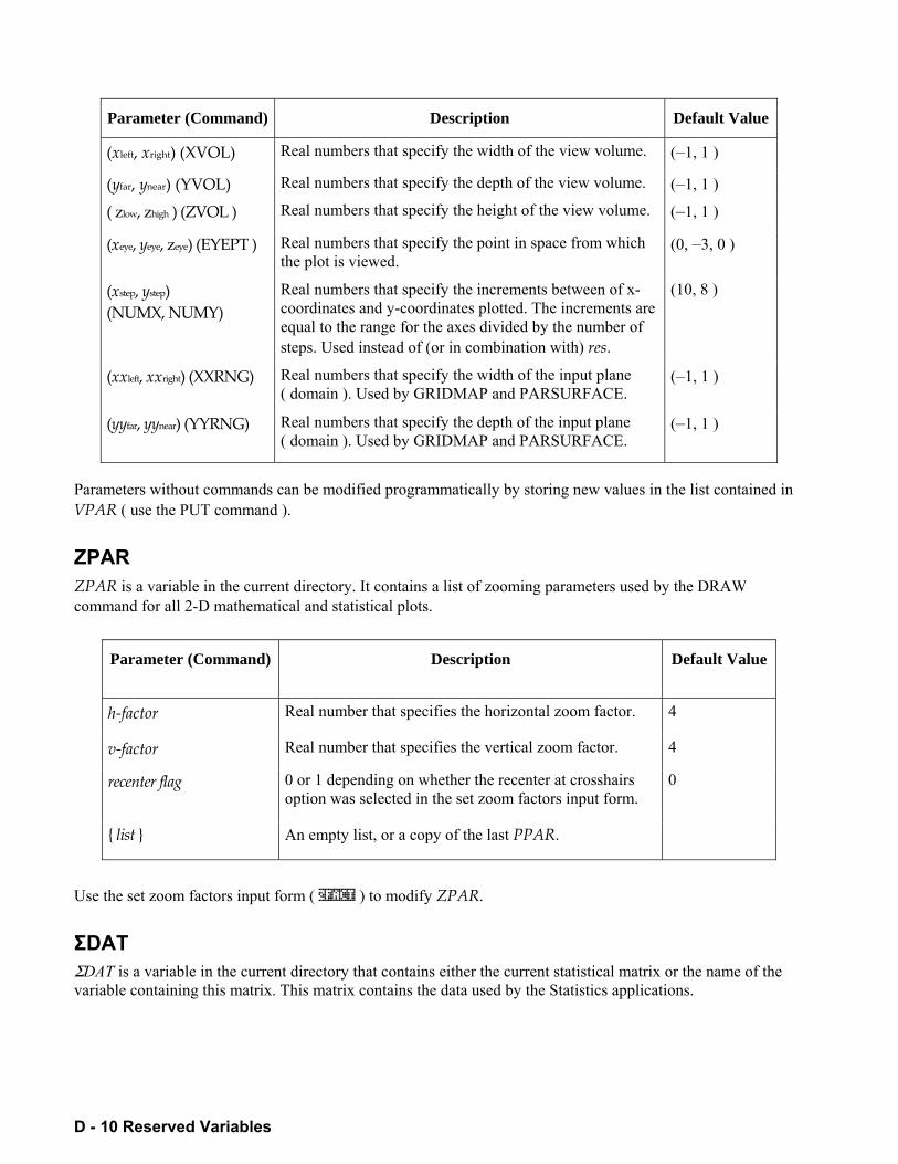
D - 10 Reserved Variables
Parameter (Command) Description Default Value
(xleft, xright) (XVOL) Real numbers that specify the width of the view volume. (1, 1 )
(yfar, ynear) (YVOL) Real numbers that specify the depth of the view volume. (1, 1 )
( zlow, zhigh ) (ZVOL ) Real numbers that specify the height of the view volume. (1, 1 )
(xeye, yeye, zeye) (EYEPT ) Real numbers that specify the point in space from which the plot is viewed.
(0, 3, 0 )
(xstep, ystep) (NUMX, NUMY)
Real numbers that specify the increments between of x-coordinates and y-coordinates plotted. The increments are equal to the range for the axes divided by the number of steps. Used instead of (or in combination with) res.
(10, 8 )
(xxleft, xxright) (XXRNG) Real numbers that specify the width of the input plane ( domain ). Used by GRIDMAP and PARSURFACE.
(1, 1 )
(yyfar, yynear) (YYRNG) Real numbers that specify the depth of the input plane ( domain ). Used by GRIDMAP and PARSURFACE.
(1, 1 )
Parameters without commands can be modified programmatically by storing new values in the list contained in VPAR ( use the PUT command ). ZPAR ZPAR is a variable in the current directory. It contains a list of zooming parameters used by the DRAW command for all 2-D mathematical and statistical plots.
Parameter (Command) Description Default Value
h-factor Real number that specifies the horizontal zoom factor. 4
v-factor Real number that specifies the vertical zoom factor. 4
recenter flag 0 or 1 depending on whether the recenter at crosshairs option was selected in the set zoom factors input form.
0
list An empty list, or a copy of the last PPAR.
Use the set zoom factors input form ( ZFACT ) to modify ZPAR. ΣDAT ΣDAT is a variable in the current directory that contains either the current statistical matrix or the name of the variable containing this matrix. This matrix contains the data used by the Statistics applications.
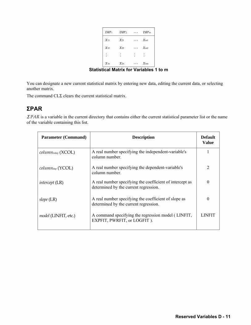
Reserved Variables D - 11
var1 var2 varm
x11 x21 xm1
x12 x22 xm2
x1n x2n xmn
Statistical Matrix for Variables 1 to m
You can designate a new current statistical matrix by entering new data, editing the current data, or selecting another matrix. The command CLΣ clears the current statistical matrix. ΣPAR Σ PAR is a variable in the current directory that contains either the current statistical parameter list or the name of the variable containing this list.
Parameter (Command) Description Default Value
columnindep (XCOL) A real number specifying the independent-variable's column number.
1
columndep (YCOL) A real number specifying the dependent-variable's column number.
2
intercept (LR) A real number specifying the coefficient of intercept as determined by the current regression.
0
slope (LR) A real number specifying the coefficient of slope as determined by the current regression.
0
model (LINFIT, etc.) A command specifying the regression model ( LINFIT, EXPFIT, PWRFIT, or LOGFIT ).
LINFIT

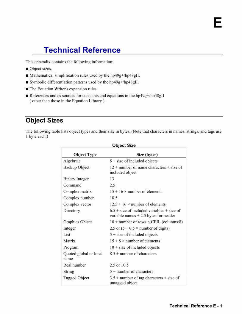
E
Technical Reference E - 1
11.Technical Reference This appendix contains the following information: ! Object sizes. ! Mathematical simplification rules used by the hp49g+/hp48gII. ! Symbolic differentiation patterns used by the hp49g+/hp48gII. ! The Equation Writer's expansion rules. ! References and as sources for constants and equations in the hp49g+/hp48gII
( other than those in the Equation Library ).
Object Sizes The following table lists object types and their size in bytes. (Note that characters in names, strings, and tags use 1 byte each.)
Object Size
Object Type Size (bytes) Algebraic 5 + size of included objects Backup Object 12 + number of name characters + size of
included object Binary Integer 13 Command 2.5 Complex matrix 15 + 16 × number of elements Complex number 18.5 Complex vector 12.5 + 16 × number of elements Directory 6.5 + size of included variables + size of
variable names + 2.5 bytes for header Graphics Object 10 + number of rows × CEIL (columns/8) Integer 2.5 or (5 + 0.5 × number of digits) List 5 + size of included objects Matrix 15 + 8 × number of elements Program 10 + size of included objects Quoted global or local name
8.5 + number of characters
Real number 2.5 or 10.5 String 5 + number of characters Tagged Object 3.5 + number of tag characters + size of
untagged object
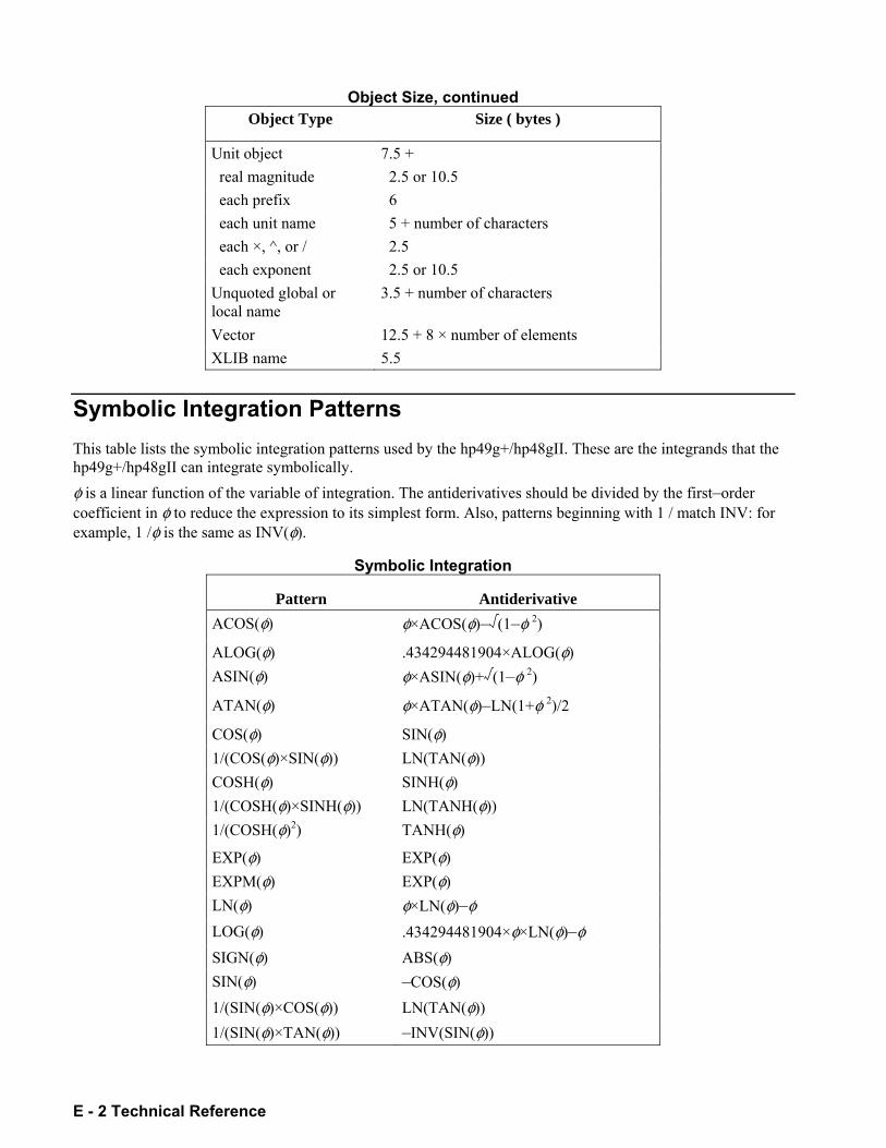
E - 2 Technical Reference
Object Size, continued Object Type Size ( bytes )
Unit object 7.5 + real magnitude 2.5 or 10.5 each prefix 6 each unit name 5 + number of characters each ×, ^, or / 2.5 each exponent 2.5 or 10.5 Unquoted global or local name
3.5 + number of characters
Vector 12.5 + 8 × number of elements XLIB name 5.5
Symbolic Integration Patterns This table lists the symbolic integration patterns used by the hp49g+/hp48gII. These are the integrands that the hp49g+/hp48gII can integrate symbolically. φ is a linear function of the variable of integration. The antiderivatives should be divided by the firstorder coefficient in φ to reduce the expression to its simplest form. Also, patterns beginning with 1 / match INV: for example, 1 /φ is the same as INV(φ).
Symbolic Integration
Pattern Antiderivative ACOS(φ) φ×ACOS(φ) (1φ 2)
ALOG(φ) .434294481904×ALOG(φ) ASIN(φ) φ×ASIN(φ)+ (1φ 2)
ATAN(φ) φ×ATAN(φ)LN(1+φ 2)/2
COS(φ) SIN(φ) 1/(COS(φ)×SIN(φ)) LN(TAN(φ)) COSH(φ) SINH(φ) 1/(COSH(φ)×SINH(φ)) LN(TANH(φ)) 1/(COSH(φ)2) TANH(φ)
EXP(φ) EXP(φ) EXPM(φ) EXP(φ) LN(φ) φ×LN(φ)φ LOG(φ) .434294481904×φ×LN(φ)φ SIGN(φ) ABS(φ) SIN(φ) COS(φ) 1/(SIN(φ)×COS(φ)) LN(TAN(φ)) 1/(SIN(φ)×TAN(φ)) INV(SIN(φ))

Technical Reference E - 3
Symbolic Integration (continued)
Pattern Antiderivative 1/(SIN(φ)×TAN(φ)) INV(SIN(φ))
1/(SIN(φ)2) INV(TAN(φ)) SINH(φ) COSH(φ) 1/(SINH(φ)×COSH(φ)) LN(TANH(φ)) 1/(SINH(φ)×TANH(φ)) INV(SINH(φ))
SQ(φ) φ 3/3
TAN(φ)2 TAN(φ)φ
TAN(φ) LN(COS(φ)) TAN(φ)/COS(φ) INV(COS(φ)) 1/TAN(φ) LN(SIN(φ)) 1/TAN(φ)×SIN(φ)) INV(SIN(φ)) TANH(φ) LN(COSH(φ)) TANH(φ)/COSH(φ) INV(COSH(φ)) 1/TANH(φ) LN(SINH(φ)) 1/TANH(φ)×SINH(φ)) INV(SINH(φ))
φ 2×φ 1.5/3 1/ φ 2× φ 1/(2× (φ)) 2× (φ)×.5
φ z(z symbolic) IFTE(z = = 1,LN(φ),φ (z+1)/(z+1))
φ z(z real, ≠0,1) φ (z+1)/(z+1)
φ 0 φ
φ 1 LN(φ)
1/φ LN(φ)
1/(1φ 2) ATANH(φ)
1/(1+φ 2) ATAN(φ)
1/(φ 2+1) ATAN(φ)
1/( (φ1)× (φ+1)) ACOSH(φ)
1/ (1φ 2) ASIN(φ)
1/ (1+φ 2) ASINH(φ)
1/ (φ 2+1) ASINH(φ)
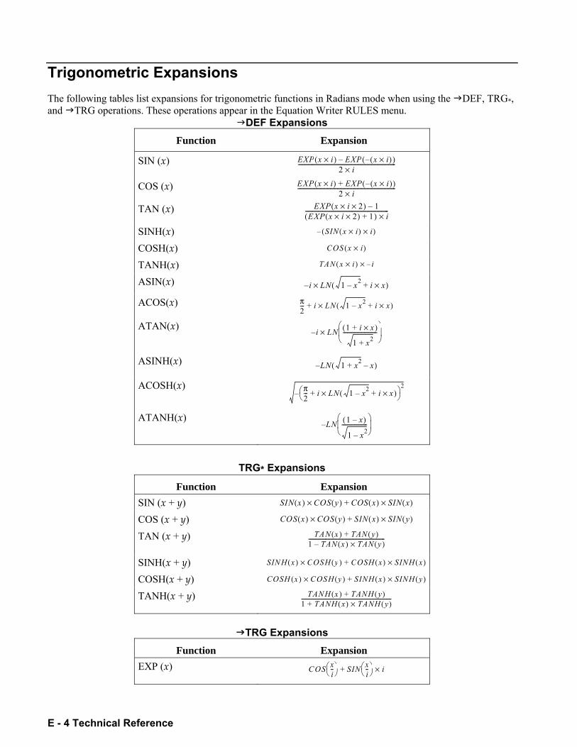
E - 4 Technical Reference
Trigonometric Expansions The following tables list expansions for trigonometric functions in Radians mode when using the "DEF, TRG*, and "TRG operations. These operations appear in the Equation Writer RULES menu.
"DEF Expansions Function Expansion
SIN (x) EXP x i×( ) EXP x i×( )( )2 i×
---------------------------------------------------------------------
COS (x) EXP x i×( ) EXP x i×( )( )+2 i×
---------------------------------------------------------------------
TAN (x) EXP x i 2××( ) 1EXP x i 2××( ) 1+( ) i×
-----------------------------------------------------------
SINH(x) SIN x i×( ) i×( ) COSH(x) COS x i×( ) TANH(x) TAN x i×( ) i× ASIN(x) i LN 1 x2 i x×+( )× ACOS(x) π
2--- i LN 1 x2 i x×+( )×+
ATAN(x)
i LN 1 i x×+( )
1 x2+------------------------⎝ ⎠⎜ ⎟⎛ ⎞
×
ASINH(x) LN 1 x2+ x( ) ACOSH(x) π
2--- i LN 1 x2 i x×+( )×+⎝ ⎠⎛ ⎞
2
ATANH(x)
LN 1 x( )
1 x2------------------⎝ ⎠⎜ ⎟⎛ ⎞
TRG* Expansions
Function Expansion SIN (x + y) SIN x( ) COS y( )× COS x( ) SIN x( )×+ COS (x + y) COS x( ) COS y( )× SIN x( ) SIN y( )×+ TAN (x + y) TAN x( ) TAN y( )+
1 TAN x( ) TAN y( )×------------------------------------------------------
SINH(x + y) SINH x( ) COSH y( )× COSH x( ) SINH x( )×+ COSH(x + y) COSH x( ) COSH y( )× SINH x( ) SINH y( )×+ TANH(x + y) TANH x( ) TANH y( )+
1 TANH x( ) TANH y( )×+----------------------------------------------------------------
"TRG Expansions Function Expansion
EXP (x) COS xi--⎝ ⎠⎛ ⎞ SIN x
i--⎝ ⎠⎛ ⎞ i×+
Technical Reference E - 5
Source References The following references were used as sources for many of the constants and equations used in the hp49g+/hp48gII. ( See References in chapter 5, Equation Reference, for the references used as sources for the Equation Library. )
1. E.A. Mechtly. The International System of Units, Physical Constants and Conversion Factors, Second
Revision. National Aeronautics and Space Administration, Washington DC, 1973. 2. The American Heritage Dictionary. Houghton Mifflin Company, Boston, MA, 1979.
3. American National Standard Metric Practice ANSI/IEEE Std 268-1982. The Institute of Electrical and Electronics Engineers, Inc., New York, 1982.
4. ASTM Standard Practice for Use of the International System of Units (SI) E380-89a. American Society for Testing and Materials, Philadelphia, 1989.
5. Handbook of Chemistry and Physics, 64th Edition, 1983-1984. CRC Press, Inc, Boca Raton, FL, 1983.
6. International Standard publication No. ISO 31/l-1978 (E).
7. The International System of Units (SI), Fourth Edition. The National Bureau of Standards Special Publication 330, Washington D.C., 1981.
8. National Aerospace Standard. Aerospace Industries Association of America, Inc., Washington D.C., 1977.
9. Physics Letters B, vol 204, 14 April 1988 (ISSN 0370-2693).

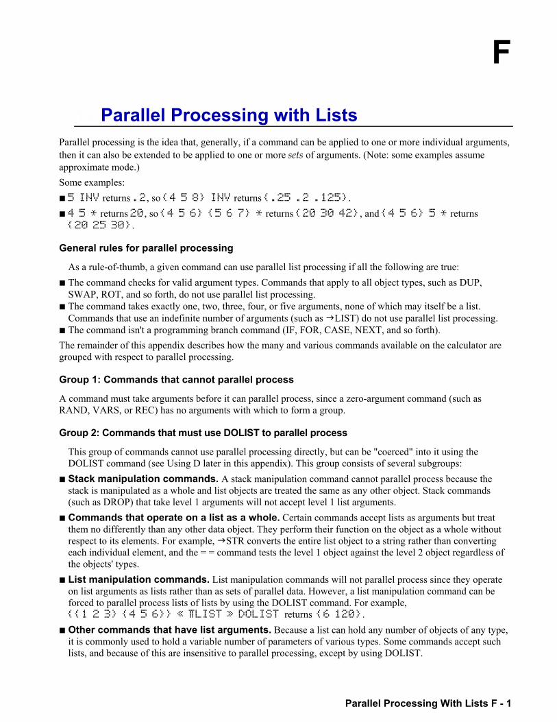
F
Parallel Processing With Lists F - 1
12.Parallel Processing with Lists Parallel processing is the idea that, generally, if a command can be applied to one or more individual arguments, then it can also be extended to be applied to one or more sets of arguments. (Note: some examples assume approximate mode.) Some examples: ! 5 INV returns .2, so 4 5 8 INV returns .25 .2 .125. ! 4 5 * returns 20, so 4 5 6 5 6 7 * returns 20 30 42, and 4 5 6 5 * returns
20 25 30.
General rules for parallel processing
As a rule-of-thumb, a given command can use parallel list processing if all the following are true: ! The command checks for valid argument types. Commands that apply to all object types, such as DUP,
SWAP, ROT, and so forth, do not use parallel list processing. ! The command takes exactly one, two, three, four, or five arguments, none of which may itself be a list.
Commands that use an indefinite number of arguments (such as "LIST) do not use parallel list processing. ! The command isn't a programming branch command (IF, FOR, CASE, NEXT, and so forth). The remainder of this appendix describes how the many and various commands available on the calculator are grouped with respect to parallel processing.
Group 1: Commands that cannot parallel process
A command must take arguments before it can parallel process, since a zero-argument command (such as RAND, VARS, or REC) has no arguments with which to form a group.
Group 2: Commands that must use DOLIST to parallel process
This group of commands cannot use parallel processing directly, but can be "coerced" into it using the DOLIST command (see Using D later in this appendix). This group consists of several subgroups:
! Stack manipulation commands. A stack manipulation command cannot parallel process because the stack is manipulated as a whole and list objects are treated the same as any other object. Stack commands (such as DROP) that take level 1 arguments will not accept level 1 list arguments.
! Commands that operate on a list as a whole. Certain commands accept lists as arguments but treat them no differently than any other data object. They perform their function on the object as a whole without respect to its elements. For example, "STR converts the entire list object to a string rather than converting each individual element, and the = = command tests the level 1 object against the level 2 object regardless of the objects' types.
! List manipulation commands. List manipulation commands will not parallel process since they operate on list arguments as lists rather than as sets of parallel data. However, a list manipulation command can be forced to parallel process lists of lists by using the DOLIST command. For example, 1 2 3 4 5 6 « œLIST » DOLIST returns 6 120.
! Other commands that have list arguments. Because a list can hold any number of objects of any type, it is commonly used to hold a variable number of parameters of various types. Some commands accept such lists, and because of this are insensitive to parallel processing, except by using DOLIST.
F - 2 Parallel Processing With Lists
! Index-oriented commands. Many array commands either establish the size of an array in rows and columns or manipulate individual elements by their row and column indices. These commands expect these row and column indices to be real number pairs collected in lists. For example, 3 4 RANM will generate a random integer matrix having 3 rows and 4 columns. Since these commands can normally use lists as arguments, they cannot perform parallel processing, except by using DOLIST.
! Program control commands. Program control structures and commands do no perform parallel processing and cannot be forced to do so. However, programs containing these structures can be made to parallel process by using DOLIST. For example, 1 2 3 4 5 6 1 « IF DUP 3 ‰ THEN DROP END » DOLIST returns 3 4 5 6.
Group 3: commands that sometimes work with parallel processing
! Graphics commands that can take pixel coordinates as arguments expect those coordinates to be presented as two-element lists of binary integers. Since these commands can normally use lists as arguments, they cannot parallel process, except by using DOLIST.
! For the two-argument graphics commands (BOX, LINE, TLINE), if either argument is not a list (a complex number, for example), then the commands will parallel process, taking the list argument to be multiple complex number coordinates. For example, (0,0) (1,1) (3,2) LINE will draw two lines between (0,0) and (1,1) and between (0,0) and (3,2).
Group 4: ADD and +
! On HP 48S and HP 48SX calculators, the + command has been used to append lists or to append elements to lists. Thus 1 2 3 4 + returns 1 2 3 4. With the advent of parallel processing in the hp 48g and hp49g series, the ADD command was created to perform parallel addition instead of +. This has several ramifications:
! To add two lists in parallel, you must do one of the following: " Use ADD from the !´%LIST% menu. " Create a custom menu containing the ADD command. " Assign the ADD command to a user-defined key.
! User programs must be written using ADD instead of + if the program is to be able to perform direct parallel processing, or written with + and applied to their arguments by using DOLIST. For example, programs such as « x 'x+2' » will produce list concatenation when x is a list rather than parallel addition, unless rewritten as « x 'x ADD 2' »
! Algebraic expressions capable of calculating with variables containing lists (including those intended to become user-defined functions) cannot be created in RPN syntax since using ADD to add two symbolic arguments concatenates the arguments with + rather than with ADD. For example, 'X' DUP 2 ^ SWAP 4 * ADD 'F(X)' SWAP = produces 'F(X)=X^2+4*X' rather than 'F(X)=X^2 ADD 4*X'.
Group 5: Commands that set modes / states
Commands that store values in system-specific locations so as to control certain modes and machine states can generally be used to parallel process data. The problem is that each successive parameter in the list cancels the setting established by the previous parameter. For example, 1 2 3 4 5 FIX is effectively the same as 5 FIX.
Group 6: One-argument, one-result commands
These commands are the easiest to use with parallel processing. Simply provide the command with a list of arguments instead of the expected single argument. Some examples:
1 -2 3 -4 ABS returns 1 2 3 4
Parallel Processing With Lists F - 3
DEG 0 30 60 90 SIN returns O. 5. 866025403784 1 1 A 'SIN(Z)' INV returns 1 'INV(A)' 'INV(SIN(Z))'
Group 7: Two -argument, one result commands
Two-argument commands can operate in parallel in any of three different ways: ! list list ! list object ! object list In the first form, parallel elements are combined by the command: 1 2 3 4 5 6 % returns .04 .1 .18 . In the second form, the level 1 object is combined with each element in the level 2 list in succession: 1 2 3 30 %CH returns 2900 1400 900. In the third form, the level 2 object is combined with each element of the level 1 list in succession: 50 1 2 3 % T returns 2 4 6 .
Group 8: Multiple-argument, one-result commands
Commands that take multiple (3, 4, or 5) arguments can perform parallel processing only if all arguments are lists. For example, 'SIN(X)' 'COS(X)' 'TAN(X)' X X X 0 0 0 ROOT returns 0 90 0. Notice that lists must be used even though the level 1 and level 2 lists each contain multiples of the same element.
Group 9: Multiple-result commands
Any command that allows parallel processing, but produces multiple results from its input data, will return its results as a single list. For example, 1 2 3 4 5 6 RC CR produces 1 4 2 5 3 6 rather than the more expected 1 2 3 4 5 6 . The following UNMIX program will unmix the data given the number of expected result lists: « OVER SIZE l n s « 1 n FOR j j s FOR i l i GET n STEP s n / LIST NEXT » »
Taking 1 4 2 5 3 6 from above as the result of C"R (a command which should return two results), 2 UNMIX gives 1 2 3 4 5 6 .
Group 10: Quirky commands
A few commands behave uniquely with respect to parallel processing: ! DELALARM. This command can take a list of arguments. Note, however, that deletions from early in the
alarm list will change the alarm indices of the later alarm entries. Thus, if there are only three alarms, 1 3 DELALARM will cause an error, whereas 3 1 DELALARM will not.
! DOERR. This command forces an error state that causes all running programs and commands to halt. Thus, even though providing the command with a list argument will cause the command to perform parallel processing, the first error state will cause the command to abort and none of the rest of the list arguments will be used.
! FREE, MERGE. These commands are for the HP 48GX and do not apply to the hp49g+/hp48gII.
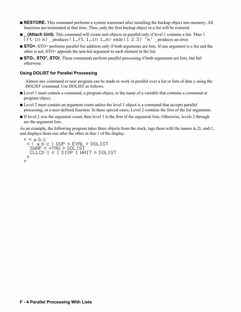
F - 4 Parallel Processing With Lists
! RESTORE. This command performs a system warmstart after installing the backup object into memory. All functions are terminated at that time. Thus, only the first backup object in a list will be restored.
! _ (Attach Unit). This command will create unit objects in parallel only if level 1 contains a list. Thus 1 ft in m _ produces 1_ft 1_in 1_m while 1 2 3 'm' _ produces an error.
! STO+. STO+ performs parallel list addition only if both arguments are lists. If one argument is a list and the other is not, STO+ appends the non-list argument to each element in the list.
! STO-, STO*, STO/. These commands perform parallel processing if both arguments are lists, but fail otherwise.
Using DOLIST for Parallel Processing
Almost any command or user program can be made to work in parallel over a list or lists of data y using the DOLIST command. Use DOLIST as follows.
! Level 1 must contain a command, a program object, or the name of a variable that contains a command or program object.
! Level 2 must contain an argument count unless the level 1 object is a command that accepts parallel processing, or a user-defined function. In these special cases, Level 2 contains the first of the list arguments.
! If level 2 was the argument count, then level 3 is the first of the argument lists. Otherwise, levels 2 through are the argument lists.
As an example, the following program takes three objects from the stack, tags them with the names a, b, and c, and displays them one after the other in line 1 of the display. « a b c « a b c DUP « EVAL » DOLIST SWAP « TAG » DOLIST CLLCD 1 « 1 DISP 1 WAIT » DOLIST » »
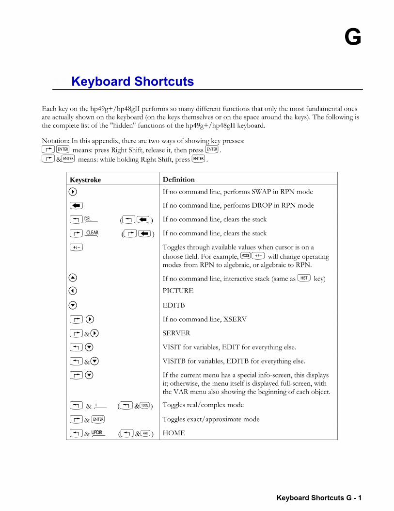
G
Keyboard Shortcuts G - 1
13.Keyboard Shortcuts
Each key on the hp49g+/hp48gII performs so many different functions that only the most fundamental ones are actually shown on the keyboard (on the keys themselves or on the space around the keys). The following is the complete list of the "hidden" functions of the hp49g+/hp48gII keyboard. Notation: In this appendix, there are two ways of showing key presses: @` means: press Right Shift, release it, then press `. @&` means: while holding Right Shift, press `.
Keystroke Definition
If no command line, performs SWAP in RPN mode
If no command line, performs DROP in RPN mode
!¶ (!) If no command line, clears the stack
@· (@) If no command line, clears the stack
W Toggles through available values when cursor is on a choose field. For example, HW will change operating modes from RPN to algebraic, or algebraic to RPN.
If no command line, interactive stack (same as M key)
PICTURE
EDITB
@ If no command line, XSERV
@& SERVER
! VISIT for variables, EDIT for everything else.
!& VISITB for variables, EDITB for everything else.
@ If the current menu has a special info-screen, this displays it; otherwise, the menu itself is displayed full-screen, with the VAR menu also showing the beginning of each object.
! & ¥ (!&I) Toggles real/complex mode
@& ` Toggles exact/approximate mode
!& § (!&J) HOME
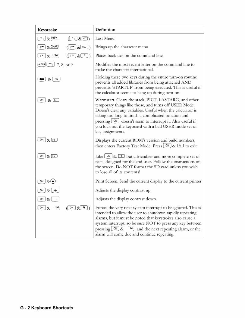
G - 2 Keyboard Shortcuts
Keystroke Definition
!& « (!&L) Last Menu
@&± (@&N) Brings up the character menu
@&³ (@&O) Places back-tics on the command line
~! 7, 8, or 9 Modifies the most recent letter on the command line to make the character international.
& $ Holding these two keys during the entire turn-on routine prevents all added libraries from being attached AND prevents 'STARTUP' from being executed. This is useful if the calculator seems to hang up during turn-on.
$ & C Warmstart. Clears the stack, PICT, LASTARG, and other temporary things like those, and turns off USER Mode. Doesn't clear any variables. Useful when the calculator is taking too long to finish a complicated function and pressing $ doesn't seem to interrupt it. Also useful if you lock out the keyboard with a bad USER mode set of key assignments.
$& D Displays the current ROM's version and build numbers, then enters Factory Test Mode. Press $& C to exit
$& F Like $& D but a friendlier and more complete set of tests, designed for the end-user. Follow the instructions on the screen. Do NOT format the SD card unless you wish to lose all of its contents!
$& Print Screen. Send the current display to the current printer
$& + Adjusts the display contrast up.
$& - Adjusts the display contrast down.
$& Ó ($&9) Forces the very next system interrupt to be ignored. This is intended to allow the user to shutdown rapidly repeating alarms, but it must be noted that keystrokes also cause a system interrupt, so be sure NOT to press any key between pressing $& Ó and the next repeating alarm, or the alarm will come due and continue repeating.
Keyboard Shortcuts G - 3
Press and Hold key combinations The table below indicates the function performed by pressing and holding two keys at the same time. The shift key listed is pressed first and while that key is still being held down, the second key listed is pressed.
Keycode Keystroke Definition 11.21 through 16.21
! & A through F Accesses the graphing input forms
22.21 ! & £ (!& H) MODES menu (menu 63)
23.21 ! & ¥ (!& I) Real/Complex toggle (flag -103)
31.21 ! & § (!& J) HOME
33.21 ! & « (!& L) Last Menu
35.21 ! & VISITB/EDITB (instead of VISIT/EDIT)
36.31 @ & SERVER (if no command line)
42.31 @ & ± (@& N) CHARS menu (menu 62)
43.31 @ & O ` `
72.31 @ & Ï (@& 7) Solver menu (menu 74)
74.31 @ & Ó (@& 9) TIME menu (menu 167)
104.31 @ & í (@& ) ; or . (depends on flag -51)
105.31 @ & ï (@& `) Exact/Approx toggle (flag -105)
43.61 ~@& O (omega)
84.61 ~@& 6 °(degree symbol)
93.61 ~@& 2 ¡(upside down exclamation point)
94.61 ~@& 3 ¿ (upside down question mark)
104.61 ~@&í(@&) ; or . (depends on flag -51)
Shifted softkeys This section describes the effect of using the shift keys and menu labels displayed above the A through F keys. @%VARNAME% = 'varname' !©. Applies to the VAR menu, CUSTOM menus obtained by pressing !£, or via the programmable MENU or TMENU commands, and any menu containing a variable (e.g. pressing @%EQ% in the ROOT menu [menu number 75] yields 'EQ' !©even in program mode.)
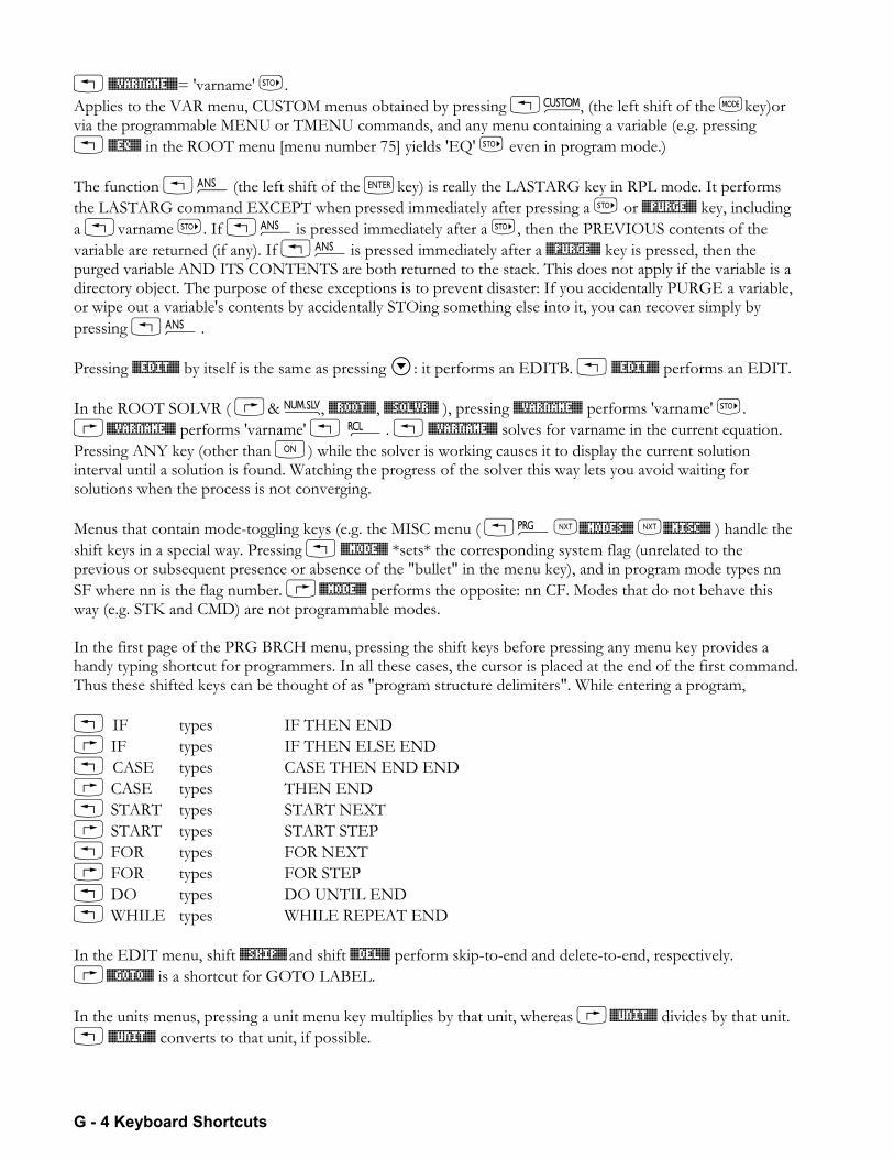
G - 4 Keyboard Shortcuts
! %VARNAME%= 'varname' . Applies to the VAR menu, CUSTOM menus obtained by pressing !£, (the left shift of the Hkey)or via the programmable MENU or TMENU commands, and any menu containing a variable (e.g. pressing ! %EQ% in the ROOT menu [menu number 75] yields 'EQ' even in program mode.) The function !î(the left shift of the `key) is really the LASTARG key in RPL mode. It performs the LASTARG command EXCEPT when pressed immediately after pressing a or %PURGE% key, including a !varname . If !îis pressed immediately after a , then the PREVIOUS contents of the variable are returned (if any). If !îis pressed immediately after a %PURGE% key is pressed, then the purged variable AND ITS CONTENTS are both returned to the stack. This does not apply if the variable is a directory object. The purpose of these exceptions is to prevent disaster: If you accidentally PURGE a variable, or wipe out a variable's contents by accidentally STOing something else into it, you can recover simply by pressing !î. Pressing %EDIT% by itself is the same as pressing : it performs an EDITB. ! %EDIT% performs an EDIT. In the ROOT SOLVR ( @& Ï, %ROOT%, %SOLVR% ), pressing %VARNAME% performs 'varname' K. @%VARNAME% performs 'varname' ! ©. ! %VARNAME% solves for varname in the current equation. Pressing ANY key (other than $) while the solver is working causes it to display the current solution interval until a solution is found. Watching the progress of the solver this way lets you avoid waiting for solutions when the process is not converging. Menus that contain mode-toggling keys (e.g. the MISC menu ( !°L%MODES% L%MISC% ) handle the shift keys in a special way. Pressing ! %MODE% *sets* the corresponding system flag (unrelated to the previous or subsequent presence or absence of the "bullet" in the menu key), and in program mode types nn SF where nn is the flag number. @%MODE% performs the opposite: nn CF. Modes that do not behave this way (e.g. STK and CMD) are not programmable modes. In the first page of the PRG BRCH menu, pressing the shift keys before pressing any menu key provides a handy typing shortcut for programmers. In all these cases, the cursor is placed at the end of the first command. Thus these shifted keys can be thought of as "program structure delimiters". While entering a program, ! IF types IF THEN END @ IF types IF THEN ELSE END ! CASE types CASE THEN END END @ CASE types THEN END ! START types START NEXT @ START types START STEP ! FOR types FOR NEXT @ FOR types FOR STEP ! DO types DO UNTIL END ! WHILE types WHILE REPEAT END In the EDIT menu, shift %SKIP% and shift %DEL% perform skip-to-end and delete-to-end, respectively. @%GOTO% is a shortcut for GOTO LABEL. In the units menus, pressing a unit menu key multiplies by that unit, whereas @%UNIT% divides by that unit. ! %UNIT% converts to that unit, if possible.
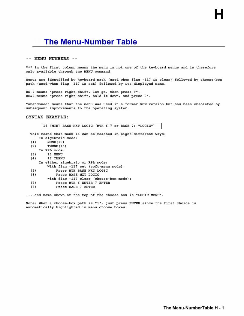
H
The Menu-NumberTable H - 1
14.The Menu-Number Table
-- MENU NUMBERS -- "*" in the first column means the menu is not one of the keyboard menus and is therefore only available through the MENU command. Menus are identified by keyboard path (used when flag -117 is clear) followed by choose-box path (used when flag -117 is set) followed by its displayed name. RS-9 means "press right-shift, let go, then press 9". RS&9 means "press right-shift, hold it down, and press 9". "Abandoned" means that the menu was used in a former ROM version but has been obsoleted by subsequent improvements to the operating system.
SYNTAX EXAMPLE: 16 [MTH] BASE NXT LOGIC (MTH 6 7 or BASE 7: "LOGIC") This means that menu 16 can be reached in eight different ways: In algebraic mode: (1) MENU(16) (2) TMENU(16) In RPL mode: (3) 16 MENU (4) 16 TMENU In either algebraic or RPL mode: With flag -117 set (soft-menu mode): (5) Press MTH BASE NXT LOGIC (6) Press BASE NXT LOGIC With flag -117 clear (choose-box mode): (7) Press MTH 6 ENTER 7 ENTER (8) Press BASE 7 ENTER ... and name shown at the top of the choose box is "LOGIC MENU". Note: When a choose-box path is "1", just press ENTER since the first choice is automatically highlighted in menu choose boxes.
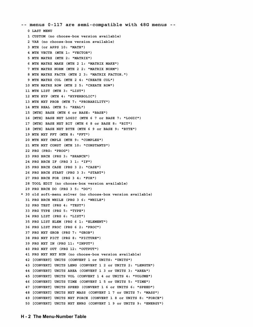
H - 2 The Menu-Number Table
-- menus 0-117 are semi-compatible with 48G menus -- 0 LAST MENU
1 CUSTOM (no choose-box version available)
2 VAR (no choose-box version available)
3 MTH (or APPS 10: "MATH")
4 MTH VECTR (MTH 1: "VECTOR")
5 MTH MATRX (MTH 2: "MATRIX")
6 MTH MATRX MAKE (MTH 2 1: "MATRIX MAKE")
7 MTH MATRX NORM (MTH 2 2: "MATRIX NORM")
8 MTH MATRX FACTR (MTH 2 3: "MATRIX FACTOR.")
9 MTH MATRX COL (MTH 2 4: "CREATE COL")
10 MTH MATRX ROW (MTH 2 5: "CREATE ROW")
11 MTH LIST (MTH 3: "LIST")
12 MTH HYP (MTH 4: "HYPERBOLIC")
13 MTH NXT PROB (MTH 7: "PROBABILITY")
14 MTH REAL (MTH 5: "REAL")
15 [MTH] BASE (MTH 6 or BASE: "BASE")
16 [MTH] BASE NXT LOGIC (MTH 6 7 or BASE 7: "LOGIC")
17 [MTH] BASE NXT BIT (MTH 6 8 or BASE 8: "BIT")
18 [MTH] BASE NXT BYTE (MTH 6 9 or BASE 9: "BYTE")
19 MTH NXT FFT (MTH 8: "FFT")
20 MTH NXT CMPLX (MTH 9: "COMPLEX")
21 MTH NXT CONST (MTH 10: "CONSTANTS")
22 PRG (PRG: "PROG")
23 PRG BRCH (PRG 3: "BRANCH")
24 PRG BRCH IF (PRG 3 1: "IF")
25 PRG BRCH CASE (PRG 3 2: "CASE")
26 PRG BRCH START (PRG 3 3: "START")
27 PRG BRCH FOR (PRG 3 4: "FOR")
28 TOOL EDIT (no choose-box version available)
29 PRG BRCH DO (PRG 3 5: "DO")
* 30 old soft-menu solver (no choose-box version available)
31 PRG BRCH WHILE (PRG 3 6: "WHILE")
32 PRG TEST (PRG 4: "TEST")
33 PRG TYPE (PRG 5: "TYPE")
34 PRG LIST (PRG 6: "LIST")
35 PRG LIST ELEM (PRG 6 1: "ELEMENT")
36 PRG LIST PROC (PRG 6 2: "PROC")
37 PRG NXT GROB (PRG 7: "GROB")
38 PRG NXT PICT (PRG 8: "PICTURE")
39 PRG NXT IN (PRG 11: "INPUT")
40 PRG NXT OUT (PRG 12: "OUTPUT")
41 PRG NXT NXT RUN (no choose-box version available)
42 [CONVERT] UNITS (CONVERT 1 or UNITS: "UNITS")
43 [CONVERT] UNITS LENG (CONVERT 1 2 or UNITS 2: "LENGTH")
44 [CONVERT] UNITS AREA (CONVERT 1 3 or UNITS 3: "AREA")
45 [CONVERT] UNITS VOL (CONVERT 1 4 or UNITS 4: "VOLUME")
46 [CONVERT] UNITS TIME (CONVERT 1 5 or UNITS 5: "TIME")
47 [CONVERT] UNITS SPEED (CONVERT 1 6 or UNITS 6: "SPEED")
48 [CONVERT] UNITS NXT MASS (CONVERT 1 7 or UNITS 7: "MASS")
49 [CONVERT] UNITS NXT FORCE (CONVERT 1 8 or UNITS 8: "FORCE")
50 [CONVERT] UNITS NXT ENRG (CONVERT 1 9 or UNITS 9: "ENERGY")
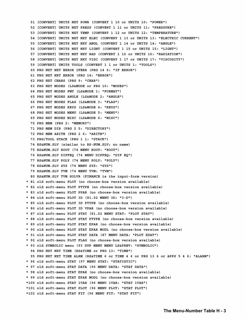
The Menu-Number Table H - 3
51 [CONVERT] UNITS NXT POWR (CONVERT 1 10 or UNITS 10: "POWER")
52 [CONVERT] UNITS NXT PRESS (CONVERT 1 11 or UNITS 11: "PRESSURE")
53 [CONVERT] UNITS NXT TEMP (CONVERT 1 12 or UNITS 12: "TEMPERATURE")
54 [CONVERT] UNITS NXT NXT ELEC (CONVERT 1 13 or UNITS 13: "ELECTRIC CURRENT")
55 [CONVERT] UNITS NXT NXT ANGL (CONVERT 1 14 or UNITS 14: "ANGLE")
56 [CONVERT] UNITS NXT NXT LIGHT (CONVERT 1 15 or UNITS 15: "LIGHT")
57 [CONVERT] UNITS NXT NXT RAD (CONVERT 1 16 or UNITS 16: "RADIATION")
58 [CONVERT] UNITS NXT NXT VISC (CONVERT 1 17 or UNITS 17: "VISCOSITY")
59 [CONVERT] UNITS TOOLS (CONVERT 1 1 or UNITS 1: "TOOLS")
60 PRG NXT NXT ERROR IFERR (PRG 14 6: "IF ERROR")
61 PRG NXT NXT ERROR (PRG 14: "ERROR")
62 PRG NXT CHARS (PRG 9: "CHAR")
63 PRG NXT MODES (LS&MODE or PRG 10: "MODES")
64 PRG NXT MODES FMT (LS&MODE 1: "FORMAT")
65 PRG NXT MODES ANGLE (LS&MODE 2: "ANGLE")
66 PRG NXT MODES FLAG (LS&MODE 3: "FLAG")
67 PRG NXT MODES KEYS (LS&MODE 4: "KEYS")
68 PRG NXT MODES MENU (LS&MODE 5: "MENU")
69 PRG NXT MODES MISC (LS&MODE 6: "MISC")
70 PRG MEM (PRG 2: "MEMORY")
71 PRG MEM DIR (PRG 2 5: "DIRECTORY")
72 PRG MEM ARITH (PRG 2 6: "ARITH")
73 PRG/TOOL STACK (PRG 1 1: "STACK")
74 RS&NUM.SLV (similar to RS-NUM.SLV; no name)
75 RS&NUM.SLV ROOT (74 MENU ROOT: "ROOT")
76 RS&NUM.SLV DIFFEQ (74 MENU DIFFEQ: "DIF EQ")
77 RS&NUM.SLV POLY (74 MENU POLY: "POLY")
78 RS&NUM.SLV SYS (74 MENU SYS: "SYS")
79 RS&NUM.SLV TVM (74 MENU TVM: "TVM")
80 RS&NUM.SLV TVM SOLVR (FINANCE is the input-form version)
* 81 old soft-menu PLOT (no choose-box version available)
* 82 old soft-menu PLOT PTYPE (no choose-box version available)
* 83 old soft-menu PLOT PPAR (no choose-box version available)
* 84 old soft-menu PLOT 3D (81.02 MENU 3D: "3-D")
* 85 old soft-menu PLOT 3D PTYPE (no choose-box version available)
* 86 old soft-menu PLOT 3D VPAR (no choose-box version available)
* 87 old soft-menu PLOT STAT (81.02 MENU STAT: "PLOT STAT")
* 88 old soft-menu PLOT STAT PTYPE (no choose-box version available)
* 89 old soft-menu PLOT STAT ΣPAR (no choose-box version available) * 90 old soft-menu PLOT STAT ΣPAR MODL (no choose-box version available) * 91 old soft-menu PLOT STAT DATA (87 MENU DATA: "PLOT ΣDAT") * 92 old soft-menu PLOT FLAG (no choose-box version available)
* 93 old SYMBOLIC menu (93 DUP MENU MENU LS&PREV: "SYMBOLIC")
94 PRG NXT NXT TIME (RS&TIME or PRG 13: "TIME")
95 PRG NXT NXT TIME ALRM (RS&TIME 6 or TIME 4 6 or PRG 13 6 or APPS 5 4 6: "ALARM")
* 96 old soft-menu STAT (97 MENU STAT: "STATISTIC")
* 97 old soft-menu STAT DATA (96 MENU DATA: "STAT DATA")
* 98 old soft-menu STAT ΣPAR (no choose-box version available) * 99 old soft-menu STAT ΣPAR MODL (no choose-box version available) *100 old soft-menu STAT 1VAR (96 MENU 1VAR: "STAT 1VAR")
*101 old soft-menu STAT PLOT (96 MENU PLOT: "STAT PLOT")
*102 old soft-menu STAT FIT (96 MENU FIT: "STAT FIT")
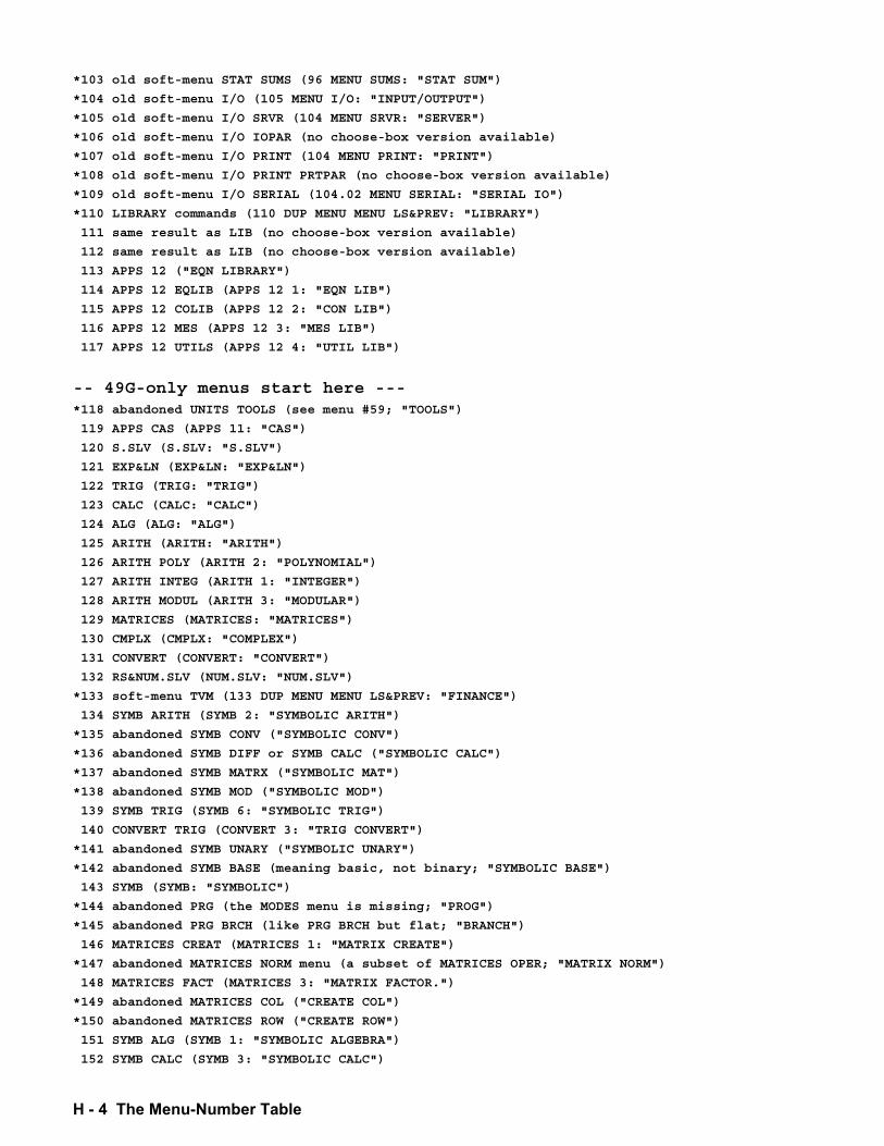
H - 4 The Menu-Number Table
*103 old soft-menu STAT SUMS (96 MENU SUMS: "STAT SUM")
*104 old soft-menu I/O (105 MENU I/O: "INPUT/OUTPUT")
*105 old soft-menu I/O SRVR (104 MENU SRVR: "SERVER")
*106 old soft-menu I/O IOPAR (no choose-box version available)
*107 old soft-menu I/O PRINT (104 MENU PRINT: "PRINT")
*108 old soft-menu I/O PRINT PRTPAR (no choose-box version available)
*109 old soft-menu I/O SERIAL (104.02 MENU SERIAL: "SERIAL IO")
*110 LIBRARY commands (110 DUP MENU MENU LS&PREV: "LIBRARY")
111 same result as LIB (no choose-box version available)
112 same result as LIB (no choose-box version available)
113 APPS 12 ("EQN LIBRARY")
114 APPS 12 EQLIB (APPS 12 1: "EQN LIB")
115 APPS 12 COLIB (APPS 12 2: "CON LIB")
116 APPS 12 MES (APPS 12 3: "MES LIB")
117 APPS 12 UTILS (APPS 12 4: "UTIL LIB")
-- 49G-only menus start here --- *118 abandoned UNITS TOOLS (see menu #59; "TOOLS")
119 APPS CAS (APPS 11: "CAS")
120 S.SLV (S.SLV: "S.SLV")
121 EXP&LN (EXP&LN: "EXP&LN")
122 TRIG (TRIG: "TRIG")
123 CALC (CALC: "CALC")
124 ALG (ALG: "ALG")
125 ARITH (ARITH: "ARITH")
126 ARITH POLY (ARITH 2: "POLYNOMIAL")
127 ARITH INTEG (ARITH 1: "INTEGER")
128 ARITH MODUL (ARITH 3: "MODULAR")
129 MATRICES (MATRICES: "MATRICES")
130 CMPLX (CMPLX: "COMPLEX")
131 CONVERT (CONVERT: "CONVERT")
132 RS&NUM.SLV (NUM.SLV: "NUM.SLV")
*133 soft-menu TVM (133 DUP MENU MENU LS&PREV: "FINANCE")
134 SYMB ARITH (SYMB 2: "SYMBOLIC ARITH")
*135 abandoned SYMB CONV ("SYMBOLIC CONV")
*136 abandoned SYMB DIFF or SYMB CALC ("SYMBOLIC CALC")
*137 abandoned SYMB MATRX ("SYMBOLIC MAT")
*138 abandoned SYMB MOD ("SYMBOLIC MOD")
139 SYMB TRIG (SYMB 6: "SYMBOLIC TRIG")
140 CONVERT TRIG (CONVERT 3: "TRIG CONVERT")
*141 abandoned SYMB UNARY ("SYMBOLIC UNARY")
*142 abandoned SYMB BASE (meaning basic, not binary; "SYMBOLIC BASE")
143 SYMB (SYMB: "SYMBOLIC")
*144 abandoned PRG (the MODES menu is missing; "PROG")
*145 abandoned PRG BRCH (like PRG BRCH but flat; "BRANCH")
146 MATRICES CREAT (MATRICES 1: "MATRIX CREATE")
*147 abandoned MATRICES NORM menu (a subset of MATRICES OPER; "MATRIX NORM")
148 MATRICES FACT (MATRICES 3: "MATRIX FACTOR.")
*149 abandoned MATRICES COL ("CREATE COL")
*150 abandoned MATRICES ROW ("CREATE ROW")
151 SYMB ALG (SYMB 1: "SYMBOLIC ALGEBRA")
152 SYMB CALC (SYMB 3: "SYMBOLIC CALC")
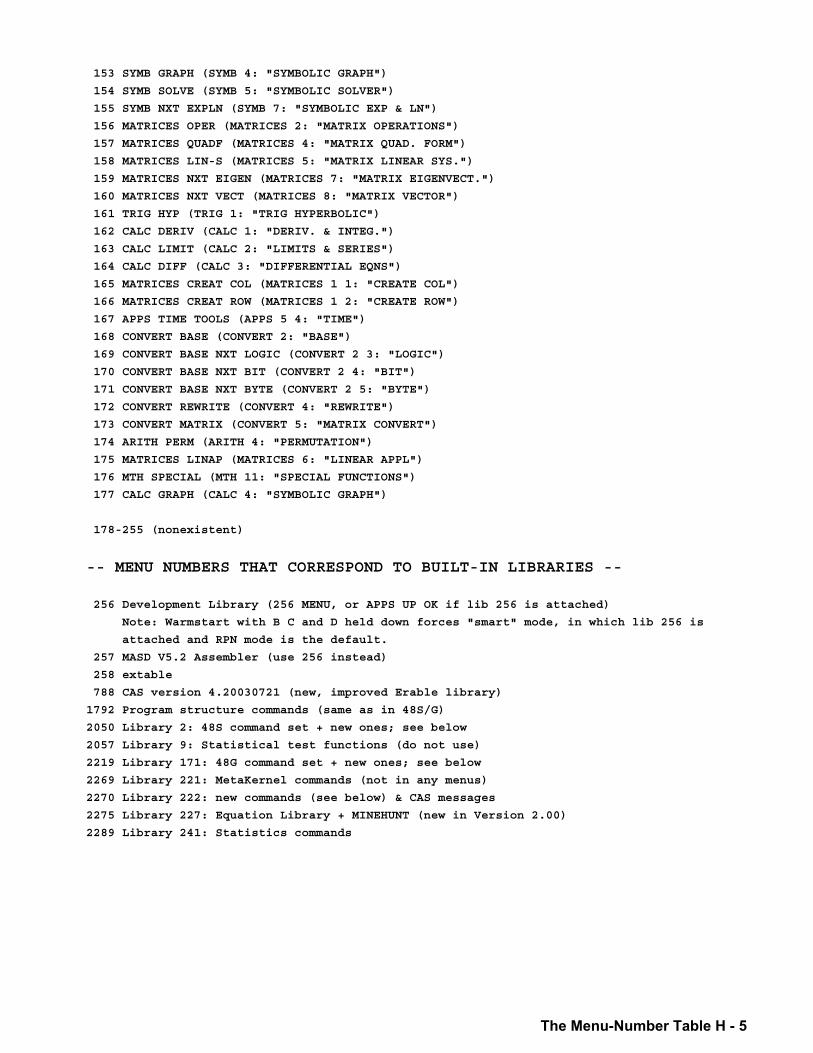
The Menu-Number Table H - 5
153 SYMB GRAPH (SYMB 4: "SYMBOLIC GRAPH")
154 SYMB SOLVE (SYMB 5: "SYMBOLIC SOLVER")
155 SYMB NXT EXPLN (SYMB 7: "SYMBOLIC EXP & LN")
156 MATRICES OPER (MATRICES 2: "MATRIX OPERATIONS")
157 MATRICES QUADF (MATRICES 4: "MATRIX QUAD. FORM")
158 MATRICES LIN-S (MATRICES 5: "MATRIX LINEAR SYS.")
159 MATRICES NXT EIGEN (MATRICES 7: "MATRIX EIGENVECT.")
160 MATRICES NXT VECT (MATRICES 8: "MATRIX VECTOR")
161 TRIG HYP (TRIG 1: "TRIG HYPERBOLIC")
162 CALC DERIV (CALC 1: "DERIV. & INTEG.")
163 CALC LIMIT (CALC 2: "LIMITS & SERIES")
164 CALC DIFF (CALC 3: "DIFFERENTIAL EQNS")
165 MATRICES CREAT COL (MATRICES 1 1: "CREATE COL")
166 MATRICES CREAT ROW (MATRICES 1 2: "CREATE ROW")
167 APPS TIME TOOLS (APPS 5 4: "TIME")
168 CONVERT BASE (CONVERT 2: "BASE")
169 CONVERT BASE NXT LOGIC (CONVERT 2 3: "LOGIC")
170 CONVERT BASE NXT BIT (CONVERT 2 4: "BIT")
171 CONVERT BASE NXT BYTE (CONVERT 2 5: "BYTE")
172 CONVERT REWRITE (CONVERT 4: "REWRITE")
173 CONVERT MATRIX (CONVERT 5: "MATRIX CONVERT")
174 ARITH PERM (ARITH 4: "PERMUTATION")
175 MATRICES LINAP (MATRICES 6: "LINEAR APPL")
176 MTH SPECIAL (MTH 11: "SPECIAL FUNCTIONS")
177 CALC GRAPH (CALC 4: "SYMBOLIC GRAPH")
178-255 (nonexistent)
-- MENU NUMBERS THAT CORRESPOND TO BUILT-IN LIBRARIES --
256 Development Library (256 MENU, or APPS UP OK if lib 256 is attached)
Note: Warmstart with B C and D held down forces "smart" mode, in which lib 256 is
attached and RPN mode is the default.
257 MASD V5.2 Assembler (use 256 instead)
258 extable
788 CAS version 4.20030721 (new, improved Erable library)
1792 Program structure commands (same as in 48S/G)
2050 Library 2: 48S command set + new ones; see below
2057 Library 9: Statistical test functions (do not use)
2219 Library 171: 48G command set + new ones; see below
2269 Library 221: MetaKernel commands (not in any menus)
2270 Library 222: new commands (see below) & CAS messages
2275 Library 227: Equation Library + MINEHUNT (new in Version 2.00)
2289 Library 241: Statistics commands
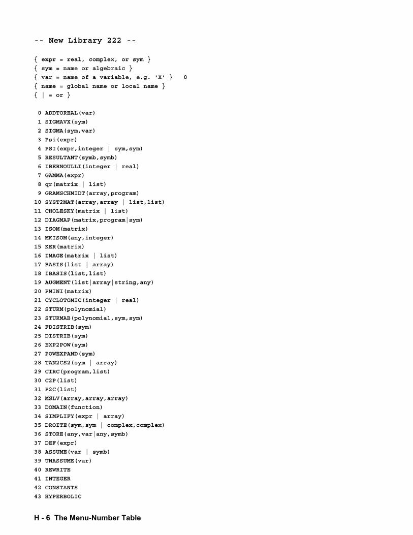
H - 6 The Menu-Number Table
-- New Library 222 --
expr = real, complex, or sym
sym = name or algebraic
var = name of a variable, e.g. 'X' 0
name = global name or local name
| = or
0 ADDTOREAL(var)
1 SIGMAVX(sym)
2 SIGMA(sym,var)
3 Psi(expr)
4 PSI(expr,integer | sym,sym)
5 RESULTANT(symb,symb)
6 IBERNOULLI(integer | real)
7 GAMMA(expr)
8 qr(matrix | list)
9 GRAMSCHMIDT(array,program)
10 SYST2MAT(array,array | list,list)
11 CHOLESKY(matrix | list)
12 DIAGMAP(matrix,program|sym)
13 ISOM(matrix)
14 MKISOM(any,integer)
15 KER(matrix)
16 IMAGE(matrix | list)
17 BASIS(list | array)
18 IBASIS(list,list)
19 AUGMENT(list|array|string,any)
20 PMINI(matrix)
21 CYCLOTOMIC(integer | real)
22 STURM(polynomial)
23 STURMAB(polynomial,sym,sym)
24 FDISTRIB(sym)
25 DISTRIB(sym)
26 EXP2POW(sym)
27 POWEXPAND(sym)
28 TAN2CS2(sym | array)
29 CIRC(program,list)
30 C2P(list)
31 P2C(list)
32 MSLV(array,array,array)
33 DOMAIN(function)
34 SIMPLIFY(expr | array)
35 DROITE(sym,sym | complex,complex)
36 STORE(any,var|any,symb)
37 DEF(expr)
38 ASSUME(var | symb)
39 UNASSUME(var)
40 REWRITE
41 INTEGER
42 CONSTANTS
43 HYPERBOLIC
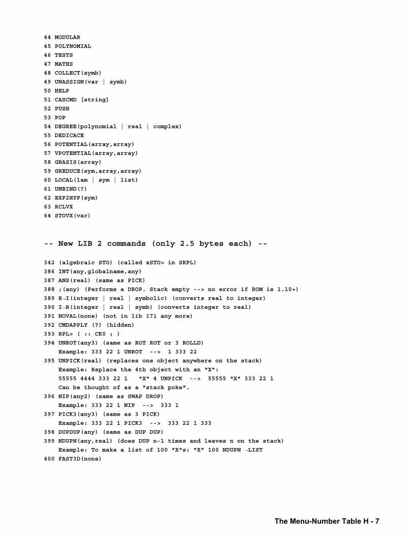
The Menu-Number Table H - 7
44 MODULAR
45 POLYNOMIAL
46 TESTS
47 MATHS
48 COLLECT(symb)
49 UNASSIGN(var | symb)
50 HELP
51 CASCMD [string]
52 PUSH
53 POP
54 DEGREE(polynomial | real | complex)
55 DEDICACE
56 POTENTIAL(array,array)
57 VPOTENTIAL(array,array)
58 GBASIS(array)
59 GREDUCE(sym,array,array)
60 LOCAL(lam | sym | list)
61 UNBIND(?)
62 EXP2HYP(sym)
63 RCLVX
64 STOVX(var)
-- New LIB 2 commands (only 2.5 bytes each) --
342 (algebraic STO) (called xSTO> in SRPL)
386 INT(any,globalname,any)
387 ANS(real) (same as PICK)
388 ;(any) (Performs a DROP. Stack empty --> no error if ROM is 1.10+)
389 R→I(integer | real | symbolic) (converts real to integer) 390 I→R(integer | real | symb) (converts integer to real) 391 NOVAL(none) (not in lib 171 any more)
392 CMDAPPLY (?) (hidden)
393 RPL> ( :: CK0 ; )
394 UNROT(any3) (same as ROT ROT or 3 ROLLD)
Example: 333 22 1 UNROT --> 1 333 22
395 UNPICK(real) (replaces one object anywhere on the stack)
Example: Replace the 4th object with an "X":
55555 4444 333 22 1 "X" 4 UNPICK --> 55555 "X" 333 22 1
Can be thought of as a "stack poke".
396 NIP(any2) (same as SWAP DROP)
Example: 333 22 1 NIP --> 333 1
397 PICK3(any3) (same as 3 PICK)
Example: 333 22 1 PICK3 --> 333 22 1 333
398 DUPDUP(any) (same as DUP DUP)
399 NDUPN(any,real) (does DUP n-1 times and leaves n on the stack)
Example: To make a list of 100 "X"s: "X" 100 NDUPN →LIST 400 FAST3D(none)
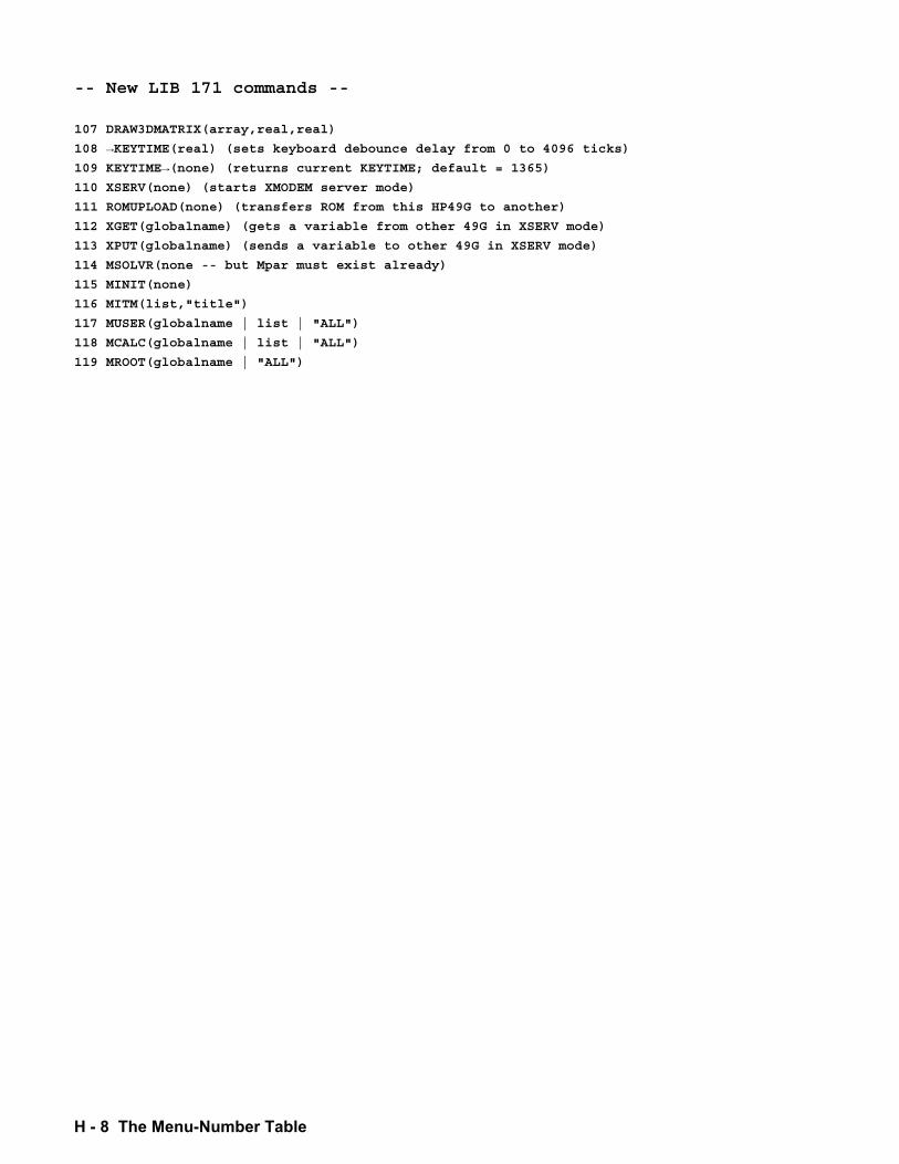
H - 8 The Menu-Number Table
-- New LIB 171 commands --
107 DRAW3DMATRIX(array,real,real)
108 →KEYTIME(real) (sets keyboard debounce delay from 0 to 4096 ticks) 109 KEYTIME→(none) (returns current KEYTIME; default = 1365) 110 XSERV(none) (starts XMODEM server mode)
111 ROMUPLOAD(none) (transfers ROM from this HP49G to another)
112 XGET(globalname) (gets a variable from other 49G in XSERV mode)
113 XPUT(globalname) (sends a variable to other 49G in XSERV mode)
114 MSOLVR(none -- but Mpar must exist already)
115 MINIT(none)
116 MITM(list,"title")
117 MUSER(globalname | list | "ALL")
118 MCALC(globalname | list | "ALL")
119 MROOT(globalname | "ALL")
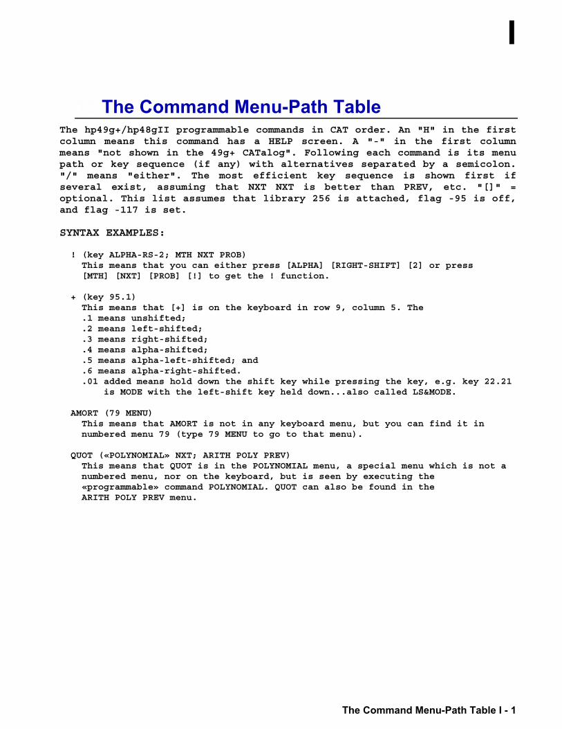
I
The Command Menu-Path Table I - 1
15.The Command Menu-Path Table The hp49g+/hp48gII programmable commands in CAT order. An "H" in the first column means this command has a HELP screen. A "-" in the first column means "not shown in the 49g+ CATalog". Following each command is its menu path or key sequence (if any) with alternatives separated by a semicolon. "/" means "either". The most efficient key sequence is shown first if several exist, assuming that NXT NXT is better than PREV, etc. "[]" = optional. This list assumes that library 256 is attached, flag -95 is off, and flag -117 is set. SYNTAX EXAMPLES: ! (key ALPHA-RS-2; MTH NXT PROB) This means that you can either press [ALPHA] [RIGHT-SHIFT] [2] or press [MTH] [NXT] [PROB] [!] to get the ! function. + (key 95.1) This means that [+] is on the keyboard in row 9, column 5. The .1 means unshifted; .2 means left-shifted; .3 means right-shifted; .4 means alpha-shifted; .5 means alpha-left-shifted; and .6 means alpha-right-shifted. .01 added means hold down the shift key while pressing the key, e.g. key 22.21 is MODE with the left-shift key held down...also called LS&MODE. AMORT (79 MENU) This means that AMORT is not in any keyboard menu, but you can find it in numbered menu 79 (type 79 MENU to go to that menu). QUOT («POLYNOMIAL» NXT; ARITH POLY PREV) This means that QUOT is in the POLYNOMIAL menu, a special menu which is not a numbered menu, nor on the keyboard, but is seen by executing the «programmable» command POLYNOMIAL. QUOT can also be found in the ARITH POLY PREV menu.
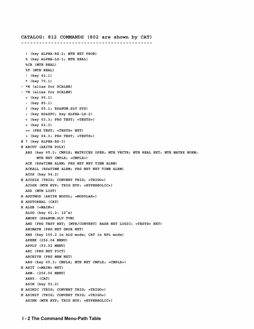
I - 2 The Command Menu-Path Table
CATALOG: 812 COMMANDS (802 are shown by CAT) --------------------------------------------
! (key ALPHA-RS-2; MTH NXT PROB)
% (key ALPHA-LS-1; MTH REAL)
%CH (MTH REAL)
%T (MTH REAL)
' (key 43.1)
* (key 75.1)
- *H (alias for SCALEH)
- *W (alias for SCALEW)
+ (key 95.1)
- (key 85.1)
/ (key 65.1; RS&NUM.SLV SYS)
; (key RS&SPC; key ALPHA-LS-2)
< (key 63.3; PRG TEST; «TESTS»)
= (key 62.3)
== (PRG TEST; «TESTS» NXT)
> (key 64.3; PRG TEST; «TESTS»)
H ? (key ALPHA-RS-3)
H ABCUV (ARITH POLY)
ABS (key 65.2; CMPLX; MATRICES OPER; MTH VECTR; MTH REAL NXT; MTH MATRX NORM;
MTH NXT CMPLX; «CMPLX»)
ACK (RS&TIME ALRM; PRG NXT NXT TIME ALRM)
ACKALL (RS&TIME ALRM; PRG NXT NXT TIME ALRM)
ACOS (key 54.2)
H ACOS2S (TRIG; CONVERT TRIG; «TRIGO»)
ACOSH (MTH HYP; TRIG HYP; «HYPERBOLIC»)
ADD (MTH LIST)
H ADDTMOD (ARITH MODUL; «MODULAR»)
H ADDTOREAL (CAT)
H ALGB («MAIN»)
ALOG (key 61.2: 10^x)
AMORT (RS&NUM.SLV TVM)
AND (PRG TEST NXT; [MTH/CONVERT] BASE NXT LOGIC; «TESTS» NXT)
ANIMATE (PRG NXT GROB NXT)
ANS (key 105.2 in ALG mode; CAT in RPL mode)
APEEK (256.04 MENU)
APPLY (93.02 MENU)
ARC (PRG NXT PICT)
ARCHIVE (PRG MEM NXT)
ARG (key 65.3; CMPLX; MTH NXT CMPLX; «CMPLX»)
H ARIT («MAIN» NXT)
ARM→ (256.06 MENU) ARRY→ (CAT) ASIN (key 53.2)
H ASIN2C (TRIG; CONVERT TRIG; «TRIGO»)
H ASIN2T (TRIG; CONVERT TRIG; «TRIGO»)
ASINH (MTH HYP; TRIG HYP; «HYPERBOLIC»)
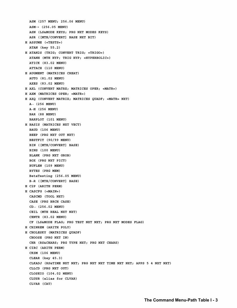
The Command Menu-Path Table I - 3
ASM (257 MENU; 256.06 MENU)
ASM→ (256.05 MENU)
ASN (LS&MODE KEYS; PRG NXT MODES KEYS)
ASR ([MTH/CONVERT] BASE NXT BIT)
H ASSUME («TESTS»)
ATAN (key 55.2)
H ATAN2S (TRIG; CONVERT TRIG; «TRIGO»)
ATANH (MTH HYP; TRIG HYP; «HYPERBOLIC»)
ATICK (83.02 MENU)
ATTACH (110 MENU)
H AUGMENT (MATRICES CREAT)
AUTO (81.02 MENU)
AXES (83.02 MENU)
H AXL (CONVERT MATRX; MATRICES OPER; «MATR»)
H AXM (MATRICES OPER; «MATR»)
H AXQ (CONVERT MATRIX; MATRICES QUADF; «MATR» NXT)
A→ (256 MENU) A→H (256 MENU) BAR (88 MENU)
BARPLOT (101 MENU)
H BASIS (MATRICES NXT VECT)
BAUD (106 MENU)
BEEP (PRG NXT OUT NXT)
BESTFIT (90/99 MENU)
BIN ([MTH/CONVERT] BASE)
BINS (100 MENU)
BLANK (PRG NXT GROB)
BOX (PRG NXT PICT)
BUFLEN (109 MENU)
BYTES (PRG MEM)
BetaTesting (256.05 MENU)
B→R ([MTH/CONVERT] BASE) H C2P (ARITH PERM)
H CASCFG («MAIN»)
CASCMD (TOOL NXT)
CASE (PRG BRCH CASE)
CD→ (256.02 MENU) CEIL (MTH REAL NXT NXT)
CENTR (83.02 MENU)
CF (LS&MODE FLAG; PRG TEST NXT NXT; PRG NXT MODES FLAG)
H CHINREM (ARITH POLY)
H CHOLESKY (MATRICES QUADF)
CHOOSE (PRG NXT IN)
CHR (RS&CHARS; PRG TYPE NXT; PRG NXT CHARS)
H CIRC (ARITH PERM)
CKSM (106 MENU)
CLEAR (key 45.3)
CLKADJ (RS&TIME NXT NXT; PRG NXT NXT TIME NXT NXT; APPS 5 4 NXT NXT)
CLLCD (PRG NXT OUT)
CLOSEIO (104.02 MENU)
CLUSR (alias for CLVAR)
CLVAR (CAT)
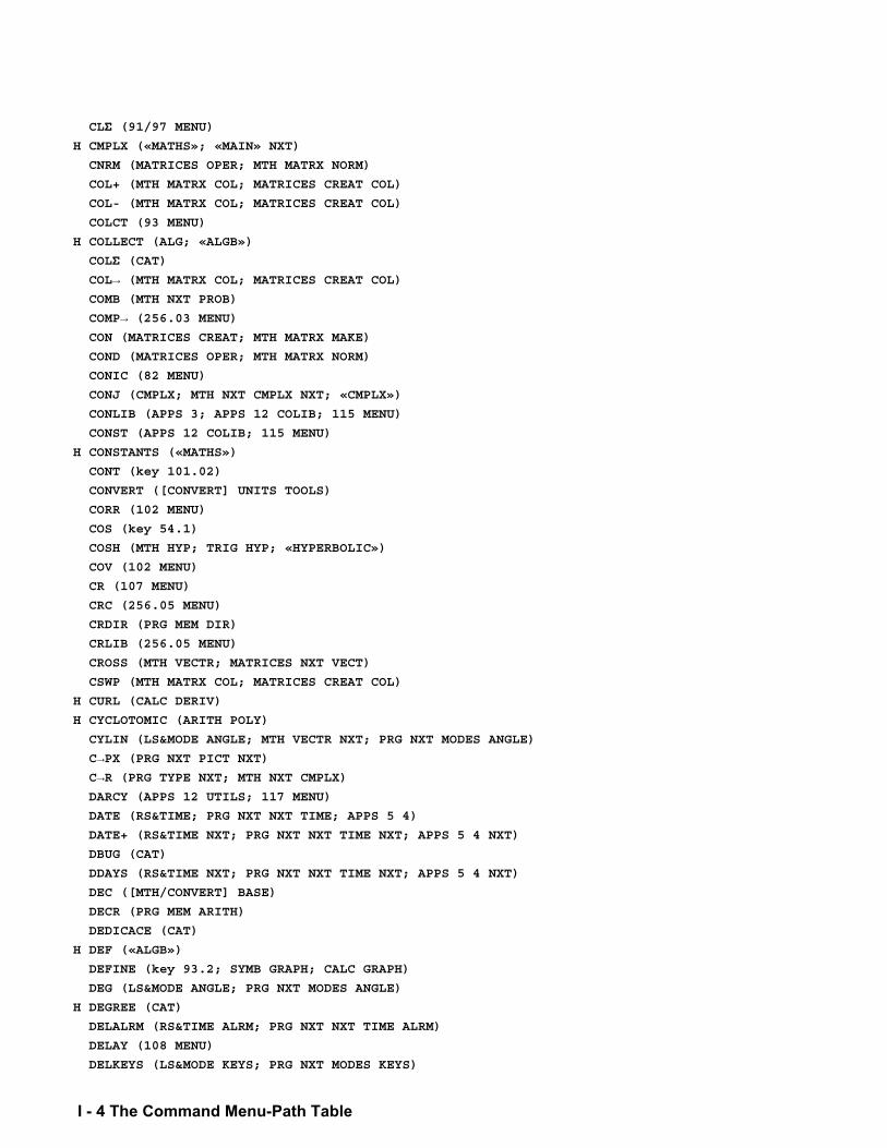
I - 4 The Command Menu-Path Table
CLΣ (91/97 MENU) H CMPLX («MATHS»; «MAIN» NXT)
CNRM (MATRICES OPER; MTH MATRX NORM)
COL+ (MTH MATRX COL; MATRICES CREAT COL)
COL- (MTH MATRX COL; MATRICES CREAT COL)
COLCT (93 MENU)
H COLLECT (ALG; «ALGB»)
COLΣ (CAT) COL→ (MTH MATRX COL; MATRICES CREAT COL) COMB (MTH NXT PROB)
COMP→ (256.03 MENU) CON (MATRICES CREAT; MTH MATRX MAKE)
COND (MATRICES OPER; MTH MATRX NORM)
CONIC (82 MENU)
CONJ (CMPLX; MTH NXT CMPLX NXT; «CMPLX»)
CONLIB (APPS 3; APPS 12 COLIB; 115 MENU)
CONST (APPS 12 COLIB; 115 MENU)
H CONSTANTS («MATHS»)
CONT (key 101.02)
CONVERT ([CONVERT] UNITS TOOLS)
CORR (102 MENU)
COS (key 54.1)
COSH (MTH HYP; TRIG HYP; «HYPERBOLIC»)
COV (102 MENU)
CR (107 MENU)
CRC (256.05 MENU)
CRDIR (PRG MEM DIR)
CRLIB (256.05 MENU)
CROSS (MTH VECTR; MATRICES NXT VECT)
CSWP (MTH MATRX COL; MATRICES CREAT COL)
H CURL (CALC DERIV)
H CYCLOTOMIC (ARITH POLY)
CYLIN (LS&MODE ANGLE; MTH VECTR NXT; PRG NXT MODES ANGLE)
C→PX (PRG NXT PICT NXT) C→R (PRG TYPE NXT; MTH NXT CMPLX) DARCY (APPS 12 UTILS; 117 MENU)
DATE (RS&TIME; PRG NXT NXT TIME; APPS 5 4)
DATE+ (RS&TIME NXT; PRG NXT NXT TIME NXT; APPS 5 4 NXT)
DBUG (CAT)
DDAYS (RS&TIME NXT; PRG NXT NXT TIME NXT; APPS 5 4 NXT)
DEC ([MTH/CONVERT] BASE)
DECR (PRG MEM ARITH)
DEDICACE (CAT)
H DEF («ALGB»)
DEFINE (key 93.2; SYMB GRAPH; CALC GRAPH)
DEG (LS&MODE ANGLE; PRG NXT MODES ANGLE)
H DEGREE (CAT)
DELALRM (RS&TIME ALRM; PRG NXT NXT TIME ALRM)
DELAY (108 MENU)
DELKEYS (LS&MODE KEYS; PRG NXT MODES KEYS)
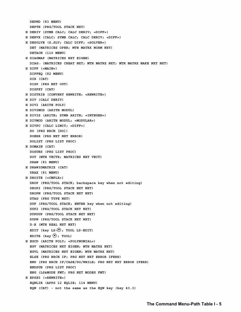
The Command Menu-Path Table I - 5
DEPND (83 MENU)
DEPTH (PRG/TOOL STACK NXT)
H DERIV (SYMB CALC; CALC DERIV; «DIFF»)
H DERVX (CALC; SYMB CALC; CALC DERIV; «DIFF»)
H DESOLVE (S.SLV; CALC DIFF; «SOLVER»)
DET (MATRICES OPER; MTH MATRX NORM NXT)
DETACH (110 MENU)
H DIAGMAP (MATRICES NXT EIGEN)
DIAG→ (MATRICES CREAT NXT; MTH MATRX NXT; MTH MATRX MAKE NXT NXT) H DIFF («MAIN»)
DIFFEQ (82 MENU)
DIR (CAT)
DISP (PRG NXT OUT)
DISPXY (CAT)
H DISTRIB (CONVERT REWRITE; «REWRITE»)
H DIV (CALC DERIV)
H DIV2 (ARITH POLY)
H DIV2MOD (ARITH MODUL)
H DIVIS (ARITH; SYMB ARITH; «INTEGER»)
H DIVMOD (ARITH MODUL; «MODULAR»)
H DIVPC (CALC LIMIT; «DIFF»)
DO (PRG BRCH [DO])
DOERR (PRG NXT NXT ERROR)
DOLIST (PRG LIST PROC)
H DOMAIN (CAT)
DOSUBS (PRG LIST PROC)
DOT (MTH VECTR; MATRICES NXT VECT)
DRAW (81 MENU)
H DRAW3DMATRIX (CAT)
DRAX (81 MENU)
H DROITE («CMPLX»)
DROP (PRG/TOOL STACK; backspace key when not editing)
DROP2 (PRG/TOOL STACK NXT NXT)
DROPN (PRG/TOOL STACK NXT NXT)
DTAG (PRG TYPE NXT)
DUP (PRG/TOOL STACK; ENTER key when not editing)
DUP2 (PRG/TOOL STACK NXT NXT)
DUPDUP (PRG/TOOL STACK NXT NXT)
DUPN (PRG/TOOL STACK NXT NXT)
D→R (MTH REAL NXT NXT) EDIT (key LS-; TOOL LS-EDIT)
EDITB (key ; TOOL)
H EGCD (ARITH POLY; «POLYNOMIAL»)
EGV (MATRICES NXT EIGEN; MTH MATRX NXT)
EGVL (MATRICES NXT EIGEN; MTH MATRX NXT)
ELSE (PRG BRCH IF; PRG NXT NXT ERROR IFERR)
END (PRG BRCH IF/CASE/DO/WHILE; PRG NXT NXT ERROR IFERR)
ENDSUB (PRG LIST PROC)
ENG (LS&MODE FMT; PRG NXT MODES FMT)
H EPSX0 («REWRITE»)
EQNLIB (APPS 12 EQLIB; 114 MENU)
EQW (CAT) - not the same as the EQW key (key 43.3)
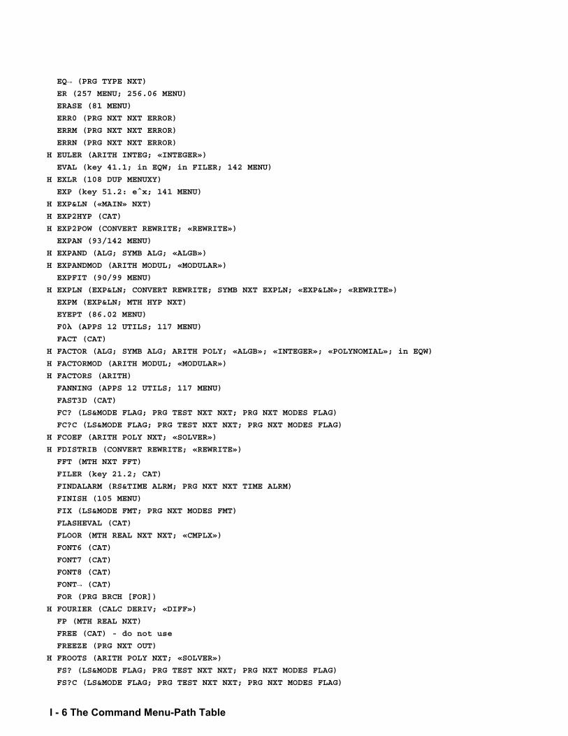
I - 6 The Command Menu-Path Table
EQ→ (PRG TYPE NXT) ER (257 MENU; 256.06 MENU)
ERASE (81 MENU)
ERR0 (PRG NXT NXT ERROR)
ERRM (PRG NXT NXT ERROR)
ERRN (PRG NXT NXT ERROR)
H EULER (ARITH INTEG; «INTEGER»)
EVAL (key 41.1; in EQW; in FILER; 142 MENU)
H EXLR (108 DUP MENUXY)
EXP (key 51.2: e^x; 141 MENU)
H EXP&LN («MAIN» NXT)
H EXP2HYP (CAT)
H EXP2POW (CONVERT REWRITE; «REWRITE»)
EXPAN (93/142 MENU)
H EXPAND (ALG; SYMB ALG; «ALGB»)
H EXPANDMOD (ARITH MODUL; «MODULAR»)
EXPFIT (90/99 MENU)
H EXPLN (EXP&LN; CONVERT REWRITE; SYMB NXT EXPLN; «EXP&LN»; «REWRITE»)
EXPM (EXP&LN; MTH HYP NXT)
EYEPT (86.02 MENU)
F0λ (APPS 12 UTILS; 117 MENU) FACT (CAT)
H FACTOR (ALG; SYMB ALG; ARITH POLY; «ALGB»; «INTEGER»; «POLYNOMIAL»; in EQW)
H FACTORMOD (ARITH MODUL; «MODULAR»)
H FACTORS (ARITH)
FANNING (APPS 12 UTILS; 117 MENU)
FAST3D (CAT)
FC? (LS&MODE FLAG; PRG TEST NXT NXT; PRG NXT MODES FLAG)
FC?C (LS&MODE FLAG; PRG TEST NXT NXT; PRG NXT MODES FLAG)
H FCOEF (ARITH POLY NXT; «SOLVER»)
H FDISTRIB (CONVERT REWRITE; «REWRITE»)
FFT (MTH NXT FFT)
FILER (key 21.2; CAT)
FINDALARM (RS&TIME ALRM; PRG NXT NXT TIME ALRM)
FINISH (105 MENU)
FIX (LS&MODE FMT; PRG NXT MODES FMT)
FLASHEVAL (CAT)
FLOOR (MTH REAL NXT NXT; «CMPLX»)
FONT6 (CAT)
FONT7 (CAT)
FONT8 (CAT)
FONT→ (CAT) FOR (PRG BRCH [FOR])
H FOURIER (CALC DERIV; «DIFF»)
FP (MTH REAL NXT)
FREE (CAT) - do not use
FREEZE (PRG NXT OUT)
H FROOTS (ARITH POLY NXT; «SOLVER»)
FS? (LS&MODE FLAG; PRG TEST NXT NXT; PRG NXT MODES FLAG)
FS?C (LS&MODE FLAG; PRG TEST NXT NXT; PRG NXT MODES FLAG)
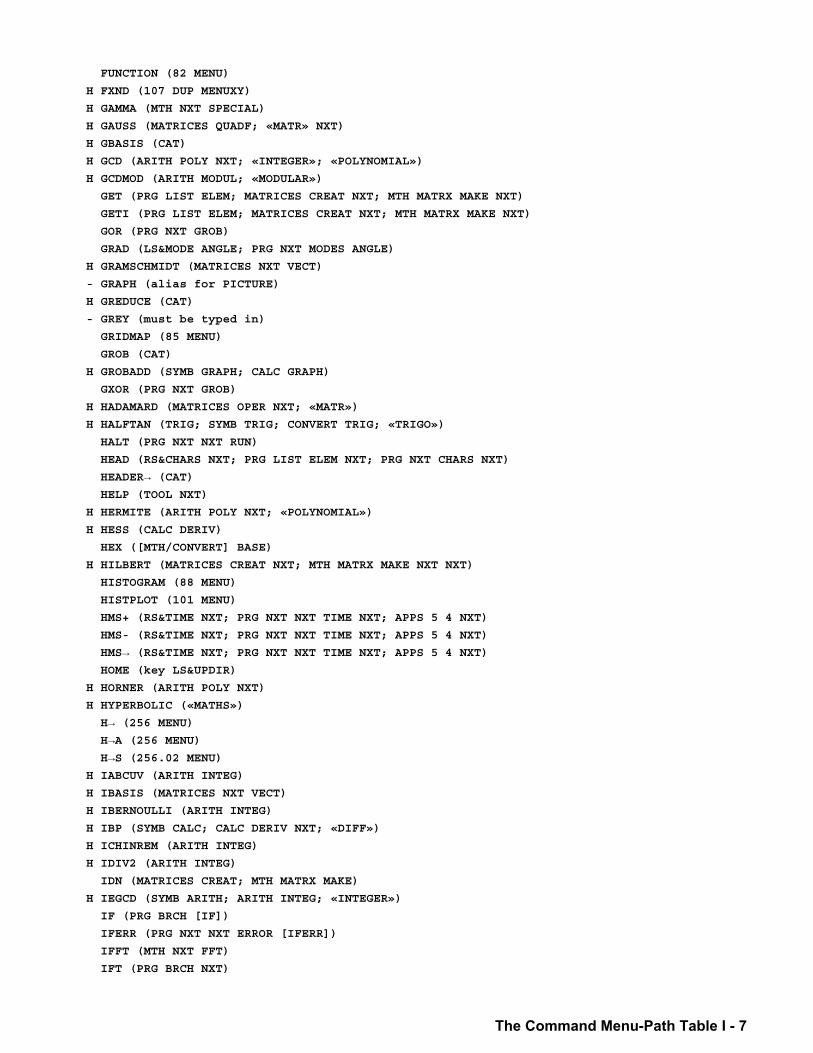
The Command Menu-Path Table I - 7
FUNCTION (82 MENU)
H FXND (107 DUP MENUXY)
H GAMMA (MTH NXT SPECIAL)
H GAUSS (MATRICES QUADF; «MATR» NXT)
H GBASIS (CAT)
H GCD (ARITH POLY NXT; «INTEGER»; «POLYNOMIAL»)
H GCDMOD (ARITH MODUL; «MODULAR»)
GET (PRG LIST ELEM; MATRICES CREAT NXT; MTH MATRX MAKE NXT)
GETI (PRG LIST ELEM; MATRICES CREAT NXT; MTH MATRX MAKE NXT)
GOR (PRG NXT GROB)
GRAD (LS&MODE ANGLE; PRG NXT MODES ANGLE)
H GRAMSCHMIDT (MATRICES NXT VECT)
- GRAPH (alias for PICTURE)
H GREDUCE (CAT)
- GREY (must be typed in)
GRIDMAP (85 MENU)
GROB (CAT)
H GROBADD (SYMB GRAPH; CALC GRAPH)
GXOR (PRG NXT GROB)
H HADAMARD (MATRICES OPER NXT; «MATR»)
H HALFTAN (TRIG; SYMB TRIG; CONVERT TRIG; «TRIGO»)
HALT (PRG NXT NXT RUN)
HEAD (RS&CHARS NXT; PRG LIST ELEM NXT; PRG NXT CHARS NXT)
HEADER→ (CAT) HELP (TOOL NXT)
H HERMITE (ARITH POLY NXT; «POLYNOMIAL»)
H HESS (CALC DERIV)
HEX ([MTH/CONVERT] BASE)
H HILBERT (MATRICES CREAT NXT; MTH MATRX MAKE NXT NXT)
HISTOGRAM (88 MENU)
HISTPLOT (101 MENU)
HMS+ (RS&TIME NXT; PRG NXT NXT TIME NXT; APPS 5 4 NXT)
HMS- (RS&TIME NXT; PRG NXT NXT TIME NXT; APPS 5 4 NXT)
HMS→ (RS&TIME NXT; PRG NXT NXT TIME NXT; APPS 5 4 NXT) HOME (key LS&UPDIR)
H HORNER (ARITH POLY NXT)
H HYPERBOLIC («MATHS»)
H→ (256 MENU) H→A (256 MENU) H→S (256.02 MENU) H IABCUV (ARITH INTEG)
H IBASIS (MATRICES NXT VECT)
H IBERNOULLI (ARITH INTEG)
H IBP (SYMB CALC; CALC DERIV NXT; «DIFF»)
H ICHINREM (ARITH INTEG)
H IDIV2 (ARITH INTEG)
IDN (MATRICES CREAT; MTH MATRX MAKE)
H IEGCD (SYMB ARITH; ARITH INTEG; «INTEGER»)
IF (PRG BRCH [IF])
IFERR (PRG NXT NXT ERROR [IFERR])
IFFT (MTH NXT FFT)
IFT (PRG BRCH NXT)
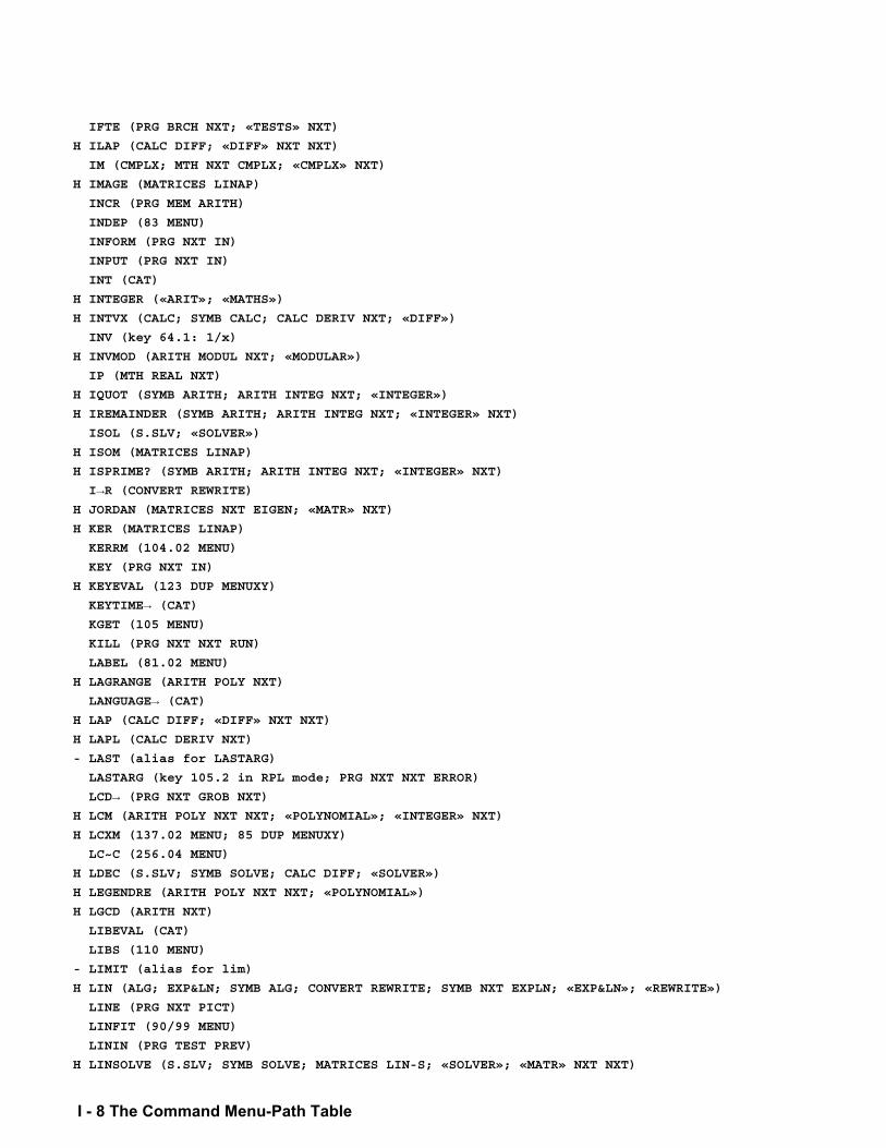
I - 8 The Command Menu-Path Table
IFTE (PRG BRCH NXT; «TESTS» NXT)
H ILAP (CALC DIFF; «DIFF» NXT NXT)
IM (CMPLX; MTH NXT CMPLX; «CMPLX» NXT)
H IMAGE (MATRICES LINAP)
INCR (PRG MEM ARITH)
INDEP (83 MENU)
INFORM (PRG NXT IN)
INPUT (PRG NXT IN)
INT (CAT)
H INTEGER («ARIT»; «MATHS»)
H INTVX (CALC; SYMB CALC; CALC DERIV NXT; «DIFF»)
INV (key 64.1: 1/x)
H INVMOD (ARITH MODUL NXT; «MODULAR»)
IP (MTH REAL NXT)
H IQUOT (SYMB ARITH; ARITH INTEG NXT; «INTEGER»)
H IREMAINDER (SYMB ARITH; ARITH INTEG NXT; «INTEGER» NXT)
ISOL (S.SLV; «SOLVER»)
H ISOM (MATRICES LINAP)
H ISPRIME? (SYMB ARITH; ARITH INTEG NXT; «INTEGER» NXT)
I→R (CONVERT REWRITE) H JORDAN (MATRICES NXT EIGEN; «MATR» NXT)
H KER (MATRICES LINAP)
KERRM (104.02 MENU)
KEY (PRG NXT IN)
H KEYEVAL (123 DUP MENUXY)
KEYTIME→ (CAT) KGET (105 MENU)
KILL (PRG NXT NXT RUN)
LABEL (81.02 MENU)
H LAGRANGE (ARITH POLY NXT)
LANGUAGE→ (CAT) H LAP (CALC DIFF; «DIFF» NXT NXT)
H LAPL (CALC DERIV NXT)
- LAST (alias for LASTARG)
LASTARG (key 105.2 in RPL mode; PRG NXT NXT ERROR)
LCD→ (PRG NXT GROB NXT) H LCM (ARITH POLY NXT NXT; «POLYNOMIAL»; «INTEGER» NXT)
H LCXM (137.02 MENU; 85 DUP MENUXY)
LC~C (256.04 MENU)
H LDEC (S.SLV; SYMB SOLVE; CALC DIFF; «SOLVER»)
H LEGENDRE (ARITH POLY NXT NXT; «POLYNOMIAL»)
H LGCD (ARITH NXT)
LIBEVAL (CAT)
LIBS (110 MENU)
- LIMIT (alias for lim)
H LIN (ALG; EXP&LN; SYMB ALG; CONVERT REWRITE; SYMB NXT EXPLN; «EXP&LN»; «REWRITE»)
LINE (PRG NXT PICT)
LINFIT (90/99 MENU)
LININ (PRG TEST PREV)
H LINSOLVE (S.SLV; SYMB SOLVE; MATRICES LIN-S; «SOLVER»; «MATR» NXT NXT)
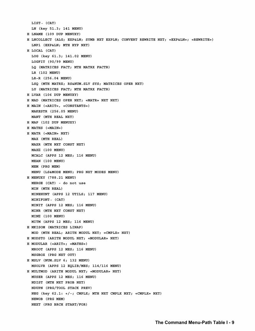
The Command Menu-Path Table I - 9
LIST→ (CAT) LN (key 51.3; 141 MENU)
H LNAME (109 DUP MENUXY)
H LNCOLLECT (ALG; EXP&LN; SYMB NXT EXPLN; CONVERT REWRITE NXT; «EXP&LN»; «REWRITE»)
LNP1 (EXP&LN; MTH HYP NXT)
H LOCAL (CAT)
LOG (key 61.3; 141.02 MENU)
LOGFIT (90/99 MENU)
LQ (MATRICES FACT; MTH MATRX FACTR)
LR (102 MENU)
LR~R (256.04 MENU)
LSQ (MTH MATRX; RS&NUM.SLV SYS; MATRICES OPER NXT)
LU (MATRICES FACT; MTH MATRX FACTR)
H LVAR (106 DUP MENUXY)
H MAD (MATRICES OPER NXT; «MATR» NXT NXT)
H MAIN («ARIT», «CONSTANTS»)
MAKESTR (256.05 MENU)
MANT (MTH REAL NXT)
H MAP (102 DUP MENUXY)
H MATHS («MAIN»)
H MATR («MAIN» NXT)
MAX (MTH REAL)
MAXR (MTH NXT CONST NXT)
MAXΣ (100 MENU) MCALC (APPS 12 MES; 116 MENU)
MEAN (100 MENU)
MEM (PRG MEM)
MENU (LS&MODE MENU; PRG NXT MODES MENU)
H MENUXY (788.21 MENU)
MERGE (CAT) - do not use
MIN (MTH REAL)
MINEHUNT (APPS 12 UTILS; 117 MENU)
MINIFONT→ (CAT) MINIT (APPS 12 MES; 116 MENU)
MINR (MTH NXT CONST NXT)
MINΣ (100 MENU) MITM (APPS 12 MES; 116 MENU)
H MKISOM (MATRICES LINAP)
MOD (MTH REAL; ARITH MODUL NXT; «CMPLX» NXT)
H MODSTO (ARITH MODUL NXT; «MODULAR» NXT)
H MODULAR («ARIT»; «MATHS»)
MROOT (APPS 12 MES; 116 MENU)
MSGBOX (PRG NXT OUT)
H MSLV (NUM.SLV 6; 132 MENU)
MSOLVR (APPS 12 EQLIB/MES; 114/116 MENU)
H MULTMOD (ARITH MODUL NXT; «MODULAR» NXT)
MUSER (APPS 12 MES; 116 MENU)
NDIST (MTH NXT PROB NXT)
NDUPN (PRG/TOOL STACK PREV)
NEG (key 62.1: +/-; CMPLX; MTH NXT CMPLX NXT; «CMPLX» NXT)
NEWOB (PRG MEM)
NEXT (PRG BRCH START/FOR)
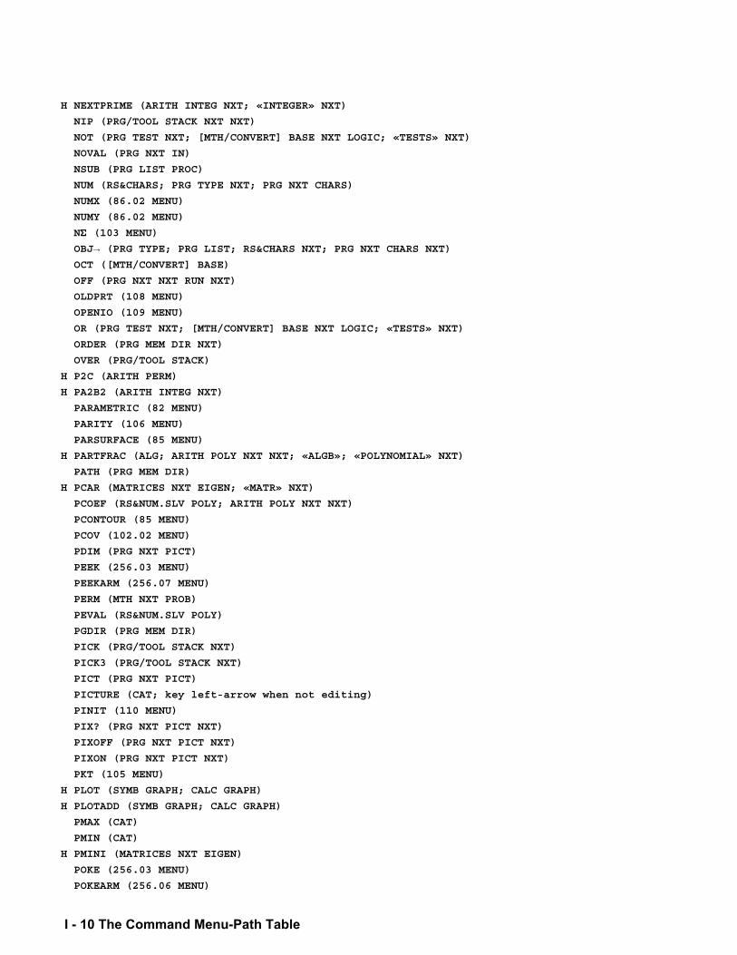
I - 10 The Command Menu-Path Table
H NEXTPRIME (ARITH INTEG NXT; «INTEGER» NXT)
NIP (PRG/TOOL STACK NXT NXT)
NOT (PRG TEST NXT; [MTH/CONVERT] BASE NXT LOGIC; «TESTS» NXT)
NOVAL (PRG NXT IN)
NSUB (PRG LIST PROC)
NUM (RS&CHARS; PRG TYPE NXT; PRG NXT CHARS)
NUMX (86.02 MENU)
NUMY (86.02 MENU)
NΣ (103 MENU) OBJ→ (PRG TYPE; PRG LIST; RS&CHARS NXT; PRG NXT CHARS NXT) OCT ([MTH/CONVERT] BASE)
OFF (PRG NXT NXT RUN NXT)
OLDPRT (108 MENU)
OPENIO (109 MENU)
OR (PRG TEST NXT; [MTH/CONVERT] BASE NXT LOGIC; «TESTS» NXT)
ORDER (PRG MEM DIR NXT)
OVER (PRG/TOOL STACK)
H P2C (ARITH PERM)
H PA2B2 (ARITH INTEG NXT)
PARAMETRIC (82 MENU)
PARITY (106 MENU)
PARSURFACE (85 MENU)
H PARTFRAC (ALG; ARITH POLY NXT NXT; «ALGB»; «POLYNOMIAL» NXT)
PATH (PRG MEM DIR)
H PCAR (MATRICES NXT EIGEN; «MATR» NXT)
PCOEF (RS&NUM.SLV POLY; ARITH POLY NXT NXT)
PCONTOUR (85 MENU)
PCOV (102.02 MENU)
PDIM (PRG NXT PICT)
PEEK (256.03 MENU)
PEEKARM (256.07 MENU)
PERM (MTH NXT PROB)
PEVAL (RS&NUM.SLV POLY)
PGDIR (PRG MEM DIR)
PICK (PRG/TOOL STACK NXT)
PICK3 (PRG/TOOL STACK NXT)
PICT (PRG NXT PICT)
PICTURE (CAT; key left-arrow when not editing)
PINIT (110 MENU)
PIX? (PRG NXT PICT NXT)
PIXOFF (PRG NXT PICT NXT)
PIXON (PRG NXT PICT NXT)
PKT (105 MENU)
H PLOT (SYMB GRAPH; CALC GRAPH)
H PLOTADD (SYMB GRAPH; CALC GRAPH)
PMAX (CAT)
PMIN (CAT)
H PMINI (MATRICES NXT EIGEN)
POKE (256.03 MENU)
POKEARM (256.06 MENU)
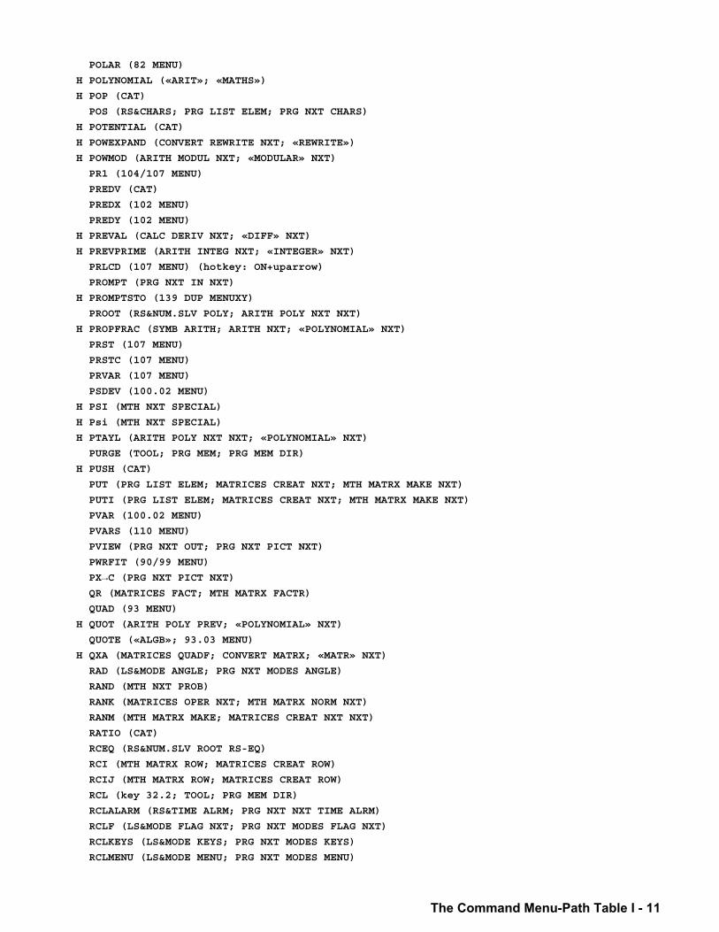
The Command Menu-Path Table I - 11
POLAR (82 MENU)
H POLYNOMIAL («ARIT»; «MATHS»)
H POP (CAT)
POS (RS&CHARS; PRG LIST ELEM; PRG NXT CHARS)
H POTENTIAL (CAT)
H POWEXPAND (CONVERT REWRITE NXT; «REWRITE»)
H POWMOD (ARITH MODUL NXT; «MODULAR» NXT)
PR1 (104/107 MENU)
PREDV (CAT)
PREDX (102 MENU)
PREDY (102 MENU)
H PREVAL (CALC DERIV NXT; «DIFF» NXT)
H PREVPRIME (ARITH INTEG NXT; «INTEGER» NXT)
PRLCD (107 MENU) (hotkey: ON+uparrow)
PROMPT (PRG NXT IN NXT)
H PROMPTSTO (139 DUP MENUXY)
PROOT (RS&NUM.SLV POLY; ARITH POLY NXT NXT)
H PROPFRAC (SYMB ARITH; ARITH NXT; «POLYNOMIAL» NXT)
PRST (107 MENU)
PRSTC (107 MENU)
PRVAR (107 MENU)
PSDEV (100.02 MENU)
H PSI (MTH NXT SPECIAL)
H Psi (MTH NXT SPECIAL)
H PTAYL (ARITH POLY NXT NXT; «POLYNOMIAL» NXT)
PURGE (TOOL; PRG MEM; PRG MEM DIR)
H PUSH (CAT)
PUT (PRG LIST ELEM; MATRICES CREAT NXT; MTH MATRX MAKE NXT)
PUTI (PRG LIST ELEM; MATRICES CREAT NXT; MTH MATRX MAKE NXT)
PVAR (100.02 MENU)
PVARS (110 MENU)
PVIEW (PRG NXT OUT; PRG NXT PICT NXT)
PWRFIT (90/99 MENU)
PX→C (PRG NXT PICT NXT) QR (MATRICES FACT; MTH MATRX FACTR)
QUAD (93 MENU)
H QUOT (ARITH POLY PREV; «POLYNOMIAL» NXT)
QUOTE («ALGB»; 93.03 MENU)
H QXA (MATRICES QUADF; CONVERT MATRX; «MATR» NXT)
RAD (LS&MODE ANGLE; PRG NXT MODES ANGLE)
RAND (MTH NXT PROB)
RANK (MATRICES OPER NXT; MTH MATRX NORM NXT)
RANM (MTH MATRX MAKE; MATRICES CREAT NXT NXT)
RATIO (CAT)
RCEQ (RS&NUM.SLV ROOT RS-EQ)
RCI (MTH MATRX ROW; MATRICES CREAT ROW)
RCIJ (MTH MATRX ROW; MATRICES CREAT ROW)
RCL (key 32.2; TOOL; PRG MEM DIR)
RCLALARM (RS&TIME ALRM; PRG NXT NXT TIME ALRM)
RCLF (LS&MODE FLAG NXT; PRG NXT MODES FLAG NXT)
RCLKEYS (LS&MODE KEYS; PRG NXT MODES KEYS)
RCLMENU (LS&MODE MENU; PRG NXT MODES MENU)
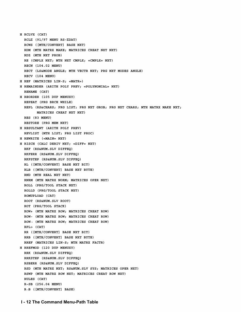
I - 12 The Command Menu-Path Table
H RCLVX (CAT)
RCLΣ (91/97 MENU RS-ΣDAT) RCWS ([MTH/CONVERT] BASE NXT)
RDM (MTH MATRX MAKE; MATRICES CREAT NXT NXT)
RDZ (MTH NXT PROB)
RE (CMPLX NXT; MTH NXT CMPLX; «CMPLX» NXT)
RECN (104.02 MENU)
RECT (LS&MODE ANGLE; MTH VECTR NXT; PRG NXT MODES ANGLE)
RECV (104 MENU)
H REF (MATRICES LIN-S; «MATR»)
H REMAINDER (ARITH POLY PREV; «POLYNOMIAL» NXT)
RENAME (CAT)
H REORDER (105 DUP MENUXY)
REPEAT (PRG BRCH WHILE)
REPL (RS&CHARS; PRG LIST; PRG NXT GROB; PRG NXT CHARS; MTH MATRX MAKE NXT;
MATRICES CREAT NXT NXT)
RES (83 MENU)
RESTORE (PRG MEM NXT)
H RESULTANT (ARITH POLY PREV)
REVLIST (MTH LIST; PRG LIST PROC)
H REWRITE («MAIN» NXT)
H RISCH (CALC DERIV NXT; «DIFF» NXT)
RKF (RS&NUM.SLV DIFFEQ)
RKFERR (RS&NUM.SLV DIFFEQ)
RKFSTEP (RS&NUM.SLV DIFFEQ)
RL ([MTH/CONVERT] BASE NXT BIT)
RLB ([MTH/CONVERT] BASE NXT BYTE)
RND (MTH REAL NXT NXT)
RNRM (MTH MATRX NORM; MATRICES OPER NXT)
ROLL (PRG/TOOL STACK NXT)
ROLLD (PRG/TOOL STACK NXT)
ROMUPLOAD (CAT)
ROOT (RS&NUM.SLV ROOT)
ROT (PRG/TOOL STACK)
ROW+ (MTH MATRX ROW; MATRICES CREAT ROW)
ROW- (MTH MATRX ROW; MATRICES CREAT ROW)
ROW→ (MTH MATRX ROW; MATRICES CREAT ROW) RPL> (CAT)
RR ([MTH/CONVERT] BASE NXT BIT)
RRB ([MTH/CONVERT] BASE NXT BYTE)
RREF (MATRICES LIN-S; MTH MATRX FACTR)
H RREFMOD (120 DUP MENUXY)
RRK (RS&NUM.SLV DIFFEQ)
RRKSTEP (RS&NUM.SLV DIFFEQ)
RSBERR (RS&NUM.SLV DIFFEQ)
RSD (MTH MATRX NXT; RS&NUM.SLV SYS; MATRICES OPER NXT)
RSWP (MTH MATRX ROW NXT; MATRICES CREAT ROW NXT)
RULES (CAT)
R~SB (256.04 MENU)
R→B ([MTH/CONVERT] BASE)
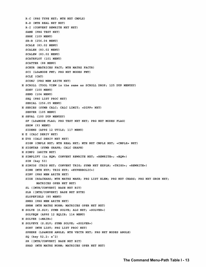
The Command Menu-Path Table I - 13
R→C (PRG TYPE NXT; MTH NXT CMPLX) R→D (MTH REAL NXT NXT) R→I (CONVERT REWRITE NXT NXT) SAME (PRG TEST NXT)
SBRK (109 MENU)
SB~B (256.04 MENU)
SCALE (83.02 MENU)
SCALEH (83.02 MENU)
SCALEW (83.02 MENU)
SCATRPLOT (101 MENU)
SCATTER (88 MENU)
SCHUR (MATRICES FACT; MTH MATRX FACTR)
SCI (LS&MODE FMT; PRG NXT MODES FMT)
SCLΣ (CAT) SCONJ (PRG MEM ARITH NXT)
H SCROLL (TOOL VIEW is the same as SCROLL DROP; 125 DUP MENUXY)
SDEV (100 MENU)
SEND (104 MENU)
SEQ (PRG LIST PROC NXT)
SERIAL (256.05 MENU)
H SERIES (SYMB CALC; CALC LIMIT; «DIFF» NXT)
SERVER (105 MENU)
H SEVAL (100 DUP MENUXY)
SF (LS&MODE FLAG; PRG TEST NXT NXT; PRG NXT MODES FLAG)
SHOW (93 MENU)
SIDENS (APPS 12 UTILS; 117 MENU)
H Σ (CALC DERIV NXT) H ΣVX (CALC DERIV NXT NXT) SIGN (CMPLX NXT; MTH REAL NXT; MTH NXT CMPLX NXT; «CMPLX» NXT)
H SIGNTAB (SYMB GRAPH; CALC GRAPH)
H SIMP2 (ARITH NXT)
H SIMPLIFY (in EQW; CONVERT REWRITE NXT; «REWRITE»; «EQW»)
SIN (key 53)
H SINCOS (TRIG NXT; CONVERT TRIG; SYMB NXT EXPLN; «TRIGO»; «REWRITE»)
SINH (MTH HYP; TRIG HYP; «HYPERBOLIC»)
SINV (PRG MEM ARITH NXT)
SIZE (RS&CHARS; MTH MATRX MAKE; PRG LIST ELEM; PRG NXT CHARS; PRG NXT GROB NXT;
MATRICES OPER NXT NXT)
SL ([MTH/CONVERT] BASE NXT BIT)
SLB ([MTH/CONVERT] BASE NXT BYTE)
SLOPEFIELD (85 MENU)
SNEG (PRG MEM ARITH NXT)
SNRM (MTH MATRX NORM; MATRICES OPER NXT NXT)
H SOLVE (S.SLV; SYMB SOLVE; ALG NXT; «SOLVER»)
SOLVEQN (APPS 12 EQLIB; 114 MENU)
H SOLVER («MAIN»)
H SOLVEVX (S.SLV; SYMB SOLVE; «SOLVER»)
SORT (MTH LIST; PRG LIST PROC NXT)
SPHERE (LS&MODE ANGLE; MTH VECTR NXT; PRG NXT MODES ANGLE)
SQ (key 52.2: x^2)
SR ([MTH/CONVERT] BASE NXT BIT)
SRAD (MTH MATRX NORM; MATRICES OPER NXT NXT)
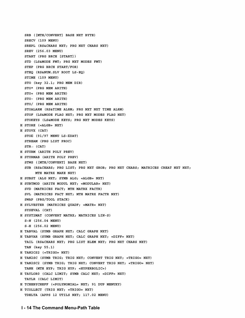
I - 14 The Command Menu-Path Table
SRB ([MTH/CONVERT] BASE NXT BYTE)
SRECV (109 MENU)
SREPL (RS&CHARS NXT; PRG NXT CHARS NXT)
SREV (256.03 MENU)
START (PRG BRCH [START])
STD (LS&MODE FMT; PRG NXT MODES FMT)
STEP (PRG BRCH START/FOR)
STEQ (RS&NUM.SLV ROOT LS-EQ)
STIME (109 MENU)
STO (key 32.1; PRG MEM DIR)
STO* (PRG MEM ARITH)
STO+ (PRG MEM ARITH)
STO- (PRG MEM ARITH)
STO/ (PRG MEM ARITH)
STOALARM (RS&TIME ALRM; PRG NXT NXT TIME ALRM)
STOF (LS&MODE FLAG NXT; PRG NXT MODES FLAG NXT)
STOKEYS (LS&MODE KEYS; PRG NXT MODES KEYS)
H STORE («ALGB» NXT)
H STOVX (CAT)
STOΣ (91/97 MENU LS-ΣDAT) STREAM (PRG LIST PROC)
STR→ (CAT) H STURM (ARITH POLY PREV)
H STURMAB (ARITH POLY PREV)
STWS ([MTH/CONVERT] BASE NXT)
SUB (RS&CHARS; PRG LIST; PRG NXT GROB; PRG NXT CHARS; MATRICES CREAT NXT NXT;
MTH MATRX MAKE NXT)
H SUBST (ALG NXT; SYMB ALG; «ALGB» NXT)
H SUBTMOD (ARITH MODUL NXT; «MODULAR» NXT)
SVD (MATRICES FACT; MTH MATRX FACTR)
SVL (MATRICES FACT NXT; MTH MATRX FACTR NXT)
SWAP (PRG/TOOL STACK)
H SYLVESTER (MATRICES QUADF; «MATR» NXT)
SYSEVAL (CAT)
H SYST2MAT (CONVERT MATRX; MATRICES LIN-S)
S~N (256.04 MENU)
S→H (256.02 MENU) H TABVAL (SYMB GRAPH NXT; CALC GRAPH NXT)
H TABVAR (SYMB GRAPH NXT; CALC GRAPH NXT; «DIFF» NXT)
TAIL (RS&CHARS NXT; PRG LIST ELEM NXT; PRG NXT CHARS NXT)
TAN (key 55.1)
H TAN2CS2 («TRIGO» NXT)
H TAN2SC (SYMB TRIG; TRIG NXT; CONVERT TRIG NXT; «TRIGO» NXT)
H TAN2SC2 (SYMB TRIG; TRIG NXT; CONVERT TRIG NXT; «TRIGO» NXT)
TANH (MTH HYP; TRIG HYP; «HYPERBOLIC»)
H TAYLOR0 (CALC LIMIT; SYMB CALC NXT; «DIFF» NXT)
TAYLR (CALC LIMIT)
H TCHEBYCHEFF («POLYNOMIAL» NXT; 91 DUP MENUXY)
H TCOLLECT (TRIG NXT; «TRIGO» NXT)
TDELTA (APPS 12 UTILS NXT; 117.02 MENU)
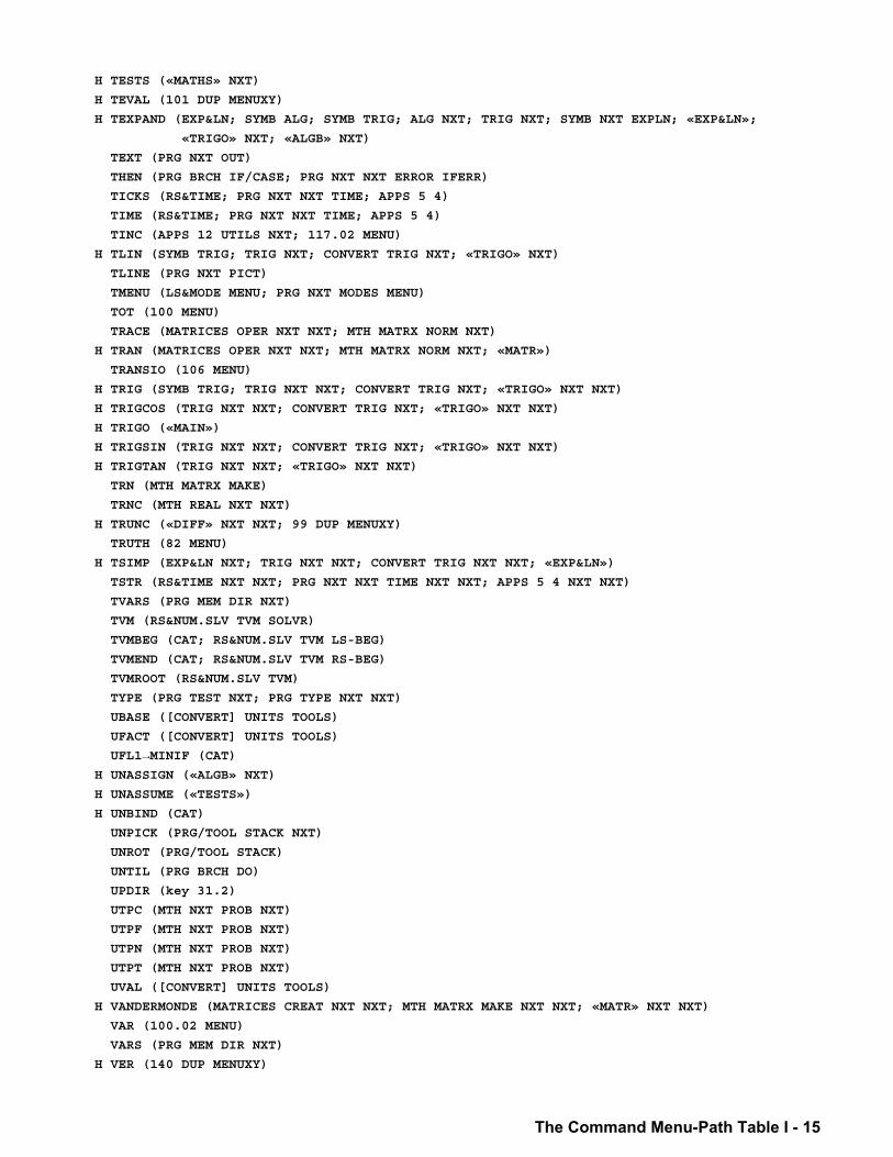
The Command Menu-Path Table I - 15
H TESTS («MATHS» NXT)
H TEVAL (101 DUP MENUXY)
H TEXPAND (EXP&LN; SYMB ALG; SYMB TRIG; ALG NXT; TRIG NXT; SYMB NXT EXPLN; «EXP&LN»;
«TRIGO» NXT; «ALGB» NXT)
TEXT (PRG NXT OUT)
THEN (PRG BRCH IF/CASE; PRG NXT NXT ERROR IFERR)
TICKS (RS&TIME; PRG NXT NXT TIME; APPS 5 4)
TIME (RS&TIME; PRG NXT NXT TIME; APPS 5 4)
TINC (APPS 12 UTILS NXT; 117.02 MENU)
H TLIN (SYMB TRIG; TRIG NXT; CONVERT TRIG NXT; «TRIGO» NXT)
TLINE (PRG NXT PICT)
TMENU (LS&MODE MENU; PRG NXT MODES MENU)
TOT (100 MENU)
TRACE (MATRICES OPER NXT NXT; MTH MATRX NORM NXT)
H TRAN (MATRICES OPER NXT NXT; MTH MATRX NORM NXT; «MATR»)
TRANSIO (106 MENU)
H TRIG (SYMB TRIG; TRIG NXT NXT; CONVERT TRIG NXT; «TRIGO» NXT NXT)
H TRIGCOS (TRIG NXT NXT; CONVERT TRIG NXT; «TRIGO» NXT NXT)
H TRIGO («MAIN»)
H TRIGSIN (TRIG NXT NXT; CONVERT TRIG NXT; «TRIGO» NXT NXT)
H TRIGTAN (TRIG NXT NXT; «TRIGO» NXT NXT)
TRN (MTH MATRX MAKE)
TRNC (MTH REAL NXT NXT)
H TRUNC («DIFF» NXT NXT; 99 DUP MENUXY)
TRUTH (82 MENU)
H TSIMP (EXP&LN NXT; TRIG NXT NXT; CONVERT TRIG NXT NXT; «EXP&LN»)
TSTR (RS&TIME NXT NXT; PRG NXT NXT TIME NXT NXT; APPS 5 4 NXT NXT)
TVARS (PRG MEM DIR NXT)
TVM (RS&NUM.SLV TVM SOLVR)
TVMBEG (CAT; RS&NUM.SLV TVM LS-BEG)
TVMEND (CAT; RS&NUM.SLV TVM RS-BEG)
TVMROOT (RS&NUM.SLV TVM)
TYPE (PRG TEST NXT; PRG TYPE NXT NXT)
UBASE ([CONVERT] UNITS TOOLS)
UFACT ([CONVERT] UNITS TOOLS)
UFL1→MINIF (CAT) H UNASSIGN («ALGB» NXT)
H UNASSUME («TESTS»)
H UNBIND (CAT)
UNPICK (PRG/TOOL STACK NXT)
UNROT (PRG/TOOL STACK)
UNTIL (PRG BRCH DO)
UPDIR (key 31.2)
UTPC (MTH NXT PROB NXT)
UTPF (MTH NXT PROB NXT)
UTPN (MTH NXT PROB NXT)
UTPT (MTH NXT PROB NXT)
UVAL ([CONVERT] UNITS TOOLS)
H VANDERMONDE (MATRICES CREAT NXT NXT; MTH MATRX MAKE NXT NXT; «MATR» NXT NXT)
VAR (100.02 MENU)
VARS (PRG MEM DIR NXT)
H VER (140 DUP MENUXY)
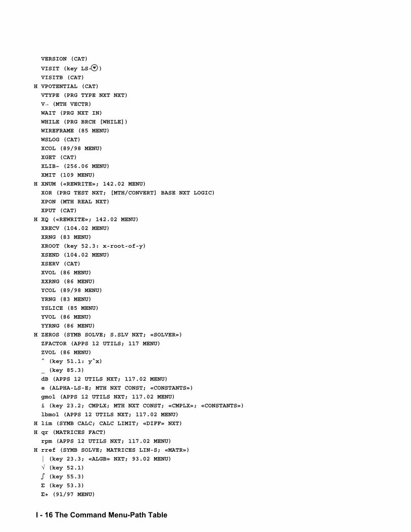
I - 16 The Command Menu-Path Table
VERSION (CAT)
VISIT (key LS-)
VISITB (CAT)
H VPOTENTIAL (CAT)
VTYPE (PRG TYPE NXT NXT)
V→ (MTH VECTR) WAIT (PRG NXT IN)
WHILE (PRG BRCH [WHILE])
WIREFRAME (85 MENU)
WSLOG (CAT)
XCOL (89/98 MENU)
XGET (CAT)
XLIB~ (256.06 MENU)
XMIT (109 MENU)
H XNUM («REWRITE»; 142.02 MENU)
XOR (PRG TEST NXT; [MTH/CONVERT] BASE NXT LOGIC)
XPON (MTH REAL NXT)
XPUT (CAT)
H XQ («REWRITE»; 142.02 MENU)
XRECV (104.02 MENU)
XRNG (83 MENU)
XROOT (key 52.3: x-root-of-y)
XSEND (104.02 MENU)
XSERV (CAT)
XVOL (86 MENU)
XXRNG (86 MENU)
YCOL (89/98 MENU)
YRNG (83 MENU)
YSLICE (85 MENU)
YVOL (86 MENU)
YYRNG (86 MENU)
H ZEROS (SYMB SOLVE; S.SLV NXT; «SOLVER»)
ZFACTOR (APPS 12 UTILS; 117 MENU)
ZVOL (86 MENU)
^ (key 51.1: y^x)
_ (key 85.3)
dB (APPS 12 UTILS NXT; 117.02 MENU)
e (ALPHA-LS-E; MTH NXT CONST; «CONSTANTS»)
gmol (APPS 12 UTILS NXT; 117.02 MENU)
i (key 23.2; CMPLX; MTH NXT CONST; «CMPLX»; «CONSTANTS»)
lbmol (APPS 12 UTILS NXT; 117.02 MENU)
H lim (SYMB CALC; CALC LIMIT; «DIFF» NXT)
H qr (MATRICES FACT)
rpm (APPS 12 UTILS NXT; 117.02 MENU)
H rref (SYMB SOLVE; MATRICES LIN-S; «MATR»)
| (key 23.3; «ALGB» NXT; 93.02 MENU)
√ (key 52.1) ∫ (key 55.3) Σ (key 53.3) Σ+ (91/97 MENU)
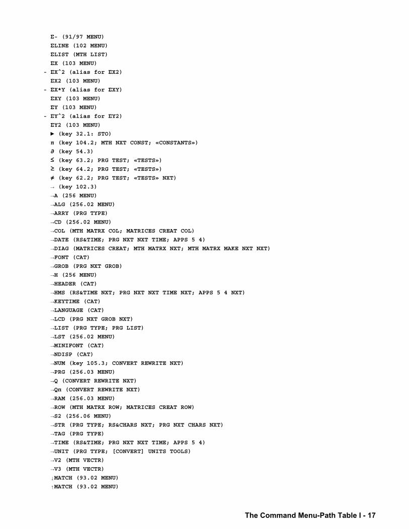
The Command Menu-Path Table I - 17
Σ- (91/97 MENU) ΣLINE (102 MENU) ΣLIST (MTH LIST) ΣX (103 MENU) - ΣX^2 (alias for ΣX2) ΣX2 (103 MENU) - ΣX*Y (alias for ΣXY) ΣXY (103 MENU) ΣY (103 MENU) - ΣY^2 (alias for ΣY2) ΣY2 (103 MENU) (key 32.1: STO) π (key 104.2; MTH NXT CONST; «CONSTANTS») ∂ (key 54.3) ≤ (key 63.2; PRG TEST; «TESTS») ≥ (key 64.2; PRG TEST; «TESTS») ≠ (key 62.2; PRG TEST; «TESTS» NXT) → (key 102.3) →A (256 MENU) →ALG (256.02 MENU) →ARRY (PRG TYPE) →CD (256.02 MENU) →COL (MTH MATRX COL; MATRICES CREAT COL) →DATE (RS&TIME; PRG NXT NXT TIME; APPS 5 4) →DIAG (MATRICES CREAT; MTH MATRX NXT; MTH MATRX MAKE NXT NXT) →FONT (CAT) →GROB (PRG NXT GROB) →H (256 MENU) →HEADER (CAT) →HMS (RS&TIME NXT; PRG NXT NXT TIME NXT; APPS 5 4 NXT) →KEYTIME (CAT) →LANGUAGE (CAT) →LCD (PRG NXT GROB NXT) →LIST (PRG TYPE; PRG LIST) →LST (256.02 MENU) →MINIFONT (CAT) →NDISP (CAT) →NUM (key 105.3; CONVERT REWRITE NXT) →PRG (256.03 MENU) →Q (CONVERT REWRITE NXT) →Qп (CONVERT REWRITE NXT) →RAM (256.03 MENU) →ROW (MTH MATRX ROW; MATRICES CREAT ROW) →S2 (256.06 MENU) →STR (PRG TYPE; RS&CHARS NXT; PRG NXT CHARS NXT) →TAG (PRG TYPE) →TIME (RS&TIME; PRG NXT NXT TIME; APPS 5 4) →UNIT (PRG TYPE; [CONVERT] UNITS TOOLS) →V2 (MTH VECTR) →V3 (MTH VECTR) ↓MATCH (93.02 MENU) ↑MATCH (93.02 MENU)

I - 18 The Command Menu-Path Table
∆LIST (MTH LIST) ΠLIST (MTH LIST) H ∞ (key 102.2; «CONSTANTS») « (key 95.3)
» (key 95.3)
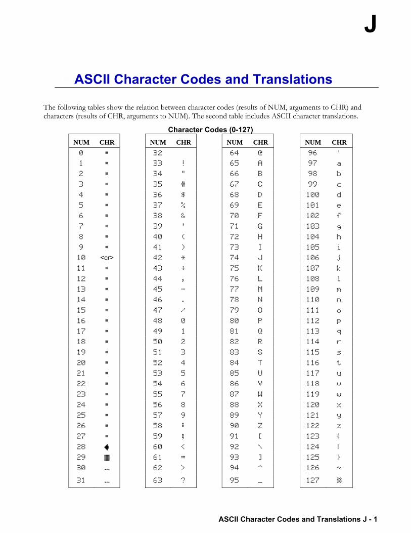
J
ASCII Character Codes and Translations J - 1
16.ASCII Character Codes and Translations
The following tables show the relation between character codes (results of NUM, arguments to CHR) and characters (results of CHR, arguments to NUM). The second table includes ASCII character translations.
Character Codes (0-127) NUM CHR NUM CHR NUM CHR NUM CHR 0 32 64 @ 96 '
1 33 ! 65 A 97 a
2 34 " 66 B 98 b
3 35 # 67 C 99 c
4 36 $ 68 D 100 d
5 37 % 69 E 101 e
6 38 & 70 F 102 f
7 39 ' 71 G 103 g
8 40 ( 72 H 104 h
9 41 ) 73 I 105 i
10 <cr> 42 * 74 J 106 j
11 43 + 75 K 107 k
12 44 , 76 L 108 l
13 45 - 77 M 109 m
14 46 . 78 N 110 n
15 47 / 79 O 111 o
16 48 0 80 P 112 p
17 49 1 81 Q 113 q
18 50 2 82 R 114 r
19 51 3 83 S 115 s
20 52 4 84 T 116 t
21 53 5 85 U 117 u
22 54 6 86 V 118 v
23 55 7 87 W 119 w
24 56 8 88 X 120 x
25 57 9 89 Y 121 y
26 58 : 90 Z 122 z
27 59 ; 91 [ 123
28 60 < 92 \ 124 |
29 | 61 = 93 ] 125
30 ... 62 > 94 ^ 126 ~
31 ... 63 ? 95 _ 127
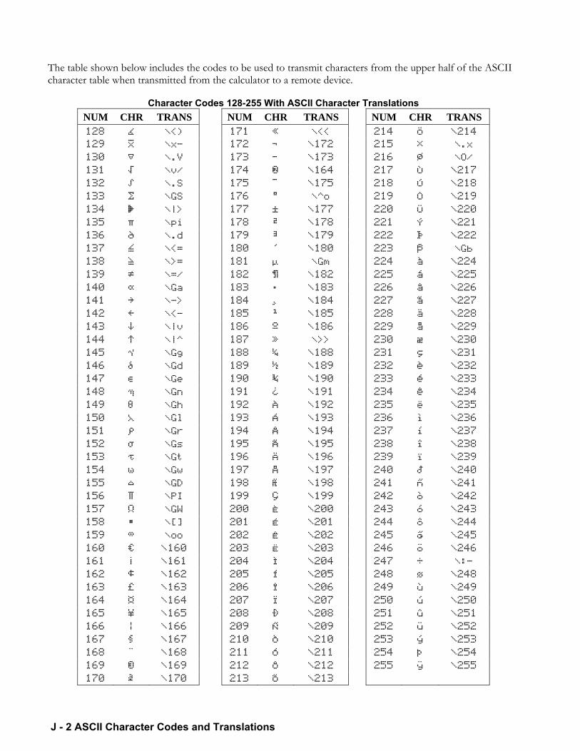
J - 2 ASCII Character Codes and Translations
The table shown below includes the codes to be used to transmit characters from the upper half of the ASCII character table when transmitted from the calculator to a remote device.
Character Codes 128-255 With ASCII Character Translations
NUM CHR TRANS NUM CHR TRANS NUM CHR TRANS 128 \<) 171 « \<< 214 Ö \214
129 \x- 172 ¬ \172 215 × \.x 130 ‚ \.V 173 − \173 216 Ø \O/ 131 ƒ \v/ 174 ® \164 217 Ù \217
132 „ \.S 175 ¯ \175 218 Ú \218
133 … \GS 176 ° \^o 219 Û \219
134 † \|> 177 ± \177 220 Ü \220
135 ‡ \pi 178 ² \178 221 Ý \221
136 ˆ \.d 179 ³ \179 222 Þ \222
137 ‰ \<= 180 ´ \180 223 ß \Gb 138 Š \>= 181 µ \Gm 224 à \224
139 ‹ \=/ 182 ¶ \182 225 á \225
140 Œ \Ga 183 · \183 226 â \226
141 \-> 184 ¸ \184 227 ã \227
142 \<- 185 ¹ \185 228 ä \228
143 \|v 186 º \186 229 å \229
144 \|^ 187 » \>> 230 æ \230
145 ‘ \Gg 188 ¼ \188 231 ç \231
146 ’ \Gd 189 ½ \189 232 è \232
147 “ \Ge 190 ¾ \190 233 é \233
148 ” \Gn 191 ¿ \191 234 ê \234
149 • \Gh 192 À \192 235 ë \235
150 – \Gl 193 Á \193 236 ì \236
151 — \Gr 194 Â \194 237 í \237
152 ˜ \Gs 195 Ã \195 238 î \238
153 ™ \Gt 196 Ä \196 239 ï \239
154 š \Gw 197 Å \197 240 ð \240
155 › \GD 198 Æ \198 241 ñ \241
156 œ \PI 199 Ç \199 242 ò \242
157 \GW 200 È \200 243 ó \243
158 \[] 201 É \201 244 ô \244
159 Ÿ \oo 202 Ê \202 245 õ \245
160 \160 203 Ë \203 246 ö \246
161 ¡ \161 204 Ì \204 247 ÷ \:- 162 ¢ \162 205 Í \205 248 ø \248
163 £ \163 206 Î \206 249 ù \249
164 ¤ \164 207 Ï \207 250 ú \250
165 ¥ \165 208 Ð \208 251 û \251
166 ¦ \166 209 Ñ \209 252 ü \252
167 § \167 210 Ò \210 253 ý \253
168 ¨ \168 211 Ó \211 254 þ \254
169 © \169 212 Ô \212 255 ÿ \255
170 ª \170 213 Õ \213
Index - 1
17.Index Symbols
(Subtract) 3-222 ! (Factorial) 3-214 % (Percent) 3-214 %CH 3-26 %T 3-179 %TILE (Percentile of a list) 2-10 * (Multiply) 3-219 / (Divide) 3-223 ? (Undefined) 3-212, 4-81 ^ (Power) 3-209 _ (Unit attachment) 3-215 | (Where) 3-209 MATCH 3-101 ↓MATCH 3-100 + (Add) 3-220 < (Less than) 3-215 = (Equal) 3-223 == (Logical Equality) 3-224 > (Greater than) 3-217 % (Store) 3-225 « » (Program delimeters) 3-215 √ (Square Root) 3-210 ∫ (Integrate) 3-211 ≤ (Less than or Equal) 3-216 → (Create Local) 3-225 →A 6-2 →ALG 6-5 →ARRY 3-12 →CD 6-3 →COL 3-30 →DATE 3-39 →DIAG 3-45 →FONT 3-67 →GROB 3-74 →H 6-3 →HEADER 3-76 →HMS 3-79 →KEYTIME 3-89 →LANGUAGE 3-91 →LCD 3-92 →LIST 3-94 →LST 6-6 →MINIFONT 3-105 →NDISP 3-108 →NUM 3-111 →PRG 6-6 →Q 3-135 →Qπ 3-135
→MAP 6-2 →ROW 3-152 →S2 6-4 →STR 3-176 →TAG 3-180 →TIME 3-183 →UNIT 3-191 →V2 3-195 →V3 3-195 ∂ (Derivative) 3-213 ≠ (Not equal) 3-219 1D Elastic Collisions (4, 5) 5-24 ≥ (Greater than or Equal) 3-218 ∞ (Infinity) 3-212, 4-81
A A→ 6-2 A→H 6-2 ABCUV 3-4, 4-12 ABS 3-4 ACK 3-4 ACKALL 3-4 ACOS 3-5 ACOS2S 3-6, 4-12 ACOSH 3-6 ADD 3-7 ADDTMOD 3-8, 4-12 ADDTOREAL 3-8, 4-13 ALGB 3-8, 4-13 ALOG 3-8 ALRMDAT D-2 AMORT 3-8 AND 3-8 Angular Mechanics (4, 2) 5-23 Angular Motion (8, 4) 5-36 ANIMATE 3-9 Animating a Graphical Image 2-39
Animation of Successive Taylor's Polynomials 2-30 ANS 3-10 APEEK 6-1 APPLY 3-10 Applying a Program to an Array 2-20 ARC 3-10 ARCHIVE 3-11 ARG 3-11 ARIT 3-12, 4-13 ARM→ 6-35 ARRY→ 3-12 ASCII Character Codes and Translations J-1
2 - Index
ASIN 3-12 ASIN2C 3-14, 4-14 ASIN2T 3-14, 4-14 ASINH 3-14 ASM 6-8 ASM→ 6-34 ASN 3-14 ASR 3-15 ASSUME 3-16, 4-14 ATAN 3-16 ATAN2S 3-17, 4-15 ATANH 3-17 ATICK 3-18 ATTACH 3-18 AUGMENT 3-19, 4-15 AUTO 3-19 AXES 3-20 AXL 3-20, 4-15 AXM 3-20, 4-16 AXQ 3-20, 4-16
B B→R 3-24 BAR 3-20 BARPLOT 3-21 BASIS 3-22, 4-16 BAUD 3-22 BDISP (Binary Display) 2-7 BEEP 3-22 Beeping to Get Attention 1-45 Bernoulli Equation (3, 2) 5-19 Bessel Functions 2-29 BESTFIT 3-22 BIN 3-22 BINS 3-23 Bipolar Transistors (13, 3) 5-53 Black Body Radiation (6, 6) 5-31 BLANK 3-23 BOX 3-23 Brewster's Law (9, 3) 5-38 BUFLEN 3-24 BYTES 3-24
C C→PX 3-38 C→R 3-39 C2P 3-24, 4-17 Calculations in a Program 1-2 Cantilever Deflection (1, 7) 5-7 Cantilever Moment (1, 9) 5-8 Cantilever Shear (1, 10) 5-8 Cantilever Slope (1, 8) 5-7 Capacitive Energy (2, 9) 5-13 Capacitor Charge (2, 13) 5-14 CAS Commands Introduction 4-1 CAS directory, CASDIR, The 4-2
CAS Operations 4-1 CAS Settings 4-2 CAS Settings, Selecting 4-2 CAS, Using the 4-4 CASCFG 3-25, 4-17 CASCMD 3-25, 4-17 CASE 3-25 Causing and Analyzing Errors 1-32 CD→ 6-3 CEIL 3-25 CENTR 3-26 Centripetal Force (4, 3) 5-23 CF 3-26 CHINREM 3-27, 4-17 CHOLESKY 3-27, 4-18 CHOOSE 3-27 CHR 3-27 CIRC 3-28, 4-18 Circle (11, 1) 5-44 Circular Motion (8, 5) 5-36 Circular Ring (11, 5) 5-46 CKSM 3-28 CLEAR 3-28 CLKADJ 3-28 CLLCD 3-29 CLOSEIO 3-29 CLVAR 3-29 CLΣ 3-29 CMPLX 3-29 CNRM 3-30 COL 3-30 COL+ 3-31 COL→ 3-30 COLCT 3-31 COLLECT 3-31, 4-19 Columns and Beams (1) 5-3 COLΣ 3-31 COMB 3-32 COMP→ 6-5 Command Menu-Path Table, The I-1 Compatibility with Other Calculators 4-4 Compiled Local Variables 1-10 Computer Algebra Commands 4-1 CON 3-32 COND 3-33 Conditional Structures and Commands, Using 1-13 Conduction (6, 3) 5-29 Conduction + Convection (6, 5) 5-30 Cone (12, 1) 5-47 CONIC 3-33 Conical Pendulum (10, 3) 5-42 CONJ 3-34 CONLIB 3-34
Index - 3
CONST 3-35 CONSTANTS 3-35, 4-19 CONT 3-35 Contents of a Program, The 1-1 Contents of the Reserved Variables D-2 Convection (6, 4) 5-30 CONVERT 3-35 Converting Between Number Bases 2-22 Converting Procedures from Algebraic to RPN 2-27 CORR 3-35 COS 3-36 COSH 3-36 Coulomb's Law (2, 1) 5-10 COV 3-37 CR 3-37 CRC 6-4 CRDIR 3-37 Creating Local Variables 1-7 Creating Programs on a Computer 1-7 Creating User-Defined Functions as Programs 1-10 Critical Angle (9, 2) 5-38 CRLIB 6-6 CROSS 3-37 CST D-3 CSWP 3-38 CURL 3-38, 4-19 Current Divider (2, 4) 5-11 CYCLOTOMIC 3-38, 4-20 CYLIN 3-38 Cylinder (12, 2) 5-48 Cylindrical Capacitor (2,19) 5-16
D D→R 3-54 DARCY 3-39 Data Input Commands 1-35 Data Output Commands 1-47 DATE 3-39 DATE+ 3-40 DBUG 3-40 DC Capacitor Current (2, 12) 5-14 DC Inductor Voltage (2, 14) 5-14 DDAYS 3-40
Dealing with unexpected CAS results or messages 4-4 DEC 3-41 DECR 3-41 DEDICACE 3-41, 4-20 DEF 3-41, 4-20 DEFINE 3-41 Defining the Scope of Local Variables 1-9 Definite Loop Structures, Using 1-17 DEG 3-42
DEGREE 3-42, 4-21 DELALARM 3-42 DELAY 3-42 DELKEYS 3-42 DEPND 3-43 DEPTH 3-44 DERIV 3-44, 4-21 DERVX 3-44, 4-21 DESOLVE 3-44, 4-22 DET 3-44 DETACH 3-44 Development Library, The 6-1 DIAG→ 3-45 DIAGMAP 3-45, 4-22 DIFF 3-45, 4-23 DIFFEQ 3-46 DIR 3-47 Disassemblers 6-34 DISP 3-47 DISP FREEZE HALT CONT for Input, Using 1-37 Displaying a Binary Integer 2-5 DISPXY 3-47 DISTRIB 3-48, 4-23 DIV 3-48, 4-23 DIV2 3-48, 4-23 DIV2MOD 3-48, 4-24 DIVIS 3-48, 4-24 DIVMOD 3-48, 4-25 DIVPC 3-48, 4-25 DLIST 3-95 dn 3-48, 4-26 DO 3-48 DOERR 3-49 DOLIST 3-49 DOMAIN 3-50, 4-25 DOSUBS 3-50 DOT 3-50 Drag Force (4, 6) 5-24 DRAW 3-51 DRAW3DMATRIX 3-51 DRAX 3-51 DROITE 3-52, 4-26 DROP 3-52 DROP2 3-52 DROPN 3-52 DTAG 3-52 DUP 3-53 DUP2 3-53 DUPDUP 3-53 DUPN 3-53
E e 3-54 Eccentric Columns (1, 2) 5-4
4 - Index
EDIT 3-54 EDITB 3-55 EGCD 3-55, 4-27 EGV 3-55 EGVL 3-55 Elastic Buckling (1, 1) 5-4 Electricity (2) 5-9 Ellipse (11, 2) 5-44 ELSE 3-55 END 3-56 ENDSUB 3-56 ENG 3-56 Entering and Executing Programs 1-3 Entry Point Library: Extable, The 6-35 ENVSTACK D-4 EPSX0 3-56, 4-27 EQ D-4 EQ→ 3-57 EQNLIB 3-56 Equation Reference 5-1 EQW 3-57 ERASE 3-57 ERR0 3-57 ERRM 3-57 ERRN 3-58 Error and Status Messages A-1 Escape Velocity (8, 7) 5-36 EULER 3-58, 4-28 EVAL 3-58 Evaluating Local Names 1-8 EX&LN 3-59 Examples and Help 4-4 EXCO (Expand and Collect Completely) 2-15 EXITED D-4 EXLR 3-59, 4-28 EXP 3-59 EXP&LN 4-28 EXP2HYP 3-60, 4-28 EXP2POW 3-60, 4-29 EXPAN 3-60 EXPAND 3-60, 4-29 Expanding and Collecting Completely 2-14 EXPANDMOD 3-60, 4-30 EXPFIT 3-60 EXPLN 3-60, 4-30 EXPM 3-60 EXPR D-4 Extending the CAS 4-4 EYEPT 3-61
F F0λ 3-61 FACT 3-61 FACTOR 3-62, 4-30 FACTORMOD 3-62, 4-31
FACTORS 3-62, 4-31 FANNING 3-62 FAST3D 3-62 FC? 3-63 FC?C 3-63 FCOEF 3-63, 4-31 FDISTRIB 3-64, 4-32 FFT 3-64 FIB1 (Fibonacci Numbers, Recursive Version) 2-1 FIB2 (Fibonacci Numbers, Loop Version) 2-2 Fibonacci Numbers 2-1 FIBT (Comparing Program-Execution Time) 2-3 FILER 3-64 FINDALARM 3-64 FINISH 3-65 FIX 3-65 Flags, Using 1-25 FLASHEVAL 3-65 FLOOR 3-66 Flow in Full Pipes (3, 4) 5-21 Flow with Losses (3, 3) 5-20 Fluids (3) 5-18 FONT→ 3-67 FONT6 3-66 FONT7 3-66 FONT8 3-66 FOR 3-67 Force between Wires (7, 2) 5-32 Forces and Energy (4) 5-21 FOURIER 3-68, 4-32 FP 3-68 FREE 3-68 FREEZE 3-68 FROOTS 3-69, 4-33 FS? 3-69 FS?C 3-69 Full Command and Function Reference 3-1 FUNCTION 3-70 FXND 3-71, 4-33
G GAMMA 3-71 Gases (5) 5-25 GAUSS 3-71, 4-33 GBASIS 3-71, 4-34 GCD 3-71, 4-34 GCDMOD 3-71, 4-35 GET 3-71 GETADR 6-36 GETI 3-72 GETNAME 6-35 GETNAMES 6-36 GOR 3-73
Index - 5
GRAD 3-73 GRAMSCHMIDT 3-73, 4-35 GREDUCE 3-73, 4-35 GRIDMAP 3-73 GROB 3-74 GROBADD 3-74 GXOR 3-75
H H→ 6-3 H→A 6-2 H→S 6-3 HADAMARD 3-75, 4-36 HALFTAN 3-75, 4-36 HALT 3-75 HEAD 3-75 HEADER→ 3-76 Heat Capacity (6, 1) 5-29 Heat Transfer (6) 5-28 HELP 3-76, 4-36 HERMITE 3-76, 4-37 HESS 3-76, 4-37 HEX 3-76 HILBERT 3-77, 4-37 HISTOGRAM 3-77 HISTPLOT 3-77 HMS 3-78 HMS+ 3-78 HMS→ 3-79 HOME 3-79 Hooke's Law (4, 4) 5-23 HORNER 3-79, 4-38
I i 3-80 I→R 3-88 IABCUV 3-80, 4-38 IBASIS 3-80, 4-38 IBERNOULLI 3-80, 4-39 IBP 3-80, 4-39 ICHINREM 3-80, 4-40 Ideal Gas Law (5, 1) 5-25 Ideal Gas State Change (5, 2) 5-26 IDIV2 3-81, 4-40 IDN 3-80 IEGCD 3-81, 4-40 IF 3-81 IFERR 3-81 IFFT 3-82 IFT 3-83 IFTE 3-83 ILAP 3-83, 4-41 IM 3-83 IMAGE 3-84, 4-41 INCR 3-84 Indefinite Loop Structures, Using 1-21
INDEP 3-84 Inductive Energy (2, 10) 5-13 INFORM 3-85 INFORM and CHOOSE for Input, Using 1-42 Input 1-35 INPUT 3-86 INPUT ENTER for Input, Using 1-38 INT 3-86, 4-41 INTEGER 3-87, 4-42 INTVX 3-87, 4-42 INV 3-87 Inverse-Function Solver 2-38 INVMOD 3-87, 4-42 IOPAR D-4 IP 3-87 IQUOT 3-87, 4-43 IREMAINDER 3-87, 4-43 Isentropic Flow (5, 5) 5-26 ISOL 3-87 ISOM 3-88, 4-43 Isothermal Expansion (5, 3) 5-26 ISPRIME? 3-88, 4-44
J JFETs (13, 4) 5-53 JORDAN 3-88, 4-44
K KER 3-88, 4-45 KERRM 3-88 KEY 3-89 KEY for Keystroke Input, Using 1-46 Keyboard Shortcuts G-1 KEYEVAL 3-89 KEYTIME→ 3-89 KGET 3-90 KILL 3-90 Kinetic Theory (5, 8) 5-28
L LABEL 3-90 Labeling and Displaying Output as Strings 1-48 Labeling Output with Tags 1-47 LAGRANGE 3-90, 4-45 LANGUAGE→ 3-91 LAP 3-91, 4-45 LAPL 3-91, 4-46 LAST 3-91 LASTARG 3-91 Law of Gravitation (4, 7) 5-24 Law of Refraction (9, 1) 5-37 LC~C 6-5 LCD→ 3-92 LCM 3-92, 4-46 LCXM 3-92, 4-46 LDEC 3-92, 4-47
6 - Index
LEGENDRE 3-92, 4-47 LGCD 3-92, 4-48 LIBEVAL 3-92 LIBS 3-93 lim 3-93, 4-48 LIMIT 3-93, 4-48 LIN 3-93, 4-48 LINE 3-93 Linear Mechanics (4, 1) 5-22 Linear Motion (8, 1) 5-35 LINFIT 3-94 LININ 3-94 LINSOLVE 3-94, 4-49 LIST→ 3-94 LN 3-95 LNAME 3-96, 4-49 LNCOLLECT 3-97, 4-49 LNP1 3-97 LOCAL 3-97, 4-50 Local Variables, Using 1-7 LOG 3-97 LOGFIT 3-98 Longitudinal Waves (15, 2) 5-58 Loop Counters, Using 1-24 Loop Structures, Using 1-17 LQ 3-98 LR 3-98 LR~R 6-5 LSQ 3-99 LU 3-99 LVAR 3-100, 4-50
M MAD 3-100, 4-51 Magnetic (B) Field in Solenoid (7, 3) 5-33 Magnetic (B) Field in Toroid (7, 4) 5-33 Magnetism (7) 5-31 MAIN 3-100, 4-51 MAKESTR 6-4 Making an Error Trap 1-33 MANT 3-100 MAP 3-100 MASD.INI D-6 Mass-Energy Relation (4, 8) 5-24 Mass-Spring System (10, 1) 5-41 MATHS 3-101, 4-51 MATR 3-101, 4-52 MAX 3-101 MAXR 3-102 MAXS 3-102 MCALC 3-102 MEAN 3-103 MEDIAN (Median of Statistics Data) 2-11 Median of Statistics Data 2-10 MEM 3-103
MENU 3-103 Menu-Number Table, The H-1 Menus for Input, Using 1-50 Menus to Run Programs, Using 1-50 Menus with Programs, Using 1-49 MENUXY 3-104, 4-52 MERGE 3-104 MHpar D-6 MIN 3-104 MINEHUNT 3-104 MINIFONT→ 3-105 Minimum and Maximum Array Elements 2-16 MINIT 3-105 MINR 3-106 MINS 3-106 MITM 3-106 MKISOM 3-106, 4-53
MNX (Minimum or Maximum ElementVersion 1) 2-16
MNX2 (Minimum or Maximum Element- Version 2) 2-18 MOD 3-106 MODSTO 3-107, 4-53 MODULAR 3-107, 4-53 Mohr's Circle (14, 4) 5-57 Motion (8) 5-34 Mpar D-6 MROOT 3-107 MSGBOX 3-107 MSGBOX to Display Output, Using 1-49 MSLV 3-107, 4-54 MSOLVR 3-107 MULTI (Multiple Execution) 2-14 MULTMOD 3-108, 4-54 MUSER 3-108
N n1, n2, D-6 NAMES (Check List for Exactly Two Names) 2-24 NDIST 3-108 NDUPN 3-109 NEG 3-109 NEWOB 3-109 NEXT 3-110 NEXTPRIME 3-110, 4-55 NIP 3-110 Nmines D-6 NMOS Transistors (13, 2) 5-52 nop 6-35 Normal Stress (14, 1) 5-55 NOT 3-110 NOVAL 3-111 NS 3-111 NSUB 3-111
Index - 7
NUM 3-112 NUMX 3-112 NUMY 3-112
O OBJ→ 3-113 Object in Free Fall (8, 2) 5-35 Object Sizes E-1 OCT 3-113 OFF 3-113 Ohm's Law and Power (2, 2) 5-10 OLDPRT 3-114 OPENIO 3-114 Optics (9) 5-37 OR 3-114 ORDER 3-115 Oscillations (10) 5-40 Output 1-46 OVER 3-115
P π (Pi) 3-213 P2C 3-115, 4-55 PA2B2 3-115, 4-55 PAD (Pad with Leading Spaces) 2-5 Parallel Processing with Lists F-1 Parallelepiped (12, 3) 5-48 PARAMETRIC 3-116 PARITY 3-116 PARSURFACE 3-117 PARTFRAC 3-118, 4-56 PATH 3-118 Pausing to Display Output 1-48 PCAR 3-118, 4-56 PCOEF 3-118 PCONTOUR 3-118 PCOV 3-119 PDIM 3-119 PEEK 6-1 PEEKARM 6-2 PERM 3-120 PEVAL 3-120 PGDIR 3-120 PICK 3-121 PICK3 3-121 PICT 3-121 PICTURE 3-121 PINIT 3-122 PIX? 3-122 PIXOFF 3-122 PIXON 3-122 PKT 3-122 Plane Geometry (11) 5-43 Plate Capacitor (2, 18) 5-16 PLIST 3-95 PLOT 3-123
PLOTADD 3-123 PMAX 3-123 PMIN 3-123 PMINI 3-124, 4-56 PN Step Junctions (13, 1) 5-51 Points to note when choosing settings 4-3 POKE 6-1 POKEARM 6-2 POLAR 3-124 POLYNOMIAL 3-125, 4-57 Polytropic Processes (5, 4) 5-26 POP 3-125 POS 3-125 POTENTIAL 3-125, 4-57 POWEXPAND 3-125, 4-57 POWMOD 3-125, 4-58 PPAR D-6 PR1 3-125 PREDV 3-126 PREDX 3-126 PREDY 3-127 PRESERVE (Save and Restore Previous Status) 2-6 Pressure at Depth (3, 1) 5-19 PREVAL 3-127, 4-58 PREVPRIME 3-127, 4-58 PRLCD 3-128 Programmatic Use of Statistics and Plotting 2-34 Projectile Motion (8, 3) 5-35 PROMPT 3-128 PROMPT CONT for Input, Using 1-35 PROMPTSTO 3-128 PROOT 3-128 PROPFRAC 3-129, 4-59 PRST 3-129 PRSTC 3-129 PRTPAR D-8 PRVAR 3-129 PSDEV 3-130 PSI 3-130 Psi 3-130 PTAYL 3-130, 4-59 PURGE 3-131 PUSH 3-131 PUT 3-131 PUTI 3-132 PVAR 3-133 PVARS 3-133 PVIEW 3-134 PWRFIT 3-134 PX→C 3-134
Q qr 3-135
8 - Index
QR 3-136 QUAD 3-136 QUOT 3-136, 4-59 QUOTE 3-136 QXA 3-137, 4-60
R R~SB 6-5 R→B 3-156 R→C 3-156 R→D 3-157 R→I 3-157 RAD 3-137 RAND 3-137 RANK 3-137 RANM 3-138 RATIO 3-138 RC Transient (2, 15) 5-15 RCEQ 3-139 RCI 3-139 RCIJ 3-139 RCL 3-139 RCLALARM 3-140 RCLF 3-140 RCLKEYS 3-141 RCLMENU 3-141 RCLS 3-141 RCLVX 3-141, 4-60 RCWS 3-142 RDM 3-142 RDZ 3-142 RE 3-143 Real Gas Law (5, 6) 5-27 Real Gas State Change (5, 7) 5-27 REALASSUME D-8 Recalling and Storing the Flag States 1-27 RECN 3-143 RECT 3-143 Rectangle (11, 3) 5-45 RECV 3-144 REF 3-144, 4-60 References 5-59 Regular Polygon (11, 4) 5-45 REMAINDER 3-144, 4-61 RENAME 3-144 REORDER 3-144, 4-61 REPEAT 3-144 REPL 3-144 RES 3-145 Reserved Variables D-1 Resonant Frequency (2, 17) 5-16 RESTORE 3-146 RESULTANT 3-146, 4-61 REVLIST 3-146 REWRITE 3-147, 4-62
RISCH 3-147, 4-62 RKF 3-147 RKFERR 3-147 RKFSTEP 3-148 RL 3-148 RL Transient (2, 16) 5-15 RLB 3-148 RLC Current Delay (2, 11) 5-14 RND 3-149 RNRM 3-149 ROLL 3-150 ROLLD 3-150 ROMUPLOAD 3-150 ROOT 3-150 ROT 3-151 ROW 3-151 ROW+ 3-151 ROW→ 3-151 RPL Programming 1-1 RPL Programming Examples 2-1 RPL> 3-152 RR 3-152 RRB 3-153 rref 3-153, 4-63 RREF 3-153, 4-62 RREFMOD 3-153, 4-63 RRK 3-153 RRKSTEP 3-154 RSBERR 3-155 RSD 3-155 RSWP 3-156 RULES 3-156
S S~N 6-4 S→H 6-3 s1, s2, D-9 SAME 3-157 SB~B 6-5 SBRK 3-157 SCALE 3-158 SCALEH 3-158 SCALEW 3-158 SCATRPLOT 3-158 SCATTER 3-159 SCHUR 3-159 SCI 3-160 SCLS 3-160 SCONJ 3-160 SCROLL 3-160 SDEV 3-161 SEND 3-161 SEQ 3-161 SERIAL 6-4 SERIES 3-162, 4-64
Index - 9
Series and Parallel C (2, 7) 5-12 Series and Parallel L (2, 8) 5-13 Series and Parallel R (2, 6) 5-12 SERVER 3-162 Setting, Clearing, and Testing Flags 1-26 SETTS (Superimposing Taylor's polynomials) 2-32 SEVAL 3-162, 4-64 SF 3-162 Shear Stress (14, 2) 5-56 SHOW 3-162 SIDENS 3-163 SIGMA 3-163, 4-65 SIGMAVX 3-163, 4-65 SIGN 3-163 SIGNTAB 3-164, 4-65 SIMP2 3-164, 4-66 Simple Deflection (1, 3) 5-5 Simple Harmonic (10, 5) 5-42 Simple Moment (1, 5) 5-6 Simple Pendulum (10, 2) 5-41 Simple Shear (1, 6) 5-6 Simple Slope (1, 4) 5-5 SIMPLIFY 3-164, 4-66 SIN 3-164 SINCOS 3-164, 4-67 Single-Stepping through a Program 1-29 SINH 3-164 SINTP (Converting a Plot to a Graphics Object) 2-31 Sinusoidal Current (2, 23) 5-18 Sinusoidal Voltage (2, 22) 5-18 SINV 3-165 SIZE 3-165 SL 3-165 SLB 3-166 SLINE 3-93 SLIST 3-95 SLOPEFIELD 3-166 SNEG 3-167 SNRM 3-167 Solenoid Inductance (2, 20) 5-17 Solid Geometry (12) 5-47 Solid State Devices (13) 5-49 SOLVE 3-167, 4-67 SOLVEQN 3-167 SOLVER 3-168 SOLVEVX 3-168, 4-68 SORT 3-168 Sound Waves (15, 3) 5-58 Source References E-5 SPHERE 3-168 Sphere (12, 4) 5-49 Spherical Reflection (9, 4) 5-39
Spherical Refraction (9, 5) 5-39 SQ 3-168 SR 3-169 SRAD 3-169 SRB 3-169 SRECV 3-169 SREPL 3-170 SREV 6-3 START 3-170 STARTED D-8 STARTEQW D-9 STARTERR D-9 STARTOFF D-9 STARTRECV D-9 STARTSEND D-9 STARTUP D-9 STD 3-171 STEP 3-172 STEQ 3-172 STIME 3-172 STO 3-172 STO 3-174 STO* 3-175 STO/ 3-175 STO+ 3-174 STOALARM 3-173 STOF 3-173 STOKEYS 3-174 Stopping a Program for Keystroke Input 1-46 STORE 3-174, 4-68 STOS 3-176 STOVX 3-174, 4-68 STR→ 3-176 Straight Wire (7, 1) 5-32 STREAM 3-176 Stress Analysis (14) 5-54 Stress on an Element (14, 3) 5-56 STURM 3-177, 4-69 STURMAB 3-177, 4-69 STWS 3-177 SUB 3-177 Subroutines, Using 1-28 SUBST 3-178, 4-69 SUBTMOD 3-178, 4-70 Summations Instead of Loops, Using 1-25 SVD 3-178 SVL 3-178 SWAP 3-179 SX 3-200 SX2 3-200 SXY 3-205 SY 3-206 SY2 3-206 SYLVESTER 3-179, 4-70
10 - Index
Symbolic Integration Patterns E-2 SYSEVAL 3-179 SYST2MAT 3-179, 4-71 System Flags C-1
T Table of Units B-1 TABVAL 3-180, 4-71 TABVAR 3-180, 4-71 TAIL 3-180 TAN 3-180 TAN2CS2 3-181, 4-72 TAN2SC 3-181, 4-72 TAN2SC2 3-181, 4-73 TANH 3-181 TAYLOR0 3-181, 4-73 TAYLR 3-181 TCHEBYCHEFF 3-182, 4-73 TCOLLECT 3-182, 4-74 TDELTA 3-182 Technical Reference E-1 Techniques used in SINTP 2-31 Terminal Velocity (8, 6) 5-36 Testing Conditions 1-11 TESTS 3-182, 4-74 Tests and Conditional Structures, Using 1-11 TEVAL 3-182 TEXPAND 3-183, 4-74 TEXT 3-183 THEN 3-183 Thermal Expansion (6, 2) 5-29 Thin Lens (9, 6) 5-39 TICKS 3-183 TIME 3-183 TINC 3-184 TLIN 3-184, 4-74 TLINE 3-184 TMENU 3-184 TOFF D-9 Tools of the development library, The 6-1 Toroid Inductance (2, 21) 5-17 Torsional Pendulum (10, 4) 5-42 TOT 3-185 TRACE 3-185 Trace Mode 2-37 TRAN 3-185 TRANSIO 3-185 Transverse Waves (15,1) 5-58 Trapping Errors 1-32 Triangle (11, 6) 5-46 TRIG 3-186, 4-75 TRIGCOS 3-186, 4-75 TRIGO 3-186, 4-76 Trigonometric Expansions E-4 TRIGSIN 3-186, 4-76
TRIGTAN 3-186, 4-76 TRN 3-186 TRNC 3-186 TRUNC 3-187, 4-77 TRUTH 3-187 TSA (Animating Taylor's Polynomials) 2-33 TSIMP 3-188, 4-77 TSTR 3-188 Turning Off the hp49g+/hp48gII from a Program 1-52 TVARS 3-188 TVM 3-188 TVMBEG 3-189 TVMEND 3-189 TVMROOT 3-189 TYPE 3-189 Types of Flags 1-26
U UBASE 3-190 UFACT 3-190 UFL1→MINIF 3-191 UNASSIGN 3-191, 4-77 UNASSUME 3-191, 4-78 UNBIND 3-191, 4-78 Understanding Programming 1-1 UNPICK 3-191 UNROT 3-191 UNTIL 3-192 UPDIR 3-192 UTPC 3-192 UTPF 3-192 UTPN 3-193 UTPT 3-193 UVAL 3-194
V V→ 3-194 VANDERMONDE 3-195, 4-78 VAR 3-196 VARS 3-196 VER 3-196, 4-79 Verifying Program Arguments 2-24 VERSION 3-196 Viewing and Editing Programs 1-6 VISIT 3-196 VISITB 3-197 Voltage Divider (2, 3) 5-11 VPAR D-9 VPOTENTIAL 3-197, 4-79 VTYPE 3-197
W WAIT 3-197 WAIT for Keystroke Input, Using 1-46 Waves (15) 5-57 WHILE 3-198
Index - 11
Wire Resistance (2, 5) 5-11 WIREFRAME 3-198 WSLOG 3-199
X XCOL 3-201 XGET 3-201 XLIB~ 6-4 XMIT 3-201 XNUM 3-202, 4-79 XOR 3-202 XPON 3-202 XPUT 3-203 XQ 3-203, 4-80 XRECV 3-203 XRNG 3-203 XROOT 3-204 XSEND 3-204 XSERV 3-205 XVOL 3-205 XXRNG 3-205
Y
YCOL 3-206 YRNG 3-206 YSLICE 3-207 YVOL 3-207 YYRNG 3-208
Z ZEROS 3-208, 4-80 ZFACTOR 3-208 ZPAR D-10 ZVOL 3-208
Greek Letters αENTER D-2 βENTER D-3 Σ (Sigma Minus) 3-213 Σ (Summation) 3-212 Σ+ (Sigma Plus) 3-212 ΣDAT D-10 ΣPAR D-11