How is it made?

Global Positioning System (GPS)

Joseph Khoury

June 14, 2011

Abstract

Recently, after a family trip, a friend of mine decided to go back to use his old paper map in his trav-

els and to put his GPS receiver to rest for ever. This came after a series of deceptions by this little device

with the annoying automated voice and the 4" screen and the constantly lost signal, his words not mine.

The latest of these deceptions was a trip from Ottawa to Niagara Falls which took a turn in the US. Ad-

mittedly, such a turn is normal especially if the GPS is programmed to take the shortest distance, except

that my friend’s family did not have passports on them that day.

Let us face it, if you have a GPS, you must have experienced some set backs here and there. But the

times when the trip went smoothly without any wrong turn, you must have deep down appreciated the

magic and ingenuity that transforms a little device into a holding hand that takes you from point A to

point B , sometimes thousands of kilometers apart. It is indeed a "scary" thing to have someone watch-

ing your every move from somewhere "very high".

Next time you plan a trip, read this note before and use your time on the road to try to reveal to your

co-travelers (with as little mathematics as possible) the magic behind this technology. It works every

time I want to put my kids to sleep on a long trip.

1 A bit of History

The idea of locating one’s position on the surface of the planet goes back deep in human history. Ancient

civilizations like the Greek, Persian and Arab were able to develop navigational tools (like the Astrolabe)

to locate the position of ships in high seas. But let us not go that deep in History, after all we are talking

about a very recent technology.

The following are the main highlights in the history of the Global Positioning System:

• The story started n 1957 when the Soviet Union launched its satellite named Sputnik. Just days

1

after the launching of Sputnik, two American scientists were able track its orbit simply by recording

changes in the satellite radio frequency.

• In the 1960s, the American Navy designed a navigation system for its submarines fleet consisting of

10 satellites. At that time, the signal reception was very slow taking up to several hours to pick up a

satellite signal. Great efforts were made to improve signal reception.

• In the early 1970s, engineers Ivan Getting and Bradford Parkinson led a Defense Department project

to provide continuous navigation information, leading to the development of GPS (formally known

as NAVSTAR GPS) in 1973.

• Year 1978 marked the launching of the first GPS satellite by the US military.

• In 1980, the military activates atomic clocks onboard of GPS satellites.

• Year 1983 was a turning point in the development of the GPS system to a new one that we use today,

but it came with a very high cost. Soviet fighters jets shot down a civilian airplane of the Korean

Airline (Flight 007) after it had gone lost over Soviet territory, killing all 269 on board.. The tragedy

prompted US President Ronald Reagan to declassify the GPS project and cleared the way to allow

the civilian use of the GPS system.

• After many setbacks and delays over a decade, full operational capability with 24 GPS satellites in

orbit was announced in 1995.

• In 2000, Selective Availability is phased out four years after the executive order issued by U.S. Pres-

ident Bill Clinton. Compared to the 100 meters accuracy previously allowed, civilians could now

achieve 10 – 15 meters accuracy. This created a boom in the GPS devices production industry.

• In 2005, the GPS constellation consisted of 32 satellites, out of which 24 are operational and 8 are

ready to take over in case of others fail.

• Continuous efforts are always underway to launch new and improved satellites for both military

and civilian uses.

2 The GPS constellation

As explained above, the GPS system is a constellation of satellites out of which 24 are operational at all

times and others operate as backups in case of failures. These satellites are distributed in six inclined

orbital planes making an angle of 55 degree with the plane of the horizontal plane of the equator and

each orbit contains (at least) four operational satellites. Each satellite orbits the Earth almost twice every

24 hours at an altitude of approximately 20,200 km above the surface of the planet. As you can imagine,

there are many reasons for choosing the tilting angle of the orbital planes, the altitude of the satellites,

2

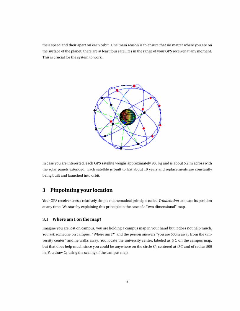
their speed and their apart on each orbit. One main reason is to ensure that no matter where you are on

the surface of the planet, there are at least four satellites in the range of your GPS receiver at any moment.

This is crucial for the system to work.

In case you are interested, each GPS satellite weighs approximately 908 kg and is about 5.2 m across with

the solar panels extended. Each satellite is built to last about 10 years and replacements are constantly

being built and launched into orbit.

3 Pinpointing your location

Your GPS receiver uses a relatively simple mathematical principle called Trilateration to locate its position

at any time. We start by explaining this principle in the case of a "two dimensional" map.

3.1 Where am I on the map?

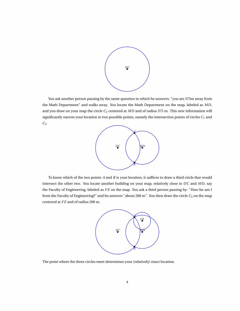
Imagine you are lost on campus, you are holding a campus map in your hand but it does not help much.

You ask someone on campus: "Where am I?" and the person answers "you are 500m away from the uni-

versity center" and he walks away. You locate the university center, labeled as UC on the campus map,

but that does help much since you could be anywhere on the circle C1 centered at UC and of radius 500

m. You draw C1 using the scaling of the campus map.

3

UC

You ask another person passing by the same question to which he answers: "you are 375m away from

the Math Department" and walks away. You locate the Math Department on the map, labeled as MD,

and you draw on your map the circle C2 centered at MD and of radius 375 m. This new information will

significantly narrow your location to two possible points, namely the intersection points of circles C1 and

C2.

MDUC

A

B

To know which of the two points A and B is your location, it suffices to draw a third circle that would

intersect the other two. You locate another building on your map, relatively close to UC and MD, say

the Faculty of Engineering, labeled as F E on the map. You ask a third person passing by: "How far am I

from the Faculty of Engineering?" and he answers "about 200 m". You then draw the circle C3 on the map

centered at F E and of radius 200 m.

MDUC

A

B

F E

The point where the three circles meet determines your (relatively) exact location.

4

Of course, in order for this to work, you must be lucky enough to have people passing by giving you (rel-

atively) precise distances from various locations and to be able to somehow work the scale of the map to

draw (relatively) accurate circles. What is probably more important is the kind of question you should ask

the third person in order to endure that the third circle will somehow meet the other two at at exactly one

point.

3.2 Where am I on the surface of the Planet?

A GPS receiver works the same way except in three dimensions and the friendly people you asked to pin-

point your position on the campus map are replaced with satellites thousands of kilometers above the

surface of the Earth continually emitting signals with crucial data stored in them.

The GPS satellite signal is a digital signal similar to the "noise" you hear on the radio when you cannot

tune in the correct station. A civilian GPS signal contains three different parts:

• A pseudo-random code, a sort of identification code that tells helps the receiver knowing which one

of which one of the active satellites is transmitting the signal;

• An ephemeris data, which is the part of the signal that tells the receiver where the satellite should

be at any time throughout the day. It basically contains detailed information about the orbit of that

particular satellite only and the current date and time according to the (atomic) clock on board of

the satellite. This is vital for the operation of the GPS receiver.

• An almanac data which informs the GPS receiver where each GPS satellite should be at any time.

Each satellite emits almanac data about its own orbit as well as other active satellite in the GPS

constellation.

3.2.1 Measuring the distance to a satellite

Now for the story of locating the position on the surface of the planet.

Signals transmitted by GPS satellites move at the speed of light (in a vacuum) and reach a GPS receiver

at slightly different times as some satellites are further away from the receiver than others. Once the re-

ceiver captures a signal, it immediately recognizes which satellite it is coming from, the start time ω (the

time at which the signal left the satellite according to the satellite clock) and the period of a cycle in the

captured signal. The receiver internal computer starts to "play" the same pseudo-random sequence of

that satellite (using an almanac data stored in the receiver memory) at the same time ω. The two signals

will not generally match and there will be some lag due to travel time d t taken by the satellite signal in

space to reach the receiver. By comparing how late the satellite’s pseudo-random code appears compared

to our receiver’s code, we can determine the time d t it took the signal to reach the receiver.

5

Does this seem to be a bit too technical? the next paragraph will try to explain the idea of the "time

lag" using a simple example.

Let us assume that a GPS satellite signal is just a "song" broadcasted by the satellite. Imagine that at 6:00

am, a GPS satellite begins to broadcast the song

"I see trees of green, red roses too, I see them bloom for me and you..."

in the form of a radio wave to Earth. At the same time (6:00pm), a GPS receiver starts playing the same

song. After traveling thousands of kilometers in space, the radio wave arrives at the receiver but with a

certain delay in the words. At the time of signal reception, if you are holding the receiver in your hand, you

will hear two versions of the song at the same time: the receiver version is playing "...them bloom for..." but

the satellite version is playing (for instance) the first "I see...". The receiver player would then immediately

"rewind" its version a bit until it synchronizes perfectly with the received version. The amount of time

equivalent to this "shift back" in the receiver player is precisely the travel time of the satellite’s version.

Once the time delay d t (in seconds) is computed, the receiver computer would multiply it with the

speed of light (in vacuum), c = 299,792,458m/sec to calculate the distance separating the satellite from

the GPS receiver.

Now that we have a bit more understanding of how the GPS estimates its distance to the satellites in

its view, it is time to see how these estimates are put in use to pinpoint the position of the receiver.

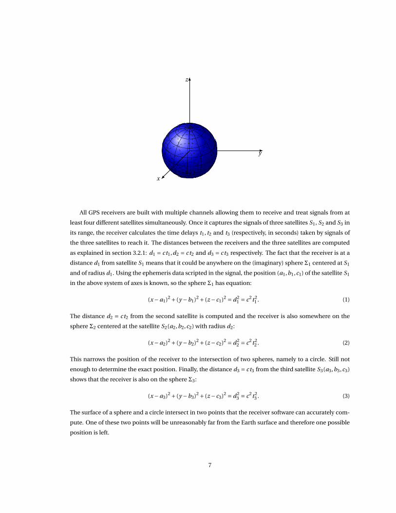
We start by choosing a system of three coordinates axes with the center of the Earth as center of the

system. As usual, the z-axis is the vertical one passing through the two poles and oriented from South

to North. The xz plane is the Greenwich meridian plane. The x-axis lies in the equatorial plane and the

direction of positive values of x goes through the Greenwich point (point of longitude zero). Similarly,

The y-axis lies in the equatorial plane and the direction of positive values of y goes through the point of

longitude 90◦ East.

6

y

z

x

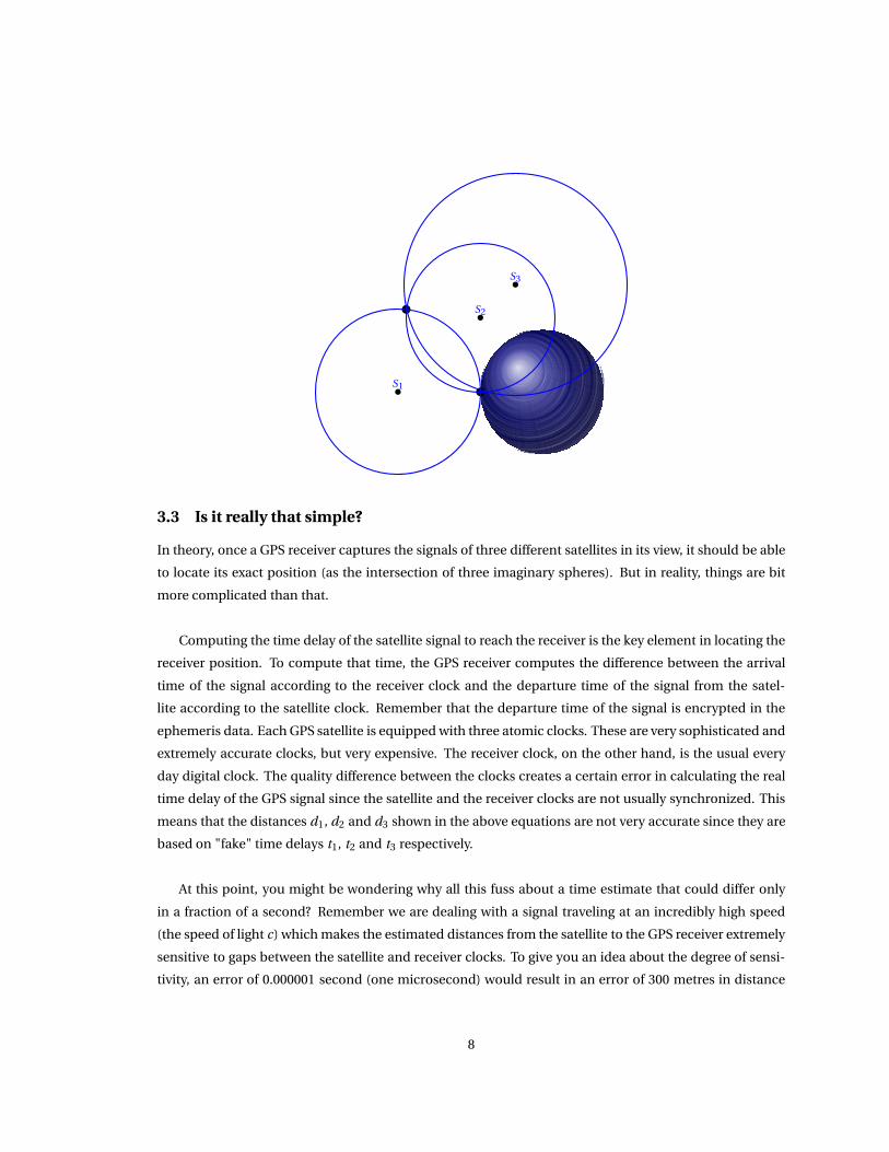
All GPS receivers are built with multiple channels allowing them to receive and treat signals from at

least four different satellites simultaneously. Once it captures the signals of three satellites S1, S2 and S3 in

its range, the receiver calculates the time delays t1, t2 and t3 (respectively, in seconds) taken by signals of

the three satellites to reach it. The distances between the receivers and the three satellites are computed

as explained in section 3.2.1: d1 = ct1,d2 = ct2 and d3 = ct3 respectively. The fact that the receiver is at a

distance d1 from satellite S1 means that it could be anywhere on the (imaginary) sphere Σ1 centered at S1

and of radius d1. Using the ephemeris data scripted in the signal, the position (a1,b1,c1) of the satellite S1

in the above system of axes is known, so the sphere Σ1 has equation:

(x −a1)2 + (y −b1)2 + (z −c1)2 = d21 = c2t 2

1 . (1)

The distance d2 = ct2 from the second satellite is computed and the receiver is also somewhere on the

sphere Σ2 centered at the satellite S2(a2,b2,c2) with radius d2:

(x −a2)2 + (y −b2)2 + (z −c2)2 = d22 = c2t 2

2 . (2)

This narrows the position of the receiver to the intersection of two spheres, namely to a circle. Still not

enough to determine the exact position. Finally, the distance d3 = ct3 from the third satellite S3(a3,b3,c3)

shows that the receiver is also on the sphere Σ3:

(x −a3)2 + (y −b3)2 + (z −c3)2 = d23 = c2t 2

3 . (3)

The surface of a sphere and a circle intersect in two points that the receiver software can accurately com-

pute. One of these two points will be unreasonably far from the Earth surface and therefore one possible

position is left.

7

S1

S2

S3

3.3 Is it really that simple?

In theory, once a GPS receiver captures the signals of three different satellites in its view, it should be able

to locate its exact position (as the intersection of three imaginary spheres). But in reality, things are bit

more complicated than that.

Computing the time delay of the satellite signal to reach the receiver is the key element in locating the

receiver position. To compute that time, the GPS receiver computes the difference between the arrival

time of the signal according to the receiver clock and the departure time of the signal from the satel-

lite according to the satellite clock. Remember that the departure time of the signal is encrypted in the

ephemeris data. Each GPS satellite is equipped with three atomic clocks. These are very sophisticated and

extremely accurate clocks, but very expensive. The receiver clock, on the other hand, is the usual every

day digital clock. The quality difference between the clocks creates a certain error in calculating the real

time delay of the GPS signal since the satellite and the receiver clocks are not usually synchronized. This

means that the distances d1, d2 and d3 shown in the above equations are not very accurate since they are

based on "fake" time delays t1, t2 and t3 respectively.

At this point, you might be wondering why all this fuss about a time estimate that could differ only

in a fraction of a second? Remember we are dealing with a signal traveling at an incredibly high speed

(the speed of light c) which makes the estimated distances from the satellite to the GPS receiver extremely

sensitive to gaps between the satellite and receiver clocks. To give you an idea about the degree of sensi-

tivity, an error of 0.000001 second (one microsecond) would result in an error of 300 metres in distance

8

estimation. No wonder why the GPS receiver’s clock is the main source of error.

The main reason we need these expensive atomic clocks on board of the GPS satellites is to make sure

that they are always in perfect synchronization with each other. A consequence of this is that the "time

error" ξ calculated by the receiver is the same for any satellite. Let me explain: if ξ1 is the time of reception

of the signal according to the receiver clock and if ξ2 is the time of reception of the signal according to the

satellite clock, then ξ= ξ1 −ξ2 is the "time error". Since at any given moment, all satellites read the same

time in their atomic clocks, this time error represents the time difference between the receiver clock and

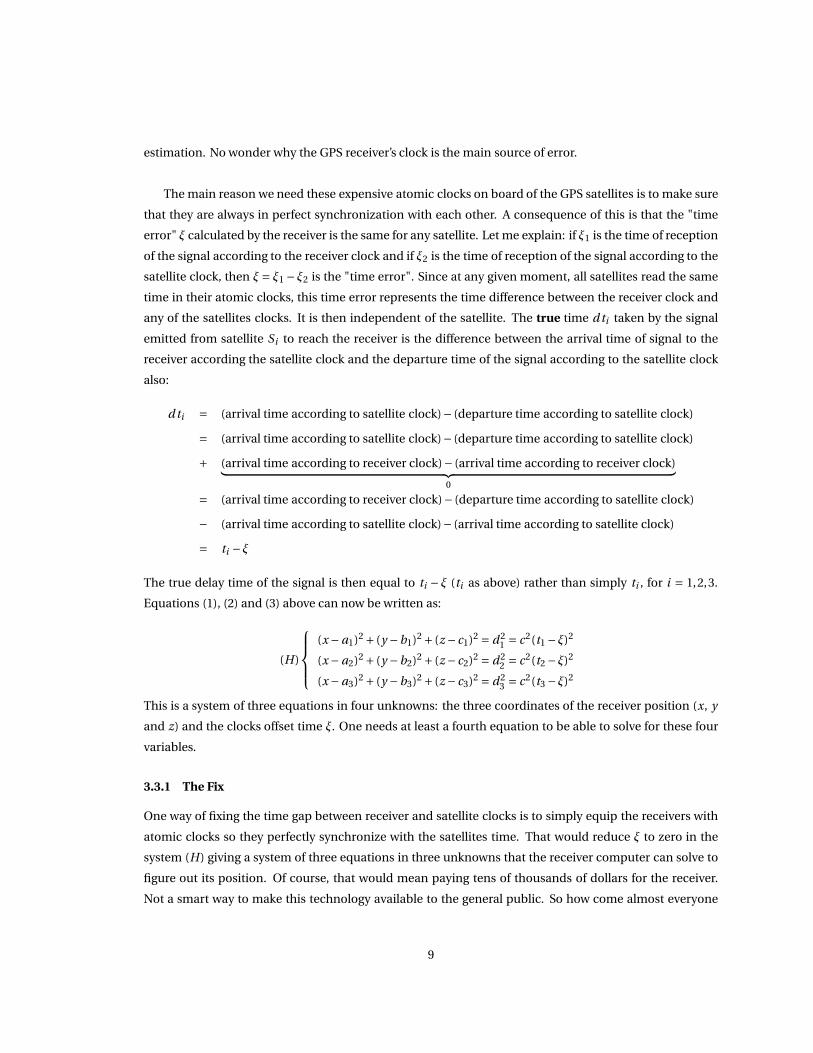
any of the satellites clocks. It is then independent of the satellite. The true time d ti taken by the signal

emitted from satellite Si to reach the receiver is the difference between the arrival time of signal to the

receiver according the satellite clock and the departure time of the signal according to the satellite clock

also:

d ti = (arrival time according to satellite clock)− (departure time according to satellite clock)

= (arrival time according to satellite clock)− (departure time according to satellite clock)

+ (arrival time according to receiver clock)− (arrival time according to receiver clock)︸ ︷︷ ︸

0

= (arrival time according to receiver clock)− (departure time according to satellite clock)

− (arrival time according to satellite clock)− (arrival time according to satellite clock)

= ti −ξ

The true delay time of the signal is then equal to ti − ξ (ti as above) rather than simply ti , for i = 1,2,3.

Equations (1), (2) and (3) above can now be written as:

(H)

(x −a1)2 + (y −b1)2 + (z −c1)2 = d21 = c2(t1 −ξ)2

(x −a2)2 + (y −b2)2 + (z −c2)2 = d22 = c2(t2 −ξ)2

(x −a3)2 + (y −b3)2 + (z −c3)2 = d23 = c2(t3 −ξ)2

This is a system of three equations in four unknowns: the three coordinates of the receiver position (x, y

and z) and the clocks offset time ξ. One needs at least a fourth equation to be able to solve for these four

variables.

3.3.1 The Fix

One way of fixing the time gap between receiver and satellite clocks is to simply equip the receivers with

atomic clocks so they perfectly synchronize with the satellites time. That would reduce ξ to zero in the

system (H) giving a system of three equations in three unknowns that the receiver computer can solve to

figure out its position. Of course, that would mean paying tens of thousands of dollars for the receiver.

Not a smart way to make this technology available to the general public. So how come almost everyone

9

you know has a very affordable GPS receiver that is very accurate at the same time?

The answer is in the mathematically brilliant idea the designers of the GPS came up with. As it turns

out, a simple digital clock in your GPS receiver will do just fine and all what it take is one more measure-

ment from a fourth satellite and voilà, you have an atomic clock right in the palm of your hand.

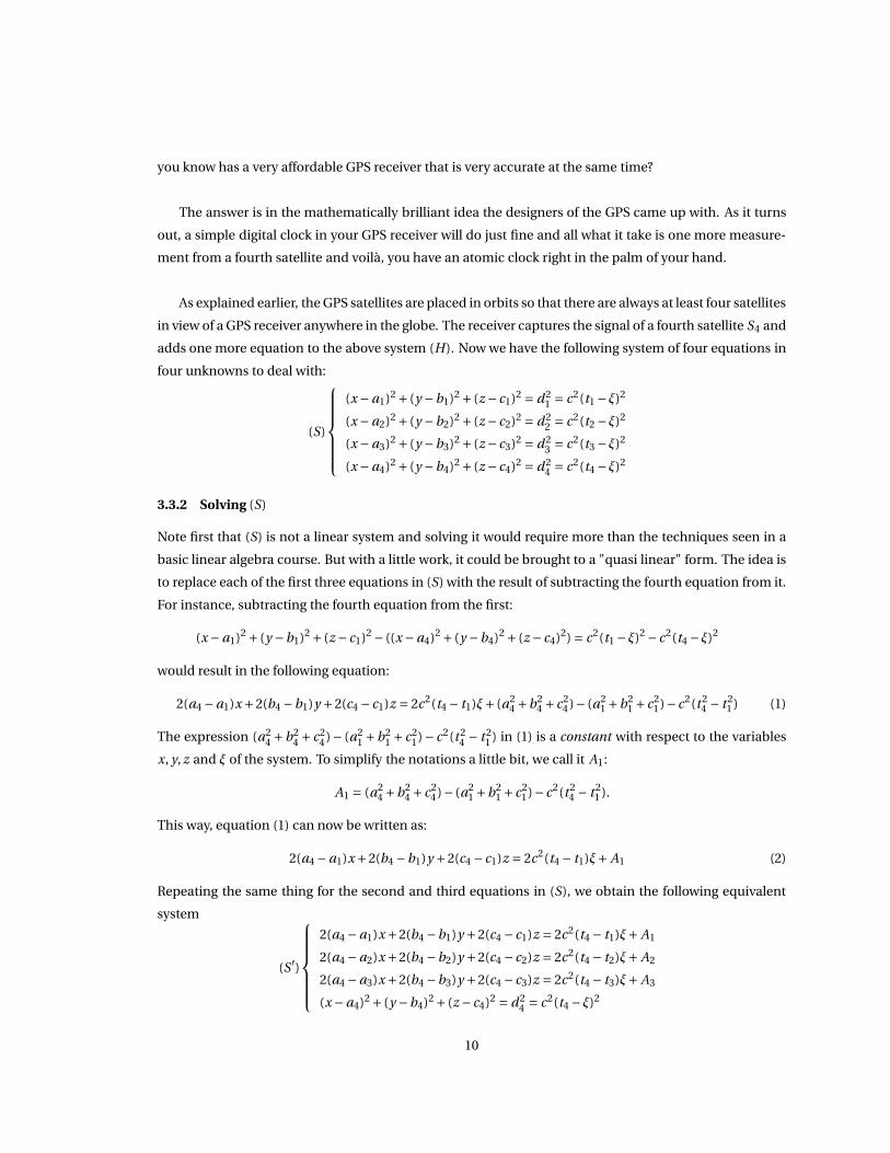
As explained earlier, the GPS satellites are placed in orbits so that there are always at least four satellites

in view of a GPS receiver anywhere in the globe. The receiver captures the signal of a fourth satellite S4 and

adds one more equation to the above system (H). Now we have the following system of four equations in

four unknowns to deal with:

(S)

(x −a1)2 + (y −b1)2 + (z −c1)2 = d21 = c2(t1 −ξ)2

(x −a2)2 + (y −b2)2 + (z −c2)2 = d22 = c2(t2 −ξ)2

(x −a3)2 + (y −b3)2 + (z −c3)2 = d23 = c2(t3 −ξ)2

(x −a4)2 + (y −b4)2 + (z −c4)2 = d24 = c2(t4 −ξ)2

3.3.2 Solving (S)

Note first that (S) is not a linear system and solving it would require more than the techniques seen in a

basic linear algebra course. But with a little work, it could be brought to a "quasi linear" form. The idea is

to replace each of the first three equations in (S) with the result of subtracting the fourth equation from it.

For instance, subtracting the fourth equation from the first:

(x −a1)2 + (y −b1)2 + (z −c1)2 − ((x −a4)2 + (y −b4)2 + (z −c4)2) = c2(t1 −ξ)2 −c2(t4 −ξ)2

would result in the following equation:

2(a4 −a1)x +2(b4 −b1)y +2(c4 −c1)z = 2c2(t4 − t1)ξ+ (a24 +b2

4 +c24 )− (a2

1 +b21 +c2

1 )−c2(t 24 − t 2

1 ) (1)

The expression (a24 +b2

4 + c24 )− (a2

1 +b21 + c2

1)− c2(t 24 − t 2

1 ) in (1) is a constant with respect to the variables

x, y, z and ξ of the system. To simplify the notations a little bit, we call it A1:

A1 = (a24 +b2

4 +c24 )− (a2

1 +b21 +c2

1)−c2(t 24 − t 2

1 ).

This way, equation (1) can now be written as:

2(a4 −a1)x +2(b4 −b1)y +2(c4 −c1)z = 2c2(t4 − t1)ξ+ A1 (2)

Repeating the same thing for the second and third equations in (S), we obtain the following equivalent

system

(S ′)

2(a4 −a1)x +2(b4 −b1)y +2(c4 −c1)z = 2c2(t4 − t1)ξ+ A1

2(a4 −a2)x +2(b4 −b2)y +2(c4 −c2)z = 2c2(t4 − t2)ξ+ A2

2(a4 −a3)x +2(b4 −b3)y +2(c4 −c3)z = 2c2(t4 − t3)ξ+ A3

(x −a4)2 + (y −b4)2 + (z −c4)2 = d24 = c2(t4 −ξ)2

10

One way to solve (S ′) is to treat ξ as a constant in each of the first three equations. This will allow us to

express each of the variables x, y and z in terms of ξ and then use the fourth equation to find ξ (hence

x, y and z). This approach enables us to use the techniques of Linear algebra to solve systems of linear

equations since the first three equations in (S ′) form indeed a system of three linear equations in three

variables (x, y and z).

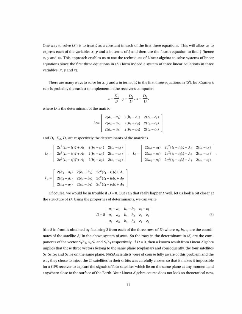
There are many ways to solve for x, y and z in term of ξ in the first three equations in (S ′), but Cramer’s

rule is probably the easiest to implement in the receiver’s computer:

x =D1

D, y =

D2

D, z =

D3

D,

where D is the determinant of the matrix:

L :=

2(a4 −a1) 2(b4 −b1) 2(c4 −c1)

2(a4 −a2) 2(b4 −b2) 2(c4 −c2)

2(a4 −a3) 2(b4 −b3) 2(c4 −c3)

and D1, D2, D3 are respectively the determinants of the matrices

L1 =

2c2(t4 − t1)ξ+ A1 2(b4 −b1) 2(c4 −c1)

2c2(t4 − t2)ξ+ A2 2(b4 −b2) 2(c4 −c2)

2c2(t4 − t3)ξ+ A3 2(b4 −b3) 2(c4 −c3)

, L2 =

2(a4 −a1) 2c2(t4 − t1)ξ+ A1 2(c4 −c1)

2(a4 −a2) 2c2(t4 − t2)ξ+ A2 2(c4 −c2)

2(a4 −a3) 2c2(t4 − t3)ξ+ A3 2(c4 −c3)

,

L3 =

2(a4 −a1) 2(b4 −b1) 2c2(t4 − t1)ξ+ A1

2(a4 −a2) 2(b4 −b2) 2c2(t4 − t2)ξ+ A2

2(a4 −a3) 2(b4 −b3) 2c2(t4 − t3)ξ+ A3

Of course, we would be in trouble if D = 0. But can that really happen? Well, let us look a bit closer at

the structure of D. Using the properties of determinants, we can write

D = 8

∣∣∣∣∣∣∣∣

a4 −a1 b4 −b1 c4 −c1

a4 −a2 b4 −b2 c4 −c2

a4 −a3 b4 −b3 c4 −c3

∣∣∣∣∣∣∣∣

(3)

(the 8 in front is obtained by factoring 2 from each of the three rows of D) where ai ,bi ,ci are the coordi-

nates of the satellite Si in the above system of axes. So the rows in the determinant in (3) are the com-

ponents of the vector ~S1S4, ~S2S4 and ~S3S4 respectively. If D = 0, then a known result from Linear Algebra

implies that these three vectors belong to the same plane (coplanar) and consequently, the four satellites

S1,S2,S3 and S4 lie on the same plane. NASA scientists were of course fully aware of this problem and the

way they chose to inject the 24 satellites in their orbits was carefully chosen so that it makes it impossible

for a GPS receiver to capture the signals of four satellites which lie on the same plane at any moment and

anywhere close to the surface of the Earth. Your Linear Algebra course does not look so theocratical now,

11

does it?

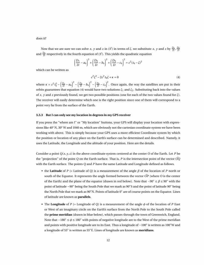
Now that we are sure we can solve x, y and z in (S ′) in terms of ξ, we substitute x, y and z byD1

D,

D2

D

andD3

D respectively in the fourth equation of (S ′). This yields the quadratic equation

(D1

D−a4

)2

+(

D2

D−b4

)2

+(

D3

D−c4

)2

= c2(t4 −ξ)2

which can be written as

c2ξ2 −2c2t4ξ+κ= 0 (4)

where κ = c2t 24 −

(D1

D−a4

)2−

(D2

D−b4

)2−

(D3

D−c4

)2. Once again, the way the satellites are put in their

orbits guarantees that equation (4) would have two solutions ξ1 and ξ2. Substituting back into the values

of x, y and z previously found, we get two possible positions (one for each of the two values found for ξ).

The receiver will easily determine which one is the right position since one of them will correspond to a

point very far from the surface of the Earth.

3.3.3 But I can only see my location in degrees in my GPS receiver

If you press the "where am I" or "My location" buttons, your GPS will display your location with expres-

sions like 40° N, 30° W and 1040 m, which are obviously not the cartesian coordinate system we have been

working with above. This is simply because your GPS uses a more efficient Coordinate system by which

the position or location of any place on the Earth’s surface can be determined and described. Namely, it

uses the Latitude, the Longitude and the altitude of your position. Here are the details.

Consider a point Q(x, y, z) in the above coordinate system centered at the center O of the Earth. Let P be

the "projection" of the point Q on the Earth surface. That is, P is the intersection point of the vector ~OQ

with the Earth surface. The points Q and P have the same Latitude and Longitude defined as follows.

• the Latitude of P (= Latitude of Q) is a measurement of the angle β of the location of P north or

south of the Equator. It represents the angle formed between the vector ~OP (where O is the center

of the Earth) and the plane of the equator (drawn in red below). Note that −90◦ ≤ β ≤ 90◦ with the

point of latitude −90◦ being the South Pole that we mark as 90◦S and the point of latitude 90◦ being

the North Pole that we mark as 90◦N. Points of latitude 0◦ are of course points on the Equator. Lines

of latitude are known as parallels.

• The Longitude of P (= Longitude of Q) is a measurement of the angle φ of the location of P East

or West of an imaginary circle on the Earth’s surface from the North Pole to the South Pole called

the prime meridian (drawn in blue below), which passes through the town of Greenwich, England.

Note that −180◦ ≤φ≤ 180◦ with points of negative longitude are to the West of the prime meridian

and points with positive longitude are to its East. Thus a longitude of −100◦ is written as 100◦W and

a longitude of 55◦ is written as 55◦E. Lines of longitude are known as meridians.

12

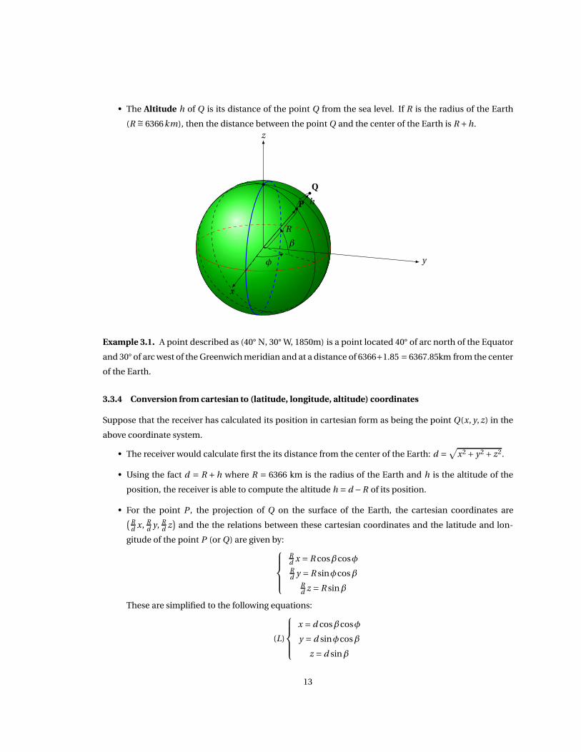
• The Altitude h of Q is its distance of the point Q from the sea level. If R is the radius of the Earth

(R ∼= 6366km), then the distance between the point Q and the center of the Earth is R +h.

x

y

z

P

Q

β

φ

R

h

Example 3.1. A point described as (40° N, 30° W, 1850m) is a point located 40° of arc north of the Equator

and 30° of arc west of the Greenwich meridian and at a distance of 6366+1.85 = 6367.85km from the center

of the Earth.

3.3.4 Conversion from cartesian to (latitude, longitude, altitude) coordinates

Suppose that the receiver has calculated its position in cartesian form as being the point Q(x, y, z) in the

above coordinate system.

• The receiver would calculate first the its distance from the center of the Earth: d =√

x2 + y2 + z2.

• Using the fact d = R +h where R = 6366 km is the radius of the Earth and h is the altitude of the

position, the receiver is able to compute the altitude h = d −R of its position.

• For the point P , the projection of Q on the surface of the Earth, the cartesian coordinates are(

Rd

x, Rd

y, Rd

z)

and the the relations between these cartesian coordinates and the latitude and lon-

gitude of the point P (or Q) are given by:

Rd x = R cosβcosφ

Rd

y = R sinφcosβ

Rd z = R sinβ

These are simplified to the following equations:

(L)

x = d cosβcosφ

y = d sinφcosβ

z = d sinβ

13

The last equation gives that sinβ= zd

and since −90◦ ≤β≤ 90◦, there is a unique value ofβ satisfying

sinβ= zd , namely β= arcsin

(zd

)

.

• Replacing β with arcsin(

zd

)

in the first two equations of the system (L) above reduces the system to

the following two equations:{

cosφ= xd cosβ

sinφ= yd cosβ

with cosβ known. Since −180◦ ≤φ≤ 180◦, these two equations determine uniquely the value of the

longitude φ.

• Thus the position Q(x, y, z) of the receiver can now be displayed in terms of the latitude, longitude

and altitude of the position point Q .

4 The Mathematics of the GPS Signal

Obviously, the satellites are not emitting their signals using the words of the song "I see trees of green red

roses too..." and the receiver does not actually "forward" its version to compute the time gap. So what is

the nature of these signals and how are they engineered to be easily identified by a ground receiver and

more importantly, to be sufficiently "random" to suit the intended use?

Locating the position on (or near) the surface of the Globe using signals from four different satellites

may have appeared somehow complicated to you, but the truth is that this is the "soft" side of Mathemat-

ics used in this project. Careful encryption of codes in the signal emitted by the satellite is key to ensure

accuracy and reliability of information provided by your receiver. This side of the GPS project requires

heavier mathematical tools.

4.1 Linear Feedback Shift Registers

we start with a definition.

Definition 4.1. A binary sequence is sequence of two symbols, normally denoted by of 0 and 1, that we

call bits. A binary sequence is called of length r if it is a finite sequence consisting of r bits. A sequence

a0, a1, a2, . . . is called periodic if there exists a positive integer p, called a period of the sequence, such

that an+p = an for all n. Note that if p is a period, then kp is also a period for any positive integer k. The

smallest possible value for p is called the minimal period of the sequence.

Example 4.1. The sequence

001011000101100010110001011000101100010110001011000101100010110

is a binary sequence of length 63 and periodic of minimal period 7 repeating the block 0010110 of 7 digits.

14

Note that a binary sequence of length r can be expressed as a vector (a0, a1, . . . ar−1) where each com-

ponent ai is an element of F2 := {0, 1}. This means in particular that there are 2.2. . . 2︸ ︷︷ ︸

r

= 2r such sequences.

More formally, we have the following.

Proposition 4.1. There is a total of 2r different binary sequences of length r .

Example 4.2. There are 23 = 8 binary sequences of length 3: 111, 110, 101, 100, 011, 010, 001 and 000.

The codes emitted by GPS satellites (called pseudo-random noise codes, or PRN for short) are treated by

the receivers as "deterministic" binary sequences with noise-like properties. These sequences are "de-

terministic" in the sense that they are not truly random but rather completely determined by a relatively

small set of initial values, called the PRNG’s state. The "G" in "PRNG" stands for "Generator", or more

precisely a "pseudo-random number generator, which is the "Algorithm" used to produce such a deter-

ministic binary sequence.

There are many pseudo-random number generators out there used for various applications. The one

used in producing the pseudo-random codes for satellites is called Linear Feedback Shift Register or

LFSR for short.

In simple terms, a LFSR can be described as a device on board of each satellite for generating a se-

quence of binary bits that has the "appearance" to be very random although it is periodical. Physically, a

LFSR can be represented by a series of r one-bit storage (or memory) cells each containing a bit ak ∈ {0, 1}

and is set by an initial "secret key" consisting of a list of initial r bits: a0, a1, . . . , ar−1.

The behavior of the register is controlled by a counter, often referred to as a “clock”. When a "clock

pulse" is applied, the content of each cell is shifted to the right by one position, reading out the content of

the last (right most) cell. The content in the leftmost cell is the output of certain linear function applied to

the previous state (hence, the word "linear" in the name of that mechanism). The coefficients used in the

linear function to produce the content in the leftmost cell are labeled as c0, c1, . . . ,cr−1. These coefficients

differ from one satellite to another and this is what makes the signal produced by one satellite unique

and different from signals produced by other satellites. This enables the GPS receiver to easily associate a

captured signal with the specific satellite emitting it and to quickly synchronize with it.

Did you find this a bit confusing? No worries, keep reading.

In what follows, we give a step-by-step description of the operating mechanism of a LFSR.

• First, we choose the secret key: a list of r bits: a0, a1, . . . , ar−1 not all zeros at the same time.

• We represent a LFSR by a set of r storage cells, each holding a bit ai ∈ {0,1}. Each cell is connected

15

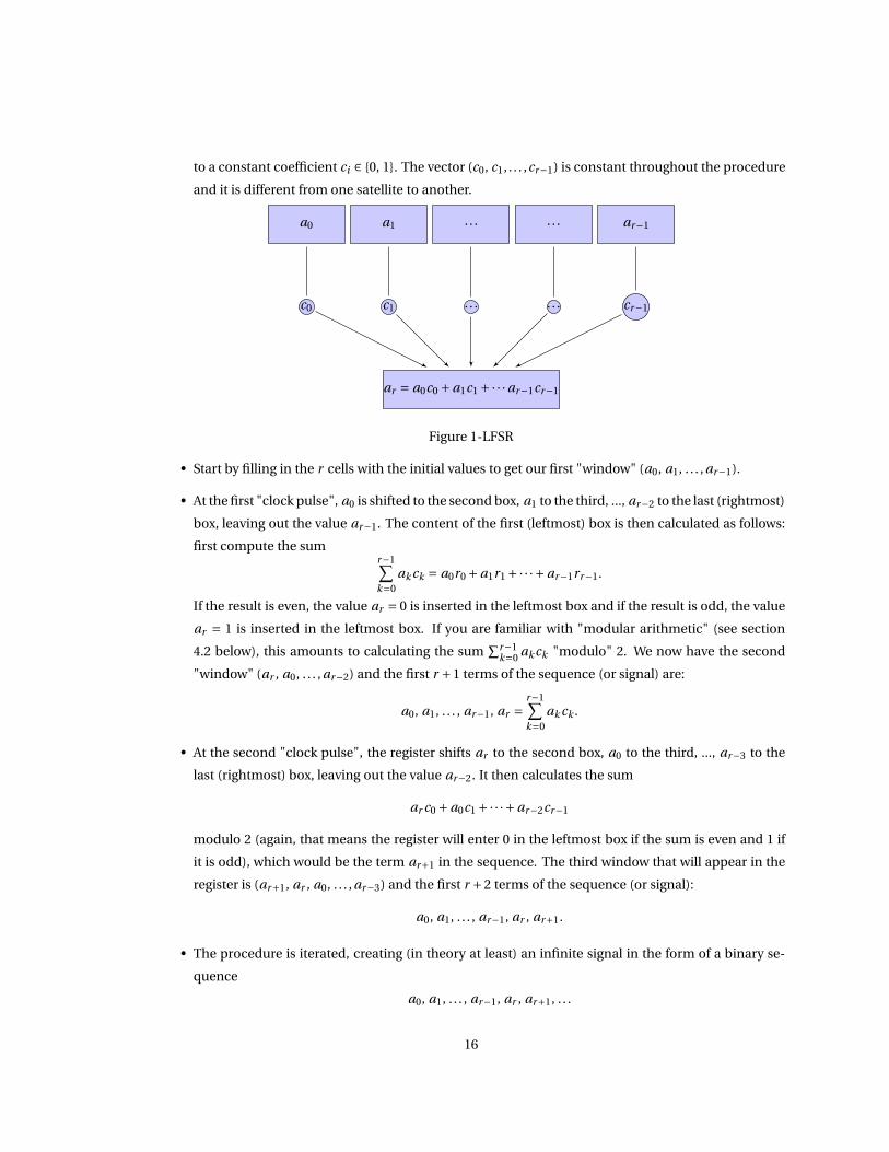
to a constant coefficient ci ∈ {0, 1}. The vector (c0, c1, . . . ,cr−1) is constant throughout the procedure

and it is different from one satellite to another.

a0 a1 . . . . . . ar−1

c0 c1 . . . . . . cr−1

ar = a0c0 +a1c1 +·· ·ar−1cr−1

Figure 1-LFSR

• Start by filling in the r cells with the initial values to get our first "window" (a0, a1, . . . , ar−1).

• At the first "clock pulse", a0 is shifted to the second box, a1 to the third, ..., ar−2 to the last (rightmost)

box, leaving out the value ar−1. The content of the first (leftmost) box is then calculated as follows:

first compute the sumr−1∑

k=0

ak ck = a0r0 +a1r1 +·· ·+ar−1rr−1.

If the result is even, the value ar = 0 is inserted in the leftmost box and if the result is odd, the value

ar = 1 is inserted in the leftmost box. If you are familiar with "modular arithmetic" (see section

4.2 below), this amounts to calculating the sum∑r−1

k=0ak ck "modulo" 2. We now have the second

"window" (ar , a0, . . . , ar−2) and the first r +1 terms of the sequence (or signal) are:

a0, a1, . . . , ar−1, ar =r−1∑

k=0

ak ck .

• At the second "clock pulse", the register shifts ar to the second box, a0 to the third, ..., ar−3 to the

last (rightmost) box, leaving out the value ar−2. It then calculates the sum

ar c0 +a0c1 +·· ·+ar−2cr−1

modulo 2 (again, that means the register will enter 0 in the leftmost box if the sum is even and 1 if

it is odd), which would be the term ar+1 in the sequence. The third window that will appear in the

register is (ar+1, ar , a0, . . . , ar−3) and the first r +2 terms of the sequence (or signal):

a0, a1, . . . , ar−1, ar , ar+1.

• The procedure is iterated, creating (in theory at least) an infinite signal in the form of a binary se-

quence

a0, a1, . . . , ar−1, ar , ar+1, . . .

16

Before we proceed further to look in a bit more depth at the mathematical properties of this sequence,

let us look at a simple example of such a signal.

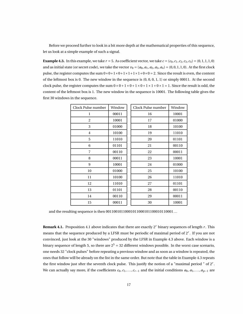
Example 4.3. In this example, we take r = 5. As coefficient vector, we take c = (c0,c1,c2,c3,c4) = (0,1,1,1,0)

and as initial state (or secret code), we take the vector v0 = (a0, a1, a2, a3, a4) = (0,0,1,1,0). At the first clock

pulse, the register computes the sum 0×0+1×0+1×1+1×1+0×0= 2. Since the result is even, the content

of the leftmost box is 0. The new window in the sequence is (0, 0, 0, 1, 1) or simply 00011. At the second

clock pulse, the register computes the sum 0×0+1×0+1×0+1×1+0×1= 1. Since the result is odd, the

content of the leftmost box is 1. The new window in the sequence is 10001. The following table gives the

first 30 windows in the sequence.

Clock Pulse number Window

1 00011

2 10001

3 01000

4 10100

5 11010

6 01101

7 00110

8 00011

9 10001

10 01000

11 10100

12 11010

13 01101

14 00110

15 00011

Clock Pulse number Window

16 10001

17 01000

18 10100

19 11010

20 01101

21 00110

22 00011

23 10001

24 01000

25 10100

26 11010

27 01101

28 00110

29 00011

30 10001

and the resulting sequence is then 00110010110001011000101100010110001. . .

Remark 4.1. Proposition 4.1 above indicates that there are exactly 2r binary sequences of length r . This

means that the sequence produced by a LFSR must be periodic of maximal period of 2r . If you are not

convinced, just look at the 30 "windows" produced by the LFSR in Example 4.3 above. Each window is a

binary sequence of length 5, so there are 25 = 32 different windows possible. In the worst case scenario,

one needs 32 "clock pulses" before repeating a previous window and as soon as a window is repeated, the

ones that follow will be already on the list in the same order. But note that the table in Example 4.3 repeats

the first window just sfter the seventh clock pulse. This justify the notion of a "maximal period " of 2r .

We can actually say more, if the coefficients c0, c1, . . . ,cr−1 and the initial conditions a0, a1, . . . , ap−1 are

17

chosen "wisely" (as we will do in the sequel) we can guarantee that no window of all zeros will ever occur

and that will give us a maximal period of 2r −1.

All the mechanism that we will develop in the following sections are geared toward proving the follow-

ing main main result.

Theorem 4.1. For a LFSR as described above, one can always choose the coefficients c0, c1, . . . ,cr−1 and

initial conditions a0, a1, . . . , ar−1 in such a way that the sequence produced by the register has a minimal

period of exactly 2r −1.

4.2 Some modular Arithmetic

Long Division is a technique that you learnt so early in your student life that you most likely don’t remem-

ber in what grade. The Division Algorithm of integers is a building block for almost every thing we do in

Arithmetic and modular Arithmetic. Let us start by stating this algorithm properly.

Theorem 4.2. (Division Algortitm) Given two integers a and b, with b 6= 0, there exist unique integers q

and r such that a = bq + r and 0≤ r < |b|, where |b| is the absolute value of b.

The integer q is called the quotient, r is called the remainder, b is called the divisor and a is called

the dividend.

For the rest of this section, we fix an integer n ≥ 2.

Definition 4.2. Given two integers a,b ∈ Z, we say that a and b are congruent modulo n and we write

a ≡ b ( mod n), if a and b have the same remainder upon division by n.

If a,b ∈ Z have the same remainder upon division by n, then by the Division Algorithm we can write

a = nq1 + r and b = nq2 + r for some q1, q2 and r ∈ Z with 0 ≤ r < n. So a −b = (nq1 + r )− (nq2 + r ) =n(q1−q2) is divisible by n. Conversely, suppose that a−b =αn is divisible by n and write a = nq1+r1 and

b = nq2+r2 for some q1, q2,r1 and r1 ∈Z with 0 ≤ r1 < n and 0≤ r2 < n. We can clearly assume that r2 ≤ r1

(if not, just inverse the roles of a and b). So, a −b = n(q1 − q2)+ (r1 − r2) = αn. By the uniqueness of the

quotient and the remainder (Theorem 4.2), we conclude that r1 − r2 = 0. In other words, a and b have the

same remainder upon division by n. This proves the following.

Theorem 4.3. For a,b ∈Z, a ≡ b (mod n) if and only if a −b is divisible by n.

Example 4.4. 11 ≡ 21 ( mod 5) since 11 and 21 have the same remainder (namely 1) upon division by 5

(or equivalently, their difference 21−11 = 10 is divisible by 5).

18

There are n possible remainders upon division by n, namely 0,1, . . . ,n − 1. Given any integer a, the

Division Algorithm allows us to write a = nq + r for some q,r ∈ Z with 0 ≤ r ≤ n −1. Since a − r = nq is

divisible by n, we have that a ≡ r ( mod n). This shows that any integer in Z is congruent modulo n to one

of the elements in the set {0,1, . . . ,n−1}. If k ∈ {0,1, . . . ,n−1} is one of the remainders in the division by n,

we consider the set k of all integers having k as remainder upon division by n, that we call an equivalence

class modulo n:

k := { j ∈Z; j ≡ k ( mod n)}.

We then consider the the collection Zn of all equivalence classes modulo n:

Zn :={

k; 0 ≤ k ≤ n−1}

.

Example 4.5. Z3 ={

0, 1, 2}

where

0 = {. . . ,−9,−6,−3,0,2,6,9, . . .}

1 = {. . . ,−8,−5,−2,1,4,7,10, . . .}

2 = {. . . ,−7,−4,−1,2,5,8,11, . . .}

Remark 4.2. In the notation of the equivalence class k used above, the integer k is just one representative

of that class. Any other element of the same class is also a representative. For instance, in the above

example, 1 can also be represented by −1 or by 7. To avoid confusion, the elements of Zn are always

represented in the (standard) form k for 0 ≤ k ≤ n−1. This way, we write 2 instead of 14 in Z3.

We define and addition and a multiplication that we call addition and a multiplication modulo n on

the elements of the set Zn in the following way:

• Addition modulo n. If a, b ∈ Zn , define a +b to be the class represented by the integer a +b. In

other words,

a +b = a +b.

• Multiplication modulo n. If a, b ∈Zn , define a×b (or ab for simplicity) to be the class represented

by the integer a ×b:

a ×b = a ×b.

Since a class in Zn has infinitely many representatives, one has to check that these two operations are

independent of the choice of representatives. This is left as an easy exercise for the reader.

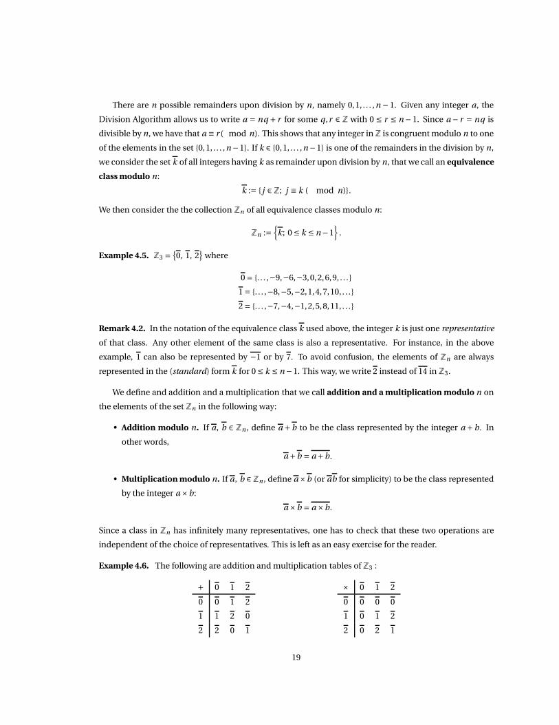
Example 4.6. The following are addition and multiplication tables of Z3 :

+ 0 1 2

0 0 1 2

1 1 2 0

2 2 0 1

× 0 1 2

0 0 0 0

1 0 1 2

2 0 2 1

19

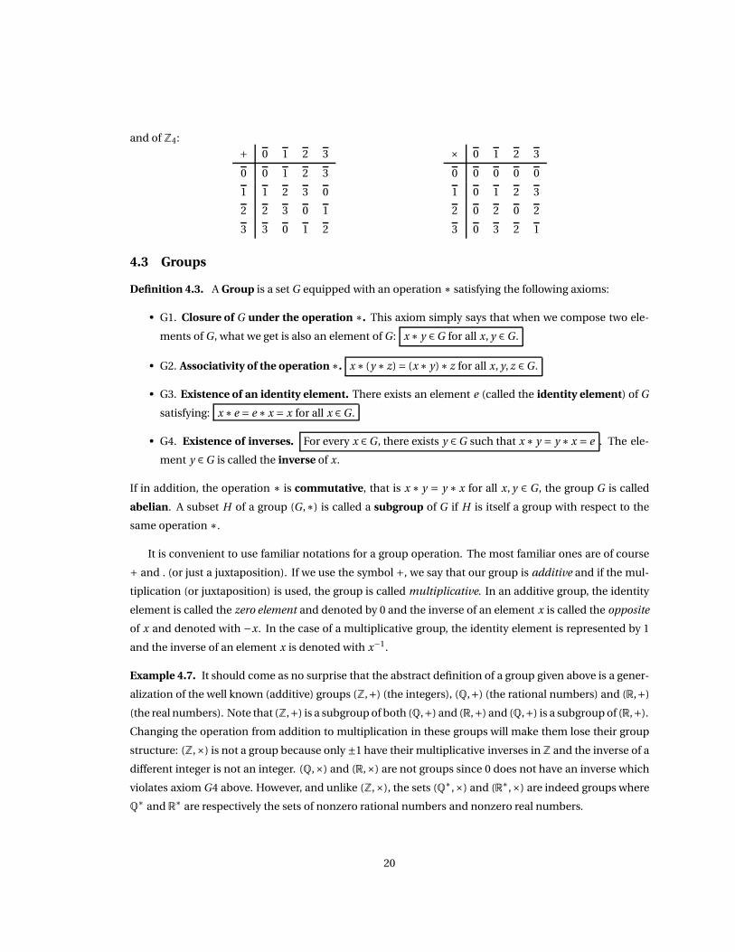
and of Z4:

+ 0 1 2 3

0 0 1 2 3

1 1 2 3 0

2 2 3 0 1

3 3 0 1 2

× 0 1 2 3

0 0 0 0 0

1 0 1 2 3

2 0 2 0 2

3 0 3 2 1

4.3 Groups

Definition 4.3. A Group is a set G equipped with an operation ∗ satisfying the following axioms:

• G1. Closure of G under the operation ∗. This axiom simply says that when we compose two ele-

ments of G, what we get is also an element of G: x ∗ y ∈G for all x, y ∈G.

• G2. Associativity of the operation ∗. x ∗ (y ∗ z)= (x ∗ y)∗ z for all x, y, z ∈G.

• G3. Existence of an identity element. There exists an element e (called the identity element) of G

satisfying: x ∗ e = e ∗ x = x for all x ∈G.

• G4. Existence of inverses. For every x ∈G, there exists y ∈G such that x ∗ y = y ∗ x = e . The ele-

ment y ∈G is called the inverse of x.

If in addition, the operation ∗ is commutative, that is x ∗ y = y ∗ x for all x, y ∈ G, the group G is called

abelian. A subset H of a group (G,∗) is called a subgroup of G if H is itself a group with respect to the

same operation ∗.

It is convenient to use familiar notations for a group operation. The most familiar ones are of course

+ and . (or just a juxtaposition). If we use the symbol +, we say that our group is additive and if the mul-

tiplication (or juxtaposition) is used, the group is called multiplicative. In an additive group, the identity

element is called the zero element and denoted by 0 and the inverse of an element x is called the opposite

of x and denoted with −x. In the case of a multiplicative group, the identity element is represented by 1

and the inverse of an element x is denoted with x−1.

Example 4.7. It should come as no surprise that the abstract definition of a group given above is a gener-

alization of the well known (additive) groups (Z,+) (the integers), (Q,+) (the rational numbers) and (R,+)

(the real numbers). Note that (Z,+) is a subgroup of both (Q,+) and (R,+) and (Q,+) is a subgroup of (R,+).

Changing the operation from addition to multiplication in these groups will make them lose their group

structure: (Z,×) is not a group because only ±1 have their multiplicative inverses in Z and the inverse of a

different integer is not an integer. (Q,×) and (R,×) are not groups since 0 does not have an inverse which

violates axiom G4 above. However, and unlike (Z,×), the sets (Q∗,×) and (R∗,×) are indeed groups where

Q∗ and R∗ are respectively the sets of nonzero rational numbers and nonzero real numbers.

20

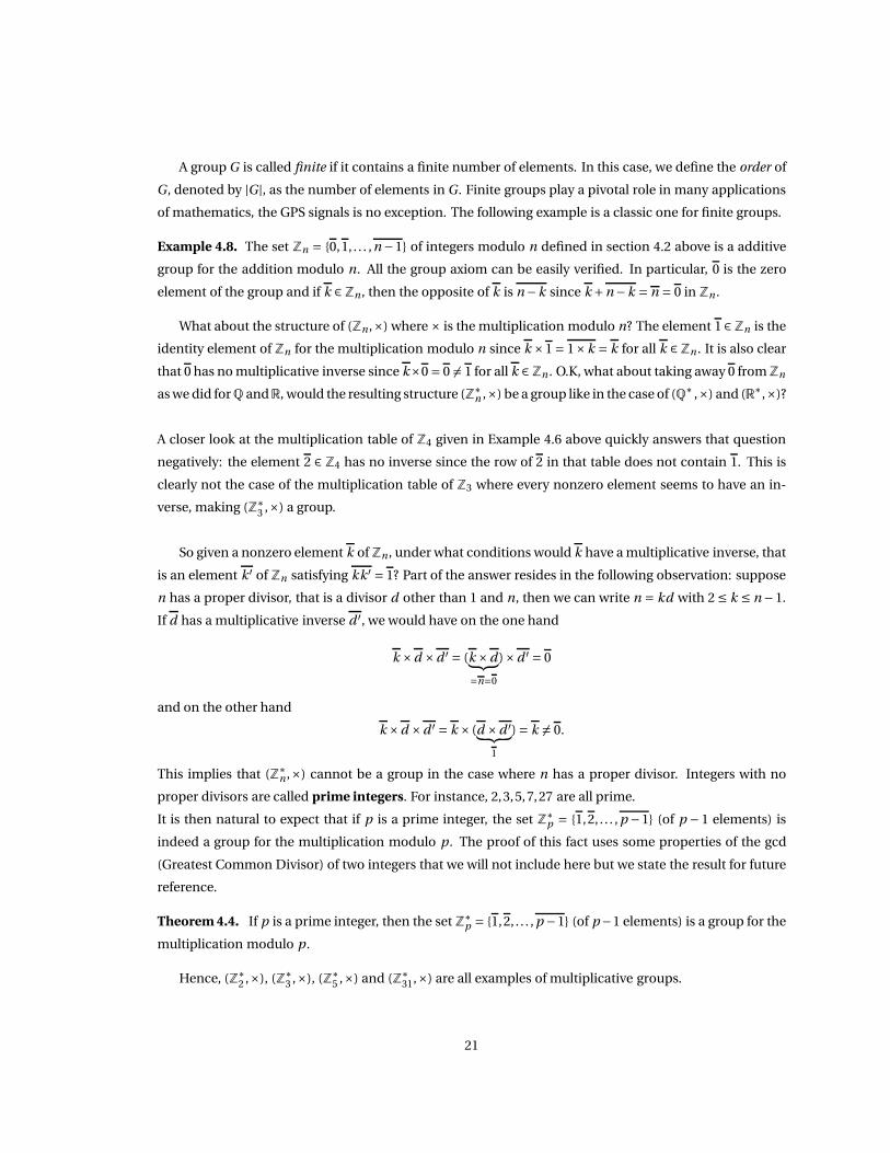
A group G is called finite if it contains a finite number of elements. In this case, we define the order of

G, denoted by |G|, as the number of elements in G. Finite groups play a pivotal role in many applications

of mathematics, the GPS signals is no exception. The following example is a classic one for finite groups.

Example 4.8. The set Zn = {0,1, . . . ,n−1} of integers modulo n defined in section 4.2 above is a additive

group for the addition modulo n. All the group axiom can be easily verified. In particular, 0 is the zero

element of the group and if k ∈Zn , then the opposite of k is n−k since k +n−k = n = 0 in Zn .

What about the structure of (Zn ,×) where × is the multiplication modulo n? The element 1∈Zn is the

identity element of Zn for the multiplication modulo n since k ×1 = 1×k = k for all k ∈Zn . It is also clear

that 0 has no multiplicative inverse since k×0 = 0 6= 1 for all k ∈Zn . O.K, what about taking away 0 fromZn

as we did forQ andR, would the resulting structure (Z∗n ,×) be a group like in the case of (Q∗ ,×) and (R∗,×)?

A closer look at the multiplication table of Z4 given in Example 4.6 above quickly answers that question

negatively: the element 2 ∈ Z4 has no inverse since the row of 2 in that table does not contain 1. This is

clearly not the case of the multiplication table of Z3 where every nonzero element seems to have an in-

verse, making (Z∗3 ,×) a group.

So given a nonzero element k of Zn , under what conditions would k have a multiplicative inverse, that

is an element k ′ of Zn satisfying kk ′ = 1? Part of the answer resides in the following observation: suppose

n has a proper divisor, that is a divisor d other than 1 and n, then we can write n = kd with 2 ≤ k ≤ n−1.

If d has a multiplicative inverse d ′, we would have on the one hand

k ×d ×d ′ = (k ×d︸ ︷︷ ︸

=n=0

)×d ′ = 0

and on the other hand

k ×d ×d ′ = k × (d ×d ′︸ ︷︷ ︸

1

) = k 6= 0.

This implies that (Z∗n ,×) cannot be a group in the case where n has a proper divisor. Integers with no

proper divisors are called prime integers. For instance, 2,3,5,7,27 are all prime.

It is then natural to expect that if p is a prime integer, the set Z∗p = {1,2, . . . , p −1} (of p − 1 elements) is

indeed a group for the multiplication modulo p. The proof of this fact uses some properties of the gcd

(Greatest Common Divisor) of two integers that we will not include here but we state the result for future

reference.

Theorem 4.4. If p is a prime integer, then the set Z∗p = {1,2, . . . , p −1} (of p−1 elements) is a group for the

multiplication modulo p.

Hence, (Z∗2 ,×), (Z∗

3 ,×), (Z∗5 ,×) and (Z∗

31,×) are all examples of multiplicative groups.

21

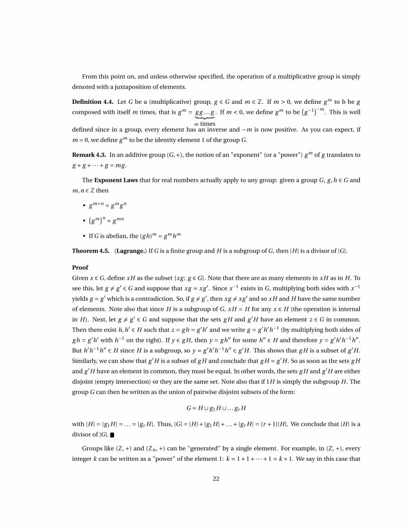
From this point on, and unless otherwise specified, the operation of a multiplicative group is simply

denoted with a juxtaposition of elements.

Definition 4.4. Let G be a (multiplicative) group, g ∈ G and m ∈ Z. If m > 0, we define g m to b be g

composed with itself m times, that is g m = g g . . . g︸ ︷︷ ︸

m times

. If m < 0, we define g m to be(

g−1)−m

. This is well

defined since in a group, every element has an inverse and −m is now positive. As you can expect, if

m = 0, we define g m to be the identity element 1 of the group G.

Remark 4.3. In an additive group (G,+), the notion of an "exponent" (or a "power") g m of g translates to

g + g +·· ·+ g = mg .

The Exponent Laws that for real numbers actually apply to any group: given a group G, g ,h ∈ G and

m,n ∈Z then

• g m+n = g m g n

•(

g m)n = g mn

• If G is abelian, the (g h)m = g mhm

Theorem 4.5. (Lagrange.) If G is a finite group and H is a subgroup of G, then |H | is a divisor of |G|.

Proof

Given x ∈G, define xH as the subset {xg ; g ∈G}. Note that there are as many elements in xH as in H . To

see this, let g 6= g ′ ∈ G and suppose that xg = xg ′. Since x−1 exists in G, multiplying both sides with x−1

yields g = g ′ which is a contradiction. So, if g 6= g ′, then xg 6= xg ′ and so xH and H have the same number

of elements. Note also that since H is a subgroup of G, xH = H for any x ∈ H (the operation is internal

in H). Next, let g 6= g ′ ∈ G and suppose that the sets g H and g ′H have an element z ∈ G in common.

Then there exist h,h′ ∈ H such that z = g h = g ′h′ and we write g = g ′h′h−1 (by multiplying both sides of

g h = g ′h′ with h−1 on the right). If y ∈ g H , then y = g h′′ for some h′′ ∈ H and therefore y = g ′h′h−1h′′.

But h′h−1h′′ ∈ H since H is a subgroup, so y = g ′h′h−1h′′ ∈ g ′H . This shows that g H is a subset of g ′H .

Similarly, we can show that g ′H is a subset of g H and conclude that g H = g ′H . So as soon as the sets g H

and g ′H have an element in common, they must be equal. In other words, the sets g H and g ′H are either

disjoint (empty intersection) or they are the same set. Note also that if 1H is simply the subgroup H . The

group G can then be written as the union of pairwise disjoint subsets of the form:

G = H ∪ g1H ∪ . . . gr H

with |H | = |g1H | = . . . = |gr H |. Thus, |G| = |H |+ |g1 H |+ . . .+|gr H | = (r +1)|H |. We conclude that |H | is a

divisor of |G|.

Groups like (Z, +) and (Zn , +) can be "generated" by a single element. For example, in (Z, +), every

integer k can be written as a "power" of the element 1: k = 1+1+·· · +1 = k ×1. We say in this case that

22

the additive group Z is generated by 1. Note also that −1 is a generator of (Z, +). In general, we have the

following.

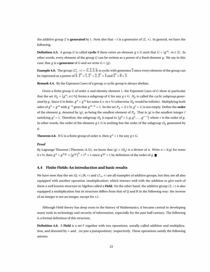
Definition 4.5. A group G is called cyclic if there exists an element g ∈ G such that G = {g m ; m ∈ Z}. In

other words, every element of the group G can be written as a power of a fixed element g . We say in this

case, that g is a generator of G and we write G = ⟨g ⟩.

Example 4.9. The group (Z∗7 , ×) = {1,2,3,4} is cyclic with generator 2 since every element of the group can

be expressed as a power of 4: 20 = 1, 2

1 = 2, 22 = 4 and 2

3 = 8 = 3.

Remark 4.4. By the Exponent Laws of a group, a cyclic group is always abelian.

Given a finite group G of order n and identity element 1, the Exponent Laws of G show in particular

that the set Hg ={

g n ; n ∈N}

forms a subgroup of G for any g ∈G. Hg is called the cyclic subgroup gener-

ated by g . Since G is finite, g k = g m for some k ≤ m ∈N (otherwise Hg would be infinite). Multiplying both

sides of g k = g m with g−k gives that g m−k = 1. So the set Pg = {l ∈N; g l = 1} is not empty. Define the order

of the element g , denoted by |g |, as being the smallest element of Pg . That is |g | is the smallest integer l

satisfying g l = 1. Therefore, the subgroup Hg is equal to{

g 0 = 1, g , g 2, . . . , g r−1}

where r is the order of g .

In other words, the order of the element g ∈ G is nothing but the order of the subgroup Hg generated by

g .

Theorem 4.6. If G is a finite group of order n, then g n = 1 for any g ∈G.

Proof

By Lagrange Theorem (Theorem (4.5)), we know that |g | = |Hg | is a divisor of n. Write n = k|g | for some

k ∈N, then g n = g k |g | =(

g |g |)k = 1k = 1 since g |g | = 1 by definition of the order of g .

4.4 Finite Fields-An introduction and basic results

We have seen that the set (Q,+),(R,+) and (Zn ,+) are all examples of additive groups, but they are all also

equipped with another operation (multiplication) which interact well with the addition to give each of

them a well known structure in Algebra called a Field. On the other hand, the additive group (Z,+) is also

equipped a multiplication but its structure differs from that of Q and R in the following way: the inverse

of an integer is not an integer, except for ±1.

Although Field theory has deep roots in the history of Mathematics, it became central in developing

many tools in technology and security of information, especially for the past half century. The following

is a formal definition of this structure.

Definition 4.6. A Field is a set F together with two operations, usually called addition and multiplica-

tion, and denoted by + and . (or just a juxtaposition), respectively. These operations satisfy the following

axioms:

23

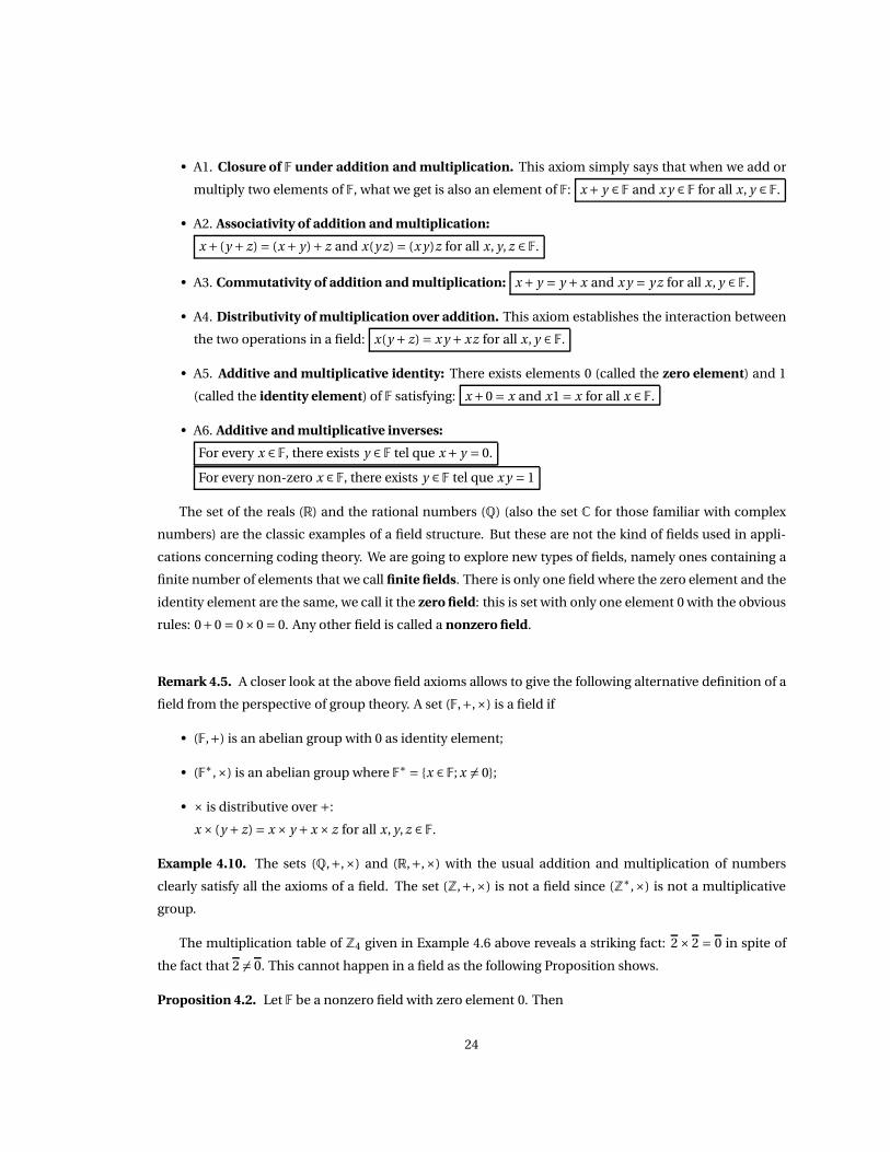
• A1. Closure of F under addition and multiplication. This axiom simply says that when we add or

multiply two elements of F, what we get is also an element of F: x + y ∈ F and x y ∈ F for all x, y ∈ F.

• A2. Associativity of addition and multiplication:

x + (y + z) = (x + y)+ z and x(y z) = (x y)z for all x, y, z ∈ F.

• A3. Commutativity of addition and multiplication: x + y = y + x and x y = y z for all x, y ∈ F.

• A4. Distributivity of multiplication over addition. This axiom establishes the interaction between

the two operations in a field: x(y + z) = x y + xz for all x, y ∈ F.

• A5. Additive and multiplicative identity: There exists elements 0 (called the zero element) and 1

(called the identity element) of F satisfying: x +0 = x and x1 = x for all x ∈ F.

• A6. Additive and multiplicative inverses:

For every x ∈ F, there exists y ∈ F tel que x + y = 0.

For every non-zero x ∈ F, there exists y ∈ F tel que x y = 1

The set of the reals (R) and the rational numbers (Q) (also the set C for those familiar with complex

numbers) are the classic examples of a field structure. But these are not the kind of fields used in appli-

cations concerning coding theory. We are going to explore new types of fields, namely ones containing a

finite number of elements that we call finite fields. There is only one field where the zero element and the

identity element are the same, we call it the zero field: this is set with only one element 0 with the obvious

rules: 0+0 = 0×0 = 0. Any other field is called a nonzero field.

Remark 4.5. A closer look at the above field axioms allows to give the following alternative definition of a

field from the perspective of group theory. A set (F,+,×) is a field if

• (F,+) is an abelian group with 0 as identity element;

• (F∗,×) is an abelian group where F∗ = {x ∈ F; x 6= 0};

• × is distributive over +:

x × (y + z) = x × y + x × z for all x, y, z ∈ F.

Example 4.10. The sets (Q,+,×) and (R,+,×) with the usual addition and multiplication of numbers

clearly satisfy all the axioms of a field. The set (Z,+,×) is not a field since (Z∗,×) is not a multiplicative

group.

The multiplication table of Z4 given in Example 4.6 above reveals a striking fact: 2×2 = 0 in spite of

the fact that 2 6= 0. This cannot happen in a field as the following Proposition shows.

Proposition 4.2. Let F be a nonzero field with zero element 0. Then

24

1. a ×0= 0 for all a ∈ F.

2. If a, b ∈ F are such that a ×b = 0, then either a or b must be zero.

Proof

1. a ×0 = a × (0+0) = a ×0+ a ×0 (by the distributivity property A4 above). As an element of a field,

a ×0 must have an additive inverse −a ×0. Adding −a ×0 to the equation a ×0 = a ×0+a ×0 gives

0= a ×0.

2. Assume a×b = 0. If a 6= 0, then a admits a multiplicative inverse a−1 (axiom A6 above). Multiplying

both sides of the equation a ×b = 0 with a−1 gives

a−1 × (a ×b) = a−1 ×0⇒ (a−1 ×a︸ ︷︷ ︸

1

)×b = 0⇒ 1×b = 0 ⇒ b = 0.

We conclude that at least one of the elements a, b must be zero.

The above proposition, together with the multiplication table of Z4 shows that Z4, equipped with the ad-

dition and the multiplication modulo 4, is not a field since 2×2 = 0 is a violation of part 2 of the above

proposition. On the other hand, addition and multiplication tables of Z3 show that Z3 is indeed a field. In

Z6 we have that 2×3 = 6 = 0 with both 2, 3 are nonzero. It is the fact that 6 can be factored as 2×3 with

1 < 2 < 3< 6 that makes such an equation possible and consequently stops Z6 from being a field.

There is really nothing special about the decomposition 6 = 2×3. In general, if n ≥ 2 is not a prime integer,

then n can be written under the form n = pq where 1 < p, q < n. This translates in Zn into the equation

p×q = n = 0 with both p, q nonzero. This means that Zn is not a field if n is not prime. On the other hand,

Theorem (4.4) above shows that Z∗n is a (multiplicative) if n is a prime integer. We conclude

Theorem 4.7. Zp is a field (for the addition and a multiplication modulo p) if and only if p is a prime

integer.

Hence, Z2, Z5 and Z7 are all examples of finite fields.

Remark 4.6. It can be shown (but we will not show it here) that any finite field F containing p elements

for a prime p is actually a copy of Zp (formally, we say F is isomorphic to Zp ). In other words, there is only

one filed containing p elements for each prime integer p. This field is denoted by Fp .

From this point on, we will omit the "over line" in expressing the element a of Zp and just write a for

simplicity. For instance, we write Z3 = {0,1,2} and Z5 = {0,1,2,3,4}.

25

4.4.1 The field Fpr

The field Zp (or Fp ) containing p elements (for prime p) is just a particular example of a more general

family of finite fields. Given a prime integer p and a positive integer r , the main goal in what follows is

to construct the unique finite field Fpr containing exactly pr elements. Any other field containing pr ele-

ments is just a copy of Fpr .

In all what follows, F is a arbitrary field (not necessarily finite), p is a prime integer and r is a positive

integer. We will "cook" the field Fpr following two recipes. The main ingredient in both recipes is the

notion of polynomials with coefficients in the field F. These are the same type of polynomials that you

always dealt with except that the coefficients are no longer restricted to real numbers.

Definition 4.7. A polynomial in one variable x over F is an expression of the form

p(x) = an xn +an−1xn−1 +·· ·+a1x +a0

where ai ∈ F for each i ∈ {0,1, . . . n}. Moreover, if an 6= 0 (with 0 being the zero element of the field F),

then we say that p(x) is of degree n and we write deg p(x) = n. In this case, the coefficient an is called

the leading coefficient of p(x). A monic polynomial is a polynomial with leading coefficient equal to 1

(the identity element of the field F). If ai = 0 for all i , we say that p(x) is the zero polynomial. The degree

of the zero polynomial is defined to be −∞. Note that any element of the field F can be considered as

a polynomial of degree 0 that we usually call a constant polynomial. The set of all polynomial in one

variable x over F is denoted by F[x].

We define addition and multiplication in F[x] in the usual way of adding and multiplying two polynomials

with the understanding that the involved operations on the coefficients are done in the field F. Equipped

with these two operations, F[x] is clearly not a field since, for example, the multiplicative inverse of the

polynomial p(x) = x does not exist (no polynomial p(x) exists such that xp(x) = 1).

Remark 4.7. We are mainly interested in polynomials over the finite fields Zp (for prime p) and one

has to be careful when computing modulo the prime p. For instance, let p(x) = x2 + x + 1 and q(x) =x +1 considered as polynomials in Z2[x], then p(x)+ q(x) = x2 +2x +2 = x2 since in the filed Z2, 2 = 0

(remember: the coefficient 2 here means 2). Also p(x)q(x)= x3+2x2 +2x+1 = x3+1 for the same reason.

Now, if we consider the same polynomials but as elements of Z3[x], then p(x)+ q(x) = x2 + 2x + 2 and

p(x)q(x)= x3 +2x2 +2x +1.

The notion of divisibly in Z can be extended to F[x] with the understanding that a nonzero polynomial

p(x) is said to divide another polynomial q(x) if q(x) = p(x)k(x) for some k(x) ∈ F[x]. For example, x2 +1

divides x4 −1 since the later is equal to (x2 −1)(x2 +1).

26

Similar to the case of integers, we also have a division algorithm in F[x] usually known as the long division

of polynomials:

Division Algorithm of F[x]. Given two polynomials f (x) and g (x) in F[x] with g (x) 6= 0 and deg g (x) = n,

then uniquely determined polynomials q(x) and r (x) in F[x] exist such that

1. f (x) = g (x)q(x)+ r (x);

2. Either r (x) is the zero polynomial or degr (x) < n.

The polynomial q(x) is called the quotient of the division and r (x) is called the remainder. Note that if

deg f (x) < deg g (x), then we can write f (x) = g (x).0+ f (x) with 0 as quotient and f (x) as remainder.

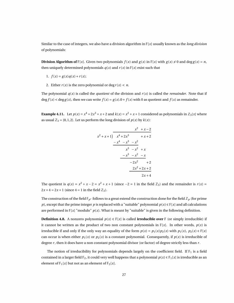
Example 4.11. Let p(x) = x4 +2x3 + x+2 and k(x) = x2 + x+1 considered as polynomials in Z3[x] where

as usual Z3 = {0,1,2}. Let us perform the long division of p(x) by k(x):

x2 + x −2

x2 + x +1)

x4 +2x3 + x +2

− x4 − x3 − x2

x3 − x2 + x

− x3 − x2 − x

−2x2 +2

2x2 +2x +2

2x +4

The quotient is q(x) = x2 + x − 2 = x2 + x + 1 (since −2 = 1 in the field Z3) and the remainder is r (x) =2x +4 = 2x +1 (since 4= 1 in the field Z3).

The construction of the field Fpr follows to a great extend the construction done for the field Zp (for prime

p), except that the prime integer p is replaced with a "suitable" polynomial p(x)∈ F[x] and all calculations

are performed in F[x] "modulo" p(x). What is meant by "suitable" is given in the following definition.

Definition 4.8. A nonzero polynomial p(x) ∈ F[x] is called irreducible over F (or simply irreducible) if

it cannot be written as the product of two non constant polynomials in F[x]. In other words, p(x) is

irreducible if and only if the only way an equality of the form p(x) = p1(x)p2(x) with p1(x), p2(x) ∈ F[x]

can occur is when either p1(x) or p2(x) is a constant polynomial. Consequently, if p(x) is irreducible of

degree r , then it does have a non constant polynomial divisor (or factor) of degree strictly less than r .

The notion of irreducibility for polynomials depends largely on the coefficient field. If F1 is a field

contained in a larger field F2, it could very well happens that a polynomial p(x) ∈ F1[x] is irreducible as an

element of F1[x] but not as an element of F2[x].

27

Example 4.12. The polynomial p(x) = x2 −2 is irreducible as element of Q[x] but not as an element of

R[x] since p(x) = (x −p

2)(x +p

2) and each one of the polynomials (x −p

2), (x +p

2) is non constant in

R[x].

More interesting examples arise in the case of finite fields.

Example 4.13. The polynomial p(x) = x2 +1 is not irreducible over Z2 since (x +1)(x +1) = x2 +2x +1 =x2 +1 in Z2[x]. Note that x2 +1 is clearly irreducible in R[x].

As we did computations "modulo n" in the set Z of all integers, we will define operations "modulo

p(x)" in F[x] for some polynomial p(x) ∈ F[x]. First, a definition.

Definition 4.9. Let F be a field, p(x) ∈ F[x] a nonzero polynomial. We say that the two polynomials

f (x), g (x) ∈ F[x] are congruent modulo p(x), and we write f (x) ≡ g (x) (mod p(x)), if p(x) divides the

difference f (x)− g (x). In many instances, the expression f (x) ≡ g (x) is simply replaced with f (x) = g (x)

(mod p(x)). Note that (like in the case of integers) the fact that p(x) divides f (x)− g (x) is equivalent to

f (x) and g (x) having the same remainder when divided with p(x).

Example 4.14. x3 +2x2 −1 ≡ x2 −1 (mod x +1) in R[x] since x3 +2x2 −1− (x2 −1) = x3 + x2 = x2(x +1).

Example 4.15. x3+3x ≡ x3−x2−2x−1 (mod x2+1) in Z5[x] since x3+3x−(x3−x2−2x−1) = x2+5x+1 =x2 +1 (remember that 5= 0 in Z5).

The division Algorithm is at the heart of computations modulo p(x) in F[x]: If f (x) = g (x)q(x)+r (x), then

f (x)− r (x) = g (x)q(x) and consequently, f (x) ≡ r (x) (mod p(x)). Like in the case of integers modulo n,

given a nonzero polynomial p(x) ∈ F[x] we group the polynomials of F[x] in "classes" according to their

remainder upon division by p(x). So two polynomials f (x) and g (x) are "equal" modulo p(x) if they be-

long to the same class, or equivalently they have the same remainder when divided by p(x).

For a nonzero polynomial p(x) ∈ F[x], we denote by F[x]/⟨p(x)⟩ the set of all "classes" of F[x] modulo

p(x). In other words, F[x]/⟨p(x)⟩ is the set of all possible remainders upon (long) division with the polyno-

mial p(x). Like in the case of integers modulo n, addition and multiplication (modulo p(x)) in F[x]/⟨p(x)⟩are well defined operations in the sense that they do not depend on the "representatives" of the classes.

Remark 4.8. If p(x) = an xn +·· ·+ a1x + a0 ∈ F[x] is a nonzero polynomial, one can easily verify that the

set F[x]/⟨p(x)⟩ is the same as F[x]/⟨p ′(x)⟩ where p ′(x) = a−1n p(x) = xn + ·· · + a−1

n a1x + a−1n a0. In other

words, one can assume without any loss of generality that the polynomial p(x) is monic when looking at

the structure of F[x]/⟨p(x)⟩.

In all what follows, the polynomial p(x) is assumed to be monic when we consider the set F[x]/⟨p(x)⟩.

Example 4.16. Let p(x) = x2 −2 ∈Q[x]. Let us add and multiply the two polynomials h(x) = x3 −2x2 + x

and k(x) = x2 +3x +1 modulo p(x). First note that

h(x)+k(x) = x3 − x2 +4x +1, h(x)k(x) = x5 + x4 −4x3 + x2 + x.

28

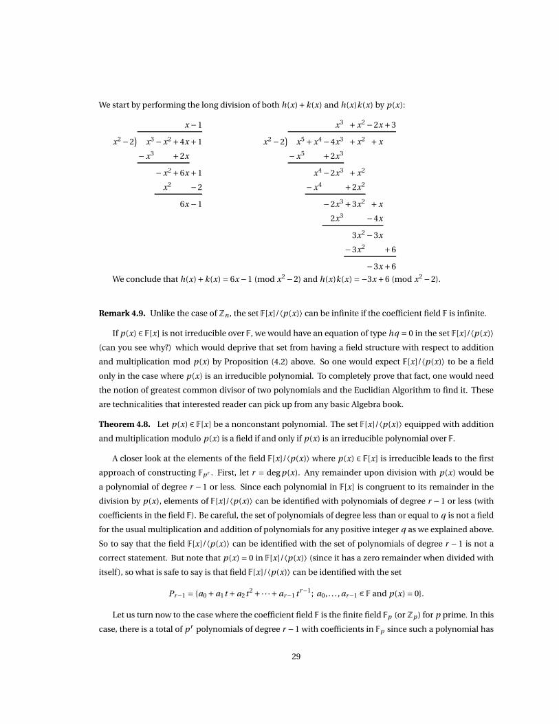
We start by performing the long division of both h(x)+k(x) and h(x)k(x) by p(x):

x −1

x2 −2)

x3 − x2 +4x +1

− x3 +2x

− x2 +6x +1

x2 −2

6x −1

x3 + x2 −2x +3

x2 −2)

x5 + x4 −4x3 + x2 + x

− x5 +2x3

x4 −2x3 + x2

− x4 +2x2

−2x3 +3x2 + x

2x3 −4x

3x2 −3x

−3x2 +6

−3x +6

We conclude that h(x)+k(x) = 6x −1 (mod x2 −2) and h(x)k(x) =−3x +6 (mod x2 −2).

Remark 4.9. Unlike the case of Zn , the set F[x]/⟨p(x)⟩ can be infinite if the coefficient field F is infinite.

If p(x) ∈ F[x] is not irreducible over F, we would have an equation of type hq = 0 in the set F[x]/⟨p(x)⟩(can you see why?) which would deprive that set from having a field structure with respect to addition

and multiplication mod p(x) by Proposition (4.2) above. So one would expect F[x]/⟨p(x)⟩ to be a field

only in the case where p(x) is an irreducible polynomial. To completely prove that fact, one would need

the notion of greatest common divisor of two polynomials and the Euclidian Algorithm to find it. These

are technicalities that interested reader can pick up from any basic Algebra book.

Theorem 4.8. Let p(x) ∈ F[x] be a nonconstant polynomial. The set F[x]/⟨p(x)⟩ equipped with addition

and multiplication modulo p(x) is a field if and only if p(x) is an irreducible polynomial over F.

A closer look at the elements of the field F[x]/⟨p(x)⟩ where p(x) ∈ F[x] is irreducible leads to the first

approach of constructing Fpr . First, let r = deg p(x). Any remainder upon division with p(x) would be

a polynomial of degree r −1 or less. Since each polynomial in F[x] is congruent to its remainder in the

division by p(x), elements of F[x]/⟨p(x)⟩ can be identified with polynomials of degree r −1 or less (with

coefficients in the field F). Be careful, the set of polynomials of degree less than or equal to q is not a field

for the usual multiplication and addition of polynomials for any positive integer q as we explained above.

So to say that the field F[x]/⟨p(x)⟩ can be identified with the set of polynomials of degree r − 1 is not a

correct statement. But note that p(x) = 0 in F[x]/⟨p(x)⟩ (since it has a zero remainder when divided with

itself), so what is safe to say is that field F[x]/⟨p(x)⟩ can be identified with the set

Pr−1 = {a0 +a1t +a2t 2 +·· ·+ar−1t r−1; a0, . . . , ar−1 ∈ F and p(x) = 0}.

Let us turn now to the case where the coefficient field F is the finite field Fp (or Zp ) for p prime. In this

case, there is a total of pr polynomials of degree r −1 with coefficients in Fp since such a polynomial has

29

r coefficients (the degree of the polynomial+1) each of which can take on p values in the field Fp . So the

set Pr−1 above has exactly pr elements.

The following Theorem is a summary of the above discussion and it represents our First attempt at

constructing the Field Fpr . Of course, a complete proof would require checking more details, but at this

point the hope is that the reader finds it somehow reasonable to digest.

Theorem 4.9. Let q(x) ∈ F[x] be monic irreducible polynomial with deg q(x) = r ≥ 1. The field F[x]/⟨q(x)⟩can be identified with polynomials of degree r −1 with coefficients in F together with the condition p(x) =0. Moreover, if F is the finite field Fp (with p prime), then the field F[x]/⟨q(x)⟩ is finite with pr elements.

Example 4.17. Let p(x) = x3 + x +1 considered as an element of F2[x]. We start by proving that p(x) is

irreducible over F2. Suppose not, then there exist a,b,c ∈ Z2 such that (x + a)(x2 + bx + c) = x3 + x + 1.

Consequently,

x3 + x +1 = x3 + (a +b)x2 + (ab +c)x +ac.

Comparing corresponding coefficients on both sides leads to the following equations: a+b = 0, ab+c = 0

and ac = 1 which obviously cannot be satisfied at the same time in the field Z2. Thus, p(x) is irreducible.

Note that another way to check irreducibility of p(x) is to show that it does not have any root in the field

Z2: p(0) = 1 6= 0 and p(1) = 13 + 12 + 1 = 1 6= 0. We conclude that p(x) = x3 + x2 + 1 is irreducible and

so Z2[x]/⟨x3 + x +1⟩ is indeed a field. Let us now look at a description of the elements of this field. By

Theorem 4.9, we know that

Z2[x]/⟨x3 + x +1⟩ ∼={

a0 +a1t +a2t 2; a0, a1, a2 ∈Z2; and t 3 + t +1 = 0}

.

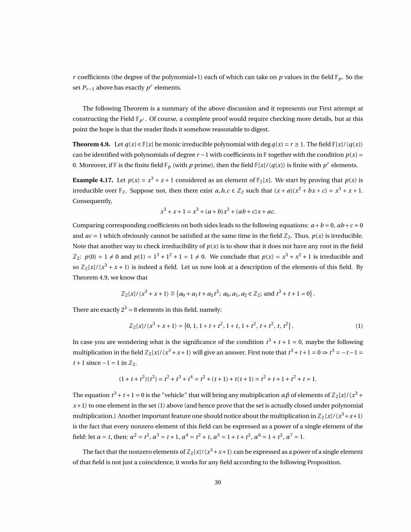
There are exactly 23 = 8 elements in this field, namely:

Z2[x]/⟨x3 + x +1⟩ ={

0, 1, 1+ t + t 2, 1+ t , 1+ t 2, t + t 2, t , t 2}

. (1)

In case you are wondering what is the significance of the condition t 3 + t + 1 = 0, maybe the following

multiplication in the field Z2[x]/⟨x3+x+1⟩ will give an answer. First note that t 3+ t +1 = 0⇒ t 3 =−t −1 =t +1 since −1 = 1 in Z2.

(1+ t + t 2)(t 2) = t 2 + t 3 + t 4 = t 2 + (t +1)+ t(t +1) = t 2 + t +1+ t 2 + t = 1.

The equation t 3+ t +1 = 0 is the "vehicle" that will bring any multiplication αβ of elements of Z2[x]/⟨x3 +x+1⟩ to one element in the set (1) above (and hence prove that the set is actually closed under polynomial

multiplication.) Another important feature one should notice about the multiplication inZ2 [x]/⟨x3+x+1⟩is the fact that every nonzero element of this field can be expressed as a power of a single element of the

field: let α= t , then: α2 = t 2, α3 = t +1, α4 = t 2 + t , α5 = 1+ t + t 2, α6 = 1+ t 2, α7 = 1.

The fact that the nonzero elements ofZ2[x]/⟨x3+x+1⟩ can be expressed as a power of a single element

of that field is not just a coincidence, it works for any field according to the following Proposition.

30

Proposition 4.3. If (F, +, ×) is a finite field, then (F∗,×) is a cyclic group. Here F∗ is, as usual, the field F

from which the zero element is removed.

Proof

Assume that the field F has r elements. Let γ ∈ F∗, and let m = |γ| be the order of γ as an element of the

multiplicative group (F∗,×). As defined above, m is the smallest positive integer satisfying γm = 1 and by

Theorem (4.6), it is at the same time equal to the order of the subgroup Pγ = {γi ; i ∈N} of (F∗,×) generated

by γ. This means in particular that γ is a root of the polynomial xm − 1 of F[x]. By Lagrange Theorem

(Theorem 4.5), we know that m is a divisor of r −1 ( since |F∗| = r −1), so γr−1 = γkm =(

γm)k = 1k = 1

and γ is actually a root of the polynomial xr−1 −1 = 0. To prove that (F∗,×) is cyclic, it is enough to find

a nonzero element with order equal to r − 1. Suppose such an element does not exist and let k be the

largest order of a nonzero element of F. Then k < r −1 and every nonzero element of F is a root of the

polynomial xk −1 = 0. But the equation xk −1 = 0 has at most k roots in the field F which contradicts the

fact that all the r −1 elements of F∗ are roots. We conclude that an element α of order r −1 exists and that

F∗ = {1, α, α2, . . . ,αr−2} is a cyclic group.

Definition 4.10. A primitive element of a finite field (F, +, ×) is any generator of the cyclic group (F∗, ×).

In other words, if |F| = r , then α ∈ F∗ is primitive if F∗ = {1, α, α2, . . . , αr−2}.

Example 4.18. In Example 4.17 above, α= t is a primitive element of the field Z2[x]/⟨x3 + x +1⟩.

Now for the second approach to construct Fpr . Recall that the field Fp containing p elements is noth-

ing but a copy of the field Zp of all integers modulo p.

Consider the set Zpr = Zp ×Zp ×·· ·×Zp

︸ ︷︷ ︸

r

of all r -tuples (a0, a1, . . . , ar−1) where ai ∈ Zp for all i . Our

second construction of the finite field Fpr is done by "identifying" Fpr with Zpr after defining suitable ad-

dition and multiplication of r -tuples.

We define an addition on Zrp the natural way:

(a0, a1, . . . , ar−1)+ (b0,b1, . . . ,br−1) = (a0 +b0, a1 +b1, . . . , ar−1 +br−1)

where ai +bi represents the addition mod p in Zp .

The multiplication on Zrp will probably appear to you as very "unnatural". We start by fixing an irre-

ducible and monic polynomial of degree r in Zp [x]:

M(t) = t r +mr−1t r−1 +·· ·+m1t +m0.

Each r -tuple (a0, a1, . . . , ar−1) ∈Zpr is identified with the polynomial p(t)= ar−1t r−1+·· ·+a1t+a0 ∈Zp [t ]

of degree less than or equal to r −1 with coefficients in the field Zp .

31

To define the multiplication of two r -tuples (a0, a1, . . . , ar−1), (b0,b1, . . . ,br−1) of Zpr , we start by writ-

ing the corresponding polynomials in Zp [t ]:

p(t)= ar−1t r−1 +·· ·+a1t +a0, q(t)= br−1t r−1 +·· ·+b1t +b0,

then we multiply the two polynomials together in the usual way by regrouping terms in t 0, t , t 2,..., t 2(r−1):

p(t)q(t)= ar−1br−1t 2(r−1) +·· ·+ (a0b1 +a1b0)t +a0b0

which in turns is congruent to its remainder R(t) modulo M(t) as an element of F[t ]/⟨M(t)⟩. Since the

remainder is of degree less than or equal to r −1, it can be written under the form R(t) =αr−1t r−1 +·· ·+α1t +α0 where αi ∈ F for all i . Now define the multiplication of the two r -tuples (a0, a1, . . . , ar−1) and

(b0,b1, . . . ,br−1) as being the r -tuple consisting of the coefficients of R(t):

(a0, a1, . . . , ar−1)× (b0,b1, . . . ,br−1) = (α0,α1, . . . ,αr−1).

Remark 4.10. The key feature in this second approach is the fact that it allows us to look at the r -tuples

of Fpr as polynomials. More importantly, the multiplication on Fp

r defined above with respect to the

polynomial M(t) produces the same results when the r -tuples are identified with polynomials of degree

less than or equal to r −1 and we multiply them modulo M(t) in Fp [t ]. Formally, we say that the two fields

Fpr and Fpr are isomorphic (one is a copy of the other). This means in particular that the set Zp

r equipped

with the above addition and multiplication with respect to a monic irreducible polynomial M(t) is indeed

a field.

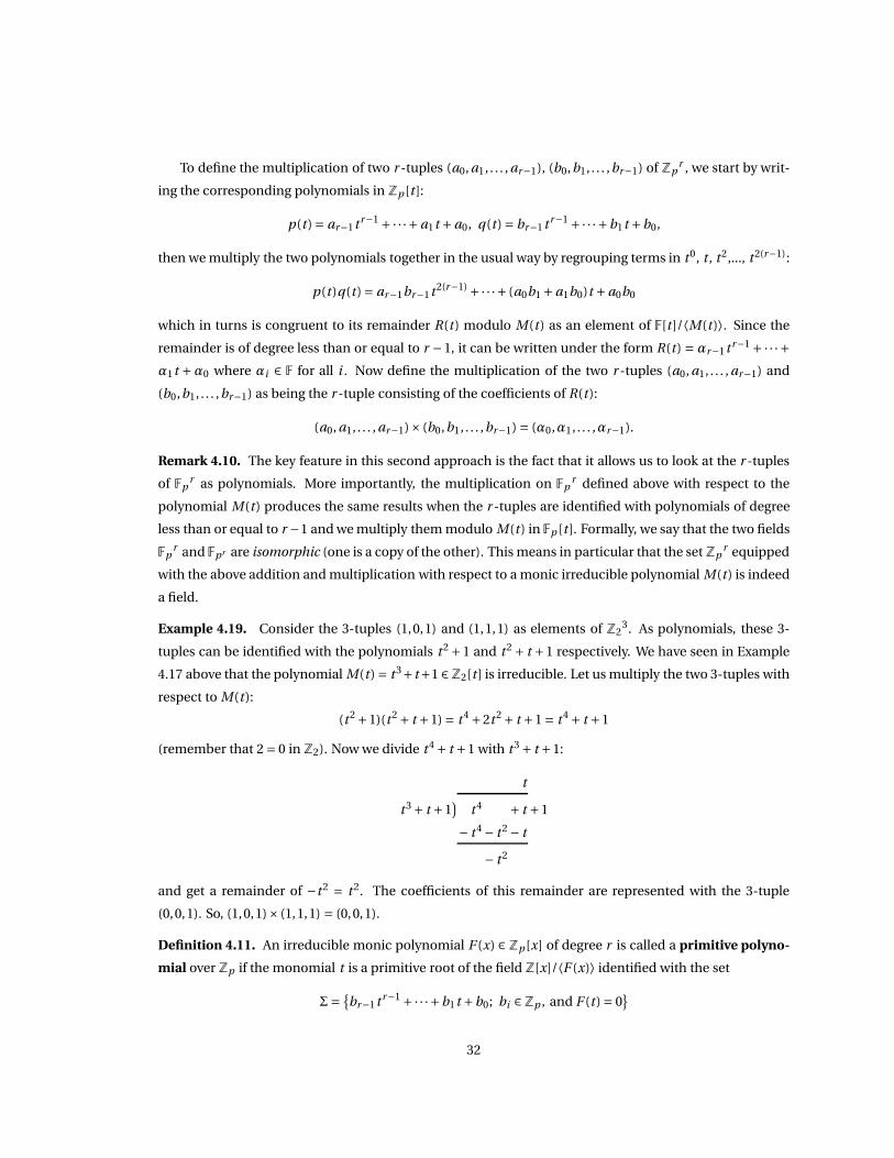
Example 4.19. Consider the 3-tuples (1,0,1) and (1,1,1) as elements of Z23. As polynomials, these 3-

tuples can be identified with the polynomials t 2 +1 and t 2 + t +1 respectively. We have seen in Example

4.17 above that the polynomial M(t) = t 3+t+1 ∈Z2[t ] is irreducible. Let us multiply the two 3-tuples with

respect to M(t):

(t 2 +1)(t 2 + t +1) = t 4 +2t 2 + t +1 = t 4 + t +1

(remember that 2 = 0 in Z2). Now we divide t 4 + t +1 with t 3 + t +1:

t

t 3 + t +1)

t 4 + t +1

− t 4 − t 2 − t

− t 2

and get a remainder of −t 2 = t 2. The coefficients of this remainder are represented with the 3-tuple

(0,0,1). So, (1,0,1)× (1,1,1) = (0,0,1).

Definition 4.11. An irreducible monic polynomial F (x) ∈ Zp [x] of degree r is called a primitive polyno-

mial over Zp if the monomial t is a primitive root of the field Z[x]/⟨F (x)⟩ identified with the set

Σ={

br−1t r−1 +·· ·+b1t +b0; bi ∈Zp , and F (t)= 0}

32

Example 4.20. In Example 4.17 above, the polynomial P (x) = x3 + x + 1 ∈ Z2[x] is primitive since it is

irreducible and t is a primitive element of the field Z2[x]/⟨x3 + x +1⟩.

Example 4.21. The polynomial x6 + x3 +1 ∈ Z2[x] is irreducible since it has no roots in Z2. On the other

hand, the equation t 6 + t 3 +1 = 0 in the field Z2[x]/⟨x3 + x +1⟩ is equivalent to t 6 =−t 3 −1 = t 3 +1. This

gives the following powers of the monomial t :

t 7 = t 4 + t , t 8 = t 5 + t 2, t 9 = t 6 + t 3 = t 3 +1+ t 3 = 2t 3 +1 = 1.

The fact that t 9 = 1 and that the multiplicative group of F[x]/⟨x3 +x+1⟩ is of order 26 −1 = 63 imply that t

is not a generator of that group. So the polynomial x6 + x3 +1 of Z2[x] is not primitive.

Remark 4.11. If α is a primitive root of a finite field F with |F| = r , the proof of Proposition 4.3 shows in

particular that α is a root of the polynomial Q(x) = xr−1 −1 and that r −1 is the smallest integer m such

that α is a root of xm −1. It can also be shown that the polynomial F (x) is a primitive polynomial if the

smallest positive integer n such that F (x) divides xn −1 is indeed n = r −1.

The following Theorem proves that there is enough supply of primitive polynomials of any chosen

degree.

Theorem 4.10. For any prime integer p and any positive integer n, there exists a primitive polynomial of

degree n over the field Zp .

4.5 The Trace

Definition 4.12. A map f : Fpr → Fp is called linear if it satisfies the two conditions:

1. f (~u+~v) = f (~u)+ f (~v) for all r -tuples ~u, ~v in Fpr

2. f (α~u) =α f (~u) for all ~u ∈ Fpr and α ∈ Fp

Example 4.22. Let F (x) be an irreducible polynomial of degree r in Fp [x] and identify the field Fpr ∼=

Fp [x]/⟨F (x)⟩ as usual with the set of polynomials of degree r −1 or less together with the identity F (t)= 0.

Consider the map θ : Fpr → Fp , called the Trace function, defined as follows:

θ(

br−1t r−1 +·· ·+b1t +b0

)

= br−1.

If ~u = br−1t r−1 +·· ·+b1t +b0, ~v = cr−1t r−1 +·· ·+c1t +c0 ∈ Fpr and α∈ Fp , then

• θ (~u +~v) = θ(

(br−1 +cr−1)t r−1 +·· ·+ (b1 +c1)t + (b0 +c0))

= br−1 +cr−1 = θ (~u)+θ (~v).

• θ (α~u) = θ(

αbr−1t r−1 +·· ·+αb1t +αb0

)

=αbr−1 =αθ (~u).

33

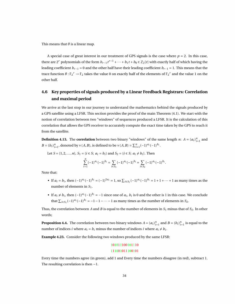
This means that θ is a linear map.

A special case of great interest in our treatment of GPS signals is the case where p = 2. In this case,

there are 2r polynomials of the form br−1t r−1 +·· ·+b1t +b0 ∈Z2[t ] with exactly half of which having the

leading coefficient br−1 = 0 and the other half have their leading coefficient br−1 = 1. This means that the

trace function θ : F2r → F2 takes the value 0 on exactly half of the elements of F2

r and the value 1 on the

other half.

4.6 Key properties of signals produced by a Linear Feedback Registrars: Correlation

and maximal period

We arrive at the last stop in our journey to understand the mathematics behind the signals produced by

a GPS satellite using a LFSR. This section provides the proof of the main Theorem (4.1). We start with the

notion of correlation between two "windows" of sequences produced a LFSR. It is the calculation of this

correlation that allows the GPS receiver to accurately compute the exact time taken by the GPS to reach it

from the satellite.

Definition 4.13. The correlation between two binary "windows" of the same length n: A = (ai )ni=1

and

B = (bi )ni=1

, denoted by ν(A,B), is defined to be ν(A,B) =∑n

i=1(−1)ai (−1)bi .

Let S = {1,2, . . . ,n}, S1 = {i ∈ S; ai = bi } and S2 = {i ∈ S; ai 6= bi }. Then

n∑

i=1

(−1)ai (−1)bi =∑

i∈S1

(−1)ai (−1)bi +∑

i∈S2

(−1)ai (−1)bi .

Note that:

• If ai = bi , then (−1)ai (−1)bi = (−1)2ai = 1, so∑

i∈S1(−1)ai (−1)bi = 1+1+·· · +1 as many times as the

number of elements in S1.

• If ai 6= bi , then (−1)ai (−1)bi =−1 since one of ai , bi is 0 and the other is 1 in this case. We conclude

that∑

i∈S1(−1)ai (−1)bi =−1−1−·· · −1 as many times as the number of elements in S2.

Thus, the correlation between A and B is equal to the number of elements in S1 minus that of S2. In other

words;

Proposition 4.4. The correlation between two binary windows A = (ai )ni=1

and B = (bi )ni=1

is equal to the

number of indices i where ai = bi minus the number of indices i where ai 6= bi .

Example 4.23. Consider the following two windows produced by the same LFSR:

101011100101110

111001011100101

Every time the numbers agree (in green), add 1 and Every time the numbers disagree (in red), subtract 1.

The resulting correlation is then −1.

34

Let us now revisit the LFSR as shown in Figure 1 above. Fix a primitive polynomial of degree r over Z2:

P (x) = xr +cr−1xr−1 +·· ·+c1x +c0

whose existence is guaranteed by Theorem 4.10 above. For the coefficient vector of the LFSR, choose

the vector c = (cr−1, · · · , c1, c0) whose components are the coefficients of P (x). The choice of the initial

conditions (the secret code of the LSFR) is a bit more complicated and uses the Trace function θ : Fpr → Fp

defined in Example 4.22 above. We follow the following steps:

1. Start by choosing any nonzero polynomial ǫ(t) of degree r −1 in Z2[x]/⟨P (x)⟩ identified with the set

Σ={

br−1t r−1 +·· ·+b1t +b0; bi ∈Zp and P (t) = 0}

:

ǫ(t) = ǫr−1t r−1 +·· ·+ǫ1t +ǫ0, ǫi ∈Z2 for all i = r −1, . . . ,0.

2. Define a0 = θ(ǫ) = ǫr−1.

3. Next, we compute tǫ(t) as an element of Z2[x]/⟨P (x)⟩. Remember that the equation P (t) = 0 trans-

lates to t r = cr−1t r−1 +·· ·+c1t +c0 since −ci = ci in the field Z2.

tǫ(t) = t(

ǫr−1t r−1 +·· ·+ǫ1t +ǫ0

)

= ǫr−1t r +ǫr−2t r−1 · · ·+ǫ1t 2 +ǫ0t

= ǫr−1

(

cr−1t r−1 +·· ·+c1t +c0

)

+ǫr−2t r−1 · · ·+ǫ1t 2 +ǫ0t

= (ǫr−1cr−1 +ǫr−2) t r−1 +·· ·+ (ǫr−1c1 +ǫ0) t +ǫr−1c0

4. Define a1 = θ(tǫ(t)) = ǫr−1cr−1 +ǫr−2

5. To define a2, we compute first t 2ǫ(t) as a polynomial of degree r −1 in t (always using the identity

P (t)= 0) and then we define a2 as the trace of that polynomial: a2 = θ(t 2ǫ(t))

6. In general, ai = θ(t i ǫ(t)) for all i ∈ {0,1, . . . ,r −1}.

7. We take (a0, a1, ..., ar−1) to be the initial window of the LFSR.

But what is the big deal? why do we need P (x) to be primitive and why this complicated way of choos-

ing the initial window? Be patient, you have gone a long way so far and the answers will follow shortly.

Note that:

θ(t r ǫ) = θ(cr−1 t r−1ǫ+·· ·+c1tǫ+c0ǫ) (since t r = cr−1t r−1 ++·· ·+c1t +c0)

= cr−1θ(t r−1ǫ)+·· ·+c1θ(tǫ)+c0θ(ǫ) (by the linearity of the trace map θ)

= cr−1ar−1 +·· ·+c1a1 +c0a0 (by our definition of the initial conditions a0, . . . , ar−1)

35

Look closely at the last expression. Isn’t that the way the LFSR computes its next term ar ? We conclude

that θ(t r ǫ) = ar . In fact, it is not hard to show that any term in the sequence produced by a LFSR can be

obtained this way. More specifically,

ak = θ(t kǫ), k = 0,1,2, . . . (1)

The proof is left to the reader.

We are now ready to prove Theorem 4.1.

Proof of Theorem 4.1. With the above choice of the coefficients (as coefficients of a primitive polynomial)

and the secret code, we show that the minimal period of a sequence produced by a LFSR with r registers is

precisely N = 2r −1. We already know (see Remark 4.1) that the sequence is periodic and that the maximal

length of its minimal period is 2r . Assume that T is the minimal period of the sequence. Since P (x) is

chosen to be a primitive polynomial, t is a generator of the multiplicative group of the field Z2[x]/⟨P (x)⟩which contains N = 2r −1 elements and therefore t N = 1. Moreover, for any n ∈N, we have

an+N = θ(t n+N ǫ) = θ(t N t nǫ) = θ(t nǫ) = an .

This shows in particular that N = 2r −1 is a period of the sequence and by the minimality of T , we have

that T ≤ N . On the other hand, given k ∈ N, the equation ak+T = ak translates to θ(t k+T ǫ) = θ(t kǫ) or

equivalently to

θ(t kǫ(t T −1)) = 0 (2)

by the linearity of θ. Assume (t T −1) 6= 0, then ǫ(t T −1) 6= 0 as a product of two nonzero elements of the

field Z2[x]/⟨P (x)⟩. But remember that P (x) was chosen to be minimal for a reason: any nonzero element

of Z2[x]/⟨P (x)⟩ is a power of t , in particular ǫ(t T − 1) = t n for some n ∈{

0,1,2, . . . ,2r −2}

and therefore

t kǫ(t T −1) = t k+n . The elements t kǫ(t T −1) are then just permutations of the elements of multiplicative

group F∗2r ={

1, t , t 2, . . . , t N−1}

. Equation (2) implies that the trace function θ takes the value zero every-

where on F∗2r which is absurd. Therefore t T −1 = 0 or equivalently t T = 1. By definition of the order of

t as element of the multiplicative group of the field Z2[x]/⟨P (x)⟩, N = 2r −1 is the smallest positive inte-

ger satisfying t N = 1. Since T ≤ N and t T = 1, we conclude that T = N and so the minimal period of the

sequence an is indeed N = 2r −1.

We can actually say more about the sequence produced by a LFSR as constructed above.

Theorem 4.11. Consider the binary sequence produced by a LFSR with r registers constructed using the

coefficients of a primitive polynomial and secret code produced by the Trace function as above. Let W1 =(an , an+1, . . . , an+N−1) and W2 = (am , am+1, . . . , am+N−1) be two windows (with m > n) of the sequence of

length equal to the minimal period N = 2r −1 of the sequence. Then the correlation ν between W1 and

36

W2 is given by:

ν={

−1 if m −n is not a multiple of N

N if m −n is a multiple of N

Proof

We use the definition of the windows correlation,

ν =N−1∑

k=0

(−1)an+k (−1)am+k

=N−1∑

k=0

(−1)θ(t n+k ǫ)(−1)θ(t m+k ǫ) (By relation (1) above)

=N−1∑

k=0

(−1)θ(t n+k ǫ)+θ(t m+kǫ)

=N−1∑

k=0

(−1)θ(

t n+k ǫ+t m+kǫ)

(By the linearity of the trace function)

=N−1∑

k=0

(−1)θ(

t n+k ǫ(1+t m−n))

.

If m−n = ρN is a multiple of N , then t m−n =(

t N)ρ = 1 since t N = 1 (remember that t is the generator of a

group of order N ), so 1+t m−n = 2 = 0 and (−1)θ(

t n+kǫ(1+t m−n))

= 1 for all k in this case. This implies that the

correlation is ν = 1+1+·· · +1︸ ︷︷ ︸

N

= N . Assume next that m −n is not a multiple of N , then the polynomial

1+ t m−n is nonzero and therefore ǫ(1+ t m−n ) is also nonzero as the product of two nonzero elements of

the field Z2[x]/⟨P (x)⟩. As in the proof of Theorem 4.1, the fact that P (x) is chosen to be primitive comes

in very handy now:

ǫ(

1+ t m−n)

6= 0⇒ ǫ(

1+ t m−n)

= t j for some j ∈ {0,1,2, . . . , N −1}.

As k takes all values in the set {0,1, . . . , N − 1}, the elements t n+kǫ(1+ t m−n ) = t j+n+k are just permuta-

tions of the elements of F∗2r = {1, t , t 2, . . . , t N−1}. As seen above, the trace function takes he value 0 on

exactly half of the elements of the set F2r and the value 1 on the other half. This implies in particular that∑

αi∈F2r (−1)θ(αi ) = 0. Now, since (−1)θ(0) = 1, the last sum in the above expression of ν can be written as

N−1∑

k=0

(−1)θ(

t n+k ǫ(1+t m−n))

=∑

αi∈F2r

(−1)θ(αi )

︸ ︷︷ ︸

0

−(−1)θ(0) =−1.

This proves that the correlation between the two window is −1 in this case

This is indeed an amazing fact: Take any two windows of the same length 2r −1 (length of a minimal

period) in a sequence produced by a LFSR, then you are that the number of terms which disagree is always

one more than the number of terms which agree (provided, as in the Theorem, that m−n is not a multiple

of N = 2r −1)

37

4.7 How is the Shifting of signals would tell the time?

Each satellite transmits a pseudo random code (PRN) in the form of a sequence of packages of "chips"

which the receiver can decode, convert into a binary sequence and compare with the pseudo random

codes stored in its memory. As explained earlier, the two codes will not coincide because of the run-

time of the signal from the satellite. The GPS receiver shifts its signal by one unit and compares with the

captured signal by calculating the correlation between the two windows. This process is repeated until

a correlation zero is attained and hence perfect synchronization between the two signals. The receiver

records the number n of "shifts" needed to acheive that perfect synchronization.

The LFSR used to produce the satellite code has r = 10 cells, producing a sequence of minimal period of

210−1 = 1023 bits by the above discussion. Practically, this means that each "window" of the satellite PNR

is formed by 1023 chips. The satellite PNR is transmitted at a speed of 1.023 MHz or 1023000 cycles (or

windows) per second. This means that every window of minimal period is repeated every 0.001 second

(or 1000 microseconds). At the speed of 299,792,458 meters per second (speed of light), 0.001 second cor-

respond to a distance of 299.792458 km. Dividing this distance with the minimal period of the sequence

(1023) would give a distance of 0.293052256 km per chip. The departure time from the satellite of the start

of the window is encrypted in the code and hence is known by the receiver. The number n of shifts is then

multiplied by 0.293052256 and the result is divided by the speed of light. The answer that we get is the

time gap between the departure of the window from the satellite (according to the satellite clock) and the

arrival time to the reception (according to the receiver clock).

38