Embed Size (px)
DESCRIPTION
How types of market differ, and why it matters. Michael Joffe Imperial College London PKSG, Cambridge, November 2011. Structure of the talk. the current discourse: the market vs. the state market failure real-economy competition between firms: cost-tethered markets - PowerPoint PPT Presentation
Citation preview

How types of market differ, and why it matters
Michael Joffe Imperial College London
PKSG, Cambridge, November 2011
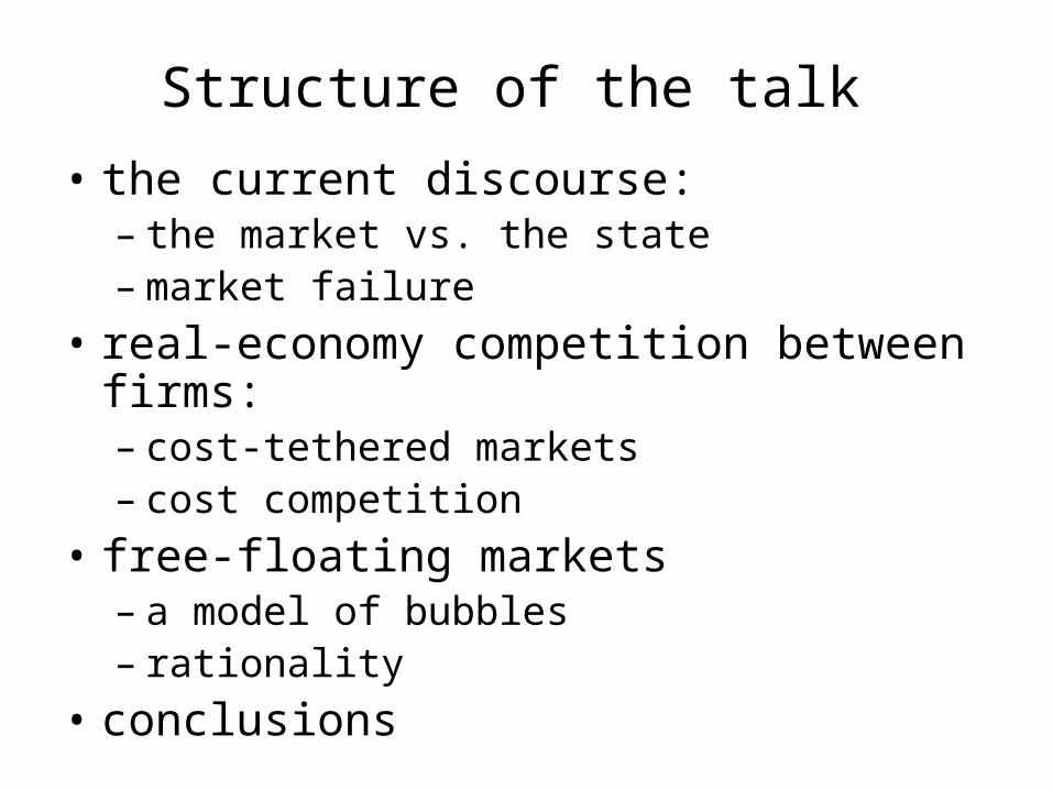
Structure of the talk
• the current discourse: – the market vs. the state – market failure
• real-economy competition between firms: – cost-tethered markets – cost competition
• free-floating markets – a model of bubbles – rationality
• conclusions
Structure of the talk
• the current discourse: – the market vs. the state – market failure
• real-economy competition between firms: – cost-tethered markets – cost competition
• free-floating markets – a model of bubbles – rationality
• conclusions
The current discourse I • a large part of economic theory concerns the
properties of “the market” • central to this is, under certain assumptions,
“the” market has a particular set of properties: convergence towards a stable equilibrium (and under certain conditions, Pareto optimality)
• observation: not all economic phenomena can readily be explained using this framework – most recently bubbles/crises; but also the specific property of capitalism, that it grows – exogenous technical change, or smithian growth
The current discourse II • criticisms typically focus on the assumptions
being unrealistic, or on market failure of various types, e.g. monopoly power, missing or incomplete markets, externalities, public goods or information asymmetry – “failure” => the market does not work as the
theory would predict (i.e. the theory itself is OK)
• more broadly, the discourse is one of “the” market versus the state – with a political dimension, in which theory is evaluated largely in the light of one’s political values
Types of market I • the term “types of market” has a number of
possible meanings: • place: local, national, international • time: very short, short, long, very long period • the ideal types of textbook theory: perfect
competition, monopoly, duopoly, oligopoly, monopolistic competition, monopsony
• different types of goods: inferior, luxury, Geffen, positional goods; winner-take-all markets
Types of market II • various arbitrary divisions, e.g.
– physical, internet, labour, intermediate goods, stock market, ad hoc auctions, illegal markets, ...
– financial markets, currency markets, futures markets, the money market (lending/borrowing)
– consumer, industrial, commodity and capital markets
• I argue: different types of market have radically different dynamic behaviour, for reasons that can be readily understood, and this can be modelled

Structure of the talk
• the current discourse: – the market vs. the state – market failure
• real-economy competition between firms: – cost-tethered markets – cost competition
• free-floating markets – a model of bubbles – rationality
• conclusions
Structure of the talk
• the current discourse: – the market vs. the state – market failure
• real-economy competition between firms: – cost-tethered markets – cost competition
• free-floating markets – a model of bubbles – rationality
• conclusions

Real-economy competition between firms I
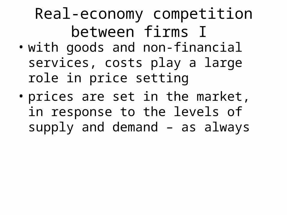
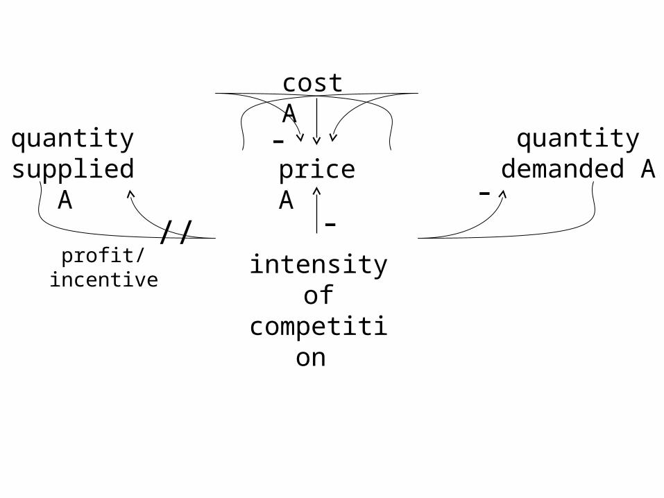
• with goods and non-financial services, costs play a large role in price setting
• prices are set in the market, in response to the levels of supply and demand – as always
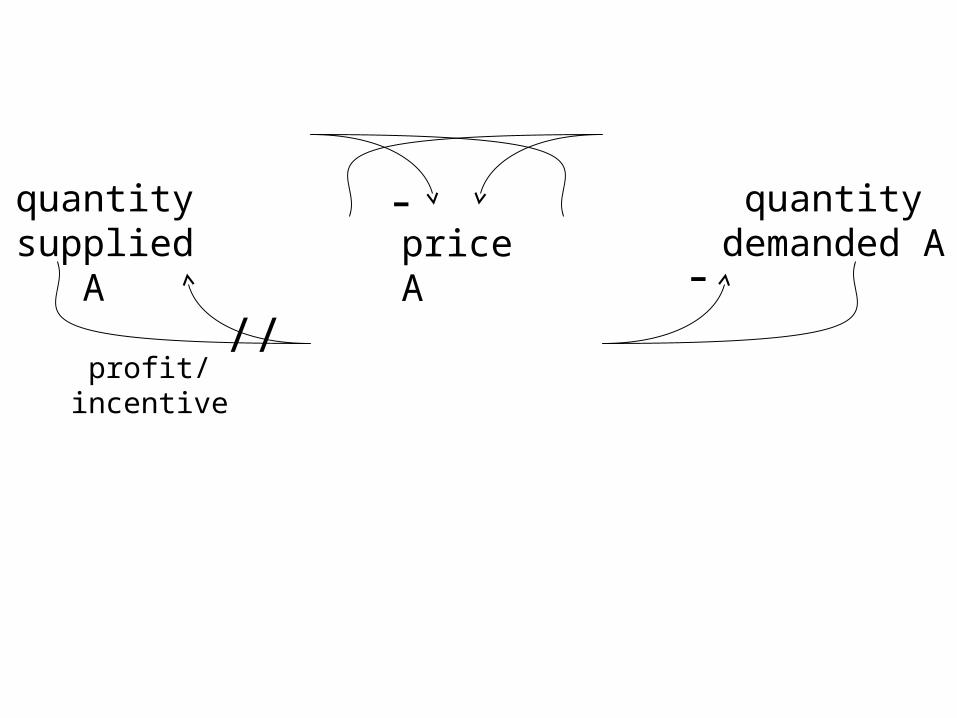
price A quantity
demanded A-quantity
supplied A -
//profit/incentive
Real-economy competition between firms I
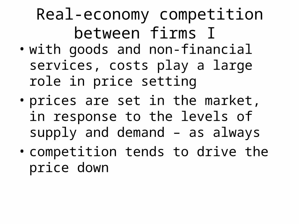
• with goods and non-financial services, costs play a large role in price setting
• prices are set in the market, in response to the levels of supply and demand – as always
Real-economy competition between firms I
• with goods and non-financial services, costs play a large role in price setting
• prices are set in the market, in response to the levels of supply and demand – as always
• competition tends to drive the price down

price A quantity
demanded A-quantity
supplied A -
//profit/incentive
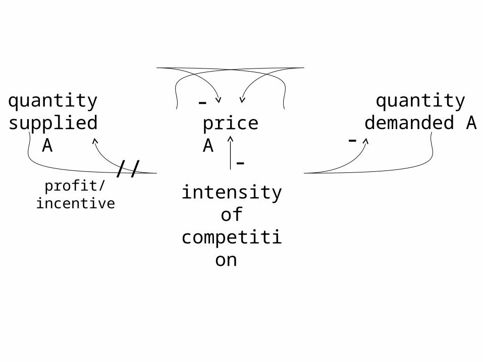
price A quantity
demanded A-
intensity of competition
quantity supplied A
--
//profit/incentive

Real-economy competition between firms I
• with goods and non-financial services, costs play a large role in price setting
• prices are set in the market, in response to the levels of supply and demand – as always
• competition tends to drive the price down
Real-economy competition between firms I
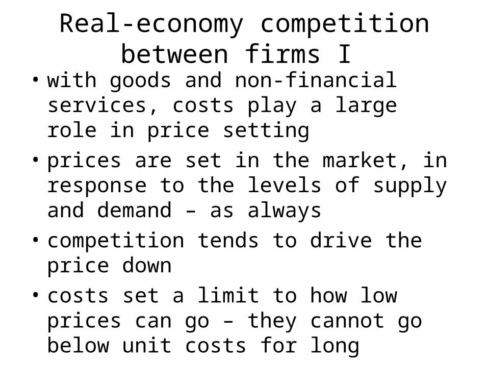
• with goods and non-financial services, costs play a large role in price setting
• prices are set in the market, in response to the levels of supply and demand – as always
• competition tends to drive the price down • costs set a limit to how low prices can go –
they cannot go below unit costs for long

price A quantity
demanded A-
intensity of competition
quantity supplied A
--
//profit/incentive
price A quantity
demanded A-
intensity of competition
quantity supplied A
cost A
--
//profit/incentive
Real-economy competition between firms I • with goods and non-financial services, costs
play a large role in price setting • prices are set in the market, in response to the
levels of supply and demand – as always • competition tends to drive the price down • costs set a limit to how low prices can go –
they cannot go below unit costs for long
Real-economy competition between firms I • with goods and non-financial services, costs
play a large role in price setting • prices are set in the market, in response to the
levels of supply and demand – as always • competition tends to drive the price down • costs set a limit to how low prices can go –
they cannot go below unit costs for long • the result is, prices tend to end up just above
unit costs – the difference is the mark-up • I call this cost tethering
– it is not rigid: the mark-up is variable

price A quantity
demanded A-
intensity of competition
quantity supplied A
cost A
--
//profit/incentive
price A quantity
demanded A-
intensity of competition
quantity supplied A
cost A
--
//profit/incentive
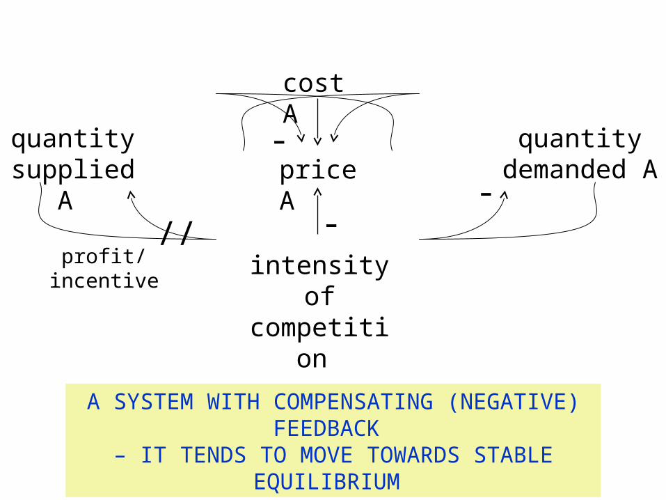
A SYSTEM WITH COMPENSATING (NEGATIVE) FEEDBACK – IT TENDS TO MOVE TOWARDS STABLE EQUILIBRIUM
price A quantity
demanded A-
intensity of competition
quantity supplied A
cost A
--
//profit/incentive
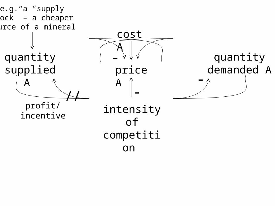
e.g. a “supply shock” – a cheaper source of a mineral
price A quantity
demanded A-
intensity of competition
quantity supplied A
cost A
--
//profit/incentive
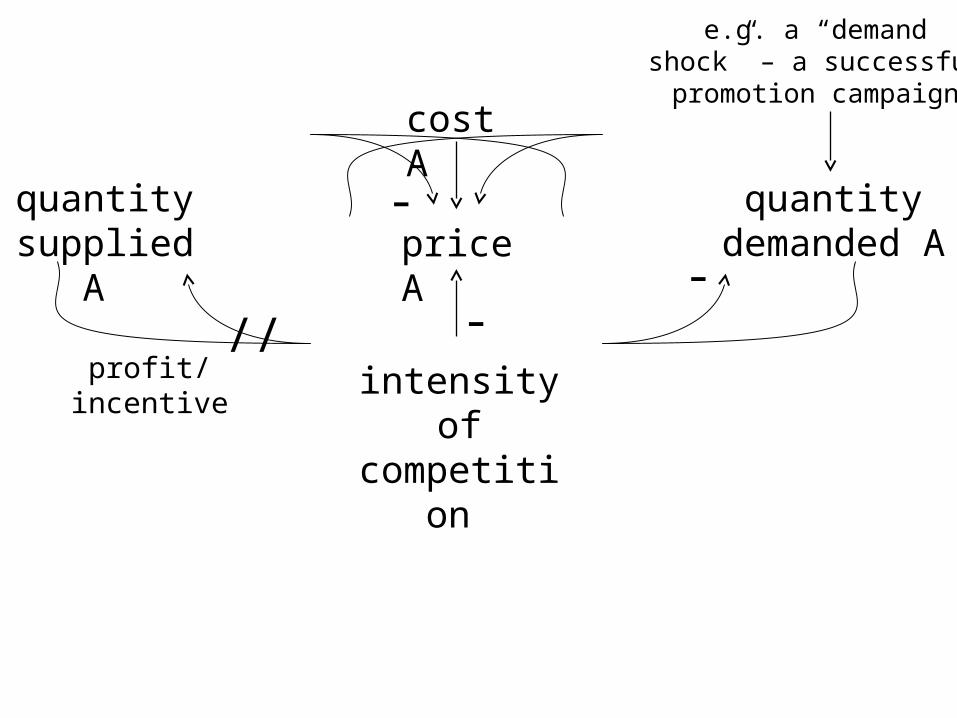
e.g. a “demand shock” – a successful promotion campaign
price A quantity
demanded A-
intensity of competition
quantity supplied A
cost A
--
//profit/incentive
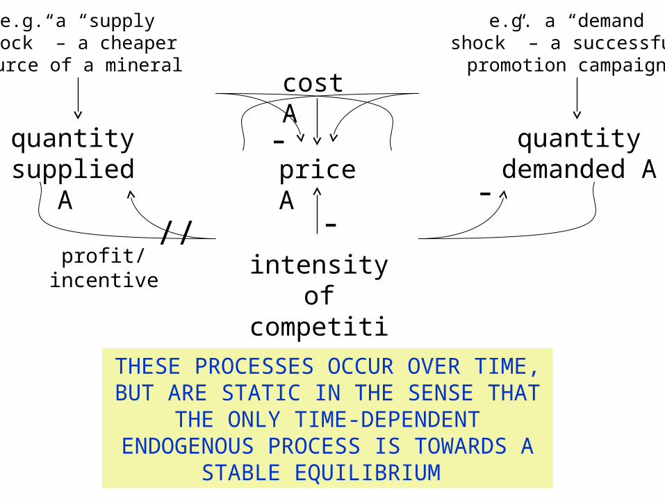
e.g. a “supply shock” – a cheaper source of a mineral
THESE PROCESSES OCCUR OVER TIME, BUT ARE STATIC IN THE SENSE THAT THE ONLY TIME-
DEPENDENT ENDOGENOUS PROCESS IS TOWARDS A STABLE EQUILIBRIUM
e.g. a “demand shock” – a successful promotion campaign

price A quantity
demanded A-
intensity of competition
quantity supplied A
cost A
--
//profit/incentive
price A quantity
demanded A-
intensity of competition
quantity supplied A
cost A
cost B
price B -
--
--
quantity supplied B
quantity demanded B
\\
//profit/incentive
profit/incentive
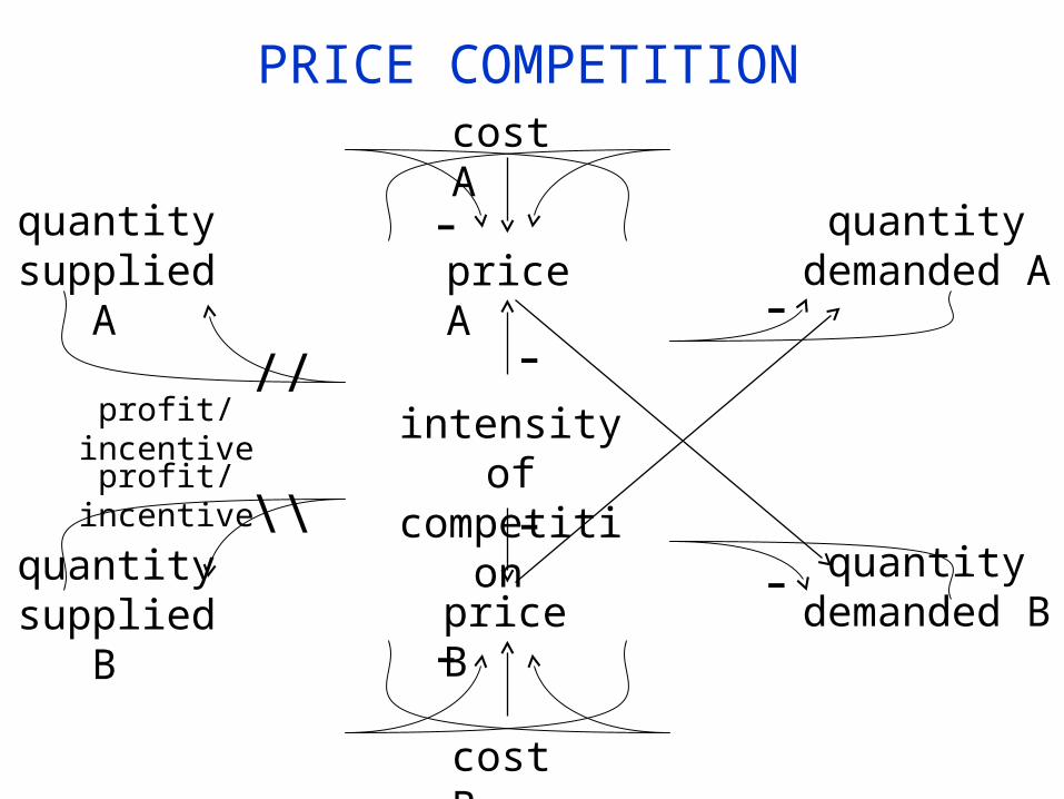
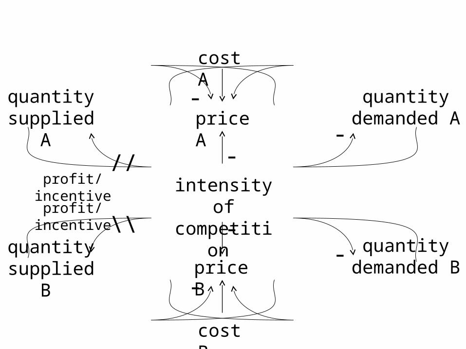
price A quantity
demanded A-
intensity of competition
PRICE COMPETITION
quantity supplied A
cost A
cost B
price B -
--
--
quantity supplied B
quantity demanded B
\\
//profit/incentive
profit/incentive
Real-economy competition between firms II
• so far, I have assumed costs as given – as is conventional in mainstream theory
• what happens if costs can be reduced?
Real-economy competition between firms II
• so far, I have assumed costs as given – as is conventional in mainstream theory
• what happens if costs can be reduced? • this would necessarily be on a longer timescale,
via investment
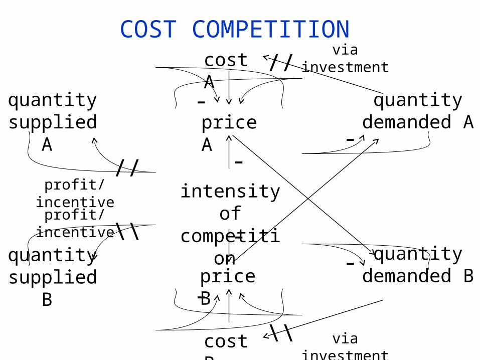
price A quantity
demanded A-
intensity of competition
COST COMPETITION
quantity supplied A
cost A
cost B
price B -
--
--
quantity supplied B
quantity demanded B
\\profit/incentive
profit/incentive//
//via investment
\\ via investment

The standard market equilibrium model
price
quantity
P1
Q1
D
S
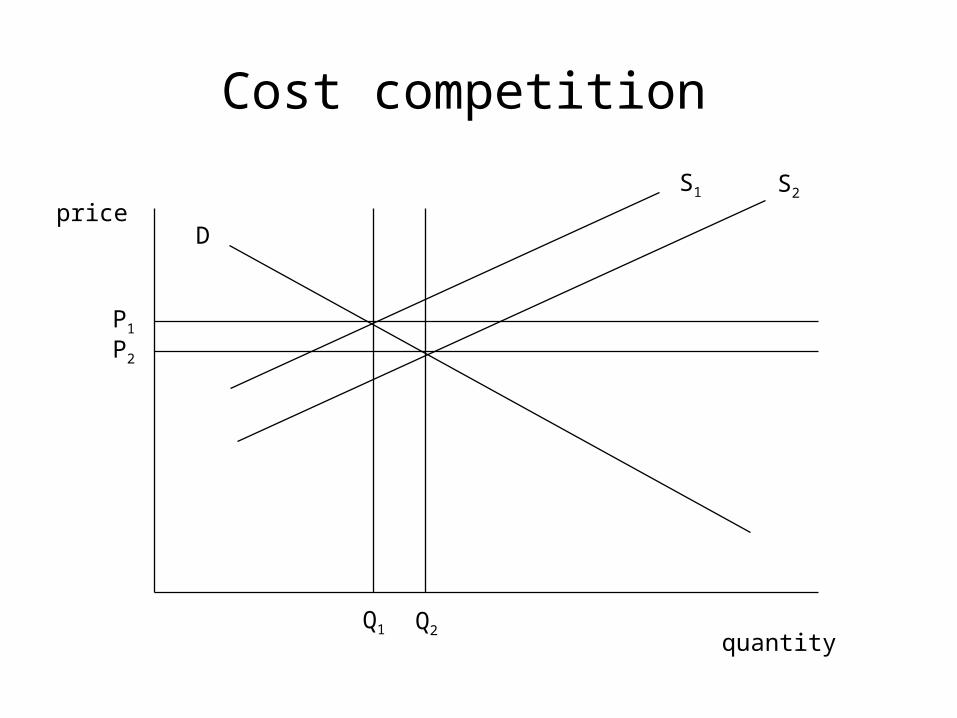
Cost competition
price
quantity
P1
P2
Q2Q1
D
S1 S2
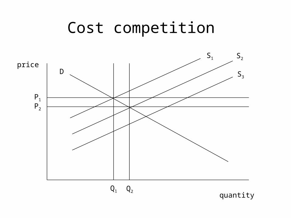
Cost competition
price
quantity
P1
P2
Q2Q1
D
S1 S2
S3
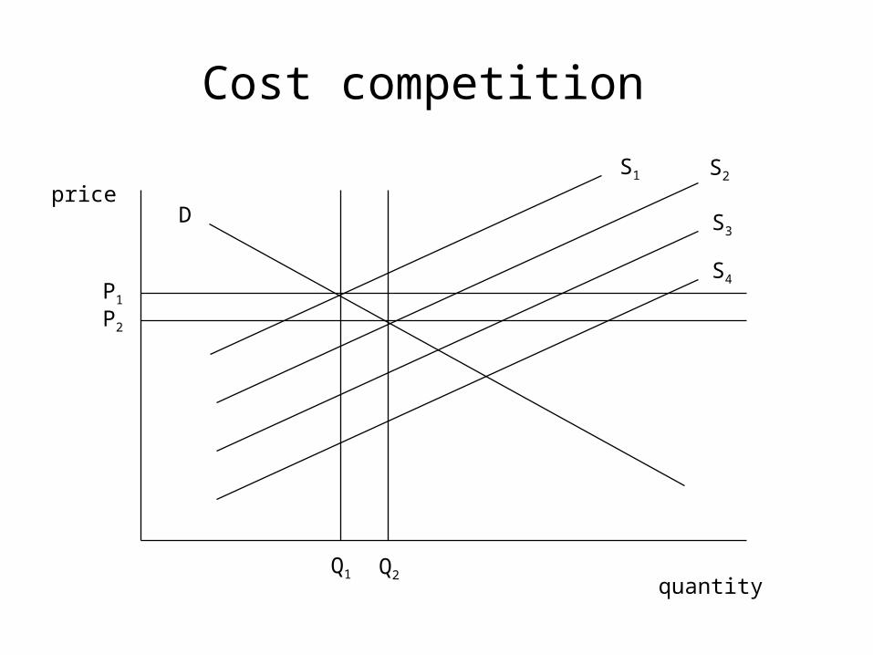
Cost competition
price
quantity
P1
P2
Q2Q1
D
S1 S2
S3
S4
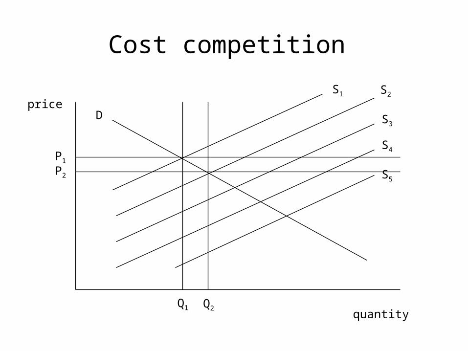
Cost competition
price
quantity
P1
P2
Q2Q1
D
S1 S2
S3
S4
S5
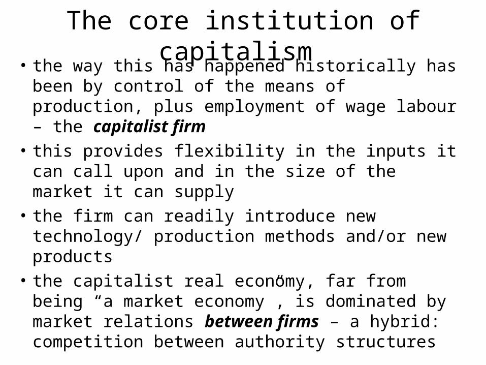
The core institution of capitalism • the way this has happened historically has been
by control of the means of production, plus employment of wage labour – the capitalist firm
• this provides flexibility in the inputs it can call upon and in the size of the market it can supply
• the firm can readily introduce new technology/ production methods and/or new products
• the capitalist real economy, far from being “a market economy”, is dominated by market relations between firms – a hybrid: competition between authority structures
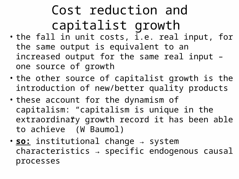
Cost reduction and capitalist growth
• the fall in unit costs, i.e. real input, for the same output is equivalent to an increased output for the same real input – one source of growth
• the other source of capitalist growth is the introduction of new/better quality products
• these account for the dynamism of capitalism: “capitalism is unique in the extraordinary growth record it has been able to achieve” (W Baumol)
• so: institutional change → system characteristics → specific endogenous causal processes
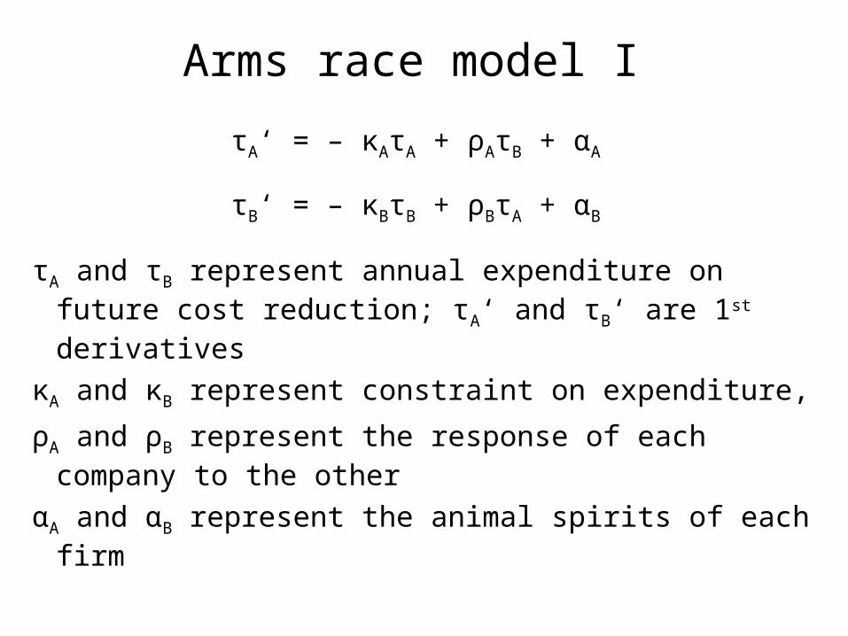
Arms race model I
τA‘ = – κAτA + ρAτB + αA
τB‘ = – κBτB + ρBτA + αB
τA and τB represent annual expenditure on future cost reduction; τA‘ and τB‘ are 1st derivatives
κA and κB represent constraint on expenditure,
ρA and ρB represent the response of each company to the other
αA and αB represent the animal spirits of each firm
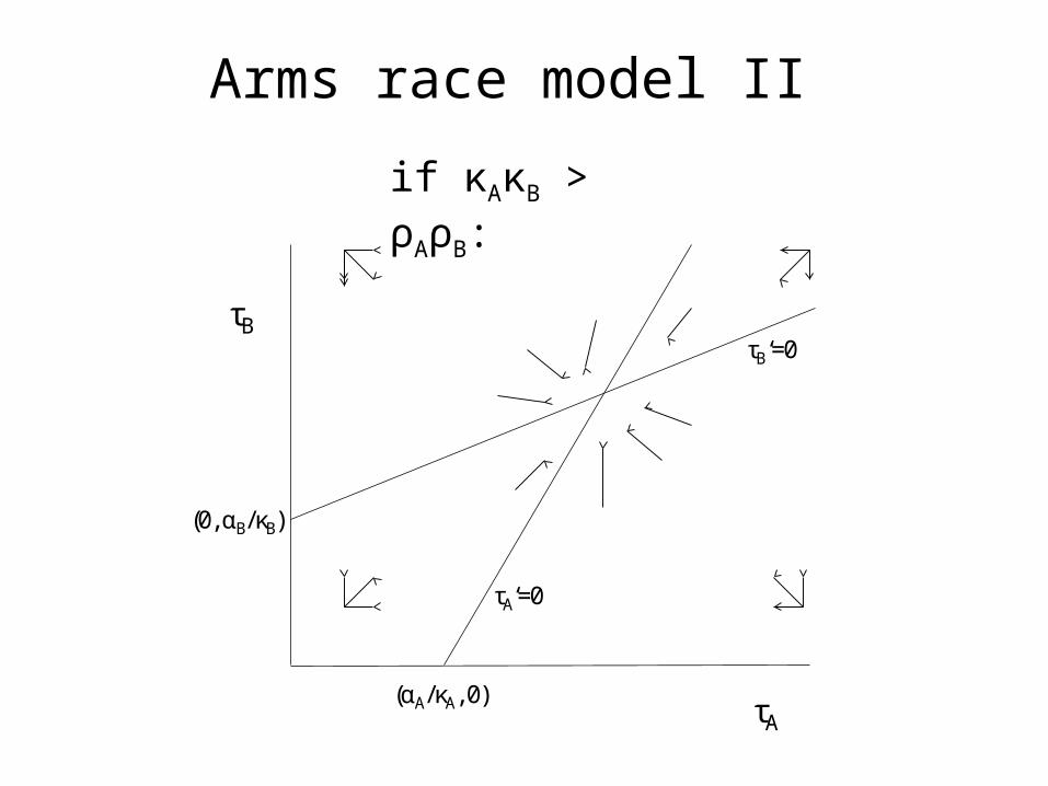
Arms race model II
τB
τA
τB‘=0
τA‘=0
(0, αB/κB)
(αA/κA, 0)
if κAκB > ρAρB:
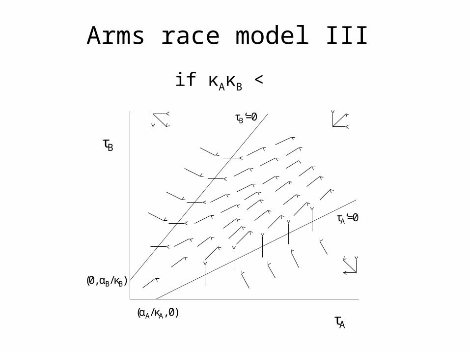
Arms race model III
if κAκB < ρAρB:
τB
τA(αA/κA, 0)
(0, αB/κB)
τA‘=0
τB‘=0

Simulations (in Vensim) • a productivity change is introduced: 10% fall in costs • each run represents a different scenario:
– baseline run, before productivity is altered (black line): everything is stable – all lines are horizontal
– innovation in a pre-capitalist economy, with no capacity to reduce costs (blue line): like the baseline, except for the initial Effect on unit cost A – a one-off effect (step change)
– competition between a capitalist and a non-capitalist firm (red line): “company” B is unable to respond to company A’s cost-cutting, leading to its relative decline
– with capitalist competition, in which both companies can reduce costs (green line): the arms race leads to greater changes in both firms than the original 10% change in productivity, and which continue indefinitely
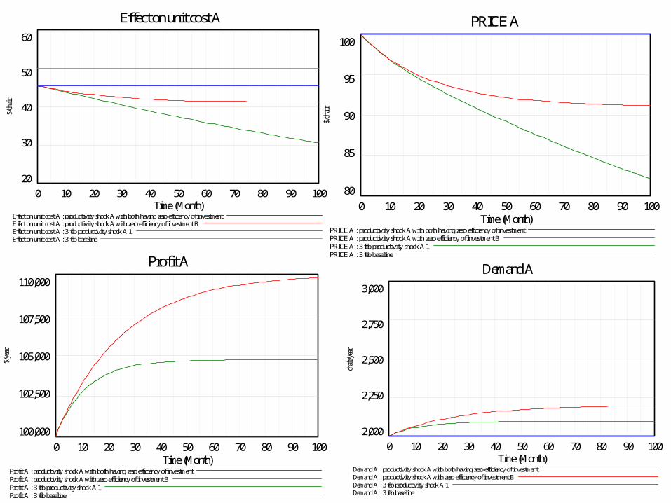
Demand A
3,000
2,750
2,500
2,250
2,000
0 10 20 30 40 50 60 70 80 90 100Time (Month)
chai
r/yea
r
Demand A : productivity shock A with both having zero efficiency of investmentDemand A : productivity shock A with zero efficiency of investment BDemand A : 3 feb productivity shock A 1Demand A : 3 feb baseline
PRICE A
100
95
90
85
80
0 10 20 30 40 50 60 70 80 90 100Time (Month)
$/ch
air
PRICE A : productivity shock A with both having zero efficiency of investmentPRICE A : productivity shock A with zero efficiency of investment BPRICE A : 3 feb productivity shock A 1PRICE A : 3 feb baseline
Profit A
110,000
107,500
105,000
102,500
100,000
0 10 20 30 40 50 60 70 80 90 100Time (Month)
$/ye
ar
Profit A : productivity shock A with both having zero efficiency of investmentProfit A : productivity shock A with zero efficiency of investment BProfit A : 3 feb productivity shock A 1Profit A : 3 feb baseline
Effect on unit cost A
60
50
40
30
20
0 10 20 30 40 50 60 70 80 90 100Time (Month)
$/ch
air
Effect on unit cost A : productivity shock A with both having zero efficiency of investmentEffect on unit cost A : productivity shock A with zero efficiency of investment BEffect on unit cost A : 3 feb productivity shock A 1Effect on unit cost A : 3 feb baseline
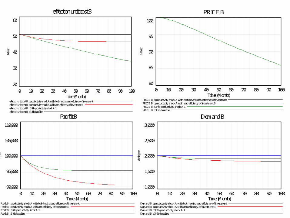
Profit B
110,000
105,000
100,000
95,000
90,000
0 10 20 30 40 50 60 70 80 90 100Time (Month)
$/ye
ar
Profit B : productivity shock A with both having zero efficiency of investmentProfit B : productivity shock A with zero efficiency of investment BProfit B : 3 feb productivity shock A 1Profit B : 3 feb baseline
PRICE B
100
95
90
85
80
0 10 20 30 40 50 60 70 80 90 100Time (Month)
$/ch
air
PRICE B : productivity shock A with both having zero efficiency of investmentPRICE B : productivity shock A with zero efficiency of investment BPRICE B : 3 feb productivity shock A 1PRICE B : 3 feb baseline
effect on unit cost B
60
50
40
30
20
0 10 20 30 40 50 60 70 80 90 100Time (Month)
$/ch
air
effect on unit cost B : productivity shock A with both having zero efficiency of investmenteffect on unit cost B : productivity shock A with zero efficiency of investment Beffect on unit cost B : 3 feb productivity shock A 1effect on unit cost B : 3 feb baseline
Demand B
3,000
2,500
2,000
1,500
1,000
0 10 20 30 40 50 60 70 80 90 100Time (Month)
chai
r/ye
ar
Demand B : productivity shock A with both having zero efficiency of investmentDemand B : productivity shock A with zero efficiency of investment BDemand B : 3 feb productivity shock A 1Demand B : 3 feb baseline

Structure of the talk
• the current discourse: – the market vs. the state – market failure
• real-economy competition between firms: – cost-tethered markets – cost competition
• free-floating markets – a model of bubbles – rationality
• conclusions
Structure of the talk
• the current discourse: – the market vs. the state – market failure
• real-economy competition between firms: – cost-tethered markets – cost competition
• free-floating markets – a model of bubbles – rationality
• conclusions
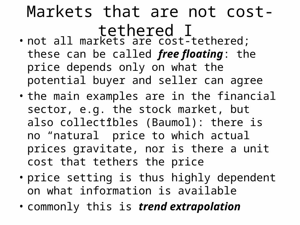
Markets that are not cost-tethered I • not all markets are cost-tethered; these can be
called free floating: the price depends only on what the potential buyer and seller can agree
• the main examples are in the financial sector, e.g. the stock market, but also collectibles (Baumol): there is no “natural” price to which actual prices gravitate, nor is there a unit cost that tethers the price
• price setting is thus highly dependent on what information is available
• commonly this is trend extrapolation
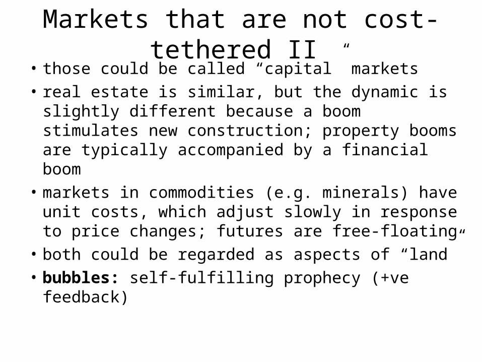
Markets that are not cost-tethered II • those could be called “capital” markets • real estate is similar, but the dynamic is slightly
different because a boom stimulates new construction; property booms are typically accompanied by a financial boom
• markets in commodities (e.g. minerals) have unit costs, which adjust slowly in response to price changes; futures are free-floating
• both could be regarded as aspects of “land” • bubbles: self-fulfilling prophecy (+ve feedback)
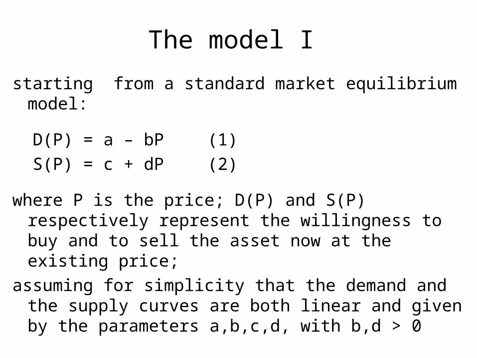
The model I
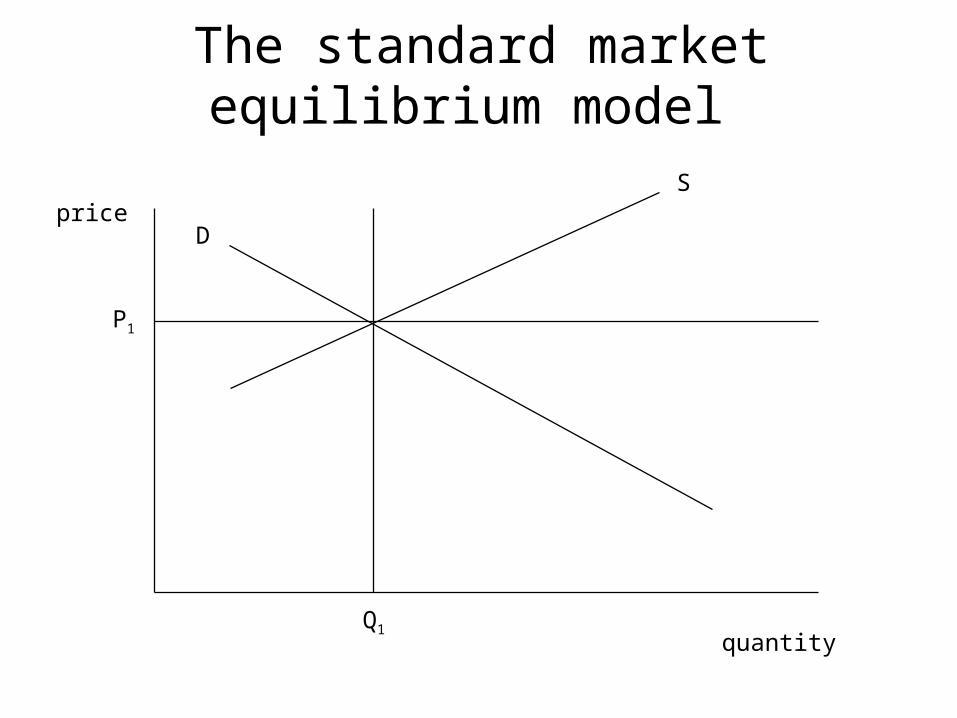
starting from a standard market equilibrium model:
D(P) = a – bP (1) S(P) = c + dP (2)
where P is the price; D(P) and S(P) respectively represent the willingness to buy and to sell the asset now at the existing price;
assuming for simplicity that the demand and the supply curves are both linear and given by the parameters a,b,c,d, with b,d > 0

The standard market equilibrium model
price
quantity
P1
Q1
D
S
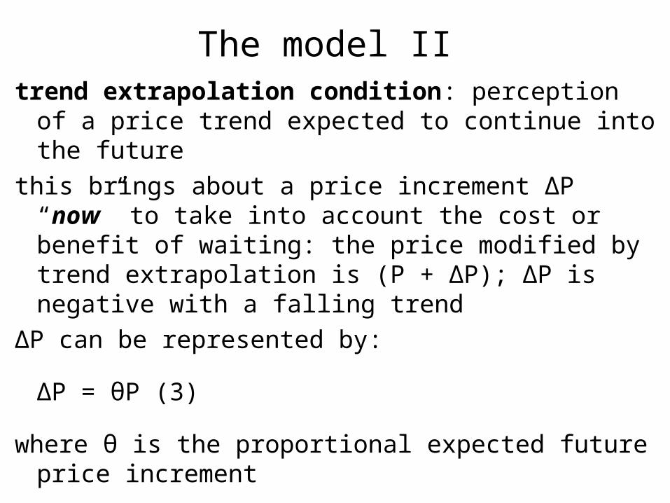
The model II trend extrapolation condition: perception of a
price trend expected to continue into the future
this brings about a price increment ΔP “now” to take into account the cost or benefit of waiting: the price modified by trend extrapolation is (P + ΔP); ΔP is negative with a falling trend
ΔP can be represented by:
ΔP = θP (3)
where θ is the proportional expected future price increment
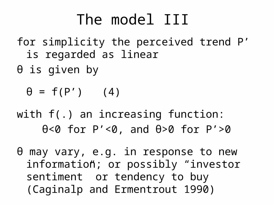
The model III
for simplicity the perceived trend P’ is regarded as linear
θ is given by
θ = f(P’) (4)
with f(.) an increasing function:
θ<0 for P’<0, and θ>0 for P’>0
θ may vary, e.g. in response to new information; or possibly “investor sentiment” or tendency to buy (Caginalp and Ermentrout 1990)
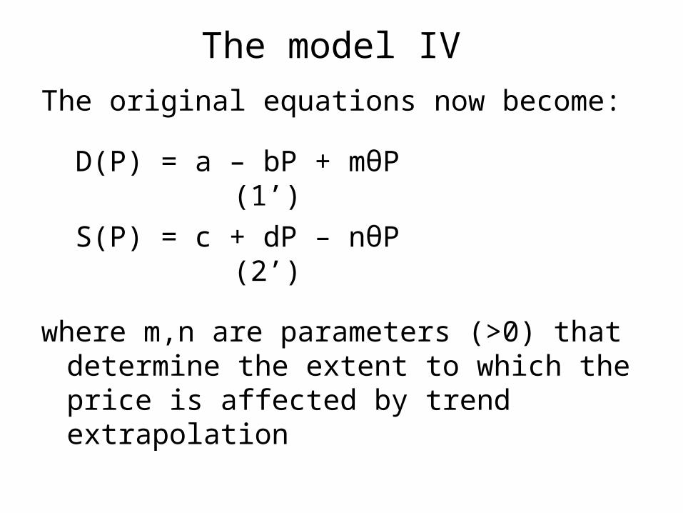
The model IV
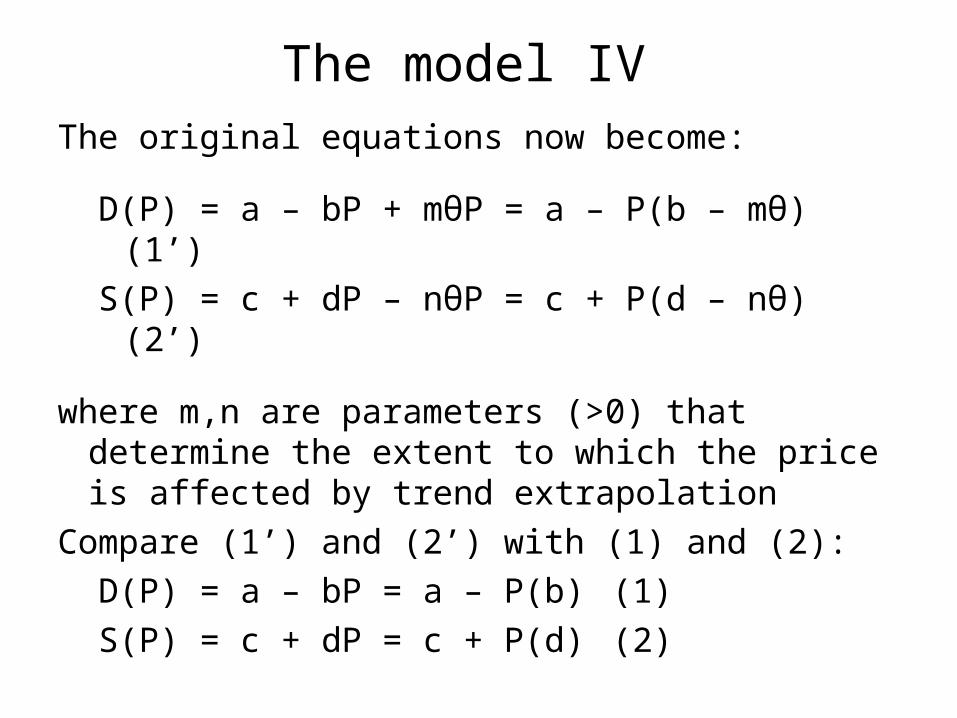
The original equations now become:
D(P) = a – bP + mθP (1’)
S(P) = c + dP – nθP (2’)
where m,n are parameters (>0) that determine the extent to which the price is affected by trend extrapolation
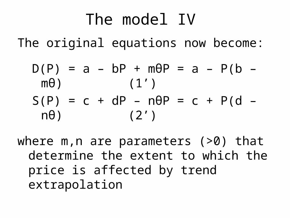
The model IV
The original equations now become:
D(P) = a – bP + mθP = a – P(b – mθ) (1’) S(P) = c + dP – nθP = c + P(d – nθ) (2’)
where m,n are parameters (>0) that determine the extent to which the price is affected by trend extrapolation
The model IV
The original equations now become:
D(P) = a – bP + mθP = a – P(b – mθ) (1’) S(P) = c + dP – nθP = c + P(d – nθ) (2’)
where m,n are parameters (>0) that determine the extent to which the price is affected by trend extrapolation
Compare (1’) and (2’) with (1) and (2):
D(P) = a – bP (1) S(P) = c + dP (2)
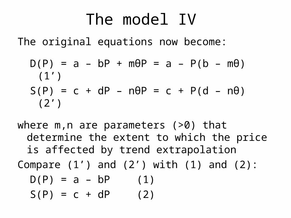
The model IV
The original equations now become:
D(P) = a – bP + mθP = a – P(b – mθ) (1’) S(P) = c + dP – nθP = c + P(d – nθ) (2’)
where m,n are parameters (>0) that determine the extent to which the price is affected by trend extrapolation
Compare (1’) and (2’) with (1) and (2):
D(P) = a – bP = a – P(b) (1) S(P) = c + dP = c + P(d) (2)
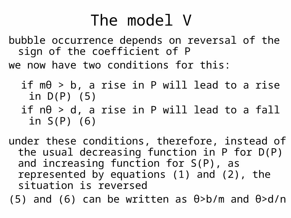
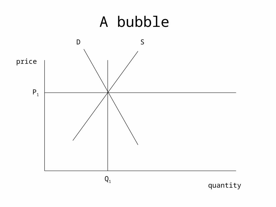
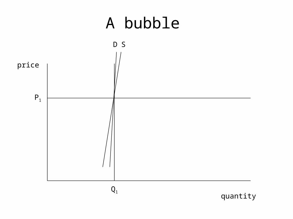
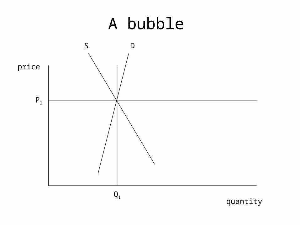
The model V bubble occurrence depends on reversal of the sign
of the coefficient of P we now have two conditions for this:
if mθ > b, a rise in P will lead to a rise in D(P) (5) if nθ > d, a rise in P will lead to a fall in S(P) (6)
under these conditions, therefore, instead of the usual decreasing function in P for D(P) and increasing function for S(P), as represented by equations (1) and (2), the situation is reversed
(5) and (6) can be written as θ>b/m and θ>d/n
The standard market equilibrium model
price
quantity
P1
Q1
D
S
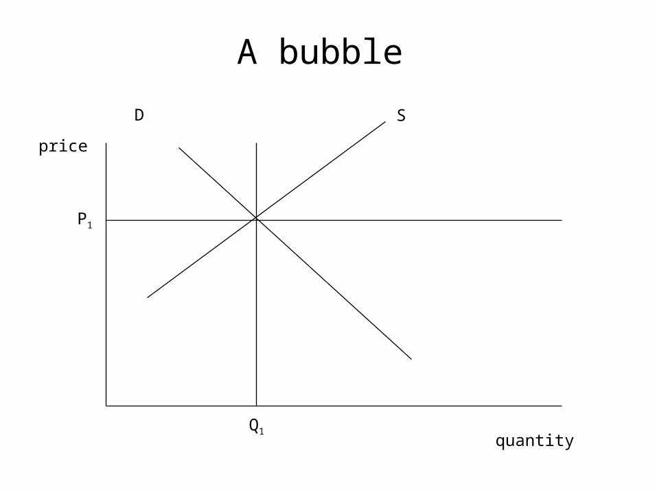
A bubble
price
quantity
P1
Q1
D S
A bubble
price
quantity
P1
Q1
D S
A bubble
price
quantity
P1
Q1
D S
A bubble
price
quantity
P1
Q1
DS
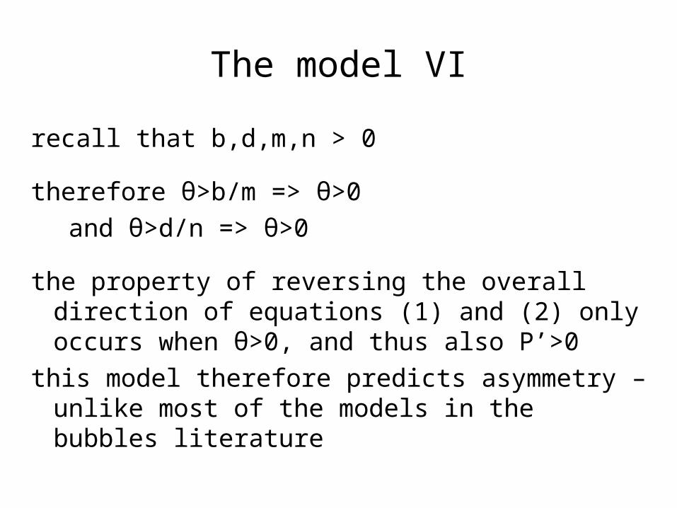
The model VI
recall that b,d,m,n > 0
therefore θ>b/m => θ>0
and θ>d/n => θ>0
the property of reversing the overall direction of equations (1) and (2) only occurs when θ>0, and thus also P’>0
this model therefore predicts asymmetry – unlike most of the models in the bubbles literature
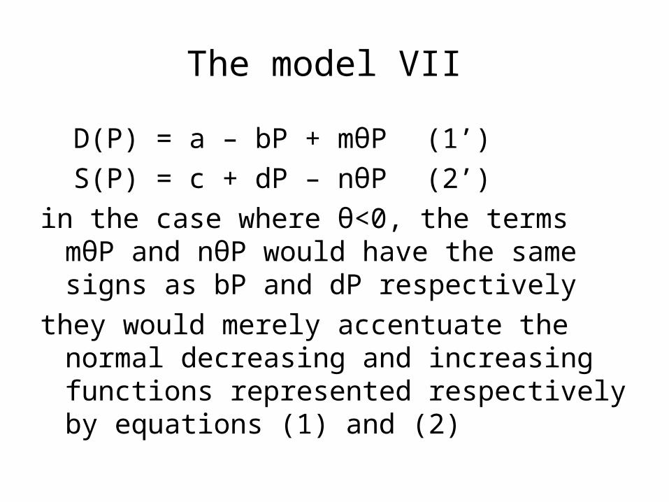
The model VII
D(P) = a – bP + mθP (1’) S(P) = c + dP – nθP (2’)
in the case where θ<0, the terms mθP and nθP would have the same signs as bP and dP respectively
they would merely accentuate the normal decreasing and increasing functions represented respectively by equations (1) and (2)
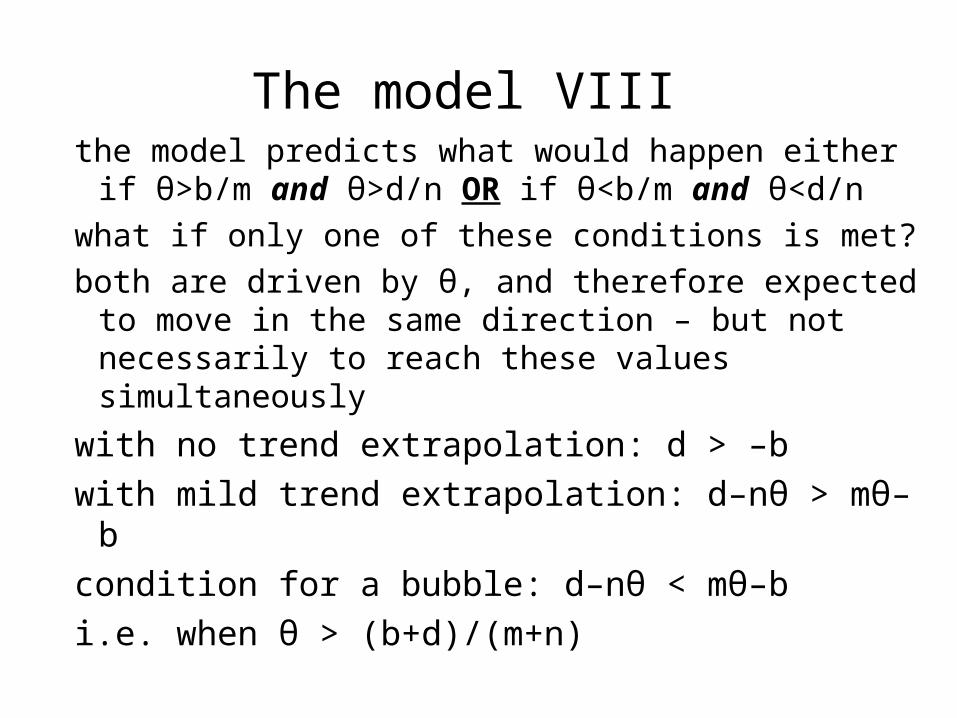
The model VIII the model predicts what would happen either if
θ>b/m and θ>d/n OR if θ<b/m and θ<d/n what if only one of these conditions is met? both are driven by θ, and therefore expected to
move in the same direction – but not necessarily to reach these values simultaneously
with no trend extrapolation: d > –b with mild trend extrapolation: d–nθ > mθ–b condition for a bubble: d–nθ < mθ–b i.e. when θ > (b+d)/(m+n)
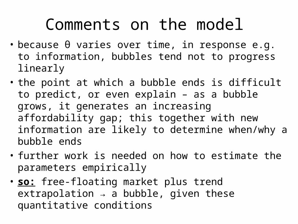
Comments on the model • because θ varies over time, in response e.g. to
information, bubbles tend not to progress linearly
• the point at which a bubble ends is difficult to predict, or even explain – as a bubble grows, it generates an increasing affordability gap; this together with new information are likely to determine when/why a bubble ends
• further work is needed on how to estimate the parameters empirically
• so: free-floating market plus trend extrapolation → a bubble, given these quantitative conditions

Structure of the talk
• the current discourse: – the market vs. the state – market failure
• real-economy competition between firms: – cost-tethered markets – cost competition
• free-floating markets – a model of bubbles – rationality
• conclusions
Structure of the talk
• the current discourse: – the market vs. the state – market failure
• real-economy competition between firms: – cost-tethered markets – cost competition
• free-floating markets – a model of bubbles – rationality
• conclusions
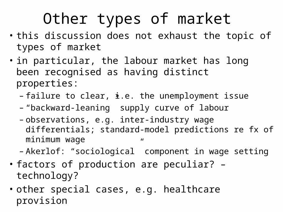
Other types of market • this discussion does not exhaust the topic of types
of market • in particular, the labour market has long been
recognised as having distinct properties: – failure to clear, i.e. the unemployment issue – “backward-leaning” supply curve of labour – observations, e.g. inter-industry wage differentials;
standard-model predictions re fx of minimum wage – Akerlof: “sociological” component in wage setting
• factors of production are peculiar? – technology? • other special cases, e.g. healthcare provision
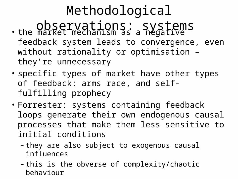
Methodological observations: systems • the market mechanism as a negative feedback
system leads to convergence, even without rationality or optimisation – they’re unnecessary
• specific types of market have other types of feedback: arms race, and self-fulfilling prophecy
• Forrester: systems containing feedback loops generate their own endogenous causal processes that make them less sensitive to initial conditions – they are also subject to exogenous causal influences – this is the obverse of complexity/chaotic behaviour
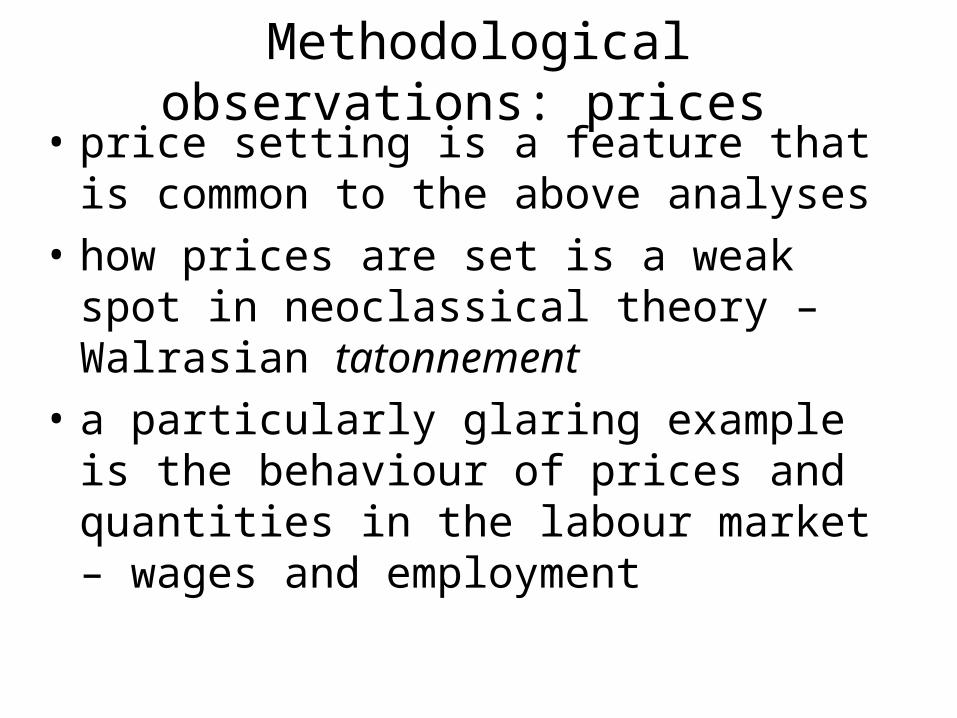
Methodological observations: prices • price setting is a feature that is common to the
above analyses • how prices are set is a weak spot in neoclassical
theory – Walrasian tatonnement • a particularly glaring example is the behaviour
of prices and quantities in the labour market – wages and employment
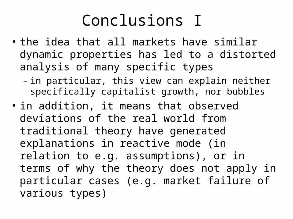
Conclusions I • the idea that all markets have similar dynamic
properties has led to a distorted analysis of many specific types – in particular, this view can explain neither
specifically capitalist growth, nor bubbles
• in addition, it means that observed deviations of the real world from traditional theory have generated explanations in reactive mode (in relation to e.g. assumptions), or in terms of why the theory does not apply in particular cases (e.g. market failure of various types)
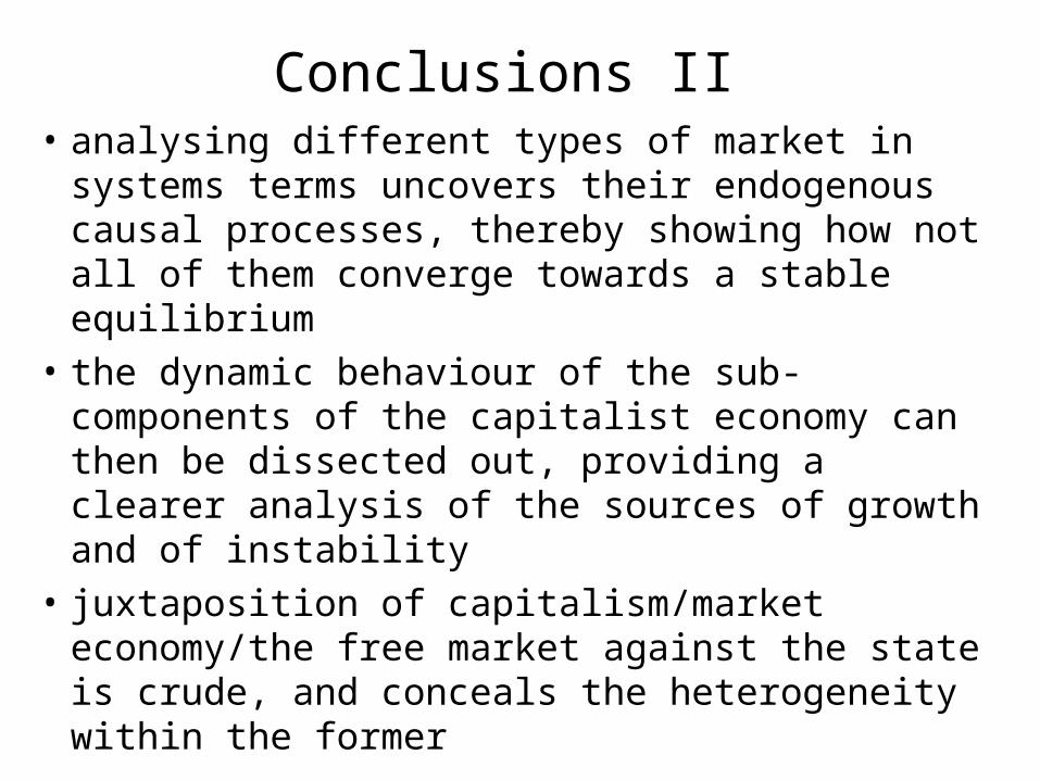
Conclusions II • analysing different types of market in systems
terms uncovers their endogenous causal processes, thereby showing how not all of them converge towards a stable equilibrium
• the dynamic behaviour of the sub-components of the capitalist economy can then be dissected out, providing a clearer analysis of the sources of growth and of instability
• juxtaposition of capitalism/market economy/the free market against the state is crude, and conceals the heterogeneity within the former

Thank you!
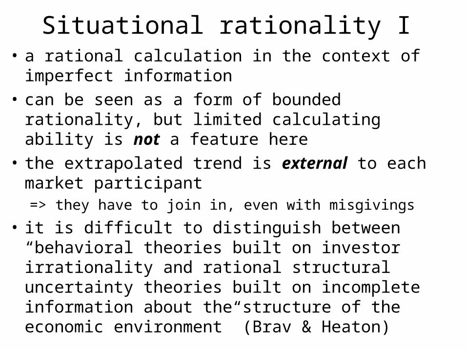
Situational rationality I • a rational calculation in the context of imperfect
information
• can be seen as a form of bounded rationality, but limited calculating ability is not a feature here
• the extrapolated trend is external to each market participant => they have to join in, even with misgivings
• it is difficult to distinguish between “behavioral theories built on investor irrationality and rational structural uncertainty theories built on incomplete information about the structure of the economic environment” (Brav & Heaton)
Situational rationality II
• Caginalp & Ermentrout: “emotional”; also “group-think”, “optimism” or “panic” • e.g. Akerlof & Shiller: “Animal spirits”


Situational rationality II
• Caginalp & Ermentrout: “emotional”; also “group-think”, “optimism” or “panic” • e.g. Akerlof & Shiller: “Animal spirits”
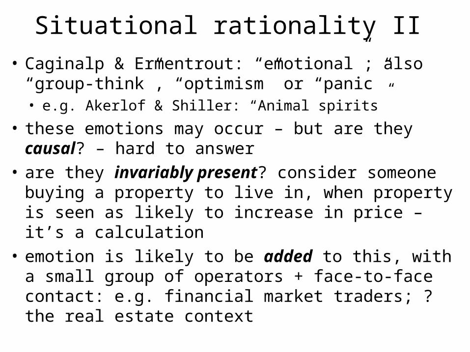
Situational rationality II
• Caginalp & Ermentrout: “emotional”; also “group-think”, “optimism” or “panic” • e.g. Akerlof & Shiller: “Animal spirits”
• these emotions may occur – but are they causal? – hard to answer
• are they invariably present? consider someone buying a property to live in, when property is seen as likely to increase in price – it’s a calculation
• emotion is likely to be added to this, with a small group of operators + face-to-face contact: e.g. financial market traders; ? the real estate context