Embed Size (px)
Citation preview
How to weigh the Milky Way using tidal tails of globular clusters
Andreas H.W. Küpper
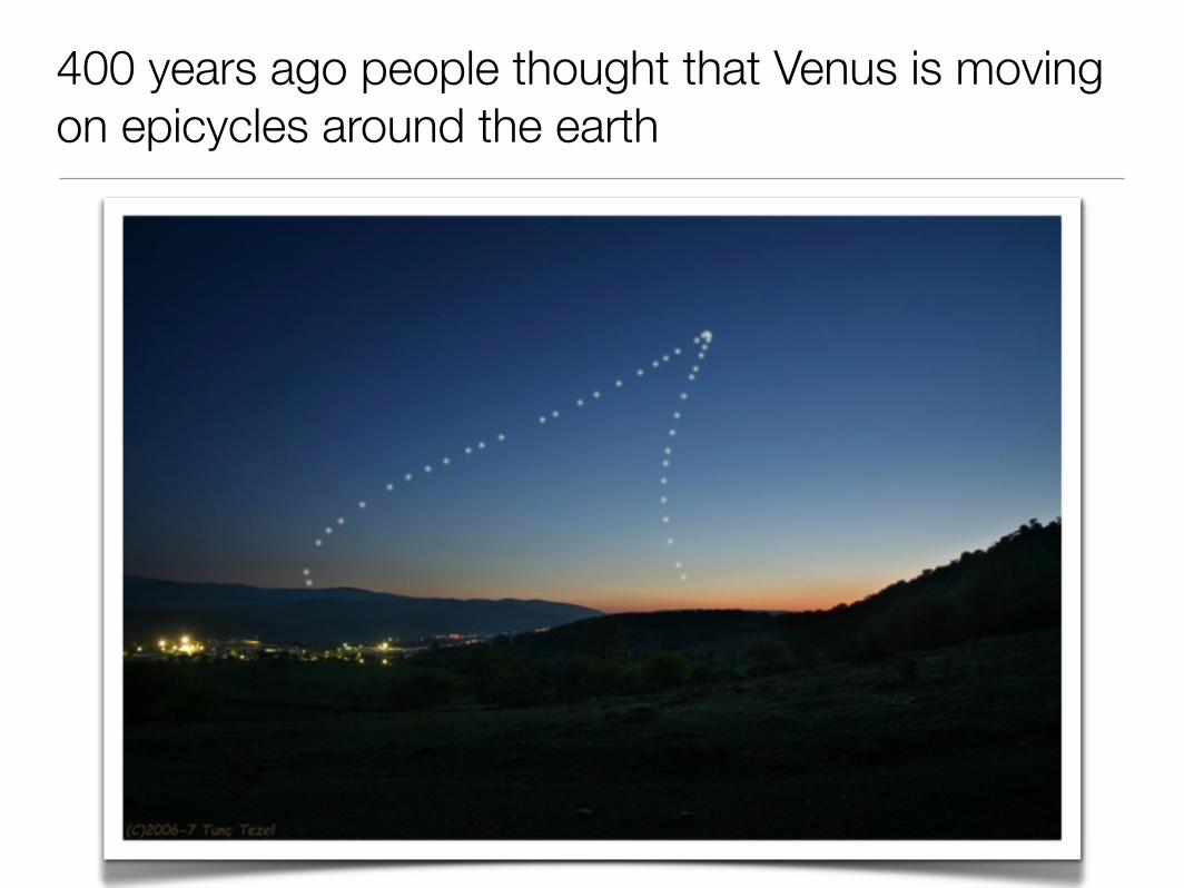
400 years ago people thought that Venus is moving on epicycles around the earth
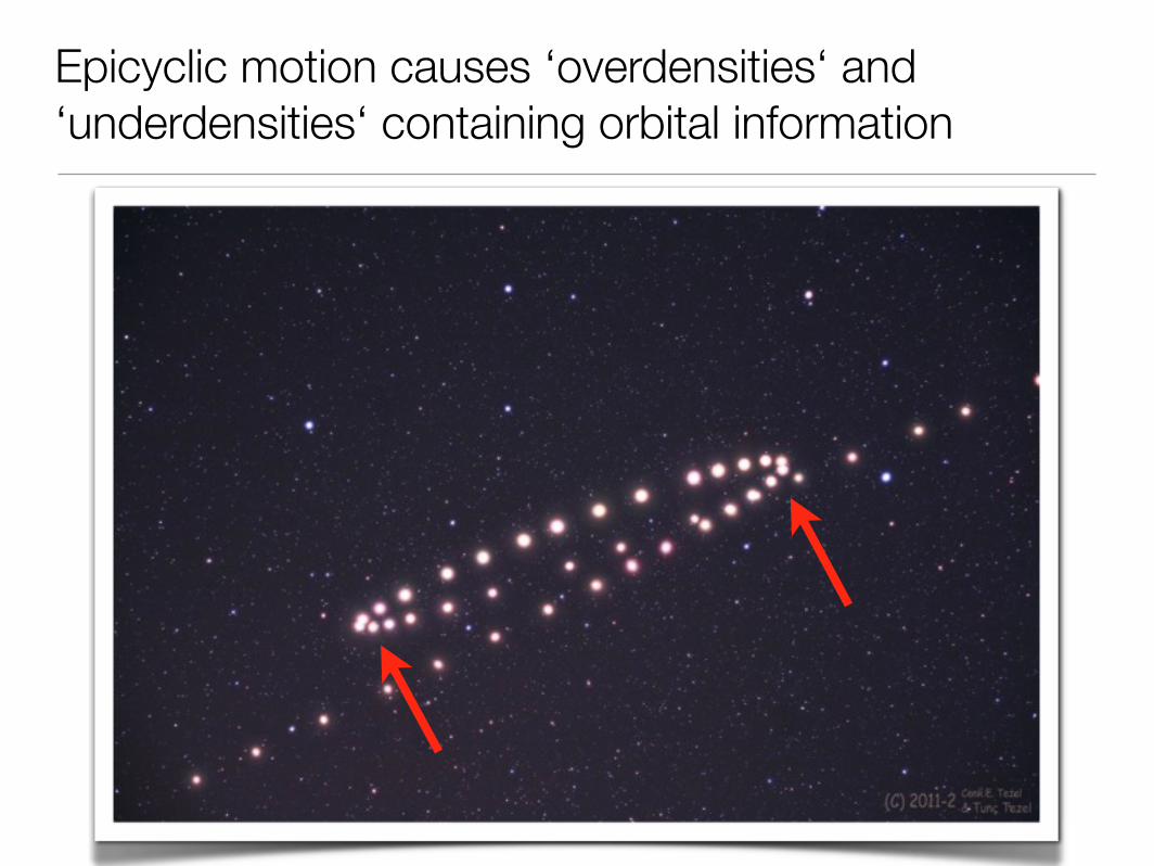
Epicyclic motion causes ‘overdensities‘ and ‘underdensities‘ containing orbital information
X
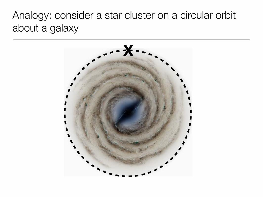
Analogy: consider a star cluster on a circular orbit about a galaxy
X
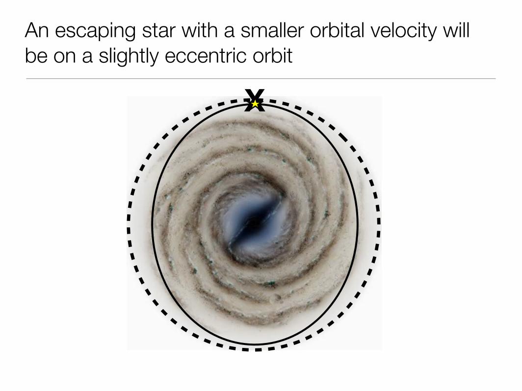
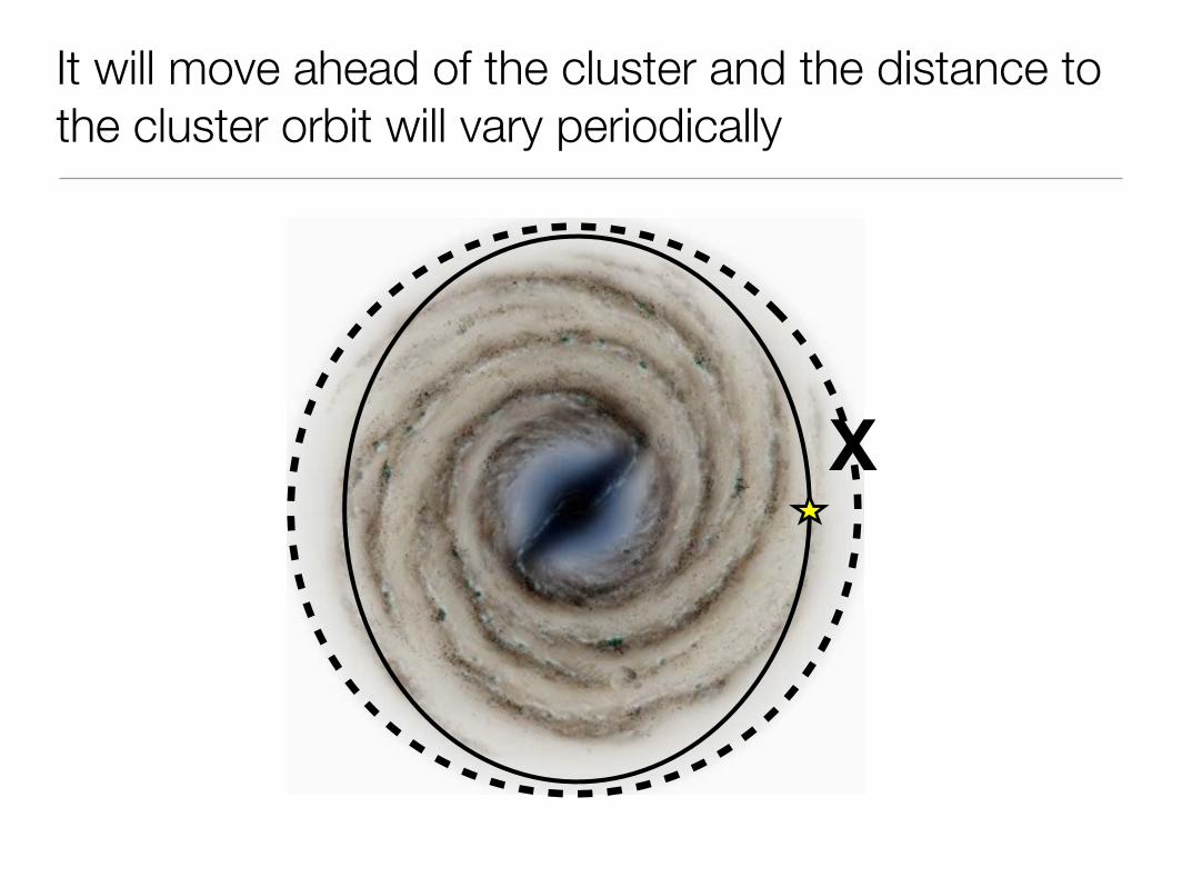
An escaping star with a smaller orbital velocity will be on a slightly eccentric orbit
X
It will move ahead of the cluster and the distance to the cluster orbit will vary periodically
X
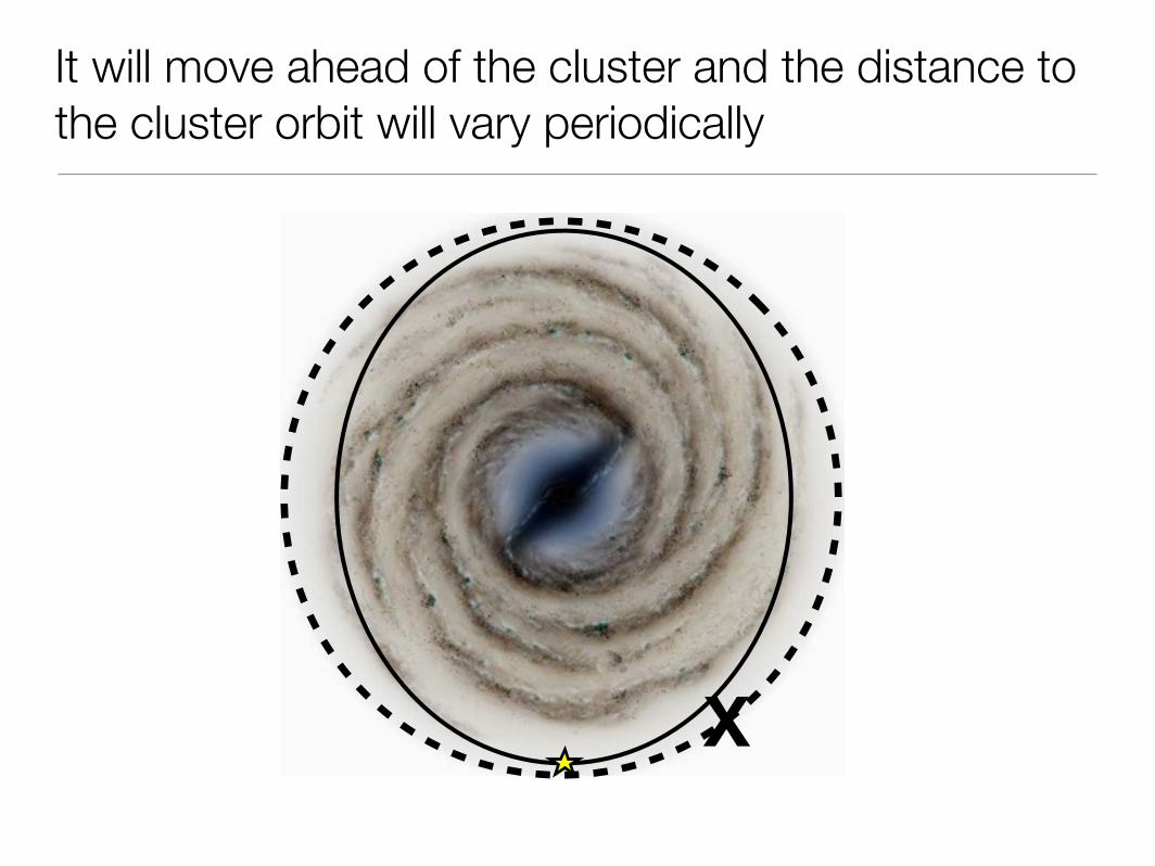
It will move ahead of the cluster and the distance to the cluster orbit will vary periodically
X
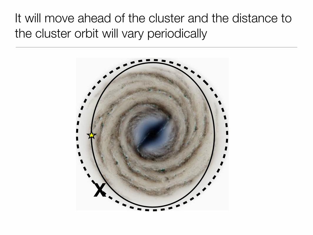
It will move ahead of the cluster and the distance to the cluster orbit will vary periodically
X
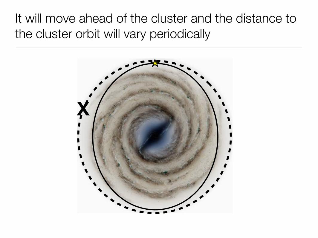
It will move ahead of the cluster and the distance to the cluster orbit will vary periodically
x
y
x
z
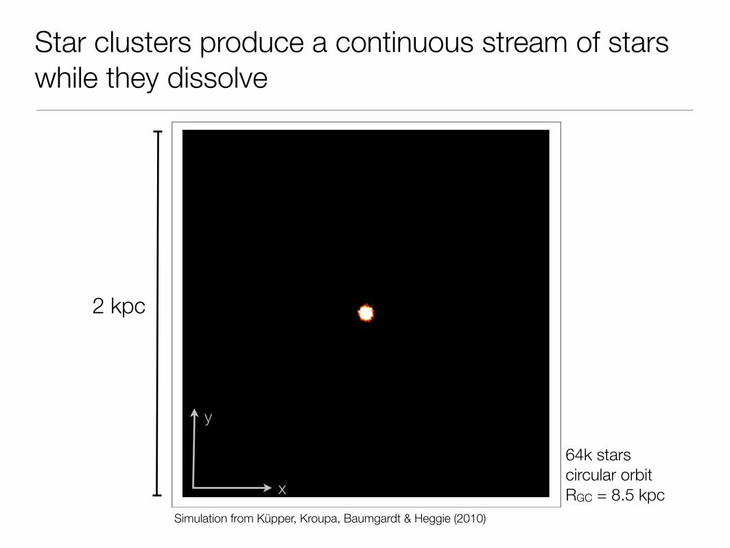
Simulation from Küpper, Kroupa, Baumgardt & Heggie (2010)
64k starscircular orbitRGC = 8.5 kpc
Star clusters produce a continuous stream of stars while they dissolve
2 kpc
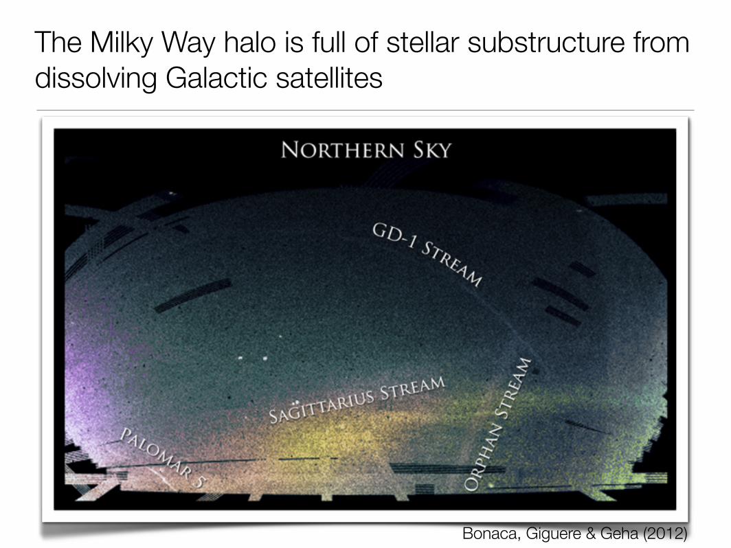
The Milky Way halo is full of stellar substructure from dissolving Galactic satellites
Bonaca, Giguere & Geha (2012)
11
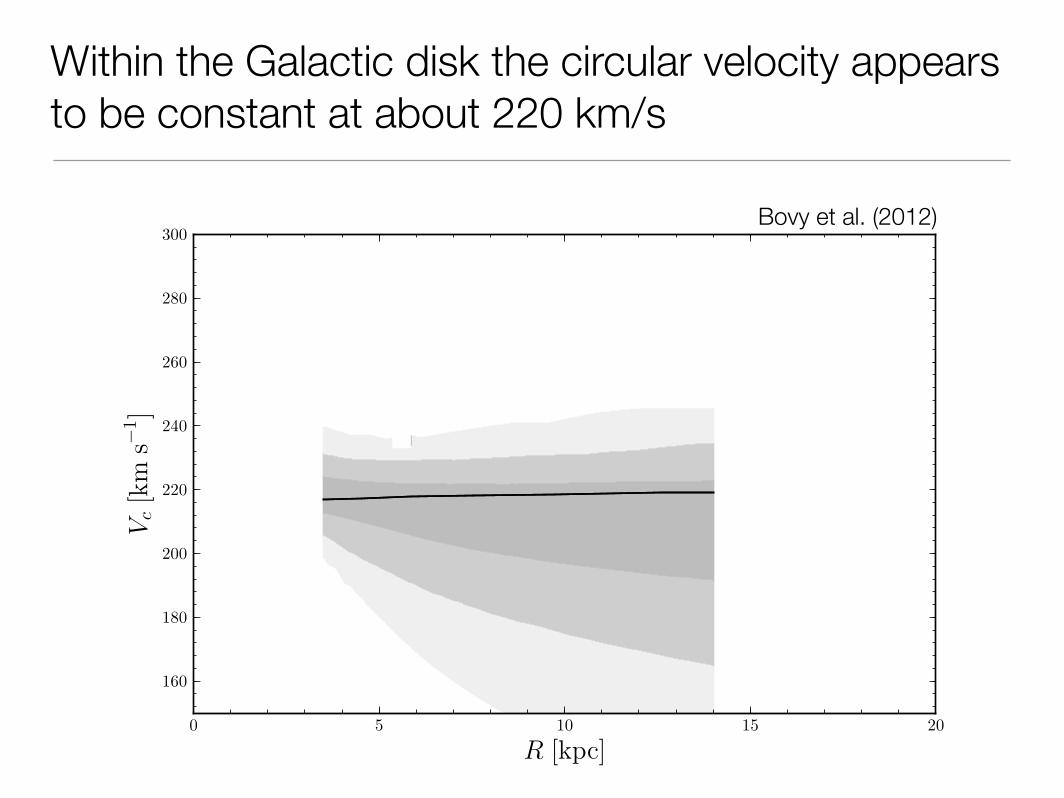
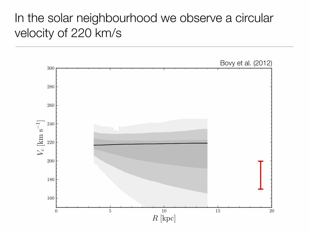
Fig. 6.— The MilkyWay’s rotation curve in the range 4< R < 14kpc as inferred from our data for di!erent forms of the shape of therotation curve. At each R, the range in Vc(R) from 10,000 samplesof the PDF—assuming a power-law or cubic-polynomial model forthe shape of the rotation curve—is determined and the 68%, 95%,and 99% intervals are shown in varying shades of gray. For thecubic-polynomial model, we impose a prior that R0 < 9 kpc (seetext). For comparison, the squares show the rotation curve of M31from the compilation of Carignan et al. (2006).
V!,! = 242+5"17 km s"1 (for a power-law fit to the rota-
tion curve). In the latter fit, there is a strong correlationbetween Vc and V!,!; the di!erence between the two ismuch better constrained: V!,! ! Vc = 23.1+3.6
"0.5 km s"1.The marginalized PDF for V!,! ! Vc in FIG. 5 is well-described by V!,! ! Vc = 26± 3 km s"1. We discuss theconsequences of this solar motion in detail in § 5.3, butwe note here that the estimate of the angular motion ofthe Galactic center that we obtain from combining ourfits for V!,! and R0 is consistent with the proper motionof Sgr A# as measured by Reid & Brunthaler (2004): ourestimate is µSgr A! = 6.3+0.1
"0.7mas yr"1, compared to thedirect measurement of 6.379 ± 0.024mas yr"1. We dis-cuss the apparent discrepancy between our agreementwith the proper motion of Sgr A# and our low value forVc in § 5.3.The final block of parameters in TABLE 2 describe
the tracer population. The velocity dispersion that weinfer for the tracer stars is close to that expected foran old disk population: !R(R0) " 32.0+0.5
"3 km s"1 forthe flat-rotation-curve and power-law fits. The ratio ofthe tangential-to-radial velocity dispersions squared is0.69 < X2 < 1.0, with the best-fit value at the lower end
of this range. This value is higher than expected fromthe epicycle approximation for a flat or falling rotationcurve, which is X2 # 0.5. However, this expectationholds only for a cold disk, and corrections due to thetemperature of the old disk population always increaseX2 near R0 (Kuijken & Tremaine 1991): the Dehnendisk distribution functions of Equation (6) have X2 thatvaries spatially, and reaches approximately 0.65 near R0(Dehnen 1999). The best-fit value for R0/h" is approx-imately zero, with non-zero positive values ruled out bythe data: the 68% interval is !0.24 < R0/h" < 0.03.Thus, the radial-velocity dispersion does not drop expo-nentially with radius with a scale length between 2R0/3and R0; such a drop would be expected from previ-ous measurements of the radial dispersion as a func-tion of R (Lewis & Freeman 1989), or from the observedexponential decline of the vertical velocity dispersion(Bovy et al. 2012b) combined with the assumption ofconstant !z/!R. We have attempted fits with two popu-lations of stars with di!erent radial scale lengths (3 kpcand 5 or 6 kpc) and radial-velocity dispersions, but thesame radial-dispersion scale length. The best-fit R0/h"remains zero, such that it does not seem that we are see-ing a mix of multiple populations that conspire to forma flat !R profile.Even with the best-fit flat radial-dispersion profile, the
disk is stable over most of the range in R consideredhere. The Toomre Q parameter—Q = !R "/(3.36G")(Toomre 1964)—for a flat rotation curve is
Q = 1.72
!
!R
32 km s"1
" !
Vc
220 km s"1
"
!
R
8 kpc
""1 !
"
50M! pc"2
""1
.
(9)
This expression has Q > 1 down to 4.9 kpc and Q = 0.91at R = 4 kpc for a constant !R(R) and a surface den-sity " $ e"R/(3 kpc). Although the disk is marginallyunstable in our best-fit model, this conclusion dependsstrongly on the assumed radial scale length: for hR =3.25 kpc, Q > 1 everywhere at R > 4 kpc. The flat-ness of the inferred !R profile also depends on the as-sumed constancy of X2. Actual equilibrium axisymmet-ric disks, such as those having a Dehnen distributionfunction (Equation (6)), have a radially-dependent X2,with X2 at R = 4 kpc typically smaller than at R = 8 to16 kpc (Dehnen 1999, Figure 4). AtR = 4 kpc, which forthe present data sample is only reached for the l = 30$
line of sight, the line-of-sight velocity is entirely com-posed of the tangential-velocity component, such thatany decrease in X2 leads to an increase in !R to sustainthe same !!. Therefore, the true !R(R) profile presum-ably is falling with R, and the entire disk at R > 4 kpcshould be stable in our model.Full PDFs for all of the parameters of the basic models
discussed in this section are given in FIG. 5. It is clearthat with the exception of Vc and the derivative of therotation curve—# in the power-law model and dVc/dRin the linear model—there are no strong degeneraciesamong the parameters. Also included in this figure arethe results from fitting all but one of the 14 APOGEEfield for each field: these leave-one-out results show thatno single field drives the analysis for any of the parame-
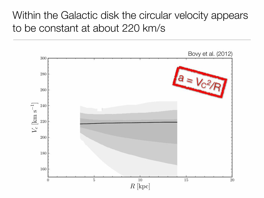
Within the Galactic disk the circular velocity appears to be constant at about 220 km/s
Bovy et al. (2012)
11
Fig. 6.— The MilkyWay’s rotation curve in the range 4< R < 14kpc as inferred from our data for di!erent forms of the shape of therotation curve. At each R, the range in Vc(R) from 10,000 samplesof the PDF—assuming a power-law or cubic-polynomial model forthe shape of the rotation curve—is determined and the 68%, 95%,and 99% intervals are shown in varying shades of gray. For thecubic-polynomial model, we impose a prior that R0 < 9 kpc (seetext). For comparison, the squares show the rotation curve of M31from the compilation of Carignan et al. (2006).
V!,! = 242+5"17 km s"1 (for a power-law fit to the rota-
tion curve). In the latter fit, there is a strong correlationbetween Vc and V!,!; the di!erence between the two ismuch better constrained: V!,! ! Vc = 23.1+3.6
"0.5 km s"1.The marginalized PDF for V!,! ! Vc in FIG. 5 is well-described by V!,! ! Vc = 26± 3 km s"1. We discuss theconsequences of this solar motion in detail in § 5.3, butwe note here that the estimate of the angular motion ofthe Galactic center that we obtain from combining ourfits for V!,! and R0 is consistent with the proper motionof Sgr A# as measured by Reid & Brunthaler (2004): ourestimate is µSgr A! = 6.3+0.1
"0.7mas yr"1, compared to thedirect measurement of 6.379 ± 0.024mas yr"1. We dis-cuss the apparent discrepancy between our agreementwith the proper motion of Sgr A# and our low value forVc in § 5.3.The final block of parameters in TABLE 2 describe
the tracer population. The velocity dispersion that weinfer for the tracer stars is close to that expected foran old disk population: !R(R0) " 32.0+0.5
"3 km s"1 forthe flat-rotation-curve and power-law fits. The ratio ofthe tangential-to-radial velocity dispersions squared is0.69 < X2 < 1.0, with the best-fit value at the lower end
of this range. This value is higher than expected fromthe epicycle approximation for a flat or falling rotationcurve, which is X2 # 0.5. However, this expectationholds only for a cold disk, and corrections due to thetemperature of the old disk population always increaseX2 near R0 (Kuijken & Tremaine 1991): the Dehnendisk distribution functions of Equation (6) have X2 thatvaries spatially, and reaches approximately 0.65 near R0(Dehnen 1999). The best-fit value for R0/h" is approx-imately zero, with non-zero positive values ruled out bythe data: the 68% interval is !0.24 < R0/h" < 0.03.Thus, the radial-velocity dispersion does not drop expo-nentially with radius with a scale length between 2R0/3and R0; such a drop would be expected from previ-ous measurements of the radial dispersion as a func-tion of R (Lewis & Freeman 1989), or from the observedexponential decline of the vertical velocity dispersion(Bovy et al. 2012b) combined with the assumption ofconstant !z/!R. We have attempted fits with two popu-lations of stars with di!erent radial scale lengths (3 kpcand 5 or 6 kpc) and radial-velocity dispersions, but thesame radial-dispersion scale length. The best-fit R0/h"remains zero, such that it does not seem that we are see-ing a mix of multiple populations that conspire to forma flat !R profile.Even with the best-fit flat radial-dispersion profile, the
disk is stable over most of the range in R consideredhere. The Toomre Q parameter—Q = !R "/(3.36G")(Toomre 1964)—for a flat rotation curve is
Q = 1.72
!
!R
32 km s"1
" !
Vc
220 km s"1
"
!
R
8 kpc
""1 !
"
50M! pc"2
""1
.
(9)
This expression has Q > 1 down to 4.9 kpc and Q = 0.91at R = 4 kpc for a constant !R(R) and a surface den-sity " $ e"R/(3 kpc). Although the disk is marginallyunstable in our best-fit model, this conclusion dependsstrongly on the assumed radial scale length: for hR =3.25 kpc, Q > 1 everywhere at R > 4 kpc. The flat-ness of the inferred !R profile also depends on the as-sumed constancy of X2. Actual equilibrium axisymmet-ric disks, such as those having a Dehnen distributionfunction (Equation (6)), have a radially-dependent X2,with X2 at R = 4 kpc typically smaller than at R = 8 to16 kpc (Dehnen 1999, Figure 4). AtR = 4 kpc, which forthe present data sample is only reached for the l = 30$
line of sight, the line-of-sight velocity is entirely com-posed of the tangential-velocity component, such thatany decrease in X2 leads to an increase in !R to sustainthe same !!. Therefore, the true !R(R) profile presum-ably is falling with R, and the entire disk at R > 4 kpcshould be stable in our model.Full PDFs for all of the parameters of the basic models
discussed in this section are given in FIG. 5. It is clearthat with the exception of Vc and the derivative of therotation curve—# in the power-law model and dVc/dRin the linear model—there are no strong degeneraciesamong the parameters. Also included in this figure arethe results from fitting all but one of the 14 APOGEEfield for each field: these leave-one-out results show thatno single field drives the analysis for any of the parame-
Within the Galactic disk the circular velocity appears to be constant at about 220 km/s
Bovy et al. (2012)
a = VC 2/R
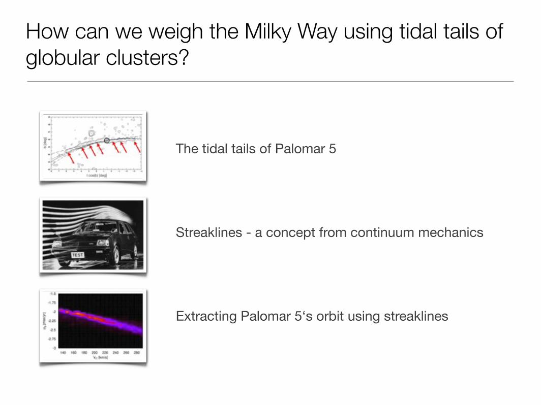
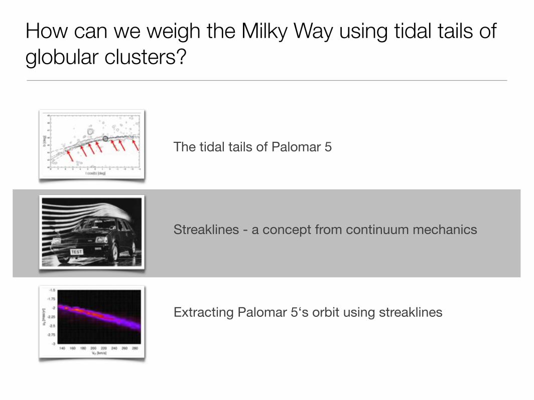
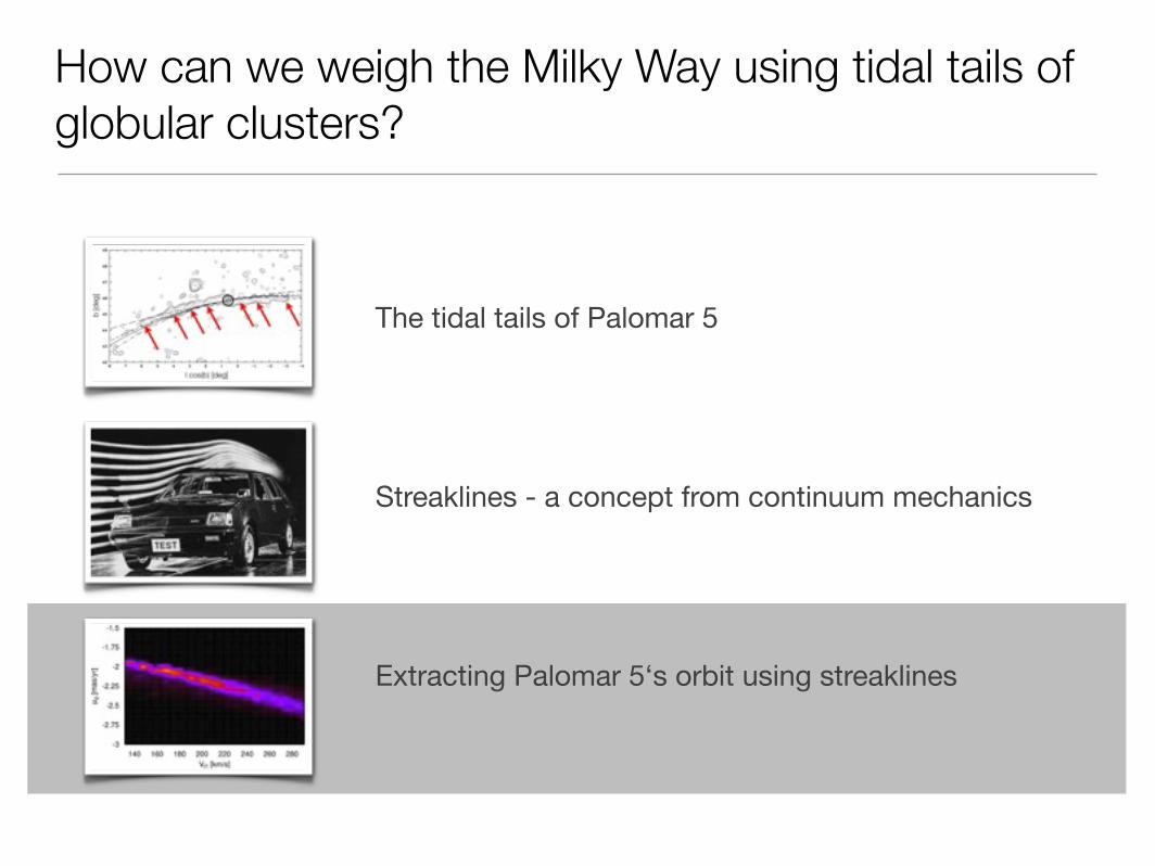
How can we weigh the Milky Way using tidal tails of globular clusters?
The tidal tails of Palomar 5
Streaklines - a concept from continuum mechanics
Extracting Palomar 5‘s orbit using streaklines
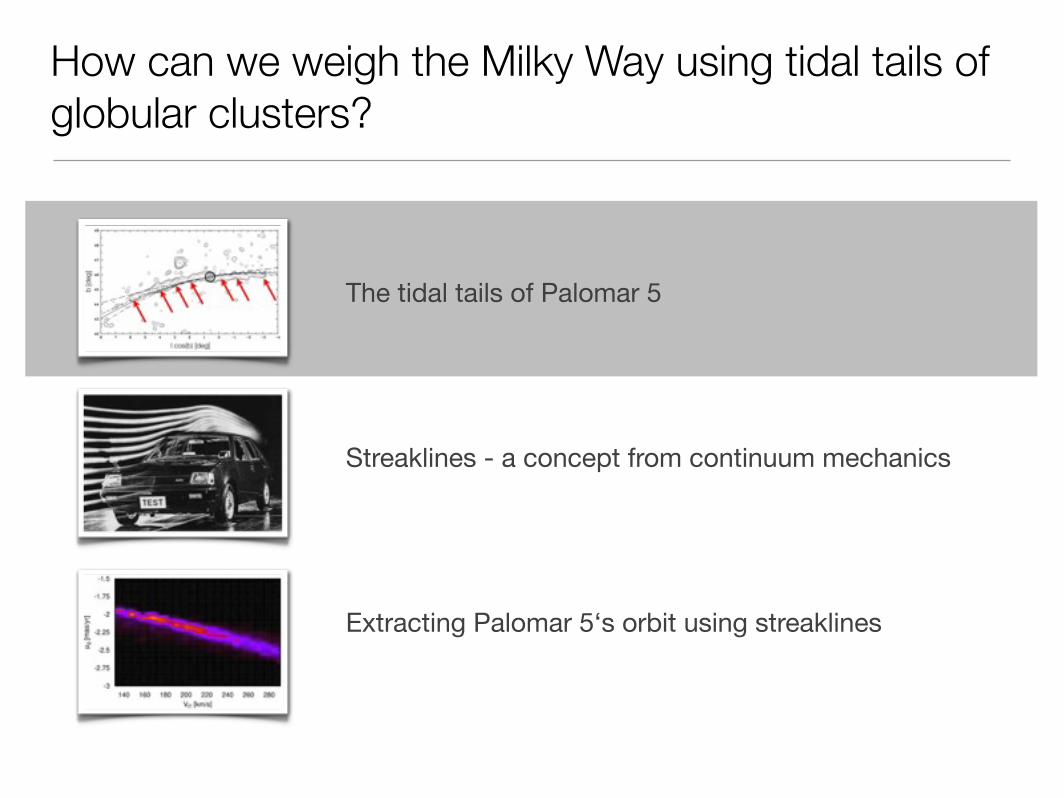
How can we weigh the Milky Way using tidal tails of globular clusters?
The tidal tails of Palomar 5
Streaklines - a concept from continuum mechanics
Extracting Palomar 5‘s orbit using streaklines
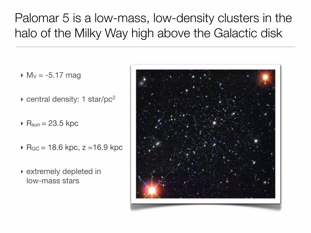
Palomar 5 is a low-mass, low-density clusters in the halo of the Milky Way high above the Galactic disk
‣ MV = -5.17 mag
‣ central density: 1 star/pc2
‣ Rsun = 23.5 kpc
‣ RGC = 18.6 kpc, z =16.9 kpc
‣ extremely depleted in low-mass stars
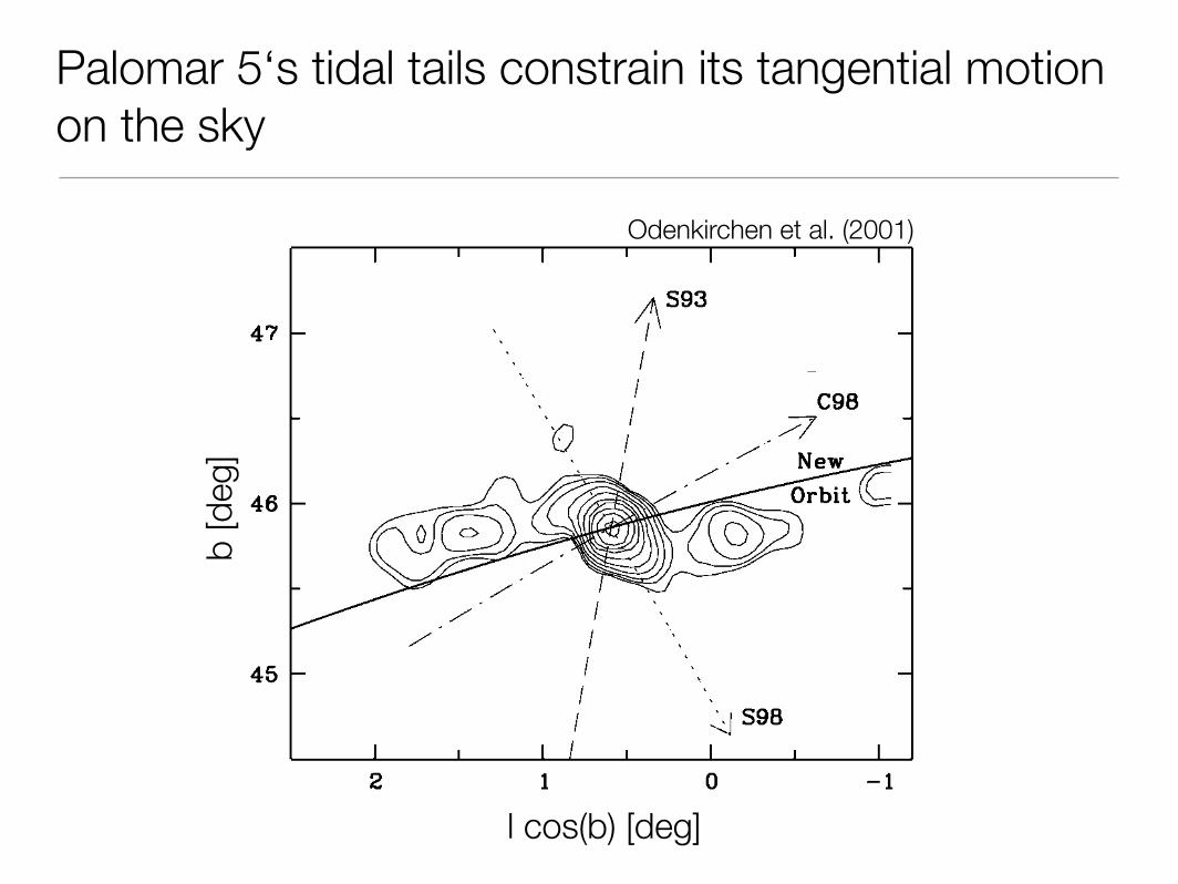
Palomar 5‘s tidal tails constrain its tangential motion on the sky
L168 TIDAL TAILS OF PAL 5 Vol. 548
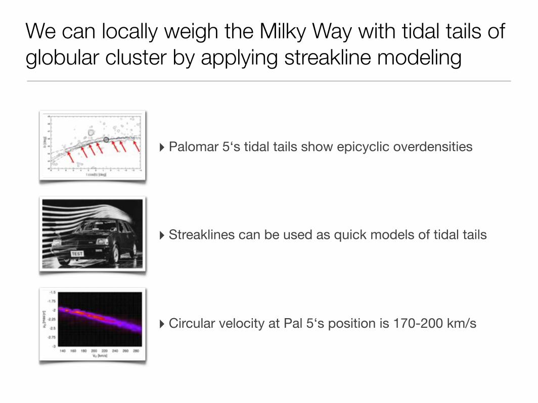
Fig. 3.—Contour plot of the surface density of cluster candidates in galacticcoordinates ( ) overlaid with different orbital paths of the cluster ac-l cos b, bcording to different determinations of its absolute proper motion: S93, S98,and C98. The solid line presents our improved estimate of the orbit based onthe geometry and orientation of the tidal tails (fixing the direction of tangentialmotion) and the proper motions by C98 and by S98 (estimating the tangentialvelocity).
i.e., in the direction to the galactic center and anticenter. Dueto differential galactic rotation, their trajectories then bendaround and continue approximately parallel to the orbit of thecluster. The appearance of clumps in the tails is also supportedby numerical simulations. They can be caused either by theenhanced release of particles after strong shock events or bycaustics of the trajectories in phase space.
3.2. The Role of Contaminants
In view of the striking resemblance of the detected structuresto the expected properties of tidal tails, significant contami-nation by clustered background objects seems a priori unlikely.Nevertheless, we checked this point by analyzing the densityand colors of non-pointlike SDSS sources around Pal 5 thatby their shape are classified as galaxies. Their spatial distri-bution is clumped and reveals known galaxy clusters like Abell2050 and 2035. However, most of these sources do not fallinto the color-magnitude window for members of Pal 5. If ourselection criteria for Pal 5 members are applied to the galaxysample, the surface density of galaxies drops to the level of0.3–0.6 of the field background density of the stellar sample.Moreover, the pattern of density variations in the galaxy sampledoes not correlate with the location of the tidal tails. Therefore,objects like those in the galaxy sample are not likely to causesignificant disturbances in the stellar sample. The only re-maining contaminants are compact galaxies with bluer colorsthat may not be well represented in the sample of known gal-axies. We believe that such objects have mostly been eliminatedby our color cut u*! mag. Finally, fluctuations in stel-!g " 0.4lar surface density due to variable interstellar absorption canbe ruled out because the mean level of absorption in the regionaround Pal 5 is low and because there is no hint for strongvariations (values of EB!V in the maps of Schlegel et al. 1998range between 0.05 and 0.07 mag).
3.3. Implications for and from the Cluster’s Orbit
The orientation of the tails provides unique information onthe direction of the cluster’s tangential motion since it is knownthat the leading and trailing parts must fit in with the inner andouter sides of the local orbit, respectively. Figure 3 reveals thatthe tails stretch out in the direction of constant b and that thetangential motion is very likely westward (prograde rotation).The absolute proper motions by Schweitzer, Cudworth, & Ma-jewski (1993, hereafter S93) and S98 yield very different pre-dictions for the local orbit, although at least the sense of rotationis in agreement. The proper motion given by K. Cudworth (1998,hereafter C98, unpublished revision of the work by S93, reportedin S98 and by private communication) yields a local orbit thatlies closer to the tails. From the observed orientation of the tails,we estimate that the tangential velocity vector points#15! northof the line of constant b. In order to meet this constraint,the proper motion needs to be modified by not more than0.4 mas yr with respect to C98’s values. We thus!1
adopt mas yr for the cluster’s!1m cos b, m p !0.93, " 0.25l b
proper motion in the galactic rest frame. With these values, weobtain an orbit (using the galactic potential of Allen & Santillan1991) with apo- and perigalactic distances of 19.0 and 7.0 kpc,respectively, and with disk passages at !137, !292, and!472 Myr taking place at Galactocentric radii of 9.4, 18.4, and8.3 kpc, respectively. Similar orbits are obtained with the moredetailed galactic potentials of Dehnen & Binney (1998). We tendto believe that the observed overdensities close to the cluster
result from the latest disk passage, while the clumps in the tailsat distances of #0!.8 from the cluster might be associated withthe earlier passage through the inner disk about 470 Myr ago.This, however, has to be investigated more thoroughly withN-body simulations. The next passage through the galactic diskpredicted by our model orbit will be in 113 Myr and will happenclose to perigalacticon. If true, this will again produce a strongtidal shock that may eventually dissolve the cluster completely.
3.4. Outlook
The SDSS will eventually cover a much larger region aroundPal 5 than currently available. Larger area coverage will enableus to constrain the orbit and mass loss more tightly. We canfurther constrain our model orbit by obtaining radial velocitiesof stars in the tails. We predict a local radial velocity gradientof 5.7 km s deg , i.e., an #9 km s difference between the!1 !1 !1
radial velocities of stars in the two tidal tail clumps. SincePal 5 contains very few luminous red giants, even fewer areexpected in its tails; thus, kinematic studies will have to con-centrate on fainter stars requiring large telescopes.
The Sloan Digital Sky Survey10 is a joint project of theUniversity of Chicago, Fermilab, the Institute for AdvancedStudy, the Japan Participation Group, Johns Hopkins Univer-sity, the Max Planck Institute for Astronomy, New MexicoState University, Princeton University, the US Naval Obser-vatory, and the University of Washington. The Apache PointObservatory, site of the SDSS telescopes, is operated by theAstrophysical Research Consortium. Funding for the projecthas been provided by the Alfred P. Sloan Foundation, the SDSSmember institutions, the National Aeronautics and Space Ad-ministration, the National Science Foundation, the US De-partment of Energy, Monbusho, and the Max Planck Society.
10 The SDSS Web site is located at http://www.sdss.org.
Odenkirchen et al. (2001)
l cos(b) [deg]
b [d
eg]
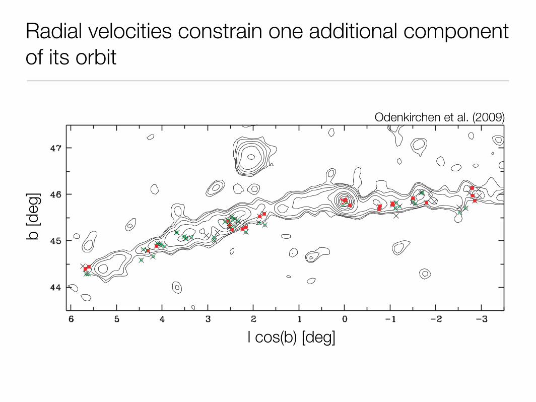
Radial velocities constrain one additional component of its orbit
3380 ODENKIRCHEN ET AL. Vol. 137
Figure 2. Position of the target stars (crosses) with respect to the tidal tails of Pal 5. The cluster and its tails are shown by isopleths of color–magnitude-selected starcounts (map taken from Paper III). The coordinates of the plot are galactic longitude and latitude. The meaning of the symbols is the same as in Figure 1. The plot alsoincludes the targets from Paper II (!l cos b ! 0.0, inside the cluster Pal 5).(A color version of this figure is available in the online journal.)
the advantage of providing five independent velocity measure-ments of approximately equal weight, from which one can drawa solid estimate of the accuracy of the results. The rms devi-ations of the individual measurements from their mean are inthe range 0.1–1.4 km s"1, depending on the quality of the spec-tra. The velocity corrections, which are needed to transform themeasured relative velocities into heliocentric absolute veloci-ties, were calculated with the IRAF routine RVCORRECT.
For the two standards we adopted the heliocentric veloc-ities given by Udry et al. (1999). In Paper III these valueswere found to be mutually consistent within a difference of0.14 km s"1. Our new measurements confirm this result. Wefind that the absolute velocities derived with the two differentstandard stars agree within a mean difference of 0.16 km s"1 andan rms dispersion of 0.10 km s"1. This shows that there is no sys-tematic difference other than the small difference between thestandard stars themselves and that the individual deviations arealso small. We adopt the average of the velocities obtained withthe two standards as the best estimate of the heliocentric velocityof each target. The repeated observation of one of the targets in2002 and 2003 yields velocities of "56.75 and "56.79 km s"1,respectively. This demonstrates that the results from period 1and period 2 are highly consistent. Because of these accuracychecks we are confident that there are no substantial systematicerrors in our measurements.
2.2. Medium-Resolution Spectroscopy
During the second observing period in 2003 we had the op-portunity to collect simultaneously medium-resolution spectrausing GIRAFFE. We thus obtained 174 spectra for additionaltargets along the RGB of Pal 5 in the same fields down to mag-nitude 19.5 in i, covering the wavelength range from 5051 to5831 Å at a nominal mean resolving power of R = 6000. Un-fortunately, the majority of these spectra suffered from too lowsignal-to-noise. Moreover, even those targets for which a radialvelocity could be derived, turned out to contain very few po-tential members of Pal 5, which were not distinguishable fromnonmembers. Therefore the medium-resolution spectra were notuseful for our project. They will hence not be discussed here anyfurther.
3. ANALYSIS OF THE KINEMATICS
3.1. Tidal Tail Membership
The UVES spectra provide not only precise radial velocitiesof the targets but also information on their stellar type. Asshown in Paper III, the line width of the Mg b triplet featurearound 5180 Å is a good indicator of the luminosity of thestar, allowing us to distinguish dwarfs (broad Mg b lines)from giants (narrow Mg b lines). This diagnostic permits us toclean the sample from foreground dwarf stars, which otherwisecould affect our attempt to trace the kinematics of the tidaldebris. Visual inspection of the spectra shows that despitephotometric preselection of the targets along the locus of Pal5’s giant branch only 21 of the targets are definitely giantswhereas 40 targets turned out to be dwarfs. For the remaining13 target stars the stellar type remains unclear because thesignal-to-noise ratio of the spectra is insufficient for a definiteclassification.
The dwarfs can immediately be discarded as members ofPal 5’s debris. The giants are plausible members, but it hasto be clarified whether they are really part of the debris orelse unrelated intervening halo stars. In Figures 1 and 2 thegiants, dwarfs, and ambiguous cases among our spectroscopictargets are shown by different plot symbols. It can be seenthat the brightest stars of the sample are all dwarfs, i.e., inthe tails of Pal 5 we do not find any giants with magnitudessimilar to those of the brightest red giants inside the cluster.At fainter magnitudes, however, the number of giants foundin the tails is comparable to the number of giants found inthe cluster. Thus the lack of brighter giants outside the clusterreveals a true photometric difference between the potentialdebris stars and the stellar population in the cluster (see alsoKoch et al. 2004). On the other hand, we observe that amongstars with i > 17.0 the spectroscopically observed giants tendto be concentrated toward the RGB of the cluster while thedwarfs cover the stripe between the border lines of photometricselection rather homogeneously. This is an important factbecause it suggests that the giants are not a random sample andindeed comprise of members of the tidal stream of the cluster.However, Figure 1 alone does not provide sufficiently strong
Odenkirchen et al. (2009)
l cos(b) [deg]
b [d
eg]
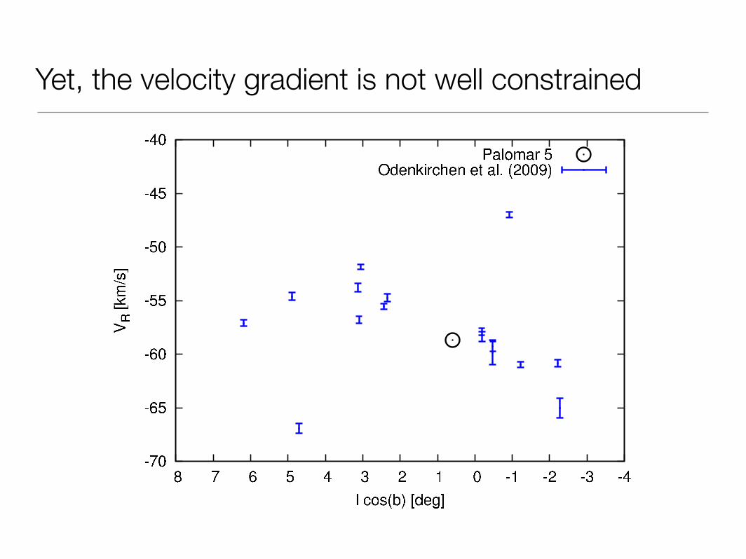
Yet, the velocity gradient is not well constrained
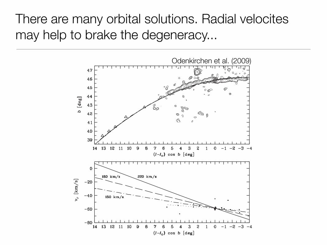
There are many orbital solutions. Radial velocites may help to brake the degeneracy...
No. 2, 2009 KINEMATICS OF TIDAL DEBRIS OF PAL5 3385
Figure 7. Analogous plot to Figure 6, but comparing orbits in halo potentials with different circular velocity vc . Solid line: orbit for vc = 220 km s!1 (same as inFigure 6). Dashed line: orbit for vc = 180 km s!1. Dashed-dotted line: orbit for vc = 150 km s!1. The tangential velocity vt of the cluster was adapted such that thethree orbits fit the location of the tidal debris on the sky equally well (see upper panel). Only for an implausibly low value of vc (see e.g., Xue et al. 2008) could theobserved velocities come close to the predictions for particles that lie exactly on the orbit.
in a potential with vc = 180 km s!1 (vt = 82 km s!1) and vc =150 km s!1 (vt = 69 km s!1), respectively. In projection on thesky these orbits are locally indistinguishable (see upper panel ofFigure 7), hence they fit the location of the tidal debris on the skyequally well. The kinematics, however, are different. The radialvelocity gradient becomes smaller as the circular velocity of thepotential decreases (see lower panel of Figure 7). Together withthe observations this suggests that the circular velocity in theGalactic halo is smaller than in the solar neighborhood.
However, in the case of vc = 180 km s!1 the radial velocitygradient of the orbit is 3.1 km s!1 deg!1 and hence stillconsiderably different from the observations. In order to bringthe velocity gradient down to the level of 1 km s!1 deg!1 oneneeds to decrease vc below 150 km s!1. Such a low circularvelocity would be quite extreme and difficult to reconcile withother data on the rotation curve of the outer Galaxy (e.g., Xueet al. 2008). Instead, it seems that variations in the Galacticpotential can at best contribute part of the solution and thatother factors also play a significant role.
4.2. Pal 5’s Distance
In contrast to the cluster’s position on the sky and its radialvelocity, which are both accurately known, the distance of thecluster is currently not known with high accuracy. The adopteddistance estimate of 23.2 kpc is derived from photometry ofits horizontal branch stars (providing a distance modulus of16.82 mag, Harris 1996). Taking into account photometric er-rors and uncertainties in the determination of the absolute mag-nitude of the horizontal branch the distance modulus probablyhas an uncertainty of about 0.2 mag. Hence an error of 10% inthe distance is likely.
Figure 8. Same as in Figure 6, but testing orbits with different distances of thecluster from the observer. Solid line: orbit for d = 23.2 kpc (same as in Figure 6).Dashed line: orbit for d = 21.2 kpc. Dashed-dotted line: orbit for d = 19.2 kpc.Again, the three orbits have identical projected paths on the sky (see upper panel).
In Figure 8 we compare orbits for three different distances,one with the standard d = 23.2 kpc (solid line, same as inFigures 6 and 7), one with d being 2 kpc smaller (long-dashedline), and one with d being 4 kpc smaller (dashed-dotted line).These orbits are derived using the standard potential with vc =220 km s!1. Again, the tangential velocity of the cluster has been
Odenkirchen et al. (2009)
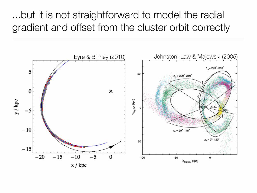
...but it is not straightforward to model the radial gradient and offset from the cluster orbit correctly
Eyre & Binney (2010)
!!
"20 "15 "10 "5 0
"15
"10
"5
0
5
x ! kpc
y!kpc
Johnston, Law & Majewski (2005)
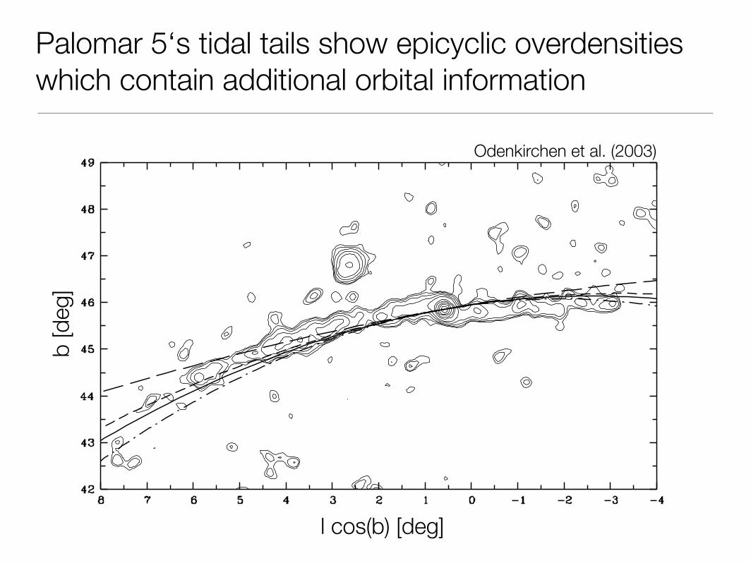
Palomar 5‘s tidal tails show epicyclic overdensities which contain additional orbital information
to the Galactic center, that is, those points where a force bal-ance between the internal field of the cluster and the externaltidal field exists. They are likely to pass these points withsmall relative velocity because the internal velocity disper-sion in the cluster is low, in particular in low-mass clusterssuch as Pal 5 (!los < 0.7 km s!1; Paper II). Subsequently, thedebris is decoupled from the cluster and behaves like aswarm of test particles that are radially o!set from the clus-ter and released with almost the same Galactocentric veloc-ity vector as the cluster. In the framework of the abovemodel and the ideal case of zero velocity dispersion, thismeans that the cluster and its debris are on confocal orbitsthat are equal up to radial scaling but have di!erent angularvelocities and thus exhibit azimuthal shear.
If the separation "’ between the azimuth angles of theshifted and the unshifted particle (i.e., between a debris starand the cluster) is small, the relation between "’ and thetime Dt since the release of the shifted particle can beexpressed in a simple formula. Provided that "’ is smallenough to ensure that the Galactocentric distance #R alongthe orbit of the shifted particle, and hence its angularvelocity, which is L/#R2, can be considered as beingapproximately constant over "’, it follows that
"’ " L
#R2"t # #! 1
#Dt
L
R2: $7%
Here "t means the time lag that corresponds to "’, forwhich equation (6) yields "t = (# ! 1)Dt. Note thatequation (7) is independent of the value of the circularvelocity vc of the potential. The relation shown inequation (7) is very useful because it provides a key forestimating the mass-loss rate of the cluster (see x 6).
5.2. Local Orbit and Tangential Velocity
We now describe what observational constraints we haveon the cluster’s local orbit, that is, its orbit near the presentposition of the cluster and the location of its tails. Adoptingd = 23.2 kpc (Harris 1996) for the heliocentric distance ofPal 5 and R& = 8.0 kpc for the distance of the Sun from theGalactic center, we derive the position of Pal 5 in the Galaxyas (x, y, z) = (8.2, 0.2, 16.6) kpc. Here x, y, and z denoteright-handed Galactocentric Cartesian coordinates, with ybeing parallel to the Galactic rotation of the local standardof rest and z pointing in the direction of the northern Galac-tic pole. In other words, the Sun has coordinates(!8.0, 0.0, 0.0) in this system. From the above position ofPal 5 it follows that the inclination between the line of sightand the orbital plane of the cluster must be '18(. On theother hand, our view of the orbital plane cannot be entirelyedge-on, because Figure 3 clearly shows the S-shapedbending of the tidal debris near the cluster. This featureobviously reflects the opposite radial o!sets between thetwo tails and the cluster. Considering the orientation of thisS feature and the perspective of the observer, we infer thatthe orbit of the cluster (in projection on the plane of the sky)must be located east of the northern tail and west of thesouthern tail (referring to the equatorial coordinate systemused in Fig. 3).
The simple model from x 5.1 tells us that the tidal debrisshould be on similar orbits as the cluster if velocitydi!erences can be neglected. Taking into account the localsymmetry of the tidal field, the limited range in azimuthangle ’ covered by the observations, and the relatively small
angle between the orbital plane and the line of sight, onethus expects the o!sets between the tails and the orbit of thecluster in projection on the tangential plane of the observerto be constant and of equal size on both sides of the cluster.An additional argument for this assumption is that the tailsshow a constant width, that is, the projection does notreveal that they become wider as a function of angular dis-tance from the cluster. If the mean (projected) separationbetween the tidal debris and the orbit of the cluster wereincreasing with angular distance from the cluster, one wouldexpect to see the tails become wider, which is not the case.Therefore we continue the analysis under the assumptionthat the cluster’s projected orbit runs parallel to the twotails.
First of all, this sets a tight constraint on the direction ofthe cluster’s velocity vector in the tangential plane. The tailsimply that the tangential motion of the cluster has a positionangle of 231( ) 2( with respect to the direction pointing tothe northern equatorial pole, and 280( ) 2( with respectto Galactic north (see Fig. 8). The orientation of this angle(i.e., P.A. = 280( and not P.A. = 100() follows when takinginto account the direction to the Galactic center. Figure 9shows the surface density map of the tails on a grid ofGalactic celestial coordinates (l cos b, b), where l is Galacticlongitude and b Galactic latitude. Since the Galactic center(l = 0(, b = 0() lies to the bottom of this plot, the tail thatpoints to the right (also called the southern tail), must be theone at smaller Galactocentric distance, which is thus lead-ing, and the tail that points to the left (also called thenorthern tail) be the more distant one, which trails behind.This means that the cluster is in prograde rotation aboutthe Galaxy, in agreement with indications from di!erentmeasurements of its absolute proper motion (Schweitzer,Cudworth, & Majewski 1993; Scholz et al. 1998; K. M.Cudworth 1998, unpublished, cited in Dinescu, Girard, &van Altena 1999).
Next we consider whether the observed part of the streamis long enough to see a deviation from straight-line motion.
Fig. 9.—Tails and local Galactic orbit of Pal 5 plotted in Galacticcoordinates (l cos b, b). Projections of four di!erent orbits, all with tangenttoward position angle 280( at the center of the cluster, are overplotted onthe contour map of Fig. 3. Long-dashed line: Straight-line (i.e., unacceler-ated) motion. Solid line: Locally best-fitting orbit in a radial field ofconstant acceleration a = (220 km s!1)2/18.5 kpc. Here the cluster has atangential velocity of vt = 95 km s!1 (Galactic rest frame, but viewed fromthe position of the Sun). Dashed and dash-dotted lines: Orbits in the samefield, but with vt = 110 km s!1 and vt = 80 km s!1, respectively. Note that alogarithmic potential with circular velocity vc = 220 km s!1 instead of thea = const field yields projected local orbits that are practically identical tothose shown above.
No. 5, 2003 EXTENDED TAILS OF PAL 5 2395
Odenkirchen et al. (2003)
l cos(b) [deg]
b [d
eg]
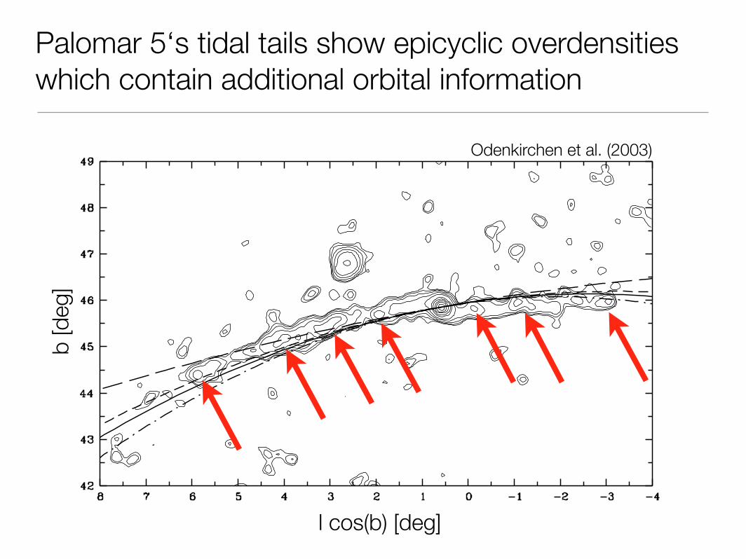
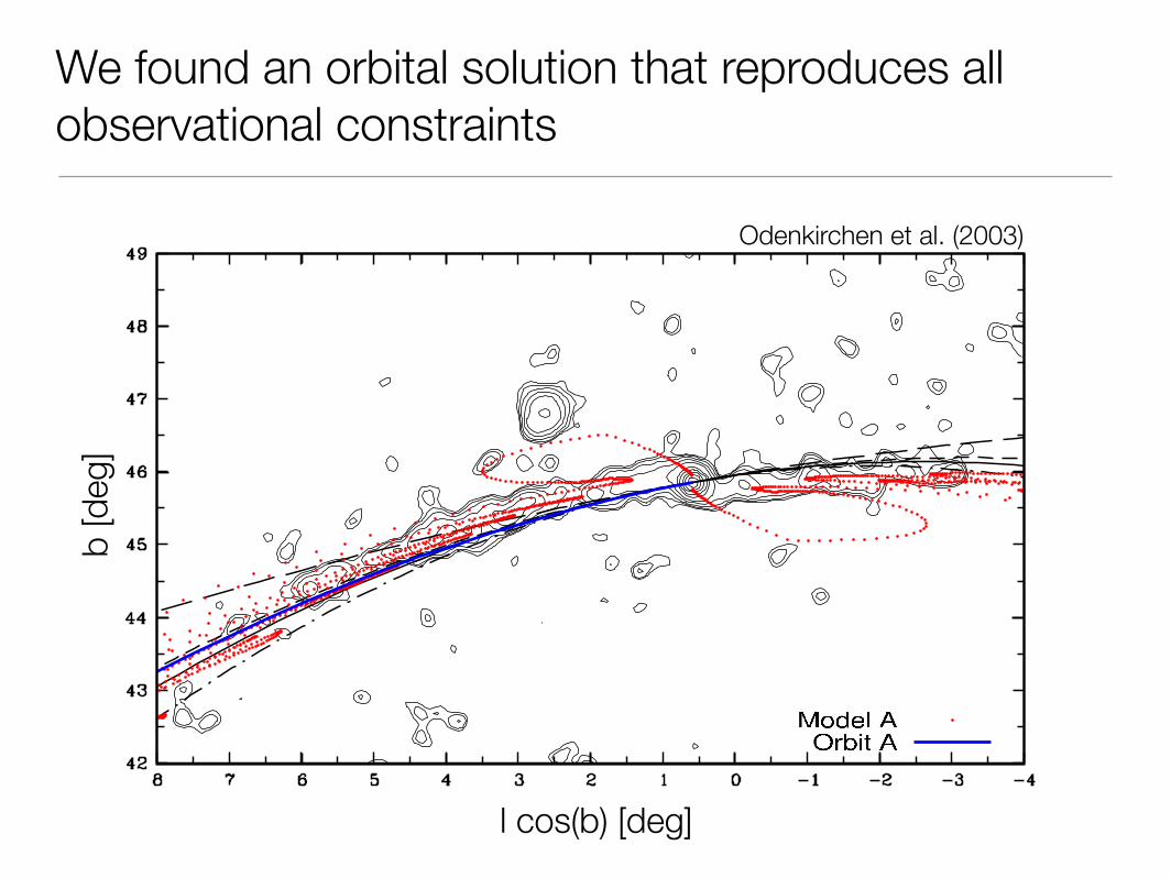
We found an orbital solution that reproduces all observational constraints
to the Galactic center, that is, those points where a force bal-ance between the internal field of the cluster and the externaltidal field exists. They are likely to pass these points withsmall relative velocity because the internal velocity disper-sion in the cluster is low, in particular in low-mass clusterssuch as Pal 5 (!los < 0.7 km s!1; Paper II). Subsequently, thedebris is decoupled from the cluster and behaves like aswarm of test particles that are radially o!set from the clus-ter and released with almost the same Galactocentric veloc-ity vector as the cluster. In the framework of the abovemodel and the ideal case of zero velocity dispersion, thismeans that the cluster and its debris are on confocal orbitsthat are equal up to radial scaling but have di!erent angularvelocities and thus exhibit azimuthal shear.
If the separation "’ between the azimuth angles of theshifted and the unshifted particle (i.e., between a debris starand the cluster) is small, the relation between "’ and thetime Dt since the release of the shifted particle can beexpressed in a simple formula. Provided that "’ is smallenough to ensure that the Galactocentric distance #R alongthe orbit of the shifted particle, and hence its angularvelocity, which is L/#R2, can be considered as beingapproximately constant over "’, it follows that
"’ " L
#R2"t # #! 1
#Dt
L
R2: $7%
Here "t means the time lag that corresponds to "’, forwhich equation (6) yields "t = (# ! 1)Dt. Note thatequation (7) is independent of the value of the circularvelocity vc of the potential. The relation shown inequation (7) is very useful because it provides a key forestimating the mass-loss rate of the cluster (see x 6).
5.2. Local Orbit and Tangential Velocity
We now describe what observational constraints we haveon the cluster’s local orbit, that is, its orbit near the presentposition of the cluster and the location of its tails. Adoptingd = 23.2 kpc (Harris 1996) for the heliocentric distance ofPal 5 and R& = 8.0 kpc for the distance of the Sun from theGalactic center, we derive the position of Pal 5 in the Galaxyas (x, y, z) = (8.2, 0.2, 16.6) kpc. Here x, y, and z denoteright-handed Galactocentric Cartesian coordinates, with ybeing parallel to the Galactic rotation of the local standardof rest and z pointing in the direction of the northern Galac-tic pole. In other words, the Sun has coordinates(!8.0, 0.0, 0.0) in this system. From the above position ofPal 5 it follows that the inclination between the line of sightand the orbital plane of the cluster must be '18(. On theother hand, our view of the orbital plane cannot be entirelyedge-on, because Figure 3 clearly shows the S-shapedbending of the tidal debris near the cluster. This featureobviously reflects the opposite radial o!sets between thetwo tails and the cluster. Considering the orientation of thisS feature and the perspective of the observer, we infer thatthe orbit of the cluster (in projection on the plane of the sky)must be located east of the northern tail and west of thesouthern tail (referring to the equatorial coordinate systemused in Fig. 3).
The simple model from x 5.1 tells us that the tidal debrisshould be on similar orbits as the cluster if velocitydi!erences can be neglected. Taking into account the localsymmetry of the tidal field, the limited range in azimuthangle ’ covered by the observations, and the relatively small
angle between the orbital plane and the line of sight, onethus expects the o!sets between the tails and the orbit of thecluster in projection on the tangential plane of the observerto be constant and of equal size on both sides of the cluster.An additional argument for this assumption is that the tailsshow a constant width, that is, the projection does notreveal that they become wider as a function of angular dis-tance from the cluster. If the mean (projected) separationbetween the tidal debris and the orbit of the cluster wereincreasing with angular distance from the cluster, one wouldexpect to see the tails become wider, which is not the case.Therefore we continue the analysis under the assumptionthat the cluster’s projected orbit runs parallel to the twotails.
First of all, this sets a tight constraint on the direction ofthe cluster’s velocity vector in the tangential plane. The tailsimply that the tangential motion of the cluster has a positionangle of 231( ) 2( with respect to the direction pointing tothe northern equatorial pole, and 280( ) 2( with respectto Galactic north (see Fig. 8). The orientation of this angle(i.e., P.A. = 280( and not P.A. = 100() follows when takinginto account the direction to the Galactic center. Figure 9shows the surface density map of the tails on a grid ofGalactic celestial coordinates (l cos b, b), where l is Galacticlongitude and b Galactic latitude. Since the Galactic center(l = 0(, b = 0() lies to the bottom of this plot, the tail thatpoints to the right (also called the southern tail), must be theone at smaller Galactocentric distance, which is thus lead-ing, and the tail that points to the left (also called thenorthern tail) be the more distant one, which trails behind.This means that the cluster is in prograde rotation aboutthe Galaxy, in agreement with indications from di!erentmeasurements of its absolute proper motion (Schweitzer,Cudworth, & Majewski 1993; Scholz et al. 1998; K. M.Cudworth 1998, unpublished, cited in Dinescu, Girard, &van Altena 1999).
Next we consider whether the observed part of the streamis long enough to see a deviation from straight-line motion.
Fig. 9.—Tails and local Galactic orbit of Pal 5 plotted in Galacticcoordinates (l cos b, b). Projections of four di!erent orbits, all with tangenttoward position angle 280( at the center of the cluster, are overplotted onthe contour map of Fig. 3. Long-dashed line: Straight-line (i.e., unacceler-ated) motion. Solid line: Locally best-fitting orbit in a radial field ofconstant acceleration a = (220 km s!1)2/18.5 kpc. Here the cluster has atangential velocity of vt = 95 km s!1 (Galactic rest frame, but viewed fromthe position of the Sun). Dashed and dash-dotted lines: Orbits in the samefield, but with vt = 110 km s!1 and vt = 80 km s!1, respectively. Note that alogarithmic potential with circular velocity vc = 220 km s!1 instead of thea = const field yields projected local orbits that are practically identical tothose shown above.
No. 5, 2003 EXTENDED TAILS OF PAL 5 2395
Odenkirchen et al. (2003)
l cos(b) [deg]
b [d
eg]
How can we weigh the Milky Way using tidal tails of globular clusters?
The tidal tails of Palomar 5
Streaklines - a concept from continuum mechanics
Extracting Palomar 5‘s orbit using streaklines
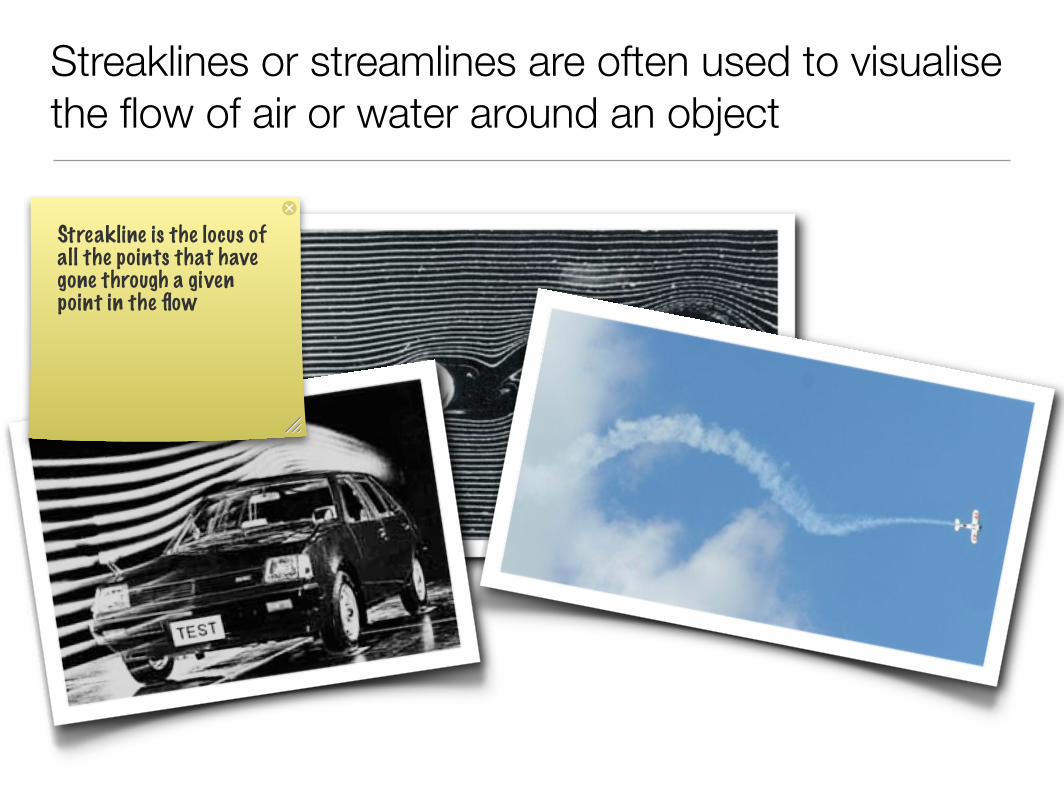
Streaklines or streamlines are often used to visualise the flow of air or water around an object
Streakline is the locus of all the points that have gone through a given point in the flow
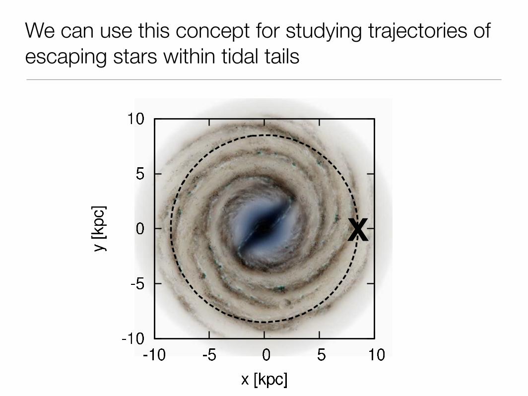
We can use this concept for studying trajectories of escaping stars within tidal tails
X
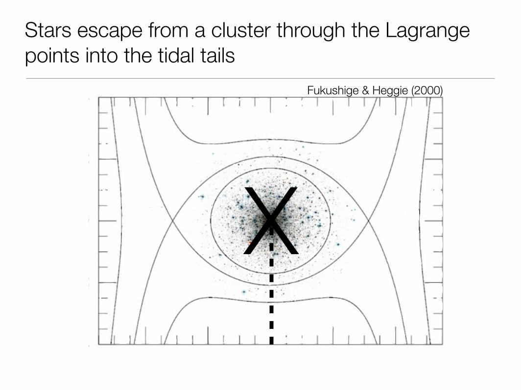
Stars escape from a cluster through the Lagrange points into the tidal tails
X
Fukushige & Heggie (2000)
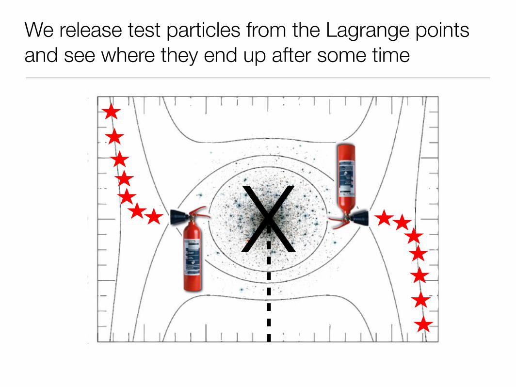
We release test particles from the Lagrange points and see where they end up after some time
X
Fukushige & Heggie (2000)
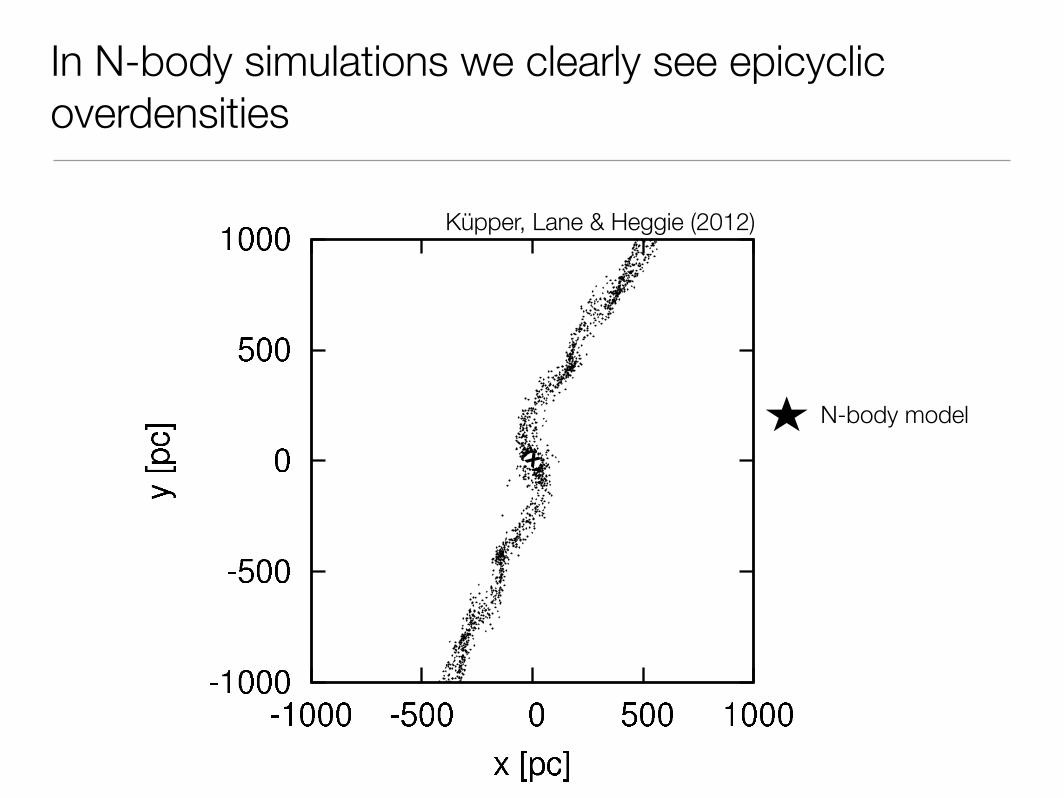
In N-body simulations we clearly see epicyclic overdensities
Küpper, Lane & Heggie (2012)
x
N-body model
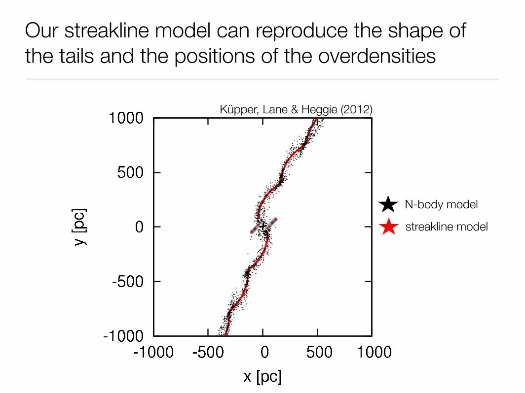
Our streakline model can reproduce the shape of the tails and the positions of the overdensities
streakline model
Küpper, Lane & Heggie (2012)
x
N-body model
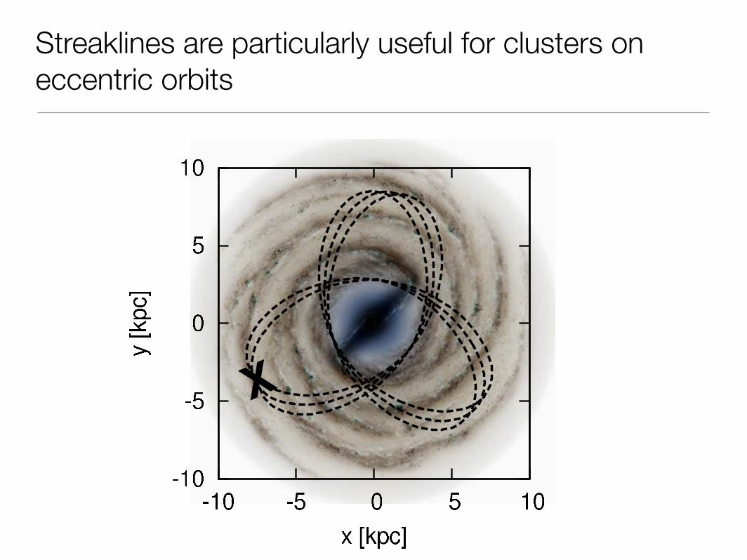
Streaklines are particularly useful for clusters on eccentric orbits
X
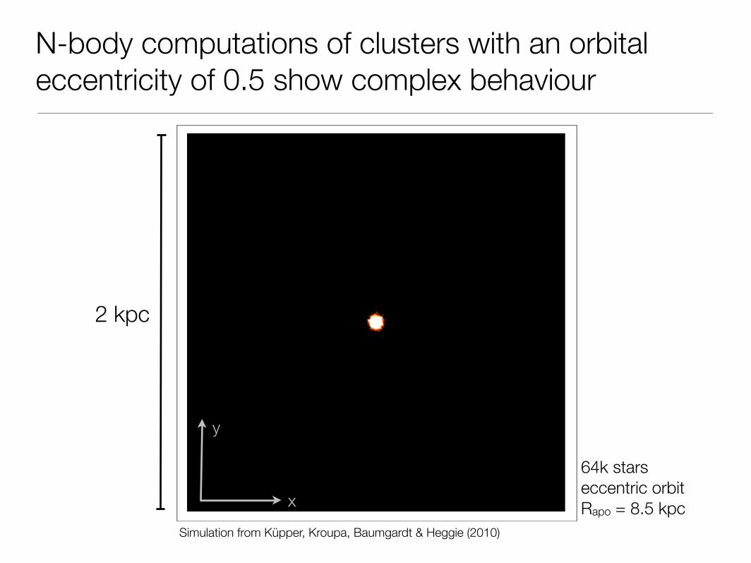
N-body computations of clusters with an orbital eccentricity of 0.5 show complex behaviour
x
y
x
z
Simulation from Küpper, Kroupa, Baumgardt & Heggie (2010)
64k starseccentric orbitRapo = 8.5 kpc
2 kpc
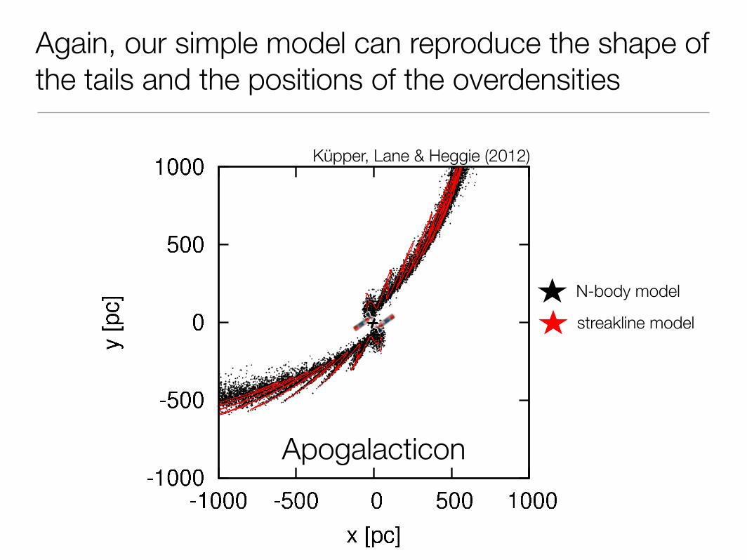
Again, our simple model can reproduce the shape of the tails and the positions of the overdensities
Apogalacticon
Küpper, Lane & Heggie (2012)
x streakline model
N-body model
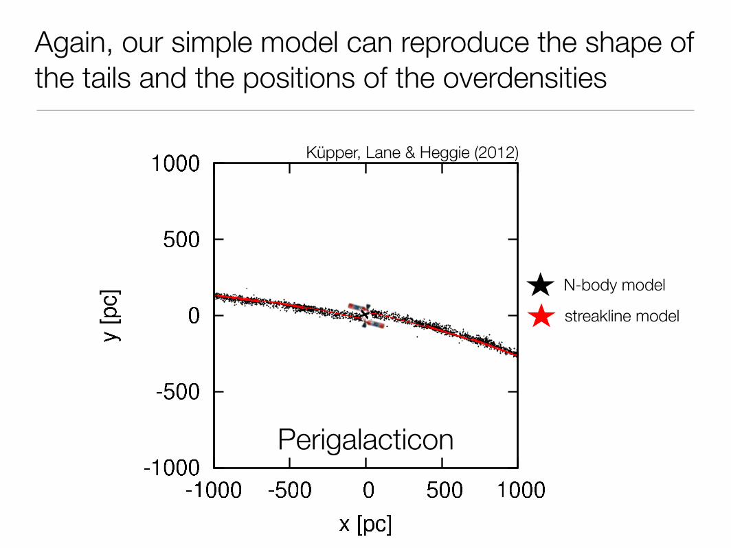
Again, our simple model can reproduce the shape of the tails and the positions of the overdensities
Perigalacticon
Küpper, Lane & Heggie (2012)
x
streakline model
N-body model
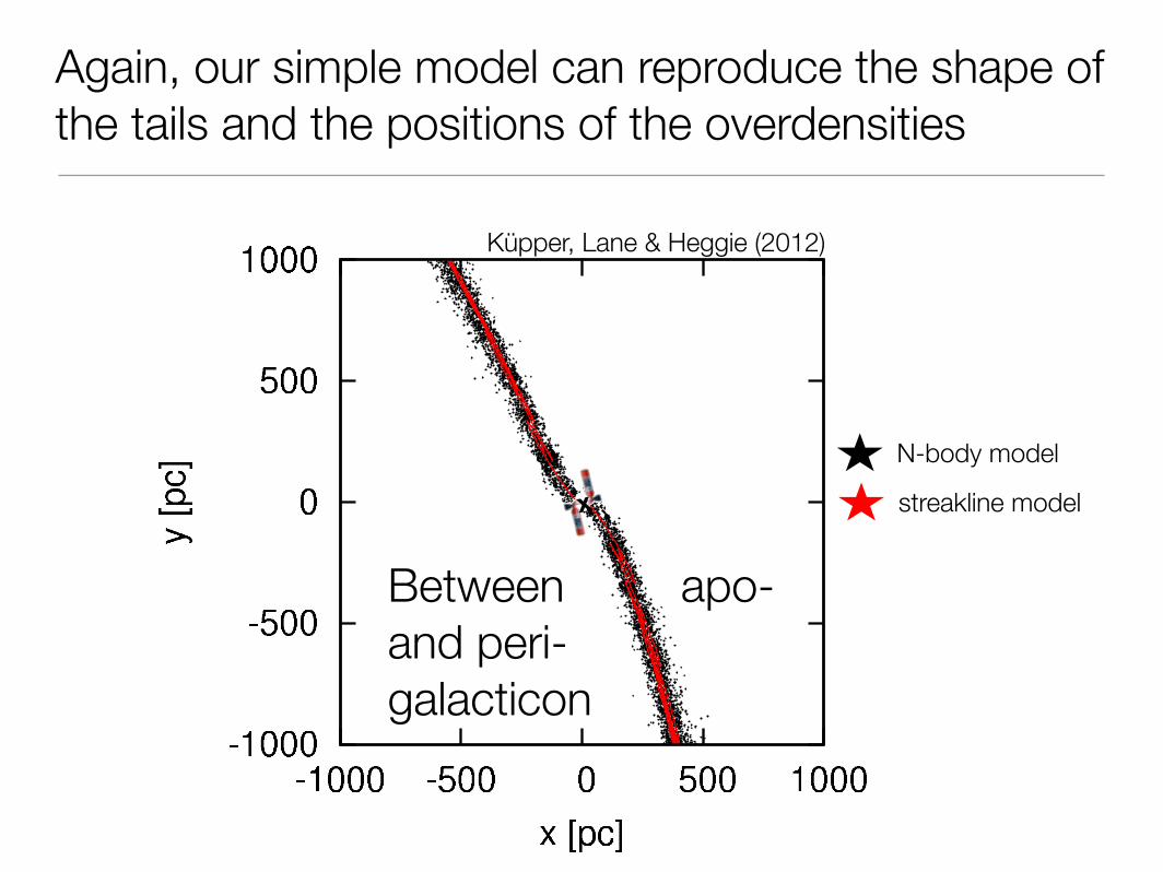
Again, our simple model can reproduce the shape of the tails and the positions of the overdensities
Between apo- and peri- galacticon
Küpper, Lane & Heggie (2012)
x streakline model
N-body model
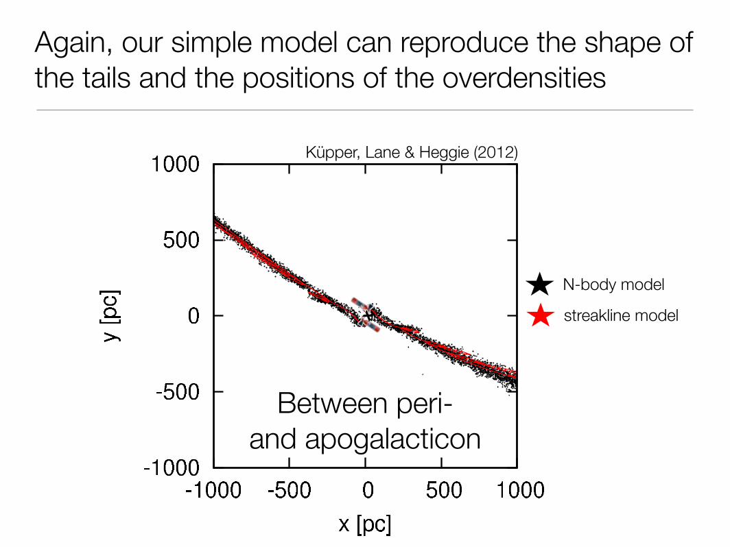
Again, our simple model can reproduce the shape of the tails and the positions of the overdensities
Between peri- and apogalacticon
Küpper, Lane & Heggie (2012)
x streakline model
N-body model
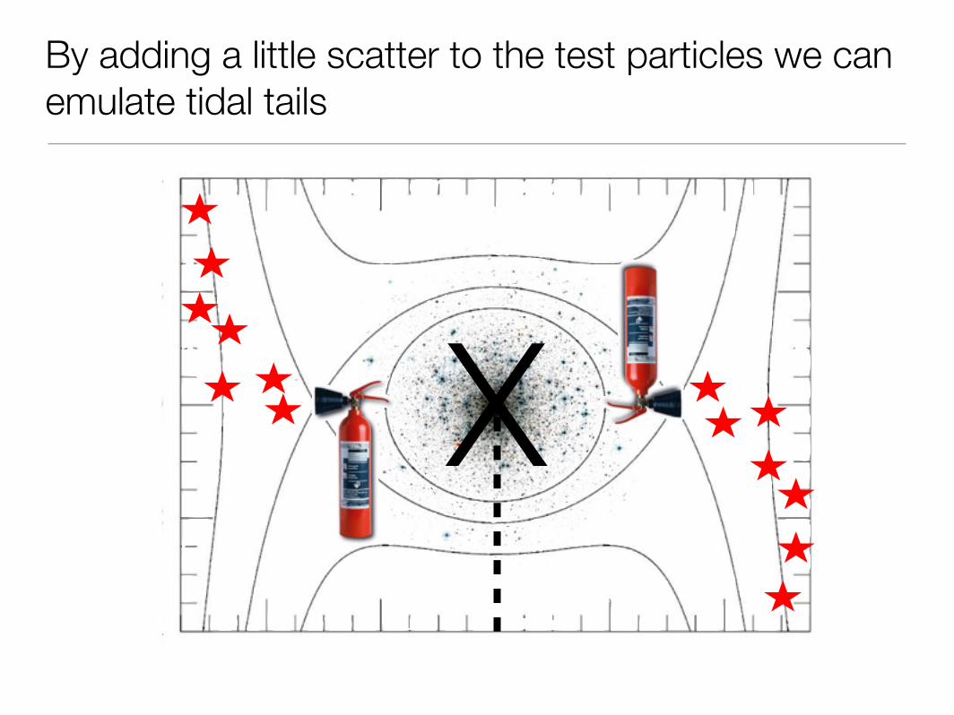
By adding a little scatter to the test particles we can emulate tidal tails
X
Fukushige & Heggie (2000)
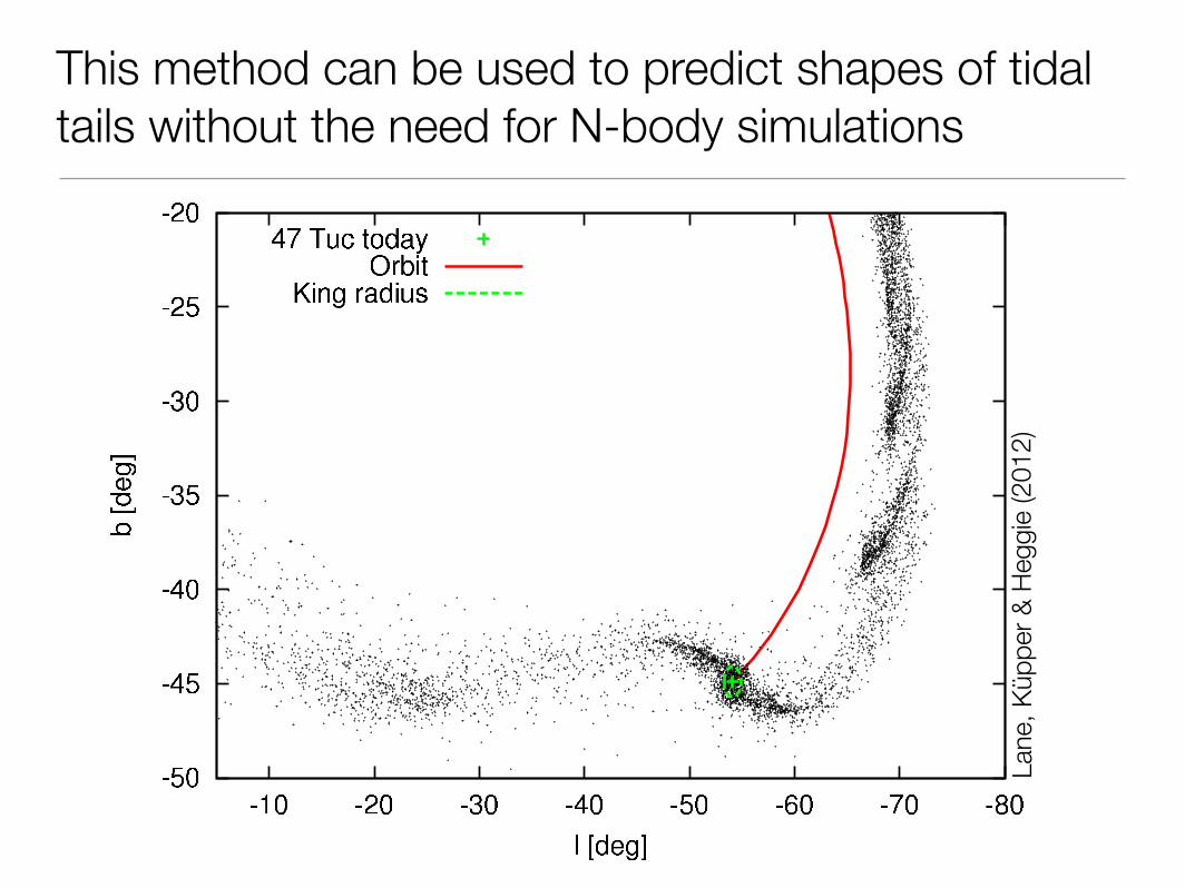
This method can be used to predict shapes of tidal tails without the need for N-body simulationsThe Tidal Tails of 47 Tucanae 5
Figure 3. The final timestep (present time) of the referencemodel is shown. The black points are test particles. Due to the
manner in which they were released from the cluster,
these particles can be considered streaklines, which al-
low for a simple visualisation of the positions, at the present
time, of stars which have escaped from 47 Tuc in the re-
cent past. These have been produced by releasing test particlesfrom the tidal radius of the cluster (see text). The solid red curveis the orbital path of the cluster. The current position of the clus-ter is marked by a green cross, and its King radius as derived fromits surface density profile (see Fig. 1) is given by the green dashedcurve. Escaped stars are slowest within the epicyclic loops, whichis where overdensities will be visible.
cluster. Therefore, we will first discuss a reference model,then we will vary single parameters to study the e!ect ofthe changes.
Table 1 describes the parameters we have chosen forour reference model. This reference cluster has a total finalmass of 1.0 ! 106 M! and loses one star every 0.075 Myr.Its proper motion is given by µ! = 5.64 mas yr"1 andµ" = "2.05 mas yr"1 and it has a Heliocentric distance of4.02 kpc. We run our simulations for 1000 Myr, finishing atthe present time. We have chosen 1000 Myr as this is longenough for the first, second and third order overdensities inthe tidal tails to become fully populated.
In Fig. 3 the streaklines of the above setup are shown.To produce these lines we released the test particles withexactly the angular velocity of the cluster from exactly theLagrange points (Eq. 4). The edge radius for this clustermass was found to be 158 pc, whereas the actual tidal ra-dius of the cluster varies between 111 pc at perigalacticonand 171 pc at apogalacticon. The epicyclic motion of thetest particles in the tails is obvious. The epicyclic loops arestrongly influenced and disturbed by the cluster mass.
In Fig. 4 the simulated tails of 47 Tuc are shown for twodi!erent sets of escape conditions. For the ‘warm’ escapeconditions (top panel), the escaping stars retain the angularvelocity of the cluster plus they obtain a random o!set invelocity drawn from a Gaussian distribution with a FWHMof 1 km s"1. Moreover, a Gaussian o!set with a FWHM of25% of the tidal radius has been added about the Lagrangepoints so that they do not all escape from a single pointon the edge of the cluster. For the ‘hot’ escape conditions(bottom panel in Fig. 4) we doubled the above fluctuations,i.e. a Gaussian velocity o!set with a FWHM of 2 km s"1
Figure 4. Same as Fig. 3, except with ‘warm’ (top panel) and‘hot’ (bottom panel) escape conditions of the test particles (blackpoints) as described in the text. Each test particle has been givena random spatial o!set and a velocity o!set at the moment ofescape. Because of these o!sets the test particles no longer liealong a smooth curve as in Fig. 3. The larger the spread in es-cape conditions, the lower the peak density within the epicyclicoverdensities, however, the locations of the overdensities are onlynegligibly a!ected.
and a Gaussian spatial o!set with FWHM of 50% of thetidal radius. However, from Kupper, Lane & Heggie (2012)it is obvious that the scatter in escape conditions is in factnot very large. Hence, the ‘hot’ escape conditions can beregarded as the ‘worst case scenario’.
We see that adding random fluctuations to the escapeconditions of the test particles increases the width of thetails and scatters their orbits about the ideal orbits shownin Fig. 3. The larger the scatter in escape conditions, thesmaller the peak density in the epicyclic overdensities. How-ever, the positions of the overdensities is not altered signifi-cantly.
Furthermore, we have produced several simulationsto test how the uncertainty in the input parameter val-ues a!ects the output of our model. For proper motion,we produce models with µ! = 4.23 mas yr"1 and µ! =7.05 mas yr"1 as well as with µ" = "1.54 mas yr"1 andµ" = "2.56 mas yr"1. For our decreased and increased massmodels we employ a cluster mass of 0.9 ! 106 M! and
Lane
, Küp
per
& H
eggi
e (2
012)
How can we weigh the Milky Way using tidal tails of globular clusters?
The tidal tails of Palomar 5
Streaklines - a concept from continuum mechanics
Extracting Palomar 5‘s orbit using streaklines
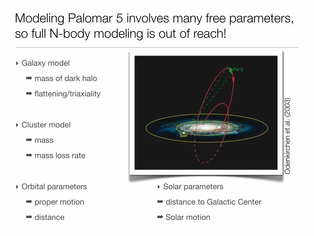
Modeling Palomar 5 involves many free parameters, so full N-body modeling is out of reach!
‣ Galaxy model
➡ mass of dark halo
➡ flattening/triaxiality
‣ Cluster model
➡ mass
➡ mass loss rate
‣ Orbital parameters
➡ proper motion
➡ distance
‣ Solar parameters
➡ distance to Galactic Center
➡ Solar motion
Ode
nkirc
hen
et a
l. (2
003)
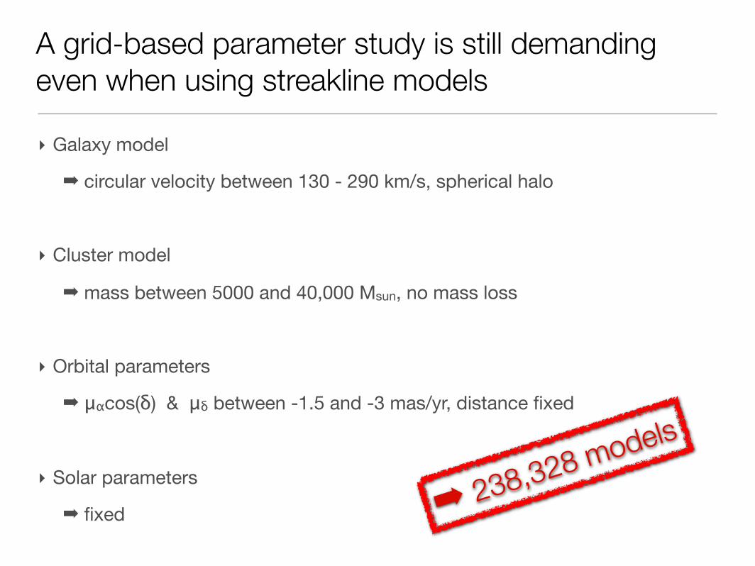
A grid-based parameter study is still demanding even when using streakline models
‣ Galaxy model
➡ circular velocity between 130 - 290 km/s, spherical halo
‣ Cluster model
➡ mass between 5000 and 40,000 Msun, no mass loss
‣ Orbital parameters
➡ μαcos(δ) & μδ between -1.5 and -3 mas/yr, distance fixed
‣ Solar parameters
➡ fixed ➡ 238,328 models
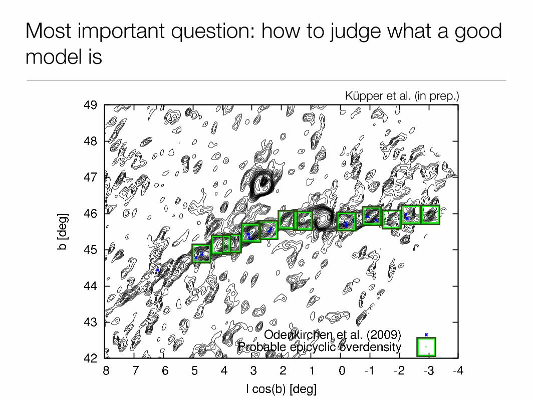
Most important question: how to judge what a good model is
Küpper et al. (in prep.)
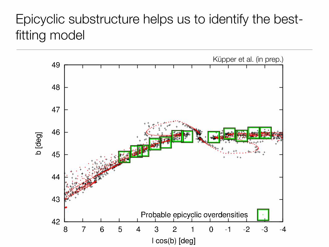
Epicyclic substructure helps us to identify the best-fitting model
Küpper et al. (in prep.)
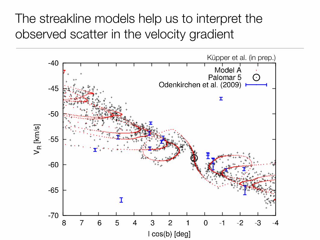
The streakline models help us to interpret the observed scatter in the velocity gradient
Küpper et al. (in prep.)
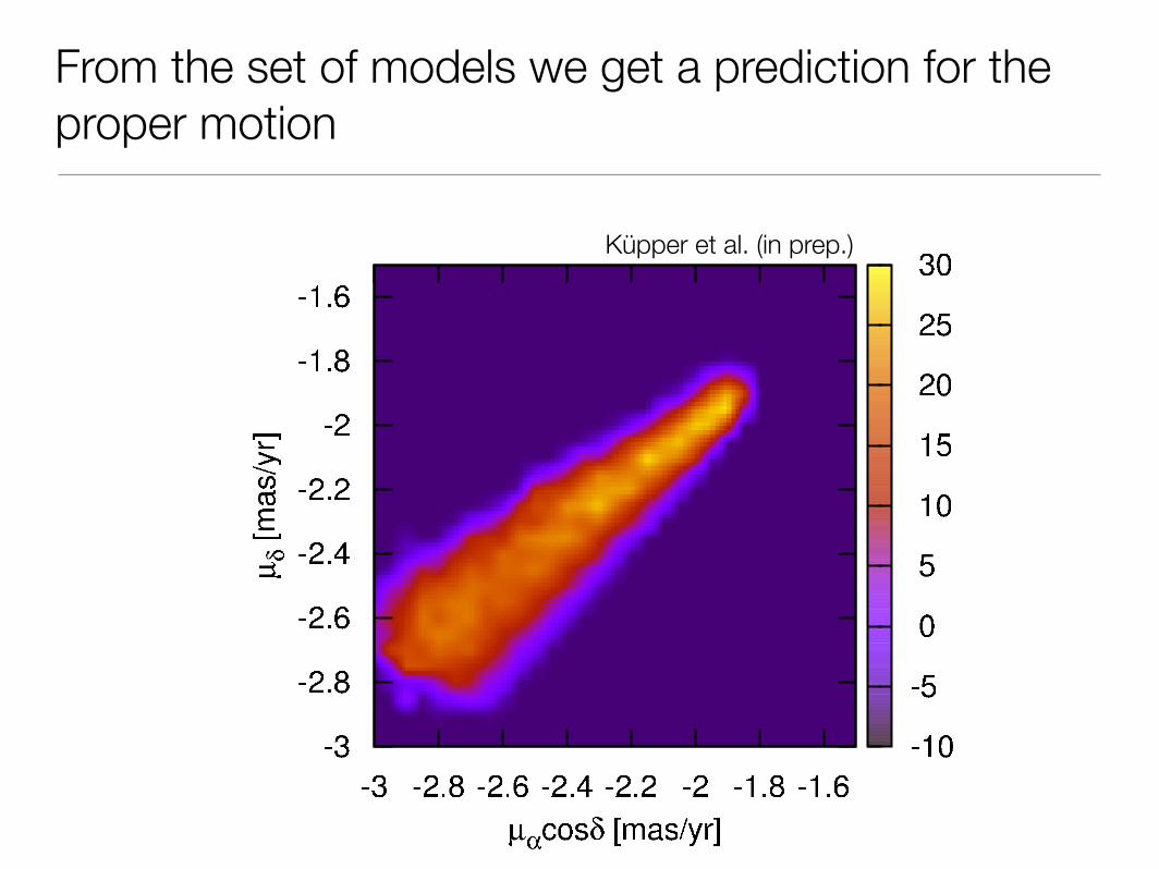
From the set of models we get a prediction for the proper motion
Küpper et al. (in prep.)
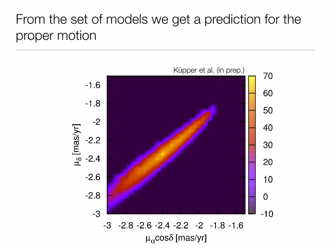
From the set of models we get a prediction for the proper motion
Küpper et al. (in prep.)
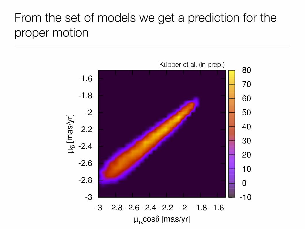
From the set of models we get a prediction for the proper motion
Küpper et al. (in prep.)
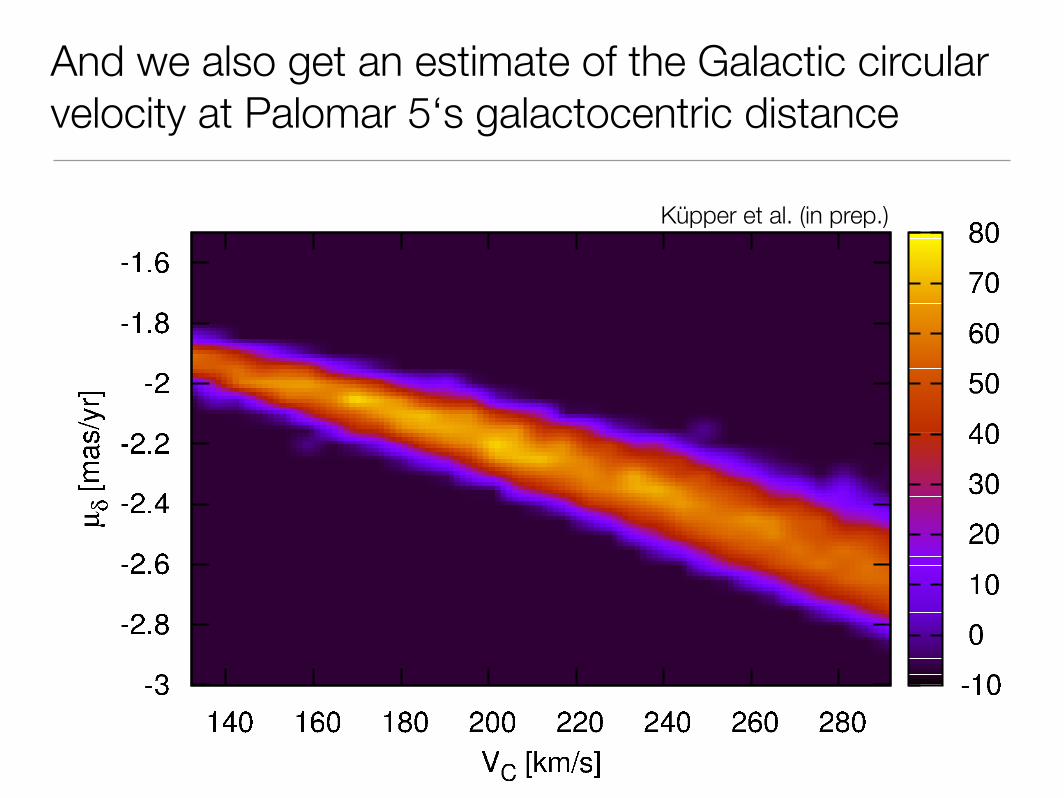
And we also get an estimate of the Galactic circular velocity at Palomar 5‘s galactocentric distance
Küpper et al. (in prep.)
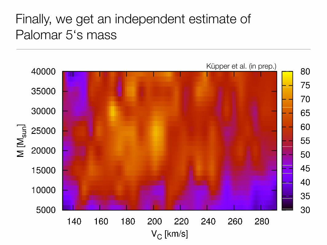
Finally, we get an independent estimate of Palomar 5‘s mass
Küpper et al. (in prep.)
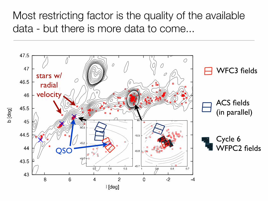
Most restricting factor is the quality of the available data - but there is more data to come...
QSO
stars w/radial
velocity
WFC3 fields
ACS fields (in parallel)
Cycle 6WFPC2 fields
11
Fig. 6.— The MilkyWay’s rotation curve in the range 4< R < 14kpc as inferred from our data for di!erent forms of the shape of therotation curve. At each R, the range in Vc(R) from 10,000 samplesof the PDF—assuming a power-law or cubic-polynomial model forthe shape of the rotation curve—is determined and the 68%, 95%,and 99% intervals are shown in varying shades of gray. For thecubic-polynomial model, we impose a prior that R0 < 9 kpc (seetext). For comparison, the squares show the rotation curve of M31from the compilation of Carignan et al. (2006).
V!,! = 242+5"17 km s"1 (for a power-law fit to the rota-
tion curve). In the latter fit, there is a strong correlationbetween Vc and V!,!; the di!erence between the two ismuch better constrained: V!,! ! Vc = 23.1+3.6
"0.5 km s"1.The marginalized PDF for V!,! ! Vc in FIG. 5 is well-described by V!,! ! Vc = 26± 3 km s"1. We discuss theconsequences of this solar motion in detail in § 5.3, butwe note here that the estimate of the angular motion ofthe Galactic center that we obtain from combining ourfits for V!,! and R0 is consistent with the proper motionof Sgr A# as measured by Reid & Brunthaler (2004): ourestimate is µSgr A! = 6.3+0.1
"0.7mas yr"1, compared to thedirect measurement of 6.379 ± 0.024mas yr"1. We dis-cuss the apparent discrepancy between our agreementwith the proper motion of Sgr A# and our low value forVc in § 5.3.The final block of parameters in TABLE 2 describe
the tracer population. The velocity dispersion that weinfer for the tracer stars is close to that expected foran old disk population: !R(R0) " 32.0+0.5
"3 km s"1 forthe flat-rotation-curve and power-law fits. The ratio ofthe tangential-to-radial velocity dispersions squared is0.69 < X2 < 1.0, with the best-fit value at the lower end
of this range. This value is higher than expected fromthe epicycle approximation for a flat or falling rotationcurve, which is X2 # 0.5. However, this expectationholds only for a cold disk, and corrections due to thetemperature of the old disk population always increaseX2 near R0 (Kuijken & Tremaine 1991): the Dehnendisk distribution functions of Equation (6) have X2 thatvaries spatially, and reaches approximately 0.65 near R0(Dehnen 1999). The best-fit value for R0/h" is approx-imately zero, with non-zero positive values ruled out bythe data: the 68% interval is !0.24 < R0/h" < 0.03.Thus, the radial-velocity dispersion does not drop expo-nentially with radius with a scale length between 2R0/3and R0; such a drop would be expected from previ-ous measurements of the radial dispersion as a func-tion of R (Lewis & Freeman 1989), or from the observedexponential decline of the vertical velocity dispersion(Bovy et al. 2012b) combined with the assumption ofconstant !z/!R. We have attempted fits with two popu-lations of stars with di!erent radial scale lengths (3 kpcand 5 or 6 kpc) and radial-velocity dispersions, but thesame radial-dispersion scale length. The best-fit R0/h"remains zero, such that it does not seem that we are see-ing a mix of multiple populations that conspire to forma flat !R profile.Even with the best-fit flat radial-dispersion profile, the
disk is stable over most of the range in R consideredhere. The Toomre Q parameter—Q = !R "/(3.36G")(Toomre 1964)—for a flat rotation curve is
Q = 1.72
!
!R
32 km s"1
" !
Vc
220 km s"1
"
!
R
8 kpc
""1 !
"
50M! pc"2
""1
.
(9)
This expression has Q > 1 down to 4.9 kpc and Q = 0.91at R = 4 kpc for a constant !R(R) and a surface den-sity " $ e"R/(3 kpc). Although the disk is marginallyunstable in our best-fit model, this conclusion dependsstrongly on the assumed radial scale length: for hR =3.25 kpc, Q > 1 everywhere at R > 4 kpc. The flat-ness of the inferred !R profile also depends on the as-sumed constancy of X2. Actual equilibrium axisymmet-ric disks, such as those having a Dehnen distributionfunction (Equation (6)), have a radially-dependent X2,with X2 at R = 4 kpc typically smaller than at R = 8 to16 kpc (Dehnen 1999, Figure 4). AtR = 4 kpc, which forthe present data sample is only reached for the l = 30$
line of sight, the line-of-sight velocity is entirely com-posed of the tangential-velocity component, such thatany decrease in X2 leads to an increase in !R to sustainthe same !!. Therefore, the true !R(R) profile presum-ably is falling with R, and the entire disk at R > 4 kpcshould be stable in our model.Full PDFs for all of the parameters of the basic models
discussed in this section are given in FIG. 5. It is clearthat with the exception of Vc and the derivative of therotation curve—# in the power-law model and dVc/dRin the linear model—there are no strong degeneraciesamong the parameters. Also included in this figure arethe results from fitting all but one of the 14 APOGEEfield for each field: these leave-one-out results show thatno single field drives the analysis for any of the parame-
In the solar neighbourhood we observe a circular velocity of 220 km/s
Bovy et al. (2012)
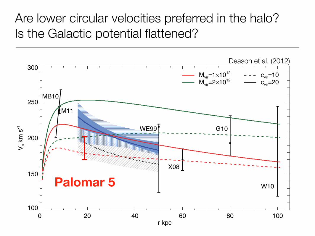
Are lower circular velocities preferred in the halo? Is the Galactic potential flattened?
L48 A. J. Deason et al.
Figure 4. The circular velocity profile of the Galaxy. The blue shaded region shows the 1! constraint found in this work for our favoured tracer density profileof DBE. The blue vertical and horizontal line filled regions indicate the additional uncertainty with systematic errors in the tracer density power-law indexof ±0.2 dex. The grey line filled region shows the profile when instead a spherical tracer density with power-law index 3.5 is used. The solid and dotted linesindicate the maximum likelihood solutions. Constraints on the circular velocity from other studies are shown by the black error bars: McMillan & Binney(2010) – MB10, solar neighbourhood; McMillan (2011) – M11, solar neighbourhood; Wilkinson & Evans (1999) – WE99, r = 50 kpc; Xue et al. (2008) – X08,r = 60 kpc; Gnedin et al. (2010) – G10, r = 80 kpc; Watkins et al. (2010) – W10, r = 100 kpc. The solid/dashed red and green curves show models with darkmatter components of NFW form and a baryonic component consisting of an exponential disc with mass 5 ! 1010 M" and scale length 3 kpc and a Hernquistbulge with mass 5 ! 109 M". A dark matter component with virial mass Mvir # 1012 M" and concentration cvir # 20 is favoured by the results of this study.
such as the Large Synoptic Survey Telescope and the planned 30-mclass of telescopes, will be of vital importance in order to tackle thisproblem.
ACK N OW LEDG ME NTS
AJD thanks the Science and Technology Facilities Council (STFC)for the award of a studentship, whilst VB acknowledges financialsupport from the Royal Society. We thank X. X. Xue for kindlyproviding the SDSS DR8 BHB sample, as well as the referee forhelpful comments.
REF ER EN C ES
Agnello A., Evans N. W., 2012, MNRAS, 422, 1767An J. H., Evans N. W., 2006, AJ, 131, 782Battaglia G. et al., 2005, MNRAS, 364, 433Besla G., Kallivayalil N., Hernquist L., Robertson B., Cox T. J., van der
Marel R. P., Alcock C., 2007, ApJ, 668, 949Binney J., Tremaine S., 2008, Galactic Dynamics, 2nd edn. Princeton Univ.
Press, Princeton, NJBlumenthal G. R., Faber S. M., Flores R., Primack J. R., 1986, ApJ, 301, 27Bond N. A. et al., 2010, ApJ, 716, 1Busha M. T., Marshall P. J., Wechsler R. H., Klypin A., Primack J., 2011,
ApJ, 743, 40Chen B. et al., 2001, ApJ, 553, 184de Bruijne J. H. J., van der Marel R. P., de Zeeuw P. T., 1996, MNRAS,
282, 909Deason A. J., Belokurov V., Evans N. W., 2011a, MNRAS, 411, 1480Deason A. J., Belokurov V., Evans N. W., 2011b, MNRAS, 416, 2903 (DBE)Diemand J., Kuhlen M., Madau P., 2007, ApJ, 667, 859Evans N. W., Hafner R. M., de Zeeuw P. T., 1997, MNRAS, 286, 315Gnedin O. Y., Kravtsov A. V., Klypin A. A., Nagai D., 2004, ApJ, 616, 16
Gnedin O. Y., Brown W. R., Geller M. J., Kenyon S. J., 2010, ApJ, 720,L108
Juric M. et al., 2008, ApJ, 673, 864Kepley A. A. et al., 2007, AJ, 134, 1579Klypin A., Zhao H., Somerville R. S., 2002, ApJ, 573, 597Kochanek C. S., 1996, ApJ, 457, 228Koposov S. E., Rix H.-W., Hogg D. W., 2010, ApJ, 712, 260Li Y.-S., White S. D. M., 2008, MNRAS, 384, 1459Lin D. N. C., Lynden Bell D., 1982, MNRAS, 198, 707Maccio A. V., Dutton A. A., van den Bosch F. C., 2008, MNRAS, 391, 1940McMillan P. J., 2011, MNRAS, 414, 2446McMillan P. J., Binney J. J., 2010, MNRAS, 402, 934Mo H. J., Mao S., White S. D. M., 1998, MNRAS, 295, 319Navarro J. F., Frenk C. S., White S. D. M., 1996, ApJ, 462, 563Navarro J. F. et al., 2010, MNRAS, 402, 21Newberg H. J., Yanny B., 2006, J. Phys. Conf. Ser., 47, 195Reid M. J. et al., 2009, ApJ, 700, 137Sakamoto T., Chiba M., Beers T. C., 2003, A&A, 397, 899Sales L. V., Navarro J. F., Abadi M. G., Steinmetz M., 2007, MNRAS,
379, 1464Sesar B., Juric M., Ivezic Z., 2011, ApJ, 731, 4Sirko E. et al., 2004, AJ, 127, 899Smith M. C. et al., 2007, MNRAS, 379, 755Smith M. C. et al., 2009a, MNRAS, 399, 1223Smith M. C., Evans N. W., An J. H., 2009b, ApJ, 698, 1110Watkins L. L., Evans N. W., An J. H., 2010, MNRAS, 406, 264Wilkinson M. I., Evans N. W., 1999, MNRAS, 310, 645Xue X. X. et al., 2008, ApJ, 684, 1143Xue X. X. et al., 2011, ApJ, 738, 79Yanny B. et al., 2000, ApJ, 540, 825
This paper has been typeset from a TEX/LATEX file prepared by the author.
C$ 2012 The Authors, MNRAS 424, L44–L48Monthly Notices of the Royal Astronomical Society C$ 2012 RAS
Deason et al. (2012)
Palomar 5
We can locally weigh the Milky Way with tidal tails of globular cluster by applying streakline modeling
‣ Palomar 5‘s tidal tails show epicyclic overdensities
‣ Streaklines can be used as quick models of tidal tails
‣Circular velocity at Pal 5‘s position is 170-200 km/s


![, M. Kramer , J. Cordes arXiv:0811.0211v1 [astro-ph] 3 Nov ... · Lorimer & Kramer 2005) in the study of the Milky Way, globular clusters, the evolution and collapse of massive stars,](https://img.pdfslide.us/doc/110x75/5c6de26d09d3f2fe088c47d1/-m-kramer-j-cordes-arxiv08110211v1-astro-ph-3-nov-lorimer-kramer.jpg)