. . . . . . . . . . . . . . . . . . . . . . . . . . . . . . . . . . . . . . . . . . . . . . . . . . . . . . . . . . . . . . . . . 1

EXCELEXCELHow to Use

Essential Training for Data-Driven Marketing

. . . . . . . . . . . . . . . . . . . . . . . . . . . . . . . . . . . . . . . . . . . . . . . . . . . . . . . . . . . . . . . . . 2

TABLE OF CONTENTS

Introduction . . . . . . . . . . . . . . . . . . 3

Basic Functions . . . . . . . . . . . . . . . 4

VLOOKUP . . . . . . . . . . . . . . . . . . . 10

IF Functions . . . . . . . . . . . . . . . . . . 14

Pivot Tables . . . . . . . . . . . . . . . . . . 18

Data Visualization. . . . . . . . . . . . 20

Final Touches . . . . . . . . . . . . . . . . 23

Additional Resources. . . . . . . . . . 27

. . . . . . . . . . . . . . . . . . . . . . . . . . . . . . . . . . . . . . . . . . . . . . . . . . . . . . . . . . . . . . . . . 2

. . . . . . . . . . . . . . . . . . . . . . . . . . . . . . . . . . . . . . . . . . . . . . . . . . . . . . . . . . . . . . . . . 3

INTRODUCTIONEver find yourself elbows deep in an Excel worksheet with seemingly no end in sight? You’re manually replicating columns and scribbling down long-form math on a scrap of paper, all while thinking to yourself, “There has to be a better way to do this.”

Truth be told, there probably is … you just don’t know it yet. In a world where being proficient in Excel is often regarded as no more impressive than being proficient at breathing, there are still plenty of tips and tricks that remain unknown to the majority of office workers.

Mastering Excel specifically for marketing is another beast in its own right. More than likely, you’ve already been tasked with analyzing data from an NPS survey, performing a content topic analysis, or pulling in sales data to calculate return on marketing investment -- all of which require a bit more Excel knowledge than a simple SUM formula.

Here’s where this guide comes in. Whether you’d like to speed up your chart formatting, finally understand pivot tables, or complete a VLOOKUP (I promise it’s not as scary as it sounds), we’ll teach you everything you need to know to call yourself a master of Excel -- and truly mean it.

Since we all know that reading about Excel may not be the most captivating topic, we’ve tried to cater the training to your unique learning style. At the start of each advanced topic, you’ll find a short video to dip your toe in the water -- a perfect solution for those pressed for time and in search of a quick answer. Next, the deep dive. Read along for a few extra functions and reporting insight. Finally, for those who learn best by doing, we’ve included Test Your Skills questions at the close of each chapter for you to complete with our Excel practice document, included in the zip file download of this offer.

One final note: All of the screenshots included in this guide were taken in Microsoft Excel for Mac 2011. There are many versions of Excel, particularly differing between Macs and PCs. Nevertheless, all of the functions explained can be used with either version.

. . . . . . . . . . . . . . . . . . . . . . . . . . . . . . . . . . . . . . . . . . . . . . . . . . . . . . . . . . . . . . . . . 4

BASIC FUNCTIONSSometimes, Excel seems too good to be true. Need to combine information in multiple cells? Excel can do it. Need to copy formatting across an array of cells? Excel can do that, too.

In fact, if you ever encounter a situation where you need to manually update or calculate your data, you’re probably missing out on a formula that can do it for you. Before spending hours and hours counting cells or copying and pasting data, look for a quick fix in Excel -- you’ll likely find one.

In the spirit of working more efficiently and avoiding tedious, manual work, let’s start this Excel deep dive with the basics. Once you have these formulas and key commands ingrained in your fingertips, you’ll be ready to tackle each of the advanced Excel lessons head on.

THE ESSENTIAL FUNCTIONSADDITION +

SUBTRACTION -

MULTIPLICATION *

DIVISION /

EXPONENTS ^

AVERAGE =AVERAGE(cell range)

SUM =SUM(cell range)

COUNT =COUNT(cell range)

NOTE: Remember, all formulas in Excel must begin with an equals sign (=). Use parentheses to ensure certain calculations are done first. For example, consider how =10+10*10 is different than =(10+10)*10

NOTE: Series of specific cells are separated with a comma (,). Cell ranges are notated with a colon (:). For example, you could have =SUM(4,4) or =SUM(A4,B4) or =SUM(A4:B4).

. . . . . . . . . . . . . . . . . . . . . . . . . . . . . . . . . . . . . . . . . . . . . . . . . . . . . . . . . . . . . . . . . 5

As you play around with your data, you might find you’re constantly needing to add more rows and columns. Sometimes, you may even need to add hundreds of rows. Doing this one-by-one would be incredibly laborious. Luckily, there’s always an easier way.

To add multiple rows or columns in a spreadsheet, highlight the same number of pre-existing rows or columns that you want to add. Then, right click and select “Insert.”

Inserting Rows or Columns

The concatenate function, as with most features of Excel, is all about saving time. Use this function to join multiple strings of text into a single cell. The formula looks like this:

=CONCATENATE(text1,text2)

Check out how we’ve used this function to combine the root domain and subdomain into a single column.

You can also add additional text before, after, or between the cells you’re combining. Here we’ve added “http://” into the URLs. For the formula syntax, just remember to add quotations around any additional text.

Concatenate

. . . . . . . . . . . . . . . . . . . . . . . . . . . . . . . . . . . . . . . . . . . . . . . . . . . . . . . . . . . . . . . . . 6

If concatenate combines cells, Text to Columns does the opposite. Let’s look at another URL example. This function makes it incredibly easy to divide subdomains, subdirectories, and UTM parameters. Instead of using a formula, you’ll need to locate the Text to Columns option under the Data menu.

Next, a Wizard dialog box will appear. Be sure “delimited” is selected. This tells Excel you want to separate the text into a new column where there is a comma or a tab. Since a forward slash (/) separates the different parts of a domain, you’ll need to add this to the “other” option in Step 2.

Lastly, choose the destination of your returned data in Step 3. And you’re done!

Text to Columns

If you have any basic Excel knowledge, it’s likely you already know this quick trick. But just to cover our bases, allow me to show you the glory of Autofill. This lets you quickly fill adjacent cells with several types of data, including values, series, and formulas.

Autofill

. . . . . . . . . . . . . . . . . . . . . . . . . . . . . . . . . . . . . . . . . . . . . . . . . . . . . . . . . . . . . . . . . 7

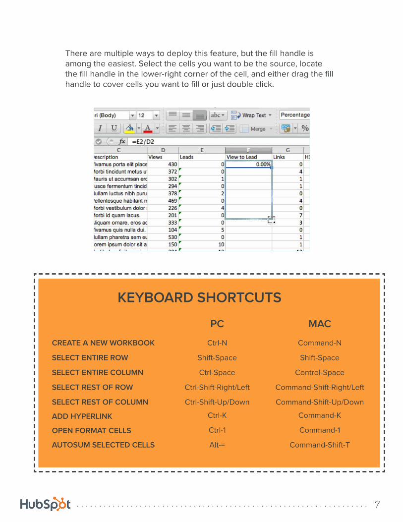
There are multiple ways to deploy this feature, but the fill handle is among the easiest. Select the cells you want to be the source, locate the fill handle in the lower-right corner of the cell, and either drag the fill handle to cover cells you want to fill or just double click.

KEYBOARD SHORTCUTS

CREATE A NEW WORKBOOK Ctrl-N

SELECT ENTIRE ROW Shift-Space

SELECT ENTIRE COLUMN Ctrl-Space

SELECT REST OF ROW Ctrl-Shift-Right/Left

SELECT REST OF COLUMN Ctrl-Shift-Up/Down

ADD HYPERLINK

OPEN FORMAT CELLS

AUTOSUM SELECTED CELLS

Ctrl-K

Ctrl-1

Alt-=

Command-N

Shift-Space

Control-Space

Command-Shift-Right/Left

Command-Shift-Up/Down

Command-K

Command-1

Command-Shift-T

PC MAC

. . . . . . . . . . . . . . . . . . . . . . . . . . . . . . . . . . . . . . . . . . . . . . . . . . . . . . . . . . . . . . . . . 8

Often, you’ll want to transform the items in a row of data into a column (or vice versa). It would take a lot of time to copy and paste each individual header. Not to mention, you may easily fall into one of the biggest, most unfortunate Excel traps: human error.

Instead, let Excel do the work for you. Go ahead and highlight the column or row you want to transpose. Right click and select “Copy.” Next, select the cells on your spreadsheet where you want your first row or column to begin. Right click on the cell, and then select “Paste Special.” When the module appears, choose the option to transpose.

Paste Special is one function I find myself coming back to time and time again. In the module, you can also choose between copying formulas, values, formats, or even column widths. This is especially helpful when it comes to copying the results of your pivot table (we’ll get there…) into a chart you can format and graph.

Paste Special

. . . . . . . . . . . . . . . . . . . . . . . . . . . . . . . . . . . . . . . . . . . . . . . . . . . . . . . . . . . . . . . . . 9

Have you ever seen a dollar sign in an Excel formula? It isn’t formatting numbers into currency. Instead, it makes sure that the exact column and row are kept consistent even if you copy the same formula in adjacent rows.

Excel is smart. When you refer to cell A5 from cell C5, for example, it defaults by notating its relative location. So in this case, you’re actually referring to a cell that’s two columns to the left (C minus A) and in the same row (5). When you copy this relative formula from one cell to another, it’ll adjust the values in the formula based on where it’s moved.

But what if you want that reference to stay the same, no matter where you copy the formula? Change the relative formula (=A5+C5) into an absolute formula by preceding the row and column values with dollar signs (=$A$5+$C$5).

Dollar Signs

If you haven’t already, download our Excel Practice Document to test your skills of the Basic Functions chapter. Insert a column after “Last Name.” Then combine the “First Name” and “Last Name” column using the concatenate function. Call your new column “Author” and delete “First Name” and “Last Name.”

TEST YOUR SKILLS:

. . . . . . . . . . . . . . . . . . . . . . . . . . . . . . . . . . . . . . . . . . . . . . . . . . . . . . . . . . . . . . . . . 10

VLOOKUPHave you ever had two sets of data on two different spreadsheets that you want to combine into a single spreadsheet? Yes, you could always open the two Excel documents and copy and paste cell by cell. But what happens when your spreadsheet contains hundreds of rows?

VLOOKUP is your answer. In short, this function uses a unique identifier -- like an email address or SKU number -- to match data from two different sources. For example, you might have some data from HubSpot and some from Salesforce that you want to combine together. Excel looks for a unique value in the leftmost column of a spreadsheet and fills a value in the same row from a column you specify in your other spreadsheet.

Before you use the formula, copy and paste your data so they are in two different sheets in the same Excel document. We’ll refer to Sheet 1 as the location where you want the final combined data to end up. Sheet 2 is the location of the data you want to transpose into Sheet 1.

Then, you’ll have to be absolutely sure that you have at least one column that appears identically in both Sheet 1 and Sheet 2. Sort your data (Data > Sort) in ascending order by this column and scour your data sets for discrepancies and extra spaces.

Here’s what the formula looks like:

=VLOOKUP(lookup value, table array, column number, [range lookup])

With values included, it becomes something like this:

=VLOOKUP(C2,Sheet2!A:B,2,FALSE)

If you think that looks like a mix of random numbers and letters, you’re not alone. Let’s break down each component.

• Lookup Value: This is the identical value you have in both spreadsheets. Choose the first value in Sheet 1 that you’re trying to find a match for.

. . . . . . . . . . . . . . . . . . . . . . . . . . . . . . . . . . . . . . . . . . . . . . . . . . . . . . . . . . . . . . . . . 11

• Table Array: This is the range of columns in Sheet 2 you want Excel to pull the data from. Be sure you’re highlighting both the column of data identical to your lookup value in Sheet 1 and the data that’s only available in Sheet 2 that you want to transpose. When you highlight this selection, Excel will enter a value like this into the formula: “Sheet2!A:B.”

• Column Index Number: This value tells Excel which column in Sheet 2 holds the new data you want to transpose into Sheet 1. Note, this is notated as a number, not by a letter. So the data in Column B would be referred to as “2” for the column number because it’s second from the left.

• Range Lookup: Enter FALSE to ensure you pull in only exact value matches.

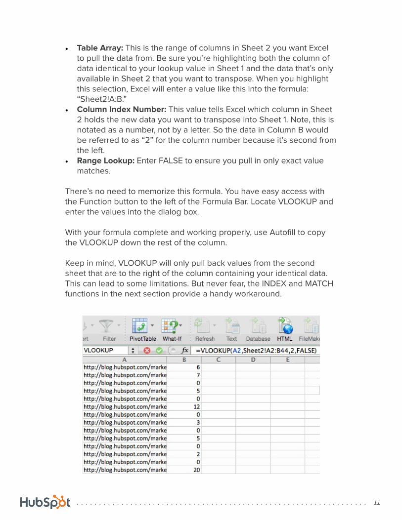
There’s no need to memorize this formula. You have easy access with the Function button to the left of the Formula Bar. Locate VLOOKUP and enter the values into the dialog box.

With your formula complete and working properly, use Autofill to copy the VLOOKUP down the rest of the column.

Keep in mind, VLOOKUP will only pull back values from the second sheet that are to the right of the column containing your identical data. This can lead to some limitations. But never fear, the INDEX and MATCH functions in the next section provide a handy workaround.

. . . . . . . . . . . . . . . . . . . . . . . . . . . . . . . . . . . . . . . . . . . . . . . . . . . . . . . . . . . . . . . . . 12

Like VLOOKUP, the INDEX and MATCH functions pull in data from another dataset into one central location. Here are the main differences:

• VLOOKUP is a much simpler formula. If you’re working with large data sets that would require thousands of lookups, then using the INDEX MATCH function will significantly decrease load time in Excel.

• INDEX MATCH formulas work right-to-left, whereas VLOOKUP formulas only work as a left-to-right lookup. In other words, if your lookup column is to the right of the results column, then you’d have to rearrange those columns in order to do a VLOOKUP. This can be tedious with large datasets and lead to errors.

Let’s take a look at the formula. You might notice the INDEX MATCH formula is actually the MATCH formula nested inside the INDEX formula.

=INDEX(table array, MATCH(lookup_value, lookup_array, match_type))

With actual values this becomes:

=INDEX(Sheet2!A:A, (MATCH(Sheet1!C:C,Sheet2!C:C,0)))

Let’s do another breakdown of these variables.

• Table Array: The range of columns on Sheet 2 containing the new data you want to bring over into Sheet 1. In the example above, this is just column A of Sheet 2.

• Lookup Value: This is the column in Sheet 1 that contains the identical values in both spreadsheets that you are trying to match. In the example, this is Column C of Sheet 1.

• Lookup Array: This is the column in Sheet 2 that contains identical values in both spreadsheets that Excel is searching. In the example, this is Column C of Sheet 2.

• Match Type: This tells Excel whether you want to return an exact match or the nearest match. To avoid unnecessary complexities, just remember to always use “0” here to get exact matches.

Enter this formula (or locate the INDEX and MATCH formulas with the Function button) into the first cell of the column where you want the combined information to live in Sheet 1. Autofill down.

INDEX MATCH

. . . . . . . . . . . . . . . . . . . . . . . . . . . . . . . . . . . . . . . . . . . . . . . . . . . . . . . . . . . . . . . . . 13

Let’s look back to our Excel Practice Document. In the first exercise, you were introduced to a spreadsheet of blog post data, including views and author. You’ll notice we’ve included a second sheet with lead counts for each blog post. Choose either the VLOOKUP function or INDEX MATCH to add lead numbers to each blog post. Insert this new “Lead” column to the right of “Views” in Sheet 1.

TEST YOUR SKILLS:

. . . . . . . . . . . . . . . . . . . . . . . . . . . . . . . . . . . . . . . . . . . . . . . . . . . . . . . . . . . . . . . . . 14

IF FUNCTIONSAt its most basic level, Excel’s IF function lets you see if a condition you set is true or false for a given value. If the condition is true, you get one result. If the condition is false, you get another result.

Before we dive in, let’s take a look at the this function’s syntax:

=IF(logical_test, value_if_true, [value_if_false])

With values, this could be:

=IF(A2>B2, “Over Budget”, “OK”)

In other words, if your spending (what’s in A2) is greater than your budget (what’s in B2), this IF function will make it easy to see. You can then filter the data and only see the line items where you’re going over budget.

The real power of the IF function, however, comes when you string multiple IF statements together, or “nest” them. This allows you to set multiple conditions, get more specific results, and ultimately organize your data into more manageable chunks.

Ranges are one way to segment your data for better analysis. For example, you can categorize data into values that are less than 10, 11 to 50, or 51 to 100.

=IF(B3<11,“10 or less”,IF(B3<51,“11 to 50”,IF(B3<100,“51 to 100”)))

. . . . . . . . . . . . . . . . . . . . . . . . . . . . . . . . . . . . . . . . . . . . . . . . . . . . . . . . . . . . . . . . . 15

The power of IF functions expands beyond simple true and false statements. Use the COUNTIF function to avoid manually counting how often a certain value or number appears. Here’s the formula:

=COUNTIF(range,criteria)

If you were looking for any occurrence of the subdirectory “marketing” in a URL in the D column, for instance, the formula would become:

=COUNTIF(D:D,”marketing”)

There are just two variables in this function:

• Range: This is the range that you want Excel to search for each instance of a specific value. If you are focusing on just one column, you could use “D:D” to indicate that both the first and last column are D. If you were looking at columns C and D, use “C:D”

• Criteria: This is whatever specific number or piece of text you want Excel to count for. Only use quotation marks if you want the result to be text instead of a number.

COUNTIF

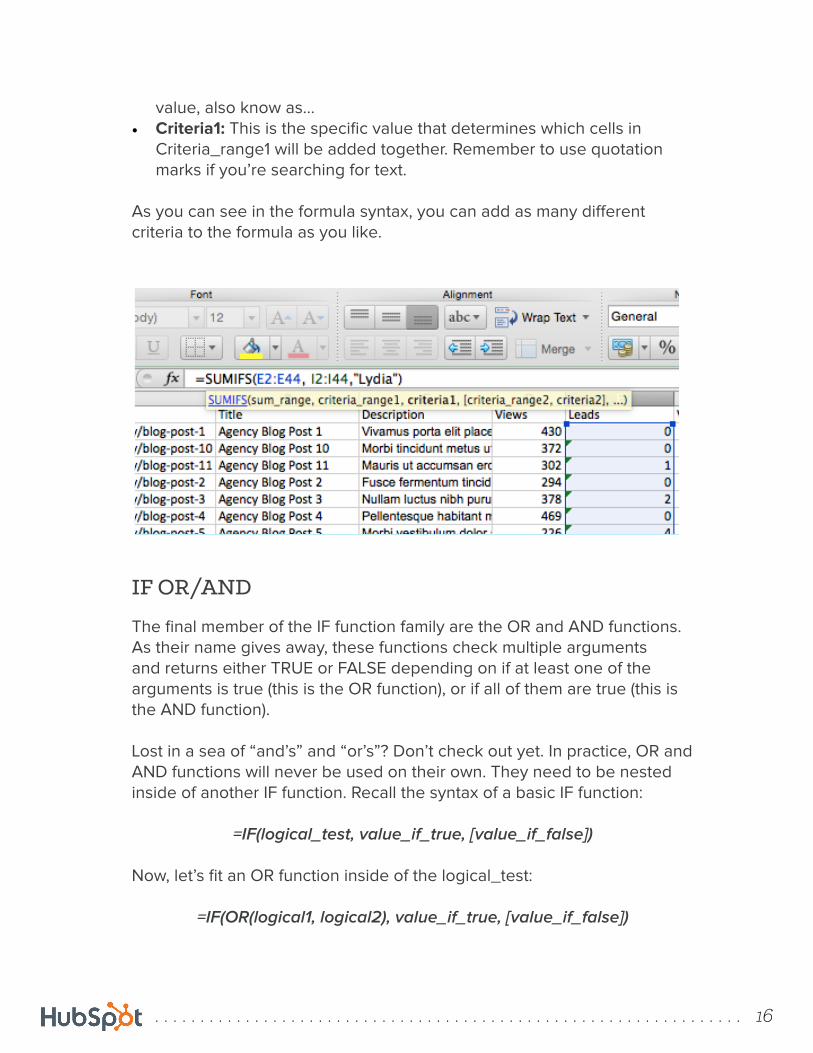
Ready to make IF function a bit more complex? Let’s say you want to analyze the number of leads your blog has generated -- but you only want to count leads from blog posts you wrote, not your entire team. With the SUMIFS function, you can add up cells that meet a certain criteria.

Here’s your formula:

=SUMIFS(sum_range, criteria_range1, criteria1, [criteria_range2, criteria 2],...)

That’s a lot of criteria. Let’s dive deeper into each part:

• Sum_range: This is the range of cells you’re going to add up• Criteria_range1: This is the range that is being searched for your first

SUMIFS

. . . . . . . . . . . . . . . . . . . . . . . . . . . . . . . . . . . . . . . . . . . . . . . . . . . . . . . . . . . . . . . . . 16

value, also know as...• Criteria1: This is the specific value that determines which cells in

Criteria_range1 will be added together. Remember to use quotation marks if you’re searching for text.

As you can see in the formula syntax, you can add as many different criteria to the formula as you like.

The final member of the IF function family are the OR and AND functions. As their name gives away, these functions check multiple arguments and returns either TRUE or FALSE depending on if at least one of the arguments is true (this is the OR function), or if all of them are true (this is the AND function).

Lost in a sea of “and’s” and “or’s”? Don’t check out yet. In practice, OR and AND functions will never be used on their own. They need to be nested inside of another IF function. Recall the syntax of a basic IF function:

=IF(logical_test, value_if_true, [value_if_false])

Now, let’s fit an OR function inside of the logical_test:

=IF(OR(logical1, logical2), value_if_true, [value_if_false])

IF OR/AND

. . . . . . . . . . . . . . . . . . . . . . . . . . . . . . . . . . . . . . . . . . . . . . . . . . . . . . . . . . . . . . . . . 17

In plain English, this combined formula allows you to return a value if one of two conditions are true, as opposed to just one. Ultimately with AND/OR functions, your formulas can be as simple or complex as you want them to be, as long as you understand the basics of the IF function.

Now that you’ve added the leads for each blog post in the previous application, let’s add up the total number of leads for a single author: Lydia Lee. Put that calculator away -- use the SUMIFS formula to find your total.

TEST YOUR SKILLS:

. . . . . . . . . . . . . . . . . . . . . . . . . . . . . . . . . . . . . . . . . . . . . . . . . . . . . . . . . . . . . . . . . 18

PIVOT TABLES

Let’s think back to back to the example of calculating leads from a list of blog posts. Like the previous scenario, you’re interested in calculating total leads generated by a single author. But instead of just wanting your own leads, now you want to compare the totals for each member of your team.

So, does this mean a bunch of SUMIFS formulas? Of course not. Once again, Excel gives us a much easier way. Allow me to introduce you to my absolute favorite tool of Excel: pivot tables.

With pivot tables, you can segment your data in a new sheet without altering the original organization. Pivot tables are flexible, allowing you to summarize large amounts of data (e.g. our spreadsheet of leads) and extract relevant information without using formulas.

To create the Pivot Table, go to Data > Pivot Table and a Wizard dialog box will appear for you to make a few choices. Excel will automatically populate your Pivot Table, but you can always change around the order of the data. Here, you have four options to choose from:

• Report Filter: This allows you to only look at certain rows in your dataset.

• Column Labels: This will be the headers in the new pivot table you’re creating. Feel free to add multiple labels to further analyze your data.

• Row Labels: These will be your rows in the new pivot table you’re creating. Important to note, both the Row and Column Labels of your Pivot Table can contain data from your original columns (e.g. Author can be dragged to either the Row or the Column label -- it just depends on how you want to see the data).

• Value: This section allows you to calculate the data specified by the Row Labels and Column Labels. You can sum, count, average, max, min, count numbers, or do a few other manipulations. In fact, by default, when you drag a field to Value it always does a count.

. . . . . . . . . . . . . . . . . . . . . . . . . . . . . . . . . . . . . . . . . . . . . . . . . . . . . . . . . . . . . . . . . 19

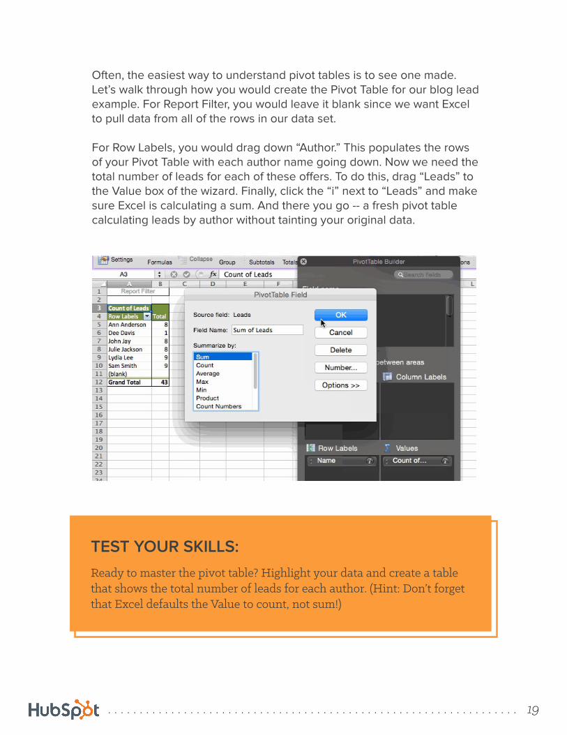
Often, the easiest way to understand pivot tables is to see one made. Let’s walk through how you would create the Pivot Table for our blog lead example. For Report Filter, you would leave it blank since we want Excel to pull data from all of the rows in our data set.

For Row Labels, you would drag down “Author.” This populates the rows of your Pivot Table with each author name going down. Now we need the total number of leads for each of these offers. To do this, drag “Leads” to the Value box of the wizard. Finally, click the “i” next to “Leads” and make sure Excel is calculating a sum. And there you go -- a fresh pivot table calculating leads by author without tainting your original data.

Ready to master the pivot table? Highlight your data and create a table that shows the total number of leads for each author. (Hint: Don’t forget that Excel defaults the Value to count, not sum!)

TEST YOUR SKILLS:

. . . . . . . . . . . . . . . . . . . . . . . . . . . . . . . . . . . . . . . . . . . . . . . . . . . . . . . . . . . . . . . . . 20

DATA VISUALIZATIONNow that you’ve mastered all of those formulas and functions, it’s time to put your analysis to good use. With the help of a beautiful graph, your audience (whether it’s a potential customer or your boss) will be able to synthesize and retain the content more effectively. Who knows? You might find just the edge to convince your boss to adopt inbound marketing or give you an extra sliver of budget.

Regardless of what you use the data for, you need it to be convincing. But if it’s not properly visualized, it can do more damage than good. In this section we’ll cover how to create a basic graph and a few common visualization errors every data-driven marketer should avoid.

One of the first decisions you’ll have to make is what type of graph to use. Bar charts and pie charts help you compare categories. Pie charts compare part of a whole and are often best when one of the categories is way larger than the others. Bar charts highlight incremental differences between categories. Finally, line charts are used to display trends over time.

To begin, highlight the data you want to morph into a chart, then choose “Charts” in the top navigation (or Insert > Chart if you have an older version of Excel). Then choose the graph most appropriate for your data.

Create a Basic Graph

Top Data Visualization Mistakes

Using non-solid lines in a line chart: Avoid distracting dashed and dotted lines. Instead, opt for solid lines and colors that are easy to distinguish from one another. Consider filling in the space below the line with a color to make it even more readable.

. . . . . . . . . . . . . . . . . . . . . . . . . . . . . . . . . . . . . . . . . . . . . . . . . . . . . . . . . . . . . . . . . 21

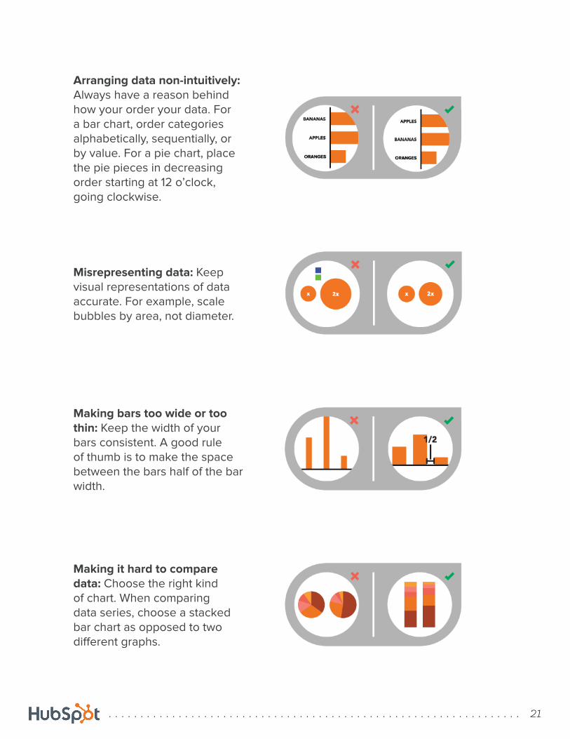
Arranging data non-intuitively: Always have a reason behind how your order your data. For a bar chart, order categories alphabetically, sequentially, or by value. For a pie chart, place the pie pieces in decreasing order starting at 12 o’clock, going clockwise.

Misrepresenting data: Keep visual representations of data accurate. For example, scale bubbles by area, not diameter.

Making bars too wide or too thin: Keep the width of your bars consistent. A good rule of thumb is to make the space between the bars half of the bar width.

Making it hard to compare data: Choose the right kind of chart. When comparing data series, choose a stacked bar chart as opposed to two different graphs.

. . . . . . . . . . . . . . . . . . . . . . . . . . . . . . . . . . . . . . . . . . . . . . . . . . . . . . . . . . . . . . . . . 22

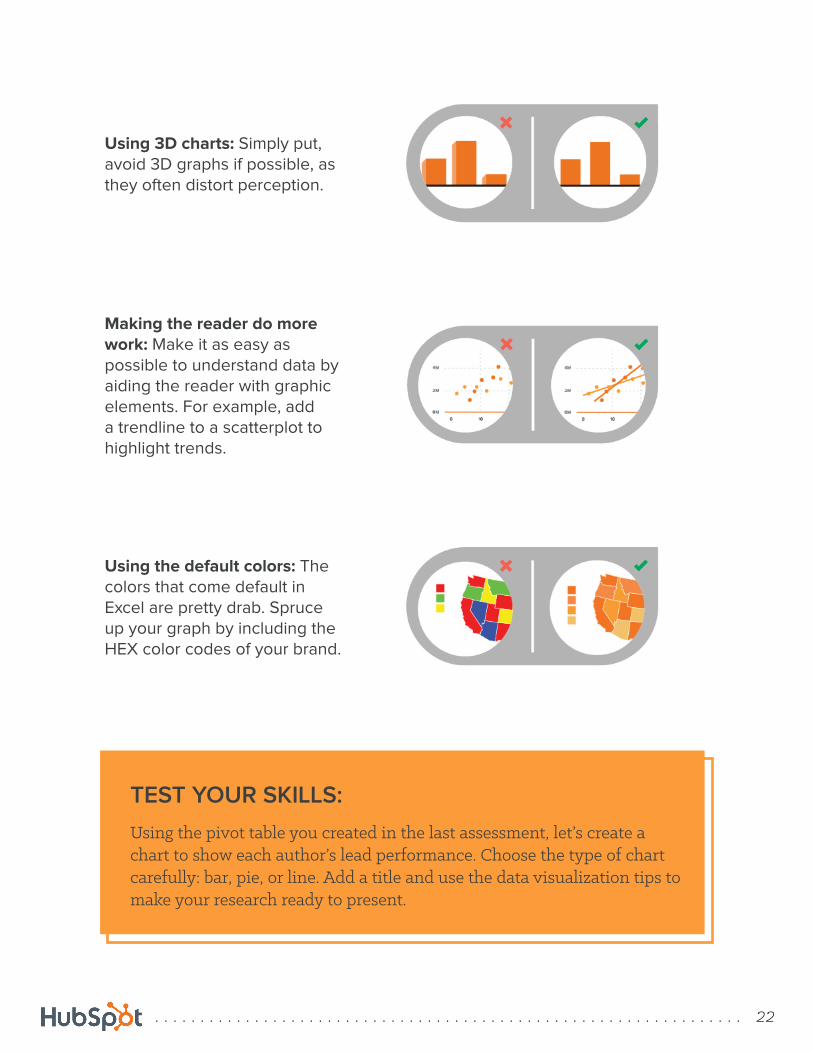
Using 3D charts: Simply put, avoid 3D graphs if possible, as they often distort perception.

Making the reader do more work: Make it as easy as possible to understand data by aiding the reader with graphic elements. For example, add a trendline to a scatterplot to highlight trends.

Using the default colors: The colors that come default in Excel are pretty drab. Spruce up your graph by including the HEX color codes of your brand.

Using the pivot table you created in the last assessment, let’s create a chart to show each author’s lead performance. Choose the type of chart carefully: bar, pie, or line. Add a title and use the data visualization tips to make your research ready to present.

TEST YOUR SKILLS:

. . . . . . . . . . . . . . . . . . . . . . . . . . . . . . . . . . . . . . . . . . . . . . . . . . . . . . . . . . . . . . . . . 23

FINAL TOUCHESWith your charts made and trends identified, are you ready to present all of your hard work? Likely, there are a few final touches to ensure your data is organized and intuitive for whoever gets ahold of your spreadsheet. Below are just a few tricks to make your data look worthy of the design-savvy marketer you are.

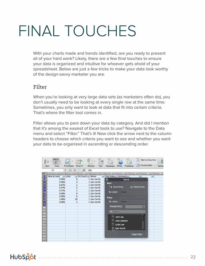
When you’re looking at very large data sets (as marketers often do), you don’t usually need to be looking at every single row at the same time. Sometimes, you only want to look at data that fit into certain criteria. That’s where the filter tool comes in.

Filter allows you to pare down your data by category. And did I mention that it’s among the easiest of Excel tools to use? Navigate to the Data menu and select “Filter.” That’s it! Now click the arrow next to the column headers to choose which criteria you want to see and whether you want your data to be organized in ascending or descending order.

Filter

. . . . . . . . . . . . . . . . . . . . . . . . . . . . . . . . . . . . . . . . . . . . . . . . . . . . . . . . . . . . . . . . . 24

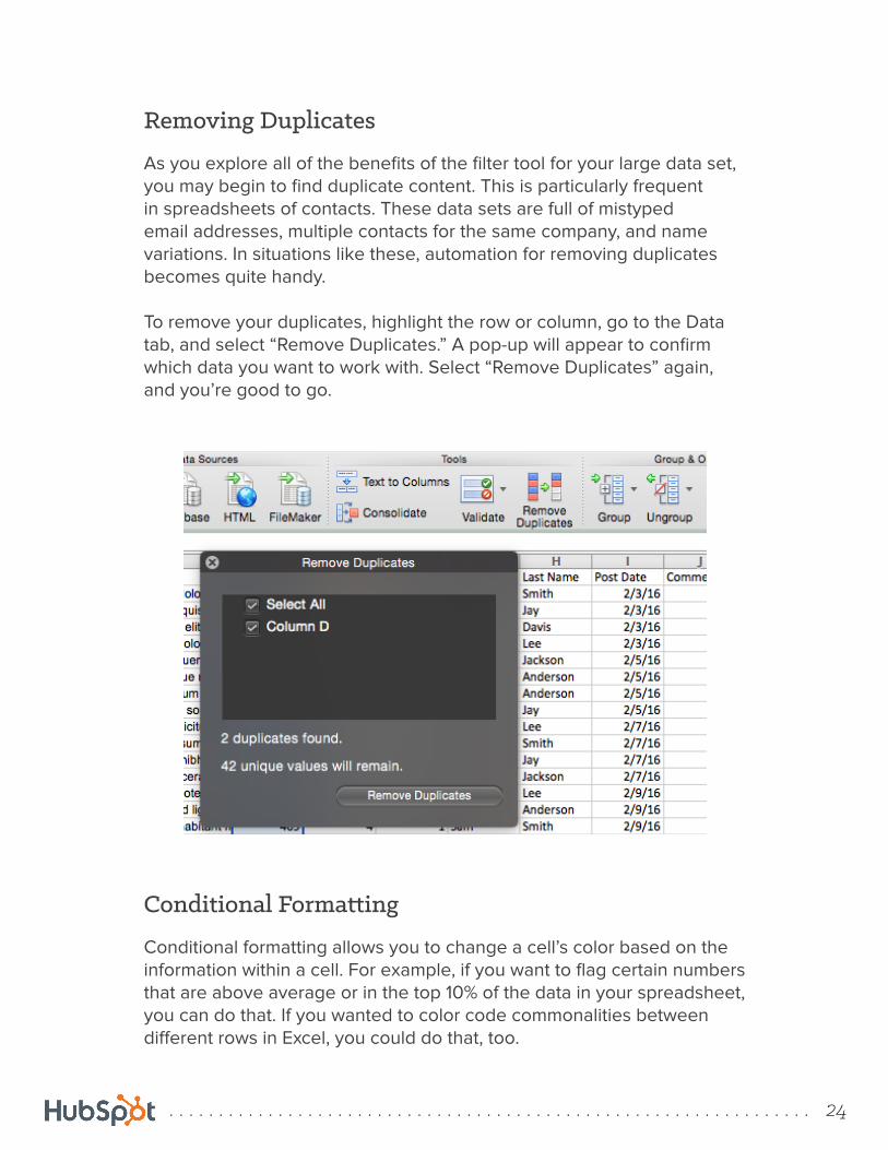
As you explore all of the benefits of the filter tool for your large data set, you may begin to find duplicate content. This is particularly frequent in spreadsheets of contacts. These data sets are full of mistyped email addresses, multiple contacts for the same company, and name variations. In situations like these, automation for removing duplicates becomes quite handy.

To remove your duplicates, highlight the row or column, go to the Data tab, and select “Remove Duplicates.” A pop-up will appear to confirm which data you want to work with. Select “Remove Duplicates” again, and you’re good to go.

Removing Duplicates

Conditional formatting allows you to change a cell’s color based on the information within a cell. For example, if you want to flag certain numbers that are above average or in the top 10% of the data in your spreadsheet, you can do that. If you wanted to color code commonalities between different rows in Excel, you could do that, too.

Conditional Formatting

. . . . . . . . . . . . . . . . . . . . . . . . . . . . . . . . . . . . . . . . . . . . . . . . . . . . . . . . . . . . . . . . . 25

To get started, highlight the group of cells you want to use conditional formatting on. Then choose “Conditional Formatting” from the Home menu and select your logic from the dropdown. If you don’t see the rule you need, you can customize it. Then choose the color that will correspond with your rule.

As you’ve probably noticed, Excel has a lot of features to make crunching numbers and analyzing your data quick and easy. But if you ever spent some time formatting a sheet to your liking, you know it can get a bit tedious.

Don’t waste time repeating the same formatting commands over and over again. Use the format painter to easily copy the formatting from one area of the worksheet to another. To do so, choose the cell you’d like to replicate, then select the format painter option (paintbrush icon) from the top toolbar.

Format Painter

. . . . . . . . . . . . . . . . . . . . . . . . . . . . . . . . . . . . . . . . . . . . . . . . . . . . . . . . . . . . . . . . . 26

For our final knowledge check, let’s switch back to Sheet 1 of your practice document and analyze our view-to-lead conversion rates. Insert a “View-to-Lead” column after “Leads.” Calculate your conversion rate for each blog post and format the column as percentages. Then, use conditional formatting to highlight any rate that is above 2% in green.

TEST YOUR SKILLS:

You’ve done your part and learned everything you need to be an Excel master. Now let us take off some of the

load. Take your pick from our library of Excel templates to simplify your most crucial marketing tasks.

Take control of your multifacet-ed budget with these templates

in Excel and Google Sheets.

8 Marketing Budget Templates

Plan and optimize your blogging with these templates.

Blog Editorial Calendar Templates

Easily plan your content and manage your social media net-

works.

Social Media Content Calendar Template

Prepare for SMART Marketing with this Goal-Setting Excel

Template.

Determine Your SMART Goals

Plan your SEO in advance for a more scalable solution.

On-Page SEO Template

Determine the dollar value of your leads to build a service

level agreement.

Leads Goal Template