How to model quantum plasmas - master-mcn

Fields Institute CommunicationsVolume 00, 0000

How to model quantum plasmas

Giovanni ManfrediLaboratoire de Physique des Milieux Ionises et Applications

CNRS and Universite Henri Poincare, BP 239F-54506 Vandoeuvre-les-Nancy

France

Abstract. Traditional plasma physics has mainly focused on regimescharacterized by high temperatures and low densities, for which quantum-mechanical effects have virtually no impact. However, recent technolog-ical advances (particularly on miniaturized semiconductor devices andnanoscale objects) have made it possible to envisage practical applica-tions of plasma physics where the quantum nature of the particles playsa crucial role. Here, I shall review different approaches to the modelingof quantum effects in electrostatic collisionless plasmas. The full kineticmodel is provided by the Wigner equation, which is the quantum analogof the Vlasov equation. The Wigner formalism is particularly attractive,as it recasts quantum mechanics in the familiar classical phase space,although this comes at the cost of dealing with negative distributionfunctions. Equivalently, the Wigner model can be expressed in termsof N one-particle Schrodinger equations, coupled by Poisson’s equation:this is the Hartree formalism, which is related to the ‘multi-stream’ ap-proach of classical plasma physics. In order to reduce the complexity ofthe above approaches, it is possible to develop a quantum fluid model bytaking velocity-space moments of the Wigner equation. Finally, certainregimes at large excitation energies can be described by semiclassicalkinetic models (Vlasov-Poisson), provided that the initial ground-stateequilibrium is treated quantum-mechanically. The above models arevalidated and compared both in the linear and nonlinear regimes.

1 Introduction

Plasma physics deals with the N -body dynamics of a system of charged par-ticles interacting via electromagnetic forces. The study of plasmas arose in theearly twentieth century when scientists got interested in the physics of gas dis-charges. After World War II, plasmas became the object of intensive experimentaland theoretical research, mainly because of the potential applications of nuclearfusion, both military (hydrogen bomb) and peaceful (energy production throughcontrolled thermonuclear fusion). In parallel, plasma physics was also developed

c©0000 American Mathematical Society

1

2 Giovanni Manfredi

by astrophysicists and geophysicists, which is not surprising, as it is thought thatabout 90% of all matter in the visible universe exists in the form of a plasma. Moreprecisely, plasmas are observed in the Sun surface, the earth’s magnetosphere, andthe interplanetary and interstellar media.

Both fusion and space plasmas are characterized by regimes of high tempera-ture and low density, for which quantum effects are totally negligible 1. However,physical systems where both plasma and quantum effects coexist do occur in nature,the most obvious example being the electron gas in an ordinary metal. In metals,valence electrons are not attached to a particular nucleus, but rather behave as freeparticles, which is why metals make good electric conductors. Although some levelof understanding of metallic properties is achieved by considering noninteractingelectrons, a more accurate description can be obtained by treating the electron pop-ulation as a plasma, globally neutralized by the lattice ions. At room temperatureand standard metallic densities, quantum effects can no longer be ignored, so thatthe electron gas constitutes a true quantum plasma.

For ordinary metals, however, the properties of the electron population (bandstructure, thermodynamic properties) are mainly determined by the presence of aregular ion lattice, typical plasma effects being only a higher order correction. Inrecent years, though, there has been tremendous progress in the manipulation ofmetallic nanostructures (metal clusters, nanoparticles, thin metal films) constitutedof a small number of atoms (typically 10− 105) [1, 2, 3, 4, 5]. For such objects, nounderlying ionic lattice exists, so that the dynamics of the electron population isprincipally governed by plasma effects, at least for large enough systems. Further,the development of ultrafast (femtosecond and, more recently, attosecond) lasersources makes it possible to probe the electron dynamics in metallic nanostructureson the typical time scale of plasma phenomena, which is indeed of the order of thefemtosecond. Metallic nanostructures thus constitute an ideal arena to study thedynamical properties of quantum plasmas.

Another possible application of quantum plasmas arises from semiconductorphysics [6, 7, 8, 9, 10]. Even though the electron density in semiconductors ismuch lower than in metals, the great degree of miniaturization of today’s electroniccomponents is such that the de Broglie wavelength of the charge carriers can becomparable to the spatial variation of the doping profiles. Hence, typical quantummechanical effects, such as tunneling, are expected to play a central role in thebehavior of electronic components to be constructed in the next years.

Finally, quantum plasmas also occur in some astrophysical objects under ex-treme conditions of temperature and density, such as white dwarf stars, where thedensity is some ten order of magnitudes larger than that of ordinary solids [11].Because of such large densities, a white dwarf can be as hot as a fusion plasma (108

K), but still behave quantum-mechanically.A classical system of charged particles qualifies as a plasma if it is quasineutral

and if collective effects play a significant role in the dynamics [12]. ‘Quasineutral-ity’ means that charge separation can only exist on a short distance, which, forclassical plasmas, is given by the Debye length. On distances larger than the Debyelength, the plasma is basically neutral, except for small fluctuations. By ‘collective

1Quantum effects do play an important role, for example, in determining the fusion crosssections. But this is a nuclear physics rather than a plasma physics issue. What we mean isthat the dynamics and thermodynamics of fusion and space plasmas are completely unaffected byquantum corrections.

How to model quantum plasmas 3

effects’ we mean particle motions that depend not only on local conditions, butalso – indeed principally – on the positions and velocities of all other particles inthe plasma. (In solid state and nuclear physics, collective effects are usually called‘mean-field’ effects, because they arise from the average field created by all theparticles). Such collective behavior is possible because of the long-range natureof electromagnetic forces. In contrast, for neutral gases, the dominant interactionmechanism is provided by short-range molecular forces of the Lennard-Jones type:individual molecules thus move undisturbed in the gas until they make a collisionwith another molecule (which occurs when the interaction potentials overlap). Itshould be added that real plasmas are often only partially ionized, so that a frac-tion of neutral molecules is also present. In order to have true plasma behavior,we must therefore require that the collision rates of electrons and ions with theneutral molecules be relatively low compared to typical collective phenomena. Inthe present work, we shall avoid this issue altogether by restricting our analysis tothe simpler case of fully ionized gases.

When quantum effects start playing a role, the above picture gets more compli-cated, as an additional length scale is introduced, namely the de Broglie wavelengthof the charged particles, λB = ~/mv. The de Broglie wavelength roughly repre-sents the spatial extension of the particle wave function – the larger it is, the moreimportant quantum effects are. From the definition of λB , it is clear that quan-tum behavior will be reached much more easily for the electrons than for the ions,due to the large mass difference. Indeed, in all practical situations, even the mostextreme, the ion dynamics is always classical, and only the electrons need to betreated quantum-mechanically. In the present paper, we shall always refer implic-itly to electrons when discussing quantum effects. In addition, only electrostatic(Coulomb) interactions will be considered. Magnetic fields do introduce novel andinteresting effects, but the fundamental properties of quantum plasmas are alreadypresent in the purely electrostatic scenario.

In the rest of this paper, we shall first obtain a number of qualitative results byusing simple arguments from dimensional analysis. This will be useful to extractthe relevant dimensionless parameters that determine the various physical regimes(classical/quantum, collisionless/collisional). Subsequently, we shall derive and il-lustrate several mathematical models that are appropriate to describe the dynamicsof a quantum plasma in the collisionless regime.

2 Physical regimes for classical and quantum plasmas

In this section, we shall derive a number of parameters that represent the typi-cal length, time, and velocity scales in a classical or quantum plasma. These can beobtained using elementary considerations based on dimensional analysis. Of course,more detailed studies would be necessary to understand how such parameters ac-tually intervene in real physical phenomena (for instance, whether a certain timescale represents a typical oscillation frequency, or rather a damping rate). Here, weshall derive the algebraic expression for these quantities and simply state, withoutproof, what they represent physically.

In addition, it will also be important to establish certain dimensionless parame-ters. Dimensionless parameters allow us to discriminate between different physicalregimes, characterized by situations where one effect dominates over another. Inparticular, we shall look for parameters that define whether a plasma is classical or

4 Giovanni Manfredi

quantum, and whether it is dominated by individual effects (collisional) or collectiveeffects (collisionless).

2.1 Classical plasmas. We consider a plasma of number density n, composedof particles (typically, electrons) with mass m and electric charge e, interacting viaCoulomb forces (hence the electric permittivity ε0). With these four parameters,we are able to construct a quantity that has the dimensions of an inverse time, i.e.a frequency:

ωp =(

e2n

mε0

)1/2

. (2.1)

The latter quantity is known as the plasma frequency and it represents thetypical oscillation frequency for electrons immersed in a neutralizing backgroundof positive ions, which is supposed to be motionless because of the large ion mass.The oscillations arise from the fact that, when a portion of the plasma is depletedof some electrons (thus creating a net positive charge), the resulting Coulomb forcetends to pull back the electrons towards the excess positive charge. Due to theirinertia, the electrons will not simply replenish the positive region, but travel furtheraway thus re-creating an excess positive charge. In the absence of collisions, thiseffect gives rise to undamped electron oscillations at the plasma frequency.

Note that the plasma frequency is independent on the temperature. If we dointroduce a finite temperature T , then we can construct a typical velocity:

vT =(

kBT

m

)1/2

, (2.2)

where kB is Boltzmann’s constant. This is the thermal velocity, which represents,just like in ordinary gases, the typical speed due to random thermal motion.

By combining the above two quantities, one can define a typical length scale,the Debye length:

λD =vT

ωp=

(ε0kBT

ne2

)1/2

. (2.3)

The Debye length describes the important phenomenon of electrostatic screening: ifan excess positive charge is introduced in the plasma, it will be rapidly surroundedby a cloud of electrons (which are more mobile and thus react quickly). As a result,the positive charge will be partially screened and will be virtually ‘invisible’ toother particles situated at a large enough distance. Quantitatively, this amounts tosaying that the electrostatic potential generated by an excess charge does not fall,like in vacuum, as 1/r, but rather obeys a Yukawa-like potential exp(−r/λD)/r,which of course decays much more quickly and on a distance of the order of theDebye length. The Debye screening is at the origin of one of the most crucial of allplasma properties, namely quasineutrality: charge separation in a plasma can existonly on scales smaller than λD, but it is screened out at larger sales.

Let us now try to construct a dimensionless parameter using the above quanti-ties: m, e, ε0, n, and T . It is easily seen that only one such parameter exists, andit reads as

gC =e2n1/3

ε0kBT. (2.4)

This is known as the (classical) graininess parameter or coupling parameter.It is illuminating to show that gC can be written as the ratio of the interaction(electric) energy Eint to the average kinetic energy Ekin. Indeed, for particles


situated at typical interparticle distance d = n−1/3, one has Eint = e2/(ε0d) andEkin = kBT , which immediately yields the expression (2.4).

The expression gC = Eint/Ekin allows us to guess the physical relevance of thecoupling parameter. When gC is small, the plasma is dominated by thermal ef-fects, whereas two-body Coulomb interactions (i.e. binary collisions) remain weak.In this regime, the main field acting on the charged particles is the nonlocal meanfield, which is responsible for typical collective effects. This is known as the colli-sionless regime. On the contrary, when gC ' 1 or larger, binary collisions cannotbe neglected and the plasma is said to be collisional or strongly coupled. We alsonote that, following (2.4), classical plasmas are collisionless at high temperaturesand low densities.

Alternatively, gC can be written as the inverse of the number of particles con-tained in a volume of linear dimension λD, raised to a certain power:

gC =(

1nλ3

D

)2/3

. (2.5)

This shows that a plasma is collisionless when the Debye screening is effective, i.e.when a large number of electrons are available in a Debye volume.

2.2 Quantum plasmas. Quantum effects can be measured by the thermalde Broglie wavelength of the particles composing the plasma

λB =~

mvT, (2.6)

which roughly represents the spatial extension of a particle’s wave function due toquantum uncertainty. For classical regimes, the de Broglie wavelength is so smallthat particles can be considered as pointlike (except, as mentioned in the Introduc-tion, when computing collision cross-sections), therefore there is no overlapping ofthe wave functions and no quantum interference. On this basis, it is reasonable topostulate that quantum effects start playing a significant role when the de Brogliewavelength is similar to or larger than the average interparticle distance n−1/3, i.e.when

nλ3B ≥ 1 . (2.7)

On the other hand, it is well known from the statistical mechanics of ordinarygases [13] that quantum effects become important when the temperature is lowerthan the so-called Fermi temperature TF , defined as

kBTF ≡ EF =~2

2m(3π2)2/3 n2/3 , (2.8)

where we have also defined the Fermi energy EF . When T approaches TF , therelevant statistical distribution changes from Maxwell-Boltzmann to Fermi-Dirac.Now, it is easy to see that the ratio χ ≡ T/TF is simply related to the dimensionlessparameter nλ3

B discussed above:

χ ≡ TF

T=

12

(3π2)2/3 (nλ3B)2/3. (2.9)

Thus, quantum effects become important when χ ≥ 1.We now want to establish the typical space, time, and velocity scales for a

quantum plasma, as well as the relevant dimensionless parameters. First of all,we stress that simple expressions can be found only in the limiting cases T À TF

(corresponding to the classical case treated previously) and T ¿ TF , which is

6 Giovanni Manfredi

the ‘deeply quantum’ (fully degenerate) regime that we are going to analyze. Ofcourse, there will be a smooth transition between the two regimes, but this cannotbe treated using straightforward dimensional arguments.

Concerning the typical time scale for collective phenomena, this is still given bythe inverse of the plasma frequency (2.1), even in the quantum regime. However, thethermal speed becomes meaningless in the very low temperature limit, and shouldbe replaced by the typical velocity characterizing a Fermi-Dirac distribution. Thisis the Fermi velocity:

vF =(

2EF

m

)1/2

=~m

(3π2 n)1/3 . (2.10)

With the plasma frequency and the Fermi velocity, we can define a typicallength scale

λF =vF

ωp, (2.11)

which is the quantum analog of the Debye length. Just like the Debye length, λF

describes the scale length of electrostatic screening in a quantum plasma.The quantum coupling parameter can be defined as the ratio of the interaction

energy Eint to the average kinetic energy Ekin. The interaction energy is the sameas in the classical case, whereas the kinetic energy is now given by the Fermienergy Ekin = EF . With these assumptions, one can write the quantum couplingparameter as

gQ ≡ Eint

EF=

2(3π2)2/3

e2m

~2ε0 n1/3∼

(1

nλ3F

)2/3

∼(~ωp

EF

)2

, (2.12)

where we have left out proportionality constants for sake of clarity. The thirdexpression of gQ in (2.12) is completely analogous to the classical one when onesubstitutes λF → λD. The last expression is more interesting, as it has no classicalcounterpart: it describes the coupling parameter as the ratio of the ‘plasmon energy’~ωp (energy of an elementary excitation associated to an electron plasma wave) tothe Fermi energy 2.

The quantum collisionless regime (where collective, mean-field effects dominate)is again defined as the regime where the quantum coupling parameter is small. From(2.12), it appears that a quantum plasma is ‘more collective’ at larger densities, incontrast to a classical plasma [see (2.4)]. This may seem surprising, but can beeasily understood by invoking Pauli’s exclusion principle, according to which twofermions cannot occupy the same quantum state. In a fully degenerate fermion gas,all low-energy states are occupied: if we add one more particle to the gas, it willnecessarily be in a high-energy state. Therefore, by increasing the gas density, weautomatically increase its average kinetic energy, which, in virtue of (2.12), reducesthe value of gQ.

2.3 Plasma regimes. We have so far defined three dimensionless parametersthat determine whether the plasma is classical or quantum, and, in either case,whether it is collisional or collisionless:

1. χ = TF /T : classical/quantum2. gC : collisional/collisionless (classical regime)

2gQ is directly proportional to the parameter rs/a0 (where a0 is Bohr’s radius), commonly

used in solid state physics [14].


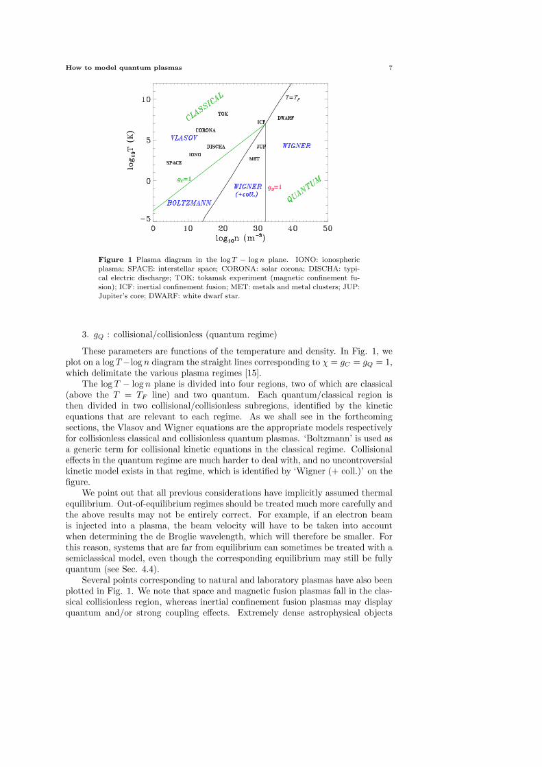
Figure 1 Plasma diagram in the log T − log n plane. IONO: ionosphericplasma; SPACE: interstellar space; CORONA: solar corona; DISCHA: typi-cal electric discharge; TOK: tokamak experiment (magnetic confinement fu-sion); ICF: inertial confinement fusion; MET: metals and metal clusters; JUP:Jupiter’s core; DWARF: white dwarf star.

3. gQ : collisional/collisionless (quantum regime)

These parameters are functions of the temperature and density. In Fig. 1, weplot on a log T−log n diagram the straight lines corresponding to χ = gC = gQ = 1,which delimitate the various plasma regimes [15].

The log T − log n plane is divided into four regions, two of which are classical(above the T = TF line) and two quantum. Each quantum/classical region isthen divided in two collisional/collisionless subregions, identified by the kineticequations that are relevant to each regime. As we shall see in the forthcomingsections, the Vlasov and Wigner equations are the appropriate models respectivelyfor collisionless classical and collisionless quantum plasmas. ‘Boltzmann’ is used asa generic term for collisional kinetic equations in the classical regime. Collisionaleffects in the quantum regime are much harder to deal with, and no uncontroversialkinetic model exists in that regime, which is identified by ‘Wigner (+ coll.)’ on thefigure.

We point out that all previous considerations have implicitly assumed thermalequilibrium. Out-of-equilibrium regimes should be treated much more carefully andthe above results may not be entirely correct. For example, if an electron beamis injected into a plasma, the beam velocity will have to be taken into accountwhen determining the de Broglie wavelength, which will therefore be smaller. Forthis reason, systems that are far from equilibrium can sometimes be treated with asemiclassical model, even though the corresponding equilibrium may still be fullyquantum (see Sec. 4.4).

Several points corresponding to natural and laboratory plasmas have also beenplotted in Fig. 1. We note that space and magnetic fusion plasmas fall in the clas-sical collisionless region, whereas inertial confinement fusion plasmas may displayquantum and/or strong coupling effects. Extremely dense astrophysical objects

8 Giovanni Manfredi

such as white dwarf stars are definitely quantum and collisionless, even thoughthey are as hot as fusion or solar plasmas.

3 Electrons in metals and metallic nanostructures: Pauli blocking

The typical quantum coupling parameter for ordinary metals is larger thanunity, so that, in principle, electron-electron collisions are as important as collec-tive effects. If that were really the case, one should abandon collisionless modelsaltogether and resort to the full N -body problem. This is hardly a feasible task.Fortunately, however, the effect known as Pauli blocking reduces the collision ratequite dramatically in most cases of interest. This occurs when the electron distri-bution is close to the Fermi-Dirac equilibrium at relatively low temperatures. Thefundamental point is that, when all lower levels are occupied, the exclusion principleforbids a vast number of transitions that would otherwise be possible [14]. In par-ticular, at strictly zero temperature, all electrons have energies below EF , and notransition is possible, simply because there are no available states for the electronsto occupy. At moderate temperatures, only electrons within a shell of thicknesskBT about the Fermi surface (i.e. the region where E = EF ) can undergo collisions(this shell is delimited by the two vertical lines in Fig. 2). For such electrons, thee-e collision rate (inverse of the lifetime τee) is proportional to kBT/~ (this is aform of the uncertainty principle, energy × time = const.). The average collisionrate is obtained by multiplying the previous expression by the fraction of electronspresent in the shell of thickness T about the Fermi surface, which is ∼ T/TF . Oneobtains

νee ∼ kBT 2

~ TF. (3.1)

In normalized units, this expression reads as

νee

ωp=

EF

~ωp

(T

TF

)2

=1

g1/2Q

(T

TF

)2

(3.2)

Thus, νee < ωp in the region where T < TF and gQ > 1, which is the relevantone for metallic electrons (Fig. 1). Restoring dimensional units, we find that, atroom temperature, τee ' 10−10 s, which is much larger than the typical collisionlesstime scale τp = 2πω−1

p ' 10−15 s = 1 fs. In addition, the typical time scale forelectron-lattice collisions τei ' 10−14 s = 10 fs is also larger than τp. Therefore, itappears that a collisionless regime is indeed relevant on a time scale of the order ofthe femtosecond.

A word of caution is in order, however, not to overestimate the effect ofPauli blocking. The above considerations are valid at thermodynamic equilibrium,whereas many more transitions are allowed for out-of-equilibrium electrons. There-fore, for strongly excited systems where many nonequilibrium electrons are present,the collision frequency may be larger than the simple estimate given in (3.2).

Some typical parameters for metallic electrons (gold) at room temperature aresummarized in Table 1. We note that τp, the typical collisionless time scale, is of theorder of the femtosecond. With the recent development of ultrafast laser sourceswith femtosecond period, it is therefore possible to probe the mean-field propertiesof metallic nanostructures. For example, the electron dynamics in thin gold filmsexcited with femtosecond lasers was studied experimentally in several works [2, 3].


Figure 2 Fermi-Dirac energy distribution for a case with T/TF = 0.1. Thevertical lines define a shell of thickness kBT around the Fermi surface.

We also point out that λF , the typical collisionless length scale, is of the order ofthe Angstrom, which is comparable to the typical atomic size.

Table 1 Typical parameters for electrons in gold at room temperature

n 5.9× 1028 m−3

T 300 Kωp 1.37× 1016 s−1

τp 0.46 fsτie 30 fsTF 6.4× 104 KEF 5.53 eVvF 1.4× 106 ms−1

λF 1× 10−10 mgQ 12.7

rs/a0 3

4 Models

The most fundamental model for the quantum N -body problem is the Schrodin-ger equation for the N -particle wave function ψ(x1, x2, . . . , xN , t). Obviously, thisis an unrealistic task, both for analytical calculations and numerical simulations.A drastic, but useful and to some extent plausible, simplification can be achievedby neglecting two-body (and higher order) correlations. This amounts to assumethat the N -body wave function can be factored into the product of N one-bodyfunctions:

ψ(x1, x2, . . . , xN , t) = ψ1(x1, t) ψ2(x2, t) . . . ψN (xN , t). (4.1)For fermions, a weak form of the exclusion principle is satisfied if none of the wavefunctions on the right-hand side of (4.1) are identical 3.

3A stronger version of the exclusion principle requires that ψ(x1, x2, . . . , xN , t) is antisym-metric, i.e. that it changes sign when two of its arguments are interchanged. This can be achievedby taking, instead of the single product of N wave functions as in (4.1), a linear combinations of

10 Giovanni Manfredi

The assumption of weak correlation between the particles is satisfied, as wehave seen, when the quantum coupling parameter gQ is small. The set of N one-body wave functions is known as a quantum mixture (or quantum mixed state) andis usually represented by a density matrix

ρ(x, y, t) =N∑

α=1

pαψα(x, t) ψ∗α(y, t), (4.2)

where, for clarity, we have assumed the same normalization∫

ψα2dx = 1 for all

wave functions and then introduced the occupation probabilities pα.Both the Wigner and Hartree models described below are completely equivalent

to models based on the density matrix formalism (Von Neumann equation).

4.1 Wigner-Poisson. The Wigner representation [16] is a useful tool to ex-press quantum mechanics in a phase space formalism (for reviews see [17, 18, 19]).As detailed above, a generic quantum mixed state can be described by N single-particle wave functions ψα(x, t) each characterized by a probability pα satisfying∑N

α=1 pα = 1. The Wigner function is a function of the phase space variables (x, v)and time, which, in terms of the single-particle wave functions, reads as

f(x, v, t) =N∑

α=1

m

2π~pα

∫ +∞

−∞ψ∗α

(x +

λ

2, t

)ψα

(x− λ

2, t

)eimvλ/~ dλ (4.3)

(we restrict our discussion to one-dimensional cases, but all results can easily begeneralized to three dimensions). It must be stressed that the Wigner function,although it possesses many useful properties, is not a true probability density, asit can take negative values. However, it can be used to compute averages just likein classical statistical mechanics. For example, the expectation value of a genericquantity A(x, v) is defined as:

〈A〉 =∫ ∫

f(x, v)A(x, v)dxdv∫ ∫f(x, v)dxdv

, (4.4)

and yields the correct quantum-mechanical value 4. In addition, the Wigner func-tion reproduces the correct quantum-mechanical marginal distributions, such as thespatial density:

n(x, t) =∫ +∞

−∞f(x, v, t) dv =

N∑α=1

pα | ψα |2 . (4.5)

We also point out that, of course, not all functions of the phase space variablesare genuine Wigner functions, as they cannot necessarily be written in the form(4.3). In general, although it is trivial to find the Wigner function given the N wavefunctions that define the quantum mixture, the inverse operation is not generallyfeasible. Indeed, there are no simple rules to establish whether a given function ofx and v is a genuine Wigner function. For a more detailed discussion on this issue,and some practical recipes to construct genuine Wigner functions, see [20].

all products obtained by permutations of the arguments, with weights ±1 (Slater determinant)[14]. This is at the basis of Fock’s generalization of the Hartree model, as pointed out in Sec. 4.2.

4For variables whose corresponding quantum operators do not commute (such as xv), (4.4)must be supplemented by an ordering rule, known as Weyl’s rule [19].


The Wigner function obeys the following evolution equation:

∂f

∂t+ v

∂f

∂x+

em

2iπ~2

∫ ∫dλ dv′eim(v−v′)λ/~

[φ

(x +

λ

2

)− φ

(x− λ

2

)]f(x, v′, t) = 0 , (4.6)

where φ(x, t) is the self-consistent electrostatic potential. Developing the integralterm in (4.6) up to order O(~2) we obtain

∂f

∂t+ v

∂f

∂x− e

m

∂φ

∂x

∂f

∂v=

e~2

24m3

∂3φ

∂x3

∂3f

∂v3+ O(~4) (4.7)

The Vlasov equation is thus recovered in the formal semiclassical limit ~→ 0. Westress, however, that rigorous asymptotic results are much harder to obtain andgenerally involve weak convergence.

The Wigner equation must be coupled to the Poisson’s equation for the electricpotential

∂2φ

∂x2=

e

ε0

(∫fdv − n0

), (4.8)

where we have assumed that the ions form a motionless neutralizing backgroundwith uniform density n0 (this is known as the ‘jellium’ model in solid state physics).

The resulting Wigner-Poisson (WP) system has been extensively used in thestudy of quantum transport [6, 7, 21]. Exact analytical results can be obtainedby linearizing (4.6) and (4.8) around a spatially homogeneous equilibrium given byf0(v). By expressing the fluctuating quantities as a sum of plane waves exp(ikx−iωt) with frequency ω and wave number k, the dispersion relation can be writtenin the form ε(k, ω) = 0, where the dielectric constant ε reads, for the WP system,

εWP(ω, k) = 1 +mω2

p

n0k

∫f0(v + ~k/2m)− f0(v − ~k/2m)

~k(ω − kv)dv . (4.9)

With an appropriate change of integration variable, (4.9) can be written as

εWP(ω, k) = 1− ω2p

n0

∫f0(v)

(ω − kv)2 − ~2k4/4m2dv . (4.10)

From (4.9), one can recover the Vlasov-Poisson (VP) dispersion relation by takingthe semiclassical limit ~→ 0

εVP(ω, k) = 1 +ω2

p

n0k

∫∂f0/∂v

ω − kvdv . (4.11)

The integration in (4.9) and (4.11) should be performed along the Landaucontour in the complex (Re v, Im v) plane, so that the singularity at v = ω/kis always left above the contour [12]. This prescription allows one to obtain thecorrect imaginary part of ε(k, ω), which is at the basis of the phenomenon of Landaudamping.

Just like in the classical case (Vlasov-Poisson), the dispersion relation (4.9) canalso support unstable solutions, i.e. solutions with a positive imaginary part of thefrequency. These solutions grow exponentially until some nonlinear effect kicks inand leads to saturation of the instability. The stability property of the dispersionrelation of the Wigner-Poisson system have been extensively studied in [22, 23].


4.2 Hartree. A completely equivalent approach to the WP system is obtainedby making direct use of the N wave functions ψα(x, t). These obey N independentSchrodinger equations, coupled through Poisson’s equation

i~∂ψα

∂ t= − ~

2

2m

∂2ψα

∂x2− eφψα , α = 1 . . . N (4.12)

∂2φ

∂x2=

e

ε0

(N∑

α=1

pα|ψα|2 − n0

). (4.13)

This type of model was originally derived by Hartree in the context of atomicphysics, with the aim of studying the self-consistent effect of atomic electrons onthe Coulomb potential of the nucleus. Subsequently, Fock introduced a correctionthat accounts for the parity of the N -particle wave function for an ensemble offermions (Hartree-Fock model), but this development will not be considered in thispaper 5.

Instead, it is useful to think of the above Schrodinger-Poisson equations (4.12)–(4.13) as the quantum-mechanical analog of Dawson’s multistream model [26]. Daw-son supposed that the classical distribution function can be represented as a sumof N ‘streams’, each characterized by a probability pα, a density nα, and a velocityuα:

f(x, v, t) =N∑

α=1

pα nα(x, t) δ(v − uα(x, t)) , (4.14)

where δ stands for the Dirac delta. The streams represent infinitely thin filamentsin phase space. If f obeys the Vlasov equation, then the functions nα and uα eachsatisfy the following continuity and momentum conservation equations:

∂ nα

∂ t+

∂

∂ x(nαuα) = 0 , (4.15)

∂ uα

∂ t+ uα

∂ uα

∂x=

e

m

∂φ

∂ x, (4.16)

coupled of course to Poisson’s equation with the electron density given by n(x, t) =∑α pαnα(x, t). Note that the representation (4.14) presents some drawbacks, as the

functions uα(x, t) can become multivalued during the time evolution. This meansthat the system (4.15)–(4.16) will develop singularities, such as an infinite densityat certain positions. When this happens, the fluid description (4.15)–(4.16) ceasesto be valid, although the phase space picture of the streams is still correct.

This line of reasoning can be extended to the quantum case [27, 28] by applyingthe Madelung representation of the wave function to the system (4.12)–(4.13). Letus introduce the real amplitude Aα(x, t) and the real phase Sα(x, t) associated tothe pure state ψα according to

ψα = Aα exp(i Sα/~) . (4.17)

The density nα and the velocity uα of each stream are given by

nα = |ψα|2 = A2α , uα =

1m

∂ Sα

∂ x. (4.18)

5A very similar model to the Hartree equations (4.12)–(4.13) is known as TDDFT (time-dependent density functional theory) [24]. Its linearized version goes under the name of RPA(random-phase approximation) [25].


Introducing Eqs. (4.17)–(4.18) into Eqs. (4.12)–(4.13) and separating the real andimaginary parts of the equations, we find

∂ nα

∂ t+

∂

∂ x(nαuα) = 0 , (4.19)

∂ uα

∂ t+ uα

∂ uα

∂x=

e

m

∂φ

∂ x+~2

2m2

∂

∂ x

(∂2(

√nα)/∂ x2

√nα

). (4.20)

Quantum effects are contained in the ~-dependent term in (4.20) (sometimes calledthe Bohm potential). If we set ~ = 0, we obviously obtain the classical multistreammodel (4.15)–(4.16). An attractive feature of the quantum multistream model isthat, contrarily to its classical counterpart, it does not generally develop singulari-ties. This is thanks to the Bohm potential, which, by introducing a certain amountof wave dispersion, prevents the density to build up indefinitely.

Linearizing equations (4.19)–(4.20) (supplemented by Poisson’s equation) aroundthe spatially homogeneous equilibrium: nα = n0, uα = u0α and φ = 0, one obtainsthe following dielectric constant

εH(ω, k) = 1−N∑

α=1

pα

ω2p

(ω − ku0α)2 − ~2k4/4m2. (4.21)

The classical multistream relation is obtained simply by setting ~ = 0 in (4.21).The equivalence of the Wigner-Poisson and Hartree models can be readily

proven on the linear dispersion relation. The homogeneous equilibrium describedabove corresponds to wave functions

ψα =√

n0 exp(imu0α

~x)

. (4.22)

The Wigner transform (4.3) of the above wave functions (4.22) is given by thefollowing expression

f0(v) =N∑

α=1

pαn0δ(v − u0α), (4.23)

where δ stands for the Dirac delta. By inserting (4.23) into the WP dispersionrelation (4.9), one recovers precisely the multistream dispersion relation (4.21).

4.3 Fluid model. In classical plasma physics, fluid (or hydrodynamic) mod-els are often derived by taking moments of the appropriate kinetic equation (e.g.Vlasov’s equation) in velocity space. The moment of order s is defined as:

Ms(x, t) =∫ +∞

−∞f(x, v, t)vsdv. (4.24)

Then, the zeroth order moment is the spatial density and obeys the continuityequation; the first order moment is the average velocity and obeys a momentumconservation equation; the second order moment is related to the pressure, and soon. This procedure generates an infinite number of fluid equations, which is usuallytruncated at a relatively low order by assuming an appropriate closure equation.The closure often takes the form of a thermodynamic equation of state, relating thepressure to the density, e.g. the polytropic relation P ∝ nγ . The same procedurecan be applied to the Wigner equation, although some steps in the derivation aresomewhat subtler than in the classical case. With this technique, quantum fluid


equations were derived in [29]. Here, we shall present a succinct derivation of thesame fluid model using a different approach based on the Hartree equations [30, 31].

The starting point is the system of 2N equations (4.19)–(4.20), which is com-pletely equivalent to Hartree’s model (4.12)–(4.13). Let us define the global densityn(x, t)

n(x, t) =N∑

α=1

pαnα (4.25)

and the global average velocity u(x, t)

u(x, t) ≡ 〈uα〉 =N∑

α=1

pαnα

nuα (4.26)

By multiplying the continuity equation (4.19) by pα and summing over α = 1 . . . N ,we obtain

∂ n

∂ t+

∂(nu)∂x

= 0 (4.27)

Similarly, for the equation of momentum conservation (4.20), one obtains

∂ u

∂ t+ u

∂u

∂x=

e

m

∂φ

∂x+~2

2m2

∂

∂x

N∑α=1

pα

(∂2

x

√nα√

nα

)− 1

mn

∂P

∂x(4.28)

where the pressure P (x, t) is defined as

P = mn

[∑α pαnαu2

α

n−

(∑α pαnαuα

n

)2]≡ mn(〈u2

α〉 − 〈uα〉2) (4.29)

So far the derivation is exact, but (4.28) still involves a sum over the N states,so no simplification was achieved. Our purpose is to obtain a closed system of twoequations for the global averaged quantities n and u. In order to close the system,two approximations are needed:

1. We postulate a classical equation of state, relating the pressure to the den-sity: P = P (n).

2. We assume that the following substitution is allowed:N∑

α=1

pα

(∂2

x

√nα√

nα

)=⇒ ∂2

x

√n√

n(4.30)

It can be shown that the second hypothesis is satisfied for length scales larger thanλF . This will be apparent from the linear theory detailed in Sec. 5.

With these assumptions, we obtain the following reduced system of fluid equa-tions for the global quantities n and u

∂ n

∂ t+

∂(nu)∂x

= 0 (4.31)

∂ u

∂ t+ u

∂u

∂x=

e

m

∂φ

∂x+~2

2m2

∂

∂x

(∂2

x

√n√

n

)− 1

mn

∂P

∂x(4.32)

where φ is given by Poisson’s equation. We stress that we have transformed asystem of 2N equations (4.19)–(4.20) into a system of just two equations.

An interesting form of the system (4.31)–(4.32) can be obtained by introducingthe following ‘effective’ wave function

Ψ(x, t) =√

n(x, t) exp (iS(x, t)/~), (4.33)


where S(x, t) is defined according to the relation mu = ∂xS, and n = |Ψ|2. It iseasy to show that (4.31)–(4.32) is equivalent to the following nonlinear Schrodingerequation

i~∂Ψ∂ t

= − ~2

2m

∂2Ψ∂x2

− eφΨ + Weff(|Ψ|2) Ψ. (4.34)

Weff(n) is an effective potential related to the pressure P (n)

Weff(n) =∫ n dn′

n′dP (n′)

dn′. (4.35)

As an example, let us consider a one-dimensional (1D) zero-temperature fermiongas, whose equation of state is a polytropic with exponent γ = 3

P =mv2

F

3n20

n3, (4.36)

where vF is the Fermi velocity computed with the equilibrium density n0. Using(4.36), the effective potential becomes

Weff =mv2

F

2n20

|Ψ|4 . (4.37)

This fluid model is a useful approximation, as it reduces dramatically the com-plexity of the Hartree system (2N equations) or the Wigner equation (phase spacedynamics). Its validity is limited to systems that are large compared to λF . Likeall fluid approximations, it neglects typical kinetic phenomena originating from thedetails of the phase space distribution function. In particular, it cannot reproduceLandau’s collisionless damping.

4.4 Vlasov-Poisson. The Wigner and Hartree approaches are both kineticand quantum. The above fluid model was derived by dropping kinetic effects,while preserving quantum effects through the Bohm potential. Another possibleapproximation could consist in neglecting quantum effects while keeping kineticones. The resulting semiclassical limit is, of course, given by the Vlasov equation

∂f

∂t+ v

∂f

∂x− e

m

∂φ

∂x

∂f

∂v= 0, (4.38)

coupled, as usual, to Poisson’s equation.The Vlasov-Poisson (VP) system has been used to study the dynamics of elec-

trons in metal clusters and thin metal films [1, 32]. It is appropriate for large ex-citation energies, for which the electrons’ de Broglie wavelength is relatively small,thus reducing the importance of quantum effects in the electron dynamics. How-ever, as we have seen in Sec. 2.2, the equilibrium distribution for electrons in metalslies deeply in the quantum region (gQ & 1), so that the initial condition must begiven by a quantum Fermi-Dirac distribution. In this sense, the VP system issemiclassical.

4.5 Initial and boundary conditions. In order to perform numerical sim-ulations, boundary and initial conditions must be specified. Physically, the ini-tial condition should represent a situation of thermodynamics equilibrium (groundstate). For electrons in metals, most analytical results are obtained in the caseof an infinite system (often referred to as the ‘bulk’ in solid state physics), whichcan be realized in practice by taking periodic boundary conditions with spatialperiod L (this, of course, introduces a lower bound for the wave numbers, namely


k0 = 2π/L). For such an infinite system, the ground state can be easily specified.For the WP and VP models, any function of the velocity only f0(v) constitutes astationary state. In particular, for fermions we take the Fermi-Dirac distribution(see, however, Sec. 5.2 for a discussion on the appropriate Fermi-Dirac distributionfor 1D problems):

f0(v) = const.× 11 + eβe(ε−µ)

, (4.39)

where βe = 1/kBTe and ε = mv2/2 is the single-particle energy (here, v is themodulus of the 3D velocity vector). The chemical potential µ(T ) is determinedso that

∫f0dv = n0, where n0 is the equilibrium density; µ becomes equal to the

Fermi energy EF in the limit T → 0. The same ground state can be defined for theHartree model by choosing the initial wave functions in the form (4.22). The Fermi-Dirac distribution is then specified by the probabilities pα = [1+eβe(εα−µ)]−1, withεα = mu2

0α/2.The bulk approximation is not relevant for metal clusters and other metallic

nanostructures, which are small isolated objects that exist either in vacuum or em-bedded in a background non-metallic matrix. For open quantum systems (Wigneror Hartree), the choice of appropriate boundary conditions is a subtle issue, whichwill not be addressed here [33]. For the semiclassical VP system, one can, forinstance, use open boundaries for the Vlasov equation (zero incoming flux) andDirichlet conditions for the Poisson equation.

As to the initial condition, the ground state is easily determined for the VPsystem with open boundaries. The main difference from the bulk equilibrium isthat, for an open system, the electrostatic energy does not vanish and the equilib-rium density n0(x) is position dependent. As any function of the total energy is astationary solution of the Vlasov equation, we define the initial state as a Fermi-Dirac distribution (4.39) with ε(x, v) = mv2/2 − eφ(x), where the potential φ isnot yet known. By plugging this Fermi-Dirac distribution into Poisson’s equation,one obtains a nonlinear equation that can be solved iteratively to obtain φ, whichin turns yields the ground state distribution.

In contrast, stationary solutions of the Wigner equations are not simply givenby functions of the energy, so that the above procedure cannot be applied. It iseasier to compute the ground state in terms of the Hartree wave functions ψα, andthen compute the corresponding Winger function with (4.3). Several methods tocompute the ground state wave functions in the Hartree formalism are available inthe literature [34, 35, 36] and will not be discussed here.

5 Linear theory

In order to compare the various models described in Sec. 4, we shall go intosome details of the linear theory for a zero-temperature homogeneous equilibriumwith periodic boundaries, both in 1D and in 3D. More detailed calculations on thelinear theory of quantum plasmas can be found in [25, 37, 38].

5.1 Zero-temperature 1D Fermi-Dirac equilibrium. In one spatial di-mension, the Fermi-Dirac distribution at T = 0 is given by f0(v) = n0/2vF if|v| ≤ vF and f0(v) = 0 if |v| > vF . The Fermi velocity in 1D is

vF =π

2~n0

m. (5.1)


This distribution is identical to the so-called ‘water-bag’ distribution, which hasbeen extensively used in classical plasma physics [39]. Using the Wigner lineardielectric constant (4.10) and developing the results in powers of k and ~, oneobtains the following dispersion relation (details are given in [29])

ω2 = ω2p + k2v2

F +~2k4

4m2+~2k6λ2

F

3m2+ O(~4, k12) . (5.2)

With the Vlasov dielectric constant, the dispersion relation for the same equilibriumreads as

ω2 = ω2p + k2v2

F . (5.3)

Note that the above Vlasov dispersion relation is exact: no terms of order k4 orhigher exist. We also point out that, for this 1D equilibrium, the imaginary partof the dielectric constant vanishes identically and therefore there is no Landaudamping.

We now want to compare the above result (5.2), obtained with the ‘exact’Wigner-Poisson model, with the equivalent result obtained with the fluid modeldeveloped in Sec. 4.3. Let us consider the fluid equations (4.31)-(4.32) in the caseof a zero-temperature 1D fermion gas, for which the pressure is given by (4.36).Linearizing around the homogeneous equilibrium n = n0, u = φ = 0, one obtainsthe following dispersion relation (no further approximation has been used)

ω2 = ω2p + k2v2

F +~2k4

4m2. (5.4)

We see that the fluid (5.4) and the Wigner (5.2) dispersion relations coincide upto terms of order k4. This confirms our conjecture that the fluid model is a goodapproximation of the WP (or Hartree) model in the limit of long wavelengths.

5.2 Zero-temperature 3D Fermi-Dirac equilibrium. From a physicalpoint of view, it is possible to imagine a real physical system that displays 1Dbehavior. This can be realized, for instance, in a thin metal film where the dimen-sions parallel to the surfaces are much larger than the thickness of the film. Theelectron dynamics can then be described by a 1D infinite slab model depending onlyon the co-ordinate x normal to the film surfaces. Even in such a situation, however,the 1D Fermi-Dirac distribution discussed in Sec. 5.1 is not realistic. Indeed, in theground state at zero temperature, the electrons occupy all the available quantumstates up to the Fermi surface, defined by v ≤ vF . There is no reason why stateswith vy 6= 0 and vz 6= 0 should not be available, and indeed they are occupied.Therefore, the equilibrium distribution is always three-dimensional, even in a 1Dinfinite slab geometry:

f3D0 (v) =

n043πv3

F

for |v| ≤ vF , and f3D0 (v) = 0 for |v| > vF . (5.5)

However, it is still possible to keep the 1D geometry for the Vlasov and Poisson’sequations, provided that one uses, as initial condition, the 3D Fermi-Dirac distri-bution (5.5) projected on the vx axis: f1D

0 (vx) =∫ ∫

f3D0 dvydvz. This yields (we

now write v for vx)

f1D0 (v) =

34

n0

vF

(1− v2

v2F

)for |v| ≤ vF , and f1D

0 (v) = 0 for |v| > vF . (5.6)

This approach is not as contrived as it might appear at first sight. Indeed,linear wave propagation in a collisionless plasma is intrinsically a 1D phenomenon,


which involves plane waves traveling in a well-defined direction. In computing thedispersion relation from the 3D equivalent of (4.10) or (4.11), we would first inte-grate over the two velocity dimensions normal to the direction of wave propagation(which can, arbitrarily and without loss of generality, be chosen to be the vx direc-tion). Therefore, we would be left with a reduced distribution such as (5.6) thatintervenes in a 1D dispersion relation such as (4.10) or (4.11). This line of reason-ing is no more valid when nonlinear effects become important, as these may triggertruly 3D phenomena. Collisions also constitute an intrinsically 3D effect.

We now insert (5.6) into (4.10) or (4.11) and compute the dispersion relationsfor the WP and VP systems, developed in powers of k. For the equilibrium (5.6),the dielectric constant does display an imaginary part, and therefore there is, inprinciple, some collisionless damping associated with this equilibrium; however, weshall neglect it for the moment and concentrate on the real part of ε(k, ω). We alsoassume the following ordering

~km¿ vF ¿ ω

k, (5.7)

which is valid for long wavelengths. Note that the second inequality in (5.7) meansthat the phase velocity of the wave must be greater than the Fermi velocity. Withthis assumption, the dispersion relation up to fourth order in k reads as

ω2 = ω2p +

35

k2v2F +

~2k4

4m2+ . . . . (5.8)

Let us now derive the dispersion relation for the quantum fluid model (4.31)-(4.32), by assuming an equation of state of the form:

P

P0=

(n

n0

)γ

, (5.9)

where P0 and n0 are the equilibrium pressure and density, respectively. We obtain:

ω2 = ω2p + γk2v2

0 +~2k4

4m2, (5.10)

where v20 = P0/(mn0). We note that the 1D fluid dispersion relation (5.4) is

recovered correctly when γ = 3 and P0 = n0 mv2F /3 as can be deduced from (4.36).

Now, in 3D, the pressure of a quantum electron gas at thermal equilibrium andzero temperature can be written as [13]

P0 =25n0EF (5.11)

(where EF is computed at equilibrium), so that v20 = v2

F /5 and (5.10) becomes

ω2 = ω2p +

γ

5k2v2

0 +~2k4

4m2. (5.12)

One may think that the correct exponent to use in the equation of state (5.9) isγ = (D + 2)/D, yielding 5/3 in three dimensions. However, with this choice, thefluid dispersion relation (5.12) would differ from the WP result (5.8). The correctresult is obtained by taking γ = 3, just like in the 1D case. Why is it so? The reason,as was already mentioned earlier, is that linear wave propagation is essentially a 1Dphenomenon, because it involves propagation along a single direction, without anyenergy exchanges in the other two directions. The details of the linear dynamics areessentially determined by the equation of state, which must therefore feature the1D exponent. In contrast, the equilibrium is truly 3D (because we have projected


Figure 3 Fermi-Dirac velocity distribution projected on a single velocity di-rection, with T/TF = 0.05.

the 3D Fermi-Dirac distribution over the x direction): therefore, the equilibriumpressure must indeed be given by its 3D expression (5.11).

5.3 Finite temperature solutions: Landau damping. So far, we havecompletely neglected the fact, discovered by Landau in 1940 [40], that electrostaticwaves can be exponentially damped even in the absence of any collisions. The rig-orous theory of Landau damping can be found in most plasma physics textbooks.Here, we shall only remind the reader that the damping originates from the singu-larity appearing in the dispersion relations (4.9) and (4.11) at the point v = ω/k invelocity space. This corresponds to particles whose velocity is equal to the phasevelocity of the wave ω/k (resonant particles). Landau showed that the correct wayto perform the integral in the dispersion relation is not simply to take the prin-cipal value (which only yields the real part of the frequency), but to integrate inthe complex v plane, following a contour that leaves the singularity always on thesame side. With this prescription, the dielectric function is found to possess animaginary part, which in turn gives rise to a damping rate γL for the wave. Thisargument, originally developed for the VP system, still holds for the quantum WPcase, although of course the numerical value of the damping rate will depend on ~.

At zero temperature, no particles exist with velocity v > vF . Therefore, waveswith phase velocity larger than vF are not damped at all. For these waves, we havek < ω/vF ; as the real part of the frequency is approximately equal to the plasmafrequency, this means that waves for which kλF < 1 are not damped. These arewaves with a wavelength smaller than λF ≡ vF /ωpe, which is of the order of theAngstrom for metallic electrons (see table 1). At finite temperature, the projectedFermi-Dirac distribution (5.6) (see Fig. 3) extends to all velocities (although itdecays quickly), so that some amount of damping exists for all wave numbers.

The linear damping rate can be computed from the dispersion relation, see forinstance [41], and we shall not deal with this issue any further. It is more interestingto look for some qualitative guess about the nonlinear phase that follows the initialLandau damping [42]. Classically, Landau damping lasts up to times of the order ofthe so-called bounce time τb, after which the evolution is inherently nonlinear. Thebounce time is related to the amplitude of the initial perturbation of the equilibrium


Figure 4 Classical phase space portrait of the electron distribution functionin the region around the phase velocity of the wave. Position is normalized toλF and velocity to vF . The simulation parameters are: T = 0.01TF , α = 0.1,and kλF = 1.

distributionf(x, v, t = 0+) = f0(v) (1 + α cos kx), (5.13)

where α = n/n0 is the normalized density perturbation and k is the wave numberof the perturbation. The bounce time can then be written as: ωpτb = α−1/2.When the perturbation amplitude is not too small, one generally observes thatLandau damping stops after a time of the order τb. This happens because resonantparticles (whose velocity is close to the phase velocity of the wave) get trappedinside the travelling wave, thus creating self-sustaining vortices in the phase space.The presence of such vortices maintains the electric field to a finite (albeit generallysmall) level.

We have performed numerical simulations of the VP system using a VlasovEulerian code [43, 44]. The initial equilibrium is given by the projected Fermi-Dirac distribution at finite temperature

fe0(x, vx) =34

n0

vF

T

TFln

[1 + exp

(−

12mv2 − µ

kBT

)], (5.14)

which generalizes the zero-temperature result (5.6). We took an equilibrium tem-perature T = 0.01 TF , whereas the perturbation (5.13) is characterized by anamplitude α = 0.1 and a wave number kλF = 1. The phase-space portraits of theelectron distribution (Fig. 4) show, as expected, the formation of a vortex travelingwith a velocity close to ω/k. Further, it can be easily proven that the extension ofthe vortex in velocity space δv is related to the perturbation’s amplitude and wavenumber in the following way

δv =ωp

kα1/2. (5.15)

We now turn to the fully quantum case, described by the Wigner-Poisson sys-tem with the same initial condition (5.13). The simulations have been performedwith the code described in Ref. [41]. As the wavelength of the perturbation is2π/k, the classical phase-space vortex defines a phase space area of order δv/k. Ifthis area is smaller than ~/m, then quantum mechanics forbids the creation and


Figure 5 Quantum phase space portrait of the electron Wigner function inthe region around the phase velocity of the wave. Position is normalized toλF and velocity to vF . Same parameters as in Fig. 4, with in addition H = 1.Left frame: positive part of f(x, v); right frame: negative part of f .

persistence of such a structure [41]. Using the relation (5.15), we find therefore thatthe phase-space vortex should be suppressed by quantum effects when

~km

& ωp

kα1/2. (5.16)

Using normalized units, the above relation becomes

H k2λ2F &

√α, (5.17)

where H = ~ωp/EF is a measure of the magnitude of quantum effects. As quantumeffects prevent particles from being trapped inside the wave, we expect Landaudamping to continue even for times larger than the bounce time.

Physically, the above effect is related to quantum tunnelling: particles trappedin the wave have a certain probability to be de-trapped, even if their energy is lessthan that of the potential well of the wave. Yet another way to picture this effect isto consider that, if the potential well is too shallow (i.e. for small α), no quantumbound states can exist inside it.

We have tested the above order-of-magnitude arguments by running the samesimulation as that of Fig. 4, but using the Wigner, instead of Vlasov, equation.We take H = 1, so that the inequality (5.17) is satisfied. The phase space portraits(Fig. 5) indeed confirm that no vortex structures appear. Note also the appearanceof large areas of phase space where the Wigner distribution function is negative.Comparing the classical and quantum evolution of the potential energy (Fig. 6),we observe that, for long times, the electric field is significantly smaller in thequantum evolution. These results suggest that semiclassical models of the dynamicsof metallic electrons may underestimate the importance of Landau damping.

6 Conclusions and future developments

In this paper, we have reviewed a number of kinetic and fluid models that areappropriate to study the behavior of collisionless plasmas when quantum effectsare not negligible. The main application of these models concerns the dynamics ofelectrons in ordinary metals as well as metallic nanostructures (clusters, nanopar-ticles, thin films). In particular, it is now possible to study experimentally the


Figure 6 Time evolution of the potential energy, normalized to the Fermienergy, for the classical case (left frame) and the quantum case with H = 1(right frame).

electron dynamics on ultrafast (femtosecond) time scales that correspond to thetypical collective plasma effects in the electron gas. The properties of a quantumelectron plasma (neutralized by the background ions) can thus be measured withgood accuracy and compared to the theoretical predictions.

The main drawback of the models described in this paper is that they all ne-glect electron-electron collisions. Strictly speaking, the collisionless approximationshould be valid only when gQ ¿ 1, which is not true for electrons in metals (seeTable 1). As we discussed in Sec. 3, Pauli blocking does reduce the effect of col-lisions for distributions near equilibrium, but many interesting phenomena involvenonequilibrium electrons, so that the validity of the collisionless approximation isnot completely clear. It is possible, in principle, to include collisional effects insemiclassical models such as the Vlasov-Poisson system, by simply adding a col-lision operator on the right-hand side of the Vlasov equation [5]. The collisionoperator relevant for a degenerate fermion gas is known as the Uhling-Uhlenbeckcollision term and is basically a Boltzmann collision operator that takes into ac-count the exclusion principle. Even in the semiclassical case, however, the validityof the Uhling-Uhlenbeck approach may be questioned for strongly coupled plasmas(gQ & 1), for which it is conceptually difficult to separate the mean-field from thecollisional effects.

It is much harder to include a simple collisional term in truly quantum models,such as the Wigner or Hartree equations [45]. There is a vast literature on dissi-pative quantum mechanics, but this is concerned with the interaction of a singlequantum particle with an external environment [46, 47, 48]. In addition, the cou-pling to the environment is generally assumed to be weak, which is not the case formetallic electrons. Recent approaches to the dynamics of strongly coupled quantumplasmas range from quantum Monte Carlo methods (for the equilibrium) to quan-tum molecular dynamics simulations (for the nonequilibrium dynamics) [15, 49].

We shall mention another two possible extensions of the models presented inthis paper, but these are more technical points, rather than conceptual issues such asthe above-mentioned inclusion of electron-electron collisions in the strongly coupledregime.


The first issue concerns the coupling to the ion lattice. So far, we have as-sumed that the ions form a motionless positively-charged background described bythe equilibrium density n0(x), which may be position-dependent for open systemssuch as clusters. This is appropriate for times shorter than the typical ion-electroncollision time (see Table 1), but for longer times the ion dynamics must be taken intoaccount. The ion dynamics, just like the electrons’, may be split into a mean-fieldpart and a collisional part. If we want to include only the mean-field component(and neglect ion-electron collisions), then all we need to do is add a Vlasov equationfor the ionic species, supplemented by a Maxwell-Boltzmann initial condition (asthe ions are always classical) – see, for instance, [32]. This is conceptually simple,though it may require rather long simulation times, because the typical ionic timescale (proportional to ωpi) is much longer than the electrons’. As a first approxi-mation, electron-ion collisions may be modelled by a simple relaxation term of theBathnagar-Gross-Krook type [50], which is the kinetic analog of the Drude relax-ation model of solid state physics [14]. For a more accurate approach that includesthe full ion dynamics (mean-field and collisional), it will be necessary to treat theions with molecular dynamics simulations.

Finally, one should consider the effect of magnetic fields (both external andself-consistent) on the plasma dynamics. Magnetic fields should not alter the mainconclusions drawn in the present work and are easily included in all the equationspresented here. For very strong fields, fusion and space plasma physicists havedeveloped a battery of approximations (guiding-center, gyrokinetic, . . . ) that allowone to reduce the complexity of the relevant models. It is a challenging task totranspose these methods to the physics of quantum plasmas [51, 52]. Magneticfields should also trigger spin effects, which are uniquely quantum-mechanical. Theinteraction of spin and Coulomb effects, still a largely unexplored field, is thus likelyto become an active area of future research.

AcknowledgmentsI would like to thank Paul-Antoine Hervieux for his careful reading of the manu-script and useful suggestions.

References

[1] F. Calvayrac, P.-G. Reinhard, E. Suraud, and C. Ullrich, Nonlinear electron dynamics inmetal clusters. Phys. Rep. 337 (2000), 493–578.

[2] S. D. Brorson, J. G. Fujimoto, and E. P. Ippen, Femtosecond electronic heat-transport dy-namics in thin gold films. Phys. Rev. Lett. 59 (1987), 1962–1965.

[3] C. Suarez, W. E. Bron, and T. Juhasz, Dynamics and transport of electronic carriers in thingold films. Phys. Rev. Lett. 75 (1995), 4536–4539.

[4] J.-Y. Bigot, V. Halte, J.-C. Merle, and A. Daunois, Electron dynamics in metallic nanopar-ticles. Chem. Phys. 251 (2000), 181–203.

[5] A. Domps, P.-G. Reinhard, and E. Suraud, Fermionic Vlasov propagation for Coulomb in-teracting systems. Ann. Phys. (N.Y.) 260 (1997), 171–190.

[6] N. C. Kluksdahl, A. M. Kriman, D. K. Ferry, and C. Ringhofer, Self-consistent study of theresonant-tunneling diode. Phys. Rev. B 39 (1989), 7720–7735.

[7] P. A. Markowich, C. A. Ringhofer, and C. Schmeiser, Semiconductor equations, Springer,Vienna, 1990.

[8] M. C. Yalabik, G. Neofotistos, K. Diff, H. Guo and J. D. Gunton, Quantum mechanicalsimulation of charge transport in very small semiconductor structures. IEEE Trans. ElectronDevices 36 (1989), 1009–1013.

[9] J. H. Luscombe, A. M. Bouchard and M. Luban, Electron confinement in quantum nanos-tructures: Self-consistent Poisson-Schrodinger theory. Phys. Rev. B 46 (1992), 10262–10268.


[10] A. Arnold and H. Steinruck, The ‘electromagnetic’ Wigner equation for an electron with spin.Z. Angew. Math. Phys. 40 (1989), 793–815.

[11] Shmuel Balberg and Stuart L. Shapiro, The properties of matter in white dwarfs and neutronstars, astro-ph/0004317.

[12] F. F. Chen, Introduction to plasma physics and controlled fusion, Plenum Press, New York,1984.

[13] L. D. Landau and E. M. Lifshitz, Statistical Physics, part 1, Butterworth-Heinemann, Oxford,1980.

[14] N. W. Ashcroft and N. D. Mermin, Solid state physics, Saunders College Publishing, Orlando,1976.

[15] M. Bonitz et al., Theory and simulation of strong correlations in quantum Coulomb systems.J. Phys. A: Math. Gen. 36 (2003), 5921–5930.

[16] E. P. Wigner, On the quantum correction for thermodynamic equilibrium. Phys. Rev. 40(1932), 749–759.

[17] J. E. Moyal, Quantum mechanics as a statistical theory. Proc. Cambridge Phil. Soc. 45(1949), 99–124.

[18] V. I. Tatarskii, The Wigner representation of quantum mechanics. Sov. Phys. Usp. 26 (1983),311–327 [Usp. Fis. Nauk. 139 (1983), 587].

[19] M. Hillery, R. F. O’Connell, M. O. Scully, and E. P. Wigner, Distribution functions in physics:Fundamentals. Phys. Rep. 106 (1984), 121–167.

[20] G. Manfredi and M. R. Feix, Entropy and Wigner functions. Phys. Rev. E 53 (1996), 6460–6470.

[21] J.E. Drummond, Plasma Physics, McGraw- Hill, New York, 1961.[22] F. Haas, G. Manfredi, J. Goedert, Nyquist method for Wigner-Poisson quantum plasmas.

Phys. Rev. E 64 (2001), 026413.[23] M. Bonitz, D. C. Scott, R. Binder, and S. W. Scott, Nonlinear carrier-plasmon interaction

in a one-dimensional quantum plasma. Phys. Rev. B 50 (1994), 15095–15098.[24] E. K. U. Gross, J. F. Dobson, and M. Petersilka, Density functional theory of time-dependent

phenomena, Topics in Current Chemistry, vol. 181, Springer, Berlin, 1996, pp. 81-172.[25] D. Pines, Classical and quantum plasmas. J. Nucl. Energy C 2 (1961), 5-17.[26] J. Dawson, On Landau damping. Phys. Fluids 4 (1961), 869-874.[27] F. Haas, G. Manfredi and M. R. Feix, Multistream model for quantum plasmas. Phys. Rev.

E 62 (2000), 2763–2772.[28] D. Anderson, B. Hall, M. Lisak, and M. Marklund, Statistical effects in the multistream model

for quantum plasmas. Phys. Rev. E 65 (2002), 046417.[29] G. Manfredi and F. Haas, Self-consistent fluid model for a quantum electron gas. Phys. Rev.

B 64 (2001), 075316.[30] I. Gasser, P. A. Markowich, and A. Unterreiter, in Modeling of collisions, edited by P.-A.

Raviart, Gauthier-Villars, Paris, 1997.[31] C. L. Gardner, Quantum hydrodynamic model for semiconductor devices. SIAM J. Appl.

Math. 54 (1994), 409–427.[32] G. Manfredi and P.-A. Hervieux, Vlasov simulations of ultrafast electron dynamics and trans-

port in thin metal films. Phys. Rev. B 70 (2004), 201402(R).[33] W. R. Frensley, Boundary conditions for open quantum systems driven far from equilibrium.

Rev. Mod. Phys. 62 (1990), 745–791.[34] W. Kohn and L. J. Sham, Self-consistent equations including exchange and correlation effects.

Phys. Rev. 140 (1965), A1133–A1138.[35] W. Ekardt, Work function of small metal particles: Self-consistent spherical jellium-

background model. Phys. Rev. B 29 (1984), 1558–1564.[36] R. G. Parr and W. Young, Density functional theory of atoms and molecules, Oxford Uni-

versity Press, New York, 1989.[37] R. Balescu, Statistical mechanics of charged particles, John Wiley, London, 1963.[38] M. Bonitz, R. Binder, D. C. Scott, S. W. Koch, and D. Kremp, Theory of plasmons in

quasi-one-dimensional degenerate plasmas. Phys. Rev. E 49 (1994), 5535–5545.[39] P. Bertrand and M. R. Feix, Non linear electron plasma oscillation: the ”water bag model”.

Phys. Lett. A 28 (1968), 68–69.[40] L. D. Landau, On the vibration of the electronic plasma. J. Phys. (Moskow) 10 (1946), 25.


[41] N. Suh, M. R. Feix, and P. Bertrand, Numerical simulation of the quantum Liouville-Poissonsystem. J. Comput. Phys. 94 (1991), 403–418.

[42] G. Manfredi, Long-time behavior of nonlinear landau damping. Phys. Rev. Lett. 79 (1997),2815–2818.

[43] C. Z. Cheng and G. Knorr, The integration of the Vlasov equation in configuration space. J.Comput. Phys. 22 (1976), 330–351.

[44] F. Filbet, E. Sonnendrucker, and P. Bertrand, Conservative numerical schemes for the Vlasovequation. J. Comput. Phys. 172 (2001), 166–187.

[45] J. L. Lopez, Nonlinear Ginzburg-Landau-type approach to quantum dissipation. Phys. Rev.E 69 (2004), 026110.

[46] A. O. Caldeira and A. J. Leggett, Path integral approach to quantum Brownian motion.Physica A 121 (1983), 587–616.

[47] L. Diosi, Calderia-Leggett master equation and medium temperatures. Physica A 199 (1993),517–526.

[48] W. H. Zurek, S. Habib, and J. P. Paz, Coherent states via decoherence. Phys. Rev. Lett. 70(1993), 1187–1190.

[49] W. Ebeling, A. Forstery, H. Hessz and M. Yu. Romanovsky, Thermodynamic and kineticproperties of hot nonideal plasmas. Plasma Phys. Control. Fusion 38 (1996), A31-A47.

[50] P. L. Bathnagar, E. P. Gross, and M. Krook, A model for collision processes in gases. I.Small amplitude processes in charged and neutral one-component systems. Phys. Rev. 94(1954), 511–525.

[51] B. Shokri and A. A. Rukhadze, Quantum surface wave on a thin plasma layer. Phys. Plasmas6 (1999), 3450–3454.

[52] B. Shokri and A. A. Rukhadze, Quantum drift waves. Phys. Plasmas 6 (1999), 4467–4471.

Documents

How to model quantum plasmas - master-mcn