Embed Size (px)
Citation preview
How to Make Causal Inferences Using Texts∗
Naoki Egami† Christian J. Fong‡ Justin Grimmer§
Margaret E. Roberts¶ Brandon M. Stewart‖
February 5, 2018
Abstract
New text as data techniques offer a great promise: the ability to inductivelydiscover measures that are useful for testing social science theories of interestfrom large collections of text. We introduce a conceptual framework for mak-ing causal inferences with discovered measures as a treatment or outcome.Our framework enables researchers to discover high-dimensional textual in-terventions and estimate the ways that observed treatments affect text-basedoutcomes. We argue that nearly all text-based causal inferences depend upona latent representation of the text and we provide a framework to learn thelatent representation. But estimating this latent representation, we show,creates new risks: we may introduce an identification problem or overfit. Toaddress these risks we describe a split-sample framework and apply it to esti-mate causal effects from an experiment on immigration attitudes and a studyon bureaucratic response. Our work provides a rigorous foundation for text-based causal inferences.
∗We thank Edo Airoldi, Peter Aronow, Matt Blackwell, Sarah Bouchat, Chris Felton, MarkHandcock, Erin Hartman, Rebecca Johnson, Gary King, Ian Lundberg, Rich Nielsen, ThomasRichardson, Matt Salganik, Melissa Sands, Fredrik Savje, Arthur Spirling, Alex Tahk, Endre Tvin-nereim, Hannah Waight, Hanna Wallach, Simone Zhang and numerous seminar participants foruseful discussions about making causal inference with texts. We also thank Dustin Tingley for earlyconversations about potential SUTVA concerns with respect to STM and sequential experimentsas a possible way to combat it.
†Ph.D. Candidate, Department of Politics, Princeton University, [email protected]‡Ph.D. Candidate, Graduate School of Business, Stanford University, [email protected]§Associate Professor, Department of Political Science, University of Chicago, JustinGrim-
mer.org, [email protected].¶Assistant Professor, Department of Political Science, University of California San Diego, mer-
[email protected]‖Assistant Professor, Department of Sociology, Princeton University, brandonstewart.org,
1
1 Introduction
One of the most exciting aspects of research in the digital age is the rapidly ex-
panding evidence base for social scientists– from judicial opinions to political pro-
paganda, Twitter, and government documents (King, 2009; Salganik, 2017; Grim-
mer and Stewart, 2013). Text is now regularly combined with new computational
tools to measure quantities of interest. This includes applications of hand coding
and supervised methods that assign texts into predetermined categories (Boydstun,
2013), clustering and topic models that discover an organization of texts and then
assigns documents to those categories (Catalinac, 2016), and factor analysis and
item-response theory models that embed texts into a low-dimensional space (Spir-
ling, 2012). Reflecting the proliferation of data and tools, scholars increasingly use
text-based methods as either the dependent variable or independent variable in their
studies. Yet, in spite of the widespread application of text-based measures in causal
inferences and a flurry of exciting new social science insights, the existing scholar-
ship often leaves unstated the assumptions necessary to identify text-based causal
effects.
In this paper we provide a conceptual framework for text-based causal inferences,
building a foundation for research designs using text as the outcome or intervention.
Our paper connects the text as data literature (Lasswell, 1938; Laver, Benoit and
Garry, 2003; Pennebaker, Mehl and Niederhoffer, 2003; Quinn et al., 2010), with the
growing literature on causal inference in the social sciences (Pearl, 2009; Imbens and
Rubin, 2015; Hernan and Robins, 2018). The key to connecting the two traditions is
recognizing the central role of discovery when using text data for causal inferences.
Discovery is central to text-based causal inferences because text is complex and
high-dimensional and therefore requires simplification before it can be used for social
science. This simplification can be intuitive and familiar. For example, we might
take a collection of emails and divide them into ‘spam’ and ‘not spam.’ We call the
2

function which maps the documents into our measure of interest g. We think of g
as a codebook that tells us how to compress our documents into categories, topics,
or dimensions. g plays a central role in causal inference using text.
The need to discover and iteratively define measures and concepts from data
is a fundamental component of social science research (Tukey, 1980). One of the
most compelling promises of modern text analysis is the capacity to help researchers
discover new research questions and measures inductively. However, the iterative
discovery process poses problems for causal inference. We may not know g in advance
of conducting our experiment and consequently, we may not know our outcome or
treatment. We describe an identification and estimation problem that arises from
a common source — using the same documents for discovery of measures and the
estimation of causal effects. To resolve both problems we introduce a procedure and
a set of sufficient assumptions for using text data in research designs.
The identification problem occurs because the particular g we obtain will often
depend upon the treatments and responses, and using this information can create a
dependence across units. Most causal inference approaches assume that each unit’s
response depends on only its treatment status and not any other unit’s treatment.
This is one component of the Stable Unit Treatment Value Assumption (SUTVA)
(Rubin, 1980). But, when using the same documents for discovering g and estimat-
ing effects the analyst can induce a SUTVA violation where none had previously
existed. This arises because the g that we discover depends on the particular set of
treatment assignments and responses in our sample, so that changing other units’
treatment status will change the g discovered and, as a result, the measured response
or intervention for a particular unit. We call this dependence an Analyst Induced
SUTVA Violation (AISV) because the analyst induces the problem when estimating
g even in an experiment where there is otherwise no dependence across units. The
AISV problems are substantial: if an AISV occurs it makes it impossible to evaluate
properties of our estimator such as variance, bias or consistency without further
3

assumptions.
Even if we dismiss or assume away the identification problem, the complexity of
text leads to an estimation problem: overfitting. By using the same documents to
discover and estimate effects, even well-intentioned analysts may mistake noise for a
robust causal effect. The dangers of searching over g is a more general version of the
problem of researchers recoding variables in an experiment to search for significance.
This idea of overfitting also formalizes the intuition that some analysts have that
latent-variable models are ‘baking in’ an effect.
In this paper, we introduce a procedure to diagnose and address both problems
in service of our ultimate goal—finding replicable and theoretically relevant causal
effects. We adopt a solution which simulates a fresh experiment: a train/test split
(also called a split-sample design). While a train/test split is used regularly to assess
the performance of classifiers, it has only more recently been used to improve causal
inference (Wager and Athey, 2017; Fafchamps and Labonne, 2017; Chernozhukov
et al., 2017). We show how a train/test split avoids the problems text data present for
causal inference. This connects to the general principle of separating the specification
of potential outcomes from analysis (Imbens and Rubin, 2015). Splitting our sample
separates a training set for use in discovery (fixing potential outcomes) from a test
set for use in estimation (analysis), conditional on the discovered g. The estimate in
the test set provides insight into what the results from a new experiment would be
and, as we show below, resolves our identification and estimation problems. Splitting
the sample, then, enables discovering g while facilitating causal effects.
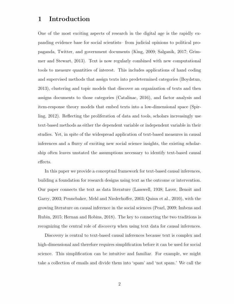
Building on the split sample approach to obtain and apply g, we explain our
suggested procedure (Figure 1) and then apply it to two specific examples: text as
the dependent variable and the text as the independent variable. In Appendix A.3
we provide a verbal description of Figure 1.
To introduce this procedure our paper proceeds as follows. In Section 2 we
provide a definition of g and describe the central role that it plays in text analysis.
4
Figure 1: Our Procedure for Text-Based Causal Inferences
Make Train/Test Split
Replicate
Suggest Next Experiment
Validate g
Estimate Effects
Test Set
Collect Documentsand Responses
Validate g
Discover g
Finalize g
Label g
Training Set
Section 3 discusses the core identification and estimation concerns that complicate
the use of g in a causal inference setting. Having described the problem, in Section 4
explains why sample splitting is a solution, describing how it works, how it addresses
the core problems we raise, and the trade-offs in its use. We also defer discussion
of prior work until this section so that we can show how our work connects to a
long-tradition of sample-splitting approaches in machine learning and more recently
in causal inference. In Section 5, we illustrate our approach using applications in two
settings: text as outcome and text as treatment. Section 6 concludes and an online
appendix provides additional technical details, proofs of key claims, and details on
statistical methods used in our applications.
2 The Central Role of g, The Codebook Function
The central problems that we address stem from the need to compress text data to
facilitate causal inference. The codebook function, g, compresses high-dimensional
5

text to a low-dimensional measure used for the treatment or outcome. In this section
we explain why g is essential, how to obtain g, and how to evaluate candidate g’s.
2.1 What is g and why do we need it?
The codebook function, g, is essential because the text is typically not usable for
social science inference in its raw form. Social scientists are often interested in some
emergent property of the text—such as the topic that is discussed, the sentiment
expressed, or the ideological position taken. Documents are high-dimensional, com-
plicated, and sparse. The result is that distinct blocks of text can convey similar
topics or sentiment. Reducing the dimensions of the text allows us to group texts
and make inferences from our data.
Suppose we are interested in understanding how candidate biographies influence
the popularity of a candidate. Each biography is unique, so we cannot estimate
the effect of any individual biography on a candidate’s popularity. Instead, we
are interested in some latent property of the text’s effect on the popularity of the
candidate, such as occupational background. In this example g might compress the
text of the biography into an indicator of whether the candidate is a lawyer. The
analyst could define g in numerous ways including hand-coding. g could also be
defined automatically from the text, by looking for the presence or absence of the
word “lawyer”, or a group of words or phrases that convey that someone has a legal
background, such as “JD”, “attorney”, and “law school”. Being a lawyer is just
one latent feature in the text. Different g’s might measure if a candidate held prior
office, went to college, or served in the military.
Our most consequential decision about g is the space we compress the text into.
Options for this space could include discrete categories, proportions, or continu-
ous variables (like ideal point estimates). We will call the lower-dimensional space
Z. Typically these low-dimensional representations are then given a label for inter-
pretation. For example, we might use g to bin social media posts into “positive,”
6

“negative,” or “neutral,” or, put portions of documents into topics that we label
“Sports,” “Weather,” or “Politics.”
Social scientists working on text as data have adopted this compression approach,
although the low-dimensional representation is often only implicit (Laver, Benoit
and Garry, 2003; Grimmer, Messing and Westwood, 2012; Spirling, 2012; Catalinac,
2016). We can also think of g as the codebook function because it plays the role
of a codebook in a manual content analysis, describing a procedure for organizing
the researcher’s texts in some systematic way. g takes on a central role because it
connects the raw text to the underlying property that the researcher cares about.
While applied work on measurement often describes the categories under study,
discussion of the implications of g as an object of interest is rare. Nevertheless, g is
always implicitly present in any systematic analysis of text—any instance where a
set of documents is placed into a common set of categories or is assigned a common
set of properties. Once a researcher decides on and estimates g, then text is usually
ready to be used in statistical analysis.
2.2 Discovering g
While g is necessary to make causal inference, rarely is it determined exactly from
a theory or prior research. Even in manual content analysis (Krippendorff, 2004;
Neuendorf, 2016), researchers typically read at least a portion of the documents
to write a codebook that determines how coders should put documents into the
categories of interest. More recently, a wide array of machine learning methods are
used to discover g from the data (Blei, Ng and Jordan, 2003; Hopkins and King,
2010). These newly discovered categories can help shape research questions, identify
powerful textual interventions, and capture text-based outcomes.
In spite of its central role across forms of text analysis, social scientists rarely
discuss the process of discovery that lead to a particular codebook. In practice,
these coding schemes are developed through iteration between coding rules and the
7

documents to be coded. We raise two main points about the discovery of g that
apply regardless of the methodology applied.
1) We can (and often do) learn g from the data. There are three strategies
for learning g from the data. First, we could read a sample of text. In manual
content analysis, g often relies on some familiarity with the text or reading a sample
of documents to decide how the text should map into categories. Second, we could
use a method to classify texts into categories using hand coded examples for training.
Supervised methods, which are conceptually similar to manual content analysis, use
statistical and algorithmic methods attempting to estimate the best g from hand
coded or otherwise labeled documents. Last, unsupervised learning discovers a low-
dimensional representation and assigns documents to that representation.
2) There is no single correct g. Regardless of the methods used in discovery,
the analyst chooses a g on the basis of their theoretical question of interest. Dif-
ferent theories imply different organizations of the text and, therefore, different g’s.
However, we can and should evaluate g once we have defined a question of interest.
Given a particular function and a particular purpose, we can label the identified
latent features, the scales measured, and the classification accuracy. The post hoc
validation of g provides clarity for both the researcher and the reader to correctly in-
terpret the underlying latent features (Grimmer and Stewart, 2013). Our goal in the
validation is to ensure that the interpretation implicit in our theoretical argument
arises from and corresponds with the mapping in our chosen g.
2.3 Finalizing g
Although there is no application-independent correct g, once we have a question
of interest, there are properties of g that are useful: interpretability, theoretical
interest, label fidelity, and tractability.
8

Property 1: Interpretability First, g should be interpretable. To claim that
a measure is theoretically interesting, we have to interpret it. Interpretability is
research and text specific, but our articles must communicate to the reader what
the measure in a specific study is capturing. This is particularly important for g’s
discovered from text data, which are based on underlying covariances in the data
and thus will not necessarily be interpretable.
Property 2: Theoretical Interest The codebook function should also create
measures of theoretical interest. We want to find low-dimensional representations
of text that operationalize concepts from a theory and identify causal effects that
test observable implications of the theory. Ideally, we would like to focus on large
magnitude causal effects. All else equal, larger effects help us to explain more of the
behavior of theoretical interest.
Property 3: Fidelity We also want to choose functions with high fidelity between
the label we give to the components of g and the text it is compressing. Establishing
fidelity involves producing evidence that the latent variable z accurately captures
the property implied by the label. This is a common exercise in the social sciences;
there is always an implicit mapping between the labels we use for our variables and
the reality of what our labels measure. For text analysis, we think of maximizing
label fidelity as minimizing the surprise that a reader would have in going from the
label to reading the text. Fidelity is closely connected to the literature on validity
in measurement and manual content analysis (see e.g., Grimmer and Stewart, 2013;
Quinn et al., 2010; Krippendorff, 2004).
Property 4: Tractable Finally, we want the development and deployment of g
to be tractable. In the context of manual content analysis this means the codebook
can be applied accurately and reliably by human coders and that the number of
documents to be coded is feasible for the resources available. In the case of learning
9

g statistically, tractability implies that we have a model which can be estimated using
reasonable computational resources and that it is able to learn a useful representation
with the number of documents we possess.
There is an inherent tension between the four properties. This is most acute with
the tension between theoretical interest and label fidelity. It is often tempting to
assign a very general label even though g is more specific. This increases theoretical
relevance, but lowers fidelity. The consequence can be research that is more difficult
to replicate. Alternatively, we might have a g that coincides with a label because it
increases the chances that our result can be replicated. But this could reduce the
theoretical interest.
The analog of g lurks in every research design, including those that use standard
data. Invariably when making an argument the researcher needs to find empirical
surrogates or operationalized the concepts in her theoretical argument. For example,
every time a researcher uses gross domestic product (GDP) as a stand-in for the size
of the economy, she is projecting a high-dimensional and complicated phenomenon—
the economy—into a lower-dimensional and more tractable variable—GDP. The
causal estimand is defined in terms of its effect on GDP, but the theoretical argument
is made about the size of the economy. While there is no correct measure to use
for the economy, the reader can and should still interrogate the degree to which
the chosen measure appropriately captures the broader theoretical concept that the
researcher wants to speak to.
3 The Problem of Causal Inference with g
Text is high-dimensional, so we use the codebook function, g, to learn a low-
dimensional representation to make inferences. But using g to compress text intro-
duces new problems for causal inference. In this section we explain how g facilitates
10

causal inference with text and then characterize the problems it creates.1 In Sec-
tion 3.1 we place g in the traditional causal inference setting. Section 3.2 explains
how the use of g leads to the problems of an analyst induced SUTVA violation and
overfitting.
3.1 Causal inference with g
To begin, we review potential outcomes notation and assumptions used when there is
no text or dimensionality reduction and we are analyzing a unidimensional treatment
and outcome (Imbens and Rubin, 2015). Denote our dependent variable for each
unit i (i ∈ 1, 2, . . . , N) with Yi, the treatment condition for unit i will be Ti. We
define the space of all possible outcomes as Y and the space of all possible treatments
as T . When the treatment is binary we refer to Yi(1) as the potential outcome for
unit i under treatment and Yi(0) as the potential outcome under control and the
individual causal effect (ICE) for unit i is given by ICEi = Yi(1) − Yi(0). Our
typical estimand is some function of the individual causal effects such as the average
treatment effect (ATE), E[Yi(1)− Yi(0)].
To identify the average treatment effect using a randomized experiment we
make three key assumptions. First, we assume that the response depends only on
the assigned treatment, often called the Stable Unit Treatment Value Assumption
(SUTVA). Specifically:
Assumption 1 (SUTVA). For all individuals i, Yi(T ) = Yi(Ti).
Second, we will assume that our treatment is randomly assigned:
Assumption 2 (Ignorability). Yi(t) ⊥⊥ Ti
Third,we will assume that every treatment has a chance of being seen:
1At a technical level we can think of an experiment with the process of discovery as a form ofdata-adaptive estimation (van der Laan, Hubbard and Pajouh, 2013), a framework which originatesfrom biostatistics and describes circumstances where our target estimation is not fixed in advance.
11

Assumption 3 (Positivity). Pr(Ti = t) > 0 for t ∈ T .
The second and third assumptions are guaranteed by proper randomization of the
experiment whereas the first is an assumption that is generally understood to mean
that there is no interference between units and no hidden values of treatment. For
each observation we observe only a single potential outcome corresponding to the
realized treatment.
Building off of this notation, we can introduce mathematical notation to cover
high-dimensional text and the low-dimensional representation of texts derived from g
that we will use for our inferences. We start by extending our notation to cover multi-
dimensional outcomes, Y i, and multi-dimensional treatments, T i. We will suppose,
for now, that we have already determined g, the codebook function. Recall g is
applicable regardless of whether the coding is done by a machine learning algorithm,
a team of undergraduate research assistants or an expert with decades of experience.
We write the set of possible values for the mapped text as Z with a subscript to
indicate if it is the dependent variable or treatment. We denote the realized values
of the low-dimensional representation for unit i as zi (i = 1, . . . , N). We suppose
that when the outcome is text g : Y → ZY and g(Y i) = zi, and when the treatment
is text g : T → ZT and g(T i) = zi. The set Z is a lower-dimensional representation
of the text and can take on a variety of forms depending upon the study of interest.
For example, if we are hand coding our documents into two mutually-exclusive and
exhaustive categories, then Z is {0, 1}. If we are using a mixed-membership topic
model to measure the prevalence of K topics as our dependent variable, then Z is
a K − 1 dimensional simplex. And if we are using texts as a treatment, we might
suppose that Z is the set of K binary feature vectors, representing the presence or
absence of an underlying treatment (see Appendix A.6.2 for the reason we prefer
binary treatments, though continuous treatments also fit within our framework).
There are numerous other types of g that we might use—including latent scales,
dictionary-based counts of terms, or crowd-sourced measures of content. The only
12

requirement for g is that it is a function.
We next use g to write our causal quantity of interest in terms of the low-
dimensional representation. To make this concrete, consider a case where we have
a binary non-text treatment and a text-based outcome (we consider other causal
estimands below). Suppose we hand code each document into one of K categories
such that for unit i we can write the coded text under treatment as g(Y i(1)) = zi(1).
We can then define the average treatment effect for category k to be:
ATEk = E[g(Y i(1))k − g(Y i(0))k] (3.1)
= E[zi,k(1)− zi,k(0)]
where zi,k(1) indicates the value of the k-th category, for unit i, under treatment.
3.2 The Problems: Identification and Overfitting
Equation 3.1 supposes that we already have a g in hand. As we mentioned above,
g is often discovered by interacting with some of the data, either by reading or
through machine learning. To describe this problem more clearly, we denote the
set of documents considered in development of g as J and write gJ to indicate
the dependence of g on the documents. Problems of identification and estimation
arise where the set of documents used to develop g, J , overlaps with the set of
documents used in estimation which we will call I. There are two broad concerns:
an identification problem arising from an Analyst Induced SUTVA Violation (AISV)
and an estimation problem with overfitting.
3.2.1 Identification concerns: Analyst Induced SUTVA Violations
If Assumption 1 holds then each observation’s response does not depend on other
units’ treatment status. But even when Assumption 1 holds, when we discover
gJ , we can create a dependence across observations in J because the particular
13

randomization may affect the gJ we estimate. This violation occurs because the
treatment vector T J – the treatment assignments for all documents J– affects the g
that we obtain, inducing dependence across all observations in J . If we then try to
use the documents in J for estimation of the effect, we have violated SUTVA. This
violation is induced by the analyst in the process of discovering g, which is why we
call it an Analyst induced violation. Appendix A.1.3 provides a formal definition of
AISV.
To see how the AISV works in practice, consider a stylized experiment on four
units with a dichotomous intervention (treatment/control) and a text-based out-
come. We might imagine potential outcomes that have a simple relationship between
treatment and the text-based outcome such as the one shown in Table 1. Treated
units talk about Candidate Morals and Polarization and control units talk about
Taxes and Immigration.
Treated ControlPerson 1 Candidate Morals TaxesPerson 2 Candidate Morals TaxesPerson 3 Polarization ImmigrationPerson 4 Polarization Immigration
Table 1: A stylized experiment indicating the potential outcomes of a textual re-sponse.
Using Table 1 we can imagine the properties of an estimator applied to this
text-based experiment as we re randomize. Suppose that for each randomization we
decide on both the form of g and estimate the treatment effect given g. For example,
consider if we observe the treatment vector (1,1,0,0), we would observe only two of
the four categories: morals and immigration. A reasonable g might compress the
text based responses to two variables: an indicator variable for discussing morals
and an indicator variable for discussing immigration. If we randomize again and
then we get (1,0, 1, 0) we observe all four categories. In this case, g might map the
text based responses to a four-element long vector, with an indicator for whether
14

each distinct category is discussed in the response. Under a third randomization
(0,0,1,1) we are back to only two categories: taxes and polarization; so g might
be two bivariate indicator variables, with the categories corresponding to whether
someone discussed taxes or not or polarization or not.
As we randomize we estimate new g’s with different categories. This lack of cat-
egory stability complicates our ability to analyze our estimators as we traditionally
do, using a framework based on re-randomization. We take this category and classi-
fication stability for granted in standard experiments because categories are defined
and fixed before the experiment. But when we estimate categories from data the
discovered g depends on the randomization and therefore dependence between units
is induced by the analyst. And even if we fix the categories, as we might do with a
supervised model, different randomizations may lead to different rules for assigning
documents to categories, leading to a lack of classification stability. If, however, we
fix g before estimating the effects, the problem is solved.
3.2.2 Estimation concerns: Overfitting
Even if we assume away the AISV, estimating g means that researchers might overfit :
discover effects that are present in a particular sample but not in the population.
This is a particular risk when researchers are searching over different g’s to find those
that best meet the criteria of interpretability, interest, fidelity and tractability. The
overfitting problem is particularly acute when a researcher is fishing — searching
over g’s to obtain statistical significance or estimates that satisfy a related criterion.
But overfitting can occur even if researchers are conducting data analysis without
ill-intentions. This happens because following best practice with almost all available
text as data methods requires some iteration. With hand coding iteration occurs
to refine the codebook, with supervised models it occurs when we refine a classifier,
and with unsupervised methods it happens as we adjust parameters to examine new
organizations.
15

Fishing and overfitting are a problem in all experimental designs and not just
those with text. The problem of respecifying g until finding a significant result is
analogous to the problem of researchers recoding variables or ignoring conditions
in an experiment, which can lead to false-positive results. (Simmons, Nelson and
Simonsohn, 2011).The problem with text-based inferences is heightened because
texts are much more flexible than other types of variables, creating a much wider
range of potential g’s. This wider range increases the risk of overfitting, even amongst
well-intentioned analysts. Overfitting is also likely in texts because it is so easy to
justify a particular g after the fact – the human brain is well-equipped to identify
and justify a pattern in a low-dimensional representation of text, even if that pattern
emerges merely out of randomness. This means that validation steps alone may be
insufficient safeguard against overfitting, even though texts provide a rich set of
material to validate the content.
4 A Train/Test Split Procedure for Valid Causal
Inference with Text
To address the identification issues caused by the AISV and the estimation challenges
of overfitting, we must break the dependence between the discovery of g and the
estimation of the causal effect. The most straightforward approach is to define
g before looking at the documents. Defining the categories beforehand, however,
limits our coding scheme, excluding information about the language used in the
experiment’s interventions or what units said in response to a treatment. If we
define our codebook before seeing text we will miss important concepts and have a
poorer measure of key theoretical concepts.
We could also assume the problem away. Specifically, to eliminate the AISV it is
sufficient to assume that the codebook that we obtain is invariant to randomization.
Take for example the text as outcome case; if over different randomizations of the
16

treatment the g we learned does not change, we don’t have an AISV. We define a
formal version of this assumption in Appendix A.1.4.
Our preferred procedure is to explicitly separate the creation of g and the esti-
mation of treatment effects. This procedure avoids the AISV and provides a natural
check against overfitting. To explicitly separate the creation of the codebook and its
application to estimate effects, we randomly divide our data into a training set and
a test set. Specifically, we randomly create a set of units in a training set denoted
by the indices J and a non-overlapping test set denoted by the indices I. We use
only the training set to estimate the gJ function and then discard it. We then use
the test set exclusively to estimate the causal effect on the documents in I.
This division between the training and test set addresses both the identification
and estimation problems. It avoids the AISV in the test set because the function g
does not depend on the randomization in the test set, so that each test set unit’s
response depends only on its assigned treatment status. There is still a dependence
on the training set observations and their treatment assignment. This, however, is
analogous to the analyst shaping the object of inquiry or creating a codebook after
a pre-test. With the AISV addressed, it is now possible to define key properties of
the estimator, like bias or consistency.
The sample split also addresses the concerns about overfitting. The analyst can
explore in the training set as much as she likes, but, because findings are verified in
a test set that is only accessed once, she is incentivized to find a robust underlying
pattern. Patterns in the training set which are due to idiosyncratic noise are highly
unlikely to also arise in the test set which helps assure the analyst that patterns which
are confirmed by the separate test set will be replicable in further experiments. By
locking g into place in the training set, the properties of the tests in the test set
do not depend upon the number of different g’s considered in the training set. In
practice, we find splitting the sample ensures that we are able to consider several
models to find the g that best captures the data and aligns with our theoretical
17

quantity of interest without worrying about accidentally p-hacking.
With the reason for sample splitting established, we first describe our final esti-
mands for the text as outcome and text as treatment cases (Sections 4.1 and 4.2).
We then describe the pragmatic steps we suggest to take to implement a train/test
split (Section 4.3). Then in Section 4.4, we discuss the tradeoffs in using a split
sample approach. Having described our strategy, in Section 4.5, we connect our
approach to existing prior work before demonstrating how it works in two different
applications (Section 5).
4.1 Text as outcome
The text as outcome setting is straightforward. The particular g that the analyst
chooses defines the categories of the outcome from which the estimand will be de-
fined. Our goal is to obtain a consistent (and preferably unbiased) estimator for
the ATE (or other causal quantities of interest) assuming a particular g. Using
Assumptions 1-3, a consistent estimator will be:
ATE =∑i∈I
I(Ti = 1)gJ(Y i(1))∑i∈I I(Ti = 1)
−∑i∈I
I(Ti = 0)gJ(Y i(0))∑i∈I I(Ti = 0)
When g is fixed before documents I are examined, we can essentially treat the
mapped outcome gJ(Y I) as an observed variable.2 Appendix A.1.2 gives an identi-
fication proof.
4.2 Text as treatment
Text may also be the treatment in an experiment. For example, we may ask in-
dividuals to read a candidate’s biography and then evaluate how the candidate’s
2It is still important to verify that the mapped variable is capturing what you care about theunderlying text. Ultimately this is not any different than ensuring that a chosen outcome for anexperiment captures the phenomenon of interest to the researcher.
18

favorability on a scale of 0 to 100. The treatment, T i, is the text description of
the candidate assigned to the respondents. The potential outcomes Yi(T i) describes
respondent i’s rating of the candidate under the treatment assigned to respondent
i.
While we could compare two completely separate candidate descriptions, social
scientists are almost always interested in how some underlying feature of a document
affects responses—that is the researcher is interested in estimating how an aspect or
latent value of the text influences the outcome.3 For example, the researcher might
be interested in whether including military service in the description has an impact
on the respondents’ ratings of the candidate. Military service is a latent variable
– there are many ways that the text could describe military service that all would
count as the inclusion of military service and many ways that the text could omit
military service that all would count as the absence of the latent variable. The
researcher might assign 100 different candidate descriptions, some which mention
the candidate’s military service and some which do not. In this case, the treatment
of interest is Zi = g(Ti) which maps the treatment text to an indicator variable that
indicates whether or not the text contains a description of the candidate’s military
service. To estimate the impact of a binary treatment, we could use the estimator:
ATE =∑i∈I
I(Zi = gJ(T i) = 1)Yi(1))∑i∈I I(Zi = gJ(T i) = 1)
−∑i∈I
I(Zi = gJ(T i) = 0)Yi(0))∑i∈I I(Zi = gJ(T i) = 0)
With text as treatment, we may be interested in more than just one latent treat-
ment. The presence of multiple latent treatments requires different causal estimands
and enables us to ask different questions about how features of the text affect re-
sponses. For example, we can learn the marginal effect of military service and how
3This distinguishes our framework from A/B tests commonly found in industry settings whichevaluate different blocks of text without attempting to understand why there are differences acrossthe texts.
19

military service interacts with other features of the candidate’s background—such
as occupation or family life. Typically with multidimensional treatments we are
interested in the effect of one treatment holding all others constant. This compli-
cates the use of topic models which suppose Z is a simplex (all topic proportions are
non-negative and sum to one) because there is no straightforward way to change one
topic holding others constant (see Fong and Grimmer 2016 and Appendix A.6.2).
Instead we will work with g that compress the text T to a vector of K binary treat-
ments Zj ∈ Z where Z represents all 2K possible combinations of the treatments.
We could also, of course, suppose that g maps T to a set of continuous underlying
treatments, but this requires additional functional form assumptions.
The use of binary features leads naturally to the Average Marginal Component
Effect (AMCE), the causal estimand commonly used in conjoint experiments (Hain-
mueller, Hopkins and Yamamoto, 2013). The AMCE estimates the marginal effect
of one component k, averaging over the values of the other components:
AMCEk =∑Z−k
E[Y (Zk = 1,Z−k)− Y (Zk = 0,Z−k)]m(Z−k)
The AMCEk describes the average effect of component k, summed over all other
values of k, weighted by m(Z−k), or an analyst determined distribution of Z−k. The
AMCE can be thought of as an estimate of the effect of component k, averaging
over the distribution of other components in the population—therefore providing a
sense of how an intervention will matter averaging over other characteristics.
In order to discover the mapping from text to latent treatments we an additional
assumption than in the text as outcome case. This is because analysts are usually
only able to randomize at the text level, but we are interested in identifying the effect
of latent treatments we are unable to manipulate directly. Consequently, we need
to make an additional assumption beyond the three mentioned above in Section 3.1
20

(SUTVA, Ignorability and Positivity4).The Sufficiency Assumption states that our
g captures all the information relevant to the response in T is contained in Z
Fong and Grimmer (2018) shows that for sufficiency to hold for any individual
the response to two documents with the same latent feature representation might
differ, but on average over individuals the responses are the same. Mathematically,
it is written as:5
Assumption 4 (Sufficiency). For all T and T′
such that g(T ) = g(T′) then
E[Yi(g(T ))] = E[Yi(g(T′))].
Fong and Grimmer (2018) shows that this assumption is equivalent to supposing
that the components of the document that affect the response and are not included in
the latent feature representation are orthogonal to the latent feature representation.
Technically, we can define εi(T ) = Yi(T ) − Yi(g(T )) and then this more general
assumption is equivalent to assuming that Ei[εi(T )] = 0 for all T . Fong and Grimmer
(2016) and Fong and Grimmer (2018) provide an identification proof.
4.3 Procedure
In this section we discuss the general procedure for implementing the train/test split
to estimate the above quantities of interest. This procedure follows the schematic
in Figure 1. Considerations specific to treatment or outcome are deferred to Ap-
pendix A.5 and Appendix A.6.
4To address the multidimensional treatments, the positivity assumption becomes the commonsupport assumption which states that all combinations of treatments have non-zero probabilityf(Zi) > 0 for all Zi ∈ Range g(·).
5Fong and Grimmer (2016) present a stronger and more intuitive version. Fong and Grimmer(2016) show that sufficiency holds if Yi(T i) = Yi(g(T i)) for all documents and for all respondents.In words, this assumption requires that the potential outcome response to the text be identicalto the potential outcome response to all documents with the same latent feature representation.This assumption is strong because it requires that there is no other information contained in thetext that matters for the response beyond what is contained in the latent feature representation.In our running example about military service, this would mean that the inclusion or exclusionof military service is the only aspect relevant to the effect of the document on the individual’srating. Particularly for text, we could imagine that this assumption could easily be violated. Ifboth versions of the treatment contain “The candidate served in the military”, but one also adds“The candidate was dishonorably discharged” we might expect that this additional text added inaddition to Z may be relevant to the responses.
21

4.3.1 Splitting the sample
The first major choice that the analyst faces is how to split the sample into two
pieces: the training set and the test set. A default recommendation is to split 50%
of the documents in training and 50% in the test set. But this depends on how
the researcher evaluates the tradeoff between discovery of g and testing. Additional
documents in the training set enables learning a more complicated g or more precise
coding rules. Additional documents in the test set enable estimation of a more
precise effect. While the test set should be representative of the population that
you want to make inference about, the training set can draw on additional non-
representative documents as long as they are similar enough to the test set to aid
in learning a useful g. Finally, when taking the sample the analyst can stratify on
characteristics of interest to ensure that the split has appropriate balance between
the train and test set on those characteristics.
Once the test set is decided, the single most important rule is that the test set is
used once, solely for estimation. If the analyst revises g after looking at the test set
data, she reintroduces the AISV and risks overfitting. Setting aside test data must
be true for all features of the analysis: even preliminary steps like preprocessing
must not include the test data set. Third parties, such as survey firms and research
agencies, can be helpful in credibly setting the data aside.
4.3.2 Discover g
We use the training set and text as data methods to find a g that is interpretable,
of theoretical interest, has high label fidelity and is tractable. In this paper we use
the Structural Topic Model and the Supervised Indian Buffet Process but there are
numerous other methods that are applicable.
22

4.3.3 Validation in the training set
Validation is an important part of the text analysis process and researchers should
apply the normal process of validation to establish label fidelity. These validations
are often application-specific and draw on close reading of the texts.6 These valida-
tions should be completed in the training set as part of the process of discovering
and labeling g, before the test set is opened.
4.3.4 Before opening the test set
While obtaining g in the training set, we can refit g as often as it is useful for our
analysis. But once applied to the test set we cannot alter g further. Therefore, we
advise two final steps.
1) Take One More Look at g
Be sure g is capturing the aspect of the texts that you want to capture, assign
labels and then validate to ensure that the conceptual gap between those labels
and the representation g produces is as small as possible. While validation ap-
proaches may vary- this necessarily involves reading documents (Krippendorff,
2004; Quinn et al., 2010; Grimmer and Stewart, 2013). It is helpful to fix a set
of human assigned labels, example documents and automated keyword labels
in advance to avoid subtle influence from the test set.
2) Fix Your Evaluation Plan
While we focus on inference challenges with g, standard experimental chal-
lenges remain. Here we can draw from the established literature on best prac-
tices in experiments (Gerber and Green, 2012) potentially including a pre-
analysis plan (Humphreys, Sanchez de la Sierra and Van der Windt, 2013).
This can include multiple-testing and false-discovery rate corrections.
6See Grimmer and Stewart (2013) for more detail on types of validation and the stm package(Roberts, Stewart and Tingley, 2017) for tools designed to assist with validation.
23

4.3.5 Applying g and estimating causal effects
Mechanically, applying g in the test set is straightforward and is essentially the
process of making a prediction for a new document. After calculating the quantities
gJ(YI) we can use standard estimators appropriate to our estimand, such as the
difference of means to estimate the average treatment effect. The appendix describes
how to apply g to new documents in both the Supervised Indian Buffet Process and
the Structural Topic Model, which we cover in our examples.
4.3.6 Validation in the test set
It is also necessary to ensure that the model fits nearly as well on the test set as it
did on the training set. When both the training and test sets are random draws from
the same population this will generally be true. But overfitting or a small sample
size can result in different model fit. The techniques used to validate the original
model can be used in the test set as well as common measures of model fit such
as log likelihood. Unlike the validation in the training set, during the validation in
the test set the analyst cannot return to make changes to the model. Nevertheless,
validation in the test set helps the analyst understand the substantive meaning of
what is being estimated and provides guidance for future experiments. Formally,
our estimand is defined in terms of the empirically discovered g in the training set.
However, invariably the analyst making a broader argument indicated by the label.
Validation in the test set verifies that label fidelity holds and that g represents the
concept in the test set of documents.
4.4 Tradeoffs
The train-test split addresses many of our concerns, but it is not without cost.
Efficiency loss is the biggest concern. In a 50/50 train-test split, half the data is
used in each phase of analysis, implying half the data is excluded from each step. At
24

the outset, it is difficult to assess how much data is necessary for either the training
or the test set. The challenge in setting the size of the test set is that the analyst
does not yet know what the outcome (or treatment) will be when the decision is
made on the size of the split. The problem in setting the size of the training set is
that we don’t know the power we need for discovery. Alternatively, we could focus
first on determining the power needed for estimation of an effect and then allocate
the remaining data for discovery. This can be effective, but it requires that we are
able to anticipate characteristics of our discovered treatment or outcome.
4.5 Prior work
Our central contribution is a framework that characterizes how to make causal infer-
ences with texts, identifies problems that arise when making those causal inferences,
and the explanation of why sample splitting addresses these challenges. There has
been comparatively little work on causal inference with latent variables. Lanza,
Coffman and Xu (2013) consider causal inference for latent class models but do not
give a formal statement of identifying assumptions or acknowledge the set of con-
cerns we identify as an analyst induced SUTVA violation. Volfovsky, Airoldi and
Rubin (2015) present a variety of estimands and estimation strategies for causal ef-
fects where the dependent variable is ordinal. They provide approaches based both
on the observed data as well as latent continuous outcomes. Volfovsky, Airoldi and
Rubin (2015) express caution about the latent variable formulation due to identifi-
cation concerns and the subsequent literature (e.g., Lu, Ding and Dasgupta, 2015)
has moved away from it. Unfortunately, many of their strategies based directly on
the observed outcomes are unavailable in the much higher dimensional setting of
text analysis. One notable exception is Gill and Hall (2015) which evaluates the
causal effect of gender on individual words in judicial decisions.
In contrast to the paucity of work on the problem we identify, our proposed
solution: sample splitting, has a long history in machine learning. There has been
25

a growing exploration of the use of train-test splits in the social sciences as well
as causal inference (Wager and Athey, 2017; Chernozhukov et al., 2017; Anderson
and Magruder, 2017). It is the natural solution to this class of problems and we
certainly do not claim to be the first to introduce the idea of train-test splits into
the area. Our approach is mostly closely related to prior work by Fafchamps and
Labonne (2017) and Anderson and Magruder (2017) which both advocate a form of
split samples to aid in discovery.
Our work is also part of a burgeoning literature on the use of machine learning
algorithms to enhance causal inference (van der Laan and Rose, 2011; Athey, 2015;
Bloniarz et al., 2016; Chernozhukov et al., 2017; Wager and Athey, 2017). Much of
this work focuses on estimating causal parameters on observed data and addressing
a common set of concerns such as estimation and inference in high-dimensional
settings, regularization bias and overfitting. Our work complements this literature by
exploring the use of latent treatments and outcomes. Many pieces in this area call for
sample splits or cross-validation for estimation and inference, providing additional
justification for our preferred approach (see e.g. Chernozhukov et al., 2017). In
Appendix A.2 we discuss the connection between our work and related work in
biostatistics.
5 Applications
We demonstrate how to make causal inferences using text in two applications: one
where text is the outcome and one where text is the treatment. Our procedure
is inherently sequential. We advocate both using a split sample design when ana-
lyzing an experiment and explicitly planning to run experiments again, in order to
accumulate knowledge. In each of the applications below we explicitly describe the
discovery process when analyzing the data. Although we use specific models, STM
for text as outcome and sIBP for text as treatment, the process we describe here is
26

general to any process for discovering g from data.
5.1 Text as outcome: an experiment on immigration
To first demonstrate how to use text as a response in a causal inference frame-
work, we apply the structural topic model to open-ended responses from a survey
experiment on immigration (Roberts et al., 2014). Specifically, we build on an ex-
periment first introduced in Cohen, Rust and Steen (2004) to assess how knowledge
about an individual’s criminal history affects respondent’s preference for punishment
and deportation. These experimental results contribute to a large literature about
Americans’ preferences about immigrants and immigration policy (see Hainmueller
and Hopkins 2014 for a review) and a literature on the punishments people view
as appropriate for crimes (Carlsmith, Darley and Robinson, 2002). Critically, in
both conditions of our experiment an individual has broken the same law, enter-
ing the country illegally, but differs solely on past criminal history. We therefore
ask how someone’s past criminal behavior affects the public’s preference for future
punishment and use the open-ended responses to gather a stated reason for that
preference.
To address this question we report the results from three iterations of a similar
experiment. With each experiment we report our procedure for choosing g and the
treatment effects in order to provide clarity and to demonstrate how the process
described in Figure 1 works in practice. The first results are based on responses ini-
tially recorded in Cohen, Rust and Steen (2004). We use this initial set of responses
to estimate an initial g and to provide baseline categories for the considerations
respondents raise when explaining why someone deserves punishment. In a second
experiment we build on Cohen, Rust and Steen (2004), but address issues in the
wording of questions, expand the set of respondents who are asked to provide an
open ended response, and update the results with contemporary data. We then run
a third experiment because we discovered our g performed poorly in the test set of
27

the second experiment. We also used that opportunity to improve small features of
the design of the experiment.
We report the results of each experiment in order to be transparent about our
research process, something we suggest that researchers do in order to avoid se-
lective reporting based on an experiment’s results. The three sets of experimental
results show that there has been surprising stability in the considerations Americans
raise when explaining their punishment preferences, though there are some new cat-
egories that emerge. There is also a consistent inclination to punish individuals who
have previously committed a crime, even though they committed the same crime as
someone without a criminal history.
5.1.1 Experiment 1
As a starting point, we conduct an analysis of the results of an experiment reported
in Cohen, Rust and Steen (2004). The survey experiment was administered in the
context of a larger study of public perceptions of the criminal justice system. The
survey was conducted in 2000 by telephone random-digit dial and includes 1,300
respondents.7
In the experiment, respondents were given two scenarios of a criminal offense. In
both the treatment and control conditions, the same crime was committed: illegal
entry to the United States. In the treatment condition, respondents were told that
the person had previously committed a violent crime and had been deported. In the
control condition, respondents were told that the person had never been imprisoned
before.
In the treatment condition, respondents were told:
“A 28-year-old single man, a citizen of another country, was convicted
of illegally entering the United States. Prior to this offense, he had
7More details about the survey are available in Cohen, Rust and Steen (2002).
28
served two previous prison sentences each more than a year. One
of these previous sentences was for a violent crime and he had been
deported back to his home country.”
In the control condition, respondents were told:
“A 28-year-old single man, a citizen of another country, was convicted
of illegally entering the United States. Prior to this offense, he had
never been imprisoned before.”
Respondents were then asked a close-ended question about whether or not the
person should go to jail. If they responded that the person should not go to jail,
they were asked to respond to an open-ended question, “Why?” The key inferential
goal of the initial study was determining if a respondent believed a person should
be deported, jailed, or given some other punishment.
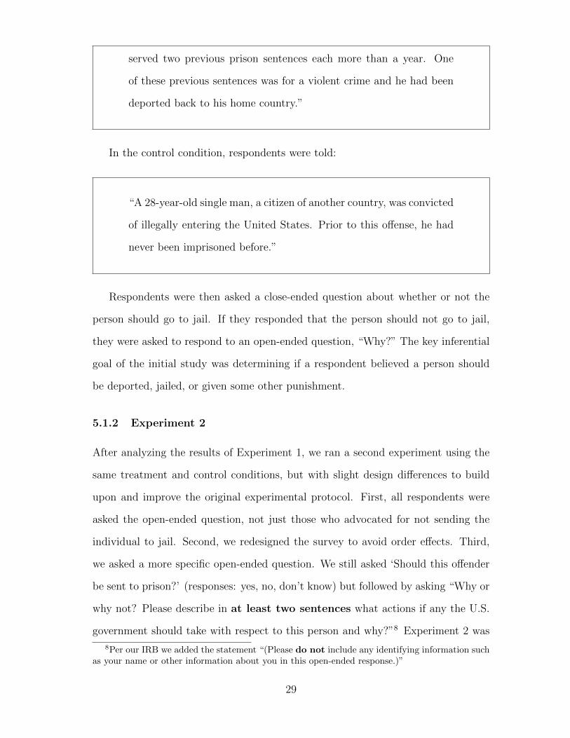
5.1.2 Experiment 2
After analyzing the results of Experiment 1, we ran a second experiment using the
same treatment and control conditions, but with slight design differences to build
upon and improve the original experimental protocol. First, all respondents were
asked the open-ended question, not just those who advocated for not sending the
individual to jail. Second, we redesigned the survey to avoid order effects. Third,
we asked a more specific open-ended question. We still asked ‘Should this offender
be sent to prison?’ (responses: yes, no, don’t know) but followed by asking “Why or
why not? Please describe in at least two sentences what actions if any the U.S.
government should take with respect to this person and why?”8 Experiment 2 was
8Per our IRB we added the statement “(Please do not include any identifying information suchas your name or other information about you in this open-ended response.)”
29

run on Mechanical Turk on July 16, 2017 with 1000 respondents.
5.1.3 Experiment 3
We expected Experiment 2 to be our last experiment, but we encountered a design
problem. After we estimated g in the training set using STM and fit it to the test
data, we realized that some of our topic labels were inaccurate. In particular, we had
attempted to label topics using three pre-determined categories: prison, deport, and
allow to stay. But the data in the second experiment suggested some new categories.
We could not simply relabel the topics in the test set, because this would eliminate
the value of the train/test split. Instead we verified the results of experiment 2 with
an additional experiment.9 Experiment 3 was run on Mechanical Turk on September
10, 2017 with 1000 respondents. To avoid labeling mistakes, two members of our
team labeled the topics independently using the training data and then compared
labels with one another to create a final set of congruent labels before applying the
g to the test set.
5.1.4 Results
In each experiment, we used equal proportions of the sample in the train and test
sets. In each experiment we fit several models in the training set before choosing a
single model that we then applied to the test set.
We include the results from all three experiments below, though because of space
constraints we put a description of topics and representative documents of Experi-
ments 1 and 2 in the Appendix. For Experiment 3, Table 2 shows the words with
the highest probability in each of 11 topics and the documents most representative
of each topic, respectively. Topics range from advocating for rehabilitation or as-
9We also took the opportunity to make a few design changes. We had previously includedan attention check which appeared after the treatment question. We moved the attention checkto before the treatment. We also had not previously used the MTurk qualification enforcing thelocation to be in the U.S. although we did in Experiment 3. Finally, we blocked workers who hadtaken the survey in Experiment 2 using the MTurkR package (Leeper, 2017).
30

sistance for remaining in the country to suggesting that the person should receive
maximal punishment.
Label Highest Probability WordsTopic 1 Limited punishment with help to stay in coun-
try, complaints about immigration systemlegal, way, immigr, danger, peopl, allow, come,countri, can, enter
Topic 2 Deport deport, think, prison, crime, alreadi, imprison,illeg, sinc, serv, time
Topic 3 Deport because of money just, send, back, countri, jail, come, prison, let,harm, money
Topic 4 Depends on the circumstances first, countri, time, came, jail, man, think, rea-son, govern, put
Topic 5 More information needed state, unit, prison, crime, immigr, illeg, take,crimin, simpli, put
Topic 6 Crime, small amount of jail time, then depor-tation
enter, countri, illeg, person, jail, deport, time,proper, imprison, determin
Topic 7 Punish to full extent of the law crime, violent, person, law, convict, commit,deport, illeg, punish, offend
Topic 8 Allow to stay, no prison, rehabilitate, probablyanother explanation
dont, crimin, think, tri, hes, offens, better,case, know, make
Topic 9 No prison, deportation deport, prison, will, person, countri, man, il-leg, serv, time, sentenc
Topic 10 Should be sent back sent, back, countri, prison, home, think, pay,origin, illeg, time
Topic 11 Repeat offender, danger to society believ, countri, violat, offend, person, law, de-port, prison, citizen, individu
Table 2: Experiment 3: Topics and highest probability words
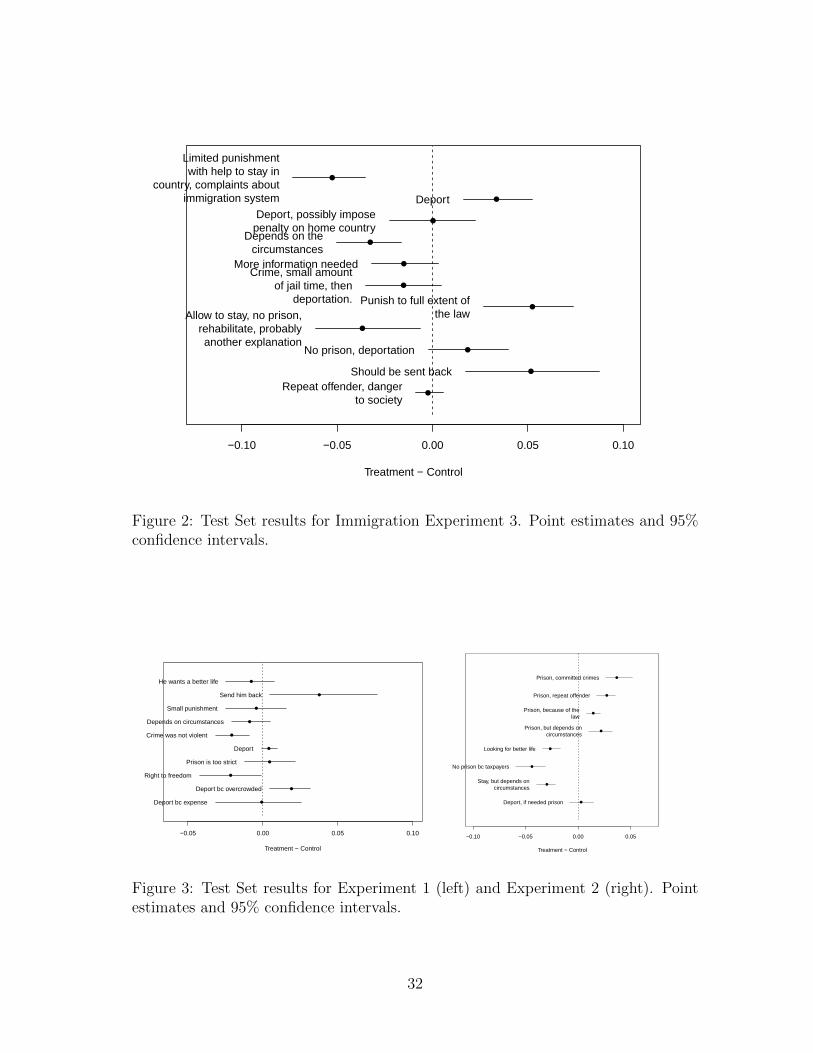
After discovering, labeling, and finalizing g in the training set, we estimated the
effect of treatment on the topics in the test set. In Figure 2 we show large impacts of
treatment on topics. Treatment (indicating that the person had a previous criminal
history) increased the amount of writing about maximal punishment, deportation,
and sending the person back to their country of origin. The control group was more
likely to advocate that the person should be able to stay in the country or that the
punishment should depend on the circumstances of the crime.
We found qualitatively similar results in Experiments 1 and 2 (Figure 3), even
though g is different in both cases and the set of people who were asked to provide
a reason is different. In each case, the description of a criminal history significantly
increases the likelihood that the respondent advocates for more severe punishment
or deportation.
Next Steps In Figure 1, we recommend concluding experiments with suggestions
for further experimentation and we do so here. Future iterations of the experiment
31
●
−0.10 −0.05 0.00 0.05 0.10
Treatment − Control
●
Limited punishmentwith help to stay in
country, complaints aboutimmigration system ●Deport
●Deport, possibly impose
penalty on home country●
Depends on thecircumstances
●More information needed
●
Crime, small amountof jail time, then
deportation.●
Punish to full extent ofthe law
●
Allow to stay, no prison,rehabilitate, probablyanother explanation
●No prison, deportation
●Should be sent back
●Repeat offender, danger
to society
Figure 2: Test Set results for Immigration Experiment 3. Point estimates and 95%confidence intervals.
●
−0.05 0.00 0.05 0.10
Treatment − Control
●He wants a better life
●Send him back
●Small punishment
●Depends on circumstances
●Crime was not violent
●Deport
●Prison is too strict
●Right to freedom
●Deport bc overcrowded
●Deport bc expense
●
−0.10 −0.05 0.00 0.05
Treatment − Control
●Prison, committed crimes
●Prison, repeat offender
●Prison, because of the
law
●Prison, but depends on
circumstances
●Looking for better life
●No prison bc taxpayers
●Stay, but depends on
circumstances
●Deport, if needed prison
Figure 3: Test Set results for Experiment 1 (left) and Experiment 2 (right). Pointestimates and 95% confidence intervals.
32

could explore two features of the treatment. First, we have only provided information
about one type of crime. It would be revealing to know how individuals respond
to crimes of differing severity. Second, we could use our existing design to estimate
heterogeneous treatment effects, which would be particularly interesting in light
of contemporary debates about how to handle undocumented immigration in the
United States.
5.2 Text as treatment: Consumer Financial Protection Bu-
reau
We turn next to examine how our framework applied to text-based treatments. We
examine the features of a complaint that causes the Consumer Financial Protection
Bureau (CFPB) to reach a timely resolution of the issue. The CFPB is a prod-
uct of Dodd-Frank legislation and is (in part) charged with offering protections to
consumers. The CFPB solicits complaints from consumers across a variety of finan-
cial products and then addresses those complaints. It also has the power to secure
payments for consumers from companies, impose fines on firms found to have acted
illegally, or both.
The CFPB is particularly compelling for our analysis because it provides a mas-
sive database on the text of the complaint from the consumer and how the company
responded. If the person filing the complaint consents, the CFPB posts the text of
the complaint in their database, along with a variety of other data about the nature
of the complaint. For example, one person filed a complaint stating that
the service representative was harsh and not listening to my ques-
tions. Attempting to collect on a debt I thought was in a grace
period ...They were aggressive and unwilling to hear it
33

and asked for remedy. The CFPB also records whether a business offers a timely
response once the CFPB raises the complaint to the business. In total, we use a
collection of 113,424 total complaints downloaded from the CFPB’s public website.
The texts are not randomly assigned to the CFPB, but we view the use of CFPB
data as still useful for demonstrating our framework. Much of the information
available to bureaucrats at the CFPB will be available in the complaint, because of
the way complaints are recorded in the CFPB data. To be clear, for the effect of
the text to be identified, we would need to assume that the texts provide all the
information for the outcome and that any remaining information is orthogonal to
the latent features of the text. We view the example of the CFPB as useful, because
it provides us a clear way to think through how this assumption could be violated.
If there are other non-textual factors that correlate with the text content, then our
estimated treatment effects will be biased. For example, if working with the CFPB
directly to resolve the complaint were important and individuals who submitted
certain kinds of complaints were less well equipped to assist the CFPB, then we
would be concerned about whether selection on observables holds. Or, there could
be demographic factors that confound the analysis. For example, minorities may
receive a slower response from CFPB bureaucrats or a more adversarial response
from financial institutions (Butler, 2014; Costa, 2017) and minorities may be more
likely to write about particular topics. While this is certainly plausible, many of the
effects that we estimate of the text are large, so they would be difficult to explain
solely through this confounding.
Our goal is to discover the treatments and estimate their effect on the probability
of a response. We discover g using the supervised Indian Buffet Process developed
for this setting in Fong and Grimmer (2016) and implemented in the texteffect
package in R (Fong, 2017). The model learns a set of latent binary features which
are predictive of both the text and the outcome. To do this, we first randomly
divide the data, placing 10% in the training set and 90% of the data in the test set.
34

Table 3: Consumer Financial Protection Bureau Latent TreatmentsNo. Automatic Keywords Manual Keyword1 payment, payments, amount, interest, balance, paid, month loan2 card, called, call, branch, money, deposit, credit card, told bank3 debt, debt collection, account, number, validation, dispute, collection debt collection4 xxxx, account, time xxxx xxxx, request, copy, received, letter detailed complaint5 payment, payments, pay, told, amount, month, called disputed payment6 loan, mortgage, modification, house foreclosure, payments mortgage7 debt, debt collection, collection, credit reporting, proof, credit report threat8 fcra, credit report, credit reporting, reporting, debt, violation, law credit report
We place more data in the test set because our large sample (≈ 11K) provides am-
ple opportunity to discover the latent-treatments in the training set and to provide
greater power when estimating effects in the test set. In the training set we apply
the sIBP to the text of the complaints and whether there was a timely response.
We use an extensive search to determine the number of features to include and the
particular model run to use. The sIBP is a nonparametric Bayesian method; based
on a user-set hyperparameter, it estimates the number of features to include in the
model, though the number estimated from a nonparametric method rarely corre-
sponds to the optimal number for a particular application. To select a final model
we then evaluate the candidate model fits utilizing a model fit statistic introduced
in Fong and Grimmer (2016) that provides a quantitative measure of model fit.
The train/test split ensures that we can refit the model several times choosing the
estimate that provides the features that provide the best substantive insights.
Once we have fit the model in the training set, we use it to the infer the treatments
in the test set. Table 3 provides the inferred latent treatments from the CFPB
complaint data. The Automatic Keywords are the words with the largest values
in the estimated latent factors for each treatment, and the manual keyword is a
phrase that we assign to each category after assessing the categories. Using these
features we can then infer their presence or absence in the treated documents and
then estimate their effect. To do this we use the regression procedure from Fong and
Grimmer (2016) and then use a bootstrap to capture uncertainty from estimation.
Figure 4 shows the effects of each latent feature on the probability of a timely
response. The black dots are point estimates and the lines are 95-percent confi-
35
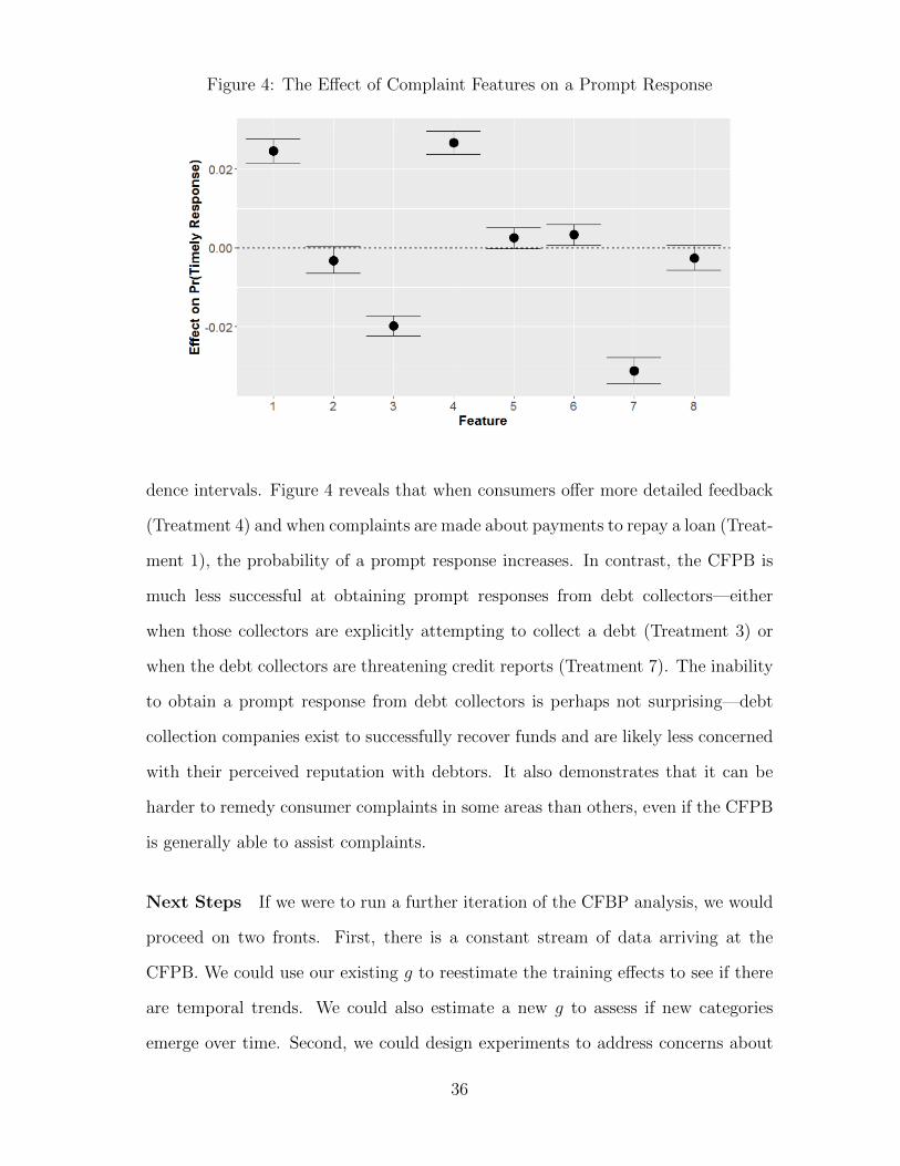
Figure 4: The Effect of Complaint Features on a Prompt Response
dence intervals. Figure 4 reveals that when consumers offer more detailed feedback
(Treatment 4) and when complaints are made about payments to repay a loan (Treat-
ment 1), the probability of a prompt response increases. In contrast, the CFPB is
much less successful at obtaining prompt responses from debt collectors—either
when those collectors are explicitly attempting to collect a debt (Treatment 3) or
when the debt collectors are threatening credit reports (Treatment 7). The inability
to obtain a prompt response from debt collectors is perhaps not surprising—debt
collection companies exist to successfully recover funds and are likely less concerned
with their perceived reputation with debtors. It also demonstrates that it can be
harder to remedy consumer complaints in some areas than others, even if the CFPB
is generally able to assist complaints.
Next Steps If we were to run a further iteration of the CFBP analysis, we would
proceed on two fronts. First, there is a constant stream of data arriving at the
CFPB. We could use our existing g to reestimate the training effects to see if there
are temporal trends. We could also estimate a new g to assess if new categories
emerge over time. Second, we could design experiments to address concerns about
36
demographic differences. For example, we could partner with individuals who are
planning to write complaints to see how their language, independent of their personal
characteristics, affects the response.
6 Conclusion
Text is inherently high-dimensional. This complexity makes it difficult to work with
text as an intervention or an outcome without some simplifying low-dimensional
representation. There are a whole host of methods in the text as data toolkit for
learning new, insightful representations of text data. Unfortunately, while these
low-dimensional representations make text comprehensible at scale, they also make
causal inference with text difficult to do well, even within an experimental context.
When we discover the mapping between the data and the quantities of interest,
the process of discovery undermines the researcher’s ability to make credible causal
inference.
In this paper we have introduced a conceptual framework for causal inference
with text, identified new problems that emerge when using text data for causal in-
ference, and then described a procedure to resolve those problems. In this conceptual
framework, we have clarified the central role of g, the codebook function, in making
the link between the high-dimensional text and our low-dimensional representation
of the treatment or outcome. In doing so we clarify two threats to causal inference:
the Analyst-induced SUTVA violation—an identification issue— and overfitting—
an estimation issue. We demonstrate that both the identification and estimation
concerns can be addressed with a simple split of the dataset into a training set
used for discovery of g and a test set used for estimation of the causal effect. More
broadly, we advocate for research designs that allow for sequential experiments that
explicitly set aside research degrees of freedom for discovery of interesting measures,
while rigorously testing relationships within experiments once these measures are
37

defined explicitly.
Our conceptual framework and procedure unifies the text as data literature with
the traditional approaches to causal inference. We have considered the text as
treatment and text as outcome, and in the future we hope to address the setting
of text as treatment and outcome. In related work, Roberts, Stewart and Nielsen
(2017) consider the text-based confounding setting. There is much more work to
be done to explore other causal designs and improvements on the work we have
presented here including optimally setting training/test splits and increasing the
efficiency of discovery methods so that they can work on even smaller data sets.
While our argument has principally been about the analysis of text data, our
work has implications for any latent representation of a treatment or outcome used
when making a causal inference. This could include latent measures common in
political science such as measures of democracy (e.g. Polity), voting behavior (e.g.
ideal points) and forms of manual content analysis. Any time a process of discovery
is necessary, we should be concerned if the discovery is completed on the same
units where the effect is estimated. In certain circumstances this process will be
unavoidable. Polity scores were developed by looking at the full population of world
democracies so there is no test set we can access, but we argue that the train/test
split should be considered in the context of the development of future measures that
require a low-dimensional representation of high-dimensional data.
What do our findings mean for existing applied work (text and otherwise)? The
AISV and overfitting raise considerable risks to replicability but it does not mean
any work not employing a train-test split is invalid. However, as estimands based
on latent constructs become more common in the social sciences, we hope to see an
increased use of the train-test split and the development of new methodologies to
enhance the process of discovery.
38

References
Anderson, Michael L and Jeremy Magruder. 2017. Split-Sample Strategies for Avoid-
ing False Discoveries. Technical report National Bureau of Economic Research.
Athey, Susan. 2015. Machine learning and causal inference for policy evaluation. In
Proceedings of the 21th ACM SIGKDD International Conference on Knowledge
Discovery and Data Mining. ACM pp. 5–6.
Blei, David M, Andrew Y Ng and Michael I Jordan. 2003. “Latent dirichlet alloca-
tion.” Journal of machine Learning research 3(Jan):993–1022.
Bloniarz, Adam, Hanzhong Liu, Cun-Hui Zhang, Jasjeet S Sekhon and Bin Yu. 2016.
“Lasso adjustments of treatment effect estimates in randomized experiments.”
Proceedings of the National Academy of Sciences 113(27):7383–7390.
Boydstun, Amber E. 2013. Making the news: Politics, the media, and agenda setting.
University of Chicago Press.
Butler, Daniel M. 2014. Representing the advantaged: How politicians reinforce
inequality. Cambridge University Press.
Carlsmith, Kevin M, John M Darley and Paul H Robinson. 2002. “Why do we
punish? Deterrence and just deserts as motives for punishment.” Journal of per-
sonality and social psychology 83(2):284.
Catalinac, Amy. 2016. “From Pork to Policy: The Rise of Programmatic Campaign-
ing in Japanese Elections.” The Journal of Politics 78(1):1–18.
Chernozhukov, Victor, Denis Chetverikov, Mert Demirer, Esther Duflo, Christian
Hansen, Whitney Newey and James Robins. 2017. “Double/debiased machine
learning for treatment and structural parameters.” The Econometrics Journal
pp. n/a–n/a.
39
Cohen, Mark A, Roland T Rust and Sara Steen. 2002. “Measuring public perceptions
of appropriate prison sentences: Report to National Institute of Justice.” NCJ
Report (199365).
Cohen, Mark A, Roland T Rust and Sara Steen. 2004. “Measuring perceptions of
appropriate prison sentences in the United States, 2000. ICPSR version. Nashville,
TN: Vanderbilt University [producer], 2000.” Ann Arbor, MI: Inter-university
Consortium for Political and Social Research.[distributor] .
Costa, Mia. 2017. “How Responsive are Political Elites? A Meta-Analysis of Experi-
ments on Public Officials.” Journal of Experimental Political Science 4(3):241–254.
Fafchamps, Marcel and Julien Labonne. 2017. “Using Split Samples to Improve
Inference on Causal Effects.” Political Analysis 25(4):465–482.
Fong, Christian. 2017. texteffect: Discovering Latent Treatments in Text Corpora
and Estimating Their Causal Effects. R package version 0.1.
Fong, Christian and Justin Grimmer. 2016. Discovery of Treatments from Text
Corpora. In Association of Computational Linguistics.
Fong, Christian and Justin Grimmer. 2018. “Exploratory and Confirmatory Causal
Inference for High Dimensional Interventions.”.
Gerber, Alan S and Donald P Green. 2012. Field experiments: Design, analysis,
and interpretation. WW Norton.
Gill, Michael and Andrew B Hall. 2015. “How Judicial Identity Changes The Text
Of Legal Rulings.”.
Grimmer, Justin and Brandon M Stewart. 2013. “Text as data: The promise and pit-
falls of automatic content analysis methods for political texts.” Political analysis
21(3):267–297.
40
Grimmer, Justin, Solomon Messing and Sean J Westwood. 2012. “How words and
money cultivate a personal vote: The effect of legislator credit claiming on con-
stituent credit allocation.” American Political Science Review 106(4):703–719.
Hainmueller, Jens and Daniel J Hopkins. 2014. “Public Attitudes Toward Immigra-
tion.” Annual Review of Political Science 17:225–249.
Hainmueller, Jens, Daniel J Hopkins and Teppei Yamamoto. 2013. “Causal inference
in conjoint analysis: Understanding multidimensional choices via stated preference
experiments.” Political Analysis 22(1):1–30.
Hernan, Miguel A and James M Robins. 2018. Causal inference. CRC Boca Raton,
FL:.
Hopkins, Daniel J and Gary King. 2010. “A method of automated nonparamet-
ric content analysis for social science.” American Journal of Political Science
54(1):229–247.
Humphreys, Macartan, Raul Sanchez de la Sierra and Peter Van der Windt. 2013.
“Fishing, commitment, and communication: A proposal for comprehensive non-
binding research registration.” Political Analysis 21(1):1–20.
Imbens, Guido W and Donald B Rubin. 2015. Causal inference in statistics, social,
and biomedical sciences. Cambridge University Press.
King, Gary. 2009. The Changing Evidence Base of Social Science Research. New
York: Routledge Press.
Krippendorff, Klaus. 2004. Content analysis: An introduction to its methodology.
Sage.
Lanza, Stephanie T, Donna L Coffman and Shu Xu. 2013. “Causal inference in
latent class analysis.” Structural equation modeling: a multidisciplinary journal
20(3):361–383.
41

Lasswell, Harold Dwight. 1938. “Propaganda technique in the world war.”.
Laver, Michael, Kenneth Benoit and John Garry. 2003. “Extracting policy posi-
tions from political texts using words as data.” American Political Science Review
97(2):311–331.
Leeper, Thomas J. 2017. MTurkR: Access to Amazon Mechanical Turk Requester
API via R. R package version 0.8.0.
Lu, Jiannan, Peng Ding and Tirthankar Dasgupta. 2015. “Sharp bounds of causal
effects on ordinal outcomes.” arXiv preprint arXiv:1507.01542 .
Neuendorf, Kimberly A. 2016. The content analysis guidebook. Sage.
Pearl, Judea. 2009. Causality. Cambridge university press.
Pennebaker, James W, Matthias R Mehl and Kate G Niederhoffer. 2003. “Psycho-
logical aspects of natural language use: Our words, our selves.” Annual review of
psychology 54(1):547–577.
Quinn, Kevin M, Burt L Monroe, Michael Colaresi, Michael H Crespin and
Dragomir R Radev. 2010. “How to analyze political attention with minimal as-
sumptions and costs.” American Journal of Political Science 54(1):209–228.
Roberts, Margaret E., Brandon M. Stewart and Dustin Tingley. 2017. stm: R
Package for Structural Topic Models. R package version 1.2.3.
Roberts, Margaret E, Brandon M. Stewart, Dustin Tingley, Christopher Lucas, Jet-
son Leder-Luis, Shana Kushner Gadarian, Bethany Albertson and David G Rand.
2014. “Structural Topic Models for Open-Ended Survey Responses.” American
Journal of Political Science 58(4):1064–1082.
Roberts, Margaret E, Brandon M. Stewart and Richard Nielsen. 2017. Matching
methods for high-dimensional data with applications to text. Technical report
Working paper.
42

Rubin, Donald B. 1980. “Comment on ‘Randomization analysis of experimental
data: The fisher randomization test’ by D. Basu.” Journal of the American Sta-
tistical Association 75(371):591–593.
Salganik, Matthew J. 2017. Bit by bit: social research in the digital age. Princeton
University Press.
Simmons, Joseph P, Leif D Nelson and Uri Simonsohn. 2011. “False-positive psy-
chology: Undisclosed flexibility in data collection and analysis allows presenting
anything as significant.” Psychological science 22(11):1359–1366.
Spirling, Arthur. 2012. “US treaty making with American Indians: Institutional
change and relative power, 1784–1911.” American Journal of Political Science
56(1):84–97.
Tukey, John W. 1980. “We need both exploratory and confirmatory.” The American
Statistician 34(1):23–25.
van der Laan, Mark J, Alan E Hubbard and Sara Kherad Pajouh. 2013. “Statistical
inference for data adaptive target parameters.”.
van der Laan, Mark J and Sherri Rose. 2011. Targeted learning: causal inference for
observational and experimental data. Springer Science & Business Media.
Volfovsky, Alexander, Edoardo M Airoldi and Donald B Rubin. 2015. “Causal
inference for ordinal outcomes.” arXiv preprint arXiv:1501.01234 .
Wager, Stefan and Susan Athey. 2017. “Estimation and inference of heterogeneous
treatment effects using random forests.” Journal of the American Statistical As-
sociation .
43

A Online Appendix
This appendix expands on the main paper, filling in a number of specific details.
• Section A.1 contains proofs and additional technical clarifications alluded to
in the main text.
• Section A.2 draws out additional connections to the machine learning litera-
ture.
• Section A.3 outlines the procedure and clarifies variance estimation.
• Section A.5 and Section A.6 provide details for STM and SIBP respectively.
• Section A.7 assess stability of the STM model across train and test splits.
• Section A.8 collects additional materials from the experiments reported in
Section 5.1 of the main paper.
A.1 Proofs and Technical Details
A.1.1 Estimation with a true g
It might seem natural to inquire about the properties of the estimator we use to
obtain g. In this setting, we can use the procedure to obtain g as an estimator G. If
we suppose that there is some true function g we might ask how well our estimator
G performs—in large samples does the g converge to g and in small samples how
discrepant is g compared to g?
While it is certainly useful to conceive of the estimator G, it is misguided to
suppose that there is a true g for some data set that our procedure is attempting to
reveal. To see why it is not useful to suppose there is a true function g consider a
hypothetical experiment where we examine how people respond to a knock on the
door and encouragement to vote. We might be immediately interested in whether
respondents are more likely to express a positive tone about political participation.
44

To investigate this, we might construct a g that measures the tone of open-ended
responses. But, we might also be interested in the topics that are discussed after
receiving a mobilization, or whether individuals mention privacy concerns. There
is also large variation in the ways we might examine how the particular contents
of the mobilization message might affect respondents. We might be interested in
whether messages that have a positive tone are more likely to increase turnout,
whether highlighting the threats from a different political party causes an increase
in turnout, or whether threatening the revelation of voter history to neighbors is
the most effective method of increasing turnout. This hypothetical example makes
clear that there is no “true” application-independent function for obtaining either the
dependent variable or treatment when making causal inferences from texts. Further,
the fact that we need to discover g at all implies that as the researcher we might be
unsure about what properties we want g to have—making it particularly difficult to
evaluate the estimator a priori.
A.1.2 Proof: Identifying ATE with text as dependent variable
This appendix section proves that after using the codebook function g on text as a
dependent variable the ATE is still preserved. We then weaken conditions needed
on g to identify the ATE.
We make Assumption 1-3 and we suppose that we have a codebook function g.
Without loss of generality we will suppose that the codebook function maps text into
a set of K categories with the constraint that the sum across all categories is equal
to 1. One example of this is using an STM to estimate the dependent variables from
a set of texts. Suppose further that we are interested in the effect of a dichotomous
intervention on the prevalence of the kth category. Our formal estimand of interest,
then, is:
45

ATEk = E[zi,1,k − zi,0,k].
Where zi,1,k corresponds to the prevalence of the kth category for observation i
after receiving Ti = 1.
We can see that the treatment effect is still identified by noting that after our
randomization we have
E[g(Y i(Ti = 1))|Ti = 1]− E[g(Y i(Ti = 0))|Ti = 0]
= E[zi,1,k|Ti = 1]− E[zi,0,k|Ti = 0]
= E[zi,1,k − zi,0,k] = ATEk
Where we apply the definition of g and the randomization of the treatments. Note
that for this proof to work, it is essential that g is fixed, otherwise the expectation
is undefined.
We can make a slightly weaker requirement of g and still preserve identification
of the causal effect. Specifically, the only requirement is that any potential other
g, g agrees with g for category k for all text documents, or that g(Y )k = g(Y )k
for all Y ∈ Y . This implies the other categories could be arbitrarily different,
but logically it requires that the total proportion of documents placed in the other
K − 1 categories is equal for both functions. The proof follows immediately from
the (obvious) proof above.
A.1.3 Technical Definition of AISV
In this section we offer a formal definition of the Analyst-Induced SUTVA Violation.
To formally define the AISV we rewrite g as explicitly dependent on training data:
46

both treatments T J and responses Y J . Specifically, we will write the value of gJ
for observation i that received treatment T i as g(Y (T i),Y J(T J)) where Y J(T J)
describes all respondents’ text-based responses and the vector of treatments for
everyone in the set J . Suppose now that we re-randomize treatment T′
J , such that
T i = T′
i and that T j 6= T′
j for at least one j ∈ J \ i. Further, suppose we obtain
new responses Y J(T′
J).
AISV problems emerge if gJ(Y (T i)) = g(Y (T i),Y J(T J)) 6= g(Y (T′
i),Y J(T′
J)) =
gJ(Y (T′
i)), even though Y (T i) = Y (T′
i)—in plain language, the lower dimen-
sional representation of document i is different between the two randomizations
even though the texts themselves are the same. This is particularly problematic if
we wanted to characterize the bias in estimators, or their properties in large sam-
ples. This is because expectations are taken over different treatment allocations.
And different treatment allocations, under many different procedures for obtaining
a codebook function g, imply that there are new categories of the dependent variable
or new treatments in the text.
A.1.4 Assuming the AISV Away
Formally, to assume away the AISV we would assume that gJ(Y (T i),Y J(T J)) =
gJ(Y (T′
i),Y J(T′
J)) for all T J ,T′
J and all J . However, the conditions for this sta-
bility can be surprisingly difficult to obtain (Chernozhukov et al., 2017). Assuming
AISV away also does not solve the problem of overfitting.
A.2 Further Connections to Literature
In this section we provide a further connection to the machine learning literature.
To make the connection, we compare our sequential approach to other methods
for ensuring that we avoid overfitting. One natural approach would be to adopt
a cross-fitting or cross-validation approach which has been extremely successful in
other contexts Anderson and Magruder (2017); Chernozhukov et al. (2017). In k-
47

fold cross validation the data is partitioned into k equally sized partitions. The
model is trained on all but one of these partitions (called the held-out set) and then
model is estimated on the held-out set. Then the procedure is repeated so each of
the k partitions is treated as the held-out set at least once. This forms an estimate
for every observation i where the prediction comes from a model which was not
trained on observation i. This is a powerful approach but relies on the idea that
the predictions will be comparable across observations which is true, for example, in
settings where the estimand is well-defined in advance of the split. In our setting,
though, we have two problems that preclude the use of cross validation. First, when
a human is in the loop there is not way to separate the model fitting procedures
because the human will remember the insights from the previous train-test split.
Second, because the estimand is not defined in advance of the split, every fold of the
cross-validation could result in our procedure could result in us measuring slightly
different concepts. The result is that we would have no coherent way to align the g
across the cross validation folds. Taken together, this suggests that a cross-validation
or cross-fitting strategy could only be pursued under strong assumptions about the
existence of a true g or with severe limitations on the discovery process.
A.3 Explanation of Procedure
The following steps are a road map for our procedure.
1) Collect a set of documents and split them into a training set and a test set.
Do not look at the test set.
2) Using your training set only, choose g that compresses the high-dimensional
text to a low-dimensional variable that will serve as either your treatment or
outcome. Assign labels to low-dimensional categories.
3) Validate that the chosen g accurately maps to a concept of theoretical signif-
icance for your argument.
48

4) Estimate the causal effect using the test set with the g discovered in test set.
You can only use the test set once.
5) Validate that the g worked as expected in the test set.
6) Ideally, replicate your findings in a new sample, repeating steps 1-5. If you
are unable to replicate, clarify what you would alter in the next experiment.
A.4 Uncertainty Estimation with g
Once we have applied g to our test data we can calculate confidence intervals using
usual variance estimators that capture uncertainty about our estimate given a lim-
ited sample size conditional on g. Examples in prior work tends to explicitly take the
view of g(Y) as a latent variable about which there is some additional measurement
uncertainty and advocated approaches to incorporate this additional uncertainty
into our confidence intervals (Roberts et al., 2014; Fong and Grimmer, 2016). For
example, Roberts et al. (2014) advocates a simulation approach to integrate over
the variational approximation to the posterior distribution which conditions on the
learned topic-word distribution, but accounts for the fact that the document-topic
proportion θ cannot be known with certainty for a particular document because it has
a finite length. Fong and Grimmer (2016) use a bootstrap approach which captures
measurement uncertainty both in the topic-word parameters and the document-topic
representation. While this approach is intuitively appealing, it complicates the def-
inition of g as a function because we run the risk of the same text mapping to two
different values of the latent variable (failing the vertical line test). In the interest of
simplicity we do not include this form of measurement error in this article and leave
to future work the incorporation of this uncertainty into the causal framework.
49

A.5 Structural Topic Model
The Structural Topic Model is a mixed membership model of texts related to La-
tent Dirichlet Allocation (Blei, 2012) which was developed in Roberts et al. (2014);
Roberts, Stewart and Airoldi (2016) and implemented in the stm package in R
(Roberts, Stewart and Tingley, 2017). It allows for the analyst to incorporate ob-
served document metadata which is able to affect either topical prevalence (the
amount which a topic is discussed) and topical content (the way in which a topic
is discussed). In this paper we consider the case in which a set of observed meta-
data which includes the treatment and pre-treatment covariates are allowed to affect
topic prevalence and there are no topical content covariates. Denoting the pretreat-
ment covariates for document i as X i and the scalar treatment as Ti, the generative
process can be given as:
ηi ∼ Normal(X iγX + Tiγτ ,Σ)
θi,k =exp(ηi,k)∑Kk=1 exp(ηd,k)
zi,n ∼ Categorical(θi)
wi,n ∼ Categorical(βzi,n)
Where θd is a K-dimensional vector on the simplex indicating the proportion of
the document allocated to each topic formed by applying the softmax function to
ηd a vector in RK−1 where the K-th element is fixed to zero. zi,n is a token level
latent variable containing the assignment for token n of document i. β is a K
by V dimensional matrix where each row contains the conditional probability of
seeing word v given that is about topic k. The model differs from Latent Dirichlet
Allocation in its use of a logistic normal prior distribution for the document-topic
proportions and through the ability to have that prior centered at a document-
specific location determined by the document metadata.
50

The model is estimated using partially-collapsed, non-conjugate, variational in-
ference. γ and Σ are given regularizing priors of the user’s choice and β is point
estimated. The model optimization problem is non-convex and so a careful initializa-
tion strategy is necessary (Roberts, Stewart and Tingley, 2016). Roberts, Stewart
and Tingley (2016) advocate a deterministic initialization based on the spectral
method of moments (Arora et al., 2013) which we refer to below as the spectral
initialization.
A.5.1 Obtaining and using g
In a given experiment we employ the following steps:
• Create the train-test split
• In the training set (discovery)
– explore the documents as desired using STM
– choose an estimand (including assigning and validating a label)
– Identify the mapping function g such that
θi = g(Y i, β, µi, Σ)
• In the test set (evaluation)
– Using tg, obtain our transformed outcome for each document. (see below
for details)
– Estimate treatment effects (using for example the difference of means)
– Validate model fit and label fidelity in the test set.
Application of g in STM is equivalent to predicting θi for a held-out document i.
This can be accomplished with the recently added fitNewDocuments function in the
51

stm package. In the STM model, the latent variable θi is a function of a global prior
(µ,Σ), the topic word parameters β and the observed words Wd. The token-level
latent variables Z are integrated out. We have estimated β in the train set and in
many ways this communicates what the topics substantively contain. We must also
decide how to set our priors µ and Σ.
The stm package offers three options: no prior, the covariate-specific prior and
the average prior. The ‘no prior’ setting sets µ to a vector of zeroes and Σ to be
a diagonal matrix with very large diagonals. The covariate-specific prior uses the
observed covariates in the new documents to construct the document-specific prior.
The average prior averages over the values of µ in the training set and provides a
single average prior for all documents.10
If we have used only pre-treatment covariates in the STM model we can use any
of these strategies. In our application we do include the treatment and so we cannot
use the covariate-specific prior because then the same text would yield two different
values of the outcome depending on the treatment assignment. For our application
we use the average prior. When using a version of g which is not the covariate-specific
prior, we recommend that analysts assess effects in the training set using the same
procedure as in the test set. While the effects will generally not be very different
(particularly for long documents), maintaining the same procedure should provide
a better expectation of test set behavior. For example, in our application Figure 5
compares our training set estimates using both the covariate-specific prior and the
averaged prior and compares them to the test set (which uses the averaged prior).
Using the average prior to make predictions in the training set before calculating
effect estimates gives us a better indication of what we will eventually observe in
the test set.
10More specifically we take the column means of the D by K − 1 matrix µ in the training setwhich we call µ. We then recalculate Σ as though the update had been made using the new valueof µ. The update is then Σ = Σ−
(∑d(ηd − µd)(ηd − µd)T
)+(∑
d(ηd − µd)(ηd − µd)T).
52

●
−0.10 −0.05 0.00 0.05 0.10
Treatment − Control
●He wants a better life
●Send him back
●Small punishment
●Depends on circumstances
●Crime was not violent
●Deport
●Prison is too strict
●Right to freedom
●Deport bc overcrowded
●Deport bc expense ●
Training SetTraining Set With Averaged PriorTest Set
Figure 5: Train-Test set effect comparing g using the model estimates (trainingset), the training set with averaged prior and the test set. Note that while theestimates are broadly similar, in general the training set with averaged prior is acloser approximation to what we end up seeing.
53

A.6 Supervised Indian Buffet Process
This appendix provides a brief review of additional estimands and an argument for
the use of binary features along with a model for estimating them.
A.6.1 Additional estimands
The analyst might also be interested in estimating the effect of an interaction be-
tween two components k and l. For example, the researcher might be interested if
including military service into a candidate profile has a different effect on candidate
ratings if the profile also includes that the candidate is female. This could be esti-
mated as the Average Component Interaction Effect (ACIE) (Hainmueller, Hopkins
and Yamamoto, 2013) :
ACIEk,l =
∫Z−k,−l
E[(Y (Zk = 1, Zl = 1, Z−k,−l)− Y (Zk = 1, Zl = 0, Z−k,−l))
− (Y (Zk = 0, Zl = 1, Z−k,−l)− Y (Zk = 0, Zl = 0, Z−k,−l)]m(Z−k,−m)dZ−k,−m
The ACIE will be the difference between the AMCE for military service for a
candidate description that includes information that the candidate is female and
the AMCE for military service for a candidate description that does not include this
information.
Note that the three complications from the last section also pertain to the case of
multidimensional treatments. If the mapping g between T andZ is not known before
defining and reading the treatment texts or the outcome is used in the estimation of
these mapping, then an AISV will occur. Even when using hand coding, researchers
should either use a pre-test to determine their coding scheme or use a training/test
split to first learn a coding scheme using the responses and then separately estimate
the treatment effects.
54

A.6.2 The argument for binary features
In this section we explain why we use binary features of texts in order to estimate
causal effects. A different approach to estimating the function g would be to estimate
real valued features that explain the text well, such as the principal components of
a document term matrix or some other low-dimensional embedding of the observa-
tions. Using these real valued embeddings for Z, the impact of Z on Y can be
estimated directly. Using real valued features of documents, however, causes sev-
eral problems that leads us to use binary features instead. First, many methods
for discovering real valued features incorporate information about the text, but not
the response. For example, we might use the loadings on principal components to
describe text-treatments. This can lead to the discovery of features that explain the
content of texts but do not explain the response to those texts and therefore are
not particularly useful for causal inference. This makes clear that our goal should
be to find a low-dimensional representation that explains both the texts and the
response well. Second, using real valued features requires the imposition of a strin-
gent set of functional form assumptions. This is because even flexibly estimating
the response to some continuous feature requires some guidance from a model. And
the more flexible the fit, the more data needed to credibly estimate the response
to the continuous treatment. And as the number of included factors increases, the
curse of dimensionality makes it all but impossible to fit anything other than a lin-
ear regression. Alternative approaches, such as an Indian Buffet Process (Griffiths
and Ghahramani, 2011), yield a binary feature vector about the treatments that are
present or absent in a text, but fail to include information about the responses.
Given the issue with continuous treatments and the importance of including
information about the response, we use a method that finds latent features and
observation’s binary loading on those features, which are then used to estimate
treatment effects. Fong and Grimmer (2016) create an unsupervised method for
estimating treatments from text data and the responses. They develop a supervised
55

Indian Buffet Process (sIBP) that discovers the topics within the documents that
are related to the outcome. The authors assume that the proportion of documents
in each latent feature k is πk, where πk is generated by a stick-breaking algorithm
(Doshi et al., 2009). Each document can be summarized by treatment vector Zj
where zj,k ∼ Bernoulli(πk). Note that because each individual zj,k is drawn from a
Bernoulli that a treatment document can have more than one latent feature, allowing
for multi-dimensional treatments.
The authors assume a mapping from Zi to the standardized term-document ma-
trix Xi through the D-dimensional vector Ak, where Xi ∼ MvtNormal(ZiA, σ2nID).
The latent feature vector Zi also affects the response Yi through the normal, Yi ∼
Normal(Ziβ, τ−1) where τ ∼ Gamma(a, b). Thus with the model the authors both
want to discover the latent treatments Zi and estimate their influence on the out-
come by estimating β. The authors use variational approximation to estimate these
parameters.
Fong and Grimmer (2016) apply the sIBP to the training data in order to learn
g. In the test set Fong and Grimmer (2016) use g to infer the treatments that are
present in a particular text, but alter the inference to avoid conditioning on the
dependent variable. They do this because otherwise the inferred treatments present
in the test set will depend upon the observation’s response to that text, which creates
obvious problems for causal inference.
Once the latent treatments are inferred in the test set documents, their effect
can be estimated using any procedure that might be used to analyze an experiment.
Fong and Grimmer (2016) use a simple linear regression with each of the latent
features as the regressors to estimate the effects of the treatments. More complicated
models could be used to estimate interactions or to extrapolate effects to a different
population of documents.
56

A.7 Stability Across Train-Test Splits
Our approach does not require stability of analysis across different train-test splits.
Different train-test splits might lead to different discovery phases which in turn yield
different estimands and test sets where we can evaluate that estimand. Nevertheless,
we might be slightly uncomfortable with the idea that the particular randomization
into the train-test spit yield quite different estimands (and papers) at the end of the
process. As such we wanted to evaluate the stability of the STM under different
samples of a fixed population.
In a formal sense we are interested in studying the posterior contraction rates
of the model, a problem taken up analytically in Tang et al. (2014) for the re-
lated Latent Dirichlet Allocation model. However, we are far more interested in
understanding performance in practice and whether different train-test splits lead
to substantively different topic-word distributions (β), different document-topic pro-
portions (θ) and different covariate effects. As the number of documents increase
or the topics are more sharply defined stability will improve. For this demonstra-
tion we use the Poliblog data (Eisenstein and Xing, 2010), a collection of around
13,246 posts from six different political blogs in the runup to the 2008 American
presidential election. We use this because it is readily available for use with the stm
package and is roughly representative of the document lengths that we often see in
stm applications overall. We would expect that the diversity of topics in political
blogs would make the problem harder than the more focused open-ended response
case, but the length of the documents would make it easier.
We started by estimating the model on the full set of documents with 20 topics
using the spectral initialization. We consider this to be the “truth” because the
unattainable stability ideal would be that the subsamples provide the same answer as
the full set of documents. We then choose two prominent topics to be our “outcomes”
a topic about Obama and a topic about War (particularly Iraq and Afghanistan). In
each simulation we choose the topic that most closely approximates our two chosen
57

outcomes, emphasizing that the labels ’Obama’ and ’War’ may well not be good
approximations for the topic in the subsample.
Because of the multimodality problem in topic models, instability could arise
from two sources: differences in the local mode discovered and differences in the data
observed. We investigate this by considering three different initialization strategies:
1) Cold Spectral Start
Using the spectral initialization on the subsample. This is reflective of current
practice.
2) Warm Spectral Start
Use the complete data to initialize the model. This would create an analyst-
induced SUTVA violation as it shares information from the test set. However,
it is suggestive of what might be achievable by providing more stable intial-
izations.
3) Warm Oracle Start
Use the results of the converged model on the full sample to initialize each
subsample. This is an infeasible estimator. The instability in this estimate
cannot be reduced by a better initialization strategy.
In each case we run the model on the sample sizes 100 times and plot the results
along with the ‘truth’ as defined by the full document set. Figure 6 shows the results
for the average proportion of the topic use in the corpus.
As we can see the results are reasonably stable at 5000 documents for a corpus of
this complexity and less so with 1000. The warm spectral start shows considerable
improvement for the 5000 document case suggesting that at least at this scale, we
might see substantial gains from an initialization specificly designed to be more
stable across splits. The near perfect stability of the warm oracle start for the
5000 document case suggests it is a matter of the initialization and not necessarily
58

Figure 6: Stability of θ in Simulations of Train-Test Splits on Real Data.Sample=5000 with Cold Spectral
start
0 20 40 60 80 100
−0.
050.
000.
050.
100.
15
Theta: Obama
Index
simtruediff
0 20 40 60 80 100
−0.
050.
000.
050.
100.
15
Theta: War
Index
Sample=1000 with Cold Spectral
Start
0 20 40 60 80 100
−0.
050.
000.
050.
100.
15
Theta: Obama
Index
simtruediff
0 20 40 60 80 100
−0.
050.
000.
050.
100.
15
Theta: War
Index
Sample=5000 with Warm Spectral
Start
0 20 40 60 80 100
−0.
050.
000.
050.
100.
15
Theta: Obama
Index
simtruediff
0 20 40 60 80 100
−0.
050.
000.
050.
100.
15
Theta: War
Index
Sample=1000 with Warm Spectral
Start
0 20 40 60 80 100−
0.05
0.00
0.05
0.10
0.15
Theta: Obama
Index
simtruediff
0 20 40 60 80 100
−0.
050.
000.
050.
100.
15
Theta: War
Index
Sample=5000 with Warm Oracle
Start
0 20 40 60 80 100
−0.
050.
000.
050.
100.
15
Theta: Obama
Index
simtruediff
0 20 40 60 80 100
−0.
050.
000.
050.
100.
15
Theta: War
Index
Sample=1000 with Warm Oracle
Start
0 20 40 60 80 100
−0.
050.
000.
050.
100.
15
Theta: Obama
Index
simtruediff
0 20 40 60 80 100
−0.
050.
000.
050.
100.
15
Theta: War
Index
the data itself, where for 1000 documents there is evidence that some level of the
instability is unavoidable given the model.
We can also examine the word-distributions themselves. Figure 7 shows the
proportion of mass associated with each of the top ten words in the topic (as chosen
by the full model). The horizontal tickmarks on the right show the estimate in the
full data.
Generally speaking the models correctly preserve the rank ordering of the most
prominent words in each topic, but the estimates can often be substantially in-
59

Figure 7: Stability of β in Simulations of Train-Test Splits on Real Data.Sample=5000 with Cold Spectral
Start
0 20 40 60 80 100
0.00
0.05
0.10
0.15
0.20
Beta: Obama
Split
beta
0 20 40 60 80 100
0.00
0.01
0.02
0.03
0.04
0.05
Beta: War
Split
beta
Sample=1000 with Cold Spectral
Start
0 20 40 60 80 100
0.00
0.05
0.10
0.15
0.20
Beta: Obama
Split
beta
0 20 40 60 80 100
0.00
0.01
0.02
0.03
0.04
0.05
Beta: War
Split
beta
Sample=5000 with Warm Spectral
Start
0 20 40 60 80 100
0.00
0.05
0.10
0.15
0.20
Beta: Obama
Split
beta
0 20 40 60 80 100
0.00
0.01
0.02
0.03
0.04
0.05
Beta: War
Split
beta
Sample=1000 with Warm Spectral
Start
0 20 40 60 80 1000.
000.
050.
100.
150.
20
Beta: Obama
Split
beta
0 20 40 60 80 100
0.00
0.01
0.02
0.03
0.04
0.05
Beta: War
Split
beta
Sample=5000 with Warm Oracle
Start
0 20 40 60 80 100
0.00
0.05
0.10
0.15
0.20
Beta: Obama
Split
beta
0 20 40 60 80 100
0.00
0.01
0.02
0.03
0.04
0.05
Beta: War
Split
beta
Sample=1000 with Warm Oracle
Start
0 20 40 60 80 100
0.00
0.05
0.10
0.15
0.20
Beta: Obama
Split
beta
0 20 40 60 80 100
0.00
0.01
0.02
0.03
0.04
0.05
Beta: War
Split
beta
correct. We do emphasize that there is relatively little information with which to
estimate these parameters and so we would expect to see more instability than in
the simulations for θ.
Finally we present estimates of “treatment effects.” Here we use the binary rating
variable (indicating whether the blog is liberal or conservative) as a treatment. This
is clearly not randomly assigned and we use it simply because it is a binary covariate
we would expect to influence the outcome in some way. We plot the estimate with a
95% confidence interval in Figure 8 along with the estimate in the complete dataset
60
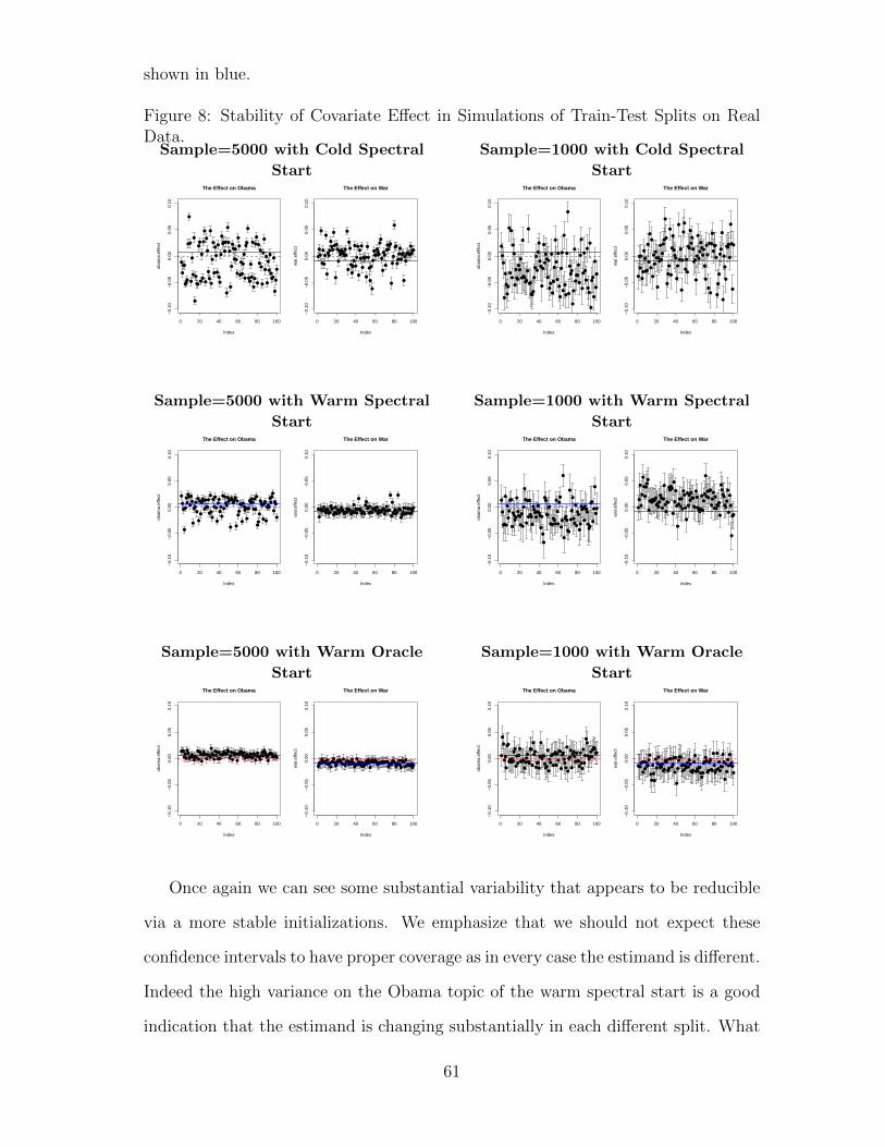
shown in blue.
Figure 8: Stability of Covariate Effect in Simulations of Train-Test Splits on RealData.
Sample=5000 with Cold Spectral
Start
●
●
●●
●●●
●
●
●
●
●
●
●
●
●
●●
●
●
●
●
●
●
●
●
●
●
●
●
●
●
●
●
●
●
●
●
●
●
●
●
●
●●
●
●
●
●
●
●
●
●
●
●
●
●
●
●
●
●
●
●
●
●
●
●
●●
●
●●
●
●
●
●
●
●
●
●
●
●
●
●
●
●
●
●
●
●
●
●
●
●
●●
●
●
●
●
0 20 40 60 80 100
−0.
10−
0.05
0.00
0.05
0.10
The Effect on Obama
Index
obam
a.ef
fect
●
●
●
●
●
●
●
●
●
●
●●
●
●
●●
●
●
●
●
●
●
●●
●●●
●
●
●
●
●
●
●
●
●
●
●
●
●
●
●
●
●
●
●
●
●●●
●
●
●
●
●
●
●
●
●
●●
●●●
●
●
●
●
●●
●
●
●
●
●●
●
●
●
●
●●
●
●
●
●
●
●●
●
●
●
●●●●
●
●●●
0 20 40 60 80 100
−0.
10−
0.05
0.00
0.05
0.10
The Effect on War
Index
war
.effe
ct
Sample=1000 with Cold Spectral
Start
●
●
●
●
●
●
●
●
●
●
●
●
●
●
●
●
●●
●
●
●
●
●
●●
●●
●
●
●●
●●●
●
●
●
●
●
●
●
●
●
●
●
●
●
●
●
●
●
●
●
●
●
●
●
●
●
●
●
●
●
●
●
●
●
●
●
●
●
●
●●
●
●
●
●
●●
●
●
●
●
●
●
●
●
●
●
●
●
●
●
●●
●
●
●
●
0 20 40 60 80 100
−0.
10−
0.05
0.00
0.05
0.10
The Effect on Obama
Index
obam
a.ef
fect
●
●
●
●
●
●
●
●
●●
●
●
●
●
●
●
●
●
●
●
●
●●
●
●
●
●
●
●
●
●
●
●
●
●
●
●
●
●●
●
●
●
●
●
●
●
●
●
●
●
●
●●
●
●
●
●
●●
●
●
●
●
●
●
●
●
●
●
●
●
●
●
●
●
●
●
●
●●
●
●
●
●
●
●
●
●
●
●
●
●●●
●
●
●
●
●
0 20 40 60 80 100
−0.
10−
0.05
0.00
0.05
0.10
The Effect on War
Index
war
.effe
ct
Sample=5000 with Warm Spectral
Start
●
●
●
●
●
●
●
●●
●
●
●
●
●●
●
●
●
●
●
●
●●●
●
●
●●
●
●
●
●
●
●
●
●
●
●
●
●
●
●
●
●
●
●
●●
●
●●
●
●●●●●
●
●
●
●
●●
●
●
●●●
●
●●
●●
●●
●
●
●
●
●●
●
●●●
●
●●
●
●●●
●
●
●
●
●
●●
●
0 20 40 60 80 100
−0.
10−
0.05
0.00
0.05
0.10
The Effect on Obama
Index
obam
a.ef
fect
●
●
●●●●●●●
●●●●
●●●
●●
●
●●●
●●●●●●●●
●●●●●●
●
●
●●
●
●
●
●●●●●●
●
●
●●
●
●
●●
●●●●
●
●●●●●
●●
●●
●
●●●
●
●
●
●●●
●●
●
●●
●●●
●
●
●
●
●●
●
●
●●●
0 20 40 60 80 100
−0.
10−
0.05
0.00
0.05
0.10
The Effect on War
Index
war
.effe
ct
Sample=1000 with Warm Spectral
Start
●
●
●●
●
●
●
●
●
●●
●
●●
●●
●
●
●●
●
●
●
●
●
●
●
●
●
●
●●
●
●●●
●
●
●
●●
●
●
●
●
●●
●●
●●
●●●
●●
●
●
●
●
●
●
●
●
●
●
●●
●
●●
●
●
●
●
●
●
●
●
●●
●
●
●●●
●
●●●
●
●●
●●
●
●
●
●
●
0 20 40 60 80 100
−0.
10−
0.05
0.00
0.05
0.10
The Effect on Obama
Index
obam
a.ef
fect
●
●
●
●
●
●
●
●
●
●
●
●
●●●●●●
●
●●●
●
●●
●
●
●
●
●
●●
●●
●●
●
●
●
●
●
●
●
●
●
●
●
●
●
●
●
●
●
●
●
●
●●
●●
●
●
●●●●
●
●
●
●
●
●
●
●
●●
●
●
●
●
●
●
●●●
●
●
●
●●
●●
●
●
●
●
●
●
●●
0 20 40 60 80 100
−0.
10−
0.05
0.00
0.05
0.10
The Effect on War
Index
war
.effe
ct
Sample=5000 with Warm Oracle
Start
●●●
●●
●
●●
●●●
●●●●●●
●
●
●●
●
●●●●
●
●●●●
●
●●
●
●
●
●
●
●
●
●●●●●●●
●●
●●
●
●
●●●●
●
●●●●●
●●
●●●●●●
●
●●
●●
●
●●
●●●
●●●
●●●●
●
●●●●●●●●●
0 20 40 60 80 100
−0.
10−
0.05
0.00
0.05
0.10
The Effect on Obama
Index
obam
a.ef
fect
●●●●
●●●●●
●
●●●
●
●●●
●●●
●●●●●●
●
●●●●●
●●●
●●●
●●
●
●●●●
●●
●●●
●●
●●
●
●●●●
●●●
●●●●●
●●●●●●
●●●●
●●●●●●●
●
●●
●●●
●
●
●●●●●●
●●
0 20 40 60 80 100
−0.
10−
0.05
0.00
0.05
0.10
The Effect on War
Index
war
.effe
ct
Sample=1000 with Warm Oracle
Start
●
●
●
●
●
●
●●
●●●●●
●●
●
●
●
●
●
●●●●
●
●
●
●
●●
●●
●
●
●●
●
●●
●
●
●
●●●
●
●●
●
●
●●
●●
●
●●
●
●
●
●●
●
●●
●
●
●
●
●
●●
●
●
●●
●
●
●
●●
●
●
●
●
●
●
●
●
●
●●●
●
●
●●●
●●
0 20 40 60 80 100
−0.
10−
0.05
0.00
0.05
0.10
The Effect on Obama
Index
obam
a.ef
fect
●●●
●●
●
●
●
●
●●
●
●
●
●
●
●
●
●
●
●
●
●●●
●
●●
●●●
●●
●●
●●
●
●
●
●
●
●
●●
●
●
●
●
●●
●
●
●
●
●●●
●
●
●●●
●●
●
●
●
●●
●
●
●●
●●
●●
●
●
●●
●
●
●
●
●●
●
●
●
●
●
●
●
●
●●●
●
0 20 40 60 80 100
−0.
10−
0.05
0.00
0.05
0.10
The Effect on War
Index
war
.effe
ct
Once again we can see some substantial variability that appears to be reducible
via a more stable initializations. We emphasize that we should not expect these
confidence intervals to have proper coverage as in every case the estimand is different.
Indeed the high variance on the Obama topic of the warm spectral start is a good
indication that the estimand is changing substantially in each different split. What
61

the relatively tight set of estimates in the two warm starts suggest is that this might
be avoidable with a different initialization.
In summary, there is a significant degree of instability across splits. Again, this
is not a problem in a technical sense as gapplied to the test set will still provide a
proper estimator of that specific estimand. What these simulations do suggest is
that further research into more stable initialization strategies might substantially
reduce the amount of instability across train-test splits.
There are several limitations to this simulation study: most notably that we
neither know the actual truth nor can we be sure what the scope conditions are
for these results to apply to other datasets. We also cannot simulate the stability
of the entire discovery process, only that a particular model is comparable across
subsamples. Hoping for stability in discovery may be quixotic as the very idea of
discovery itself may imply some level of instability.
62

A.8 Full set of experimental results for the Immigration Ex-
periment
Label Highest Probability WordsTopic 1 He wants a better life didnt, want, pay, better, life, probabl, isntTopic 2 Send him back back, countri, send, home, well, charg, troublTopic 3 Small punishment offens, reason, like, chanc, first, can, citizenTopic 4 Depends on circum-
stancescome, depend, doesnt, free, feel, law, shouldnt
Topic 5 Crime was not vio-lent
crime, commit, violent, immigr, wasnt, look,never
Topic 6 Deport deport, that, give, counti, peopl, look, guiltiTopic 7 Prison is too strict enter, anyth, right, live, realli, illeg, anybodiTopic 8 Right to freedom just, tri, get, hes, came, freedom, putTopic 9 Deport bc over-
crowdedsent, prison, think, alreadi, anoth, done, hasnt
Topic10
Deport bc expense dont, think, know, time, need, serv, crimin
Table 4: Experiment 1, Words most representative of topics.
63

Label Representative DocumentTopic 1 He wants a better life we’re the land of opportunity everybody wants a
better lifeTopic 2 Send him back send him back to his countryTopic 3 Small punishment ”it was his first offense, didn’t hurt anybody,
maybe a fine though, probation or something.that’s nice serious like murder or robbery”
Topic 4 Depends on circum-stances
it depends on reaason why he is coming into stateif he was coming to beter himself its ok if he hasa record he should be disbarred or deported
Topic 5 Crime was not vio-lent
because he didnt commit a crime that was effect-ing someone else’s individual liberties
Topic 6 Deport he should be deportedTopic 7 Prison is too strict because he didnt do anything except illegally enterTopic 8 Right to freedom Because he’s just trying to get his freedom.
Maybe he’s trying to away from a tough situa-tion/that country-maybe it’s not good for him.
Topic 9 Deport bc over-crowded
he should be sent to prison in another country ourprisons are over crowded already
Topic10
Deport bc expense because i think he shold be deported-p-i don’tthink he should be supported in our prison sys-tem and i don’t think he should be allowed toimmigrate here
Table 5: Representative documents of each topic.
Label Highest Probability WordsTopic 1 Prison, committed crimes crime, commit, violent, illeg, immigr, punish, convictTopic 2 Prison, repeat offender state, unit, offend, need, offens, enter, repeatTopic 3 Prison, because of the law law, jail, time, alreadi, come, will, priorTopic 4 Prison, but depends on cir-
cumstancesserv, prison, sentenc, one, time, know, feel
Topic 5 Looking for better life person, crimin, govern, better, life, good, stayTopic 6 No prison bc taxpayers imprison, money, believ, allow, origin, tax, taxpayTopic 7 Stay, but depends on circum-
stancesthink, illeg, enter, dont, peopl, just, man
Topic 8 Deport, if needed prison countri, deport, prison, back, sent, home, send
Table 6: Experiment 2, Words most representative of topics.
64

Label Representative DocumentTopic 1 Prison, committed crimes He committed crimes, and most importantly, violent crimes, so
should be convicted on that. I am not concerned as much withhis immigration status, although the fact that he keeps returningafter deportation should be taken into account. I am not judging hisorigin, just his crimes.
Topic 2 Prison, repeat offender Because the man is a citizen of another country. that is not mainmatter. illegaly entered the united states this is main mistake. sothat man is lock to prison
Topic 3 Prison, because of the law It’ll be the first lesson for him to obey the laws. Secondly, teach himto think before do the things.
Topic 4 Prison, but depends on cir-cumstances
I really don’t know how to judge the severity of this crime and whatan appropriate punishment would be. If someone were to sneek intoa club, ball game, or onto private property in general they wouldprobably be at least subject to trespassing charges but my guess isthis would involve only a fine and not prison time. However, thiscrime is probably more severe. If someone were to sneek onto thegrounds of the White House I think they would likely be chargedwith crimes that involve prison time however illegally entering theUnited States might be considered less sever than such a crime. Iguess I’d have to here arguments for and against before I could cometo some sort of conclusion. In general, I don’t have a strong sense ofthe harms of the crime.
Topic 5 Looking for better life He has never been in trouble before, he is obviously looking for safetyand he should be helped along the road to becoming a citizen.
Topic 6 No prison bc taxpayers His entry into the US costed the US tax payer nothing. His crime andimprisonment would cost the US tax payer thousands of dollars infood, shelter, health care, etc... for this man. It is cheaper to insteadremove the individual from the US at his own expense, if possible.
Topic 7 Stay, but depends on circum-stances
I think it depends on what country he came from, and why he en-tered the US illegally. If he’s a refugee that was no longer safe waitingfor the US to approve his arrival and is requesting citizenship, it’squite a different case than if he had never bothered to try enteringlegally, just came because he wanted to make money, and was plan-ning on staying here illegally without ever becoming a citizen. Thegovernment should find out more of the reasons why this man enteredillegally and then base the punishment on that.
Topic 8 Deport, if needed prison The man should be held in prison before being deported. His homecountry should take him and if they don’t then he should be held inprison. This man shouldn’t be in the country and should leave assoon as possible.
Table 7: Experiment 2, Responses documents of each topic.
65

Label Representative DocumentTopic 1 Limited punishment
with help to stay incountry, complaintsabout immigrationsystem
with all of the ””exceptional america””, ””anyone can get rich”” propagandathis country throws out(not exactly the truth since we are no longer excep-tional(literacy, happiness, health care), and the fact some people are actuallytaking us backwards........who can blame these people for trying? And, if we aretalking about people from south america, it is our interference and OUR drugwar that is making the area dangerous and poor and people dont want to livethere! We shpould welcome them with open arms since we made a mess of theircountry!! I dont think we should do anything to some of these people. Especiallyif they have been here for awhile, certainly not prison!!!!
Topic 2 Deport I think they will probably be detained long enough awaiting trail and deportationand shouldn’t serve any extra incarceration. I do not believe that process of trialand deportation would be instantaneous and I do not think that there needs tobe and deterrent of extra jail time awarded if they are already going through thetrial of being deported back to their home country.
Topic 3 Deport because ofmoney
I am favor of just sending him back. Enough wasting tax payers money. Himliving in USA prison is actually a higher standard of living than his country. Hegets room and food everyday.
Topic 4 Depends on the cir-cumstances
My first answer is no, but it also depends on why he illegally entered the U.S. Ifhe committed a crime and fled to the U.S. then yes he should. If he came herefor a better life, then I think that is something to be commended rather thanpunished. The people who would go that far to get better in life show hard workand dedication which America is supposed to be founded on. If I was a businessowner, that is a man I would hire because he would strive for the best to keep hisjob because it meant a better life for him.
Topic 5 More informationneeded
She did commit a crime but there could be a legitimate reason as to why she didso. She could be held until her background is checked and carefully monitored asto where bouts and work for so long and required to become a gainful citizen aseveryone else.
Topic 6 Crime, small amount ofjail time, then deporta-tion
It doesn’t seem as though the man poses a threat, so I’m reluctant to say thathe deserves to be imprisoned. He did, however, enter the country illegally. Whenactual citizens break the law, they are sentenced to jail time, so I don’t see whyit should be any different with others. Also, if I were caught entering anothercountry illegally, I would fully expect to face serious legal consequences.
Topic 7 Punish to full extent ofthe law
This person broke a law so that means they should be punished accordingly.Despite this person’s history, this individual did something illegal and as withanyone else, they must serve the applicable sentence for the crime.
Topic 8 Allow to stay, noprison, rehabilitate,probably anotherexplanation
We do not know what is her real situation. I have a friend graduated from one ofthe Ivy league schools, she taught in one universities in USA, her visa was expiredjust because she waited adjustment from Immigration, that means was not herfault at all, but at the end court called her, she had to be in court for severaltimes before she decided to go home to her native country. Base on what shesaid, Immigration made tough access for skilled and educated people, they preferillegal people with children. Therefore, government need to do something to fixthis corrupt system.
Topic 9 No prison, deportation he should be deported once again instead of being kept in prison and using ourresources, it does not seem that he will be productive after another prison sentence
Topic 10 Should be sent back I feel this person should be sent back to his own country. I do not know of anypunishment that would improve the situation. If we imprison him in this country,we would have to accommodate him and pay for his food and essentials. I feelthat would cost far more than the cost of deporting him back to his country.
Topic 11 Repeat offender, dan-ger to society
This man appears to be disturbed in that he enters this country illegally andcommits crimes while here. I believe this person has a distorted view of how tolive in this world and I do not think that he wants help nor does he want to livea law abiding life in the U.S. He also, appears to be an obvious threat to others.Prison will probably not discourage this individual from entering illegally but aprison sentence might send a stronger message than simply being deported. Hedid violate our laws when entering the country without permission. This person’shome country should step up and begin taking responsibility for their citizensand should try to monitor individuals deported back to the home country.
Table 8: Experiment 3: Topics and representative documents
66
References
Anderson, Michael L and Jeremy Magruder. 2017. Split-Sample Strategies for Avoid-
ing False Discoveries. Technical report National Bureau of Economic Research.
Arora, Sanjeev, Rong Ge, Yonatan Halpern, David Mimno, Ankur Moitra, David
Sontag, Yichen Wu and Michael Zhu. 2013. A practical algorithm for topic model-
ing with provable guarantees. In International Conference on Machine Learning.
pp. 280–288.
Blei, David M. 2012. “Probabilistic topic models.” Communications of the ACM
55(4):77–84.
Chernozhukov, Victor, Denis Chetverikov, Mert Demirer, Esther Duflo, Christian
Hansen, Whitney Newey and James Robins. 2017. “Double/debiased machine
learning for treatment and structural parameters.” The Econometrics Journal
pp. n/a–n/a.
Doshi, Finale, Kurt Miller, Jurgen V Gael and Yee W Teh. 2009. Variational in-
ference for the Indian buffet process. In International Conference on Artificial
Intelligence and Statistics. pp. 137–144.
Eisenstein, Jacob and Eric Xing. 2010. “The CMU 2008 Political Blog Corpus.”.
Fong, Christian and Justin Grimmer. 2016. Discovery of Treatments from Text
Corpora. In Association of Computational Linguistics.
Griffiths, Thomas L and Zoubin Ghahramani. 2011. “The indian buffet process: An
introduction and review.” Journal of Machine Learning Research 12(Apr):1185–
1224.
Hainmueller, Jens, Daniel J Hopkins and Teppei Yamamoto. 2013. “Causal inference
in conjoint analysis: Understanding multidimensional choices via stated preference
experiments.” Political Analysis 22(1):1–30.
67

Roberts, Margaret E., Brandon M. Stewart and Dustin Tingley. 2016. Navigating
the Local Modes of Big Data: The Case of Topic Models. In Computational Social
Science: Discovery and Prediction, ed. R. Michael Alvarez. New York: Cambridge
University Press chapter 2, pp. 51–97.
Roberts, Margaret E., Brandon M. Stewart and Dustin Tingley. 2017. stm: R
Package for Structural Topic Models. R package version 1.2.3.
Roberts, Margaret E, Brandon M. Stewart, Dustin Tingley, Christopher Lucas, Jet-
son Leder-Luis, Shana Kushner Gadarian, Bethany Albertson and David G Rand.
2014. “Structural Topic Models for Open-Ended Survey Responses.” American
Journal of Political Science 58(4):1064–1082.
Roberts, Margaret E, Brandon M. Stewart and Edoardo M Airoldi. 2016. “A model
of text for experimentation in the social sciences.” Journal of the American Sta-
tistical Association 111(515):988–1003.
Tang, Jian, Zhaoshi Meng, Xuanlong Nguyen, Qiaozhu Mei and Ming Zhang. 2014.
Understanding the limiting factors of topic modeling via posterior contraction
analysis. In International Conference on Machine Learning. pp. 190–198.
68