How to introduce historically the normal distribution in engineering

education: a classroom experiment

Mónica Blanco and Marta Ginovart

Departament de Matemàtica Aplicada III

Universitat Politècnica de Catalunya, Barcelona, SPAIN

Postal address:

ESAB

Campus del Baix Llobregat

Avinguda del Canal Olímpic, 15

08860 Castelldefels

Barcelona

SPAIN

Mónica Blanco

Email: monica.blanco@upc.edu

Tel.: +34 935521135

Marta Ginovart

Email: marta.ginovart@upc.edu

Tel.: +34 93 55 21133

2

How to introduce historically the normal distribution in engineering

education: a classroom experiment1

M. Blanco* and M. Ginovart

Departament de Matemàtica Aplicada III, Universitat Politècnica de Catalunya, Barcelona, SPAIN

Abstract: Little has been explored with regard to introducing historical aspects in the undergraduate statistics classroom in engineering studies. This paper focuses on the design, implementation and assessment of a specific activity concerning the introduction of the normal probability curve and related aspects from a historical dimension. Following a teaching-learning approach inspired by history, this idea was put into practice at an engineering school. To this purpose a historical module on the normal curve elaborated by Katz and Michalowicz (2005) was adapted to develop different aspects of the topic. Since the activity fostered cross-curricular competences, it was designed in keeping with the guidelines of the European Higher Education Area.

Keywords: probability; normal distribution; European Higher Education Area; teaching-learning materials on history of mathematics.

1. Introduction

Teaching probability and random variables is essential for the introduction of statistical

inference in any undergraduate course in basic statistics, one of the compulsory

undergraduate subjects in the syllabus of any engineering school. This subject, as

developed in the second year at the School of Agricultural Engineering of Barcelona

(ESAB) of the Technical University of Catalonia (Spain), primarily encompasses Data

Analysis and Basic Statistical Inference. We believe that the nature of the subject calls for

special consideration when teaching it, especially with regard to the new European Higher

Education Area (EHEA).

From our experience in teaching statistics at various engineering schools, we are well

aware that probability and random variables represent a rather overwhelming obstacle for

* Corresponding author. Email: monica.blanco@upc.edu 1 This paper is based on a preliminary work that the authors presented in the Sixth Conference of European Research in Mathematics Education (CERME 6). See [1].

3

students, due to the conceptual difficulties inherent in the topic.2

To help students get over this drawback, a unit on “Probability and Random Variables”

was designed following the guidelines of the EHEA and subsequentlytaught at our college.

Throughout the module, the teaching-learning process was assessed using different

evaluation techniques to analyse the learning outcome [4]. This paper focuses on the

design, implementation and assessment of a specific activity of this unit concerning the

introduction of the normal probability curve and some related aspects from a historical

point of view.

Certain external factors

must also be taken into account. Despite the curriculum guidelines for Secondary

Education prescribed by the Spanish Ministry of Education, the truth is that the

probabilistic andstatistical background of our students is rather meagre or even

nonexistent. Most of the times, it consists of a mere collection of applications to games

and a formal approach to the subject [3]. Besides, the essentially biological profile of the

ESAB seems to weaken interest in mathematical domains.

Mathematical and statistical topics have been traditionally taught in a deductively oriented

manner, presented as a cumulative set of “polished” products. Through a collection of

axioms, theorems and proofs, the student is asked to become acquainted with and

competent in handling the symbols and the logical syntax of theories, logical clarity being

sufficient for the understanding of the subject. As a result, the traditional teaching of

mathematics tends to overlook the mistakes made, the doubts and misconceptions raised

in the making of mathematics, detaching problems from their context of origin. However,

since the construction of meaning is only fulfilled by linking old and new knowledge, the

learning of mathematics in general, and statistics in particular, lies in the understanding of

the motivations for problems and questions. In this respect, integrating the history of

2 Regarding the nature of statistics, see [2], p. 1.

4

mathematics into education represents a means to reflect on the immediate needs of

society from which the mathematical problems emerged, and provides insights into the

process of constructing mathematics [5, 6]. The reasons for including a historical

component in the teaching of mathematics have been discussed at length in [7-9].

When incorporating the history of mathematics into the education, Fauvel clearly

distinguishes between using the history of mathematics within the teaching of

mathematics, and teaching the history of mathematics as a subject (see [7], p. 5). Given

our target audience, our preference here is for the former, under the conditions stated by

G. Heppel in 1893:

(1) The history of mathematics should be strictly auxiliary and subordinate to mathematical teaching. (2) Only those portions should be dealt with which are of real assistance to the learner. (3) It is not to be made a subject of examination. (Heppel, quoted in [7], p. 5)

How to introduce a historical dimension in our unit on probability and random variables

turned out to be a challenge to our “standard” teaching activity (see [7, 10]), all the more

so because first we had to determine which role history would play in the unit. Of the three

different ways suggested by Tzanakis and Arcavi [5] to integrate history in the learning of

mathematics, the one that seemed to serve our purpose best was to follow a teaching-

learning approach inspired by history. In the context of this classroom experiment, history

was integrated implicitly, as the main purpose was to understand mathematics (statistics,

in particular) in its modern form, while bearing in mind those “concepts, methods and

notations that will appear after the topic under consideration” ([5], p. 210).

Since every educational “case” has a unique and well-defined context, not only depending

on the subject matter itself, Arcavi and co-authors [11] suggest taking into account

variables such as the target audience, their mathematical background, the topics and the

sources. In our particular situation we considered it worth focusing on the topic of

probability and random variables, and specifically the normal distribution, as little has been

5

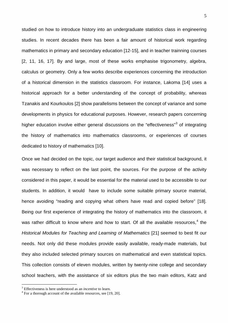
studied on how to introduce history into an undergraduate statistics class in engineering

studies. In recent decades there has been a fair amount of historical work regarding

mathematics in primary and secondary education [12-15], and in teacher trainning courses

[2, 11, 16, 17]. By and large, most of these works emphasise trigonometry, algebra,

calculus or geometry. Only a few works describe experiences concerning the introduction

of a historical dimension in the statistics classroom. For instance, Lakoma [14] uses a

historical approach for a better understanding of the concept of probability, whereas

Tzanakis and Kourkoulos [2] show parallelisms between the concept of variance and some

developments in physics for educational purposes. However, research papers concerning

higher education involve either general discussions on the “effectiveness”3

Once we had decided on the topic, our target audience and their statistical background, it

was necessary to reflect on the last point, the sources. For the purpose of the activity

considered in this paper, it would be essential for the material used to be accessible to our

students. In addition, it would have to include some suitable primary source material,

hence avoiding “reading and copying what others have read and copied before” [18].

Being our first experience of integrating the history of mathematics into the classroom, it

was rather difficult to know where and how to start. Of all the available resources,

of integrating

the history of mathematics into mathematics classrooms, or experiences of courses

dedicated to history of mathematics [10].

4

3 Effectiveness is here understood as an incentive to learn.

the

Historical Modules for Teaching and Learning of Mathematics [21] seemed to best fit our

needs. Not only did these modules provide easily available, ready-made materials, but

they also included selected primary sources on mathematical and even statistical topics.

This collection consists of eleven modules, written by twenty-nine college and secondary

school teachers, with the assistance of six editors plus the two main editors, Katz and

4 For a thorough account of the available resources, see [19, 20].

6

Michalowicz. In particular, there is a module on statistics covering basic concepts of

statistical reasoning, such as measures of central tendency, the normal distribution and

the method of least squares, as well as graphical representation of data.

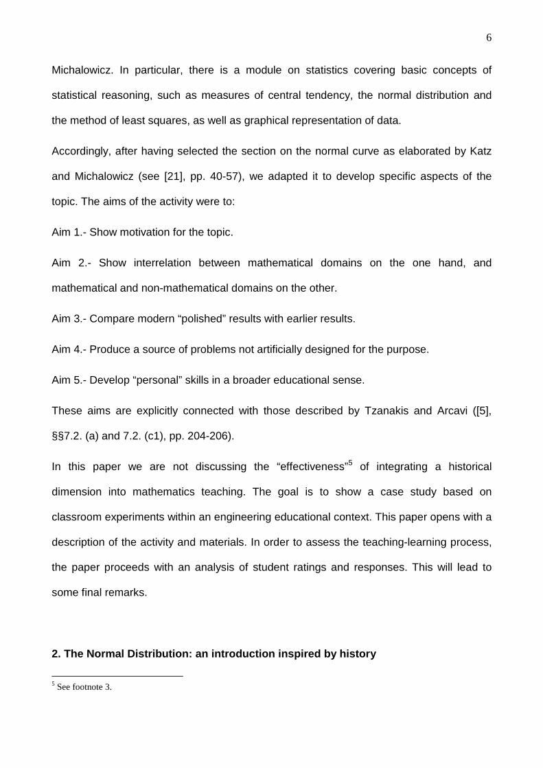
Accordingly, after having selected the section on the normal curve as elaborated by Katz

and Michalowicz (see [21], pp. 40-57), we adapted it to develop specific aspects of the

topic. The aims of the activity were to:

Aim 1.- Show motivation for the topic.

Aim 2.- Show interrelation between mathematical domains on the one hand, and

mathematical and non-mathematical domains on the other.

Aim 3.- Compare modern “polished” results with earlier results.

Aim 4.- Produce a source of problems not artificially designed for the purpose.

Aim 5.- Develop “personal” skills in a broader educational sense.

These aims are explicitly connected with those described by Tzanakis and Arcavi ([5],

§§7.2. (a) and 7.2. (c1), pp. 204-206).

In this paper we are not discussing the “effectiveness”5

of integrating a historical

dimension into mathematics teaching. The goal is to show a case study based on

classroom experiments within an engineering educational context. This paper opens with a

description of the activity and materials. In order to assess the teaching-learning process,

the paper proceeds with an analysis of student ratings and responses. This will lead to

some final remarks.

2. The Normal Distribution: an introduction inspired by history

5 See footnote 3.

7

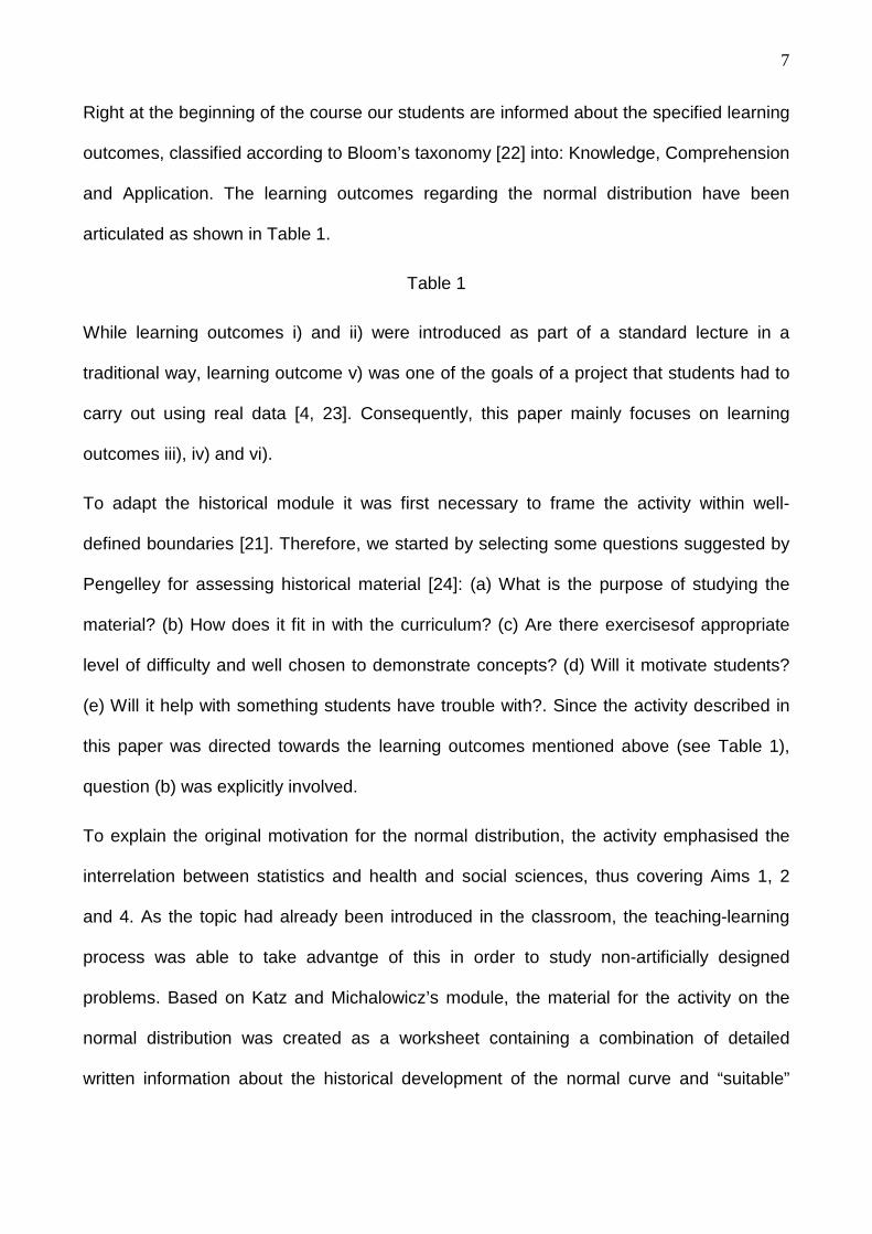
Right at the beginning of the course our students are informed about the specified learning

outcomes, classified according to Bloom’s taxonomy [22] into: Knowledge, Comprehension

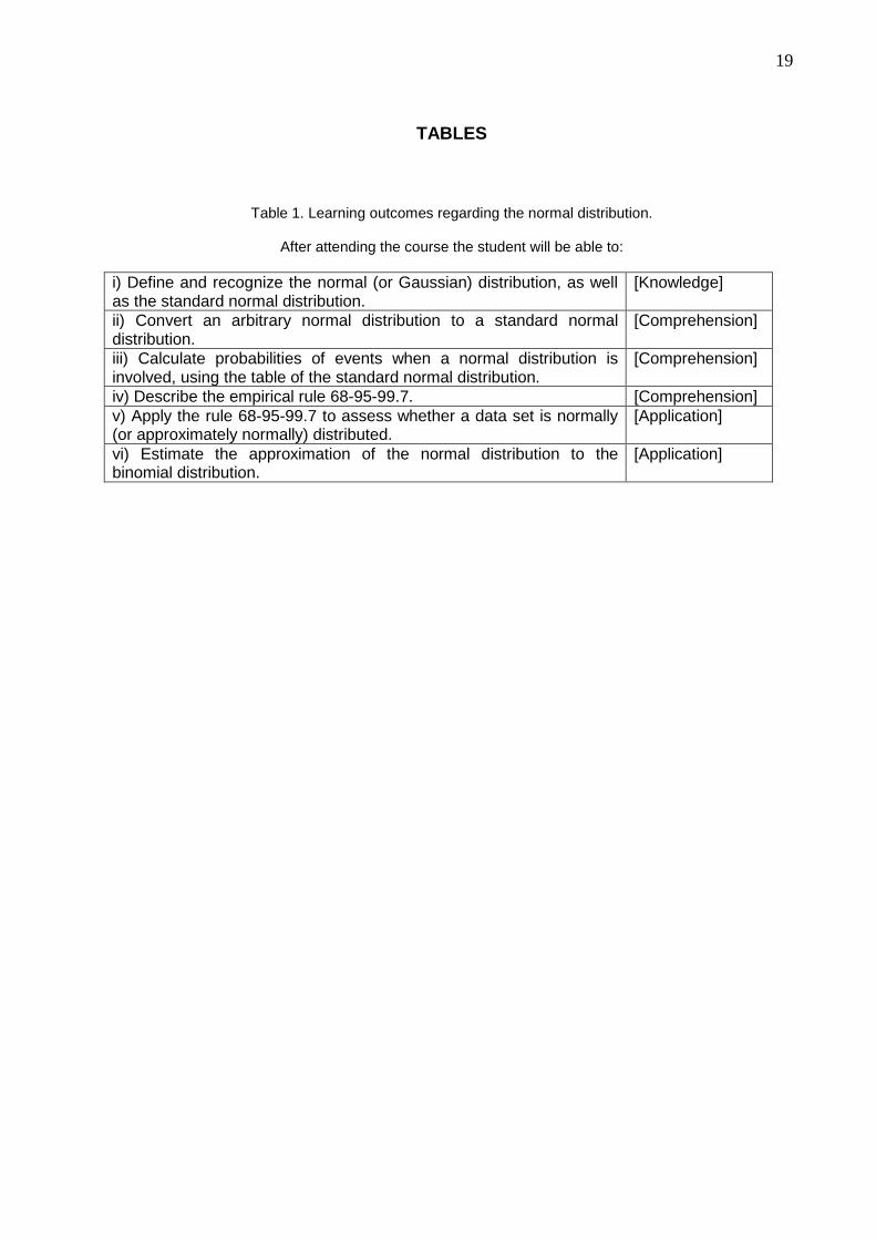
and Application. The learning outcomes regarding the normal distribution have been

articulated as shown in Table 1.

Table 1

While learning outcomes i) and ii) were introduced as part of a standard lecture in a

traditional way, learning outcome v) was one of the goals of a project that students had to

carry out using real data [4, 23]. Consequently, this paper mainly focuses on learning

outcomes iii), iv) and vi).

To adapt the historical module it was first necessary to frame the activity within well-

defined boundaries [21]. Therefore, we started by selecting some questions suggested by

Pengelley for assessing historical material [24]: (a) What is the purpose of studying the

material? (b) How does it fit in with the curriculum? (c) Are there exercisesof appropriate

level of difficulty and well chosen to demonstrate concepts? (d) Will it motivate students?

(e) Will it help with something students have trouble with?. Since the activity described in

this paper was directed towards the learning outcomes mentioned above (see Table 1),

question (b) was explicitly involved.

To explain the original motivation for the normal distribution, the activity emphasised the

interrelation between statistics and health and social sciences, thus covering Aims 1, 2

and 4. As the topic had already been introduced in the classroom, the teaching-learning

process was able to take advantge of this in order to study non-artificially designed

problems. Based on Katz and Michalowicz’s module, the material for the activity on the

normal distribution was created as a worksheet containing a combination of detailed

written information about the historical development of the normal curve and “suitable”

8

questions. There were no accompanying answer sheets as the task was designed to be

carried out in a two-hour computer lab session, individually or in pairs. Most of the

students worked individually, and only a few computers were shared by two students

working together. The teacher acted as a consultant during the session. The students

managed the time given over to each section of the activity themselves, according to their

individual needs and skills. If they were not able to finish their work in the computer lab,

they could do it as homework. It is worth pointing out that the questions were chosen not

only to assess understanding of the information provided, but also to bring out the

connection with other mathematical domains. Students were asked to prove expressions

and formulae, to use a spreadsheet to work out elementary probability calculations and to

represent data, and to investigate supplementary aspects regarding the contents of the

activity. All these aspects were planned in order to cover Aims 3 and 5.

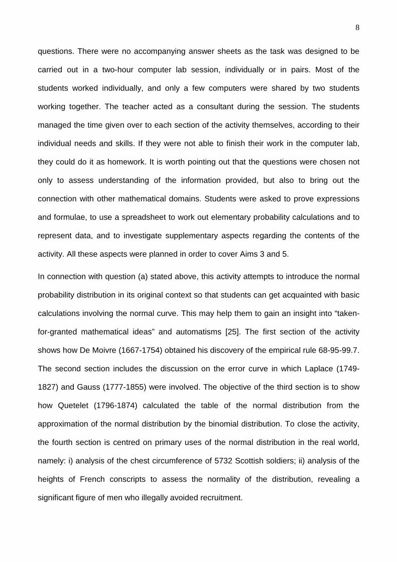
In connection with question (a) stated above, this activity attempts to introduce the normal

probability distribution in its original context so that students can get acquainted with basic

calculations involving the normal curve. This may help them to gain an insight into “taken-

for-granted mathematical ideas” and automatisms [25]. The first section of the activity

shows how De Moivre (1667-1754) obtained his discovery of the empirical rule 68-95-99.7.

The second section includes the discussion on the error curve in which Laplace (1749-

1827) and Gauss (1777-1855) were involved. The objective of the third section is to show

how Quetelet (1796-1874) calculated the table of the normal distribution from the

approximation of the normal distribution by the binomial distribution. To close the activity,

the fourth section is centred on primary uses of the normal distribution in the real world,

namely: i) analysis of the chest circumference of 5732 Scottish soldiers; ii) analysis of the

heights of French conscripts to assess the normality of the distribution, revealing a

significant figure of men who illegally avoided recruitment.

9

Given the limited time available for the session, the activity had to be carefully structured.

Unlike Katz and Michalowicz, we interspersed the text with seven leading questions,

conveniently placed after a specific topic or a related result, as opposed to a separate

sheet at the end. Questions 1, 4, 6 and 7 were directly inspired by the ones suggested by

Katz and Michalowicz (2005) on pages 46, 55, 56 and 57, respectively. The rest were

stated by us, to ensure that a particular point was fully understood. The questions were.

The following paragraphs briefly describe each question, drawing attention to the

educational aims served by each one.

Question 1: In an experiment in which 100 fair coins are flipped, about how many heads

would you expect to see? What is the corresponding standard deviation? Find the limits

(lower and upper) for the number of heads we would get 68%, 95% and 99.7% of the

times.

This first question deals with direct manipulation of a binomial distribution, followed by a

first encounter with the connection between the normal and the binomial distributions. It

was intended to help students “warm up” by stating a link between the activity and a topic

they had already learned in the classroom, thus relating to Aim 1.

Next, Questions 2, 3 and 4 are connected with Quetelet’s calculation of a symmetric

binomial distribution. His experiment was to draw 999 balls from an urn containing a large

number of balls, half of which were white, and half black.

Question 2: Prove Quetelet’s shortened procedure for the calculation of relative

probabilities: )(1

999)1( nXPn

nnXP =⋅+−

=+= , where )( nXP = represents the probability of

drawing n black balls from the urn. Setting the value of )500( =XP to be 1, calculate the

relative probabilities )501( =XP and )502( =XP .

10

Students had to deduce this recursive formula from the probability function of the binomial

distribution. This question was inserted to show the interrelation between mathematical

domains, namely, probability and recursive proofs (Aim 2). In this case the interest lies in

how to evaluate mathematical arguments and proofs, and to select and use appropriate

types of reasoning and methods of proof [8]. Given that students often meet difficulties in

proving recursive formulae, this exercise seems to be consistent with questions (c) and (e)

suggested above.

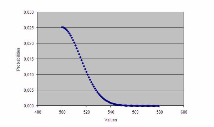
Question 3: Using an Excel worksheet recalculate column A of Quetelet’s table for the

values 500 to 579 and graph the corresponding curve.

To get a deeper knowledge of the binomial-normal link, students were asked at this point

to use a spreadsheet, in particular, the spreadsheet program Microsoft Excel (see Figure

1).. The computer practical classes offer students the possibility to be actively engaged in

the learning process, and to apply the concepts learned. As this topic is usually a source

of difficulty this exercise connects again with question (e). At the same time, it not only

helps to compare modern results with earlier ones, but also to develop “personal” skills

such as how to manipulate a spreadsheet. Therefore, this exercise focuses on Aims 3 and

5.

Figure 1

Question 4: A discrete variable can be approximated by a continuous variable considering

the following estimation:

continuousdiscrete kxkPkxP )5.05.0()( +≤≤−≈= .

For instance, normalbinomial xPxP )5.5005.499()500( ≤≤≈= .

Using this information, recalculate the first four values in column A using a modern table of

the normal distribution.

11

It can be assumed that the results of drawing balls out of the urn are normally distributed

with mean of the number of black balls equal to 500 and standard deviation equal to

8.1599921

≈ . Compare these results with Quetelet’s binomial table.

Understanding why we do things the way we do, and how mathematical concepts, terms

and symbols arose, plays a relevant role in grasping the topic (see [5], p. 5). Question 4

allowed the students to compare a modern table of the normal curve with the earliest table

through the use of the spreadsheet Excel. Thus Aim 3 is again involved in the proposed

activity. Although this question was taken from Katz and Michalowicz’s module, we

modified it by including some points regarding the link between discrete and continuous

variables.

Questions 5 and 6 concern some real world applications of the normal distribution.

Question 5: Read carefully Quetelet’s procedure for determining whether the chest

circumferences of the Scottish soldiers were normally distributed. Write down those points

you do not understand completely.

Question 6: From the results in the example of the heights of French conscripts, discuss

how Quetelet concluded there had been a fraud.

After reading and understanding the example on the chest circumferences (Question 5)

students were to draw conclusions in the case of the heights of French conscripts

(Question 6). However, as we will see in the following section, since Quetelet’s procedure

proved to be difficult to understand, less thant 20% of the students managed to answer

Question 6 correctly (“Good”).

Questions 4, 5 and 6 contribute to Aim 3 in that they help to compare historical results with

modern “polished” ones. Likewise, Aim 4 is also achieved since these questions convey

12

the idea that probabilistic tools represent a means of solving real-world problems, rather

than just artificially designed exercises, framed in a theoretical context.This set of

questions also encourages reading comprehension skills (Aim 5).

Finally, in Question 7 students were asked to search the Internet for information on “side

aspects” related to the normal distribution.

Question 7: Browse the Internet for information on Galton’s machine. What was the

relationship between the inventor Francis Galton (1822-1911) and Charles Darwin (1809-

1882)?

Originally suggested in Katz and Michalowicz’s module for further research, the intention

of this last question was to help develop some “personal” skills such as reading,

summarising, writing and documenting (Aim 5). At this point we found it interesting to point

out the interrelation between mathematical and non-mathematical domains, namely,

between statistics and the theory of evolution put forward by Darwin (Aim 2). A

fundamental part of Qestion 7 involves a writing component and documenting. The

incorporation of a writing component in statistics courses has been encouraged by Radke-

Sharpe [26] and Garfield [27]. Writing helps students to think about the assumptions

behind statistical, graphical or instrumental procedures, to formulate assumptions verbally,

and to examine the suitability of a particular procedure based on them. The inclusion of

documenting (i.e. browsing the Internet) facilitates student reading, understanding and

summarising from a range of sources. In short, reading, writing and documenting are tools

that will serve students well in their future scientific or academic writing. Encouraging

students to put concepts such as these into words will strengthen their understanding of

those concepts.

13

3. Assessment of the teaching-learning process

One of Pengelley’s questions mentioned above for assessing historical material (question

(d))[24] asks whether students will be motivated. Though not the only source of feedback,

student ratings provide an excellent guide for designing the teaching-learning process and

for assessing their motivation. Therefore, at the end of the activity students were asked to

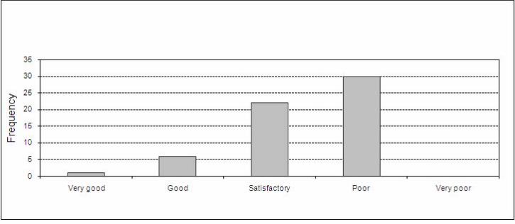
rate the activity thus:

(1) Very good, (2) Good, (3) Satisfactory, (4) Poor and (5) Very poor.

Figure 2 shows the results of this survey. Of the sixty students who took part in the

activity, half of them liked it (22 satisfactory, 6 good, 1 very good), whereas the other half

rated it as poor.

Figure 2

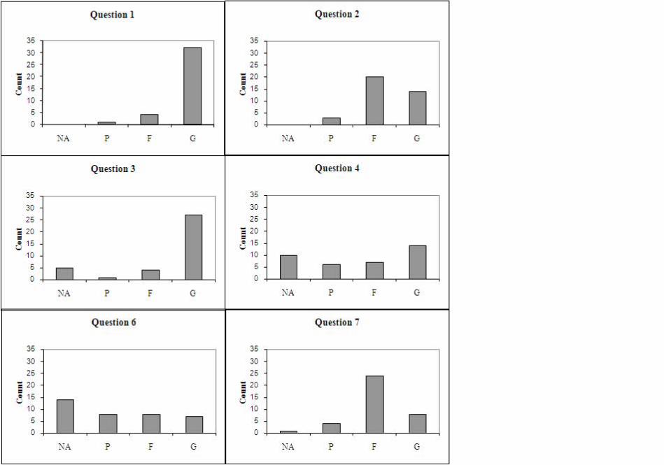
Another aspect suggested by Pengelley [24] for assessing historical material concerned

the degree of difficulty (question (c)). In order to determine this we analysed in detail the

sample of the thirty-seven students who had handed in their reports on the activity. Every

question (except Question 5) was marked with either Non-Answered, Poor, Fair or Good.

An analysis of the responses to the questions gives the following information. From the

graphics of Figure 3 regarding the assessment of the questions, it is clear that Questions 1

and 3 are most frequently marked as “Good” (86% and 68%, respectively). The fact that

Question 1 involved a routine use of a procedure previously worked in the classroom could

explain the extremely good results obtained in this question. As for Question 3, it is only

fair to mention that students were already acquainted with the facilities offered by the

spreadsheet Excel, not only the recursive computations, but also the graph options.

Question 2 obtained around 92% of the answers marked between “Fair” and “Good” (54%

and 38%, respectively). It turns out that those students with a “Fair” mark in this question

14

failed to prove the general recursive formula, just managing to check particular cases.

Question 4, although having the same ratio of answers marked “Good”, only obtained 19%

of “Fair” answers. The drawback here seems to be the link between the old and modern

procedures, probably because students were not sufficiently skilled in approximating a

discrete variable by a continuous one. Surprisingly, all the students answered questions 1

and 2, whereas the ratio of “Non-Answered” in Question 6 exceeds by far the rest of the

marked ratios (38%). As for Question 7, most of the students obtained “Fair”. This was

partly due to the fact that students merely copied information from the Internet and pasted

it on their worksheets, thus showing no interest in summarizing the information in their own

words.

Figure 3

As regards Question 5, from the comments given by our students we gathered that the

calculations involved in the construction of the table proved to be rather cumbersome and

time-consuming.

4. Final remarks

As Fauvel and van Maanen [9] point out, one should not underestimate the difficult task of

the teacher to achieve a proper transmission of historical knowledge into a productive

classroom activity for the learner. As this was our first experience using historical material

in the classroom, we were not able to foresee all the possible obstacles in the

understanding process. Now we are aware of certain difficulties inherent in the material

(for instance, in Questions 5 and 6). First of all, the mathematical language and form

(notation, computational methods, etc.) turned out to be rather confusing right from the

beginning. That is to say, students found it difficult to read source material in general, and

15

the unfamiliar language of the older primary sources in particular, as already pointed out

by Arcavi [11].

In addition, the syllabus and a sense of lack of time made us cram the activity into a two-

hour class. Likewise, we had some misgivings about how useful the topic was for our

students. Why not give them the opportunity to appreciate the topic itself, stressing the

aesthetics, intellectual curiosity, or the recreational purposes involved? Finally, we

borrowed and adapted part of Katz and Michalowicz’s historical modules on Statistics, but

for our particular syllabus, more didactic resource material on this topic would need to be

developed for future use.

On the whole, although it was challenging, the experience proved to be rewarding. Not

only did the activity supply a collection of non-artificially designed problems, but it also

helped to develop further skills, such as reading, writing and documenting. Above all, it

was a means to show the original motivation of the normal curve and thus, to make it more

understandable. This experience has shown that probability cannot be regarded as a

collection of “polished” products within a deductive structured system, but rather as a

system with a peculiar life (expectations, false expectations and false starts), as de

Guzmán [28] put it, determined and influenced by external factors and connected with

mathematical and non-mathematical domains. Hence, insofar as the activity fostered

cross-curricular competences, it was certainly designed in keeping with the guidelines of

the EHEA.

Acknowledgements

We are especially indebted to V. Katz and M. K. Michalowicz for having been able to use

their historical modules. We wish to thank C. Tzanakis for comments on an earlier draft of

this paper and M. Skidmore for revising our English.

16

References

[1] M. Blanco and M. Ginovart, Introducing the normal distribution by following a teaching

approach inspired by history: an example for classroom implementation in engineering

education, Proceedings of the Sixth Conference European Research in Mathematics

Education, 2009 (in press).

[2] C. Tzanakis and M. Kourkoulos, May history and physics provide a useful aid for

introducing basic statistical concepts?, Proceedings of the HPM satellite meeting of ICME-

10 & the 4th Summer University on the history and epistemology in mathematics

education, Uppsala, 2004.

[3] M. Meletiou, On the formalist view of mathematics: impact on statistics instruction and

learning, Proceedings of the Third European Conference in Mathematics Education,

Bellaria, 2003.

[4] M. Blanco and M. Ginovart, La probabilidad y la utilización de la plataforma virtual

Moodle en las enseñanzas técnicas dentro del marco del Espacio Europeo de Educación

Superior, Proceedings of the XVI Congreso Universitario de Innovación Educativa en las

Enseñanzas Técnicas, Cádiz, 2008.

[5] C. Tzanakis and A. Arcavi, Integrating history of mathematics in the classroom: an

analytic survey, in History in mathematics education: the ICMI study, J. Fauvel and J. van

Maanen, eds., Kluwer, Dordrecht, 2000, pp. 201-240.

[6] F. J. Swetz, J. Fauvel, O. Bekken, B. Johansson and V. Katz, eds., Learn from the

Masters, The Mathematical Association of America, Washington, 1995.

[7] J. Fauvel, Using history in mathematics education, Learn. Math. 11 (1991), pp. 3-6.

[8] R. Ellington, The importance of incorporating the history of mathematics into the

Standards 2000 draft and the overall mathematics curriculum, EDCI 650 Reacts: History of

17

Mathematics, University of Maryland, 1998. Available at

http://www.math.umd.edu/~dac/650old/ellingtonpaper.html (accessed 14 January 2009).

[9] J. Fauvel and J. van Maanen, eds., History in mathematics education: the ICMI study,

Kluwer, Dordrecht, 2000.

[10] D. Fowler, Perils and pitfalls of history, Learn. Math. 11 (1991), pp. 15-16.

[11] A. Arcavi, M. Bruckheimer and R. Ben-Zvi, Maybe a mathematics teacher can profit

from the study of the history of mathematics, Learn. Math. 3 (1982), pp. 30-37.

[12] J. H. Gardner, “How fast does the wind travel?”: history in the primary mathematics

classroom, Learn. Math. 11 (1991), pp. 17-20.

[13] J. van Maanen, L’Hôpital’s weight problem, Learn. Math. 11 (1991), pp. 44-47.

[14] E. Lakoma, How may history help the teaching of probabilistic concepts?, in History in

mathematics education: the ICMI study, J. Fauvel and J. van Maanen, eds., Kluwer,

Dordrecht, 2000, pp. 248-252.

[15] M. R. Massa, F. Romero and I. Guevara, Teaching mathematics through history:

some trigonometric concepts, Proceedings of the Second International Conference of the

European Society for the History of Science, Cracow, 2006.

[16] G. Schubring, History of mathematics for trainee teachers, in Integrating history of

mathematics in the classroom: an analytic survey, in History in mathematics education: the

ICMI study, J. Fauvel and J. van Maanen, eds., Kluwer, Dordrecht, 2000, pp. 91-142.

[17] E. Barbin, The reading of original texts: how and why to introduce a historical

perspective, Learn. Math. 11 (1991), pp. 12-13.

[18] H. Freudenthal, Should a mathematics teacher know something about the history of

mathematics?, Learn. Math. 2 (1981), pp. 30-33.

[19] J. Barrow-Green, History of mathematics: resources on the world wide web, Math.

Sch. 27 (1998), pp. 16-22.

18

[20] L. Rogers, History of mathematics: resources for teachers, Learn. Math. 11 (1991),

pp. 48-51.

[21] V. J. Katz and K. D. Michalowicz, eds., Historical Modules for the Teaching and

Learning of Mathematics, The Mathematical Association of America, Washington, 2005.

[22] B. S. Bloom, ed., Taxonomy of Education Objectives: Handbook I: Cognitive Domain,

David McKay Company, New York, 1956. Available at

http://faculty.washington.edu/krumme/guides/bloom1.html (accessed 14 January 2009).

[23] M. Blanco and M. Ginovart, Suggestions for Teaching Exploratory Data Analysis in

Engineering Education within the European Credit Transfer System, Proceedings of the

CIEAEM 59 - Mathematical activity in classroom practice and as research object in

didactics: two complementary perspectives, Dobogókö, 2007.

[24] D. J. Pengelley, A graduate course on the role of history in teaching mathematics. In

Study the Masters: the Abel-Fauvel Conference, O. Becken, ed., National Center for

Mathematics Education, University of Gothenburg, Gothenburg, 2002. Available at

http://www.math.nmsu.edu/~davidp/gradcourserolehist.pdf (accessed 14 January 2009).

[25] A. Arcavi, Two benefits of using history, Learn. Math. 11 (1991), p. 11.

[26] N. Radke-Sharpe, Writing As a Component of Statistics Education, Amer. Statist. 45

(1991), pp. 292-293.

[27] J. Garfield, Beyond Testing and Grading: Using Assessment to Improve Student

Learning, J. Stat. Educ. 2 (1994). Available at

http://www.amstat.org/publications/jse/v2n1/garfield.html (accessed 14 January 2009).

[28] M. de Guzmán, Origin and Evolution of Mathematical Theories: Implications for

Mathematical Education, HPM Newsletter 8 (1993), pp. 2-3.

19

TABLES

Table 1. Learning outcomes regarding the normal distribution.

After attending the course the student will be able to:

i) Define and recognize the normal (or Gaussian) distribution, as well as the standard normal distribution.

[Knowledge]

ii) Convert an arbitrary normal distribution to a standard normal distribution.

[Comprehension]

iii) Calculate probabilities of events when a normal distribution is involved, using the table of the standard normal distribution.

[Comprehension]

iv) Describe the empirical rule 68-95-99.7. [Comprehension] v) Apply the rule 68-95-99.7 to assess whether a data set is normally (or approximately normally) distributed.

[Application]

vi) Estimate the approximation of the normal distribution to the binomial distribution.

[Application]

20

FIGURES

Figure 1. Graph corresponding to Question 3 in a student’s report.

Figure 2. Student ratings on the activity.

Figure 3. Assessment of the questions in the activity with Non-Answered (NA), Poor (P), Fair (F) or Good

(G).