How to increase the odds of owning the few stocks that ... · portfolio’s number of randomly selected stocks, investors are more likely to include those stocks with higher magnitudes

Vanguard Research February 2019

How to increase the odds of owning the few stocks that drive returns

■ Some investment strategists advocate concentrated, “best ideas” portfolios as the surest path to equity market outperformance. The premise is obvious: when a portfolio consists only of a manager’s best ideas, returns are undiluted by second-best or lesser ideas. But the reality is different.

■ We use simulations and empirical analysis to evaluate the relationship between portfolio diversification and outperformance. Rather than raise the outperformance odds, increasing concentration lowers them. The less diversified a portfolio, the less likely it is to hold the small percentage of stocks that account for most of the market’s long-term return. Concentration can increase the odds of earning high margins of outperformance, but the probability of missing that return target increases more quickly than the probability of reaching it.

■ Our analysis yields two measures that a manager must meet to outperform the market: the “excess return hurdle” and the “success rate”. The excess return hurdle is the expected gap between portfolio and market returns at different levels of concentration, and our analysis shows this decreases with increased holdings. Success rate is a measure of the manager’s ability to identify outperformers. The success rate necessary for a portfolio to outperform decreases as the number of holdings increases.

Chris Tidmore, CFA; Francis M. Kinniry Jr., CFA; Giulio Renzi-Ricci; Edoardo Cilla

Acknowledgement: The authors would like to thank Andrew S. Clarke, CFA, Daniel B. Berkowitz, CFA, and Lucas Baynes for their contributions to this research.

For professional investors only as defined under the MiFID II Directive. Not for public distribution. In Switzerland for professional investors only. Not to be distributed to the public.

This document is published by The Vanguard Group, Inc. It is for educational purposes only and is not a recommendation or solicitation to buy or sell investments. It should be noted that it is written in the context of the US market and contains data and analysis specific to the US.

2

Notes on risk

All investing is subject to risk, including possible loss of principal. Past performance is no guarantee of future returns. Diversification does not ensure a profit or protect against a loss. The performance of an index is not an exact representation of any particular investment, as you cannot invest directly in an index.

Many investors and financial professionals believe that broadly diversified portfolios are inferior to concentrated portfolios made up of a manager’s “best ideas”. This belief has been informed by research showing that portfolio managers’ “top picks” have tended to outperform the rest of their holdings (Cohen, Polk, and Silli, 2010, and Yeung et al., 2012). The premise seems straightforward: when assets are concentrated in a manager’s best ideas, the performance of these securities is undiluted by less promising ideas. Despite the intuitive appeal of this premise, theoretical and empirical research fails to validate it. Why?

We address this question in three steps. First, we explore the concept that a portfolio’s best ideas can be extracted from a more diversified portfolio to create a more concentrated one that will produce returns equal to those of the “best ideas” subset. This assumption reflects hindsight bias that obscures the difficulty of identifying a portfolio’s best ideas.

Second, we conduct simulations to build randomly selected, equal-weighted portfolios with varying numbers of holdings. We find that the more broadly diversified portfolios (those with relatively more holdings) outperform the more concentrated ones (those with relatively fewer holdings but also a tighter dispersion of excess returns). Consistent with work by Ikenberry, Shockley, and Womack (1998); Heaton, Polson, and Witte (2017); and Bessembinder (2018), our analysis highlights the risk of excluding the minority of stocks that produce an outsized share of the market’s return in any given period. It also yields parameters such as the “excess return hurdle” or the stock-selection “success rate” a manager must clear to outperform at different levels of portfolio concentration.

Finally, we complement the simulated analysis with an empirical analysis of the historical performance of US mutual funds. The empirical analysis uses panel data regression to estimate to what extent mutual fund

excess returns are explained by the number of holdings. The empirical results are consistent with our theoretical analysis, though they are notably time-period-dependent.

Discerning what an active manager’s best ideas were is not easy

A simple review of an active manager’s portfolio can yield misleading conclusions about the manager’s best ideas. For example, it seems reasonable to assume that the largest positions are the best ideas – those in which the manager has the greatest conviction. A simple illustration, though, shows why this assumption can be misplaced. It argues against the conclusions drawn in research such as Yeung et al. (2012) that derived concentrated results from diversified fund portfolios.

Consider an active manager that begins with five great ideas and allocates assets evenly to all five. At the end of the fund’s first year, Stock A has appreciated 30%, Stock B 20%, and Stock C 10%, while Stock D has returned 0% and Stock E –10%. As shown in Figure 1, Stock A is now the largest holding and was the best performer for the year, but it wasn’t the best idea; it was one of five equally good ideas.

The initial best ideas may also not start out intended as such. A manager may be adept at adding to the more profitable positions over time. In this case, the “best idea” is not a permanent designation, but rather a dynamic status contingent on performance, new information, and/or insight. Other managers may be good at cutting back or eliminating their losing positions. Some best ideas may entail significant risk, and so the manager may proactively keep the position small. In each of these cases, it would be inaccurate to conclude that the current largest positions were the initial or current best ideas and should have been the sole investments in the manager’s portfolio.


3

1 In addition, long-horizon returns of stocks exhibit positive skew both because monthly returns are positively skewed and because the compounding of random returns creates positive skew in a multiperiod distribution. For further details and a more in-depth discussion underlying a similar analysis and results, see Bessembinder (2018)

For professional investors only as defined under the MiFID II Directive. Not for public distribution. In Switzerland for professional investors only. Not to be distributed to the public..

Concentration, risk, and return: A bottom-up analysis

Assessing the benefits of diversification within equities is important, and significant research has been done on how many stocks constitute proper diversification. Graham (1949), Evans and Archer (1968), Fisher and Lorie (1970), Malkiel (1973), and Statman (2004) mostly addressed the effect of a portfolio’s size on its nonsystematic risk but not on its return. Because the return distribution of stocks exhibits positive skew, we look to further address the question of concentration from both risk and return perspectives using historical stock performance.

Historical individual stock returns

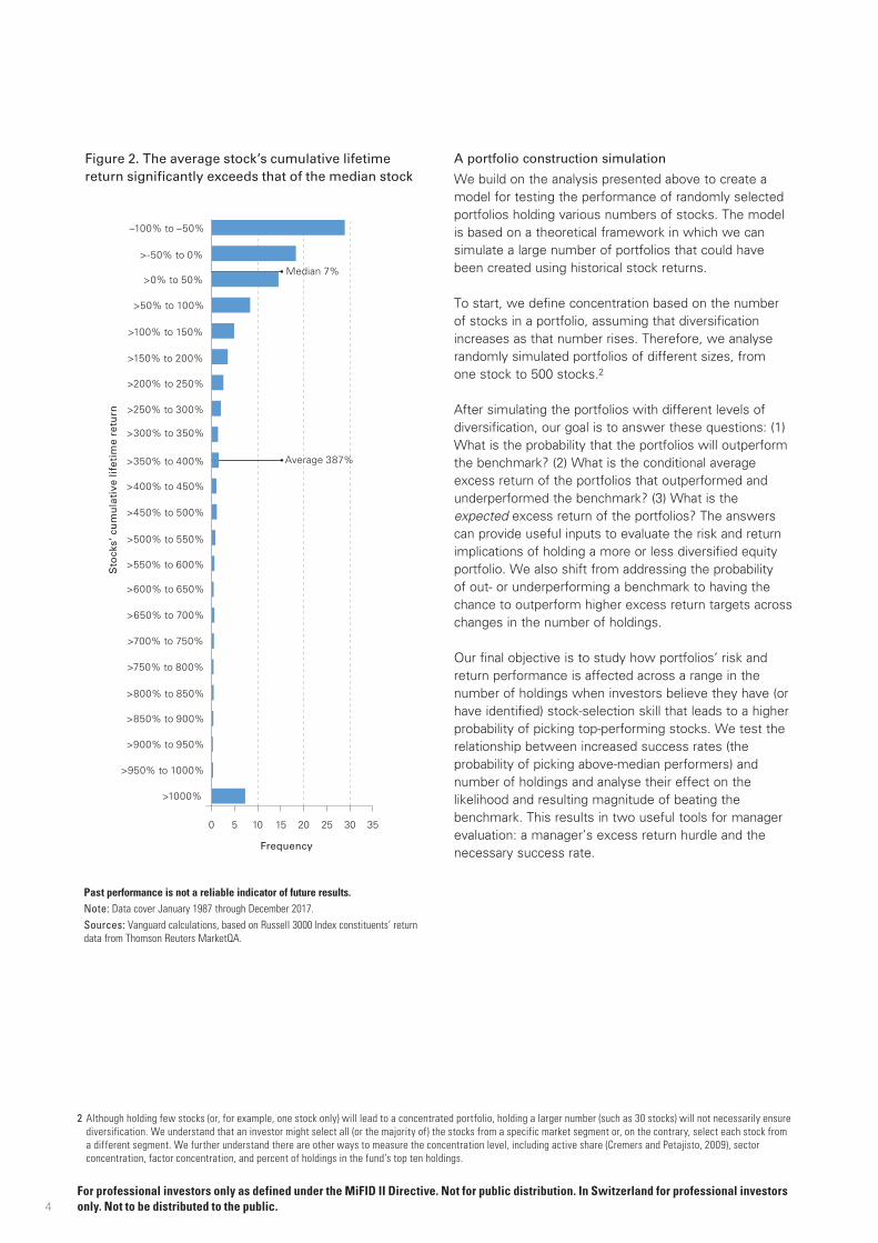
We confirm the work by Ikenberry, Shockley, and Womack (1998); Heaton, Polson, and Witte (2017); and Bessembinder (2018), among others, which showed that, because of the skewness of cumulative equity returns, a minority of stocks are responsible for the market’s cumulative gains. The majority of stocks throughout history have been relative losers. We conducted a similar analysis by calculating the cumulative returns of stocks in the Russell 3000 Index for January 1987 through December 2017, and the results were consistent. Figure 2, on page 4, displays the frequency of cumulative returns as well as the median and average values, and it shows, like Cembalest (2014) and Edwards and Lazzara (2016), that approximately 47% of stocks were unprofitable investments and that almost 30% lost more than half their value. On the other hand, roughly 7% of stocks had cumulative returns over 1,000%.

Figure 2 shows that the median stock’s lifetime return was 7%, whereas the average stock in a portfolio composed of all available stocks returned 387%. In fact, as we start from one stock and add more stocks to the portfolio, the portfolio return is more likely to improve from the median to the average stock return. This is because the probability of owning the market’s extreme winners increases. This implies that by increasing a portfolio’s number of randomly selected stocks, investors are more likely to include those stocks with higher magnitudes of return. This is key, because the high-magnitude returns of a smaller number of stocks outweighs the lower – or even negative – returns of a larger number of stocks.1

Figure 1. Larger positions may be due more to market performance than to initial best ideas

Any projections should be regarded as hypothetical in nature and do not reflect or guarantee future results.Source: Vanguard.

0.00

0.05

0.10

0.15

0.20

0.25

Initial allocationEnd of year

Po

rtfo

lio w

eig

hti

ng

Stock A Stock B Stock C Stock D Stock E

4

2 Although holding few stocks (or, for example, one stock only) will lead to a concentrated portfolio, holding a larger number (such as 30 stocks) will not necessarily ensure diversification. We understand that an investor might select all (or the majority of) the stocks from a specific market segment or, on the contrary, select each stock from a different segment. We further understand there are other ways to measure the concentration level, including active share (Cremers and Petajisto, 2009), sector concentration, factor concentration, and percent of holdings in the fund’s top ten holdings.


A portfolio construction simulation

We build on the analysis presented above to create a model for testing the performance of randomly selected portfolios holding various numbers of stocks. The model is based on a theoretical framework in which we can simulate a large number of portfolios that could have been created using historical stock returns.

To start, we define concentration based on the number of stocks in a portfolio, assuming that diversification increases as that number rises. Therefore, we analyse randomly simulated portfolios of different sizes, from one stock to 500 stocks.2

After simulating the portfolios with different levels of diversification, our goal is to answer these questions: (1) What is the probability that the portfolios will outperform the benchmark? (2) What is the conditional average excess return of the portfolios that outperformed and underperformed the benchmark? (3) What is the expected excess return of the portfolios? The answers can provide useful inputs to evaluate the risk and return implications of holding a more or less diversified equity portfolio. We also shift from addressing the probability of out- or underperforming a benchmark to having the chance to outperform higher excess return targets across changes in the number of holdings.

Our final objective is to study how portfolios’ risk and return performance is affected across a range in the number of holdings when investors believe they have (or have identified) stock-selection skill that leads to a higher probability of picking top-performing stocks. We test the relationship between increased success rates (the probability of picking above-median performers) and number of holdings and analyse their effect on the likelihood and resulting magnitude of beating the benchmark. This results in two useful tools for manager evaluation: a manager’s excess return hurdle and the necessary success rate.

Figure 2. The average stock’s cumulative lifetime return significantly exceeds that of the median stock

Past performance is not a reliable indicator of future results.Note: Data cover January 1987 through December 2017.Sources: Vanguard calculations, based on Russell 3000 Index constituents’ return data from Thomson Reuters MarketQA.

Frequency

>1000%

>950% to 1000%

>900% to 950%

>850% to 900%

>800% to 850%

>750% to 800%

>700% to 750%

>650% to 700%

>600% to 650%

>550% to 600%

>500% to 550%

>450% to 500%

>400% to 450%

>350% to 400%

>300% to 350%

>250% to 300%

>200% to 250%

>150% to 200%

>100% to 150%

>50% to 100%

>0% to 50%

>-50% to 0%

–100% to –50%

0 5 10 15 20 25 30 35

Median 7%

Average 387%

Sto

cks’

cu

mu

lati

ve li

feti

me

retu

rn

5

3 We understand that using the stocks in a segment of the Russell 3000 Index, such as the Russell 1000 Index or Russell 2000 Index, could lead to different results.4 We also tested annual rebalancing with similar results.5 We define tracking error as the annualised standard deviation of excess returns.6 We believe that using the stocks included in the Russell 3000 Index universe can help avoid the problem of picking microcapitalisation stocks that cannot be easily

traded.7 We believe this assumption is reasonable, as reallocating the capital to the remaining stocks could increase the portfolio’s concentration during the rebalancing period.


Data and methodology

Our dataset encompasses the universe of stocks of the Russell 3000 Index from January 1987 through December 2017.3 For each stock, we use monthly returns. Our analysis also assumes that a hypothetical investor would invest her or his capital over the entire data sample period.

We create time series of portfolio performance as follows:

1. At the beginning of each quarterly rebalancing period, we randomly select stocks to form portfolios holding n stocks where n equals 1, 5, 10, 15, 30, 50, 100, 200, or 500.4 Each stock must exist at the beginning of the quarter and has an equal probability of selection. Each portfolio is created independently (so the same stock could appear in more than one portfolio).

2. After selecting the stocks, we construct the portfolio by equally weighting them.

3. We then compare each portfolio’s performance with that of the equal-weighted benchmark and check whether the portfolio outperformed or underperformed the benchmark. For each portfolio, we also compute the excess return and tracking error versus the benchmark.5

4. For each portfolio size, we conduct the above three steps 10,000 times, and we compute average risk and return summary statistics.

To analyse the risk and return profile of the simulated portfolios, we make three assumptions:

• We have equally weighted the stocks in every portfolio and have defined the benchmark as the equal-weighted market portfolio made up of all stocks available at each point in time in the Russell 3000 Index.6 For the purpose of this analysis, and thus to isolate the effect of concentration, it is important to use the same weighting method for both portfolio and benchmark, to reduce potential bias resulting from stock characteristics (for example, small-capitalisation bias).

• Should one or more stocks that have been selected be removed from the benchmark during the investment period, we assume that the corresponding capital is invested in cash paying no interest.7

• Because our goal is to build a theoretical framework to compare levels of concentration in portfolios, our analysis does not consider management fees and transaction costs. Depending on their magnitude, including this information could lead to different results.

Simulation results

We ran 10,000 simulations for each portfolio size to first calculate the percentage of the portfolios that would outperform the benchmark.

6

8 We have also tested portfolios with a higher number of holdings, up to the extreme case of n–1 stocks, where n is the number of stocks in the benchmark at any point in time. In this case, the probability of outperforming the benchmark converges to 50%; this is justified by the fact that we defined the benchmark as the arithmetic average of all stocks in the universe.

9 When we ran the simulations over longer periods, the probability of outperformance decreased across all numbers of stock holdings, and the fewer the holdings, the greater the magnitude of decline.

10 We also analysed median performance with quantitatively similar results.


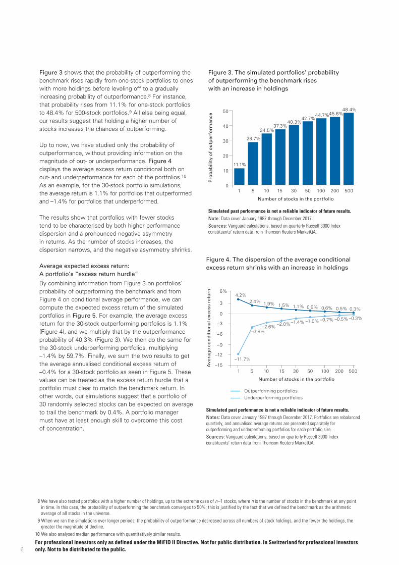
Figure 3 shows that the probability of outperforming the benchmark rises rapidly from one-stock portfolios to ones with more holdings before leveling off to a gradually increasing probability of outperformance.8 For instance, that probability rises from 11.1% for one-stock portfolios to 48.4% for 500-stock portfolios.9 All else being equal, our results suggest that holding a higher number of stocks increases the chances of outperforming.

Up to now, we have studied only the probability of outperformance, without providing information on the magnitude of out- or underperformance. Figure 4 displays the average excess return conditional both on out- and underperformance for each of the portfolios.10 As an example, for the 30-stock portfolio simulations, the average return is 1.1% for portfolios that outperformed and –1.4% for portfolios that underperformed.

The results show that portfolios with fewer stocks tend to be characterised by both higher performance dispersion and a pronounced negative asymmetry in returns. As the number of stocks increases, the dispersion narrows, and the negative asymmetry shrinks.

Average expected excess return: A portfolio’s “excess return hurdle”

By combining information from Figure 3 on portfolios’ probability of outperforming the benchmark and from Figure 4 on conditional average performance, we can compute the expected excess return of the simulated portfolios in Figure 5. For example, the average excess return for the 30-stock outperforming portfolios is 1.1% (Figure 4), and we multiply that by the outperformance probability of 40.3% (Figure 3). We then do the same for the 30-stock underperforming portfolios, multiplying –1.4% by 59.7%. Finally, we sum the two results to get the average annualised conditional excess return of –0.4% for a 30-stock portfolio as seen in Figure 5. These values can be treated as the excess return hurdle that a portfolio must clear to match the benchmark return. In other words, our simulations suggest that a portfolio of 30 randomly selected stocks can be expected on average to trail the benchmark by 0.4%. A portfolio manager must have at least enough skill to overcome this cost of concentration.

Figure 3. The simulated portfolios’ probability of outperforming the benchmark rises with an increase in holdings

Simulated past performance is not a reliable indicator of future results.Note: Data cover January 1987 through December 2017.Sources: Vanguard calculations, based on quarterly Russell 3000 Index constituents’ return data from Thomson Reuters MarketQA.

0

10

20

30

40

50

Pro

bab

ility

of

ou

tper

form

ance

1

11.1%

5

28.7%

10

34.5%

15

37.3%

30

40.3%

50

42.7%

100

44.7%

200

45.6%

500

48.4%

Number of stocks in the portfolio

Figure 4. The dispersion of the average conditional excess return shrinks with an increase in holdings

Simulated past performance is not a reliable indicator of future results.Notes: Data cover January 1987 through December 2017. Portfolios are rebalanced quarterly, and annualised average returns are presented separately for outperforming and underperforming portfolios for each portfolio size.Sources: Vanguard calculations, based on quarterly Russell 3000 Index constituents’ return data from Thomson Reuters MarketQA.

Notes: dot size = p4

to change size: select same appearance; go to effect > convert to shape > ellipse > absolute

0%

20%

40%

60%

80%

100%

-6 -4 -2 0 2 4 6

-15

-10

-5

0

5

10

15

0%

100%

200%

300%

400%

500%

2012201120102009200820072006200520042003

1p

5th

95th

Percentileskey:

75th

25th

Median

5th

95th

Percentileskey:

75th

25th

Median

–6

–3

0

3

6

9

12

15%

Top Bottom

Axi

s la

bel

if n

eed

ed

Axis label if needed

-6%

-3%

0%

3%

6%

9%

12%

15%

0.0

0.1

0.2

0.3

0.4

0.5

0.6

0.7

0.8

0.0

0.1

0.2

0.3

0.4

0.5

0.6

0.7

0.8

Outperforming portfoliosUnderperforming portfolios

Ave

rag

e co

nd

itio

nal

exc

ess

retu

rn


–15

–6

–9

–12

–3

3

0

6%

1 5 10 15 30 50 100 200 5000

10

20

30

40

50

60

70

80%

Axi

s la

bel

if n

eed

ed

4.2%2.4% 1.9% 1.5% 1.1% 0.9% 0.6% 0.5% 0.3%

–11.7%

–3.8%–2.6% –2.0%–1.4% –1.0% –0.7% –0.5% –0.3%

7

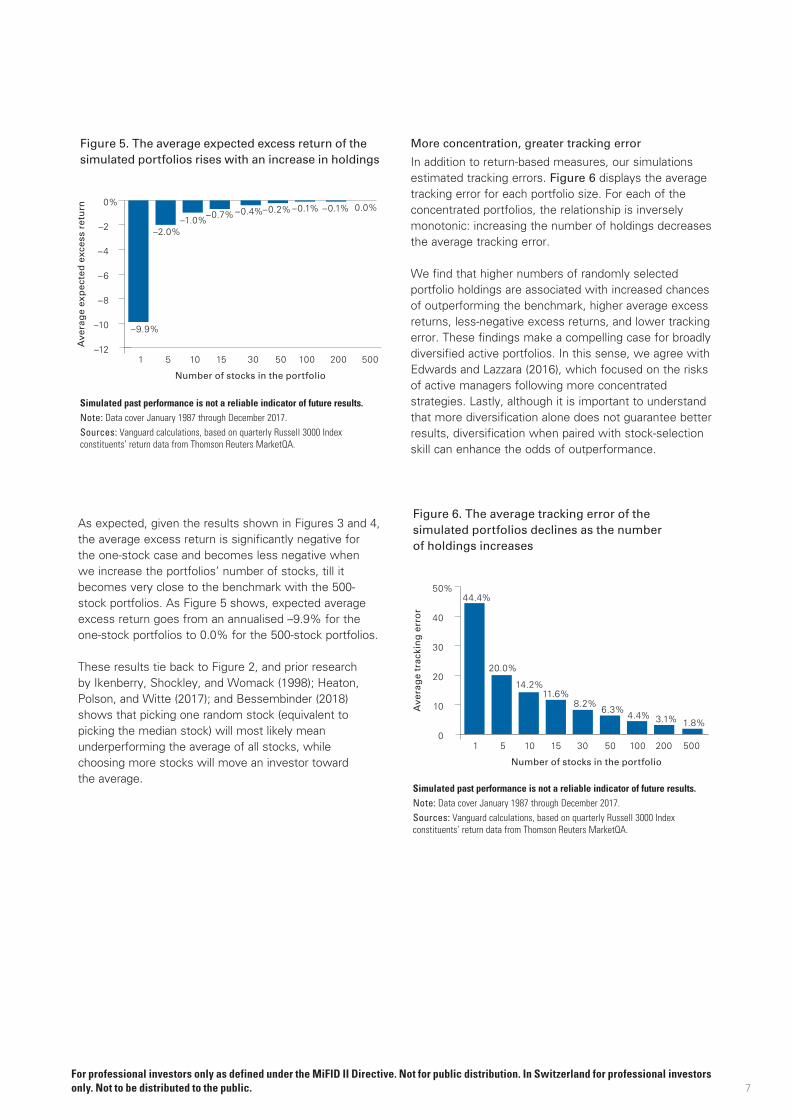
As expected, given the results shown in Figures 3 and 4, the average excess return is significantly negative for the one-stock case and becomes less negative when we increase the portfolios’ number of stocks, till it becomes very close to the benchmark with the 500-stock portfolios. As Figure 5 shows, expected average excess return goes from an annualised –9.9% for the one-stock portfolios to 0.0% for the 500-stock portfolios.

These results tie back to Figure 2, and prior research by Ikenberry, Shockley, and Womack (1998); Heaton, Polson, and Witte (2017); and Bessembinder (2018) shows that picking one random stock (equivalent to picking the median stock) will most likely mean underperforming the average of all stocks, while choosing more stocks will move an investor toward the average.

More concentration, greater tracking error

In addition to return-based measures, our simulations estimated tracking errors. Figure 6 displays the average tracking error for each portfolio size. For each of the concentrated portfolios, the relationship is inversely monotonic: increasing the number of holdings decreases the average tracking error.

We find that higher numbers of randomly selected portfolio holdings are associated with increased chances of outperforming the benchmark, higher average excess returns, less-negative excess returns, and lower tracking error. These findings make a compelling case for broadly diversified active portfolios. In this sense, we agree with Edwards and Lazzara (2016), which focused on the risks of active managers following more concentrated strategies. Lastly, although it is important to understand that more diversification alone does not guarantee better results, diversification when paired with stock-selection skill can enhance the odds of outperformance.

Figure 5. The average expected excess return of the simulated portfolios rises with an increase in holdings


–12

–10

–8

–6

–4

–2

0%

Ave

rag

e ex

pec

ted

exc

ess

retu

rn

1

–9.9%

5

–2.0%

10

–1.0%

15

–0.7%

30

–0.4%

50

–0.2%

100

–0.1%

200

–0.1%

500

0.0%


Figure 6. The average tracking error of the simulated portfolios declines as the number of holdings increases


0

10

20

30

40

50%

Ave

rag

e tr

acki

ng

err

or

1

44.4%

5

20.0%

10

14.2%

15

11.6%

30

8.2%

50

6.3%

100

4.4%

200

3.1%

500

1.8%0

10

20

30

40

50

60

70

80%

Axi

s la

bel

if n

eed

ed



8

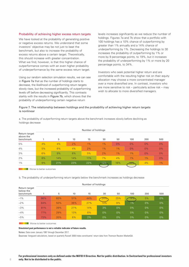
Figure 7. The relationship between holdings and the probability of achieving higher return targets is nonlinear

a. The probability of outperforming return targets above the benchmark increases slowly before declining as holdings decrease

Number of holdings

Return target above the benchmark 1 5 10 15 30 50 100 200 500

5% 4% 4% 2% 1% 1% 0% 0% 0% 0%

4% 5% 6% 4% 2% 1% 1% 0% 0% 0%

3% 6% 9% 8% 5% 2% 1% 1% 0% 0%

2% 8% 14% 14% 11% 7% 4% 1% 1% 0%

1% 9% 21% 23% 22% 19% 16% 10% 4% 1%

b. The probability of underperforming return targets below the benchmark increases as holdings decrease

Number of holdings

Return target below the benchmark 1 5 10 15 30 50 100 200 500

–1% 86% 60% 51% 44% 34% 25% 14% 5% 0%

–2% 84% 50% 36% 27% 14% 6% 1% 0% 0%

–3% 81% 39% 27% 14% 3% 0% 0% 0% 0%

–4% 77% 29% 13% 6% 0% 0% 0% 0% 0%

–5% 73% 20% 6% 2% 0% 0% 0% 0% 0%

Simulated past performance is not a reliable indicator of future results.

Notes: Data cover January 1987 through December 2017.Sources: Vanguard calculations, based on quarterly Russell 3000 Index constituents’ return data from Thomson Reuters MarketQA.

Probability of achieving higher excess return targets

We have looked at the probability of generating positive or negative excess returns. We understand that some investors’ objective may be not just to beat the benchmark, but also to increase the probability of excess returns above a certain target. Theoretically, this should increase with greater concentration. What we find, however, is that this higher chance of outperformance comes with an even higher probability of underperformance by the same excess return target.

Using our random selection simulation results, we can see in Figure 7a that as the number of holdings starts to decrease, the likelihood of outperforming return targets slowly rises, but the increased probability of outperforming levels off before decreasing significantly. This contrasts starkly with the results in Figure 7b, which shows that the probability of underperforming certain negative return

levels increases significantly as we reduce the number of holdings. Figures 7a and 7b show that a portfolio with 100 holdings has a 10% chance of outperforming by greater than 1% annually and a 14% chance of underperforming by 1%. Decreasing the holdings to 30 increases the probability of outperforming by 1% or more by 9 percentage points, to 19%, but it increases the probability of underperforming by 1% or more by 20 percentage points, to 34%.

Investors who seek potential higher return and are comfortable with the resulting higher risk on their equity allocation may choose a more concentrated manager over a more diversified one. In contrast, investors who are more sensitive to risk – particularly active risk – may wish to allocate to more diversified managers.

Worse to better outcomes

Worse to better outcomes


9

11 For further insight into skill and luck, see Mauboussin (2012).12 This assumes that the average number of points played is 60 per set, or 180 per three-set match. We are also assuming that winning a majority of the points would

constitute a win. Therefore, we calculate the cumulative binomial probability distribution in which the number of trials equals 180, the number of events is set to 91, and the event probability is 53%.


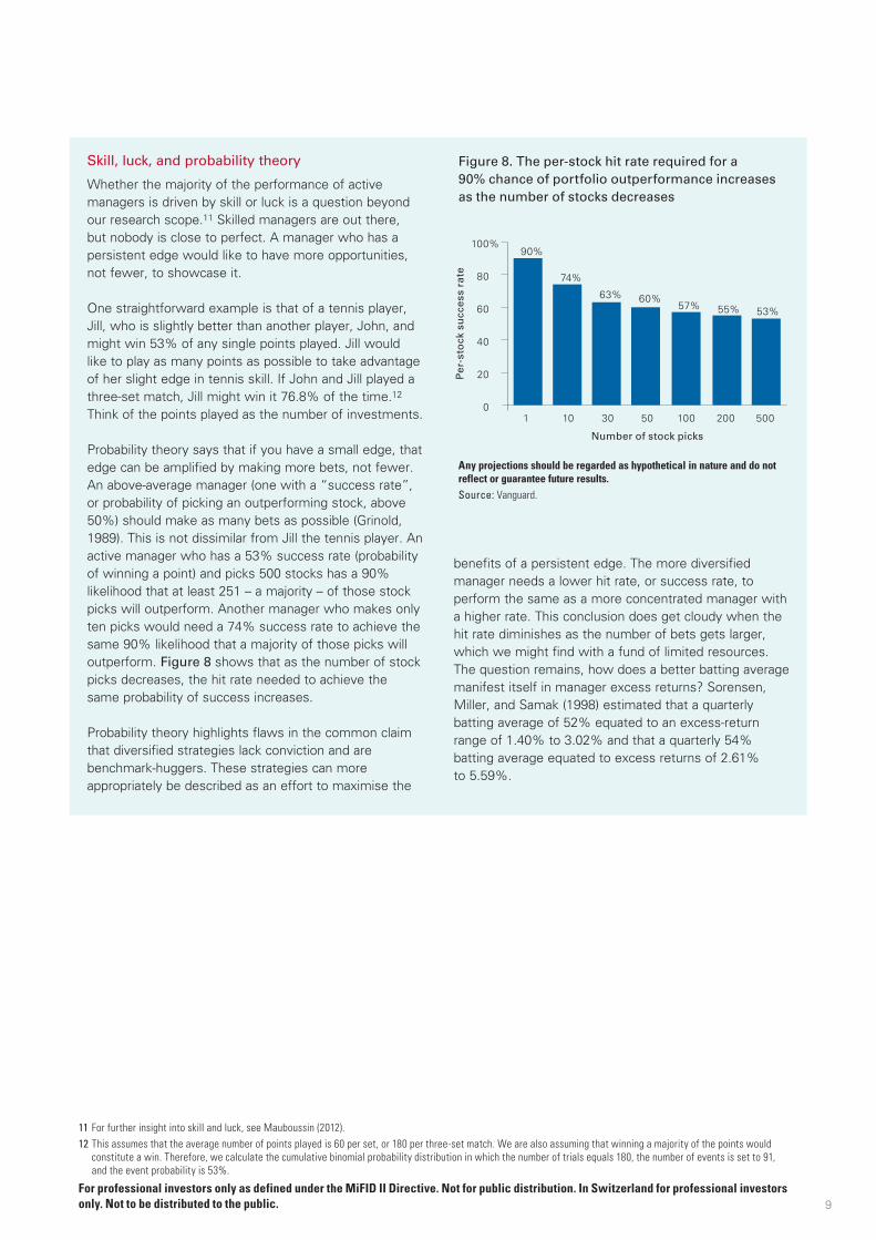
Skill, luck, and probability theory

Whether the majority of the performance of active managers is driven by skill or luck is a question beyond our research scope.11 Skilled managers are out there, but nobody is close to perfect. A manager who has a persistent edge would like to have more opportunities, not fewer, to showcase it.

One straightforward example is that of a tennis player, Jill, who is slightly better than another player, John, and might win 53% of any single points played. Jill would like to play as many points as possible to take advantage of her slight edge in tennis skill. If John and Jill played a three-set match, Jill might win it 76.8% of the time.12 Think of the points played as the number of investments.

Probability theory says that if you have a small edge, that edge can be amplified by making more bets, not fewer. An above-average manager (one with a “success rate”, or probability of picking an outperforming stock, above 50%) should make as many bets as possible (Grinold, 1989). This is not dissimilar from Jill the tennis player. An active manager who has a 53% success rate (probability of winning a point) and picks 500 stocks has a 90% likelihood that at least 251 – a majority – of those stock picks will outperform. Another manager who makes only ten picks would need a 74% success rate to achieve the same 90% likelihood that a majority of those picks will outperform. Figure 8 shows that as the number of stock picks decreases, the hit rate needed to achieve the same probability of success increases.

Probability theory highlights flaws in the common claim that diversified strategies lack conviction and are benchmark-huggers. These strategies can more appropriately be described as an effort to maximise the

benefits of a persistent edge. The more diversified manager needs a lower hit rate, or success rate, to perform the same as a more concentrated manager with a higher rate. This conclusion does get cloudy when the hit rate diminishes as the number of bets gets larger, which we might find with a fund of limited resources. The question remains, how does a better batting average manifest itself in manager excess returns? Sorensen, Miller, and Samak (1998) estimated that a quarterly batting average of 52% equated to an excess-return range of 1.40% to 3.02% and that a quarterly 54% batting average equated to excess returns of 2.61% to 5.59%.

Figure 8. The per-stock hit rate required for a 90% chance of portfolio outperformance increases as the number of stocks decreases

Any projections should be regarded as hypothetical in nature and do not reflect or guarantee future results.Source: Vanguard.

0

20

40

60

80

100%

Per

-sto

ck s

ucc

ess

rate

1

90%

74%

10

63% 60%

30 50

57%

100 200

55%

500

53%

0

10

20

30

40

50

60

70

80%

Axi

s la

bel

if n

eed

ed

Number of stock picks

10

13 This is just one potential definition of success. Different definitions (for example, the probability of selecting any of the top 10% performing stocks, or of avoiding the worst 20% performing stocks) would lead to different results. It is also important to stress that the stocks in the top or bottom 50% set can be selected with equal probability. This means an investor with a higher success rate will be able to pick a top-performing stock with, for example, a 52% probability; however, any of the top-performing stocks will have the same chance of being selected.


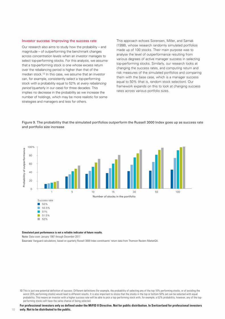
Investor success: Improving the success rate

Our research also aims to study how the probability – and magnitude – of outperforming the benchmark changes across concentration levels when an investor manages to select top-performing stocks. For this analysis, we assume that a top-performing stock is one whose excess return over the rebalancing period is higher than that of the median stock.13 In this case, we assume that an investor can, for example, consistently select a top-performing stock with a probability equal to 52% at every rebalancing period (quarterly in our case) for three decades. This implies no decrease in the probability as we increase the number of holdings, which may be more realistic for some strategies and managers and less for others.

This approach echoes Sorensen, Miller, and Samak (1998), whose research randomly simulated portfolios made up of 100 stocks. Their main purpose was to analyse the level of outperformance resulting from various degrees of active manager success in selecting top-performing stocks. Similarly, our research looks at changing the success rates, and computing return and risk measures of the simulated portfolios and comparing them with the base case, which is a manager success equal to 50% (that is, random stock selection). Our framework expands on this to look at changing success rates across various portfolio sizes.

Figure 9. The probability that the simulated portfolios outperform the Russell 3000 Index goes up as success rate and portfolio size increase


0

20

40

60

80

100%

50%50.5%51%51.5%52%

Success rate

Pro

bab

ility

of

ou

tper

form

ance

1 5 10 15 30 50 100


11

14 The difference in results is explained by random sampling approximation.


To understand our results’ sensitivity to the success rate, we chose five success rates at increments of 0.5%, starting from the base-case success rate up to 52%. Assuming a success rate equal to 50% implies that both top- and bottom-performing stocks can be picked with the same probability. Therefore, our results will be very close to those shown in the previous sections.14

Figure 9 shows that both higher success rates and greater diversification are associated with a higher probability of outperformance. In our simulation, however, diversification seems to have a more powerful impact. Even at a 52% success rate, the five-stock portfolio barely has a greater than 50% chance of

outperforming. In a 100-stock portfolio, by contrast, this same success rate yields an almost 100% probability of outperforming.

In Figure 10, we report the expected excess return of portfolios simulated with various success rates. These results help us answer the following question: what is the success-rate level needed to achieve a specific excess return target for a given portfolio size? For a five-stock portfolio, a success rate as high as 52% is needed to have a positive expected performance at the end of the entire investment horizon. As we add more stocks to the portfolio, the success rate needed to outperform

Figure 10. The average expected excess return rises as success rate and portfolio size increase


-10

-8

-6

-4

-2

0

2

4%

50%50.5%51%51.5%52%

Success rate

Ave

rag

e ex

pec

ted

exc

ess

retu

rn

1 5 10 15 30 50 100


12

15 Although we tested funds with fewer than ten holdings in our bottom-up simulations, either they were funds-of-funds or the holdings were not individual stocks.16 We ran the Durbin-Wu-Hausman test to verify the potential benefit of using a random effects model. (This test assesses the consistency of an estimator when

compared with a less efficient consistent estimator [Greene, 1997]; the test is often used for panel data analysis to choose between fixed effects and random effects models.) Our findings fail to reject the null hypothesis, suggesting that a time–random effects model should be preferred. However, the results following this approach are not quantitatively different from those following our time–fixed effects model.

17 We use the Russell 3000 Index, rather than the primary prospectus benchmark, as the equity benchmark to allow for consistency among funds. Also, to perform the sector concentration and factor concentration data analysis, we need a unique and homogeneous market benchmark. We consider the Russell 3000 Index to be an appropriate and widely accepted benchmark for US equities.


decreases. In fact, for portfolios with 30 or more stocks, any success rate higher than 50% considered in our analysis would lead to an excess return higher than zero.

Overall, the results show that holding a more diversified portfolio helps increase the chances of outperforming the benchmark and achieving higher average returns. Investors who seek to outperform above certain excess return thresholds will improve their chances by reducing the number of holdings but will experience a more rapid increase in the chance of underperforming. Lastly, the benefits of diversification are present and potentially amplified in the case of an investor who can consistently pick top-performing stocks.

Historical approach to analysing the concentration within portfolios

So far we have evaluated concentration based on simulated analysis using historical equity return data. In this section, we investigate, through historical fund performance, whether a relationship exists between active equity funds’ excess returns and their concentration. We conduct panel data regression to see how much of excess return variance is explained by number of holdings while controlling for other variables, including sector and factor concentration.

These controls are important because having a large number of stocks in a portfolio does not necessarily imply low concentration. A significant fraction of the holdings might come from the same industry sector (such as financials or technology) or have similar factor exposure (such as value or small-cap bias). The results yield two notable insights. First, there is a positive and highly significant relationship between the number of holdings and net excess returns. The more holdings, on average, the higher the excess returns. Second, there is a negative and highly significant relationship between the number of holdings and fund expense ratios. On average, more concentrated funds cost more. We now review the data and methodology in detail.

Data and methodology

We collected active US equity funds’ quarterly data from January 2000 to December 2017 from Morningstar, Inc. We selected only funds available for sale in the United States. Similar to Kacperczyk, Sialm, and Zheng (2005) and Goldman, Sun, and Zhou (2016), we also limited our dataset to one share class per fund to make sure that multiple-share-class funds were not overweighted in our analysis. Lastly, funds-of-funds and funds with fewer than ten holdings were excluded.15 Ultimately, after adjustments, our final dataset includes 2,136 funds.

We define number of stock holdings as the number that a fund held at the beginning of each measurement period and analyse the impact of that number on fund excess returns. For the panel data analysis, we specify an unbalanced time-fixed effects model in which we regress the funds’ excess returns using the Russell 3000 Index as the relevant benchmark in each quarter on the number of holdings, the Sector Concentration Index (SCI), the Factor Concentration Index (FCI), and a set of control variables.16,17 We believe the introduction of “time effects” allows us to better account for shared factors and business-cycle events that might affect all funds. This ultimately leads us to define the following variables:

• Net ExcRet is the net excess return of any fund.

• Ln(Age) is the natural log of fund age.

• Expense is the fund expense ratio.

• Turnover is annualised fund turnover.

• Ln(TNA) is the natural log of fund total net assets.

• Ln(NumHold) is the natural log of number of fund stock holdings.

• SCI is the fund sector index as specified in Appendix I, on page 17.

• FCI is the factor concentration index as specified in Appendix I, on page 17.

13

18 Prior research is mixed on whether to take the natural logarithm of portfolio turnover when portfolio turnover is being used as a control variable. We tested our model using both methods with similar results.

19 For further details, see Greene (1997).20 We addressed other potential model specifications, including the removal of age or TNA or both, with quantitatively similar results.21 The number of observations is considerably larger (over 100,000) than previous studies because of a combination of factors – namely, the number of funds, the time

period, and the data frequency (such as quarterly observations versus annual observations). For instance, Kacperczyk, Sialm, and Zheng (2005) used a dataset with roughly 35,000 observations depending on the test and regressions performed. Brands, Brown, and Gallagher’s (2005) sample size was approximately 1,200 observations, and Goldman, Sun, and Zhou’s (2016) dataset considered 34,176 observations. This has the advantage of making our coefficient estimates more reliable but leads us to easily reject the null hypothesis for relationships that are not necessarily economically significant (Lin, Lucas, and Shmueli, 2013).


Since most of our variables show some level of positive skewness with a few of the variables significantly affected by extreme values, we take the natural logarithm of the funds’ age, total net assets, and number of holdings in order to linearise their relationship with excess return.18 To alleviate the potential impact of endogeneity, we lagged all independent variables by one quarter. Also, for robustness, we estimate our model using Restricted Maximum Likelihood Estimation (REML):19

Net ExcReti,t = α + β1Ln(Age)i,t-1 + β2Expensei,t-1 + β3Turnoveri,t-1 + β4Ln(TNA)i,t-1 + β5Ln(NumHold)i,t-1 + β6SCIi,t-1 + β7 FCIi,t-1+μt-1 + εi,t-1

Although our methodology is based on literature such as Kacperczyk, Sialm, and Zheng (2005); Brands, Brown, and Gallagher (2005); Huij and Derwall (2011); and Goldman, Sun, and Zhou (2016), our approach differs in three main aspects:

• We explicitly take into account in the panel model the number of holdings.

• We control for factor and sector concentration using consistent definitions, and we include factor concentration as a control variable rather than using factor-adjusted funds’ alpha as the dependent variable.

• Our data sample is significantly larger than that of previous studies, making our results more statistically accurate.

Summary statistics and results

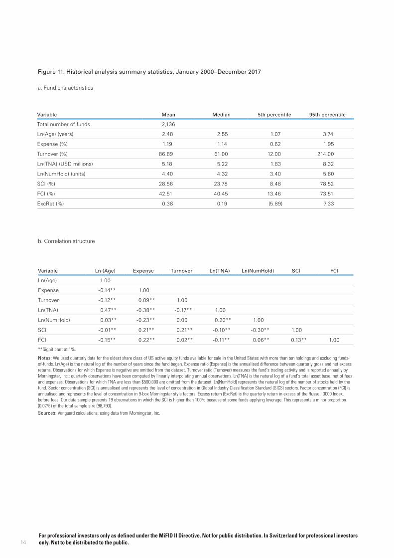
Figure 11a, on page 14, documents the summary statistics for natural log number of holdings, sector concentration, factor concentration, and other fund characteristics. The mutual funds in our sample vary widely in their characteristics (for the non-log fund characteristics, see Appendix II on page 18). Figure 11b shows the contemporaneous correlations between the independent variables used in our model. On average, the correlation between age and TNA is positive, as we might expect given that older funds tend to have acquired more assets than younger funds. We also note that expense ratio has a positive correlation with factor and sector concentration but a negative correlation with number of holdings. Overall, our dataset summary statistics are consistent with previous studies (such as Kacperczyk, Sialm, and Zheng, 2005, and Goldman, Sun, and Zhou, 2016).

Figure 12, on page 15, summarises our findings for different models’ specifications with and without accounting for the effects of sector and factor concentration.20 The first point to notice is that most of our estimates are statistically significant at a 1% level.21 The R-squared figures for our model specifications might appear weak at first glance, but the amount of unexplained variance is not surprising. The low R-squared is to be expected for active equity funds and does not invalidate the significance of the explanatory variables.

14

Figure 11. Historical analysis summary statistics, January 2000–December 2017

a. Fund characteristics

Variable Mean Median 5th percentile 95th percentile

Total number of funds 2,136

Ln(Age) (years) 2.48 2.55 1.07 3.74

Expense (%) 1.19 1.14 0.62 1.95

Turnover (%) 86.89 61.00 12.00 214.00

Ln(TNA) (USD millions) 5.18 5.22 1.83 8.32

Ln(NumHold) (units) 4.40 4.32 3.40 5.80

SCI (%) 28.56 23.78 8.48 78.52

FCI (%) 42.51 40.45 13.46 73.51

ExcRet (%) 0.38 0.19 (5.89) 7.33

b. Correlation structure

Variable Ln (Age) Expense Turnover Ln(TNA) Ln(NumHold) SCI FCI

Ln(Age) 1.00

Expense -0.14** 1.00

Turnover -0.12** 0.09** 1.00

Ln(TNA) 0.47** -0.38** -0.17** 1.00

Ln(NumHold) 0.03** -0.23** 0.00 0.20** 1.00

SCI -0.01** 0.21** 0.21** -0.10** -0.30** 1.00

FCI -0.15** 0.22** 0.02** -0.11** 0.06** 0.13** 1.00

**Significant at 1%.

Notes: We used quarterly data for the oldest share class of US active equity funds available for sale in the United States with more than ten holdings and excluding funds-of-funds. Ln(Age) is the natural log of the number of years since the fund began. Expense ratio (Expense) is the annualised difference between quarterly gross and net excess returns. Observations for which Expense is negative are omitted from the dataset. Turnover ratio (Turnover) measures the fund’s trading activity and is reported annually by Morningstar, Inc.; quarterly observations have been computed by linearly interpolating annual observations. Ln(TNA) is the natural log of a fund’s total asset base, net of fees and expenses. Observations for which TNA are less than $500,000 are omitted from the dataset. Ln(NumHold) represents the natural log of the number of stocks held by the fund. Sector concentration (SCI) is annualised and represents the level of concentration in Global Industry Classification Standard (GICS) sectors. Factor concentration (FCI) is annualised and represents the level of concentration in 9-box Morningstar style factors. Excess return (ExcRet) is the quarterly return in excess of the Russell 3000 Index, before fees. Our data sample presents 19 observations in which the SCI is higher than 100% because of some funds applying leverage. This represents a minor proportion (0.02%) of the total sample size (98,790).Sources: Vanguard calculations, using data from Morningstar, Inc.


15

22 The coefficient of turnover is consistent with Kacperczyk, Sialm, and Zheng (2005); Goldman, Sun, and Zhou (2016); and Brands, Brown, and Gallagher (2005), while fund age and total net assets are consistent with Brands, Brown, and Gallagher.


Figure 12. Panel data regression: Time–fixed effects on net excess returns

Coefficient NumHold NumHold + SCI NumHold + FCI NumHold + SCI + FCI

Ln(NumHold) 9.49** 16.06** 4.24** 10.32**

Control Variables

Ln(Age) 4.60* 2.92 8.85** 8.38**

Expense –50.94** –74.27** –116.85** –133.94**

Turnover –0.05** –0.08** -0.05** –0.07**

Ln(TNA) –8.88** –8.74** –8.83** –9.13**

SCI 1.01** 0.82**

FCI 1.45** 1.36**

Adjusted R2 8.46% 8.77% 9.01% 9.11%

Past performance is not a reliable indicator of future results.

Notes: We used quarterly data for the oldest share class of US active equity funds available for sale in the United States with more than ten holdings and excluding funds-of-funds. Observations for which Expense is negative or TNA is less than $500,000 are omitted from the data sample. All regressions include time dummies. One star indicates significance at the 5% level; two stars indicate significance at the 1% level. Fund age (Age) is in years; expense ratio (Expense) is in percentage points; turnover ratio (Turnover), sector concentration (SCI), and factor concentration (FCI) are in percentage points; total net assets (TNA) is in millions of US dollars; and number of holdings (NumHold) is in units.Sources: Vanguard calculations, using data from Morningstar, Inc.

The coefficient of number of holdings is statistically significant at least at 5% across all model specifications and is economically significant and positive, suggesting that given any specified level of sector or factor concentration, a fund’s performance improves with a higher number of holdings. This finding is consistent with Goldman, Sun, and Zhou (2016). For example, based on Figure 12, increasing holdings by 10 percent leads to an increase of 3.80 basis points (bps) in annual excess returns (9.49 x 10% x 4). When we consider the impact of both sector and factor exposures in the fourth column of Figure 12, using the same 10% increase in holdings, a slightly higher coefficient of 10.32 leads to an increase of 4.13 bps in annual excess returns.

Consistent with Rowley, Harbron, and Tufano (2017), on average, expense ratio has a statistically significant negative impact on performance, and the coefficients of

the other control variables (turnover, fund age, and total net assets) are somewhat mixed relative to findings in previous studies.22

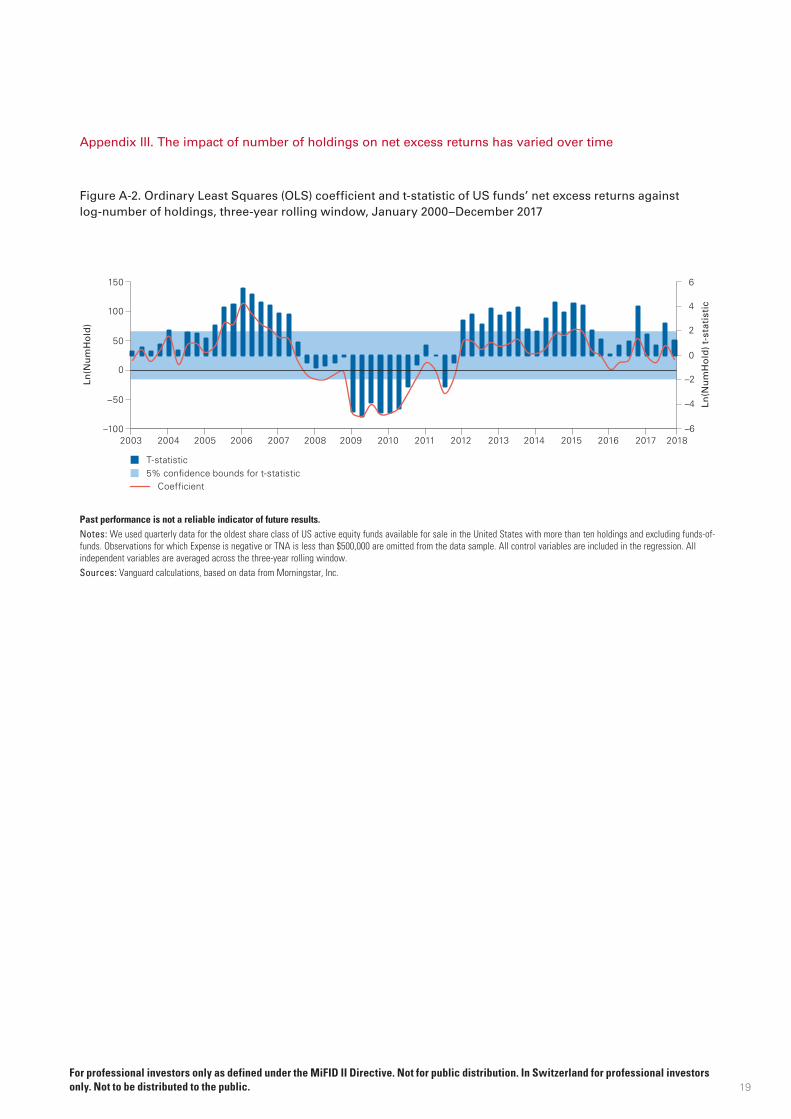
Lastly, the time–fixed effects model specified above allows for a change in the constant (α) across time but does not map any dynamic change in the beta-coefficients. Additional analysis (see Appendix III on page 19) does show that the effect of concentration (measured by number of holdings) on excess return has fluctuated considerably over time. This is consistent with Hickey et al. (2017), who found that US large-cap equity funds with fewer holdings had historically slightly higher returns but that this was largely driven by short time windows in the late 1990s and early 2000s, and we found similar time-period-specific outperformance by concentrated funds. The overall impact of number of holdings on US equity active funds’ excess returns is positive but episodically has turned negative.

16

23 A full assessment of the optimal sizing of portfolios based on investors’ goals and preferences should be explored in further research.For professional investors only as defined under the MiFID II Directive. Not for public distribution. In Switzerland for professional investors only. Not to be distributed to the public.

Implications for investors and further research

As with all investments, one should expect premiums if taking on more risk. Common examples include equity versus fixed income, corporate bonds versus government bonds, and high-yield bonds versus investment-grade bonds. We found that less diversified portfolios have more relative risk than more diversified ones and that investors should therefore expect higher returns from the less diversified portfolios, but the evidence from our bottom-up simulations shows that concentrated portfolios of randomly selected stocks have lower average returns than diversified portfolios. Our historical analysis is consistent with these theoretical results, finding lower average returns for the less diversified portfolios. Our results suggest that a concentrated manager creates more opportunity for outsized excess returns (either positive or negative), although as we decrease the number of holdings, the chance of underperformance increases at a faster rate than the chance of outperforming.

The mere function of being less diversified via random selection makes for a performance hurdle that portfolio managers must overcome.23 So one must find talented active managers with the ability to overcome this hurdle (along with typically higher fees). Those managers who can select a concentrated portfolio of “home run” stocks have the potential to earn extreme positive returns. The question is whether they can reliably and consistently identify those stocks in advance. This analysis yields valuable tools for manager evaluation: excess return hurdles or success-rate hurdles that can be used in conjunction with well-established determinants of success such as cost.

Conclusion

Historical cumulative returns of individual stocks are skewed whereby overall market returns are determined by a small minority of stocks. Therefore, all else being equal, a more diversified portfolio is more likely to hold these outperforming stocks while displaying a lower dispersion of portfolio returns. We conducted simulations of various portfolio sizes and showed that those portfolios with fewer holdings underperformed those with more holdings, leading to a higher return hurdle to overcome. Understanding that some investors may prefer to generate returns above a certain excess return

target, we found that decreasing the number of holdings increased the chance of outperformance but came with an even higher probability of underperformance by the same excess return target. In addition, investors who believe their stock-selection ability is better than chance would be best served applying that skill by selecting more stocks, not fewer. Finally, we tested mutual fund performance as a function of various levels of portfolio concentration as measured by number of holdings and found that, historically, increased diversification yielded higher returns.

References

Bessembinder, Hendrik, 2018. Do Stocks Outperform Treasury Bills? Journal of Financial Economics (Forthcoming).

Brands, Simone, Stephen J. Brown, and David R. Gallagher, 2005. Portfolio Concentration and Investment Manager Performance. International Review of Finance 5(3-4): 149–174.

Cembalest, Michael, 2014. The Agony and the Ecstasy: The Risks and Rewards of a Concentrated Stock Position. Eye on the Market: Special Edition. J.P. Morgan Asset Management.

Cohen, Randolph B., Christopher Polk, and Bernhard Silli, 2010. Best Ideas. Working Paper. London: Paul Woolley Centre, The London School of Economics.

Cremers, K.J. Martijn, and Antti Petajisto, 2009. How Active Is Your Fund Manager? A New Measure That Predicts Performance. The Review of Financial Studies 22(9): 3329–3365.

Edwards, Tim, and Craig J. Lazzara, 2016. Fooled by Conviction. Index Investment Strategy, S&P Dow Jones Indices.

Evans, John L., and Stephen H. Archer, 1968. Diversification and the Reduction of Dispersion: An Empirical Analysis. The Journal of Finance 23(5): 761–767.

Fisher, Lawrence, and James H. Lorie, 1970. Some Studies of Variability of Returns on Investments in Common Stocks. The Journal of Business 43(2): 99–134.

Goldman, Eitan, Zhenzhen Sun, and Xiyu (Thomas) Zhou, 2016. The Effect of Management Design on the Portfolio Concentration and Performance of Mutual Funds. Financial Analysts Journal 72(4): 49–61.

Graham, Benjamin, 1949. The Intelligent Investor, first edition. New York, N.Y.: Harper & Brothers.

17

Greene, William H., 1997. Econometric Analysis, third edition. Upper Saddle River, N.J.: Prentice-Hall.

Grinold, Richard C., 1989. The Fundamental Law of Active Management. The Journal of Portfolio Management 15(3): 30–37.

Heaton, J.B., N.G. Polson, and J.H. Witte, 2017. Why Indexing Works. Applied Stochastic Models in Business and Industry 33(6): 690–693.

Hickey, Michael, Christopher Luongo, Darby Nielson, and Zhitong Zhang, 2017. Does the Number of Stocks in a Portfolio Influence Returns? Fidelity Investments.

Huij, Joop, and Jeroen Derwall, 2011. Global Equity Fund Performance, Portfolio Concentration, and the Fundamental Law of Active Management. Journal of Banking & Finance 35(1): 155–165.

Ikenberry, David L., Richard L. Shockley, and Kent L. Womack, 1998. Why Active Fund Managers Often Underperform the S&P 500: The Impact of Size and Skewness. The Journal of Private Portfolio Management 1: 13–26.

Kacperczyk, Marcin, Clemens Sialm, and Lu Zheng, 2005. On the Industry Concentration of Actively Managed Equity Mutual Funds. The Journal of Finance 60(4): 1983–2011.

Lin, Mingfeng, Henry C. Lucas Jr., and Galit Shmueli, 2013. Too Big to Fail: Large Samples and the p-Value Problem. Information Systems Research 24(4): 906–917.

Malkiel, Burton, 1973. A Random Walk Down Wall Street, first edition. New York, N.Y.: W.W. Norton & Company.

Mauboussin, Michael J., 2012. The Success Equation: Untangling Skill and Luck in Business, Sports, and Investing. Boston, Mass.: Harvard Business Review Press.

Rowley, James J., Garrett L. Harbron, and Matthew C. Tufano, 2017. In Pursuit of Alpha: Evaluating Active and Passive Strategies. Valley Forge, Pa.: The Vanguard Group.

Sorensen, Eric H., Keith L. Miller, and Vele Samak, 1998. Allocating Between Active and Passive Management. Financial Analysts Journal 54(5): 18–31.

Statman, Meir, 2004. The Diversification Puzzle. Financial Analysts Journal 60(4): 44–53.

Yeung, Danny, Paolo Pellizzari, Ron Bird, and Sazali Abidin, 2012. Diversification Versus Concentration … and the Winner Is? Working Paper Series 18. Sydney, Australia: Paul Woolley Centre for the Study of Capital Market Dysfunctionality, University of Technology.

Appendix I. Defining sector and factor concentration

Similar to what was previously done by Brands, Brown, and Gallagher (2005), Kacperczyk, Sialm, and Zhang (2005), and Goldman, Sun, and Zhou (2016), we define the Sector Concentration Index (SCI) at any point in time for any fund (i) as:

SCIi = 1/2 ∑ |wi,GICS – wR3000,GICS |

A fund’s sector concentration is therefore the sector active share (Cremers and Petajisto, 2009) compared with the relative sector weight of the Russell 3000 Index, which we use as the benchmark. For our analysis, we use the 11 GICS industry sectors as at 31 December 2017: consumer discretionary, consumer staples, energy, financials, health care, industrials, information technology, materials, real estate, telecommunication services, and utilities.

We follow a similar approach for the Factor Concentration Index (FCI):

FCIi = 1/2 ∑ |wi,factor – wR3000,factor |

We define a fund’s factor concentration as the 9-box Morningstar style factor active share compared with the relative weight of the Russell 3000 Index. These are: small-cap value, mid-cap value, large-cap value, small-cap blend, mid-cap blend, large-cap blend, small-cap growth, mid-cap growth, and large-cap growth.

We prefer active share to other active management measures such as the Industry Concentration Index or the Herfindahl index primarily because active share has a direct and intuitive economic interpretation. With no short positions, active share is defined such that it can range from 0% to 100%, where 0% represents perfectly matching the benchmark and 100% represents a portfolio with no overlap at all. Also, as pointed out by Cremers and Petajisto (2009), the Industry Concentration Index is a hybrid measure. sharing features of both active share and tracking error.

11

GICS=1

9

factor=1


18

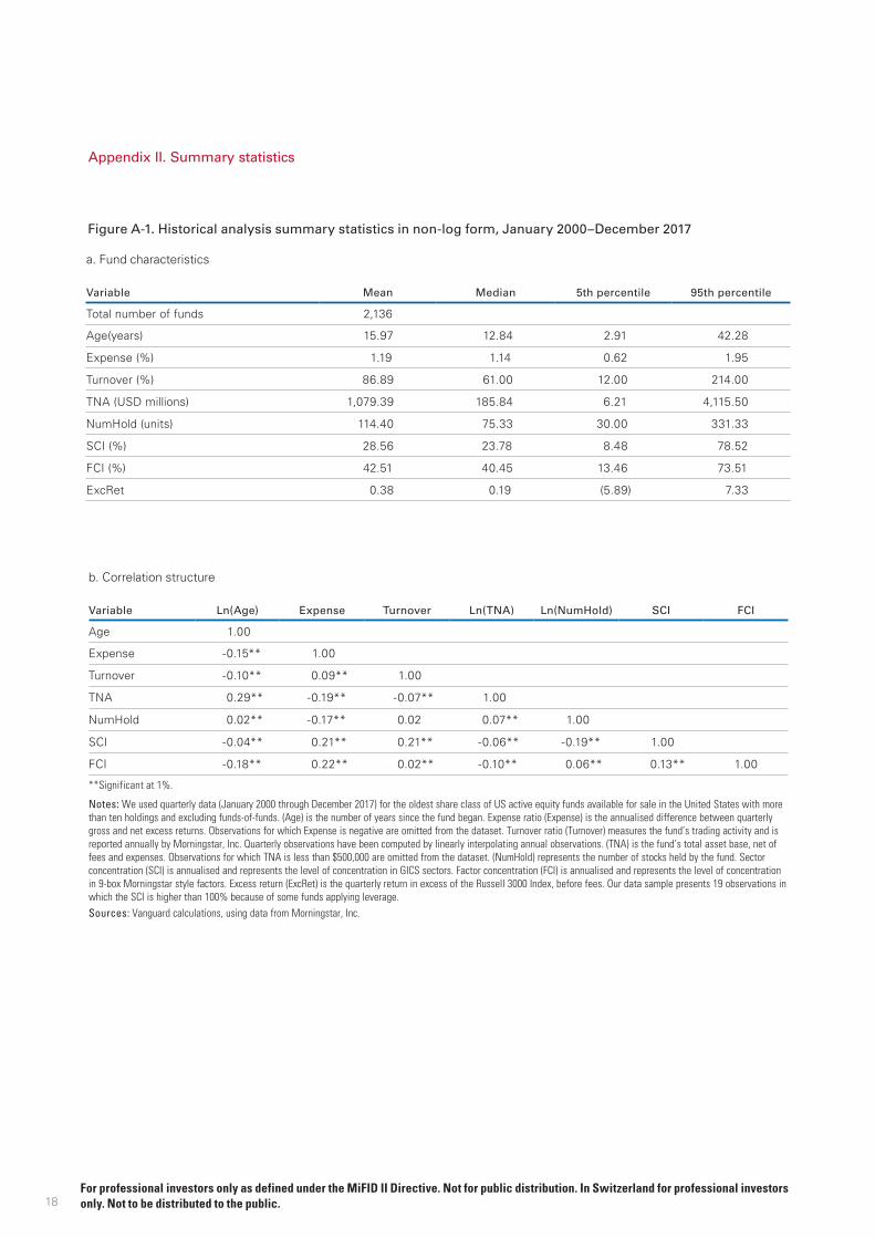
Appendix II. Summary statistics

Figure A-1. Historical analysis summary statistics in non-log form, January 2000–December 2017

a. Fund characteristics

Variable Mean Median 5th percentile 95th percentile

Total number of funds 2,136

Age(years) 15.97 12.84 2.91 42.28

Expense (%) 1.19 1.14 0.62 1.95

Turnover (%) 86.89 61.00 12.00 214.00

TNA (USD millions) 1,079.39 185.84 6.21 4,115.50

NumHold (units) 114.40 75.33 30.00 331.33

SCI (%) 28.56 23.78 8.48 78.52

FCI (%) 42.51 40.45 13.46 73.51

ExcRet 0.38 0.19 (5.89) 7.33

b. Correlation structure

Variable Ln(Age) Expense Turnover Ln(TNA) Ln(NumHold) SCI FCI

Age 1.00

Expense -0.15** 1.00

Turnover -0.10** 0.09** 1.00

TNA 0.29** -0.19** -0.07** 1.00

NumHold 0.02** -0.17** 0.02 0.07** 1.00

SCI -0.04** 0.21** 0.21** -0.06** -0.19** 1.00

FCI -0.18** 0.22** 0.02** -0.10** 0.06** 0.13** 1.00

**Significant at 1%.

Notes: We used quarterly data (January 2000 through December 2017) for the oldest share class of US active equity funds available for sale in the United States with more than ten holdings and excluding funds-of-funds. (Age) is the number of years since the fund began. Expense ratio (Expense) is the annualised difference between quarterly gross and net excess returns. Observations for which Expense is negative are omitted from the dataset. Turnover ratio (Turnover) measures the fund’s trading activity and is reported annually by Morningstar, Inc. Quarterly observations have been computed by linearly interpolating annual observations. (TNA) is the fund’s total asset base, net of fees and expenses. Observations for which TNA is less than $500,000 are omitted from the dataset. (NumHold) represents the number of stocks held by the fund. Sector concentration (SCI) is annualised and represents the level of concentration in GICS sectors. Factor concentration (FCI) is annualised and represents the level of concentration in 9-box Morningstar style factors. Excess return (ExcRet) is the quarterly return in excess of the Russell 3000 Index, before fees. Our data sample presents 19 observations in which the SCI is higher than 100% because of some funds applying leverage.Sources: Vanguard calculations, using data from Morningstar, Inc.


19

Appendix III. The impact of number of holdings on net excess returns has varied over time

Figure A-2. Ordinary Least Squares (OLS) coefficient and t-statistic of US funds’ net excess returns against log-number of holdings, three-year rolling window, January 2000–December 2017

Past performance is not a reliable indicator of future results.Notes: We used quarterly data for the oldest share class of US active equity funds available for sale in the United States with more than ten holdings and excluding funds-of-funds. Observations for which Expense is negative or TNA is less than $500,000 are omitted from the data sample. All control variables are included in the regression. All independent variables are averaged across the three-year rolling window.Sources: Vanguard calculations, based on data from Morningstar, Inc.

Ln(N

um

Ho

ld)

150

2003–6

–4

–2

0

2

4

6

Ln(N

um

Ho

ld)

t-st

atis

tic

100

50

0

–50

–1002004 2005 2006 2007 2008 2009 2010 2011 2012 2013 2014 2015 2016 2017 2018

T-statistic5% confidence bounds for t-statistic

Coefficient


© 2018 The Vanguard Group, Inc. All rights reserved. VAM 739585 VISG 739587

ISGITO_E 022019

Connect with Vanguard® > global.vanguard.com

CFA® is a registered trademark owned by CFA Institute.


Documents

How to increase the odds of owning the few stocks that ... · portfolio’s number of randomly selected stocks, investors are more likely to include those stocks with higher magnitudes