How to iFlow

Kyongryun Lee, Nishant Gopalakrishnan, and Chao-Jen Wong

April 22, 2010

1 Introduction

The iFlow package [3] is implemented using the Gtk2 toolkit [2, 4], and sits on top of Rand Bioconductor. It allows convenient management, visualization, and analysis of flowcytometry (FCM) data.

Integrated with several FCM related packages1 in Bioconductor, iFlow provides aninteractive graphical user interface (GUI) allowing users to facilitate the analysis andvisualization of complex FCM data. The user can find the major tools on main applica-tion window (see Figure 1): the Data menu allows manipulation of the loaded data; theGraphic menu provides a range of visualization methods; and the Gate MENU supportsa number of automated gating algorithms as well as manual gating.

This vignette provides a step-by-step demonstration of a typical work flow for FCManalysis and guidelines for all the tools and methods available in iFlow. We start byloading a sample data, GvHD, in the flowCore package and showing how to view thecorresponding parameters and annotation data. We proceed to transform the datasetwith the arcsinh transformation, followed by per-channel basis normalization on someof the flow channels. A couple of visualization functions are then demonstrated for thecurrently active dataset. Finally, we illustrate how to create gating objects by manualor auto-gating methods and show how to apply these objects to the active dataset.

2 Installation

The iFlow package can be installed by typing in the following lines into an R console.

> source("http://bioconductor.org/biocLite.R")

> biocLite("iFlow")

iFlow can be started using library(iFlow)

1These include the flowCore, flowStats, flowViz packages so far. In the future, we hope to includenovel analytic methods implemented in other Bioconductor packages such as flowClust, flowMerge andetc.

1

Menu Description

File- Open Loads FCS or rda (rdata) files.- Save As Saves statistics for data.- Load Loads FCS or rda (rdata) files internally.- Quit Closes iFlow.

Data- Transformation Transforms data in linear, ln, log, biexponential,

logicle, arcsinh, and quadratic functions.- Subset- - Filters Makes a subset with a selected gate object.- - pData Makes a subset with selected sample covariates.- Compensation Compensates data by applying a provided

spillover matrix (limited currently).- Normalization Normalizes data through provided three functions :

warpSet, gpaSet, gaussNorm.- Summary Summaries data through basic statistics :

median, mean, max, min, or user-defined function.

Graphics- Plots Provides various plots for flowSet and flowFrame.

Displays data in the form of, Contour, ECDF, Dot, Histogram,Parallel Coordinate, Q-Q, Scatter Plot Matrix, Smooth Scatter,Stack Density, Timeline and Workflow.

Gate- Create Creates an object by provided gating methods :

Rectangle, Quadrant, Lymphcyte, Kmeans, Norm2,Curv1, Curv2, and manual gating.

- Combine Runs boolean operations to combine objects: &, | and !.

- Backgating Shows the effect of the gate on each level in a gating hierarchy.ProBin- ProBin Visualizes the differences between the binned control and data.

Help Supports documentation and command history for users.

Table 1: The main application menus.

2

Figure 1: iFlow’s main application window.

3 Main Application

Upon calling up the iFlow package, the iFlow main application window will appear onthe screen, as depicted in Figure 1. The application window consists of a control and amain panel. The control panel lists all the loaded datasets and defined gates, and allowsthe user to select one of interest. All operations are performed on the currently selecteddataset. The main panel consists of a notebook with three types of tabs:

Information Provides details about the currently selected dataset. It also displaysinformation about previously defined gates and transformations, which can bereused in other tasks.

Annotation Provides phenotypic information about the individual samples in the cur-rent dataset.

Summary Provides various summaries of the currently selected dataset.

The application consists of File, Data, Graphics, Gate, ProBin and Help menu sec-tions with each providing detailed sub menu items. The functionality provided by eachmenu is described in detail in the following sections.

3.1 File Menu

The File menu provides options to import and export data from into the iFlow program.The File menu has four sub menus Open, Load, Save As and Quit. The Open option

3

Figure 2: An iFlow graphics window displaying data of three FCM channels in the formof stacked density plots for ten different samples.

can be used to import data available as FCS or LMD files while the Load option allowsthe user to conveniently load flow cytometry data already available in the R globalworkspace.

The GvHD data available in the flowCore package can be imported into iFlow byfirst reading it into the R workspace using the following lines of code and subsequentlyusing the Load menu to select the GvHD3 and GvHD5 flowSets that were created, asdemonstrated in Figure 3.

> data(GvHD)

> GvHD3 <- GvHD[1:3]

> GvHD5 <- GvHD[5:10]

The data panel displays the GvHD3 and GvHD5 flowSets that have been loadedin the iFlow program. More details regarding the datasets GvHD3 and GvHD5 can beobtained by first selecting a flowSet and then accessing the Information and Annotationpanels. The Information panel provides details regarding the fluorescence stains thatwere used (Figure 4) while the Annotation panel provides a tabular view of the samplecovariates (PatientID, Visit number etc.) (Figure 5)

4

Figure 3: A pop-up GUI for selecting the imported datasets.

Figure 4: Information tab showing the details of the currently selected dataset, GvHD3.

5

Figure 5: Annotation tab showing phenotypic information of the GvHD3 dataset.

6

Figure 6: The arcsinh transformation GUI.

3.2 Data Menu

The Data menu provides options to transform, subset, compensate or normalize datathat is currently selected in the data panel.

3.2.1 Transformation

The dataset selected by the user can be transformed for better visualization of the datausing the Transformation option available in the Data menu. The iFlow package provideslinear, log, ln, logicle, arcsinh, biexponential scale and quadratic transforma-tions. The user is also provided the option of applying the transformation of choice toselected fluorescence channels in the dataset.

Continuing with our example, we proceed to transform the GvHD3 dataset withthe arcsinh transformation. The results is shown in Figure 6. The GvHD3 objectafter transformation can be observed in the Data panel as GvHD3 trans, as depicted inFigure 7

3.2.2 Subset

The subset option allows the user to subset the selected dataset in the Data panelusing either a gate or by making use of sample covariates that are displayed under theAnnotation tab.

We proceed to subset the transformed data by the sample covariate name to includetwo samples s5a02 and s5a03, as illustrated in Figure 8

7

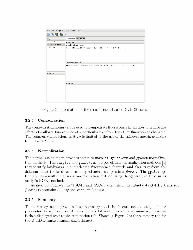
Figure 7: Information of the transformed dataset, GvHD3 trans.

3.2.3 Compensation

The compensation menu can be used to compensate fluorescence intensities to reduce theeffects of spillover fluorescence of a particular dye from the other fluorescence channels.The compensation options in iFlow is limited to the use of the spillover matrix availablefrom the FCS file.

3.2.4 Normalization

The normalization menu provides access to warpSet, gaussNorm and gpaSet normaliza-tion methods. The warpSet and gaussNorm are per-channel normalization methods [1]that identify landmarks in the selected fluorescence channels and then transform thedata such that the landmarks are aligned across samples in a flowSet . The gpaSet op-tion applies a multidimensional normalization method using the generalized Procrustesanalysis (GPA) method.

As shown in Figure 9, the ”FSC-H”and ”SSC-H”channels of the subset data GvHD3 trans subflowSet is normalized using the warpSet function.

3.2.5 Summary

The summary menu provides basic summary statistics (mean, median etc.) of flowparameters for each sample. A new summary tab with the calculated summary measuresis then displayed next to the Annotation tab. Shown in Figure 9 is the summary tab forthe GvHD3 trans sub normalized dataset.

8

Figure 8: Subset data.

Figure 9: Summary tab for the GvHD3 trans sub normalized dataset.

9

3.3 Graphics Menu

Figure 10: Stack Density Plot GUI

The Graphics menu provides several methods to visualize flow cytometry data. Thechoices are:

Contour Plot Opens a new GUI which allows the user to select one or more datasamples and flow channels for X- and Y-axis. Clicking on OK will create contourplots for the currently selected samples.

ECDF Plot Opens a new GUI which allows the user to select one or more samples anda flow channel for X-axis. Clicking on OK will create empirical CDF plots for theselected samples with selected channels.

Dot Plot Opens a new GUI which allows the user to select one or more samples andflow channels for X- and Y-axis. Clicking on will create non-smooth scatter plots.

Histogram Plot Opens a new GUI which allows the user to select a sample and a flowchannel. Clicking on OK will create a frequency plot.

Parallel Coordinates Plot Opens a new GUI which allows the user to select a sampleand a couple or more channels. Clicking on OK will create a parallel coordinateplots.

Q-Q Plot Opens a new GUI which allows the user to select one or more samples anda flow channel. Clicking on OK will creates a quantile plot.

10

Scatter Plot Matrix Opens a new GUI which allows the user to select one sampleand one ore more flow channels. Clicking on OK will create Trellis scatter plotsmatrices (splom) from selected samples.

Smooth Scatter Plot Opens a new GUI which allows the user to select one or moresamples and flow channels for X- and Y-axis. Clicking on OK will create Trellisscatter plots for selected samples.

Stack Density Opens a new GUI which allows the user to select one ore more samplesand flow channels. Clicking on OK will creates horizontal stack plots of densityestimates for selected samples.

Timeline Opens a new GUI which allows the user to select one or more flowFrame(s)and one channel. Clicking on OK will plot values for the selected samples againsta time domain in the dataset. It helps to identify problems related to instrumentsetting when the measurement runs.

workflow Creates a flow chart of the current workflow.

Figure 11: Stack Density Plots.

Continuing the example, we activate ”GvHD3 trans sub normalization” by clickingthe data on Data tab in the control panel. Then, select Graphics|Stack Density Plots.

11

We select all the samples and three channels such as ”FSC-H”, ”SSC-H”, and ”FL1-H” inthe currently activated dataset. The new GUI calling up by Stack Density Plot selectionis shown in Figure 10. Depicted in Figure 11 is the resulting density plot. Note that anycreated plots can be saved in the form of ’png’ file.

12

Figure 12: Workflow plot.

13

Figure 13: Description of a selected object on Gate View

3.4 Gate Menu

The Gate menu contains two options: Create and Combine. The Create option allowsthe user to create gate objects either by manual gating or by the provided auto-gatingmethods. The Combine option allows to combine gate objects.

3.4.1 Create Gates

The Create option provides five selections of auto-geometric gates:

Rectangle Gate Opens new GUIs which allow the user to select two channels for X-and Y-axis and to specify the boundary of the rectangle gate. It than creates aRectangleGate object.

Quadrant Gate Opens a new GUI which allows the user to select channels for X- andY-Axis. It then creates a QuadrantGate object and tries to find the most likelyseparation of the two-dimensional data in four quadrant.

Lymphocyte Gate Opens a new GUI which allows the user to select two channels forX- and Y-axis and specify one or more rough preselection channels. It then createsa LymphFilter object to identify cell population of roughly elliptical shape.

Kmeans Opens a new GUI which allows the user to select one channel. It creates aKmeansFilter object to identify cell population based on one-dimensional k-meansclustering operation.

14

Norm2 Gate Opens a new GUI which allows the user to select two channels for X-and Y-axis. It creates a Norm2Filter object to find a region to mostly resemble abivariate Normal distribution.

Curv1 Gate Opens a new GUI which allows the user to select one channel. It createsa Curv1Filter object to select one-dimensional high-density regions.

Curv2 Gate Opens a new GUI which allows the user to select two channels for X- andY-axis. It creates a Curv2Filter object to select two-dimensional high-densityregions.

For the example, we first create three gate objects. The list of gate objects will beshown on the Gate List tab on the control panel. Additionally, Gate List tab supportssummary and a scatter plot of an object in the activated data by right mouse click onthe panel. The summary tab on the object is generated on the information panel. GateView tab provides description of a selected object. See Figure 13.

3.4.2 Applying Gate Objects

After the Gate objects are created, iFlow allows the user to apply gate objects to thedatasets in the following two ways:

Figure 14: A pup-up GUI for selecting a gate for a subset.

Data|Subset By|Gate Select Data menu and sequentially select Subset By and thenGate items. A new GUI will be created, as shown in Figure 14, allowing the userto select the Gate objects to be applied to the activated dataset.

15

Drag and Drop Drag a gate object on the Gate List panel and drop it onto the dataseton the Data panel.

As illustrated in Figure 15, the ”GvHD3 trans sub” data is filtered by using withNorm2Filter. Consequently, the filtered datasets, ”GvHD3 trans sub gatedefaultNormFilter+”and ”GvHD3 trans sub gatedefaultNormFilter-”, are included in the Data tab as childnodes of activated dataset. Figure 16 displays a dot plot for the ”GvHD3 trans sub gatedefaultNormFilter+”data object.

Figure 15: Filtered data.

3.4.3 Manual Gate

iFlow also supports manual gating to identify cell populations on one or two dimensionalplots. The user can follow the following two simple steps to create a gate object:

1. Select Gate|Create|Manual Gate menu item. A new GUI will appear on the screenallowing the user to choose a sample and flow parameters of interest. A smoothscatter plot will then be created.

2. Draw an enclosed area on the plot by clicking a mouse button on the region ofinterest, as illustrated in Figure 17. When finished, double-click the right mousebutton outside of the plot in the graphics window.

16

Figure 16: Dot plot for the filtered data.

3.4.4 Combine Gates

The Combine Gates option allows the user to combine created gates through one ormore boolean operations such as &, | and !. Upon selecting this option, a new GUI willappear on the screen, as depicted in Figure 18, allowing the user to select the existinggates and the boolean operation. The combined gate object will be created and listedon the Gate List panel as a new gate object.

3.4.5 Backgating

Backgating analysis provides visualization with the gated polulation at each level in agating hierarchy. So it is able to validate gating positions through the display. Theright-most plot on the graphic window shows final gated polulation of events overlaidin a gating hierachy. The summary of the gated population at each level is provided bygenerating summary tab on information panel in the order.

To perform backgating analysis, choose Gate|Backgating menu item, and select gateobjects in order for shown gate objects on gate list panel by clicking on Add. It is alsoable to delete the selected gates on hierarchy panel (of a selected gate list) by clickingon Remove.

For the example, we apply Norm2Filter object to the active data set, then applyNorm2Filter1 object to the gated population through Norm2Filter1. To validate the

17

Figure 17: Drawing an interesting region to create a gate object.

Figure 18: Combine gates

18

Figure 19: GUI for backgating analysis

position of gates, we are able to use backgating function on menu. Figure 19 shows theGUI of Gate|Backgating menu item, users are able to specify the order of gates theywant to apply gate objects to the data. So Figure 20 shows the final gated polulationoverlaid at each level. Therefore, we can easily see whether of not one of selected gatesis correctly applied.

3.5 Help Menu

The Help menu has two options: Manual and iflow.history. The Manual option providesa basic user’s guide for using iFlow. The iFlow.history option is meant to show thehistory of actions (R commands) of the current workflow. Still under development, itnow only works for graphics commands. See Figure 21 for an example.

4 Conclusion

The iFlow package contains all the code necessary to create and run the GUI, but itdoes not contain any code for the analysis of FCS data. Rather, it relies on functionalityimplemented in other R packages such as flowCore, flowStats, and flowViz. It currentlyprovides access to data visualization, manual and automated gating, transformationsand basic data manipulations. This is sufficient for initial exploratory data inspection,as well as for prototyping large analysis projects.

Some of the capabilities exposed by the iFlow, such as automated gating, already gobeyond what is available in standard FCM GUI software. However, the primary long-term advantage of our software is its open and extensible nature. Additional functionality

19

Figure 20: backgating display for the gated population of events overlaid in a gatinghierarchy.

Figure 21: The history of graphics commands for the current workflow.

20

may easily be added in response to user feedback, or once common use cases haveemerged.

21

References

[1] F. Hahne, A. H. Khodabakhshi, A. Bashashati, C.-J. Wong, R. D. Gascoyne, A. P.Weng, V. Seyfert-Margolis, K. Bourcier, A. Asare, T. Lumley, R. Gentleman, andR. R. Brinkman. Per-channel basis normalization methods for flow cytometry data.Cytometry Part A, 77A(2):121–131, 2009.

[2] M. Lawrence and D. Temple Lang. RGtk2: R bindings for Gtk 2.8.0 and above. URLhttp://www.ggobi.org/rgtk2. R package version 2.12.9.

[3] K. Lee, F. Hahne, D. Sarkar, and R. Gentleman. iflow: A graphical user interfacefor flow cytometry tools in bioconductor. Advances in Bioinformatics, 2009, 2009.

[4] The GTK+ Team. http://www.gtk.org/, 2009.

22