How to Excel with CUFS Part 2 (Excel 2010)

How to Excel with CUFS Part 2 Excel 2010

Course Manual Finance Training

Excel version 2010

How to Excel with CUFS Part 2 vs 0.1

Contents

1. Working with multiple worksheets 1.1 Inserting new worksheets 3 1.2 Deleting sheets 3 1.3 Moving and copying Excel worksheets 4 1.4 Adding headers and footers 4 1.5 Changing a worksheet tab colour 5

2. Lookup Tables

2.1 What are they? 7 2.2 Creating a lookup table 7 2.3 Using the lookup formula (VLOOKUP) 8

3. Relative and Absolute references

3.1 Relative references 10 3.2 Absolute references 10 3.3 Ranges of cells 11

4 The SUMIF function 4.1 Using the function wizard with the SUMIF function 13 5. Pivot Tables 5.1 What are PivotTables? 16 5.2 How to create Pivot Tables 17 5.3 The Pivot Table Tool Bar 20 5.4 Changing the level of data displayed 20 5.5 Drilling down to see what a value consist of 21 5.6 changing the fields displayed on the pivot table report 21 5.7 Re-arranging the data displayed 22

How to Excel with CUFS Part 2 vs 0.1 3

1. Working with multiple worksheets and work books

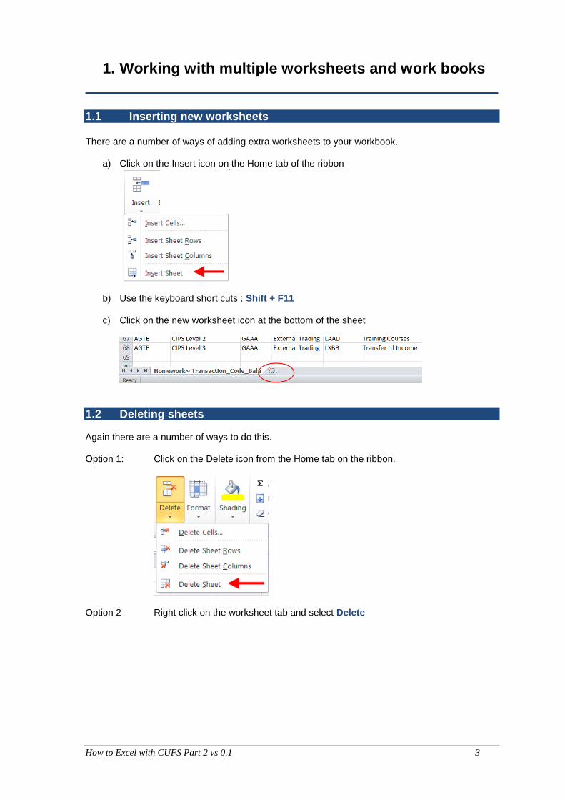
1.1 Inserting new worksheets There are a number of ways of adding extra worksheets to your workbook.

a) Click on the Insert icon on the Home tab of the ribbon

b) Use the keyboard short cuts : Shift + F11

c) Click on the new worksheet icon at the bottom of the sheet

1.2 Deleting sheets

Again there are a number of ways to do this. Option 1: Click on the Delete icon from the Home tab on the ribbon.

Option 2 Right click on the worksheet tab and select Delete

Excel version 2010

How to Excel with CUFS Part 2 vs 0.1 vs0.1 4

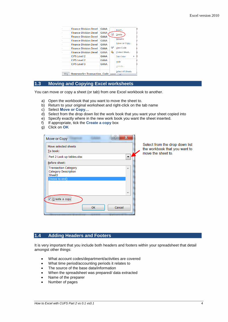
1.3 Moving and Copying Excel worksheets

You can move or copy a sheet (or tab) from one Excel workbook to another.

a) Open the workbook that you want to move the sheet to. b) Return to your original worksheet and right-click on the tab name c) Select Move or Copy… d) Select from the drop down list the work book that you want your sheet copied into e) Specify exactly where in the new work book you want the sheet inserted. f) If appropriate, tick the Create a copy box g) Click on OK

1.4 Adding Headers and Footers It is very important that you include both headers and footers within your spreadsheet that detail amongst other things:

What account codes/department/activities are covered

What time period/accounting periods it relates to

The source of the base data/information

When the spreadsheet was prepared/ data extracted

Name of the preparer

Number of pages

Excel version 2010


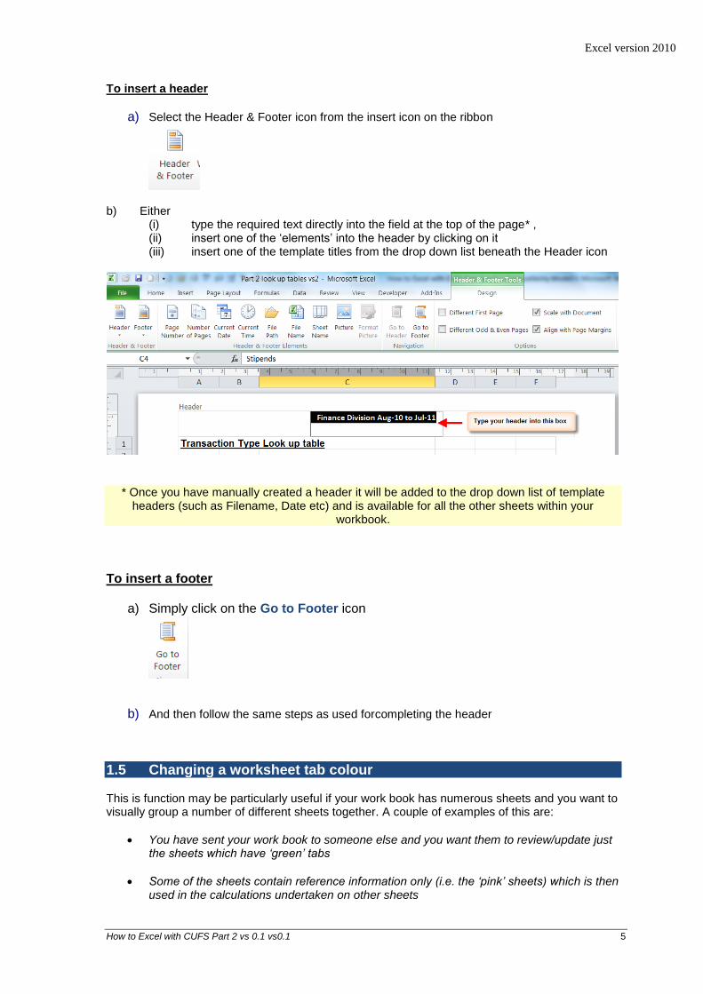
To insert a header

a) Select the Header & Footer icon from the insert icon on the ribbon

b) Either (i) type the required text directly into the field at the top of the page* , (ii) insert one of the ‘elements’ into the header by clicking on it (iii) insert one of the template titles from the drop down list beneath the Header icon

* Once you have manually created a header it will be added to the drop down list of template headers (such as Filename, Date etc) and is available for all the other sheets within your

workbook.

To insert a footer

a) Simply click on the Go to Footer icon

b) And then follow the same steps as used forcompleting the header

1.5 Changing a worksheet tab colour This is function may be particularly useful if your work book has numerous sheets and you want to visually group a number of different sheets together. A couple of examples of this are:

You have sent your work book to someone else and you want them to review/update just the sheets which have ‘green’ tabs

Some of the sheets contain reference information only (i.e. the ‘pink’ sheets) which is then used in the calculations undertaken on other sheets

Excel version 2010


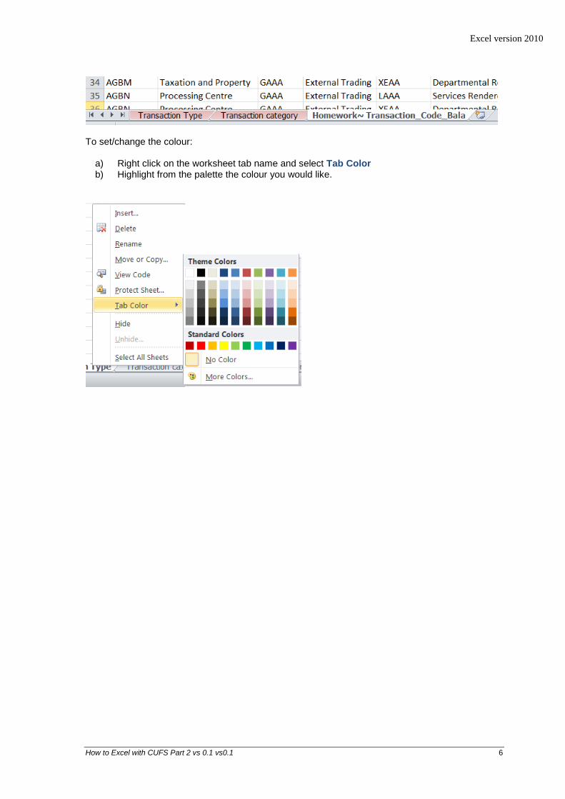
To set/change the colour:

a) Right click on the worksheet tab name and select Tab Color b) Highlight from the palette the colour you would like.

Excel version 2010


2. Lookup Tables

2.1 What are they?

It is sometimes helpful to categorise items in a way that is meaningful to the department but not available in the standard CUFS output. e.g.

Certain cost centres may be grouped together to form a particular division in a department;

Transaction codes can be classified into generic sets (income, expenditure and balance sheet).

You may have a separate spreadsheet holding local departmental budgets for particular cost centres.

So, by assigning department defined categories to a collection of transactions, it is possible to turn CUFS data into tailored information in Excel. For example, in CUFS, all transaction codes beginning with A??? relate to expenditure on stipends and all codes beginning with E??? relate to consumables expenditure. So if a table is set up in Excel (such as the example below), it can then be referenced within a block of data, using a LOOKUP formula to add non-CUFS information to your spreadsheet.

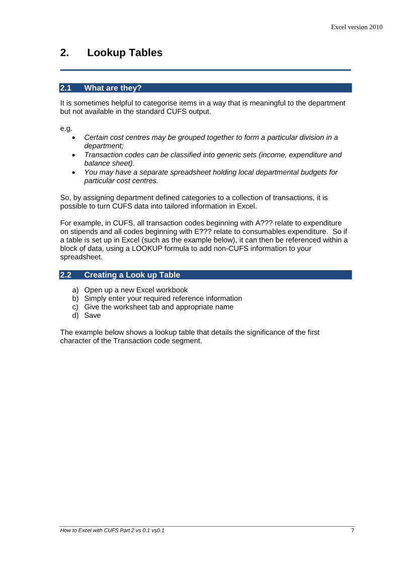
2.2 Creating a Look up Table

a) Open up a new Excel workbook b) Simply enter your required reference information c) Give the worksheet tab and appropriate name d) Save

The example below shows a lookup table that details the significance of the first character of the Transaction code segment.

Excel version 2010


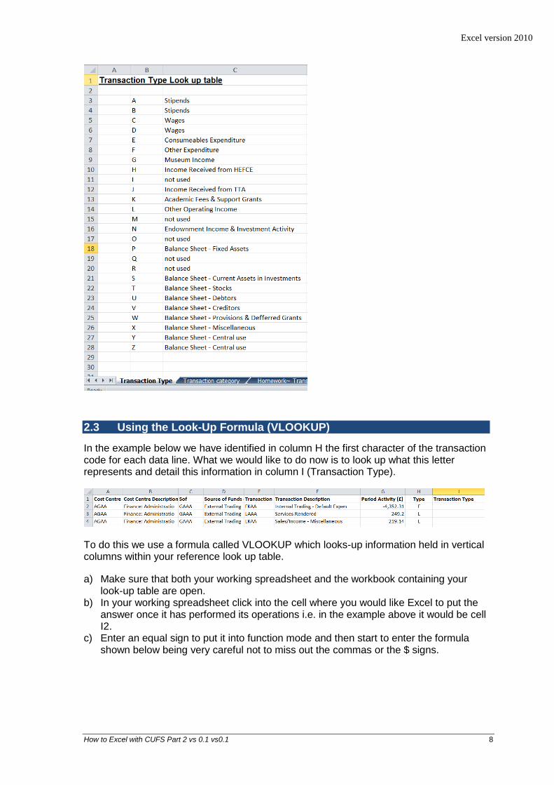
2.3 Using the Look-Up Formula (VLOOKUP)

In the example below we have identified in column H the first character of the transaction code for each data line. What we would like to do now is to look up what this letter represents and detail this information in column I (Transaction Type).

To do this we use a formula called VLOOKUP which looks-up information held in vertical columns within your reference look up table.

a) Make sure that both your working spreadsheet and the workbook containing your look-up table are open.

b) In your working spreadsheet click into the cell where you would like Excel to put the answer once it has performed its operations i.e. in the example above it would be cell I2.

c) Enter an equal sign to put it into function mode and then start to enter the formula shown below being very careful not to miss out the commas or the $ signs.

Excel version 2010


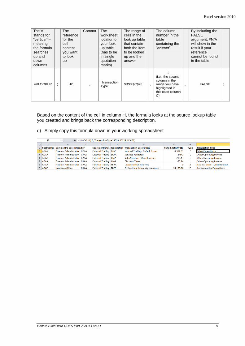
The V stands for “vertical” – meaning the formula searches up and down columns

The reference for the cell content you want to look up

Comma The worksheet location of your look up table (has to be in single quotation marks)

The range of cells in the look up table that contain both the item to be looked up and the answer

The column number in the table containing the “answer”

By including the FALSE argument, #N/A will show in the result if your reference cannot be found in the table

=VLOOKUP

( H2 ,

‘Transaction Type’

$B$3:$C$28 ,

2

(i.e. the second column in the range you have highlighted in this case column C)

, FALSE )

Based on the content of the cell in column H, the formula looks at the source lookup table you created and brings back the corresponding description. d) Simply copy this formula down in your working spreadsheet

Excel version 2010


3 Relative and Absolute cell references

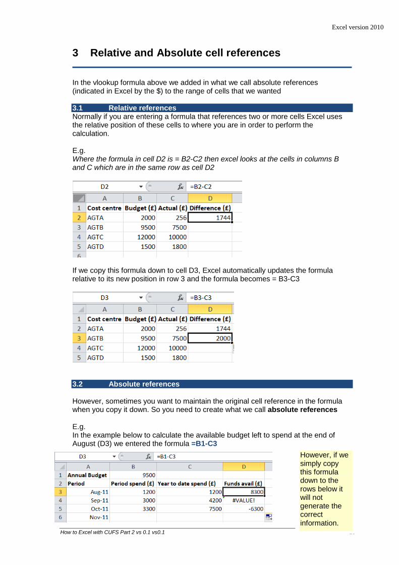
In the vlookup formula above we added in what we call absolute references (indicated in Excel by the $) to the range of cells that we wanted 3.1 Relative references Normally if you are entering a formula that references two or more cells Excel uses the relative position of these cells to where you are in order to perform the calculation. E.g. Where the formula in cell D2 is = B2-C2 then excel looks at the cells in columns B and C which are in the same row as cell D2

If we copy this formula down to cell D3, Excel automatically updates the formula relative to its new position in row 3 and the formula becomes = B3-C3

3.2 Absolute references However, sometimes you want to maintain the original cell reference in the formula when you copy it down. So you need to create what we call absolute references E.g. In the example below to calculate the available budget left to spend at the end of August (D3) we entered the formula =B1-C3

However, if we simply copy this formula down to the rows below it will not generate the correct information.

Excel version 2010


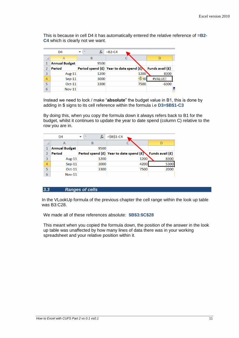
This is because in cell D4 it has automatically entered the relative reference of =B2-C4 which is clearly not we want.

Instead we need to lock / make “absolute” the budget value in B1, this is done by adding in $ signs to its cell reference within the formula i.e D3=$B$1-C3 By doing this, when you copy the formula down it always refers back to B1 for the budget, whilst it continues to update the year to date spend (column C) relative to the row you are in.

3.3 Ranges of cells

In the VLookUp formula of the previous chapter the cell range within the look up table was B3:C28.

We made all of these references absolute: $B$3:$C$28

This meant when you copied the formula down, the position of the answer in the look up table was unaffected by how many lines of data there was in your working spreadsheet and your relative position within it.

Excel version 2010


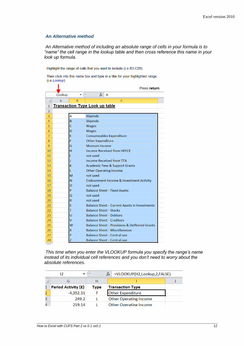
An Alternative method An Alternative method of including an absolute range of cells in your formula is to “name” the cell range in the lookup table and then cross reference this name in your look up formula.

This time when you enter the VLOOKUP formula you specify the range’s name instead of its individual cell references and you don’t need to worry about the absolute references.

Excel version 2010


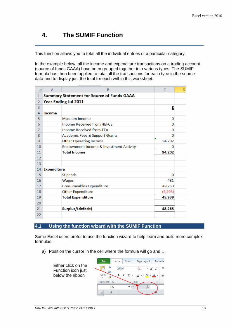
4. The SUMIF Function

This function allows you to total all the individual entries of a particular category. In the example below, all the income and expenditure transactions on a trading account (source of funds GAAA) have been grouped together into various types. The SUMIF formula has then been applied to total all the transactions for each type in the source data and to display just the total for each within this worksheet.

4.1 Using the function wizard with the SUMIF Function Some Excel users prefer to use the function wizard to help learn and build more complex formulas.

a) Position the cursor in the cell where the formula will go and …

Either click on the Function icon just below the ribbon

Excel version 2010


Or select Insert function from the Formulas tab on the ribbon itself.

The Insert Function window appears.

b) In this window you can either type in a search - based on what you are trying to do or select a function from the lists. In this example we want to add a number of cells together, so, when you type “add cells” into the search box, Excel offers a selection of functions.

c) The next part of the wizard invites you to select the cells (or ranges of cells) that contain:

Range The column in the source data that contains the names of the

Items you want it to total e.g. transaction types

Criteria From the summary report the name of the particular transaction type you want it to look for e.g. Other Operating Income

Sum range The column in the source data that contains the values you want it to add together for whichever criteria you have selected.

Select SUMIF from the list and

press OK

Excel version 2010


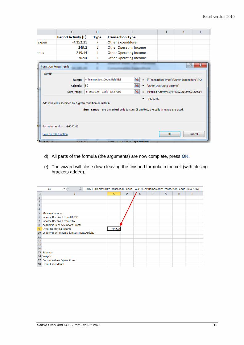
d) All parts of the formula (the arguments) are now complete, press OK.

e) The wizard will close down leaving the finished formula in the cell (with closing brackets added).

Excel version 2010


5. Pivot Tables

5.1 What are pivot tables? Pivot tables are interactive tables in Excel that can quickly summarise or cross-tabulate large amounts of data. They allow you to:

rotate rows and columns to see different layouts of the source data

filter data and display with subtotals and show on different pages

expand the pivot table to see details of one or more items

drill down to create separate detailed data extracts

create charts based on the data with a single click of the mouse Pivot tables also allow you to specify how you would like the data summarised by using functions such as ‘count’, ‘sum’ and ‘average’. Subtotals and grand totals can be included automatically or you can define your own.

You can create a pivot table from:

A Microsoft Excel list or database

Multiple Excel worksheets

An external database

Another pivot table

The Scenario In Excel, analyse departmental expenditure on source of funds AAAA (Chest Non-payroll) by exporting a standard report and creating a pivot table from the data. Method:

Stage 1

Run the Transaction Code Balance Report -Exportable

Save as a Text file and open up in Word to remove page breaks

Import into Excel and save Stage 2

Create a look up table that provides descriptions for the first two letters of the transaction codes starting with E and F

Insert three extra columns into the data spreadsheet and strip out the transaction code details

Using the left function extract the first two characters of the transaction code and look up their description

Stage 3

Select the whole sheet and go to Pivot Reports

Create a pivot report where page = cost centre, rows = category description and data = sum of period activity

Excel version 2010


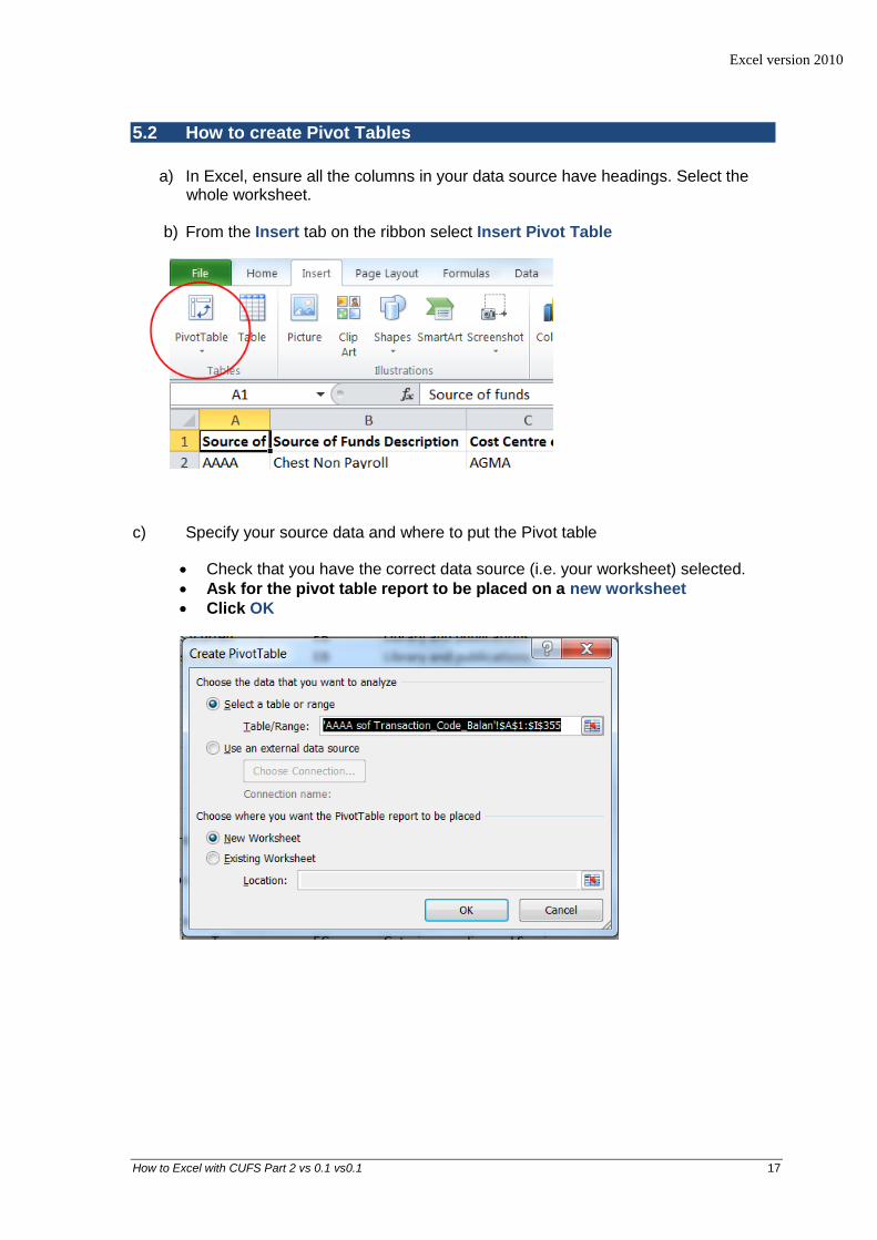
5.2 How to create Pivot Tables

a) In Excel, ensure all the columns in your data source have headings. Select the whole worksheet.

b) From the Insert tab on the ribbon select Insert Pivot Table

c) Specify your source data and where to put the Pivot table

Check that you have the correct data source (i.e. your worksheet) selected.

Ask for the pivot table report to be placed on a new worksheet

Click OK

Excel version 2010


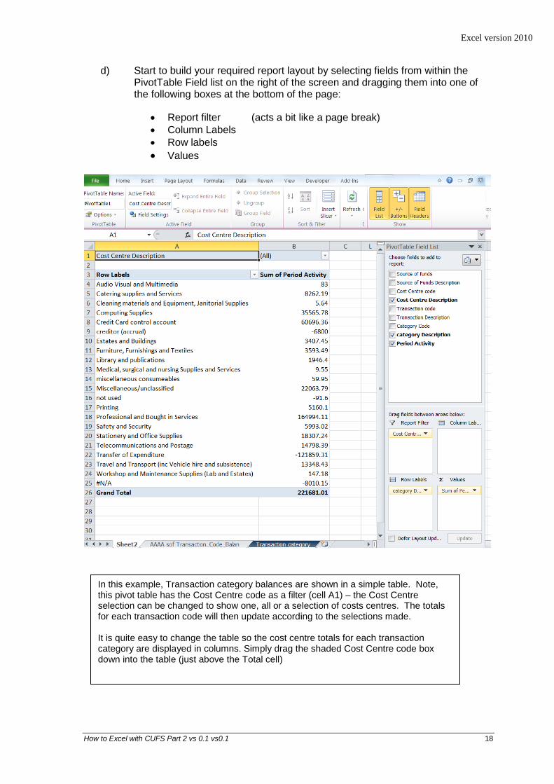
d) Start to build your required report layout by selecting fields from within the PivotTable Field list on the right of the screen and dragging them into one of the following boxes at the bottom of the page:

Report filter (acts a bit like a page break)

Column Labels

Row labels

Values

In this example, Transaction category balances are shown in a simple table. Note, this pivot table has the Cost Centre code as a filter (cell A1) – the Cost Centre selection can be changed to show one, all or a selection of costs centres. The totals for each transaction code will then update according to the selections made. It is quite easy to change the table so the cost centre totals for each transaction category are displayed in columns. Simply drag the shaded Cost Centre code box down into the table (just above the Total cell)

Excel version 2010


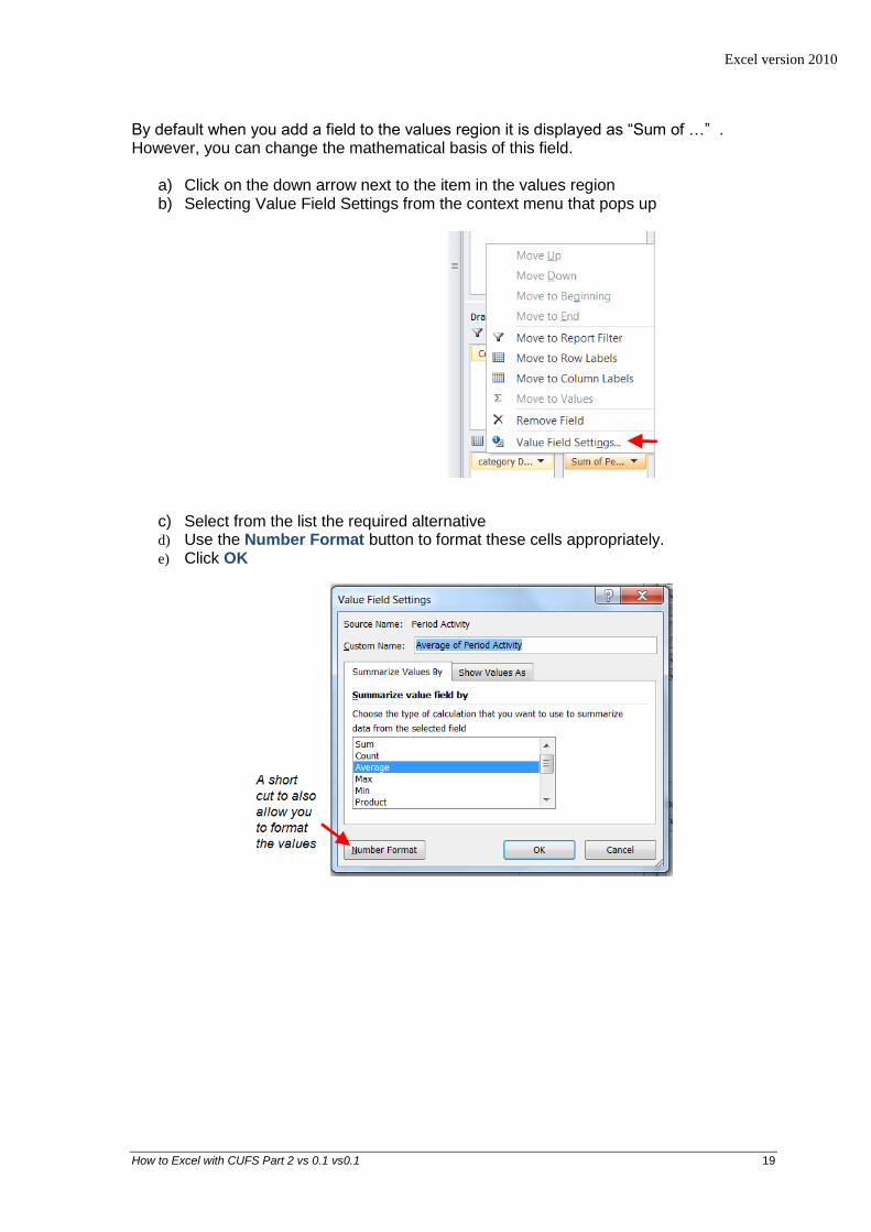
By default when you add a field to the values region it is displayed as “Sum of …” . However, you can change the mathematical basis of this field.

a) Click on the down arrow next to the item in the values region b) Selecting Value Field Settings from the context menu that pops up

c) Select from the list the required alternative d) Use the Number Format button to format these cells appropriately. e) Click OK

Excel version 2010


5.3 The Pivot Table Tool Bar

Make sure that your curser is somewhere within your PivotTable and then above your ribbon a new tab entitled PivotTable Tools should be displayed.

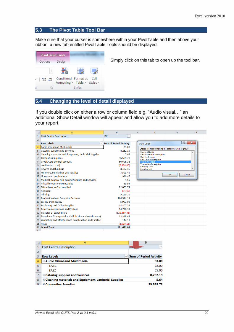
5.4 Changing the level of detail displayed If you double click on either a row or column field e.g. “Audio visual…” an additional Show Detail window will appear and allow you to add more details to your report.

Simply click on this tab to open up the tool bar.

Excel version 2010


5.5 Drilling down to see what a value consists of

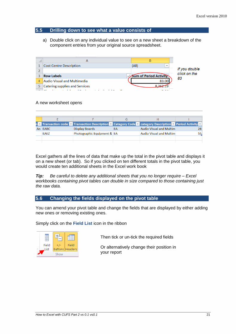
a) Double click on any individual value to see on a new sheet a breakdown of the component entries from your original source spreadsheet.

A new worksheet opens

Excel gathers all the lines of data that make up the total in the pivot table and displays it on a new sheet (or tab). So if you clicked on ten different totals in the pivot table, you would create ten additional sheets in the Excel work book

Tip: Be careful to delete any additional sheets that you no longer require – Excel workbooks containing pivot tables can double in size compared to those containing just the raw data.

5.6 Changing the fields displayed on the pivot table

You can amend your pivot table and change the fields that are displayed by either adding new ones or removing existing ones.

Simply click on the Field List icon in the ribbon

Then tick or un-tick the required fields Or alternatively change their position in your report

Excel version 2010


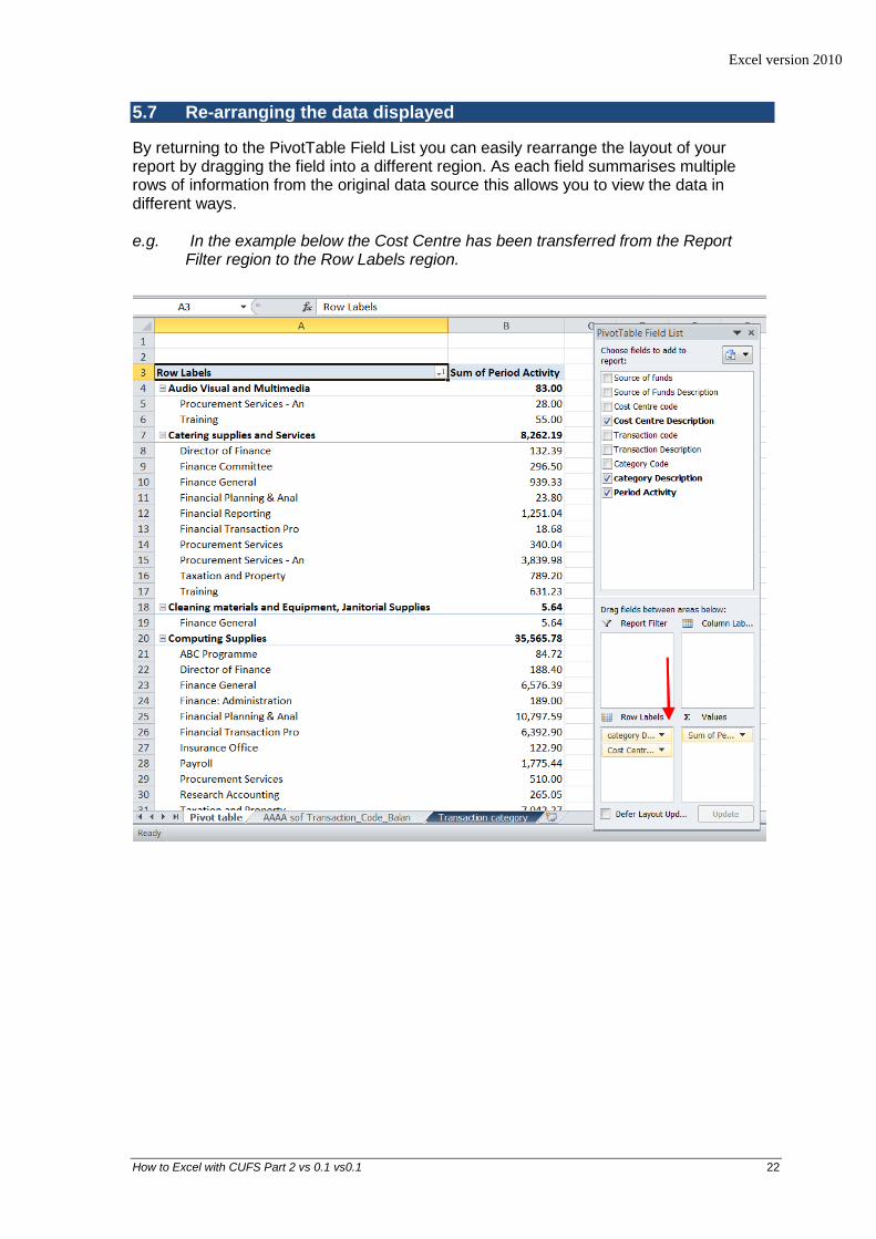
5.7 Re-arranging the data displayed

By returning to the PivotTable Field List you can easily rearrange the layout of your report by dragging the field into a different region. As each field summarises multiple rows of information from the original data source this allows you to view the data in different ways.

e.g. In the example below the Cost Centre has been transferred from the Report

Filter region to the Row Labels region.

Excel version 2010


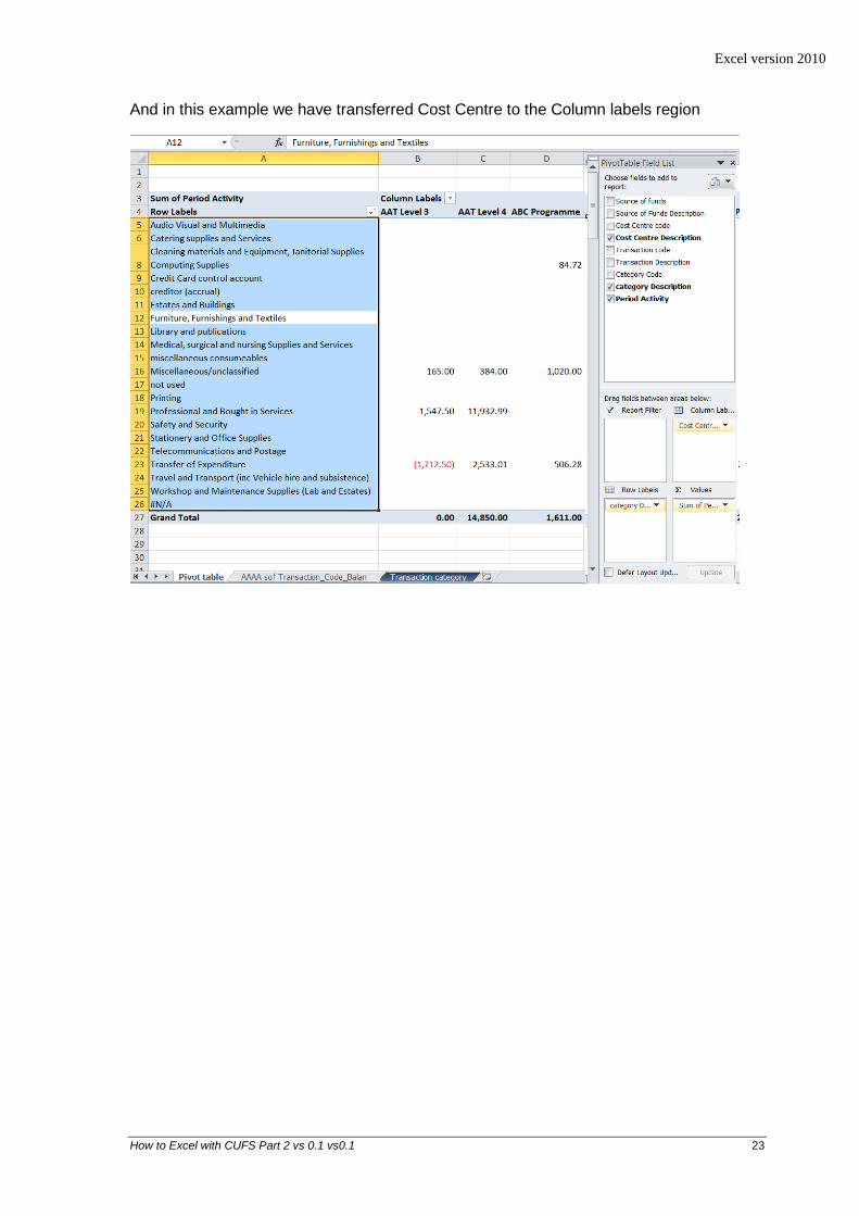
And in this example we have transferred Cost Centre to the Column labels region

Documents

How to Excel with CUFS Part 2 (Excel 2010)