How to Calculate with Shapes

by

George Stiny MIT

‘An interesting question for a theory of semantic information is whether there is any equivalent for the engineer’s concept of noise. For example, if a statement can have more than one interpretation and if one meaning is understood by the hearer and another is intended by the speaker, then there is a kind of semantic noise in the communication even though the physical signals might have been transmitted perfectly.’ — George A. Miller

What to do about ambiguity

It’s really easy to misunderstand when there’s so much noise. Shapes are simply filled with ambiguities. They don’t have definite parts. I can divide them anyhow I like anytime I want. The shape

includes two squares

four triangles

and indefinitely many K’s like the ones I have on my computer screen right now. There are upper case K’s

����� ����� �����

lower case k’s

1

���������������

and their rotations and reflections. These are fixed in the symmetry group of the shape. All of its parts can be flipped and turned in eight ways

And I can divide the shape in myriad myriads of other ways. I can always see something new. Nothing stops me from changing my mind and doing whatever seems expedient. These additional parts

scarcely begin to show how easy it is to switch from division to division without rhyme or reason. (The fantastic number ‘myriad myriads’ is one of Coleridge’s poetic inventions. It turns a noun into an adjective. It’s another example of the uncanny knack of artists and madmen to see triangles and K’s after they draw squares. I do the trick every time I apply a rule to a shape in a computation. There’s no magic in this. I can show exactly how it works. But maybe I am looking too far ahead. I still have a question to answer.)

What can I do about ambiguity? It causes misunderstanding, confusion, incoherence, and scandal. Adversaries rarely settle their disputes before they define their terms. And scientific progress depends on accurate and coherent definitions. But it’s futile trying to remove ambiguity completely with necessary facts, authoritative standards, or common sense. Ambiguity isn’t something to remove. Ambiguity is something to use. The novelty it brings makes creative design possible. The opportunities go on and on. There’s no noise, only the steady hum of invention.

In this chapter, I use rules to calculate with shapes that are ambiguous. This is important for design. I don’t want to postpone computation until I have figured out what parts there are and what primitives to use — this happens in

2

heuristic search, evolutionary algorithms, and optimization. Design is more than sorting through combinations of parts that come from prior analysis (how is this done?), or evaluating schemas in which divisions are already in place. I don’t have to know what shapes are, or to describe them in terms of definite units — atoms, components, constituents, primitives, simples, and so on — for them to work for me. In fact, units mostly get in the way. How I calculate tells me what parts there are. They’re evanescent. They change as rules are tried.

How to make shapes without definite parts

At the very least, shapes are made up of basic elements of a single kind: either points, lines, planes, or solids. I assume that these can be described with the linear relationships of coordinate geometry. My repertoire of basic elements is easily extended to include curves and exotic surfaces, especially when these are described analytically. But the results are pretty much the same whether or not I allow more kinds of basic elements. So I’ll stay with the few that show what I need to. A little later on, I say why I think straight lines alone are enough to see how shapes work.

Some of the key properties of basic elements are summarized in Table 1. Points have no divisions. But lines, planes, and solids can be cut into discrete pieces — smaller line segments, triangles, and tetrahedrons — so that any two are connected in a series of pieces in which successive ones share a point, an edge, or a face. More generally, every basic element of dimension greater than zero has a distinct basic element of the same dimension embedded in it, and a boundary of other basic elements that have dimension one less.

____________________________________________________________

Table 1

Properties of Basic Elements

Basic element Dimension Boundary Content Embedding

point 0 none none identity

line 1 two points length partial order

plane 2 three or more area partial order lines

solid 3 four or more volume partial order planes

____________________________________________________________

3

Shapes are formed when basic elements of a given kind are combined, and their properties follow once the embedding relation is extended to define their parts.

There are conspicuous differences between shapes made up of points and shapes containing lines, planes, or solids. First, shapes with points can be made in just one way if the order in which points are located doesn’t matter, and in only finitely many ways even if it does. Distinct shapes result when different points are combined. But there are indefinitely many ways to make shapes of other kinds. Distinct shapes need not result from different combinations of lines, planes, or solids when these basic elements fuse.

The shape

can be made with eight lines

as a pair of squares with four sides apiece, with twelve lines

as four triangles with three sides apiece, or with 16 lines as two squares and four triangles. But there’s something very odd about this. If the 16 lines exist independently as units that neither fuse nor divide in combination — if they’re like points — then the outside square is visually intact when the squares or the triangles are erased. I thought the shape would disappear. And that’s not all. The shape looks the same whether the outside square is there or not. There are simply too many lines. Yet they make less than I see. I can find only four upper case K’s, and no lower case k’s. Lines are not units, and neither are other basic elements that are not points.

Of course, shapes are ambiguous when they contain points and when they don’t. They can be seen in different ways depending on the parts I actually resolve (or as I show below, on how I apply rules to calculate). But the potential material for seeing is not the same for shapes with points and for shapes made with other basic elements. Points can be grouped to form only a finite number of parts, while shapes of other kinds can be divided into any number of parts in any

4

number of ways. This shape

with three points has just eight possible parts: one empty part, and these seven nonempty ones

� � � � � � �

containing one or more of the points used to make the shape. I can show all of the different ways I am able to see the shape — at least as far as parts go — and count them. But the shape

has indefinitely many parts that need not combine the lines originally used to make it. How the shape is made and how it is divided into parts afterwards are independent. What I find in the shape now may alter later. I can always see something new I haven’t seen before. There is no end to ambiguity and the novelty it brings once basic elements aren’t points.

The contrast between points and basic elements of other kinds that I am beginning to develop leads to alternative models of computation. The first is standard and uncontroversial, but no less speculative for that. The idea simply put is this:

Computation depends on counting.

Points make counting possible. They provide the units to measure the size or complexity of shapes, and the ultimate constituents of meaning. The second model comes from drawing and looking at shapes. The idea is this:

Computation depends on seeing.

Now parts of shapes are artifacts of computations not fixed beforehand. There are neither predefined units of measurement nor final constituents of meaning. Units change freely as I calculate. They may be different every time I apply a rule, even the same rule in the same place.

The contrast can be traced to the embedding relation. For points, it is identity, so that each contains only itself. This is what units require. But for the

5

other basic elements, there are indefinitely many of the same kind embedded in each and every one: lines in lines, planes in planes, and solids in solids. This is a key difference between points and basic elements of other kinds. It implies the properties of the algebras I define for shapes in which basic elements fuse and divide, and lets rules handle ambiguity in computations.

But the contrast is not categorical. These are reciprocal approaches to computation. Each includes the other in its own way. My algebras of shapes begin with the counting model. It’s a special case of the seeing model where the embedding relation and identity coincide. And I can deal with the seeing model in the counting one — and approximate it in computer implementations — using established devices, for example, linear descriptions of basic elements and their boundaries, canonical representations of shapes in terms of maximal elements, and reduction rules. The equivalencies show how complex things made up of units are related to shapes without definite parts.

Whether there are units or not is widely used to distinguish verbal and visual media — discursive and presentational forms of symbolism — as distinct modes of expression. But verbal and visual media may not be as incompatible as this suggests. Shapes made up of points and shapes with lines, planes, or solids belie the idea that there are adverse modes of expression. This makes art and design when they are visual as computational as anything else. The claim is figuratively embedded — if not literally rooted — in the following details.

Algebras of shapes come in a series

Three things go together to define algebras of shapes. First, there are the shapes themselves that are made up of basic elements. Second, there is the part relation on shapes that includes the Boolean operations. And third, there are the Euclidean transformations. The algebras are enumerated up to three dimensions in this series

U0 0 U0 1 U0 2 U0 3

U1 1 U1 2 U1 3

U2 2 U2 3

U3 3

The series is presented as an array to organize the algebras with respect to a pair of numerical indices. (The series goes on in higher dimensions, and not without practical gain. The possibilities are worth thinking about.)

6

Every shape in an algebra Ui j is a finite set of basic elements. These are maximal: any two embedded in a common element are discrete, with boundary elements that are, too. The left index i determines the dimension of the basic elements, and the right index j gives the dimension in which they go together and the dimension of the transformations. The part relation compares shapes two at a time — it holds when the basic elements of one are embedded in basic elements of the other — and the Boolean operations combine shapes. Either sum, product, and difference will do, or equivalently, symmetric difference and product. The transformations are operations on shapes that change them into geometrically similar ones. They distribute over the Boolean operations. The transformations also form a group under composition. Its properties are used to describe the behavior of rules.

A few illustrations help to fix the algebras Ui j visually. And in fact, this is just the kind of presentation they are meant to support. Once the algebras are defined, what you see is what you get. There is no need to represent shapes in symbols to calculate with them, or for any other reason. Take the shapes in the algebra U0 2 . This one

is an arrangement of eight points in the plane. It’s the boundary of the shape

in the algebra U1 2 that contains lines in the plane. The eight longest lines of the shape — the lines someone trained in drafting would choose to draw — are the maximal ones. And in turn, the shape is the boundary of the shape

in the algebra U2 2 . The four largest triangles in the shape are maximal planes. They’re a good example of how this works. They’re discrete and their boundary elements are, too, even though they touch. Points aren’t lines, and aren’t in the boundaries of planes.

For every algebra Ui j

than or equal to i. Shapes can be manipulated in any dimension at least as big as the dimension of the basic elements combined to make them.

, i is greater than or equal to zero, and j is greater

7

The properties of basic elements are extended to shapes in Table 2. The index i is varied to reflect the facts in Table 1. The first thing to notice is that an algebra Ui j contains shapes that are boundaries of shapes in the algebra Ui+1 j

only if i and j are different. The algebras Ui i do not include shapes that are boundaries, and they’re the only algebras for which this is so. They also have special properties in terms of embedding and the transformations. These are described a little later on.

____________________________________________________________

Table 2

Some Properties of Shapes

Algebra Basic elements Boundary shapes Number of parts

U0 j points none finite

U1 j lines U0 j infinite

U2 j planes U1 j infinite

U3 j solids U2 j infinite ____________________________________________________________

The description of parts in Table 2 misses some important details. These require the index j. The additional relationships are given in Table 3.

____________________________________________________________

Table 3

More Properties of the Part Relation

Ui j Every shape has a distinct Every shape is a distinct nonempty part: there is no part of another shape: smallest shape there is no largest shape

0 = i = j no no

0 = i < j no yes

0 < i ≤ j yes yes ____________________________________________________________

Boolean divisions

The algebras of shapes Ui j

properties, and in terms of their Euclidean ones. The Boolean classification are usefully classified in terms of their Boolean

8

relies on the variation of the indices i and j in Table 3. The algebras Udivided this way

i j are

���� ���� ���� ����

���� ���� ����

���� ����

����

according to whether or not i and j are zero. There are four regions to examine: the top row and each of its two segments, and the triangular portion of the lower quadrant.

The atomic algebras of shapes are defined when the index i is zero

���� ���� ���� ����

���� ���� ����

���� ����

����

Shapes are finite arrangements of points. The atoms — nonempty shapes without distinct nonempty parts — are the shapes with a single point apiece. (Atoms are the same as the units I’ve been talking about, but with respect to sets of points and the part relation instead of individual points and embedding.) Any product of distinct atoms is the empty shape, and sums of atoms produce all of the other shapes. No two shapes are the same unless their atoms are. A shape is either empty or has an atom as a part. There are two kinds of atomic algebras depending on the value of the index j.

The only Boolean algebra of shapes is U0 0

���� ���� ���� ����

���� ���� ����

���� ����

����

It contains exactly two shapes: the empty shape and an atom made up of a single point. In fact, it is the only finite algebra of shapes, and it is the only complete one in the sense that shapes are defined in all possible sums and products. The algebra is the same as the Boolean algebra for ‘true’ and ‘false’ used to evaluate logical expressions.

9

The other atomic algebras U0 j are defined when j is more than zero

���� ���� ���� ����

���� ���� ����

���� ����

����

Each of these algebras contains infinitely many shapes that all have a finite number of points, and a finite number of parts. But since there are infinitely many points, there is no universal shape that includes all of the others, and so no complements. This defines a generalized Boolean algebra. It’s a relatively complemented, distributive lattice when the operations are sum, product, and difference, or a Boolean ring with symmetric difference and product. There is a zero in the algebra — the empty shape — but no universal element, as this would be a universal shape. As a lattice, the algebra is not complete: every product is always defined, while no infinite sum ever is. Distinct points don’t fuse in sums the way basic elements of other kinds do. The finite subsets of an infinite set, say, the numbers in the counting sequence 0, 1, 2, 3 . . . , define a comparable algebra.

This idea comes up again when I consider algebras for decompositions. A decomposition is a finite set of parts (shapes) that add up to make a shape. It gives the structure of the shape by showing just how it’s divided, and how these divisions interact. The decomposition may have special properties, so that parts are related in some way. It may be a Boolean algebra on its own, a topology, a hierarchy, or even something else. For example, suppose that a singleton part contains a single basic element. These are atoms in the algebras U0 j but don’t work this way if i isn’t zero. The set of singleton parts of a shape with points is a decomposition. In fact, the shape and the decomposition are pretty much alike. But decompositions are not defined for shapes with basic elements of any other kind. There are infinitely many singleton parts.

Algebras of shapes show what happens when shapes are put together using specific operations. But there are complementary accounts that are also useful. Looking at individual shapes in terms of their parts — whether or not these are finite in number — is another way of describing algebras of shapes with subalgebras. Don’t be alarmed as I move to and fro between these views. It’s not unlike seeing shapes in different ways. For starters, a shape and its parts in an algebra U0 j form a complete Boolean algebra that corresponds to the Boolean algebra for a finite set and its subsets. This is represented neatly in a lattice diagram. For example, the Boolean algebra for the three points

10

in U0 2 considered above looks like this

Pictures like this are compelling, and make it tempting to consider all shapes — whether or not they have points — in terms of a finite number of parts combined in sums and products. It’s hard to imagine a better way to describe shapes than to resolve their parts and to show how these are related. This is what decompositions do. But if parts are fixed permanently, then this is a poor way to understand how shapes work in computations. As I describe this below, parts — with and without Boolean complements — vary within computations and from one computation to the next. Parts are decided anew every time I apply a rule. Decompositions — topologies and the like — change dynamically as I go on calculating. I don’t know what parts there really are until I stop.

The Boolean algebra for a shape and its parts in an algebra U0 j is itself a discrete topology. Every part of the shape is both closed and open, and has an empty boundary. Parts are disconnected. (Topological boundaries aren’t the boundaries of Table 2 that show how shapes in different algebras are related. Now the boundary of a shape is part of it.) This is a formal way of saying what seeing confirms all the time: there is no preferred way to divide the shape into parts. Any division is possible. None is better or worse than any other without ad hoc reasons. These depend on how rules are used to calculate.

To return now to the algebras Ui j

more than zero , the atomless ones are defined when i is

���� ���� ���� ����

���� ���� ����

���� ����

����

Each of these algebras contains infinitely many shapes made up of a finite number of lines, planes, or solids. But every nonempty shape has infinitely many parts. The empty shape is the zero in the algebra. There is no universal element — a universal shape can’t be formed with lines, planes, or solids — and shapes don’t have complements. This gives a generalized Boolean algebra, as above

11

for points. But this time, the properties of sums and products are a little more alike: for both, infinite ones may or may not be defined. When infinite sums are formed, basic elements fuse.

In an algebra Ui j when i isn’t zero, a nonempty shape and its parts form an infinite Boolean algebra. But the algebra is not complete. Infinite sums and products needn’t determine shapes. The underlying topology for the shape and its parts is a Stone space. Every part is both closed and open, and the part has an empty boundary. Parts are disconnected. In this, all shapes are exactly the same. They’re all ambiguous. There’s nothing about shapes by themselves — no matter what basic elements they have — that recommends any division. It’s only in computations as a result of what rules do that shapes have definite parts with meaningful interactions, and the possibility of substantial boundaries.

So far, my classification of shapes and their algebras shows that things change significantly once i is bigger than zero. Whether or not the embedding relation implies identity makes a world of difference. But my algebras are not the only way to think about shapes. There are two alternatives that deserve brief notice.

First, there are the individuals of logic and philosophy. Shapes are like them in important ways. The part relation is crucial for both. But the likeness fades once other details are compared. Individuals form a complete Boolean algebra that has the zero excised. The algebra may have atoms or not, and may be finite or infinite. Moreover, there are no ancillary operators. Transformations are not defined for individuals. To be honest, though, the nonempty parts of any nonempty shape in an algebra U0 j are possible individuals. But if j isn’t zero, then this isn’t so for all of the nonempty shapes in the algebra taken together. Individuals are pointless, unless they exercise their right to free assembly finitely.

Second, there are the point sets of solid modeling. But the topology of a shape in an algebra Ui j when i isn’t zero and the topology of the corresponding point set are strikingly different. The shape is disconnected in the one topology and connected in the other. Among other things, the topology of the point set confuses the boundary of the shape that’s not part of it — the boundary of Table 2 — and the topological boundary of the shape that is. Points are too small to distinguish boundaries as limits and parts. Point sets are ‘regular’ whenever they’re shapes, and Boolean operations are ‘regularized’. This is an artificial way to handle lines, planes, and solids. Of course, shapes made up of points are point sets with topologies in which parts are disconnected. This and my description of individuals confirm what I’ve already said. The switch from the identity relation to embedding is modest technically, but has many important consequences for shapes.

12

Euclidean embeddings

The Euclidean transformations augment the Boolean operations in the algebras of shapes U

i j with additional operators. They are defined for basic

elements and extend easily to shapes. Any transformation of the empty shape is the empty shape. And a transformation of a nonempty shape contains the transformation of each of the basic elements in the shape. This relies on the underlying recursion implicit in Tables 1 and 2 in which boundaries of basic elements are transformed until new points are defined.

The universe of all shapes no matter what kind of basic elements are involved can be described as a set containing certain specific shapes, and other shapes formed using the sum operation and the transformations. For points and lines, the universe is defined with the empty shape and a shape that contains a single point or a single line. Points are geometrically similar, and so are lines. But this relationship doesn’t hold for planes and solids. As a result, more shapes are needed to start. All shapes with a single triangle or a single tetrahedron do the trick. For a point in zero dimensions, the identity is the only transformation. So there are exactly two shapes: the empty shape and the point itself. In all other cases, there are indefinitely many distinct shapes that come with any number of basic elements. Every nonempty shape is geometrically similar to indefinitely many other shapes.

The algebras of shapes Ui j also have a Euclidean classification that

refines the Boolean classification given above. Together these classifications form an interlocking taxonomy. The algebras U

i i on the diagonal provide the

main Euclidean division

���� ���� ���� ����

���� ���� ����

���� ����

����

The algebras Ui i have an interesting property. A transformation of every

shape in each algebra is part of every nonempty shape. This is trivially so in the algebra U

0 0

���� ���� ���� ����

���� ���� ����

���� ����

����

13

for a point in zero dimensions. Both the empty shape and the point are parts of the point. But when i is not zero

���� ���� ���� ����

���� ���� ����

���� ����

����

the possibilities multiply. In this case, infinitely many transformations of every shape are parts of every nonempty shape. This is obvious for the empty shape. It’s part of every shape under every transformation. But for a nonempty shape, there is a little more to do. The basic elements in the shape are manipulated in their own dimension: lines are in a line, planes are in the plane, and solids are in space. And since these basic elements are separately finite, finite in number, and finitely arranged, they can always be embedded in a single basic element. But infinitely many transformations of any basic element can be embedded in any other basic element. I can make the one smaller and smaller until it fits in the other and can be moved around. So there are infinitely many ways to make any shape part of any other shape that has at least one basic element. The triangle

in the algebra U2 2 is geometrically similar to parts of a rectangle

and in fact, to parts of itself

This has important implications for the way rules work in computations. As defined below, a rule applies under a transformation that makes one shape part of another shape. Everything is fine if the rule is given in the algebra U0 0 . It’s determinate: if it applies, it does so under a finite number of transformations. And in fact, there are determinate rules in every algebra containing shapes with points. But in the other algebras Ui i , a rule is always indeterminate: it applies to every nonempty shape in infinitely many ways as described above. (There are

14

indeterminate rules for points, too, when j is greater than zero.) This eliminates any chance of controlling how the rule is used. It can be applied haphazardly to change shapes anywhere there is an embedded basic element. Indeterminate rules seem to be a burden. They appear to be totally purposeless when they can be applied so freely. Even so, indeterminate rules have some important uses. A few of these are described below.

I like to think that shapes made up of lines in the plane — a few pencil strokes on a scrap of paper — are all that’s ever required to study shapes and computations with them. There are reasons for this that are both historical and practical. On the one hand, for example, lines are central in Alberti’s famous account of architecture, and on the other hand, the technology of making lines isn’t very complicated. But an algebraic reason supersedes all of the others. Shapes containing lines arranged in the plane suit my interests because their algebra U1 2

���� ���� ���� ����

���� ���� ����

���� ����

����

is the first algebra of shapes in the series Ui j in which (1) basic elements have boundaries and the identity relation and embedding are not the same, and (2) there are rules that are determinate and rules that aren’t — rules in U1 1 are also indeterminate in U1 2 — when I apply them to shapes to calculate. The algebra U1 2 is representative of all of the algebras where i isn’t zero. This lets me show almost everything I want to about these algebras and the shapes they contain in line drawings. Lines on paper are an excellent way to experiment with shapes, and to see how they work in computations.

More algebras in new series

The algebras Ui j can themselves be extended and combined in a host of useful ways to define new algebras of shapes. This provides an open-ended repertoire of shapes and other kinds of expressive devices.

Shapes often come with other things besides basic elements. Labels from a given vocabulary, for example, a, b, c . . . , may be associated with basic elements to get shapes like these

15

� �

� �

� �

�

�

�

The labels may simply classify basic elements and so parts of shapes, or they may have their own semantics to introduce new kinds of information. In a more ambitious fashion, basic elements may also have properties associated with them that interact as basic elements do when they are combined. I call these weights. Weights may go together with basic elements to get shapes like these

Among other things, weights include different graphical properties such as color, surface texture, and tone, but possibly more abstract things like sets of labels, numerical values that vary in some way, or combinations of sets and values. (Weights can also be shapes. This may complicate how shapes are classified, but doesn’t compromise the idea that the embedding relation makes a difference in computation.)

Labels and weights let me show how shapes can go together in different ways. I can put a triangle on top of a square to make the shape

in the algebra U12, and then take away the triangle I’ve added. But the result isn’t the square

that might be expected just listening to the words ‘take away the triangle after adding it to the square’. The piece the triangle and square have in common is erased from the top of the square as happens in drawing. This gives the shape

16

But I have other options. I can label the lines in the triangle in one way and label the lines in the square in another way, so that the square is still intact after adding and subtracting the triangle. Borrowing a term from computer graphics, the triangle and the square are on separate layers. And I can do the same thing and more with weights. Either way, this begins to show how labels and weights can be used to modify algebras of shapes. It also anticipates some properties of decompositions I describe in the next section.

When labels and weights are associated with basic elements, additional algebras of shapes are defined. Two new series of algebras are readily formed from the series Ui j . The algebras Vi j for labeled shapes keep the properties of the algebras Ui j , and the algebras Wi j for weights may or may not, according to how weights combine. For example, notice that if labels are combined in sets, then the series of algebras Wi j includes the series Vi j . Of course, it’s always possible to extend the algebras Ui j in other ways if there’s an incentive. There’s no reason to be parsimonious — and no elegance is lost — when algebras that fit the bill are so easy to define.

The algebras Ui j, Vi j, and Wi j can also be combined in a variety of ways, for example, in appropriate sums and products (direct products), to obtain new algebras. These algebras typically contain compound shapes with one or more components in which basic elements of various kinds, labels, and weights are mixed and interact, as for example, in the shape

�

In this way, the algebras Ui j, Vi j, and Wi j, and their combinations facilitate the definition of a host of formal devices in a uniform framework. The properties of these devices correspond closely to the properties of traditional media in art and design. Nothing is lost — certainly no ambiguity. This lets me calculate in the kind of milieu that’s expected for creative activity, at least as it’s normally understood.

The algebras I’ve been talking about give me the wherewithal to say what I mean by a design. Roughly speaking, designs are used to describe things for making and to show how they work. This may imply a wide range of expressive devices — shapes and the kinds of things in my algebras — in a host of different descriptions that are linked and interact in various ways. Formally then, designs belong to n-ary relations in my algebras. The computational apparatus I’m coming to is meant to define these relations. And in fact, there are already many successful examples of this in architecture and engineering.

17

Solids, fractals, and other zero dimensional things

I said earlier that decompositions are finite sets of parts that sum to make shapes. They show how shapes are divided into parts for different reasons and how these divisions interact. Of course, decompositions are not just defined for shapes in an algebra Ui j . More generally, they’re defined for whatever there is in any algebra formed from the algebras in the series Ui j . And decompositions have their own algebras. Together with the empty set — it’s not a decomposition — they form algebras under the subset relation, the Boolean operations for sets (union, intersection, and so on), and the Euclidean transformations. This makes decompositions zero dimensional. They’re the same as shapes in the algebras U0 j . The parts they contain behave just like points. Whatever else they may be, the parts in decompositions are units. They’re independent in combination and simple beyond analysis.

I like to point out that complex things like fractals and computer models of solids and thought are zero dimensional. Am I obviously mistaken? Solids are clearly three dimensional — I bump into them all of the time — fractal dimensions vary widely, and no one knows for sure about thought. But this misses the point. Fractals and computer models utilize decompositions that are zero dimensional, or other representations such as lists or graphs in which units are likewise given from the start. But what’s wrong with this? Computers are meant to manipulate complex things — fractals and the like — that have predefined divisions. They’re especially good at counting units — fractal dimensions are defined in this way — and moving them around to go through possible configurations. Yet computers fail with shapes once they include lines or basic elements of higher dimension. I can describe what happens to shapes so long as I continue to calculate, and measure their complexity as a result of the rules I apply to pick out parts. In this sense, shapes may be just as complex as anything else. There is, however, a telling difference. The complexity of shapes is retrospective. It’s an artifact of my computation that can’t be defined independently. There aren’t any units to count before I calculate. What can I do about this?

I have already shown that units in combination need not correspond with experience. What a computer knows and what I see may be very different. And the computer has zero tolerance for views that aren’t its own. The shape

as 16 lines that describe two squares with four sides apiece and four triangles with three sides apiece doesn’t behave the way it should. There are too many

18

lines and just too few. For example, some parts are hard to delete. The outside square won’t go away. And some parts are impossible to find. The lower case k’s aren’t there. But even if I’m willing to accept this because the definitions of squares and triangles are exactly what they should be — and for the time being they’re more important than k’s — there’s still a problem. How am I going to find out how the shape is described before I start to use it? Does it include squares or triangles, or is it a combination of both? I can see the shape, but I can’t see its decomposition. It’s inside the computer. I need to find this hidden structure. Experiments are useful, but they take time and may fail. I’m stuck without help and the occult (personal) knowledge of experts. Shapes aren’t like this. What you see is what you get. This is a good reason to use shapes in design. There are times when I don’t know what I’m doing and look at shapes to find out. But there’s nothing to gain if I have to ask somebody what shapes are. Can I make decompositions that are closer to the shapes they describe?

It’s not hard to guess that my answer is going to be no. There are many reasons for this, but a few are enough to support my conclusion. First, there is the problem of the original analysis. How can I possibly know how to divide a shape into parts that suit my present interests and goals — everything is vague before I start to calculate — and that anticipate whatever I might do later? I can change my mind. Nothing keeps me from seeing triangles and K’s after I draw squares, even if I’m positive squares are all I’ll ever need. Contracts aren’t hard to break. It’s so much easier to see what I want to in an ongoing process than to remember or learn what to do. My immediate perception may take precedence over anything I’ve decided or know for sure. But there is an option. I don’t have to divide the shape into meaningful parts. I can cut it into anonymous units that are small enough to model (approximate) as many new parts as I want. This is a standard practice that doesn’t work. The parts of the shape and their models are too far apart. Shapes containing lines, for example, aren’t like shapes that combine points. This is what the algebras U0 j and U1 j

show. Moreover, useful divisions are likely to be infrequent and not very fine. Getting the right ones at the right time is what matters. But even if units do combine to model the parts I want, they may also multiply unnecessary parts well beyond interest and use to cause unexpected problems. Point sets show this perfectly. I have to deal with the parts I want, and the parts I don’t. If I’m clever, this won’t stop me. But there is a price to pay. Dividing the shape into smaller and smaller units may exceed my intuitive reach. I can no longer engage the shape directly in terms of what I see. Now there’s something definite to know beforehand. Expertise intervenes. I have to think twice about how the shape works as a collection of arbitrary units that go together in an arbitrary way. What happens to novelty and the chance of new experience? Anyhow you cut it, there’s got to be a better way to handle the shape. Decompositions are premature before I calculate.

19

��

Decompositions are fine if I remember they’re only descriptions. In fact, it’s impossible to do without them if I want to talk about shapes, and to say what they’re for and to show how they’re used. Without decompositions, I could only point at shapes in a vague sort of way. I couldn’t write this chapter if there were no decompositions to describe shapes. Still, decompositions are no substitute for shapes in computations. Parts aren’t permanent. They may alter erratically every time I use a rule. Is this what it means to calculate? Nothing seems to be fixed in the normal way. The answer is in the algebras Ui j , and in the algebras obtained from them.

How rules work in computations

Most of the things in the algebras I have been describing — I’ll call all of these things shapes from now on unless it makes a difference — are useless jumbles. This should come as no surprise to anyone. Most of the numbers in arithmetic are meaningless, too. The shapes that count — like the numbers I get when I balance my checkbook — are the ones there are when I calculate.

Computations with shapes are defined in different algebras. The way I calculate in each of these algebras depends on the same mechanism. Rules are defined and applied recursively to shapes in terms of the part relation and Boolean sum and difference — or whatever corresponds to the part relation and these operations — and the Euclidean transformations.

Shape rules are defined by ostension: any two shapes whatsoever — empty or not and the same or not — shown one after the other determine a rule. Suppose these shapes are A and B. Then the rule they define is

A → B

The two shapes in the rule are separated by an arrow (→). The rule has a left side that contains A and a right side that contains B. If A and B are drawn, then registration marks are used to fix the relationship between them. The shape rule

in the algebra U1 2 , for example, turns a square about its center and shrinks it. The relationship is explicit when the mark

in the left side of the rule and the one in the right side register

20

��

��

This is a convenient device to show how different shapes line up.

Two rules are the same whenever there is a single transformation that makes the corresponding shapes in both identical. The shape rule

is the same as the one above. But the rule

isn’t, even though the shape

is formed when the registration marks in the left and right sides of the rule are made to coincide. The rule is the inverse of the rule defined above. Inverses may or may not be distinct.

The precise details of applying shape rules and saying what they do are straightforward. A rule A → B applies to a shape C in two stages.

(1) Find a transformation t that makes the shape A part of C. This picks out some part of C that looks like A.

(2) Subtract the transformation of A from C, and then add the same transformation of the shape B. This replaces the part of C like A with another part that looks like B.

In the first stage, the rule A → B is used to see. It works as an observational device. If A can be embedded in C anyhow at all — no matter what’s gone on before — then C has a part like A. In the second stage, the rule changes C in accordance with A and B. Now it’s a constructive device. But once something is added, it fuses with what’s left of C and may or may not be recognized again. The two stages are intentionally linked by means of the same transformation t. This completes a spatial analogy

21

��

t(A) → t(B) :: A → B

The rule t(A) → t(B) is the same as the rule A → B. And after transposing, the part of C that’s subtracted is to A as the part that’s added is to B. But this is as far as the analogy goes. It depends on A and B, and the transformations. There are neither other divisions nor further relationships. The parts of shapes are no less indefinite because they’re in rules. The implications of this are elaborated in many ways below.

The formal details of shape rule application shouldn’t obscure the main idea behind rules: observation — the ability to divide shapes into definite parts — provides the impetus for meaningful change. This relationship is nothing new, but it’s no less important for that. William James already has it at the center of reasoning in The Principles of Psychology.

‘And the art of the reasoner will consist of two stages: First, sagacity, or the ability to discover what part, M, lies embedded in

the whole S which is before him; Second, learning, or the ability to recall promptly M’s consequences,

concomitants, or implications.’

The twin stages in the reasoner’s art and the corresponding stages in applying a rule are tellingly alike, if not identical. Every time a rule is tried, sagacity and learning — redescription and inference — work jointly to create a new outcome. And it’s the sagacity of rules that distinguishes them the most as computational devices. Rules divide shapes anew as they change in an unfolding process in which parts combine and fuse. The root value of observation in this process is reinforced when James goes on to quote John Stuart Mill. For Mill, learning to observe is like learning to invent. The use of shape rules in design elaborates the relationship between observation and invention explicitly.

The way rules are used to calculate is clear in an easy example. The rule

in the algebra U1 2 produces the shapes in this ongoing series

�����

in computations that begin with the square

22

��

In particular, the third shape in the series is produced in two steps in this computation

and in three steps in this one

The rule finds squares and inscribes smaller ones. In the first computation, the rule is applied under a different transformation each time it is used to pick out a different square. This is the initial square, or the one the rule has inscribed most recently. But in the following computation, equivalent transformations — in the sense of Table 5 — are used in the first and second steps. The same square can be distinguished repeatedly without producing new results. In this case, there are some unexpected implications that I discuss below.

The rule

can be described in a nice way. The shape in its right side is the sum of the square in its left side and a transformation of this square. Because there is a transformation that makes the shape in the left side of the rule part of the shape in its right side, the rule can always be applied again. More generally for any shape A, I can define rules in terms of the following scheme

A → A + t(A)

Rules of this kind are used to produce parts of symmetrical patterns when the transformations t are the generators of a symmetry group. Fractals can also be obtained in about the same way, but now according to rules defined in terms of this scheme

A → Σ t(A)

23

�� ��

�� ��

where multiple transformations t of the shape A are added together, and the transformations involve scaling. Fractals may be zero dimensional, but this is scant reason not to define them using rules in algebras where embedding and identity are not the same. Problems arise in the opposite way, if I try to describe things that are not zero dimensional as if they were.

Of course, there is more to calculating with shapes in design than there is to symmetrical patterns and fractals, even when these are visually striking. And in fact, there are more generic schemes to define rules that include both of the schemes above. They have proven very effective in architectural practice and in correlative areas of spatial design.

For any two shapes A and B, I can define rules in terms of this scheme

v → A + B

and in terms of its inverse

A + B → v

where the variable v has either A or B as its value. The shapes A and B define a spatial relation — technically, a decomposition of the shape A + B — that works to add shapes and to subtract them in computations. (It’s important to stress that neither the relation nor the shapes in it may be preserved in this process.) The schemes can be used together in a general model of computation that includes Turing machines.

The shape

gives some good examples of how these schemes work when it is divided into two squares to define a spatial relation. Then there are four distinct rules: two for addition

and two for subtraction

24

From the initial square

the rules apply to produce the squares in the series described by this segment centered on the initial square

����� �����

and any finite combination of these squares, for example, the shape

And there are a host of wonderful possibilities when multiple spatial relations are used to define rules that apply in concert. Froebel’s famous building gifts provide some nice material for design experiments using kindergarten blocks and plane figures in this manner.

Classifying rules in different ways

Rules are classified in a variety of important ways. First, it is possible to decide whether they apply determinately or indeterminately. The conditions for determinate rules vary somewhat from algebra to algebra, but can be framed in terms of a recursive taxonomy of registration marks defined with basic elements. The conditions that make rules determinate in the algebras U1 j are specified in Table 4 as an example of this. The rules I have defined so far are determinate in the algebra U1 2 . But indeterminate rules are also defined. These include all of the rules in the algebra U1 1, and more. This rule

��

25

��

that rotates an upper case K is indeterminate in U1 2 . Its three maximal lines intersect at a common point. Different shapes may be equivalent in terms of their registration marks. For example, the upper case K and the lower case k are the same.

____________________________________________________________

Table 4

Determinate Rules in the Algebras U1 j

Algebra The rule A → B is determinate

U1 1 Never.

U1 2 Three lines in A do not intersect at a common point. Further, no two of these lines are collinear, and all three are not parallel.

U1 3 There are two cases. (1) Two lines in A are skew. (2) Three lines in A do not intersect at a common point. Further, no two

of these lines are collinear, and all three are not parallel.

____________________________________________________________

The conditions for determinate rules in Table 4 depend on the properties of the shapes in the left sides of rules, and not on the shapes to which the rules apply. This keeps the classification the same from one computation to another, and makes it useful. It’s also important to note that the conditions in Table 4 provide the core of an algorithm that enumerates the transformations under which any determinate rule A → B applies to a given shape C. If C is A, then the algorithm defines the symmetry group of A. But this is merely an aside. More to the point, shape rules can be tried automatically.

The rule

is determinate. The symmetry of the square in its left side, however, lets it apply under eight distinct transformations: four rotations and four reflections. But for each transformation, the results are the same. Why? The reason can be given in terms of Lagrange’s famous theorem for subgroups, and provides another way to classify rules.

Let two transformations be equivalent with respect to a shape if they change it identically. In this example

26

�

�

a clockwise rotation of 90° about the point P

�

and a reflection across the axis X

�

are equivalent relative the rectangle.

If a rule A → B has the property that the symmetry group of the shape A is partitioned into q classes with respect to the shape B, then the rule can be used in q distinct ways. Moreover, if the symmetry group of A has n transformations, then q divides n without remainder. The symmetry group of A has a subgroup containing n/q transformations with cosets given by the classes determined by B. And conversely, there is a rule for every subgroup of the symmetry group of A that behaves as the subgroup describes. The distinct uses of the rule A → B show the symmetry properties of A, and these serve independently to classify every rule with A in its left side.

This is nicely illustrated with a square in the algebra Urotations, and reflections named by these axes

1 2 for clockwise

�

��� ��

��

27

��

Rules behave in at least six different ways according to the six subgroups of the symmetry group of the square specified in Table 5. The symmetry group of the square has other subgroups that are isomorphic to these. One way to see this is in terms of equivalencies among the four axes of the square. There may be ten subgroups (all of the axes are different), possibly eight (the horizontal axis and the vertical one are the same, and so are the diagonal axes), or the six I have shown (all of the axes are the same).

____________________________________________________________

Table 5

Classification of Rules in terms of Lagrange’s Theorem

Rule Subgroup

0, 90, 180, 270, I, II, III, IV

0, 90, 180, 270

0, 180, I, III

0, 180

0, I

0

Number of cosets

1

2

2

4

4

8

____________________________________________________________

The rule

has the symmetry properties of the first rule in Table 5, and therefore acts like an identity with only one distinct use. The eight transformations in the symmetry group of the square in the left side of the rule are equivalent with respect to the shape in its right side.

So far, I have been using transformations to classify rules. This relies on the Euclidean properties of shapes, but it’s not the only way to describe rules. I can take a Boolean approach, and think about them in terms of how many parts there are in the shapes in their left and right sides. The classification of rules in

28

��

this way by counting their parts is the crux of the famous Chomsky hierarchy for generative grammars. The hierarchy gives compelling evidence for the idea that computation depends on counting.

Generative grammars produce strings of symbols that are words or well formed sentences in a language. A rule

AqR → A’q’L

links a pair of strings — in this case, three symbols A, q, and R, and three others A’, q’, and L — by an arrow. If the strings were shapes, the rule would be like a shape rule. The rule is context free if there’s one symbol in its left side, context sensitive if the number of symbols in its left side is never more than the number of symbols in its right side — the above rule is context sensitive — and belongs to a general rewriting system otherwise. Languages vary in complexity according to the rules that define them. The class of languages generated by context free rules is included in the larger class of languages generated by context sensitive rules, and so on. How well does this idea work for shape rules?

There is no problem counting for shapes and other things when they are zero dimensional. Points — or whatever corresponds to them, say, the parts in a decomposition of a shape — are uniquely distinguished in exactly the same way symbols are. But what happens in an algebra when i isn’t zero? What can I find in the algebra U

1 2 , for example, that corresponds to points? Is there anything I

can count on?

The rule

looks as if it should be context free, at least under the unremarkable description

square → square + inscribed square

I have been using all along. There is one square in the left side of the rule, and there are two squares in the right side. And in fact, the rule works perfectly in this way in the two computations in the previous section. Recall that the first computation

29

��

has two steps, and that the longer computation

has a redundant step that repeats the preceding shape. Other descriptions of the rule, however, may be more appropriate. What if I want to use it together with another shape rule that finds triangles? The identity

��

shouldn’t change anything. In fact, any rule I add will automatically work as intended with any rule I already have. The part relation lets me recognize triangles — or upper case K’s and lower case k’s — after I’ve combined squares. So it might be necessary to look at the rule

under the alternative description

square → four triangles

The rule is still context free, but it doesn’t work. It applies once to the square

and then can’t be applied again to the shape

Now there are four triangles and no squares. I can fix this by dividing triangles and squares into three sides and four sides apiece. After all, this is the way they are normally defined. This gives me a new way of describing the rule

square with four sides → four triangles with three sides apiece

But if this is the case, then the rule must be context sensitive. Four lines are in the left side of the rule and twelve lines are in the right side. And it is easy to see

30

��

that the increase in complexity pays off in the computation

where the long sides of four triangles become the four sides of a square. This is proof the rule is context sensitive. But wait, I may be going too fast. There’s more to worry about. The rule doesn’t work in the longer computation

It has to apply to the outside square in the second step. Under the description of the rule I’m using now, each side of the outside square is divided in two. The outside square is four lines at the start, and then eight lines one step later. I can add another rule that changes how squares are described, maybe one with the description

eight lines → four lines

or a rule that applies recursively to fuse the segments in any division of a line

two lines → one line

Either way, a general rewriting system is defined. Alternatively, I can represent the rule

in two ways, so that squares have either four sides or sides described by their eight halves. And notice further that if I have reason to put four triangles in the right side of the rule, then its different versions are of different kinds. What the rule is depends on how it’s described. Maybe the rule is context free, maybe it’s context sensitive, and maybe it’s in a general rewriting system. I have no way of deciding how complex computations are for the shape

in terms of shape rules alone. I have to examine every computation separately, and determine how different descriptions of shapes and rules interact. There are too many computations and too many descriptions for this to be practical.

31

��

��

�

� ��

� �� ��

Some classifications aren’t worth keeping. They’re vacuous. But the Chomsky hierarchy is far from empty. The only problem with it is that the way complexity is measured by counting symbols (units) doesn’t work for shapes unless they’re zero dimensional. And there’s no reason to think that it should. Shape rules depend on seeing. They don’t have parts that I can count. These depend on how rules are applied in computations. The description that makes sense for a rule now isn’t binding later. What the rule is doing may change as I calculate.

The difference between shape rules and generative grammars is evident in other kinds of computational devices. Their rules are described in alternative ways. But from what I can tell, they’re all easy to define in the zero dimensional algebras V0 j in which labels are associated with points. This includes devices with or without spatial aspects.

Turing machines are typical. They’re defined for symbols on tapes — labeled points evenly spaced on a line — that are modified in accordance with given transitions. For example, the shape rule

in the algebra V0 2 corresponds to a machine transition in which the symbol A is read in the state q and replaced by the symbol A’. The state q is changed to the state q’, and the tape is moved one unit to the left. I have assumed that the rule applies just under translations. Three points are needed to mimic the transition when all of the transformations are allowed. This shape rule

� � � ��

does the trick in the algebra V0 2 . (The previous rule AqR → A’q’L also matches this transition. But more than context sensitive rules are required for generative grammars to simulate Turing machines. Turing machines and general rewriting systems are equivalent.)

There are many other examples. Cellular automata are labeled points in a grid — usually square — that has one or more dimensions, with neighborhood relations specified in rules that are applied in parallel under translations. And Lindenmayer systems for plant forms are defined in algebras for labeled points. This is the same for production rules in expert systems, picture languages and pattern languages in architecture and software design, and graph grammars in engineering design and solid modeling. The point is obvious. Computation as

32

��

normally conceived is zero dimensional. My set grammars for decompositions give added evidence of this. Shape rules are applied in two stages. These are reinterpreted in set grammars in terms of subsets, and set union and difference. The rules in set grammars rely on the identity relation as rules do in all algebras where i is zero. I can even go on to treat the parts in decompositions as labels, so that set grammars work for shapes containing labeled points in the algebras V0 j . Shape rules in algebras where i is greater than zero, however, depend on embedding. This lets me calculate with shapes made up of basic elements that aren’t zero dimensional. There’s no reason to count points labeled in different ways to calculate. Why not see instead?

I don’t like rules, they’re too rigid

It comes as no surprise that the shape

is produced by applying the shape rule

in the algebra U1 2 . Squares are inscribed in squares in accordance with a fixed spatial relation between two geometrically similar shapes A and B in the scheme v → A + B. But what happens if I want to produce the shape

and others like it by inscribing quadrilaterals in quadrilaterals. This is a natural generalization, but one that presents a problem for shape rules. Squares work because they are rigid, while relationships between lines and angles can vary arbitrarily in quadrilaterals. Quadrilaterals that are inscribed one in another needn’t repeat the same spatial relation. And no two quadrilaterals need to be geometrically similar. I have to define an indefinite number of rules to get the shapes I want with the scheme v → A + B. I can avoid this embarrassment if I use indeterminate rules — this is an excellent example of how they work to my advantage — but the intuitive idea of inscribing quadrilaterals in quadrilaterals recursively is lost. A much better solution — one that keeps the original scheme v → A + B — is to generalize rules.

33

A shape rule schema

x → y

is a pair of variables x and y that take shapes — or whatever there is in one of my algebras — as values. These are given in an assignment g that satisfies a given predicate. Whenever g is used, a shape rule

g(x) → g(y)

is defined. The rule applies in the usual way. In effect, this allows for shapes and their relations to vary within rules, and extends the transformations under which rules apply. It provides a nice way to express many intuitive ideas about shapes and how to change them in computations.

My earlier classification of determinate rules (see Table 4) implies that there are algorithms to find all of the transformations under which a rule applies to a shape. But are there algorithms that do the same thing for assignments and schemas? What kinds of predicates allow for this, and what kinds of predicates don’t? These are good questions that have yet to be fully answered.

What I’m going to say should be obvious by now. Definite descriptions (decompositions) fix the shapes in a rule g(x) → g(y). The description of g(x), however, may be incompatible with my description of the shape to which the rule applies. This simply can’t be right. It wouldn’t be a computation if these descriptions didn’t match. But what law says that shapes must be described consistently in order to calculate. The shape g(x) may have indefinitely many descriptions besides the description that defines it. But none of these matter. The part relation is satisfied by shapes — not by descriptions — when I try the rule. My account of how a computation works may use multiple descriptions that jump from here to there erratically. It may even sound crazy or irrational. But whether or not the computation ends favorably with useful results doesn’t depend on this.

Here

��

is an example of a shape rule defined in a schema x → y that produces the shape

34

and others like it from a given quadrilateral in the algebra U1 2 . (Anytime I wish, I can add another schema, so that I can have any outermost quadrilateral. If this is a square, then I can inscribe squares in squares as above.) An assignment g gives values to the variables x and y according to this predicate:

x is a quadrilateral, and y = x + z, where z is a quadrilateral inscribed in x.

The predicate is framed in terms of the scheme v → A + B. It can be elaborated in more detail — for example, the vertices of z are points on the sides of x — but this really isn’t necessary to show how shape rule schemas work.

There are indefinitely many predicates equivalent to this one. I can alter the predicate to make y four triangles rather than two quadrilaterals. This gives the same rules, and it confirms what I just said every time I use another rule to replace a quadrilateral. The description of a shape in a rule needn’t match the description of the shape to which the rule is applied.

It is also worth noting that the above schema produces the shape

and others like it, because the schema can be applied to the same quadrilateral more than once under different assignments. This is easy to avoid in a number of ways. For example, I can put a notch in the most recent quadrilateral, so that the schema applies just to it. Or I can use a combination of algebras — say, U0 2

and U1 2 — to get a schema in which points distinguish quadrilaterals. A rule defined in such a schema might look like this

��

The same idea lets me do a lot of other things as well. For example, it’s a cinch to combine two rules that are indeterminate to define a new rule that’s not. And I can control the symmetry properties of rules to my advantage when I combine them.

Another easy example may be useful. And it’s one that illustrates once again why indeterminate rules are good to keep around. Because points are

35

��

�� ��

geometrically similar and lines are, too, I can define the universe of shapes for using the pair of shape rulesthe algebras U0 j and U1 j

The empty shape is in the left sides of both rules, and a point is in the right side of one and a line is in the right side of the other. But because planes and solids need not be geometrically similar, I have to use shape rule schemas to obtain the universe of shapes for the algebras U2 j and U3 3 . These schemas x → y are defined in the same way. The empty shape is always given for the variable x, and either a triangle in U2 j or a tetrahedron in U3 3 is assigned to the variable y. A rule in the algebra U2 2 might look like this

Shape rule schemas have an amazing range of uses in architecture and engineering. Many interesting examples depend on them. In architecture — to enumerate just a few — there are Chinese ice-ray lattice designs, ancient Greek meander designs, Palladian villas, and original buildings from scratch. And in engineering, there are truss and dome designs and MEMS.

Parts are evanescent, they change as rules are tried

I keep saying that the parts shapes have depend on how rules are used to calculate. How does this work in detail to define decompositions? I’m going to sketch three scenarios — each one included in the next — in which parts are defined and related according to how rules are applied. The scenarios are good for shapes with points as well as lines, and so on. It’s sure, though, that they’re only examples. There are other ways to talk about rules and what they do to divide shapes into parts.

In the first scenario, only shape rules of a special kind are used to calculate. Every rule

A → 0

erases a shape A — or some transformation of A — by replacing it with the empty shape 0. As a result, a computation has the form

C ⇒ C - t(A) ⇒ . . . ⇒ r

The computation begins with a shape C. Another part of C — in particular, the

36

shape t(A) — is subtracted in each step, when a rule A → 0 is applied under a transformation t. The shape r — the remainder — is left at the conclusion of the computation. Ideally, r is just the empty shape. But whether or not this is so, a Boolean algebra is defined for C. The remainder r when it’s not empty and the parts t(A) picked out as rules are tried are the atoms of the algebra. This is an easy way for me to define my vocabulary, or to see how it works in a particular case.

In the next scenario, shape rules are always identities. Every identity

A → A

has the same shape A in both its left and right sides. When only identities are applied, a computation has the monotonous form

C ⇒ C ⇒ . . . ⇒ C

where as above, C is a given shape. In each step of the computation, another part of C is resolved in accordance with an identity A → A, and nothing else is done. Everything stays exactly the same. Identities are constructively useless. In fact, it’s a common practice to ignore them. But this misses their real role as observational devices. The parts t(A) resolved as identities are tried, possibly with certain other parts, and with the empty shape and C define a topology of C when they’re combined in sums and products. The first scenario is included in this one if the remainder r is empty, or if r is included with the parts t(A): for each application of a rule A → 0, use the identity A → A. But a Boolean algebra isn’t necessary. Complements are not automatically defined.

In the final scenario, shape rules aren’t restricted. A rule

A → B

applies in a computation

C ⇒ (C - t(A)) + t(B) ⇒ . . . ⇒ D

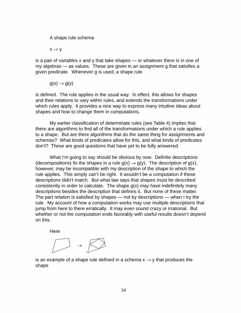
in the usual way. The computation begins with the shape C and ends with the shape D. Whenever a rule A → B is tried, a transformation t of A is taken away and the same transformation t of B is added back. But this is only the algebraic mechanism for applying rules. What’s interesting about the computation is what I can say about it as a continuous process, especially when parts are resolved in surprising ways. In the computation

37

��

��

in the algebra U1 2 a pair of squares is turned into a pair of triangles using the rule

that rotates a square, and the rule

that rotates a triangle. It sounds impossible, but it works. What parts do I need to account for this change, so that there’s no break or inconsistency? How are the parts the rules pick out related to one another? When do squares become triangles? And just what does it mean for the computation to be a continuous process?

I’m going to build on a configurational (combinatorial) idea that accords with normal experience to answer these questions. It’s the very idea I’ve been against all along as a way of handling shapes in computations. But the idea is indispensable when it comes to describing what happens as rules are applied. It’s important to keep this foremost in mind. There’s a huge difference between describing shapes and calculating with them. The latter doesn’t depend on the former. In fact, their relationship is just the opposite. The idea I’m going to use is pretty clear. Things are divided into a finite number of parts. I can recognize these parts — individually and in combination — and I can change them when I like for repair or improvement, or to produce something new. The parts I leave alone stay the same, and they keep their original relationships. Changes are continuous, so long as they correspond in this way to how things are divided into parts.

This idea can be stated in a far more general way with mappings. These describe what rules do to shapes, and relate their topologies (decompositions). The exact details of different mappings may vary — and it’s important when they do — but the core idea is pretty much as given above. Suppose a mapping from the parts of a shape C to parts of a shape C’ describes a rule A → B as it’s used to change C into C’. Then this process is continuous if two conditions are met.

(1) The part t(A) the rule picks out and replaces is in the topology of C. In terms of the intuitive idea above, the rule recognizes a part

38

that can be changed.

(2) For every part x of C, the mapping of the smallest part in the topology of C that includes x is part of the smallest part in the topology of C’ that includes the mapping of x. As a result, if two parts are parts of the same parts in the topology of C, then their mappings are parts of the same parts in the topology of C’. The rule changes the shape C to make the shape C’, so that the parts of C’ and their relationships are consistent with the parts of C. No division in C’ implies a division that’s not already in C.

The trick to this is to define topologies for the shapes in a computation, so that every rule application is continuous. This is possible for different mappings — each in a host of different ways — working backwards after the computation ends. (Of course if I’m impatient, I can redefine topologies after each step, or intermittently.) The mapping

h1(x) = x - t(A)

is a good example of this. It preserves every part x of the shape C - t(A) that isn’t taken away when a rule A → B is used to change a shape C into another shape C’. But mappings may have other properties. If the rule is an identity, then the alternative mapping

h2(x) = x - (t(A) - t(B))

works to include the previous scenario in this one. Now h2(x) = x, and every part of C is left alone. The computation is continuous if the topology of C is the same from step to step. In both cases, parts may not be fixed if there are more rules to try. What I can say about shapes that’s definite — at least for parts — may have to wait until I’ve stopped calculating. Descriptions are retrospective.

The third scenario is also easy to elaborate in useful ways. In particular, the topologies of the shapes in a computation can be filled out when identities are applied to extend the computation without changing its results.

Erasing and identity

Some easy illustrations show how these three scenarios work. Suppose I want to use the first scenario to define decompositions for the shape

39

�� ��

in terms of the two shape rules

that erase triangles and squares. rules are applied to produce an empty remainder. These are illustrated neatly in this way

by filling in triangles. the Boolean algebra that describes the shape. decompositions, four triangles and two squares are picked out as the atoms in Boolean algebras, and in the last decomposition, eight triangles are.

There are two interesting things to notice. illustrations in parallel computations — that is, in computations carried out in a direct product of algebras — by recapitulating the use of the rules

in the algebra U1 2

, and building up the corresponding decompositions in a combination of the algebras U

1 2 and U

2 2 , so that squares contain lines, and

triangles are planes. Alternatively, labeled lines or lines with weights fix the layers in this direct product.

1 2 and U

2 2 or of

W1 2

and U2 2

will do the whole job. The graphics is more concise, but perhaps not as clear. These

show my original idea. They are applied in the six step computation

�� ��

��

��

������������ ������������

�

�

Five distinct decompositions result when the

In the first decomposition, four squares are the atoms in In each of the three succeeding

First, I can produce the above

So a combination of the algebras V

I need two rules whatever I do.

40

� �

� �

� �

���� ���� ��� �����������

������� �������

to produce the third decomposition above. The rule used in each step of the computation is indicated by number. It’s easy to see that the sequence of rule applications could be different, so long as the same triangles and squares are picked out. In this scenario and the next one for identities, decompositions do not reflect the order in which rules are applied. The same rule applications in any sequence have the same result. But in the third scenario, decompositions may be sensitive to when rules are used.

Second, the number f(n) of different decompositions for any shape in the series

�����

can be given in terms of its numerical position n. The first shape in the series is described in one way — it’s a square — and the second shape can be described in two ways — it’s either two squares or four triangles. Moreover, the number of possible descriptions for each of the succeeding shapes — so long as I want the remainder to be empty — is the corresponding term in the series of Fibonacci

41

��

�� ��

numbers defined by f(n) = f(n-1) + f(n-2). It’s easy to see exactly how this works in the following way

��������������������������������������������

If a rule resolves the inmost square in the shape f(n), then there are f(n-1) ways to describe the remaining part of the shape — this part is one shape back in the series. Alternatively, if a rule resolves the four inmost triangles in the shape f(n), then there are f(n-2) descriptions — the remaining part is now two shapes back in the series. So the total number of descriptions is f(n) = f(n-1) + f(n-2). I can prove this for any square and any four triangles that include the square. Still, the visual proof is immediate enough to make the formal proof superfluous. Seeing is believing.

Now suppose I recast the rules

as the identities

��

and then use them to define decompositions according to the second scenario. Once again, consider the shape

If I apply an identity to pick out this triangle

and an identity to resolve this square

then the following topology (decomposition)

42

is defined. In this case, I have shown the topology as a lattice. It is easy to see that the right angle of the triangle and a corner of the square are distinguished. But other parts of the triangle and the square go unnoticed. If I recognize complements in addition to the parts I resolve when I use the identities, then a Boolean algebra is defined that has these four atoms

Now the triangle and the square have two parts apiece

Of course, I can always apply the identities everywhere I can. This determines another Boolean algebra with the 24 atoms

There are a couple of things to notice. Triangles come in three kinds

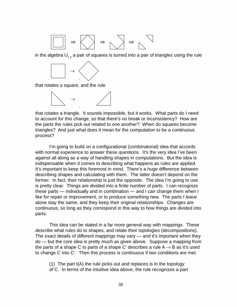
with three parts or four, and squares come in three kinds

with four parts or eight. Moreover, the different decompositions of the shape may be regarded as subalgebras of the Boolean algebra, including the above five decompositions obtained in the first scenario. But there’s no guarantee that

43

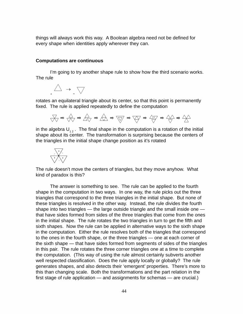
things will always work this way. A Boolean algebra need not be defined for every shape when identities apply wherever they can.

Computations are continuous

I’m going to try another shape rule to show how the third scenario works. The rule

��

rotates an equilateral triangle about its center, so that this point is permanently fixed. The rule is applied repeatedly to define the computation

in the algebra U1 2 . The final shape in the computation is a rotation of the initial shape about its center. The transformation is surprising because the centers of the triangles in the initial shape change position as it’s rotated

The rule doesn’t move the centers of triangles, but they move anyhow. What kind of paradox is this?

The answer is something to see. The rule can be applied to the fourth shape in the computation in two ways. In one way, the rule picks out the three triangles that correspond to the three triangles in the initial shape. But none of these triangles is resolved in the other way. Instead, the rule divides the fourth shape into two triangles — the large outside triangle and the small inside one — that have sides formed from sides of the three triangles that come from the ones in the initial shape. The rule rotates the two triangles in turn to get the fifth and sixth shapes. Now the rule can be applied in alternative ways to the sixth shape in the computation. Either the rule resolves both of the triangles that correspond to the ones in the fourth shape, or the three triangles — one at each corner of the sixth shape — that have sides formed from segments of sides of the triangles in this pair. The rule rotates the three corner triangles one at a time to complete the computation. (This way of using the rule almost certainly subverts another well respected classification. Does the rule apply locally or globally? The rule generates shapes, and also detects their ‘emergent’ properties. There’s more to this than changing scale. Both the transformations and the part relation in the first stage of rule application — and assignments for schemas — are crucial.)

44

The nine shapes in the computation

are all made up of triangles. Their numbers summarize the action of the rule as it is applied from step to step.

The first series shows the maximum number of triangles — these can be picked out using an identity — in each of the shapes. The next series gives the number of triangles in a shape after the rule has been applied, and the last series gives the number of triangles in a shape as the rule is being applied. cases, the number of triangles depends on what the rule does either by rotating an existing triangle or seeing a new one to rotate, and then counting in terms of the triangle and its complement. The resulting inconsistencies in the fourth and sixth shapes tell the story. and neither number is five. s blind luck that two and three make five. cases, there’s no easy relationship like this.) ation is a continuous process if appropriate topologies are given for the nine shapes.

____________________________________________________________

Table 6

Defining Topologies for Shapes in a Computation

Shapes

Atoms

���������������������������������

���������������������������������

���������������������������������

Consider the following three series

In both of these

Counting goes awry: two triangles just can’t be three, (It’ In many

Nevertheless, the comput

____________________________________________________________

45

The topologies for the shapes in the computation are defined as Boolean algebras with the atoms in Table 6. This is feasible using the above mapping h1(x) = x - t(A). First a topology is given for the final shape. Any finite topology will do. I’ve used the trivial topology — the final shape is an atom — because the rule doesn’t divide it. There’s not much for me to say. The final shape is vague without parts or purpose, but ready for more calculation. Once the topology of the final shape is decided, the topologies of the preceding shapes are defined in reverse order to keep the application of the rule continuous. Each topology contains the triangle resolved by the rule — the top most atom in Table 6 — and its complement. I can do this in different ways, with or without complements.

It’s instructive to keep a record of the divisions in the triangle in the right side of the rule

��

formed with respect to these topologies. The triangle is cut in alternative ways in the eight steps of the computation

The parts defined in the triangle combine sequentially to build up the different triangles that the rule picks out in its subsequent applications. The pieces

from the first three triangles combine in this way

and the remaining sides

combine in this way

to define parts (atoms) in the topologies of the second and third shapes in the computation, and ultimately the large outside triangle and the small inside one

46

in the topology of the fourth shape. Moreover, the pieces in the fourth and fifth triangles combine in like fashion to make the three triangles in the topology of the sixth shape that are needed for the production of the final shape. Looking forward, the topologies of the shapes in the computation appear to anticipate what the rule is going to do the next time it’s applied. But this is because the topologies are given retrospectively. Once a computation ends, I can always describe it as a continuous process in which shapes are assembled piece by piece in an orderly fashion. This makes a good story and a good explanation.

Every time the rule

��

is tried, its right side is divided with respect to a different topology. This shows in yet another way that the shapes in a rule have alternative descriptions that change as it’s used to calculate. But again, the rule doesn’t apply in terms of any fixed description. How the rule is described as it’s being used is just an artifact of the computation that may help to explain what’s going on.

Before I continue, it’s worth noting that the computation

is not isolated. There are many others like it. And in fact, they can be defined around each of the shapes in this infinite array of nested polygons

�����

�����

�����

�����

using only a single shape rule schema x → y, where x is a triangle or a regular polygon, and y is an appropriate transformation of x. The number of ways I can apply the schema to a shape in the array without remainder corresponds to the Fibonacci number of its column. This is described above for the series of squares inscribed in squares in the second row. Shapes are filled with

47

ambiguity. And there are always rules to take advantage of it in one way or another.

Decompositions are defined for a purpose. At the very least, they’re a nice way to talk about computations, and one way to explain what’s going on. But there’s a lot more. The decompositions that come from computations may describe shapes and provide the wherewithal to evaluate them when they are used in designs. Questions of function and use, manufacture and assembly, or repair and disposal are the kinds of things that can be addressed. This is often possible simply with rules that erase shapes or with identities. And many other things may also be involved, including any of the topological considerations — boundaries, complements, and so on — mentioned above. Moreover, stylistic analysis and the exploration of stylistic change rely on decompositions. Now they can be used to define new rules in terms of the scheme v ® A + B and its inverse. This provides some innovative ways to calculate with shapes. Already, there are clear applications in architecture and product design.

Most of what I’ve been saying about rules and computations with shapes is anecdotal. I’ve been presenting decompositions as case studies. This is no surprise. The way ambiguity is used in a particular computation may have little to do with the way it’s used in another. Ambiguity just won’t go away. It’s there whenever I apply shape rules to calculate. But it’s not handled in the same way all of the time. This is why ambiguity is so interesting, and why it’s so valuable. The trick is to use ambiguity without limiting it by trying to generalize. There’s no chance of this, so long as rules can vary as widely as shapes themselves. Shape rules fit the bill.

Design without thought

What is design? I used to agree wholeheartedly with Franz Reuleaux:

‘. . . Invention, in those cases especially where it succeeds, is Thought . . .’

But I’ve changed my mind. This is a dubious metaphor — even with Reuleaux’s optimistic qualification — if shapes play a role in design. The kind of reasoning shapes allow — the kind of reasoning William James describes as the ability to handle ambiguity and the novelty it brings — implies something more than the combinatorial, configurational, deductive, zero dimensional variety of thought Reuleaux takes for granted. Yet this is clearly computation. Reuleaux’s variety of thought is evident in expert systems and other computer models. Whatever these use — artificial intelligence and heuristic search, evolutionary algorithms

48

and optimization, formal logic, or common sense — they’re invariably going to be zero dimensional. (It appears this is an empirical fact. Nothing keeps me from using heuristics or optimizing when I calculate with shapes. However if evolution requires definite units, then evolutionary algorithms are limited to points. This bodes ill for more than design. Life itself may hang in the balance.) So what is design? Right now, I would say perception rather than thought. This is a provocative way to emphasize an important aspect of design. The creative activity I have in mind isn’t thought. Design depends on new ways of looking at things. This is exactly what shapes and computations with shapes are all about.

If I have tried to show anything in this chapter, it’s that shapes with points aren’t like shapes with lines, planes, and solids. Going from zero dimensional shapes to higher dimensional ones — from shapes where there are permanent units that I can count to shapes where unforeseen parts may pop in and out of existence whenever I look — alters almost everything. Identity and embedding simply aren’t the same, and counting may only discourage seeing. These are philosophical claims as much as algebraic or geometrical ones. I can always see things in new ways when I calculate with shapes made up of lines, planes, and solids. Shapes with points — and like devices whether decompositions or representations in computer models — limit what I can see and how much I can change my mind. Knowing how many points there are doesn’t make up for the loss. The last thing I want to do is count.

Is all this freedom really necessary? What do others say about design? The consensus among those who have thought about it is that design practice is flexible and open-ended. Donald Schon provides a good sense of this in his flattering account of the reflective practitioner. Schon puts ‘reframing’ and ‘back talk’ at the center of ideal practice in design and in other professions. This is the ability to interact with your work in the same unstructured way you argue about something new in vague and shifting terms that haven’t been defined. (When it’s finally time to define your terms, there isn’t very much to say.) It’s the ability to reconfigure what you’re doing before and after you act, to respond freely as you see things in different ways, and to try new ideas in an ongoing process whenever you like. This is what shape rules are for. Nothing prevents me from seeing triangles and K’s after drawing squares, and then acting as if that’s what was there all along. There’s no reason to assume I have to know anything definite before I see. When shape rules are used in computations, they meld redescription and inference. I can handle ambiguity and the flow of shifting interests and competing goals all at once. Multiple perspectives interact in intricate ways in the flux of practice. This provides the creative means to deal with new situations. Shape rules and the algebras in which they are defined promise a useful account of this kind of process.

49

Background

James Gips and I published the original idea for shape rules in 1972. Today, the literature on shape rules and the way they are used to calculate is much too large to cite item by item. Most of the relevant material has appeared in the journal Environment and Planning B: Planning and Design. Papers date from my first one in 1976 — ‘Two exercises in formal composition’ — in which I introduced the scheme v → A + B to define shape rules using spatial relations. These were enumerated from scratch, and fixed in decompositions formed by applying identities. The first use of shape rules to generate designs — Chinese ice-ray lattices — in a given style was described in my next paper the following year. With respect to the themes covered in this chapter, I would recommend papers by the authors in this list: alphabetically, Chris Earl (shape boundaries and topologies of shapes), Ulrich Flemming (architectural styles), Terry Knight (shape rules defined from scratch, stylistic analysis and stylistic change, and more), Ramesh Krishnamurti (computer implementations), Lionel March (miracles and what they mean), and myself. There are many other authors, though, and a lot more of equal interest.

The material from William James is in The Principles of Psychology (1981, pp. 957 - 958) in the chapter on reasoning. The section is aptly headed ‘In reasoning, we pick out essential qualities’. For James, the essential qualities of things may ‘vary from man to man and from hour to hour’ (p. 961). This is the same for shapes. Their parts are redefined every time a rule is tried. It strikes me sometimes that James is especially good at describing what happens when rules are used to calculate with shapes. This may be self-indulgent, but I can’t resist quoting him at length at least once. The following passage resonates perfectly with one side of what I’ve been saying about counting and seeing. (It doesn’t deal with the details of calculating that establish equivalences between complex things with numerable units and shapes without definite parts.)

‘The relation of numbers to experience is just like that of ‘kinds’ in logic. So long as an experience will keep its kind we can handle it by logic. So long as it will keep its number we can deal with it by arithmetic. Sensibly, however, things are constantly changing their numbers, just as they are changing their kinds. They are forever breaking apart and fusing. Compounds and their elements are never numerically identical, for the elements are sensibly many and the compounds sensibly one. Unless our arithmetic is to remain without application to life, we must somehow make more numerical continuity than we spontaneously find. Accordingly Lavoisier discovers his weight-units which remain the same in compounds and elements, though volume-units and quality-units all have changed. A great discovery! And modern science outdoes it by denying that compounds exist at all. There is no such thing as ‘water’ for ‘science’; that is only a handy name for H

2 and O when they have got into the position H-O-H, and then

affect our senses in a novel way. The modern theories of atoms, of heat, and of

50

gases are, in fact, only intensely artificial devices for gaining that constancy in the numbers of things which sensible experience will not show. “Sensible things are not the things for me,” says Science, “because in their changes they will not keep their numbers the same. Sensible qualities are not the qualities for me, because they can with difficulty be numbered at all. These hypothetic atoms, however, are the things, these hypothetic masses and velocities are the qualities for me; they will stay numbered all the time.”

‘By such elaborate inventions, and at such a cost to the imagination, do men succeed in making for themselves a world in which real things shall be coerced per fas aut nefas under arithmetical law.’ (p. 1250)

The cost to the imagination is twofold: there’s the effort to think up ‘elaborate inventions’, and then there are the limitations these put on what I can make of my future experience. I’m free to use my imagination anyhow I like when I calculate with shapes.

The quotation from Franz Reuleaux is in The Kinematics of Machinery (1963, p. 20). Donald Schon tells the story of the reflective practitioner every chance he gets. I like his account in Educating the Reflective Practitioner (1987) the most.

George Miller’s speculative comments at the beginning of this chapter are in his paper ‘Information Theory in Psychology’ in the omnibus volume The Study of Information: Interdisciplinary Messages, edited by Fritz Machlup and Una Mansfield (1983, pp. 495 - 496). Miller’s extension of the engineer’s idea of noise to cover ambiguity proves the value of the latter in creative work. How else could he invent the unlikely formula

ambiguity = noise

The equivalence, however, is within the ambit of common sense: ambiguity is just an annoyance that can always be removed. But shapes imply that both of the clauses in this statement are false. What do others have to say in Machlup and Mansfield’s book? Allen Newell (pp. 222 - 223) is unconcerned that units are used to describe things in computer models of thought. This is a ‘nonissue’ in computer science, at least for artificial intelligence. And Douglas Hofstadter (p. 270) thinks visual puzzles — IQ test problems of the kind invented by Alfred Binet and Lewis Terman — probe the mechanisms of intelligence. These are visual analogies, and may include those defined in shape rules and schemas. But according to Hofstadter, all visual puzzles aren’t alike. Some invented by other, less talented people — do they have lower IQ’s? — have the unfortunate property of being filled with ambiguity. Hofstadter wants to keep visual puzzles as experimental tools, and hopes to save them in the obvious way by removing any ambiguity. How is he going to do this, so that they’re still visual and useful?

51

What happens to rules and schemas? Despite their bickering in Machlup and Mansfield, both Newell and Hofstadter seem to be in agreement with Francis Galton. He had the idea of measuring mental ability before Binet and Terman. Galton never tired of saying, ‘Wherever you can, count.’ This becomes a habit that’s hard to break. But why start? You can count me out. There’s more to computation than counting. And there’s more to design with shapes. Seeing makes the difference. Shapes hold the creative choices ambiguity brings, so that decompositions, definitions, and the evanescent segments and shards of analysis are now afterthoughts of computation. Seeing makes it worthwhile to calculate with shapes.

Acknowledgement Mine Ozkar did a wonderful job on the figures. She also made sure I said something about everything I’d drawn.

Bibliography

Environment and Planning B: Planning and Design, 1976 - 2000, volumes 3 - 27.

James, William, 1981, The Principles of Psychology, Harvard University Press, Cambridge.

Machlup, Fritz and Mansfield, Una, 1983, The Study of Information: Interdisciplinary Messages, John Wiley & Sons, New York.

Reuleaux, Franz, 1963, The Kinematics of Machinery, Dover Publications, New York.

Schon, Donald A. 1987, Educating the Reflective Practitioner, Jossey-Bass Publishers, San Francisco.

52