1

How to build an economy free of recession: a new theory rising from the ashes of

both Keynesian and Neoclassical economics*

Samuel Meng, Institute for Rural Futures, UNE. Armidale, NSW2351

Abstract

Economic recession is a long-standing and often revisited topic. This paper argues

that all the existing studies and theories use aggregate macro models which fail to take

into account the market saturation phenomenon and thus fail to uncover the

fundamental cause of economic recessions. By including a saturation point for

consumption of each commodity, introducing the concept of the utility of savings, and

linking investment to profitability, the author has built a multi-commodity model to

study economic growth and business cycles. The modelling results show that, without

product innovation, the economy will reach a consumption and income ceiling so that

economic stagnation or a recession is inevitable. This suggests that the deficiency of

effective demand postulated by Keynesian economists actually comes from the supply

side – the scarcity of product innovation, or the imbalance between investment in

production innovation and investment in production. The author further shows that

cyclic product innovation leads to cyclic economic growth and that the scarcity of

product innovation may be due to the high possibility of innovation failure as well as

the problem of innovation imitation. In order to build an economy free of recession,

the paper calls for a thorough revision of the patent laws aiming at balancing the high

risk of innovation investment with a high return, and the formation of a functional

patent market, channelling funds automatically into innovation activities.

JEL code: E10, E20, E32,

Keywords: economic recessions, multi-commodity macro model, product innovation,

patent laws, economic growth

*This is an updated version of a previous working paper entitled ‘Unlocking the

mystery of economic recession using a multi-commodity macroeconomic model’.

2

How to build an economy free of recession: a new theory rising from the ashes of

Keynesian and Neoclassical economics

1. Introduction

Economic recessions continue to haunt mankind but the causes for recessions are not

yet fully understood. Ongoing research into the causes of economic recession is

imperative, because recession can have a significant negative impact on the

development of nations, as well as on the living standard of mankind. The effects of

large economic recessions can be quite devastating. During the Great Depression of

the 1930s, the output of several Western nations fell by 25-30% in the period between

1929 and 1932-33. In the United States (US), the unemployment rate peaked at 25%

in 1932-33, and it took almost a decade for US output to return to its pre-1929 level.

More recently, the Global Financial Crisis (GFC) and the current European Debt

Crisis are striking examples of the recurrence of economic recessions. During the

GFC, the US Dow Jones Industrial Average index dropped to a trough of less than

6,600 points in March 2009, from its peak of more than 14,000 points in October

2007. In the last quarter of 2008, US quarterly real GDP decreased by 8.9%. The

unemployment rate in the US increased from 4.6% in 2007 to 10.1% in 2010. As a

result of the European Debt Crisis, many nations in Europe also experienced high

levels of unemployment. According to the European Commission (2013),

unemployment rates in 2012 were 25.0% in Spain, 24.3% in Greece, 15.9% in

Portugal, and 14.9% in Cyprus. These statistics may not be instantly appealing

emotionally. However, with the media suggesting that some families became

homeless due to foreclosures or evictions and that parents had to beg for food for their

children, the consequences of recessions such as this one are clearly not only

economic but also psychological.

The negative impact of economic recession has triggered a considerable amount of

research. It is easy to explain recessions accompanied by commodity shortage, e.g.

recessions caused by wars, natural disasters, and impropriate government regulations.

However, recessions accompanied by the abundance of commodity are much harder

to comprehend and explain. A universally agreed-upon explanation and solution for

3

this phenomenon has yet to be developed. This becomes the motivation for this paper.

To uncover the fundamental cause of economic recessions, the author has proposed

several axioms based on common wisdom, and has developed a multi-commodity

macroeconomic model. The model preserves the Classical assumption for an economy

– the perfectly competitive market – and can provide a simple and universal

explanation for recurrent economic recession and for cyclical economic growth.

The remainder of the paper is organized as follows. Existing theories on economic

recessions and growth are briefly reviewed and discussed in Section 2. Based on

observations and reasoning in the real world, Section 3 identifies a series of axioms

which are critical to the model. In Section 4, the model is developed and explained.

Section 5 reveals the implications of modelling results for both commodity and factor

markets are analysed and the unique role of product innovation in both business

cycles and economic growth. The reasons for product innovation scarcity and the

ways of encouraging innovation are also discussed briefly in this section. Finally,

Section 6 summarizes the paper and provides brief concluding comments.

2. Major existing theories on economic recessions and growth

There are many studies on economic recession, so it is not possible or even necessary

to review them all in this paper. Instead, the author will review studies in this area on

the basis of various schools of economic thought. Since it is outside the scope of this

paper to discuss fully the theories underpinning previous research in this area, the

author will review and comment on only key concepts relevant to this paper.

Arguably the most influential study on economic recession was completed by Keynes

(1936) and carried further by his successors, labelled ‘Keynesian economists’ (either

‘old’, ‘orthodox’, ‘new’, or ‘post’). The main contribution of Keynesian economics to

explaining economic recession was shown by the concept of deficiency of effective

demand. Keynes attributed this deficiency to decreases in investment. He

demonstrated that a decrease in investment would lead to a proportionally greater

decrease in output through a multiplier effect. Keynes determined the most important

causes of this investment shortage to be, firstly, a lack of ‘animal spirits’

(entrepreneurship), and secondly, the liquidity preference, or the speculative motive to

hold cash in a world characterized by uncertainty (the ‘uncertainty argument’). On the

4

factor market, Keynes attributed high unemployment during a recession to the

fluctuations of expected profit (or ‘marginal efficiency of capital’ in Keynes’ words),

resulting from unstable investment expenditure. The liquidity preference and

uncertainty argument was further developed by post-Keynesian economists (e.g.

Davidson, 1984, 1991), while new microeconomic foundations were developed by

new-Keynesian economists, including the ideas based on real and nominal wage

rigidity, price rigidity, efficiency wages, etc. (e.g. Mankiw, 1985, 1989, Akerlof and

Yellen, 1985, Romer, 1993).

Keynesian economists intuitively identified that the key features of an economic

recession are depressed demand and high rates of unemployment. Their reasons for

highlighting these features were, however, quite unusual, e.g. liquidity preference and

the lack of entrepreneurship (by Post-Keynesian economists), and wage and price

rigidity in an economy (by New-Keynesian economists). The question unanswered by

Keynesian economists is why these factors exist during a recession but not exist in an

economic boom? In other words, Keynesian economists have not gone far enough to

uncover the causes for liquidity preference and the lack of entrepreneurship and to

work out the impact of wage and price rigidity under different circumstances.

Keynesian economists discarded the long-standing assumption of Classical economics

that perfectly competitive markets exist. By rejecting the existence of Adam Smith’s

‘invisible hand’ (i.e. the efficiency of the market), the solution by Keynesian

economists became one of interventionism.

Classical economics (Old, New, or Neo) is the main alternative to Keynesian

economics in explaining economic recession. Classical economists have great faith in

the efficiency of market mechanisms and in perfectly competitive markets. They

regard economic recessions as large natural economic fluctuations (e.g. Lucas, 1975,

Kydland and Prescott, 1982, Plosser, 1989, Prescott, 1986). They believe that, if

market forces were allowed to operate alone, economic recessions would be

temporary or relatively short-lived. Consequently, they argue that government

intervention is unnecessary. This argument has a valid point in that every recession

does lead to eventual recovery, although Keynesian economists might argue that this

occurs as a result of government intervention.

5

However, classical economists tend to deny or ignore the important features of

economic recession highlighted by Keynesian economists. The real business cycle

model, for example, view economic recessions as economic fluctuations caused by

supply side shocks like a decrease in productivity, a hike in oil prices, and a decrease

in labour supply. The model includes and explains none of the main features of an

economic recession such as stagnant demand, unutilized capital, and high

unemployment. These features indicate clearly that an economic recession is a

problem on the demand side: the economy has plenty of resources (e.g. unemployed

capital and labour) and capacity to produce but the sales stagnate. It is palely argued

by classical economists that the appearance of oversupply is due to the over-

production by high cost firms or to the production mismatching the consumers’

demand, and that the high unemployment is due to inflexible wages or voluntary

unemployment. Even if these far-fetched arguments are true and thus an economic

recession can be viewed as an economic disequilibrium, the question faced by

classical economists is why an efficient market allows this disequilibrium to last for

years or even for a decade? Classical economists have to admit either the market is

inefficient or a recession is not simply disequilibrium. In either way, classical

economists will contradict their own belief. By describing economic recessions as

natural fluctuations, however, classical economists avoid the task of finding the

causes of economic recessions and have failed to explain why an efficient market

allows some economic recessions to last for many years. Instead, they focus on

developing economic models and econometric estimations and choose to be

indifferent to the economic and psychological damage of a recession on human beings.

The classical economics solution to economic recession – natural recovery – is

unpopular with government and public alike.

The majority of economists today are neither strictly Classical nor strictly Keynesian.

Instead, most appear quite happy to accept the idea that the force of aggregate supply

stressed by Classical economists is more important in the long run, while aggregate

demand emphasized by Keynesian economists plays a key role in the short run

(Sorensen and Whitta-Jacobsen, 2010). Thus, the dichotomy between Keynesian and

Classical economics evolves as a dichotomy between the long run and the short run.

That is, conflicting theories are being applied to the same economy but from different

perspectives. Economists in this dichotomous camp have to believe, however, that the

6

long run aggregate supply is a vertical line, i.e. an infinitely inelastic supply curve.

Without a vertical long run aggregate supply curve, the dichotomy between the long

run and the short run will break down.

When one seeks to uncover the microeconomic foundation for this vertical long run

supply curve, the opposite appears to be the case: a vertical supply curve for a firm or

an industry is found only in the case of a very short run. In the long run, an industry

supply curve can be increasing, constant, or decreasing, depending on the nature of

the industry. In considering that an economy has many different kinds of industries,

the long-run aggregate supply curve for an economy can be viewed as a combination

of supply curves for all industries. Therefore, the aggregate long-run supply curve

should be similar to the moderated form of long-run supply curves for the industry,

and thus it can never be a vertical line.

Supporters of the dichotomy between the long run and short run may argue that the

vertical aggregate supply curve indicates limited resources in the long run. However,

this begs two questions. First, why can there not be resource limitations in the short

run? In fact, resource limitations have occurred in many periods throughout history,

and can be found either in the long run or in the short run. Secondly, what about the

effect of technological progress? It is widely accepted that technological progress is a

significant factor in the long run and that it can empower firms to increase their output

with limited resources. In the light of this, the limited resource will not cause capped

supply in the long run. In short, a vertical aggregate supply curve in the long run

cannot be employed to conciliate Keynesian and Classical economics1.

Marx’s explanation of economic recession has been given little attention in economics

literature, perhaps because of his radical idea of advocating class warfare. Nonetheless,

there is an element of truth in the Marxist argument that warrants discussion here.

Marxists determine that economic recession is caused by inequality. Their explanation

is based on their observation of overproduction in the economy as well as the

1 The argument can be more complicated if one thinks that the impact of money supply on aggregate

supply curve for the economy, namely, the price level for an aggregate supply curve indicates the

relative price between goods and money so it is influenced by money supply. Here we discuss the real

economy rather than the nominal one, so the impact of monetary policy can be excluded by fixing

money supply. As such, the aggregate supply curve reflects the relationship between the real price level

and the amount of goods supplied, so the aggregate supply curve has meaning similar to the supply

curve for an industry or for a firm.

7

considerable income gap between the rich and the poor. They argue that capitalists

push wages down and raise the rate of surplus value, and that this causes excess

supply and inadequate aggregate demand. There is little doubt that income

distribution inequality plays an important role in economic recessions. The GFC

strongly illustrated the importance of income inequality in economic recessions.

Large-scale lending by the rich to the poor boosted demand for housing and

consumption but, when the rich sense a risk of loan default and want their loans

repaid, the resulting financial constraint on the poor and thus the consequent decrease

in final demand pushes the economy into recession. While it is therefore clear that

income inequality is a contributing factor to economic recession, income inequality

may not be a fundamental factor underpinning recession. Given the large production

capacity for almost every available commodity in the modern global economy, there

is always a possibility for overproduction and thus deficiency of demand, even if

income is equally distributed and everyone has sufficient income to buy what they

want. So, income inequality can aggravate or accelerate a recession, but it is not a

fundamental cause.

From the above discussion it is clear that previous studies of economic recession hold

some elements of truth. However, they have failed to uncover the fundamental cause

of recession, and thus have failed to provide a satisfactory solution. As long as

economic recessions continue to occur, the search for answers must also continue.

3. The rationale of the new theory

Based on the forgone discussion, the existing theories on economic growth and

business cycles disagree with each other. The classical theories (e.g. the real business

model, the balance growth model and the endogenous growth model) focus on the

supply side while the Keynesian and Marx’s theories focus on demand side. However,

there is a common feature in all these theories: all of them are based on aggregate

macro models (e.g. Keynes’ multiplier model, the AS/AD model, the real business

cycle model and the endogenous growth model). These highly aggregated models

have insufficient information on both production and consumption so that they fail to

reveal the links between supply and demand. The new theory tends to take into

account both the supply and demand sides and uncover the links between them. To

this end, this study uses a multi-commodity macroeconomic model.

8

The basic rationale of the new theory is as follows. In the absence of a new product

(or in the case of very slow product innovation), the saturation point of each type of

commodity necessitates a consumption ceiling. Since the profit from investment is

achieved eventually from selling products to consumers, the consumption ceiling

necessitates an investment ceiling. When the economy reaches both consumption and

investment ceilings, stagnation and/or recession are inevitable. Product innovation is

the key to the recovery from the recession and to the economic growth. This rationale

is crucially based on three simple axioms which are based on real world observations

and commonly accepted norms, so the focus of this section is to discuss these axioms.

Axiom 1: every commodity has a saturation point for each individual.

In accepted preference and utility theory, it is assumed that consumers always prefer

greater quantities of any kind of commodity. That is, the greater the quantity of

commodities consumed, the higher utility will be. This assumption, ‘the more is

better’, is easily understood and widely accepted, but it is not applicable without

conditions. For example, most people like ice cream and, generally speaking, the

more ice cream consumed, the higher utility. Eating too much ice cream will, however,

lead to vomiting or stomach pains. This example can be generalized to any good and

service, and suggests that overconsumption can be a burden for a consumer.

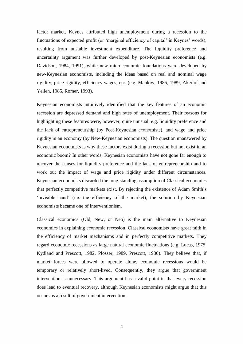
The above example demonstrates that a satiation point exists for the consumption of

any commodity (here the concept of consumption is strictly defined as the use-up of

goods or services)2. If the amount of consumption surpasses the satiation point, the

utility from consumption will decline. To embody the satiation point in the utility

function, a parabolic utility function is proposed:

2( ) 2U x mx x

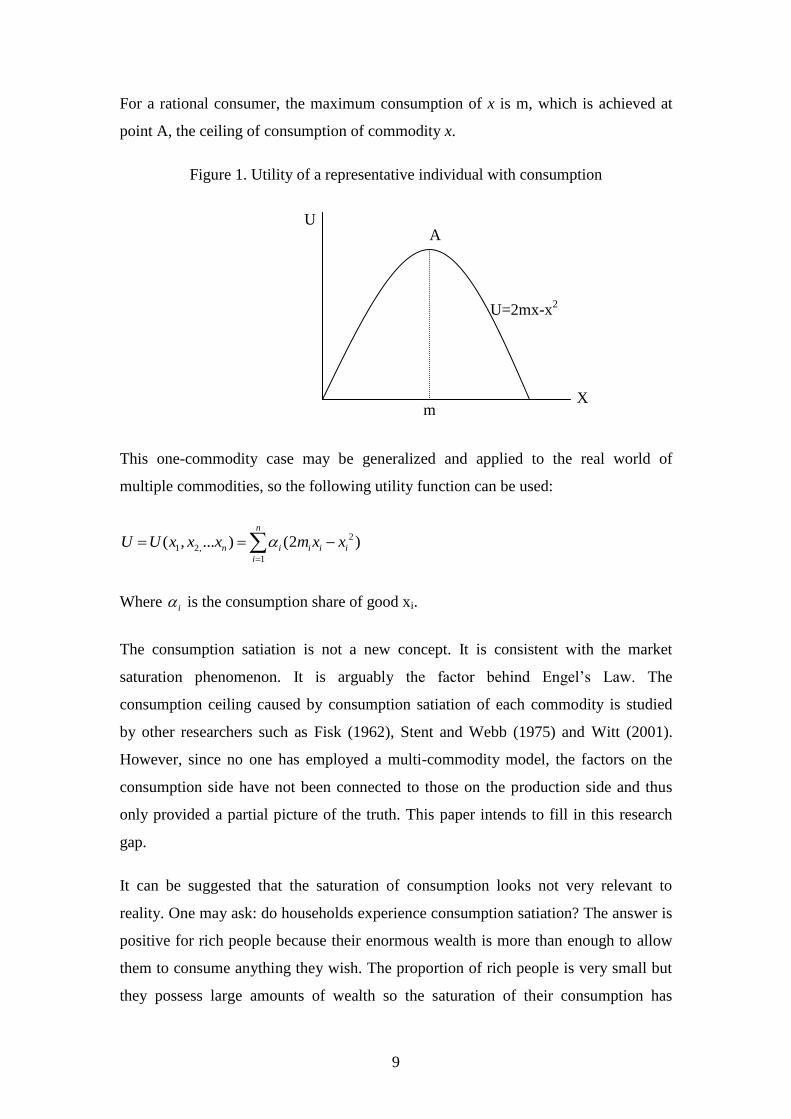
This utility function is illustrated in Figure 1. When the amount of consumption of x is

less than a, the utility achieved increases as the consumption increases. Once x is

greater than a, however, further increases in consumption will result in lower utility.

2 It is arguable that consumption can include commodities purchased for future use or for others’ use

(e.g. gift, donation or bequeathing). This type of consumption can be treated either as other people’s

consumption if the commodity is used up, or as other people’s savings if the commodity is unused by

other people, which will be discussed next.

9

For a rational consumer, the maximum consumption of x is m, which is achieved at

point A, the ceiling of consumption of commodity x.

Figure 1. Utility of a representative individual with consumption

This one-commodity case may be generalized and applied to the real world of

multiple commodities, so the following utility function can be used:

2

1 2,

1

( , ... ) (2 )n

n i i i i

i

U U x x x m x x

Where i is the consumption share of good xi.

The consumption satiation is not a new concept. It is consistent with the market

saturation phenomenon. It is arguably the factor behind Engel’s Law. The

consumption ceiling caused by consumption satiation of each commodity is studied

by other researchers such as Fisk (1962), Stent and Webb (1975) and Witt (2001).

However, since no one has employed a multi-commodity model, the factors on the

consumption side have not been connected to those on the production side and thus

only provided a partial picture of the truth. This paper intends to fill in this research

gap.

It can be suggested that the saturation of consumption looks not very relevant to

reality. One may ask: do households experience consumption satiation? The answer is

positive for rich people because their enormous wealth is more than enough to allow

them to consume anything they wish. The proportion of rich people is very small but

they possess large amounts of wealth so the saturation of their consumption has

X

U A

U=2mx-x2

m

10

substantial impact on the economy. Although poor people have not reached their

consumption saturation points, the contribution of their consumption to the economy

is unlikely to increase if the unequal income distribution in the economy is not to be

changed. In other words, they have reached their lower financially-constrained

consumption ceilings. When one thinks about the massive production capacity in a

modern economy, it is on the right track to say that the majority of products in the

markets – the old products – tend to reach or approach the consumption ceiling.

The other argument may be that, in the case of an open economy, the untapped

markets in developing countries make consumption satiation less relevant. It is true

that entering markets in developing countries will moderate the pressure of

consumption satiation in developed countries, but the problem of consumption

satiation cannot be avoided. One reason is that the markets in developing countries

will be saturated eventually. The other reason is that, given the low income in

developing countries, the exports into these countries will be further limited by the

purchasing power of these countries. Therefore, consumption satiation is a problem

both in theory and in reality.

Axiom 2: saving can generate utility directly and immediately.

Saving is traditionally treated as future consumption plus some interest income from

the saving, so it is normally not included in a utility function. The theory behind this

practice is the life cycle theory developed by Modigliani and Brumberg (1954) and

Modigliani (1986), and the permanent income theory developed by Friedman (1957).

Both studies utilized the intertemporal choice model developed by Fisher (1930).

Since this model is still popularly used to explain the saving and borrowing behaviour

and many dynamic macro models are based on this model, it is useful to introduce the

rationale of this model and point out the fundamental flaw in the model.

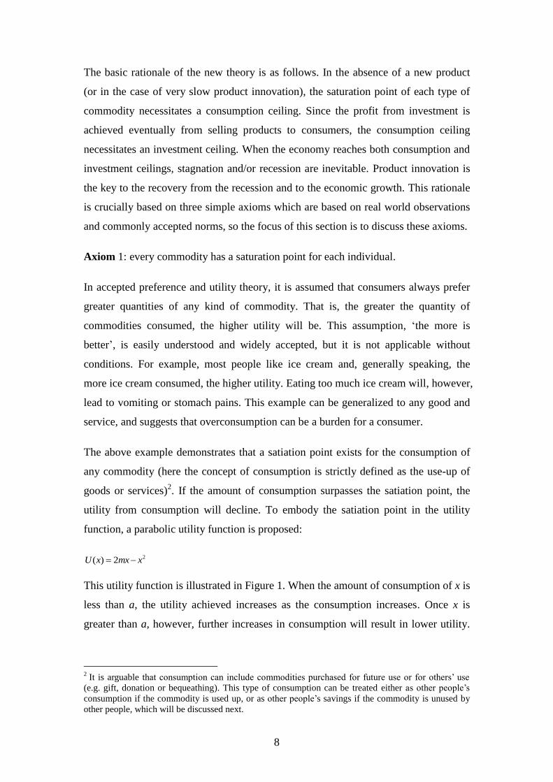
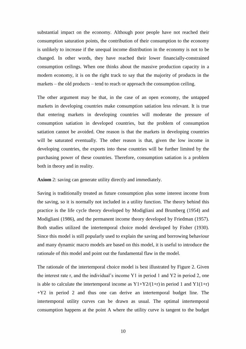
The rationale of the intertemporal choice model is best illustrated by Figure 2. Given

the interest rate r, and the individual’s income Y1 in period 1 and Y2 in period 2, one

is able to calculate the intertemporal income as Y1+Y2/(1+r) in period 1 and Y1(1+r)

+Y2 in period 2 and thus one can derive an intertemporal budget line. The

intertemporal utility curves can be drawn as usual. The optimal intertemporal

consumption happens at the point A where the utility curve is tangent to the budget

11

line. If Y1>C1, the individual will choose to save in period 1 and to utilize the saving

in period 2. On the other hand, if Y1<C1, the individual will choose to borrow against

the future income and keep the consumption level C1, and to pay back at period 2.

Figure 2 The rationale of intertemporal choice model

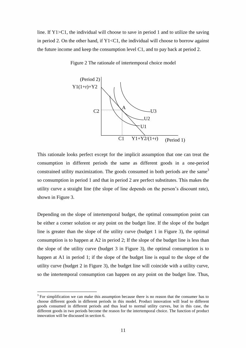
This rationale looks perfect except for the implicit assumption that one can treat the

consumption in different periods the same as different goods in a one-period

constrained utility maximization. The goods consumed in both periods are the same3

so consumption in period 1 and that in period 2 are perfect substitutes. This makes the

utility curve a straight line (the slope of line depends on the person’s discount rate),

shown in Figure 3.

Depending on the slope of intertemporal budget, the optimal consumption point can

be either a corner solution or any point on the budget line. If the slope of the budget

line is greater than the slope of the utility curve (budget 1 in Figure 3), the optimal

consumption is to happen at A2 in period 2; If the slope of the budget line is less than

the slope of the utility curve (budget 3 in Figure 3), the optimal consumption is to

happen at A1 in period 1; if the slope of the budget line is equal to the slope of the

utility curve (budget 2 in Figure 3), the budget line will coincide with a utility curve,

so the intertemporal consumption can happen on any point on the budget line. Thus,

3 For simplification we can make this assumption because there is no reason that the consumer has to

choose different goods in different periods in this model. Product innovation will lead to different

goods consumed in different periods and thus lead to normal utility curves, but in this case, the

different goods in two periods become the reason for the intertemporal choice. The function of product

innovation will be discussed in section 6.

C1

U3

U2

U1

(Period 1) Y1+Y2/(1+r)

Y1(1+r)+Y2

C2 A

(Period 2)

12

the whole model collapses because it fails to explain the saving and borrowing

behaviour.

Figure 3 The rationale of intertemporal choice model

The intuition behind this result is as follows. Since the slope of intertemporal utility is

determined by the individual’s discount rate and the slope of the intertemporal budget

line is determined by the interest rate, due to the perfect intertemporal substitution

effect, the saving and borrowing behaviour will be determined by the difference

between the interest rate (implied by the slope of the budget line) and the individual’s

discounting rate (implied by the slope of the utility curve): if the two rates are the

same, the person will be indifferent in consuming in period 1 or period 2; if the

person’s discount rate is higher than the interest rate, he/she will borrow and consume

all his/her income in period 1 and vice versa.4

In short, although saving will lead to future consumption, treating saving as future

consumption is not adequate in modelling the saving decisions of households because,

in the real world, future consumption is not the only reason for savings behaviour.

There are many other motives for saving money. A good example of this is the

phenomenon that so many billionaires, who already have more than enough money

for future consumption potential, continually seek to increase their wealth and

therefore their savings. Moreover, the notation of future consumption in lifecycle and

4 It is arguable that one must consume the same good (e.g. food) in both periods. In this case, the

consumption in two periods can be divided into two parts, the fixed proportion part and the perfectly

flexible part. The fixed proportion part is irresponsive to interest rates and the perfectly flexible part is

either corner solution or undetermined, so the intertemporal choice model is still unable to explain the

household consumption behavior.

A1

U3

U2

U1

(Period 1)

A2 Budget 3

(Period 2)

Budget 1

Budget 2

13

permanent income theories is not so useful for a realistic model. Analytical models

based on this concept, such as the Ramsey-Cass-Koopmans model (Ramsey, 1928,

Cass, 1965, Koopmans, 1965) are not applicable in the real world. This is because the

future is full of uncertainty. Nobody can foresee future income, future consumption,

or an individual’s life span. So, how can an individual make savings decisions using

the lifecycle and permanent income hypothesis? Given that the future cannot be

foreseen, the best practice is therefore to save as much as one can.

Treating saving as future consumption also ignores the difference between saving

action and the amount of goods saved and thus ignores the utility generated from the

saving action. It is important to differentiate saving action from savings (the amount

of goods saved), consumption action from the goods consumed. Strictly speaking, it is

the consumption action that generates utility, e.g. the taste of food and the energy

obtained in the consumption of food. Since the goods will vanish after the

consumption action, it is not essential to differentiate these two concepts, i.e. we can

say either consumption action generates utility or the goods consumed generate utility.

However, it is a different story with saving because the goods saved will not vanish

during the saving action. Although the amount of utility from saving may be

positively related to the amount of goods saved, the utility of saving comes directly

from the saving action instead of the goods saved. The goods saved cannot generate

any utility during the saving action but they can generate utility in the consumption

action in the future. In a nutshell, the utility of saving comes from the saving action

while the utility generated by the saved goods is captured by the consumption

function of the future.

Since saving behaviour cannot be modelled accurately by treating savings simply as

future consumption, the only practical way to model savings is to place it directly in

the utility function. As a particular type of goods, savings do in fact generate utility

directly, and this utility underpins household saving behaviour. There are a number of

utility-related motives for saving action. The first of these is precautionary saving.

That is, savings can avoid or minimise hardship during unforeseen difficult times, and

so savings behaviour can give the individual a sense of security. Second, the amount

of saving (or wealth) reflects the social status and power of the individual, and it is

from this status that some individuals derive considerable satisfaction. Third,

14

individuals can obtain profits from astute investment of their savings, and investment

profit is pleasurable for many individuals. Fourth, savings can be used to obtain goods

and services that are not currently available, but which are expected to be available in

the future. Knowing that one is in a good position to enjoy new products in the future

can also generate satisfaction. Finally, savings (and other wealth) can be passed on to

offspring, bringing pleasure to those making the savings. The multiple purposes of

saving are not exclusive to each other. For example, if an individual saves for rainy

days, he can also put his saving into his bank and thus earn some interest.

From these savings motivations we can claim that savings can generate utility directly

and thus they should be put in the utility function. Actually, including savings in a

utility function is not a novel practice. For example, Howe (1975) treated saving as a

good in a linear expenditure system. In so doing, Howe derived the same extended

linear expenditure system as developed by Lluch (1973), who used an intertemporal

utility maximization of the Stone-Geary utility function. What the author suggests in

this paper is that savings must be included in the utility function to take into account

the utility generated by saving action. Putting it differently, there are two kinds of

utility related to savings. One is the utility from the saving action and the other is the

utility from the future consumption of saved goods. The former enters the utility

function as savings and the latter enters the utility function as consumption in

different periods.

The amount of utility generated by the action of saving at the present time is

positively related to the amount of saving, i.e. the more one saves, the more

satisfaction one obtains. Unlike ordinary goods, there is no ceiling for savings, so the

concept of ‘the more is better’ applies with no constraint. A number of functions can

be used to describe the utility of saving action. For simplification, we use a linear

function for the utility of saving: ( ) *SU Savings Savings . This utility function of

saving also allows negative saving (dissaving) to generate negative utility. In

considering all factors affecting household utility, the following utility function is

created:

2

1 2,

1

( , ... , ) (2 ) *n

n i i i i S

i

U U x x x Savings m x x Savings

15

The additional benefit of putting savings into a utility function (e.g. the above utility

function) is that the amount of saving is determined by the consumer’s utility

maximization decision, rather than mechanically linked to income level as in many

existing aggregate macroeconomic models.

There may be some arguments against putting saving into a utility function. One such

argument is that, if savings generate utility and dissavings generate negative utility,

how can you explain why so many households utilise debt (e.g. housing mortgage

loan)? People raising this question only see the one type of utility related to savings –

the utility generated from saving action. In the case of household debt (dissaving), the

utility related to dissaving action is negative, but the dissaving allows the household

to consume more in this period. As long as the utility from the increased consumption

outweighs the negative utility from dissaving action, the utility increases when the

household borrows. As a result, the rising household debt phenomenon does not

disapprove the practice of putting saving into a utility function.

Another argument may be that, for some people who never save, savings may

generate little utility (or have little value) and thus it is meaningless to put saving into

a utility function. Clearly, household saving behaviour is complex. Due to the benefits

of saving described above, most people prefer to have savings, but some individuals

do prefer to spend all their wealth. In this case, the amount of saving is negligible, and

thus the saving component in the utility function is of little importance. We can also

assign a very small value (even zero) for the weight on saving ( S ) for these

individuals. Thus, the utility function is still valid in these circumstances. It is widely

accepted that individual saving is arguably more common amongst Asian people than

those from Western societies, given the weaker economic safety nets available in most

Asian nations. In this case, the strong safety nets of Western nations can themselves

be considered collective or compulsory savings, in the form of pensions, social

security funds, and superannuation funds. Consequently, these forms of savings

provide utility for all people in the country. Since almost all people can derive utility

directly from savings (either individual, collective, or compulsory, or a mixture of all

three types), it is necessary to include savings in the utility function.

There may be other arguments against including savings in a utility function from the

angle of rigorousness of a theory. One may say this practice violates the neutrality of

16

money, a doctrine of Classical economics. It must be noted that savings in the above

utility function refers to real savings. Real savings can be calculated as nominal

savings divided by the price level. Alternatively, real savings can also be calculated as

the sum of all kinds of unconsumed (saved) commodities, i.e. 1

n

i

i

Savings S

. Using

this second approach, it is easy to dismiss concern that including saving in a utility

function may violate the neutrality of money.

One may also be worried that this practice will cause double counting when the

savings are spent, or it may imply that there is always general overproduction in the

economy because some output is not consumed (that is, it is saved). The former

argument results from the old thinking: the utility of saving results from future

consumption. When the utility of saving is viewed as satisfaction from saving action

(i.e. holding savings for various purposes), the utility from spending of savings is the

utility of consumption in the future, rather than the utility of saving action. Therefore,

if savings are used, the utility of consumption of goods in the proposed utility

function increases while the utility of saving decreases. Consequently, the utility

function is consistent at all time. Regarding the latter argument, overproduction is

indeed possible given this utility function but is not always present. The key to this

lies in whether or not savings can be fully utilised. This is related to the axiom

regarding investment demand, which will be discussed next.

Axiom 3: investment demand is determined by consumption growth potential.

The traditional investment theory (e.g. the loanable funds theory) claims that a

flexible interest rate can always make sure that the supply of savings is equal to the

demand for investment, thereby producing equilibrium in the capital market5

.

Keynesian economists reject this theory based on liquidity preference, which rejects

the neutrality of money, the core assumption of neoclassical economics. Actually,

5 In this case we are considering the pure market situation, without government interference in interest

rates. Even with government intervention (by setting official interest rates through a central bank), the

nature of the capital market does not change. Practically, most official interest rates are indicative only,

so commercial banks are not necessarily required to follow the official lead. Even in the case of

enforceable official interest rates, the shadow or underground banking system will often circumvent the

official requirement. Theoretically, an inappropriate official interest rate may cause excess demand or

supply, but will not result in a shift of the supply and demand curve. Thus it will not become the

equilibrium interest rate. The equilibrium interest rate is determined endogenously.

17

even with the assumption of neutrality of money, the loanable funds theory may not

hold.

To make sure that the saving supply and investment demand are equal, one must

accept that, when the interest rate decreases, the investment demand curve will be

bent to the right so that it will never meet the horizontal axis. Otherwise, it is possible

that the investment demand curve intersects the horizontal axis earlier (at a lower

quantity) than the savings supply curve intersects the horizontal axis. This means that

the investment demand cannot absorb all the saving supply even if the interest is zero.

The reasoning of a bent investment demand curve is similar to the argument of Pigou

(1943) on Pigou effect and Keynesian effect in the case of the aggregate demand

curve. However, an investment demand curve bent to the right implies that the interest

rate can affect investment demand exogenously, but this contradicts the fact that

interest rates are an endogenous factor. That is, supply of savings, demand for

investment and interest rates affect one another and are determined simultaneously6.

Therefore, it is not guaranteed that the investment demand curve can always intersect

the horizontal axis at a quantity larger than the savings supply when interest rate is

zero, and thus the equilibrium in the capital market may not be achieved.

To illustrate this point, a simple saving and investment equilibrium graph is employed.

In Figure 4, the horizontal axis is the amount of saving or investment and the vertical

axis is the interest rate. The investment curve I is a standard one – a downward

sloping line. The saving curve S is upward sloping but with a starting point on the

horizontal axis. This setting is to reflect the fact that, due to not-for-profit purposes of

saving (e.g. precautionary saving), there is a minimum amount of savings even if the

interest rate is zero. The effect of the official setting of the interest rate is to cause

investment demand to move along the investment curve. For example, if the Reserve

Bank sets the interest rate too high at ih, the level of investment will be below the

level of saving and this will lead to a monetary-policy-led contraction. On the other

hand, if the reserve bank sets the interest rate too low at il, the level of investment will

be higher than the level of saving and this will lead to a monetary-policy-led

6 If one insists that the interest rate is exogenous because it is set by a central bank, then the supply

curve must be either absent, or identical to the horizontal interest rate line. This contradicts the

assumption of loanable funds theory.

18

expansion. In short, an impropriate setting of official interest rates leads to an artificial

fluctuation of the economy, or unbalanced economic growth.

Figure 4. The possibility of uninvested savings

For simplicity, assuming the Reserve Bank is capable of setting the official interest

rate at the equilibrium interest rate so that S=I, or saving is fully invested. This

equilibrium is, however, achieved only under the condition that there are plenty of

investment opportunities, or the profitability of investment is good. If the investment

profitability is low, the investment curve will pivot left from I to I’. This leads to a

lower level of investment and lower equilibrium interest rate. When the investment

profitability is approaching zero or even becomes negative, or the risk of investment

is very high, the investment curve will pivot further left to I’’. In this case, the

investment curve will not meet the saving curve. This means, even if the interest rate

is zero, the amount of saving will not be fully invested. The rationale behind this is

that, in the time of no investment opportunity or of high risk of investment, it is better

for the investor to hold cash rather than to invest and thus make a loss.

The endogenous nature of interest rates means that they cannot be a determinant of

investment demand. Consequently, a truly exogenous determinant must be found.

This is not a difficult task when one considers the purpose of investment: to obtain

profit. As Tobin (1969) noticed, investment demand depends critically on profitability.

A further thinking reveals that the profitability is in turn dependent crucially on final

demand.

Q

i

I’’

S

I’

I

S0

ih

il

19

We think about the case of investment in production first. The profitability of an

investment is determined by both cost of, and revenue from, an investment. On the

cost side, interest rates, wages and prices on intermediate inputs are important factors.

However, these prices (including interest rates and wages) are determined by supply

and demand. The supply side is determined by technology and resources which are

exogenous and thus out of the control of mankind7. The demand side (intermediate

demand) is ultimately determined by the final demand because the ultimate purpose of

production is to cater for the final demand. So, the final demand has crucial influence

on cost side. On the revenue side, investment income is achieved through sales of

output to both intermediate demand and final demand. Since the sales to intermediate

demand is to cater for the final demand, the final demand for output will determine

both price and the quantity of sales made. There are many kinds of final demand such

as household consumption, government consumption, exports, and investment

demand. Household consumption, government consumption, exports simply reflect

consumption by different consumer groups, so they can be grouped under a broader

definition of household consumption for the purpose of simplicity. As such there are

two types of final demands: the investment demand and the broadly defined

household consumption. Since our aim is to discover what determines investment

demand and, apparently, investment demand cannot be a determinant of itself, the

fundamental final demand – household consumption – must be the determinant of

investment demand.

The similar reasoning can be applied to investment in assets, such as housing, bonds,

and equities. On the cost side, interest rates are a significant factor, but are not a

determinant of investment demand due to their endogenous nature. On the revenue

side, the sales of assets ultimately depend on the final demand for products. For

example, if you invest in company shares or in housing assets, the revenue is

determined by the prices of shares or housing prices, which are ultimately determined

by the sales of the company’s products or from the renting and/or selling of the

housing to the final demand.

7 It is arguable that technology can be endogenous as shown by endogenous growth model. Even in this

case, the development of technology relies on resources, so the technology and resource as a whole is

exogenous.

20

The above discussion shows that the broadly-defined household consumption is the

ultimate determinant of the profitability of investment. To be more accurate, it is the

future household consumption or the future growth rate of household consumption

that determines investment profitability. The potential for growth in household

consumption is represented by the difference between the consumption ceiling, and

the current consumption level. Adopting a gravity approach, we can create the

following consumption growth momentum function:

1 1 1 1 1

( ) / 1 /n n n n n

M

i i i i i

i i i i i

C m c m c m

Assuming that investment level is positively related to consumption growth

momentum and to the consumption ceiling level, the following investment demand

function can be created:

1 1 1

( )* ( )

*

n n nM

i i i

i i i

i i

I B m C B m c

I I

Where B is a constant, and βi is the share of investment demand for good i (Ii) in total

investment demand (I).

The above investment function is very different from the traditional investment

function: there is no role for the interest rate and income. The reason for excluding the

interest rate has been demonstrated – the interest rate is not an exogenous variable.

The reason for excluding income is that we are here addressing the desired investment

(e.g. firms’ investment demand for capital formation). Since only the demand side of

investment is considered, any factors on the supply side (e.g. income level) are

excluded. The impact of income on investment is reflected on savings, which ration

the investment.

4. The multi-commodity model

To demonstrate mathematically how the three axioms proposed in the previous

section can lead to an economic stagnation and thus to uncover the genesis of

economic recessions, this section adopts a general equilibrium approach to build a

multi-commodity macro model, with the three axioms embedded in the consumption

21

function and investment function in the model. To sharpen the focus, the model used

in this section is highly simplified, apart from the inclusion of multiple commodities.

The economy in the model consists of one representative household and n

representative firms. Government is not included in the model8. The household

provides labour and capital to all firms, and obtains wages and capital rentals in return.

The household also uses its income to purchase goods from firms for consumption

purposes, and supplies its savings to firms for investment purposes. Under the zero

economic profit condition, each firm uses labour, capital and technology to produce

one unique commodity for the economy, and decides on its requirements for labour,

capital, and investment in production and in product innovation.

A. the household

The ultimate goal of an economic system is to maximize household utility. This

means that household utility is a crucial part of an economy-wide model. The utility

function described in the previous section requires further modification before it is

used in the model. First, since commodity demand includes both consumption

demand and investment demand, we use ‘ci’ to replace ‘xi’ in the utility function to

explicitly indicate consumption demand. Second, we need to consider the fact that

there is a large number of households in an economy and that the distributional effect

is an important factor in household consumption and utility. It is desirable to develop

a multi-household model to include the distributional effect. This would, however,

complicate the model and thus interfere with the main purpose of the paper. Instead,

the author adds a distributional effect parameter in the utility function of the

representative household. Finally, the varieties of commodities may increase due to

product innovation, so n+∆n is used to reflect this effect. The new utility function is

as follows:

2

1 2,

1

( , ... , ) (2 ) *n n

n n i i i i S

i

U U c c c Savings m c c Savings

(1)

8 The function of government spending and investment is similar to that for households, so this

function is included in the broad definition of households. The function of government taxation and

social welfare influences income distribution, which is reflected by an income distribution parameter in

the model.

22

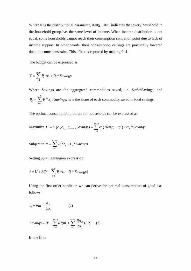
Where θ is the distributional parameter, 0<θ≤1. θ=1 indicates that every household in

the household group has the same level of income. When income distribution is not

equal, some households cannot reach their consumption saturation point due to lack of

income support. In other words, their consumption ceilings are practically lowered

due to income constraint. This effect is captured by making θ<1.

The budget can be expressed as:

1

* *n n

i i S

i

Y P c P Savings

Where Savings are the aggregated commodities saved, i.e. Si=δi*Savings, and

1

* / .n n

S i i

i

P P S Savings

δi is the share of each commodity saved in total savings.

The optimal consumption problem for households can be expressed as:

Maximize 2

1 2,

1

( , ... , ) (2 ) *n n

n n i i i i S

i

U U c c c Savings m c c Savings

Subject to 1

* *n n

i i S

i

Y P c P Savings

Setting up a Lagrangian expression:

1

( * * )n n

i i S

i

U Y P c P Savings

Using the first order condition we can derive the optimal consumption of good i as

follows:

2

Si i

i

c m

(2)

1 1

( ) /2

n n n ni S

i i S

i i i

PSavings Y Pm P

(3)

B. the firm

23

Since the firm’s investment decision has an impact on its production, we discuss the

firm’s investment first. There are different types of investment. Here we classify them

into three types. (1) Investment in production to increase the capacity of production.

This is the conventional investment, e.g. purchase of new machinery. (2) Investment

in production innovation to increase the efficiency or improve the technology of

production. (3) Investment in product innovation so as to create new types of

commodity.

Since both type-1 investment and type-2 investment have the same consequence of

increasing the firm’s output, they are lumped together labelled IQ, indicating

investment increasing quantity of commodity. Although type-1 investment tends to

increase the firm’s capital and type-2 investment tends to increase the firm’s

technology of production, for simplicity, it is assumed IQ will lead to an increase in

production technology. Type-3 investment is to increase the number of commodity

varieties, so it is labelled IN. Type-3 investment involves a very high chance of

innovation failure and brings little short-term benefit to the firm, so the firm prefers IQ

to IN.

Regrading IQ, it is assumed that the firm can identify consumption ceilings as well as

the impact of the distributional effect on consumption, so the firm’s decision on IQ is

to invest a proportion of the gap between the constrained consumption ceiling and the

current consumption. After IQ is decided, the firm is to consider IN. Due to the high

risk of IN, the firm invests only some of the available funds. As such, IQ and IN can be

expressed as follows:

1 1

( )n n n n

Q i i

i i

I m c

(4)

1 1

( ) * ( )n n n n

N Q i i

i i

I Saving I Saving m c

(5)

Where λ and η are parameters, 0≤ λ ≤1, 0≤ η ≤1. When η =1, the firm invests in

product innovation all money left over after investment in production. λ indicates the

firm’s propensity to invest. When λ=1, the firm invests the highest amount in

production to produce a maximum amount of goods which will be purchased by the

household.

24

The total investment I is the sum of IQ and IN and the investment demand for

commodity i is calculated by its share (βi) in the total investment demand I.

1 1

* (1 ) ( )n n n n

N Q i i

i i

I I I Saving m c

(6)

*i iI I (7)

Finally, the outcome of IQ and IN is an increase in technology level and in varieties of

commodity, respectively. Since the increase in technology and in types of new

products is assumed small, a log function is employed. Moreover, to reflect the high

chance of product innovation failure, a minimum investment amount (M) is used for

the outcome of investment in product innovation.

log

(log log )

i Q

N

A I

N PosiIntegral I M

Where PostiIntegral is a function which returns the largest positive integral contained

in the given value.

Regarding the firm’s production, the following Cobb-Douglas production function is

used for the purpose of simplicity:

1( )* *i i

i i i i ix A A L K

(8)

The optimal production problem can be expressed as:

Minimize * *L i K iCost P L P K

Subject to 1

( )* *i i

i i i i iOutput x A A L K

Setting up a Lagrangian expression:

1* * [ ( )* * ]i i

L i K i i i i i iP L P K x A A L K

Using the first order condition we can show optimal demand for labour and capital as

follows:

25

1

(1 )

i

i i Ki

i i i L

x PL

A A P

(9)

and

(1 )i

i i Li

i i i K

x PK

A A P

(10)

These results link the firm’s demand for labour and capital to the firm’s output xi.

More generally, the results show that the factor market is closely related to the

commodity market.

5. Results interpretation

Using the above model and the concept of excess demand (or excess supply), we can

discuss how and when an economic recession will occur, as well as its features. The

discussion here focuses on the commodity market and the factor market.

A. the commodity market

For an economy to grow without a recession, the condition for general equilibrium

must be satisfied, i.e. the total supply of commodity must be cleared by the market.

The total supply of a commodity can be categorized as either consumed or

unconsumed (saved), so the supply of commodity xi is the sum of both the consumed

and unconsumed commodity xi, namely, Si i ix c S . On the other hand, the demand

for commodity xi comprises the consumption demand and the investment demand, so

that the total demand for xi can be expressed as Di i ix c I . Thus, the excess demand

function for xi is: i Di Si i iED x x I S . Summing up the excess demand functions

for all commodities, we arrive at 1 1 1

n n n n n n

i i i

i i i

ED ED I S I Saving

.

This equation indicates that the equilibrium of the commodity market hinges on the

balance of saving and investment. If total investment demand is greater than total

savings, there will be overall excess demand for commodities in the economy. On the

other hand, if savings cannot be fully used for investment purposes, there will be an

26

overall excess supply of commodities. To achieve the market clearance and thus to

avoid an economic recession, the overall excess demand ED must be non-negative.

Recalling the investment equation (Equation 6), we can express the condition to avoid

a recession as:

1 1

1 1

[ * (1 ) ( )] 0

0

n n n n

i i

i i

n n n n

i i

i i

ED Saving m c Saving

or

m c Saving

Plugging the consumption equation (equation 2) and the saving equation (equation 3)

into the above inequality, we have:

1 1 1 1

( ) ( ) / 02 2

n n n n n n n nS i S

i i i i S

i i i ii i

Pm m Y Pm P

or

1 1 12 2

n n n n n nS S i S

i i

i i ii i

P PY Pm

(11)

This inequality shows that, to avoid a recession, the household income must be below

certain level! To increase the level of income, one may increase θ (i.e. improving the

equality in income distribution) or increase λ (the propensity to invest), but the effect

of these efforts is limited because the maximum value of both parameters is 1. The

only unrestricted way to increase income level is to increase ∆n, i.e. inventing new

products. Since θmi is much larger compared to αs/2αi, when ∆n increases, the

increase in the first term on the right hand side will outweigh the increase in the third

term and thus the cap on Y will be lifted. The question worth asking here is: why is

product innovation not fast enough to lift the cap on Y and thus to avoid a recession?

The key lies in the obstacles to innovation activities.

One such obstacle is the high risk of investment in innovation. Innovation by

definition involves the creation of something new. Inventors are continuously

stepping into uncharted territory, so it is understandable that many successful

27

innovations come only after numerous failed experiments. Although statistics on

innovation failure/success are difficult to obtain, it is widely accepted that a high

percentage of R&D investment is not successful. There are two types of innovations:

product innovation and production innovation. The goal of the former is to invent new

products while the effort of the latter is to improve production efficiency. Compared

with production innovations, product innovation has much higher risk of failure

because it normally involves much larger (or more radical) change and there is much

less information available to investors.

The other factor hindering innovation is imitation. Innovation requires hard and

intelligent work, takes a long time, and requires a great deal of money. Imitating an

innovation is, however, fairly easy. For example, software that takes several years and

costs millions of dollars to develop, may take only a few minutes to copy. Product

innovation is much more vulnerable to imitation than production innovation. Because

production innovations are applied to production procedures or machinery, imitating

these innovations requires knowledge about the production environment. Imitating a

new product does not, however, require this knowledge. The vulnerability of product

innovation to imitation means that the externality of product innovation is enormous.

Due to the distinct possibility of innovation failure and the low chance of getting a

good return because of imitation, risk-averse investors are reluctant to invest their

money in innovations, especially in product innovation. Rather, they prefer to invest

in production that has a relatively certain investment return. Therefore, innovation

investments, or R&D funds, become scarce, and this leads to scarcity of product

innovation activity.

The scarcity of production innovation leads to the fixed cap on Y and thus to the

economic stagnation. When the household tries to break the cap on Y by supply

supplying more labour and capital to the firm, the firm will produce more

commodities than can be cleared by the market. This will cause a recession. During an

economic recession or stagnation, it is not profitable to invest in production because

the goods are unsellable, so investors are forced to invest in product innovation in the

hope of obtaining a profitable new product. As such, ∆n increases, the cap on Y is

lifted, and the economy start to recover and expand. This recession-recovery-

expansion cycle will continue and result in cyclic economic growth.

28

Is there any way to stimulate investment in production innovation so as to avoid this

cyclic growth? Although no one can change the high-risk nature of product innovation,

one can balance this high risk with high return through forbidding imitation. An effort

of this kind is the IP laws, but the limitations in current IP laws lead to inappropriate

use of innovation rights from time to time. A full discussion of the limitations of IP

laws is covered by another paper, here we discuss only very briefly. On one hand,

current patent laws impose limited duration and a compulsory license rule on patent

rights, aiming at moderating the monopoly power of the patentee and at forcing the

patentee to implement patented technology. These clauses cause considerable stress

for inventors and discourage innovation. The maximum duration for a patent is about

20 years currently9, which limits the return to the patentee. The compulsory license

rule goes further. It stipulates that, 3 years after the date of the grant of the patent,

anyone can apply to the comptroller for a license under the patent. On the other hand,

the patent laws allow granting exclusive patent licenses, which transfer monopoly

power of patentees to licensees so that the patent monopoly power magnifies in the

economy. This aggravates the problem of abusing patent monopoly power.

A thorough revision of patent laws can further encourage innovation activity while

overcoming problem of patent monopoly power abuse in a positive way. For example,

abolishing the time constraint put on patentees, forbidding the assignment of patent

rights and exclusive patent licensing (to avoid the magnification of patent monopoly

power), and implementing a non-exclusive patent licensing system. Under this system,

anyone could use the innovation by applying for a license from the inventor.

Furthermore, the inventor would have a right to refuse licensing, but only on the

grounds of license price. With the product (the right of patent licensing) accurately

specified and the property right of patent licensing established and clearly defined

(infinite duration of patent right) in the new system, a patent market may come into

reality and it will automatically channel funds into innovation activities.

9 In some cases, it even prohibits the patentee from profiting from innovation. e.g. innovation in

medicine takes a long time and patentees are required by law to conduct animal and human trials before

making drugs publicly available.

29

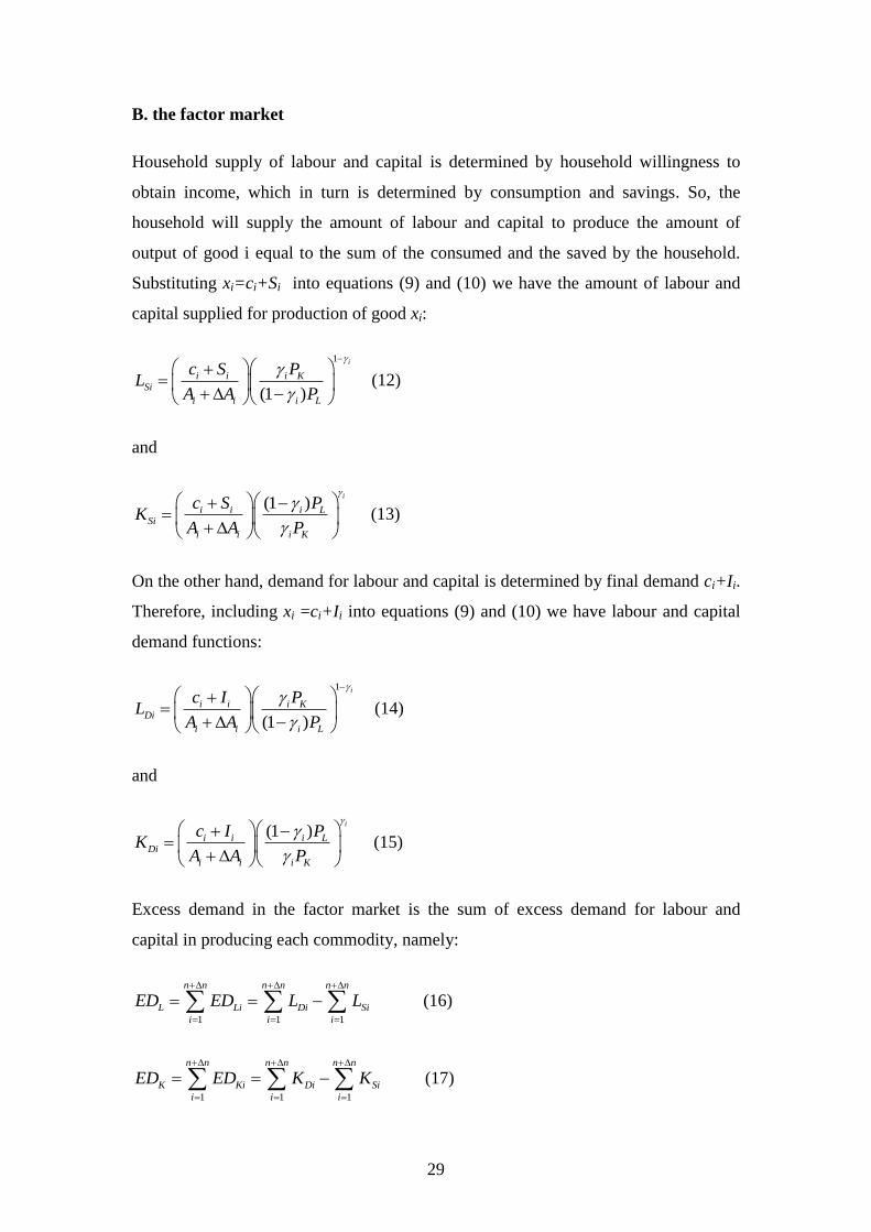
B. the factor market

Household supply of labour and capital is determined by household willingness to

obtain income, which in turn is determined by consumption and savings. So, the

household will supply the amount of labour and capital to produce the amount of

output of good i equal to the sum of the consumed and the saved by the household.

Substituting xi=ci+Si into equations (9) and (10) we have the amount of labour and

capital supplied for production of good xi:

1

(1 )

i

i i i KSi

i i i L

c S PL

A A P

(12)

and

(1 )i

i i i LSi

i i i K

c S PK

A A P

(13)

On the other hand, demand for labour and capital is determined by final demand ci+Ii.

Therefore, including xi =ci+Ii into equations (9) and (10) we have labour and capital

demand functions:

1

(1 )

i

i i i KDi

i i i L

c I PL

A A P

(14)

and

(1 )i

i i i LDi

i i i K

c I PK

A A P

(15)

Excess demand in the factor market is the sum of excess demand for labour and

capital in producing each commodity, namely:

1 1 1

n n n n n n

L Li Di Si

i i i

ED ED L L

(16)

1 1 1

n n n n n n

K Ki Di Si

i i i

ED ED K K

(17)

30

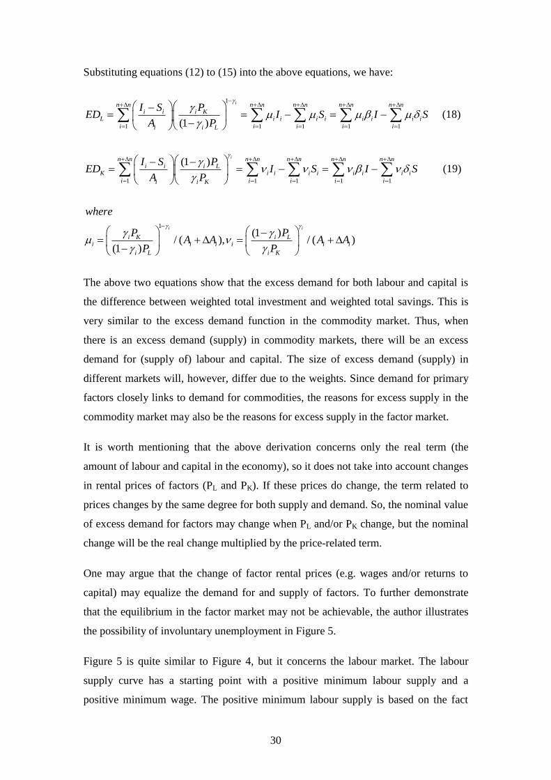
Substituting equations (12) to (15) into the above equations, we have:

1

1 1 1 1 1(1 )

in n n n n n n n n ni i i K

L i i i i i i i i

i i i i ii i L

I S PED I S I S

A P

(18)

1 1 1 1 1

(1 )in n n n n n n n n n

i i i LK i i i i i i i i

i i i i ii i K

I S PED I S I S

A P

(19)

1

(1 )/ ( ), / ( )

(1 )

i i

i K i Li i i i i i

i L i K

where

P PA A A A

P P

The above two equations show that the excess demand for both labour and capital is

the difference between weighted total investment and weighted total savings. This is

very similar to the excess demand function in the commodity market. Thus, when

there is an excess demand (supply) in commodity markets, there will be an excess

demand for (supply of) labour and capital. The size of excess demand (supply) in

different markets will, however, differ due to the weights. Since demand for primary

factors closely links to demand for commodities, the reasons for excess supply in the

commodity market may also be the reasons for excess supply in the factor market.

It is worth mentioning that the above derivation concerns only the real term (the

amount of labour and capital in the economy), so it does not take into account changes

in rental prices of factors (PL and PK). If these prices do change, the term related to

prices changes by the same degree for both supply and demand. So, the nominal value

of excess demand for factors may change when PL and/or PK change, but the nominal

change will be the real change multiplied by the price-related term.

One may argue that the change of factor rental prices (e.g. wages and/or returns to

capital) may equalize the demand for and supply of factors. To further demonstrate

that the equilibrium in the factor market may not be achievable, the author illustrates

the possibility of involuntary unemployment in Figure 5.

Figure 5 is quite similar to Figure 4, but it concerns the labour market. The labour

supply curve has a starting point with a positive minimum labour supply and a

positive minimum wage. The positive minimum labour supply is based on the fact

31

that people have to do a minimum amount of work to make a living (or at least keep

alive). The positive minimum wage is needed to reproduce labour. It is often argued

that unemployment in the economy is largely voluntary due to the wage floor imposed

by the Union or the government. While it is true that a wage floor (e.g. w1 or the

dotted line in Figure 5) can cause voluntary unemployment, Figure 6 also shows that

even if the wage floor is abolished, there is still a possibility of unemployment. When

the demand for labour decreases due to a decrease in investment demand (which is in

turn due to a lack of profitable opportunity), the labour demand curve pivots left from

DL to DL’. This leads to an equilibrium of labour supply and demand at a lower level

of employment and lower level of wages. There is no involuntary unemployment in

this case. However, as the labour demand curve pivots further from DL’ to DL’’ due

to a further decrease in investment demand, the labour demand curve cannot meet

with the labour supply curve and thus labour demand falls short of labour supply. This

will cause involuntary unemployment. Even the minimum wage can be approaching

zero (i.e. the starting point of SL approaches the point on the horizontal axis at L0),

there still exists involuntary unemployment because the labour demand can be less

than the minimum labour supply L0.

Figure 5. The possibility of involuntary unemployment

6. Conclusions

Based on observations and reasoning in the real world, this paper proposed three

axioms. (1) There is a consumption saturation point for each commodity per

household. (2) Savings can generate utility for households directly and immediately.

L

w

DL’’

SL

DL’

DL

L0

w1

32

(3) Investment demand is critically determined by profitability and, at the

macroeconomic level, the latter is indicated by growth of household consumption.

In including these axioms in a multi-commodity model, the paper explains economic

recessions around the world. An economic recession can be attributed to stagnation of

household consumption due to the existence of consumption saturation points and due

to the scarcity of product innovation. Using growth of household consumption as an

indicator of profitability, investors tend to increase investment when household

consumption increases, and decrease investment when household consumption

stagnates. Stagnation in both household consumption and investment demand will

drive the economy into a deep recession.

The paper also explains the cyclic economic growth and the vital role of product

innovation – the scarcity of product innovation underpins the cyclic growth pattern

and is a major obstacle to long-run economic development. The discussion on the

reasons for innovation scarcity and on the limitations in current IP laws points to the

necessity to revise the laws regarding intellectual property rights, the patent laws in

particular. Strong patent laws would lead to the formation of a functional patent

market. If the synergy of capital market and patent market can maintain an

appropriate balance between investment in product innovation and investment in

production, the pace of product innovation is balanced with the pace of production. As

a result, economic recessions can be avoided and faster and smoother rates of

economic growth can be achieved.

33

References:

Akerlof, G and Yellen, J. 1985, Can Small Deviations from Rationality Make Significant Differences to

Economic Equilibria? American Economic Review, 75(4): 708-720.

Cass, D., 1965, Optimum Growth in an Aggregative Model of Capital Accumulation, Review of

Economic Studies, 32: 233-240.

Davidson, P., 1984, Reviving Keynes’s Revolution, Journal of Post Keynesian Economics, Fall.

Davidson, P., 1991, Is Probability Theory Relevant for Uncertainty? A Post Keynesian Perspective,

Journal of economic perspectives, winter.

European Commission, 2013, Unemployment Statistics,

http://epp.eurostat.ec.europa.eu/statistics_explained/index.php?title=File:Unemployment_rate,_2001-

2012_%28%25%29.png&filetimestamp=20130627102805.

Fisher, I., 1930, The theory of Interest, New York: The Macmillan Co.

Fisk, E, 1962, Planning in a Primitive Economy: Special Problems of Papua New Guinea, Economic

Record, 38: 462-478.

Friedman, M., 1957, A Theory of the Consumption Function, Princeton University Press.

Howe, H, 1975, Development of the Extended Linear Expenditure System from Simple Saving

Assumptions, European Economic Review, 6: 305-310.

Keynes, J.M., 1936, The General Theory of Employment, Interest, and Money. London: MacMillan and

Co.

Koopmans, T., 1965, On the Concept of Optimal Economic Growth, in The Econometric Approach to

Development Planning, North Holland, Amsterdam.

Kydland, F.E. and Prescott, E.C., 1982, Time to Build and Aggregate Fluctuations, Econometrica, 51:

1345-1370

Lluch, C., 1973, The Extended Linear Expenditure System, European Economic Review, 4: 21-32.

Lucas, R.E., 1975, An Equilibrium Model of the Business Cycle, Journal of Political Economy,

December

Mankiw, N. G. , 1985, Small Menu Costs and Large Business Cycles: A Macroeconomic Model of

Monopoly, The Quarterly Journal of Economics , Vol. 100, No. 2 (May), pp. 529-537

Mankiw, N.G., 1989, Real Business Cycles: a New Keynesian Perspective, Journal of Economic

Perspectives, Summer

Modigliani, F., 1986, Life cycle, Individual Thrift, and the Wealth of Nations, American Economic

Review, 76: 297–313.

Modigliani, F., and Brumberg, R. 1954, Utility Analysis and the Consumption Function: An

Interpretation of Cross-section Data, in K. Kurihara ed., Post-Keynesian Economics,

Rutgers University Press, New Brunswick.

Pigou, A.C., 1943, The Classical Stationary State, Economic Journal, 53: 343-351.

Plosser, C.I., 1989, Understanding Real Business Cycles, Journal of Economic Perspectives, Summer.

34

Prescott, E.C., 1986, Theory Ahead of Business Cycle Measurement, Federal Reserve Bank of

Minneapolis Quarterly Review, Fall.

Ramsey F., 1928, A Mathematical Theory of Saving, Economic Journal, 38: 543-559.

Romer, D., 1993, the New Keynesian Synthesis, Journal of Economic Perspectives, winter.

Sorensen, P. and Whitta-Jacobsen, H., 2010, Introducing Advanced Macroeconomics (2nd ed),

McGraw-Hill, London.

Stent, W., and Webb, L., 1975, Subsistence Affluence and Market Economy in Papua New Guinea,

Economic Record, 51: 522-538.

Tobin, J. 1969, A General Equilibrium Approach to Monetary Theory, Journal of Money Credit and

Banking.

Witt, U., 2001, Escaping Satiation: the Demand Sside of Economic Growth, Springer.