Embed Size (px)
Citation preview
NBER WORKING PAPER SERIES
HOW THE GROWING GAP IN LIFE EXPECTANCY MAY AFFECT RETIREMENT BENEFITS AND REFORMS
Alan J. AuerbachKerwin K. CharlesCourtney C. Coile
William GaleDana Goldman
Ronald LeeCharles M. LucasPeter R. Orszag
Louise M. SheinerBryan TysingerDavid N. WeilJustin WolfersRebeca Wong
Working Paper 23329http://www.nber.org/papers/w23329
NATIONAL BUREAU OF ECONOMIC RESEARCH1050 Massachusetts Avenue
Cambridge, MA 02138April 2017
This paper draws on a report produced by the National Academies of Sciences’ Committee on the Long-Run Macroeconomic Effects of the Aging U.S. Population – Phase II, of which Lee and Orszag were co-chairs and the other authors were members (except Tysinger, on staff at the Roybal Center). The authors thank staff director Kevin Kinsella for his support of the committee’s work and staff at the Roybal Center for Health Policy Simulation, Leonard D. Schaeffer Center for Health Policy & Economics, University of Southern California for assistance with the Future Elderly Model simulations. The views expressed herein are those of the authors and do not necessarily reflect the views of the National Bureau of Economic Research.
At least one co-author has disclosed a financial relationship of potential relevance for this research. Further information is available online at http://www.nber.org/papers/w23329.ack
NBER working papers are circulated for discussion and comment purposes. They have not been peer-reviewed or been subject to the review by the NBER Board of Directors that accompanies official NBER publications.
© 2017 by Alan J. Auerbach, Kerwin K. Charles, Courtney C. Coile, William Gale, Dana Goldman, Ronald Lee, Charles M. Lucas, Peter R. Orszag, Louise M. Sheiner, Bryan Tysinger, David N. Weil, Justin Wolfers, and Rebeca Wong. All rights reserved. Short sections of text, not to exceed two paragraphs, may be quoted without explicit permission provided that full credit, including © notice, is given to the source.

How the Growing Gap in Life Expectancy May Affect Retirement Benefits and Reforms
Alan J. Auerbach, Kerwin K. Charles, Courtney C. Coile, William Gale, Dana Goldman, Ronald
Lee, Charles M. Lucas, Peter R. Orszag, Louise M. Sheiner, Bryan Tysinger, David N. Weil,
Justin Wolfers, and Rebeca Wong
NBER Working Paper No. 23329
April 2017
JEL No. H50,J10
ABSTRACT
Older Americans have experienced dramatic gains in life expectancy in recent decades, but an
emerging literature reveals that these gains are accumulating mostly to those at the top of the income
distribution. We explore how growing inequality in life expectancy affects lifetime benefits from
Social Security, Medicare, and other programs and how this phenomenon interacts with possible
program reforms. We first project that life expectancy at age 50 for males in the two highest
income quintiles will rise by 7 to 8 years between the 1930 and 1960 birth cohorts, but that the two
lowest income quintiles will experience little to no increase over that time period. This
divergence in life expectancy will cause the gap between average lifetime program benefits
received by men in the highest and lowest quintiles to widen by $130,000 (in $2009) over this
period. Finally we simulate the effect of Social Security reforms such as raising the normal
retirement age and changing the benefit formula to see whether they mitigate or enhance the
reduced progressivity resulting from the widening gap in life expectancy.
Alan J. Auerbach
Department of Economics
530 Evans Hall, #3880 University
of California, Berkeley Berkeley,
CA 94720-3880
and NBER
Kerwin K. Charles
Harris School of Public Policy
University of Chicago
1155 East 60th Street
Chicago, IL 60637
and NBER
Courtney C. Coile
Department of Economics
Wellesley College
106 Central Street
Wellesley, MA 02481
and NBER
William Gale
Brookings Institution
1775 Massachusetts Avenue, NW
Washington, DC 20036
Dana Goldman
Schaeffer Center for Health Policy and Economics
University of Southern California
635 Downey Way
Los Angeles, CA 90089-3333
Ronald Lee
Departments of Demography and Economics
University of California, Berkeley
2232 Piedmont Avenue
Berkeley, CA 94720
Charles M. Lucas
Osprey Point Consulting
Deer Isle, Maine 04627
Peter R. Orszag
Lazard
30 Rockefeller Plaza
New York, NY 10112
Louise M. Sheiner
Brookings Institution
1775 Massachusetts Avenue N.W.
Washington, DC 20036

Bryan Tysinger
Schaeffer Center for Health Policy
and Economics
University of Southern California
635 Downey Way
Los Angeles, CA 90089-3333
David N. Weil
Department of Economics
Box B
Brown University
Providence, RI 02912
and NBER
Justin Wolfers
Department of Economics
University of Michigan
611 Tappan St
Lorch Hall #319
Ann Arbor, MI 48104
Rebeca Wong
University of Texas Medical
Branch Sealy Center on Aging
301 University Blvd.
Galveston, TX 77555-0177

1
People with higher socioeconomic status have historically enjoyed longer life
expectancies than those with lower socioeconomic status. While this phenomenon has been
documented since the 1970s (Kitagawa and Hauser, 1973), researchers have only recently begun
to explore how the gap in life expectancy by socioeconomic status is evolving over time.
Although there are some inherent challenges in this work, the emerging consensus of this
nascent literature is that the gap is wide and has been increasing over time (Waldron, 2007;
Bound et al, 2014). Recent well-publicized studies by Case and Deaton (2015) and Chetty et al
(2016) have helped to bring this issue to the attention of the general public.
While the widening gap in life expectancy in the US is increasingly well documented,
its impact on government programs such as Social Security and Medicare has received far less
attention. Yet the implications for these programs are potentially quite substantial. These
programs provide benefits annually from the age of initial benefit claim, which occurs between
ages 62 and 70 for Social Security retired worker benefits and at age 65 (or earlier, in the case
of disability) for Medicare, until death. When life expectancy increases for those at the top of
the income distribution, they collect additional years of benefits. There is little corresponding
increase in taxes paid, except to the extent that having a longer life expectancy may induce
people to work longer. By contrast, if those at the bottom of the income distribution are not
experiencing a similar increase in life expectancy, there is no increase in their total lifetime
benefits. Thus the widening gap in life expectancy has the potential to greatly affect the
lifetime progressivity of entitlement programs as well as their long-term solvency.
A recent National Academies panel on which we participated explored the growing gap
in life expectancy by socioeconomic status and its implications for government entitlement
programs (Committee on the Long-Run Macroeconomic Effects of the Aging U.S. Population,

2
2015; hereafter, the Committee). In this paper, we build upon the Committee’s work and
expand on the implications of its findings for the US and other countries facing widening
inequality in life expectancy.
Our analysis proceeds in three steps. First, we project how life expectancy at older ages
is evolving over time by socioeconomic status. We use lifetime income quintile as our core
measure of socioeconomic status and estimate mortality models that allow for differential trends
by income quintile, using data from the Health and Retirement Study (HRS) linked to Social
Security earnings histories. From these models, we project survival after age 50 for the 1930
and 1960 cohorts, by income quintile. Next, we estimate the present value of lifetime benefits
by cohort and income quintile. We include benefits from Social Security, Disability Insurance,
Supplemental Security Income, Medicare, and Medicaid and look at benefits, benefits net of
taxes, and net benefits as a share of lifetime wealth. These projections are based on the Future
Elderly Model (FEM), a demographic and economic simulation model that uses data from the
HRS and other sources and has been employed to project trends in health care outcomes and
costs in studies such as Goldman et al (2005). Finally, we use the FEM to estimate the effect of
potential reforms to Social Security and Medicare. In each case, we simulate the reform’s effect
on lifetime benefits and discuss how this compares to and interacts with the changes in benefit
progressivity that are occurring due to changing life expectancy by income quintile. All of the
FEM simulations assume that Social Security and Medicare benefits will continue to be paid in
the future, even though the trust funds from which these benefits are projected to be exhausted
(see OASDI, 2016). Assuming that benefits will be paid as written under current law is the
approach used by the Congressional Budget Office in its long-term budget projections and
seems more in accordance with Congressional intent than assuming an abrupt cut in benefits in

3
the future when the trust funds run out.
Our paper offers a number of contributions relative to the previous literature. First, we
summarize the complex methodological issues involved in projecting life expectancy by
socioeconomic status and provide new estimates to complement those in other studies.1
Second, we assess the progressivity of government benefits and how this is changing over time
due to the widening gap in life expectancy by socioeconomic status. While there are studies
that explore the progressivity of individual programs such as Social Security or Medicare (e.g.,
Liebman, 2002; Bhattacharya and Lakdawalla, 2006), this is the first study of which we are
aware that estimates the progressivity of government benefits for the older U.S. population
(those aged 50 and above) as a whole. Moreover, the previous literature has tended to look at
progressivity at a point in time, rather than how it evolves over time with a widening gap in life
expectancy, which is the primary focus of this study. Finally, there are relatively few studies
that focus on the distributional effects of possible reforms to Social Security or other
government programs (Gustman and Steinmeier, 2014 and Coronado et al, 2002 are examples),
and those few do not focus on how this might be changing over time with the growing gap in
life expectancy.
We have several major findings. First, consistent with other recent studies, we confirm
that life expectancy at older ages has been rising fastest for the highest socioeconomic
groups. For those born in 1930, the gap in life expectancy at age 50 between males in the
bottom 20 percent and top 20 percent of lifetime income is 5 years, according to our estimates.
For males born 30 years later (in 1960), the projected gap at age 50 between the highest and
lowest quintiles widens to almost 13 years, an increase of nearly 8 years. Second, we find that
1 Bound et al. (2015) also discuss some of these methodological issues.

4
there is a growing gap by lifetime income in projected lifetime benefits from programs such as
Social Security and Medicare. For the 1930 cohort, the present value of lifetime benefits at age
50 is roughly equal for those in the highest and lowest quintile of lifetime income, as those at
the top receive more from Social Security while those at the bottom receive more from
Disability Insurance, Supplemental Security Income, and Medicaid. For the 1960 cohort, by
contrast, there is a $130,000 gap in benefits between the highest and lowest quintiles, as those
in the top quintile are increasingly likely to receive benefits over longer periods of time,
relative to those at the bottom. Finally, we show that a number of commonly-discussed Social
Security reforms would make the program more progressive, although their impact on
progressivity tends to be small compared to the changes arising due to differential changes in
life expectancy.2
I. Background on Socioeconomic Status and Mortality
For the US, research on differences in mortality by socioeconomic status (SES) has a
long history, including the landmark study by Kitagawa and Hauser (1973) that found important
differences in 1969 mortality by educational attainment. Differences in the mortality of African
Americans and Whites also have been documented throughout the 20th century, with a gap of 7.1
years in 1993. That gap has declined since then, to 3.4 years in 2014. Given this, one might have
expected that SES differences had narrowed in general, but the opposite is the case. Study after
study has found that SES differences have been widening in recent decades, whether SES is
measured by educational attainment or by income. Before reviewing these studies, we will
briefly consider some of the methodological difficulties in this area. 2 Here and elsewhere in the paper, we use the term “progressive” as it is traditionally defined in economics (e.g., that a tax (benefit) is progressive if the average tax (benefit) rate rises (falls) with income) and not as it is sometimes used in political discussions in the U.S. (e.g., as a synonym for liberal).

5
Methodological Issues
One of the biggest problems is reverse causality: while differences in SES may lead to
differences in health and survival through various routes, it is also true that differences in health
may lead to differences in income by affecting the ability of adults to work, by incurring out of
pocket health care costs, and perhaps by affecting the educational attainment of children early in
life and thereby earnings throughout life (Smith, 2004, 2007). Education-based measures of SES
are at less risk in this regard than income based measures, because unlike income, education is
largely fixed early in life. For our purposes here, reverse causality is not necessarily an issue,
because if ill health causes both lower income and shorter life the consequence is nonetheless
that the lower income person in question receives government old age benefits over fewer years.
The one possibility that we do need to exclude is that a short-term illness causes both a short-
term decline in income and a higher risk of death, because this association of short term changes
will exaggerate the implications for receipt of government benefits over the longer term. Use of a
long-term measure of income, as will be discussed later, greatly reduces this problem,
particularly if it describes incomes earlier in life relative to the survival outcome.
When the analysis period spans many years, there is a different problem: the meaning of
an inflation-adjusted dollar of income changes over time, and relative position in the income
distribution of each year or generation may be a more meaningful measure. For this reason, the
standard approach has been to use income quantiles, rather than absolute income, as the SES
measure.
While measuring SES by educational attainment reduces the problem of reverse
causality, it brings a new problem: increasing adverse selection for those in low attainment
categories such as less than high school graduation, as the general level of attainment in the
6
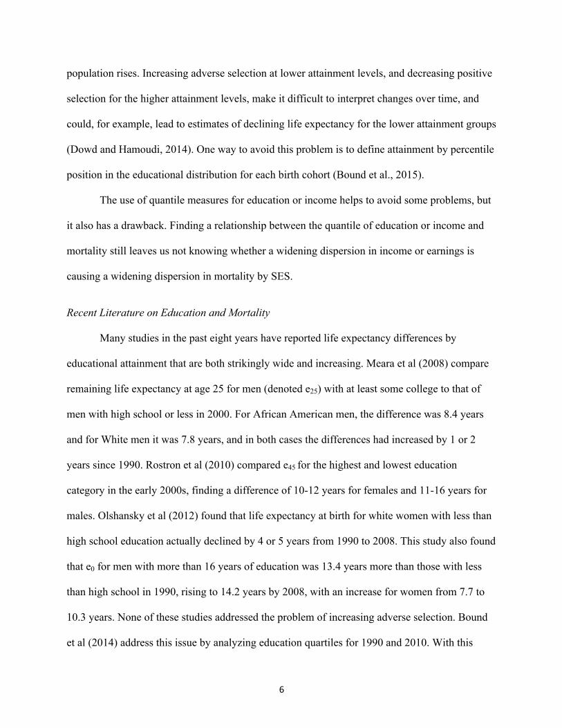
population rises. Increasing adverse selection at lower attainment levels, and decreasing positive
selection for the higher attainment levels, make it difficult to interpret changes over time, and
could, for example, lead to estimates of declining life expectancy for the lower attainment groups
(Dowd and Hamoudi, 2014). One way to avoid this problem is to define attainment by percentile
position in the educational distribution for each birth cohort (Bound et al., 2015).
The use of quantile measures for education or income helps to avoid some problems, but
it also has a drawback. Finding a relationship between the quantile of education or income and
mortality still leaves us not knowing whether a widening dispersion in income or earnings is
causing a widening dispersion in mortality by SES.
Recent Literature on Education and Mortality
Many studies in the past eight years have reported life expectancy differences by
educational attainment that are both strikingly wide and increasing. Meara et al (2008) compare
remaining life expectancy at age 25 for men (denoted e25) with at least some college to that of
men with high school or less in 2000. For African American men, the difference was 8.4 years
and for White men it was 7.8 years, and in both cases the differences had increased by 1 or 2
years since 1990. Rostron et al (2010) compared e45 for the highest and lowest education
category in the early 2000s, finding a difference of 10-12 years for females and 11-16 years for
males. Olshansky et al (2012) found that life expectancy at birth for white women with less than
high school education actually declined by 4 or 5 years from 1990 to 2008. This study also found
that e0 for men with more than 16 years of education was 13.4 years more than those with less
than high school in 1990, rising to 14.2 years by 2008, with an increase for women from 7.7 to
10.3 years. None of these studies addressed the problem of increasing adverse selection. Bound
et al (2014) address this issue by analyzing education quartiles for 1990 and 2010. With this

7
approach they find no decline in life expectancy for low education women, but they do find a
difference of 6-7 years in the median age at death in 2010 between the bottom quartile of males
and the top three quartiles, and this difference had roughly doubled since 1990. Hendi (2015)
also explicitly addresses the selection problem using different methods. This study finds a
difference in e25 between less than high school and college of about ten years for both White men
and women, and finds that the difference is growing. It also finds that e25 declined for least-
educated White women, with only some of the measured decline accounted for by selection. A
study by Goldring et al (2015) reported no evidence that mortality declines were numerically
greater for high education men than for low, but they did not consider whether proportional
declines may have been greater for them, so it is not clear whether their findings are inconsistent
with the other studies. Case and Deaton (2015) found a significant increase between 1999 and
2013 in all-cause mortality of middle-aged non-Hispanics, with more dramatic increases for
those with less education and for whites. They suggest a potential connection with the opioid
epidemic and more broadly with economic distress. Overall, the findings of the studies using
educational measures are very consistent in showing very large and widening differences.
Recent Literature on Income and Mortality
A seminal study by Waldron (2007) based on mortality and earnings data from Social
Security and Medicare engendered a wave of closely related studies using a similar design based
on the Health and Retirement Survey (HRS) linked to Social Security earnings histories.
Waldron measured income as the average of non-zero Social Security earnings at ages 45 to 55.
It was not possible to use full lifetime earnings because many workers joined Social Security
later in their careers when coverage was expanding. For those reporting zero earnings in a year, it

8
was not possible to distinguish between those with no earnings and those whose earnings were
not covered by Social Security. Waldron related quantiles of this earnings measure to mortality
observed in later years in the age range 60 to 89 in the years 1972 to 2001, with ages depending
on the birth cohort.3 She projected future mortality for each birth cohort in order to get a measure
of e65. A striking chart shows that for the birth cohort of 1913, there was only a half-year
difference in e65 between the top half of the earnings distribution and the bottom half. For the
cohort born 28 years later in 1941, however, this difference had grown to 4.6 years, and while e65
for the bottom half of the earnings distribution rose by only a bit over one year, for the top half it
rose by about 6 years.
While Social Security data covers a huge population and has rich earnings histories, it
also has very few covariates. Bosworth and Burke (2014), building on Waldron’s studies, chose
to use the Health and Retirement Survey (HRS). Its sample is relatively small, but it is linked to
the Social Security earnings histories and it has exceptionally rich information on health,
disability, assets, pensions, and many other variables of potential interest. Bosworth and Burke
measure income as quantiles of the average of non-zero earnings for ages 41-50, and relate this
to mortality above age 50. For couples, they allocate to each the sum of their individual incomes
divided by the square root of two, to adjust for economies of scale in household consumption. A
later study by Bosworth, Burtless and Zhang (2016) uses a similar design but analyzes data from
both HRS (through the 2012 wave) and SIPP (Survey of Income and Program Participation). The
results are quite similar to Waldron. There is a difference in e50 between the highest and the
lowest earnings decile of 9 to 12 years for males and females born in 1940, a big increase
relative to the difference for the birth cohort of 1920.
Chetty et al. (2016) use tax data to study the gradient in life expectancy in different 3 Fewer and fewer years are observed for the more recent cohorts, ending in only one year for the 1941 birth cohort.

9
geographies. The results suggest not only a growing gradient by income, but that the
magnitude of the gradient is smaller in more affluent, more educated areas than in less
affluent, less educated ones.
One recent exception to the growing body of literature showing expanded life
expectancy gaps is Currie and Schwandt (2016), who find that low-income counties have
narrowed the gap in life expectancy at birth (but not at age 50) with high-income countries.
An important research agenda involves reconciling the results for children with those for
adults, including by examining differences in childhood mortality at the individual rather than
county level. In general, however, the literature points to substantial increases in life
expectancy differentials for adults.
II. Background on the Progressivity of Government Programs
Conceptual Issues
The growing gap in life expectancy by SES forces society to grapple with a key question
– is it “fair” for groups that experience larger gains in life expectancy to receive larger gains in
the present value of government benefits? For most government programs, policy makers do not
focus on lifetime benefits because there is no obvious time dimension: in any given year, people
who are alive pay taxes and receive benefits such as national defense and clean air. But for
programs where the ages at which taxes are paid and benefits received differ significantly, this
issue becomes critical. For brevity, we discuss this issue in terms of Social Security only,
although similar arguments may apply to Medicare and other programs.4
With Social Security, two concepts dominate discussions regarding fairness. The first is
4 Here and elsewhere in the paper, we use the term “Social Security” to refer to old-age benefits (OASI), rather than as an inclusive term that also includes Disability Insurance.

10
the expected rate of return on payroll tax contributions. In a system with an actuarially fair rate
of return, the present value of real benefits received is equal to the present value of real
contributions. In the US, early cohorts received more than fair average rates of return due to the
transfers inherent in starting a pay-as-you-go system; current and future cohorts receive less than
fair returns because of the costs of these transfers (Leimer, 1995). Of greater relevance here is
whether the average rates of return for different SES groups within a cohort are similar. Similar
rates of return across groups may align with basic notions of fairness, enhance political support
for the system, and minimize work disincentives. As the gap in life expectancy grows, the
average rate of return for the high SES group increases because longer life does not much
increase tax payments by members of the group but it does raise their years of benefits. If
societal notions of fairness dictate that all groups should receive an equal rate of return, then the
effects of the growing gap in life expectancy on the distribution of lifetime benefits are
undesirable.
The second key consideration for society is the extent to which Social Security should
redistribute from those with high lifetime earnings to those with low lifetime earnings. Any such
action naturally tends to make the rates of return unequal across groups, but may nonetheless be
desired by society, motivated by a utilitarian concern for the poorest members of society. While
the growing gap in life expectancy does not reduce the absolute benefits received by low-SES
groups (unless their life expectancy is declining), it does render the system relatively less
generous to such groups; moreover, it may threaten absolute benefits of low-SES groups by
straining the program’s finances. In practice, the US system seems to embrace both the rate of
return framing of Social Security (by referring to payroll taxes as contributions and tracking each
worker’s contributions over his or her life) and its redistributive role (by employing a progressive

11
benefit formula, as discussed below).
Another salient feature of Social Security is that it is an annuity. Such a system
necessarily redistributes from the short-lived to the long-lived, generating ex post inequality in
the rate of return. This may be contrasted with the ex ante inequality that would arise, for
example, if one group paid more in taxes but received the same benefit amount as another. Ex
post inequality does not offend notions of fairness because it is unpredictable – some 60-year-
olds live a long time, some do not – and the fact that the system provides larger lifetime benefits
to those who live longer is what it is designed to do, in order to insure against the risk of having a
long life and many years of consumption to finance. This may become problematic, however, if
there are identifiable groups that vary in life expectancy, as this introduces a non-random aspect
to the inequality.
Background on Government Programs
While a discussion of the institutional features of all major entitlement programs with
beneficiaries age 50 and above is impractical, we provide a few details that are most salient for
the programs’ distributional impact. We focus on Social Security, since most reform proposals
we later consider concern it.
Individuals are eligible for Social Security if they have 40 quarters of covered earnings.
To calculate benefits, past earnings are multiplied by a wage index and an average of the top 35
years of indexed earnings is calculated (Average Indexed Monthly Earnings, or AIME). A
piecewise linear formula is applied to the AIME to create the Primary Insurance Amount (PIA),
the basis for the monthly benefit. The formula introduces progressivity because the rate at which
AIME is translated into PIA declines as AIME increases. In 2016, each dollar of AIME up to the

12
first bend point of $856 is converted into 90 cents of PIA; the conversion factor is 32 percent
until the next bend point of $5,157 and 15 percent for earnings beyond this value.
The monthly benefit depends on the age at initial benefit claim. Workers may claim as
early as 62, the Early Eligibility Age (EEA), and as late as 70. Workers receive the PIA if they
claim at the Normal Retirement Age (NRA), which has been rising over time from age 65 (for
those born by 1937) to 67 (for those born in or after 1960). Workers face an actuarial reduction
(increase) for claiming before (after) the NRA, designed to ensure that the expected benefits
received over a worker’s lifetime are roughly the same regardless of claiming age.5 6 Dependent
and surviving spouses and children of insured workers are eligible for benefits; individuals who
are dually entitled receive the larger of the benefits to which they are entitled.
The Disability Insurance (DI) program is integrated with Social Security and its benefit is
similar, except there is no reduction for early claiming; eligibility requires passing a medical
screening and meeting recent work requirements. When DI recipients reach the NRA, they move
to Social Security. Social Security and DI benefits are funded by payroll taxes of 6.2 percent of
earnings by both employers and employees, up to a taxable maximum of $118,500 in 2016. The
Supplemental Security (SSI) program provides cash benefits to low-income individuals who are
age 65 and up, or who are blind or disabled. Benefits are $733 for a single person and $1,100 for
a couple but are reduced dollar-for-dollar against other benefits and income.
5 A workers whose NRA is 67 receives 70% of the PIA if he claims at age 62 and 124% of the PIA if he claims at age 70. Whether the reduction factor is, in fact, actuarially fair for a typical worker is a matter of some dispute. Shoven and Slavov (2013) argue that the gains from delaying Social Security have increased dramatically since the 1990s due to a combination of low interest rates, increasing longevity, and legislated increases in the gain for claiming delays beyond the NRA (the “Delayed Retirement Credit”). 6 A further complication in the benefit calculation is the Social Security earnings test. Before the NRA, workers face a reduction in benefits if they earn above an exempt amount ($15,720 in 2016). However, upon reaching the NRA, the worker is credited for any lost months of benefits through a recomputation of the actuarial adjustment. Although there is some evidence the earnings test may affect claiming behavior (Gruber and Orszag, 2003), it does not affect the (ex ante) progressivity of Social Security, and so we abstract from it in our discussion.

13
Medicare is available at age 65. Individuals are eligible if they or a spouse has worked
40 quarters. Medicare includes hospital insurance (part A) as well as optional supplemental
insurance that pays for physician services and prescription drugs (parts B, C, and D). Part A is
financed by payroll taxes on earnings, while other parts are financed by premiums and (mostly)
general revenues. Medicaid provides health insurance to low-income individuals; it is the
primary payer of long-term care services, which are not generally covered by Medicare. 7
Recent Literature on Progressivity
Estimating the progressivity of Social Security and other programs raises new challenges,
starting with how to measure it. One option is to compare the replacement rate (ratio of benefits
to average earnings) at different points in the income distribution.8 The OASDI Trustees (2013)
find the replacement rate for a worker is 42% for an average-wage worker, 56% for a low-wage
worker, and 35% for a high-wage worker. Naturally, the benefit amount rises with past earnings,
even though the replacement rate falls. By this measure, Social Security is highly progressive.
The replacement rate excludes contributions, however, yielding an incomplete picture of
progressivity.9 Some alternatives that address this (Geanakoplos et al, 1999) include the internal
rate of return (IRR; the rate at which an individual must be willing to trade off between present
and future income in order for the present value of benefits and taxes to be equal), benefit/tax
7 As this brief summary makes clear, the programs we incorporate in our analysis include self-financed programs (Social Security and DI), programs financed out of general revenues (SSI and Medicaid), and a program whose financing is a hybrid of the two (Medicare) 8 While it is typical to use career earnings, some use final earnings or an average of earnings in the years just before retirement; Goss et. al. (2014) compare replacement rates using alternative earnings measures. 9 Economic theory suggests that the incidence of employer contributions to Social Security may fall on workers, in the form of reduced wages; evidence from Gruber (1997) supports this hypothesis, and virtually all analysts adopt this convention in their calculations.

14
ratio (ratio of these present values, calculated at the market rate of discount), and the net transfer
(difference of these present values). As before, one can compare these measures at different
points in the income distribution. Liebman (2002) finds that the IRR is much higher for low-
income workers.
The results from any analysis of progressivity depend, to some extent, on decisions the
researcher must make in order to carry out the calculations, including the earnings measure used
to determine an individual’s place in the income distribution. Gustman and Steinmeier (2001)
and Coronado et. al (2011) find that the progressivity of Social Security is reduced or eliminated
when using lifetime rather than annual earnings, household rather than individual earnings, and
potential (with full-time work at the current hourly wage) rather than actual earnings.10
Another factor that is of particular interest here is differential mortality. As discussed
earlier, large and growing differences in mortality by SES are expected to reduce progressivity.
Liebman (2002) shows that when using mortality probabilities that vary only by age and sex, low
SES groups gain more from Social Security than do high SES groups (as measured using the IRR
or net benefits); however, when race- and education-specific mortality tables are used, the
progressive effect of the non-linear benefit formula is considerably smaller, due to the shorter
life expectancy of low-SES groups.
Turning to other programs, DI benefits are even more progressive than Social Security
because low-income workers are more likely to go on DI. A CBO analysis (2006) finds much of
the progressivity of the overall OASDI system is due to DI benefits. Analyses of Medicare
progressivity come to differing conclusions – Bhattacharya and Lakdawalla (2006) find that
10 These changes reduce progressivity because there may be people who have low earnings by the initial earnings measure and receive high net transfers who would be reclassified as higher earners under the new definition, such as a part-time worker (higher potential than actual earnings) or non-working spouse (higher household than individual earnings). Progressivity also falls when including earnings above the taxable maximum or using a higher discount rate (Fullerton and Mast, 2005) or using only workers who survive to age 62 in the analysis (CBO, 2006).

15
Medicare Part A expenditures are much larger for the less educated, while McClellan and
Skinner (2006) find total Medicare expenditures to be roughly similar by zip code income level.
Medicaid expenditures are unsurprisingly skewed towards low-SES groups, though De Nardi et
al (2013) find that use of Medicaid by high-income groups rises markedly with age, as
individuals spend down their assets and become eligible. Missing from all of these analyses is
an analysis of how much people value the benefits they receive. This is particularly important
for programs like Medicare and Medicaid that provide in-kind benefits rather than cash, because
it is unclear whether people value health spending at its cost. But all these programs offer more
than cash—because they are annuities, they also offer longevity insurance—the value of which
might vary across income groups.
III. Empirical Methods
We now turn to discussing our own projections of the gap in life expectancy by SES and
the progressivity of Social Security and other government programs. We begin with our
definition of lifetime income, a measure that is based on household earnings. In the work of the
Committee (2015) that we discuss here, we follow the approach of Bosworth and Burke (2014)
in using waves of the HRS from 1992 to 2008, covering cohorts born 1912 to 1957 (with
different years of coverage by cohort), and calculating mid-career earnings as the average of
annual earnings over ages 41 to 50, using those years with positive earnings only.11 For HRS
respondents for whom Social Security earnings records are unavailable or incomplete, we
11 Including years with zero earnings in the calculation of average earnings does not change the assignment to income quintile for the vast majority (over 85%) of the sample, suggesting that our key results are likely robust to this assumption.

16
impute earnings based on regressions.12 Earnings above the taxable cap were estimated based on
the month in which the cap was reached. Individual members of couples were assigned lifetime
income values equal to the sum of their individual mid-career earnings divided by the square root
of 2, an adjustment commonly made to reflect the fact that the living expenses of a two-person
household are somewhat greater than those for a one-person household, so a larger household
would need a larger income to be as well off in consumption terms.13 Finally, individuals are
assigned to a lifetime income quintile based on this value.
For our mortality model, we estimate probit equations where the dependent variable is the
death over a two-year period (between waves of the HRS). Our key regressors include a linear
time trend to capture the general improvement of health and mortality, the income quintile, and a
quintile specific time trend to capture changes in mortality dispersion. We did not include other
available covariates such as education or race/ethnicity, because to do so would work at cross-
purposes of the goal of our study. For our purposes it does not matter whether such variables are
associated with differences in health and mortality, as they surely are; even if these associations
accounted for all the difference in mortality, it would still be true that lower income people have
shorter lives and receive government benefits for fewer years in old age. For similar reasons we
do not include biomarkers or measures of health status as covariates. We carried out a number of
robustness and sensitivity checks with alternative model specifications. 12 We have complete earnings data for 68% of our sample. For the 5% of our sample that was born before 1910, we lack complete data on earnings at ages 41-50, since the Social Security Administration only began recording annual earnings in 1951. An additional 27% of our sample did not give the HRS permission to use their Social Security earnings records. 13 When we assign quintiles without making this adjustment, we find that people remain in the same quintile 89% of the time and move by more than one quintile in less than 0.5% of cases. Based on this, we conclude that our results are unlikely to be sensitive to this assumption. In addition, while we acknowledge that there might be other people in the household (e.g., children) and that one might theoretically wish to make an adjustment for this as well, we do not do so due to the difficulty of properly incorporating financial support to children in college in any such adjustment. We implicitly view the couple (or individual, for a single person) as the unit whose consumption needs will have to be supported in the long term and thus is most relevant for the analysis.

17
In this analysis, we estimate models and show results for men only. In Committee
(2015), we estimate gender-specific mortality models and present results for both men and
women. Unfortunately, the estimates for women appear to be less reliable than those for men.
For example, the results point to a continued narrowing of the male-female life expectancy gap
in the future, which is plausible, but also suggest that male life expectancy will be higher than
female, an outcome that is not consistent with projections by the Social Security Administration.
Estimates of mortality differences by income for females are often unstable or present other
problems (Waldron, 2007; Bosworth and Burke, 2014) and analysts typically focus on results for
men. We follow the literature in doing so, but direct interested readers to Committee (2015).
For our analysis of progressivity, we make use of the Future Elderly Model (FEM), a
demographic and economic simulation model designed to predict the future costs and health of
the older population and to estimate how this could be affected by health trends or policy
reforms.14 The FEM begins with a cohort of Americans at age 50 drawn from the HRS data.
Each individual in the cohort has a measure of lifetime income (measured as described above)
and an initial health status. The FEM features models that relate characteristics like age, income,
and health status to the probability of transitioning into various health and financial states,
including retirement, Social Security claiming, DI claiming, disease, and death. These models
are inherently associative rather than causal, although exogenous variation that occurs during the
sample period can help to identify model parameters – for example, individuals in the HRS face
different NRAs, which helps to identify the effect of being exactly at versus younger than the
NRA on the probability of transitioning to Social Security receipt. While the HRS (1992-2008
waves) is the primary data source for the FEM, information from the 2002-2004 Medicare
14 More details about the FEM model and these calculations are available at www.nap.edu/GrowingGap under the resources tab.

18
Current Beneficiary Survey (MCBS) and 2002-2004 Medical Expenditure Panel Survey (MEPS)
is used for estimating health expenditures. The estimates from the transition models are
combined with individual characteristics to estimate the probability that individuals will
transition across the various health and financial states over a two-year period. Using updated
characteristics, the model predicts transitions over the next period, and this process is repeated
until everyone in the cohort has died.
The baseline scenario is based on the initial health status distribution of the 1930 cohort
and its estimated mortality gradient. We then modify the initial health status distribution and
mortality gradient to that of the (simulated/projected) 1960 cohort and contrast the new results to
the baseline. Health status does not enter directly into the mortality or medical spending
equations, hence these outcomes are driven entirely by the mortality gradient. Health does
influence some economic outcomes, thus the differences in initial health prevalence will lead to
some cohort differences in trajectories after age 50 in earnings, labor force participation, and
claiming of Social Security, DI, and SSI, although the two cohorts have the same earnings up to
age 50 by construction. We also use the 2010 policy environment for both calculations, to
isolate the effect of changing mortality gradient alone. As a final step, we modify the policy
environment and simulate new results to contrast to the baseline, in order to show the effect of
the reforms on lifetime benefits.
We report our results in terms of three related outcome measures: the present value of
benefits at age 50 (expected benefits received after age 50, discounted back to that age using a
real rate of 2.9 percent), the present value of net benefits (same but net of all taxes paid after age
50), and the present value of net benefits as a share of inclusive wealth (net benefits relative to a
measure that includes asset holdings at age 50, after-tax earnings after age 50, and net benefits

19
after age 50, all in present value at age 50). We measure benefits received and taxes paid after
age 50, as opposed to on a full lifetime basis, because the FEM starts with a cohort of 50-year-
olds drawn from the HRS. Our measure of benefits should be quite similar to a lifetime measure,
since most benefits from Social Security, Medicare, and the other programs are received after
age 50, although our net benefit measure will overstate the extent of net transfers from the
government because it excludes taxes paid before age 50. However, the focus of our study is on
the change in gross and net benefits resulting from mortality changes after age 50, which is
unaffected by the exclusion of taxes earlier in life.
IV. Results
Mortality Projections
Later we will report the results of simulation experiments that isolate the effect of the
widening mortality dispersion on the lifetime value of government benefits received after age 50.
These simulations contrast these values under the mortality regimes of the birth cohort of 1930
and 1960. For this reason we will present our results for these two birth cohorts. However, it is
important to keep in mind that we do not actually observe even one year of deaths at age 50 or
above for the 1960 birth cohort, because it turns age 50 in 2010 and the latest wave of the HRS
that we use is 2008. Thus the mortality results for this birth cohort are slightly out-of-sample
estimates based on the fitted model. For the 1930 birth cohort, turning 50 in 1980, we have
observations or within sample simulations from age 62 in 1992 to age 78 in 2008. To estimate e50
we must extrapolate mortality to older ages until the cohort has died out, and this we do by
assuming that the trends estimated in the model continue, including the quintile divergence. The
quintile divergence applies to birth cohorts, not periods, so the amount of extrapolation is modest

20
– from cohorts born up to 1950 or so to the cohort of 1960. There is a further assumption, built
into the model specification, that a cohort’s income quintile has an age-dependent effect on its
mortality over the rest of its lifetime. Because some may find these assumptions too strong, the
Committee also calculated the implications of a trend in dispersion that was only half this large,
finding a convenient proportionality that permits the reader to consider other scenarios.
While the Committee’s analysis of mortality differentials was cohort based and
longitudinal, like those of Bosworth et al (2016) and Waldron (2007), there have been a number
of careful cross-sectional studies that have found continuing widening of the differentials up to
the present (e.g. Chetty et al, 2016; Currie and Schwandt, 2016, above age 50), and we are aware
of no studies indicating a recent narrowing of differentials or a slow down in their widening.
The trends and projections for overall life expectancy arrived at in this way are quite
similar to those in the Social Security Administration projections, which were also used by
Waldron (2007) for this purpose. But because those Social Security projections assume some
deceleration of mortality decline as time passes, the Committee’s projections of e50, which do
not, are slightly higher.
There is some evidence that the upward trend in US life expectancy has slowed in the last
few years. Ma et al (2015) report that declines in overall mortality and mortality due to various
causes of death slowed from 2010 through 2013 relative to earlier years. Consistent with this
finding, Xu et al (2016) report that US life expectancy declined by 0.1 years from 2014 to 2015,
primarily due to rising mortality for non-Hispanic white males and females and black males. Life
expectancy declines of this sort have occurred 12 times for US females since 1933 and 14 times
for males15. Whether this slowdown in mortality decline persists or proves transitory would not
in itself matter much for our main results which depend on the inter-quintile differences much 15 Thanks to Josh Goldstein for this observation (personal communication).

21
more than on the average level.
Our estimates of remaining life expectancy at age 50 by income quintile are shown in
Figure 1. Life expectancy at 50 is a convenient summary measure, but for our simulations we of
course used the survival probabilities to each age, which are not shown here. For the male birth
cohort of 1930, e50 is lowest for the bottom quintile and rises steadily as we move to higher
quintiles, reaching a level 5.1 years higher for the top quintile. For the 1960 male birth cohort the
lowest quintile has slightly lower e50 than the 1930 cohort, but then rises to a level 12.7 years
higher for the top quintile, indicating a very large increase in the dispersion.
There are, of course, many sources of uncertainty in our estimates of mortality
differences by income quintile, and even more so in the growth in these differences between the
cohorts of 1930 and 1960. While we were not able to assess this uncertainty formally, we did
also prepare mortality projections for the 1960 cohort on the assumption that the dispersion
increased only half as rapidly as in our baseline projection shown in Figure 1, as mentioned
earlier. We also carried out simulation experiments based on these alternative projections.
Progressivity of Lifetime Benefits
Next, we discuss our findings with respect to the progressivity of lifetime benefits from
government programs, contrasting the experience under the mortality conditions of the 1930 and
1960 cohorts. Recall that this exercise is not meant to obtain a projection of actual benefits for
these two cohorts, but rather to isolate the effect of the changing mortality gradient and initial
health distribution on lifetime benefits. In our simulation experiments the policy environment
and earnings up to age 50 are the same for both cohorts, though the actual two birth cohorts had
different experiences. Results are reported in 2009 dollars.

22
We begin with Social Security, reporting results in Figure 2. For males in the 1930
cohort, benefits rise with income quintile – workers in the lowest quintile can expect to receive,
on average, $126,000 of benefits over the rest of their lives (discounted to age 50), while workers
in the top quintile can expect to receive $229,000, or 82% more than the lowest income workers.
The fact that those in the top quintile receive higher benefits is not surprising, since the monthly
benefit amount rises with AIME, albeit non-linearly. As these benefit values are not scaled by
earnings (as with a replacement rate measure) and do not include taxes (as with money’s worth
measures), we cannot directly infer the progressivity of Social Security from these estimates.
More interesting for our purposes is how the results change when we move from the
mortality regime of the 1930 cohort to that of the 1960 cohort. The additional 6-8 years of life
expectancy for the top three quintiles leads to large increases in expected Social Security
benefits, with benefits for the top quintile in 1960 reaching $295,000. The difference between
the highest and lowest quintiles is $173,000, or 142% of the lowest income worker’s benefit.
These results suggest that Social Security is becoming significantly less progressive over time
due to the widening gap in life expectancy.16
Expected DI benefits (Figure 3) are smaller than expected Social Security benefits
because the probability of ever receiving DI is far lower. While Social Security benefits rise
with income quintile, DI benefits decline sharply – for males with the mortality regime of the
1930 cohort, benefits are $25,000 for the lowest quintile, $11,000 for the middle quintile and
$4,000 for top quintile. While a low-AIME worker on DI receives a smaller benefit than a high-
AIME worker on DI, the low-AIME worker is so much more likely to receive DI that his
expected DI benefit is larger. Unlike Social Security, expected DI benefits are stable across
16 These figures refer to gross benefits; we discuss benefits net of taxes below.

23
cohorts, since increases in life expectancy are concentrated in the third through fifth quintiles,
which have relatively low probabilities of DI claiming.17 Thus the progressivity of DI benefits is
unchanged over time.
SSI benefits (Figure 4) are also larger for the lower quintiles because of a higher
probability of receipt. For men in the 1930 cohort, expected benefits are $11,000 in the lowest
quintile, $4,000 in the second, and negligible for the others. Here too changes across cohorts are
small.
Moving to health care benefits, we first note that those with lower lifetime income have
higher annual Medicare expenditures. For example, for 67-year-old males, Medicare
expenditures in the lowest income quintile are 48 percent higher than in the top quintile; for
females at this age, the increase is 69 percent. This ratio attenuates somewhat with age, likely
because the least healthy people in the bottom quintile die earlier.
For the 1930 cohort, total lifetime Medicare benefits are relatively flat by income quintile
(Figure 5). Males in the lowest quintile can expect to receive $162,000 in lifetime benefits, only
6 percent more than those in the top quintile, as the higher annual Medicare expenditures of the
lower income group is roughly offset by their shorter life expectancy. But widening disparities
change this picture considerably for the regime of the 1960 cohort of males, where those in the
bottom quintile can expect to receive just 78 percent of the lifetime benefits for those in the top
quintile.
As expected, Medicaid benefits (Figure 6) are highly skewed towards those with low
income. For the regime of males in the 1930 cohort, the present value of Medicaid from age 50
on is $77,000 for those in the lowest income quintile, $35,000 in the second, and just $16,000 for 17 In results not shown here, the FEM model predicts that the probability of claiming DI over a two-year period for the 1930 cohort peaks around age 62 at nearly 20% for Q1 males, versus roughly 10% for Q2 and Q3 males and 5% or less for Q4 and Q5 males; predicted claiming behavior for later cohorts is similar.

24
those in the highest quintile. Widening disparities in life expectancy over time have little effect
on Medicaid benefits for men (as for DI and SSI).
Finally, we calculate the present value of total benefits from Social Security, Disability
Insurance, Supplemental Security Income, Medicare, and Medicaid (Table 1). For the regime of
males in the 1930 cohort, the present value of gross total benefits is about $400,000 in both the
bottom and top quintiles, with somewhat lower benefits for the middle quintiles. This pattern
reflects the fact that high-income workers receive larger benefits from Social Security, while
low-income workers receive more from DI, SSI, and Medicaid. Moving to the regime of the
1960 cohort, gross benefits for males in the top quintile are $132,000 higher than those for males
in the bottom quintile. This is the effect of the larger Social Security and Medicare benefits
received by high-income males under this regime.
When looking at net rather than gross benefits (Table 2), benefit levels are naturally
lower. However, the effect of moving to the 1960 regime is nearly identical. While those in the
top quintile pay more in taxes than those at the bottom, the pattern is not much different between
the mortality regimes of the 1930 and 1960 cohorts. To summarize, our key finding is that
changing the mortality and health regime from that of the 1930 to the 1960 cohort causes the gap
between average lifetime benefits received by men in the highest and lowest quintiles to widen
by about $130,000. The change arises from the impact of mortality on benefits and not on taxes.
We also estimate the effect of the changing mortality gradient on net lifetime benefits as
a fraction of inclusive wealth. We find that the share of wealth accruing from net benefits rises
by 7 percentage points for the top quintile of men when we contrast the 1960 to 1930 mortality
regime, but falls slightly for the lowest quintile. As a result, whatever the baseline pattern of
progressivity, the overall progressivity of lifetime benefits as defined by this measure declines

25
markedly. To put it another way, the switch to the 1960 mortality regime increases the fraction
of wealth represented by entitlement benefits by 7 percent for the top quintile, and reduces these
resources very slightly for those at the bottom.
Two observations about these findings are noteworthy. First, the preceding discussion
focused mostly on the top versus the bottom quintile. But the comparison applies also to roughly
the top half of the income distribution relative to the bottom half. Second, the increased gaps in
the present value of net benefits are driven primarily by Social Security (where the absolute level
of present value dollars for those at the top is projected to rise significantly relative to the
increase for those at the bottom) and Medicare (where the program is projected to move from
being roughly neutral with respect to lifetime income to one in which the present value of
benefits for higher-income males is much larger than for their lower-income counterparts).
Policy Reform Simulations
Our final goal is to analyze policy reforms to determine how they would affect the
progressivity of government programs and interact with projected changes in life expectancy.
The reforms we simulate – five that affect Social Security and one that affects Medicare – were
chosen because they are either frequently mentioned in policy discussions or meet objectives
with which many stakeholders would agree. Unfortunately, the structure of the FEM made it
impossible to simulate certain reforms, such as raising the Social Security maximum taxable
earnings amount. The policy simulations we study include: raising the Social Security EEA by 2
years (to age 64), raising the Social Security NRA by 3 years (to age 70); reducing the cost-of-
living adjustment applied to benefits by 0.2 percent per year; reducing the top PIA factor by one-
third (from a 15% to 10% rate); reducing the top PIA factor to 0 above median AIME; and

26
raising the Medicare eligibility age by 2 years (to age 67).
There are two mechanisms by which a policy change may translate into change in
benefits. The first, which can be characterized as the “mechanical effect,” results directly from
the policy change, holding behavior constant. For example, if the NRA were raised by 3 years, a
worker claiming benefits at age 67 would see the monthly benefit amount fall from 100 percent
of the PIA to 80 percent, experiencing a 20 percent reduction in benefits. The second channel,
which can be characterized as the “behavioral effect,” results from changes in individual
behavior in response to the policy. For example, the individual may claim Social Security later,
work longer, or be more likely to claim DI. These responses can be captured by the FEM.
We show results for all reforms on Table 4, reporting only the change in net benefits as a
fraction of inclusive wealth for brevity. We begin with the increase in the EEA. At first glance,
it might seem that this policy would have little effect on the present value of benefits given the
common belief that the actuarial adjustment is roughly actuarially fair. We find that this reform
raises net benefits as a share of wealth by 0.1 for males in the lowest quintile under the 1960
mortality regime and by 0.4 for males in the highest quintile. Under our assumptions, the
actuarial adjustment for delayed claiming is slightly more than fair, so when individuals are
forced to claim later by this policy change, lifetime benefits increase, particularly for high-
income individuals who have longer life expectancies. The policy change is thus mildly
regressive, although its effects are fairly small.
Raising the NRA has a much bigger effect – we estimate that lifetime Social Security
benefits fall by $30,000 (or 25% of the pre-reform value) for the lowest quintile of males in the
1960 mortality regime and by $59,000 (20%) for the highest quintile. The percentage drop need
not be the same in the two quintiles because the behavioral response of the two groups to the

27
policy change (captured by the FEM) could differ; also, the same response – say, postponing
retirement and claiming by one year – could have a different effect on lifetime benefits because
of differences in life expectancy. As low income males experience the larger percentage drop in
benefits, this policy might be considered regressive. Yet the policy change reduces benefits as a
share of wealth by 4.8 percent for males in the lowest quintile and by 5.2 percent for males in the
highest quintile, as the larger dollar loss for high income males ends up being a slightly larger
share of their lifetime wealth (as captured by our inclusive wealth measure). Viewed by this
metric, the policy change is progressive. Thus, the progressivity of this policy change is
somewhat sensitive to the particular measure used.
Reducing the cost-of-living adjustment (COLA) has a modest effect on benefits, reducing
them by 0.4 percent of wealth for males in the lowest quintile under the 1960 mortality regime
and by 0.6 percent for males in the highest quintile. The larger effect for high income men is due
to their longer life expectancy, since the effect of a lower COLA is cumulative over time.
Reducing the top PIA factor by one-third has a fairly modest impact of 0.1 percent of wealth for
low-income males and 0.3 percent for high-income males; the larger effect on high-income
males is expected, since the top PIA factor applies only to earnings past the second bend point of
AIME (e.g., at higher earning levels). A related policy with a much bigger impact is reducing
the top factor to zero and moving the second bendpoint to the median of AIME. This policy,
which would reduce benefits for the top half of earners, is chosen an as example of a substantial
benefit cut designed to have a smaller impact on low earners. We find that this policy would
reduce benefits as a share of wealth by 1.1 percent for males in the lowest quintile and by 3.4
percent for men in the highest quintile. Finally, we simulate raising the Medicare eligibility age.
This policy has a fairly similar effect across quintiles in dollar terms, reducing lifetime Medicare

28
benefits by $8,000 for low-income males in the 1960 mortality regime and by $7,000 for high-
income males. Measured as a share of inclusive wealth, there is a loss of 1.4 percent for low-
income males and 0.5 percent for high-income males, indicating a regressive policy.
Overall, most of these policy changes would make overall net benefits more progressive.
The exceptions are raising the EEA or the Medicare eligibility age, which make benefits less
progressive. When compared to the changes in progressivity occurring due to mortality trends,
however, the effect of these policies on progressivity is generally fairly small. For example,
consider the policy reducing the top PIA factor to zero above median AIME, which is the most
progressive of the policies we simulated. Absent any policy change, the gap in lifetime Social
Security benefits between males in the highest and lowest income quintiles grows from $103,000
in the 1930 mortality regime to $173,000 in the 1960 mortality regime. Implementing this policy
would eliminate 60 percent of the increase, so that the gap under the 1960 regime would be
$131,000. This illustrates the scale of the policy reform that would be needed to counteract the
changes in progressivity of government benefit programs that we project are occurring due to the
widening gap in life expectancy.
V. Discussion
Life expectancy at older ages has been growing steadily in the U.S. over the past
several decades. Yet there is growing awareness that these gains are not being shared equally.
Our study confirms a substantial increase in the life expectancy gap between those with higher
and lower income. For men, we project that the gap in life expectancy at age 50 between
males in the highest and lowest quintiles of lifetime income will grow from 5 years for the
1930 cohort to nearly 13 years for the 1960 cohort. Estimates for women (from Committee,

29
2015) are somewhat less reliable, but show a similar if not larger change over time.
We also assess the effects of the growing gap in life expectancies among older adults
on the major entitlement programs. The larger life expectancy gap means that higher-income
people will increasingly collect Social Security, Medicare, and other benefits over more years
than will lower-income people. We estimate the value of net lifetime benefits for different
income groups from Social Security, Disability Insurance, Supplemental Security Income,
Medicare, and Medicaid. Our estimates suggest that these net lifetime benefits are becoming
significantly less progressive over time because of the disproportionate life expectancy gains
among higher-income adults. The changes in life expectancy between the 1930 and 1960
mortality regimes generate an increase in benefits equivalent to an increase of 6.9 percent of
wealth (measured at age 50) for men in the highest income quintile, while benefits for men in
the lowest income quintile are essentially unchanged. While we caution that one cannot rely
too heavily on the specific numbers we estimate, since these are projections that necessarily
rely on assumptions and our analysis does not allow us to construct confidence intervals around
these projections, our results clearly indicate that lifetime benefits are increasingly accruing to
those in the top of the income distribution due to the widening gap in life expectancy.
We then consider how the differential changes in mortality would affect analyses of
some possible reforms to major entitlement programs in the face of population aging.
For example, many proposals to increase the normal retirement age under Social Security
are motivated by the rise in mean life expectancy. The mean, however, masks substantial
differences in mortality changes across income groups. We show the impact of that
proposal and other possible Social Security and Medicare refoms on lifetime benefits across
income groups and in a manner that reflects their different life expectancy trajectories. We

30
find that while there are policy reforms that tend to raise the progressivity of government
programs, the effect of these reforms are fairly small when viewed next to the reduction in
progressivity that is occurring due to the growing gap in life expectancy. This suggests that
policy changes that (alone or in combination) are more progressive than those we
simulate here would be needed to undo the effect of the widening longevity gap on the
progressivity of government programs.
Social Security, Medicare, and the other programs included in our study face
rising expenditures over time, straining the ability of existing revenue sources to fully
fund benefit promises at current tax rate. The US is far from unique in this regard –
rising longevity, falling birth rates, and slowing economic growth threaten the long-term
solvency of entitlement programs in many countries, particularly where financed via a
pay-as-you-go mechanism or out of general revenues. Many countries have already
implemented reforms to public pension, disability insurance, and other social insurance
programs, for example by raising retirement ages or altering benefit formulas in a way
that reduces program generosity, and many countries continue to comtemplate
implementing (further) reforms. As policy makers continue to debate the future of
social programs in the United States, they would do well to consider the welfare
implications not only of improved longevity, but also the increasing gap in life expectancy
by socioeconomic status.
31
References
Bhattacharya, Jayanta and Darium Lakdawalla (2006). “Does Medicare Benefit the Poor?” Journal of Public Economics 90:277-292.
Bosworth, Barry, and Kathleen Burke (2014). “Differential Mortality and Retirement Benefits in the Health and Retirement Study,” Economic Studies at Brookings.
Bosworth, Barry, Gary Burtless, and Kan Zhang. (2016). “Later Retirement, Inequality In Old Age, And The In Old Age, And The Growing Gap In Longevity Between Rich And Poor,” Economic Studies at Brookings.
Bound, John, Arline Geronimus, Javier Rodriguez, and Timothy Waidmann (2015). “Measuring Recent Apparent Declines in Longevity: The Role of Increasing Educational Attainment,” Health Affairs 34(12):2167-2173.
Case, Anne and Angus Deaton (2015). “Rising Morbidity and Mortality in Midlife Among White non-Hispanic Americans in the 21st Century.” Proceedings of the National Academy of Sciences 112(49): 15078-15083.
Chetty, Raj, Michael Stepner, Sarah Abraham, Shelby Lin, Benjamin Scuderi, Nicholas Turner,
Augustin Bergeron, and David Cutler (2016). “The Association between Income and Life Expectancy in the United States, 2001 – 2014,” The Journal of the American Medical Association 315(14):1750-1766.
Committee on the Long-Run Macroeconomic Effects of the Aging U.S. Population Phase II
(2015). The Growing Gap in Life Expectancy by Income: Implications for Federal Programs and Policy Responses. Washington, D.C.: The National Academies Press.
Congressional Budget Office (2006). “Is Social Security Progressive?” Economic and Budget Issue Brief.
Coronado, Julia Lynn, Don Fullerton, and Thomas Glass (2011). “The Progressivity of Social Security,” The B.E. Journal of Economic Analysis & Policy (Advances), article 70.
Coronado, Julia, Don Fullerton, and Thomas Glass (2002). “Long-Run Effects of Social Security Reform Proposals on Lifetime Progressivity,” in Martin Feldstein and Jeffrey B. Liebman (eds.), The Distributional Aspects of Social Security and Social Security Reform. Chicago: University of Chicago Press.
Currie, Janet and Hannes Schwandt (2016). “Mortality Inequality: The Good News from a County-Level Approach,” IZA Discussion Paper 9903.
De Nardi, Mariacristina, Eric French, and John Bailey Jones (2013). “Medicaid Insurance in Old
Age,” National Bureau of Economic Research Working Paper 19151.
Dowd, Jennifer B., and Amar Hamoudi. (2014). “Is Life Expectancy Really Falling for Groups of Low Socio-Economic Status? Lagged Selection Bias and Artefactual Trends in

32
Mortality,” International Journal of Epidemiology, 43(4): 983-988.
Fullerton, Don and Brent Mast (2005). “Income Redistribution from Social Security,” Washington, D.C.: American Enterprise Institute Press.
Geanakoplos, John, Olivia S. Mitchell, and Stephen P. Zeldes (1999). “Social Security Money’s Worth,” in Prospects for Social Security Reform, Olivia S. Mitchell, Robert J. Myers, and Howard Young (eds.), Pension Research Council of the Wharton School of the University of Pennsylvania.
Goldman, Dana P., Baoping Shang, Jayanta Bhattacharya, and Alan M. Garber (2005). “Consequences of Health Trends and Medical Innovation for the Future Elderly,” Health Affairs 24:W5R5.
Goldring, Thomas, Fabian Lange, and Seth Richards-Shubik (2015). “Testing for Changes in the SES- Mortality Gradient When the Distribution of Education Changes Too,” NBER Working Paper No. 20993.
Goss, Stephen, Michael Clingman, Alice Wade, and Karen Glenn (2014). “Replacement Rates for Retirees: What Makes Sense for Planning and Evaluation?” Social Security Administration Actuarial Note Number 155, July.
Gruber, Jonathan (1997). “The Incidence of Payroll Taxation: Evidence from Chile,” Journal of Labor Economics S72-S101.
Gruber, Jonathan and Peter Orszag (2003). “Does the Social Security Earnings Test Affect Labor Supply and Benefits Receipt?” National Tax Journal 56 (2003) 755-773.
Gustman, Alan, Thomas Steinmeier, and Nahid Tabatabai (2014). “Distributional Effects of Means Testing Social Security: An Exploratory Analysis,” National Bureau of Economic Research Working Paper 20546.
Gustman, Alan L. and Thomas L. Steinmeier (2001). “How Effective is Redistribution Under the Social Security Benefit Formula?” Journal of Public Economics 82:1-28.
Hendi, Arun S. (2015). “Trends in U.S. Life Expectancy Gradients: the Role of Changing Educational Composition,” International Journal of Epidemiology 44(3):946-955.
Kitagawa, Evelyn M., and Phillip M. Hauser. Differential Mortality in the United States: A Study in Socioeconomic Epidemiology. Cambridge, MA: Harvard University Press.
Leimer, Dean R. (1995). “A Guide to Social Security Money’s Worth Issues,” Social Security Bulletin 58:3-20.
Liebman, Jeffrey B. (2002). “Redistribution in the Current U.S. Social Security System,” in Martin Feldstein and Jeffrey B. Liebman (eds.), The Distributional Aspects of Social Security and Social Security Reform. Chicago: University of Chicago Press.

33
Liu, Bette, Sarah Floud, Kirstin Pirie, Jane Green, Richard Peto, Valerie Beral (2016). “Does Happiness Itself Directly Affect Mortality?” The Prospective UK Million Women Study,” The Lancet 387(10021):874-881.
Ma, Jiemin, Elizabeth M. Ward, Rebecca L. Siegel, and Ahmedin Jemal (2015) “Temporal Trends in Mortality in the United States, 1969-2013” JAMA. 314(16):1731-1739. doi:10.1001/jama.2015.12319 Corrected on November 3, 2015.
McClellan, Mark and Jonathan Skinner (2006). “The Incidence of Medicare,” Journal of Public Economics 90:257-276.
Meara, Ellen, Seth Richards, and David M. Cutler (2008). “The Gap Gets Bigger: Changes in Mortality and Life Expectancy, by Education, 1981-2000,” Health Affairs 27(2):350-360.
OASDI Trustees (2013). “The 2013 Annual Report of the Board of Trustees of the Federal Old-Age and Survivors Insurance and Federal Disability Insurance Trust Funds,” May.
Olshansky, S. Jay, Toni Antonucci, Lisa Berkman, Robert Binstock, Axel Boersch-Supan, John T. Cacioppo, Bruce Carnes, Laura L. Carstensen, Linda P. Fried, Dana P. Goldman, James Jackson, Martin Kohli, John Rother, Yuhui Zheng, and John Rowe (2012). “Differences in Life Expectancy Due to Race and Educational Differences Are Widening, and Many May Not Catch Up,” Health Affairs 31(8):1803-1813.
Rostron, Brian L., John L. Boies, and Elizabeth Arias (2010). “Education Reporting and Classification on Death Certificates in the United States,” Vital and Health Statistics 2(151).
Shoven, John B. and Sita Slavov (2013). “Recent Changes in the Gains from Delaying Social Security,” NBER Working Paper 19370.
Smith, James P. (2004). “Unraveling the Health-SES Connection,” in Linda J. Waite (ed.), Aging, Health and Public Policy: Demographic and Economic Perspectives (Volume 30). New York: Population Council.
Smith, James P. (2007). “The Impact of Socioeconomic Status on Health Over The Life-Course,” Journal of Human Resources 42(4):739-764.
Waldron, Hilary. (2007). “Trends in Mortality Differentials and Life Expectancy for Male Social Security-Covered Workers, By Socioeconomic Status,” Social Security Bulletin 67(3):1-28.
Xu, JQ; Murphy, SL; Kochanek, KD; Arias E. (2016) “Mortality in the United States, 2015”. NCHS data brief, no 267. Hyattsville, MD: National Center for Health Statistics.

34
Figure 1: Life expectancy for men at age 50, actual and projected, for birth cohorts of 1930 and 1960, by income quintile
Figure 2: Average lifetime Social Security benefits for men by lifetime income quintile, 1930 vs. 1960 mortality regime (in thousands of dollars)
26.6 27.2 28.1 29.8
31.7
26.1 28.3
33.4
37.8 38.8
0.0
5.0
10.0
15.0
20.0
25.0
30.0
35.0
40.0
45.0
Quin1le 1 Quin1le 2 Quin1le 3 Quin1le 4 Quin1le 5
Life expectancy at age 50
1930 cohort 1960 cohort

35
Figure 3: Average lifetime Disability Insurance benefits for men by lifetime income quintile, 1930 vs. 1960 mortality regime (in thousands of dollars)
Figure 4: Average lifetime Supplemental Security Income benefits for men by lifetime income quintile, 1930 vs. 1960 mortality regime (in thousands of dollars)

36
Figure 5: Average lifetime Medicare benefits for men by lifetime income quintile, 1930 vs. 1960 mortality regime (in thousands of dollars)
Figure 6: Average lifetime Medicaid benefits for men by lifetime income quintile, 1930 vs. 1960 mortality regime (in thousands of dollars)

37
Table 1: Present Value of Entitlement Program Benefits at Age 50, for Men Under the Mortality Regimes of the 1930 and 1960 Birth Cohorts
Table 2: Present Value of Net Benefits (benefits received minus taxes paid after age 50) at Age 50, for Men Under the Mortality Regimes of the 1930 and 1960 Birth Cohorts

38
Table 3: Present Value of Net Benefits as a Share of Present Value of Inclusive Wealth at Age 50, for Men Under the Mortality Regimes of the 1930 and 1960 Birth Cohorts
Table 4: Impact of Policy Reforms on Net Benefits as a Share of Inclusive Wealth at Age 50, for Men Under the Mortality Regimes of the 1960 Birth Cohorts
Income Percentage Point Change Quintile Raise Raise Lower PIA 10% PIA 0% Raise
EEA NRA COLA Rate Rate from Medicare
Median Age
Lowest 0.1 -‐4.8 -‐0.4 -‐0.1 -‐1.1 -‐1.4 2 0.2 -‐5.5 -‐0.5 -‐0.1 -‐1.4 -‐1.1 3 0.5 -‐5.7 -‐0.6 -‐0.1 -‐2.1 -‐0.8 4 0.5 -‐5.5 -‐0.7 -‐0.2 -‐2.7 -‐0.7 Highest 0.4 -‐5.2 -‐0.6 -‐0.3 -‐3.4 -‐0.5