Embed Size (px)
Citation preview

1
How shunting inhibition affects the discharge of lumbar motoneurones.
A dynamic clamp study in anaesthetised cats
L. Brizzi, C. Meunier, D. Zytnicki, M. Donnet, D. Hansel,
B. Lamotte d'Incamps and C. van Vreeswijk
Neurophysique et Physiologie du Système Moteur, UMR 8119 CNRS,
Université René Descartes, 45 rue des Saints Pères, 75270 Paris Cedex 06, France
Running title: Shunting inhibition in spinal motoneurones
Number of figures: 6
Appendix: 1
Integrative physiology
Author for correspondence:
Dr. Daniel ZYTNICKIUMR 8119 CNRS - Université René Descartes45 rue des Saints Pères, 75270 Paris Cedex 06, FranceTelephone: 33 (0)1 42 86 22 85, Fax: 33 (0)1 49 27 90 62e-mail address : [email protected]
Key words: Spinal cord, Proprioceptive reflex, Synaptic integration.

2
Summary
In the present work, dynamic clamp was used to inject a current that mimicked tonic
synaptic activity in the soma of cat lumbar motoneurones with a microelectrode. The reversal
potential of this current could be set at the resting potential so as to prevent membrane
depolarisation or hyperpolarisation. The only effect of the dynamic clamp was then to elicit a
constant and calibrated increase of the motoneurone input conductance. The effect of the
resulting shunt was investigated on repetitive discharges elicited by current pulses. Shunting
inhibition reduced very substantially the firing frequency in the primary range without
changing the slope of the current-frequency curves. The shift of the!I-f curve was proportional
to the conductance increase imposed by the dynamic clamp and depended on an intrinsic
property of the motoneurone that we called the shunt potential. The shunt potential ranged
between 11 and 37 mV above the resting potential indicating that the sensitivity of
motoneurones to shunting inhibition was quite variable. The shunt potential was always near
or above the action potential voltage threshold. A theoretical model allowed us to interpret
these experimental results. The shunt potential was shown to be a weighted time average of
membrane voltage. The weighting factor is the phase response function of the neurone that
peaks at the end of the interspike interval. The shunt potential indicates whether mixed
synaptic inputs have an excitatory or inhibitory effect on the ongoing discharge of the
motoneurone.

3
Introduction
Early work in cat lumbar motoneurones demonstrated that the increase in membrane
conductance induced by inhibitory synapses is a key factor in their mode of operation
(Coombs et al. 1955b). The shunting effect of inhibitory synapses was shown to reduce the
amplitude of excitatory potentials, adding to the effect of membrane hyperpolarisation.
Inhibitory synaptic activity induced by repetitive electrical stimulation of hindlimb afferents
can increase the conductance at the soma by more than 50% (Schwindt & Calvin 1973a).
During fictive locomotion (Shefchyk & Jordan 1985, Gosnach et al. 2000) and fictive
scratching (Perreault 2002) conductance increases of 25-100% were reported. However, the
impact of the synaptic shunt on the discharge has never been clarified. Tonic activation of
synapses was shown to shift the current-frequency relationship (I-f curve) of the motoneurone
(obtained by measuring the stationary discharge frequencies elicited by depolarising current
pulses injected at the soma, Granit et al. 1966a and see also Powers & Binder 1995), but we
do not know whether the shunt by itself contribute to the shift of the I-f curve. Can it
substantially lower the discharge frequency of motoneurones? Is such a shunting inhibition
the main operating mode of inhibitory synapses?
The aim of the present work was to quantify the effect of a 10-100% increase in the
input conductance on the repetitive discharge of lumbar motoneurones and to understand
which intrinsic properties of motoneurones determine the magnitude of shunting inhibition.
Our study relied on dynamic clamp (Robinson & Kawai, 1993, Sharp et al. 1993), which
allowed us to investigate the effect of conductance increases alone without associated changes
in membrane potential.

4
We imposed constant conductance increases rather than noisy inputs because the large
and long lasting afterhyperpolarisation of motoneurones makes their discharge quite regular
and little sensitive to noise (see Powers & Binder 2001). As in other neurones (Chance et al.
2002, Mitchell & Silver 2003, Ulrich 2003) and as expected from theoretical work (Holt &
Koch 1997, Capaday 2002, Shriki et al. 2003), we found that, in motoneurones, a constant
conductance increase shifted the current-frequency curve without changing its slope.
Measurements of the shift allowed us to quantify the effect of shunting inhibition. We found
that sensitivity to shunting inhibition was different among motoneurones, and we investigated
the causes of such a differential sensitivity.
Preliminary results were presented in an abstract (Brizzi et al. 2001).
Methods
Animal preparation
Experiments were carried out on adult cats (2.6 – 3.2 kg,) deeply anesthetised with
either sodium pentobarbitone (Pentobarbital, Sanofi, 4 cats) or a-chloralose (4 cats) in
accordance with french legislation. In the former case anesthesia was induced with an i.p.
injection (45 mg.kg-1) supplemented whenever necessary by i.v. injections (3.6 mg.kg-1). In
the latter case anesthesia was induced by inhalation of 4-5% halothane (Laboratoire
Belamont) in air and continued during surgery by inspiration through a tracheal canula of 1.5-
2.5% halothane in a mixture of air (2 l min-1) and O2 (2 l min-1). After the laminectomy, gas
anesthesia was replaced by chloralose anesthesia (initial dose of 50-70 mg.kg-1 i.v.
supplemented by additional doses of 15-20 mg kg-1 when necessary). Animals were always
paralysed with Pancuronium Bromide (Pavulon, Organon SA) at a rate of 0.4 mg.h-1 and

5
artificially ventilated (end tidal PCO2 maintained around 4%). A bilateral pneumothorax
prevented movements of the rib cage. The adequacy of anesthesia was assessed by myotic
pupils associated with stability of blood pressure (measured in the carotid) and of heart rate.
At the onset of experiment, amoxicillin (Clamoxyl, Merieux, 500 mg) and
methylprenidsolone (Solu-Medrol, Pharmacia, 5 mg) were given subcutaneously to prevent
the risk of infection and oedema, respectively. The central temperature was kept at 38°C.
Blood pressure was maintained above 90 mmHg by infusion of a 4% glucose solution
containing NaHCO3 (1%) and gelatin (14% Plasmagel, Roger Bellon) at a rate of 3-12 ml.h-1.
A catheter allowed evacuation of urine from bladder. At the end of the experiments, animals
were sacrificed with a lethal intravenous injection of pentobarbitone (250 mg).
The following nerves were cut, dissected and mounted on a pair of stimulating
electrodes to identify recorded motoneurones: posterior biceps and semitendinosus (PBSt)
taken together, gastrocnemius medialis together with gastrocnemius lateralis and soleus
(Triceps surae, TS), the remaining part of the tibialis nerve (Tib) and the common peroneal
nerve (CP). In one experiment, the whole tibialis and common peroneal nerves were
stimulated together ("Sciatic"). The lumbosacral spinal segments were exposed by
laminectomy, and the tissues in hindlimb and spinal cord were covered with pools of mineral
oil kept at 38°C. Identification of the motoneurone species relied on the observation of an
antidromic action potential in response to nerve stimulation. Axonal conduction time from the
stimulating electrode and amplitude of the action potential were measured. The conduction
length for each nerve was measured after the sacrifice of the animal, which allowed us to
compute the axonal conduction velocity for each motoneurone.

6
Microelectrodes
It was crucial that microelectrodes (KCl 3M, tip diameter 2-2.5 mm, resistance 2-4
MW) used for intracellular recording of motoneurones did not polarise during injection of
large currents. They were systematically tested within the spinal cord (tip at about 1mm
depth). Those displaying rectification during the injection of a 40 nA depolarising current
(700 ms duration pulse) were discarded. Diffusion of chloride ions from the microelectrode to
the neurone could slightly hyperpolarise the membrane potential. In all cases we started
recordings only after the resting potential had settled to a constant stable value.
The dynamic clamp method
Dynamic clamp allows one to investigate effects of passive membrane conductance
increases on the firing properties of neurones (Manor et al. 2000, Cymbalyuk et al. 2002). We
used this methods here to mimic the repetitive and asynchronous activation of numerous
inhibitory synapses at the soma. In this situation the total synaptic conductance is constant in
average and displays small fluctuations. Therefore, we injected at each time, through the
microelectrode, the current
†
I(t) = Gsyn (Erev -V (t)) where
†
V (t) was the membrane potential,
†
Gsyn ( mS) the constant synaptic conductance and
†
Erev (mV) the reversal potential. The
conductance and the reversal potential were chosen independently. The conductance achieved
its constant value instantaneously when the dynamic clamp was switched on.
Our dynamic clamp protocol amounts to the feedback loop sketched in Figure 1A. The
membrane potential, recorded either in discontinuous current clamp or bridge mode (see
below) of an Axoclamp 2B (Axon Instruments), was digitized at 10 kHz by the analog to
digital converter of a Power 1401 (Cambridge Electronic Design Instruments, CED) under the
control of a PC computer running the Spike 2 software. The membrane potential was then

7
filtered using a first order low pass filter with a time constant of 1.6 ms. This was necessary to
avoid oscillatory instabilities in the feedback loop when conductance increases comparable to
the resting input conductance were imposed. The time constant of the filter was much shorter
than the decay rate of afterhyperpolarisation so that the filtered voltage faithfully followed the
membrane voltage between spikes. We always used this filtered voltage to compute the
current injected through the microelectrode. Filtering had some effect on the shape of
recorded action potentials, but we checked that this had a negligible impact on the steady-
state firing rate, spike duration being short compared to the interspike interval. Calculation of
the injected current was performed on line using the processor of the Power 1401 unit. The
result of this computation was converted into a voltage by the digital to analog converter
included in the Power 1401 and used to drive current injection through the microelectrode.
The sequencer of the Power 1401 processed one instruction every 10 ms. Computing
the injected current required 9 instructions and took 90 ms. This allowed us to set the sampling
period of the membrane potential at 100 ms and to complete all computations for a given
voltage before the next sampling. Discontinuous current clamp is the recommended mode for
dynamic clamp (see Prinz et al. 2004) and was often used in in vitro experiments (see for
instance Sharp et al. 1993, Le Masson et al. 2002, Cymbalyuk et al. 2004). It gives reliable
records of the membrane potential, even while injecting large current through the
microelectrode. In most motoneurones (15 out of 19), the membrane potential was recorded
using this mode at a sampling rate of 10 kHz, i.e., a frequency compatible with dynamic
clamp. In the 4 remaining neurones the membrane potential was recorded using the bridge
mode. This mode could be used only if the microelectrode resistance did not change during
the recording session. Bridge compensation for the microelectrode resistance was done before
8
motoneurone impalement. It was checked after withdrawal of the microelectrode from the
motoneurone that its resistance had not changed.
Setting the reversal potential to the resting potential (
†
Vrest ) allowed us to increase the
input conductance without altering the resting potential and to investigate the effect of the
shunt per se. As long as the motoneurone was at rest, no current passed through the
microelectrode. When the motoneurone was depolarised by a current step (see below), and
when it fired, the dynamic clamp generated a negative current
†
I(t) = Gsyn (Vrest -V (t))
proportional to the conductance we imposed.
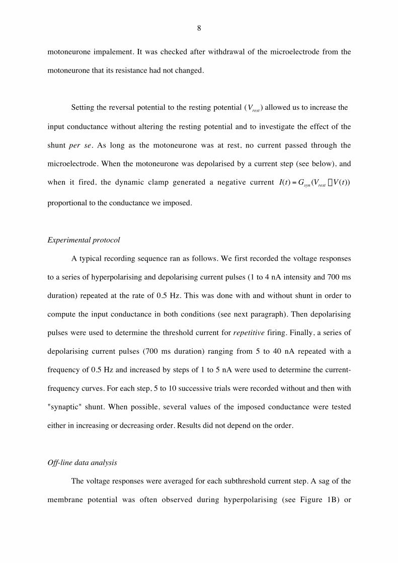
Experimental protocol
A typical recording sequence ran as follows. We first recorded the voltage responses
to a series of hyperpolarising and depolarising current pulses (1 to 4 nA intensity and 700 ms
duration) repeated at the rate of 0.5 Hz. This was done with and without shunt in order to
compute the input conductance in both conditions (see next paragraph). Then depolarising
pulses were used to determine the threshold current for repetitive firing. Finally, a series of
depolarising current pulses (700 ms duration) ranging from 5 to 40 nA repeated with a
frequency of 0.5 Hz and increased by steps of 1 to 5 nA were used to determine the current-
frequency curves. For each step, 5 to 10 successive trials were recorded without and then with
"synaptic" shunt. When possible, several values of the imposed conductance were tested
either in increasing or decreasing order. Results did not depend on the order.
Off-line data analysis
The voltage responses were averaged for each subthreshold current step. A sag of the
membrane potential was often observed during hyperpolarising (see Figure 1B) or
9
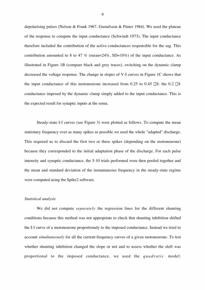
depolarising pulses (Nelson & Frank 1967, Gustafsson & Pinter 1984). We used the plateau
of the response to compute the input conductance (Schwindt 1973). The input conductance
therefore included the contribution of the active conductances responsible for the sag. This
contribution amounted to 8 to 47 % (mean=24%, SD=10%) of the input conductance. As
illustrated in Figure 1B (compare black and grey traces), switching on the dynamic clamp
decreased the voltage response. The change in slopes of V-I curves in Figure 1C shows that
the input conductance of this motoneurone increased from 0.25 to 0.45 mS: the 0.2 mS
conductance imposed by the dynamic clamp simply added to the input conductance. This is
the expected result for synaptic inputs at the soma.
Steady-state I-f curves (see Figure 3) were plotted as follows. To compute the mean
stationary frequency over as many spikes as possible we used the whole "adapted" discharge.
This required us to discard the first two or three spikes (depending on the motoneurone)
because they corresponded to the initial adaptation phase of the discharge. For each pulse
intensity and synaptic conductance, the 5-10 trials performed were then pooled together and
the mean and standard deviation of the instantaneous frequency in the steady-state regime
were computed using the Spike2 software.
Statistical analysis
We did not compute separately the regression lines for the different shunting
conditions because this method was not appropriate to check that shunting inhibition shifted
the I-f curve of a motoneurone proportionaly to the imposed conductance. Instead we tried to
account simultaneously for all the current-frequency curves of a given motoneurone. To test
whether shunting inhibition changed the slope or not and to assess whether the shift was
proportional to the imposed conductance, we used the q u a d r a t i c model:

10
f!=!c1+c2I+c3Gsyn+c4IGsyn+ c5G2syn
(see Graybill 1961). In this model, f was the steady state
firing frequency, I the intensity of the current pulse, and the free parameters c1 to c5 were
determined by data fitting. In all motoneurones, both c4 and c5 were found to be close to zero
indicating that shunting inhibition did not significantly change the slope of the current-
frequency curve and that the shift was proportional to Gsyn. This suggested that a simpler
multi-linear model where f = c1+c2I+c3Gsyn was sufficient to account for the data. We verified
this point using the Fisher
†
F test and found that indeed the quadratic model did not fit our
data better than the linear model. Finally the
†
c 2 test showed that the multi-linear model
provided a good fit, and we used therefore this model to determine the slope and the shift of
the I-f curves.
Results
We report data from 19 lumbar motoneurones (8 CP, 3 TS, 3 Tib, 1 PBSt and 4
Sciatic). These neurones were selected because their resting membrane potential was between
-80 to -51 mV, and the amplitude of their antidromic action potential was in the 70-95 mV
range indicating good microelectrode penetration. In addition, these conditions remained
stable (with variations not larger than 3 mV) during the whole recording sequence that lasted
at least half an hour. Threshold currents for repetitive firing were in the 5 to 21 nA range.
Input conductances ranged from 0.26 to 1.89 mS. Imposed shunting conductances in the 0.1 -
0.5 mS range increased the input conductances by 6 to 109 %. No systematic difference was
seen between pentobarbitone and a-chloralose experiments, and between bridge and DCC
recording modes. Therefore the results were pooled together. Setting the reversal potential to
the resting potential in the dynamic clamp equation (see Figure 1A) and varying the imposed
shunting conductance enabled us to determine in 16 motoneurones how the shunt effect
11
changed the steady-state current-frequency curve. In the 3 remaining neurones we varied both
the imposed conductance and the reversal potential and investigated how this modified the
firing frequency for a given value of the injected current.
Shunting inhibition shifted the I-f curve proportionally to the imposed conductance
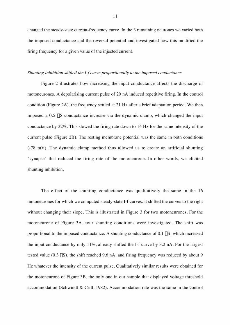
Figure 2 illustrates how increasing the input conductance affects the discharge of
motoneurones. A depolarising current pulse of 20 nA induced repetitive firing. In the control
condition (Figure 2A), the frequency settled at 21 Hz after a brief adaptation period. We then
imposed a 0.5 mS conductance increase via the dynamic clamp, which changed the input
conductance by 32%. This slowed the firing rate down to 14 Hz for the same intensity of the
current pulse (Figure 2B). The resting membrane potential was the same in both conditions
(-78 mV). The dynamic clamp method thus allowed us to create an artificial shunting
"synapse" that reduced the firing rate of the motoneurone. In other words, we elicited
shunting inhibition.
The effect of the shunting conductance was qualitatively the same in the 16
motoneurones for which we computed steady-state I-f curves: it shifted the curves to the right
without changing their slope. This is illustrated in Figure 3 for two motoneurones. For the
motoneurone of Figure 3A, four shunting conditions were investigated. The shift was
proportional to the imposed conductance. A shunting conductance of 0.1 mS, which increased
the input conductance by only 11%, already shifted the I-f curve by 3.2 nA. For the largest
tested value (0.3 mS), the shift reached 9.6 nA, and firing frequency was reduced by about 9
Hz whatever the intensity of the current pulse. Qualitatively similar results were obtained for
the motoneurone of Figure 3B, the only one in our sample that displayed voltage threshold
accommodation (Schwindt & Crill, 1982). Accommodation rate was the same in the control

12
and shunting conditions (0.3 mV/nA). In this motoneurone, 0.25 mS and 0.5 mS shunting
conductances increased the input conductance by 54 and 109%, shifting the I-f curves by 5.8
and 11.6 nA respectively, without any significant change of slope. In all cells, the statistical
analysis (see Methods) confirmed that increasing the input conductance shifted the current-
frequency curve without affecting its slope. In 11 of 16 motoneurones the steady-state I-f
curves were obtained for at least 2 values of the shunting conductance in addition to the
control condition (no shunting conductance). This allowed us to verify that the shift of the
curve was proportional to the shunting conductance. That linear dependence was found even
when the shunting conductance was as large as the input conductance of the neurone (see
Figure 3B). Shunting inhibition thus had the same effect as the injection of a constant
hyperpolarising current, that is, independent of the membrane potential, linearly increasing
with the shunting conductance.
Sensitivity to shunting and shunt potential of motoneurones
The shift of the I-f curve was equal to the shunting conductance times a coefficient
that depended only on the intrinsic properties of the motoneurone. This coefficient had the
dimension of a potential (mV) and could be written as
†
Vshunt -Vrest , where
†
Vshunt was a
potential that we called the shunt potential of the cell. The shunt potential determined the shift
of the current-frequency curve, equal to
†
Gsyn (Vshunt -Vrest ) , for any value of the shunting
conductance, hence its name (see next section and Figure 4 for a more direct definition of the
shunt potential).
The statistical error in the quantity
†
Vshunt -Vrest was smaller than 2 mV in 9 of 16
motoneurones. For these motoneurones, the quantity
†
Vshunt -Vrest ranged from 14 to 37 mV
(mean = 25 mV, SD = 8 mV). This showed that shunting inhibition did not have the same

13
impact on all motoneurones. We could not detect any correlation between the sensitivity to
shunting inhibition, measured by
†
Vshunt -Vrest , and the motoneurone identity, its input
conductance at soma, the slope of its I-f curve, or its axonal conduction velocity. But the lack
of correlation could be due to the small size (N = 9) of our sample.
The shunt potential could be directly measured
Real synapses do not act only through their shunt effect since their reversal synaptic
potential generally differs from the resting membrane potential. When the reversal potential is
below the resting potential, the synapse, in addition to increasing the membrane conductance,
elicits a negative current that hyperpolarises the membrane. This current by itself reduces the
firing frequency and adds to the effect of the shunt. Conversely, when the reversal potential is
above the resting potential a depolarising current results that increases the firing frequency
and competes with shunting inhibition. Using the dynamic clamp, we determined in 3
motoneurones for which values of the reversal potential the shunt effect prevailed over the
depolarisation. Figure 4 shows the results obtained in one of these motoneurones, whose
resting membrane potential was -77 mV. When the reversal potential was set at -70 mV the
shunt effect predominated: despite the depolarisation of the membrane, increasing the
imposed shunting conductance decreased the firing rate. For instance, setting the shunting
conductance to 0.2 mS, that is, increasing the input conductance by 30%, reduced the firing
rate from 27 to 20 Hz. Inhibition decreased with increasing reversal potential, and for a
specific value of the reversal potential (- 60 mV for this neurone) changing the shunting
conductance no longer had any effect on the discharge frequency. For higher values of the
reversal potential the firing rate increased with the shunting conductance indicating that the
depolarising effect prevailed on shunting inhibition. The net effect on the discharge was then

14
excitatory. Similar results were obtained for the other two neurones in which the same
experiment was carried out.
The shunt potential is an intrinsic property of the motoneurone and is not related to
any synaptic reversal potential. However, it coincides in the above protocol with the value of
the reversal potential
†
Erev for which changing the input conductance has no effect on the
firing frequency. Indeed, in this condition the depolarising current
†
Gsyn (Erev -Vrest )
counterbalanced the shift
†
-Gsyn (Vshunt -Vrest ) of the I-f curve elicited by shunting inhibition.
The shunt potential was thus directly determined in the three motoneurones investigated. It
was found to be equal to -60 mV (see figure 4), -40 mV and - 45 mV.
The shunt potential can be interpreted as follows. It takes intermediate values between
the typical reversal potentials of excitatory and inhibitory synapses and indicates whether
mixed excitatory and inhibitory inputs will have a net excitatory or inhibitory effect on the
firing frequency. The firing frequency will increase if the reversal potential of the net synaptic
current is above the shunt potential. On the opposite, the firing frequency will decrease if this
reversal potential is below the shunt potential.
Which cell property determines the shunt potential?
Pooling together the three motoneurones for which the shunt potential was directly
measured (as in figure 4) and the nine motoneurones for which it could be computed from the
shift of I-f curves, we obtained the values of the shunt potential shown in figure 5. The shunt
potential is highly variable, lying between -66 and -33 mV (mean = -45 mV, SD = 9 mV).
This is because the impact of a given synaptic current on the discharge depends on the
response of the neuronal membrane, which varies from cell to cell.
15
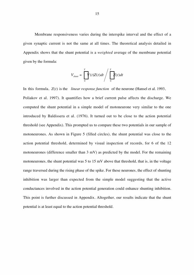
Membrane responsiveness varies during the interspike interval and the effect of a
given synaptic current is not the same at all times. The theoretical analysis detailed in
Appendix shows that the shunt potential is a weighted average of the membrane potential
given by the formula:
†
Vshunt = V (t)0
T
Ú Z(t)dt Z(t)dt0
T
ÚIn this formula,
†
Z(t) is the linear response function of the neurone (Hansel et al. 1993,
Poliakov et al. 1997). It quantifies how a brief current pulse affects the discharge. We
computed the shunt potential in a simple model of motoneurone very similar to the one
introduced by Baldissera et al. (1976). It turned out to be close to the action potential
threshold (see Appendix). This prompted us to compare these two potentials in our sample of
motoneurones. As shown in Figure 5 (filled circles), the shunt potential was close to the
action potential threshold, determined by visual inspection of records, for 6 of the 12
motoneurones (difference smaller than 3 mV) as predicted by the model. For the remaining
motoneurones, the shunt potential was 5 to 15 mV above that threshold, that is, in the voltage
range traversed during the rising phase of the spike. For these neurones, the effect of shunting
inhibition was larger than expected from the simple model suggesting that the active
conductances involved in the action potential generation could enhance shunting inhibition.
This point is further discussed in Appendix. Altogether, our results indicate that the shunt
potential is at least equal to the action potential threshold.

16
Discussion
The goal of the present study was to assess the quantitative effect of shunting
inhibition on the current-frequency curves of cat motoneurones in the primary firing range.
We showed that shunting inhibition could strongly reduce the firing frequency of lumbar
motoneurones and had the same effect on the I-f curve as a constant hyperpolarising current.
This “equivalent” current was proportional to the imposed shunting conductance and
depended on an intrinsic property of the cell that we called its shunt potential. The shunt
potential could be accurately determined in 12 neurones and was 11 to 37 mV above the
resting potential. This spread indicated important differences in the sensitivity of
motoneurones to shunting. The shunt potential was close to the spike voltage threshold in 6
motoneurones and 5 to 15 mV above this threshold for the other 6 neurones (including the
motoneurone of Figure 3B that displayed accommodation). These results were accounted for
by the theoretical analysis presented in Appendix. The shunt potential indicates whether
mixed synaptic inputs will have a net excitatory or inhibitory effect on the ongoing discharge
of the motoneurone.
Comparison with previous studies
Previous experimental studies, carried out on cats anesthetised with barbiturates,
demonstrated that tonic peripheral or descending synaptic inputs did not change the gain of
motoneurones, i.e., the slope of their steady-state I-f curve, in the primary firing range (see the
review of Powers & Binder 2001). The curve was shifted to the left or the right depending on
the balance between excitatory and inhibitory inputs. Similar conclusions were obtained in
recent in vitro studies of cortical (Chance et al. 2002, Ulrich 2003) and cerebellar neurones

17
(Mitchell & Silver 2003): noisy inputs changed the gain of the cell but a constant stimulation
caused only a shift of the I-f curve.
Changes in the slope of I-f curves of motoneurones were observed in other experimental
conditions. Granit et al. (1966b) argued that shifts of the I-f curves were limited to the
primary firing range and that tonic synaptic activity could change the slope in the secondary
range. We did not examine this issue. Our results were limited to the primary firing range
because investigating the secondary range would have required large currents (greater than 40
nA). Such currents would have induced electrode polarization and could have deteriorated the
spiking mechanism because of long-lasting inactivation of the sodium current. Kernell (1966)
observed an increase of the slope in the primary range during repetitive stimulation of the
brainstem. This was associated with a decreased afterhyperpolarisation likely due to
neuromodulatory inputs. Similar effects were reported by Brownstone et al. (1992) during
fictive locomotion in decerebrate cats. The slope of the current-frequency curve increased
during episodes of locomotion and returned back to the control value when locomotion
stopped. In contrast, Shapovalov & Grantyn (1968) observed that a repetitive stimulation of
the reticular formation elicited either a simple shift of the I-f curve or a reduction of the slope
in chromatolysed motoneurones.
It is widely believed that the shift of the I-f curve, elicited by tonic synaptic activation, is
equal to the average synaptic current, acting at the soma (Powers & Binder 1995, Holt &
Koch 1997, Ulrich 2003). But this stems from a reasoning error. When the motoneurone
discharges, intrinsic active conductances, such as the afterhyperpolarisation conductance, vary
during the interspike interval. They shape the voltage trajectory and the response of the
membrane to synaptic inputs. In these conditions, the shift of I-f curves is determined by both

18
the synaptic input and the membrane response function. The shift would be equal to the
average synaptic current only if the response of the membrane was the same at all time, which
is not true (see figure 6 in Appendix).
In our study, we focussed on the sensitivity of motoneurones to shunting inhibition. A
single study previously addressed this issue (Schwindt & Calvin, 1973b). The authors did not
observe significant shifts of I-f curves when synaptic inputs elicited by an electrical
stimulation of a hindlimb nerve increased the input conductance of lumbar motoneurones, by
as much as 70%, with little effect on the resting membrane potential. The fact that I-f curves
were not shifted suggest that the shunt potential was close to the reversal potential of the net
synaptic current and therefore near the resting membrane potential. However, we never
observed such situation in our experiments: the shunt potential was always close to the
voltage threshold for spiking or above it, exceeding the resting potential by at least 11 mV.
Functional implications
Our results suggest that inhibitory synapses, which are mainly located on the soma or
on proximal dendrites (see for instance Burke et al. 1971, Fyffe 1991), largely act through
their shunting inhibition. Indeed the efficacy of shunting inhibition is measured by
†
Vshunt -Vrest
that ranged from 11 to 37 mV in the present study. This is about twice the driving force of
inhibitory synapses, the reversal potential of which is 5 to 20 mV below the resting potential
(Coombs et al. 1955a). The added effects of the hyperpolarisation and of the shunt endow
inhibitory synapses with an efficacy comparable to that of excitatory synapses. Therefore,
shunting inhibition is likely a major operating mode of the inhibitory systems acting on
motoneurones (Ia reciprocal inhibition, Ib inhibition, recurrent inhibition, etc.).

19
Our results were obtained in motoneurones of anesthetised animals. In these animals,
the discharge of motoneurones is controlled by the slow afterhyperpolarisation current.
Responsiveness to synaptic inputs is high only near the end of the interval. This fully explains
all observed features of shunting inhibition: constancy of the slope of I-f curve, shift of the
curve proportional to shunting conductance, and shunt potential close to the spike threshold or
above it (see theoretical analysis in Appendix). Experiments in non-anaesthetised and
decerebrated cats indicate that neuromodulatory inputs may place motoneurones in another
state in which afterhyperpolarisation is reduced and persistent inward currents are expressed
(see, for instance, Hounsgaard et al. 1988, Brownstone et al. 1992, Bennett et al. 1998, and
the review on this point in Powers & Binder 2001). Both experimental and modelling studies
have shown that reducing the conductance responsible for afterhyperpolarisation increases the
firing frequency of motoneurones and the slope of their current-frequency curve (Kernell
1966, Kernell 1968, Zhang & Krnjevic 1987). However, we expect that the reduction of
afterhyperpolarisation conductance will have little impact on the shunt potential, because the
response function will still peak at the end of the interspike interval. In contrast, the activation
of persistent inward currents dramatically alters the excitability of motoneurones and thereby
their response function. It is difficult to speculate on the impact of persistent inward currents
on shunting inhibition, all the more as inhibitory synapses can reduce these currents (Hultborn
et al. 2003, Kuo et al. 2003). The interplay between shunting inhibition and persistent inward
currents largely remains to be explored.

20
Appendix
To understand how a constant shunting conductance affects the discharge of
motoneurons in our experiments one must determine the response properties of the
membrane. The impulse response
†
Z(t) tells us by how much a brief current pulse at time
†
t
shifts the spike train (Hansel et al. 1993). The effect of the shunting current is obtained by
summing the effects of elementary impulses: the interspike intervals increase by
†
DT = Gsyn0
T
Ú Vrest -V (t)( )Z(t)dt . A priori, this linear summation holds true only when the
shunting current is small. From the formula above, one deduces the variation
†
Df = -DT T 2 of
the firing frequency and the shift of the I-f curve
†
DI = Gsyn Vrest -V (t)( )0
T
Ú Z(t)dt Z(t)dt0
T
Ú .
Comparison with the formula
†
DI = Gsyn Vrest -Vshunt( ) previously established allows us to
conclude that
†
Vshunt = V (t)0
T
Ú Z(t)dt Z(t)dt0
T
Ú (A1)
This shows that the shunt potential is a weighted average of the membrane potential. The
weighting factor is the normalised response function
†
Z(t) / Z(t)dt0
T
Ú .
We computed the response function of a single compartment integrate-and-fire model
of the motoneurone (Kernell 1968, Baldissera et. al. 1976, Meunier & Borejsza, unpublished
observations). The voltage evolution equation for this model reads
†
CmdV (t)
dt= -Gm V (t) -Vrest( ) + GAHP (t) VK -V (t)( ) + I (A2)

21
where
†
Cm is the membrane capacitance,
†
Gm the passive conductance,
†
GAHP the conductance
of the slow current responsible for afterhyperpolarisation that exponentially decays,
†
VK the
Nernst potential of potassium ions, and
†
I the current pulse that elicits repetitive firing with
period
†
T . Every time the potential reaches the fixed spike threshold
†
Vth an action potential is
emitted, and voltage is reset to the value
†
Vreset .
When a brief inhibitory current pulse
†
dI(t) = qd t - t *( ) delivers at time
†
t * a small
negative charge
†
q to the neurone, it produces a voltage drop
†
dV (t*) = q /Cm . This voltage
perturbation relaxes according to
†
CmddVdt
= -G(t)dV where
†
G(t) = Gm + GAHP (t) is the
membrane conductance at time
†
t . At time T, a residual perturbation of the potential
†
dV (T) = dV (t*)exp - dt 'G(t ') /Ct*
T
ÚÊ
Ë Á
ˆ
¯ ˜ is still present. As a consequence, the interspike interval
is lengthened by the amount
†
dT1 that is computed by dividing
†
dV (T) by the time derivative of
the voltage. The following intervals are also modified because lengthening an interval slightly
decreases the AHP conductance in the next interval. After a while the discharge is again
regular, but spikes are shifted by a quantity proportional to
†
dT1 . This proves that
†
Z(t) is
proportional to
†
exp - dt 'G(t ') /CtTÚ( ) .
The normalised response function is displayed in Figure 6A. It is close to
†
0 on most of
the interspike interval and it sharply rises near the end of the interval. This can be explained
as follows. When a voltage perturbation occurs early in the interspike interval, it relaxes
before the end of the interval and has a negligible effect on the timing of the next spike. In
contrast, when the perturbation occurs at the end of the interval, the following spike is
delayed until the perturbation has relaxed. Because our model is linear below the voltage

22
threshold, the response function accounts for the effects of shunting currents even when the
shunting conductance is comparable to the input conductance. The shift of the I-f curves is
proportional to the shunting conductance and the shunt potential, computed from equation
(A1), is close to the voltage threshold. The model thus accounts for the linearity of the shift
observed in all motoneurones of our sample and for the values of the shunt potential close to
voltage threshold obtained in half of the motoneurones.
Because our model is restricted to the subthreshold voltage range and does not
incorporate the currents responsible for action potentials, it cannot explain why the shunt
potential was larger than the voltage threshold in the other half of our sample. Poliakov et al.
(1997) determined experimentally the response function of cat lumbar motoneurones (see an
example in Figure 6B). It decays fast but not instantaneously to zero at the end of the
interspike interval, in contrast to the model. Using the experimental response function (Figure
6B), we computed the shunt potential from equation (A1) and found
†
Vshunt ª -52mV , which was
very close to the spike threshold potential measured on the voltage trace. This is because the
decay phase of the response function does not overlap the rising phase of the action potential.
A substantial overlap would increase much the product
†
V t( )Z t( ) , and would lead to shunt
potentials well above the action potential threshold. We tested this idea by shifting to the right
by 0.3 or 0.5 ms the response function of Figure 6B. The shunt potential increased indeed by
3.5 and 11 mV respectively. This suggests that small changes in the response properties of
motoneurones may considerably increase
†
Vshunt and explain the spread of the shunt potential
observed in our sample, up to values15 mV above the action potential threshold.
23
References
Baldissera F, Gustafsson B & Parmiggiani F (1976). A model for refractoriness accumulationand secondary range firing in spinal motoneurones. Biol Cyber 24, 61-65.
Bennett DJ, Hultborn H, Fedirchuk B & Gorassini M (1998). Synaptic activation of plateausin hindlimb motoneurones of decerebrate cats. J. Neurophysiol 80, 2023-2037.
Brizzi L, Hansel D, Meunier D, Van Vreeswijk C & Zytnicki D (2001). Shunting inhibition: a
study using in vivo dynamic clamp on cat spinal motoneurons. Soc Neurosci Abstr 27, 934.3
Brownstone RM, Jordan LM, Kriellaars DJ, Noga BR & Schefchyk SJ (1992). On the
regulation of repetitive firing in lumbar motoneurones during fictive locomotion in the cat.Exp Brain Res 90, 441-455.
Burke RE, Fedina L & Lundberg A (1971). Spatial synaptic distribution of recurrent and
group Ia inhibitory systems in cat spinal motoneurones. J Physiol (Lond) 214, 305-326.
Capaday C (2002). A re-examination of the possibility of controlling the firing gain of
neurons by balancing excitatory and inhibitory conductances. Exp Brain Res 143, 67-77.
Chance FS, Abbott LF & Reyes AD (2002). Gain modulation from background synapticinput. Neuron 35, 773-782.
Coombs JS, Eccles JC & Fatt P (1955a). The specific ionic conductances and the ionicmovements across the motoneuronal membrane that produce the inhibitory post-synaptic
potential. J Physiol (Lond) 130, 326-373.
Coombs JS, Eccles JC & Fatt P (1955b). The inhibitory suppression of reflex discharges frommotoneurones. J Physiol (Lond) 130, 396-413.
Cymbalyuk GS, Gaudry Q, Masino MA & Calabrese RL (2002) Bursting in leech heartinterneurons: cell-autonomous and network-based mechanisms. J Neurosci 22, 10580-10592.
Fyffe RE (1991) Spatial distribution of recurrent inhibitory synapses on spinal motoneurons
in the cat. J Neurophysiol 65,1134-1149.
Gosnach S, Quevedo J, Fedirbuck B & McCrea DA (2000). Depression of group Ia
monosynaptic EPSPs in cat hindlimb motoneurones during fictive locomotion. J Physiol
(Lond) 526, 639-652.

24
Granit R, Kernell D & Lamarre Y (1966a). Algebrical summation in synaptic activation of
motoneurones firing within the primary range to injected currents. J Physiol (Lond) 187, 379-
399.
Granit R, Kernell D & Lamarre Y (1966b). Synaptic stimulation superimposed on
motoneurones firing in the 'secondary range' to injected current. J Physiol (Lond) 187, 401-415.
Graybill FA (1961). An introduction to linear statistical models. McGraw-Hill, New-York.
Gustafsson B & Pinter J (1984). Relations among passive electrical properties of lumbar a-
motoneurones of the cat. J Physiol (Lond) 356, 401-434.
Hansel D, Mato G & Meunier C (1993). Phase reduction and neural modeling, Concepts
Neurosci 4,193-210.
Holt GR & Koch C (1997). Shunting inhibition does not have a divisive effect on firing rates.Neural Comput 9, 1001-1013.
Hounsgaard J, Hultborn H, Jespersen B & Kiehn O (1988). Bistability of alpha-motoneuronesin the decerebrate cat and in the acute spinal cat after intravenous 5-hydroxytryptophan. J
Physiol (Lond) 414, 345-367.
Hultborn H, Enriquez-Denton M., Wienecke J & Nielsen JB (2003). Variable amplification ofsynaptic input to cat spinal motoneurones by dendritic persistent inward current. J Physiol
(Lond) 552, 945-952.
Kernell D (1966). The repetitive discharge of motoneurones. In Muscular afferents and motor
control, ed. Granit R, pp. 351-362. John Wiley & Sons, New-York, London, Sydney &
Almqvist & Wiksell, Stockholm.
Kernell D (1968). The repetitive impulse discharge of a simple neurone model compared to
that of spinal motoneurones. Brain Res 11, 685-687.
Kuo JJ, Lee RH, Johnson MD, Heckman HM & Heckman CJ (2003) Active dendritic
integration of inhibitory synaptic inputs in vivo. J Neurophysiol 90, 3617-3624
Le Masson G, Renaud-Le Masson S, Debay D & Bal T (2002) Feedback inhibition controlsspike transfer in hybrid thalamic circuits. Nature 417, 854-858.
Manor Y, Yarom Y, Chorev E & Devor A (2000) To beat or not to beat: a decision taken at
the network level. J Physiol (Paris) 94, 375-390.

25
Mitchell SJ & Silver AR (2003). Shunting inhibition modulates neuronal gain during synaptic
excitation. Neuron 38, 433-445.
Nelson PG & Frank K (1967). Anomalous rectification in cat spinal motoneurons and effectof polarizing currents on excitatory post-synaptic potentials. J Neurophysiol 30, 1097-1113.
Perreault M-C (2002). Motoneurons have different membrane resistance during fictivescratching and weight support. J Neurosci 22, 8259-8265.
Poliakov AV, Powers RK & Binder MD (1997). Functional identification of the input-output
transforms of motoneurones in the rat and cat. J Physiol (Lond) 504, 401-424.
Powers RK & Binder MD (1995). Effective synaptic current and motoneuron firing rate
modulation. J Neurophysiol 74, 793-801.
Powers RK & Binder MD (2001). Input-output functions of mammalian motoneurons. Rev
Physiol Biochem Pharmacol 143, 137-263.
Prinz AA, Abbott LF & Marder E (2004) The dynamic clamp comes of age. TINS 27, 218-224.
Robinson HP & Kawai N (1993). Injection of digitally synthesized synaptic conductance
transients to measure the integrative properties of neurons. J Neurosci Meth 49, 157-165.
Schwindt PC (1973). Membrane-potential trajectories underlying motoneuron rhythmic firing
at high rates. J Neurophysiol 36, 434-449.
Schwindt PC & Calvin WH (1973a). Equivalence of synaptic and injected current in
determining the membrane potentiel trajectory during motoneuron rhythmic firing. Brain Res
59, 389-394.
Schwindt PC & Calvin WH (1973b). Nature of conductances underlying rhythmic firing cat
spinal motoneurons. J Neurophysiol 36, 955-973.
Schwindt PC & Crill WE (1982). Factors influencing motoneuron rythmic firing: results
from a voltage-clamp study. J Neurophysiol 48, 875-890.
Shapovalov AI & Grantyn AA (1968). Suprasegmental synaptic effect on chromatolyzedmotor neurons. Biofizika 13, 260-269.
Sharp AA, O'Neil MB, Abbott LF & Marder E (1993). Dynamic clamp: computer-generatedconductances in real neurons. J Neurophysiol 69, 992-995.

26
Shefchyk SJ & Jordan LM (1985). Motoneuron input-resistance changes during fictive
locomotion produced by stimulation of the mesencephalic locomotor region. J Neurophysiol
54, 1101-1108.
Shriki O, Hansel D & Sompolinsky H (2003). Rate models for conductance-based cortical
neuronal networks. Neural Comput. 15, 1809-41.
Ulrich D (2003). Differential arithmetic of shunting inhibition for voltage and spike rate in
neocortical pyramidal cells. Eur J Neurosci 18, 2159-2165.
Zhang L & Krnjevic K (1987). Apamin depresses selectively the after-hyperpolarization ofcat spinal motoneurons. Neurosci. Lett. 74, 58-62.
Acknowledgements
Financial supports provided by Délégation Générale pour l'Armement (DGA Grant 0034029)and by Ministère de la Recherche (Action Concertée Incitative "Neurosciences Intégratives et
Computationnelles") are gratefully acknowledged. We are indebted to Dr. C. Capaday for
stimulating discussions about this work. The authors wish to thank Drs. M. Buiatti, L.Graham and L. Jami for helpful comments and M. Manuel and A. Roxin for careful
scrutinising of the manuscript.

27
Figure legends
Figure 1: Increase of the motoneurone input conductance imposed by the dynamicclampA. Schematic diagram of the experimental set up for dynamic clamp. Repetitive firing of the
motoneurone was elicited by an intracellular current pulse generated with the step command
of the Axoclamp 2B. The membrane potential was digitized with an Analog to DigitalConverter (ADC) and low-pass filtered (see text). For each value of the membrane potential,
the Power 1401 unit computed the current to be injected in the motoneurone through theintracellular microelectrode. This current was then converted in a voltage by a Digital to
Analog Converter (DAC). The resulting clamp signal was fed into the current injection circuit
of the Axoclamp 2B where it was added to the current pulse.B. Voltage response of a common peroneal motoneurone to a 4 nA hyperpolarising current
pulse of 700 ms duration. Responses (average of 4 successive records) without (grey trace)and with the dynamic clamp feedback (black trace,
†
Gsyn = 0.2 µS). The plateau response was
defined as the difference between the resting potential and the mean voltage during the last
0.5 s (horizontal bar below the trace). In dynamic clamp condition plateau response was
reduced by 44%. Note that the voltage sag was particularly small in this motoneurone (sagconductances contributed only 8% to the input conductance) and almost disappeared in the
dynamic clamp condition.
C. Same motoneurone as in B. V-I curves obtained without (grey triangles) and with (blackcircles) dynamic clamp feedback imposing a 0.2 µS increase of the input conductance.
Regression lines superimposed. Voltages were computed during the plateau (see B).Therefore, the slope of the regression line did not provide the passive input conductance but
also included the contribution of the sag conductance. As expected, the slope of the V-I curve
decreased from 3.9 to 2.2 MW (0.25 and 0.45 µS input conductance, respectively). Note that,
for the small currents injected, V-I curves did not significantly depart from linearity. This wasalso the case for the other recorded motoneurones, though they exhibited larger voltage sags.
Figure 2: How a conductance increase affects the firing rateComparison between the control condition (A) and a dynamic clamp condition where Gsyn =0.5 µS (B). Upper traces: membrane potential, middle traces: current pulse, lower traces: extra
28
conductance imposed by the dynamic clamp. Increasing the input conductance via the
dynamic clamp did not affect the resting membrane potential, which remained at -78 mV (B,
upper trace). Therefore the reduction of the firing rate followed only from the inputconductance increase, i.e., from shunting inhibition. Note that the hyperpolarisation after the
end of the pulse was smaller in B than in A because i) the last spike occurred 20 ms earlier inB than in A, so that by the end of the pulse, afterhyperpolarisation had partially relaxed, and
ii) the larger membrane conductance in B reduced the amplitude of afterhyperpolarisation.
Records from a sciatic motoneurone with an input conductance of 1.56 µS in the absence ofdynamic clamp (condition A).
Figure 3: Effect of shunting inhibition on I-f curvesI-f curves in control (empty squares) and several shunting conditions (filled symbols). Eachdot represents the mean instantaneous frequency in the steady-state regime for a given value
of the injected current, the associated vertical bar indicating the standard deviation. Multi-
linear regression lines (see Methods) are also displayed.A. CP motoneurone with an input conductance of 0.89 mS. Three shunting conditions were
investigated : Gsyn = 0.1 µS (circles), 0.2 µS (triangles), and 0.3 µS (diamonds).
B. TS motoneurone with an input conductance of 0.46 µS. This motoneuron was the only onein our sample that displayed voltage threshold accommodation. Two shunting conditions were
investigated : Gsyn = 0.25 µS (circles), and Gsyn= 0.5 µS (triangles).
In both motoneurones, the conductance increase shifted the curves without altering theirslope, and the shift was proportional to Gsyn. Note that in dynamic clamp conditions we did
not try to adjust the injected current to reach the minimum firing frequency.
Figure 4: Effect of the reversal potential on the discharge frequencyThe 3D diagram shows how the discharge frequency was modified by the conductance
increase for three values of the reversal potential (-70, -60 and -50 mV). A depolarising
current pulse (16 nA, 700 ms) was used to elicit firing. The ordinate is the variation of thedischarge frequency with respect to the control condition (i.e., when
†
Gsyn = 0). For
†
Erev = -60
mV, increasing
†
Gsyn had almost no effect on the firing rate of the motoneurone. This value
corresponds to the shunt potential. When the reversal potential was greater than the shunt
29
potential, the net effect was excitatory (increase of the firing rate with the imposed
conductance). In the opposite case the net effect was inhibitory (decrease of the firing rate).
†
Vrest = - 77 mV. Tib motoneurone with an input conductance of 0.67 µS.
Figure 5: Relationship between the shunt potential and the action potential thresholdThe shunt potential was directly measured for 3 motoneurones (open circles) and computed asexplained in the text for the 9 other motoneurones (filled circles). The action potential
threshold, defined as the voltage where the spike upstroke began, was determined by visual
inspection in control condition (no shunt) for the lowest injected current. This simpleprocedure proved to be more accurate than relying on the voltage derivative because of the
noisiness of the traces. Vertical and horizontal bars indicate standard errors on the shuntpotential and the action potential threshold respectively. The error in the shunt potential takesinto account both the statistical error in
†
Vshunt -Vrest and the uncertainty in the measurement of
the resting potential. Errors in the action potential threshold arise from recording noise andvariations of the threshold during the train. The oblique line is the bisectrix along which the
shunt potential equals the action potential threshold. Measurements made in the
accommodating motoneurone of Figure 3B are indicated by arrows.
Figure 6: Response properties of an integrate-and-fire model (A) and of a cat lumbarmotoneurone (B).A. Model described in Appendix. The resting potential is set to 0, the voltage threshold to 1,
the reset potential following the spike to 0.6 and the Nernst potential of potassium to -1.Conductance of the slow afterhyperpolarisation current following the first spike equals the
input conductance. Passive membrane time constant: 5 ms, relaxation time constant ofafterhyperpolarisation : 25 ms, firing frequency : 10 Hz. Thick trace: normalised response
function , thin trace : membrane potential normalised with respect to the action potential
threshold.B. Spike-evoking current (thick trace) and membrane potential (thin trace) as measured by
Poliakov et al. (1997). A 10 nA current injected in the motoneurone elicited a repetitivedischarge. Gaussian white noise was added to it and perturbed spike timing. The two traces

30
were obtained by spike-triggered averaging. The linear response function is proportional to
the spike evoking current minus the 10 nA baseline (see Poliakov et al. 1997).