THE CENTRE FOR MARKET AND PUBLIC ORGANISATION

Centre for Market and Public Organisation Bristol Institute of Public Affairs

University of Bristol 2 Priory Road

Bristol BS8 1TX http://www.bristol.ac.uk/cmpo/

Tel: (0117) 33 10952 Fax: (0117) 33 10705

E-mail: cmpo-admin@bristol.ac.uk The Centre for Market and Public Organisation (CMPO) is a leading research centre, combining expertise in economics, geography and law. Our objective is to study the intersection between the public and private sectors of the economy, and in particular to understand the right way to organise and deliver public services. The Centre aims to develop research, contribute to the public debate and inform policy-making. CMPO, now an ESRC Research Centre was established in 1998 with two large grants from The Leverhulme Trust. In 2004 we were awarded ESRC Research Centre status, and CMPO now combines core funding from both the ESRC and the Trust.

ISSN 1473-625X

How should we treat under-performing schools? A regression

discontinuity analysis of school inspections in England

Rebecca Allen and Simon Burgess

March 2012

Working Paper No. 12/287

CMPO Working Paper Series No. 12/287

How should we treat under-performing schools? A regression discontinuity

analysis of school inspections in England

Rebecca Allen1 and Simon Burgess2

1Institute of Education, University of London

2 CMPO, University of Bristol

March 2012

Abstract School inspections are an important part of the accountability framework for education in England. In this paper we use a panel of schools to evaluate the effect of a school failing its inspection. We collect a decade’s worth of data on how schools are judged across a very large range of sub-criteria, alongside an overall judgement of effectiveness. We use this data within a fuzzy regression discontinuity design to model the impact of ‘just’ failing the inspection, relative to the impact of ‘just’ passing. This analysis is implemented using a time-series of school performance and pupil background data. Our results suggest that schools only just failing do see an improvement in scores over the following two to three years. The effect size is moderate to large at around 10% of a pupil-level standard deviation in test scores. We also show that this improvement occurs in core compulsory subjects, suggesting that this is not all the result of course entry gaming on the part of schools. There is little positive impact on lower ability pupils, with equally large effects for those in the middle and top end of the ability distribution. Keywords: School inspection; school accountability; school attainment; regression discontinuity JEL Classification: I20, I28 Electronic version: www.bristol.ac.uk/cmpo/publications/papers/2012/wp287.pdf Acknowledgements We are very grateful to Ofsted for retrieving policy documents and data from their archives and to the Department for Education for providing access to the National Pupil Database. Interpretation of our findings has been aided through a large number of conversations with policy officials at Ofsted, former school inspectors and headteachers. We are grateful for useful comments to seminar audiences at NIESR, the Institute of Education and University of Cambridge. Particular thanks to Mike Brewer, Jane Cooley Fruehwirth, Hamish Low and Iftikhar Hussain for reading drafts and discussing ideas. Address for correspondence CMPO, Bristol Institute of Public Affairs University of Bristol 2 Priory Road Bristol BS8 1TX Simon.burgess@bristol.ac.uk www.bristol.ac.uk/cmpo/

2

1. Introduction

What is the best policy for dealing with under-performing schools? Most education systems have a

mechanism for identifying such schools, typically an inspection system where an external body is

responsible for monitoring and reporting on educational standards. But what should then be done

with schools which are highlighted as failing their pupils? There are important trade-offs to be

considered: rapid intervention may be an over-reaction to a freak year of poor performance, but a

more measured approach may leave many cohorts of students to under-achieve. Similarly, it is hard

to impose penalties alongside greater support, but it is unclear which is more likely to turn a school

around. Designing a process of intervention is important even in a market-based system where we

might hope that new pupils shun failing schools because we must protect the interests of children

whose parents do not exercise choice or who remain ‘loyal’ to a local school.

In this paper, we evaluate the effect of making and publicly announcing an inspection judgement of

‘unsatisfactory’ on poorly performing secondary schools in England. Such schools are identified by a

national school inspection body, Ofsted (the Office for Standards in Education, Children’s Services

and Skills).1 On the basis of its on-site inspections, Ofsted’s judgement of ‘unsatisfactory’ triggers a

set of policy actions, described below. We evaluate the impact of this intervention on overall school

performance in high-stakes national tests at age 16 over different time horizons, on test scores in

maths and English specifically, and test for differential impact on students of different ability. We

also analyse the effect on demand for places in the school. We implement a regression discontinuity

design (RDD) in a panel data context, comparing the time series of performance statistics for schools

that are designated as just failing with those just passing. By dealing with the obvious endogeneity of

failure, this approach estimates the causal impact of that policy on school performance. The

intuition behind an RDD in this context is that schools around the failure threshold are very similar,

except for as-good-as-random measurement of quality by inspectors that causes some schools to

just pass their inspection while others just fail. The converse of the strong internal validity of the

RDD approach is weaker external validity. Schools which fail their inspection by a considerable

margin may react very differently to their failure, and we make no claims about the applicability of

our results to severely failing schools. We return to this issue in the Conclusion.

In principle, the effects of failing an Ofsted inspection could go either way: it could be a catalyst for

improvement or a route to decline. It could lead to improved performance if it induces the school to

work harder to pass a subsequent inspection: more focussed leadership and more effective teaching

1 See http://www.ofsted.gov.uk/about-us , accessed 10/10/11.

3

could raise test scores. On the other hand, if students and teachers leave the school, the failure may

trigger a spiral of decline where falling rolls lead to low morale, financial difficulties and even lower

test scores. So it is a meaningful question to ask whether test scores improve or worsen following

the treatment.

This paper contributes to a large international literature on the effect of school inspections and

sanctions. In the US a large literature has focussed on the accountability mechanisms built into the

No Child Left Behind Act.2 Our RDD approach and our findings bear similarities to Fruehwirth and

Traczynski (2011) and to Ahn and Vigdor (2009), who both find that schools in North Carolina facing

sanctions under No Child Left Behind (NCLB) improve performance. The former confirms Neal and

Schanzenbach’s (2010) finding that schools facing these forms of accountability tend to focus on

students at the threshold of performance measures at the expense of the lowest performing pupils.

In the UK, there are fewer studies of the dual accountability systems of publicly published

performance tables3 and Ofsted inspections. Rosenthal (2004) studies the impact of Ofsted visits and

has a negative conclusion: there is no gain after the visit and there is a fall in performance in the year

of the visit. Using a more sophisticated econometric approach, Hussain (2012) identifies the very

short-term impact of failing an inspection in primary schools. He compares the performance of

schools failed early in the academic year with those failed later in the academic year, specifically

after pupil exams. This identification strategy compares like with like, and isolates the effect of

having some 8 months to respond to the failure. Our approach differs by focussing on the high-

stakes exams at the end of compulsory school, by using a panel data run of 10 years to estimate

longer-term effects, and by adopting a different identification strategy that allows us to leverage in

more data.

We find that schools failing their Ofsted inspections improve their subsequent performance relative

the pre-visit year. The magnitudes are quantitatively very significant: around 10% of a (student-level)

standard deviation or one grade in between one and two of their best eight exam subjects. The main

impact arises two years after the visit in this data – not unreasonable given that the exam scores we

use derive from two-year courses. The typical time pattern in our results is little effect in the first

post-visit year, increasing considerably the following year, then remaining flat or slightly increasing

in the third post-visit year.

2 This includes Reback (2008), Jacob (2005), Neal and Schanzenbach (2010), Rockoff and Turner (2010), Figlio and Rouse

(2006), and Chakrabarti (2010), Dee and Jacob (2011), Krieg (2008); Ladd and Lauen (2010], and Ahn and Vigdor (2009). 3 For example, Burgess et al (2010) show that the publication of league tables does have an impact on school performance,

and Allen and Burgess (2011) show that league tables are useful to parents in choosing schools.

4

In the next section we set out the policies in England regarding school inspections and describe the

nature of the treatment received by schools judged to be failing their pupils. In section 3 we describe

our data and our identification strategy. The results are in section 4. In the final section we conclude

with some comments on the role of these policies in a suite of responses to poorly performing

schools.

2. Policy Background

Most countries in the world operate a inspection system where an external body is responsible for

monitoring and reporting on educational standards within schools. The nature and purpose of the

inspection systems varies considerably. Coleman (1998) describes a continuum with one extreme as

the objectives-based approach which has the features of being summative, external and formal,

focusing on simply judging whether externally pre-determined objectives for education are being

achieved. These types of high-stakes inspections play an important part in an accountability

framework by giving parents and officials information about school quality that they can act on,

should they wish to. At the other end of a continuum of inspections is a process-based approach

which is much more formative, internal and informal and looks to take value from the process of

inspection as it advises, supports and helps to improve the education provider. The English schools

inspectorate is firmly at the summative, high stakes end of this spectrum.

2.1 The English school inspection system

The Office for Standards in Education, Children’s Services and Skills, known as Ofsted, was created in

the 1992 Education Act as part of a new era of parental choice and accountability. It is a national

body that provides regular independent inspection of schools with public reporting to both parents

and Parliament, and the provision of advice to ministers. The current intended role of Ofsted is “to

provide an independent external evaluation of a school’s effectiveness and a diagnosis of what the

school should do to improve, based on a range of evidence including that of first-hand observation”

(Ofsted, 2011a, page 4). The Inspectorate has focused on the need to make schools accountable for

their performance and thus has placed great emphasis on the use of external examination results

along with ‘snapshot’ external inspections to judge schools (Learmonth, 2000). The criteria on which

schools are evaluated are both objective, such as exam results, and subjective, such as the

inspectors’ view of teaching quality observed during inspections. While the model is formal and

accountability focused, giving both judgments on individual schools and the system as a whole, it

does have elements of support and improvement through mechanisms such as school action plans.

5

The legal requirement is for schools to be inspected on a five year cycle. Since 2005, the frequency

of inspections is proportionate to perceived need such that schools judged satisfactory will be on a

three year cycle and schools judged as unsatisfactory will be visited more frequently and without

notice. The period of notice schools receive before an inspection has shrunk over time from over

two months’ notice to the current period of between zero and two working days, with no notice

possible where there are concerns relating to pupils’ welfare, safeguarding, where the school’s

academic performance has shown rapid decline or where concern is raised by parents.

School inspections are currently conducted by Her Majesty’s Inspectors (HMI), who are employed by

Ofsted, and additional inspectors, who are employed full-time, freelance or otherwise commercially

contracted by Ofsted’s inspection service providers (CfBT, Tribal and Serco). The intensity of the

visits has fallen considerably over time, with full scale week-long visits by a large team of inspectors

prior to the 2005 inspection reforms. Since September 2005 visits are shorter in duration (around

two days) and reliant on fewer inspectors in the school. They are more sharply focused on the

school’s own self-evaluation of their strengths and weaknesses and particularly focus on

management, including how well the school is managed, what processes are in place to ensure

standards of teaching and learning improve, and how well the management team understand their

own strengths and weaknesses.

2.2 The inspection process and the policy treatment

Before a visit, inspectors draw on attainment data, school performance indicators and reports from

previous inspections to decide how to plan their inspection. During the visit, inspectors usually talk

with pupils, governors, management and staff to gather specific views on provision, observe a large

number of lessons, ‘track’ individual pupils to monitor provision for specific groups and scrutinise

school records and documentation (Ofsted, 2011a). Parents and staff are always invited to give their

views on the school in a short questionnaire. Inspectors considering a judgement of ‘unsatisfactory’

will typically discuss the case with another inspector on the phone to utilise a broader range of

experience and will have the findings of their inspection subjected to moderation by the Chief

Inspector.

Inspectors base their overall view of a school on a series of sub-judgements about different aspects

of the school. For example, during 2009 judgements were made about pupil outcomes (7 sub-

criteria), quality of provision (3 sub-criteria), leadership and management (8 sub-criteria), and early

years, sixth form and boarding provision where relevant (Ofsted, 2011a). Under the post-2005

framework a school immediately receives one of four overall judgements: outstanding, good,

satisfactory or unsatisfactory/inadequate. The impact of this last judgment is the subject of this

6

paper. The overall judgement first became very prominent in the inspection report in the academic

year 2002/3, which by law must be delivered to parents of children at the school.

Those schools judged to be unsatisfactory are deemed to have ‘failed’ their Ofsted inspection. These

schools are currently split into two categories of schools causing concern: schools given ‘Notice to

Improve’ and schools placed in ‘Special Measures’. Notice to Improve means that “the school

requires significant improvement because either: it is failing to provide an acceptable standard of

education, but is demonstrating the capacity to improve; or it is not failing to provide an acceptable

standard of education but is performing significantly less well in all the circumstances reasonably be

expected to perform” (Ofsted, 2011a, page 12). Special Measures is a more serious judgement

against a school, meaning that “the school is failing to give its pupils an acceptable standard of

education and the persons responsible for leading, managing or governing the school are not

demonstrating the capacity to secure the necessary improvement in the school” (Ofsted, 2011a, page

12).4

While our sample includes all inspection failures, our use of the RD design means that we use for

estimation only the marginal fails. These are therefore the schools given Notice to Improve, rather

than schools put in Special Measures, and so it is this policy treatment that is the focus of our paper.

There are two components: the public announcement of the judgement, and the internal pressure

on schools. The ‘naming and shaming’ of failing schools is a significant part of the process, and is

typically widely reported in the local media. This stigma of failure is likely to be the most significant

factor for many Headteachers and school governors. Otherwise, the treatment is neither strongly

punitive nor strongly supportive. These schools are subject to no operating restrictions and will

simply receive a monitoring inspection between six and eight months after the publication of their

inspection report.5 They will also be fully inspected around a year after their Notice to Improve was

served (this will be generally carried out by a different inspector). The headteacher, chair of the

governing body and a representative from the local authority or proprietor will have been invited to

attend a school improvement seminar, but there is no requirement for them to attend. The school

4 The special measures judgement was introduced as a measure under Section 14 of the Schools Inspection (1996) Act and

has more serious consequences than a notice to improve, such as restrictions on the employment of newly qualified teachers. In addition to the revision of action plans outlined above, schools under special measures will receive a number monitoring inspections over two years. Unlike with notice to improve, there is continuity of inspector for schools in special measures. It is possible for inspectors to judge that sufficient progress has been made at any of these monitoring inspections, but if special measures have not been removed after two years a second full inspection is held (Ofsted, 2011b). Where a school is still judged to be inadequate a year after the first inspection, the Department for Education requires the local authority to examine carefully the options available to it, including replacement of the governing body by an Interim Executive Board, dismissal of senior managers and teachers and even full closure of the school.

5 Some schools judged to be satisfactory will also receive a monitoring visit.

7

does not need to prepare an action plan, but is expected to amend their existing school plans in light

of the judgement and submit this to Ofsted within 10 working days (Ofsted, 2011c). In summary, the

policy treatment here is the stigma of being named as a failing school, plus the instruction to

improve the performance of the school. The fact that the judgement is Notice to Improve rather

than Special Measures implies that the inspectors believe that the school has the leadership to be

able to affect these changes, which is clearly critical to interpretation of our subsequent findings.

There are a number of possible responses by a school to receiving an unsatisfactory Ofsted rating.

Schools may improve their overall exam results because teachers work harder, or because individual

teachers focus their effort more directly towards exam preparation. The school itself may decide to

develop a more targeted approach of focusing on students and classes who have the greatest

capacity to improve or reach some threshold. Or in the longer term it can switch the mix of subjects

offered to students towards a set where examination success is more likely. In this paper we are able

to examine some possible school-based strategies but, absent teacher performance data, we cannot

consider teacher responses.

3. Data and identification

This paper uses data from two sources. The National Pupil Database (NPD) provides information on

pupil test scores and other pupil characteristics from 2002 to 2011. The Ofsted database of school

inspection judgements gives information on school visits from the academic year 2002/3 onwards.

These are combined to produce a ten-year panel of secondary schools, which we use to estimate the

impact failing an Ofsted inspection.

3.1 Ofsted Data

We use the Ofsted archives and also data publicly available on their website to construct a database

of school inspections for each year from 2002/3 to 2008/9 (more recent years are available but lack

sufficient outcomes data post-inspection). The database records judgements on a large range of sub-

criteria such as value for money and quality of leadership – 19 in 2002/3 and as many as 65 in

2007/8 – for every school inspection visit over this period. The sub-criteria are almost always ranked

on a scale from 1 (outstanding) through 2 (good), 3 (satisfactory), to 4 (unsatisfactory), although

there are some binary indicators of whether standards are met. We also have an overall ranking for

the school on a scale of 1 to 4 (unsatisfactory). We exclude the second inspection visit where two

take place in consecutive years for a school. Table 1 summarises the Ofsted inspection data by year

for secondary schools included in our analysis dataset.

8

3.2 National Pupil Database (NPD)

We match the Ofsted database to school-level information aggregated from the National Pupil

Database (NPD). NPD is an administrative database of pupil demographic and test score information,

available from 2001/2 onwards. For the main analysis in the paper on exam performance, we use

data on each school’s year 11 (age 15/16) cohort, which takes the high-stakes GCSE exams

(described below). For the analysis of the impact on school admissions, we use data from the intake

year, year 7 (age 11/2). Throughout we consider state-funded schools, which educate 93% of all

students in England.

School performance is measured using the high-stakes GCSE (General Certificate of Secondary

Education) exams taken at the end of compulsory schooling. These matter both for the students and

the schools. We use the school average across all pupils in their best 8 subjects at GCSE (students

typically take 7-12 subjects). This broad measure – ‘capped GCSE’ – is standardised across all pupils

nationally as a z-score before being averaged to school level, so the metric is a pupil-level standard

deviation. We also report outcomes for the proportion of pupils achieving five or more ‘good’ GCSEs

(at grades A*-C) and for average school grades in English and maths measured on a scale of 0 (grade

U) to 8 (grade A*). The threshold measure – ‘%5AC GCSE’ – is reported in school league tables

throughout the period of analysis.

In the analysis of the year 11 cohort we use key socio-demographic statistics to control for the

changing characteristics of the school cohorts. These are: the proportion of pupils eligible for free

school meals (FSM), an indicator of level of pupil poverty in the school (see Hobbs and Vignoles,

2010, on this measure); the proportion of white British ethnicity pupils in the cohort; the proportion

of pupils who are female; the proportion speaking English as an additional language; the average

level of deprivation for the neighbourhoods the pupils live in, measured using the Index of

Deprivation Affecting Children Index (IDACI);6 and the average pupil prior attainment at Key Stage 2

(end of primary school) in maths, English and science.

The size and composition of the year 7 cohort are measured using: the number of pupils in year 7;

the proportion of year 7 pupils eligible for FSM; and the average Key Stage two test result

(normalised across pupils as a z-score) for the year 7 cohort of the school. This is a measure of prior

attainment of cohort since the tests are sat at the end of primary school at age 10.

Summary statistics for all these variables are in Data Appendix Table 1.

6 The Income Deprivation Affecting Children Index (IDACI) comprises the percentage of children under 16 living in families

reliant on various means tested benefits (see http://www.communities.gov.uk/documents/communities/pdf/733520.pdf).

9

3.3 Defining the running variable and the bandwidths

Typically in RD studies there is an obvious continuous running variable available that assigns

observations to treatment groups. A classic example is modelling college enrolment as a function of

financial aid (Van Der Klaauw, 2002), using a continuous test score as a measure of ability, and a

discontinuity in the test score as the generator of the scholarship. Another example is the use of

prior vote share to model underlying popularity in elections (Lee, 2008), plus a discontinuity in that

vote share to capture the effect of incumbency.

In this paper, we do not have such a variable directly. Ofsted failure is determined by a large number

of sub-criteria and we construct a continuous running variable from these. This problem has often

occurred in the RDD literature (e.g. Bacolod et al, 2012; Ahn and Vigdor, 2009) and bears some

similarities to US accountability data used by Fruehwirth and Traczynski (2011) and others because

they exploit the set of 10 sub-criteria in No Child Left Behind, producing a multi-dimensional scale of

closeness to the failure threshold.

Not all schools that failed their Ofsted inspection did so equally badly: schools that just fail their

inspection will only fail a limited number of sub-criteria, compared to schools that comprehensively

fail their inspection. If a school fails on many sub-criteria then its overall judgment clearly will be

‘unsatisfactory’, whereas other schools may fail on only one criterion and may be judged satisfactory

overall.7 We propose to use a single statistic of the set of underlying sub-criteria as the running

variable. We face a problem because there is no set rule for turning between 19 and 65 sub-scale

measures into an overall measure of the judgement for the school, the sub-criteria change from one

year to the next and inspectors are able to exercise an element of discretion in their decision as to

whether a school fails their Ofsted inspection.8

There are two main features that we require from the continuous running variable that we create

from the sub-criteria. First, it must provide sufficient differentiation among the fails and the passes

to allow us to define different sample bandwidths: we want to be able to estimate the models on

just the best failers and the worst passers. Second, it has to provide a good instrument for the fail

variable. There is obviously an inherent trade-off here: a very good instrument could be close to a

7 The danger is that the sub-criteria are determined after the overall judgement, and so do not provide valid variation. This

is essentially a variation of the McCrary (2008) critique, which we consider below.

8 The choice of inspector is potentially important, particularly for fine judgements close to the satisfactory or unsatisfactory

boundary. Ofsted divides all of England into three regions, and operates a ‘taxi rank’ system within each, so whichever inspector is currently free is assigned to the next school to be inspected. This suggests that the allocation of inspectors to schools is as good as random.

10

binary variable (and so no differentiation), whereas a lot of differentiation among the failers and the

passers represents irrelevant variation for the instrument.

One obvious route is to run a very disaggregated model: to model the probability of failing as a

function of all four scores on each individual sub-criterion, allowing for variation year-by-year. This

produces a very good predictor for an overall fail judgment, but at the cost of almost no

differentiation among fails or passes bar the absolute extremes.

We chose to focus on both ‘fail’ and ‘satisfactory’ grades on the sub-criteria. Because the number of

sub-criteria has changed throughout the period of analysis (and differs for those without any post-

age 16 provision), we normalise by using the proportion of sub-criteria a school scored ‘fail’ on and

the proportion of sub-criteria that it scored ‘satisfactory’ on. We then estimate the propensity for

being judged a fail overall as a function of these two proportions. We run this regression separately

year by year, because the actual sub-criteria that form the overall judgment change slightly each

year. A typical result of this (for 2008) analysis weights the proportion of fails at 2.23 and the

proportion of satisfactories at 0.07, and achieves an R2 of 73%. We use the fitted value from this

model as our running variable: it provides a good instrument and partitions the sample reasonably

well into those that fail and those that do not. We scale the data so that zero is approximately in the

centre of the fuzzy band where the proportion of fails is neither zero nor one. We refer to this

running variable as the school rating.

One of the challenges to a regression discontinuity design is the potential manipulation of the

running variable by the unit receiving the treatment (McCrary, 2008). In our context, it is not

possible for schools to do this – they are working to influence the views of the inspectors but have

no direct impact on the judgements. The possible channel for manipulation here is that some sub-

criteria are pivotal and the judgements on other sub-criteria are simply recorded to bolster that

overall view. We test this by checking whether any sub-criteria are pivotal. We show that there are

no sub-criteria for which failure on that criterion always implies failure overall, and for which passing

on that always implies passing overall. Whilst it is very hard to completely rule out manipulation, this

suggests that it is not a first order issue.

Figure 1 shows a kernel estimate of the density of the school rating variable along with the

proportion of schools failing for each percentile of this variable. This illustrates that only a small

minority of schools receive a fail judgment, with the mass of the density function in the region of

comfortable passes. There is also a very long upper tail to the distribution with some schools failing

11

on most sub-criteria. The Figure also illustrates the fuzziness of the discontinuity: 10% of the

observations lie in a band where the realised chance of failure is neither zero nor one.

This variable forms the basis for our choices of bandwidth. The complete sample is very unbalanced

with only 521 (8.5%) out of 5124 observations given a fail judgment. Therefore in attempting to get

close to the discontinuity and compare just-fails and just-passes, we have to discard almost all of the

data. The choice as always is between bias and precision: a small sample, tight around the

discontinuity, will include the most alike schools, but at the cost of imprecisely defined estimates.

We focus on three main subsets: a broad sample with the best 300 failing schools and the worst 300

passing schools; a narrow sample with 200 each side and a very narrow sample with 100 each side.

We also display results for the whole sample and other subsets. These samples are marked on Figure

1. An alternative would be to include all schools within a fixed distance from the discontinuity rather

than a fixed number of schools. However, given that the scale of the running variable is arbitrary we

choose to proceed with the fixed number of schools either side. This does mean that the worst

included fail and the best included pass will not in general be equidistant from zero.

3.4 Balancing tests on the rating variable

To (partially) meet the continuity assumptions of the RDD, we require schools just below and just

above the threshold for passing to be similar in observables, particularly in the pre-test data. These

balancing test results are Table 2. For each control variable we show the mean value for those either

side of the discontinuity in the narrow sample, and the t-test for their equality. It is clear that the

mean values of all the differences are the same either side of the threshold. The levels of the

controls at (t-1) show more of a difference, but only the IDACI score is significantly different at 5%.

This suggests that it is important to control for observable differences between schools and to utilise

the panel to include fixed effects mopping up unobservable heterogeneity.

It is also important to note that we cannot reject that the prior performance trends are the same of

the just-failing and the just-passing schools. The balancing test on the prior trend is particularly

important. Evaluation of any school turn-around policy is potentially confounded with mean

reversion. While we control for the trend in the schools’ results for the three years before the Ofsted

visit, the fact that the just-fails and just-passes in the narrow sample have the same prior trends is

reassuring.

3.5 Identification and estimation

The major statistical issue we face is that the fail judgment may be correlated with unobservable

school characteristics that in turn may be correlated with performance. We implement a number of

12

solutions, all of which identify the effect of failing a school inspection on a school’s future outcomes

by using schools that passed their inspection as a control group. This is the only available choice of

control group since all schools in England are regularly inspected. It is a different question – which

we cannot address – to identify the impact of being inspected as opposed to never being inspected.

One of the important statistical issues in evaluating any policy for school recovery is dealing with

mean reversion (Ashenfelter, 1978). Schools selected for a recovery intervention of some sort are

necessarily performing poorly on some metric, and so there is a good chance that they would turn

themselves around anyway even in the absence of an intervention. We address this in two ways.

First, the comparison of schools which only just failed with those which only just passed the

inspection via the RDD will mean that we are comparing schools which are very alike. Second, we

include as a control the school-specific trend in attainment prior to the visit; specifically,

performance in the year prior to the visit year minus performance two years before that.

We model school performance in a standard way as follows, for school s:

Ys = + Xs + Zs + s + s (1)

Where Y is the school attainment score, X denotes mean characteristics of the school’s pupils, Z are

observable school characteristics, unobservable school characteristics, and is a noise term.

If we then add the treatment effect to the model, .fails, the standard problem is that fails is very

likely to be correlated with s, biasing the estimate. The RD response is to focus on schools very

close to the fail/pass discontinuity so that the estimation sample will contain only very alike schools,

and to include a flexible function of the running variable to mop up the heterogeneity generated by

the unobservable s.

We can exploit the panel data available to us to deal with the heterogeneity in a different way. We

look at the change in performance of a school, from before to after the inspection visit, and thereby

difference out the role of s. The use of school fixed effects, a rich set of time-varying controls and

the school’s prior performance trend will account for a great deal of the heterogeneity of

performance between schools, obviating the need for the function of the running variable. Note that

both the running variable and s are time-invariant. The model we estimate is:

∆Ys = + .fails + ∆Xs + .Xst-1 + .(Yst-1-Yst-3) +.inspyears + s (2)

Where Y Yt+ – Yt-1, and we include the pre-visit levels of the student characteristics. We

estimate this by OLS and by IV, described below, exploiting the fuzzy regression discontinuity design.

13

We estimate on a range of bandwidths, getting very tight to the discontinuity. We do not include

the polynomial in the rating variable, for reasons explained above. We show below that conditional

on the included controls and the school fixed effect (implicitly, through differencing), a polynomial in

the running variable adds nothing to the explanation of school performance change, though its

inclusion expands the standard errors on all the other variables. Nevertheless, for completeness we

report the results of including it in our robustness tests.

a) Before-after OLS regressions

We first run a simple OLS difference-in-difference model, equation (2), comparing the change in

performance before and after the inspection between those who just fail and those who just pass

their Ofsted inspection. We do this for a variety of difference windows: Y Yt+ – Yt-1, for = 1, 2,

3, 4. Our outcome variable ∆Ys is the change in GCSE results for school s over the window.9 fails is a

binary indicator for whether the school received an unsatisfactory rating for their inspection, or not.

We include dummy indicators for the inspection year, inspyears, to mop up varying rates of grade

inflation in our outcome variables over the time period. We include variables for the pre-treatment

level and change over period for a set of school observable composition measures, x, that directly

affect exam outcome. These are: variables which measure mean prior attainment of the cohort in

English, maths and science separately; the percentage of free school meals eligibility; average

neighbourhood deprivation level; percentage female; percentage non-English speakers; and the

percentage of the school population who are white British.

Clearly this analysis ignores the endogeneity of Ofsted failure. That said, our treatment has

characteristics that do make it amenable to this before-after design since the treatment is clearly

defined, takes place quickly, and the effect should be felt quickly before other covariates change

(Marcantonio and Cook, 1994).

b) Fuzzy regression discontinuity design

We use a fuzzy RDD analysis to deal with the potential endogeneity of the fail variable. The RDD

approach assumes subjects near the threshold are likely to be very similar and thus comparable. This

‘threshold’ randomisation identifies the causal impact of the treatment, provided Hahn et al.’s

(2001) minimal continuity assumptions hold. The fuzziness arises from unknown inspector

judgement conditional on the sub-criteria judgements, and is illustrated in Figure 1. In this sense our

RD bears similarities to that implemented by Angrist and Lavy’s (1999) class size study because we

9 To be clear, this is the change over time in a school-average attainment level, not an average pupil progress measure.

14

believe the discontinuity is ‘sharp’ in principle, but the unknown rule and vagaries of implementation

by different inspectors makes it slightly fuzzy.

Following standard practice, we estimate (2) using an IV approach. The first stage uses as additional

instruments the threshold indicator of whether the running variable is positive and a flexible

function of the running variable, with linear and quadratic terms on either side of the threshold

(Angrist and Pischke, 2009). The assumptions required for this to be a valid method are that the

likelihood of receiving the treatment does depend on the assignment variable; that there is a clear (if

not necessarily sharp) discontinuity in the chance of the treatment; that the assignment variable is

not manipulable by the units to place themselves just one side of the discontinuity; that there is

greater continuity in other variables influencing the outcome, and in particular, that these other

factors do not change discontinuously at the same threshold.

c) Difference-in-differences panel with regression discontinuity design

Finally we utilise the full panel to get a broader sense of the dynamics of the response to the fail

judgement within one regression equation. Inclusion of school fixed effects allows us to absorb all

unobservable differences between schools and we estimate the effect of failing an inspection one

year out, two years out and so on. We estimate:

∆Yst = 0 + fail, K fails*D(year = inspyears + K)+ post-visit, K D(year = inspyears + K) (3)

+ visit.D(year = inspyears) + xst + yeardummies + s+ st

For K = 1, 2, 3, 4.

Implementing this panel data approach allows us to exploit all years of data for each school and

therefore compares the impact of failure to a school’s long-run average, rather than performance at

time t-1. However, the specification we choose here actually imposes greater constraints on the data

than the before-after approach. For example, we model school specific levels rather than trends in

performance.

4. Results

We present the main results on school performance, using the three approaches just described,

along with a set of robustness checks. We then explore how the results may be achieved by schools,

attempting to isolate the extent to which they reflect a real improvement in teaching or ‘gaming’ by

schools. The final set of results relates to the effect of Ofsted failure on demand for places in the

school, as measured by the size and composition of the intake cohort in subsequent years.

15

4.1 Impact of Ofsted failure on school performance

a) Before-after OLS regressions

We start with a simple difference-in-difference analysis, treating fail status as if it were exogenous,

before going on to utilise the discontinuity design. As we have a panel of up to ten observations per

school, we can look at differences over shorter and longer time windows. This is useful because

scope for schools to change their practices varies depending on the timescale.10 It is difficult for

schools to implement responses to failure that yield immediate (one year) gains as students will be

half way through their GCSE courses, teachers will be allocated to classes and so on. Over a two-year

window, covering the whole GCSE course, more can be changed. Beyond two years, it is a question

of the extent to which changes implemented by the school ‘stick’ or whether the long-run

environment of the school – such as its location – re-exerts its influence. Also, beyond five years

after the visit the composition of pupils taking their GCSEs will start to reflect any changes in intake

resulting from the failure. We take a pragmatic approach and present results for four different

window lengths, with lack of data preventing longer windows.

We quantify these effects in the OLS difference-in-difference results in Table 3. The table presents

four different difference windows: Y Yt+ – Yt-1, for = 1, 2, 3, 4. Results are given for four

specifications, starting with simply the fail variable and a set of dummies for the year of the visit to

control for cohort effects. We add differences of the control variables11 (the difference of the same

order as the dependent variable) and then we add the levels of the same set of control variables

dated at t-1 and the measure of the prior trend in school performance.

There are strong and consistent patterns in the results. In the top three rows, the effect is positive,

quantitatively substantial, and consistent in size. In this table, all of the estimated effects are

significant at the 1% level. We focus in more depth on the quantitative significance of the effect

below, once we have addressed the endogeneity of the fail status, but note here that an impact of

around 10% of a pupil SD is a very substantial effect.

The impact increases the further out the window goes, higher for Yt+ – Yt-1 than for Yt+ – Yt-1. This

cannot be interpreted directly as the sample is different in each column – in the third row, 3966

inspection events have data to allow us to compute Yt+2 but only 2359 have sufficient ‘after’ periods

10

Note that there is very little pupil movement out of failed schools, so any changes in the characteristics of the cohort taking the exams is exogenous to the Ofsted failure.

11 These are, all averaged over pupils to school level: KS2 English, KS2 Maths, KS2 Science, the fraction of students eligible

for Free School Meals, fraction of students female, fraction of students white British, fraction of students with English as an additional language, and neighbourhood poverty score.

16

to yield data for Yt+4. The final row of the table addresses this by imposing a common sample. The

pattern is in fact roughly replicated: a minor increase in t+1, a doubling of that effect at t+2, and

then further smaller increases in t+3 and t+4.

In table 4 we begin to deal with the endogeneity by estimating the full model with levels, differences

and prior trends, focussing on schools tightly around the fail/pass discontinuity. The top row simply

reports the results from the full sample in the previous table (3966 observations in column 2);

subsequent rows report for the broad sample (466), the narrow sample (314) and the very narrow

sample (156). The patterns of results are preserved in the broad and narrow samples. The

coefficients are sizeable and precisely defined. They follow the same pattern: doubling in the second

year relative to the first, and thereafter rising more gently. Our preferred estimate is the narrow

sample, focussing on the (t+2) outcome. Here the effect size is 0.103 SDs, with a standard error of

0.024. This means that at the least, we can very strongly rule out a negative impact of the treatment.

In the very narrow sample, the same pattern across the rows is preserved again, but the coefficients

are somewhat lower and the standard errors much higher because of the very small sample.

Looking across the two tables, we can see that adding control variables reduces the size of the

estimated coefficient, but that narrowing the bandwidth has little effect on the coefficient estimates

apart from the very narrow sample.

b) Fuzzy regression discontinuity design

We now address the endogeneity of the fail status variable. We use the running variable to

instrument fail status and again estimate only on small samples either side of the discontinuity to

focus on very similar schools.

We introduce the results with Figure 2, showing the change in outcome for different windows of

time against the school rating variable using a non-parametric smooth (lowess). All four panels show

little overall trend of Yt+k – Yt-1 against the rating variable. This is to be expected – the vertical axis is

measuring subsequent change, while the rating variable is a point in time measure. The main point

of interest is that there is a jump in school performance just to the right of the discontinuity; that is,

for schools who just failed their Ofsted inspection relative to those who just passed. This is strongly

apparent in panels 1, 2 and 4, less so in panel 3. We do not discuss issues of statistical significance at

this point, as these plots are unconditional and the balancing tests suggest we need to control for

school factors.

These are included in the main IV results in Table 5. The top row presents a basic specification,

equivalent to that in the top row of Table 4, and the second row adds the differences and levels,

17

equivalent to the third row of Table 4. Focussing on the latter, the coefficients are very similar at

around 0.104 to 0.112 for 2 Y and for 3 Y, and about half that for 1 Y. The rest of the table reports

the outcome of the IV procedure for the different bandwidths. At the narrow bandwidth, the effect

sizes again follow the same temporal pattern, are about the same magnitude and are precisely

estimated for all these time windows. None of the coefficients are significant in the very narrow

bandwidth, but most of the sizes are comparable to the bigger samples.

We can illustrate the stability of the coefficients across different bandwidths graphically. Figure 3

shows the results of estimating the models of Table 4 (panel A) and Table 5 (panel B) at a range of

sample sizes from the full sample down to just 20 schools either side of the discontinuity. There is

very little variation in the point estimates throughout the range, although obviously the precision

decreases as we cut the sample size more and more. Although obviously not statistically significantly

different, it is interesting that the effect size is somewhat greater when we restrict to around 200

failing schools and exclude the most drastic 250 fails. The lack of any very large differences across

the sample ranges derives from the fact that we are looking at changes in outcomes rather than

levels (so implicitly differencing out a lot of fixed school factors) and because we also have good

time-varying control variables.

The school rating variable is a reasonably strong instrument in all of the specifications, bar the very

narrow sample. Some diagnostics are presented in Appendix Table 2. We present the full set of

coefficient estimates for one specification (narrow sample, Y(t+2) – Y(t-1)) in Appendix 3. It is

noteworthy that very few control variables are significant, suggesting that the schools in the narrow

sample are very similar.

c) Difference-in-differences panel with regression discontinuity design

Finally in this section we utilise the full run of data for each school in a panel regression. This means

that we are comparing any given year (say, visit year + 2) to all of the years of data we have for that

school, not just to (visit year – 1). We include school fixed effects, all the control variables used

above, year dummies, and a dummy for the year of the visit. We introduce consecutively a dummy

for the year after the visit (column 1), two years after the visit (column 2) and so on, and each of

these interacted with fail status. This latter is the variable of interest and this is what is reported in

each cell of the table. The set of regressions is repeated for each of the four bandwidths. The results

are in Table 6.

We see similar patterns to those reported above for different approaches. The strongest effects are

three and four years after the Ofsted visit, and the parameters on these effects are generally stable

18

across the bandwidths. In the narrow sample, we see no effect one year after the visit, some effect

two years after and an increasing effect three and four years post-visit.

The effect sizes are smaller than in previous tables, around 0.03 to 0.06 rather than 0.1 to 0.12. Our

main results compare performance after the inspection with the performance the year before the

visit. If we take a slightly longer run of years before the visit, we show that the fail judgement causes

a smaller but still quantitatively and statistically significant effect. It is lower on average because

school performance typically declines for schools leading up for two or three years before the

inspection (discussed in Ashenfelter, 1978). Our main results attempt to deal with potential mean

reversion issues by including the prior trend in performance, and by the matching inherent in the RD

design.

4.2 Robustness and falsification checks on the performance effects

The general threats to an RD design are the existence of other discontinuities, control variables

changing discontinuously at the cut-off, and manipulation of the forcing variable. We considered the

second and third of these above in sections 3.3 and 3.4. In this section we consider alternative

specifications and placebo tests.

a) Robustness to specification changes

We return to the question of modelling the heterogeneity in the context of an RD with panel data.

We add a quadratic in the rating variable, allowing the coefficients to be different either side of the

discontinuity. The effects are as follows. In the OLS, the treatment coefficients are insignificantly

different from our main results and much less well determined, the standard errors being about 50%

higher; the pattern in the coefficients is that they are typically about one standard error lower. The

control variables are always strongly important in the regressions. The split quadratic in the rating

variable however is never significantly different from zero in either the broad or the narrow samples,

and in just one case in the very narrow sample.

We see the same pattern in the IV estimation. If we include the polynomial in the rating variable as

well as the control variables, the standard error of the treatment coefficient is dramatically

increased to about five or six times larger. For example, in the narrow bandwidth and looking at the

{(t+2)-(t-1)} model, the standard error is 0.183 compared to 0.037 using just the control variables to

deal with heterogeneity. Given this lack of precision, the coefficients are insignificantly different

from before, but also insignificantly different from zero. Again, the control variables are always

strongly significant predictors of the change in performance while the split quadratic is never

significant in the broad, narrow or very narrow samples.

19

We interpret this as follows. The rating variable is a time-invariant snap-shot measure taken at the

inspection. It is likely to be correlated with other time invariant characteristics of the school that we

do not observe; this is the reason for including this in RD models, to pick up that unobserved

heterogeneity. But we have a panel dataset and the outcome we are evaluating is a change in school

performance. If there is little correlation between time-invariant school characteristics (the school

fixed effect) and the capacity to change, then we would expect little further contribution from the

rating variable to explaining the change in performance. This appears to be the case.

One potential school factor that might drive a correlation between a fixed effect and subsequent

change is school leadership, and the data on the sub-criteria allow us to test that explicitly. The key

sub-criteria are: “the leadership and management of the headteacher and key staff”, and “the

effectiveness of the governing body in fulfilling its responsibilities”. For both of these in turn, we

include a binary variable of whether the school failed that sub-criterion and that interacted with the

treatment variable (the overall fail judgement). Neither of these are significant in either level or

interaction.

b) Falsification tests

We run two different placebo tests: a change in the location of the discontinuity, and a change in the

timing. First, we place the discontinuity in the middle of the rating variable for schools judged overall

as ‘satisfactory’. We re-run the IV analysis in the narrow sample using this discontinuity. The results,

in Table 7, show no effect in any time window, which is as it should be. Second, we change the date

of the treatment to t-2 and re-run. Again, the results in Table 7, show no effect of the placebo

treatment.

4.3 How do schools achieve their improved performance?

The results suggest that failing an Ofsted visit does have a positive causal impact on subsequent

performance. How does this come about? The key stakeholders are headteachers, teachers and

parents. Over one year, teacher allocation is fixed and any improvement must come in large part

from increases in teacher effort. Over two years teacher allocation to classes can change, and over

longer horizons more substantial changes to school management, ethos and teacher hiring can take

place.

Change of leadership is clearly important but unfortunately we do not have a panel of data that

accurately reports the timings of changes in headteachers over the past decade. Having said this, our

inspection of the newly created School Workforce Census from November 2010 suggests that

20

schools that fail their Ofsted inspection are indeed more likely to see a change of headteacher within

two years than those who pass their inspection.

a) Performance in individual subjects

An analysis of more detailed outcome measures yields some useful information on what schools are

doing to achieve these gains for their students. In particular, we are interested in whether the

improvement is simply due to strategic manipulation of the subjects sat for exams: easier courses

are chosen or especially easier courses that offer a high number of GCSE equivalent points.

Alternatively, it could be that the improvement is more genuine and more broad-based.

Some light can be shed on this by examining whether there is any improvement in scores in

compulsory core courses. We focus on maths and English12, and run the same specification as Table

5, instrumenting the fail status with the rating variable. The results are in Table 8, in the same format

and specification as Table 5, all run on the narrow bandwidth. The table shows moderately large

effects of failing an inspection on achievement in maths (between one-tenth and one-fifth of grade),

and to a lesser degree in English. This suggests that there is some genuine and immediate

improvement in teaching in those departments taking place.

An alternative question is whether the improvement is narrowly focussed on simply getting more

students over the 5A*-C threshold. The second row of Table 8 shows an improvement in the schools

proportion of students gaining 5 good GCSE passes about five percentage points. The metric is not

the same as our main capped GCSE measure so the magnitudes of the coefficients cannot be directly

compared, but it is clear that the effect is statistically much weaker. Again, this suggests a broader-

based improvement in teaching rather than gaming focused narrowly on this threshold measure.

b) Differential impact on marginal students

One issue discussed in the NCLB literature is the extent to which there are differential effects on

different groups of students. In particular, marginal students for whom a gain in performance is

particularly valuable to the school might be expected to be targeted by the school.

Here we define three groups of students, based on their chances of achieving at least 5 C grades or

better. We run a student-level probit on this indicator as a function of our prior ability measures, KS2

scores, and all the individual background variables discussed above. We then split the fitted

probability index into thirds which we label ‘lower ability’, ‘marginal’ and ‘higher ability’. The idea is

12 Comparisons of Science over time are complicated by the many different ways that it can be taken: single science,

double science, three separate subjects and so on.

21

that the performance of the marginal students might improve to pass the 5A* to C grade criterion

with some improvement in the schools’ effectiveness, and so are of particular interest.

We re-run the procedures in Table 8 separately for the school means over these groups of students.

The results are in Table 9. The top row reports on the mean capped GCSE score, and we see a

positive and significant effect for marginal students. The impact on higher ability students is larger

still and more precisely determined. But the effect is a little lower and less significant for lower

ability students. The results for English and maths suggest that the biggest effects are on marginal

students, with lower effects on higher ability students, and much less well estimated effects on

lower ability students.

These patterns are suggestive of a strategic response by the failed schools on how to allocate their

increased effort. They may be responding to what is measured in the school performance tables and

so are focussing their activity on students with good chances of getting at least 5 good passes.

However, it is equally possible that some lower ability students are simply less able to respond to a

school environment that becomes more focussed on exam preparation.

There are obviously other factors that might contribute to schools’ improvement, but which cannot

be addressed here. These include changes in the pattern of expenditure by schools, changes in

teacher turnover leading to changes in average teacher effectiveness, and changes in the input of

parents to the children’s work in order to compensate for the failing school. Some of these we hope

to address in future work.

4.4 Impact of Ofsted failure on changes in the school intake

Finally, we address a question about the long run viability of a school. One of the potential outcomes

of an Ofsted failure is that local families turn against the school, parents choose not to send their

children, and falling roles and consequent financial pressures force the school’s closure. Within that,

it could be that more affluent families look elsewhere for school places, so that while numbers hold

up, the characteristics of the peer group change adversely.

To address this we look at the intake cohorts into secondary school, rather than the finishing cohorts

taking their GCSEs. We analyse three metrics: the number of students entering the school; the mean

prior ability score (KS2), and the fraction eligible for free school meals. The results in Table 10 use

the narrow sample and again instrument the fail variable with the running variable. They show that

enrolment does decline on average in the first three years by around 5 students (relative to a school-

cohort mean of around 180, see Data Appendix 1), but that these estimates are not significant.

22

Futhermore, this decline appears to be evenly spread and there is no change in the average ability or

disadvantage of the intake.

5. Conclusion

Every education system needs a method for identifying and dealing with underperforming schools.

In England, the accountability system is composed of published performance tables, an independent

inspectorate and the right of parents to ‘vote with their feet’ by choosing a school for their child. In

this paper we evaluate the impact of a public judgement of failure by inspectors using a panel of ten

years of school performance data. In order to deal with endogeneity of failure, we restrict our

attention those that only just fail their inspection by implementing a fuzzy regression discontinuity

design, creating a continuous running variable from data on the outcomes of all the sub-criteria used

by the inspectors.

Our results suggest a quantitatively and statistically significant effect. Relative to the year before the

visit, school performance improves by around 10% of (student-level) standard deviation of GCSE

exam performance and the magnitude of this effect is robust to a number of different empirical

approaches. The impact is significantly higher in the second year post visit than the first, and remains

level into the third and fourth year after the inspection.

We address the typical threats to the validity of an RD approach in both the identification and results

sections. The results are robust to a number of alternative specifications that we consider and the

two placebo treatments we consider show no effect. The availability of panel data on school

performance and student background characteristics is clearly helpful in mitigating problems of the

endogenous fail status, even without the benefit of the regression discontinuity. Our strategy also

takes into account the alternative explanation of mean reversion, demonstrating the equality of

prior trends among just-passers and just-failers in the main estimation sample and controlling for

trends in the analysis.

One-tenth of a standard deviation improvement in our broad GCSE performance translates to a one

grade improvement in between one and two of a student’s best eight exam subjects. Our findings

also suggest at most one-tenth of a grade average improvement in English and in maths and a five

percentage point growth in the school’s overall threshold measure of the proportion of pupils

gaining five or more GCSEs at grades A*-C. Although the magnitude of these effects may not appear

to be transformative to student’s lives, one-tenth of a standard deviation is generally viewed as

substantively significant within the field of educational interventions.

23

It could be argued that these results are implausibly large given that the ‘treatment’ is so light touch

and schools are given no new resources to improve their performance. The treatment involved in

the Notice to Improve judgment is essentially two-fold. The school is instructed to improve its

performance, and producing year-on-year improvement in exam outcomes is the most visible

demonstration of this that a school can make. This may empower headteachers and governors to

take a tougher and more proactive line about school and teacher performance, which may not be a

trivial channel for improvement. Behavioural economics has provided a good deal of evidence on the

importance of norms (Allcott, 2011; Dolan et al., 2009): the school management learning that what

they might have considered satisfactory performance is unacceptable may have a major effect.

There are similar examples of very light touch policies that rely on norms working elsewhere. For

example, Dolton and O’Neill (1996) show that a simple call to an interview about their job search can

be enough to change the behaviour of the unemployed. The second part of the treatment derives

from the fact that the judgement is a public statement and so provides a degree of public shame for

the school leadership. Ofsted fail judgements are widely reported in local press and this is usually

not treated as a trivial or ignorable announcement about the school. It seems plausible that this too

will be a major spur to action for the school. If this stigma were the most important aspect of the

‘treatment’, we might hypothesise that schools who fail in areas where there are no other failing

schools would feel the stigma more acutely that those who fail alongside underperforming

neighbouring schools. We do not see this pattern in our data, but this relationship is complicated

because areas with many failing schools are also more deprived and so may lack the capacity to

improve for other reasons.

We can summarise the contribution of our results to the question we open the paper with: how

should we treat under-performing schools? For schools judged to be failing, but not catastrophically

so and with the leadership capacity to improve, the Ofsted system seems to work well, with a non-

trivial improvement in school performance over the next three or four years at least. The estimated

improvement in performance is substantively important, although not particularly large. It is hard to

calibrate the benefit-cost of this policy: the Notice to Improve treatment itself is extremely cheap,

but the whole apparatus of the inspection system is not (£207 million or 0.27% of the total schools

budget according to Hood et al., 2010). For underperforming schools where inspectors judge they

have the leadership and internal resources capacity to improve on their own, our findings suggest

that they should be given a number of years to demonstrate they can do this because all alternative

interventions for dealing with these schools are relatively expensive. For example, the original

Academy programme that began in 2002 was designed to ‘relaunch’ underperforming schools with

greater autonomy, management teams and significant new funds. The early Academy converters

24

have indeed been found to improve exam results by as much as 0.18 standard deviations (Machin

and Vernoit, 2011), but at considerable public expense such that their cost-benefit estimation of

Academy conversion is likely to be significantly worse than that of delivering a simple Notice to

Improve.

Of course, the critical factor about the Notice to Improve judgement, rather than placement into

Special Measures, is that it is a statement by the inspectors that they believe the school does have

the leadership capacity to turn itself around. This reinforces the point that our results should not be

over-generalised. The regression discontinuity design inherently has rather limited external validity,

and our results are unlikely to apply to severely failing schools. Equally, we cannot claim that ‘failing’

greater numbers of schools would be effective, not least because those who currently ‘just’ fail may

become de-motivated and feel they cannot improve sufficiently to pass once the threshold has been

substantially raised. However, this doesn’t preclude similar, but distinct, interventions applying to

other schools who do not currently fail their inspection, as suggested by recent Ofsted policy

statements. The new Director of Ofsted13 has argued that schools just above the fail grade should

also be tackled: that ‘satisfactory’ performance is in fact unsatisfactory. Such interventions in

‘coasting’ or ‘just-ok’ schools are very likely to be of the same form as Notice to Improve. Our results

suggest that this is potentially a fruitful development with some hope of significant returns.

13 Sir Michael Wilshaw, becoming Director of Ofsted after leaving the Headship of Mossbourne school, one of the most

successful disadvantaged schools in the country. Statement dated 16th

January 2012.

25

References

Ahn, T. and Vigdor, J. (2009) Does No Child Left Behind have teeth? Examining the impact of federal accountability sanctions in North Carolina. Working Paper, October 2009.

Allcott, H. (2011) Social Norms and Energy Conservation, Journal of Public Economics, 95(9-10) 1982-1095.

Allen, R. and Burgess, S. (2011) Can school league tables help parents choose schools? Fiscal Studies, 32(2)245-261.

Angrist, J.D. and Lavy, V. (1999) Using Maimonides' Rule To Estimate The Effect Of Class Size On Scholastic Achievement, The Quarterly Journal of Economics, 114(2) 533-575.

Angrist, J.D. and Pischke, J-S. (2009) Basically harmless econometrics, Princeton, New Jersey: Princeton University Press.

Ashenfelter, O. (1978) Estimating the Effects of Training Programmes on Earnings. The Review of Economics and Statistics 60 (1) 47-57.

Bacolod, M., DiNardo, J. and Jacobson, M. (2012) Beyond incentives: Do schools use accountability rewards productively? Journal of Business and Economic Statistics, 30(1) 149-163.

Burgess, S., Wilson, D. and Worth, J. (2010) A natural experiment in school accountability: the impact of school performance information on pupil progress and sorting, CMPO Working Paper 10/246.

Chakrabarti, R. (2010) Vouchers, public school response, and the role of incentives: Evidence from Florida, Federal Reserve Bank of New York Report 306.

Coleman, J. (1998) The Place of External Inspection, in Middlewood, D. Strategic Management in Schools and Colleges, London: Paul Chapman.

Dee, T. S. and Jacob, B. (2011) The impact of No Child Left Behind on student achievement, Journal of Policy Analysis and Management, 30(3) 418–446.

Dolan, P., Hallsworth, M., Halpern, D., King, D., Vlaev, I. (2009) Mindspace: Influencing behaviour through public policy, London: Institute for Government.

Dolton, P. and O'Neill, D. (1996) Unemployment Duration and the Restart Effect: Some Experimental Evidence, Economic Journal, 106(435) 387-400.

Figlio, D.N. and Rouse, C.E. (2006) Do accountability and voucher threats improve low-performing schools? Journal of Public Economics, 90(1-2) 239-255.

Fruehwirth, J. and Traczynski, J. (2011) Spare the Rod? The Effect of No Child Left Behind on Failing Schools, University of Wisconsin: mimeo.

Hobbs, G. and Vignoles, A. (2010) Is children’s free school meal ‘eligibility’ a good proxy for family income? British Educational Research Journal, 36 (4) 673-690.

Hood, C., Dixon, R. and Wilson, D. (2010) Keeping Up the Standards? The Use of Targets and Rankings to Improve Performance, School Leadership Today, March 2010.

Hussain, I. (2012) Subjective performance evaluation in the public sector: Evidence from school inspections, CEP discussion paper CEEDP0135.

26

Jacob, B. (2005) Accountability, incentives and behavior: Evidence from school reform in Chicago, Journal of Public Economics, 89(5-6) 761-796.

Krieg, J. M. (2008) Are students left behind? The distributional effects of the No Child Left Behind Act, Education Finance and Policy, 3(2) 250-281.

Ladd, H.F. and Lauen, D.L. (2010) Status vs. growth: The distributional effects of school accountability policies, Journal of Policy Analysis and Management, 29(3) 424-450.

Learmonth, J. (2000) Inspection: what’s in it for schools? London, Routledge Falmer

Lee, D. S. (2008) Randomized Experiments from Non-random Selection in U.S. House Elections, Journal of Econometrics, 142(2)675-697.

Machin, S. and Vernoit, J. (2011) Changing School Autonomy: Academy Schools and their Introduction to England’s Education, CEP (LSE) discussion paper 0123.

McCrary, J. (2008) Manipulation of the running variable in the regression discontinuity design: a density test, Journal of Econometrics, 142(2):698-714.

Neal D. A. and Schanzenbach, D. W. (2010) Left behind by design: Proficiency counts and test-based accountability, Review of Economics and Statistics, 92 263-283.

Ofsted (2011a) The framework for school inspection in England under section 5 of the Education Act 2005, from September 2009, Report reference 090019 (September, 2011).

Ofsted (2011b) Monitoring inspections of schools that are subject to Special Measures, Report reference 090272 (September, 2011).

Ofsted (2011c) Monitoring inspections of schools with a Notice to Improve, Report reference 090277 (September, 2011).

Reback R. (2008) Teaching to the rating: School accountability and the distribution of student achievement, Journal of Public Economics, 92(5-6) 139-415.

Rockoff J.E. and Turner, L.J. (2010) Short run impacts of accountability on school quality, American Economic Journal: Economic Policy, 2(4) 119-47.

Rosenthal, L. (2004) Do school inspections improve school quality? Ofsted inspections and school examination results in the UK, Economics of Education Review, 23 (2) 143-151.

Van der Klaauw, W. (2002) Estimating the Effect of Financial Aid Offers on College Enrollment: A Regression-Discontinuity Approach, International Economic Review, 43(4) 1249-1287.

27

Tables

Table 1: Ofsted inspections data

Year 2002/03 2003/04 2004/05 2005/06 2006/07 2007/08 2008/09

Number of school visits 476 560 453 924 1103 970 638

Number of sub-criteria used 19 33 33 55 41 58 65

Rating = Excellent 18 10 13 n/a n/a n/a n/a

Outstanding/v good 117 98 109 97 165 180 151

Good 202 264 190 358 436 417 283

Satisfactory 114 130 107 347 414 299 167

Unsatisfactory 18 44 25 122 88 74 37

Poor 5 14 9 n/a n/a n/a n/a

Very poor 2 0 0 n/a n/a n/a n/a

Proportion failing (%) 5.25 10.36 7.51 13.20 7.98 7.63 5.80

Notes: (a) Figures based on data used in year 11 (age 16) analysis (b) All secondary schools are included in our dataset, regardless of whether they have a complete exam history over this time period. We match predecessor and successor schools to create time series data only where the successor (usually an academy) immediately opens on the same or a very close site. We do not match data for more complex school re-openings such as 2-to-1 mergers or movement of school sites beyond close walking distance.

28

Table 2: Discontinuity tests for observable background variables Narrow sample, 400 observations (200 fails, 200 passes)

Mean for:

Fail Pass p-value on

difference=0

KS2 English at age 11

X(t-1) -0.183 -0.235 0.069

X(t+2) - X(t-1) -0.013 -0.010 0.836

X(t+4) - X(t-1) -0.019 -0.003 0.478

KS2 Maths at age 11

X(t-1) -0.156 -0.204 0.083

X(t+2) - X(t-1) -0.010 -0.006 0.831

X(t+4) - X(t-1) -0.019 -0.014 0.817

KS2 Science at age 11

X(t-1) -0.138 -0.195 0.063

X(t+2) - X(t-1) -0.023 -0.015 0.690

X(t+4) - X(t-1) -0.032 -0.033 0.945

Free schools meals eligibility

X(t-1) 0.187 0.215 0.054

X(t+2) - X(t-1) -0.004 -0.011 0.302

X(t+4) - X(t-1) 0.001 -0.004 0.607

Local deprivation (IDACI)

X(t-1) 0.267 0.299 0.011

X(t+2) - X(t-1) 0.009 0.006 0.327

X(t+4) - X(t-1) 0.013 0.008 0.224

Female

X(t-1) 0.475 0.482 0.595

X(t+2) - X(t-1) -0.014 -0.005 0.175

X(t+4) - X(t-1) -0.004 0.005 0.243

English as an additional language

X(t-1) 0.098 0.111 0.514

X(t+2) - X(t-1) 0.023 0.010 0.119

X(t+4) - X(t-1) 0.042 0.024 0.123

White British

X(t-1) 0.786 0.819 0.174

X(t+2) - X(t-1) -0.014 -0.030 0.266

X(t+4) - X(t-1) -0.023 -0.046 0.157

Prior trend in GCSE outcome variable

X(t-3) - X(t-1) -0.026 -0.015 0.583

29

Table 3: Before-After regressions for all schools Dependent variable is the difference in school mean GCSE score (capped z-score) Unit of observation is a school*visit; Metric is (pupil-level) SDs of GCSE score Just the coefficient on “Ofsted failed” and its standard error reported

Difference in GCSE: (t+1) – (t-1) (t+2) – (t-1) (t+3) – (t-1) (t+4) – (t-1)

Basic(b)

0.069*** 0.124*** 0.147*** 0.166***

(0.009) (0.011) (0.013) (0.016)

Adj-Rsqd 0.015 0.029 0.032 0.035

N 5060 5022 4349 3380

Differences(c)

0.068*** 0.123*** 0.148*** 0.165***

(0.008) (0.010) (0.012) (0.015)

Adj-Rsqd 0.155 0.142 0.141 0.138

N 5057 5020 4347 3378

Levels(d)

0.059*** 0.102*** 0.111*** 0.124***

(0.009) (0.011) (0.014) (0.017)

Adj-Rsqd 0.203 0.206 0.231 0.263

N 4004 3966 3313 2359

Common sample(e)

0.040*** 0.074*** 0.102*** 0.124***

(0.010) (0.013) (0.015) (0.017)

Adj-Rsqd 0.243 0.239 0.252 0.263

N 2358 2359 2359 2359

Notes: (a) Each cell of this table reports the results of a separate regression. All regressions on the full sample. (b) Other variables included in ‘Basic’: Dummies for the year of the Ofsted visit. (c) Other variables included in ‘Differences’: Dummies for the year of the Ofsted visit; differences of the same order as the column of the school mean: KS2 English, KS2 Maths, KS2 Science, fraction students eligible for Free School Meals, fraction students female, fraction students white British, fraction students with English as an additional language; IDACI score; (d) Other variables included in ‘Levels’: Dummies for the year of the Ofsted visit; differences of the same order as the column of the school mean: KS2 English, KS2 Maths, KS2 Science, fraction students eligible for Free School Meals, fraction students female, fraction students white British, fraction students with English as an additional language; IDACI score; plus the level of all these same variables at (t-1); plus the prior trend (measured as GCSE(t-1) – GCSE(t-3)) (e) Common sample just uses the inspections with data available for up to the fourth difference. (f) Levels of significance indicated as * 0.10, ** 0.05, *** 0.01.

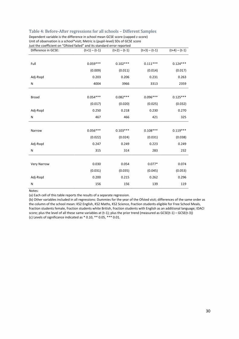
30

Table 4: Before-After regressions for all schools – Different Samples Dependent variable is the difference in school mean GCSE score (capped z-score) Unit of observation is a school*visit; Metric is (pupil-level) SDs of GCSE score Just the coefficient on “Ofsted failed” and its standard error reported

Difference in GCSE: (t+1) – (t-1) (t+2) – (t-1) (t+3) – (t-1) (t+4) – (t-1)

Full 0.059*** 0.102*** 0.111*** 0.124***

(0.009) (0.011) (0.014) (0.017)

Adj-Rsqd 0.203 0.206 0.231 0.263

N 4004 3966 3313 2359

Broad 0.054*** 0.082*** 0.096*** 0.125***

(0.017) (0.020) (0.025) (0.032)

Adj-Rsqd 0.250 0.218 0.230 0.270

N 467 466 421 325

Narrow 0.056*** 0.103*** 0.108*** 0.119***

(0.022) (0.024) (0.031) (0.038)

Adj-Rsqd 0.247 0.249 0.223 0.249

N 315 314 283 232

Very Narrow 0.030 0.054 0.077* 0.074

(0.031) (0.035) (0.045) (0.053)

Adj-Rsqd 0.200 0.215 0.262 0.296

N 156 156 139 119

Notes: (a) Each cell of this table reports the results of a separate regression. (b) Other variables included in all regressions: Dummies for the year of the Ofsted visit; differences of the same order as the column of the school mean: KS2 English, KS2 Maths, KS2 Science, fraction students eligible for Free School Meals, fraction students female, fraction students white British, fraction students with English as an additional language; IDACI score; plus the level of all these same variables at (t-1); plus the prior trend (measured as GCSE(t-1) – GCSE(t-3)) (c) Levels of significance indicated as * 0.10, ** 0.05, *** 0.01.

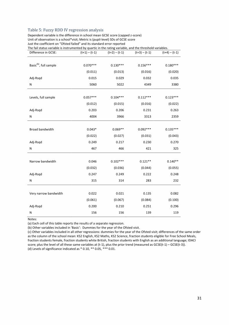
31

Table 5: Fuzzy RDD IV regression analysis Dependent variable is the difference in school mean GCSE score (capped z-score) Unit of observation is a school*visit; Metric is (pupil-level) SDs of GCSE score Just the coefficient on “Ofsted failed” and its standard error reported The fail status variable is instrumented by quartic in the rating variable, and the threshold variables.

Difference in GCSE: (t+1) – (t-1) (t+2) – (t-1) (t+3) – (t-1) (t+4) – (t-1)

Basic(b)

, full sample 0.070*** 0.130*** 0.156*** 0.180***

(0.011) (0.013) (0.016) (0.020)

Adj-Rsqd 0.015 0.029 0.032 0.035

N 5060 5022 4349 3380

Levels, full sample 0.057*** 0.104*** 0.112*** 0.123***

(0.012) (0.015) (0.016) (0.022)

Adj-Rsqd 0.203 0.206 0.231 0.263

N 4004 3966 3313 2359

Broad bandwidth 0.043* 0.069** 0.092*** 0.135***

(0.022) (0.027) (0.031) (0.043)

Adj-Rsqd 0.249 0.217 0.230 0.270

N 467 466 421 325

Narrow bandwidth 0.046 0.102*** 0.121** 0.140**

(0.032) (0.036) (0.044) (0.055)

Adj-Rsqd 0.247 0.249 0.222 0.248

N 315 314 283 232

Very narrow bandwidth 0.022 0.021 0.135 0.082

(0.061) (0.067) (0.084) (0.100)

Adj-Rsqd 0.200 0.210 0.251 0.296

N 156 156 139 119

Notes: (a) Each cell of this table reports the results of a separate regression. (b) Other variables included in ‘Basic’: Dummies for the year of the Ofsted visit. (c) Other variables included in all other regressions: dummies for the year of the Ofsted visit; differences of the same order as the column of the school mean: KS2 English, KS2 Maths, KS2 Science, fraction students eligible for Free School Meals, fraction students female, fraction students white British, fraction students with English as an additional language; IDACI score; plus the level of all these same variables at (t-1), plus the prior trend (measured as GCSE(t-1) – GCSE(t-3)). (d) Levels of significance indicated as * 0.10, ** 0.05, *** 0.01.

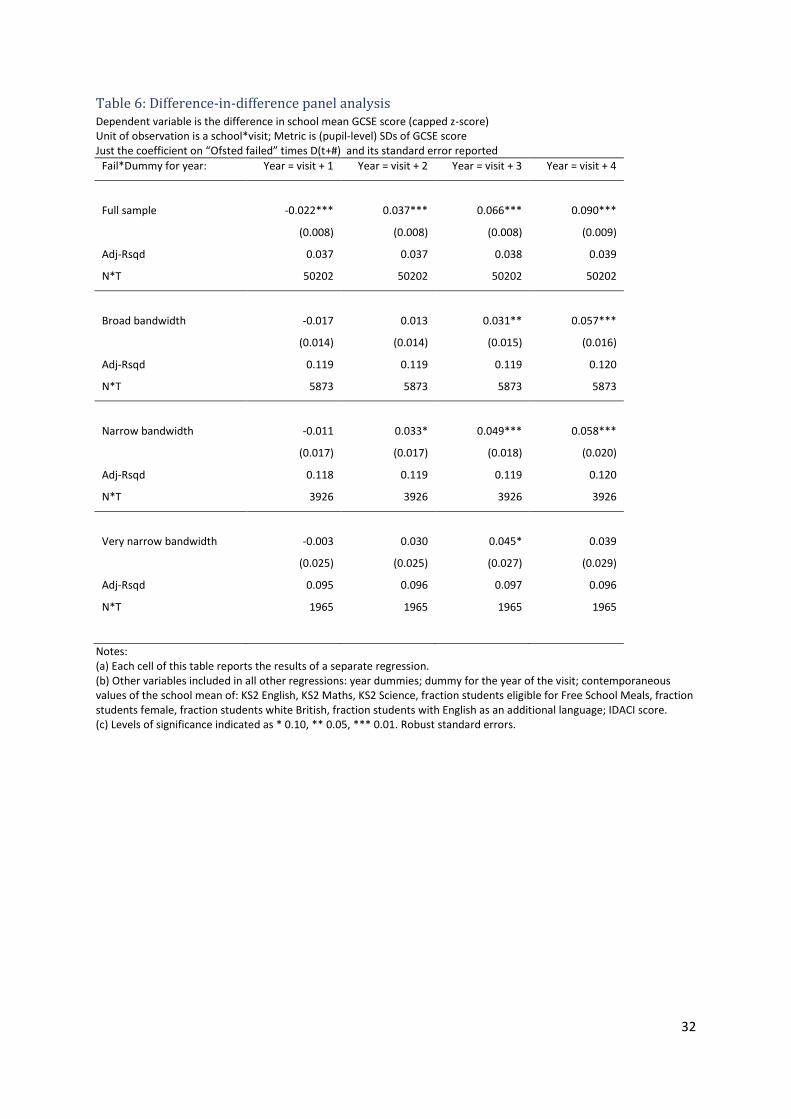
32

Table 6: Difference-in-difference panel analysis Dependent variable is the difference in school mean GCSE score (capped z-score) Unit of observation is a school*visit; Metric is (pupil-level) SDs of GCSE score Just the coefficient on “Ofsted failed” times D(t+#) and its standard error reported

Fail*Dummy for year: Year = visit + 1 Year = visit + 2 Year = visit + 3 Year = visit + 4

Full sample -0.022*** 0.037*** 0.066*** 0.090***

(0.008) (0.008) (0.008) (0.009)

Adj-Rsqd 0.037 0.037 0.038 0.039

N*T 50202 50202 50202 50202

Broad bandwidth -0.017 0.013 0.031** 0.057***

(0.014) (0.014) (0.015) (0.016)

Adj-Rsqd 0.119 0.119 0.119 0.120

N*T 5873 5873 5873 5873

Narrow bandwidth -0.011 0.033* 0.049*** 0.058***

(0.017) (0.017) (0.018) (0.020)

Adj-Rsqd 0.118 0.119 0.119 0.120

N*T 3926 3926 3926 3926

Very narrow bandwidth -0.003 0.030 0.045* 0.039

(0.025) (0.025) (0.027) (0.029)

Adj-Rsqd 0.095 0.096 0.097 0.096

N*T 1965 1965 1965 1965

Notes: (a) Each cell of this table reports the results of a separate regression. (b) Other variables included in all other regressions: year dummies; dummy for the year of the visit; contemporaneous values of the school mean of: KS2 English, KS2 Maths, KS2 Science, fraction students eligible for Free School Meals, fraction students female, fraction students white British, fraction students with English as an additional language; IDACI score. (c) Levels of significance indicated as * 0.10, ** 0.05, *** 0.01. Robust standard errors.

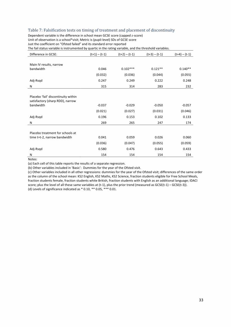
33

Table 7: Falsification tests on timing of treatment and placement of discontinuity Dependent variable is the difference in school mean GCSE score (capped z-score) Unit of observation is a school*visit; Metric is (pupil-level) SDs of GCSE score Just the coefficient on “Ofsted failed” and its standard error reported The fail status variable is instrumented by quartic in the rating variable, and the threshold variables.

Difference in GCSE: (t+1) – (t-1) (t+2) – (t-1) (t+3) – (t-1) (t+4) – (t-1)

Main IV results, narrow bandwidth 0.046 0.102*** 0.121** 0.140**

(0.032) (0.036) (0.044) (0.055)

Adj-Rsqd 0.247 0.249 0.222 0.248

N 315 314 283 232

Placebo ‘fail’ discontinuity within satisfactory (sharp RDD), narrow bandwidth -0.037 -0.029 -0.050 -0.057

(0.021) (0.027) (0.031) (0.046)

Adj-Rsqd 0.196 0.153 0.102 0.133

N 269 265 247 174

Placebo treatment for schools at time t=t-2, narrow bandwidth 0.041 0.059 0.026 0.060

(0.036) (0.047) (0.055) (0.059)

Adj-Rsqd 0.580 0.476 0.643 0.433

N 154 154 154 154

Notes: (a) Each cell of this table reports the results of a separate regression. (b) Other variables included in ‘Basic’: Dummies for the year of the Ofsted visit. (c) Other variables included in all other regressions: dummies for the year of the Ofsted visit; differences of the same order as the column of the school mean: KS2 English, KS2 Maths, KS2 Science, fraction students eligible for Free School Meals, fraction students female, fraction students white British, fraction students with English as an additional language; IDACI score; plus the level of all these same variables at (t-1), plus the prior trend (measured as GCSE(t-1) – GCSE(t-3)). (d) Levels of significance indicated as * 0.10, ** 0.05, *** 0.01.

34

Table 8: Fuzzy RDD IV regression analysis, different outcome variables, Narrow sample Dependent variable is the difference in school mean of various outcome measures Unit of observation is a school*visit; Metric is (pupil-level) SDs for row 1, fraction for row 2, and mean point score (from 1 to 8) for rows 3 and 4. Just the coefficient on “Ofsted failed” and its standard error reported. The fail status variable is instrumented by the rating variable.

Difference in GCSE: (t+1) – (t-1) (t+2) – (t-1) (t+3) – (t-1) (t+4) – (t-1)

Capped mean GCSE score 0.046 0.102*** 0.121** 0.140**

(0.032) (0.036) (0.044) (0.055)

Adj-Rsqd 0.247 0.249 0.222 0.248

N 315 314 283 232

Fraction of pupils achieving

at least 5 A*-C grades

0.024 0.037* 0.050** 0.058**

(0.019) (0.021) (0.025) (0.029)

Adj-Rsqd 0.237 0.275 0.226 0.272

N 315 314 283 232

Mean Maths GCSE score 0.139** 0.164** 0.141* 0.094

(0.062) (0.068) (0.079) (0.082)

Adj-Rsqd 0.406 0.253 0.221 0.272

N 315 314 283 232

Mean English GCSE score 0.146** 0.114* 0.106 0.074

(0.059) (0.064) (0.074) (0.081)

Adj-Rsqd 0.279 0.250 0.239 0.276

N 315 314 283 232

Notes: (a) Each cell of this table reports the results of a separate regression. (b) Other variables included in all other regressions: dummies for the year of the Ofsted visit; differences of the same order as the column of the school mean: KS2 English, KS2 Maths, KS2 Science, fraction students eligible for Free School Meals, fraction students female, fraction students white British, fraction students with English as an additional language; IDACI score; plus the level of all these same variables at (t-1); plus the prior trend (measured as GCSE(t-1) – GCSE(t-3)). (d) Levels of significance indicated as * 0.10, ** 0.05, *** 0.01.

35

Table 9: Analysis of marginal pupils versus others, narrow sample Dependent variable is the difference in school mean of various outcome measures Unit of observation is a school*visit; Metric is (pupil-level) SDs for row 1, fraction for row 2, and mean point score (from 1 to 8) for rows 3 and 4. Just the coefficient on “Ofsted failed” and its standard error reported. The fail status variable is instrumented by the rating variable.

Difference in GCSE: (t+1) – (t-1) (t+2) – (t-1) (t+3) – (t-1) (t+4) – (t-1)

Capped mean GCSE score

Lower ability students 0.010 0.075* 0.117** 0.118*

(0.037) (0.045) (0.048) (0.062)

Marginal students 0.082* 0.093* 0.113** 0.157**

(0.044) (0.048) (0.053) (0.064)

Higher ability students 0.085* 0.106** 0.095* 0.216***

(0.044) (0.050) (0.055) (0.069)

5+ A*-C GCSE score

Lower ability students -0.017 0.014 0.030 0.049

(0.025) (0.031) (0.035) (0.046)

Marginal students 0.055** 0.043 0.061** 0.071**

(0.028) (0.030) (0.029) (0.030)

Higher ability students 0.028* 0.032* 0.043*** 0.058***

(0.015) (0.017) (0.016) (0.016)

Maths GCSE

Lower ability students 0.023 0.058 0.052 -0.028

(0.066) (0.079) (0.087) (0.105)

Marginal students 0.211** 0.136 0.136 0.112

(0.082) (0.086) (0.085) (0.100)

Higher ability students 0.151** 0.072 0.075 0.161

(0.073) (0.089) (0.082) (0.105)

English GCSE

Lower ability students 0.086 0.068 0.046 -0.044

(0.071) (0.082) (0.089) (0.101)

Marginal students 0.211*** 0.103 0.121 0.086

(0.066) (0.068) (0.076) (0.088)

Higher ability students 0.098 -0.010 0.034 0.083

(0.071) (0.076) (0.087) (0.097)

N 312 311 280 229

Notes: (a) Each cell of this table reports the results of a separate regression. (b) Other variables included in all other regressions: dummies for the year of the Ofsted visit; differences of the same order as the column of the school mean: KS2 English, KS2 Maths, KS2 Science, fraction students eligible for Free School Meals, fraction students female, fraction students white British, fraction students with English as an additional language; IDACI score; plus the level of all these same variables at (t-1). (c) Levels of significance indicated as * 0.10, ** 0.05, *** 0.01.

36

Table 10: Analysis of change in pupil intake Dependent variable is the difference in school mean of various measures of the school intake Unit of observation is a school*visit; Metric is number of pupils in row 1, the mean points score in row 2, and the proportion in row 3. Just the coefficient on “Ofsted failed” and its standard error reported. The fail status variable is instrumented by the rating variable.

Difference in year 7 metric: (t+1) – (t-1) (t+2) – (t-1) (t+3) – (t-1) (t+4) – (t-1)

Number of pupils in cohort -4.493 -4.977 2.265 -0.532

(5.003) (6.503) (6.896) (8.926)

Adj-Rsqd 0.032 -0.010 -0.006 0.009

N 313 308 280 225

Mean KS2 score 0.027 -0.003 -0.012 -0.011

(0.024) (0.027) (0.029) (0.037)

Adj-Rsqd 0.142 0.095 0.103 0.100

N 313 308 280 225

FSM proportion -0.011 -0.009 -0.025 -0.002

(0.013) (0.013) (0.016) (0.012)

Adj-Rsqd 0.323 0.345 0.369 0.485

N 313 308 280 225

Notes: (a) Each cell of this table reports the results of a separate regression. (b) Other variables included in all other regressions: dummies for the year of the Ofsted visit. (c) Levels of significance indicated as * 0.10, ** 0.05, *** 0.01.

37

Figures

Figure 1: RDD assignment variable: Fraction failing and density

Note: Bandwidths shown are Broad, Narrow and Very Narrow samples.

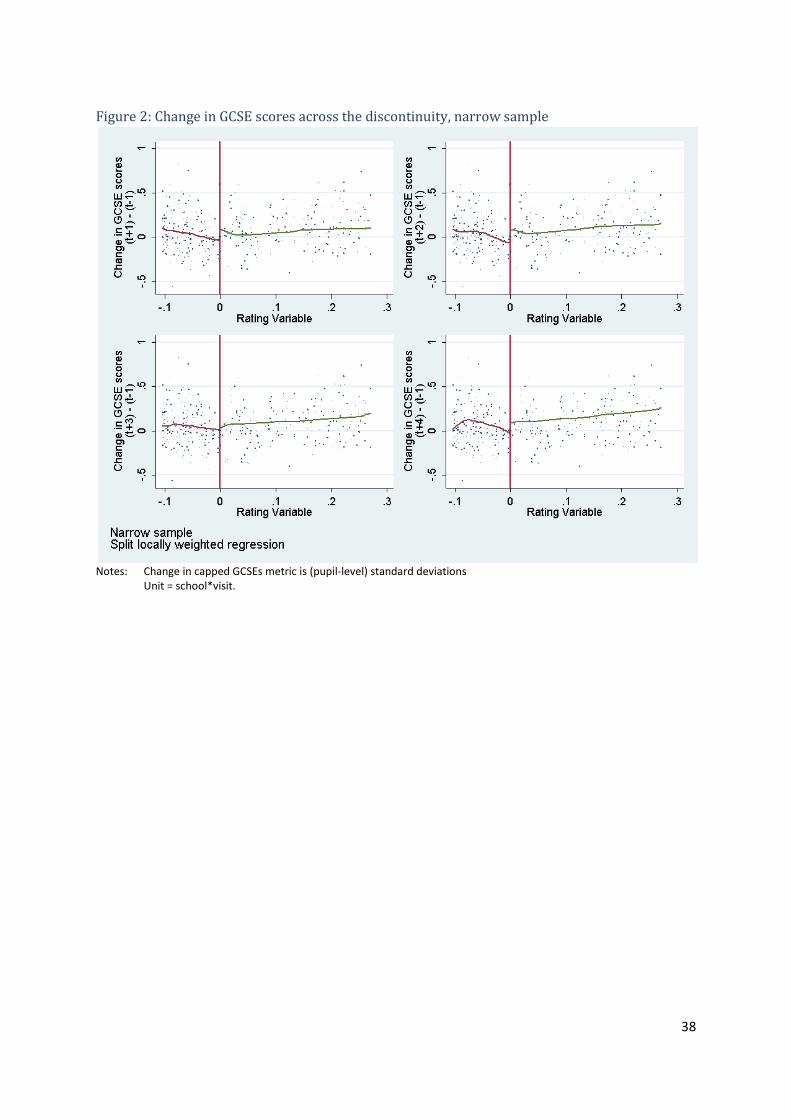
38

Figure 2: Change in GCSE scores across the discontinuity, narrow sample

Notes: Change in capped GCSEs metric is (pupil-level) standard deviations

Unit = school*visit.

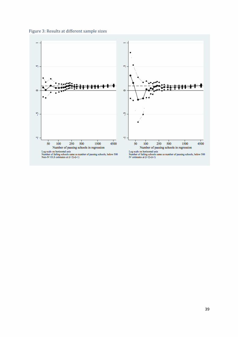
39

Figure 3: Results at different sample sizes

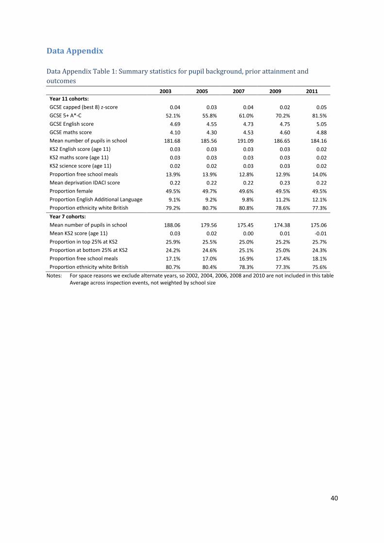
40

Data Appendix

Data Appendix Table 1: Summary statistics for pupil background, prior attainment and

outcomes 2003 2005 2007 2009 2011

Year 11 cohorts: GCSE capped (best 8) z-score 0.04 0.03 0.04 0.02 0.05

GCSE 5+ A*-C 52.1% 55.8% 61.0% 70.2% 81.5%

GCSE English score 4.69 4.55 4.73 4.75 5.05

GCSE maths score 4.10 4.30 4.53 4.60 4.88

Mean number of pupils in school 181.68 185.56 191.09 186.65 184.16

KS2 English score (age 11) 0.03 0.03 0.03 0.03 0.02

KS2 maths score (age 11) 0.03 0.03 0.03 0.03 0.02

KS2 science score (age 11) 0.02 0.02 0.03 0.03 0.02

Proportion free school meals 13.9% 13.9% 12.8% 12.9% 14.0%

Mean deprivation IDACI score 0.22 0.22 0.22 0.23 0.22

Proportion female 49.5% 49.7% 49.6% 49.5% 49.5%

Proportion English Additional Language 9.1% 9.2% 9.8% 11.2% 12.1%

Proportion ethnicity white British 79.2% 80.7% 80.8% 78.6% 77.3%

Year 7 cohorts: Mean number of pupils in school 188.06 179.56 175.45 174.38 175.06

Mean KS2 score (age 11) 0.03 0.02 0.00 0.01 -0.01

Proportion in top 25% at KS2 25.9% 25.5% 25.0% 25.2% 25.7%

Proportion at bottom 25% at KS2 24.2% 24.6% 25.1% 25.0% 24.3%

Proportion free school meals 17.1% 17.0% 16.9% 17.4% 18.1%

Proportion ethnicity white British 80.7% 80.4% 78.3% 77.3% 75.6%

Notes: For space reasons we exclude alternate years, so 2002, 2004, 2006, 2008 and 2010 are not included in this table Average across inspection events, not weighted by school size

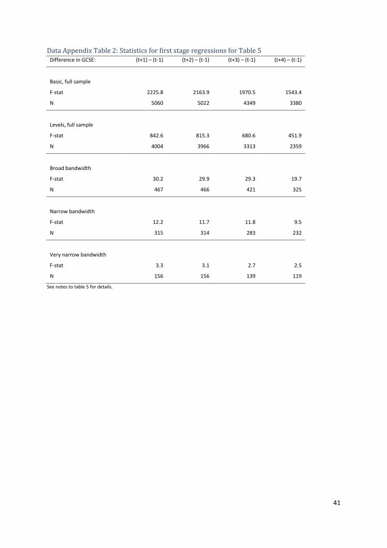
41

Data Appendix Table 2: Statistics for first stage regressions for Table 5 Difference in GCSE: (t+1) – (t-1) (t+2) – (t-1) (t+3) – (t-1) (t+4) – (t-1)

Basic, full sample

F-stat 2225.8 2163.9 1970.5 1543.4

N 5060 5022 4349 3380

Levels, full sample

F-stat 842.6 815.3 680.6 451.9

N 4004 3966 3313 2359

Broad bandwidth

F-stat 30.2 29.9 29.3 19.7

N 467 466 421 325

Narrow bandwidth

F-stat 12.2 11.7 11.8 9.5

N 315 314 283 232

Very narrow bandwidth

F-stat 3.3 3.1 2.7 2.5

N 156 156 139 119

See notes to table 5 for details.

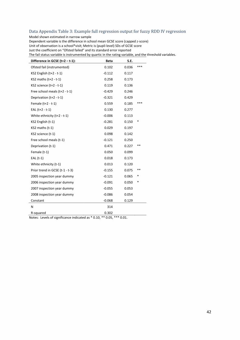
42

Data Appendix Table 3: Example full regression output for fuzzy RDD IV regression Model shown estimated in narrow sample Dependent variable is the difference in school mean GCSE score (capped z-score) Unit of observation is a school*visit; Metric is (pupil-level) SDs of GCSE score Just the coefficient on “Ofsted failed” and its standard error reported The fail status variable is instrumented by quartic in the rating variable, and the threshold variables.

Difference in GCSE (t+2 – t-1): Beta S.E.

Ofsted fail (instrumented) 0.102 0.036 ***

KS2 English (t+2 - t-1) -0.112 0.117

KS2 maths (t+2 - t-1) 0.258 0.173

KS2 science (t+2 - t-1) 0.119 0.136

Free school meals (t+2 - t-1) -0.429 0.246

Deprivation (t+2 - t-1) -0.321 0.429

Female (t+2 - t-1) 0.559 0.185 ***

EAL (t+2 - t-1) 0.130 0.277

White ethnicity (t+2 - t-1) -0.006 0.113

KS2 English (t-1) -0.281 0.150 *

KS2 maths (t-1) 0.029 0.197

KS2 science (t-1) 0.098 0.142

Free school meals (t-1) -0.121 0.250

Deprivation (t-1) 0.471 0.227 **

Female (t-1) 0.050 0.099

EAL (t-1) 0.018 0.173

White ethnicity (t-1) 0.013 0.120

Prior trend in GCSE (t-1 - t-3) -0.155 0.075 **

2005 inspection year dummy -0.121 0.065 *

2006 inspection year dummy -0.091 0.050 *

2007 inspection year dummy -0.055 0.053

2008 inspection year dummy -0.086 0.054

Constant -0.068 0.129

N 314

R-squared 0.302

Notes: Levels of significance indicated as * 0.10, ** 0.05, *** 0.01.