Embed Size (px)
Citation preview
How sensitive is regional poverty measurement
in Latin America to the value of the poverty line?
R. Andrés Castañeda Santiago Garriga†
Leonardo Gasparini§ Leonardo R. Lucchetti‡
Daniel Valderrama††
March 20, 2018
Abstract
This paper contributes to the methodological literature on the estimation of international
poverty lines for Latin America based on the official poverty lines chosen by the Latin
American governments and commonly used in the public debate. The paper exploits a
comprehensive data set of 86 up-to-date official extreme and total urban poverty lines
across 18 countries in Latin America, as well as the recently updated values of the national
purchasing power parity conversion factors from the 2011 International Comparison
Program, and a set of harmonized household surveys. By using 3 and 6 US dollars per
person a day at 2011 PPP as the extreme and total poverty lines for Latin America, this
paper illustrates the sensitiveness of poverty rates to changes of the values of the poverty
lines as a result of the recent update of the PPP values, the period of reference, and the
relative cost of living across the countries in the region. The poverty lines with the 2011
PPP values lead to an increase in total poverty rates in Latin America when compared to
the 2005 PPP values, while they leave the extreme poverty rate unaffected. In general,
country-specific poverty rankings remain fairly stable to the values of the poverty lines
selected.
JEL classification: I3, I32, D6, E31, F01
Keywords: poverty, poverty lines, purchasing power parity, Latin America
We are grateful to Oscar Calvo-Gonzalez, Liliana Sousa, Maria Ana Lugo, Thiago Scot, Ankush Khullar, and participants at the
World Bank “Summer Initiative on Research on Poverty Inequality and Gender”; the Global Poverty Working Group within the
World Bank whose suggestions greatly improved earlier drafts of the paper; and the 21st Annual LACEA meeting in Medellin.
All remaining errors are ours. World Bank. E-mail: [email protected] † Paris School of Economics - École des hautes études en sciences sociales. E-mail: [email protected] § Centro de Estudios Distributivos, Laborales, y Sociales (CEDLAS) at the Universidad Nacional de La Plata (UNLP) and
CONICET. E-mail: [email protected] ‡ World Bank. E-mail: [email protected] †† Georgetown University – Department of Economics. E-mail: [email protected]
2
1 Introduction
The international comparison of poverty measures is a central tool for development research.
Comparing the performance of different countries in terms of poverty reduction is informative
about the effect of structural characteristics, shocks, and policies on the well-being of the most
vulnerable. Naturally, to carry out international comparisons, poverty should be measured
consistently across countries. Unfortunately, at least for the purpose of research in international
development, there is not a global protocol to measure poverty at the national level. In practice,
poverty measurement differs from country to country in many respects, including: (i) the
methodology to estimate the poverty line (e.g., relative vs. absolute lines, the minimum amount
of calories, the choice of the reference group, or the procedure to go from extreme to total
poverty lines); (ii) the choice of the individual welfare measure (e.g., income vs. consumption);
(iii) the construction of the welfare aggregate (e.g., items included in the income or consumption
variable or the treatment of implicit rent of own housing); (iv) the design of surveys (e.g.,
differences in questionnaire design); and (v) many other adjustments and considerations (e.g.,
adult equivalent scales vs. per capita values, economies of scale, and regional prices).
Consequently, the comparison of official poverty estimates across countries is generally
misleading. Thus, any attempt to generate meaningful poverty comparisons and to aggregate
national poverty indicators into regional and global ones requires a standardized measure of
household welfare and a common poverty line.
Ideally, the common poverty line should be constructed by agreeing on a bundle of
goods, and computing the market price of that same bundle in all the countries. This undertaking
however has proved difficult to materialize since it requires a high degree of international
coordination. In Latin America, the United Nations, through its regional agency ECLAC, has
made some inroads into that goal, but still countries in the region continue measuring poverty
with substantial heterogeneity.
A body of research has proposed some alternative methods to obtain standardized
measures of monetary poverty that are comparable across countries and independent of the
official methodologies applied in each country. The most widespread accepted initiative is to
define an international poverty line in US dollars and “translate” this value into local currency
units using consumption purchasing power parity (PPP) exchange rates, computed by the
International Comparison Program (ICP), a large project on price comparisons around the world.
The proposal requires setting a value in dollars for the international poverty line. To some
extent this should not be an issue, since it is well known in the development literature that lines
are arbitrary cultural constructions, given that there are not discontinuities in any well-being
3
indicator (Deaton 1997). A thorough poverty analysis should not be confined to a single line, but
instead should consider a set of poverty lines, or better, check stochastic dominance conditions.
However, it has proved useful in the policy debate, and in the development literature, to define
some “focal” values for the poverty lines. These agreed values, although still arbitrary, are
helpful to simplify the discussions.
The seminal work by Ravallion, Datt, and van de Walle (1991) proposed one of the first
global extreme poverty lines at $1.01 (rounded to $1) per person per day at 1990 PPPs based on
1985 prices surveyed by the ICP.1 This global extreme poverty line corresponded to the average
of the poverty lines of the eight most deprived economies in the world and became the
foundation for the United Nations’ first Millennium Development Goals of halving the
proportion of people with incomes lower than $1 a day between 1990 and 2015. This line was
then revised by Chen and Ravallion (2001) to $1.08 per person per day at 1993 PPPs, and by
Ravallion, Chen, and Sangraula (2009) to $1.25 per person per day at 2005 PPPs, the latter of
which is known today as the Global Extreme Poverty Line and is computed as the average of the
poverty lines of the 15 poorest countries in the world. Recently, Jolliffe and Prydz (2015)
proposed an update of the Global Extreme Poverty Line which resulted in a poverty line of $1.92
per person per day in 2011 PPPs, while Ferreira et al. (2016) calculated it as $1.88 (rounded to
1.90) per person per day.
The Global Extreme Poverty Line frequently used for international poverty comparisons
in the developing world was derived from poverty lines set in the poorest Sub-Sahara African
countries; therefore, they have limited applicability in Latin America, a region composed mostly
of urbanized middle-income economies. The share of the population under that line is lower than
5 percent in the region. Even the $2 per person per day poverty line, commonly used for middle-
income countries, is “too low” compared with the lines officially chosen by the Latin American
countries and used in the policy debate.2 Consequently, these international lines fail to be “focal”
and become irrelevant for all local discussions.
1 Ahluwalia, Carter, and Chenery (1979) used India’s poverty line to estimate poverty at a global level based on the
1975 PPPs. This was the first attempt to measure global poverty, though it was based on income and consumption
data from only 25 countries in the world (Ferreira et al. 2016).
2 Most countries in the region officially use two poverty lines: an extreme (food) and a total (food and non-food)
poverty line. Countries estimate their extreme poverty lines as the lack of per capita income required to access a
basic food basket and expand them to non-food components using the Orshansky coefficient (Orshansky 1963).
4
Given this problem, many researchers and institutions like the World Bank, the Inter-
American Development Bank (IADB), and ECLAC3 use for Latin America an extreme and total
poverty line of $2.5 and $4 per person per day in 2005 PPPs, respectively. Although there is not
a formal document supporting this choice, Gasparini et al. (2013) report that these lines were
close to the unweighted median of the poverty lines for the main urban areas of a sample of
countries in 2005 (the sample excludes Brazil, the most populated country in the region).
In this paper, we provide inputs for deriving “focal” regional poverty lines by considering
the US$ value of the extreme and total poverty lines officially chosen by the Latin American
countries, and used in their own poverty and social policy debates. Besides providing a detailed
description of the methodology, we improve the computations on several grounds. In particular,
we exploit a unique data set of 86 official subnational urban poverty lines across 18 Latin
American countries, as well as the recent 2011 PPPs from the ICP. We compute different
weighted and unweighted statistics and carry out a robustness analysis of the results.
As far as we know, this study is the first one that explicitly documents the calculation of
regional extreme and total poverty lines. Our proposal has some strengths compared to lines
computed by other studies in the developing world. First, the proposed lines are based on a
comprehensive list of all countries for which up-to-date data on official poverty lines are
available (18 countries representing roughly 85.3 percent of Latin America’s population in 2011
and almost all urban population of the region). As such, any existing bias in the estimation of the
value of the regional poverty lines that results from excluding certain countries is likely to be
relatively small.4 Second, using up-to-date information from National Statistical Offices (NSO)
in Latin America on poverty lines used to estimate official extreme and moderate poverty
numbers in every country can be considered more transparent and easier to communicate to
governments in the region. Third, the method proposed in this paper is relatively simple and easy
to replicate, which is key to ensure credibility to the process (Ferreira et al. 2016). Fourth, this
paper uses subnational official urban poverty lines when available, which accounts for regional
disparities in the standard of living within countries and allows for the replication of countries’
official poverty estimates. Finally, by using the most up-to-date poverty lines from NSOs in
3 López-Calva and Ortiz-Juarez (2014); Gasparini, Cicowiez, and Escudero (2013); Ferreira et al. (2012); World
Bank (2015); World Bank (2014); World Bank (2013); World Bank (2011); Stampini et al. (2015), among others.
4 Deaton (2010) argues that changes in the composition of the 15 countries used by Ravallion et al. (1991) result in
significant changes in the value of the poverty line and the count of the poor worldwide (Jolliffe and Prydz 2015).
5
Latin America, our approach is less sensitive to changes in Consumer Price Index (CPI) data
(Chen and Ravallion 2010; Jolliffe and Prydz 2015).
Depending on the specification chosen, the paper estimates the set of extreme and total
poverty lines to be approximately $2.5 to $3.2, and $5.3 to $6.8 per person per day at 2011 PPP
values, respectively. We then apply these lines to the distribution of household per capita
income, which is standardized under the SEDLAC project, a joint initiative of the World Bank
and the Center for Distributional Labor and Social Studies (CEDLAS) at Universidad Nacional
de La Plata (UNLP) in Argentina,5 in all Latin American countries for which microdata are
available. Depending on the regional poverty line selected, we find that approximately 7 percent
to 11 percent of individuals were extremely poor in 2013, while approximately 24 to 35 percent
of the population were living with a per capita income lower than the total poverty line during
the same year.
For the sake of illustration, we use the 3 and 6 US dollars per person a day at 2011 PPP
as poverty lines for Latin America. Then, we estimate the sensitivity of the poverty rates to
changes of the value of the regional poverty lines when changing the value of the PPP, the period
of reference, and the relative cost of living across the countries in the region.
The rest of the document is organized as follows. Section 2 outlines the methodology and
brings together the various sources of information used. Section 3 presents the results for the
poverty lines, whereas section 4 reports the resulting headcount ratios. In section 5 we carry out a
simulation exercise that quantifies the sources of differences between the poverty estimates
under our proposal and those arising from the lines that are currently used by The World Bank
and some researchers. Section 6 ends with some concluding remarks.
2 Methodology and data
Given the large heterogeneities across geographical areas, Latin American governments typically
measure poverty by setting poverty lines at the subnational level. We propose to derive
international aggregate poverty lines for Latin America from these subnational official poverty
lines. Although the proposal is rather straightforward, some notation may clarify it. Define zrp as
the official poverty line for the subnational area r in country p expressed in a common currency.
5 CEDLAS and World Bank (2015).
6
As usual in the international studies, we express all lines in US dollars per person per day at
purchasing power parity (PPP) values.
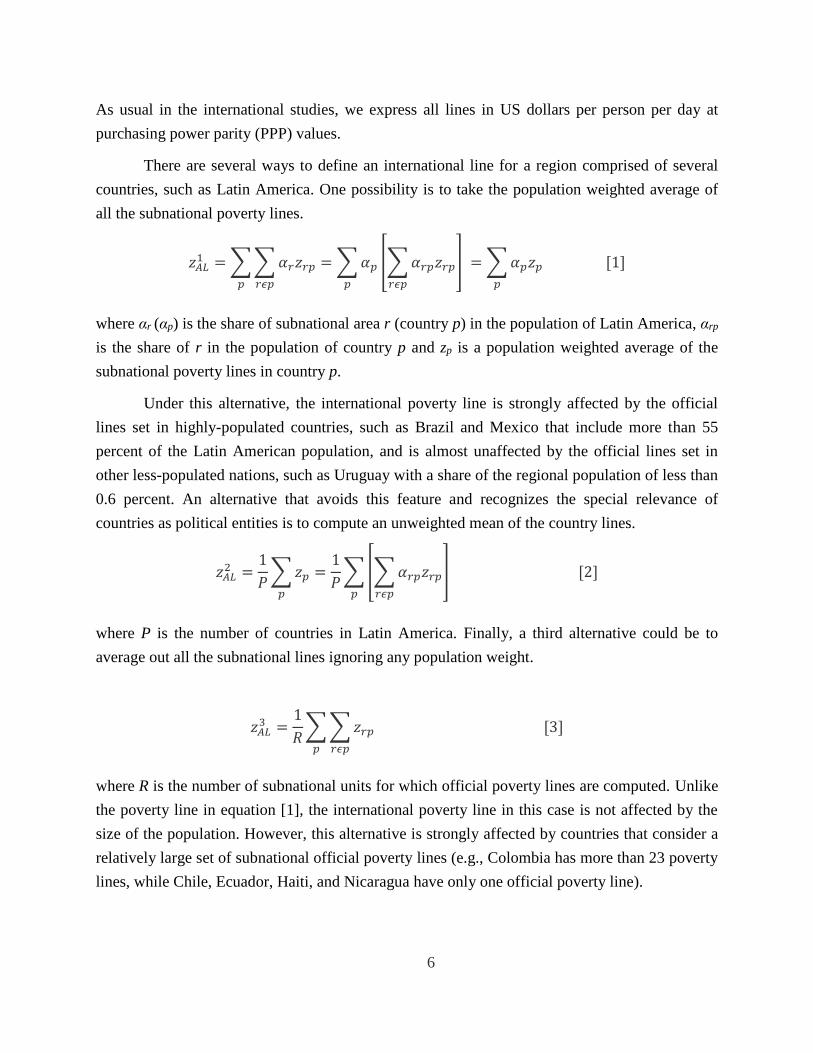
There are several ways to define an international line for a region comprised of several
countries, such as Latin America. One possibility is to take the population weighted average of
all the subnational poverty lines.
𝑧𝐴𝐿1 = ∑ ∑ 𝛼𝑟𝑧𝑟𝑝
𝑟𝜖𝑝𝑝
= ∑ 𝛼𝑝 [∑ 𝛼𝑟𝑝𝑧𝑟𝑝
𝑟𝜖𝑝
]
𝑝
= ∑ 𝛼𝑝𝑧𝑝
𝑝
[1]
where αr (αp) is the share of subnational area r (country p) in the population of Latin America, αrp
is the share of r in the population of country p and zp is a population weighted average of the
subnational poverty lines in country p.
Under this alternative, the international poverty line is strongly affected by the official
lines set in highly-populated countries, such as Brazil and Mexico that include more than 55
percent of the Latin American population, and is almost unaffected by the official lines set in
other less-populated nations, such as Uruguay with a share of the regional population of less than
0.6 percent. An alternative that avoids this feature and recognizes the special relevance of
countries as political entities is to compute an unweighted mean of the country lines.
𝑧𝐴𝐿2 =
1
𝑃∑ 𝑧𝑝
𝑝
=1
𝑃∑ [∑ 𝛼𝑟𝑝𝑧𝑟𝑝
𝑟𝜖𝑝
] [2]
𝑝
where P is the number of countries in Latin America. Finally, a third alternative could be to
average out all the subnational lines ignoring any population weight.
𝑧𝐴𝐿3 =
1
𝑅∑ ∑ 𝑧𝑟𝑝
𝑟𝜖𝑝
𝑝
[3]
where R is the number of subnational units for which official poverty lines are computed. Unlike
the poverty line in equation [1], the international poverty line in this case is not affected by the
size of the population. However, this alternative is strongly affected by countries that consider a
relatively large set of subnational official poverty lines (e.g., Colombia has more than 23 poverty
lines, while Chile, Ecuador, Haiti, and Nicaragua have only one official poverty line).
7
Equations [1] to [3] illustrate the different alternatives with a measure of central
tendency: the mean. In the empirical implementation, we also compute the median for each case,
which has the convenient property of being less sensitive to extreme values.
To implement the methodology, we use three different data sets: (i) country-specific
official poverty lines from National Statistical Offices, (ii) the PPPs from the 2011 ICP round,
and (iii) household per capita income distribution from harmonized household surveys.
2.1 Country-specific official poverty lines
We make use of data on subnational official extreme and total poverty lines that correspond to
closest to the last 2011 PPP round. These lines were obtained from NSOs or governmental
agencies from 18 countries in Latin America: Argentina, Bolivia, Brazil,6 Chile, Colombia,
Costa Rica, the Dominican Republic, Ecuador, El Salvador, Guatemala, Haiti, Honduras,
Mexico, Nicaragua, Panama, Paraguay, Peru, and Uruguay.7 We collect more than 80
subnational urban8 poverty lines, accounting for regional disparities within countries by
capturing subnational heterogeneities in the standard of living.9
The level of subnational disaggregation varies from country to country. For some
countries poverty lines are determined at the level of cities (e.g., Colombia), while for others
they are determined at the regional level (e.g., Brazil). In some few cases, there is just one line at
the national level (e.g., Nicaragua). Almost all poverty lines are in per capita terms; the only
exceptions are Argentina where poverty lines also consider household composition and Uruguay
where the non-food component of the poverty line accounts for economies of scale.
6 The Brazilian case is different from the rest; the country does not have an official poverty line. For the purpose of
this paper, we use subnational poverty lines calculated by Institute for Applied Economic Research (IPEA, for its
acronym in Portuguese) updated on a yearly bases based on the CPI (IPEA 2014).
7 Cuba and Venezuela are not included in this study due to the lack of microdata from SEDLAC project in both
countries and the lack of poverty lines in the case of Cuba. The estimation of the international poverty lines is
robust to the inclusion of Venezuela.
8 See section 2.3 for the reason we restrict the analysis to urban poverty lines.
9 The pioneering work of Ravallion, Datt, and van de Walle (1991) gathered a compilation of 33 non-official
national poverty lines for the whole world, while Ravallion, Chen, and Sangraula (2009) used data on 88 poverty
lines extracted from the World Bank’s program of country Poverty Assessments that have been carried out since
1990 worldwide. In a recent paper Jolliffe and Prydz (2016) compute implicit national poverty lines from
combining official poverty headcounts, as reported in World Bank Poverty Assessments, with the corresponding
consumption and income distributions from the World Bank’s PovcalNet database. One caveat of this exercise is
that the combination of official poverty rates with unofficial harmonized micro-data sets from PovcalNet may
result in poverty lines that deviate from the official ones, which is the case for Latin American countries.
8
2.2 Purchasing power parity exchange rates
In order to compare the standard of living of households across countries in Latin America,
household welfare needs to be expressed in common units. Pursuing that purpose, the ICP
launched in May 2014 an update of its PPP data based on information of goods and services for
almost every country in the world.10 The updated PPP data allow for the comparison of
household welfare across countries by providing a real exchange rate from local currency to US
dollar in a particular year—2011 in this case.11 The 2011 update of PPPs increased its coverage,
collecting prices from 199 countries in the world, up from 146 in the previous update, and
included several methodological and operational improvements with respect to 2005.12
Why not use exchange rates to express welfare measures in common units across countries?
The main difference between the PPP data and the nominal exchange rate is that the former is
created as an index of prices of the same basket of goods in the same period, whereas the latter is
the price of a local currency in terms of a foreign one (i.e., the rate by which both currencies are
exchanged). The nominal exchange rate reflects prices of only tradable goods and, hence, a
significant proportion of goods and services consumed by the population are not taken into
account (Ferreira et al. 2016). Thus, the exchange rate is not appropriate to compare levels or
changes over time of any economic indicator, as it does not express the current cost of living of
an economy based on the prices of a fixed basket of commonly purchased goods and services.
2.3 The problem of rural areas
The methodology outlined so far ignores one relevant limitation: the 2011 ICP round collected
prices in Latin America only for urban areas (World Bank 2014a; Ravallion 2018).13 Given this
limitation, the deflation of rural poverty lines using an urban PPP factor would underestimate the
value of the regional poverty line, since the cost of living tends to be higher in urban areas than
in rural areas. Therefore, the inclusion of rural lines in the calculation of the Latin American
aggregate line creates a downward bias; the size of that bias is a function of the differences in
10 The ICP includes nearly 200 countries. Some countries did not participate in the program. As stated in the official
report, Afghanistan, Argentina, Lebanon, Libya, South Sudan, and the Syrian Arab Republic are the only large
economies that did not take part in the 2011 ICP round.
11 One of the new features of the 2011 ICP round is the availability of global PPP values in addition to USD PPP.
For this paper, we still consider the USD PPP values.
12 See Ferreira et al. (2016) for a detailed description of the 2011 PPP data.
13 According to the meta data from ICP, about 29 percent of the 189 countries in the ICP and only one country in
Latin America included rural areas in the price surveys (Ravallion 2018).
9
prices between rural and urban areas. Given that bias of unknown size, we decided to ignore all
rural official poverty lines in our analysis, and therefore compute international urban poverty
lines. Section 3 tests the robustness of our estimations to the inclusion of rural poverty lines.
2.4 Income distribution from harmonized household surveys
To estimate poverty measures that are comparable across countries, we need to increase the
cross-country comparability of the welfare measures. To that aim we use the SEDLAC database
as the primarily source of comparable welfare aggregates across the Latin American countries.
SEDLAC is a harmonized database of LAC’s households’ surveys compiled by the poverty
group at the World Bank in partnership with the Center for Distributive, Labor, and Social
Studies (CEDLAS, for its acronym in Spanish) at the Universidad Nacional de La Plata in
Argentina.14 The main objective of this comprehensive data set of household surveys is to
increase cross-country comparability of a range of socioeconomic measures, including household
total income, from more than 300 household surveys within 18 countries in Latin America from
the 1970s to the present. Following the practice of most countries in the region, in this paper we
measure poverty based on household per capita income at the individual level.15
3 Regional poverty lines
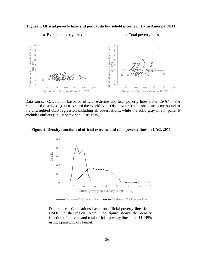
Figure 1 shows the relationship between official per capita extreme (panel a) and total (panel b)
poverty lines and per-capita household income from harmonized household surveys in the
SEDLAC database in 2011.16 The figure reports the nominal value of poverty lines – at 2011
PPP values17 – for 18 countries in Latin America at the highest possible level of geographical
14 Bourguignon (2015) presents a detailed evaluation of the SEDLAC data set.
15 NSO’s statistics and SEDLAC figures serve different purposes. The first ones are the best possible representation
of individual countries, while the second ones represent regional comparable indicators. Therefore, poverty
estimates presented in this paper should not be interpreted as a claim of methodological superiority over official
poverty estimates.
16 The existing relationship in the graph may be considered spurious if poverty lines were calculated based on the
same household surveys used in the graph. This is not the case for the countries covered in this paper; all poverty
lines have been computed in different household surveys from the ones used in the figure.
17 For those cases for which the poverty lines were not reported at 2011 PPP values, we deflated the closest value
using national CPIs. Although countries have already published lines for more recent years, we prefer to use the
figures corresponding to the nearest year as the last 2011 PPP round.
10
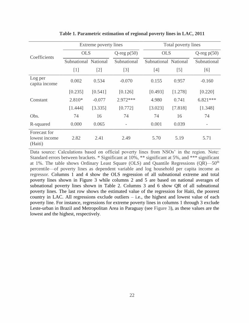
disaggregation.18 Unlike some studies for the developing world,19 Figure 1 suggests that in Latin
America there is not a significant correlation between the value of the poverty line and the level
of per capita income. This result is valid for different regression specifications (seeTable 1) using
poverty lines both at the subnational, as well as at the national (i.e., population-weighted average
of subnational lines) level. Given this result, we decided to consider all available information to
compute regional poverty lines, rather than only data from the poorest economies, as done by
Ravallion, Chen, and Sangraula (2009).
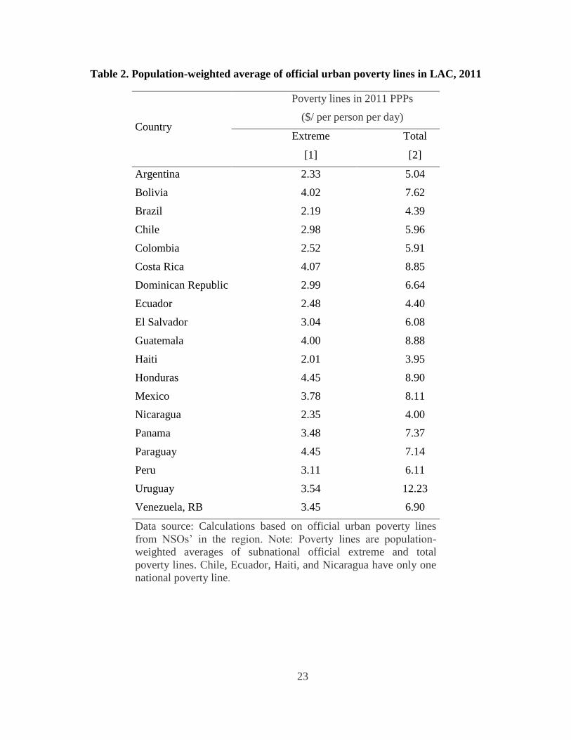
Table 2 presents population-weighted averages of extreme and total urban official
poverty lines for all countries in Latin America in 2011, and Figure 2 shows the density function
of all subnational official poverty lines. Extreme poverty lines fall within a limited range
between $2 and $4.4 per person per day, while total poverty lines are more disperse, ranging
from $4 to $12.2 per person per day. This implies that the total poverty lines of some countries
are lower in PPP terms than the extreme poverty line of other countries. For instance, the
population-weighted average extreme poverty line of Paraguay ($4.4 a day) is slightly higher
than the population-weighted average total poverty lines of Nicaragua, Ecuador, and Brazil.
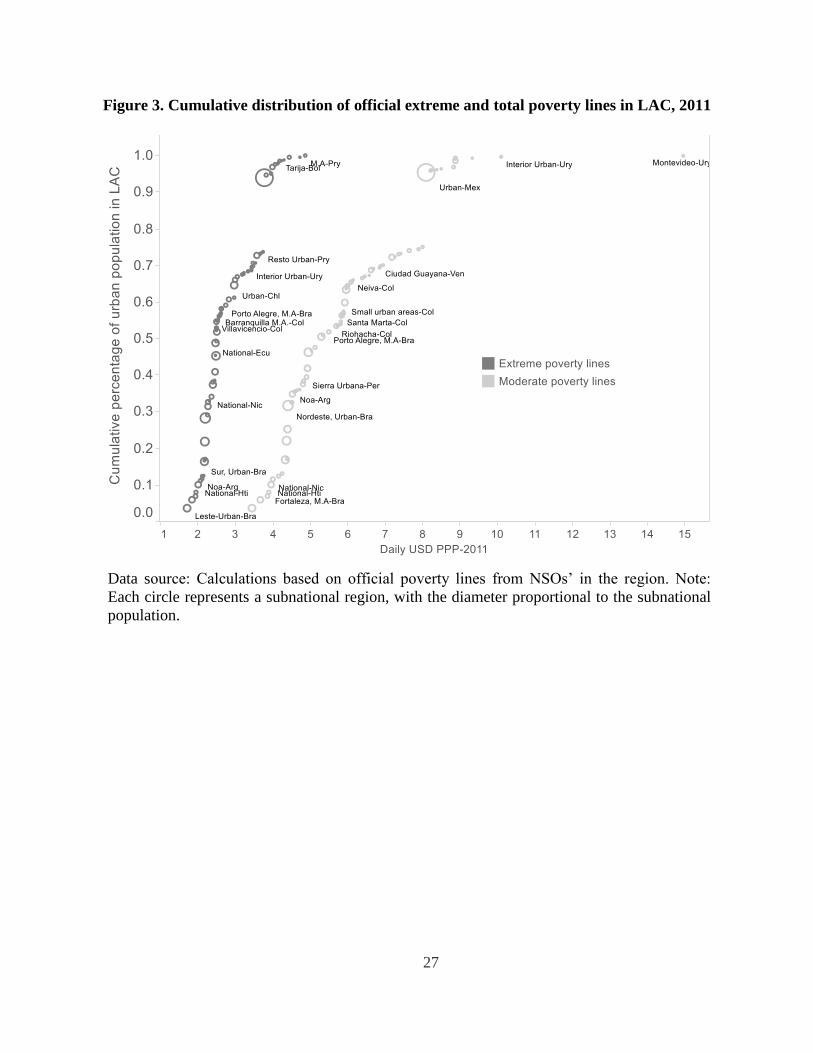
The relatively large dispersion of the total poverty lines is also evident in Figure 3, which
presents the cumulative distribution function (CDF) of the total number of official extreme and
total urban poverty lines at the subnational level. The figure shows that the rank of the
subnational regions based on the extreme official poverty lines is different from the rank based
on total official poverty lines, suggesting a large variation of the Orshansky coefficients in Latin
America. Additionally, the slope of the CDF based on extreme poverty lines is steeper than the
one based on total poverty lines, which suggest that there is more heterogeneity in the normative
cost of living when non-food items are added to the overall household consumption bundle.
Additional key messages emerge from Figure 3. First, there is a substantial overlap
between subnational poverty lines – both extreme and total – across countries in Latin America.
Taking Brazil as an example, Leste-Urban Area has the lowest total poverty line ($3.5 per person
per day) in Latin America, which is considerably lower than the total poverty line of Region
Pampeana in Argentina ($4.8 per person per day). By contrast, the metropolitan Area of Porto
Alegre in Brazil has a total poverty line of $5.5 per person per day, which is above the median
total poverty line in Latin America ($5.3 per person per day) and considerably higher than total
18 For the case of Chile, Ecuador, Haiti, and Nicaragua, the official poverty lines are published at the national level
and there is no distinction between urban and rural areas or subnational regions.
19 Ravallion et al. (2009), Ferreira et al. (2016), Jolliffe and Prydz (2016).
11
poverty lines in subnational areas of Argentina. Second, there is large heterogeneity in terms of
the number of subnational poverty lines by countries. For instance, Colombia has 23 regional
poverty lines, whereas Chile, Ecuador, Haiti, and Nicaragua have only one national poverty line.
Finally, there are some extreme values of national poverty lines that could substantially increase
the mean value of the regional poverty lines. For instance, Montevideo-Uruguay’s total poverty
line is $14.9 per person per day, which is considerably higher than the rest of the total poverty
lines in Latin America.
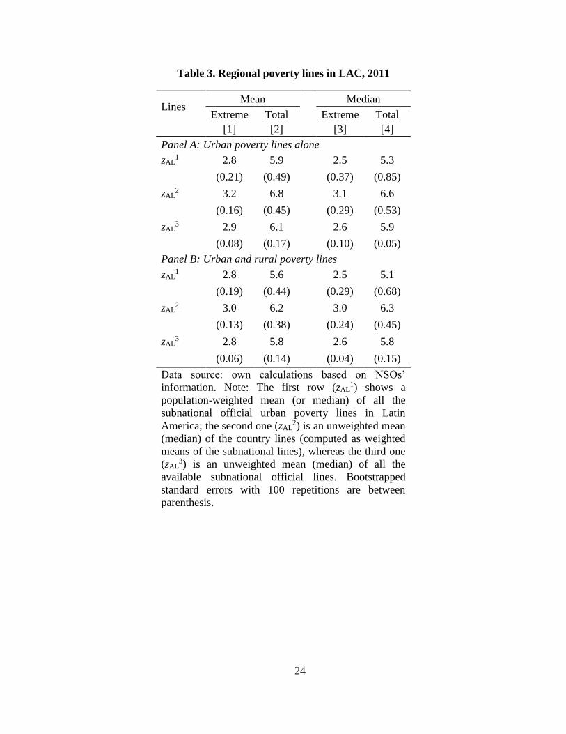
Panel A of Table 3 presents the mean and median of the extreme and total urban poverty
lines in Latin America in US dollars a day per person at PPP, using different weights according
to equations [1] to [3] above. The first row (zAL1) shows a population-weighted mean (or median)
of all the subnational official urban poverty lines in Latin America; the second row (zAL2) shows
the unweighted mean (median) of the country lines, computed as population-weighted means of
the subnational lines, whereas the third one (zAL3) is an unweighted mean (median) of all the
available subnational official lines.
Regional extreme poverty lines based on the most up-to-date official extreme poverty
lines are approximately $3 per person per day on average, while regional total poverty lines are
approximately $6 per person per day on average. However, there is variation across different
specifications in the table. Extreme and total regional poverty lines based on mean values of the
official poverty lines are higher than those based on median values, which provides evidence of
the impact that outliers have on regional averages of poverty lines. Similarly, unweighted
poverty lines are higher than the population-weighted poverty lines, which is evidence of the
existing heterogeneity in terms of the size of the subnational population and the number of
poverty lines by country.
Panel B of Table 3 test the robustness of the estimates to the inclusion of rural poverty
lines. Since the 2011 ICP round collected prices in Latin America only for urban areas, the rural
poverty lines are deflated using an urban PPP factor in panel B of the table. Results remain fairly
stable. However, the deflation of rural poverty lines using an urban PPP factor underestimates
the value of the regional poverty line if they are not adjusted by urban prices first. Therefore, we
prefer to avoid the use of rural poverty lines in our estimates.
As discussed above, although poverty lines are social constructions and poverty analysis
could be carried out without reference to a given line, in practice it has proved useful to define a
sensitive “focal” value for the poverty line that helps to simplify the discussions. In that sense,
and given the results in Table 3, we propose the use of the poverty lines of 3 and 6 US dollars per
person per day at 2011 PPP as focal regional lines for poverty comparison in Latin America.
12
Based on these two lines, we then illustrate the sensitivity of the poverty rates to the value of the
poverty lines when changing the PPP values, the period of reference, and the relative cost of
living across countries.
4 Poverty estimates
In this section, we compute poverty headcount ratios based on the regional poverty lines
suggested in Table 3. As discussed above, and given the lack of rural data for the PPP
adjustments, the regional lines are only urban. However, in this section we decided to report
national poverty estimates, since national statistics are the ones usually considered in the policy
debates. As a rough approximation to consider lower consumption prices in rural areas we follow
Deaton and Dupriez (2011) and Chen and Ravallion (2010) and multiply all rural incomes by the
ratio between urban to rural poverty lines.20
Using the set of extreme poverty lines shown in Table 3 (between $2.5 and $3.2 per
person per day), the extreme poverty rate would have ranged from 7 to 11 percent in 2013.
Similarly, using the total poverty lines (between $5.3 and $6.8 per person per day), the total
poverty rate would have varied from 24 to 35 percent in the same year.
As we showed above, the difference in the number of subnational poverty lines by
country, the presence of outliers, and the size of the subnational population affect the value of the
poverty line. For the sake of simplicity, the following analysis uses $3 and $6 per person per day
as the values for the extreme and total poverty lines, respectively. When rounded, these values
result from averaging each column of Table 3.
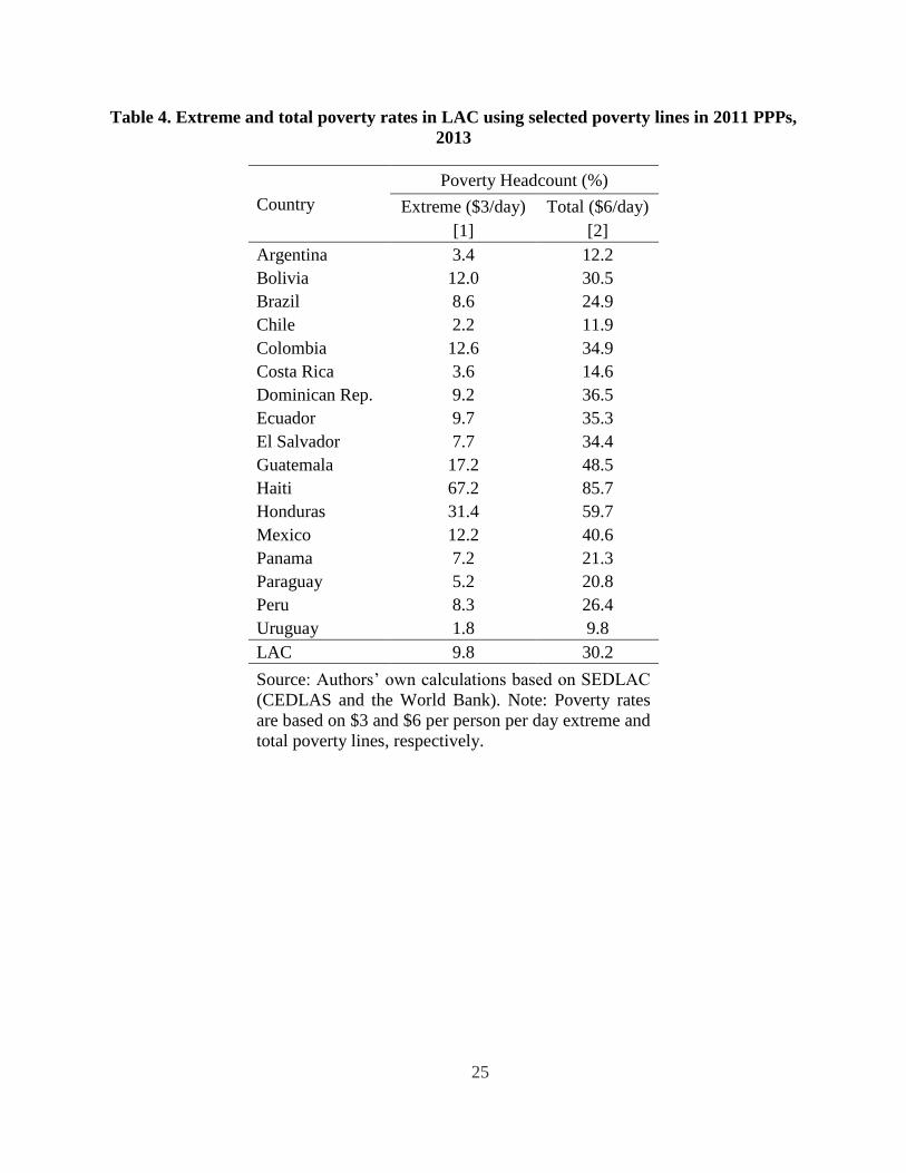
Table 4 presents the country-specific poverty estimates in 2013 based on these selected
extreme and total poverty lines and the 2011 PPPs. Poverty headcounts vary considerably across
countries in Latin America. For instance, Uruguay has the lowest extreme and total poverty rate
in Latin America, with approximately 1.8 and 9.8 percent of the population living with a per
capita income lower than $3 and $6 per person per day in 2013, respectively. On the other
extreme Haiti has the highest extreme and total poverty rate; approximately 67.2 and 85.7
percent of the population live with a per capita income lower than $3 and $6 per person per day,
respectively.
20 We use the average value of all the country specific urban to rural poverty lines ratios for countries that have only
one poverty line.
13
The last row of Table 4 shows the extreme and total poverty rates in Latin America as a
whole based on the $3 and $6 per person per day poverty lines and the 2011 PPPs. By 2013,
approximately 9.8 percent of the population lived with a per capita household income lower than
$3 per person per day in 2011 PPPs. Similarly, approximately one in three Latin Americans
qualified as poor in 2013, living with a per capita household income lower than $6 per person per
day.
5 Comparison with other lines
As commented above, and given the lack of a study on regional poverty lines, researchers and
The World Bank have been using the lines of $2.5 and $4 at 2005 PPP. It is interesting to
analyze whether the poverty rates computed with these lines substantially differ from the ones
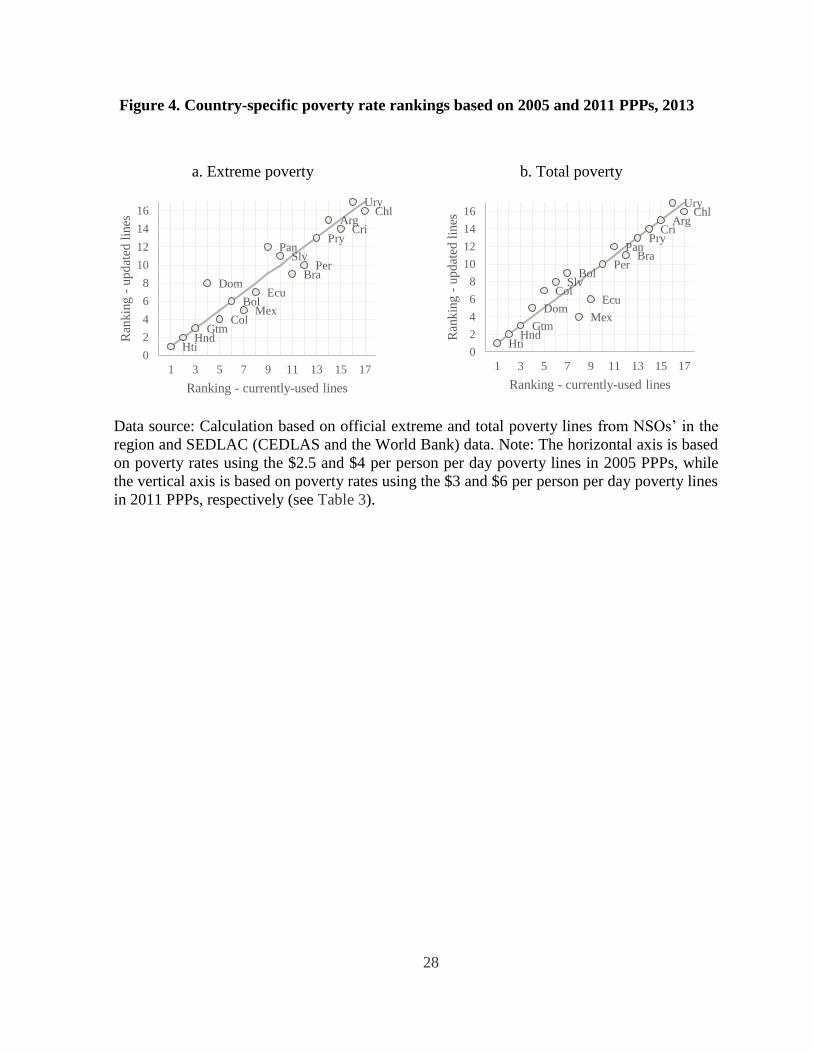
under our proposal. To explore this issue, Figure 4 presents the comparison between country-
specific extreme and total poverty rankings based on the $3 and $6 per person per day poverty
lines and the 2011 PPPs with the corresponding estimates based on the $2.5 and $4 per person
per day poverty lines and the 2005 PPPs. Any deviation from the 45-degree line denotes
differences between the poverty rankings. The figure shows that, with few exceptions, most
notably the Dominican Republican and Mexico, country-specific extreme and total poverty
rankings are generally stable to the value of the poverty lines.
Poverty headcounts calculated using 2011 PPP values differ from those calculated using
2005 PPP values, not only because the value of the poverty lines is different, but also because the
base year (i.e., 2005 or 2011) and the relative costs of living between countries (i.e., 2011 PPP
round or 2005 PPP round) are different. For instance, an extreme poverty line of $2.5 per person
per day in 2005 PPP values is different from an extreme poverty line of $2.5 per person per day
in 2011 PPP values. As explained above, the $2.5 per person per day poverty line at 2011 PPP
values is lower, in real terms, than a $2.5 per person per day poverty line at 2005 PPP values.
The difference between the headcounts calculated with both poverty lines is due not only to the
general inflation in prices that all the countries experienced, but also to the fact that (i) the
relative prices between countries – reflected in the PPP values – changed from 2005 and 2011,
and (ii) the set of underlying official poverty lines used to calculate the regional lines also
changed. In this case, to obtain the same poverty rate of the $2.5 line at 2005 PPP values in 2011
PPP values, it is necessary to set the poverty lines at $3.2 per person per day.
Thus, the difference between the poverty headcounts using both the poverty lines in 2005
PPP values and the ones in 2011 PPP values can be decomposed into three components. The first
14
component is the change of the level of the nominal value of the poverty line. In the case of the
extreme poverty line, the nominal value of the line in our example changed from $2.5 to $3 per
person per day and from $4 to $6 per person per day for the case of the total poverty line. The
second component is the effect of changing the base period from 2005 PPP values to 2011 PPP
values. That is, the welfare aggregate of each country is deflated to either 2005 or 2011 PPP
values using its corresponding CPI. As the CPI of each country evolved differently over time, the
welfare distribution of the Latin American region as a whole would differ depending on whether
the base year is 2005 or 2011. Finally, the third component is the effect of changing the spatial
deflator (i.e., relative prices) from 2005 PPP to 2011 PPP. Most of the countries in Latin
America—except for Guatemala, Panama, Peru, and El Salvador—experienced a depreciation of
their currencies as the 2011 PPP values are higher than the 2005 PPP values.
To understand the effect of each component mentioned above, we estimate the Shapley
value of the marginal effect of each component in the change of poverty headcount. That is, by
leaving two of the components constant, we change one of the components from its
corresponding value in 2005 PPP values to its value in 2011 PPP values. Then, we repeat this
process five more times until we have calculated all the possible combinations.21
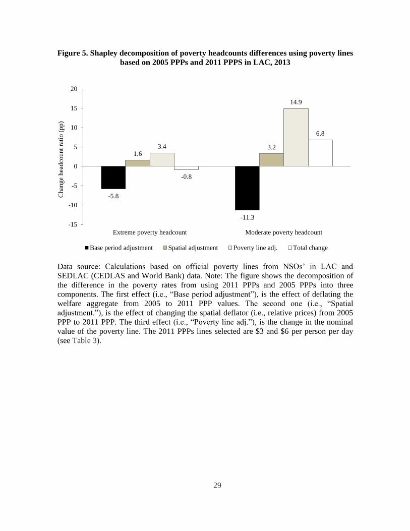
Figure 5 shows the results of the Shapley decomposition for the changes in both extreme
and total poverty using the welfare aggregate of the closest household survey of each country to
2013. In the case of total poverty, the decomposition shows a substantial poverty-increasing
effect of 14.9 percentage points from changing the nominal value of the poverty line and leaving
unchanged the other two components. However, the currently-used $4 per person per day
poverty line at 2005 PPP values and the $6 per person per day poverty line at 2011 PPP values
are expressed in different spatial and temporal units. With respect to the PPP effect (i.e., the
spatial adjustment effect), poverty headcount would increase by 3.2 percentage points,
everything else constant, and the base period effect (i.e., the temporal adjustment effect), would
reduce poverty by 11.3 percentage points, counterbalancing the significant positive effect of
changing the nominal value of the poverty line. The net change is approximately 6.8 percentage
points in 2013. On the other hand, the base period effect offsets the positive contribution of the
PPP and the nominal value effects to the extreme poverty rate, leaving the proportion of extreme
poor unchanged in 2013.
21 The number of possible combinations is equal to the factorial (n!) of the number of components. See the annex
for more technical details.
15
Unlike the majority of countries in Africa and South Asia, where the changes in poverty
measurement using the 2011 PPP values reinforced poverty reduction (Dykstra, Kenny, and
Sandefur 2014), the poverty measurement with the 2011 PPP values leads to an increase in total
poverty in Latin America and does not affect the extreme poverty.
6 Concluding remarks
Most countries monitor their own citizens’ welfare and measure their living conditions on a
regular basis. However, poverty measurement methodologies vary considerably across countries,
which makes cross-country comparison and aggregations into regional and global trends
difficult. To assess the world population’s welfare, international organizations and researchers
have promoted standardized methods to determine comparable cross-country poverty estimates
by harmonizing a spatially-deflated welfare aggregate and by estimating a unique poverty line.
At the regional level, $2.5 and $4 per person per day at 2005 PPP values have become the
poverty lines widely used in Latin America. Using these lines, 12 percent of the population in the
region qualified as extremely poor in 2013, while 24 percent qualified as poor during the same
year.
This paper provides inputs to guide the update of regional extreme and total poverty lines
for measuring poverty in Latin America as a whole, and it is the first attempt to explicitly
propose and document these inputs in the region. The recently released 2011 PPPs represent an
excellent opportunity to estimate regional extreme and total poverty lines in Latin America. To
achieve this objective, we collected the most comprehensive and up-to-date available
information on extreme and total official urban poverty lines combined with the standardized
microdata available under the SEDLAC project. Unlike previous global estimates, we do not find
a strong relationship between per capita income and the value of the poverty line. Therefore, we
did not exclude any countries from regional estimates in LAC.
This paper sets regional extreme and total poverty lines ranging from $2.5 to $3.2 and
from $5 to $6.8 per person per day, respectively. Depending on the regional poverty line
selected, we find that approximately 7 to 11 percent of Latin America’s population qualified as
extremely poor in 2013, while approximately 24 to 35 percent of the population qualified as
poor. To illustrate the sensitiveness of the poverty rate to the value of the poverty line, we
compare the results of using $3 and $6 US dollars per person per day at 2011 PPP with the $2.5
and $4 dollars per person per day at 2005 PPP. The poverty lines with the 2011 PPP values lead
to an increase in total poverty rates in Latin America with respect to the 2005 PPP values, while

16
they leave the extreme poverty rate unaffected. We believe that the approach described in this
paper, together with the results and underlying data, could serve as valuable inputs for guiding
the regional debate on poverty measurement in Latin America.
17
References
Ahluwalia, Montek S., Nicholas G. Carter, and Hollis B. Chenery. 1979. “Growth and Poverty in
Developing Countries.” Journal of Development Economics 6 (3): 299–341.
doi:10.1016/0304-3878(79)90020-8.
Bourguignon, François. 2015. Appraising income inequality databases in Latin America. Journal
of Economic Inequality, 13(4), 557–578.
CEDLAS, and World Bank. 2015. “SEDLAC: Socio-Economic Database for Latin America and
the Caribbean.” SEDLAC. August. http://sedlac.econo.unlp.edu.ar/eng/.
Chen, Shaohua, and Martin Ravallion. 2001. “How Did the World’s Poorest Fare in the 1990s?”
The Review of Income and Wealth 47 (3): 283–300. doi:10.1111/1475-4991.00018.
———. 2010. “The Developing World Is Poorer than We Thought, But No Less Successful in
the Fight Against Poverty.” The Quarterly Journal of Economics 125 (4): 1577–1625.
doi:10.1162/qjec.2010.125.4.1577.
Deaton, Angus. 1997. The analysis of household surveys: a microeconometric approach to
development policy (English). Washington, D.C.: The World Bank.
Deaton, Angus. 2010. “Price Indexes, Inequality, and the Measurement of World Poverty.” The
American Economic Review 100 (1): i-34. doi:10.1257/aer.100.1.5.
Deaton, A, and O Dupriez. 2011. “Purchasing power parity exchange rates for the global poor.”
American Economic Journal: Applied 3: 137-166.
Dykstra, Sarah, Charles Kenny, and Justin Sandefur. 2014. “Global Absolute Poverty Fell by
Almost Half on Tuesday.” Center For Global Development. May 2.
http://www.cgdev.org/blog/global-absolute-poverty-fell-almost-half-tuesday.
Ferreira, Francisco H. G., Shaohua Chen, Andrew L. Dabalen, Yuri M. Dikhanov, Nada
Hamadeh, Dean Mitchell Jolliffe, Ambar Narayan, et al. 2016. “A Global Count of the
Extreme Poor in 2012: Data Issues, Methodology and Initial Results.” The Journal of
Economic Inequality 14 (2): 141–72. doi:10.1007/s10888-016-9326-6.
Ferreira, Francisco H. G., Julian Messina, Jamele Rigolini, Luis-Felipe Lopez-Calva, Maria Ana
Lugo, and Renos Vakis. 2012. “Economic Mobility and the Rise of the Latin American
Middle Class.” 73823. The World Bank.
http://documents.worldbank.org/curated/en/2012/11/16988965/economic-mobility-rise-
latin-american-middle-class.
Gasparini, Leonardo, Martín Cicowiez, and Walter Sosa Escudero. 2013. Pobreza y desigualdad
en América Latina: conceptos, herramientas y aplicaciones. La Plata, Argentina: Temas
Grupo Editorial Srl.
IPEA. 2014. “Linhas Pobreza Regionais.” IPEA.
http://www.ipeadata.gov.br/doc/LinhasPobrezaRegionais.xls.
18
Jolliffe, Dean Mitchell, and Espen Beer Prydz. 2015. “Global Poverty Goals and Prices : How
Purchasing Power Parity Matters.” Policy Research Working Paper Series 7256. The
World Bank. https://ideas.repec.org/p/wbk/wbrwps/7256.html.
Jolliffe, Dean, and Espen Beer Prydz. 2016. “Estimating International Poverty Lines from
Comparable National Thresholds.” The Journal of Economic Inequality 14 (2): 185–98.
doi:10.1007/s10888-016-9327-5.
López-Calva, Luis F., and Eduardo Ortiz-Juarez. 2014. “A Vulnerability Approach to the
Definition of the Middle Class.” The Journal of Economic Inequality 12 (1): 23–47.
doi:10.1007/s10888-012-9240-5.
Orshansky, M. (1963). "Children of the poor". Social Security Bulletin 26.
Ravallion, Martin. 2018. "An Exploration of the International Comparison Program's New
Global Economic Landscape," World Development. 105: 201-216.
Ravallion, Martin, Shaohua Chen, and Prem Sangraula. 2009. “Dollar a Day Revisited.” The
World Bank Economic Review, June, lhp007. doi:10.1093/wber/lhp007.
Ravallion, Martin, Gaurav Datt, and Dominique van de Walle. 1991. “Quantifying Absolute
Poverty in the Developing World.” Review of Income and Wealth 37 (4): 345–61.
doi:10.1111/j.1475-4991.1991.tb00378.x.
Stampini, Marco, Marcos Robles, Mayra Sáenz, Pablo Ibarrarán, and Nadin Medellín. 2016.
"Poverty, vulnerability, and the middle class in Latin America." Latin American
Economic Review
Shorrocks, Anthony F. 2012. “Decomposition Procedures for Distributional Analysis: A Unified
Framework Based on the Shapley Value.” The Journal of Economic Inequality 11 (1):
99–126. doi:10.1007/s10888-011-9214-z.
World Bank. 2011. “On the Edge of Uncertainty : Poverty Reduction in Latin America and the
Caribbean during the Great Recession and Beyond.”
https://openknowledge.worldbank.org/handle/10986/17196.
———. 2013. “Shifting Gears to Accelerate Shared Prosperity in Latin America and
Caribbean.” 78507. The World Bank.
http://documents.worldbank.org/curated/en/2013/06/17872255/shifting-gears-accelerate-
shared-prosperity-latin-america-caribbean.
———. 2014b. “Social Gains in the Balance : A Fiscal Policy Challenge for Latin America and
the Caribbean.” 85162. The World Bank.
http://documents.worldbank.org/curated/en/2014/02/19567116/social-gains-balance-
fiscal-policy-challenge-latin-america-caribbean.
———. 2015. “Working to End Poverty in Latin America and the Caribbean: Workers, Jobs,
and Wages.” Washington, DC.: The World Bank. http://hdl.handle.net/10986/22016.
19
Annex A. Shapley decomposition of change in regional poverty methodology from PPP
2005 to PPP 2011
A poverty rate 𝑃𝑠 could be defined as non-linear function 𝜑 with components 𝑠—poverty line,
CPI, and PPP. There are two possible values for: {𝑎, 𝑟} , where 𝑎 and 𝑟 refer to the proper set of
components used to estimate the poverty headcount using either alternative (a) or currently-used
(r) poverty lines. Thus, the poverty rate is defined as 𝑃𝑠 = 𝜑(𝑦𝑠, 𝑧𝑠); where 𝑧𝑠 represents the
poverty line of the set of components 𝑠, while 𝑦𝑠𝑡 = 𝜋(𝑦, 𝑐𝑝𝑖𝑠, 𝑝𝑝𝑝𝑠) is a vector of household
incomes in time t that has been deflated using the set of components 𝑠.
Under this framework, equation (1) shows that the difference between 𝑃𝑎 and 𝑃𝑟 is not
wholly due to changes in the poverty line, but also to spatial and temporal deflation using PPP
and CPI, respectively.
𝑃𝑎 − 𝑃𝑟 = 𝜑(𝑦𝑎, 𝑧𝑎) − 𝜑(𝑦𝑟 , 𝑧𝑟)
(1)
Given that the differences between the two welfare distributions 𝑦𝑎 and 𝑦𝑟 are fully
characterized by the use of different country specific CPI and PPP, equation (1) could be
expressed as:
𝑃𝑎 − 𝑃𝑟 = 𝜑( 𝜋(𝑦, 𝑐𝑝𝑖𝑎, 𝑝𝑝𝑝𝑎), 𝑧𝑎) − 𝜑(𝜋(𝑦, 𝑐𝑝𝑖𝑟 , 𝑝𝑝𝑝𝑟), 𝑧𝑟) (2)
Notice that the poverty headcount function 𝜑 is not additively separable among its
components, which means that the sum of the marginal effects of all the components is not equal
to the total change. Therefore, in order to understand the contribution of each of the components,
a decomposition procedure for distributional analysis based on the Shapley value suggested by
Shorrocks (2012) is applied to estimate the relative weight of each component of the difference
in equation (2).
The Shapley-Shorrocks procedure consists of constructing a counterfactual headcount
based on different combinations of components by substituting each component at a time. Then,
the poverty headcount obtained by modifying only one component at a time, say the PPP
component (𝜑( 𝜋(𝑦, 𝑐𝑝𝑖𝑎, 𝑝𝑝𝑝𝑏), 𝑧𝑎)), would play the role of a counterfactual headcount of the
PPP component, which can be interpreted as the poverty headcount obtained if the PPP had
changed while the other components remained constant. Thus, the marginal contribution of the
PPP would be the differences between the counterfactual headcount and the observed headcount,
𝜑( 𝜋(𝑦, 𝑐𝑝𝑖𝑎, 𝑝𝑝𝑝𝑎), 𝑧𝑎). As explained above, given that the poverty headcount is a function of
20
three components, the procedure above is done six times to account for all possible
combinations.22
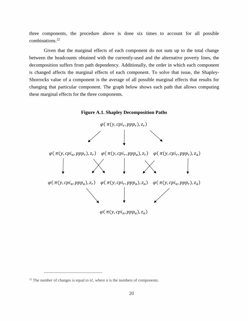
Given that the marginal effects of each component do not sum up to the total change
between the headcounts obtained with the currently-used and the alternative poverty lines, the
decomposition suffers from path dependency. Additionally, the order in which each component
is changed affects the marginal effects of each component. To solve that issue, the Shapley-
Shorrocks value of a component is the average of all possible marginal effects that results for
changing that particular component. The graph below shows each path that allows computing
these marginal effects for the three components.
Figure A.1. Shapley Decomposition Paths
𝜑( 𝜋(𝑦, 𝑐𝑝𝑖𝑟 , 𝑝𝑝𝑝𝑟), 𝑧𝑟)
𝜑( 𝜋(𝑦, 𝑐𝑝𝑖𝑎, 𝑝𝑝𝑝𝑟), 𝑧𝑟) 𝜑( 𝜋(𝑦, 𝑐𝑝𝑖𝑟 , 𝑝𝑝𝑝𝑎), 𝑧𝑟) 𝜑( 𝜋(𝑦, 𝑐𝑝𝑖𝑟 , 𝑝𝑝𝑝𝑟), 𝑧𝑎)
𝜑( 𝜋(𝑦, 𝑐𝑝𝑖𝑎, 𝑝𝑝𝑝𝑎), 𝑧𝑟) 𝜑( 𝜋(𝑦, 𝑐𝑝𝑖𝑟 , 𝑝𝑝𝑝𝑎), 𝑧𝑎) 𝜑( 𝜋(𝑦, 𝑐𝑝𝑖𝑎, 𝑝𝑝𝑝𝑟), 𝑧𝑎)
𝜑( 𝜋(𝑦, 𝑐𝑝𝑖𝑎, 𝑝𝑝𝑝𝑎), 𝑧𝑎)
22 The number of changes is equal to n!, where n is the numbers of components.
21
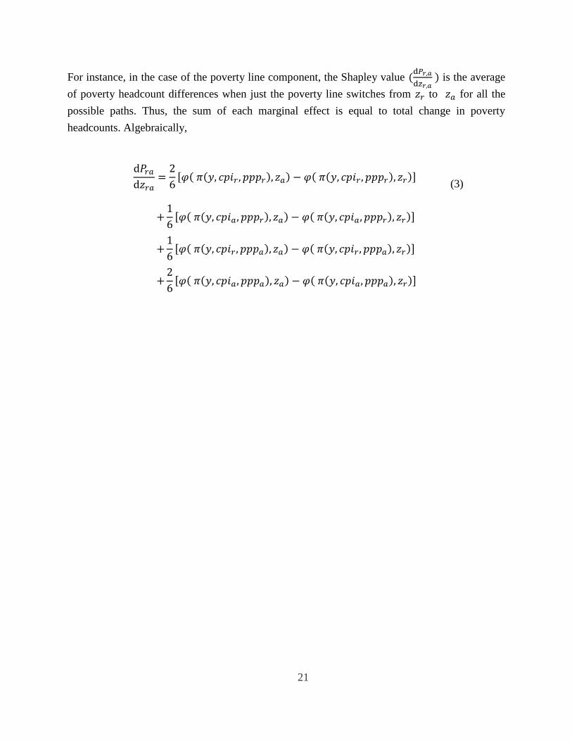
For instance, in the case of the poverty line component, the Shapley value (d𝑃𝑟,𝑎
d𝑧𝑟,𝑎 ) is the average
of poverty headcount differences when just the poverty line switches from 𝑧𝑟 to 𝑧𝑎 for all the
possible paths. Thus, the sum of each marginal effect is equal to total change in poverty
headcounts. Algebraically,
d𝑃𝑟𝑎
d𝑧𝑟𝑎=
2
6[𝜑( 𝜋(𝑦, 𝑐𝑝𝑖𝑟 , 𝑝𝑝𝑝𝑟), 𝑧𝑎) − 𝜑( 𝜋(𝑦, 𝑐𝑝𝑖𝑟 , 𝑝𝑝𝑝𝑟), 𝑧𝑟)]
(3)
+1
6[𝜑( 𝜋(𝑦, 𝑐𝑝𝑖𝑎, 𝑝𝑝𝑝𝑟), 𝑧𝑎) − 𝜑( 𝜋(𝑦, 𝑐𝑝𝑖𝑎, 𝑝𝑝𝑝𝑟), 𝑧𝑟)]
+1
6[𝜑( 𝜋(𝑦, 𝑐𝑝𝑖𝑟 , 𝑝𝑝𝑝𝑎), 𝑧𝑎) − 𝜑( 𝜋(𝑦, 𝑐𝑝𝑖𝑟 , 𝑝𝑝𝑝𝑎), 𝑧𝑟)]
+2
6[𝜑( 𝜋(𝑦, 𝑐𝑝𝑖𝑎, 𝑝𝑝𝑝𝑎), 𝑧𝑎) − 𝜑( 𝜋(𝑦, 𝑐𝑝𝑖𝑎, 𝑝𝑝𝑝𝑎), 𝑧𝑟)]
22
Table 1. Parametric estimation of regional poverty lines in LAC, 2011
Coefficients
Extreme poverty lines
Total poverty lines
OLS
Q-reg p(50)
OLS
Q-reg p(50)
Subnational National
Subnational
Subnational National
Subnational
[1] [2]
[3]
[4] [5]
[6]
Log per
capita income 0.002 0.534
-0.070
0.155 0.957
-0.160
[0.235] [0.541]
[0.126]
[0.493] [1.278]
[0.220]
Constant 2.810* -0.077
2.972***
4.980 0.741
6.821***
[1.444] [3.335]
[0.772]
[3.023] [7.818]
[1.348]
Obs. 74 16
74
74 16
74
R-squared 0.000 0.065
-
0.001 0.039
-
Forecast for
lowest income
(Haiti)
2.82 2.41
2.49
5.70 5.19
5.71
Data source: Calculations based on official poverty lines from NSOs’ in the region. Note:
Standard errors between brackets. * Significant at 10%, ** significant at 5%, and *** significant
at 1%. The table shows Ordinary Least Square (OLS) and Quantile Regressions (QR)—50th
percentile—of poverty lines as dependent variable and log household per capita income as
regressor. Columns 1 and 4 show the OLS regression of all subnational extreme and total
poverty lines shown in Figure 3 while columns 2 and 5 are based on national averages of
subnational poverty lines shown in Table 2. Columns 3 and 6 show QR of all subnational
poverty lines. The last row shows the estimated value of the regression for Haiti, the poorest
country in LAC. All regressions exclude outliers – i.e., the highest and lowest value of each
poverty line. For instance, regressions for extreme poverty lines in columns 1 through 3 exclude
Leste-urban in Brazil and Metropolitan Area in Paraguay (see Figure 3), as these values are the
lowest and the highest, respectively.
23
Table 2. Population-weighted average of official urban poverty lines in LAC, 2011
Country
Poverty lines in 2011 PPPs
($/ per person per day)
Extreme Total
[1] [2]
Argentina 2.33 5.04
Bolivia 4.02 7.62
Brazil 2.19 4.39
Chile 2.98 5.96
Colombia 2.52 5.91
Costa Rica 4.07 8.85
Dominican Republic 2.99 6.64
Ecuador 2.48 4.40
El Salvador 3.04 6.08
Guatemala 4.00 8.88
Haiti 2.01 3.95
Honduras 4.45 8.90
Mexico 3.78 8.11
Nicaragua 2.35 4.00
Panama 3.48 7.37
Paraguay 4.45 7.14
Peru 3.11 6.11
Uruguay 3.54 12.23
Venezuela, RB 3.45 6.90
Data source: Calculations based on official urban poverty lines
from NSOs’ in the region. Note: Poverty lines are population-
weighted averages of subnational official extreme and total
poverty lines. Chile, Ecuador, Haiti, and Nicaragua have only one
national poverty line.
24
Table 3. Regional poverty lines in LAC, 2011
Lines Mean Median
Extreme Total Extreme Total
[1] [2] [3] [4]
Panel A: Urban poverty lines alone
zAL1 2.8 5.9 2.5 5.3
(0.21) (0.49) (0.37) (0.85)
zAL2 3.2 6.8 3.1 6.6
(0.16) (0.45) (0.29) (0.53)
zAL3 2.9 6.1 2.6 5.9
(0.08) (0.17) (0.10) (0.05)
Panel B: Urban and rural poverty lines
zAL1 2.8 5.6 2.5 5.1
(0.19) (0.44) (0.29) (0.68)
zAL2 3.0 6.2 3.0 6.3
(0.13) (0.38) (0.24) (0.45)
zAL3 2.8 5.8 2.6 5.8
(0.06) (0.14) (0.04) (0.15)
Data source: own calculations based on NSOs’
information. Note: The first row (zAL1) shows a
population-weighted mean (or median) of all the
subnational official urban poverty lines in Latin
America; the second one (zAL2) is an unweighted mean
(median) of the country lines (computed as weighted
means of the subnational lines), whereas the third one
(zAL3) is an unweighted mean (median) of all the
available subnational official lines. Bootstrapped
standard errors with 100 repetitions are between
parenthesis.
25
Table 4. Extreme and total poverty rates in LAC using selected poverty lines in 2011 PPPs,
2013
Country
Poverty Headcount (%)
Extreme ($3/day) Total ($6/day)
[1] [2]
Argentina 3.4 12.2
Bolivia 12.0 30.5
Brazil 8.6 24.9
Chile 2.2 11.9
Colombia 12.6 34.9
Costa Rica 3.6 14.6
Dominican Rep. 9.2 36.5
Ecuador 9.7 35.3
El Salvador 7.7 34.4
Guatemala 17.2 48.5
Haiti 67.2 85.7
Honduras 31.4 59.7
Mexico 12.2 40.6
Panama 7.2 21.3
Paraguay 5.2 20.8
Peru 8.3 26.4
Uruguay 1.8 9.8
LAC 9.8 30.2
Source: Authors’ own calculations based on SEDLAC
(CEDLAS and the World Bank). Note: Poverty rates
are based on $3 and $6 per person per day extreme and
total poverty lines, respectively.
26
Figure 1. Official poverty lines and per capita household income in Latin America, 2011
a. Extreme poverty lines b. Total poverty lines
Data source: Calculation based on official extreme and total poverty lines from NSOs’ in the
region and SEDLAC (CEDLAS and the World Bank) data. Note: The dashed lines correspond to
the unweighted OLS regression including all observations, while the solid gray line in panel b
excludes outliers (i.e., Montevideo – Uruguay).
Figure 2. Density functions of official extreme and total poverty lines in LAC, 2011
Data source: Calculations based on official poverty lines from
NSOs’ in the region. Note: The figure shows the density
function of extreme and total official poverty lines in 2011 PPPs
using Epanechnikov kernel.
0
2
4
6
8
10
12
14
16
0 200 400 600 800 1,000 1,200
Subnat
ional
extr
eme
pover
ty l
ines
($/d
ay i
n
2011 P
PP
)
Per capita household income ($/month 2011 PPP)
0
2
4
6
8
10
12
14
16
0 200 400 600 800 1,000 1,200Subnat
ional
moder
ate
pover
ty l
ines
($/d
ay i
n
2011 P
PP
)
Per capita household income ($/month 2011 PPP)
0
0.1
0.2
0.3
0.4
0.5
0 2 4 6 8 10 12 14 16
Den
sity
Official poverty lines ($/day in 2011 PPPs)
Extreme official poverty lines Moderate official poverty lines
27
Figure 3. Cumulative distribution of official extreme and total poverty lines in LAC, 2011
Data source: Calculations based on official poverty lines from NSOs’ in the region. Note:
Each circle represents a subnational region, with the diameter proportional to the subnational
population.
28
Figure 4. Country-specific poverty rate rankings based on 2005 and 2011 PPPs, 2013
a. Extreme poverty b. Total poverty
Data source: Calculation based on official extreme and total poverty lines from NSOs’ in the
region and SEDLAC (CEDLAS and the World Bank) data. Note: The horizontal axis is based
on poverty rates using the $2.5 and $4 per person per day poverty lines in 2005 PPPs, while
the vertical axis is based on poverty rates using the $3 and $6 per person per day poverty lines
in 2011 PPPs, respectively (see Table 3).
Arg
Bol
Bra
Chl
Col
Cri
DomEcu
Slv
Gtm
HtiHnd
Mex
PanPry
Per
Ury
0
2
4
6
8
10
12
14
16
1 3 5 7 9 11 13 15 17
Ran
kin
g -
up
dat
ed l
ines
Ranking - currently-used lines
Arg
Bol
Bra
Chl
Col
Cri
DomEcu
Slv
Gtm
HtiHnd
Mex
PanPry
Per
Ury
0
2
4
6
8
10
12
14
16
1 3 5 7 9 11 13 15 17
Ran
kin
g -
up
dat
ed l
ines
Ranking - currently-used lines
29
Figure 5. Shapley decomposition of poverty headcounts differences using poverty lines
based on 2005 PPPs and 2011 PPPS in LAC, 2013
Data source: Calculations based on official poverty lines from NSOs’ in LAC and
SEDLAC (CEDLAS and World Bank) data. Note: The figure shows the decomposition of
the difference in the poverty rates from using 2011 PPPs and 2005 PPPs into three
components. The first effect (i.e., “Base period adjustment”), is the effect of deflating the
welfare aggregate from 2005 to 2011 PPP values. The second one (i.e., “Spatial
adjustment.”), is the effect of changing the spatial deflator (i.e., relative prices) from 2005
PPP to 2011 PPP. The third effect (i.e., “Poverty line adj.”), is the change in the nominal
value of the poverty line. The 2011 PPPs lines selected are $3 and $6 per person per day
(see Table 3).
-5.8
-11.3
1.63.23.4
14.9
-0.8
6.8
-15
-10
-5
0
5
10
15
20
Extreme poverty headcount Moderate poverty headcount
Chan
ge
hea
dco
unt
rati
o (
pp
)
Base period adjustment Spatial adjustment Poverty line adj. Total change