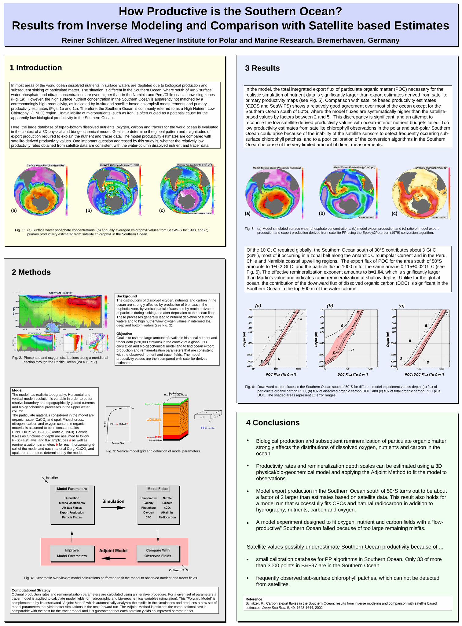
How Productive is the Southern Ocean? Results from Inverse Modeling and Comparison with Satellite based Estimates

Reiner Schlitzer, Alfred Wegener Institute for Polar and Marine Research, Bremerhaven, Germany

How Productive is the Southern Ocean? How Productive is the Southern Ocean? Results from Inverse Results from Inverse ModelingModeling and Comparison with Satellite based Estimatesand Comparison with Satellite based Estimates

Reiner Schlitzer, Alfred Wegener Institute Reiner Schlitzer, Alfred Wegener Institute forfor Polar and Marine Research, Bremerhaven, GermanyPolar and Marine Research, Bremerhaven, Germany

2 2 MethodsMethods

3 3 ResultsResults

4 4 ConclusionsConclusions

(a) Surface water phosphate concentrations, (b) annually averaged chlorophyll values from SeaWiFS for 1998, and (c) primary productivity estimated from satellite chlorophyll in the Southern Ocean.

Fig. 1:

(a) (b) (c)

1 1 IntroductionIntroduction

BackgroundThe distributions of dissolved oxygen, nutrients and carbon in the ocean are strongly affected by production of biomass in the euphotic zone, by vertical particle fluxes and by remineralization of particles during sinking and after deposition at the ocean floor. These processes generally lead to nutrient depletion of surface waters and to high nutrient/low oxygen values in intermediate, deep and bottom waters (see Fig. 2).

ObjectiveGoal is to use the large amount of available historical nutrient and tracer data (>20,000 stations) in the context of a global, 3D circulation and bio-geochemical model and to find ocean export production and remineralization parameters that are consistent with the observed nutrient and tracer fields. The model productivity values are then compared with satellite-derived estimates.

Fig. 2: Phosphate and oxygen distributions along a meridional section through the Pacific Ocean (WOCE P17).

ModelThe model has realistic topography. Horizontal and vertical model resolution is variable in order to better resolve boundary and topographically guided currents and bio-geochemical processes in the upper water column. The particulate materials considered in the model are organic tissue, CaCO3 and opal. Phosphorous, nitrogen, carbon and oxygen content in organic material is assumed to be in constant ratios P:N:C:O=1:16:106:-138 (Redfield, 1963). Particle fluxes as functions of depth are assumed to follow PF(z)=a·zb laws, and flux amplitudes a as well as remineralization parameters b for each horizontal grid-cell of the model and each material Corg, CaCO3 and opal are parameters determined by the model. Fig. 3: Vertical model grid and definition of model parameters.

Fig. 4: Schematic overview of model calculations performed to fit the model to observed nutrient and tracer fields

Computational StrategyOptimal production rates and remineralization parameters are calculated using an iterative procedure. For a given set of parameters a tracer model is applied to calculate model fields for hydrographic and bio-geochemical variables (simulation). This "Forward Model" is complemented by its associated "Adjoint Model" which automatically analyzes the misfits in the simulations and produces a new set of model parameters that yield better simulations in the next forward run. The Adjoint Method is efficient: the computational cost is comparable with the cost for the tracer model and it is guaranteed that each iteration yields an improved parameter set.

In most areas of the world ocean dissolved nutrients in surface waters are depleted due to biological production and subsequent sinking of particulate matter. The situation is different in the Southern Ocean, where south of 40°S surface water phosphate and nitrate concentrations are even higher than in the Namibia and Peru/Chile coastal upwelling zones (Fig. 1a). However, the high surface nutrient concentration in the Southern Ocean is apparently not matched by a correspondingly high productivity, as indicated by in-situ and satellite based chlorophyll measurements and primary productivity estimates (Figs. 1b and 1c). Therefore, the Southern Ocean is commonly referred to as a High Nutrient Low Chlorophyll (HNLC) region. Unavailability of micronutrients, such as iron, is often quoted as a potential cause for the apparently low biological productivity in the Southern Ocean.

Here, the large database of top-to-bottom dissolved nutrients, oxygen, carbon and tracers for the world ocean is evaluated in the context of a 3D physical and bio-geochemical model. Goal is to determine the global pattern and magnitudes of export production required to explain the nutrient and tracer data. The model productivity estimates are compared with satellite-derived productivity values. One important question addressed by this study is, whether the relatively low productivity rates obtained from satellite data are consistent with the water-column dissolved nutrient and tracer data.

Fig. 5: (a) Model simulated surface water phosphate concentrations, (b) model export production and (c) ratio of model export production and export production derived from satellite PP using the Eppley&Peterson (1979) conversion algorithm.

(a) (b) (c)

Reference:Schlitzer, R., Carbon export fluxes in the Southern Ocean: results from inverse modeling and comparison with satellite based estimates, Deep Sea Res. II, 49, 1623-1644, 2002.

In the model, the total integrated export flux of particulate organic matter (POC) necessary for the realistic simulation of nutrient data is significantly larger than export estimates derived from satellite primary productivity maps (see Fig. 5). Comparison with satellite based productivity estimates (CZCS and SeaWiFS) shows a relatively good agreement over most of the ocean except for the Southern Ocean south of 50°S, where the model fluxes are systematically higher than the satellite-based values by factors between 2 and 5. This discrepancy is significant, and an attempt to reconcile the low satellite-derived productivity values with ocean-interior nutrient budgets failed. Too low productivity estimates from satellite chlorophyll observations in the polar and sub-polar Southern Ocean could arise because of the inability of the satellite sensors to detect frequently occurring sub-surface chlorophyll patches, and to a poor calibration of the conversion algorithms in the Southern Ocean because of the very limited amount of direct measurements.

Of the 10 Gt C required globally, the Southern Ocean south of 30°S contributes about 3 Gt C (33%), most of it occurring in a zonal belt along the Antarctic Circumpolar Current and in the Peru, Chile and Namibia coastal upwelling regions. The export flux of POC for the area south of 50°S amounts to 1±0.2 Gt C, and the particle flux in 1000 m for the same area is 0.115±0.02 Gt C (see Fig. 6). The effective remineralization exponent amounts to b=1.04, which is significantly larger than Martin’s value and indicates rapid remineralization at shallow depths. Unlike for the global ocean, the contribution of the downward flux of dissolved organic carbon (DOC) is significant in the Southern Ocean in the top 500 m of the water column.

Fig. 6: Downward carbon fluxes in the Southern Ocean south of 50°S for different model experiment versus depth: (a) flux of particulate organic carbon POC, (b) flux of dissolved organic carbon DOC, and (c) flux of total organic carbon POC plus DOC. The shaded areas represent 1σ error ranges.

Biological production and subsequent remineralization of particulate organic matter strongly affects the distributions of dissolved oxygen, nutrients and carbon in the ocean.

Productivity rates and remineralization depth scales can be estimated using a 3D physical/bio-geochemical model and applying the Adjoint Method to fit the model to observations.

Model export production in the Southern Ocean south of 50°S turns out to be about a factor of 2 larger than estimates based on satellite data. This result also holds for a model run that successfully fits CFCs and natural radiocarbon in addition to hydrography, nutrients, carbon and oxygen.

A model experiment designed to fit oxygen, nutrient and carbon fields with a “low-productive” Southern Ocean failed because of too large remaining misfits.

•

•

•

•

Satellite values possibly underestimate Southern Ocean productivity because of ...

small calibration database for PP algorithms in Southern Ocean. Only 33 of more than 3000 points in B&F97 are in the Southern Ocean.

frequently observed sub-surface chlorophyll patches, which can not be detected from satellites.

•

•