How Noisy Adaptation of Neurons Shapes Interspike Interval

How Noisy Adaptation of Neurons Shapes InterspikeInterval Histograms and CorrelationsTilo Schwalger1*, Karin Fisch2, Jan Benda2, Benjamin Lindner1

1 Max-Planck Institute for the Physics of Complex Systems, Dresden, Germany, 2 Division of Neurobiology, Department Biology II, Ludwig-Maximilians-Universitat

Munchen, Munich, Germany

Abstract

Channel noise is the dominant intrinsic noise source of neurons causing variability in the timing of action potentials andinterspike intervals (ISI). Slow adaptation currents are observed in many cells and strongly shape response properties ofneurons. These currents are mediated by finite populations of ionic channels and may thus carry a substantial noisecomponent. Here we study the effect of such adaptation noise on the ISI statistics of an integrate-and-fire model neuron bymeans of analytical techniques and extensive numerical simulations. We contrast this stochastic adaptation with thecommonly studied case of a fast fluctuating current noise and a deterministic adaptation current (corresponding to aninfinite population of adaptation channels). We derive analytical approximations for the ISI density and ISI serial correlationcoefficient for both cases. For fast fluctuations and deterministic adaptation, the ISI density is well approximated by aninverse Gaussian (IG) and the ISI correlations are negative. In marked contrast, for stochastic adaptation, the density is morepeaked and has a heavier tail than an IG density and the serial correlations are positive. A numerical study of the mixed casewhere both fast fluctuations and adaptation channel noise are present reveals a smooth transition between the analyticallytractable limiting cases. Our conclusions are furthermore supported by numerical simulations of a biophysically morerealistic Hodgkin-Huxley type model. Our results could be used to infer the dominant source of noise in neurons from theirISI statistics.

Citation: Schwalger T, Fisch K, Benda J, Lindner B (2010) How Noisy Adaptation of Neurons Shapes Interspike Interval Histograms and Correlations. PLoS ComputBiol 6(12): e1001026. doi:10.1371/journal.pcbi.1001026

Editor: Peter E. Latham, Gatsby Computational Neuroscience Unit, University College London, United Kingdom

Received April 7, 2010; Accepted November 8, 2010; Published December 16, 2010

Copyright: � 2010 Schwalger et al. This is an open-access article distributed under the terms of the Creative Commons Attribution License, which permitsunrestricted use, distribution, and reproduction in any medium, provided the original author and source are credited.

Funding: KF was funded by BMBF Bernstein Collaboration for Computational Neuroscience 01GQ0722. JB was funded by BMBF Bernstein Award ComputationalNeuroscience 01GQ0802. The funders had no role in study design, data collection and analysis, decision to publish, or preparation of the manuscript.

Competing Interests: The authors have declared that no competing interests exist.

* E-mail: [email protected]

Introduction

The firing of action potentials of a neuron in vivo is a genuine

stochastic process due to the presence of several sources of noise

[1]. The spontaneous neural activity (e.g. the firing of a sensory

cell in absence of sensory stimuli) [2,3] as well as the response of

neurons to stimuli cannot be understood without taking into

account these fluctuations [4]. Moreover, noise can have a positive

influence on neural function, e.g. by stochastic resonance [5,6],

gain modulation [7], decorrelation of spiking activity [8],

enhancement of signal detection [9], or fast transmission of noise

coded signals [10,11]. For these reasons, reduced stochastic models

of neural activity have been suggested [12–14] and analytical

methods have been developed to calculate the statistics of

spontaneous activity and the response to periodic stimuli [15–

17]. Studying such reduced models allows to relate specific

mechanisms with certain statistics of neural firing. Vice versa,

analytical expressions for the firing statistics of model neurons may

be used to infer unknown physiological details from experimental

data.

Spike-frequency adaptation is another common feature of

neural dynamics that, however, is still poorly understood in the

context of stochastic spike generation. Associated adaptation

currents which act on time scales ranging from 50ms to seconds

are ubiquitous throughout the nervous system [18]. Prominent

examples of adaptation mechanisms include M-type currents,

calcium-gated potassium currents (IAHP), and slow inactivation of

sodium currents. Functional roles of spike-frequency adaptation

include forward masking [19], high-pass filtering [20–22], and

response selectivity [23–25]. If the neuron is driven by fast

fluctuations, adaptation reveals itself in the interspike interval

statistics of neural firing, most prominently in the occurrence of

negative correlations among interspike intervals [26–31]. These

features can be phenomenologically captured in generalized

integrate-and-fire (IF) models via introduction of a slow inhibitory

feedback variable, either acting as a dynamic threshold or as an

inhibitory conductance or current [28,29,32–34] or in even more

simplified models [35–37].

In previous studies on stochastic models with adaptation,

fluctuations were considered to be fast, e.g. Poissonian synaptic

spike trains passing through fast synapses or a white Gaussian

input current representing a mixture of intrinsic fluctuations and

background synaptic input. In particular, the dominating intrinsic

source of fluctuations is ion channel noise [1,38–40]. This kind of

noise is not only contributed by the fast ionic conductances, which

establish the spike generating mechanism, but also by the channels

that mediate adaptation currents. If the number of adaptation

channels is not too large, the stochastic opening and closing of

single channels will contribute a fluctuating component to the

adaptation current. This noise contribution, which was so far

PLoS Computational Biology | www.ploscompbiol.org 1 December 2010 | Volume 6 | Issue 12 | e1001026

ignored in the literature, and its impact on the ISI statistics is the

subject of our study. Here, we only consider the simplest

adaptation channel model which corresponds to an M-type

adaptation current. Our results, however, also apply to other

sources of noise emerging from a slow adaptation mechanisms as,

for instance, slow Ca2z fluctuations in the case of calcium-gated

potassium currents (see discussion).

In this paper, we analyze a perfect integrate-and-fire (PIF) model

in which a population of Na channels mediate a stochastic

adaptation current. We approximate this model by simplified

stochastic differential equations (diffusion approximation). For slow

adaptation, we are able to show that the latter is equivalent to a PIF

neuron driven by a slow external noise. As a surprising consequence,

pure adaptation channel noise induces positive ISI correlations in

marked contrast to negative ISI correlations evoked by the

commonly studied combination of fast noise and deterministic

adaptation [28]. Furthermore, the ISI histogram is more peaked and

displays a heavier tail than expected for a PIF model with fast current

noise. Our results for the PIF (positive ISI correlations, peaked

histograms) are qualitatively confirmed by extensive simulations of a

conductance-based model with Na stochastic adaptation channels

supporting the generality of our findings.

Results

Our main concern in this paper was the effect of noise

associated with the slow dynamics of adaptation on the interspike

interval statistics. Specifically, the noise was regarded as the result

of the stochastic activity of a finite number of slow ‘‘adaptation

channels’’, e.g. M-type channels ([41,42]). We contrasted this slow

adaptation channel-noise with the opposite and commonly

considered case of a deterministic adaptation mechanism together

with fast current fluctuations [28,29]. In both cases, the spike

frequency and the variability of the single ISI were similar,

although the sources of spiking variability were governed by

completely different mechanisms. In a real neuron this distinction

would correspond to the case where one source of variability

dominates over the other.

In order to demonstrate the results on two different levels of

complexity, we conducted both analytical investigations of a

tractable integrate-and-fire model and a simulation study of a

biophysically more realistic Hodgkin-Huxley-type neuron model.

For the first model we chose the perfect (non-leaky) integrate-and-

fire (PIF) model [2,8]. This model represents a reasonable

description in the suprathreshold firing regime, in which a neuron

exhibits a stable limit cycle (tonic firing). The model was

augmented with an inhibitory adaptation current mediated by a

population of Na adaptation channels (Fig. 1A). For simplicity, we

assumed binary channels that switch stochastically between an open

and a closed state. The transition rates depend on the presence or

absence of an action potential. This can be approximated by

passing the membrane potential V through a steady-state

activation probability, w?(V ), that attains values close to unity

during action potentials, i.e. when the voltage exceeds the

threshold, and is near zero for potentials below the firing

threshold.

The PIF model, however, describes only the dynamics of the

subthreshold voltage. In particular, it does not explicitely yield the

suprathreshold time course of the action potential, but only the

time instant of its onset (given by the threshold crossings).

Nevertheless, the spike-induced activation of adaptation channels

can be introduced in the PIF model. To this end, we approximated

the activation function w?(V ) by a piecewise constant function of

time, w?(t), which attains unity for tAP~1ms after the onset of

each action potential and is zero otherwise (Fig. 1B, middle). A

weak subthreshold activation of the adaptation current as observed

for the M-current does not change the qualitative results of the

paper (see Discussion). The time constant of the first-order channel

kinetics was set by the parameter tw.

Although our model aims at the stationary firing statistics, we

would like to stress that it exhibits spike-frequency adaptation in

the presence of time-varying stimuli. In particular, spike-frequency

adaptation in response to a step stimulus is retained regardless of

the considered noise source, channel numbers or approximations

made during the theoretical analysis (Fig. 1C). This is a nice

feature of the PIF model, for which the firing rate does not depend

on the nature and magnitude of the noise. This allowed us to vary

the noise properties without altering the adaptation properties.

Diffusion approximation of channel noiseFor the theoretical analysis the channel model describing the

dynamics of each individual channel could be considerably

simplified by a diffusion approximation. As shown in Methods,

the dynamics of the finite population of adaptation channels can

be described by (i) the deterministic adaptation current and (ii)

additional Gaussian fluctuations with the same filter time as the

adaptation dynamics. Together with our integrate-and-fire

dynamics for the membrane potential V (Methods, Eq. (35)), we

obtained a multi-dimensional Langevin model that approximates

the IF model with stochastic ion channels (Methods, Eq. (20), (35)):

_VV~m{b(wzg)zffiffiffiffiffiffiffi2Dp

j(t) ð1aÞ

tw _ww~{wzw?(t) ð1bÞ

tw _gg~{gz

ffiffiffiffiffiffiffiffiffiffiffiffi2tws2

Na

sja(t): ð1cÞ

Put differently, a finite population of slow adaptation channels

(instead of an infinite population and hence a deterministic

Author Summary

Neurons of sensory systems encode signals from theenvironment by sequences of electrical pulses — so-calledspikes. This coding of information is fundamentally limitedby the presence of intrinsic neural noise. One major noisesource is ‘‘channel noise’’ that is generated by the randomactivity of various types of ion channels in the cellmembrane. Slow adaptation currents can also be a sourceof channel noise. Adaptation currents profoundly shapethe signal transmission properties of a neuron byemphasizing fast changes in the stimulus but adaptingthe spiking frequency to slow stimulus components. Here,we mathematically analyze the effects of both slowadaptation channel noise and fast channel noise on thestatistics of spike times in adapting neuron models.Surprisingly, the two noise sources result in qualitativelydifferent distributions and correlations of time intervalsbetween spikes. Our findings add a novel aspect to thefunction of adaptation currents and can also be used toexperimentally distinguish adaptation noise and fastchannel noise on the basis of spike sequences.

Effects of Stochastic Adaptation


adaption dynamics) entails the presence of an additional noise g(t)with a correlation time tw (time scale of the deterministic

adaptation) and a variance which is inversely proportional to the

number of channels. The membrane potential V of the PIF model

is thus driven by four processes: (i) the base current m, (ii) the white

current fluctuations j(t) of intensity D (representing an applied

current stimulus, channel noise originating from fast sodium or

delayed-rectifier potassium currents, or shot-noise synaptic

background input), (iii) the slow noise g(t) due to stochasticity of

the adaptation dynamics, and (iv) the deterministic feedback of the

neuron’s spike train w(t) due to the deterministic part of the

adaptation (see Fig. 2). In Eq. (1), the parameter b determines the

strength of adaptation and s2 is set by the duration of the action

potential tAP relative to the mean ISI (Methods, Eq. (41)).

To study the effect of the two different kinds of noise, we

focused on two limit cases: In the limit of infinitely many channels,

the adapting PIF model is only driven by white noise. In this case,

Eq. (1) reads

_VV~m{bwzffiffiffiffiffiffiffi2Dp

j(t), ð2aÞ

tw _ww~{wzw?(t): ð2bÞ

We call this case deterministic adaptation. A dimensionality analysis

shows that the ISI statistics are completely determined by the

quantities twm and twD if one assumes b and tAP as constants (see

Methods). Thus, decreasing m and D by some factor and

simultaneously increasing tw by the same factor (yielding a

decreased firing rate r!m) would, for instance, not alter the

statistical properties of the model.

In the opposite limit, we considered only the stochasticity of the

adaptation current but not the white noise. Setting D~0 we

obtain

_VV~m{b(wzg) ð3aÞ

tw _ww~{wzw?(t) ð3bÞ

tw _gg~{gz

ffiffiffiffiffiffiffiffiffiffiffiffi2tws2

Na

sja(t): ð3cÞ

We call this case (and the corresponding model based on

individual adaptation channels) stochastic adaptation. As shown in

Methods, this case is determined by the quantities twm and tw=Na

(assuming b and tAP as constants). For instance, decreasing m and

increasing tw and Na by the same factor (and thereby lowering the

firing rate r) would again result in an equivalent model with the

same statistical properties.

The fraction of open channels W~Nop

�Na performs a random

walk with discontinuous jumps. The direction of jumps depends on

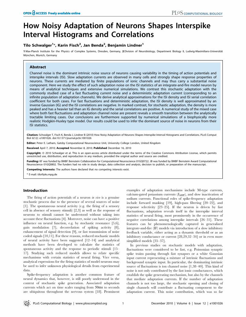
Figure 1. Integrate-and-fire dynamics with adaptation channels. A Channel model: a population of Na independent voltage-gated ionchannels, which can be either in an open or a closed state, mediate an adaptation current through a neuron’s membrane. B PIF model: Subthresholddynamics of the membrane potential V (bottom). The variable V (measured in units of Vth) is reset to a value Vreset~0 after crossing the threshold atV~Vth. Action potentials are not generated explicitely. Instead, the effect of an action potential is captured by the activation function w?(t), whichis set to one in a short time window of 1ms following each threshold crossing of the IF model (middle panel). The adaptation current is proportionalto the fraction of open channels W (top panel). The sample traces were obtained from a simulation of Eq. (35) with Na~1000 channels, white noiseintensity D~0:01V2

th

�ms, adaptation time constant tw~100ms, base current m~0:4Vth=ms and maximal adaptation current b~3Vth=ms. C The

time-dependent firing rate (top) in response to a step stimulus (bottom) is independent of the source of noise (stochastic adaptation – solid line,deterministic adaptation plus white noise – dashed line). The gray line shows the theory given by Eq. (55).doi:10.1371/journal.pcbi.1001026.g001



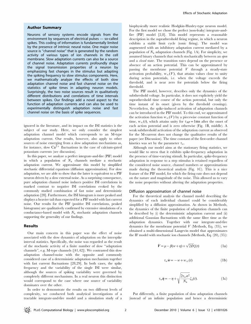
the presence of spikes, which in turn is affected by W (Fig. 2A).

The diffusion approximation of W and the separation of

deterministic and stochastic components are illustrated in Fig. 2B

and 2C, respectively. Although the increments of the continuous

diffusion process have the same (Gaussian) statistics as the original

discontinuous process on a time interval larger than the mean ISI,

the short-time statistics is rather different (Fig. 2A,B). Therefore, it

is not obvious whether the diffusion approximation yields a good

approximation to the ISI statistics, and in particular, how this

approximation depends on the number of channels Na and the

adaptation time constant tw. To clarify this issue, we performed

both simulations based on individual channels (‘‘channel model’’)

and simulations of Eq. (1) (‘‘diffusion model’’). It turned out, that

the diffusion approximation yields a fairly accurate approximation

for the shape of the ISI density, the coefficient of variation and the

serial ISI correlations even for small channel populations.

However, significant deviation were found for higher-order

statistics like the skewness and kurtosis of the ISIH (see next

section).

Interspike interval statistics of the adapting PIF modelThe calculation of the ISI statistics (histogram and serial

correlations) of the PIF model with noise and spike-frequency

adaptation is generally a hard theoretical problem. Here we put

forward several novel approximations for the simple limit cases Eq.

(2) and Eq. (3). For typical adaptation time constants that are

much larger than the mean ISI we found the ISI histogram in the

case of pure white noise (Na??, Eq. (2)) mapping the model to

one without adaptation and renormalized base current ~mm(Methods, Eq. (52)). This corresponds to a mean-adaptation

approximation [18,43–47], because the adaptation variable w(t) is

time-averaged by the linear filter dynamics in Eq. (2b) for tw much

large than the mean ISI (rtw&1). However, this approximation

cannot account for ISI correlations, because any correlations

between ISIs are eliminated in the limit tw?? – in fact, the

reduced model is a renewal model. For this reason, we developed a

novel technique to calculate serial correlations for a PIF neuron

with adaptation and white noise driving, which is valid for any

time constant tw (see Methods).

In the opposite limit of only adaptation fluctuations (D~0, Eq.

(3)), we could calculate analytically the ISI histogram, the skewness

and kurtosis of ISIs as well as the ISI serial correlations by

mapping the problem to one without an adaptation variable but a

colored noise ~gg(t) with renormalized parameters. Specifically, the

IF dynamics for only adaptation channel noise reduces to

_VV~~mm{b~gg ð4aÞ

~tt _~gg~gg~{~ggz

ffiffiffiffiffiffiffiffiffiffi2~tt~ss2

Na

sja(t), ð4bÞ

where the effective parameters are scaled by a common scaling

factor:

~mm~lm, ~tt~ltw, ~ss2~ls2 ð5Þ

with

l~ 1zbtAP

Vth

� �{1

: ð6Þ

As before, a spike is fired whenever V reaches Vth~1,

whereupon the voltage is reset to Vreset~0. We call this model

(Eq. (4)–(6)) the colored noise approximation. For the perfect integrate-

Figure 2. Diffusion approximation of adaptation current. A Sample traces of the integrate-and-fire dynamics with two-state adaptationchannels, Eq. (20), (35) (Na~200 and D~0). The fraction of open channels W (top) exhibits discontinuous jumps with directions that depend on thepresence or absence of a spike as given by the activation function w?(t) (middle panel). B Sample traces of the diffusion model, Eq. (1), with the same1st and 2nd infinitesimal jump moments of W as in the channel model (A). C The fraction of open channels W can be split into the deterministic partw(t), Eq. (1b), corresponding to Na??, and an Ornstein-Uhlenbeck process g(t), Eq. (1c), with a correlation time equal to the adaptation timeconstant (colored noise). The parameters are m~0:4Vth=ms, b~3Vth=ms, tw~100ms.doi:10.1371/journal.pcbi.1001026.g002



and-fire model driven by a weak colored noise, i.e. for the model

described by Eq. (4), analytical expressions for the ISI density and

the serial correlation coefficient are known [48]. In addition to

that, we derived novel analytical expressions for the skewness and

kurtosis of the ISIs (see Methods).

Interestingly, the scaling factor in Eq. (6) has a concrete

meaning in terms of spike-frequency adaptation: l coincides with

the degree of adaptation in response to a step increase of the base

current (see Methods, Eq. (56)).

ISI density. Fig. 3A shows ISI histograms (ISI densities) for

the case of deterministic adaptation. We found, that the ISI

densities can be well described by inverse Gaussian probability

densities with mean Vth=~mm given by Eq. (64) (see Methods). In the

opposite case of stochastic adaptation, the ISI variability solely

depends on the number of slow adaptation channels (Fig. 3B). For

a small channel population (Na~100) the discreteness of the

adaptation W still appears in the ISIH as single peaks that cannot

be averaged out. This is related to realizations of the channel noise

for which the fraction of open channels does not change during the

ISI; realizations for which the fraction changes at least once lead to

the continuous part of the ISI density. In contrast, the diffusion

model yields a purely continuous curve, that looks like a smoothed

version of the ISIH of the model with channel noise. As Na

increases, the discrete peaks in the latter become more and more

dense and insignificant, and the ISIH of the channel model is well

approximated by the diffusion model. Furthermore, the theory for

the colored noise approximation, Eq. (4), coincides well with the

diffusion model, Eq. (1), and hence for sufficiently large Na it also

fits well the ISIH of the channel model.

One central claim of this paper is that ISI histograms of

neurons, for which slow channel noise dominates the ISI

variability, cannot be described by an inverse Gaussian (IG)

distribution in contrast to cases where fast fluctuations dominate.

We recall that the IG distribution yields the ISI histogram for a

PIF model driven by white noise without any (deterministic or

stochastic) adaptation, so a priori we cannot expect that this density

fits any of the cases we consider here. However, as mentioned

above, the ISI density can be captured by an IG for deterministic

adaptation (Fig. 4A,C). In fact, the main effect of a slow adaptation

is to reduce statically the mean input current which is reflected in

our approximation by going from m to ~mm. Slight deviations of the

simulated ISI histogram from the IG can be seen for large intervals

where the simulated density displays a stronger decay than the IG

(Fig. 4C). With adaptation, large intervals are prevented because

for large times (after the last spike) the inhibitory effect of the

adaptation current subsides – a feature that is not present in the

static approximation for the reduced base current which was made

above. Nevertheless, the deviations are small and will be hardly

visible when comparing the IG density to the histogram of limited

experimental data sets.

Figure 3. ISI histograms of a PIF neuron – theory vs. simulation. A ISI densities in the case of deterministic adaptation (Na??) for differentnoise intensities D. Gray bars show the histograms obtained from simulations of Eq. (2); solid lines display the mean-adaptation approximation, Eq.(64) (inverse Gaussian density). B ISI densities in the case of stochastic adaptation (D~0) for different Na as indicated in the panels. The adaptationcurrent was modeled either by the channel model (gray bars), Eq. (20), or by the diffusion model (circles), Eq. (1). The theory, Eq. (69), is displayed as asolid line. Parameters are chosen as in Fig. 2.doi:10.1371/journal.pcbi.1001026.g003



By contrast, the ISI histogram in the case of stochastic

adaptation as illustrated in Fig. 4B and D, possesses a much

stronger peak and decays slower at large ISIs than the IG with the

same mean and variance of the ISI; comparison to the IG density

that has the same mean and mode or the same mode and CV gave

comparably bad fits (data not shown). Instead, the colored noise

approximation as outline above, describes the simulation data

fairly well.

This suggests that both cases – deterministic and stochastic

adaptation – might be distinguishable from the shape of the ISI

histograms even if mean and CV of the ISIs are comparable as for

the data in Fig. 4. To this end, we introduced new measures as and

ae based on the skewness and the kurtosis (excess) of the ISI

distribution that are exactly unity for an IG distribution (see

Methods, Eq. (61) and (62)). Indeed, Fig. 5 reveals that

deterministic and stochastic adaptation are well separated with

respect to the rescaled skewness and kurtosis as and ae. In

particular, these quantities are clearly larger than unity for

stochastic adaptation meaning that the ISI density is more skewed

and more peaked compared to an IG, which confirms our

previous observations. On the other hand, for deterministic

adaptation, as and ae are smaller than unity in accordance with

our previous observations that the tail of the ISI density decays

slightly faster than an IG density.

The rescaled kurtosis reveals also differences between the

channel and the diffusion model. In Fig. 6A, the CV still matches

almost perfectly for both models even at extremely small channel

numbers, where the Gaussian approximation is expected to fail.

This is also remarkable in the light of the discrete structure of the

ISIH for small channel numbers (cf. Fig. 3 for Na~100).

However, in Fig. 6B it becomes apparent that the two models

differ with respect to higher-order measures as ae; for increasing

numbers of channels the differences decrease.

Fig. 5 and 6 also support the colored noise approximation,

which describes the diffusion model quite accurately. This

suggests, that the heavy-tailed and pronouncedly peaked ISIH

Figure 4. Comparison of ISIHs for deterministic vs. stochastic adaptation. A and C – The ISIH obtained from a simulation of thedeterministic adaptation model, Eq. (2), with noise intensity D~0:01V 2

th

�ms can be well described by an inverse Gaussian distribution (dashed line),

Eq. (64). B and D – ISIH for the stochastic adaptation model with Na~200 and D~0. The channel model (gray bars) is more peaked than an inverseGaussian distribution, Eq. (64), with the same mean and CV (dashed line). The ISIH of the diffusion model, (simulation of Eq. (3), circles) is welldescribed by the colored noise approximation, Eq. (69), (solid line). Note the double logarithmic axis in C and D revealing the tail of the distribution.Other parameters as in Fig. 2.doi:10.1371/journal.pcbi.1001026.g004



in the case of stochastic adaptation can be simply explained by

the effect of a long-correlated, colored noise. It is known that

for the related leaky IF model such correlations result in ISIHs

with a large kurtosis [49]. To examine the role of long-range

temporal correlations in shaping the ISI density we analyzed

the dependence of the ISI statistics on the time-scale

separation between adaptation time constant and mean ISI.

This can be quantified by the ratio tw=STiT~rtw, where r and

STiT denote the stationary firing rate and the mean ISI,

respectively.

In the case of stochastic adaptation, we obtained analytical

expressions for as and ae using the colored noise approximation

for weak noise (see Methods). For the following discussion, it

suffices to consider the zeroth order of the weak-noise expansion,

which is given by

a(0)s ~d

1{e{d

d{1ze{dð7Þ

and

a(0)e ~d2 7e{2dz2(d{6)e{dz5

5 d{1ze{dð Þ2: ð8Þ

Figure 5. Shape parameters of the ISIH for deterministic and stochastic adaptation. A Rescaled skewness as for deterministic adaptation(white squares) and for stochastic adaptation (channel model – white circles, diffusion model – black circles, colored noise approximation – graycircles). Different CVs were obtained by varying Na or D. The dashed line depicts the theoretical curve, Eq. (7), and the solid line depicts the semi-analytical result obtained from the moments of the ISI density, Eq. (69), using numerical integration. B The corresponding plot for the rescaledkurtosis ae . The adaptation time constant was tw~100ms. All other parameters as in Fig. 2.doi:10.1371/journal.pcbi.1001026.g005

Figure 6. Comparison of diffusion and channel model. A The coefficient of variation as a function of the number of adaptation channels Na

for the diffusion model (black circles, Eq. (1)), the channel model (white circles, Eq. (20)) and the colored noise approximation (grey circles, Eq. (4)). Thedashed line depicts the theoretical curve Eq. (71) and the solid line depicts the semi-analytical result obtained from the moments of the ISI density,Eq. (69), using numerical integration. B The corresponding curves for the rescaled kurtosis ae . The dashed line represents the theory given by Eq.(114). The time scale separation was rtw~tw=STiT~10. Parameters as in Fig. 2.doi:10.1371/journal.pcbi.1001026.g006



These expressions only depend on the non-dimensional

parameter d~STiT=~tt~(ltwr){1, i.e. on the product of rescaled

adaptation time constant and firing rate. From Eq. (7) and (8), it

can be shown that asw1 and aew1 for rtww0 and that both

quantities converge to unity in the limit twr?0. For tw much

larger than the mean ISI, i.e. when rtw is large, the leading orders

saturate at a(0)s ~2 and a(0)

e ~24=5.

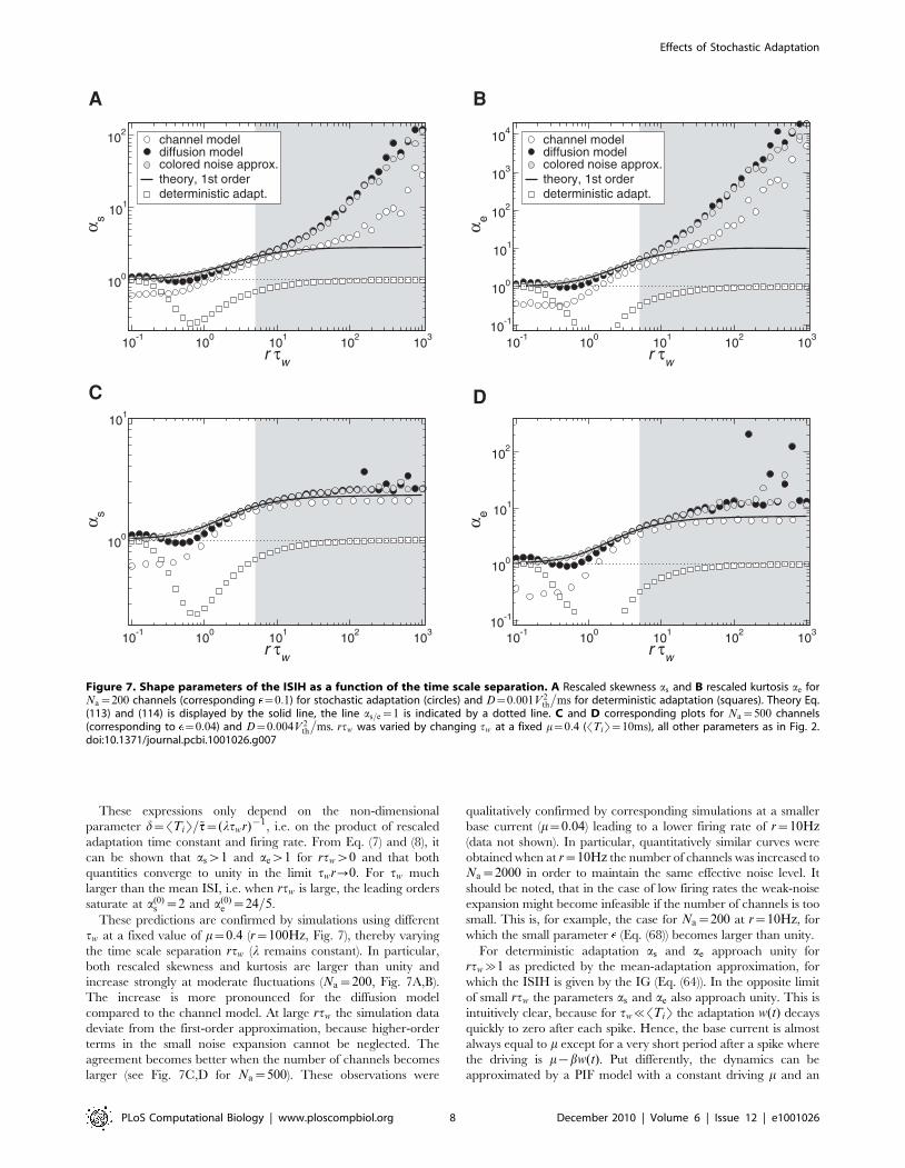
These predictions are confirmed by simulations using different

tw at a fixed value of m~0:4 (r~100Hz, Fig. 7), thereby varying

the time scale separation rtw (l remains constant). In particular,

both rescaled skewness and kurtosis are larger than unity and

increase strongly at moderate fluctuations (Na~200, Fig. 7A,B).

The increase is more pronounced for the diffusion model

compared to the channel model. At large rtw the simulation data

deviate from the first-order approximation, because higher-order

terms in the small noise expansion cannot be neglected. The

agreement becomes better when the number of channels becomes

larger (see Fig. 7C,D for Na~500). These observations were

qualitatively confirmed by corresponding simulations at a smaller

base current (m~0:04) leading to a lower firing rate of r~10Hz(data not shown). In particular, quantitatively similar curves were

obtained when at r~10Hz the number of channels was increased to

Na~2000 in order to maintain the same effective noise level. It

should be noted, that in the case of low firing rates the weak-noise

expansion might become infeasible if the number of channels is too

small. This is, for example, the case for Na~200 at r~10Hz, for

which the small parameter (Eq. (68)) becomes larger than unity.

For deterministic adaptation as and ae approach unity for

rtw&1 as predicted by the mean-adaptation approximation, for

which the ISIH is given by the IG (Eq. (64)). In the opposite limit

of small rtw the parameters as and ae also approach unity. This is

intuitively clear, because for tw%STiT the adaptation w(t) decays

quickly to zero after each spike. Hence, the base current is almost

always equal to m except for a very short period after a spike where

the driving is m{bw(t). Put differently, the dynamics can be

approximated by a PIF model with a constant driving m and an

Figure 7. Shape parameters of the ISIH as a function of the time scale separation. A Rescaled skewness as and B rescaled kurtosis ae forNa~200 channels (corresponding ~0:1) for stochastic adaptation (circles) and D~0:001V2

th

�ms for deterministic adaptation (squares). Theory Eq.

(113) and (114) is displayed by the solid line, the line as=e~1 is indicated by a dotted line. C and D corresponding plots for Na~500 channels(corresponding to ~0:04) and D~0:004V 2

th

�ms. rtw was varied by changing tw at a fixed m~0:4 (STiT~10ms), all other parameters as in Fig. 2.

doi:10.1371/journal.pcbi.1001026.g007



effective reset value Vreset&{btAPv0. In this case, the ISIs are

again distributed according to the IG statistics.

In the intermediate range, where the time scale of the

adaptation is of the same order as the mean ISI, a pronounced

minimum of as and ae is observed in the case of deterministic

adaptation. This is due to the decay of adaptation at such a rate

that large ISIs are suppressed. As a consequence, the tail of the

ISIH decays faster and the ISIH becomes less skewed compared to

an IG. The same qualitative behavior was verified in simulations

at a lower firing rate r~10Hz (data not shown).

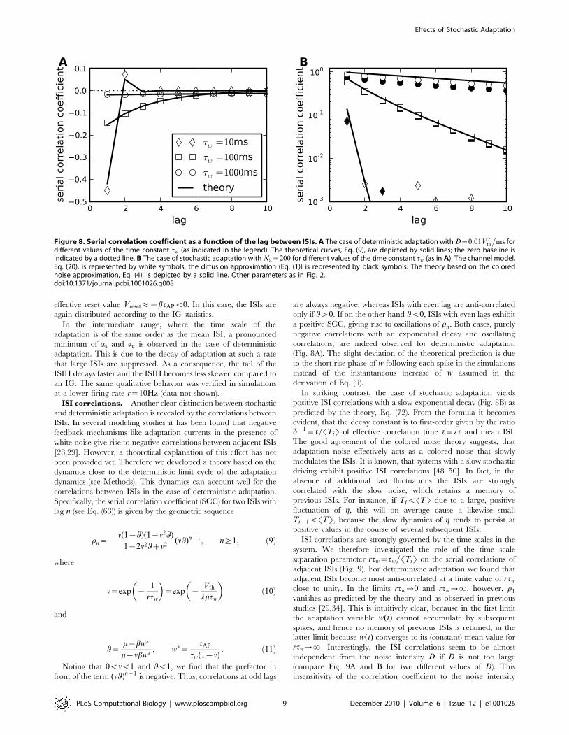
ISI correlations. Another clear distinction between stochastic

and deterministic adaptation is revealed by the correlations between

ISIs. In several modeling studies it has been found that negative

feedback mechanisms like adaptation currents in the presence of

white noise give rise to negative correlations between adjacent ISIs

[28,29]. However, a theoretical explanation of this effect has not

been provided yet. Therefore we developed a theory based on the

dynamics close to the deterministic limit cycle of the adaptation

dynamics (see Methods). This dynamics can account well for the

correlations between ISIs in the case of deterministic adaptation.

Specifically, the serial correlation coefficient (SCC) for two ISIs with

lag n (see Eq. (63)) is given by the geometric sequence

rn~{n(1{q)(1{n2q)

1{2n2qzn2(nq)n{1, n§1, ð9Þ

where

n~exp {1

rtw

� �~exp {

Vth

lmtw

� �ð10Þ

and

q~m{bw�

m{nbw�, w�~

tAP

tw(1{n): ð11Þ

Noting that 0vnv1 and qv1, we find that the prefactor in

front of the term (nq)n{1 is negative. Thus, correlations at odd lags

are always negative, whereas ISIs with even lag are anti-correlated

only if qw0. If on the other hand qv0, ISIs with even lags exhibit

a positive SCC, giving rise to oscillations of rn. Both cases, purely

negative correlations with an exponential decay and oscillating

correlations, are indeed observed for deterministic adaptation

(Fig. 8A). The slight deviation of the theoretical prediction is due

to the short rise phase of w following each spike in the simulations

instead of the instantaneous increase of w assumed in the

derivation of Eq. (9).

In striking contrast, the case of stochastic adaptation yields

positive ISI correlations with a slow exponential decay (Fig. 8B) as

predicted by the theory, Eq. (72). From the formula it becomes

evident, that the decay constant is to first-order given by the ratio

d{1~~tt=STiT of effective correlation time ~tt~lt and mean ISI.

The good agreement of the colored noise theory suggests, that

adaptation noise effectively acts as a colored noise that slowly

modulates the ISIs. It is known, that systems with a slow stochastic

driving exhibit positive ISI correlations [48–50]. In fact, in the

absence of additional fast fluctuations the ISIs are strongly

correlated with the slow noise, which retains a memory of

previous ISIs. For instance, if TivSTT due to a large, positive

fluctuation of g, this will on average cause a likewise small

Tiz1vSTT, because the slow dynamics of g tends to persist at

positive values in the course of several subsequent ISIs.

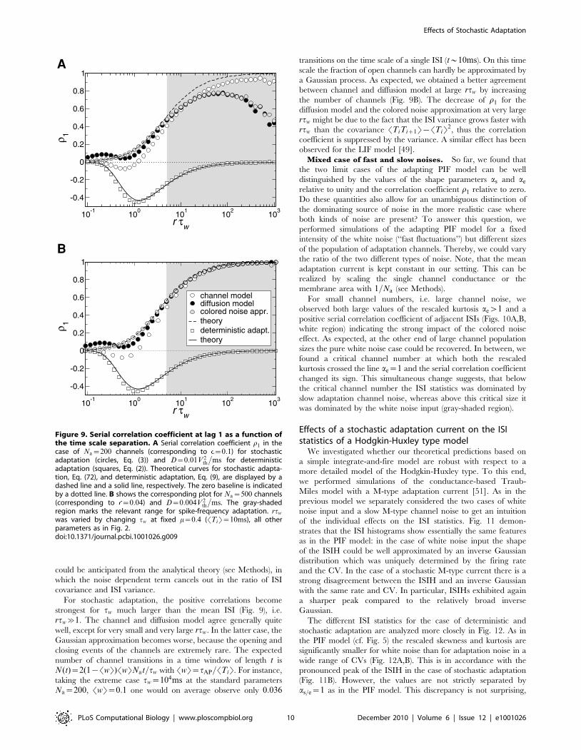
ISI correlations are strongly governed by the time scales in the

system. We therefore investigated the role of the time scale

separation parameter rtw~tw=STiT on the serial correlations of

adjacent ISIs (Fig. 9). For deterministic adaptation we found that

adjacent ISIs become most anti-correlated at a finite value of rtw

close to unity. In the limits rtw?0 and rtw??, however, r1

vanishes as predicted by the theory and as observed in previous

studies [29,34]. This is intuitively clear, because in the first limit

the adaptation variable w(t) cannot accumulate by subsequent

spikes, and hence no memory of previous ISIs is retained; in the

latter limit because w(t) converges to its (constant) mean value for

rtw??. Interestingly, the ISI correlations seem to be almost

independent from the noise intensity D if D is not too large

(compare Fig. 9A and B for two different values of D). This

insensitivity of the correlation coefficient to the noise intensity

Figure 8. Serial correlation coefficient as a function of the lag between ISIs. A The case of deterministic adaptation with D~0:01V2th

�ms for

different values of the time constant tw (as indicated in the legend). The theoretical curves, Eq. (9), are depicted by solid lines; the zero baseline isindicated by a dotted line. B The case of stochastic adaptation with Na~200 for different values of the time constant tw (as in A). The channel model,Eq. (20), is represented by white symbols, the diffusion approximation (Eq. (1)) is represented by black symbols. The theory based on the colorednoise approximation, Eq. (4), is depicted by a solid line. Other parameters as in Fig. 2.doi:10.1371/journal.pcbi.1001026.g008



could be anticipated from the analytical theory (see Methods), in

which the noise dependent term cancels out in the ratio of ISI

covariance and ISI variance.

For stochastic adaptation, the positive correlations become

strongest for tw much larger than the mean ISI (Fig. 9), i.e.

rtw&1. The channel and diffusion model agree generally quite

well, except for very small and very large rtw. In the latter case, the

Gaussian approximation becomes worse, because the opening and

closing events of the channels are extremely rare. The expected

number of channel transitions in a time window of length t is

N(t)~2(1{SwT)SwTNat=tw with SwT~tAP=STiT. For instance,

taking the extreme case tw~104ms at the standard parameters

Na~200, SwT~0:1 one would on average observe only 0:036

transitions on the time scale of a single ISI (t*10ms). On this time

scale the fraction of open channels can hardly be approximated by

a Gaussian process. As expected, we obtained a better agreement

between channel and diffusion model at large rtw by increasing

the number of channels (Fig. 9B). The decrease of r1 for the

diffusion model and the colored noise approximation at very large

rtw might be due to the fact that the ISI variance grows faster with

rtw than the covariance STiTiz1T{STiT2, thus the correlation

coefficient is suppressed by the variance. A similar effect has been

observed for the LIF model [49].

Mixed case of fast and slow noises. So far, we found that

the two limit cases of the adapting PIF model can be well

distinguished by the values of the shape parameters as and ae

relative to unity and the correlation coefficient r1 relative to zero.

Do these quantities also allow for an unambiguous distinction of

the dominating source of noise in the more realistic case where

both kinds of noise are present? To answer this question, we

performed simulations of the adapting PIF model for a fixed

intensity of the white noise (‘‘fast fluctuations’’) but different sizes

of the population of adaptation channels. Thereby, we could vary

the ratio of the two different types of noise. Note, that the mean

adaptation current is kept constant in our setting. This can be

realized by scaling the single channel conductance or the

membrane area with 1=Na (see Methods).

For small channel numbers, i.e. large channel noise, we

observed both large values of the rescaled kurtosis aew1 and a

positive serial correlation coefficient of adjacent ISIs (Figs. 10A,B,

white region) indicating the strong impact of the colored noise

effect. As expected, at the other end of large channel population

sizes the pure white noise case could be recovered. In between, we

found a critical channel number at which both the rescaled

kurtosis crossed the line ae~1 and the serial correlation coefficient

changed its sign. This simultaneous change suggests, that below

the critical channel number the ISI statistics was dominated by

slow adaptation channel noise, whereas above this critical size it

was dominated by the white noise input (gray-shaded region).

Effects of a stochastic adaptation current on the ISIstatistics of a Hodgkin-Huxley type model

We investigated whether our theoretical predictions based on

a simple integrate-and-fire model are robust with respect to a

more detailed model of the Hodgkin-Huxley type. To this end,

we performed simulations of the conductance-based Traub-

Miles model with a M-type adaptation current [51]. As in the

previous model we separately considered the two cases of white

noise input and a slow M-type channel noise to get an intuition

of the individual effects on the ISI statistics. Fig. 11 demon-

strates that the ISI histograms show essentially the same features

as in the PIF model: in the case of white noise input the shape

of the ISIH could be well approximated by an inverse Gaussian

distribution which was uniquely determined by the firing rate

and the CV. In the case of a stochastic M-type current there is a

strong disagreement between the ISIH and an inverse Gaussian

with the same rate and CV. In particular, ISIHs exhibited again

a sharper peak compared to the relatively broad inverse

Gaussian.

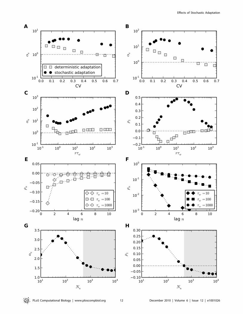
The different ISI statistics for the case of deterministic and

stochastic adaptation are analyzed more closely in Fig. 12. As in

the PIF model (cf. Fig. 5) the rescaled skewness and kurtosis are

significantly smaller for white noise than for adaptation noise in a

wide range of CVs (Fig. 12A,B). This is in accordance with the

pronounced peak of the ISIH in the case of stochastic adaptation

(Fig. 11B). However, the values are not strictly separated by

as=e~1 as in the PIF model. This discrepancy is not surprising,

Figure 9. Serial correlation coefficient at lag 1 as a function ofthe time scale separation. A Serial correlation coefficient r1 in thecase of Na~200 channels (corresponding to ~0:1) for stochasticadaptation (circles, Eq. (3)) and D~0:01V2

th

�ms for deterministic

adaptation (squares, Eq. (2)). Theoretical curves for stochastic adapta-tion, Eq. (72), and deterministic adaptation, Eq. (9), are displayed by adashed line and a solid line, respectively. The zero baseline is indicatedby a dotted line. B shows the corresponding plot for Na~500 channels(corresponding to ~0:04) and D~0:004V2

th

�ms. The gray-shaded

region marks the relevant range for spike-frequency adaptation. rtw

was varied by changing tw at fixed m~0:4 (STiT~10ms), all otherparameters as in Fig. 2.doi:10.1371/journal.pcbi.1001026.g009



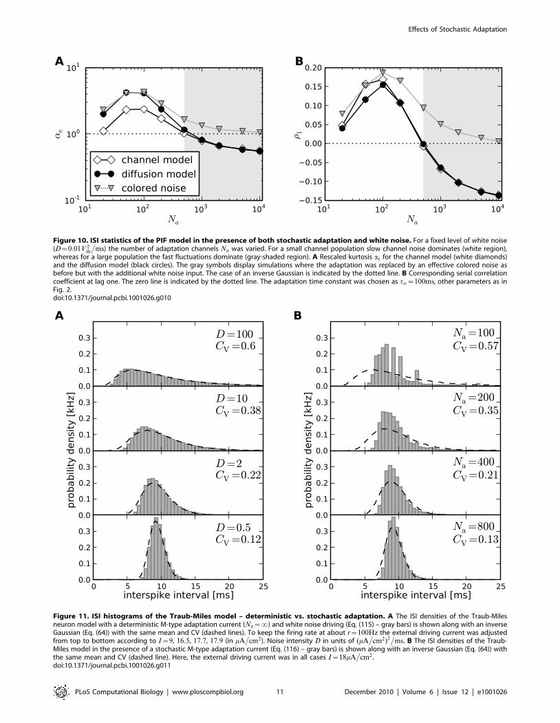
Figure 10. ISI statistics of the PIF model in the presence of both stochastic adaptation and white noise. For a fixed level of white noise(D~0:01V 2

th

�ms) the number of adaptation channels Na was varied. For a small channel population slow channel noise dominates (white region),

whereas for a large population the fast fluctuations dominate (gray-shaded region). A Rescaled kurtosis ae for the channel model (white diamonds)and the diffusion model (black circles). The gray symbols display simulations where the adaptation was replaced by an effective colored noise asbefore but with the additional white noise input. The case of an inverse Gaussian is indicated by the dotted line. B Corresponding serial correlationcoefficient at lag one. The zero line is indicated by the dotted line. The adaptation time constant was chosen as tw~100ms, other parameters as inFig. 2.doi:10.1371/journal.pcbi.1001026.g010

Figure 11. ISI histograms of the Traub-Miles model – deterministic vs. stochastic adaptation. A The ISI densities of the Traub-Milesneuron model with a deterministic M-type adaptation current (Na~?) and white noise driving (Eq. (115) – gray bars) is shown along with an inverseGaussian (Eq. (64)) with the same mean and CV (dashed lines). To keep the firing rate at about r~100Hz the external driving current was adjustedfrom top to bottom according to I~9, 16:5, 17:7, 17:9 (in mA

�cm2). Noise intensity D in units of (mA

�cm2)2

�ms. B The ISI densities of the Traub-

Miles model in the presence of a stochastic M-type adaptation current (Eq. (116) – gray bars) is shown along with an inverse Gaussian (Eq. (64)) withthe same mean and CV (dashed line). Here, the external driving current was in all cases I~18mA

�cm2 .






given that the Traub-Miles dynamics with constant input and

white noise driving does not exactly yield an inverse Gaussian ISI

density but only an approximate one. Importantly, however, the

rescaled kurtosis ae quickly saturates at a finite value in the large

tw limit (albeit not at unity, Fig. 12C). This is markedly different

from the case of stochastic adaptation. In this case, the rescaled

kurtosis increases strongly as it was observed for the PIF model. In

a similar manner, the rescaled skewness also showed this distinct

behavior for stochastic vs. deterministic adaptation, although the

increase of the rescaled skewness was not as strong as for the

rescaled kurtosis (data not shown).

A clear distinction between both cases appears in the serial

correlations of ISIs (Fig. 12D). Similar as in the PIF model, the

case of deterministic adaptation is characterized by negative ISI

correlations at lag one, which are strongest at an intermediate time

scale tw. Furthermore, the case of stochastic adaptation exhibits

positive correlation coefficients r1, which show a maximum at an

intermediate value of tw. This is also in line with the PIF model.

The correlations decay rapidly with the lag for deterministic

adaptation (Fig. 12E) and decay exponentially for stochastic

adaptation (Fig. 12F). As in the PIF model, the exponential decay

is slower for large time constants tw.

Finally, we inspected the case in which both white noise and

slow adaptation noise is present (Fig. 12G,H). As in Fig. 10 for the

PIF model, we fixed the noise intensity of the white noise and

varied the number of adaptation channels Na. In the Traub-Miles

model one finds qualitatively similar curves as in the PIF model. In

particular, the serial correlation coefficient at lag one, shows a

transition from positive to negative ISI correlations at a certain

number of adaptation channels (Fig. 12H). As for the PIF model,

this value can be used to define two regimes – one dominated by

adaptation noise (white region) and another one dominated by

white noise (gray-shaded region). In the adaptation-noise domi-

nated regime the parameter ae is larger than in the white-noise

dominated regime (Fig. 12G).

The observation that key features of the ISI statistics in the

presence of a stochastic adaptation current seem to be conserved

across different models suggests a common mechanism underly-

ing these features. As we saw, this mechanism is based upon the

fact that a stochastic adaptation current can be effectively

described by an independent colored noise. The long-range

temporal correlations of this noise naturally yield positive ISI

correlations and a slow modulation of the instantaneous spiking

frequency. The latter typically involves a large kurtosis due to the

increased accumulation of both short and long ISIs. A significant

amount of colored noise can effect the kurtosis and the ISI

correlations so strongly, that details of the spike generation seem

to be of minor importance. Thus, it becomes plausible that the

spiking statistics of a rather complex neuron model could be

explained by a simple integrate-and-fire model including a

stochastic adaptation current.

Discussion

In this paper, we have studied how a noisy adaptation current

shapes the ISI histogram and the correlations between ISIs. In

particular, we have compared the case of pure stochastic

adaptation with the case of a deterministic adaptation current

and an additional white noise current. Using both a perfect IF

model that is amenable to analytical calculations and a more

detailed Hodgkin-Huxley type model, we found large differences

in the ISI statistics depending on whether noise was mediated by

the adaptation current or originated from other noise sources with

fast dynamics. As regards the ISI histogram, stochasticity in the

adaptation leads to pronounced peaks and a heavy tail compared

to the case of deterministic adaptation, for which the ISI density is

close to an inverse Gaussian. To quantify the shape of ISI

histograms we proposed two measures that allow for a simple

comparison with an inverse Gaussian probability density that has

the same mean and variance. The first one is a rescaled skewness

(involving the third ISI cumulant); the second is a rescaled kurtosis

(involving the fourth ISI cumulant). Both quantities possess the

property that they assume unity for an inverse Gaussian

distribution. If they are larger than unity as in the case of

stochastic adaptation the ISI density is more skewed or

respectively has a sharper peak and a heavier tail than an inverse

Gaussian density with the same variance. If these measures are

smaller than one, the ISI histogram tends to be more Gaussian

like. Most strikingly, we found that for a stochastic adaptation

current the rescaled skewness and kurtosis strongly increase when

the time scale separation of adaptation and spiking becomes large

(tw=STiT&1). By contrast, for a deterministic adaptation current

the rescaled kurtosis saturates close to one in this limit.

Another pronounced difference arises in the ISI correlations.

For a deterministic adaptation current and a white noise driving

one observes short-range anti-correlations between ISIs as

reported previously (e.g. [29]). In contrast, with slow adaptation

noise ISIs exhibit long-range positive correlations. In the presence

of both types of noise, the serial correlation coefficient changes

continuously from positive to negative values when the ratio of

white noise to adaptation noise is increased. The two domains

might be useful in determining the dominating source of noise

from a neural spike train.

Interestingly, the perfect integrate-and-fire model augmented

with an adaptation mechanism predicted all the features seen in

the spiking statistics of the Traub-Miles model with stochastic

adaptation and/or white noise input. This indicates the generality

and robustness of our findings. It also justified the use of the

adapting PIF model as a minimal model for a repetitive firing

neuron with spike-frequency adaptation. It seems, that in the

suprathreshold regime the details of the spike generator are of

minor importance compared to the influence of adaptation and

slow noise.

Figure 12. Comparison of the ISI statistics of the Traub-Miles model – deterministic vs. stochastic adaptation. A Rescaled skewness as

(Eq. (61)) and B rescaled kurtosis ae (Eq. (62)) as a function of the coefficient of variation (CV). For stochastic adaptation (Eq. (116), D~0 – black circles)the number of channels was varied from Na~2000 to Na~80; for deterministic adaptation (Eq. (115), Na~? – gray squares), the noise intensity wasvaried from D~0:1 to D~200. The corresponding inverse Gaussian statistics (Eq. (64)) is indicated by the dotted line. C, D show the rescaled kurtosisand the serial correlation coefficient (Eq. (63)) at lag 1 as a function of the time scale separation rtw . Stochastic adaptation (Na~200) anddeterministic adaptation (D~0:01) are marked as in A,B. E,F The serial correlation coefficient rn as a function of the lag n for different time constantstw in ms as indicated (E deterministic adaptation, F stochastic adaptation; D and Na as in C,D). G The rescaled kurtosis ae in the mixed case at a fixedamount of white noise (D~10) and varying channel numbers Na . H The corresponding values of the serial correlation coefficient at lag one. Theintersection of the r1 curve with the zero line (dotted line) defines the adaptation-noise dominated regime (white region) and the white-noisedominated regime (gray-shaded region). The units of the noise intensities are (mA

�cm2)2

�ms. For stochastic adaptation I~18mA

�cm2 . For

deterministic adaptation I was adjusted to result in a firing rate at around r~100Hz. For D~0 the current I was 18mA�

cm2. With increasing noiseintensity I decreased to I~4mA

�cm2 for D~200.




By means of the PIF model one can theoretically understand the

underlying mechanism leading to the large kurtosis and the

positive ISI correlations in the case of stochastic adaptation. This

rests upon the fact that slow adaptation noise effectively acts as an

independent colored noise with a large correlation time. One can

think of the colored noise as a slow external process that slowly

modulates the instantaneous firing rate or, equivalently, slowly

changes the ISIs in the sequence. Such a sequence of many short

ISIs in a row and a few long ISIs gives rise to a large skewness and

kurtosis and positive serial correlations. In previous works, slow

processes which cause positive ISI correlations were often assumed

to originate in the external stimulus [49,50,52]. Here, we have

shown that an intrinsic process, i.e. the fluctuations associated with

the stochasticity of adaptation, yields likewise positive ISI

correlations. Our finding also provides an alternative explanation

of positive ISI correlations in experimental studies [30,53].

Moreover, in vivo recordings from a looming-sensitive interneuron

in the locust optic lobe have revealed both positive correlations at

large firing rates and negative correlations at low firing rates [23].

Because this neuron exhibits pronounced spike-frequency adapta-

tion an intriguingly simple explanation for these observations

would be the presence of both fast noise and stochastic adaptation

(corresponding to our mixed case). In this case, a large firing rate

could indeed lead to a large effective correlation time of the noise

associated to the adaptation mechanism and thus to positive ISI

correlations.

Spike-frequency adaptation has been ascribed to different

mechanisms (see e.g. [18]), involving for instance, calcium-

dependent potassium currents IAHP [42], slow voltage-dependent

M-type currents IM [41,42] and slow recovery from inactivation of

sodium currents [54]. Here, we chose the M-current as an

example to illustrate the emergence of noise in the adaptation

mechanism. In this specific case, it was the finite number of M-type

potassium channels that gave rise to slow channel noise. For

the other commonly studied adaptation mechanism, the IAHP

[18,23,24,26,29,51], we have to deal with two possible sources of

noise: the finite number of potassium channels NK and fluctuations

of the local Ca2z concentration c. Proceeding in a similar fashion as

for IM, we would obtain IAHP~�ggAHPK(V{EK), with the fraction

K of open potassium channels, obeying

tk_KK~{Kzk?(c)z

ffiffiffiffiffiffiffiffiffiffiffiffi2tks2

k

NK

sjk(t) ð12Þ

tc _cc~{czDX

i

d(t{ti)zffiffiffiffiffiffiffiffiffiffiffi2DCa

pjc(t): ð13Þ

Here, the Gaussian white noises jk and jc approximately

represent the channel noise and the concentration fluctuations due

to stochastic removal of calcium, respectively. The calcium gating

is characterized by the steady-state activation k?(c). For

simplicity, the increase of calcium D caused by an action potential

is assumed to be deterministic. Importantly, however, the channel

dynamics is fast compared to the slow removal of calcium, i.e.

tk%tc. Following [18] the open probability of the potassium

channels k:SKT adiabatically adjusts to c (i.e. k&k?(c)) and the

relationship is roughly linear (i.e. k?(c)!c). Thus, we have

IAHP!(czgk)(V{EK), where the ‘‘channel noise’’ gk possesses a

correlation time tk. If this correlation time is much smaller than

the mean ISI, the channel noise can be approximately treated as a

white noise. But this means, that a PIF neuron with a calcium-

dependent IAHP instead of IM can likewise be approximated by

Eq. (1): the fast channel noise can be included into the white noise

termffiffiffiffiffiffiffi2Dp

j(t) and the slow fluctuations of the calcium

concentration assume the role of the slow adaptation noise g(t).Approximating IAHP again by a voltage-independent current, the

PIF model with IAHP would read

_VV~m{bczffiffiffiffiffiffiffi2Dp

j(t) ð14Þ

tc _cc~{czDX

i

d(t{ti)z

ffiffiffiffiffiffiffiffiffiffiffi2 ~DDCa

qjc(t): ð15Þ

These equations can indeed be put into the form of Eq. (1) by

splitting the deterministic and the noise part of c. This illustrates

that the main results derived in this paper are not specific to a

certain adaptation current, but apply quite generally to any noise

associated to the slow dynamics of adaptation.

The adaptation currents IM and IAHP have been distinguished

with respect to their ability to synchronize coupled neurons [51]

and regarding the influence on neural coding [55]. The difference

consists in whether the current is activated solely by spikes as in the

case of IAHP or whether it is also activated by subthreshold

voltages as for IM. For the sake of clarity, we have set the

activation function w?(t) of the M-type adaptation current in the

PIF model equal to zero at subthreshold voltages, i.e. between

spikes (Eq. (25)). Thus, the adaptation current in the PIF model,

unlike the M-current, was only activated during action potentials.

It is, however, easy to show that the results of this paper are

unchanged if subthreshold activation is allowed. For simplicity, let

us consider the extension that in-between spikes the steady-state

activation function w? is equal to the value v1, i.e. instead of

Eq. (25), (26) (see Methods) we have

w?(t)~1 ti�ƒtvti�ztAP

else

�ð16Þ

~ z(1{ )X

i

h(t{ti)h(tiztAP{t): ð17Þ

This only increases the mean adaptation to

SwT~Sw?(t)T~ z(1{ )rtAP (cf. Eq. (37)). Similarly, the

variance changes according to s2~SwT{SwT2 (cf. Eq. (40) in

Methods). As a result, the effective base current is now given by

~mm~l(m{b ) ð18Þ

with the new scaling factor

l~ 1z(1{ )btAP

Vth

� �{1

: ð19Þ

The colored noise approximation can be carried out in an

analogous manner yielding the same result Eq. (4) (again with

~tt~ltw, ~ss2~ls2, but the new scaling factor l, Eq. (19)). Thus, it

can be expected that in the presence of subthreshold activation of

w(t) the colored noise effect (i.e. pronounced peak of ISIH,

positive ISI correlations) in the case of stochastic adaptation is



preserved. Furthermore, l still serves as the degree of adaptation,

i.e. the ratio of steady-state to initial gain when a step current is

applied.

The analytical calculation of higher-order statistics in the presence

of adaptation is a fundamental theoretical problem, which has

been largely ignored so far (for a recent exception see [37]). Here,

we succeeded to provide explicit expressions for the ISI histogram

and their serial correlations for both white noise driving and noise

in the adaptation dynamics. This was achieved by analyzing a

spike generator and a channel model that are as simple as possible.

There are certainly a lot of details that can be modeled in a more

realistic way. For instance, it is known that the M-channel kinetics

is governed by several time scales and more than two internal

states [56]. Furthermore, channels might not be strictly indepen-

dent, but channel clusters might exhibit cooperative behavior [57].

The latter case, would actually increase the level of channel noise

compared to the case of independent channels, i.e. cooperativity

would contribute to stochastic adaptation.

For many neurons physiological details like the number of ion

channels are hard to obtain directly from experiments. Instead

given the spike train statistics of a neuron, our study could be

useful to judge whether M-channels or other adaptation

mechanisms could potentially contribute to the neuronal variabil-

ity. Furthermore, it is not impossible to think of experiments, in

which the number of adaptation channels is reduced (e.g. by the

mild application of a channel blocker) and thus the effects of

stochastic adaptation is affected in a controlled way. Another

possibility to test our predictions would be to vary the firing rate of

the neuron by increasing or decreasing the input current. In this

way, the time scale of spiking would change relative to the time

scale of adaptation and, thus, the colored noise effect of adaptation

noise could be enhanced or attenuated, respectively.

Channel noise can crucially influence neural firing especially in

the absence of synaptic input [58,59]. This could be particularly

relevant for the irregular discharge patterns of certain receptor

cells. So far, channel noise has been studied mostly in the context

of stochastic Naz and Kz channel gating involved in the spike

generation itself. These channels are considered to be fast. Because

we were mainly interested in the effect of slow adaptation channels

compared to fast fluctuations resulting from fast ion channels or

synaptic activity, we lumped all fast noise sources into an

unspecified additive white noise source. This is certainly a

simplification; e.g. it has been shown in experiments that voltage

noise due to Naz channels depends on the mean voltage itself

[39,40]. More detailed models of the various sources of noise are

worth the efforts in future investigations. However, we do not

expect that such sophisticated models would change our results

qualitatively, because they mainly hinge upon the presence or

absence of long time scales.

Realistic numbers of M-type channels per neuron are difficult to

estimate and the numbers used in this paper must be seen as a

tuning parameter for the channel noise intensity. Channel

densities of the M-type have been estimated to be of the order

of one functional channel per 4mm2 [60]. Assuming a spherical

cell with a diameter of 10mm one obtains of the order of 100channels. Thus, the channel numbers used in this study (Na~20–

1000) seem to be reasonable; and hence the M-current could be a

potential source of fluctuations.

The diffusion approximation for the stochastic dynamics of ion

channel populations (also known as Langevin or Gaussian

approximation) has been studied by several authors [38,61–64]

(see also [65] in the context of chemically reacting particles). Here,

we have shown how one can map the stochastic dynamics of a

population of ion channels with negative feedback to the

macroscopic current dynamics plus an additive colored noise

(see [38] for a related treatment). In other words, the dynamics

could be reduced to an analytically accessible Langevin equation

for voltage and adaptation. In particular, we investigated the effect

of the diffusion approximation on the statistics of interspike

intervals and found a fairly good agreement with the channel

model, despite the small number of channels. This seems

surprising, given that for a typical parameter set – Na~200, open

probability SwT*0:1 and tw~100ms – one expects only 1:8closing transitions (between spikes) and 0:2 open transitions

(during action potentials) per millisecond. Apparently, on the

time scale of 1 ms the number of transition events is not Gaussian

distributed. However, we found that the main effect of the channel

noise consists in a slow modulation of the instantaneous firing rate

on the large time scale of ~tt~lt, whereas high-frequency

components of the noise are of minor importance. Thus, on

relevant time scales of the order of 10–100 ms the average number

of transitions is much larger and a Gaussian approximation seems

to be reasonable.

Spike-frequency adaptation has been commonly studied with

regard to its mean effect on the firing rate [18,43–46]. It has been

shown that these effects can be exhaustingly analyzed using a

universal firing rate model [18]. In this paper, however, it became

evident that higher-order statistics and fluctuation effects may

differ and may be used to distinguish different kinds of noise

sources.

Methods

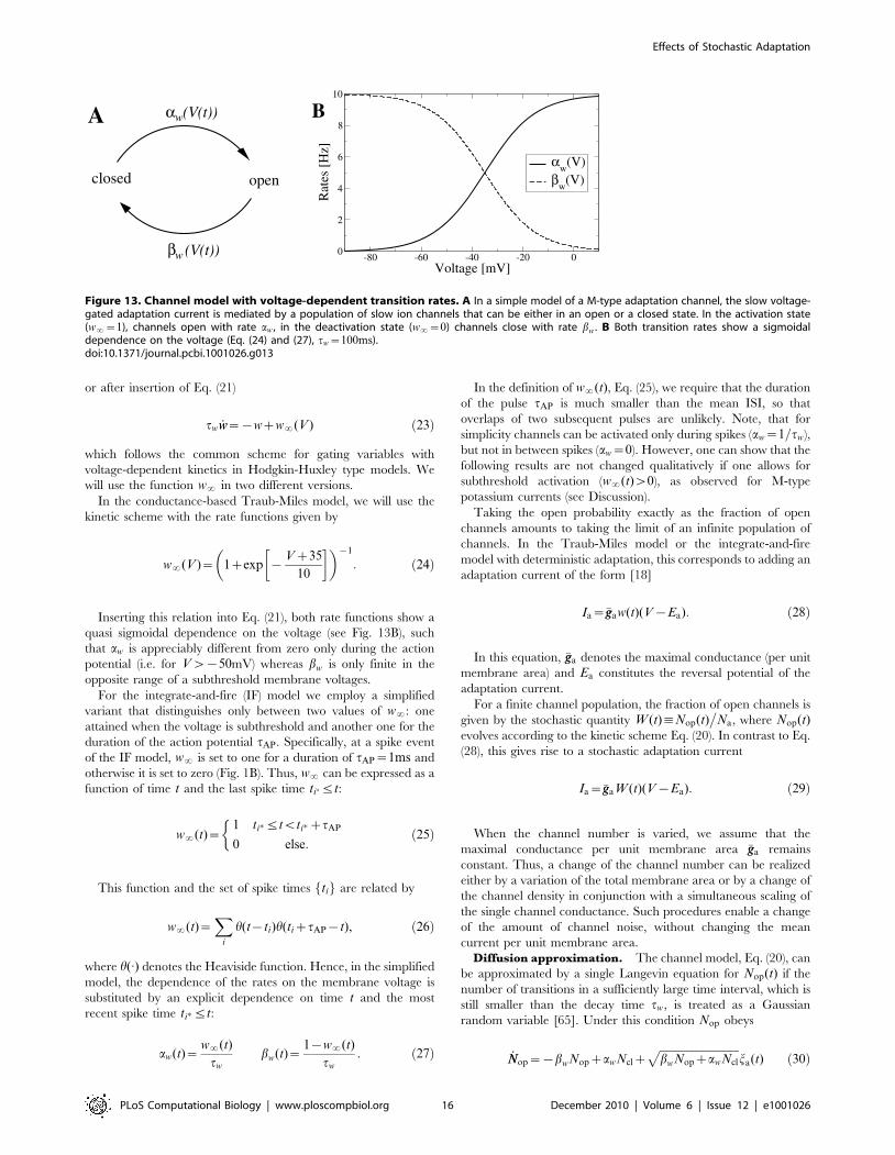
Model for the stochastic adaptation currentTo analyze the slow, voltage-dependent adaptation channels in

a simple setup we consider a population of Na independent ion

channels that reside in an open or a closed state. For each channel,

we thus have the simple reaction kinetics shown in Fig. 13A.

For Na channels, one can either perform Na independent

simulations of one two-state process or one simulation with Na

states where the number of open channels Nop can be increased or

decreased by one:

Nop

awNclNopz1 ð20aÞ

Nop

bwNopNop{1: ð20bÞ

Here, Ncl(t)~Na{Nop(t) denotes the number of closed

channels. The rates aw and bw for the transitions between the

closed and open state can be related to the (voltage-dependent)

kinetics of a typical gating variable by choosing

aw(V )~w?(V )

tw

bw(V)~1{w?(V )

tw

: ð21Þ

Therein, w?(V ) is the steady-state open probability of a single

channel when the membrane potential is clamped at V and tw sets

the time scale of the channel kinetics. Note, that both w?(V ) and

tw are accessible from experiments. The master equation for the

open probability of the two-state model reads

_ww~aw(V )(1{w){bw(V)w ð22Þ



or after insertion of Eq. (21)

tw _ww~{wzw?(V ) ð23Þ

which follows the common scheme for gating variables with

voltage-dependent kinetics in Hodgkin-Huxley type models. We

will use the function w? in two different versions.

In the conductance-based Traub-Miles model, we will use the

kinetic scheme with the rate functions given by

w?(V )~ 1zexp {Vz35

10

� �� {1

: ð24Þ

Inserting this relation into Eq. (21), both rate functions show a

quasi sigmoidal dependence on the voltage (see Fig. 13B), such

that aw is appreciably different from zero only during the action

potential (i.e. for Vw{50mV) whereas bw is only finite in the

opposite range of a subthreshold membrane voltages.

For the integrate-and-fire (IF) model we employ a simplified

variant that distinguishes only between two values of w?: one

attained when the voltage is subthreshold and another one for the

duration of the action potential tAP. Specifically, at a spike event

of the IF model, w? is set to one for a duration of tAP~1ms and

otherwise it is set to zero (Fig. 1B). Thus, w? can be expressed as a

function of time t and the last spike time ti�ƒt:

w?(t)~1 ti�ƒtvti�ztAP

0 else:

�ð25Þ

This function and the set of spike times ftig are related by

w?(t)~X

i

h(t{ti)h(tiztAP{t), ð26Þ

where h(:) denotes the Heaviside function. Hence, in the simplified

model, the dependence of the rates on the membrane voltage is

substituted by an explicit dependence on time t and the most

recent spike time ti�ƒt:

aw(t)~w?(t)

tw

bw(t)~1{w?(t)

tw

: ð27Þ

In the definition of w?(t), Eq. (25), we require that the duration

of the pulse tAP is much smaller than the mean ISI, so that

overlaps of two subsequent pulses are unlikely. Note, that for

simplicity channels can be activated only during spikes (aw~1=tw),

but not in between spikes (aw~0). However, one can show that the

following results are not changed qualitatively if one allows for

subthreshold activation (w?(t)w0), as observed for M-type

potassium currents (see Discussion).

Taking the open probability exactly as the fraction of open

channels amounts to taking the limit of an infinite population of

channels. In the Traub-Miles model or the integrate-and-fire

model with deterministic adaptation, this corresponds to adding an

adaptation current of the form [18]

Ia~�ggaw(t)(V{Ea): ð28Þ

In this equation, �gga denotes the maximal conductance (per unit

membrane area) and Ea constitutes the reversal potential of the

adaptation current.

For a finite channel population, the fraction of open channels is

given by the stochastic quantity W (t):Nop(t)�

Na, where Nop(t)evolves according to the kinetic scheme Eq. (20). In contrast to Eq.

(28), this gives rise to a stochastic adaptation current

Ia~�ggaW (t)(V{Ea): ð29Þ

When the channel number is varied, we assume that the

maximal conductance per unit membrane area �gga remains

constant. Thus, a change of the channel number can be realized

either by a variation of the total membrane area or by a change of

the channel density in conjunction with a simultaneous scaling of

the single channel conductance. Such procedures enable a change

of the amount of channel noise, without changing the mean

current per unit membrane area.

Diffusion approximation. The channel model, Eq. (20), can

be approximated by a single Langevin equation for Nop(t) if the

number of transitions in a sufficiently large time interval, which is

still smaller than the decay time tw, is treated as a Gaussian

random variable [65]. Under this condition Nop obeys

_NNop~{bwNopzawNclzffiffiffiffiffiffiffiffiffiffiffiffiffiffiffiffiffiffiffiffiffiffiffiffiffiffiffiffiffibwNopzawNcl

pja(t) ð30Þ

Figure 13. Channel model with voltage-dependent transition rates. A In a simple model of a M-type adaptation channel, the slow voltage-gated adaptation current is mediated by a population of slow ion channels that can be either in an open or a closed state. In the activation state(w?~1), channels open with rate aw , in the deactivation state (w?~0) channels close with rate bw . B Both transition rates show a sigmoidaldependence on the voltage (Eq. (24) and (27), tw~100ms).doi:10.1371/journal.pcbi.1001026.g013



with Ncl~Na{Nop and Gaussian white noise ja(t), with

Sja(t)ja(t’)T~d(t{t’). Dividing Eq. (30) by Na and using Eq.

(27) we obtain a Langevin equation for the fraction of open

adaptation channels W ,

tw_WW~{Wzw?(t)z

ffiffiffiffiffiffiffiffiffiffiffiffiffiffiffiffiffiffiffiffiffiffiffiffiffiffiffiffiffiffiffiffiffiffi2tws2(W ,w?(t))

Na

sja(t) ð31Þ

where s2(W ,w?(t)) is given by

s2(W (t),w?(t))~1

2½1{w?(t)�Wzw?(t)½1{W �f g: ð32Þ

Furthermore, a separation of the adaptation into a deterministic

and a stochastic part, W~wzg, will be useful for the inter-

pretation of our results. In these new variables Eq. (31) can be

rewritten as two equations:

tw _ww~{wzw?(t) ð33Þ

tw _gg~{gz

ffiffiffiffiffiffiffiffiffiffiffiffiffiffiffiffiffiffiffiffiffiffiffiffiffiffiffiffiffiffiffiffiffiffiffiffiffiffiffi2tws2(wzg,w?(t))

Na

sja(t): ð34Þ

Note that Eq. (1), which will be our final diffusion model,

also involves the additive-noise approximation presented

below.

Perfect integrate-and-fire model with adaptationThe perfect integrate-and-fire (PIF) model [2] constitutes a

minimal model for a neuron possessing a stable limit cycle. In this

model the subthreshold voltage is determined by the equation

_VV~m{bWzffiffiffiffiffiffiffi2Dp

j(t), ð35Þ

where m~I0=Cm and {bW are proportional to the base current

I0 and adaptation current Ia(t), respectively; Cm is the membrane

capacitance and the scaling factor for the adaptation current reads

b~�gga(E0{Ea)=Cm. Here, we used an effective-time-constant

approximation [66], where we substituted in Eq. (29) V by the

average voltage E0~SVT to obtain a voltage-independent

adaptation current [18].

The last term in Eq. (35) represents fast Gaussian input fluctuations

of intensity D and correlation function Sj(t)j(t’)T~d(t{t’) (here

and in the following, the angular brackets denote an ensemble

average). The model Eq. (35) is complemented by the fire-and-reset

rule: upon reaching the threshold Vth a spike is elicited and V is reset

to Vreset, VresetvVth. Because Eq. (35) is invariant with respect to a

constant shift in V , we can choose the reset value as the origin, i.e.

Vreset~0. The threshold crossing events define the spike times ti,

i~0,1,…of the PIF model.

It is a feature of the PIF model that the firing rate is directly

proportional to a constant driving current and independent of the

noise. However, even for the slowly varying driving current

m{bW (t) in Eq. (35), one can define an instantaneous firing rate

�rr(t)~m{bW

Vth, ð36Þ

which can be seen as the slowly varying firing rate that is obtained

by averaging the spike train over the time scale tw of the

adaptation. Averaging over time scales much larger than tw yields

a constant firing rate r, because the process is stationary. Thus, the

(stationary) firing rate can be obtained by averaging Eq. (36),

which gives r~ m{bSwTð Þ=Vth. On the other hand, the firing rate

is related to the mean fraction of open channels by averaging Eq.

(33):

SwT~Sw?(t)T~rtAP: ð37Þ

Solving for r yields

r~lm

Vth, ð38Þ

where l~(1zbtAP=Vth){1.

Additive-noise approximation. The noise term in Eq. (31)

or (34) is multiplicative, because both arguments of the noise

strength s2 W ,w?(t)ð Þ depend on the dynamical variables. For

slow adaptation, rtw&1, and large Na, however, the relative

fluctuations of s2(W ,w?(t)) are small and, hence, s2 can be

treated as constant (additive-noise approximation). This can be

seen as follows: The rapid changes of s2(W ,w?(t)) due to the

switchings of w?(t) between 0 and 1 on the time scale of the mean

ISI are averaged out by the linear filter dynamics Eq. (34) if

rtw&1. Thus, in Eq. (32) w?(t) can be replaced by its local

average tAP�rr(t). Because of Eq. (36), s2 can therefore be written as

a quadratic function of W . As explained below (Sec. ‘‘Colored

noise approximation’’), the variance of W is ls2�

Na. Thus, using

SWT~SwT and SW 2T&lSs2T=NazSwT2 the mean of s2 can

be self-consistently determined. It can be shown that

Ss2T~ SwT{SwT2 �

1{D

(1zD)Na

� �ð39Þ

&SwT{SwT2 ð40Þ

~rtAP{(rtAP)2, ð41Þ

where D~btAP=Vth and r is given by Eq. (38). In the second line

we neglected the term that depends on N{1a , because for large

Na it is much smaller than unity. Similarly, the variance of s2

can be calculated neglecting terms that are third and forth order in

W . As a result, we obtain Var s2�

~(1{D)2

4(1zD)NaSwTzO SwT2

.

The relative fluctuations of the noise intensity are given byffiffiffiffiffiffiffiffiffiffiffiffiffiffiffiVar s2½ �

p .Ss2T. Inserting the expressions for mean and variance

of s2 to first order in SwT, we find that the additive-noise

approximation s(W ,w?(t))&Ss2T is roughly valid if

j1{Dj2ffiffiffiffiffiffiffiffiffiffiffiffiffiffiffiffiffiffiffiffiffiffiffiffiffiNatAPm=Vth

p %1: ð42Þ

For the standard parameter set used in this paper, D~3,

m~0:4, tAP~1, Vth~1, we find the condition 1� ffiffiffiffiffiffiffiffiffiffiffiffi

0:4Na

p%1. For

instance, for Na~200 the relative fluctuations of s2 are 11%.



Non-dimensional form. It is useful to regard a non-

dimensional form of Eq. (35). To this end, we measure

henceforth voltages in units of Vth and time in units of tw, i.e.

we introduce the variables VV~V=Vth and tt~t=tw. Furthermore,

we will use the adaptation variable A~twb

Vth

W . Then Eq. (31) and

(35) can be rewritten as

_VVVV~mm{Az

ffiffiffiffiffiffiffi2DD

pj(tt) ð43Þ

_AA~{Aza? (tt)zffiffiffiffiffiffiffi2ss2p

ja (tt), ð44Þ

where the firing threshold is VVth~1 and the adaptation feedback is

given by the function

a? (tt)~twb

Vth

w?(twtt)&DX

i

d(tt{tti): ð45Þ

The dynamics of the PIF model is completely determined by the

four non-dimensional parameters

mm~twm

Vth, D~

btAP

Vth, DD~

twD

V2th

ð46Þ

and

ss2~t2

wb2Ss2TV2

thNa

~Dmt2

w

(1zD)V2thNa

b{D

1zDm

� �: ð47Þ

In the last step, Eqs. (38) and (41) were used. The second term of

ss2 can be neglected, because it arises from the small term (rtAP)2

in Eq. (41). In fact, rtAP is the ratio between the spike duration and

the mean ISI, which can be assumed to be small. Thus, the

channel noise intensity is approximately

ss2&Dbmt2

w

(1zD)V2thNa

: ð48Þ

Again, the adaptation variable A can be written as the sum of a

deterministic part a(t) and a stochastic part ga(t), satisfying the

equations

_aa~{aza? (tt), _gga~{gazffiffiffiffiffiffiffi2ss2p

ja (tt): ð49Þ

In accordance with Eq. (37), the mean adaptation is

proportional to the firing rate [18],

SAT~SaT~D:rr, ð50Þ

where rr is the firing rate in units of t{1w .

Mean adaptation approximation. In the case of

deterministic adaptation (Na??), the membrane potential is

driven by the current mm{a and by white noise. If the firing rate of

the neuron is large compared to the decay rate of the adaptation

current, i.e. if rr&1, the trace a(t) is effectively smoothed by the

linear filter equation Eq. (49). As a consequence, the relative

deviations of a(t) from its mean value SaT are small, so that the

replacement a(t)?SaT yields a good approximation for

calculating the ISI density. In the PIF model, SaT can be self-

consistently determined from Eq. (50), because for the constant

input current mm{SaT the firing rate of the PIF model is simply

given by rr~mm{SaT. Solving for the firing rate yields

rr~lmm ð51Þ

with l~(1zD){1. Thus, the mean adaptation approximation of

the PIF model reads

_VVVV~lmmz


pj(tt): ð52Þ

Colored noise approximation. In the case of stochastic

adaptation (D~0) one can approximate the adaptation variable

A~azga by an effective colored noise. If the adaptation is slow,

i.e. rr&1, the spike train looks almost periodic at small time scales

with a slowly varying frequency �rr(tt)~mm{A (in units of 1=tw),

because of the absence of fast fluctuations. As a result, the

instantaneous firing frequency �rr(tt) can be well estimated already

by averaging over a few spikes. Because the linear filter in Eq. (49)

averages a? (tt) on time scales of the order of 1, the dynamics of A

is retained if in Eq. (44) a?(t) is replaced by its slowly varying

average D:�rr(t):

_AA~{AzD(mm{A)zffiffiffiffiffiffiffi2ss2p

ja (tt)

Multiplication with l~(1zD){1 yields

l _AA~{AzDlmmzffiffiffiffiffiffiffiffiffiffiffiffi2l2ss2

pja(tt):

Finally, we perform the variable transformation gg~A{Dlmm, so

that we obtain a colored noise driven PIF neuron model

_VVVV~lmm{gg ð53aÞ

l _gggg~{ggzffiffiffiffiffiffiffiffiffiffiffiffi2l2ss2

pja(tt): ð53bÞ

As can be seen from Eq. (53a), the stationary firing rate for

stochastic adaptation is again given by Eq. (51).

Nonstationary firing rate. If the stimulus depends on time,

i.e. if mm~mm(tt), the firing rate is a function of time as well. Here,

the firing rate rr(tt) is understood in the sense of an ensemble

average or peri-stimulus histogram. In the PIF model, such a firing

rate is given by the ensemble average of the instantaneous rate

�rr~mm{A, i.e. rr(tt)~mm(tt){SA(tt)T. The ensemble average of A(tt)can be obtained by averaging Eq. (44). Solving for the firing rate

yields

rr(tt)~mm(tt) 1{D

ð tt

{?exp {

tt{t’l

� �mm(t’)mm(tt)

dt’

" #: ð54Þ

As an example, let us consider a step of the base current at time

tt� such that mm(tt)~mm0zh(tt{tt�)mm1. In this case, the time-

dependent firing rate reads



rr(tt)~lmm(tt) 1zDmm1

mm0zmm1

exp {tt{tt�

l

� �h(tt{tt�)

� �: ð55Þ

This represents exactly the exponential decay of the firing rate

in response to a step stimulus, which is typical for spike-frequency

adaptation. Eq. (55) has been used in Fig. 1C.

The dynamical response to a step stimulus yields an interesting

interpretation of the scaling factor l: from Eq. (55) one finds that

l~rr?{rr0

rr�{rr0, ð56Þ

which is the ratio of firing rate increases after adaptation to the

increase directly after stimulus onset. In Eq. (56), rr0~lmm0,

rr�~rr(t�z) and rr?~l(mm0zmm1) are the firing rates before stimulus

onset, directly after the step and at tt~?, respectively. Thus, lquantifies the ‘‘percentage adaptation’’ or the ‘‘degree of

adaptation’’ [26].

Statistical measures and known expressions for the PIFmodel

In the following, Ti~ti{ti{1 denotes the interspike intervals

(ISIs), i.e. the intervals between adjacent spikes, and TTi~Ti=tw are

the corresponding ISIs in units of the adaptation time constant. The

statistics of ISIs can be characterized by different measures. A single

interval TTi is distributed according to the probability density

P(TT)~Sd(TT{TTi)T, i.e. the normalized ISI histogram. The shape

of the ISI density can be characterized using the cumulants. The first

cumulant equals the mean ISI and the inverse of the firing rate rr,

k1~STTiT~1

rr: ð57Þ

The second cumulant equals the variance and is related to the

coefficient of variation (CV), which is a measure of ISI variability:

k2~STT2i T{STTiT2, CV~

ffiffiffiffiffik2p

k1: ð58Þ

We further consider the third cumulant, which is related to the

skewness cs of the ISI distribution, defined as

k3~STT3i T{3STTiTSTT2

i Tz2STTiT3, cs~k3

k3=22

, ð59Þ

and the fourth cumulant, which determines the kurtosis (or excess)

ce of the ISI distribution. It is defined as

k4~STT4i T{3STT2

i T2{4STTiTSTT3i Tz12STTiT2STT2

i T{6STTiT4,

ce~k4

k22

:ð60Þ

Roughly speaking, the kurtosis indicates how much of the

variability is due to events that strongly deviate from the mean

value. For instance, a unimodal ISI density with a heavier tail

compared to another ISI density with the same CV, tends to

exhibit a larger kurtosis. This is typically accompanied by a more

pronounced peak close to the mean value to balance the heavy tail.

In this paper, we want to compare the ISI density with an

inverse Gaussian probability density serving as a reference statistic.

For an inverse Gaussian ISI distribution (see below) one observes

that the skewness is proportional to the CV and the kurtosis scales

like the squared CV. This suggests to introduce rescaled versions

of the skewness and the kurtosis as follows:

as~cs

3CV

~k1k3

3k22

ð61Þ

and

ae~ce

15C2V

~k2

1k4

15k22

: ð62Þ

By defining the rescaled skewness and kurtosis in this manner,

we obtain measures that are identical to unity for an inverse

Gaussian ISI density. For larger (smaller) values, the ISI density is

respectively more (less) skewed and more (less) peaked compared

to an inverse Gaussian density. This procedure is somewhat

analogous to the definition of the CV, for which the Poisson

process serves as a reference for the ISI variability with CV~1.

Furthermore, we consider the correlations among ISIs as

quantified by the serial correlation coefficient [67]:

rn~STTiTTiznT{STTiT2

STT2i T{STTiT2

, ð63Þ

where due to stationarity the expression does not depend on the

integer i, i.e. on the position in the sequence of ISIs. Alternatively,

the averages involved in Eq. (63) can also be taken along the

sequence (. . . ,TTi{1,TTi,TTiz1, . . .).For the adapting PIF model, the two limit cases that are

considered in this paper could be reduced to simplified models, for

which analytical results are partly known. Firstly, in the case of

deterministic adaptation, i.e. Na??, the ISI density can be

approximately described by the first-passage-time density of a

biased Brownian motion described by Eq. (52) (mean adaptation

approximation). A classical result for this purely white noise driven

PIF neuron with a constant drift lmm is that the ISI density is given

by the so-called inverse Gaussian [2]

PWN(TT)~1ffiffiffiffiffiffiffiffiffiffiffiffiffiffiffi

4pDDTT3p exp {

(TT{STTiT)2

4DDSTTiT2TT

" #: ð64Þ

This distribution has a mean

STTiT~rr{1~(lmm){1 ð65Þ

and a CV

CV~


lmm

s: ð66Þ

Furthermore, by construction we have

as,WN~ae,WN~1: ð67Þ



The mean adaptation approximation would wrongly predict that

the ISIs are uncorrelated. The reason is that in the PIF model driven

by only white Gaussian noise any memory of the ISI history is erased

upon reset. A better account of ISI correlations is given below.

Secondly, the case of stochastic adaptation can be reduced to a

PIF neuron driven by a reduced base current lmm and a colored

noise with correlation time l and variance lss2 (Ornstein-

Uhlenbeck process, see Eq. (53)). In the case of a weak colored

noise, it is useful to define the small parameter

~ss2

lmm2&

b2tAP

VthNam: ð68Þ

For %1 an approximation for the ISI density is given by [48]

POU(TT)~1

2lffiffiffiffiffiffiffiffiffiffiffi4p c3

1

q exp {(TT{STTiT)2

4 l2c1

" #

½(STTiT{TT)c2z2c1l�2

2c1l2{ (c2

2{2c1e{TT=l)

( ),

ð69Þ

with c1(TT)~TT=lze{TT=l{1, c2(TT)~1{e{TT=l and mean ISI

STTiT. For TT%l, i.e. for ISIs much smaller than the correlation time

of the colored noise, the expression for POU(TT) reduces to [50]:

POU(TT)~STTiT2ffiffiffiffiffiffiffi2pp

TT3exp {

(TT{STTiT)2

2 TT2

" #, TT%l: ð70Þ

Although this formula captures the ISI density at small ISIs, it is

of limited use, because the second and higher ISI moments

diverge. Throughout the paper we have therefore used the full

expression Eq. (69). The mean ISI and the firing rate do not

depend on the noise statistics, in fact they are equal to the white

noise case, Eq. (65), as shown below (derivation of the ISI

cumulants). The squared CV can be obtained to second order in

[48] using the methods presented below:

C2V~

2

d1{

1{e{d

d

� �z 2 e{dz

(1{e{d)(1{2e{d)

d

� �� , ð71Þ

with d~(l2mm){1~STTiT�

l. Similarly, the rescaled skewness and

kurtosis are derived for weak colored noise below. Finally, the

serial correlation coefficient can be computed analytically for weak

noise [48] (nw0):

rn~4

C2Vd2

e{nd sinh2 d

2

� �z 2e{nd sinh2 (d)�

z(nd{3) sinh2 d

2

� �{

d

2sinh(d)

��:

ð72Þ

Serial correlation coefficient of adaptive PIF neurondriven by white noise

Here we derive an expression for the serial correlation

coefficient of a PIF neuron with deterministic adaptation current

and white noise driving. We consider the following subthreshold

dynamics

_VVVV~mm{az


pj(tt) ð73Þ

_aa~{azDX

i

d(tt{tti) ð74Þ

augmented with the usual reset rule for VV at the spike threshold

VVth~1. The adaptation variable a jumps by an amount D at each

spiking event.

Deterministic limit cycle. If we set DD~0 a trajectory in

the plane spanned by the variables VV and a will converge to a

stable limit cycle as sketched in Fig. 14. It consists of three

segments: (i) the drift of VV from reset to threshold which lasts for

a time TT� and the simultaneous decrease of a from a� to a�e{TT� ,

(ii) the instantaneous jump of a by an amount D following the

threshold crossing, and (iii) the instantaneous reset of VV . The

time of the drift part TT� amounts to the whole period of the limit

cycle, i.e. the interspike interval of the deterministic system.

From this it is clear, that the limit cycle is determined by the two

conditions

a�e{TT�zD~a� ð75Þ

and

VVth~

ðTT�

0

(mm{a�e{tt)dtt: ð76Þ

Figure 14. Illustration of the deterministic dynamics of theadaptive PIF neuron. The flow in the phase space spanned by (V ,a)possesses a stable limit cycle, which consists of the voltage drift fromVreset at a~a� to the threshold (A), the following increase of a by anamount D (B) and the subsequent voltage reset (C). The period of thelimit cycle TT� is solely due to the time of the process A, whereas theprocesses B and C occur instantaneously. A trajectory starting off thelimit cycle at (Vreset,a

�zdai) reaches the threshold at the time TT�zdTTi .The deviation from a� after one period has an absolute magnitudejdaiz1jvjdai j.doi:10.1371/journal.pcbi.1001026.g014



Solving for the limit cycle parameters a� and TT� yields

TT�~1zD

mm, a�~

D

1{n, ð77Þ

where we introduced the abbreviation

n~e{TT� : ð78Þ

Deviations from the limit cycle due to a small

perturbation. The serial correlation coefficient for the case of

weak noise can be understood by considering small deviations

from the limit cycle. Weak noise leads to a distribution of a values

upon reset, which is centered about a�. Hence, the value of aimmediately after reset can be represented as ai~a�zdai, where

dai is a random number with SdaiT~0. The index i denotes the

index in the sequence of interspike intervals, i.e. ai is the initial

value of a at the beginning of the ith ISI.

Similarly, noise leads to a distribution of ISIs centered about TT�

and for small noise intensities the mean ISI coincides with TT�.Thus, the ith ISI can be represented as TTi~TT�zdTTi, where dTTi is

a random number with SdTTiT~0. The deviation from the limit

cycle after one period, daiz1, is a function of dai and dTTi. A simple

calculation reveals that

daiz1~n a�zdaið Þe{dTTi {a�h i

, ð79Þ

which after expanding e{dTTi to first order in dTTi and omitting the

higher-order term daidTTi=a� reduces to

daiz1~n dai{a�dTTi

ð80Þ

or solving for dTTi:

dTTi~1

na�ndai{daiz1ð Þ: ð81Þ

The last equation allows to express the interval correlations

SdTTidTTiznT in terms of the correlations cn:SdaidaiznT:

SdTTidTTiznT~1

na�

� �2

(n2z1)cn{n cnz1zcn{1ð Þ�

: ð82Þ

Note, that cn is symmetric, in particular, c{1~c1.

Correlations of subsequent deviations from the limit

cycle. In order to calculate the correlations cn~SdaidaiznT the

statistics of dTTi for a given initial perturbation dai is needed. To

this end, we assume that dTTi can be represented in the following

form:

dTTi~m(dai)zsT (dai)Xi, ð83Þ

where Xi is an independent random number with SXiT~0 and

SXiXjT~dij . The functions m(dai) and sT (dai) denote for a fixed

dai the mean deviation of TTi from TT� and the standard deviation

of TTi, respectively. The representation Eq. (83) is indeed justified,

because in the weak-noise limit the distribution of dTTi for fixed dai

is close to a Gaussian distribution. Since any Gaussian random

variable is completely determined by its first two moments, it can

always be put in the form Eq. (83). Furthermore, for small

perturbations dai one can expand the mean deviation up to first

order yielding m(dai)&m’(0)dai (the zeroth-order term must

vanish, since STTiT~TT� for dai~0).

Inserting Eq. (83) into Eq.(80) yields a stochastic map for dai:

daiz1~n qdai{a�sT (dai)Xið Þ ð84Þ

where we defined

q~1{m’(0)a�: ð85Þ

Multiplying Eq. (84) by daiz1{n and averaging over the full

ensemble gives

cn~nqcn{1~(nq)nc0, n§1, ð86Þ

where we have taken into account that for n§1 the perturbation

daiz1{n is uncorrelated with Xi.

Mean ISI for a given perturbation dai. It remains to

determine m(dai)~m’(0)daizO(da2i ), i.e. how much the mean

ISI is changed by a small perturbation dai. To this end, we

integrate Eq. (73) from reset to threshold and obtain

VV th~mm(TT�zdTTi){(a�zdai) 1{ne{dTTi

� �

zffiffiffiffiffiffiffi2DD

p ðTT�zdTTi

0

j(t’)dt’:ð87Þ

Linearizing the exponential e{dTTi and averaging Eq. (87) over

an ensemble with fixed dai (neglecting the higher-order noise term)

yields

VVth~mm(TT�zm(dai)){(a�zdai) 1{nznm(dai)ð Þ, ð88Þ

which after subtraction of the unperturbed equation (Eq. (76))

leads to

m(dai)~1{n

mm{a�ndaizO(da2

i ): ð89Þ

We mention, that this expression is consistent with the result

in [68] in the limit of vanishing noise and D%mm. Inserting the

linear coefficient m’(0) into Eq. (85) gives therefore an expression

for q:

q~mm{a�

mm{na�: ð90Þ

Using Eq. (82) and Eq. (86) in the expression for the serial

correlation coefficient rn~SdTTidTTiznT=SdTT2i T, n§1, leads to

Eq. (9). Our result is the limiting expression for vanishing noise (in

fact, Eq. (9) does not depend on the noise intensity at all).

Corrections for moderate noise intensity may be feasible with the

results in [68].



ISI cumulants of a PIF neuron driven by colored noiseFollowing [48], we derive here the ISI cumulants of the colored-

noise driven PIF model, Eq. (53), in the weak-noise approximation.

The ISI cumulants are required to compute the rescaled skewness

and kurtosis. The Fokker-Planck equation associated to Eq. (53) for

the time-dependent joint probability density p(VV ,gg,tt) reads

Lp

Ltt~{(lmmzgg)

Lp

LVVz

1

l

LLgg

(ggp)zss2 L2p

Lgg2: ð91Þ

For the description of the ISI density it is necessary to use the

initial condition that corresponds to the distribution of gg upon

spiking. The initial condition is for weak noise, ~ss2�

(lmm2)%1,

well approximated by (see [48])

p(VV ,gg,0)~d(VV )1zgg=(lmm)ffiffiffiffiffiffiffiffiffiffiffiffiffi

2plss2p exp {

gg2

2lss2

� �: ð92Þ

The ISI density is equal to the time-dependent probability flux

across the threshold line VV~1 if threshold crossings of trajectories

with negative_

VVVV , i.e. crossing from above the threshold, are

prohibited. This is achieved by imposing a reflecting boundary on

the half line VV~1, ggv{lmm. For %1, however, negative_

VVVV are

highly unlikely, so that the free process without reflecting

boundary generates a flux that is a reasonable approximation of

the ISI density.

To carry out a weak-noise expansion of Eq. (91) we change to

the variables

x~VV

l2mm, y~

ggffiffiffilp

ss, t’~

tt

l: ð93Þ

In these variables the Fokker-Planck equation for pp(x,y,t’) reads

Lt’pp~{ 1zffiffipyð ÞLxppzLy(ypp)zL2

ypp,

pp(x,y,0)~d(x) 1zffiffipyð Þ e

{y2=2ffiffiffiffiffiffi2pp ,

ð94Þ

where is given by Eq. (68). The density for the ISIs (in units of

l{1) is approximately the total probability flux across the

threshold:

PP(t’)&ð?

{?Jx(d,y,t’)dy~

ð?{?

1zffiffipy

pp(d,y,t’)dy, ð95Þ

where

d~1

l2mm: ð96Þ

Furthermore, we consider the characteristic function

G(s)~Ð?

0PP(t’)e{st’ dt’, which by means of Eq. (95) can be

expressed as

G(s)~ 1{iffiffipLv

Q(d,v,s)

��v~0

: ð97Þ

In the last equation we introduced the function

Q(x,v,s)~

ð?{?

dyeivy

ð?0

dt’e{st’pp(x,y,t’), ð98Þ

which arises from the subsequent application of a Laplace and a

Fourier transformation to the probability density pp(x,y,t’). The

cumulants kn of the ISI density can be obtained from the

characteristic function, see e.g. [69]:

kn~({l)n dn

dsnlnG(s)

��s~0

: ð99Þ

From Eq. (97) and (99) it is clear, that all cumulants can be

generated from the function Q(x,v,s). Applying the Laplace and

Fourier transformation (as in Eq. (98)) to Eq. (94) we arrive at an

equation for Q, which reads

LxQzvLvQ~{(szv2)QziffiffipLxLvQz 1zi

ffiffipv

e{v2=2d(x),

ð100Þ

with the boundary condition

limx?{?

Q(x,v,s)~0: ð101Þ

To solve Eq. (100) for weak noise, we expand Q in powers of the

small parameterffiffip:

Q~Q0z12Q1z Q2z . . . : ð102Þ

Inserting into Eq. (100) gives a hierarchy of first-order

differential equations for the coefficients Qn:

LxQ0zvLvQ0~{(szv2)Q0ze{v2=2d(x), ð103Þ

LxQ1zvLvQ1~{(szv2)Q1ziLxLvQ0zive{v2=2d(x), ð104Þ

LxQnzvLvQn~{(szv2)QnziLxLvQn{1, n§2: ð105Þ

The solutions can be obtained order-by-order using the method

of characteristics. Here, we report only the first three coefficients

Qn:

Q0~exp {sx{v2

2

� �h(x) ð106Þ

Q1~isv(1{e{x)Q0 ð107Þ

Q2~s sx{ 1{e{xð Þ 1{v2e{xzs 1zv2

21{e{xð Þ

� �� Q0:

ð108Þ



Higher-order coefficients can be calculated in the same way,

although the expressions become quite lengthy. To obtain the

kurtosis including the first noise-dependent term correctly, one

has to calculate Qn up to the eighth order. These straightfor-

ward computations can be accomplished by using a computer

algebra system. As a result, the cumulants up to fourth order in

read

k1~ld, ð109Þ

k2~2l2(K2,1 zK2,22zK2,3

3zK2,44), ð110Þ

k3~6l3(K3,22zK3,3

3zK3,44), ð111Þ

k4~24l4(K4,33zK4,4

4) ð112Þ

with

K2,1~e{dzd{1,

K2,2~2e{2dz(d{3)e{dz1,

K2,3~1

227e{3dz(16d{48)e{2dz(d2{10dz21)e{d�

,

K2,4~1

61024e{4dz729(d{3)e{3dz48(2d2{16dz29)e{2d�

z(d3{21d2z129d{229)e{d ,

K3,2~2 1{e{d

e{dzd{1

,

K3,3~2 {9e{3dz4({2dz5)e{2dz({d2z8d{13)e{dz2�

,

K3,4~{ 256e{4dz81(3d{8)e{3dz48(d2{7dz11)e{2d�

z(d3{18d2z93d{136)e{d ,

K4,3~7e{3dz(9d{19)e{2dz(2d2{14dz17)e{dz5(d{1),

K4,4~1

2289e{4dz2(179d{429)e{3dz2(51d2{320dz439)e{2d�

z2(2d3{32d2z141d{169)e{dz29 :

From the cumulants one finds the rescaled skewness and

kurtosis as defined in Eq. (61) and (62):

as~d

d{1ze{d1{e{dz {5e{2dze{d(5{d)

� z 2As,2

ð113Þ

and

ae~d2 7e{2dz2(d{6)e{dz5�

5 d{1ze{dð Þ2z Ae,1 ð114Þ

with

As,2~{d

2 d{1ze{dð Þ3154e{5dz(337d{528)e{4d�

z(223d2{813dz658)e{3d

z(43d3{308d2z615d{346)e{2d

z(d4{17d3z85d2{139dz60)e{dz2

Ae,1~

d2 205e{4dz4(73d{147)e{3dz2(45d2{266d�z280)e{2dz4(d3{16d2z60d{44)e{d{1

10 d{1ze{dð Þ3

:

Traub-Miles model with adaptationTo test the generality of our findings, we simulated the

conductance-based Traub & Miles model modified by B.

Ermentrout [51]. It is a single compartment model with an

additional M-type current, i.e. a slow voltage-dependent potassium

current, inducing spike-frequency adaptation. In order to contrast

the effects of deterministic versus stochastic adaptation on the

firing statistics of the conductance-based model, we simulated two

versions with either additive white Gaussian noise or adaptation

channel noise. For the first model with fast fluctuating current

noise and deterministic adaptation, the membrane potential Vmeasured in mV is determined by

CmdV

dt~{INa{IK{IL{IMzIz

ffiffiffiffiffiffiffi2Dp

j(t) , ð115Þ

where Cm~1mF�

cm2 denotes the membrane capacitance, I is the

base current, and D indicates the intensity of Gaussian white noise

with correlation function Sj(t)j(t’)T~d(t{t’). The deterministic

ionic currents are given by the following equations [51]:

Sodium current: INa~�ggNam3h(V{ENa)

�ggNa~100mS�

cm2, ENa~z50mV

dm=dt~am(V )(1{m){bm(V )m,

dh=dt~ah(V )(1{h){bh(V )h

am(V )~0:32(Vz54)=(1{exp({(Vz54)=4)),

bm(V )~0:28(Vz27)=(exp((Vz27)=5){1)

ah(V )~0:128exp({(Vz50)=18),

bh(V )~4=(1zexp({(Vz27)=5)):

Potassium current: IK~�ggKn4(V{EK)

�ggK~80mS�

cm2, EK~{100mV,

dn=dt~an(V )(1{n){bn(V )n

an(V )~0:032(Vz52)=(1{exp({(Vz52)=5)),

bn(V )~0:5 exp ({(Vz57)=40):

Leak current: IL~�ggL(V{EL)

�ggL~0:2mS�

cm2, EL~{67mV:

M-type adaptation current: IM~�ggMw(V{EM)

�ggM~1:15mS�

cm2, EM~{100mV,

dw=dt~(w?(V ){w)=tw(V )

tw(V )~11:4tw=(3:3 exp ((Vz35)=20)zexp({(Vz35)=20)),

tw~100ms, w?(V )~1=(1zexp({(Vz35)=10)):



In this model, the adaptation time constant tw(V ) is a voltage-

dependent function that we reparameterized such that tw roughly

corresponds to the time constant governing the exponential

buildup of w during periodic firing at 100 Hz in a simulation of

equation (123) without the IM current and with D~0.

For the second model with adaptation channel noise, the

voltage is described by

CmdV

dt~{INa{IK{IL{Is

MzI : ð116Þ

The currents INa, IK and IL are the same as in the first model.

The M-type adaptation current, however, is modeled as a

stochastic current IsM~�ggMW (V{EM) where W~Nop

�Na

indicates the fraction of open channels.

As in the PIF model, we assumed the adaptation channels to be

two-state ion channels with the transition rates

aw(V )~w?(V )=tw(V ) and bw(V )~(1{w?(V ))=tw(V ). The

gating of the adaptation channels was simulated using the

Gillespie algorithm [70,71]. This algorithm calculates the time

interval until the next state transition, determines the reaction

type, here channel opening or closing, and updates the number of

channels in each possible state accordingly. For a given time step,

the number of channels Nop in the open state is then used to

calculate the fraction of open channels W as well as the stochastic

adaptation current IsM. Furthermore, since the transition rates

depend on V , we restricted the maximal transition time to 1ms.

In the model with stochastic adaptation current, the maximal

channel conductance �ggM and the constant base current

(I~18mA�

cm2) were chosen to result in a CV & 0.6 and a

firing rate of 100 Hz for a simulation of Na~100 ion channels

carrying the adaptation current. For the simulation with

deterministic adaptation current and additive white noise the

base current was adjusted (see corresponding figure captions) to

yield the same rate while keeping the conductance �ggM the same.

Author Contributions

Conceived and designed the experiments: TS KF JB BL. Analyzed the

data: TS KF. Wrote the paper: TS KF JB BL. Performed mathematical

analysis: TS BL. Simulations of integrate-and-fire model: TS. Simulations

of conductance-based model: KF.

References

1. Faisal AA, Selen LPJ, Wolpert DM (2008) Noise in the nervous system. Nat Rev

Neurosci 9: 292–303.

2. Gerstein GL, Mandelbrot B (1964) Random walk models for the spike activity of

a single neuron. Biophys J 4: 41.

3. Brenner N, Agam O, Bialek W, de Ruyter van Steveninck R (2002) Statistical

properties of spike trains: Universal and stimulus-dependent aspects. Phys Rev E

66: 031907.

4. Knight BW (1972) The relationship between the firing rate of a single neuron

and the level of activity in a population of neurons. J Gen Physiol 59: 767.

5. Wiesenfeld K, Pantazelou DPE, Dames C, Moss F (1994) Stochastic resonance

on a circle. Phys Rev Lett 72: 2125.

6. Gammaitoni L, Hanggi P, Jung P, Marchesoni F (1998) Stochastic resonance.

Rev Mod Phys 70: 223.

7. Chance FS, Abbott LF, Reyes AD (2002) Gain modulation from background

synaptic input. Neuron 35: 773–782.

8. Knight BW (1972) Dynamics of encoding in a population of neurons. J Gen

Physiol 59: 734.

9. Engel TA, Helbig B, Russell DF, Schimansky-Geier L, Neiman A (2009)

Coherent stochastic oscillations enhance signal detection in spiking neurons.

Phys Rev E 80: 021919.

10. Lindner B, Schimansky-Geier L (2001) Transmission of noise coded versus

additive signals through a neuronal ensemble. Phys Rev Lett 86: 2934.

11. Silberberg G, Bethge M, Markram H, Pawelzik K, Tsodyks M (2004) Dynamics

of population rate codes in ensembles of neocortical neurons. J Neurophysiol 91:

704–709.

12. Holden AV (1976) Models of the Stochastic Activity of Neurones. Berlin:

Springer-Verlag.

13. Tuckwell HC (1988) Introduction to Theoretical Neurobiology. Cambridge:

Cambridge University Press.

14. Gerstner W, Kistler W (2002) Spiking Neuron Models: Single Neurons,

Populations, Plasticity. Cambridge: Cambridge University Press.

15. Gerstner W (1995) Time structure of the activity in neural network models. Phys

Rev E 51: 738.

16. Fourcaud N, Brunel N (2002) Dynamics of the firing probability of noisy

integrate-and-fire neurons. Neural Comp 14: 2057.

17. Lindner B, Garca-Ojalvo J, Neiman A, Schimansky-Geier L (2004) Effects of

noise in excitable systems. Phys Rep 392: 321.

18. Benda J, Herz AVM (2003) A universal model for spike-frequency adaptation.

Neural Comp 15: 2523.

19. Sobel EC, Tank DW (1994) In vivo Ca2+ dynamics in a cricket auditory neuron:

An example of chemical computation. Science 263: 823–826.

20. Benda J, Longtin A, Maler L (2005) Spike-Frequency adaptation separates

transient communication signals from background oscillations. J Neurosci 25:

2312–2321.

21. Benda J, Hennig R (2008) Spike-frequency adaptation generates intensity

invariance in a primary auditory interneuron. J Comp Neurosci 24: 113–

136.

22. Glantz RM, Schroeter JP (2004) Analysis and simulation of gain control and

precision in crayfish visual interneurons. J Neurophysiol 92: 2747–2761.

23. Gabbiani F, Krapp HG (2006) Spike-frequency adaptation and intrinsic

properties of an identified, looming-sensitive neuron. J Neurophysiol 96:

2951–2962.

24. Peron SP, Gabbiani F (2009) Spike frequency adaptation mediates looming

stimulus selectivity in a collision-detecting neuron. Nat Neurosci 12: 318–

326.

25. Peron SP, Gabbiani F (2009) Role of spike-frequency adaptation in shapingneuronal response to dynamic stimuli. Biol Cybern 100: 505–520.

26. Wang XJ (1998) Calcium coding and adaptive temporal computation in corticalpyramidal neurons. J Neurophysiol 79: 1549–1566.

27. Ratnam R, Nelson ME (2000) Nonrenewal statistics of electrosensory afferent

spike trains: Implications for the detection of weak sensory signals. J Neurosci 20:

6672.

28. Chacron MJ, Longtin A, St-Hilaire M, Maler L (2000) Suprathreshold stochasticfiring dynamics with memory in P-type electroreceptors. Phys Rev Lett 85: 1576.

29. Liu YH, Wang XJ (2001) Spike-frequency adaptation of a generalized leakyintegrate-and-fire model neuron. J Comp Neurosci 10: 25.

30. Chacron MJ, Longtin A, Maler L (2001) Negative interspike interval correlationsincrease the neuronal capacity for encoding time-dependent stimuli. J Neurosci

21: 5328.

31. Engel TA, Schimansky-Geier L, Herz A, Schreiber S, Erchova I (2008)

Subthreshold Membrane-Potential resonances shape Spike-Train patterns in theentorhinal cortex. J Neurophysiol 100: 1576.

32. Geisler C, Goldberg JM (1966) A stochastic model of the repetitive activity of

neurons. Biophys J 6: 53–69.

33. Muller E, Buesing L, Schemmel J, Meier K (2007) Spike-frequency adapting

neural ensembles: Beyond mean adaptation and renewal theories. Neural Comp19: 2958–3110.

34. Benda J, Maler L, Longtin A (2010) Linear versus nonlinear signal transmissionin neuron models with adaptation currents or dynamic thresholds. J Neuro-

physiol 104: 2806–2820.

35. Chacron MJ, Lindner B, Longtin A (2004) Noise shaping by interval correlations

increases neuronal information transfer. Phys Rev Lett 92: 080601.

36. Lindner B, Chacron MJ, Longtin A (2005) Integrate-and-fire neurons withthreshold noise - a tractable model of how interspike interval correlations affect

neuronal signal transmission. Phys Rev E 72: 021911.

37. Schwalger T, Lindner B (2010) Theory for serial correlations of interevent

intervals. Eur Phys J Spec Top 187: 211–221.

38. Lecar H, Nossal R (1971) Theory of threshold fluctuations in nerves II. Analysis

of various sources of membrane noise. Biophys J 11: 1068–1084.

39. Diba K, Lester HA, Koch C (2004) Intrinsic noise in cultured hippocampalneurons: Experiment and modeling. J Neurosci 24: 9723–9733.

40. Jacobson GA, Diba K, Yaron-Jakoubovitch A, Oz Y, Koch C, et al. (2005)Subthreshold voltage noise of rat neocortical pyramidal neurones. J Physiol 564:

145–160.

41. Brown DA, Adams PR (1980) Muscarinic suppression of a novel voltage-

sensitive K+ current in a vertebrate neurone. Nature 283: 673–676.

42. Madison DV, Nicoll RA (1984) Control of the repetitive discharge of rat CA 1pyramidal neurones in vitro. J Physiol 354: 319–331.

43. Latham PE, Richmond BJ, Nelson PG, Nirenberg S (2000) Intrinsic dynamics inneuronal networks. I. theory. J Neurophysiol 83: 808.

44. Fuhrmann G, Markram H, Tsodyks M (2002) Spike frequency adaptation andneocortical rhythms. J Neurophysiol 88: 761–770.

45. La Camera G, Rauch A, Luscher H, Senn W, Fusi S (2004) Minimal models of

adapted neuronal response to in Vivo–Like input currents. Neural Comp 16:

2101–2124.



46. Richardson MJE (2009) Dynamics of populations and networks of neurons with

voltage-activated and calcium-activated currents. Phys Rev E 80: 021928.47. van Vreeswijk C, Hansel D (2001) Patterns of synchrony in neural networks with

spike adaptation. Neural Comp 13: 959–992.

48. Lindner B (2004) Interspike interval statistics of neurons driven by colored noise.Phys Rev E 69: 022901.

49. Schwalger T, Schimansky-Geier L (2008) Interspike interval statistics of a leakyintegrate-and-fire neuron driven by gaussian noise with large correlation times.

Phys Rev E 77: 031914.

50. Middleton JW, Chacron MJ, Lindner B, Longtin A (2003) Firing statistics of aneuron model driven by long-range correlated noise. Phys Rev E 68: 021920.

51. Ermentrout B, Pascal M, Gutkin B (2001) The effects of spike frequencyadaptation and negative feedback on the synchronization of neural oscillators.

Neural Comp 13: 1285–1310.52. Moreno-Bote R, Parga N (2004) Role of synaptic filtering on the firing response

of simple model neurons. Phys Rev Let 92: 028102.

53. Lowen SB, Teich MC (1992) Auditory-nerve action potentials form anonrenewal point process over short as well as long time scales. J Acoust Soc

Am 92: 803.54. Fleidervish IA, Friedman A, Gutnick MJ (1996) Slow inactivation of Na+ current

and slow cumulative spike adaptation in mouse and guinea-pig neocortical

neurones in slices. J Physiol 493: 83–97.55. Prescott SA, Sejnowski TJ (2008) Spike-rate coding and spike-time coding are

affected oppositely by different adaptation mechanisms. J Neuroscie 28:13649–13661.

56. Selyanko AA, Brown DA (1999) M-Channel gating and simulation. Biophys J77: 701–713.

57. Keleshian AM, Edeson RO, Liu GJ, Madsen BW (2000) Evidence for

cooperativity between nicotinic acetylcholine receptors in patch clamp records.Biophys J 78: 1–12.

58. White JA, Rubinstein JT, Kay AR (2000) Channel noise in neurons. Trends

Neuroscie 23: 131–137.

59. Schneidman E, Freedman B, Segev I (1998) Ion channel stochasticity may be

critical in determining the reliability and precision of spike timing. Neural Comp

10: 1679–1703.

60. Villarroel A (1997) Nonstationary noise analysis of M currents simulated and

recorded in PC12 cells. J Neurophysiol 77: 2131–2138.

61. Fox RF, Lu Y (1994) Emergent collective behavior in large numbers of globally

coupled independently stochastic ion channels. Phys Rev E 49: 3421.

62. Chow C, White J (1996) Spontaneous action potentials due to channel

fluctuations. Biophys J 71: 3013–3021.

63. Fox RF (1997) Stochastic versions of the Hodgin-Huxley equations. Biophys J

72: 2068.

64. Ochab-Marcinek A, Schmid G, Goychuk I, Hanggi P (2009) Noise-assisted spike

propagation in myelinated neurons. Phys Rev E 79: 011904.

65. Gillespie DT (2000) The chemical Langevin equation. J Chem Phys 113:

297–306.

66. Richardson MJE (2004) Effects of synaptic conductance on the voltage

distribution and firing rate of spiking neurons. Phys Rev E 69: 051918.

67. Cox DR, Lewis PAW (1966) The Statistical Analysis of Series of Events.

London: Chapman and Hall.

68. Lindner B (2004) Moments of the first passage time under weak external driving.

J Stat Phys 117: 703.

69. van Kampen NG (1992) Stochastic Processes in Physics and Chemistry.

Amsterdam: North-Holland.

70. Gillespie DT (1976) A general method for numerically simulating the stochastic

time evolution of coupled chemical reactions. J Comp Phys 2: 403–434.

71. Gillespie DT (1977) Exact stochastic simulation of coupled chemical reactions.

J Phys Chem 81: 2340.



Documents

How Noisy Adaptation of Neurons Shapes Interspike Interval