1

How Integrated Have Chinese Provinces Been?

Xinpeng Xu a,b

a The Hong Kong Polytechnic University, Hong Kong b The Australian National University, Australia

ABSTRACT: This paper analyzes the pattern of provincial economic integration in China for the period 1991−98 by means of an error-components model that decomposes provincial sectoral real value-added growth into common national effects, industry-specific effects and province-specific effects. We find significant comovements in the long run although province-specific factors still account for one-third of the variance of real output growth in the short run. After filtering out province-specific effects, we construct a hypothetical economy where provincial factors are removed. Most strikingly, we are able to trace out the nation’s business cycle during the 1990s using the disaggregate pooled dataset.

JEL Classifications: E32, F15, O18, O53. Keywords: Economic growth; Regional integration; China; Error components model.

Dr. Xinpeng Xu is Assistant Professor of Economics at the Hong Kong Polytechnic University, Hong Kong and Research Associate of the Australian National University, Australia.

Please send all correspondence to: Dr. Xinpeng Xu Department of Business Studies, The Hong Kong Polytechnic University Kowloon, Hong Kong E-mail: buxxu@inet.polyu.edu.hk Tel: (852) 2766 7139

2

How integrated have Chinese provinces been? 1. Introduction

Chinese provinces have long been regarded as homogenous by many observers. A

recent study, however, show that unlike the many states in the U.S., Chinese

provinces were less integrated to each other (World Bank 1994). The landscape

inherited from the centrally planned economy was more like a cluster of independent

economies 1, separated by various forms of man-made barriers. Factors of production

were highly immobile and there was a lack of integrated nation-wide goods and

services markets 2. How has this economic landscape changed after more than twenty

years of reform? How integrated are the Chinese provinces?

The economic landscape of regional integration has significant implications for the

efficient resource allocation and regional economic development (World Bank 1994).

Indeed, one of the main objectives of economic reform in China has been to replace

the central planning system in resource allocation by free market mechanism in the

pursuit of micro efficiency. Significant achievement has been made in the last two

decades. A series of measures, such as progressive price decontrol, reduction of

output within the mandatory plan, gradual expansion of distribution systems and

1 Provincial autonomy was regarded as one distinct feature of the pre-reformed Chinese economy. As World Bank (1992) put it, ‘China after 1960 was never truly a centrally planned economy in the same sense as the former Soviet Union. There were only about 500 commodities under mandatory planning, compared with over 20,000 in the former USSR; and local governments always took the primary role in formulation and interpretation of plans.’ 2 See World Bank (1994) for a survey on constraints on domestic trade (p. 38).

3

channels, have been taken and the scope of state intervention has been reduced

dramatically.

However, the spatial dimension of a well-functioning market within China is far from

satisfactory. By looking at market integration within China from a micro perspective,

World Bank (1994) demonstrates that relative to other countries such as the U.S. and

European Union, China is far from realizing the benefits of its potentially large

internal market. A less integrated Chinese regional economy has been illustrated from

the following perspectives: (1) regional price differentials for disaggregate

commodities are prevalent; (2) the cross-sectional structure of industrial output by

regions shows that each major industrial group is located in virtually all provinces; (3)

interregional trade flow to total retail ratio has declined in many provinces, and on

aggregate for the country as a whole; (4) interprovincial investment (one measure of

capital mobility) as a proportion of total investment has also declined; (5) there is less

progress in the regional mobility of labor. The implication of a less-integrated

economy, from resource allocation’s perspective, is that a series of static and dynamic

gains, to be achieved from production according to comparative advantage,

economies-of-scale, diffusion of technical knowledge and increasing competition, are

far from being exploited.

The degree of regional integration also has important macroeconomic implications

especially for monetary policy, as illustrated by the theory of optimal currency area

(Mundell 1961; McKinnon 1963). If two regions, A and B, are in different economic

situations with B experiencing unemployment and A an inflationary pressure due to,

say, a shift of demand from B to A. To correct the unemployment in B the monetary

4

authorities increase the money supply. Although this helps boost the demand in region

B, it aggravates inflationary pressure in region A. If the monetary authorities aim to

fight against the inflationary pressure in region A by reducing the money supply, it

will aggravate unemployment pressure in region B. This simple example indicates that

monetary policy may not be effective in a less integrated economy. The implication

for the central bank of China, the People's Bank of China, is that there might be

transmission problems for more market-oriented monetary policy instruments, such as

interest rates or money supply, comparing to the traditional credit plan.

Substantial effort has been devoted in recent years to the study of China's provincial

integration (see Young 2000; Naughton 1999 for the recent reviews). Previous

studies, however, have not reached a consensus on the degree of economic integration

across Chinese provinces. For example, Young (2000) argues that China has devolved

into a fragmented domestic market controlled by local officials, and that the markets

are segmented by local protectionism in spite of the improvement in logistics

infrastructure. Naughton (1999) seems predisposed to the view that Chinese provinces

are reasonably integrated: specifically, significant inter-industry and intra-industry

trades across provinces were reported. Mody and Wang (1997) use of data on the

output of 23 industrial sectors in seven coastal regions over the period of 1985 to

1989 to study the correlates of growth. They found that although industrial-specific

features had some influence on growth, much of the action came from region-specific

influences and regional spillovers. Although their finding is consistent with that of

World Bank (1994) using data up to 1993, it only explored the integration of the

coastal area.

5

In contrast to the previous economic frameworks, this paper uses an error components

model for measuring economic integration across regions or provinces. The model is

a modified version of the statistical approach applied by Costello (1993) and

Stockman (1988).3 Several advantages may be alluded to the model. First, using this

model, integration is defined as the co-movements of major economic variables across

provinces. Co-movement is synonymous with the notion of integration because a

variable tends to move together (or in the same direction) across provinces if

province-specific effects are of minor importance. Regions are defined as being

integrated if province-specific factors (for example, a preferential policy or any form

of distortion unique to a particular region) are less important than sector-specific

factors (such as a common technology shock that affects a particular sector in all

provinces) in accounting for the economic fluctuations. A rationale for this is that if

province-specific effects are important, provinces would appear to be “separated” and

co-movements of economic variables across provinces could not be facilitated.

Second, unlike a simple correlation technique, a myriad of other factors affecting the

co-movement across provinces can be controlled for in the model. 4 Provinces cannot

be defined as being integrated if a rise in output growth for one province is due to a

technology shock and that a rise in output growth for another to the introduction of a

preferential policy. Only when output growth attributable to the same factor is

synchronized after controlling for other factors can provinces be viewed as being

3 Error-component models have not explicitly been used for measuring integration across regions and industries. Stockman (1988) used this approach to examine the sources of fluctuations in the growth rate of manufacturing production across eight developed countrie s. Costello (1993) used the model to determine what fraction of the variation in productivity growth can be attributed to industry-specific shocks and what fraction can be attributed to country-specific shocks. 4 There are a large number of factors that account for the variations in output growth. Using an error-component model, all the variables affecting output growth can be grouped into four major categories: common national effects, sector-specific effects, province-specific effects and the interaction effects between these three factors. This reflects the generality of the model.

6

integrated. Third, the model allows us to construct a hypothetical economy where

regional barriers were absent (see Section 5).

We analyze the pattern of provincial economic integration in China for the period

1991−98 by means of an error-components model that decomposes sectoral real

value-added growth in each province into common national effects, industry-specific

effects and province-specific effects. We find significant comovements in the long run

although province-specific factors still account for one-third of the variance of real

output growth in the short run in the 29 provincial samples. After filtering out

province-specific effects, we are able to construct hypothetical provincial sectoral

growth rates that are in sharp contrast with the actual regional growth pattern. Equally

important, we are able to trace out the nation’s business cycle during the 1990s using

the disaggregate pooled dataset.

The rest of the paper is organized as follows. Section 2 presents the statistical model

used for the decomposition. Section 3 discusses the sources of the data. We describe

the procedure we used to construct the data that are not officially available and check

the consistency of these constructed data. Section 4 reports the statistical results

arising from the decomposition of provincial sectoral value-added growth in more

details. In Section 5 we compare the virtual provincial sectoral growth with the actual

data. Finally, we offer some conclusions in Section 6.

2. A Statistical Model

The provincial sectoral output performance may be regarded as the results of the

7

following factors: (1) factors that are province-specific, such as provincial factor

endowment and initial conditions which are time-invariant, and provincial economic

policies like special tax treatment which may be time-varying; (2) factors that are

sector-specific, such as sectoral demand shocks or sectoral technology shocks; and (3)

common factors such as national fiscal and monetary policies that affect every sector

in every province.

If provinces are highly integrated with each other (for example, factors are highly

mobile), one would expect that common factors, such as national fiscal and monetary

policies and sector-specific factors such as specific sectoral demand changes or

sectoral technological trends that are common to a specific industry irrespective of its

geographical location, may play a dominant role in explaining the provincial sectoral

output performance. In this case, the variations of sectoral output performance across

provinces would be less significant. On the other hand, province-specific factors may

be important in explaining the variations of sectoral output performance across

provinces if provinces are less integrated to each other.

The error-components model is exactly such a model that enables us to attribute the

variation of real output growth to factors that are industry-specific and factors that are

province-specific. The error-components model we use is in the spirit of Stockman

(1988), Costello (1993), Bayoumi and Prasad (1997), Marimon and Zilibotti (1998),

Loayza, Lopez and Ubide (1999).

We specify the model as follows. The real value-added growth rate of sector i in

province j at time t may be decomposed as the sum of the following components:

8

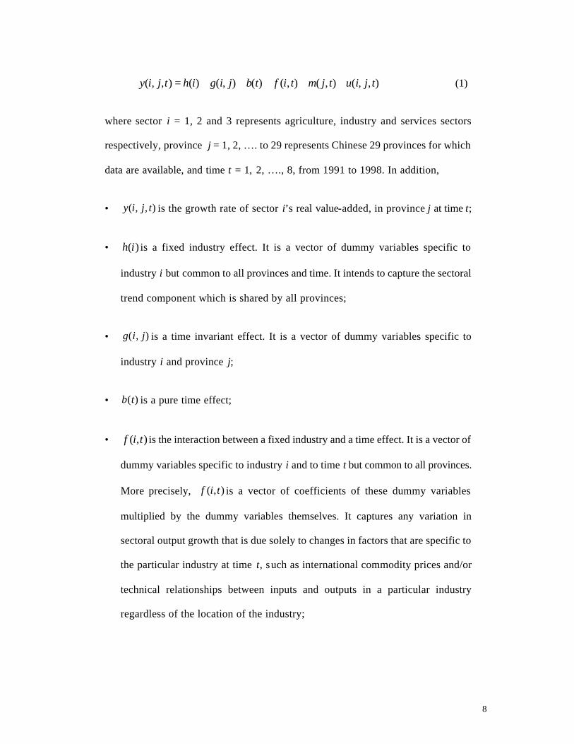
),,(),(),()(),()(),,( tjiutjmtiftbjigihtjiy +++++= (1)

where sector i = 1, 2 and 3 represents agriculture, industry and services sectors

respectively, province j = 1, 2, …. to 29 represents Chinese 29 provinces for which

data are available, and time t = 1, 2, …., 8, from 1991 to 1998. In addition,

• ),,( tjiy is the growth rate of sector i’s real value-added, in province j at time t;

• )(ih is a fixed industry effect. It is a vector of dummy variables specific to

industry i but common to all provinces and time. It intends to capture the sectoral

trend component which is shared by all provinces;

• ),( jig is a time invariant effect. It is a vector of dummy variables specific to

industry i and province j;

• )(tb is a pure time effect;

• ),( tif is the interaction between a fixed industry and a time effect. It is a vector of

dummy variables specific to industry i and to time t but common to all provinces.

More precisely, ),( tif is a vector of coefficients of these dummy variables

multiplied by the dummy variables themselves. It captures any variation in

sectoral output growth that is due solely to changes in factors that are specific to

the particular industry at time t, such as international commodity prices and/or

technical relationships between inputs and outputs in a particular industry

regardless of the location of the industry;

9

• ),( tjm is the interaction between a fixed province and a time effect. It is a vector

of dummy variables (multiplied by their coefficients) for each province j at each

time period t, but is common across industries within each province. It is intended

to represent the effects of province-specific shocks such as changes in monetary or

fiscal policies that lead to different variations in sectoral output in different

provinces;

• ),,( tjiu is an idiosyncratic disturbance to industry i in province j at time t,

assumed to be an independently and identically distributed, normal random

variable with zero mean.

The long run comovements across provinces are captured by the first two terms,

)(ih and ),( jig while the short run components include )(tb , ),( tif and ),( tjm ,

which are common business cycle, sectoral and provincial effects at annual

frequencies. The model may be estimated using a dummy variable method. Direct

estimation of the model in (1) is impossible due to the obvious dummy variab le trap

problem. There are two basic approaches in the literature in dealing with the perfect

collinearity of dummies. One is to choose a province and time period as reference

point and impose such a set of normalizations so that combinations of parameters can

be identified through this set of normalizations, such as in Stockman (1988) and

Costello (1993). It has been shown that there are two shortcomings for this approach

(Marimon and Zilibotti (1998)). First, the results of the variance decomposition are

reference-point dependent. Second, it is difficult to disentangle the covariation of

provincial and sectoral effects since they are correlated and one can only account for

the orthogonal components of each effect.

10

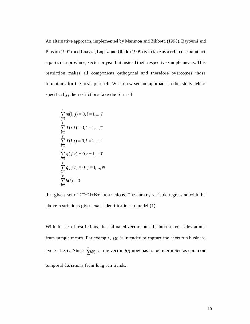
An alternative approach, implemented by Marimon and Zilibotti (1998), Bayoumi and

Prasad (1997) and Loayza, Lopez and Ubide (1999) is to take as a reference point not

a particular province, sector or year but instead their respective sample means. This

restriction makes all components orthogonal and therefore overcomes those

limitations for the first approach. We follow second approach in this study. More

specifically, the restrictions take the form of

∑=

==N

j

Iijim1

,...,1,0),(

∑=

==I

i

Tttif1

,...,1,0),(

∑=

==T

t

Iitif1

,...,1,0),(

∑=

==N

j

Tttjg1

,...,1,0),(

∑=

==T

t

Njtjg1

,...,1,0),(

∑=

=T

t

tb1

0)(

that give a set of 2T+2I+N+1 restrictions. The dummy variable regression with the

above restrictions gives exact identification to model (1).

With this set of restrictions, the estimated vectors must be interpreted as deviations

from sample means. For example, )(tb is intended to capture the short run business

cycle effects. Since ∑=

=T

t

tb1

0)( , the vector )(tb now has to be interpreted as common

temporal deviations from long run trends.

11

3. The Data

To perform the above statistical decomposition, we need the data on growth rates of

sectoral output value-added by province. These data are generally available from

China Statistical Yearbook (CSYB). However, data for 1995 have not been published

and data for 1998 are generally regarded as problematic.5 To estimate provincial

sectoral output value-added growth for 1995 and 1998, we make use of the following

data from CSYB and Almanac of China’s economy 1996: (1) Sectoral value-added at

current price by province in 1994, 1995, 1997 and 1998 (data for 1995 are taken from

Almanac of China’s economy 1996 and data for other years are from CSYB); (2)

Sectoral composition by province in 1994 and 1997; (3) GDP growth rate by

province.

Our procedure for calculating the data on growth of sectoral output value-added by

province in 1995 and 1998 is as follows . With provincial real GDP growth data and

sectoral value-added at current price in 1994 and 1997 available from CSYB, it is

straightforward to calculate the provincial GDP at constant price in 1995 and 1998

(constant at 1994 and 1997 price respectively). The GDP deflator in 1995 and 1998 is

then calculated by dividing the provincial GDP at current price by that at constant

price. The resulting provincial GDP deflator for 1995 and 1998 are used to deflate the

provincial sectoral value-added at current price to get the provincial sectoral value-

added at constant price. The growth rates of sectoral output value-added by province

are then calculated as percentage changes of the provincial sectoral value-added at

5 Recently published provincial GDP data for 1998 suffer from deficiencies that are widely discussed in the Chinese media. To be prudent we use our own estimates and check their consistency with national data (see below detailed estimation procedure and consistency check).

12

constant price in 1995 and 1998 with respect to the provincial sectoral value-added at

current price in 1994 and 1997 respectively .6

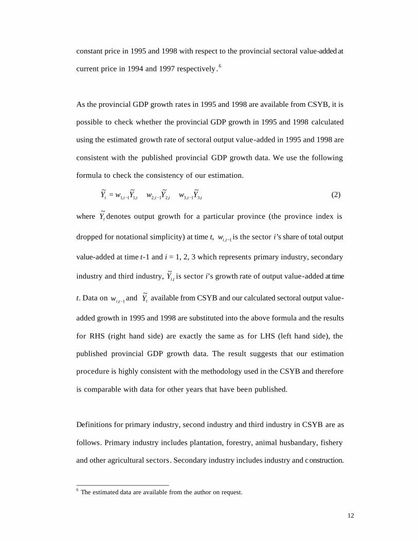
As the provincial GDP growth rates in 1995 and 1998 are available from CSYB, it is

possible to check whether the provincial GDP growth in 1995 and 1998 calculated

using the estimated growth rate of sectoral output value-added in 1995 and 1998 are

consistent with the published provincial GDP growth data. We use the following

formula to check the consistency of our estimation.

ttttttt YwYwYwY ,31,3,21,2,11,1

~~~~−−− ++= (2)

where tY~

denotes output growth for a particular province (the province index is

dropped for notational simplicity) at time t, 1, −tiw is the sector i’s share of total output

value-added at time t-1 and i = 1, 2, 3 which represents primary industry, secondary

industry and third industry, tiY ,

~is sector i’s growth rate of output value-added at time

t. Data on 1, −tiw and tY~

available from CSYB and our calculated sectoral output value-

added growth in 1995 and 1998 are substituted into the above formula and the results

for RHS (right hand side) are exactly the same as for LHS (left hand side), the

published provincial GDP growth data. The result suggests that our estimation

procedure is highly consistent with the methodology used in the CSYB and therefore

is comparable with data for other years that have been published.

Definitions for primary industry, second industry and third industry in CSYB are as

follows. Primary industry includes plantation, forestry, animal husbandary, fishery

and other agricultural sectors. Secondary industry includes industry and construction.

6 The estimated data are available from the author on request.

13

The former is made up of mineral, manufacturing, water supply, electricity, gas, hot

water, steam). Tertiary industry includes those sectors that are not in the category of

primary and second industry, mainly services industry.

4. Statistical Results

The statistical model described in Section 2 is estimated using a dummy variable

regression method for the panel of data described in Section 3. The data are for three

sectors across 29 provinces (See the detailed list in Table 1) from 1991 to 1998. There

are 696 observations in total. The model performs very well. It explains about 90% of

the variations in sectoral value-added growth. The formal statistics of the regression

are R-square = 0.923, adjusted R-square = 0.871, and a highly significant F statistics

with F(302, 394) = 16.518. There is no evidence of serial correlation of the residuals

with Durbin-Watson statistics equal to 2.18.

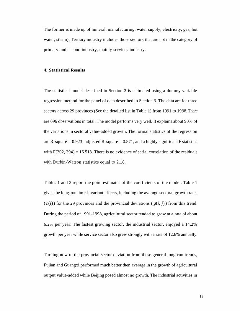
Tables 1 and 2 report the point estimates of the coefficients of the model. Table 1

gives the long-run time-invariant effects, including the average sectoral growth rates

( )(ih ) for the 29 provinces and the provincial deviations ( ),( jig ) from this trend.

During the period of 1991-1998, agricultural sector tended to grow at a rate of about

6.2% per year. The fastest growing sector, the industrial sector, enjoyed a 14.2%

growth per year while service sector also grew strongly with a rate of 12.6% annually.

Turning now to the provincial sector deviation from these general long-run trends,

Fujian and Guangxi performed much better then average in the growth of agricultural

output value-added while Beijing posed almost no growth. The industrial activities in

14

Table 1. Sectoral trends and provincial deviations (%): 1991-1998

Agriculture Industry Service Sectoral trends h(i) 6.155 14.238 12.612 Provincial deviations m(i,j) Beijing -5.318 -4.725 0.413 Tianjin 2.145 -3.538 1.463 Hebei 1.132 1.300 1.651 Shanxi -0.205 -2.788 -3.024 Inner Mongolia 0.907 -2.050 -1.574 Liaoning 1.520 -4.625 -2.174 Jilin 0.795 -2.725 1.101 Heilongjiang -1.018 -6.038 -1.712 Shanghai -2.393 -2.375 1.963 Jiangshu 0.182 2.400 5.763 Zhejiang -1.405 6.538 1.788 Anhui 3.307 3.675 -1.462 Fujian 4.157 8.575 3.701 Jiangxi -1.830 5.250 1.663 Shandong 0.832 2.975 4.363 Henan 0.957 0.663 -0.449 Hubei -1.280 1.975 0.263 Hunan -1.093 0.925 -0.287 Guangdong -0.680 7.513 1.001 Guangxi 4.495 5.913 -0.024 Hainan 3.845 2.463 -1.349 Sichuan -1.955 0.675 -1.237 Guizhou -1.580 -2.813 -1.362 Yunnan -1.205 -1.675 0.151 Shaanxi -0.293 -1.138 -3.974 Gansu -2.230 -2.888 -0.987 Qinghai -2.843 -5.813 -2.012 Ningxia -1.143 -4.738 -3.149 Xinjiang 2.195 -2.913 -0.512

Source: Author's calculations.

the coastal regions, includ ing Zhejiang, Fujian, Guangdong, Jiangshu, Shandong,

Hainan and its neighbouring regions such as Jianxi, Guangxi, Anhui expanded at a

rate that is even higher than the already high average growth (14.2%). China's heavy

industry base, which is the legacy of the centrally planned economy, including the

northeastern provinces of Heilongjiang, Jilin and Liaoning, was not able to exploit the

benefit of China's comparative advantage because of their dominance of state owned

heavy industry enterprises. Service industries in Shanghai and Shandong grew

15

rapidly, at rates much higher than the national average. By contrast, the interior

regions such as Shaanxi, Ningxia, Shanxi and Qinghai lagged substantially behind the

provincial trend average in all sectors.

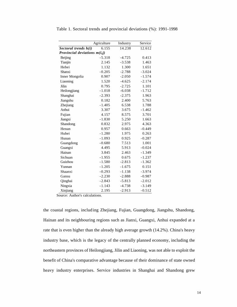
Figure1. China’s Real GDP Growth and Business Cycle: 1991-1998

Source: Author's calculations.

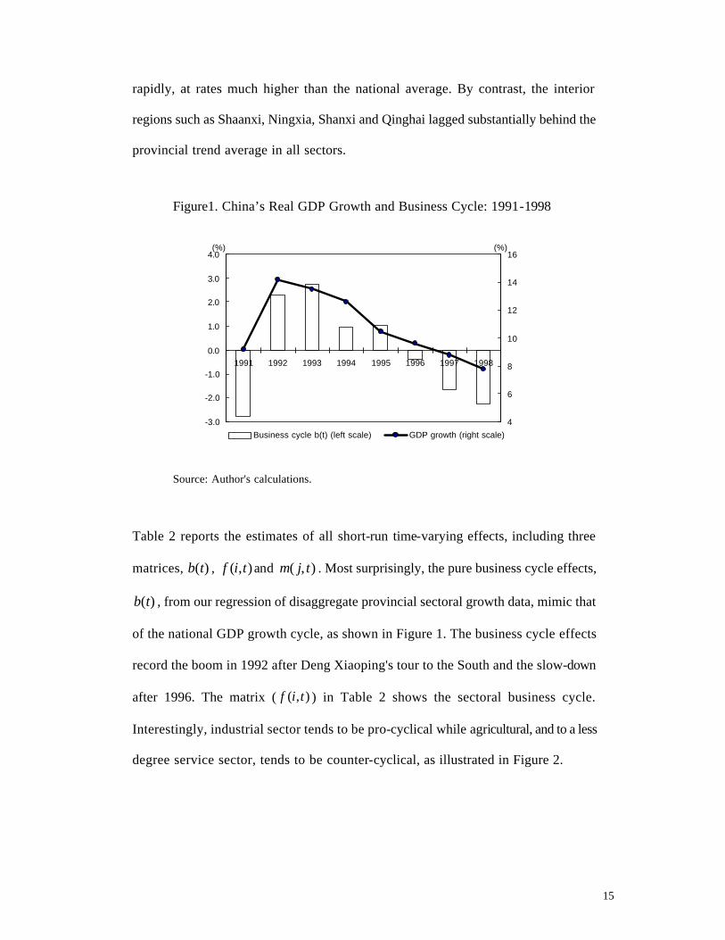
Table 2 reports the estimates of all short-run time-varying effects, including three

matrices, )(tb , ),( tif and ),( tjm . Most surprisingly, the pure business cycle effects,

)(tb , from our regression of disaggregate provincial sectoral growth data, mimic that

of the national GDP growth cycle, as shown in Figure 1. The business cycle effects

record the boom in 1992 after Deng Xiaoping's tour to the South and the slow-down

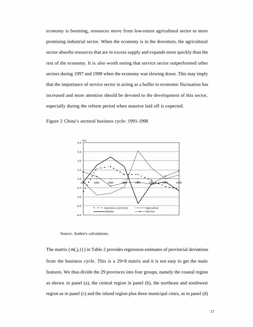
after 1996. The matrix ( ),( tif ) in Table 2 shows the sectoral business cycle.

Interestingly, industrial sector tends to be pro-cyclical while agricultural, and to a less

degree service sector, tends to be counter-cyclical, as illustrated in Figure 2.

-3.0

-2.0

-1.0

0.0

1.0

2.0

3.0

4.0

1991 1992 1993 1994 1995 1996 1997 1998

4

6

8

10

12

14

16

Business cycle b(t) (left scale) GDP growth (right scale)

(%) (%)

16

Table 2 Business cycle and provincial deviations (%): 1991-1998

1991 1992 1993 1994 1995 1996 1997 1998 Business cycle b(t) -2.774 2.304 2.746 0.957 1.046 -0.389 -1.653 -2.237 Sectoral f(i,t) Agriculture -0.757 -3.608 -3.246 -1.854 6.199 2.396 0.019 0.851 Industry -0.757 3.106 4.862 2.723 -5.466 -1.207 -0.633 -2.628 Service 1.514 0.501 -1.616 -0.869 -0.733 -1.188 0.614 1.777

Provincial deviations g(j,t) Beijing 1.449 -0.896 -0.971 1.551 -1.404 -1.836 0.828 1.279 Tianjin -1.418 -4.363 -3.104 -0.116 5.463 1.997 1.561 -0.021 Hebei -0.622 -2.533 0.125 0.814 2.158 -0.274 0.224 0.108 Shanxi -5.322 1.033 -0.475 -1.953 3.092 2.293 -0.743 2.075 Innerm 0.378 -0.767 -2.408 -1.286 -1.908 3.626 0.657 1.708 Liaoning -0.568 -1.346 1.779 -1.199 -0.854 0.747 -0.589 2.029 Jilin -2.551 -0.296 -1.604 2.151 -2.071 3.597 -0.405 1.179 Heilongjiang -0.305 -4.017 -3.758 -0.270 0.542 2.943 3.341 1.525 Shanghai -2.093 -2.504 -3.746 -0.057 3.821 1.622 2.420 0.537 Jiangshu -4.309 8.012 2.038 -1.774 1.204 -1.961 -1.564 -1.646 Zhejiang 3.566 -0.446 1.879 1.634 1.546 -2.586 -2.389 -3.205 Anhui -11.801 1.821 2.446 3.968 4.279 0.047 0.545 -1.305 Fujian 0.595 1.417 4.375 2.064 -1.858 -1.690 -1.559 -3.342 Jiangxi -0.789 1.000 -1.275 2.814 0.658 0.626 0.224 -3.259 Shandong 2.849 3.071 -0.137 0.451 0.296 -2.203 -2.772 -1.555 Henan -1.351 -1.163 -2.771 -0.416 3.029 2.297 0.461 -0.088 Hubei -3.880 -2.325 -0.500 1.655 2.200 0.701 2.199 -0.050 Hunan 0.124 -0.254 -0.229 -1.141 -1.062 1.539 1.170 -0.146 Guangdong 5.061 3.350 1.542 0.530 -0.525 -4.124 -3.126 -2.709 Guangxi 1.878 2.100 5.458 0.147 0.292 -4.174 -3.743 -1.959 Hainan 3.920 11.775 9.767 -0.845 -10.600 -7.899 -4.501 -1.617 Sichuan 0.245 0.333 0.392 -0.653 -1.308 -0.607 0.891 0.708 Guizhou 4.091 -0.888 -1.596 -1.574 -2.729 -0.161 1.170 1.687 Yunnan 1.016 -0.629 -1.137 0.018 0.263 0.264 0.495 -0.288 Shaanxi 3.774 -3.904 0.454 -3.491 -0.846 1.455 0.686 1.870 Gansu -0.093 -1.738 -0.546 -0.024 -2.312 2.755 -0.280 2.237 Qinghai -0.105 -2.617 -2.092 -0.836 0.242 0.710 2.241 2.458 Ningxia -0.051 -3.863 -1.171 -1.482 -1.271 4.230 0.595 3.012 Xinjiang 6.316 0.637 -2.737 -0.682 -0.337 -3.936 1.961 -1.221

Source: Author's calculations.

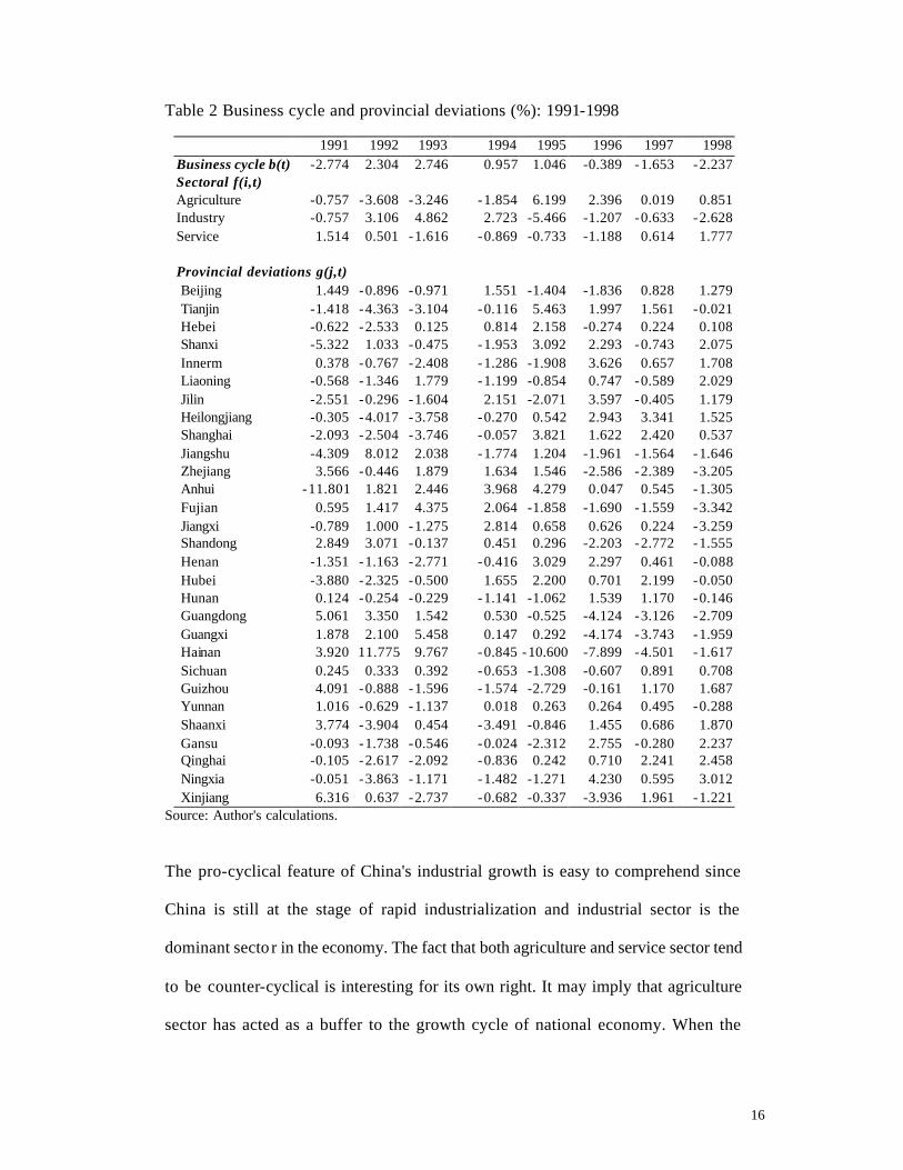
The pro-cyclical feature of China's industrial growth is easy to comprehend since

China is still at the stage of rapid industrialization and industrial sector is the

dominant secto r in the economy. The fact that both agriculture and service sector tend

to be counter-cyclical is interesting for its own right. It may imply that agriculture

sector has acted as a buffer to the growth cycle of national economy. When the

17

economy is booming, resources move from low-return agricultural sector to more

promising industrial sector. When the economy is in the downturn, the agricultural

sector absorbs resources that are in excess supply and expands more quickly than the

rest of the economy. It is also worth noting that service sector outperformed other

sectors during 1997 and 1998 when the economy was slowing down. This may imply

that the importance of service sector in acting as a buffer to economic fluctuation has

increased and more attention should be devoted to the development of this sector,

especially during the reform period when massive laid off is expected.

Figure 2 China’s sectoral business cycle: 1991-1998

Source: Author's calculations.

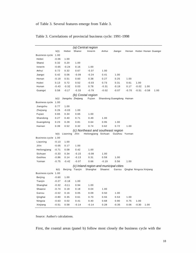
The matrix ( ),( tjm ) in Table 2 provides regression estimates of provincial deviations

from the business cycle. This is a 29×8 matrix and it is not easy to get the main

features. We thus divide the 29 provinces into four groups, namely the coastal region

as shown in panel (a), the central region in panel (b), the northeast and southwest

region as in panel (c) and the inland region plus three municipal cities, as in panel (d)

-8.0

-6.0

-4.0

-2.0

0.0

2.0

4.0

6.0

8.0

1991 1992 1993 1994 1995 1996 1997 1998

Business cycle b(t) AgricultureIndustry Service

(%)

18

of Table 3. Several features emerge from Table 3.

Table 3. Correlations of provincial bus iness cycle: 1991-1998

(a) Central region b(t) Hebei Shanxi Innerm Anhui Jiangxi Henan Hubei Hunan Guangxi

Business cycle 1.00

Hebei -0.06 1.00

Shanxi 0.32 0.20 1.00

Innerm -0.65 -0.24 0.16 1.00

Anhui 0.72 0.32 0.67 -0.37 1.00

Jiangxi 0.42 0.06 -0.09 -0.24 0.41 1.00

Henan -0.19 0.51 0.60 0.38 0.27 0.25 1.00

Hubei 0.13 0.72 0.52 -0.03 0.73 0.31 0.61 1.00

Hunan -0.43 -0.32 0.03 0.78 -0.31 -0.19 0.17 -0.02 1.00

Guangxi 0.58 -0.17 -0.33 -0.79 -0.02 -0.07 -0.70 -0.51 -0.58 1.00

(b) Costal region b(t) Jiangshu Zhejiang Fujian Shandong Guangdong Hainan

Business cycle 1.00 Jiangshu 0.77 1.00 Zhejiang 0.26 -0.03 1.00 Fujian 0.65 0.34 0.65 1.00 Shandong 0.27 0.40 0.71 0.49 1.00 Guangdong 0.23 0.28 0.81 0.64 0.95 1.00 Hainan 0.39 0.52 0.32 0.74 0.62 0.72 1.00

(c) Northeast and southeast region b(t) Liaoning Ji l in Heilongjiang Sichuan Guizhou Yunnan

Business cycle 1.00 Liaoning -0.13 1.00 Ji l in -0.05 0.17 1.00 Heilongjiang -0.71 0.08 0.42 1.00 Sichuan -0.33 0.34 -0.15 -0.08 1.00 Guizhou -0.86 0.14 -0.13 0.31 0.59 1.00 Yunnan -0.75 -0.42 -0.07 0.66 -0.19 0.56 1.00

(c) Inland region and municipal cities b(t) Beij ing Tianjin Shanghai Shaanxi Gansu Qinghai Ningxia Xinjiang

Business cycle 1.00 Beij ing -0.60 1.00 Tianjin -0.27 -0.18 1.00 Shanghai -0.32 -0.11 0.94 1.00 Shaanxi -0.74 0.18 0.18 0.04 1.00 Gansu -0.52 0.16 0.05 0.09 0.50 1.00 Qinghai -0.80 0.35 0.61 0.70 0.55 0.53 1.00 Ningxia -0.63 0.02 0.41 0.40 0.68 0.90 0.75 1.00 Xinjiang -0.51 0.58 -0.14 -0.14 0.28 -0.35 0.06 -0.30 1.00 Source: Author's calculations.

First, the coastal areas (panel b) follow most closely the business cycle with the

19

exception of Hainan, the newly-established province located at the far south of China,

where boom and bust are more pronounced than others. This may reflect the fact that

the coastal regions have been at the center of rapid growth during the reform period.

Second, growth cycle of the central region (panel (a)) also tends to follow the growth

cycle but at a varying degree (first column). This may be interpreted as spillover

effects from the neighboring coastal regions.

Third, other regions, as shown in panels (c) and (d), reveal rather different cyclical

patterns. Interestingly, they tend to be counter-cyclical (first column). When the

overall business cycle is booming, these regions under-performed vis -à-vis the rest of

the economies, and vice versa. Although the pro - and counter-cyclical feature of the

business cycle in regional dimension is itself an interesting subject to explore, it is

beyond the scope of this paper. However, some tentative explanations may be useful.

Labor migration, especially migration from inland, rural areas to coastal regions has

been a significant phenomenon in the last decade. The coastal regions of China, for

various reasons such as special preferential tax treatment for foreign investors, have

been in forefront of economic growth in China. When these regions are booming, the

demand for labor increases, which attracts the influx of rural migrants from other

regions. The influx of migrants has contributed significantly to the already rapid

growth of the coastal regions.

Similar story applies to the flow of capital and skilled workers. Graduate students tend

to find jobs that offer high pay so they tend to choose to work in the coastal regions

and big cities. It is not uncommon that many inland companies have sub-companies or

20

joint venture in the coastal regions with an aim to establish a ‘window’ for contact

with the outside world. The direct investment in coastal regions from inland also helps

to explain the pro-cyclical feature in coastal regions. When the coastal regions are in

economic bust, rural migrants find it difficult to get a job and usually return back to

their hometowns. Direct investment from inland also shrinks. All these have

contributed to the under-performance of the coastal regions.

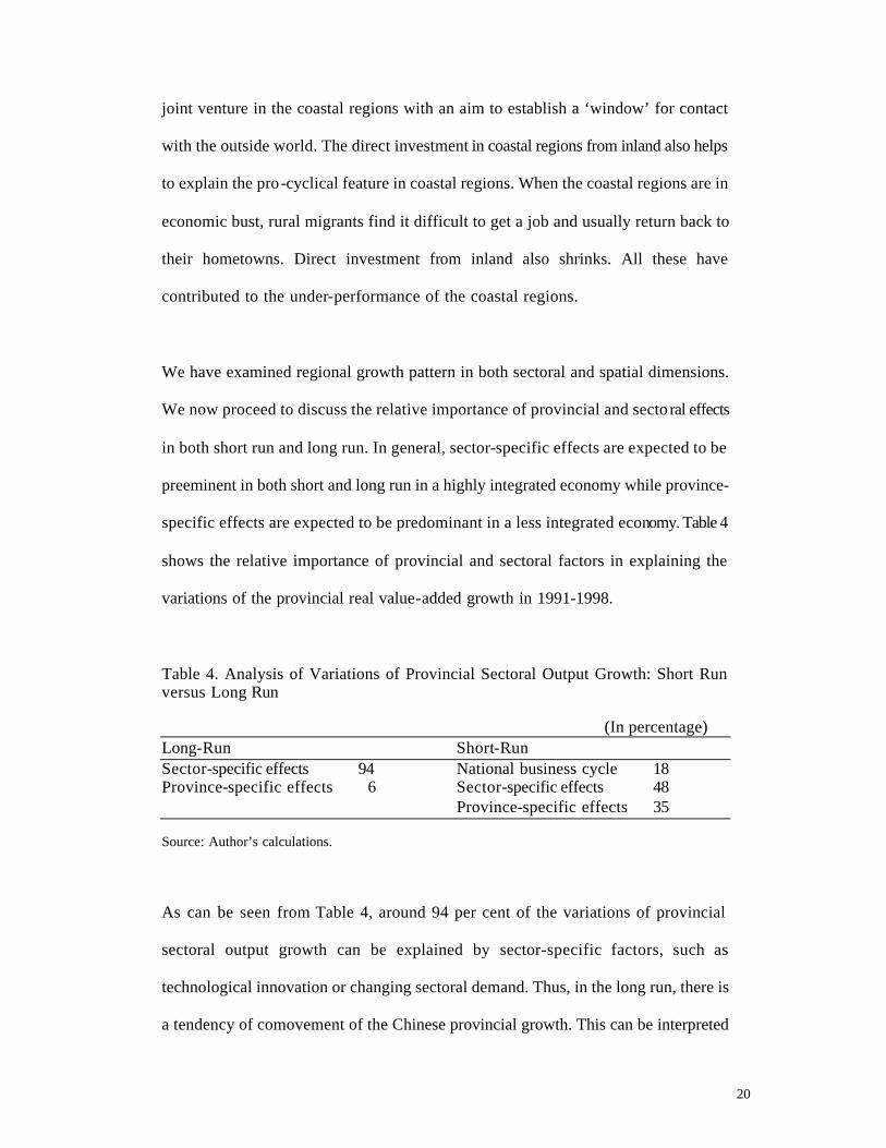
We have examined regional growth pattern in both sectoral and spatial dimensions.

We now proceed to discuss the relative importance of provincial and secto ral effects

in both short run and long run. In general, sector-specific effects are expected to be

preeminent in both short and long run in a highly integrated economy while province-

specific effects are expected to be predominant in a less integrated economy. Table 4

shows the relative importance of provincial and sectoral factors in explaining the

variations of the provincial real value-added growth in 1991-1998.

Table 4. Analysis of Variations of Provincial Sectoral Output Growth: Short Run versus Long Run (In percentage) Long-Run Short-Run Sector-specific effects 94 National business cycle 18 Province-specific effects 6 Sector-specific effects 48 Province-specific effects 35 Source: Author’s calculations.

As can be seen from Table 4, around 94 per cent of the variations of provincial

sectoral output growth can be explained by sector-specific factors, such as

technological innovation or changing sectoral demand. Thus, in the long run, there is

a tendency of comovement of the Chinese provincial growth. This can be interpreted

21

as a sign of increasing integration between Chinese provinces, from a long-run

perspective. On the other hand, province-specific factors still account for one-third of

the variance of real output growth in the short run although sector-specific effects

accounts for 48 percent of the variations, which is consistent with the long-run results.

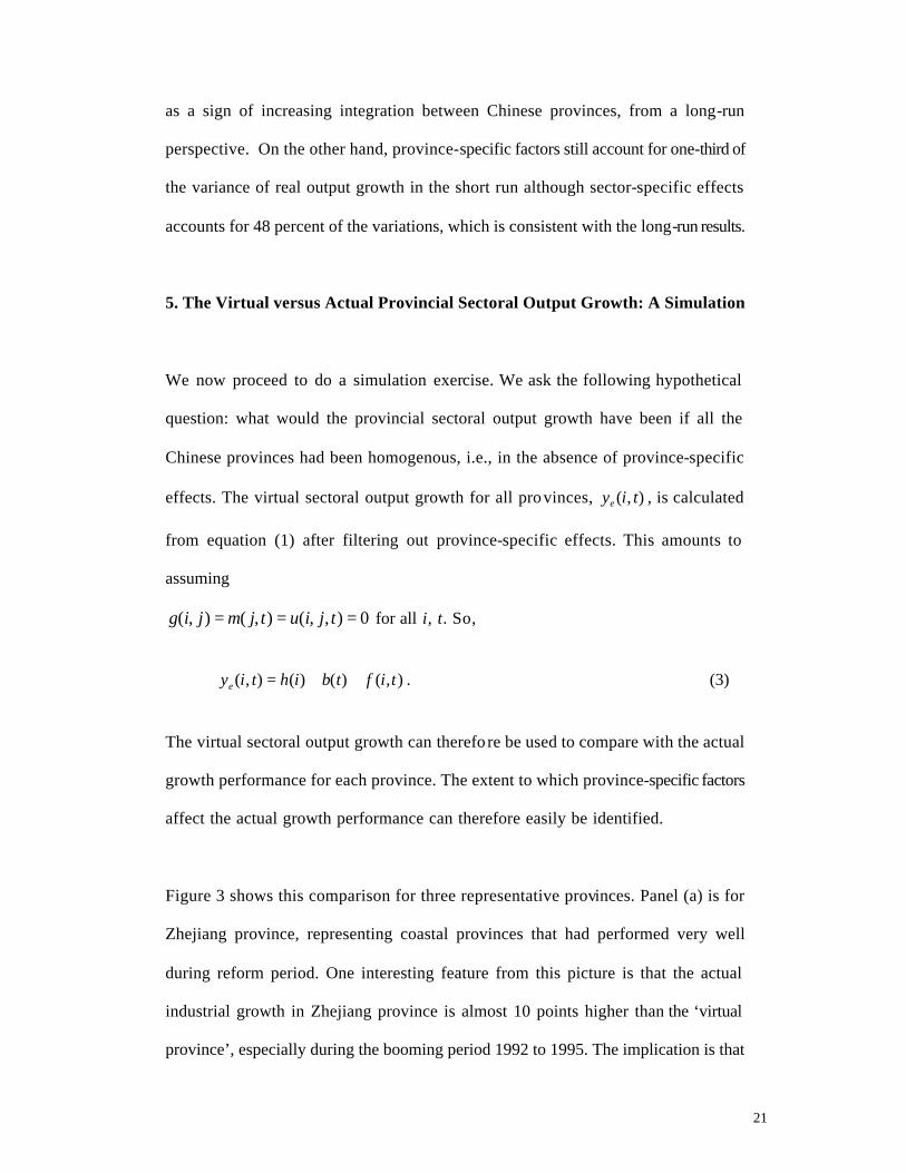
5. The Virtual versus Actual Provincial Sectoral Output Growth: A Simulation

We now proceed to do a simulation exercise. We ask the following hypothetical

question: what would the provincial sectoral output growth have been if all the

Chinese provinces had been homogenous, i.e., in the absence of province-specific

effects. The virtual sectoral output growth for all provinces, ),( tiye , is calculated

from equation (1) after filtering out province-specific effects. This amounts to

assuming

0),,(),(),( === tjiutjmjig for all i, t. So,

),()()(),( tiftbihtiye ++= . (3)

The virtual sectoral output growth can therefore be used to compare with the actual

growth performance for each province. The extent to which province-specific factors

affect the actual growth performance can therefore easily be identified.

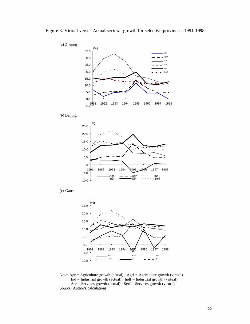
Figure 3 shows this comparison for three representative provinces. Panel (a) is for

Zhejiang province, representing coastal provinces that had performed very well

during reform period. One interesting feature from this picture is that the actual

industrial growth in Zhejiang province is almost 10 points higher than the ‘virtual

province’, especially during the booming period 1992 to 1995. The implication is that

22

Figure 3. Virtual versus Actual sectoral growth for selective provinces: 1991-1998 (a) Zhejing

(b) Beijing (c) Gansu Note: Agr = Agriculture growth (actual) ; Agrf = Agriculture growth (virtual) Ind = Industrial growth (actual) ; Indf = Industrial growth (virtual) Ser = Services growth (actual) ; Serf = Services growth (virtual)

Source: Author's calculations.

-10.0

-5.0

0.0

5.0

10.0

15.0

20.0

25.0

1991 1992 1993 1994 1995 1996 1997 1998

Agr Agrf IndIndf Ser Serf

(%)

-5.0

0.0

5.0

10.0

15.0

20.0

25.0

30.0

35.0

1991 1992 1993 1994 1995 1996 1997 1998

A g r

A g r f

I n d

I n d f

S e r

S e r f

(%)

-10.0

-5.0

0.0

5.0

10.0

15.0

20.0

25.0

1991 1992 1993 1994 1995 1996 1997 1998

A g r A g r f I n d

I n d f S e r S e r f

(%)

23

there are indeed strong province-specific factors underlying Zhejiang’ rapid industrial

growth. In contrast, Beijing’s actual industrial growth is 4.7 percentage points lower

than it could have achieved had its province-specific factors been removed during this

period, as shown in panel (b) of Figure 3.

Other provinces like Liaoning reveal similar pattern. It implies that there were

unfavorable factors not conducive to industrial growth in these provinces. 7 Panel (c)

provides hypothetical and actual sectoral performance for Gansu province,

representing the inland provinces. Their actual industrial performance was not as bad

as one would expect. Again, the counter cyclical feature is prominent in the

comparisons of hypothetical and actual sectoral performance for agriculture and

service sectors.

This simple simulation exercise provides some insights into the degree of Chinese

provincial integration from an alternative perspective. The comparison between

hypothetical and actual provincial sectoral performance reveals distinctive patterns for

Chinese provinces. Province-specific factors are still important factors explaining the

differences in the provincial sectoral growth.

6. Conclusions

Regional economic integration has significant implications not only for the efficient

resource allocation and regional economic development, but also for monetary

policy, as illustrated by the theory of optimal currency area. In this study, we

investigated this important issue using the error-components model. The model

24

enables us to decompose sectoral real value-added growth in each province into

national effects, industry-specific effects and province-specific effects. Provincial

sectoral output growth data for the period of 1991 to 1998 are used.

We found significant comovements in the long run although province-specific

factors still account for one-third of the variance of real output growth in the short

run in the 29 provincial sample. Most strikingly, we are able to trace out the nation’s

business cycle during the 1990s using the disaggregate pooled dataset.

We have also examined regional growth pattern in both sectoral and spatial

dimensions. In the sectoral dimension, we found that industrial sector tends to be

pro-cyclical while agricultural, and to a lesser degree service sector, tends to be

counter-cyclical. The pro-cyclical feature of China's industrial growth is easy to

understand since China is still at the stage of rapid industrialization, and industrial

sector is the dominant sector in the economy. The fact that both agriculture and

service sectors tend to be counter-cyclical may imply that agriculture sector has acted

as a buffer to the growth cycle of national economy. It is also worth noting that

service sector outperformed other sectors during 1997 and 1998 when the economy

was slowing down. This may imply that the importance of service sector in acting as

a buffer to economic fluctuation has increased and more attention should be devoted

to the development of this sector, especially during the reform period when massive

laid off is expected.

In the spatial dimension, we found that: First, the coastal areas follow most closely

7 One potential explanation maybe the dominant feature of state-owned enterprises in these provinces.

25

with the national business cycle. This may reflect the fact that the coastal regions have

been at the center of rapid growth during the reform period. Second, growth cycle of

the central region also tends to follow the national growth cycle but at a varying

degree. This may be interpreted as spillover effects from the neighboring coastal

regions. Third, other regions reveal rather different cyclical patterns. Interestingly,

they tend to be counter-cyclical. Some potential explanations have been offered.

We have also asked the following hypothetical question: what would have been the

provincial sectoral output growth if all the Chinese provinces were homogenous, i.e.,

in the absence of province-specific effects. After filtering out province-specific

effects, we are able to construct hypothetical provincial sectoral growth rates that are

in sharp contrast to the actual regional growth pattern. Province-specific factors are

still important factors explaining differences in the provincial sectoral growth. The

integration of Chinese provinces, although has progressed in a positive way from a

long run perspective, is still far from over.

26

References

Bayoumi, Tamim and Eswar Prasad (1997), ‘Currency Unions, Economic Fluctuations, and Adjustment: Some New Empirical Evidence’, IMF Staff Papers, 44(1): 36–58. State Statistical Bureau, China Statistical Yearb ook (various issues), China Statistical Press. Costello, Donna M. (1993), ‘A Cross-Country, Cross-Industry Comparison of Productivity Growth’, Journal of Political Economy, 101(2): 207–222. Kwan, C. H. (1998), ‘The Theory of Optimal Currency Areas and the Possibility of Forming a Yen Bloc in Asia,’ Journal of Asian Economics, 9(4): 555–580. Loayza, Norman, Humberto Lopez, and Angel Ubide (1999), ‘Sectoral Macroeconomic Interdependencies: Evidence for Latin America, East Asia and Europe’, IMF Working Paper, International Monetary Fund, Washington D.C. Marimon, Ramon and Fabrizio Zilibotti (1998), ‘‘Actual’ Versus ‘Virtual’ Employment in Europe: Is Spain Different?’ European Economic Review, 42: 123–153. McKinnon, Ronald I. (1963), ‘Optimal Currency Areas ’, American Economic Review, 53(4): 717–725. Mody, Ashoka and Fang-Yi Wang. (1997), ‘Explaining Industrial Growth in Coastal China: Economic Reforms … and What Else?’ World Bank Economic Review , 11(2): 293–325. Mundell, Robert A. (1961), ‘A Theory of Optimal Currency Areas’, American Economic Review, 51: 657–665. Naughton, Barry (1999), ‘How Much Can Regional Integration Do to Unify China’s Markets?’, Paper for Conference on Policy Reform in China, Stanford University, November 18-20, 1999. Stockman, Alan C. (1988), ‘Sectoral and National Aggregate Disturbances to Industrial Ouptut in Seven European Countries’, Journal of Monetary Economics, 21: 387–409. World Bank (1992), ‘China: Reform and the Role of the Plan in the 1990s’, World Bank, Washington, D.C. World Bank (1994), ‘China: Internal Market Development and Regulation’, World Bank, Washington, D.C. Young, Alwyn (2000), ‘The Razor’s Edge: Distortions and Incremental Reform in the People’s Republic of China’, NBER Working Paper 7828.