The following presentation of Carl Gauss’sdetermination of the orbit of the asteroidCeres, was commissioned by Lyndon H.LaRouche, Jr., in October 1997, as part of anongoing series of Pedagogical Exercises high-lighting the role of metaphor and paradox increative reason, through study of the greatdiscoveries of science. Intended for individualand classroom study, the weekly install-ments—now “chapters”—were later serial-ized in The New Federalist newspaper. Theyare collected here, in their entirety, for thefirst time, incorporating additions and revi-sions to both text and diagrams.

Through the course of their presentation, itbecame necessary for the authors to reviewmany crucial questions in the history of math-ematics, physics, and astronomy. All of theseissues were subsumed in the primary objective,the discovery of the orbit of Ceres. And,because they were written to challenge a layaudience to master unfamiliar and conceptu-ally dense material at the level of axiomaticassumptions, the installments were often pur-posefully provocative, proceeding by way ofcontradictions and paradoxes.

Nonetheless, the pace of the argumentmoves slowly, building its case by constant ref-

erence to what has gone before. It is, therefore,a mountaintop you need not fear to climb!

We begin, by way of a preface, with thefollowing excerpted comments by LyndonH. LaRouche, Jr. The authors return tothem in the concluding stretto. —KK

* * *

From Euclid through Legendre,geometry depended upon axiomat-

ic assumptions accepted as if they wereself-evident. On more careful inspec-tion, it should be evident, that these

by Jonathan Tennenbaum

and Bruce Director

How Gauss Determined

The Orbit of Ceres

PREFACE

4

assumptions are not necessarily true.Furthermore, the interrelationshipamong those axiomatic assumptions, isleft entirely in obscurity. Most conspicu-ous, even today, generally acceptedclassroom mathematics relies upon theabsurd doctrine, that extension in spaceand time proceeds in perfect continuity,with no possibility of interruption, evenin the extremely small. Indeed, everyeffort to prove that assumption, such asthe notorious tautological hoax concoct-ed by the celebrated Leonhard Euler,

FIGURE 1.1. Positions of unknownplanet (Ceres), observed byGiuseppe Piazzi on Jan. 2, Jan. 22,and Feb. 11, 1801, moving slowlycounter-clockwise against the‘sphere of the fixed stars.’

5

Carl F. Gauss

6

was premised upon a geometry which preassumed perfectcontinuity, axiomatically. Similarly, the assumption thatextension in space and time must be unbounded, was shownto have been arbitrary, and, in fact, false.

Bernhard Riemann’s argument, repeated in the con-cluding sentence of his dissertation “On the HypothesesWhich Underlie Geometry,” is, that, to arrive at a suitabledesign of geometry for physics, we must depart the realmof mathematics, for the realm of experimental physics.This is the key to solving the crucial problems of represen-tation of both living processes, and all processes which, likephysical economy and Classical musical composition, aredefined by the higher processes of the individual humancognitive processes. Moreover, since living processes, andcognitive processes, are efficient modes of existence withinthe universe as a whole, there could be no universal physicswhose fundamental laws were not coherent with that anti-entropic principle central to human cognition. . . .

By definition, any experimentally validated principleof (for example) physics, can be regarded as a dimen-sion of an “n-dimensional” physical-space-time geome-try. This is necessary, since the principle was validatedby measurement; that is to say, it was validated by mea-surement of extension. This includes experimentallygrounded, axiomatic assumptions respecting space andtime. The question posed, is: How do these “n” dimen-sions interrelate, to yield an effect which is characteris-tic of that physical space-time? It was Riemann’sgenius, to recognize in the experimental applicationswhich Carl Gauss had made in applying his approachto bi-quadratic residues, to crucial measurements inastrophysics, geodesy, and geomagnetism, the key tocrucial implications of the approach to a general theoryof curved surfaces rooted in the generalization fromsuch measurements. . . .

What Art Must Learn from EuclidThe crucial distinction between that science and artwhich was developed by Classical Greece, as distinctfrom the work of the Greeks’ Egyptian, anti-Mesopotamia, anti-Canaanite sponsors, is expressed mostclearly by Plato’s notion of ideas. The possibility of mod-ern science depends upon, the relatively perfected formof that Classical Greek notion of ideas, as that notion isdefined by Plato. This is exemplified by Plato’s Socraticmethod of hypothesis, upon which the possibility ofEurope’s development depended absolutely. What ispassed down to modern times as Euclid’s geometry,embodies a crucial kind of demonstration of that princi-ple; Riemann’s accomplishment was, thus, to have cor-rected the errors of Euclid, by the same Socratic methodemployed to produce a geometry which had been, up toRiemann’s time, one of the great works of antiquity. This

has crucial importance for rendering transparent theunderling principle of motivic thorough-composition inClassical polyphony. . . .

The set of definitions, axioms, and postulates deducedfrom implicitly underlying assumptions about space, isexemplary of the most elementary of the literate uses ofthe term hypothesis. Specifically, this is a deductive hypoth-esis, as distinguished from higher forms, including non-linear hypotheses. Once the hypothesis underlying aknown set of propositions is established, we may antici-pate a larger number of propositions than those originallyconsidered, which might also be consistent with thatdeductive hypothesis. The implicitly open-ended collec-tion of theorems which might satisfy that latter require-ment, may be named a theorem-lattice . . . .

The commonly underlying principle of organizationinternal to each such type of deductive lattice, is extension,as that principle is integral to the notion of measurement.This notion of extension, is the notion of a type of exten-sion characteristic of the domain of the relevant choice oftheorem-lattice. All scientific knowledge is premisedupon matters pertaining to a generalized notion of exten-sion. Hence, all rational thought, is intrinsically geomet-rical in character.

In first approximation, all deductively consistent sys-tems may be described in terms of theorem-lattices. How-ever, as crucial features of Riemann’s discovery illustratemost clearly, the essence of human knowledge is change,change of hypothesis, this in the sense in which the prob-lem of ontological paradox is featured in Plato’s Par-menides. In short, the characteristic of human knowledge,and existence, is not expressible in the mode of deductivemathematics, but, rather, must be expressed as change,from one hypothesis, to another. The standard for change,is to proceed from a relatively inferior, to superior hypo-thesis. The action of scientific-revolutionary change, froma relatively inferior, to relatively superior hypothesis, is thecharacteristic of human progress, human knowledge, andof the lawful composition of that universe, whose masterymankind expresses through increases in potential relativepopulation-density of our species.

The process of revolutionary change occurs onlythrough the medium of metaphor, as the relevant princi-ple of contradiction has been stated, above. Just as Euclidwas necessary, that the work of descriptive geometry byGaspard Monge et al., the work of Gauss, and so forth,might make Riemann’s overturning Euclid feasible, so allhuman progress, all human knowledge is premised uponthat form of revolutionary change which appears as theagapic quality of solution to an ontological paradox.

—Lyndon H. LaRouche, Jr.,adapted from “Behind the Notes”Fidelio, Summer 1997 (Vol.VI, No. 2)

January 1, 1801, the first day of a new century. In theearly morning hours of that day, Giuseppe Piazzi,peering through his telescope in Palermo, discovered

an object which appeared as a small dot of light in thedark night sky. (Figure 1.1) He noted its position withrespect to the other stars in the sky. On a subsequentnight, he saw the same small dot of light, but this time itwas in a slightly different position against the familiarbackground of the stars.

He had not seen this object before, nor were there anyrecorded observations of it. Over the next several days,Piazzi watched this new object, carefully noting its changein position from night to night. Using the methodemployed by astronomers since ancient times, he recordedits position as the intersection of two circles on an imagi-nary sphere, with himself at the center. (Figure 1.2a)(Astronomers call this the “celestial sphere”; the circles aresimilar to lines of longitude and latitude on Earth.) One setof circles was thought of as running perpendicular to thecelestial equator, ascending overhead from the observer’shorizon, and then descending. The other set of circles runsparallel to the celestial equator.

To specify any one of these circles, we require an angu-

lar measurement: the position of a longitudinal circle isspecified by the angle (arc) known as the “right ascension,”and that of a circle parallel to the celestial equator, by the“declination.”* (Figure 1.2b). Hence, two angles suffice tospecify the position of any point on the celestial sphere.This, indeed, is how Piazzi communicated his observa-tions to others.

Piazzi was able to record the changing positions of thenew object in a total of 19 observations made over the fol-lowing 42 days. Finally, on February 12, the object disap-peared in the glare of the sun, and could no longer beobserved. During the whole period, the object’s totalmotion made an arc of only 9° on the celestial sphere.

What had Piazzi discovered? Was it a planet, a star, acomet, or something else which didn’t have a name? (Atfirst, Piazzi thought he had discovered a small comet withno tail. Later, he and others speculated it was a planetbetween Mars and Jupiter.) And now that it had disap-peared, what was its trajectory? When and where could it

7

R.A

. =0

hrs.

ecliptic

star

South CelestialPole

North CelestialPole

Earth

equator

R.A. DE

CL.

�

60°N

30°N

30°S

60°S

SouthCelestialPole

22 h

0

2 h

6h4h

NorthCelestial Pole

��

FIGURE 1.2 The celestial sphere. (a) Since ancient times, astronomers have recorded their observations of heavenly bodies as pointson the inside of an imaginary sphere called the celestial sphere, or “sphere of the fixed stars,” with the Earth at its center. Arcs of rightascension and parallels of declination are shown. (b) Locating the position of an object on the celestial sphere by measuring rightascension and declination.

(a) (b)

CHAPTER 1

Introduction

__________

* Figure 1.1 shows the celestial sphere as seen by an observer, with agrid for measuring right ascension and declination shown mappedagainst it.

be seen again? If it were orbiting the sun, how could its tra-jectory be determined from these few observations madefrom the Earth, which itself was moving around the sun?

Had Piazzi observed the object while it was approach-ing the sun, or was it moving away from the sun? Was itmoving away from the Earth or towards it, when theseobservations were made? Since all the observationsappeared only as changes in position against the back-ground of the stars (celestial sphere), what motion didthese changes in position reflect? What would thesechanges in position be, if Piazzi had observed them fromthe sun? Or, a point outside the solar system itself: a“God’s eye view”? (Figure 1.3)

It was six months before Piazzi’s observations werepublished in the leading German-language journal ofastronomy, von Zach’s Monthly Correspondence for the Pro-motion of Knowledge of the Earth and the Heavens, but newsof his discovery had already spread to the leadingastronomers of Europe, who searched the sky in vain forthe object. Unless an accurate determination of the object’strajectory were made, rediscovery would be unpredictable.

There was no direct precedent to draw upon, to solvethis puzzle. The only previous experience that anyonehad had in determining the trajectory of a new object inthe sky, was the 1781 discovery of the planet Uranus byWilliam Herschel. In that case, astronomers were able toobserve the position of Uranus over a considerable time,recording the changes in the position of the planet withrespect to the Earth.

With these observations, the mathematicians simplyasked, “On what curve is this planet traveling, such thatit would produce these particular observations?” If onecurve didn’t produce the desired mathematical result,another was tried.

As Carl F. Gauss described it in the Preface to his 1809book, Theory of the Motion of the Heavenly Bodies Movingabout the Sun in Conic Sections,

As soon as it was ascertained that the motion of the newplanet, discovered in 1781, could not be reconciled withthe parabolic hypothesis, astronomers undertook to adapta circular orbit to it, which is a matter of simple and veryeasy calculation. By a happy accident, the orbit of thisplanet had but a small eccentricity, in consequence ofwhich, the elements resulting from the circular hypothe-sis sufficed, at least for an approximation, on which thedetermination of the elliptic elements could be based.

There was a concurrence of several other very favor-able circumstances. For, the slow motion of the planet,and the very small inclination of the orbit to the plane ofthe ecliptic, not only rendered the calculations much moresimple, and allowed the use of special methods not suitedto other cases; but they removed the apprehension, lest theplanet, lost in the rays of the sun, should subsequentlyelude the search of observers (an apprehension whichsome astronomers might have felt, especially if its lighthad been less brilliant); so that the more accurate determi-nation of the orbit might be safely deferred, until a selec-tion could be made from observations more frequent andmore remote, such seemed best fitted for the end in view.

Linearization in the Small

The false belief that we need a large number of observa-tions, filling out as large an arc as possible, in order todetermine the orbit of a heavenly body, is a typical prod-uct of the Aristotelean assumptions brought into scienceby the British-Venetian school of mathematics—theschool typified by Paolo Sarpi, Isaac Newton, and Leon-hard Euler. Sarpi et al. insisted that, if we examine small-

8

FIGURE 1.3. Artist’srendering of a “God’s eyeview” of the first sixplanets of the solar system.(Note that the correctplanetary sizes, andrelative distances from thesun of “outer planets”Jupiter and Saturn, arenot preserved.)

9

tained, in this case, only if the problem of determiningthe orbit of an unknown planet is treated as a purelymathematical one.

For example, think of three dots on a plane. (Figure1.5) On how many different curves could these dots lie?Now add more dots. The more dots, covering a greaterpart of the curve, the more precise determination of thecurve. A small change of the position of the dots, can

er and smaller portions of any curve in nature, we shallfind that those portions look and behave more and morelike straight line segments—to the point that, for suffi-ciently small intervals, the difference becomes practicallyinsignificant and can be ignored. This idea came to beknown as “linearization in the small.”

In the mid-Fifteenth century, Nicolaus of Cusa hadalready demonstrated conclusively that linearization inthe small had no place in mathematics—if that mathe-matics were to reflect truth. Cusa demonstrated that thecircle represents a fundamentally different species of curvefrom a straight line, and that this species difference doesnot disappear, or even decrease, when we examine verysmall portions of the circle. (Figure 1.4) With respect totheir increasing number of vertices, the polygonsinscribed in and circumscribing the circle become moreand more unlike it.

Extending Cusa’s discovery to astronomy, JohannesKepler discovered that the solar system was orderedaccording to certain harmonic principles. Each small partof the solar system, such as a small interval of a planetaryorbit, reflected that same harmonic principle completely.Kepler’s call for the invention of a mathematical conceptto measure this self-similarity, provoked G.W. Leibniz todevelop the infinitesimal calculus. The entirety of thework of Sarpi, Newton, and Euler, was nothing but afraud, perpetrated by the Venetian-British oligarchyagainst the work of Cusa, Kepler, and Leibniz.

Applying the false mathematics of Sarpi et al. toastronomy, would mean that the physical Universebecame increasingly linear in the small, and that, there-fore, the smaller the arc spanned by the given series ofobservations, the less those observations tell us about theshape of the orbit as a whole. This delusion can be main-

FIGURE 1.4. Nicolaus of Cusa demonstrated, that no matter how many times its sides are multiplied, the polygon can never attainequality with the circle. The polygon and circle are fundamentally different species of figures.

FIGURE 1.5. (a) Here are just a few of the curves that canbe drawn through the same three points. (b) With moreobservation points, we may find that the curve is not asanticipated.

(a)

(b)

mean a great change in the shape of the curve. The fewerthe dots and the closer together they are, the less precise isthe mathematical determination of the curve.

If this false mathematics were imposed on the Uni-verse, determining the orbit of a planet would hardly bepossible, except by curve-fitting or statistical correlationsfrom as extensive a set of observations as possible. But thechanges of observed positions of an object in the nightsky, are not dots on a piece of paper. These changes ofposition are a reflection of physical action, which is self-similar in every interval of that action, in the sense under-stood by Cusa, Kepler, and Leibniz. The heavenly body isnever moving along a straight line, but diverges from astraight line in every interval, no matter how small, in acharacteristic fashion.

In fact, if we focus on the characteristic features of the“non-linearity in the small” of any orbit, then the smallerthe interval of action we investigate in this way, the moreprecise the determination of the orbit as a whole! Thiskey point will become ever clearer as we work throughGauss’ determination of the orbit of Ceres.

It was only an accident that the problem of the deter-mination of the orbit of Uranus could be solved withoutchallenging the falsehood of linearization in the small.But such accidental success of a wrong method, was shat-tered by the problem presented by Piazzi’s discovery. TheUniverse was demonstrating Euler was a fool.

(Years later, Gauss would calculate in one hour, thetrajectory of a comet, which had taken Euler three daysto figure, a labor in which Euler lost the sight of one eye.“I would probably have become blind also,” Gauss said ofEuler, “if I had been willing to keep on calculating in this

manner for three days!”)It was September of 1801, before Piazzi’s observations

reached the 24-year-old Gauss, but Gauss had alreadyanticipated the problem, and ridiculed other mathemati-cians for not considering it, “since it assuredly commend-

10

FIGURE 1.7. Some characteristic properties of the ellipse (a fuller description is presented in the Appendix).

FIGURE 1.6. Generation of the conic sections by cutting acone with a rotating plane. When the plane is parallel tothe base, the section is a circle. As the plane begins to rotate,elliptical sections are generated, until the plane parallel tothe side of the cone generates a parabola. Further rotationgenerates hyperbolas.

Construction of a tangent tothe ellipse: Draw a circlearound focus f, with radiusequal to the constant distance d + d′. The tangentat any point q is the lineobtained by “folding” thecircle such that point q′touches the second focus f′.This construction can be“inverted” to generateellipses and other conicsections as “envelopes” ofstraight lines (see text andFigure 1.9).

Every ellipse has twofoci f, f′, such that thesum of distances d and d′to any point q on thecircumference of theellipse is a constant.

The ellipse as a“contraction” of thecircumscribed circle, inthe direction perpendicularto the major axis. Theratio pq : pq′ remains thesame, no matter where plies on the major axis.

d d′

f f′

q

q′

q

p

d d′

d′

f f′

q

q′

(a) (c)

(b)

11

ed itself to mathematicians by its difficulty and elegance,even if its great utility in practice were not apparent.”Because others assumed this problem was unsolvable,and were deluded by the accidental success of the wrongmethod, they refused to believe that circumstances wouldarise necessitating its solution. Gauss, on the other hand,considered the solution, before the necessity presenteditself, knowing, based on his study of Kepler and Leib-niz, that such a necessity would certainly arise.

Introducing the Conic SectionsBefore embarking on our journey to re-discover themethod by which Gauss determined the orbit of Ceres, wesuggest the reader investigate for himself certain simplecharacteristics of curves that are relevant to the followingchapters. As we shall show later, Kepler discovered that

the planets known to him moved around the sun in orbitsin the shape of ellipses. By Gauss’s time, objects such ascomets had been observed to move in orbits whose shapewas that of other, related curves. All these related curvescan be generated by slicing a cone at different angles, andare therefore called “conic sections.” (Figure 1.6)

The conic sections can be constructed in a variety ofdifferent ways. (SEE Figure 1.7, as well as the Appendix,“The Harmonic Relationships in an Ellipse”) The readercan get a preliminary sense of some of the geometricalproperties of the conic sections, by carrying out the fol-lowing construction.

Take a piece of waxed paper and draw a circle on it.(Figure 1.8) Then put a dot at the center of the circle.Now fold the circumference onto the point at the centerand make a crease. Unfold the paper and make a new fold,bringing another point on the circumference to the point

FIGURE 1.8. Using paperfolding to generate a circle asan envelope of chords.

. . .

FIGURE 1.9. Conic sections generated as envelopes of straight lines, using the“waxed paper folding” method. (a) Ellipse. (b) Hyperbola. (c) Parabola.

(a) (b)

(c)

at the center. Make another crease. Repeat this processaround the entire circumference (approximately 25 times).At the end of this process, you will see a circle envelopedby the creases in the wax paper.

Now take another piece of wax paper and do thesame thing, but this time put the point a little awayfrom the center. At the end of this process, the creaseswill envelop an ellipse, with the dot being one focus.(Figure 1.9a)

Repeat this construction several times, each time mov-ing the point a little farther away from the center of thecircle. Then try it with the point outside the circle; thiswill generate a hyperbola. (Figure 1.9b) Then make thesame construction, using a line and a point, to construct a

parabola. (Figure 1.9c)In this way, you can construct all the conic sections

as envelopes of lines. Now, think of the different curva-tures involved in each conic section, and the relation-ship of that curvature to the position of the dot (focus).

To see this more clearly, do the following. In each ofthe constructions, draw a straight line from the focus tothe curve. (Figure 1.10) How does the length of this linechange, as it rotates around the focus? How is thischange different in each curve?

Over the next several chapters, we will discover howthese geometrical relationships reflect the harmonicordering of the Universe.

—Bruce Director

12

FIGURE 1.10. The length of a line drawn from the focus to the curve changes as it movesaround the curve, except in the case of the circle. In the case of a planetary orbit, thatlength is the distance from the sun to the planet . Note that the circle and ellipse are closedfigures, whereas the parabola and two-part hyperbola are unbounded.

Circle Ellipse Parabola Hyperbola

CHAPTER 2

Clues from Kepler

What did Gauss do, which other astronomersand mathematicians of his time did not, andwhich led those others to make wildly erro-

neous forecasts on the path of the new planet? Perhapswe shall have to consult Gauss’s great teacher, JohannesKepler, to give us some clues to this mystery.

Gauss first of all adopted Kepler’s crucial hypothesis,that the motion of a celestial object is determined solely by itsorbit, according to the intelligible principles Keplerdemonstrated to govern all known motions in the solarsystem. In the Keplerian determination of orbital motion,no information is required concerning mass, velocity, orany other details of the orbiting object itself. Moreover, asGauss demonstrated, and as we shall rediscover for our-

selves, the orbit and the orbital motion in its totality, canbe adduced from nothing more than the internal “curva-ture” of any portion of the orbit, however small.

Think this over carefully. Here, the science of Kepler,Gauss, and Riemann distinguishes itself absolutely fromthat of Galileo, Newton, Laplace, et al. Orbits andchanges of orbit (which in turn are subsumed by higher-order orbits) are ontologically primary. The relation of theKeplerian orbit, as a relatively “timeless” existence, to thearray of successive positions of the orbiting body, is likethat of an hypothesis to its array of theorems. From thisstandpoint, we can say it is the orbit which “moves” theplanet, not the planet which creates the orbit by itsmotion!

13

If we interfere with the motion of an orbiting object,then we are doing work against the orbit as a whole. Theresult is to change the orbit; and this, in turn, causes thechange in the visible motion of the object, which weascribe to our efforts. That, and not the bestial “pushingand pulling” of Sarpian-Newtonian point-mass physics,is the way our Universe works. Any competent astro-naut, in order to successfully pilot a rendezvous in space,must have a sensuous grasp of these matters. Gauss’sentire method rests upon it.

Gauss adopted an additional, secondary hypothesis,likewise derived from Kepler, for which we have beenprepared by Chapter 1: At least to a very high degree ofprecision, the orbit of any object which does not passextremely close to some other body in our solar system(moons are excluded, for example), has the form of asimple conic section (a circle, an ellipse, a parabola, or ahyperbola) with focal point at the center of the sun.Under such conditions, the motion of the celestial objectis entirely determined by a set of five parameters, knownamong astronomers as the “elements of the orbit,”which specify the form and position of the orbit inspace. Once the “elements” of an orbit are specified, andfor as long as the object remains in the specified orbit, itsmotion is entirely determined for all past, present, andfuture times!

Gauss demonstrated how the “elements” of any orbit,and thereby the orbital motion itself in its totality, can beadduced from nothing more than the curvature of any“arbitrarily small” portion of the orbit; and how the lattercan in turn be be adduced—in an eminently practicalway—from the “intervals,” defined by only three good,closely spaced observations of apparent positions as seenfrom the Earth!

The ‘Elements’ of an Orbit

The elements of a Keplerian elliptical orbit consist of thefollowing:

• Two parameters, determining the position of theplane of the object’s orbit relative to the plane of the Earth’sorbit (called the “ecliptic”). (Figure 2.1) Since the sun isthe common focal point of both orbits, the two orbitalplanes intersect in a line, called the “line of nodes.” Therelative position of the two planes is uniquely deter-mined, once we prescribe:

(i) their angle of inclination to each other (i.e., theangle between the planes); and

(ii) the angle made by the line of nodes with somefixed axis in the plane of the Earth’s orbit.

• Two parameters, specifying the shape and overallscale of the object’s Keplerian orbit. (Figure 2.2) It is notnecessary to go into this in detail now, but the chieflyemployed parameters are:

(iii) the relative scale of the orbit, as specified (forexample) by its width when cut perpendicular to itsmajor axis through the focus (i.e., center of the sun);

(iv) a measure of shape known as the “eccentricity,”which we shall examine later, but whose value is 0 for cir-cular orbits, between 0 and 1 for elliptical orbits, exactly 1for parabolic orbits, and greater than 1 for hyperbolicorbits. Instead of the eccentricity, one can also use the peri-helial distance, i.e., the shortest distance from the orbit tothe center of the sun, or its ratio to the width parameter;

• Lastly, we have: (v) one parameter specifying the angle which the

main axis of the object’s orbit within its own orbitalplane, makes with the line of intersection with theEarth’s orbit (“line of nodes”). For this purpose, we can

ecliptic (plane of Earth's orbit)

line of nodes

inclination of orbital plane to ecliptic

�

�

i

maj

or a

xis

�

FIGURE 2.1. A set of three angles is used tospecify the spatial orientation of a givenKeplerian orbit relative to the orbit of theEarth. (1) Angle of inclination i, whichthe plane of the given orbit makes withthe ecliptic plane (the plane of theEarth’s orbit). (2) Angle �, which theorbit’s major axis makes with the “lineof nodes” (the line of intersection ofthe plane of the given orbit and theecliptic plane). (3) Angle �, whichthe line of nodes makes with somefixed axis � in the ecliptic plane(the latter is generally taken to bethe direction of the “vernalequinox” ).

14

take the angle between the major axis of the object’s orbitand the line of nodes. (Figure 2.1)

The entire motion of the orbiting body is determinedby these elements of the orbit alone. If you have masteredKepler’s principles, you can compute the object’s preciseposition at any future or past time. All that you mustknow, in addition to Kepler’s laws and the five parame-ters just described, is a single time when the planet was (orwill be) in some particular locus in the orbit, such as theperihelial position. (Sometimes, astronomers include thetime of last perihelion-crossing among the “elements.”)

Now, let us go back to Fall 1801, as Gauss ponderedover the problem of how to determine the orbit of theunknown object observed by Piazzi, from nothing but ahandful of observations made in the weeks before it dis-appeared in the glare of the morning sun.

The first point to realize, of course, is that the tiny arcof a few degrees, which Piazzi’s object appeared todescribe against the background of the stars, was not thereal path of the object in space. Rather, the positionsrecorded by Piazzi were the result of a rather complicat-ed combination of motions. Indeed, the observed motionof any celestial object, as seen from the Earth, is com-pounded chiefly from the following three processes, ordegrees of action:

1. The rotation of the Earth on its axis (uniform circularrotation, period one day). (Figure 2.3)

2. The motion of the Earth in its known Keplerian orbitaround the sun (non-uniform motion on an ellipse,period one year). (Figure 2.4)

3. The motion of the planet in an unknown Keplerian

orbit (non-uniform motion, period unknown in thecase of an elliptical orbit, or nonexistent in case of aparabolic or hyperbolic orbit). (Figure 2.5)

Thus, when we observe the planet, what we see is akind of blend of all of these motions, mixed or “multi-plied” together in a complex manner. Within any intervalof time, however short, all three degrees of action areoperating together to produce the apparent positions ofthe object. As it turns out, there is no simple way to “sep-arate out” the three degrees of motion from the observa-tions, because (as we shall see) the exact way the threemotions are combined, depends on the parameters of theunknown orbit, which is exactly what we are trying todetermine! So, from a deductive standpoint, we wouldseem to be caught in a hopeless, vicious circle. We shallget back to this point later.

Although the main features of the apparent motionare produced by the “triple product” of two ellipticalmotion and one circular motion, as just mentioned, sev-eral other processes are also operating, which have a com-paratively slight, but nevertheless distinctly measurableeffect on the apparent motions. In particular, for his pre-cise forecast, Gauss had to take into account the followingknown effects:

4. The 25,700-year cycle known as the “precession of theequinoxes,” which reflects a slow shift in the Earth’saxis of rotation over the period of observation. (Figure2.6) The angular change of the Earth’s axis in thecourse of a single year, causes a shift in the apparentpositions of observed objects of the order of tens of sec-onds of arc (depending on their inclination to the celes-tial equator), which is much larger than the margin of

sun (focus)

'parameter'

major axis

(line of apsides) •

B(semi-minor axis)

csun(focus)

f

A (semi-major axis)

(a) Relative scale (b) Eccentricity

FIGURE 2.2. (a) The relative scale of the orbit can be measured by the line perpendicular to the line of apsides, drawn through thefocus (sun). This line is known as the “parameter” of the orbit. (b) The eccentricity is measured as the ratio of the distance f from thefocus to the center of the orbit (point c, the midpoint of the major axis) divided by the semi-major axis A. For the circle, in whichcase the focus and center coincide, f = 0; for the ellipse, 0 < f/A < 1.

ing the time it takes the light to reach him.

7. The apparent positions of stars and planets, as seenfrom the Earth, are also significantly modified by thediffraction of light in the atmosphere, which bends therays from the observed object, and shifts its apparentposition to a greater or lesser degree, depending on itsangle above the horizon. Gauss assumed that Piazzi, asan experienced astronomer, had already made the nec-

15

precision which Gauss required. (In Gauss’s timeastronomers routinely measured the apparent positionsof objects in the sky to an accuracy of one second ofarc, which corresponds to a 1,296,000th part of a fullcircle. Recall the standard angular measure: one fullcircle = 360 degrees; one degree = 60 minutes of arc;one minute of arc = 60 seconds of arc. Gauss is alwaysworking with parts-per-million accuracy, or better.)

5. The “nutation,” which is a smaller periodic shift in theEarth’s axis, superimposed on the 25,700-year preces-sion, and chiefly connected with the orbit of the moon.

6. A slight shift of the apparent direction of a distantstar or planet relative to the “true” one, called “aber-ration,” due to the compound effect of the finitevelocity of light and the velocity of the observer dur-

FIGURE 2.3. Rotation of Earth (daily). FIGURE 2.4. Orbit of Earth (yearly).

pole of theecliptic

ecliptic

celestialequator

to the

'Pole

Star'

FIGURE 2.5. Unknown orbit of “mystery planet” (periodunknown).

FIGURE 2.6. Precession of the equinoxes (period 25,700years).The “precession” appears as a gradual shift in theapparent positions of rising and setting stars on the horizon,as well as a shift in position of the celestial pole. Thisphenomenon arises because Earth’s axis of rotation is notfixed in direction relative to its orbit and the stars, butrotates (precesses) very slowly around an imaginary axiscalled the “pole of the ecliptic,” the direction perpendicularto the ecliptic plane (the plane of the Earth’s orbit).

16

essary corrections for diffraction in the reported obser-vations. Nevertheless, Gauss naturally had to allow fora certain margin of error in Piazzi’s observations, aris-ing from the imprecision of optical instruments, in thedetermination of time, and other causes.

Finally, in addition to the exact times and observedpositions of the object in the sky, Gauss also had to knowthe exact geographical position of Piazzi’s observatory onthe surface of the Earth.

What Did Piazzi See?Let us assume, for the moment, that the complicationsintroduced by effects 4, 5, 6, and 7 above are of a relative-ly technical nature and do not touch upon what Gausscalled “the nerve of my method.” Focus first on obtainingsome insight into the way the three main degrees ofaction 1, 2, and 3 combine to yield the observed positions.

For exploratory purposes, do something like the follow-ing experiment, which requires merely a large room andtables. (Figures 2.7 and 2.8) Set up one object to representthe sun, and arrange three other objects to represent threesuccessive positions of the Earth in its orbit around the sun.This can be done in many variations, but a reasonable firstselection of the “Earth” positions would be to place themon a circle of about two meters(about 6.5 feet) radius aroundthe “sun,” and about 23 cen-timeters (about 9 inches)apart—corresponding, let ussay, to the positions on the Sun-days of three successive weeks.Now arrange another threeobjects at a greater distancefrom the “sun,” for example 5meters (16 feet), and separatedfrom each other by, say 6 and 7centimeters. These positionsneed not be exactly on a circle,but only very roughly so. Theyrepresent hypothetical positionsof Piazzi’s object on the samethree successive Sundays ofobservation.

For the purpose of the sight-ings we now wish to make, thebest choice of “celestial objects”is to use small, bright-coloredspheres or beads of diameter 1cm or less, mounted at the endof thin wooden sticks which arefixed to wooden disks or otherobjects, the latter serving as

bases placed on the table, as shown in the photograph inFigure 2.7.

Now, sight from each of the Earth positions to the cor-responding hypothetical positions of Piazzi’s object, andbeyond these to a blackboard or posters hung from anopposing wall. Imagine that wall to represent part of thecelestial sphere, or “sphere of fixed stars.” Mark the posi-tions on the wall which lie on the lines of sight betweenthe three pairs of positions of the Earth and Piazzi’sobject. Those three marks on the wall, represent the“data” of three of Piazzi’s observations, in terms of theobject’s apparent position relative to the background ofthe fixed stars, assuming the observations were made onsuccessive Sundays. Experimenting with different relativepositions of the two in their orbits, we can see how theobservational phenomenon of apparent retrograde motionand “looping” can come about (in fact, Piazzi observed aretrograde motion). (Figure 2.9) Experiment also withdifferent arrangements of the spheres representing Piazzi’s object, as might correspond to different orbits.

From this kind of exploration, we are struck by anenormous apparent ambiguity in the observations. WhatPiazzi saw in his telescope was only a very faint point oflight, hardly distinguishable from a distant star except byits motion with respect to the fixed stars from day to day.

FIGURE 2.7. Author Bruce Director demonstrates Piazzi’s sightings. The models on the table inthe foreground represent the three different positions of the Earth. The models on the table infront of the board represent the corresponding positions of Ceres. Marks 1, 2, and 3 on the boardrepresent the sightings of Ceres, as seen from the corresponding positions of the Earth.

EIR

NS

/Mic

hael

Mic

ale

17

On the face of things, there would seem to be no way toknow exactly how far away the object might be, nor inwhat exact direction it might be moving in space. Indeed,all we really have are three straight lines-of-sight, run-ning from each of the three positions of the Earth to thecorresponding marks on the wall. For all we know, eachof the three positions of Piazzi’s object might be locatedanywhere along the corresponding line-of-sight! We doknow the time intervals between the positions we arelooking at (in this case a period of one week), but howcan that help us? Those times, in and of themselves, do

not even tell us how fast the object is really moving, sinceit might be closer or farther away, and moving more orless toward us or away from us.

Try as we will, there seems to be no way to determinethe positions in space from the observations in a deduc-tive fashion. But haven’t we forgotten what Keplertaught us, about the primacy of the orbit, over themotions and positions?

Gauss didn’t forget, and we shall discover his solutionin the coming chapters.

—Jonathan Tennenbaum

1

23

12.35 in.

Earth

Earth orbit

wall('fixedstars')

3Piazzi’s object

1

3

22

sun

9 in.

orbit of Piazzi’s object16 ft.

6 ft.

lines of sight

FIGURE 2.8. Paradoxes of apparent motion. The apparent motion of Ceres as seen from the Earth (here indicated by the

successive positions 1,2,3 on the wall at the right) is very different from the actualmotion of Ceres in its orbit. In the case illustrated here, the order of points 1,2,3 on the

wall is reversed relative to Ceres’ actual positions; thus, Ceres will appear from Earth to bemoving backwards! The bizarre appearance of retrograde motion and “looping” is due to the

differential in motion of Earth and Ceres, combined with their relative configuration in space,Earth’s orbital motion being faster than that of Ceres (see Figure 2.9). In reality, the apparent

motion is further complicated by the circumstance that the two bodies are orbiting in different planes.

FIGURE 2.9. Star charts show apparent retrograde motion for the asteroids (a) Ceres, and (b) Pallas, during 1998.

(a)(b)

18

In investigations such as we are now pursuing, it shouldnot be so much asked “what has occurred,” as “what hasoccurred that has never occurred before.”

—C. Auguste Dupin, in Edgar Allan Poe’s

“The Murders in the Rue Morgue”

With Dupin’s words in mind, let us return to thedilemma in which we had entangled ourselvesin our discussion in the previous chapter. That

dilemma was connected to the fact, that what Piazziobserved as the motion of the unknown object against thefixed stars, was neither the object’s actual path in space,nor even a simple projection of that path onto the celestialsphere of the observer, but rather, the result of the motionof the object and the motion of the Earth, mixed together.

Thanks to the efforts of Kepler and his followers, thedetermination of the orbit of the Earth, subsuming itsdistance and position relative to the sun on any given dayof the year, was quite precisely known by Gauss’s time.Accordingly, we can formulate the challenge posed byPiazzi’s observations in the following way: We candetermine a precise set of positions in space from which

Piazzi’s observations were made, taking into account theEarth’s own motion. From each of the positions ofPalermo, where Piazzi’s observatory was located, draw astraight line-of-sight in the direction in which Piazzi sawthe object at that moment. All we can say with certaintyabout the actual positions of the unknown object at thegiven times, is that each position lies somewhere along thecorresponding straight line. What shall we do?

In the face of such an apparent degree of ambiguity,any attempt to “curve fit” fails. For, there are no well-defined positions on which to “fit” an orbit! But, don’twe know something more, which could help us? After all,Kepler taught that the geometrical forms of the orbits are(to within a very high degree of precision, at least) planeconic sections, having a common focus at the center of thesun. Kepler also provided a crucial, additional set of con-straints (to be examined in Chapter 7), which determinethe precise motion in any given orbit, once the “elements”of the orbit discussed last chapter have been determined.

Now, unfortunately, Piazzi’s observations don’t eventell us what plane the orbit of Piazzi’s object lies in. Howdo we find the right one?

Take an arbitrary plane through the sun. The lines-of-sight of Piazzi’s observations will intersect that plane inas many points, each of which is a candidate for the posi-tion of the object at the given time. Next, try to constructa conic section, with a focus at the sun, which goesthrough those points or at least fits them as closely as pos-sible. (Alas! We are back to curve-fitting!) (Figure 3.1)

Finally—and this is the substantial new feature—check whether the time intervals defined by a Keplerianmotion along the hypothesized conic section between thegiven points, agree with the actual time intervals ofPiazzi’s observations. If they don’t fit, which will be near-ly always the case, then we reject the orbit. For example,if the intersection-points are very far away from the sun,then Kepler’s constraints would imply a very slowmotion in the corresponding orbit; outside a certain dis-tance, the corresponding time-intervals would becomelarger than the times between Piazzi’s actual observa-tions. Conversely, if the points are very close to the sun,the motion would be too fast to agree with Piazzi’s times.

The consideration of time-intervals thus helps to limitthe range of trial-and-error search somewhat, but thedomain of apparent possibilities still remains monstrouslylarge. With the unique exception of Gauss, astronomers

CHAPTER 3

Method—Not Trial-and-Error

E1

E3

E2

O

P3

P2P1

FIGURE 3.1. Piazzi’s observations define three “lines ofsight” from three Earth positions E1 ,E2 ,E3 , but do not tellus where the planet lies on any of those lines. We do knowthat the positions lie on some plane through the sun.

felt themselves forced to make ad hoc assumptions andguesses, in order to radically reduce the range of possibili-ties, and thereby reduce the trial-and-error procedures toa minimum.

For example, the astronomer Wilhelm Olbers andothers decided to start with the working assumption thatthe sought-for orbit was very nearly circular, in whichcase the motion becomes particularly simple. Kepler’sthird constraint (usually referred to as his “Third Law”)determines a specific rate of uniform motion along thecircle, as soon as the radius of the circular orbit isknown. According to that third constraint, the square ofperiodic time in any closed orbit—i.e., a circular or anelliptical one—as measured in years, is equal to the cubeof the orbit’s major axis, as measured in units of themajor axis of the Earth’s orbit. Next, Olbers took two ofPiazzi’s observations, and calculated the radius which a

circular orbit would have to have, in order to fit thosetwo observations.

It is easy to see how to do that in principle: The twoobservations define two lines of sight, each originatingfrom the position of the Earth at the moment of observa-tion. Imagine a sphere of variable radius r, centered at thesun. (Figure 3.2) For each choice of r, that sphere willintersect the lines-of-sight in two points, P and Q.Assuming the planet were actually moving on a circularorbit of radius r, the points P and Q would be the corre-sponding positions at the times of the two observations,and the orbit would be the great circle on the sphere pass-ing through those two points. On the other hand,Kepler’s constraints tell us exactly how large is the arcwhich any planet would traverse, during the time inter-val between the two observations, if its orbit were a circleof radius r. Now compare the arc determined from

19

It seems somewhat strange that thegeneral problem—to determine the

orbit of a heavenly body, without anyhypothetical assumption, from observa-tions not embracing a great period of time,and not allowing a selection with a viewto the application of special methods—was almost wholly neglected up to thebeginning of the present century; or, atleast, not treated by any one in a man-ner worthy of its importance; since itassuredly commended itself to mathe-maticians by its difficulty and elegance,even if its great utility in practice werenot apparent. An opinion had univer-sally prevailed that a complete determi-nation from observations embracing ashort interval of time was impossible,—an ill-founded opinion,—for it is nowclearly shown that the orbit of a heav-enly body may be determined quitenearly from good observations embrac-ing only a few days; and this withoutany hypothetical assumption.

Some ideas occurred to me in themonth of September of the year 1801,[as I was] engaged at that time on avery different subject, which seemedto point to the solution of the greatproblem of which I have spoken.

Under such circumstances we notinfrequently, for fear of being toomuch led away by an attractive inves-tigation, suffer the associations ofideas, which, more attentively consid-ered, might have proved most fruitfulin results, to be lost from neglect. Andthe same fate might have befallenthese conceptions, had they not happi-ly occurred at the most propitiousmoment for their preservation andencouragement that could have beenselected. For just about this time thereport of the new planet, discoveredon the first day of January of that yearwith the telescope at Palermo, was thesubject of universal conversation; andsoon afterwards the observations madeby that distinguished astronomerPiazzi, from the above date to theeleventh of February were published.

Nowhere in the annals of astrono-my do we meet with so great anopportunity, and a greater one couldhardly be imagined, for showing moststrikingly, the value of this problem,than in this crisis and urgent necessity,when all hope of discovering in theheavens this planetary atom, amonginnumerable small stars after the lapse

of nearly a year, rested solely upon asufficiently approximate knowledge ofits orbit to be based upon these veryfew observations. Could I ever havefound a more seasonable opportunityto test the practical value of my con-ceptions, than now in employing themfor the determination of the orbit ofthe planet Ceres, which during theseforty-one days had described a geocen-tric arc of only three degrees, and afterthe lapse of a year must be looked forin a region of the heavens very remotefrom that in which it was last seen?

The first application of the methodwas made in the month of October1801, and the first clear night (Decem-ber 7, 1801), when the planet wassought for as directed by the numbersdeduced from it, restored the fugitiveto observation. Three other new plan-ets subsequently discovered, furnishednew opportunities for examining andverifying the efficiency and generalityof the method. [emphasis in original]

Excerpted from the Preface to the Eng-lish edition of Gauss’s “Theory of theMotion of the Heavenly Bodies Movingabout the Sun in Conic Sections.”

C.F. Gauss: ‘To determine the orbit of a heavenly body, without any hypothetical assumption’

Kepler’s constraint, with the actual arc between P and Q,as the length of radius r varies, and locate the value orvalues of r, for which the two become coincident. Thatdetermination can easily be translated into a mathemati-cal equation whose numerical solution is not difficult towork out. Having found a circular orbit fitting twoobservations in that way, Olbers then used the compari-son with other observations to correct the original orbit.

Toward the end of 1801 astronomers all over Europebegan to search for the object Piazzi had seen in January-February, based on approximations such as Olbers’. Thesearch was in vain! In December of that year, Gauss pub-lished his hypothesis for the orbit of Ceres, based on hisown, entirely new method of calculation. According tocalculations based on Gauss’s elements, the object wouldbe located more than 6° to the south of the positions fore-cast by Olbers, an enormous angle in astronomical terms.Shortly thereafter, the object was found very close to theposition predicted by Gauss.

Characteristically, Gauss’s method used no trial-and-error at all. Without making any assumptions on the par-ticular form of the orbit, and using only three well-chosen observations, Gauss was able to construct a goodfirst approximation to the orbit immediately, and thenperfect it without further observations to a high precision,making possible the rediscovery of Piazzi’s object.

To accomplish this, Gauss treated the set of observa-tions (including the times as well as the apparent posi-tions) as being the equivalent of a set of harmonic intervals.Even though the observations are, as it were, jumbled upby the effects of projection along lines-of-sight andmotion of the Earth, we must start from the standpointthat the underlying curvature, determining an entireorbit from any arbitrarily small segment, is somehow

20

lawfully expressed in such an array of intervals. To deter-mine the orbit of Piazzi’s object, we must be able to iden-tify the specific, tell-tale characteristics which reveal thewhole orbit from, so to speak, “between the intervals” ofthe observations, and distinguish it from all other orbits.This requires that we conceptualize the higher curvatureunderlying the entire manifold of Keplerian orbits, takenas a whole. Actually, the higher curvature required, can-not be adequately expressed by the sorts of mathematicalfunctions that existed prior to Gauss’s work.

We can shed some light on these matters, by the fol-lowing elementary experimental-geometrical investiga-tion. Using the familiar nails-and-thread method, con-

FIGURE 3.3. Constructing an ellipse in the shape of the orbitof Mars.

sunP

Q

r

r′

P′

Q′

E1

E2

CC′

FIGURE 3.2. Method to determine the orbit of Ceres,on the assumption that the orbit is circular. Twosightings of Ceres define two lines of sight comingfrom the Earth positions E1, E2 (the Earth’s positionsat the moments of observation). A sphere around thesun, of radius r, intersects the lines of sight in twopoints P,Q, which lie on a unique great circle C onthat sphere. A sphere of some different radius r′ woulddefine a different set of points P′, Q′ and a differenthypothetical orbit C′. Determine the unique value ofr, for which the size of the arc PQ agrees with the rateof motion a planet would really have, if it weremoving according to Kepler’s laws on the circularorbit C over the time interval between the givenobservations.

21

struct an ellipse having the shape of the Mars orbit, as fol-lows. (Figure 3.3) Hammer two nails into a flat boardcovered with white paper, at a distance of 5.6 cm fromeach other. Take a piece of string 60 cm long and tie eachend to one of the nails—or alternatively, make a loop ofstring of length 60 + 5.6 = 65.6 cm, and loop it aroundboth nails. Pulling the loop tight with the tip of a pencil asshown, trace an ellipse. The positions of the two nails rep-resent the foci. The resulting curve will be a scaled-downreplica of Mars’ orbit, with the sun at one of the foci.

Observe that the circumference generated is hardlydistinguishable, by the naked eye, from a circle. Indeed,mark the midpoint of the ellipse (which will be the pointmidway between the foci), and compare the distancesfrom various points on the circumference, to the center.You will find a maximum discrepancy of only about onemillimeter (more precisely, 1.3 mm), between the maxi-mum distance (the distance between the points on the cir-cumference at the two ends of the major axis connectingthe two foci) and the minimum distance (between theendpoints of the minor axis drawn perpendicular to themajor axis at its mid-point). Thus, this ellipse’s deviationfrom a perfect circle is only on the order of four parts inone thousand. How was Kepler able to detect anddemonstrate the non-circular shape of the orbit of Mars,given such a minute deviation, and how could he correct-

ly ascertain the precise nature of the non-circular form,on the basis of the technology available at his time?

Observe in Figure 3.4a, that the distances to the sun(the marked focus) change very substantially, as we movealong the ellipse.

Now, choose two points P1 and P2 anywhere along thecircumference of the ellipse, two centimeters apart. Theinterval between them would correspond to successivepositions of Mars at times about seven days apart (actual-ly, up to about 10 percent more or less than that, depend-ing on exactly where P1 and P2 lie, relative to the perihe-lion [closest] and aphelion [farthest] positions). Draw radi-al lines from each of P1, P2 to the sun, and label the corre-sponding lengths r1, r2.

Consider what is contained in the curvilinear triangleformed by those two radial line segments and the smallarc of Mars’ trajectory, from P1 to P2. Compare that arcwith that of analogous arcs at other positions on the orbit,and consider the following propositions: Apart from thesymmetrical positions relative to the two axes of theellipse, no two such arcs are exactly superimposable in any oftheir parts. Were we to change the parameters of theellipse—for example, by changing the distance betweenthe foci, by any amount, however small—then none ofthe arcs on the new ellipse, no matter how small, wouldbe superimposable with any of those on the first, in any of

sun

P6

P5

P4

P3

P2

P1

r6r5

r4

r3

r2

r1

(focus)

FIGURE 3.4. (a) The positions of Mars in its orbit around thesun at equal time intervals of approximately 30 days. Notethat the orbital arcs are longer when Mars is closer to the sun(faster motion), shorter when Mars is farther away (slowermotion), in such a way that the areas of the correspondingorbital sectors are equal (Kepler’s “Area Law”). (b) In aclose-up of Mars’ orbit, note the small areas separating thechords and the orbital arcs, and reflecting the curvature ofthe orbit in the given interval. These areas change in size andshape from one part of the orbit to the next, reflecting aconstantly changing curvature.

P2

P1

r6 r5r4

r3

r2

r1

P3

P4

P5

P6(b)(a)

Any successful solution of the problem posed toGauss must pivot on conceptualizing the char-acteristic curvature of Keplerian orbits “in the

small.” Before turning to Kepler’s own investigationson this subject, it may be helpful to take a brief look atthe closely related case of families of catenaries on thesurface of the Earth—these being more easily accessibleto direct experimentation, than the planetary orbitsthemselves.

Catenaries, Monads, and A First Glimpse at Modular FunctionsWhen a flexible chain is suspended from two points, andpermitted to assume its natural form under the action of itsown weight, then, the portion of the chain between thetwo points forms a characteristic species of curve, knownas a catenary. The ideal catenary is generated by a chainconsisting of very small, but strong links made of a rigidmaterial, and having very little friction; such a chain ispractically inelastic (i.e., does not stretch), while at the sametime being nearly perfectly flexible, down to the lower lim-it defined by the diameter of the individual links.

Interestingly, the form of the catenary depends only onthe position of the points of suspension and the length ofthe chain between those points, but not on its mass orweight.

With the help of a suitable, fine-link chain, suspendedparallel to, and not far from, a vertical wall or board (so

that the chain’s form can easily be seen and traced, asdesired), carry out the following investigations.

(For some of these experiments, it is most convenient touse two nails or long pins, temporarily fixed into the wallor board, as suspension-points; the nails or pins should berelatively thin, and with narrow heads, so that the links ofthe chain can easily slip over them, in order to be able tovary the length of the suspended portion. In some experi-ments it is better to fix only one suspension-point with anail, and to hold the other end in your hand.)

Start by fixing any two suspension-points and an arbi-trary chain-length. (Figure 4.1) Observe the way theshape of each part of the catenary, so formed, depends onall the other parts. Thus, if we try to modify any portionof the catenary, by pushing it sideways or upwards with

22

their parts! Thus, each arc is uniquely characteristic ofthe ellipse of which it is a part. The same is true amongall species of Keplerian orbits.

Consider what means might be devised to reconstructthe whole orbit from any one such arc. For example, bywhat means might one determine, from a small portionof a planetary trajectory, whether it belongs to a parabol-ic, hyperbolic, or elliptical orbit?

Now, compare the orbital arc between P1 and P2 withthe straight line joining P1 and P2. (Figure 3.4b) Togeth-er they bound a tiny, virtually infinitesimal area. Evident-ly, the unique characteristic of the particular elliptical

orbit must be reflected somehow in the specific manner inwhich that arc differs from the line, as reflected in that“infinitesimal” area.

Finally, add a third point, P3, and consider the curvi-linear triangles corresponding to each of the three pairs(P1, P2), (P2, P3), and (P1, P3), together with the corre-sponding rectilinear triangles and “infinitesimal” areaswhich compose them. The harmonic mutual relationsamong these and the corresponding time intervals, lie atthe heart of Gauss’s method, which is exactly the oppositeof “linearity in the small.”

—JT

CHAPTER 4

Families of Catenaries(An Interlude Considering Some Unexpected Facts About ‘Curvature’)

A B

FIGURE 4.1 A catenary is formed by suspending a chainbetween points A and B.

23

FIGURE 4.3. Varying the endpoint position of a fixed lengthof chain generates a second family of catenaries.

ABL

B

BB

B

B

B

the tip of a finger, we see that the entire curve is affected,at least slightly, over its entire length. This behavior ofthe catenary reflects Leibniz’s principle of least action,whereby the entire Universe as a whole, including itsmost remote parts, reacts to any event anywhere in theUniverse. There is no “isolated” point-to-point action inthe way the Newtonians claim.

Note that the curvature of each individual catenarychanges constantly along its length, as we go from itslowest point to its highest point.

Next, generate a family of catenaries, by keeping thesuspension-points fixed, but varying the length of thechain between those points. (Figure 4.2) Observe thechanges in the form and curvature, and the changes inthe angles, which the chain makes to the horizontal at thepoints of suspension, as a function of the suspendedlength.

Generate a second family of catenaries, by keeping thechain length and one of the suspension-points fixed, whilevarying the other point. (Figure 4.3) If A is the first sus-pension-point, and L is the length of the suspended chain,then the second suspension-point B (preferably held byhand) can be located anywhere within the circle of radiusL around A. For B on the circumference of the circle, thecatenary degenerates into a straight line. (Or rather, some-thing close to a straight line, since the latter would requirea physically impossible, “infinite tension” to overcome thegravitational effect.) Observe the changes of form, as Bmoves around A in a circle of radius less than L. Also,observe the change in the angles, which the catenarymakes to the horizontal at each of the endpoints, as afunction of the position of B. Finally, observe the changesin the tension, which the chain exerts at the endpoint B,held by hand, as its position is changed.

Examine this second family of catenaries for the case,where the suspended length is extremely short. Combin-ing the variation of the endpoint with variation of length

A B

C

D

S

A B

C

D

S

A B

(a)

(b)

FIGURE 4.2. Varying the lengths of the chain generates afamily of catenaries of varying curvatures.

FIGURE 4.4. Release catenary AB to points C,D. Every arcof a catenary, is itself a catenary!

24

whole. In consequence of this, secondly, when we lookat different parts of a given catenary, we are in a senselooking at different local expressions on the same globalentity. Although various, small portions of the cate-nary have different curvatures in the sense of visualgeometry, in a deeper sense they all share a common“higher curvature,” characteristic of the catenary ofwhich they are parts. Finally, there must be a stillhigher mode of curvature, which defines the commoncharacteristic of the entire family of catenaries. Thatlatter entity would be congruent with Gauss’s conceptof a modular function for the species of catenaries, as aspecial case of his hypergeometric function; the lattersubsuming the catenaries together with the analogous,crucial features of the Keplerian planetary orbits. (Inthe Earth-bound case of elementary catenaries, thedistinction among different catenaries is, to a veryhigh degree of approximation, merely one of self-sim-ilar “scaling.” That is not even approximately the casefor Keplerian orbits.)

In a 1691 paper on the catenary problem, Leibniznotes that Galileo had made the error of identifying thecatenary with a parabola. Galileo’s error, and the discrep-ancy between the two curves, was demonstrated byJoachim Jungius (1585-1657) through careful, directexperiments. However, Jungius did not identify the truelaw underlying the catenary. Leibniz stressed, that thecatenary cannot be understood in terms of the geometrywe associate with Euclid, or, later, Descartes, but is sus-ceptible to a higher form of geometrical analysis, whoseprinciples are embodied in the so-called “infinitesimalcalculus.” The latter, in turn, is Leibniz’s answer to thechallenge, which Kepler threw out to the world’s geome-ters in his New Astronomy (Astronomia Nova) of 1609.

—JT

C

D

S

B

B′

B″

S″

S′

(families one and two) gives us the manifold of all ele-mentary catenaries.

Consider, next, the following remarkable proposition:Every arc of a catenary, is itself a catenary! To wit: On acatenary with fixed suspension-points A,B, examine thearc S bounded by any two points C and D on the curve.(Figure 4.4a) Drive nails through the chain at C and Dinto the wall or board behind it. Note that the form of thechain remains unchanged. If we then remove the parts ofthe chain on either side of the arc, or simply release thechain from its original supports A and B, then the portionof the chain between C and D will be suspended fromthose points as a catenary, while still retaining the origi-nal form of the arc S. (Figure 4.4b)

Consider another remarkable proposition: The entireform of a catenary (up to its suspension-points), is implicitlydetermined by any of its arcs, however small. Or, to put itanother way: If any arc of one catenary, however small, iscongruent in size and shape to an arc on another cate-nary, then the two catenaries are superimposable overtheir entire lengths. (Only the endpoints might differ, aswhen we replaced A,B by C,D to obtain a subcatenary ofan originally longer catenary.) To get some insight intothe validity of this proposition, try to “beat” it by anexperiment, as follows.

Fix one of the endpoints of the arc in question, say C,by a nail, and mark the position of the other endpoint, D,on the wall or board behind the chain. (Figure 4.5) Nowtaking the end of the chain on D’s side, say B, in yourhand (i.e., the right-hand endpoint, if D is to the right ofC, or vice versa), try to move that endpoint in such a way,that the corresponding catenary, whose other suspension-point is now C, always passes through the position D asverified by the mark on the adjacent wall or board.Holding to that constraint, we generate a family of cate-naries having the two common points C and D. In doingso, observe that the shape of the arc between C and Dcontinually changes, as the position of the movable end-point B is changed. This change in shape correlates withthe observation, that the tension exerted by the chain atits endpoints, changes according to their relative posi-tions; according to the higher or lower level of tension,the arc between C and D will be less or more curved.Only a single, unique position of B (namely, the originalone) produces exactly the same tension and same curva-ture, as the original arc CD. Our attempt to “beat” thestated proposition, fails.

While admittedly deserving more careful examina-tion, these considerations suggest three things: Firstly,that all the catenary arcs, which are parts of one andthe same catenary, share a common internal character-istic, which in turn determines the larger catenary as a

FIGURE 4.5. Only one unique position of B produces theexact tension and curvature of catenary CD. Different partsof a given catenary are local expressions of the whole, sharinga common internal characteristic.

Non-linear curvature, exemplified by our explo-ration of catenaries, stands in the forefront ofJohannes Kepler’s revolutionary work New

Astronomy. There Kepler bursts through the limitationsof the Copernican heliocentric model, where the plane-tary orbits were assumed a priori to be circular.

The central paradox left by Aristarchus and Coperni-cus was this: Assume the motions of the planets as seenfrom the Earth—including the bizarre phenomena of ret-rograde motion—are due to the fact that the Earth is notstationary, but is itself moving in some orbit around thesun. These apparent motions result from combinations ofthe unknown true motion of the Earth and the unknowntrue motion of the heavenly bodies. How can we deter-mine the one, without first knowing the other?

In the New Astronomy, Kepler recounts the excitingstory, of how he was able to solve this paradox by aprocess of “nested triangulations,” using the orbits ofMars and the Earth. Having finally determined the pre-cise motions of both, a new set of anomalies arose, leadingKepler to his astonishing discovery of the elliptical orbitsand the “area law” for non-uniform motion. Kepler’sbreakthrough is key to Gauss’s whole approach to theCeres problem, one hundred fifty years later. It is there-fore fitting that we examine certain of Kepler’s key stepsin this and the following chapter.

As to mere shape, in fact, the orbits of the Earth, Mars,and most of the other planets (with the exception of Mer-cury and Pluto) are very nearly perfect circles, deviatingfrom a perfect circular form only by a few parts in athousand. The centers of these near-circles, on the otherhand, do not coincide with the sun! Consequently, thereis a constant variation in the distance between the planetand the sun in the course of an orbit, ranging between theextreme values attained at the perihelion (shortest dis-tance) and the aphelion (farthest distance).

As Kepler noted, the perihelion and aphelion are atthe same time the chief singularities of change in theplanet’s rate of motion along the orbit: the maximum ofvelocity occurs at the perihelion, and the minimum at theaphelion.

In an attempt to account for this fact, while trying tosalvage the hypothesis of simple circular motion as ele-mentary, Ptolemy had devised his theory of the “equant.”According to that theory, the Earth is no longer the exactcenter of the motion, but rather another point B. (Figure

5.1) The planet is “driven” around its circular orbit(called an “eccentric” because of the displacement of itscenter from the position of the Earth) in such a way, thatits angular motion is uniform with respect to a third point(the “equant”), located on the line of apsides opposite theEarth from the center of the eccentric circle.* In otherwords, the planet moves as if it were swept along theorbit by a gigantic arm, pivoted at the equant and turningaround it at a constant rate.

On the basis of his precise data for Earth and Mars,Kepler was able to demolish Ptolemy’s equant once andfor all. This immediately raised the question: If simplerotational action is excluded as the underlying basis forplanetary motion, then what new principle of actionshould replace it?

Step-by-step, already beginning in the Mysterium Cos-mographicum (Cosmographic Mystery), Kepler developedhis “electromagnetic” conception of the solar system,referring directly to the work of the English scientistWilliam Gilbert, and implicitly to the investigations ofLeonardo da Vinci and others on light, as well as Nico-laus of Cusa. Kepler identifies the sun as the original

CHAPTER 5

Kepler Calls for a ‘New Geometry’

__________

* Readers should remember that in Ptolemy’s astronomical model, thesun and planets are supposed to orbit about the Earth.

25

equantEarth

planet or sun

B

FIGURE 5.1. To account for the differing rates of motion ofthe planet, Ptolemy’s description placed the Earth at aneccentric (off-center) location, with the planet’s uniformangular motion centered at a third, “equant” point.

source and “organizing center” of the whole system,which is “run” on the basis of a harmonically ordered,but otherwise constantly changing activity of the sun vis-à-vis the planets. Kepler’s conception of that activity, hasnothing to do with the axiomatic assumption of smooth,featureless, linear forms of “push-pull” displacement inempty space, promoted by Sarpi and Galileo, and revivedonce more in Newton’s solar theory, in which the sun isdegraded to a mere “attracting center.”

On the contrary! According to Kepler, the solar activi-ty generates a harmonically ordered, everywhere-densearray of events of change, whose ongoing, cumulative resultis reflected in—among other things—the visible motionof the planets in their orbits.

The need to elaborate a new species of mathematics,able to account for the integration of dense singularities,emerges ever more urgently in the course of the NewAstronomy, as Kepler investigates the revolutionary impli-cations of his own observation, that the rate of motion of aplanet in its orbit is governed by its distance from the sun.This relationship emerged most clearly, in comparing themotions at the perihelion and aphelion. The ratio of thecorresponding velocities was found to be precisely equalto the inverse ratio of the two extreme radial distances.For good reasons, Kepler chose to express this, not interms of velocities, but rather in terms of the timerequired for the planet to traverse a given section of itsorbit.*

Kepler’s Struggle with ParadoxLet us join Kepler in his train of thought. While stilloperating with the approximation of a planetary orbit asan “eccentric circle,” Kepler formulates this relationshipin a preliminary way as follows: It has been demonstrat-ed,

that the elapsed times of a planet on equal parts of theeccentric circle (or equal distances in the ethereal air) arein the same ratio as the distances of those spaces from thepoint whence the eccentricity is reckoned [i.e., thesun–JT]; or more simply, to the extent that a planet isfarther from the point which is taken as the center of theworld, it is less strongly urged to move about that point.

Since the distances are constantly changing, the exis-tence of such a relationship immediately raises the ques-tion: How does the temporally extended motion—as, forexample, the periodic time corresponding to an entirerevolution of the planet—relate to the magnitudes ofthose constantly varying “urges” or “impulses”?

A bit later, Kepler picks up the problem again. To fol-low Kepler’s discussion, draw the following diagram.(Figure 5.2) Construct a circle and its diameter and labelthe center B. To the right of B mark another point A.The circumference of the circle represents the planetaryorbit, and point A represents the position of the sun.Kepler writes:

Since, therefore, the times of a planet over equal parts ofthe eccentric, are to one another, as the radial distancesof those parts [from the sun–JT], and since the individ-ual points of the entire . . . eccentric are all at differentdistances, it was no easy task I set myself, when I soughtto find how one might obtain the sums of the individualradial distances. For, unless we can find the sum of all ofthem (and they are infinite in number) we cannot sayhow much time has elapsed for any one of them! Thus,the whole equation will not be known. For, the wholesum of the radial distances is, to the whole periodic time, asany partial sum of the distances is to its corresponding time.[Emphasis added]

I consequently began by dividing the eccentric into 360parts, as if these were least particles, and supposed thatwithin one such part the distance does not change . . . .

However, since this procedure is mechanical andtedious, and since it is impossible to compute the wholeequation, given the value for one individual degree [ofthe eccentric–JT] without the others, I looked aroundfor other means. Considering, that the points of theeccentric are infinite in number, and their radial lines areinfinite in number, it struck me, that all the radial linesare contained within the area of the eccentric. I remem-bered that Archimedes, in seeking the ratio of the cir-

26

__________* Cf. Fermat’s later work on least-time in the propagation of light.

ABaphelion perihelion

FIGURE 5.2. Kepler’s original hypothesis: The planetaryorbits are circles whose centers are somewhat eccentric withregard to the sun. Kepler observed that the planet movesfastest at the perihelion, slowest at the aphelion, in apparentinverse proportion to the radial distances.

cumference to the diameter, once divided a circle thusinto an infinity of triangles—this being the hidden forceof his reductio ad absurdum. Accordingly, instead ofdividing the circumference, as before, I now cut the areaof the eccentric into 360 parts, by lines drawn from thepoint whence the eccentricity is reckoned [A, the positionof the sun–JT] . . . .

This brief passage marks a crucial breakthrough inthe New Astronomy. To see more clearly what Kepler hasdone, on the same diagram as above, mark two positionsP1, P2 of the planet on the orbit, and draw the radial linesfrom the sun to those positions—i.e., AP1 and AP2. (Fig-ure 5.3) Kepler has dropped the idea of using the lengthof the arc between P1 and P2 as the appropriate measureof the action generating the orbital motion, and turnedinstead to the area of the curvilinear triangle bounded byAP1, AP2 and the orbital arc from P1 to P2.

We shall later refer to such areas as “orbital sectors.”Kepler describes that area as the “sum” of the “infinitenumber” of radial lines AQ, of varying lengths, obtainedas Q passes through all the positions of the planet from P1to P2! Does he mean this literally? Or, is he not express-ing, in metaphorical terms, the coherence between themacroscopic process, from P1 to P2, and the peculiar “cur-vature,” which governs events within any arbitrarilysmall interval of that process?

The result, in any case, is a geometrical principle,which Kepler subsequently demonstrated to be empiri-cally valid for the motion of all known planets in theirorbits: The time, which a planet takes in passing from anyposition P1 to another position P2 in its orbit, is proportional

to the area of the sector bounded by the radial lines AP1, AP2,and the orbital trajectory P1P2, or, in other words, the areaswept out by the radial line AP. This is Kepler’s famous“Second Law,” otherwise known as the “Area Law.” Allthat is needed in addition, to arrive at an extremely pre-cise construction of planetary motion, is to replace the“eccentric circle” approximation, by a true ellipse, asKepler himself does in the later sections of the NewAstronomy. We shall attend to that in the next chapter.

Time Produced by Orbital Action?Are you not struck by something paradoxical in Kepler’sformulation? Does he not express himself as if nearly tosay, that time is produced by the orbital action? Or, doesthis only seem paradoxical to us (but not to Kepler!),because we have been indoctrinated by the kinematicconceptions of Sarpi, Descartes, and Newton?

There is another paradox implicit here, which Keplerhimself emphasized. Sticking for a moment to the eccen-tric-circle approximation for the orbit, Kepler found a verysimple way to calculate the areas of the sectors. In our ear-lier drawing, choose P1 to be the intersection of the cir-cumference and the line of apsides passing through B andA. (Figure 5.4) P1 now represents the position of the plan-et at the point of perihelion. Take P2 to be any point on thecircumference in the upper half of the circle. If A and Bwere at the same place (i.e., if the sun were at the geometri-cal center of the orbit), then the sectoral area between AP1and AP2 would simply be proportional to the angle formedat A between those two lines. Otherwise, we can transform

27

AB

P2

P1

Q

AB

P2

P1

FIGURE 5.3. Assuming the “momentary” orbital velocitiesare inversely proportional to the radial distances, Keplertries to “add up” the radii to determine how much time theplanet needs to go from one point of the orbit to another.

FIGURE 5.4. Kepler’s method for calculating the areaswept out by the radial line from the sun to a planet onthe assumption that the orbit is an eccentric circle, i.e., acircle whose center B is displaced from the position of thesun A.

the sector in question into a simple, center-based circularsector, by adding to it the triangular area ABP2.

Indeed, as can be seen in Figure 5.5, the sum of thetwo areas is the circular sector between BP1 and BP2.The area of the circular sector, on the other hand, is pro-portional to the angle formed by the radial lines BP1,BP2 at the circle’s center B, as well as to the circular arcfrom P1 to P2. Turning this around, we can express thesector AP1P2 , which, according to Kepler, tells us thetime elapsed between the two positions, as the result ofsubtracting the triangle ABP2 from the sector BP1P2. Inother words: The time T to go from P1 to P2, is propor-tional to the area AP1P2 , which in turn is equal to thearea of the circular sector between BP1 and BP2 minusthe area of triangle ABP2. Of these two areas, the first isproportional to the angle P1BP2 at the circle’s center andto the circular arc P1P2; while the second is equal to theproduct of the base of triangle ABP2 , namely the lengthAB, times its height. The height is the length of the per-pendicular line P2 N drawn from the orbital position P2to the line of apsides, which (up to a factor of the radius)is just the sine of the angle P1BP2. In this way—leavingaside, for the moment, a certain modification requiredby the non-circularity of the orbit—Kepler was able tocalculate the elapsed times between any two positions inan orbit.

These simple relationships, which are much easier toexpress in geometrical drawings than in words, are crucialto the whole development up to Gauss. They involve thefollowing peculiarity, highlighted by Kepler: The elapsedtime is shown to be a combined function of the indicatedangle or circular arc on the one side, and the length of theperpendicular straight line drawn from P2 to the line ofapsides, on the other. Now, as Kepler notes, in implicit ref-

28

erence to Nicolaus of Cusa, those two magnitudes are “het-erogeneous”; one is essentially a curved magnitude, theother a straight, linear one. (That is, they are incommen-surable; in fact, as Cusa discovered, the curve is “transcen-dental” to the straight line.) That heterogeneity seems toblock our way, when we try to invert Kepler’s solution,and to determine the position of a planet after any givenelapsed time (i.e., rather than determining the time as itrelates to any position). In fact, this is one of the problemswhich Gauss addressed with his “higher transcendents,”including the hypergeometric function.

Let us end this discussion with Kepler’s own chal-lenge to the geometers. For the present purposes—defer-ring some further “dimensionalities” of the problemuntil Chapter 6—you can read Kepler’s technical termsin the following quote in the following way. WhatKepler calls the “mean anomaly,” is essentially theelapsed time; the term, “eccentric anomaly,” refers to theangle subtended by the planetary positions P1, P2 as seenfrom the center B of the circle—i.e., the angle P1BP2.Here is Kepler:

But given the mean anomaly, there is no geometricalmethod of proceeding to the eccentric anomaly. For, themean anomaly is composed of two areas, a sector and atriangle. And while the former is measured by the arc ofthe eccentric, the latter is measured by the sine of thatarc. . . . And the ratios between the arcs and their sinesare infinite in number [i.e., they are incommensurable asfunctional “species”–ed.]. So, when we begin with thesum of the two, we cannot say how great the arc is, andhow great its sine, corresponding to the sum, unless wewere previously to investigate the area resulting from agiven arc; that is, unless you were to have constructedtables and to have worked from them subsequently.

That is my opinion. And insofar as it is seen to lackgeometrical beauty, I exhort the geometers to solve methis problem:

Given the area of a part of a semicircle and a point onthe diameter, to find the arc and the angle at that point,the sides of which angle, and which arc, encloses the giv-en area. Or, to cut the area of a semicircle in a given ratiofrom any given point on the diameter.

It is enough for me to believe that I could not solvethis, a priori, owing to the heterogeneity of the arc andsine. Anyone who shows me my error and points theway will be for me the great Apollonius.*

—JT

A NBP1

P2

__________* Apollonius of Perga (c. 262-200 B.C.), Greek geometer, author of

On Conic Sections, the definitive Classical treatise. Drawn by thereputation of the astronomer Aristarchus of Samos, he lived andworked at Alexandria, the great center of learning of the Hellenis-tic world, where he studied under the successors of Euclid. SEE

article, page 100, this issue.–Ed.

FIGURE 5.5. The swept-out area, AP1 P2 , is equal to thecircular sector P1 BP2 , minus the triangular area AP2 B.

Agreat crisis and a great opportunity were created byGiuseppe Piazzi’s startling observations of a newobject in the sky, in the early days of 1801.

Astronomers were now forced to confront the problem ofdetermining the orbit of a planet from only a few observa-tions. Before Piazzi’s discovery, C.F. Gauss had consideredthis problem purely for its intellectual beauty, althoughanticipating its eventual practical necessity. Others, mired inpurely practical considerations, ignored Beauty’s call, only tobe caught wide-eyed and scrambling when presented withthe news from Piazzi’s observatory in Palermo. Gauss alonehad the capacity to unite Beauty with Necessity, lest human-ity lose sight of the newly expanded Universe.

As we continue along the circuitous path to rediscov-ering Gauss’s method for determining the orbit of Ceres,we are compelled to linger a little longer at the beginningof an earlier century, when a great crisis and opportunityarose in the mind of someone courageous and moralenough to recognize its existence. In those early years ofthe Seventeenth century, as Europe disintegrated into theabyss of the Thirty Years War, Johannes Kepler’s questfor beauty led him to the discoveries that anticipated thecrisis Gauss would later face, and laid the groundworkfor its ultimate solution.

In the last chapter, we retraced the first part of Kepler’sgreat discoveries: that the time which a planet takes to passfrom one position of its orbit to another, is proportional tothe area of the sector formed by the lines joining each ofthose two planetary positions with the sun, and the arc ofthe orbit between the two points.* But, this discovery ofKepler was immediately thrown into crisis when he com-pared his calculations to the observed positions of Mars,and the time elapsed between those observations. Thiscombination of the change in the observed position and thetime elapsed, is a reflection of the curvature of the orbit.Kepler had assumed that the planets orbited the sun ineccentric circles. If, however, the planet were moving onan arc that is not circular, it could be observed in the samepositions, but the elapsed time between observations

would be different than if it were moving on an eccentriccircle. When Kepler calculated his new principle using dif-ferent observations of the planet Mars, the results were notconsistent with a circular planetary orbit.

Kepler’s AccountThe following extracts from Kepler’s New Astronomytrace his thinking as he discovers his next principle.Uniquely, Kepler left us with a subjective account of hisdiscovery. Speaking across the centuries, Kepler providesan important lesson for today’s “Baby Boomers,” who, solacking the agape to face a problem and discover a cre-ative solution, desperately need the benefit of Kepler’shonest discussion of his own mental struggle.

You see, my thoughtful and intelligent reader, that theopinion of a perfect eccentric circle drags many incredi-ble things into physical theories. This is not, indeed,because it makes the solar diameter an indicator for theplanetary mind, for this opinion will perhaps turn out tobe closest to the truth, but because it ascribes incrediblefacilities to the mover, both mental and animal.

Although our theories are not yet complete and per-fect, they are nearly so, and in particular are suitable forthe motion of the sun, so we shall pass on to quantitativeconsideration.

It was in the “nearly so,” the infinitesimal, thatKepler’s crisis arose. He continues, a few chapters later:

You have just seen, reader, that we have to start anew. Foryou can perceive that three eccentric positions of Mars andthe same number of distances from the sun, when the lawof the circle is applied to them, reject the aphelion foundabove (with little uncertainty). This is the source of oursuspicion that the planet’s path is not a circle.

Having come to the realization that he must abandonthe hypothesis of circular orbits, he first considers ovals.

Clearly, then, the orbit of the planet is not a circle, butcomes in gradually on both sides and returns again to thecircle’s distance at perigee. One is accustomed to call theshape of this sort of path “oval.”

Yet, after much work, Kepler had to admit that thistoo was incorrect:

When I was first informed in this manner by [Tycho] Bra-he’s most certain observations that the orbit of the planet isnot exactly circular, but is deficient at the sides, I judged

29

__________* This principle has now become known as Kepler’s Second Law,

even though it was the first of Kepler’s so-called three laws to be dis-covered. Kepler never categorized his discoveries of principles into anumbered series of laws. The codification of Kepler’s discovery, tofit academically acceptable Aristotelean categories, has masked thetrue nature of Kepler’s discovery and undermined the ability of oth-ers to know Kepler’s principles, by rediscovering them for them-selves.

CHAPTER 6

Uniting Beauty and Necessity

30

that I also knew the natural cause of the deflection from itsfootprints. For I had worked very hard on that subject inChapter 39. . . . In that chapter I ascribed the cause of theeccentricity to a certain power which is in the body of theplanet. It therefore follows that the cause of this deflectingfrom the eccentric circle should also be ascribed to thesame body of the planet. But then what they say in theproverb—“A hasty dog bears blind pups”—happened tome. For, in Chapter 39, I worked very energetically on thequestion of why I could not give a sufficiently probablecause for a perfect circle’s resulting from the orbit of aplanet, as some absurdities would always have to be attrib-uted to the power which has its seat in the planet’s body.Now, having seen from the observations that the planet’sorbit is not perfectly circular, I immediately succumbed tothis great persuasive impetus. . . .

Self-consciously describing the emotions involved:

And we, good reader, can fairly indulge in so splendid atriumph for a little while (for the following five chapters,that is), repressing the rumors of renewed rebellion, lestits splendor die before we shall go through it in the prop-er time and order. You are merry indeed now, but I wasstraining and gnashing my teeth.

And, continuing:

While I am thus celebrating a triumph over the motionsof Mars, and fetter him in the prison of tables and theleg-irons of eccentric equations, considering him utterlydefeated, it is announced again in various places that thevictory is futile, and war is breaking out again with fullforce. For while the enemy was in the house as a captive,and hence lightly esteemed, he burst all the chains of theequations and broke out of the prison of the tables. Thatis, no method administered geometrically under thedirection of the opinion of Chapter 45 was able to emu-late in numerical accuracy the vicarious hypotheses ofChapter 16 (which has true equations derived from falsecauses). Outdoors, meanwhile, spies positioned through-out the whole circuit of the eccentric—I mean the truedistances—have overthrown my entire supply of physi-cal causes called forth from Chapter 45, and have shakenoff their yoke, retaking their liberty. And now there isnot much to prevent the fugitive enemy’s joining forceswith his fellow rebels and reducing me to desperation,unless I send new reinforcements of physical reasoningin a hurry to the scattered troops and old stragglers, and,informed with all diligence, stick to the trail withoutdelay in the direction whither the captive has fled. In thefollowing chapters, I shall be telling of both these cam-paigns in the order in which they were waged.

In another place, Kepler writes:

“Galatea seeks me mischievously, the lusty wench, She flees the willows, but hopes I’ll see her first.”

It is perfectly fitting that I borrow Virgil’s voice to

sing this about Nature. For the closer the approach toher, the more petulant her games become, and the moreshe again and again sneaks out of the seeker’s grasp, justwhen he is about to seize her through some circuitousroute. Nevertheless, she never ceases to invite me to seizeher, as though delighting in my mistakes.

Throughout this entire work, my aim has been tofind a physical hypothesis that not only will produce dis-tances in agreement with those observed, but also, and atthe same time, sound equations, which hitherto we havebeen driven to borrow from the vicarious hypothesis ofChapter 16. . . .

And, after much work, he finally arrives at the answerthe Universe has been telling him all along:

The greatest scruple by far, however, was that, despite myconsidering and searching about almost to the point ofinsanity, I could not discover why the planet, to which areciprocation LE on the diameter LK was attributed withsuch probability, and by so perfect an agreement with theobserved distances, would rather follow an elliptical path,as shown by the equations. O ridiculous me! To thinkthat reciprocation on the diameter could not be the way tothe ellipse! So it came to me as no small revelation thatthrough the reciprocation an ellipse was generated. . . .

With the discovery of an additional principle, Keplerhas accomplished the next crucial step along the roadGauss would later extend by the determination of theorbit of Ceres. The discovery that the shape of the orbitof the planet Mars (later generalized to all planets) was anellipse, would be later generalized even further to includeall conic sections, when other heavenly bodies, such ascomets, were taken into account.

But now a new crisis developed for Kepler. What wediscussed in the last chapter—the elegant way of calculat-ing the area of the orbital sector, which is proportional tothe elapsed time—no longer works for an ellipse. Forthat method was discovered when Kepler was stillassuming the shape of the planet’s orbit to be a circle.

To grasp this distinction, the reader will have to makethe following drawings:

First re-draw Figure 5.5. (Figure 6.1) [For the read-er’s convenience, figures from previous chapters are dis-played again when re-introduced.]

The determination of the area formed by the motionof the planet in a given interval of time, was defined asthe “sum” of the infinite number of radial lines obtainedas the planet moves from P1 to P2. This “sum,” whichKepler represents by the area AP1P2 , is calculated by sub-tracting the area of the triangle ABP2 from the circularsector BP1P2. But, as noted previously, determining thearea of triangle ABP2 depended on the sine of the angleABP2, i.e., P2N, which Kepler, as a student of Cusa, rec-ognized was transcendental to the arc P1P2, thus making

a direct algebraic calculation impossible.But now that Kepler has abandoned the circular orbit

for an elliptical one, this problem is compounded. For thecircular arc is characterized by constant uniform curva-ture, while the curvature of the ellipse is non-uniform,constantly changing. Thus, if we abandon the circularorbit and accept the elliptical one, as reality demands, thesimplicity of the method for determining the area of theorbital sector disappears.

A Dilemma, and a SolutionWhat a dilemma! Our Reason, following Kepler, leadsus to the hypothesis that the area of the orbital sectorswept out by the planet, is proportional to the time ittakes for the planet to move through that section of itsorbit. But, following Kepler, our Reason, guided by theactual observations of planetary orbits, also leads us toabandon the circular shape of the orbit, in favor of theellipse, and to lose the elegant means for applying thefirst discovery.

This is no time to emulate Hamlet. Our only way outis to forge ahead to new discoveries. As has been the caseso far, Kepler does not let us down.

For the next step, the reader will have to draw anotherdiagram. (Figure 6.2) This time draw an ellipse, andcall the center of the ellipse B and the focus to the right ofthe center A. Call the point where the major axis inter-sects the circumference of the ellipse closest to A, point P1.Mark another point on the circumference of the ellipse(moving counter-clockwise from P1), point P2. As in theprevious diagram, A represents the position of the sun, P1and P2 represent positions of the planet at two different

31

points in time, and the circumference of the ellipse repre-sents the orbital path of the planet.

Now compare the shape of the orbital sector in thetwo different orbital paths, circular and elliptical, asshown in Figures 6.1 and 6.2. The difference in the typeof curvature between the two is reflected in the type ofchange in triangle ABP2 as the position P2 changes. In thecircular orbit, the length of line P2 A changes, but thelength of line P2 B, being a radius of the circle, remainsthe same. In the elliptical orbit, the length of the line P2 Balso changes. In fact, the rate of change of the length ofline P2 B is itself constantly changing.

To solve this problem, Kepler discovers the followingrelationship. Draw a circle around the ellipse, with thecenter at B and the radius equal to the semi-major axis.(Figure 6.3b) This circle circumscribes the ellipse, touch-ing it at the aphelion and perihelion points of the orbit.Now draw a perpendicular from P2 to the major axis,striking that axis at a point N, and extend the perpendic-ular outward until it intersects the circle, at some point Q.Recall one of the characteristics of the ellipse (Figure1.7b): An ellipse results from “contracting” the circle inthe direction perpendicular to the major axis according tosome fixed ratio. In other words, the ratio NP2 : NQ hasthe same constant value for all positions of P2 . Or, saidinversely, the circle results from “stretching” the ellipseoutward from the major axis by a certain constant factor,as if on a pulled rubber sheet. It is easy to see that the val-ue of that factor must be the ratio of the major to minoraxes of the ellipse.

A NBP1

P2P2

P1B A

P2

FIGURE 6.1. Kepler’s method of calculating swept-outareas for an eccentric circular orbit.

FIGURE 6.2. Kepler’s elliptical orbit hypothesis. Here, lengthP2 B is not constant, but constantly changing at a changingrate. What lawful process now underlies the generation ofswept-out areas?

32

With a bit of thought, it might occur to us that theresult of such “stretching” will be to change all areas inthe figure by the same factor. Look at Figure 6.3b fromthat standpoint. What happens to the elliptic sector whichwe are interested in, namely P1 P2 A, when we stretch outthe ellipse in the indicated fashion? It turns into the cir-cular sector P1 QA! Accordingly, the area of the ellipticalsector swept out by P2 , and that swept out on the circleby Q, stay in a constant ratio to each other throughout themotion of P2. Since the planet (or rather, the radial lineAP2 ) sweeps out equal areas on the ellipse in equal times,in accordance with Kepler’s “area law,” the correspond-ing point Q (and radial line AQ) will do the same thingon the circle.

This crucial insight by Kepler unlocks the whole prob-lem. First, it shows that Q is just the position which theplanet would occupy, were it moving on an eccentric-circu-lar orbit in accordance with the “area law,” as Kepler hadoriginally believed. The difference in position between Qand the actual position P2 (as observed, for example, fromthe sun) reflects the non-circular nature of the actual orbit.Second, the constant proportionality of the swept-out areaspermits Kepler to reduce the problem of calculating themotion on the ellipse, to that of the eccentric circle, whosesolution he has already obtained. (SEE Chapter 5)

Further details of Kepler’s calculations need not con-cern us here. What is most important to recognize, is the

triple nature of the deviation of a real planet’s motionfrom the hypothetical case of perfect circular motionwith the sun at the center—a deviation which Keplermeasured in terms of three special angles, called “anom-alies.” First, the sun is not at the center. Second, the orbit isnot circular, but elliptical. Third, the speed of the planetvaries, depending upon the planet’s distance from the sun.For which reason, Kepler’s approach implies reconceptu-alizing, from a higher standpoint, what we mean by the“curvature” of the orbit. Rather than being thought ofmerely as a geometrical “shape,” on which the planet’smotion appears to be non-uniform, the “curvature” mustinstead be conceived of as the motion of the planet movingalong the curve in time—that is, we must introduce a newconception of physical space-time.

In a purely circular orbit, the uniformity of the plan-et’s spatial and temporal motions coincide. That is, theplanet sweeps out equal arcs and equal areas in equaltimes as it moves. Such motion can be completely repre-sented by a single angular measurement.

In true elliptical orbits, however, the motion of theplanet can only be completely described by a combinationof three angular measurements, which are the threeanomalies described below. The uniformity of the “cur-vature” of the planet’s motion finds expression inKepler’s equal-area principle, from the more advancedphysical space-time standpoint.

B

M

P1

(a)

•N

P2

P1B A

Q

(b)

FIGURE 6.3. Ironies of Keplerian motion. (a) M is the position a planet would reach after a given elapsed time, assuming it started at P1and travelled on the circular orbit with the sun at the center B. (b) P is the corresponding position on the elliptical orbit with the sun atthe focus A. The orbital period is the same as (a), but the arc lengths travelled vary with the changing distance of the planet from thesun (Kepler’s “area law”). Q is the position the planet would reach if it were moving on the circle, but with the sun at A rather than thecenter B. For equal times, the area P1MB will be equal to area P1 QA, the latter being in a constant ratio to the area P1 P2 A.

Kepler’s conception follows directly from theapproach to experimental physics established by hisphilosophical mentor Nicolaus of Cusa. This may ranklethe modern reader, whose thinking has been shaped byImmanuel Kant’s neo-Aristotelean conceptions of spaceand time. Kant considered three-dimensional “Euclid-ean” space, and a linear extension of time, to be a truereflection of reality. Gauss rejected Kant’s view, calling itan illusion, and insisting instead that the true nature ofspace-time can not be assumed a priori from purely math-ematical considerations, but must be determined fromthe physical reality of the Universe.

Kepler’s Three AnomaliesThe first anomaly is the angle formed by a line drawnfrom the sun to the planet, and the line of apsides (P2AP1in Figure 6.3b). Kepler called this angle the “equatedanomaly.” In Gauss’s time it was called the “true anom-aly.” The true anomaly measures the true displacementalong the elliptical orbit. The next two anomalies can beconsidered as two different “projections,” so to speak, ofthe true anomaly.

The second anomaly, called the “eccentric anomaly,” isthe angle QBP1, which measures the area swept out hadthe planet moved on a circular arc, rather than an ellipti-cal one. Since this area is proportional to the time elapsed,it is also proportional, although obviously not equal, tothe true orbital sector swept out by the planet.

The third anomaly, called the “mean anomaly,” corre-sponds to the elapsed time, as measured either by areaAP1 P2 or by AP1 Q. It can be usefully represented by theposition and angle F at B formed by an imaginary point Mmoving on the circle, whose motion is that which a hypo-thetical planet would have, if its orbit were the circle andif the sun were at center B rather than A! (Figure 6.4) Asa consequence of Kepler’s Third Law, the total period ofthe imaginary orbit of M, will coincide with that of thereal planet. Hence, if M is taken to be “synchronized” insuch a way that the positions of M and the actual planetcoincide at the perihelion point P1, then M and the planetwill return to that same point simultaneously after hav-ing completed one full orbital cycle.

Kepler established a relationship between the meanand eccentric anomalies, such that, given the eccentric,the mean can be approximately calculated. The inverseproblem—that is, given the time elapsed, to calculate theeccentric anomaly—proved much more difficult, andformed part of the considerations provoking G.W. Leib-niz to develop the calculus.

The relationship among these three anomalies is a reflec-tion of the curvature of space-time relevant to the harmonicmotion of the planet’s orbit, just as the catenary functiondescribed in Chapter 4, reflects such a physical principle inthe gravitational field of the Earth. This threefold relation-ship is one of the earliest examples of what Gauss and Bern-hard Riemann would later develop into hypergeometric, ormodular functions—functions in which several seemingly

33

•

P2

P1B A

Q

M

ET

N

F

(a)

•

P2

P1B A

Q

M

F TNE

(b)

FIGURE 6.4. Non-uniform motion in an elliptical orbit is characterized by the “polyphonic” relationship between the “eccentric anomaly”(angle E), “true anomaly” (angle T), and “mean anomaly” (angle F). (a) As the planet moves from perihelion to aphelion, the trueanomaly is greater than the eccentric, which is greater than the mean. (b) After the planet passes aphelion, these relationships are reversed.

34

At this point in our journey toward Gauss’s deter-mination of the orbit of Ceres, before plunginginto the thick of the problem, it will be worth-

while to look ahead a bit, and to take note of a crucial

irony embedded in Gauss’s use of a generalized form ofKepler’s “Three Laws” for the motion of heavenly bodiesin conic-section orbits.

On the one hand, we have the harmonic ordering of thesolar system as a whole, whose essential idea is put for-ward by Plato in the Timaeus, and demonstrated byKepler in detail in his Mysterium Cosmographicum (Cos-mographic Mystery) and Harmonice Mundi (The Harmonyof the World). (Figure 7.1a) A crucial feature of thatordering, already noted by Kepler, is the existence of asingular, “dissonant” orbital region, located betweenMars and Jupiter—a feature whose decisive confirmationwas first made possible by Gauss’s determination of theorbit of Ceres. (Figure 7.1b)

Although Kepler’s work in this direction is incompletein several respects, that harmonic ordering in principledetermines not only which orbits or arrays of planetaryorbits are possible, but also the physical characteristics ofthe planets to be found in the various orbits. Thus, theKeplerian ordering of the solar system is not only analo-gous to Mendeleyev’s natural system of the chemical ele-ments, but ultimately expresses the same underlying cur-vature of the Universe, manifested in the astrophysicaland microphysical scales.*

On the other hand, we have Kepler’s constraints forthe motion of the planets within their orbits, developedstep-by-step in the course of his New Astronomy (1609),Harmony of the World (1619), and Epitome AstronomiaeCopernicanae (Epitome of Copernican Astronomy) (1621).

CHAPTER 7

Kepler’s ‘Harmonic Ordering’Of the Solar System

FIGURE 7.1 (a) Kepler’s “harmonic ordering” of the solarsystem. The planetary orbits are nested according to the ratiosof inscribed and circumscribed Platonic (regular) solids, inthis model from the “Mysterium Cosmographicum.”

incommensurable cycles are unified into a One.Kepler describes the relationship between these anom-

alies this way (we have changed Kepler’s labelling to cor-respond to our diagram):

The terms “mean anomaly,” “eccentric anomaly,” and“equated anomaly” will be more peculiar to me. Themean anomaly is the time, arbitrarily designated, and itsmeasure, the area P1QA. The eccentric anomaly is theplanet’s path from apogee, that is, the arc of the ellipseP1P2, and the arc P1Q which defines it. The equatedanomaly is the apparent magnitude of the arc P1Q asviewed from A, that is, the angle P1 AP2.

All three anomalies are zero at perihelion. As the

planet moves toward aphelion, all three anomaliesincrease, with the true always being greater than theeccentric, which in turn is always greater than the mean.At aphelion, all three come together again, equaling 180°.As the planet moves back to perihelion, this is reversed,with the mean being greater than the eccentric, which inturn is greater than the true, until all three come backtogether again at the perihelion.

Suffice it to say, for now, that Gauss’s ability to “readbetween the anomalies,” so to speak, was a crucial part ofhis ability to hear the new polyphonies sounded by Piazzi’sdiscovery—the unheard polyphonies that the ancientGreeks called the “music of the spheres.”

—BD

These constraints provide the basis for calculating, to avery high degree of precision, the position and motion ofa planet or other object at any time, once the basic spatialparameters of the orbit itself (the “elements” described inChapter 2) have been determined. The three constraintsgo as follows.

1. The area of the curvilinear region, swept out by theradial line connecting the centers of the given planetand the sun, as the planet passes from any position inits orbit to another, is proportional in magnitude to thetime elapsed during that motion. Or, to put it anotherway: If P1, P2, and P3 are three successive positions of

the planet, then the ratio of the area, swept out ingoing from P1 to P2, to the area, swept out in passingfrom P2 to P3, is equal to the ratio of the correspondingelapsed times. (Figure 7.2)

2. The planetary orbits have the form of perfect ellipses,with the center of the sun as a common focus.

3. The periodic times of the planets (i.e., the timesrequired to complete the corresponding orbitalcycles), are related to the major axes of the orbits insuch a way, that the ratio of the squares of the peri-odic times of any two planets, is equal to the ratio ofthe cubes of the corresponding semi-major axes ofthe orbits. (The “semi-major axis” is half of thelongest axis of the ellipse, or the distance from thecenter of the ellipse to either of the two extremes,located at the perihelion and aphelion points; for acircular orbit, this is the same as the radius.) Usingthe semi-major axis and periodic time of the Earth asunits, the stated proposition amounts to saying, thatthe planet’s periodic time T, and the semi-major axis

35

FIGURE 7.1(b) Kepler’smodel defines a “dissonant”interval, the orbital regionbetween Mars and Jupiter.Decisive confirmation ofKepler’s hypothesis was firstmade possible by Gauss’sdetermination of the orbit ofthe asteroid Ceres. Thisregion, known today as the“asteroid belt,” marks thedivision between the “inner”and “outer” planets of thesolar system, and may be thelocation of an explodedplanet unable to survive atthis harmonically unstableposition. (Artist’s rendering)

__________

* Lyndon LaRouche has shed light on that relationship, through hishypothesis on the historical generation of the elements—and, ulti-mately, of the planets themselves—by “polarized” fusion reactionswithin a Keplerian-ordered, magnetohydrodynamic plasmoid, “dri-ven” by the rotational action of the sun. In that process,Mendeleyev’s harmonic values for the chemical elements, and thecongruent, harmonic array of orbital corridors of the planets, pre-date the generation of the elements and planets themselves!

perihelionaphelion sun

P1P2

P3

asteroid belt

FIGURE 7.2. Kepler’s constraint for motion on anelliptical orbit. The ratios of elapsed times areproportional to the ratios of swept-out areas. In equaltime intervals, therefore, the areas of the curvilinearsectors swept out by the planet, will be equal—eventhough the curvilinear distances traversed on the orbitare constantly changing. In the region about perihelion,nearest the sun, the planet moves fastest, covering thegreatest orbital distance; whereas, at aphelion, farthestfrom the sun, it moves most slowly, covering the leastdistance. This constraint is known as Kepler’s “arealaw,” later referred to as his “Second Law.”

36

A, of the planet are connected by the relation:

T � T = A � A � A.

(So, for example, the semi-major axis of Mars’ orbit isvery nearly 1.523674 times that of the Earth, while theMars “year” is 1.88078 Earth years.) (Table I)

In the next chapter, we shall present Gauss’s general-ized form of these constraints, applied to hyperbolic andparabolic, as well as to elliptical, orbits.

Unfortunately, in the context of ensuing epistemolog-ical warfare, Kepler’s constraints were ripped out of thepages of his works, severing their intimate connectionwith the harmonic ordering of the solar system as awhole, and finally dubbed “Kepler’s Three Laws.” Theresulting “laws,” taken in and of themselves, do notspecify which orbits are possible, nor which actuallyoccur, might have occurred, or might occur in the future;nor do they say anything about the character of the planetor other object occupying a given orbit.

This flaw did not arise from any error in Kepler’swork per se, but was imposed from the outside. Newtongreatly aggravated the problem, when he “inverted”Kepler’s constraints, to obtain his “inverse square law” ofgravitation, and above all when he chose—for politicalreasons—to make that “inversion” a vehicle for promot-ing a radical-empiricist, Sarpian conception of a Universegoverned by pair-wise interactions in “empty” space.

However, apart from the distortions introduced byNewton et al., there does exist a paradoxical relation-ship—of which Gauss was clearly aware—between thethree constraints, stated above, and Kepler’s harmonicordering of the solar system as a whole. While rejectingthe notion of Newtonian pair-wise interactions as ele-mentary, we could hardly accept the proposition, that theorbit and motion of any planet, does not reflect the rest ofthe solar system in some way, and in particular the exis-tence and motions of all the other planets, within anyarbitrarily small interval of action. Yet, the three con-straints make no provision for such a relationship!Although Kepler’s constraints are approximately correctwithin a “corridor” occupied by the orbit, they do notaccount for the “fine structure” of the orbit, nor for cer-tain other characteristics which we know must exist, inview of the ordering of the solar system as a whole.

A New Physical PrincipleHence the irony of Gauss’s approach, which appliesKepler’s three constraints as the basis for his mathemati-cal determination of the orbit of Ceres from three obser-vations, as a crucial step toward uncovering a new physical

principle which must manifest itself in a discrepancy, howev-er “infinitesimally small” it might be, between the realmotion, and that projected by those same constraints!

Compare this with the way Wilhelm Weber laterderived his electrodynamic law, and the necessary exis-tence of a “quantum” discontinuity on the microscopicscale. Compare this, more generally, with the method of“modular arithmetic,” elaborated by Gauss as the basis ofhis Disquisitiones Arithmeticae. Might we not consider anygiven hypothesis or set of physical principles, or the cor-responding functional “hypersurface,” as a “modulus,”relative to which we are concerned to define and measurevarious species of discrepancy or “remainder” of the realprocess, that in turn express the effect of a new physicalprinciple? Thus, we must discriminate, between arrays ofphenomena which are “similar,” or congruent, in thesense of relative agreement with an existing set of princi-ples, and the species of anomaly we are looking for.

The concept of a series of successive “moduli” ofincreasing orders, in that sense, derived from a successionof discoveries of new physical principle, each of which“brings us closer to the truth by one dimension” (in Gauss’swords), is essential to Leibniz’s calculus, and is evenimplicit in Leibniz’s conception of the decimal system.

With these observations in mind, we can better appre-ciate some of the developments following Gauss’s suc-cessful forecast of the orbit of Ceres.

On March 28, 1802, a short time after the rediscoveryof Ceres by several astronomers in December 1801 andJanuary 1802, precisely confirming Gauss’s forecast,Gauss’s friend Wilhelm Olbers discovered another smallplanet between Mars and Jupiter—the asteroid Pallas.Gauss immediately calculated the Pallas orbit fromOlber’s observations, and reported back with great excite-ment, that the two orbits, although lying in quite differ-

Mean distance to sun A Time T

Planet (in A.U.*) (in Earth yrs)_________________________________________________

Mercury 0.387 0.241Venus 0.723 0.615Earth 1.000 1.000Mars 1.524 1.881Jupiter 5.203 11.862Saturn 9.534 29.456

* 1 Astronomical Unit (A.U.) = 1 Earth-sun distance

TABLE I. The ratio of the squares of the periodic times ofany two planets, is equal to the ratio of the cubes of thecorresponding mean distances to the sun, which are equalto the semi-major axes of the orbits.

37

ent planes, had nearly exactly the same periodictimes, and appeared to cross each other in space!Gauss wrote to Olbers:

In a few years, the conclusion [of our analysis ofthe orbits of Pallas and Ceres–JT] might eitherbe, that Pallas and Ceres once occupied the samepoint in space, and thus doubtlessly formed partsof one and the same body; or else that they orbitthe sun undisturbed, and with precisely equalperiods . . . [in either case,] these are phenomena,which to our knowledge are unique in their type,and of which no one would have had the slightestdream, a year and a half ago. To judge by ourhuman interests, we should probably not wish forthe first alternative. What panic-stricken anxiety,what conflicts between piety and denial, betweenrejection and defense of Divine Providence,would we not witness, were the possibility to besupported by fact, that a planet can be annihilat-ed? What would all those people say, who like tobase their academic doctrines on the unshakablepermanence of the planetary system, when theysee, that they have built on nothing but sand, andthat all things are subject to the blind and arbi-trary play of the forces of Nature! For my part, Ithink we should refrain from such conclusions. Ifind it almost wanton arrogance, to take as ameasure of eternal wisdom, the perfection orimperfection which we, with our limited powersand in our caterpillar-like stage of existence,observe or imagine to observe in the materialworld around us.

The discovery of Ceres and Pallas, as probably thelargest fragments of what had once been a larger planet,orbiting between Mars and Jupiter, helped dispose of themyth of “eternal tranquility” in the heavens. Indeed, wehave good reason to believe, that cataclysmic events haveoccurred in the solar system in past, and might occur inthe future. On an astrophysical scale, thanks to progress inthe technology of astronomical observation, we are evermore frequent witnesses to a variety of large-scale eventsunfolding on short time scales. This includes the disap-pearance of entire stars in supernova explosions. The firstwell-documented case of this—the supernova which gavebirth to the famous Crab Nebula—was recorded by Chi-nese astronomers in the year 1054. But, even within theboundaries of our solar system, dramatic events are by nomeans so exceptional as most people believe.

Apart from the hypothesized event of an explosion ofa planet between Mars and Jupiter, made plausible bythe discovery of the asteroid belt, collisions with cometsand other interplanetary bodies are relatively frequent.

We witnessed one such collision with Jupiter not longago. Another example is the collision of the cometHoward-Koomen-Michels with the surface of the sun,which occurred around midnight on Aug. 30, 1979. Thisspectacular event was photographed by an orbiting solarobservatory of the U.S. Naval Research Laboratory.(Figure 7.3) The comet’s trajectory (which ended at thepoint of impact) was very nearly a perfect, parabolicKeplerian orbit, whose perihelion unfortunately waslocated closer to the center of the sun, than the sun’s ownphotosphere surface! A century earlier, the Great Cometof 1882 was torn apart, as it passed within 500,000 kilo-meters of the photosphere, emerging as a cluster of fivefragments.

Beyond these sorts of events, that appear more or lessaccidental and without great import for the solar systemas a whole, it is quite conceivable, that even the presentarrangement of the planetary orbits might undergo moreor less dramatic and rapid changes, as the system passesfrom one Keplerian ordering to another.

—JT

FIGURE 7.3.Aug. 30, 1979: CometHoward-Koomen-Michels streakstoward the sun at aspeed of about640,000 mph, trailedby a tail of dust andgas more than threemillion miles inlength. A white diskhas been added to thecentral area of thetime-lapsed images, toshow the size andlocation of the sun(which is masked byan opaque disk in theorbiting camera). Thebright spot in theupper left corner ofthe photographs is theplanet Venus. (Photo:U.S. Naval ResearchLaboratory)

38

CHAPTER 8

Parabolic and Hyperbolic Orbits

We have one last piece of business to dispose of,before we launch into Gauss’s solution inChapter 9. We have to devise a way of extend-

ing Kepler’s constraints to the case of the parabolic andhyperbolic orbits, inhabited by comets and other peculiarentities in our solar system.

Comets and Non-Cyclical OrbitsDuring Kepler’s time, the nature and motion of thecomets was a subject of great debate. From attempts tomeasure the “daily parallax” in the apparent positions ofthe Great Comet of 1577, as observed at different times ofthe day (i.e., from different points of observation, as deter-mined by the rotation and orbital motion of the Earth),the Danish astronomer Tycho Brahe had concluded thatthe distance from the Earth to the comet must be at leastfour times that of the distance between the Earth andMoon. Tycho’s measurement was viciously attacked byGalileo, Chiaramonti, and others in Paolo Sarpi’s Venet-ian circuits. Galileo et al. defended the generally accepted“exhalation theory” of Aristotle, according to which thecomets were supposed to be phenomena generated insidethe Earth’s atmosphere. Kepler, in turn, refuted Galileoand Chiaramonti point-by-point in his late work, Hyper-aspistes, published 1625. But Kepler never arrived at a sat-

isfactory determination of comet trajectories. If Johann von Maedler’s classic account is to be

believed, the hypothesis of parabolic orbits for cometswas first put forward by the Italian astronomer GiovanniBorelli in 1664, and later confirmed by the German pas-tor Samuel Doerfel, in 1681.

By the time of Gauss, it was definitively established thatparabolic and even hyperbolic orbits were possible in oursolar system, in addition to the elliptical orbits originallydescribed by Kepler. In the introduction to his Theory of theMotion of the Heavenly Bodies Moving about the Sun in ConicSections, Gauss emphasizes that the discovery of parabolicand hyperbolic orbits had added an important new dimen-sion to astronomy. Unlike the periodic, cyclical motion of aplanet in an elliptical orbit, a body moving in a parabolic orhyperbolic orbit traverses its trajectory only once.* Thisposes the problem of constructing the equivalent ofKepler’s constraints for the case of non-elliptical orbits.(Figure 8.1)

The existence of parabolic and hyperbolic orbits, infact, highlighted a paradox already implicit in Kepler’sown derivation of his constraints, and to which Keplerhimself pointed in the New Astronomy.†

In his initial formulation of what became known asthe Second Law, Kepler spoke of the “time spent” at anygiven position of the orbit as being proportional to the“radial line” from the planet to the sun. He posed tofuture geometers the problem of how to “add up” theradial lines generated in the course of the motion, whichseemed “infinite in number.” Later, Kepler replaced theradial lines with the notion of sectoral areas describedaround the sun during the motion of “infinitely small”intervals of time. He prescribed that the ratios of thoseinfinitesimal areas to the corresponding elapsed times, bethe same for all parts of the orbit. Since that relationshipis preserved during the entire process, during which such

__________

* A certain percentage of the comets have essentially elliptical orbitsand relatively well-defined periods of recurrence. A famous exam-ple is Halley’s Comet (which Halley apparently stole from Flam-steed), with a period of 76 years. Generally, however, the trajecto-ries even of the recurring comets are unstable; they depend on the“conjunctural” situation in the solar system, and never exactlyrepeat. In the idealized case of a parabolic or hyperbolic orbit, theobject never returns to the solar system. In reality, “parabolic” and“hyperbolic” comets sometimes return in new orbits.

† SEE extracts from Kepler’s 1609 New Astronomy, pp. 24-25.

FIGURE 8.1. The parabolic path of a comet, crossing theelliptical orbits of Mercury, Venus, Earth, and Mars.

“infinitesimal” areas accumulate to form a macroscopicarea in the course of continued motion, it will be valid forany elapsed times whatever.

The result is Kepler’s final formulation of the SecondLaw, which very precisely accounts for the manner inwhich the rate of angular displacement of a planetaround the sun actually slows down or speeds up in thecourse of an orbit. (Figure 8.2)

However, while specifying, in effect, that the ratios ofelapsed times are proportional to the ratios of swept-outareas, the Second Law says nothing about their absolutemagnitudes. The latter depend on the dimensions of theorbit as a whole, a relationship manifested in the pro-gressive, stepwise decrease in the overall periods andaverage velocities of the planets, as we move outwardaway from the sun, i.e., from Mercury, to Venus, theEarth, Mars, Jupiter, and so on. (SEE Figure 7.1b) In hisHarmony of the World of 1619, Kepler characterized thatoverall relationship by what became known as the ThirdLaw, demonstrating that the squares of the periodictimes are proportional to the cubes of the semi-majoraxes of the orbits or, equivalently: The periodic times areproportional to the three-halves powers of the semi-major axes (SEE Table I, page 36).

Thus, the Third Law addresses the integrated result ofan entire periodic motion, while the Second Law address-es the changes in rate of motion subsumed within thatcycle. The relationship of the two, in terms of Kepler’soriginal approach, is that of an integral to a differential.

What happens to the Third Law in the case of a para-bolic or hyperbolic orbit? In such case, the motion is nolonger periodic, and the axis of the orbit has no assignablelength. The periodic time and semi-major axes have, in asense, both become “infinite.” On the other hand, themotion of comets must somehow be coherent with theKeplerian motion of the main planets, just as there exists

an overall coherence among all ellipses, parabolas, andhyperbolas, as subspecies of the family of conic sections.In fact, the motions of the comets are found to followKepler’s Second Law to a very high degree of precision.That suggests a very simple consideration: How mightwe characterize the relationship between elapsed timesand areas swept out, in terms of absolute values (and notonly ratios), without reference to the length of a complet-ed period? We can do that quite easily, thanks to Kepler’sown work, by combining all three of Kepler’s constraints.

Gauss’s ConstraintsKepler’s Second Law defines the ratio of the area sweptout around the sun, to the elapsed time, as an unchang-ing, characteristic value for any given orbit. For an ellip-tical orbit, Kepler’s Third Law allows us to determine thevalue of that ratio, by considering the special case of a sin-gle, completed orbital period. The area swept out duringa complete period, is the entire area of the ellipse, which(as was already known to Greek geometers) is equal toπ� A � B, where A and B are the semi-major and semi-minor axes, respectively. The elapsed time is the durationT of a whole period, known from Kepler’s Third Law tobe equal to A3/2, when the semi-major axis and periodictime of the Earth’s orbit are taken as units. The quotientof the two is π � A � (B/A3 / 2 ), or in other words π � (B /√

_A_. ). Now, the quotient B/√

_A_

has a special sig-nificance in the geometry of elliptical orbits [SEE Appen-dix (l)]: Its square, B2/A, is equal to the “half-parameter”of the ellipse, which is half the width of the ellipse asmeasured across the focus in the direction perpendicularto the major axis. (Figure 8.3a) The importance of thehalf-parameter, which is equivalent to the radius in thecase of a circle, lies in the fact that it has a definite mean-ing not only for circular and elliptical orbits, but also forparabolic and hyperbolic ones. (Figures 8.3b and c) The“orbital parameter” and “half-parameter” played animportant role in Gauss’s astronomical theories.

We can summarize the result just obtained as follows:For elliptical orbits, at least, the value of Kepler’s ratio ofarea swept out to elapsed time—a ratio which is constantfor any given orbit—comes out to be

π� √_H_

,

where H is the half-parameter of the orbit. Unlike aperiodic time and finite semi-major axis, which exist forelliptical but not parabolic or hyperbolic orbits, the“parameter” does exist for all three. Does the corre-sponding relationship actually hold true, for the actuallyobserved trajectories of comets? It does, as was verified,to a high degree of accuracy, by Olbers and earlier

39

sun

FIGURE 8.2. Kepler’s “area law.” The ratios of elapsedtimes are proportional to the ratios of swept-out areas.

astronomers prior to Gauss’s work.The purpose of this exercise was to provide a replace-

ment for Kepler’s Third Law, which applies to parabolicand hyperbolic orbits, as well as to elliptical ones. Wehave succeeded. The constant of proportionality, connect-ing the ratio of area and time on the one side, and thesquare root of the “parameter” on the other, came to beknown as “Gauss’s constant.” Taking the orbit of Earthas a unit, the constant is equal to π.

With one slight, additional modification, whose detailsneed not concern us here,* the following is the general-ized form of Kepler’s constraints, which Gauss sets forthat the outset of his Theory of the Motion of the HeavenlyBodies Moving about the Sun in Conic Sections.

Gauss emphasizes that they constitute “the basis for allthe investigations in this work”:

(i) The motion of any given celestial body alwaysoccurs in a constant plane, upon which lies, at the sametime, the center of the sun.

(ii) The curve described by the moving body is a con-ic section whose focus lies at the center of the sun.

(iii) The motion in that curve occurs in such a way,that the sectoral areas, described around the sun duringvarious time intervals, are proportional to those timeintervals. Thus, if one expresses the times and areas bynumbers, the area of any sector, when divided by thetime during which that sector was generated, yields anunchanging quotient.

(iv) For the various bodies orbiting around the sun,the corresponding quotients are proportional to thesquare roots of the half-parameters of the orbits.

—JT

40

__________

* In his formulation in the Theory of the Motion, Gauss includes afactor correcting for a slight effect connected with the “massratio” of the planet to the sun. That effect, manifested in aslight increase in Kepler’s ratio of area to elapsed time, becomesdistinctly noticeable only for the larger planets, especiallyJupiter, Saturn, and Uranus. The “mass,” entering here, does

not imply Newton’s idea of some self-evident quality inheringin an isolated body. Rather, “mass” should be considered as acomplex physical effect, measurable in terms of slight discrep-ancies in the orbits, i.e., as an additional dimension of curvatureinvolving the relationship of the orbit, as singularity, to theentire solar system.

major axis

'parameter'

H

unbounded

major axis

'parameter'

H

'parameter'

unbounded

major axis

H

(b)

FIGURE 8.3. “Orbitalparameter” for differentconic sections. (a) Ellipse.(b) Parabola. (c) Hyperbola.Using the orbital parameteras a measure, we can applyKepler’s Third Law toparabolic and hyperbolicorbits, even though these areunbounded.

(a)

(c)

41

CHAPTER 9

Gauss’s Order of Battle

Now, let us join Gauss, as he thinks over the prob-lem of how to calculate the orbit of Ceres. Gausshad at his disposal about twenty observations,

made by Piazzi during the period from Jan. 1 to Feb. 11,1801. The data from each observation consisted of thespecification of a moment in time, precise to a fraction ofa second, together with two angles defining the precisedirection in which the object was seen at that moment,relative to an astronomical system of reference defined bythe celestial sphere, or “sphere of the fixed stars.” Piazzigave those angles in degrees, minutes, seconds, and tenthsof seconds of arc.

In principle, each observation defined a line throughspace, starting from the location of Piazzi’s telescope inspace at the moment of the observation—the latter deter-minable in terms of the Earth’s known rotation andmotion around the sun—and directed along the directiondefined by Piazzi’s pair of angles. Naturally, Gauss had tomake corrections for various effects such as the preces-sion of the Earth’s axis, aberration and refraction in theEarth’s atmosphere, and take account of possible marginsof error in Piazzi’s observations.

Although the technical execution of Gauss’s solution israther involved, and required a hundred or more hoursof calculation, even for a master of analysis and numeri-cal computation such as Gauss, the basic method andprinciples of the solution are in principle quite elemen-tary. Gauss’s tactic was, first, to determine a relativelyrough approximation to the unknown orbit, and then toprogressively refine it, up to a high degree of precision.

Gauss’s procedure was based on using only three obser-vations, selected from Piazzi’s data. Gauss’s original choiceconsisted of the observations from Jan. 2, Jan. 22, and Feb.11. (Figure 1.1) Later, Gauss made a second, definitiveround of calculations, based on using the observations ofJan. 1 and Jan. 21, instead of Jan. 2 and Jan. 22.

Overall, Piazzi’s observations showed an apparentretrograde motion from the time of the first observationon Jan. 1, to Jan. 11, around which time Ceres reversed toa forward motion. Most remarkable, was the size of theangle separating Ceres’ apparent direction from the planeof the ecliptic—an angle which grew from about 15º onJan. 1, to over 18º at the time of Piazzi’s last observation.That wide angle of separation from the ecliptic, togetherwith the circumstance, that all the major planets were

known to move in planes much closer to the ecliptic,prompted Piazzi’s early suspicion that the object mightturn out to be a comet.

Gauss’s first goal, and the most challenging one, was todetermine the distance of Ceres from the Earth, for at leastone of the three observations. In fact, Gauss chose the sec-ond of the unknown distances—the one corresponding tothe intermediate of the three selected observations—asthe prime target of his efforts. Finding that distanceessentially “breaks the back” of the problem. Havingaccomplished that, Gauss would be in a position to suc-cessively “mop up” the rest.

In fact, Gauss used his calculation of that value todetermine the distances for the first and third observa-tions; from that, in turn, he determined the correspond-ing spatial positions of Ceres, and from the two spatialconditions and the corresponding time, he calculated afirst approximation of the orbital elements. Using thecoherence provided by that approximate orbital calcula-tion, he could revise the initial calculation of the dis-tances, and obtain a second, more precise orbit, and so on,until all values in the calculation became coherent witheach other and the three selected observations.

The discussion in Chapter 2 should have afforded thereader some appreciation of the enormous ambiguitycontained in Piazzi’s observations, when taken at facevalue. Piazzi saw only a faint point of light, only a “lineof sight” direction, and nothing in any of the observationsper se, permitted any conclusion whatsoever about howfar away the object might be. It is only by analyzing theintervals defined by all three observations taken together,on the basis of the underlying, Keplerian curvature of thesolar system, that Gauss was able to reconstruct the reali-ty behind what Piazzi had seen.

Polyphonic Cross-VoicesGauss’s opening attack is a masterful application of thekinds of synthetic-geometrical methods, pioneered byGérard Desargues et al., which had formed the basis ofthe revolutionary accomplishments of the Ecole Poly-technique under Gaspard Monge.

Firstly, of course, we must have confidence in thepowers of Reason, that the Universe is composed in sucha way, that the problem can be solved. Secondly, we must

consider everything that might be relevant to the prob-lem. We are not permitted to arbitrarily “simplify” theproblem. We cannot say, “I refuse to consider this, Irefuse to consider that.”

To begin with, it is necessary to muster not only the rel-evant data, but above all the complex of interrelationships—potential polyphonic cross-voices!—underlying the threeobservations in relation to each other and (chiefly) the sun,the positions and known orbital motion of the Earth, theunknown motion of Ceres, and the “background” of therest of the solar system and the stars.

Accordingly, denote the times of the three observa-tions by t1, t2, t3, the corresponding (unknown!) true spa-tial positions of Ceres by P1, P2, P3, and the correspondingpositions of the Earth (or more precisely, of Piazzi’sobservatory) at each of the three moments of observation,by E1, E2, E3. Denote the position of the center of the sunby O. (Figure 9.1) We must consider the following rela-tionships in particular:

(i) The three “lines of sight” corresponding to Piazzi’sobservations. These are the lines passing from E1 throughP1, from E2 through P2, and from E3 through P3. Asalready noted, the observations tell us only the directionsof those lines and, from knowledge of the Earth’s motion,their points of origin, E1, E2 and E3; but not the distancesE1P1, E2 P2 and E3 P3.

(ii) The elapsed times between the observations, takenpairwise, i.e., t2−t1, t3−t2, and t3−t1, as well as the ratios orintervals of those elapsed times, for example t3−t2 : t2−t1,t2−t1 : t3−t1, t3−t2 : t3−t1, and the various permutations and

42

L3

L2L1

E1

E3

E2

O

P1P2

P3

inversions of these.(iii) The orbital sectors for the Earth and Ceres, corre-

sponding to the elapsed times just enumerated, in rela-tion to one another and the elapsed times.

(iv) The triangles formed by the positions of theEarth, Ceres and the sun, in particular the trianglesOE1E2, OE2E3, OE1E3, and triangles OP1P2, OP2P3,OP1P3, representing relationships among the three posi-tions of the Earth and of Ceres, respectively; plus thethree triangles formed by the positions of the sun, theEarth and Ceres at each of the three times, taken togeth-er: OE1P1, OE2 P2, OE3 P3. Also, each of the line segmentsforming the sides of those triangles. (Figure 9.2)

Each line segment must be considered, not as a nounbut as a verb, a geometrical interval. For example, thesegment E1P1 implies a potential action of displacementfrom E1 to P1. Displacement E1P1 is therefore not thesame as P1E1.

(v) The relationships (including relationships of area)between the triangles OE1E2, OE2 E3, OE1E3, as well asOP1P2, OP2P3, OP1P3 and the corresponding orbital sec-tors, as well as the elapsed times, in view of theKepler/Gauss constraints.

Gauss’s immediate goal, is to determine the second ofthose distances, the distance from E2 to P2. Call that criti-cal unknown, “D.” (Figure 9.3)

Although we shall not require it explicitly here, for hisdetailed calculations, Gauss, in a typical fashion, intro-

E1

E2

E3

P3

P2P1

O

FIGURE 9.2. Triangular relationships among Earth, Ceres,and the sun.

FIGURE 9.1. Positions of the sun (O), Earth (E), and Ceres(P), at the three times of observation. P1 ,P2 ,P3 must lie onlines of sight L1 ,L2 ,L 3 , but their distances from Earth arenot known.

43

duces a spherical projection into the construction, trans-ferring the directions of all the various lines in the prob-lem for reference to a single center. (Figure 9.4) There-by, Gauss generates a new set of relationships, as indicat-ed in Figure 9.4.

E1

E2

E3

P3

P2P1

D

O

FIGURE 9.4. Gauss’s spherical mapping. Thedirections of the lines L1, L2, L3 are transferredto an imaginary sphere S, by drawing unitsegments l1, l2, l3, parallel to L1, L2, L3,respectively, from the center c. In addition(although not shown here, for the sake ofsimplicity), Gauss transferred all the otherdirections in the problem—i.e., the directions ofthe lines OE1, OE2, OE3, and OP1, OP2,OP3 —to the “reference sphere,” thus obtaininga summary of all the angular relationships.

E1

E2

E3

P3

P2P1

O

L1L2

L3

l1

l2 l3

c S

Faced with this bristling array of relationships,some readers might already be inclined to call off thewar, before it has even started. Don’t be a coward!Don’t be squeamish! Nothing much has happened yet.However bewildering this complex of spatial relation-ships might appear at first sight, remember: everythingis bounded by the curvature of what Jacob Steinercalled “the organism of space.” All relationships aregenerated by one and the same Gaussian-Keplerianprinciple of change, as embodied in the combination ofmotions of the Earth and Ceres, in particular. Theapparent complexity just conceals the fact that we areseeing one and the same “One,” reflected and repeatedin many predicates.

As for the construction, it is all in our heads. Seenfrom the standpoint of Desargues, the straight lines arenothing but artifacts subsumed under the “polyphonic”relationships of the angles formed by the various direc-tions, seen as “monads,” located at the sun, Earth, andCeres.

Somewhere within these relationships, the desired dis-tance “D” is lurking. How shall we smoke it out? Mightthe answer not lie in looking for the footprints of a differ-ential of curvature between the Earth’s motion and the(unknown) motion of Ceres?

We shall discover Gauss’s wonderfully simple solutionin the following chapter.

—JT

FIGURE 9.3. Gauss’s immediate goal: determine distance Dfrom E2 to P2 .

Gauss is a mathematician of fanatical determination, hedoes not yield even a hand’s width of terrain. He has foughtwell and bravely, and taken the battlefield completely.

—Comment by Georg Friedrich von Tempelhoff, 1799.

Prussian General and Chief of Artillery,Tempelhoff was also known for his work in

mathematics and military history. The youthfulGauss, who regarded him as one of the best

German mathematicians, had sent him a pre-publication copy of his Disquisitiones

Arithmeticae.

Although Gauss knew analytical calculation perhaps betterthan any other living person, he was sharply opposed to anymechanical use of it, and sought to reduce its use to aminimum, as far as circumstances allowed. He often toldus, that he never took a pencil into his hand to calculate,before the problem had been completely solved by him inhis head; the calculation appeared to him merely as ameans by which to carry out his work to its conclusion. Indiscussions about these things, he once remarked, that manyof the most famous mathematicians, including very oftenEuler, and even sometimes Lagrange, trusted too much tocalculation alone, and could not at all times account forwhat they were doing in their investigations. Whereas he,Gauss, could affirm, that at every step he always had thegoal and purpose of his operations precisely in mind, andnever strayed from the path.

—Walther Sartorius von Waltershausen,godson of Goethe and a student and close friend

of Gauss, in a biographical sketch written soonafter Gauss’s death in December 1855.

In the last chapter, we mustered the key elementswhich must be taken into account to determine theEarth-Ceres distances and, eventually, the orbit of

Ceres, from a selection of three observations, each givinga time and the angular coordinates of the apparent posi-tion of Ceres in the heavens at the correspondinginstants.

Our suggested approach is to “read” the space-timeintervals among the three chosen observations, as implic-itly expressing a relationship between the curvatures ofthe orbits of Earth and Ceres. Then, compare theadduced differential, with the “projected” appearance, toderive the distances and the positions of the object.

To carry out this idea, Gauss first focusses on the man-

ner in which the second (“middle”) position of each plan-et is related to its first and third (i.e., “outer”) positions. Inother words: How is P2 related to P1 and P3? And, whatis the distinction of the relation of P2 to P1 and P3, incomparison with that of E2 to E1 and E3?(Figure 10.1)

Thanks to our knowledge of the overall curvature ofthe solar system, embodied in part in the Gauss-Keplerconstraints, we can say something about those questions,even before knowing the details of Ceres’ orbit.

To wit: Regard P2 and E2 as singularities resultingfrom division of the total action of the solar system, whichcarries Ceres from P1 to P3, and simultaneously carriesthe Earth from E1 to E3, during the time interval from t1to t3. In both cases, the Gauss-Kepler constraints tell us,that the sectoral areas swept out by the two motions, areproportional to the elapsed times. The latter, in turn, areknown to us, from Piazzi’s observations.

Explore this matter further, as follows. Concentratingfirst on Ceres, write, as a shorthand:

S12 = area of orbital sector swept out by Ceres from P1 to P2 ,

S23 = area of orbital sector from P2 to P3 ,

44

CHAPTER 10

Closing In on Our Target

E1

E2

E3

P3

P2P1

O

S12S23

FIGURE 10.1. Sectoral areas S12 and S23 , swept out as Ceresmoves, respectively, from P1 to P2 , and from P2 to P3 .

S13 = area of orbital sector from P1 to P3 .

According to the Gauss-Kepler constraints, the ratios

S12 : t2−t1, S23 : t3−t2, and S13 : t3−t1,

which are equivalent to the fractional expressions moreeasily used in computation

S12 S23 S13_____ , _____, and _____ , t2−t1 t3−t2 t3−t1

all have the same identical value, namely, the product ofGauss’s constant (in our context equal to π) and the squareroot of Ceres’ orbital parameter. (SEE Chapter 8) The analo-gous relationships obtain for the Earth. Now, we don’tknow the value of Ceres’ orbital parameter, of course; nev-ertheless, the above-mentioned proportionalities are enoughto determine key “cross”-ratios of the areas and timesamong themselves, without reference to the orbital parame-ter. For example, the just-mentioned circumstance that

S12 : elapsed time t2−t1 : : S23 : elapsed time t3−t2

(the “ : : ” symbol means an equivalence between two ratios),has as a consequence, that the ratio of those areas must beequal to the ratio of the elapsed times, or in other words:

S12 t2−t1_____ = ______ ,S23 t3−t2

and similarly for the various permutations of orbital posi-tions 1, 2, and 3.

Now, we can compute the elapsed times, and theirratios, from the data supplied by Piazzi, for the observa-tions chosen by Gauss. The specific values are not essen-tial to the general method, of course, but for concreteness,let’s introduce them now. In terms of “mean solar time,”the times given by Piazzi for the three chosen observa-tions, were as follows:

t1 = 8 hours 39 minutes and 4.6 seconds p.m. on Jan. 2, 1801.

t2 = 7 hours 20 minutes and 21.7 seconds p.m. onJan. 22, 1801.

t3 = 6 hours 11 minutes and 58.2 seconds p.m. onFeb. 11, 1801.

The circumstance, that t2 is nearly half-way between t1and t3, yields a certain advantage in Gauss’s calculations,and is one of the reasons for his choice of observations.Calculated from the above, the elapsed times are:

t2−t1 = 454.68808 hours,

t3−t2 = 478.86014 hours, and

t3−t1 (the sum of the first two) = 933.54842 hours.

Calculating the various ratios, and taking intoaccount what we just observed concerning the implica-tions of the Gauss-Kepler constraints, we get the follow-ing conclusion:

S12 t2−t1_____ = _____ = 0.94952 ,S23 t3−t2

S12 t2−t1_____ = _____ = 0.48705 ,S13 t3−t1

S23 t3−t2_____ = _____ = 0.51295 .S13 t3−t1

Everything we have said so far, including the numeri-cal values just derived, applies just as well to the Earth, asto Ceres. We merely have to substitute the areas sweptout by the Earth in the corresponding times. Of course, inthe case of the Earth, we know its positions and orbitalmotion quite precisely; here, the ratios of the sectoralareas tell us nothing essentially new. For Ceres, whoseorbit is unknown to us, our application of the “area law”has placed us in a paradoxical situation: Without, for themoment, having any way to calculate the orbit and theareas of the orbital sectors themselves, we now have pre-cise values for the ratios of those areas!

How could we use those ratios, to derive the orbit ofCeres? Not in any linear way, obviously, because thesame values apply to the Earth and any planet movingaccording to the Gauss-Kepler constraints. The key,here, is not to think in terms of “getting to the answer”by some “straight-line” procedure. Rather, we have tothink of progressing in dimensionalities, just as in a battlewe strive to increase the freedom of action of our ownforces, while progressively reducing that of the enemyforces. So, at each stage of our determination of theCeres orbit, we try to increase what we know by one ormore dimensions, while reducing the indeterminacy ofwhat we must know, but don’t yet know, to a corre-sponding extent. We don’t have to worry about how theorbital values will finally be calculated, in the end. It isenough to know, that by proceeding in the indicatedway, the values will eventually be “pinned down” as amatter of course.

So, our acquiring the values for the ratios of the sec-toral areas generated by Ceres’ motion, does not in itselflead to the desired orbital determination; but, in thecontext of the whole complex of relationships, we haveclosed in on our target by at least one “dimensionality.”

Accordingly, return once more to the relationshipof the intermediate position of Ceres (P2), to the out-side positions (P1 and P3). Introduce a new tactic, asfollows.

45

The Harmonic Ordering of Action in SpaceAmong most elementary characteristics of the “organismof space,” is the manner in which the result of a series ofdisplacements, is related to the individual displacementsmaking up that series. This concerns us very much inthe case in point. For example, the apparent position ofCeres, as seen from the Earth at any given moment, cor-responds to the direction, in space, of the line segmentfrom the Earth to Ceres. The latter, seen as a geometricalinterval or displacement, can be represented as a differ-ential between two other spatial intervals or displace-ments, namely the interval from the sun to the Earth,“subtracted,” in a sense, from the interval from the sunto Ceres. Or, to put it another way: the displacement

from the sun to Ceres, can be broken down as the resul-tant or sum of the displacement from the sun to theEarth, following by the displacement from the Earth toCeres. Similarly, we have to take account of successivedisplacements corresponding to the motions P1 to P2, P2to P3, E1 to E2, E2 to E3, etc.

Now, this apparently self-evident mode of combiningdisplacements, involves an implicit assumption, whichGauss was well aware of. If I have two displacementsfrom a common locus, say from the O (i.e., the center ofthe sun) to a location A, and from the O to location B,then I might envisage the combination or addition of thedisplacements in either of the following two ways (Fig-ure 10.2): I might apply the first displacement, to gofrom O to A, and then go from A to a third location, C,by displacing parallel to the second displacement from

FIGURE 10.2. The famous“parallelogram law” forcombination of displacementsOA and OB, assumes that theresult of the combinationdoes not depend on the orderin which the displacementsare carried out—i.e., that Cand D coincide. Gaussconsidered that this mightonly be approximately true,and that the parallelogramlaw might break down whenthe displacements are verylarge.

C

B

D

O

A

B

O

A

B

O

A

O

P3

Q3

P2

Q1

P1

C

OO

P3

P2 P1

C

O

P3

P2 P1

O

P3

Q3

P2

Q1

P1

C

E

F

(a) (b) (c) (d)

FIGURE 10.3.Derivation of thelocation of P2 byparallel displace-ments alongdirections OP1 andOP3 .

the O to B, and by the same distance. The displacementfrom A to C is parallel and congruent to that from O toB, and can be considered as equivalent to the latter inthat sense. Or, I might operate the displacements in theopposite order; moving first from O to B, and then movingparallel and congruent with OA, from B to a point D.The obvious assumption here is, that the two proceduresproduce the same end result, or in other words, that Cand D will be the same location. In that case, the dis-placements OA, AC, OB, BC will form a parallelogramwhose opposing pairs of sides are congruent and parallelline segments.

Could it happen, that C and D might actually turnout to be different, in reality? Gauss himself sought todefine large-scale experiments using beams of light,which might produce an anomaly of a similar sort.Gauss was convinced, that Euclidean geometry is noth-ing but a useful approximation, and that the actual char-acteristics of visual space, are derived from a higher,“anti-Euclidean” curvature of space-time. Such an “anti-Euclidean” geometry, is already implied by the Kepler-ian harmonic ordering of the solar system, and would bedemonstrated, again, by Wilhelm Weber’s work on elec-tromagnetic singularities in the microscopic domain, aswell as the work of Fresnel on the nonlinear behavior oflight “in the small.” Hence, once more, the irony ofGauss’s applying elementary constructions of Euclideangeometry, to the orbital determination of Ceres. Gauss’suse of such constructions, is informed by the primacy ofthe “anti-Euclidean” geometry, in which his mind isalready operating.

Turning to the relationship of P2 to P1 and P3, thequestion naturally arises: Is it possible to describe the

location P2, as the combined result of a pair of displace-ments, along the directions of OP1 and OP3, respectively?(Figure 10.3) The possibility of such a representation, isalready implicit in the fact, emphasized by Gauss in hisreformulation of Kepler’s constraints, that the orbit ofany planet lies in a plane passing through the center ofthe sun. A plane, on the other hand, is a simplified rep-resentation of a “doubly extended manifold,” where allcharacteristic modes of displacement are reducible totwo principles or “dimensionalities.” On the elementarygeometrical level, this means, that out of any three dis-placements, such as OP1, OP2, and OP3, one must bereducible to a combination of the other two, or at least ofdisplacements along the directions defined by the othertwo. In fact, it is easy to construct such a decomposition,as follows.

Start with only the two displacements OP1 and OP3.Combine the two displacements, in the manner indicatedabove, to generate a point C, as the fourth vertex of a par-allelogram consisting of OP1, OP3, P1C, and P3C. (Figure10.3b) Now, apart from extreme cases (which we neednot consider for the moment), the position P2 will lieinside the parallelogram. We need only “project” P2 ontoeach of the “axes” OP1, OP3 by lines parallel with the oth-er axis. (Figure 10.3c) In other words, draw a parallel toOP1 through P2, intersecting the segment OP3 at a pointQ3, and intersecting the parallel segment P1C at a point F.Draw a parallel to OP3 through P2, intersecting the seg-ment OP1 at a point Q1 and the parallel segment P3C at apoint E. The result of this construction, is to create sever-al sub-parallelograms, including one with sides OQ1,Q1P2, OQ3, Q3P2, and having P2 as a vertex. (Figure10.3d)

O

P3

Q3

P2

Q1

P1

C

E

F

O

P3

Q3

P2

Q1

P1

C

E

F

O

P3

Q3

P1

C

F

O

P3

Q1

P1

C

E

O

P3

Q3

P2

Q1

P1

C

E

F

(e) (f) (h)(g) (i)

48

Examining this result, we see that the displacementOP2, which corresponds to the diagonal of the abovementioned sub-parallelogram, is equivalent, by con-struction, to the combination or sum of the displace-ments OQ1 and OQ3, the latter lying along the axesdefined by P1 and P3. We have thus expressed the posi-tion of P2 in terms of P1, P3, and the two other divisionpoints Q1 and Q3.

This suggests a new question: Given, that all theseconstructions are hypothetical in character, since the posi-tions of P1, P2, and P3 are yet unknown to us, do Piazzi’sobservations together with the Gauss-Kepler constraints,allow us to draw any conclusions of interest, concerningthe location of the points Q1 and Q3, or at least the shapeand proportions of the sub-parallelogram OQ1P2Q3, inrelation to the parallelogram OP1CP3?

Aha! Why not have a look at the relationships of areasinvolved here, which must be related in some way to theareas swept out during the orbital motions. First, notethat the line Q1E, which was constructed as the parallel toOP3 through P2, divides the area of the whole parallelo-gram OP1CP3 according to a specific proportion, namely

that defined by the ratio of the segment OQ1, to the largersegment OP1. (Figure 10.3e) Similarly, the line Q3Fdivides the area of the whole parallelogram according tothe proportion of OQ3 to OP3. (Figure 10.3f) Or, con-versely: the ratios OQ1 : OP1 and OQ3 : OP3 are the same,respectively, as the ratios of the areas of the sub-parallelo-grams OQ1EP3 and OQ3FP1, to the whole parallelogramOP1CP3.

What are those areas? Examining the triangles gener-ated by our division of the parallelogram, and by the seg-ments P1P2, P2P3, and P1P3, observe the following: Thetriangle OP1P3 makes up exactly half the area of thewhole parallelogram OP1CP3. (Figure 10.3g) The trian-gle OP1P2 makes up half the area of the sub-parallelo-gram OQ3FP1 (Figure 10.3h), and the triangle OP2P3makes up exactly half the area of the parallelogramOQ1EP3. (Figure 10.3i) Consequently, the ratios of theparallelogram areas, which in turn are the ratios bywhich Q3 and Q1 divide the segments OP3 and OP1,respectively, are nothing other than the ratios of the trian-gular areas OP1P2 and OP2P3, respectively, to the triangu-lar area OP1P3. As a shorthand, denote those areas by T12,T23, and T13, respectively. (Figure 10.4)

This brings us to a critical juncture in Gauss’swhole solution: How are the areas of the triangles, justmentioned, related to the corresponding sectors, sweptout by the motion of Ceres, and whose ratios areknown to us?

Comparing T12 with S12, for example, we see that thedifference lies only in the relatively small area, enclosedbetween the orbital arc from P1 to P2, and the line seg-ment connecting P1 and P2. The magnitude of that area,is an effect of the curvature of the orbital arc. Now, if weknew what that was, we could calculate the ratios of thetriangular areas from the known ratios of the sectors; andfrom that, we would be in possession of the ratios defin-ing the division of OP1 and OP3 by the points Q1 and Q3.Those ratios, in turn, express the spatial relationshipbetween the intermediate position P2 and the outer posi-tions P1 and P3. As we shall see in Chapter 11, that wouldbring us very close to being able to calculate the distanceof Ceres from the Earth, by comparing such an adducedspatial relationship, to the observed positions as seen fromthe Earth.

Fine and good. But, what do we know about the cur-vature of the orbital arc from P1 to P3? Was it not exactlythe problem we wanted to solve, to determine whatCeres’ orbit is? Or, do we know something more aboutthe curvature, even without knowing the details of theorbit?

—JT

FIGURE 10.4. Orbital sectors S12 ,S23 ,S13 , and theircorresponding triangular areas T12 ,T23 ,T13 .

P3

P2 P1

O

P3

P2 P1

O

P3

P2 P1

S23

S12

S13

T23

T12

T13

O

O

P3

P2 P1

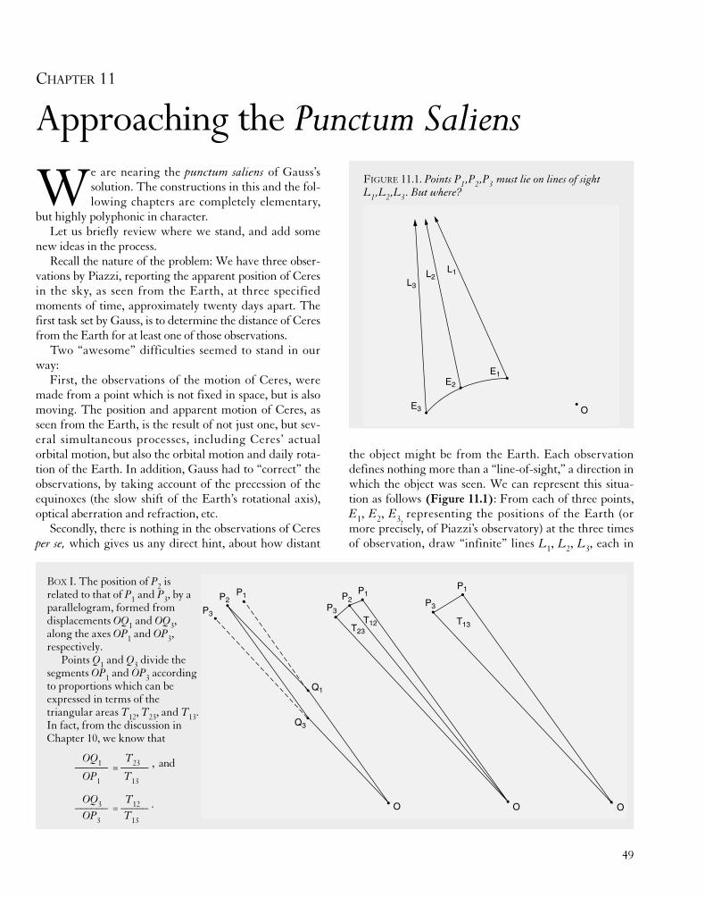
49

We are nearing the punctum saliens of Gauss’ssolution. The constructions in this and the fol-lowing chapters are completely elementary,

but highly polyphonic in character.Let us briefly review where we stand, and add some

new ideas in the process.Recall the nature of the problem: We have three obser-

vations by Piazzi, reporting the apparent position of Ceresin the sky, as seen from the Earth, at three specifiedmoments of time, approximately twenty days apart. Thefirst task set by Gauss, is to determine the distance of Ceresfrom the Earth for at least one of those observations.

Two “awesome” difficulties seemed to stand in ourway:

First, the observations of the motion of Ceres, weremade from a point which is not fixed in space, but is alsomoving. The position and apparent motion of Ceres, asseen from the Earth, is the result of not just one, but sev-eral simultaneous processes, including Ceres’ actualorbital motion, but also the orbital motion and daily rota-tion of the Earth. In addition, Gauss had to “correct” theobservations, by taking account of the precession of theequinoxes (the slow shift of the Earth’s rotational axis),optical aberration and refraction, etc.

Secondly, there is nothing in the observations of Ceresper se, which gives us any direct hint, about how distant

the object might be from the Earth. Each observationdefines nothing more than a “line-of-sight,” a direction inwhich the object was seen. We can represent this situa-tion as follows (Figure 11.1): From each of three points,E1, E2, E3, representing the positions of the Earth (ormore precisely, of Piazzi’s observatory) at the three timesof observation, draw “infinite” lines L1, L2, L3, each in

CHAPTER 11

Approaching the Punctum SaliensFIGURE 11.1. Points P1 ,P2 ,P3 must lie on lines of sightL1 ,L2 ,L3 . But where?

E1

E3

E2

O

L1L2L3

P1P2

P3

Q1

Q3

T13

P3

P1P2

P3

P1

T12T23

O O O

BOX I. The position of P2 isrelated to that of P1 and P3, by aparallelogram, formed fromdisplacements OQ1 and OQ3,along the axes OP1 and OP3,respectively.

Points Q1 and Q3 divide thesegments OP1 and OP3 accordingto proportions which can beexpressed in terms of thetriangular areas T12, T23, and T13.In fact, from the discussion inChapter 10, we know that

OQ1 T23______ = _____ , andOP1 T13

OQ3 T12______ = _____ .OP3 T13

50

the direction in which Ceres was seen at the correspond-ing time. Concerning the actual positions in space ofCeres (positions we have designated P1, P2, P3), the obser-vations tell us only, that P1 is located somewhere alongL1, P2 is somewhere on L2, and P3 is somewhere on L3.For an empiricist, the distances along those lines remaincompletely indeterminate.

We, however, know more. If Ceres belongs to thesolar system, its motion must be governed by the har-monic ordering of that system, as expressed (in part) bythe Gauss-Kepler constraints. Those constraints reflectthe curvature of the space-time, within which the eventsrecorded by Piazzi occurred, and relative to which wemust “read” his observations.

According to Gauss’s first constraint, the orbit of Ceresis confined to some plane passing through the center of thesun. This simple proposition, should already transformour “reading” of the observations. The three positions P1,P2, P3, rather than simply lying “somewhere” along therespective lines, are the points of intersections of the threelines L1, L2, L3 with a certain plane passing through thesun. (Figure 11.2a) We don’t yet know which plane thisis; but, the very occurrence of an intersection of that form,already greatly reduces the degree of indeterminacy of theproblem, and introduces a relationship between the three(as yet unknown) positions and distances.

Indeed, imagine a variable plane, which can pivotaround the center of the sun; for each position of thatplane, we have three points of intersection, with the linesL1, L2, L3. Consider, how the configuration of those three

points, relative to each other and the sun, changes as afunction of the variable “tilt” of the plane. (Figure 11.2b)Can we specify something characteristic about the geo-metrical relationship among the three actual positions P1,P2, P3 of Ceres, which might distinguish that specificgroup of points a priori from all other “triples” of points,generated as intersections of the three given lines with anarbitrary plane through the center of the sun?

Thanks to the work of the last chapter, we alreadyhave part of the answer. (Box I) We found, that the sec-ond position of Ceres, P2, is related to the first and thirdpositions P1 and P3, by the existence of a parallelogram,whose vertices are O, P2, and two points Q1 and Q3, lyingon the axes OP1 and OP3 respectively. Furthermore, wediscovered that the positions Q1 and Q3, defining thosetwo displacements, can be precisely characterized interms of ratios of the triangular areas spanned by thepositions P1, P2, P3 (and O).

Henceforth, we shall sometimes refer to the values ofthose ratios, T23 : T13 and T12 : T13 (or, T23 /T13 andT12 /T13), as “coefficients,” determining the interrelationof the three positions in question.

We already observed in the last chapter, that the trian-gular areas entering into these relationships, are nearlythe same as the orbital sectors swept out by the planet inmoving between the corresponding positions; and, whoseratios are known to us, thanks to Kepler’s “area law,” asratios of elapsed times. In fact, we calculated them in thelast chapter from Piazzi’s data.

The area of each orbital sector, however, exceeds that of

P3

P2

P1

E1

E3

E2

O

L1L2L3

P3

P2

P1

E1

E3

E2

O

L1L2L3

P3′

P2′P1′

FIGURE 11.2. (a) P1 ,P2 ,P3 , which are positions on Ceres’ orbit, must all lie in some plane passing through the sun. (b) Eachhypothetical position of the orbital plane defines a different configuration of positions P1 ,P2 ,P3 relative to each other.

(b)(a)

the corresponding triangle, by the lune-shaped area, en-closed between the orbital arc and the straight-line segmentconnecting the corresponding two positions of the planet.

As long as the three positions of the planet are relative-ly close together—as they are in the case of Ceres at thetimes of Piazzi’s observations—the lune-shaped excessesamount to only a small fraction of the areas of the trian-gles (or sectors). In that case, the ratios of the triangles T23 : T13 and T12 : T13 would be “very nearly” equal to theratios of the corresponding orbital sectors, S23 : S13 and S12 : S13, whose values we calculated in the precedingchapter.

Can we regard the small difference between the trian-gle and sector ratios, as an “acceptable margin of error”for the purposes of a first approximation? If so, then wecould take the numerical values calculated in Chapter 10from the ratios of the elapsed times, and say:

T23 S23____ = (approximately) ____ = 0.513 ,T13 S13

T12 S12____ = (approximately) ____ = 0.487 .T23 S23

Let us suppose, for the moment, that these equationswere exactly correct, or very nearly so. What would they tellus, about the configuration of the three points P1, P2, P3?

To get a sense of this, readers should perform the fol-lowing graphical experiment: Choose a fixed point O, torepresent the center of the sun, and choose any two otherpoints as hypothetical positions for P1 and P3. Next,determine the corresponding positions of Q1 and Q3 onthe segments OP1 and OP3, so that OQ1 is 0.513 times thetotal length of OP1, and OQ3 is 0.487 times the totallength of OP3. Combine the displacements OQ1 and OQ3according to the “parallelogram law,” to determine aposition for P2. Now, change the positions of P1 and P3,and see how P2 changes. What remains constant in therelationship between P2, P1, and P3? Also, examine theeffect, of replacing the “coefficients” just used, by someother pair of values, say 0.6 and 0.9.

Evidently, by specifying the values of the ratios in termsof which the position of P2 is determined by those of P1and P3, we have greatly restricted the range of “possible”triples of points, which could qualify as the three actualpositions for Ceres.

Recall the image of a manifold of “triples” of points,generated as the intersections of a variable plane, passingthrough the center of the sun, with the three “lines ofsight” L1, L2, L3. (SEE Figure 11.2) How many of thosetriples manifest the specific type of relationship of the sec-ond upon the first and third, defined by those specific val-ues for the coefficients? Exploring this question by draw-ings and examples, we soon gain the conviction, that—

apart from very exceptional cases in terms of the lines L1,L2, L3, and the specified values of the coefficients—thespecified type of configuration is realized for only oneposition of the movable plane. Thus, the positions of thethree points in question, are practically uniquely deter-mined, once L1, L2, L3 and the “coefficients” are given.

If that is the case, then the task we have set ourselvesmust, intrinsically, be capable of solution! In particular,there must be a way to determine the Earth-Ceres dis-tances from nothing more than the directions of the linesL1, L2, L3 (as given by Piazzi’s observations), the positionsof the Earth, and sufficiently accurate values for the coef-ficients defined above.

To see how this might be accomplished, reflect on theimplications of the parallelogram expressing the interre-lationship between the second, and the first and thirdpositions of Ceres. (SEE Box I) That parallelogramexpresses the circumstance, that the (as yet unknown)position of P2, results from a combination of the two dis-placements OQ1 and OQ3. Concerning the positions of Q1and Q3, we know that they lie on the segments OP1 andOP3, respectively, and divide those segments according toproportions (“coefficients”) whose values are known tous, at least in approximation. (Figure 11.3) Unfortunate-ly, since we don’t know P1 and P3, we have no way todirectly determine the positions of Q1 and Q3 in space.

Let us look into the situation more carefully. Consider,first, the displacement OQ1 in relation to the positions ofthe sun, Earth, and Ceres at the first moment of observa-tion. Those positions form a triangle, whose sides are

51

P1P2

P3

Q3

Q1

O

E2E1

E3

FIGURE 11.3. Closing in on P2 . The proportional rela-tionships of Q1 ,Q3 to OP1 ,OP3 are known approximatelyfrom the ratios of elapsed times.

52

OE1, OP1 and E1P1. (Figure 11.4a) Point Q1 lies on one ofthose sides, namely OP1, dividing it according to the pro-portion defined by the first coefficient. However, we can’tsay anything about the lengths of OP1 and E1P1, norabout the angle between them, so the position of Q1remains undetermined for the moment.

But what about the points, which correspond to Q1 onthe other sides of the triangle? Draw the parallel to theline-of-sight E1P1, through Q1 down to OE1. That parallelintersects the axis OE1 at a location, which we shall call F1.That point F1 will divide the segment OE1 by the sameproportion, that Q1 divides OP1 (for, by construction,

BOX II. The position of P2 results from the combination ofthe displacements OQ1 and OQ3 . On the other hand, by ourconstructions,

OQ1 = OF1 + F1Q1, and OQ3 = OF3 + F3Q3.

Combine displacements OF1 and OF3, to get a position F,and then perform the other two displacements, F1Q1 and

F3Q3. This amounts to constructing a parallelogram based atF whose sides are parallel to, and congruent with, thesegments F1Q1 and F3Q3. The directions of the lattersegments are parallel to Piazzi’s “lines of sight” from E1 toP1 and E3 to P3, respectively. The end result must be P2. Thistells us that P2 lies in the plane through F, determined bythose two “line of sight” directions.

P1P2

P3

Q3

Q1

O

G3

E2

G1

E1

E3 F3

F1F

Q3

Q1

P2

F1

F3

F

O

L3′

L1′

FIGURE 11.4. Closing inon P2 . Determining (a) F1 and the directionof F1Q1 , and (b) F3 andthe direction of F3Q3 .

P3

Q3

F3

G3

E3 O

P1

Q1

G1

F1

E1

O

(a) (b)

OF1Q1 and OE1P1 are similar triangles). That proportion,as we noted, is at least approximately known. Since theposition of the Earth, E1, is known, we can determine theposition of F1 directly, by dividing the known segment OE1according to that same proportion.

This result brings us, by implication, a dimension clos-er to our goal! Observe, that—by construction—the seg-ment F1Q1 is parallel to, and congruent with, a sub-seg-ment of the line-of-sight E1P1. Call that sub-segmentE1G1. In other words, to arrive at the location of Q1 fromO, we can first go from O to the position F1, just con-structed, and then carry out a second displacement,equivalent to the displacement E1G1 but applied to F1instead of E1. We don’t know the magnitude of that dis-placement, but we do know its direction, which is that ofthe line of sight L1 given by Piazzi’s first observation.

Now, apply the very same considerations, to the posi-tions for the third moment of observation (i.e., the trian-gle OE3P3). (Figure 11.4b) Dividing the segment OE3according to the value of the second coefficient, deter-mine the position of a point F3 on the line OE3, such thatthe line F3Q3 is parallel with the line-of-sight E3 P3. Thedisplacement OQ3 is thus equivalent to the combinationof OF3, and a displacement in the direction defined by theline of sight E3P3, i.e., L3.

We are now inches away from being able to determinethe position of P2! Recall, that we resolved the displace-ment OP2 into the combination of OQ1 and OQ3. Each ofthe latter two displacements, on the other hand, has now

been decomposed, into a known displacement (OF1 andOF3, respectively), and a displacement along one of thedirections determined by Piazzi’s observations. In otherwords, OP2 is the result of four displacements, of whichtwo are known in direction and length, and the other twoare known only as to direction. (Box II)

Assuming, as we did from the outset, that the result ofa series of displacements of this type, does not sensibly dependon the order in which they are combined, we can imaginecarrying out the four displacements, yielding the positionof P2 relative to O, in the following way: First, combinethe displacements OF1 and OF3. The result is a point F,located in the plane of the ecliptic. We can determine theposition of F directly from the known positions F1 andF3. Then, apply the two remaining displacements, to getfrom F to P2.

What does that say, about the nature of the relation-ship of P2 to F? We don’t know the magnitudes of thedisplacements carrying us from F to P2, but we knowtheir two directions. They are the directions defined byPiazzi’s original lines of sight, L1 and L3. Aha! Those twodirections, as projected from F, define a specific planethrough F. We have only to draw parallels L1′ , L3′through F, to the just-mentioned lines of sight; the planein question, plane Q, is the plane upon which L1′ and L3′lie. (Figure 11.5) Since that plane contains both of thedirections of the two displacements in question, theircombined result, starting from F—i.e., P2—will in any

53

FIGURE 11.5. P2 must lie on plane Q constructed at point F.But where?

plane Q

L3

L1

E1

E2

E3

F

O

?L3′

L1′

L3

L2

E3

E2

L1

F

P2 !

E1

plane Q

L3′L1′

FIGURE 11.6. Locating P2 . Line L2 , originating at E2 ,must intersect plane Q at point P2 . E2 P2 is the crucialdistance we are seeking.

54

case be some point in that plane.So, P2 lies on that plane. But where? Don’t forget the

second of the selected observations of Piazzi! That obser-vation defines a line L2, extended from E2, along whichP2 is located. Where is it located? Evidently, at the point ofintersection of L2 with the plane which we just constructed!(Figure 11.6) The distance along L2, between E2 andthat point of intersection (i.e., the distance E2 P2), is thecrucial distance we are seeking. Eureka!

This—with one, very crucial addition by Gauss—defines the kernel of a method, by which we can actuallycalculate the Earth-Ceres distance. It is only necessary totranslate the geometrical construct, just sketched, into a

form which is amenable to precise computations.However, the pathway of solution we have found so

far, has one remaining flaw. We shall discover that, andGauss’s ingenious remedy, in Chapter 12.

In the meantime, readers should ponder the following:The possibility of determining the position of P2, as theintersection of the line L2 with a certain plane through F,presupposes, that F does not coincide with the origin ofthat line, namely E2. In fact, the size of the gap between Fand E2, reflects the difference in curvature between theorbits of Earth and Ceres, over the interval from the firstto the third observations.

—JT

CHAPTER 12

An Unexpected Difficulty Leads toNew Discoveries

In Chapter 11, we appeared to have won a major bat-tle in our efforts to determine the orbit of Ceres fromthree observations. The war, however, has not yet

been won. As we soon shall see, the greatest challengestill lies before us.

We developed a geometrical construction that gives us

an approximation for the second position of Ceres. Thatconstruction consisted of the following essential steps:

1. The three chosen observations define the directions ofthree “lines-of-sight” from Piazzi’s observatorythrough the positions of Ceres, at each of the giventimes of observation. Using that information, and theknown orbit and rotational motion of the Earth, deter-mine the positions of the observer, E1, E2, E3, and con-struct lines L1, L2, L3, running from each of those posi-tions in the corresponding directions.* (Figure 12.1)

2. From the times provided for Piazzi’s observations,compute the ratios of the elapsed times, between thefirst and second, the second and third, and the first andthird times—i.e., the ratios t2−t1: t3−t1 and t3−t2: t3−t1.

3. According to Kepler’s “area law,” the values, just com-puted, coincide with the ratios of the sectoral areas,S12 : S13 and S23 : S13, swept out by Ceres over the corre-sponding time intervals. We assumed, that for the pur-

_________* For reference, Piazzi gave the apparent positions for Jan. 2, Jan. 22,

and Feb. 11, 1801, as follows:

right ascension declinationJan. 2 51º 47′ 49″ 15º 41′ 5″Jan. 22 51º 42′ 21″ 17º 3′ 18″Feb. 11 54º 10′ 23″ 18º 47′ 59″

Those “positions” are nothing but the directions in which the linesL1, L2, L3 are “pointing.”

E1

E2

E3

P3

P2P1

O

L1L2

L3

FIGURE 12.1. Relationships of the positions of the sun (O),Earth (E1 ,E2 ,E3 ), lines of sight, and Ceres (P1 ,P2 ,P3 ).

OE3, according to the ratios defined by theapproximate values for the coefficients c and d. Inother words, construct points F1 and F3, along thesegments OE1 and OE3, respectively, in such a way, thatOF1/OE1 = t3−t2 / t3−t1 and OF3 /OE3 = t2−t1 / t3−t1.Then, construct F as the endpoint of the resultant ofthe two displacements OF1 and OF3. (Thus, F will bethe fourth vertex of the parallelogram constructedfrom points O, F1, and F3.) (Figure 12.3)

6. Next, draw lines L1′, L3′ parallel to the lines L1 and L3,through F. The resulting lines determine a uniqueplane, Q, passing through F.

7. Determine the point P, where the line L2 intersects theplane Q. In other words, “project” from the secondposition E2 of the Earth, along the “line of sight”defined by the second observation, until you hit theplane Q. (Figure 12.4) That point, P, is our firstapproximation for the Ceres position P2!

55

pose of approximation, it would be possible to ignore therelatively small discrepancy between the ratios of the or-bital sectors on the one hand, and those of the correspond-ing triangular areas formed by the sun and the corre-sponding positions of Ceres, on the other. (Figure 12.2)

4. On that basis, we assumed that the ratios of the elapsedtimes, computed in step 2, provide “sufficiently pre-cise”approximations to the values for the ratios of thetriangular areas, T12 : T13 and T23 : T13. The true valuesof those ratios, which I shall refer to as “d” and “c,”respectively, are the coefficients which define the spa-tial relationship of the second position of Ceres to thefirst and third positions, in terms of the “parallelogramlaw” for the combination and decomposition of simpledisplacements in space.

5. Using the approximate values for c and d adducedfrom the elapsed times in the manner just described,construct a position F, in the plane of the Earth’s orbit,in such a way, that F’s relationship to the Earth positionsE1 and E3 , is the same as that adduced to exist between thesecond, and first and third positions of Ceres.

To spell this out just once more: Divide the lengthsof the segments from the sun to the Earth, OE1 and

P3

P2 P1

O

P3

P2 P1

O

P3

P2 P1

S23

S12

S13

T23

T12

T13

O

O

P3

P2 P1

O

E2E1

E3 F3

F1F

L3

L2

E3

E2

L1

F

P2 !

E1

plane Q

L3′L1′

FIGURE 12.2. Orbital sectors S12 ,S23 ,S13 and correspondingtriangular areas T12 ,T23 ,T13 .

FIGURE 12.4. The intersection of line L2 with plane Q,determines point P2 .

FIGURE 12.3. Determining point F, as a combination ofdisplacements along OE1 and OE3 .

56

Using routine methods of analytical and descriptivegeometry, as developed by Fermat and perfected by Gas-pard Monge et al., we can translate the geometrical con-struction, sketched above, into a procedure for numericalcomputation of the distance E2P, from the data providedby Piazzi.

We would be well advised, however, to think twicebefore launching into laborious calculation. As it stands,our method is based on a crude approximation for esti-mating the values of the crucial coefficients, c and d.Remember, we chose to ignore the differences betweenthe orbital sectors and the corresponding triangles. Wemight argue for the admissibility of that step, for the pur-poses of approximation, as follows.

Firstly, we are concerned only with the ratios, andnot the absolute magnitudes of the sectors and triangles.Secondly, the differences in question—namely the lune-shaped areas contained between the orbital arcs and thestraight-line chords connecting the correspondingorbital positions—are certainly only a tiny fraction ofthe total areas of the orbital sectors. Hence, they willhave only a “marginal” effect on the values of the ratiosof those areas.

In fact, simple calculations, carried out for the hypo-thetical assumption of a circular orbit between Mars andJupiter,* indicate, that we can expect an error on theorder of about one-fourth of one percent in the determina-tion of the coefficients c and d, when we disregard the

difference between the sectors and the triangles. Not bad,eh?

Before celebrating victory, however, let us look at thepossible effect of that magnitude of error in the coeffi-cients, for the rest of the construction.

Look at the problem more closely. An error of x per-cent in the values of c and d, will produce a correspond-ing percentual error in the positions of F1 and F2, and atmost twice that error, in the process of combining OF1and OF3 to create F. Any error in the position of F, how-ever, produces a corresponding shift in the position ofthe plane Q, whose intersection with L2 defines ourapproximation to the position of Ceres. Now, the direc-tions of the lines L1, L2, L3, which arose from observa-tions made over a relatively short time, differ only by afew degrees. Since the orientation of the plane Q isdetermined by parallels to L1 and L3 at F, this meansthat L2 will make an extremely “flat” angle to the planeQ. A slight shift in the position of the plane, yields amuch larger change in the location of its intersection withL2. How much larger? If we analyze the relative config-uration of L2, Q, and the ecliptic, corresponding to thesituation in Piazzi’s observations, then it turns out thatany error in the position of F, can generate an error tento twenty times larger in the location of the intersection-point. (Figure 12.5) That would bring us into the rangeof a worrisome 5-10 percent error in our estimate for theEarth-Ceres distance E2 P2.

__________

* To get a sense, how large that supposedly “marginal” error mightbe, let us work out a hypothetical case. Suppose that the unknownplanet were moving in a circular orbit, about halfway betweenMars and Jupiter; say, at a distance of 3 Astronomical Units(A.U.) from the sun (three times the mean Earth-sun distance).According to Kepler’s constraints, the square of the periodic time(in years) of any closed orbit in the solar system, is equal to thecube of the major axis of the orbit (in A.U.). The periodic time forthe unknown planet, in this case, would be the square root of3�3�3, or about 5.196152 (years). In a period of 20 days (i.e.,approximately the time between the successive observationsselected by Gauss), the planet would traverse a certain fraction ofa total revolution around the sun, equivalent to 20 divided by thenumber of days in the orbital period of 5.196152 years, i.e.,20/(365.256364 � 5.196152), or 0.010538. To find the area of theorbital sector swept out during 19 days, we have only to form theproduct of 0.010538 and the area enclosed by a total revolution—the latter being equal to π (�3.141593) times the square of theorbital radius (3�3). We get a result of 0.297951, in units ofsquare A.U.

Next, compute the triangular area between the sun and twopositions of the planet, 20 days apart. The angle swept out at thesun by that motion, is 0.010538 � 360º, or 3.79368º. The height andbase of the corresponding isosceles triangle, whose longer sides areequal to the orbital radius, can be estimated by graphical means, orcomputed with the help of sines and cosines. The triangle is found

to have a height of 2.998356 A.U. and a base (the chord betweenthe two planetary positions) of 0.198600 A.U., for an area of0.297737 square A.U.

Comparing the values just obtained, we find the excess area ofthe orbital sector over the triangle, to be a “mere” 0.000214 squareA.U. (Given that an astronomical unit is 150 million kilometers,that “tiny” area corresponds to “only” about 5 trillion square kilo-meters!) More to the point, the ratio of the sector to the triangulararea is 1.000718. Thus, in replacing the triangular areas T12 andT23 by the corresponding sector areas S12 and S23, in the ratioswhich define the coefficients c and d, we introduce an error ofabout 0.07 percent.

Note, however, that these estimates only apply to an elapsedtime of the order of 20 days—such as between the first and sec-ond, and the second and third positions. The first and third posi-tions, on the other hand, are about 40 days apart; calculating thiscase through, we find an orbital sector area of 0.595902 and a tri-angular area of 0.594170 square A.U. In this case, the difference is0.00193 square A.U.—almost eight times what it was in the earliercase!—and the ratio is 1.0029, corresponding to a proportionalerror of more than 0.29 percent. This is the error to be expected,when we use S13 instead of T13 in the ratios defining the coeffi-cients c and d.

From these exploratory computations, we conclude that by farthe largest source of error, in our estimate of the coefficients c andd, is due to the discrepancy between S13 and T13.

57

As a matter of fact, our calculation with circular orbitsgreatly underestimates the error in the coefficients c and d,which would occur in the case of a significantly non-circu-lar orbit (as is the case for Ceres). In that case, the errorcan amount to 2 percent or more, leading to a final errorof 20-30 percent in our estimate of the object’s distance.

Such a huge margin of error would render any predic-tion of the position of Ceres completely useless.

Back to CurvatureReality has rejected the crudeness of our approach, in try-ing to ignore the discrepancies between the orbital sectorsand the corresponding triangles. Those discrepancies are,in fact, the most crucial characteristics of the orbit itself

“in the small”; they result from the curvature of the orbit,as reflected in the elementary fact, that the path of theplanet between any two points, no matter how closetogether, is always “curving away from” a straight line.*

To come to grips with the problem, no less than threelevels of the process must be taken into account:

(i) The curvature “in the infinitely small,” which actsin any arbitrarily small interval, and continuously“shapes” the orbit at every moment of an ongoing processof generation.

(ii) The curvature of the orbit “in the large,” consid-ered as a “completed” totality “in the future,” and whichironically pre-exists the orbital motion itself; this, of courseas defined in the context of the solar system as a whole.

(iii) The geometrical intervals among discrete loci P1,P2, etc., of the orbit, as moments or events in the process,and whose relationships embody a kind of tensionbetween the apparent cumulative or integrated effect ofcurvature “in the small,” and the curvature “in thelarge”—acting, as it were, from the future.

Euler, Newton, and Laplace rejected this, linearizingboth in the small and in the large. From the standpoint ofNewton and Laplace, the orbit as a whole—history!—hasno efficient existence. An orbit is only the accidental traceof a process which proceeds “blindly” from moment tomoment under the impulse of momentary “forces”—likethe “crisis management” policies of recent years! For theNewtonian, only “force”, which you can “feel” in the“here and now,” has the quality of reality. But Newtonian“blind force” is a purely linear construct, devoid of cogni-tive content. You can travel the entropic pathway of deriv-ing the “force law” algebraically from Kepler’s Laws; but,in spite of elaborate efforts of Laplace et al., it is axiomati-cally impossible to derive the Keplerian ordering of thesolar system as a whole, from Newton’s physics.

In fact, the efforts of Burkhardt and others, to deter-mine the orbit of Ceres using the elaborate mathematicalapparatus set forth by Laplace in his famous MéchaniqueCéleste, proved a total failure. According to the report ofGauss’s friend, von Zach, the elderly Laplace, who—from the lofty heights of Olympus, as it were—had beenfollowing the discussions and debates concerning Ceres,concluded that it was impossible to determine the orbit

L2

F

P2

plane Q′plane Q

F′

P2′

FIGURE 12.5. Owing to the extremely flat angle which theline L 2 makes to the plane Q, a slight shift in the position ofF (from F to F′ ) causes a much larger change in the pointof intersection with L 2 (from P2 to P2′ ).

__________

* Industrious readers, who took the trouble to actually plot the posi-tion of F, using the ratios of elapsed times as described above, willhave discovered, that F lies on the straight line between E1 and E3.One might also note the following:

(i) As long as we use the ratios of elapsed times as our coeffi-cients, the sum of those coefficients will invariably be equal to 1.

(ii) If we have any two points A and B, divide the segments OA

and OB according to coefficients whose sum is equal to 1, and gen-erate the corresponding displacements along those two axes. Thepoint resulting from the combination of those displacements, willalways lie along the straight line joining A and B.

(iii) Consequently, insofar as P2 does not lie on the segment P1P3,in virtue of the curvature of Ceres’ orbit, the sum of the true valuesof c and d, will always be different from, and, in fact, greater than 1.

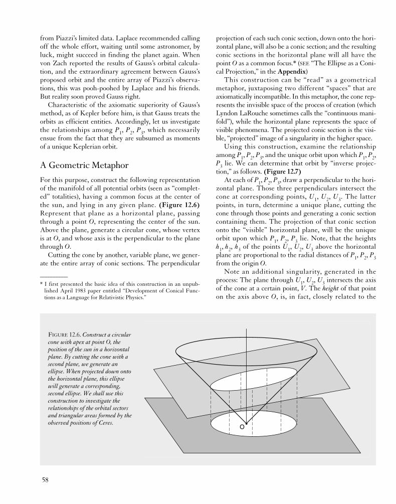
58

from Piazzi’s limited data. Laplace recommended callingoff the whole effort, waiting until some astronomer, byluck, might succeed in finding the planet again. Whenvon Zach reported the results of Gauss’s orbital calcula-tion, and the extraordinary agreement between Gauss’sproposed orbit and the entire array of Piazzi’s observa-tions, this was pooh-poohed by Laplace and his friends.But reality soon proved Gauss right.

Characteristic of the axiomatic superiority of Gauss’smethod, as of Kepler before him, is that Gauss treats theorbits as efficient entities. Accordingly, let us investigatethe relationships among P1, P2, P3, which necessarilyensue from the fact that they are subsumed as momentsof a unique Keplerian orbit.

A Geometric MetaphorFor this purpose, construct the following representationof the manifold of all potential orbits (seen as “complet-ed” totalities), having a common focus at the center ofthe sun, and lying in any given plane. (Figure 12.6)Represent that plane as a horizontal plane, passingthrough a point O, representing the center of the sun.Above the plane, generate a circular cone, whose vertexis at O, and whose axis is the perpendicular to the planethrough O.

Cutting the cone by another, variable plane, we gener-ate the entire array of conic sections. The perpendicular

projection of each such conic section, down onto the hori-zontal plane, will also be a conic section; and the resultingconic sections in the horizontal plane will all have thepoint O as a common focus.* (SEE “The Ellipse as a Coni-cal Projection,” in the Appendix)

This construction can be “read” as a geometricalmetaphor, juxtaposing two different “spaces” that areaxiomatically incompatible. In this metaphor, the cone rep-resents the invisible space of the process of creation (whichLyndon LaRouche sometimes calls the “continuous mani-fold”), while the horizontal plane represents the space ofvisible phenomena. The projected conic section is the visi-ble, “projected” image of a singularity in the higher space.

Using this construction, examine the relationshipamong P1, P2, P3, and the unique orbit upon which P1, P2,P3 lie. We can determine that orbit by “inverse projec-tion,” as follows. (Figure 12.7)

At each of P1, P2, P3, draw a perpendicular to the hori-zontal plane. Those three perpendiculars intersect thecone at corresponding points, U1, U2, U3. The latterpoints, in turn, determine a unique plane, cutting thecone through those points and generating a conic sectioncontaining them. The projection of that conic sectiononto the “visible” horizontal plane, will be the uniqueorbit upon which P1, P2, P3 lie. Note, that the heightsh1, h2, h3 of the points U1, U2, U3 above the horizontalplane are proportional to the radial distances of P1, P2, P3from the origin O.

Note an additional singularity, generated in theprocess: The plane through U1, U2, U3 intersects the axisof the cone at a certain point, V. The height of that pointon the axis above O, is, in fact, closely related to the

__________

* I first presented the basic idea of this construction in an unpub-lished April 1983 paper entitled “Development of Conical Func-tions as a Language for Relativistic Physics.”

FIGURE 12.6. Construct a circularcone with apex at point O, theposition of the sun in a horizontalplane. By cutting the cone with asecond plane, we generate anellipse. When projected down ontothe horizontal plane, this ellipsewill generate a corresponding,second ellipse. We shall use thisconstruction to investigate therelationships of the orbital sectorsand triangular areas formed by theobserved positions of Ceres.

O

“parameter” of the orbit, which played a key role inGauss’s formulation of Kepler’s constraints. Gaussshowed, that the area swept out by a planet in its motionin a given orbit over any interval of time, is proportional(by a universal constant of the solar system) to the dura-tion of the time interval, multiplied by the square root ofthe “orbital parameter.” Integrating this with the conicalrepresentation that we have just introduced, opens up anew pathway toward the solution of our problem.

In fact, if we cut the cone horizontally at the height ofV, then the intersection of that horizontal with the planeof U1, U2, U3, will be a line l, perpendicular to the mainaxis of the conic section. That line l intersects the conicsection in two points, which lie symmetrically on oppositesides of V and at the same height. The segment l′ of l(bounded by those points) defines the cross-width of theconic section at V. Line segment l′ is also a diameter ofthe cone’s circular cross-section at V, which in turn is pro-portional to the height h of V on the axis. Now, projectdown to the horizontal plane of P1, P2, P3. The image ofl′, equivalent to l′ in length, is the perpendicular diameterof the orbit at the focus O, exactly the length that Gausscalled the “parameter” of the orbit.

All of this can be seen, nearly at a glance, from the dia-gram in Figure 12.6. The immediate upshot is, thatGauss’s “orbital parameter,” which governs the relation-ship between the elapsed time and the area swept out bythe motion of a planet in its orbit, is proportional to theh of the point V on the axis of the cone.

On the other hand, our method of “inverse projection”allows us to determine V directly in terms of the threepositions P1, P2, P3, by constructing the plane through thecorresponding points U1, U2, U3. As a “spin-off” of theseconsiderations, we obtain a simple way to determineGauss’s orbital parameter for any orbit, from nothingmore than the positions of any three points on the orbit.We can say even more, however.

We found, earlier, a way to express the spatial rela-tionship between P1, P2, P3 (relative to O), in terms ofthe ratios of the triangular areas T12, T23, T13. Thispoints to the existence of a simple functional relationshipbetween those triangular areas, and the value of theorbital parameter (or, equivalently, the height of V ).The latter, in turn, is functionally related to the valuesof corresponding times and orbital sectors, by Gauss’sconstraint. (Figure 12.8)

Our conical construction has provided a missing link,in the necessary coherence of the orbital sectors with thecorresponding triangles. This, in turn, will allow us tosupersede the crude approximation, used so far, and todetermine the Ceres distance with a precision whichLaplace and his followers considered to be impossible.

The details will be worked out in the following chap-ter. But, it is already clear, that we have advanced byanother, critical dimension, closer to victory. The key toour success, was a sortie into the “continuous manifold”underlying the planetary orbits.

—JT

59

FIGURE 12.7. Use our construction to relate positionsP1 ,P2 ,P3 , radial distances r1 ,r2 ,r3 , heights h and h1 ,h2 ,h3 ,and the orbital parameter.

OP2

P3

V

l

l′

P1

U1

U3

U2

orbitalparameter

h3h2h h1

r3r2

r1

FIGURE 12.8. What is the relationship between thetriangular areas T12 , T23 , T13 and height h of the point V?

OP2

P3

V

P1

U1

U3

U2

T12

T23

h

60

In the previous chapter, we shifted our attention fromthe visible form of Ceres’ orbit, to its generation in ahigher domain. With the help of a simple geometri-

cal metaphor, we represented the higher domain by a cir-cular cone with its axis in the vertical direction, and thelower, “visible domain” by a horizontal plane. We madethe plane intersect the cone at its vertex, at the locationcorresponding to the center of the sun, and likened therelationship of visible events to events in the higher, “con-ical space,” to a projection from the cone, parallel to theconical axis, down to the plane.

In fact, if we trace Ceres’ orbit on the horizontal plane,that form is the projected image of a conic section on thecone.

How is it possible to use the geometry of visual space,to “map” relationships in a “higher space” of an axiomati-cally different character? Only as paradox. Obviously, no“literal” representation is possible, nor do we have a mereanalogy in mind. When we represent visual space by atwo-dimensional plane (inside visual space!), and the high-er space as a cone in “three dimensions,” projected ontothe plane, we do not mean to suggest that the higherspace is only “higher” by virtue of its having “moredimensions.” Rather, we should “read” the axis of thecone in our representation, to signify a different type ofordering principle than that of visual space—oneembodying features of the transfinite, “anti-entropic”ordering of the Universe as a whole.

Reflecting on the irony of applying constructions ofelementary geometry to such a metaphorical mapping,the following idea suggests itself: The geometry of visiblespace has shown itself appropriate to a process of discoveryof the reality lying outside visual space, when it is consid-ered not as something fixed and static, but as constantlyredefined and developed by our cognitive activity, just aswe develop the well-tempered system of music throughClassical thorough-composition. Should we not treat ele-mentary geometry from the standpoint, that visual spaceis created and “shaped” to the purpose of providing reasonwith a pathway toward grasping the “invisible geometry”of Creation itself?

Keeping these ironies in mind, let us return to thechallenge which last chapter’s discussion placed in frontof us. We developed a method for constructing an

OP2

P3

V

l

l′

P1

U1

U3

U2

orbitalparameter

h

S12

S23

CHAPTER 13

Grasping the Invisible Geometry Of Creation

approximation of Ceres’ position, which did not ade-quately take into account the space-time curvature in thesmall. As a result, we introduced a source of error whichcould lead to major discrepancies between our estimateof the Earth-Ceres distance, and the real distance. IfGauss had not corrected that fault, his attempt at fore-casting the orbit of Ceres, would have been a failure.

We have no alternative, but to investigate the curva-ture in the small which characterizes the spatial relation-ship between any three positions P1, P2, P3 of a planet,solely by virtue of the fact that they are “moments” of oneand the same Keplerian orbit. And, to do that withoutany assumption concerning the particular form of theconic-section orbit.

We projected the three given positions up to the cone,to obtain points U1, U2, U3. The latter three points deter-mine a unique plane, which intersects the cone in a conicsection, and whose projection onto the horizontal plane isthe visible form of Ceres’ orbit. The intersection of thatsame plane with the axis of the cone, at a point we calledV, is an important singularity. The circular cross-sectionof the cone at the “height” of V, is cut by the U1U2U3

FIGURE 13.1. The orbital parameter is the projection ofdiameter l ′ in the circular cross-section of the cone at heighth of V. Diameter l ′ is generated by the intersection of thecircular and elliptical cross-sections.

61

plane at two points, which are the endpoints of a diame-ter l′ through V. That diameter projects (without changeof length) to the segment which represents the width ofthe Ceres’ orbit, measured perpendicularly to the axis ofthe orbit at its focus O. That length is what Gauss callsthe “orbital parameter.” (Figure 13.1)

Thus, Gauss’s parameter is equal to the cross-sectiondiameter of the cone at V, which, in turn, is proportional tothe height of V on the conical axis. The factor of propor-tionality depends upon the apex angle of the cone; that fac-tor becomes equal to 1, if we choose the apex angle of thecone to be 90° (so that the surface of the cone makes anangle of 45° with the horizontal plane at O). Let us choosethe apex angle so. In that case, the height h of V above theaxis is equal to half the orbital parameter. (Figure 13.2)

Now recall, that according to Gauss’s recasting ofKepler’s constraints, the area swept out by the planet inany time interval, is proportional to the elapsed time,multiplied by the square root of the half-parameter. (SEE

Chapter 8) Our analysis actually showed, that the con-stant of proportionality is π, when the elapsed time ismeasured in years, length in Astronomical Units (A.U.)(Earth-sun distance), and area in square A.U.

From these considerations, we can now express theareas of the orbital sectors of Ceres, in terms of the elapsedtimes and the height h of V on the cone. For example:

S12 = √_h � π� (t2−t1) , and

S23 = √_h � π� (t3−t2) .

At the close of the last chapter, we remarked that the

O

V

45°

orbital parameter

h

b a

FIGURE 13.2. Relationship of height h to the orbitalparameter. The diagram represents the cross-sectional “cut”of the cone, by the plane defined by the vertical axis and thesegment l′ (represented here as the segment between points aand b). Since the apex angle of the cone is 90°, the trianglesaVO and bVO are isosceles right triangles. Consequently, h = aV = bV = (1/2) � (length of ab) = half-parameter oforbit.

OP2

P3

V

P1

U1

U3

U2

T12

T23

h

value of h must somehow be expressible in terms of thetriangular areas T12, T23, T13; and, that the resulting linkwith S12 and S23, via h, would finally provide us with amuch more “fine-tuned” approximation to the crucialratios T12 : T13 and T23 : T13 than was possible on the basisof our initial, crude approach. (Figure 13.3)

Not to lose your conceptual bearings at this point,before we launch into a crucial battle, remember the fol-lowing: The significance of the orbital parameter, nowrepresented by h, lies in the fact that it embodies the rela-tionship between

(i) the Keplerian orbit as a whole;(ii) the array of “geometrical intervals” between any

three positions P1, P2, P3 on the orbit; and(iii) the curvature of each arbitrarily small “moment

of action” in the planet’s motion, as expressed in the cor-responding orbital sector, and above all in the relation-ship between the “curved” sectoral area and correspond-ing triangular area.

Gauss focussed his attention on the sector and triangleformed between the first and the third positions, S13 andT13. Our experimental calculations, reviewed in the lastchapter, indicated that the discrepancy between thesetwo, is the main source of error in our method for calcu-lating the Earth-Ceres distance. Hence, Gauss looked fora way to accurately estimate that area.

Gauss noted that most of the excess of S13 over T13, i.e.,the lune-shaped area between the orbital arc from P1 toP3 and the segment P1P3, is constituted by the triangular

FIGURE 13.3. Our conical projection, which contains both thetriangular areas and the elliptical sectors as well as the orbitalparameter h, will help us to devise a “fine-tuned”approximation to the crucial coefficients required todetermine the orbit of Ceres (cf. Figure 13.1).

area P1P2 P3. Denote this triangle—the triangle formedbetween all three positions of the planet—by “T123.”Gauss also observed, that T123 is the excess of T12 and T23combined, minus T13. (Figure 13.4)

How will our exploration of conical geometry help usto get a grip on that little “differential” T123? We voicedthe expectation, earlier, that “the height h of V on thecone must somehow be expressible in terms of the trian-gular areas T12, T23, T13.” The time has come, to makegood on our promise.

An Elementary Proposition of Descriptive GeometryThose brought up in the geometrical culture of Fermat,Desargues, Monge, Carnot, and Poncelet would experi-ence no difficulty whatever at this point. But, most of ustoday, emerged from our education as geometrical illiter-ates.* With a bit of courage, however, this condition canbe remedied.

Recall how we used the triangular areas T12, T13, andT23 to measure the relationship between the Ceres positionP2 and P1 , P3, as a combination of displacements along theaxes OP1 and OP3. Evidently, we touched upon a principleof geometry relevant to a much broader domain.

The nature of the relationship we are looking for now,becomes most clearly apparent, if we put Piazzi’s observa-tions aside for the moment, and examine, instead, thehypothetical case, where the P1, P2, P3 are widely separat-ed—say, at roughly equal angles (i.e., roughly 120° apart)around O. (Figure 13.5) In this case, we have a triangleP1P2P3 in the horizontal plane, which contains the point Oand is divided up by the radial lines OP1, OP2, OP3 into the

62

smaller triangles T12, T23, and T31. Above the triangleP1P2P3, and projecting exactly onto it, we have the triangleU1U2U3. This latter triangle “sits on stilts,” as it were, overthe former. The “stilts” are the vertical line segments P1U1,P2U2, and P3U3, whose heights are h1, h2, and h3. Point V isthe place where the axis of the cone passes through triangleU1U2U3. How does the height of V above the horizontalplane, depend on the heights h1, h2, and h3?

This is an easy problem for anyone cultured in syn-thetic geometry, rather than the stutifying, Cartesianform of textbook “analytical geometry” commonlytaught in schools and universities. The approach calledfor here, is exactly the opposite of “Cartesian coordi-nates.” Don’t treat the array of positions, and the organi-zation of space in general, as a dead, static entity. Think,instead, in physical terms; think in terms of change, dis-placement, work. For example: What would happen tothe height of V, if we were to change the height of one ofthe points U1, U2, U3?

Suppose, for example, we keep U2 and U3 fixed, whileraising the height of U1 by an arbitrary amount “d,” rais-ing it in the vertical direction to a new position U1′. (Fig-ure 13.6) The new triangle U1′U2U3 intersects the axis ofthe cone at a point V′, higher than V. Our immediate taskis to characterize the functional relationship between theparallel vertical segments VV′ and U1U1′.

The two triangles U1U2U3 and U1′U2U3 share thecommon side U2U3, forming a wedge-like figure. Cutthat figure by a vertical plane passing through the seg-ments VV′ and U1U1′. The intersection includes the seg-ment U1U1′ , and the lines through U1 and V, and

FIGURE 13.4. Most of the excess of S13 over T13 , which isthe lune-shaped area, is constituted by triangle T123 .

T13

T123

OO

P3

P2 P1

P3

P2 P1

U2 U3

h3

P3

h2

P2

P1

U1

h1 h

T23

T12T31

V

__________

* Including the present author, incidentally.

FIGURE 13.5. How does the height h of V depend uponheights h1 ,h2 ,h3 , which are in turn a function of theposition of the plane through U1 ,U2 ,U3 ?

through U1′ and V′, respectively, which meet each otherat some point M on the segment U2U3. Two triangles areformed in the vertical plane from those vertices:U1MU1′, and a sub-triangle VMV′ . Given that VV′ isparallel to U1U1′, those two triangles will be similar toeach other.

The ratio of similarity of these triangles, determinesthe relationship of immediate interest to us, namely, thatbetween the change in height of V (i.e., the length of VV′ )and the change in the height of U1 (i.e., the length ofU1U1′ ).

To determine the ratio of similarity of the triangles,we need only establish the proportionality between anypair of corresponding sides. So, look at the ratioMV : MU1, i.e., the ratio by which V divides the segmentMU1. That ratio is not changed when we project the seg-ment onto the plane of P1, P2, P3. Under the projection,U1 projects to P1, V projects to O, and M projects to somepoint N on the line P2P3.

Our problem is reduced to determining the ratio bywhich O divides the line segment NP1—that latter beingthe projected image of the segment MU1. Very simple!Look at P2P3 as the base of the triangle P1P2P3. (Figure13.7) Draw the line parallel to P2P3 through P1. The dis-tance separating that line and P2P3 is called the altitude ofthe triangle P1P2P3, whose product with the length of thebase, P2P3, is equal to twice the area of the triangle T123.Next, draw the parallel to P2P3 through the point O. Thegap between that line and P2P3, is the altitude of the tri-angle OP2P3, whose product with the length of the baseP2P3 is equal to twice the area of triangle T23.

Thus, the ratio of the distances between the first andsecond, and the first and third—that is, of the distances

63

P2

P1

P3

U3

U2

U1

U1′

N

M

O

V′

d

V

N

O

altitude T123

P3

P1

P2

altitude T23

between P2P3 and each of the two lines parallel to it—isequivalent to the ratio of T23 to T123. But, the ratio of dis-tances between those parallels is “reproduced” in the pro-portion of the segments, formed on any line which cutsacross all three. Taking in particular the line through Oand P1 (which intersects P2P3 at N) we conclude that

NO : NP1 : : T23 : T123 .

By “inverse projection,” the same holds true for the ratioof MV and MU1, and by similarity, also for the ratiobetween VV′ and U1U1′.

Our job is essentially finished. We have found, thatwhen the height of U1 is changed by any amount “d,” theheight of V changes by an amount whose ratio to d is thatof T23 to T123. In other words, the change in height of Vwill be d � (T23 / T123); or, to put still another way,

T123 � change of height of V

= T23 � change of height of U1 .What happens, then, if we start off with all the heights

equal to zero, and raise the heights of the vertices, one ata time, to the given heights h1, h2, h3, respectively? Rais-ing U1 from height zero to h1, will increase the height ofV, from zero to h1 � (T23 / T123). Next (by the same rea-soning, applied to U2 instead of U1), raising U2 to theheight h2, will increase the height of V by an additionalamount equal to h2 � (T31/ T123).

Finally, raising U3 to the height h3, will raise V by anadditional amount h3 � (T12 / T123). The final height h ofV, will therefore be equal to

[h1 � (T23 / T123)] + [h2 � (T31/ T123)] + [h3 � (T12 / T123)],

or, in other words, h � T123 is equal to

(h1 � T23) + (h2 � T31) + (h3 � T12) .

All of this referred to the case where points P1, P2, P3are separated by such large angles, that O lies withintriangle P1P2 P3 (=T123). In the actual case before us, the

FIGURE 13.6. Tilt the plane of the U’s up from U1 to U1′, togenerate V ′. What is the functional relationship betweensegments UU ′ and VV ′?

FIGURE 13.7. The division of segment NP1 by point O isproportional to the ratio of the areas of triangles T23 and T123 .

triangle T123 is very small, and O lies outside it. (Figure13.8a) Nevertheless, it is not difficult to see—and thereader should carry this out as an exercise—that noth-ing essential is changed in the fabric of relationships,except for one point of elementary analysis situs: Wewere careful to observe a consistent ordering in the ver-tices and the triangles, corresponding to rotationaround O in the direction of motion of the planet. Inkeeping with this, “T31” referred to the triangle whoseangle at O is the angle swept out in a continuing rota-tion, from P3 back to P1. (Figure 13.8b) In our presentcase, where O lies outside triangle P1P2P3 and the dis-placements from P1 to P2 and P2 to P3 are very small,the angle of that rotation is nearly 360°. (Figure 13.8c)In mere form, the resulting triangle OP3P1 is the sameas OP1P3, and the areas T31 and T13 both refer to thesame form; however, their orientations are different.(Figure 13.8d)

As Gauss emphasized in his discussions of the analysissitus of elementary geometry, our accounting for areasmust take into account the differences in orientation, so

the proper value to be ascribed to T31 must be the samemagnitude as T13, but with the opposite sign. In otherwords, T31 = – T13. Examining the constructions definingthe functional dependence of h on h1, h2, and h3, for thecase where the angle from P3 to P1 is more than 180°, wefind that this change of sign is indeed necessary, to give thecorrect value for the contribution of the height of U to theheight of V, namely, h2 � – (T13 / T123). In fact, when weraise U2, the height of V is reduced. For that reason therelationship of the areas and heights, in the case of thethree positions of Ceres, takes the form

h � T123 = ( h1 � T23 ) – ( h2 � T13 ) + ( h3 � T12 ),

or,

( h1 � T23 ) – ( h2 � T13 ) + ( h3 � T12 )T123 = __________________________________ .

h

This is a starting point for evaluating the “triangulardifferential” T123, which measures the effect of the space-time curvature in the small.

—JT

64

V

O

U1

U2

U′2

U3

M

P3

P2N

P1

V′

O

P3

P2

P1

T23

T12

T13 T123

P3

P2

P1

O

P3

P1

P2

T23

T12

T31

O

P3

P1

P2

P3

P1

O

(a) (b)

(d)

(c)

FIGURE 13.8. (a) Functional relationship of segmentsUU′ and VV′, in the case when point O lies outsideT123 . (b) In the earlier case, triangular area T31 wasexternal to T12 ,T23 . (c) Triangular areas T12 ,T23 ,T13in the new configuration. (d) Geometrical conversionbetween the two cases, in the process of which theorientation of triangle T31 is reversed.

easily surveyed from the work we have already done.The crux of Gauss’s approach, throughout, lies in

his focussing on the relationship between what wehave called the “triangular differential” formedbetween any three positions of a planet in a Keplerianorbit, and the physical characteristics of the orbit as awhole. (Figure 14.1)

That relationship is implicit in the Gauss-Kepler con-straints, and particularly in the “area law,” according towhich the areas swept out by the planet’s motion betweenany two positions, are proportional to the correspondingelapsed times.

Recall our first pathway of attack on the Ceres prob-lem. It was based on the observation, that the area ofthe orbital sector between any two of the three givenpositions, is only slightly larger than the triangulararea, formed between the same two positions (and thecenter of the sun). On the other hand, we found thatthe values of those same triangular areas—or, rather,the ratios between them—determined the spatial rela-tionship between the three Ceres positions, as expressedin terms of the “parallelogram law” of displacements.(Figure 14.2) We discovered a method for determiningthe positions of Ceres (or at least one of them), giventhe values of the triangular ratios, by applying thosevalues to the known positions of the Earth, adducing adiscrepancy resulting from the difference in curvature

65

CHAPTER 14

On to the Summit

If our several-chapters’ journey of rediscovery hasoften seemed like climbing a steep mountain, thenthis chapter will take us to the summit. From there,

the rest of Gauss’s solution will lie below us in a valley,

OP2

P3

V

P1

U1

U3

U2

T12

T23

h

h3h2

h1

r3r2

r1

P1P2

P3

Q1

Q3

T13

P3

P1P2

P3

P1

T12T23

O O O

FIGURE 14.2. In Chapter 10,we found that theintermediate position P2 ofCeres can be related to the othertwo positions P1,P3 in thefollowing way: P2 is the resultantof a combination (according to the“parallelogram law”) of twodisplacements OQ1, OQ2 along theaxes OP1 and OP2 , respectively, thepositions of Q1 and Q3 beingdetermined by the relationships

FIGURE 14.1. Gauss has focussed on the relationship betweenthe orbital sectors, the triangular areas, the orbital parameter(which is equal to the height of V), and the characteristics ofthe orbit as a whole.

OQ1 T23______ = _____ , andOP1 T13

OQ3 T12______ = _____ .OP3 T13

66

between the Earth and Ceres orbits, and then recon-structing Ceres’ position from that discrepancy by akind of “inverse projection.” (Figure 14.3)

The obvious difficulty with our method, lay in the cir-cumstance, that we had no a priori knowledge of the exactratios of triangular areas, required to carry out the con-struction. At that point, we could only say that the ratiosmust be “fairly close” to the ratios of the correspondingorbital sectors, whose values we know to be equal to theratios of the elapsed times according to the “area law.”Our first inclination was to try to ignore the differencebetween the triangular and sectoral areas, and to apply theknown ratios of elapsed times to obtain an approximateposition for the planet. Unfortunately, a closer analysis ofthe effect of any given error on the outcome of the con-struction, showed that the slight discrepancy between tri-angles and sectors can produce an unacceptable final errorof 20 percent, or even more (depending on the actualdimensions of Ceres’ orbit). This left us with no alterna-tive, but to look for a new principle, allowing us to esti-mate the magnitude of the difference between the curvi-linear sectors and their triangular counterparts.

We noted, as Gauss did, that the largest discrepancyoccurs in the case between the first and third positions, P1and P3, which are the farthest apart. Comparing sectorS13 with triangle T13, the difference between the two isthe lune-shaped area between the orbital arc and thechord connecting P1 and P3. (Figure 14.4) Most of that

area belongs to the triangle formed between P1, P3 andthe intermediate position P2, a triangle we designatedT123. Gauss realized, that the key to the whole Ceresproblem, is to get a grip on the magnitude of that “trian-gular differential,” which expresses the effect of the cur-vature of Ceres’ orbit over the interval spanned by thethree positions. This “local” curvature reflects, in turn,the characteristics of the entire orbit.

Given the multiple, interconnected variabilitiesembodied in the notion of an arbitrary conic-sectionorbit, we cannot expect a simple, linear pathway to therequired estimate. We must be prepared to carry out asomewhat extended examination of the array of geomet-rical factors which combine to determine the magnitudeof T123. Our strategy will be to try to map the essentialfeature of that interconnectedness, in terms of a relation-ship of angles on a single circle.

In doing so, we are free to make use of simple specialcases and numerical examples, as “navigational aids” toguide our search for a general solution.

Accordingly, look first at the simplified, hypotheticalcase of a circular orbit. In that case, the planet’s motion isuniform; the angles swept out by the radial lines to thesun are proportional to the corresponding elapsed times,divided by the total period T of the orbit. According toKepler’s laws, T 2 = r3, so T is equal to the three-halvespower of the circle’s radius (r 3/ 2).

At first glance the area T123 is a somewhat complicated

P1P2

P3

Q3

Q1

O

E2E1

E3 F3

F1F L3

L2

E3

E2

L1

F

P2 !

E1

plane Q

L3′L1′

FIGURE 14.3. In Chapter 11, we located Ceres’ position P2 on plane Q, using a construction pivoted on the discrepancy between thecurvatures of the orbits of Earth (E1E2E3 ) and Ceres (P1P2P3 ) .

function of the angles at the sun. But there is an underly-ing harmonic relationship expressed in a beautiful theo-rem of Classical Greek geometry, which says that the areaof a triangle inscribed in a circle, is equal to the product of thesides of the triangle, divided by four times the circle’s radius.(Figure 14.5) Applying this to our case, the area T123 isequal to the product of the chords P1P2, P2P3, and P1P3,divided by four times the orbital radius. (Figure 14.6)

Now, to a first approximation, when the planet’s posi-tions P1, P2, P3 are not too far apart, the length of eachsuch chord is very nearly equal to the corresponding arcon the circle. The latter, in turn, is equal in length to thetotal circumference of the circle, times the ratio of theelapsed time for the arc to the full period of the circularorbit [i.e., 2πr � (elapsed time / r 3/ 2)]. Applying this, wecan estimate T123 by routine calculation as follows:

1T123 � ___ (P1 P2 � P2 P3 � P1 P3)4r

1 t2−t1= ___ � [2πr � �_____ �]4r r 3/ 2

t3–t2 t3–t1� [2πr � � _____ �] � [2πr � � _____ �]r 3/ 2 r 3/ 2

( t2−t1 ) � ( t3–t2 ) � ( t3–t1 )= 2π3 � ________________________

r 5/ 2

(the � symbol means “approximately equal to”).What is of interest here, is not the details of the calcu-

lation, but only the general form of the result, which is toapproximate T123 by a simple function of the elapsedtimes and one additional parameter (the radius). Can we

67

develop a similar estimate for T123, without making anyassumption about the specific shape of the Keplerianorbit? It is a matter of evoking the higher, relatively con-stant curvature, which governs the variable curvatures ofnon-circular orbits. Gauss had reason to be confident,that, on the basis of his method of hypergeometrical andmodular functions, and guided by numerical experi-ments on known orbits, he could develop the requiredestimate—one in which the role of the radius in a circu-lar orbit, would be played by some combination of thesun-Ceres distances for P1, P2, P3.

C

r

B

A

FIGURE 14.5. Classical theorem of Greek geometry: Thearea of any triangle ABC inscribed in a circle, is equal to(AB � BC � CA)/4r, where AB,BC,CA are the chordsforming the sides of the triangle, and r is the radius.

r

T123

P3

P2

P1

FIGURE 14.6. Apply the Classical theorem to triangle T123 :area T123 = (P1 P2 � P2 P3 � P1 P3 )/4r.

T13

T123

OO

P3

P2 P1

P3

P2 P1

FIGURE 14.4. The lune-shaped difference between S13 andT13 is largely constituted by triangle T123 .

68

Nevertheless, a worrying thought occurs to us at thispoint: What use is a whole elaborate investigation con-cerning T123, if the result ends up depending on anunknown, whose determination is the problem we setout to solve in the first place? The sun-Ceres distance, isno less an unknown than the Earth-Ceres distance; infact, each can be determined from the other, by “solving”the triangle between the Earth, Ceres, and the sun, whoseangle at the “Earth” vertex is known from Piazzi’s mea-surements. (Figure 14.7) But, if neither of them areknown, what use is the triangular relationship? And if, asit looks now, the necessary correction to our initial, crudeapproach to calculating the Earth-Ceres distance, turnsout to depend upon a foreknowledge of that distance,then our whole strategy seems built on sand.

But, don’t throw in the towel! Perhaps, by combiningthe various relationships and estimates, and using one tocorrect the other in turn, we can devise a way to rapidly“close in” on the precise values, by a “self-correcting”process of successive approximations. This, indeed, isexactly what Gauss did, in a most ingenious manner.

Before getting to that, let’s dispense with the immedi-ate task at hand: to develop an estimate for the “differen-tial” T123, independently of any a priori hypothesis con-cerning the shape of the orbit.

As already mentioned, the task in front of us involves amultitude of interconnected variabilities, which we mustkeep track of in some way. Although these variabilitiesare in reality nothing but facets of a single, organic unity, acertain amount of mathematical “bookkeeping” appearsunavoidable in the following analysis, on account of therelative linearity of the medium of communication we areforced to use. Contrary to widespread prejudices, there isnothing sophisticated at all in the bookkeeping, nor doesit have any content whatsoever, apart from keeping trackof an array of geometrical relationships of the most ele-mentary sort. The sophisticated aspect is implicit,“between the lines,” in the Gauss-Kepler hypergeometricordering which shapes the entire pathway of solution.

The essential elements are already on the table, thanksto last chapter’s work on the conical geometry underlyingthe orbit of Ceres. Our investigation of the relationshipbetween the triangular areas T12, T23, T13, and T123, theheights of points on the cone corresponding to P1, P2, P3,and Gauss’s orbital parameter h, yielded a conclusionwhich we summarized in the formula

( h1 � T23 ) – ( h2 � T13 ) + ( h3 � T12 )T123 = __________________________________

h(1)

(shown in Figure 14.1).

E

O

d

r

�

r′

r″

d′

d″

D

E

P

O

d

D

r

�

FIGURE 14.7. Relationship of unknowns in the sun-Ceres-Earth configuration. (a) The angle � is knownfrom Piazzi’s observations, and the Earth-sun distance D is also known. This defines a functionalrelationship between the unknown Earth-Ceres distance d and the unknown sun-Ceres distance r, as shownin (b). (b) To each hypothetical value of r, there corresponds a unique value of d, consistent wth the knownvalues of � and D.

(a) (b)

Two immediate observations on this account: First,recall our choice of 90º for the apex angle of the cone.Under that condition, the heights h1, h2, h3 will be thesame as the radial distances of P1, P2, P3 from the sun. Weshall denote the latter r1, r2, r3.

Secondly: According to the Kepler-Gauss con-straints, the square root of the half-parameter is propor-tional to the ratio of the sectoral areas swept out to theelapsed times. (SEE Chapter 8) We also determined theconstant of proportionality, which amounts to multiply-ing the elapsed time by a factor of π. The half-parameteritself will then be equal to the quotient of the product ofthe areas swept out in any given pair of time intervals,divided by π2 times the product of the correspondingelapsed times. So, for example, we can combine therelationships

S12√h_

= ____________ ,(t2−t1) � π

S23√h_

= ____________(t3−t2) � π

(by multiplying), to get

S12 � S23h = ___________________ . (2)(t2−t1) � (t3−t2) � π2

This, according to Equation (1) above, is the magni-tude by which we must divide ( r1 � T23 ) – ( r2 � T13 )+ ( r3 � T12 ), to obtain the value of the “triangular dif-ferential” T123.

With that established, take a careful look at the combi-nation of the radii r1, r2, r3 and the triangular areas T23,T13, and T12, entering into the value of T123. Those trian-gular areas are determined by the array of vertex anglesat the sun, i.e., the angles formed by the radial sides OP1,OP2, OP3, together with the values of r1, r2, r3 which mea-sure the lengths of the sides. These are all interconnected,by virtue of the fact that P1, P2, P3 lie on one and the sameconic section. Let us try to “crystallize out” the kernel ofthe relationship, by focussing on the angles and attempt-ing to “project” the entire array in terms of relationshipswithin a single circle.

There is a simple relationship between area and sidesof a triangle, which can help us here. If we multiply oneside of a triangle by any factor, while keeping an adjacentside and the angle between them unchanged, then thearea of the triangle will be multiplied by the same factor.So, for example, if we double the length of the side B in atriangle with sides A, B, C, while keeping the length of Aand the angle AB constant, then the resulting triangle ofsides A, 2B, and some length C′, will have an area equal

69

to twice that of the original triangle. (Figure 14.8) Thereason is clear: Taking A as the base, doubling B increasesthe altitude of the original triangle by the same factor,while the base remains the same. Hence the area—whichis equivalent to half the base times the altitude—will alsobe doubled. Similarly for multiplying or dividing by anyother proportion.

Applying this to T23, for example, notice that itslonger sides are radial segments from the sun, havinglengths r2 and r3. (Figure 14.9a) If we divide the first sideby r2 and the second side by r3, then we get a triangulararea T23′ , whose corresponding sides are now of unitlength, and whose area is T23 divided by the product of r2and r3. Turning that around, the area T23 is equal to r2 � r3 � T23′. The product r1 � T23, which enters intoour calculation of the “triangular differential,” is there-fore equal to r1 � r2 � r3 � T23′.

The same approach, applied to T13, yields the resultthat

T13 = r1 � r3 � T13′ ,

and

r2 � T13 = r1 � r2 � r3 � T13′ .

Similarly for T12. In each case, the product of all threeradii is a common factor. Taking that common factor intoaccount, we can now “translate” Equation (1) in terms ofthe smaller triangles, into

( r1 � r2 � r3 ) � ( T23′ – T13′ + T12′ )T123 = ______________________________ . (3)

h

Note that the new triangles, entering into this “dis-tilled” relationship, have the same apex angles at thesun, as the original triangles, but the lengths of theradial sides have all been reduced to 1. (Figure 14.9b)

C

C′

B

A

AB

2h

h

B′

h

FIGURE 14.8. Doubling a side of a triangle, while keepingthe adjacent side and angle constant, doubles the area of thetriangle.

70

To put it in another way: We have “projected” theCeres orbit onto the unit circle in Figure 14.9, by cen-tral projection relative to O; the triangles T23′ , T13′ ,

T12′ are formed in the same way as the old ones, butusing instead the points P1′ , P2′ , P3′ on the unit circle,which are the images of Ceres’ positions P1, P2, P3under that projection. The magnitude expressed asT23′ – T13′ + T′12, is just the triangle between P1′ , P2′ ,P3′ on the unit circle. Using T123′ to denote that new“triangular differential” inscribed in the unit circle,our latest result is

(r1 � r2 � r3) � T123′T123 = _____________________ . (4)h

Keep in mind our earlier conclusion [Equation (2)],that h is the product of the sectors S12 and S23, divided byπ2 and the product of the elapsed times.

What we have accomplished by this analysis is, ineffect, to reduce the geometry of an arbitrary conic-sec-tion orbit, to that of a simple circular orbit. Indeed, thevertices of the triangular area T123′, the positions P1′, P2′,P3′, all lie on the unit circle, and the area T123′ dependsonly on the angles subtended by Ceres’ positions at thesun. (Figure 14.10)

Now, we can apply the same theorem of ClassicalGreek geometry, as we earlier evoked for the case of acircular orbit. The area of the triangle is equal to theproduct of the sides, divided by four times the radius ofthe circle upon which the vertices lie (in this case, the unitcircle). In this case the result is

P3

P2P1

r3

r2r1

P3′

P2′ P1′

O

1

T123

T123′

P3

P2

r3

r2

P3′

P2′

O

1

T23

T23′

(a)

P3

P2P1

r3

r2r1

P3′

P2′ P1′

O

1

(b)

FIGURE 14.9. “Reduction” of relationships on non-circular orbit to relationships in a circle. (a) The area of triangle T23′ , obtainedby projecting P2 and P3 onto the circle of unit radius, is equal to T23/ (r2 � r3 ). (b) Similarly for triangles T12′ and T13′ . Theoriginal apex angles at the sun are preserved, but the lengths are all reduced to 1.

FIGURE 14.10. Triangular area T123′, inscribed in the unitcircle, depends only on the angles subtended at the sun (O).

71

T123′

(length P1′P2′ � length P2′P3′ � length P3′P1′)= _______________________________________ .4 (5)

So far, we have employed rigorous geometrical rela-tionships throughout. To the extent the orbital motion ofCeres is governed by the Kepler-Gauss constraints, andto the extent the theorems of Classical Greek geometryare valid for elementary spatial relationships on the scaleof our solar system, our calculation of T123′ and T123 isprecisely correct.

At this point, Gauss evokes some apparently rathercrude estimates for the factors which go into the prod-uct for T123′ . In fact, they are the same sort of crudeapproximations, which we attempted in our originalattempt to calculate the Earth-Ceres distance. If thatsort of approximation introduced an unacceptabledegree of error then, how dare we to do the same thing,now?

Remember, we had determined that the “differential”T123, whose magnitude we now wish to estimate,accounts for nearly all of the percentual error, which ourearlier approach would have introduced into our calcu-lation of the Earth-Ceres distance, by ignoring the dis-crepancy between the orbital sectors and the triangularareas. Gauss remarked, in fact, that the discrepanciescorresponding to pairs of adjacent positions, namelybetween S12 and T12 and between S23 and T23, are prac-tically an order of magnitude smaller than the discrepan-cy between S13 and T13, i.e., the one corresponding to theextreme pair of positions, which span the relativelylargest arc on the orbit. (Figures 12.2 and 14.4) On theother hand, the difference between S13 and T13, consistsof T123 together with the small differences S12–T12 andS23–T23. As a result, T123 supplies the approximate size ofthe “error” in our earlier approach, up to quantities anorder of magnitude smaller.

An “error” introduced in an approximate value forT123, thus has the significance of a “differential of a dif-ferential.” In numerical terms, it will be at least one orderof magnitude smaller—and the final result of our calcu-lation of Ceres at least an order of magnitude more pre-cise—than the error in our original approach, whichignored the “differential” altogether.

Also remember the following: As a geometrical mag-nitude, T123 measures the effect of curvature of the plane-tary orbit over the interval from P1 to P3. The relativecrudeness of the approximations we shall introduce now,concern the order of magnitude of the change in local cur-vature over that interval. But once these “second-order”approximations have served their purpose, permitting usto obtain a tolerable first approximation for the Earth-

P3′

P2′P1′

O

1T23′

T12′

q

Ceres distance, we shall immediately turn around, anduse the coherence of a first-approximation Keplerianorbit, to eliminate nearly the entire error introducedthereby.

Finishing Up the JobTurn now to the final estimation of the “differential”T123. Our immediate goal is to eliminate all but the mostessential factors entering into the function for T123, devel-oped above, and relate everything as far as possible to theknown, elapsed times.

First of all, remember that P1′, P2′, P3′ lie on the unitcircle; the segments P2′P1′, P3′P2′, P3′P1′ are thus chordsof arcs on the unit circle, at the same time form thebases of the rather thin isosceles triangles, with commonapex at O, whose areas we have designated T12′ , T23′,and T13′ . (Figure 14.11) The altitudes of those trian-gles are the radial lines connecting O with the mid-points of the respective chords. Now, if the apex anglesat O are relatively small, the gap between the chordsand the circular arcs will be very small, and the radiallines to the midpoints of the chords will be only veryslightly shorter than the radius of the circle (unity). Letus, by way of approximation, take the altitudes of thetriangles to be equal to unity. In that case, the areas ofthe triangles will be half the lengths of their bases, or,conversely,

FIGURE 14.11. Estimating the areas of triangles T12′, T23′,T13′. The area of a triangle is equal to (half the base) �(the altitude). Taking P1′ P2′ as the base of triangle T12′,the corresponding altitude is the length of the dashed lineOq. When P1′ and P2′ are close together, Oq will be onlyvery slightly smaller than the radius of the circle, which is1. Hence, the area of T12′ will be very nearly (1/2) �(P1′ P2′ ). Similarly, area T23′ � (1/2) � (P2′ P3′ ), andarea T13′ � (1/2) � (P1′ P3′ ).

P2′P1′ = (very nearly) 2 � T12′ ,

P3′P2′ = (very nearly) 2 � T23′ ,

P3′P1′ = (very nearly) 2 � T13′ .

Applying these approximations to Equation (5), wefind that T123′ is approximately equal to

(2 � T12′ ) � (2 � T23′ ) � (2 � T13′ )_________________________________ , (6)4

or twice the product of T12′, T23′, and T13′.This is a very elegant result. But, what does it tell us

about the relationship of T123 to T12, T23, and T13 on theoriginal, non-circular orbit? Remember how we obtainedthe triangular areas entering into the above product. Innumerical values, T12′ , T23′, and T13′ are equal to thequotients of T12/(r1 � r2), T23/(r2 � r3), T13/(r1 � r3),respectively. Expressed in terms of those original trian-gles, our approximate value for T123′ becomes

T12 � T23 � T132 � __________________________ . (7)(r1 � r2) � (r2 � r3) � (r1 � r3)

Note, that each of r1, r2, r3 enters into the long productexactly twice.

Finally, use this approximate value for T123′, to com-pute T123, according to relationship (4) above, noting that half of the radii factors cancel out in theprocess:

(r1 � r2 � r3) � T123′T123 = _____________________ [by Equation (4)]h

= [very nearly, by Equation (7)]

( T12 � T23 � T13 ) / (r1 � r2 � r3)2 � _______________________________ .h (8)

A bit of bookkeeping is required, as we take intoaccount our calculation of h, as the quotient of the prod-uct of S12 and S23, divided by π2 times the product of thecorresponding elapsed times. [Equation (2)] The resultof dividing by h, is to multiply by π2 and the elapsed times,and divide by the product of the sectors. Assembling allthese various factors together, with Equation (8), ourapproximate value for T123 becomes

π2 � (t2−t1) � (t3–t2) � T12 � T23 � T132 � _____________________________________ .S12 � S23 � r1 � r2 � r3 (9)

For reasons already discussed above, we can permitourselves simplifying approximations at this point, as fol-lows. For a relatively short interval of motion, the sun-Ceres distance does not change “too much.” Thus, wecan approximate the product r1 � r2 � r3 by the cube ofthe second distance r2, i.e., by the product r2 � r2 � r2,without introducing a large error in percentual terms.Next, observe that T12 and T23 appear in the numerator,and S12 and S23 in the denominator, of the quotient weare now estimating. If we simply equate the correspond-ing triangular and sectoral areas—whose discrepanciesare practically an order of magnitude less than thatbetween S13 and T13—we introduce an additional, buttolerable percentual error into the value of T123. Apply-ing these considerations to Equation (9), we obtain, asour final approximation, the value

72

FIGURE 14.12. S13 is (to a first order of approximation) very nearly equal to T13 + T123 .

O

P3

P2 P1

O

P3

P2 P1

O

P3

P2 P1

S13 T13

T123

S13 − T13

π2 � (t2−t1) � (t3–t2) T123 � 2 � ____________________ � T13. (10)

r23

Recall the original motive for this investigation, whichwas to “get a grip” on the relationship between the sec-toral area S13 and the triangle T13. What we can say now,by way of a crucially useful approximation, is the follow-ing. Since T123 makes up nearly the whole differencebetween the triangle T13 and the orbital sector S13 (Fig-ure 14.12),

S13 = (to a first order of approximation) T13 + T123 ,

or, stating this in terms of a ratio,

S13 T123____ = (very nearly) 1 + _____ .T13 T13

On the other hand, we just arrived in Equation (10)at an approximation for T123, in which T13 is a factor.Applying that estimate, we conclude that

S13 π2 � (t2−t1) � (t3–t2)____ � 1 + � 2 � ___________________ � .T13 r2

3

The hard work is over. We have arrived at the crucial“correction factor,” which Gauss supplied to complete hisfirst-approximation determination of Ceres’ position. Forsome one hundred fifty years, following the publicationof Gauss’s Theory of the Motion of the Heavenly BodiesMoving about the Sun in Conic Sections, astronomersaround the world have used it to calculate the orbits ofplanets and comets. All that remains to be done, we shallaccomplish in the next chapter.

—JT

73

CHAPTER 15

Another Battle WonMy dear friend, you have done me a great favor by yourexplanations and remarks concerning your method. My lit-tle doubts, objections, and worries have now been removed,and I think I have broken through to grasp the spirit of themethod. Once again I must repeat, the more I becomeacquainted with the entire course of your analysis, themore I admire you. What great things we will have fromyou in the future, if only you take care of your health!

—Letter from Wilhelm Olbers to Gauss,Oct. 10, 1802

We now have the essential elements, out ofwhich Gauss elaborated his method for deter-mining the orbit of Ceres. Up to this point,

the pathway of discovery has been relatively narrow;from now on it widens, and many alternative approachesare possible. Gauss explored many of them himself, inthe course of perfecting his method and cutting down onthe mass of computations required to actually calculatethe elements of the orbit. The final result was Gauss’sbook, Theory of the Motion of the Heavenly Bodies Movingabout the Sun in Conic Sections, which he completed in1808, seven years after his successful forecast for Ceres.As Gauss himself remarked, the exterior form of themethod had evolved so much, that it barely resembledthe original. Nevertheless, the essential core remainedthe same.

We have tried to follow Gauss’s original pathway asmuch as possible. That pathway is sketched in an earlymanuscript entitled, Summary Overview of the MethodUsed To Determine the Orbits of the Two New Planets (thetitle refers to the asteroids Ceres and Pallas). The Sum-mary Overview was published in 1809, but is probablyclose to, or even identical with, a summary that Gaussprepared for Olbers in the Fall of 1802. The latter docu-ment was the subject of several exchanges of letters backand forth between the two astronomers, where Olbersraised various questions and criticisms, and challengedGauss to explain certain features of the method. Fortu-nately, that correspondence, which provides valuableinsights into Gauss’s thinking on the subject, has beenpublished. We shall quote from it in the last chapter, thestretto.

Our goal now is to complete Gauss’s method for con-structing a first approximation to the orbit of Ceres fromthree observations.

In earlier discussions, we discovered a method forreconstructing the second of the three positions of theplanet, P2, from the values of two crucial “coefficients”—namely, the ratios of triangular areas T12 : T13 andT23 : T13—together with the data of the three observationsand the known motion of the Earth. The difficulty with

74

our method lay in the circumstance, that the values ofrequired coefficients cannot be adduced from the data inany direct way.

Our initial response was to use, instead of the triangu-lar areas, the corresponding orbital sectors whose ratiosS12 : S13 and S23 : S13 are known from Kepler’s “area law”to be equal to the ratios of the elapsed times, t2−t1 : t3−t1and t3−t2 : t3−t1. Unfortunately, the magnitude of errorintroduced by using such a crude approximation forthe coefficients, renders the construction nearly use-less. Accordingly, we spent that last three chaptersworking to develop a method for correcting those val-ues, to at least an additional degree or order of magni-tude of precision.

The immediate fruit of that endeavor, was an estimatefor the value of the ratio S13 : T13. As it turned out, S13 islarger than T13 by a factor approximately equal to

π2 � (t2−t1) � (t3–t2)1 + � 2 � ___________________ � .r23

Let us call that magnitude, slightly larger than one,“G” (for Gauss’s correction). So, S13 � G � T13. Whatfollows concerning the ratios T12 : T13 and T23 : T13?

We already determined, that the main source oferror in replacing T12 : T13 (for example) by the corre-sponding ratio of orbital sectors, S12 : S13, comes fromthe discrepancy between the denominators. The percent-age error arising from the discrepancy between thenumerators is an order of magnitude smaller. We cannow correct the discrepancy in the denominators, atleast to a large extent. S13 being larger than T13 by a fac-tor of about G, means that the quotient of any magni-tude by T13, will be larger, by that same factor, than thecorresponding quotient of the same magnitude by S13.In particular,

T12 T12____ � G � ____ .T13 S13

If, at this point, we were to replace T12 by S12 in thenumerator, we would thereby introduce an error, anorder of magnitude smaller than that which we have just“corrected” using G. Granting that smaller margin oferror, and carrying out the mentioned substitution, wearrive at the estimate

T12 S12 t2−t1____ � G � ____ = G � ______ . T13 S13 t3−t1

For similar reasons,

T23 t3−t2____ � G � _____ .T13 t3−t1

Recall, that the ratios of the elapsed times constitutedour original choice of coefficients for the construction ofCeres’ position P2. Our new values are nothing but thesame ratios of elapsed times, multiplied by Gauss’s “cor-rection factor” G. If our reasoning is valid, this simplecorrection should be enough to yield at least an order-of-magnitude improvement over the original values. Byapplying the new, corrected coefficients in our geometri-cal method for reconstructing the Ceres position P2 fromthe three observations, we should obtain an order-of-magnitude better approximation to the actual position.Gauss verified that this is indeed the case.

The story is not yet over, of course. We still have thesuccessive tasks:

(i) To determine the other two positions of Ceres, P1and P3;

(ii) To calculate at least an approximate orbit forCeres; and

(iii) To successively correct the effect of variouserrors and discrepancies, until we obtain an orbit fullyconsistent with the observations and other boundaryconditions, taking possible errors of observation intoaccount.

We Face a ParadoxBut before proceeding, haven’t we forgotten something?Gauss’s factor G is not a fixed, a priori value, but dependson the unknown sun-Ceres distance r2. We seem to facean unsolvable problem: we need r2 to compute G, but weneed G to compute the Ceres position, from which aloner2 can be determined. (Figure 15.1)

As a matter of fact, this kind of self-reflexivity is typicalfor Gauss’s hypergeometrical domain. Far from constitut-ing the awesome barrier it might seem to be at firstglance, the self-reflexive character of hypergeometricand related functions, is key to the extraordinary simpli-fication which the analysis situs-based methods of Gauss,Riemann, and Cantor brought to the entire non-algebra-ic domain. These functions cannot be constructed “fromthe bottom up,” but have to be handled “from the topdown,” in terms of the characteristic singularities of aself-reflexive, self-elaborating complex domain. A“secret” of much of Gauss’s work, is how that higherdomain efficiently determines all phenomena in the low-er domains, including in the realm of arithmetic andvisual-space geometry.

It was from this superior standpoint, that Gauss devel-

75

oped a variety of rapidly convergent numerical series forpractical calculations in astronomy, geodesy, and otherfields. Using those series, we can compute the values ofhypergeometric and related functions to a high degree ofprecision. However, the numerical properties of the seriescoefficients, their rates of convergence, their interrela-tionships, and so on, are all dictated “from above,” by theanalysis situs of the complex domain—the same principlewhich is otherwise exemplified by Gauss’s work on bi-quadratic residues. Although an explicit formal develop-ment of hypergeometric functions is not necessary forGauss’s original solution, the higher domain is alwayspresent “between the lines.”

In the present case, Gauss’s practical solution amountsto “unfolding the circle” of the reflexive relationshipbetween r2 and G, into a self-similar process of successiveapproximations to the required orbit, analogous to aFibonacci series.

The first step, is to select a suitable initial term, as a firstapproximation. For the case of Ceres we might conjecture,as von Zach, Olbers, and others did at the time, that theorbit lies in a region approximately midway between theorbits of Mars and Jupiter. That means taking an r2 closeto 2.8 A.U. The corresponding value of G, computed withthe help of this value and elapsed times of about 21 daysbetween the three observations, comes out to about 1.003.

Another option, independent of any specific conjec-ture concerning the position of the orbit, would be to car-ry through our construction for P2 without Gauss’s correc-tion, and to compute the Ceres-sun distance r2 from therough approximation for the Ceres position.

Having selected an initial value for r2, the next stepis to check, whether it is consistent with the self-reflex-ive relationship described above. Starting from the pro-posed value of r2 and the elapsed times, calculate thecorrective factor G from the formula stated above; then,use that G to determine a set of “corrected” coefficients,and construct from those a new estimate for Ceres’position P2.

Now, compare the distance between that position andthe sun, with the original value of r2. If the two valuescoincide to within a tolerable error, then we can regard theentire set of r2, P2, G, together with the associated coeffi-cients, as consistent and coherent, and proceed to deter-mine an orbit from them. If the two values of r2 differ sig-nificantly, then we know the posited value of r2 cannot becorrect, and we must modify it accordingly. A mere trial-and-error approach, although feasible, is extremely labori-ous. Much better, is to “close in” on the required value, bysuccessive approximations which take into account thefunctional dependence of the initial and calculated values,and in particular the rate of change of that dependence. Bythis sort of analysis, which we shall not go into here,Gauss could obtain the desired coincidence (or very nearcoincidence) after only a very few steps.

How To Find the Other Two Positions of CeresLet us move on to the next essential task. Suppose wehave succeeded in obtaining a position P2 and corre-sponding distance r2 which are self-consistent with ourgeometrical construction process, in the sense indicatedabove. How can we determine the other two positions ofCeres, P1 and P3?

As we might expect, the necessary relationships arealready subsumed by our original construction. Readersshould review the essentials of that construction, with thehelp of the relevant diagrams. Recall, that P2 wasobtained as the intersection of a certain plane Q with the“line of sight” L2—the line running from the Earth’s sec-ond position E2 in the direction defined by the secondobservation. The plane Q was determined as follows.First, we constructed point F, in the plane of the Earth’sorbit, according to the requirement, that F has the samerelationship to the Earth’s positions E1 and E3, in terms ofthe “parallelogram law” of decomposition of displace-

E1

E2

E3

P3

P2P1

r2

O

FIGURE 15.1. A self-reflexive paradox. We need r2 tocompute Gauss’s “correction factor” G, but we need G tocompute P2 , from which r2 is derived.

76

ments, as P2 has to P1 and P3. (Figure 15.2a) For thatpurpose, we chose points F1 and F3, located on the linesOE1 and OE3, respectively, such that

OF1 T23_____ = the estimated value of ____ ,OE1 T13

and

OF3 T12_____ = the estimated value of ____ .OE3 T13

We then constructed the point F as the endpoint of thecombination of the displacements OF1 and OF3—i.e., thefourth vertex of the parallelogram whose other verticesare O, F1, and F3.

Next, we drew the parallels through F, to the othertwo “lines-of-sight” L1 and L3. (Figure 15.2b) Q is theplane “spanned” by those parallels through F, and the

intersection of plane Q with L2 is our adduced positionfor P2. We showed, that this reconstruction of the posi-tion of Ceres would actually coincide with the real one,were it not for a margin of error introduced in estimatingthe coefficients T12/ T13 and T23 / T13 , as well as in Piazzi’sobservations themselves. We also found a way to reducethe former error, using Gauss’s correction.

Now, to find P1 and P3, look more closely at the rela-tionships in the plane Q. Call the parallels to the lines L1and L3, drawn through F, L1′ and L3′, respectively. (Fig-ure 15.3) On each of the latter lines, mark off points P1′and P3′, such that the distance FP1′ is equal to the Earth-Ceres distance E1P1, and similarly FP3′ is equal to E3P3.To put it another way: transfer the segments E1P1 andE3P3 from the base-points E1 and E3, to F, without alter-ing their directions.

What is the relationship of P2, to the points F1, P1′,and P3′? From the “hereditary” character of the entireconstruction, we would certainly expect the same coeffi-cients to arise here, as we adduced for the relationship ofP2 to O, P1, and P3, and used in the construction of F. Abit of effort, working through the combinations of dis-

L1

L1′

L3

P2

L3′

E2

E3

E1

F

P1

P3

F3

F1

O

L2

P1′

P3′

FIGURE 15.3. Having determined the position of P2 , wenow set out to locate P1 and P3 , by determining P1′ andP3′ in plane Q at F.

O

E2E1

E3 F3

F1F

L3

L2

E3

E2

L1

F

P2 !

E1

plane Q

L3′L1′

(a)

(b)

FIGURE 15.2. (a) We constructed point F using the“parallelogram law” of displacements. (b) Onceconstructed, plane Q at F must contain P2 as the point ofintersection with line L2 .

placements involved, confirms that expectation.This leads us to a very simple construction for P1 and

P3. All we must do, is to decompose the displacementFP2—a known entity, thanks to our construction—into acombination of displacements along L1′ and L3′. In otherwords, construct points Q1′ and Q3′, along those lines, suchthat FP2 is the sum of the displacements FQ1′ and FQ3′, inthe sense of the parallelogram law. (Figure 15.4) ( Q1′ andQ3′ are the “projections” of P2 onto L1′ and L3′, respective-ly.) Now, P1′ and P3′ are not yet known at this point, butthe “hereditary” character of the construction tells us, aswe remarked above, that the values of the ratios

FQ1′ FQ3′_____ and _____ ,FP1′ FP3′

are the same as the coefficients used in the construction ofP2, i.e., the estimated values of T23 / T13 and T12/ T13 . Aha!Using those ratios, we can now determine the distancesFP1′ and FP3′. We have only to divide FQ1′ by the firstcoefficient, to get FP1′, and divide FQ3′ by the second coef-ficient, to get FP3′. That finishes the job, since the lengthswe wanted to determine—namely E1P1 and E3P3—are thesame as FP1′ and FP3′ respectively, by construction.

Finally, by marking off these Earth-Ceres distancesalong the “lines of sight” defined by Piazzi’s observations,we construct the positions P1 and P3, themselves. Anotherbattle has been won!

—JT

77

O

Q3′

Q1′

L1′ P2

L3′

F

P1′

P3′

CHAPTER 16

Our Journey Comes to an End

In the last chapter, we succeeded in constructing atleast to a first approximation, all three of the Cerespositions. Given the three positions P1, P2, P3 what

could be easier than to construct a unique conic-sectionorbit around the sun, passing through those positions?We can immediately determine the location of the planeof Ceres’ orbit, and its inclination relative to the eclipticplane, by just passing a plane through the sun and anytwo of the positions.

To determine the shape of the conic-section orbit,apply our conical projection, taking the horizontal planeto represent the plane of Ceres’ orbit. The three pointsU1, U2, U3 on the cone, which project P1, P2, P3, deter-mine a unique plane passing through all three in the con-

ical space. The intersection of that plane with the cone isa conic section through U1, U2, U3; and the projection ofthat curve onto the horizontal plane, is the unique conicsection through P1, P2, P3, with focus at the sun. (Figure16.1)

As simple as this latter method appears, Gauss reject-ed it. Why? In the case of Ceres, P1, P2, P3 lie closetogether. Small errors in the determination of those threepositions, can lead to very large errors in the inclinationof the plane passing through the corresponding pointsU1, U2, U3 on the cone. The result would be so unreliableas to be useless as the basis for forecasting the planet’smotion.

To resolve this problem, Gauss chooses a different tac-

FIGURE 15.4. Work “backwards” from P2 to the positions ofP1′ and P3′. “Project” P2 onto the axes L1′,L2′, and use thefact, that P1′,Q1′ and P3′,Q3′ are related by the same coeffi-cient as P1 ,Q1 and P3 ,Q3 .

tic. He leaves P2 aside for the moment, and proceeds todetermine the orbit from P1 and P3 and the elapsed timebetween them. Gauss developed a variety of methods foraccomplishing this. The simplest pathway goes viaGauss’s orbital parameter, using the “area law.” Remem-ber, the value of the half-parameter corresponds to the“height” of the point V on the axis of the cone, where theaxis is intersected by the plane defining the orbit. If weknow the half-parameter, then that gives us a third pointV, in addition to U1 and U3, with which to determine theposition of the intersecting plane. Unlike P2, the point Olies far from P1, and P3; the corresponding points V, U1,U3 on the cone are also well-separated. As a result, theposition of the plane passing through those three points ismuch less sensitive to errors in the determination of theirpositions, than in the earlier case.

How do we get the value of the half-parameter fromtwo positions and the elapsed time between them?According to the Gauss-Kepler “area law,” the area ofthe orbital sector between P1 and P3, i.e., S13, is equal tothe product of (the elapsed time t3−t1) � (the square rootof the half-parameter) � (the constant π). The elapsedtime is already known; if in addition we knew the area ofthe sector S13, we could easily derive the value of theorbital parameter.

Another self-reflexive relationship! The exact valueof S13 depends on the shape of the orbital arc between P1and P3; but to know that arc, we must know the orbit.To construct the orbit, on the other hand, we need toknow the orbital parameter, which in turn is a functionof S13.

Again, we can solve the problem using Gauss’smethod of successive approximations. The triangulararea T13, which we can compute directly from the posi-tions P1 and P3, already provides a first rough approxi-mation to S13. Better, we use G � T13, where G is Gauss’scorrection factor, calculated above. From such an estimat-ed value for S13, calculate the corresponding value of theorbital parameter. Next, apply our conical representationto constructing an orbit, using an approximation of thehalf-parameter, namely, the value corresponding to thatestimated value of S13.

Finally, with the help of Kepler’s method of the“eccentric anomaly,” or other suitable means, calculatethe exact area of the sector S13 for that orbit. If this valuecoincides with the value we started with, our job is done.Otherwise, we must modify our initial estimate, untilcoincidence occurs. Gauss, who abhorred “dead mechani-cal calculation,” developed a number of ingenious short-cuts, which drastically reduce the number of successiveapproximations, and the mass of computations required.

At the end of the process, we not only have the valueof the orbital parameter, but also the orbit itself.

How To Perfect the OrbitThis completes, in broad essentials, Gauss’s constructionof a first approximation to the orbit of Ceres, using onlythree observations. Gauss did not base his forecast forCeres on that first approximation, however. Remember,everything was based on our approximation to the Ceresposition P2; our construction of P1 and P3, and the orbititself, is only as good as P2.

Gauss devised an array of methods for successivelyimproving the initially constructed orbit, up to an aston-ishing precision of mere minutes or even seconds of arc inhis forecasts. Again, the key is the coherence and self-reflexivity of the relationships underlying the entiremethod.

The gist of Gauss’s approach, as reported in the “Sum-mary Overview,” is as follows. How can we detect a dis-crepancy between the real orbit and the orbit we have con-structed? By the very nature of our construction, the firstand third observations will agree precisely with the calculatedorbit: P1 and P3 lie on the calculated orbit as well as the linesof sight from E1 and E3, and the elapsed time betweenthem on our calculated orbit will coincide with the actualelapsed time between the first and third observations.

The situation is different for the intermediate positionP2. If we calculate the position P2 based on the proposedorbit—i.e., the position forecast at time t2—we will gen-erally find that it disagrees by a more or less significantamount, from the “P2” we originally constructed. This“dissonance” tells us that the orbit is not yet correct. In

78

OP2

P3

V

P1

U1

U3

U2

r3r2

r1

FIGURE 16.1. The elliptical orbit is easily determined fromP1 ,P2 ,P3 , by drawing the plane through the correspondingpoints U1 ,U2 ,U3 (whose heights are the distances r1 ,r2 ,r3now known). However,Gauss rejected that direct method asbeing too prone to error when P1 ,P2 ,P3 are close together.

79

that case, we should gradually modify our estimate forP2, until the two positions coincide. Since P2 must lie onthe line-of-sight L2, the Earth-Ceres distance is the onlyvariable involved.

Again, trial-and-error is feasible in principle, butGauss elaborated an array of ingenious methods for suc-cessive approximation. Once he had arrived at an orbitwhich matched the three selected observations in a satis-factory manner, Gauss compared the orbit with the oth-er observations of Piazzi, taking into account the vari-

ous possible sources of error. Finally, Gauss could deliv-er his forecast of Ceres’ motion with solid confidencethat the new planet would indeed be found in the orbithe specified.

Here our journey comes to an end—or nearly. Forthose readers who have taken the trouble to workthrough Gauss’s solution with us, congratulations! Nextchapter, we conclude with a stretto, on the issue of “non-linearity in the small.”

—JT

CHAPTER 17

In Lieu of a Stretto

In this closing discussion, we want to take on a famousbogeyman, called “college differential calculus.”Much more can and should be said on this, but the

following should be useful for starters, and fun, too.Readers may have noticed that Gauss made no use at

all of “the calculus,” nor of anything else normallyregarded as “advanced mathematics,” in the formal sense.Everything we did, we could express in terms of Classicalsynthetic geometry, the favorite language of Plato’s Acad-emy. Yet Gauss’s solution for Ceres embodied somethingstartlingly new, something far more advanced in sub-stance, than any of his predecessors had developed.Laplace, famed for his vast analytical apparatus and tech-nical virtuosity, was caught with his pants down.

Gauss’s method is completely elementary, and yet high-ly “advanced,” at the same time. How is that possible?

Far from being a geometry of fixed axioms, such asEuclid’s, Platonic synthetic geometry is a medium ofmetaphor—a medium akin to, and inseparable from thewell-tempered system of musical composition. So, Gaussuses Classical synthetic geometry to elaborate a concept ofphysical geometry, which is axiomatically “anti-Euclid-ean.” A contradiction? Not if we read geometry in thesame way we ought to listen to music: the axioms andtheorems do not lie in the notes, but in the thinkingprocess “behind the notes.”

Through a gross failure of our culture and educationalsystem, it has become commonplace practice to imposeupon the domain of synthetic geometry, the false,groundless assumption of simple continuity. It were hardto imagine any proposition, that is so massively refutedby the scientific evidence! And yet, if we probe into theminds of most people—including, if we are honest,among ourselves—we shall nearly always discover anarea of fanatically irrational belief in simple continuity

and, what is essentially the same thing, linearity in thesmall. Here we confront a characteristic manifestation ofoligarchical ideology.

Take, for example, the commonplace notion of circle,generated by “perfectly continuous” motion. Our imagi-nation tells us that a small portion of the circle’s circum-ference, if we were to magnify it greatly, would lookmore flat, or have less curvature, than any larger portionof the circumference. In other words: the smaller the arc,the smaller the net change of direction over that portion ofthe circumference.

Similarly, the standpoint of “college differential calcu-lus” regarding any arbitrary, irregularly shaped curve, isto expect that the irregularity will decrease, and the curvewill become simpler and increasingly “smooth,” as weproceed to examine smaller and smaller portions of it.This is indeed the case for the imaginary world of collegecalculus and analytical geometry, where curves aredescribed by algebraic equations and the like. But whatabout the real world? Is it true, that the adducible, netchange in direction of a physical process over any given inter-val of space-time, becomes smaller and smaller, as we go frommacroscopic scale lengths, down to ever smaller intervals ofaction?

Well, in fact, exactly the opposite is true! As we pursuethe investigation of any physical process into smaller andsmaller scale-lengths, we invariably encounter an increas-ing density and frequency of abrupt changes in the direc-tion and character of the motion associated with theprocess. Rather than becoming simpler in the small, theprocess appears ever more complicated, and its discontin-uous character becomes ever more pronounced. OurUniverse seems to be a very hairy creature indeed: a “dis-continuum,” in which—so it appears—the part is morecomplex than the whole.

80

SS

S

•

Annual

Equinoctial

Daily

FIGURE 17.1. A metaphoricalrepresentation of the concept of“curvature in the small,” using

astronomical cycles. (a) The threeastronomical cycles—the daily rotation ofthe Earth on its axis, the annual ellipticalorbit of the Earth around the sun, and the

equinoctial cycle (precession of theequinoxes)—can be represented mathematically

by the continuous curve traced out by a circlerolling along a helical path on a torus.

(b) Each rotation of the circle represents the dailyrotation of the Earth on its axis. (c) 365.2524 turnscomprise a helical loop representing one rotation of

the Earth around the Sun; 26,000 helical loops aroundthe torus represent one equinoctial cycle.

Here this curve is shown in a series of frames, eachshowing a more close-up view. (d) The curvature at every

interval is a combination of the curvature of all threeastronomical cycles, no matter how small.

(a) (c)

(b)

(d)

‘Turbulence in the Small’

The existence of this discontinuum, this “turbulence inthe small” of any real physical process, confronts us withseveral notable paradoxes and problems.

Firstly, what is the meaning of that “turbulence”? Whydoes our Universe behave that way? How does that char-acteristic—reflecting an increasing density of singulari-ties in the “infinitesimally small”—cohere with thenature of human Reason? Why is a “discontinuum” ofthat sort, a necessary feature of the relationship of thehuman mind, as microcosm, to the Universe as a whole?

Another paradox arises, which may shed some lighton the first one: When we carry our experimental studyof a process down to the microscopic level, we find it moreand more difficult to identify those features, which corre-spond to the macroscopic ordering that was the originalobject of our investigation.

The analogy of astronomic cycles, which we havelearned something about through the course of our inves-tigation, might help us to think about the problem in amore rigorous way. Instead of “macroscopic ordering,”let us say: a (relatively) long cycle. By the nature of theUniverse, no single cycle exists in and of itself. All cyclesinteract, at least potentially; and the existence of any giv-en cycle, is functionally dependent on a plenitude ofshorter cycles, as well as longer cycles. Now we are ask-ing the question: how does a given long cycle manifestitself on the level of much shorter cycles? At first glance,the action associated with the long cycle becomes moreand more indistinct, and finally “infinitesimal,” as wedescend to the length-scales characteristic of shorter andshorter cycles.

(More precisely—to anticipate a key point—we reachcritical scale-lengths, below which it becomes impossibleto follow the trace of the “long cycle” within the “shortcycles,” unless we change our own axiomatic assump-tions.)

We encounter this sort of thing all the time in astrono-my. On the time-scale of the Earth’s daily rotation, theyearly motion of the sun appears as a very small deviationfrom a circular pathway. To the ancient observer, theeffect of that deviation becomes evident only after manyday-cycles. Similarly, recall the provocative illustrationcommissioned by Lyndon LaRouche, for the seemingly“infinitesimal” action of the approximately 25,700-year-long equinoctial cycle (precession of the equinoxes) with-in a one-second interval. (Figure 17.1)

The simplest sort of geometrical representation ofsuch infinitesimal long-cycle action, tends to understatethe problem: Suppose we did not know the existence oridentity of a given long cycle. How could we uncover it

by means of measurements made only on a much smallerscale? Won’t the infinitesimally faint “signal” of thelonger cycle, be hopelessly lost amidst the turbulent“noise” of the shorter cycles? Already in the case ofPiazzi’s observations, the true motion of Ceres was com-pletely distorted by the effect of the Earth’s motion. Whatwould we do, if the cycle we were looking for weremixed together with not one, but a huge array of othercycles?

Here an unbridgeable chasm separates the method ofGauss, from that of Laplace and his latter-day followers.Just as Laplace ridiculed Gauss’s attempt to calculate theorbit of Ceres from Piazzi’s observations, calling it awaste of time, so Laplace’s successors, John Von Neu-mann, Norbert Wiener, and John Shannon, denied theefficient existence of long cycles, and sought to degradethem into mere “statistical correlations.”

The point is, we cannot solve the problem, as long aswe avoid the issue of axiomatic change, and tacitlyassume a simple commensurability between cycles whichis tantamount to “linearity in the small.”

The Issue of MethodLet’s glance at some examples, where this issue of methodarises in unavoidable fashion.

1. The paradoxes of any mechanistic theory of sound.“Standard theory,” going back to Descartes, Euler,Cauchy, et al., treats air as a homogenous, “elasticmedium,” within which sound propagates as longitu-dinal waves of alternate compression and decompres-sion of the medium. Descartes’ “homogeneous elasticmedium” is a fairy tale, of course. We know that thebehavior of air depends on the existence of certain elec-tromagnetic micro-singularities, called molecules. Wecan also be certain, that whatever sound is exactly, itspropagation depends in some way on the functionalactivity of those molecules. At this point Boltzmannintroduced the baseless assumption, only superficiallydifferent from that of Descartes and Euler, that themolecules are inert “simple bodies”—interacting onlyby elastic collisions in the manner of idealized tennisballs.

Experimental investigations leave little doubt, thatthe molecules in air are constantly in a state of a veryrapid, turbulent motion at hypersonic speeds, and thatevents of rapid change of direction of motion takeplace among them, which one might broadly qualifywith the term “collisions.” A single molecule will typi-cally participate in hundreds of millions or more suchevents each second. On the other hand, those “colli-

81

sions” are anything but simple; they are vastly compli-cated electromagnetic processes, whose nature Boltz-mann conveniently chose to ignore.

Push the resulting, simplistic picture to the limits ofabsurdity. Imagine observing a microscopic volume ofthe air, one inhabited by only a few molecules, on atime scale of billionths of a second. Where is the sound

wave? According to statistical method, the energy ofthe sound wave passing through any tiny portion of airis thousands, perhaps millions of times smaller thanthat of the turbulent “thermal” motion in a corre-sponding, undisturbed portion of air. What, then, is thesound wave for an individual air molecule, travellingat hypersonic speed, in the short time interval between

82

400

B.C

.

02468

10 0

100

200

300

400

500

600

700

200

A.D

. 1

200

400

600

800

1000

1100

1200

1300

1400

1500 50

1600 50 50

1800 50

1700

1900 50Paleolithic Mesolithic Neolithic

Pop. ~100,000

Pop.~250,000

100,000–10,000 B.C.

10,000–5,000 B.C. 40

00

3000

2000

1000

5000

120

0

Population(Millions)

0

20

40

60

80

100

Population-density(Avg pop/km2)

1975

1

2

3Paleolithic Mesolithic Neolithic

10203040506070

Life-expectancy(Years)

The Machine-Tool Principle

Current Levels of Developmentof

Individual Creative Reason

Discoveries of Valid Principles

Machine Tool Designs

Developed Labor Force

Discoveries of Valid New Hypotheses

New and Improved Product Designs

Infrastructure DesignsProductive Processes

Increasing Capital-IntensityIncreasing Power-Intensity

Labor Force and Machine-Tool DesignsAre Combined

Higher Levels of Developmentof

Individual Creative Reason

Increase ofPotential Relative

Population-Density

Classical HumanistEducation

Productive ProcessDevelopment

Increased Productivity{

Total EconomyOther

{Industrial

elder

mature

youth

Agriculture

C

elder

mature

youth

PopulationProduction

Industrial Labor

S

V

C

Farm Labor

Manufacturingand Extraction

S´

D

V

{{

{Agrarian

{S

{{

(a) Cycles of productionand consumption changethe internal compositionof the labor force andcaptial. (b) Scientificdiscovery, technologicalinnovation, and theirassimilation into theproductive economy. (c) Long-term cycle ofdemographic develop-ment.

(a)

(b)

(c)

Growth of European Population, Population-Density, and Life-Expectancy

FIGURE 17.2. Schematicrepresentations used byLyndon LaRouche to

describe several crucialeconomic cycles. Like the

astronomical cycles shownpreviously, these are

embedded in one another,contributing simultaneously

to the “action” of theproductive economy at any

given instant.

successive collisions? Does the sound wave exist at all,on that scale? According to Boltzmann, it does not: asound wave is nothing but a statistical correlation—amathematical ghost!

2. As implied, for example, by so-called photon effects,light is not a simple wave. Its propagation (even in asupposed “vacuum”) surely involves vast arrays of indi-vidual events on a subatomic scale. But standard quan-tum physics denies there is a strictly lawful relationshipbetween the propagation of a light “wave” and thebehavior of individual photons. Is “light” nothing but astatistical correlation?

3. The characteristic of living processes is self-similarconical-spiral action. But the functional activity of theelectromagnetic singularities, upon which all knownforms of life depend, is anything but simple and“smooth” in the way naive imagination would tend tomisread the term, conical-spiral action. Going down tothe microscopic level of intense, abrupt “pulses” ofelectromagnetic activity and millions of individualchemical events each second, how do we locate thatwhich corresponds to the “long wave” characteristic,we call “living”?

4. A competent physical economist must keep track of alarge array of cycles, subsumed within the overallsocial-reproductive cycle and the long cycle of anti-entropic growth of the per-capita potential population-density of the human species: demographic cycles, bio-logical and geophysical cycles of agricultural and relat-ed production, production and consumption cycles ofconsumer and capital goods market-baskets, industrialand infrastructural investment/depreciation cyclesinteracting with the cycles of technological attrition,and so forth. (Figure 17.2) Where, within those cycles,is the causal agent of real economic growth?

5. Look at this from a slightly different standpoint: Inthe broad sweep of human history, we recognize acontinuity of cultural development, reflected inorders-of-magnitude increases in the populationpotential of the human species. But that developmentis by definition a “discontinuum”: its very measureand focus is the individual human life, the quantum ofthe historical process. Nothing occurs “collectively,” asa “social phenomenon” excreted by some “Zeitgeist.”Nothing happens which is not the product of specificactions of individual human beings (including “non-actions”), actions bound up with the functions of theindividual personality. Yet on the scale of historical“long cycles,” a human life is a short moment, with anabrupt beginning and an abrupt end. If we would takea microscope to history, so to speak, and examine the

hectic bustling and rushing around of an individualduring his brief, pulse-like interval of existence, wouldwe see the function which is responsible for the “longwave” of human development? Were it not as an“infinitesimal,” compared to the incessant hustlingand bustling of existence? And yet, it is that “infinites-imal” which represents the most powerful force in theUniverse!

A Well-Tempered ‘Discontinuum’What lesson can we draw from these examples? The caseof human society is the clincher: The efficient existence ofthe long cycle within the shorter cycles, is located unique-ly in the axiomatic characteristics of action in the small.

Thus, the relationship between short and long cyclesdoes not exist in the domain of naive sense-certainty; noris it capable of literal representation in formal mathe-matics. To adduce axiomatic characteristics and shifts insuch characteristics, is the exclusive province of humancognition! What characteristics necessarily apply to theshort cycles, by virtue of their participation in the com-ing-into-being of a given long cycle? In this context, rec-ognize the unique potential of the self-consciously cre-ative individual, by deliberately changing the axioms ofhis or her action, to shift the entire “orbit” of history forhundreds or thousands of years to come! To commandthe forces of the Universe, we need not know all thedetails and instrumentalities of a given process; we haveonly to address its essential axiomatic features.

Gauss’s solution for Ceres is coherent with this pointof view. His is not a simple construction, in the sense ofclassroom Euclidean geometry. To solve the problem, wehad to focus on the significance of the fact, that there isno simple commensurability or linear-deductive relation-ship between

(i) the angular intervals formed by Piazzi’s observa-tions from the Earth;

(ii) the corresponding three positions of Ceres inspace;

(iii) the orbital process generating the motion ofCeres, and the “elements” of the orbit, taken as a com-pleted entity;

(iv) the Keplerian harmonic ordering of the solar sys-tem as a whole, subsuming a multitude of astronomicalcycles of incommensurable curvature.

We had to ask ourselves the question: What harmonicrelationship must underlie the array of intervals amongthe observed positions of Ceres, by virtue of the fact, thatthose apparent positions were generated by the combinedaction of the Earth and Ceres (and, implicitly, the rest ofthe solar system)? As Kepler emphasized, it is in the har-monic, geometrical relationships—and not in nominalscalar magnitudes per se, whether small or large—that

83

Applying the Pythagorean Theorem tothe right triangle mfq, we find, that d 2 =B2 + C2. Since length d from focus f to qis equal to the semi-major axis A, andthe total length d + d = 2A, we have therelationship between the semi-majoraxis A, the semi-minor axis B, and the

distance C from the focus to the mid-point m:

A2 = B2 + C2,or

C2 = A2 − B2

C = √_A_2_−___

B_2 .

84

the axiomatic features of physical action are reflected intovisual space.

The crucial feature, emerging ever more forcefully inthe course of our investigation, was expressed by thecoherence and at the same time the incommensurablediscrepancy, between the triangular areas of the discreteobservations on the one hand, and the orbital sectors onthe other. This is the same motif addressed by Gauss’s

earliest work on the arithmetic-geometric mean. Whatshall we call it? A “well-tempered discontinuum”!

As an exercise, we invite the reader to apply the essence ofGauss’s method concerning the relationship of the variouslevels of becoming, to the completed conception of a Classi-cal musical composition. For, you see, there is yet anothermountaintop!

—JT

major axis

(line of apsides)

minoraxis

d d′

f f′m

q

A

B

m d

d′q

f f′m

d dB

C m

q

f f′

A and B are the semi-major and semi-minor axes, and m is the midpoint, orcenter, of the ellipse

The characteristic property of theellipse: The sum of the distance from anarbitrary point q on the perimeter, tothe two foci f, f ′, is a constant:

d + d′ = constant.

To determine the value of the sum ofdistances, consider the case, where qapproaches the point on the major axisopposite f. At that point, we can see thatthe total length d + d ′ will be equal tothe major axis of the ellipse:

d + d ′ = 2A.

APPENDIX

HarmonicRelationshipsIn an Ellipse

(a) (b)

(c) (d) (e)

(f)

85

m f

A

B �

�

�a

�p

f

(g)

(h)

(i) (j)

Another set of characteristic singulari-ties: a point moving on the ellipse,reaches its maximum distance (�) fromthe focus f, at point a (called the “aphe-lion”), and its minimum distance (�) atthe point p (called the “perihelion”).

The ellipse spans the intervals betweentwo characteristic sets of circles: the cir-cles of radii A,B around the mid-pointof the ellipse, and the circles of radii �,�around the focus f. What is the relation-ship between A,B and �, �?

� + � = major axis of ellipse

= 2A

� + �A = _____ .

2Also, from the diagram,

C = � − A

� + �= � − _____

2� − �= _____ .

2

From figure (f), we have the relation-ship

A2= B2 + C2 .

From this, it follows that

B2= A2 − C2

� + � � − �= �_____�2− �_____�2

2 2

�2 + �2 + 2��= �____________�4

�2 + �2 − 2��− �____________�4

= �� !___

B= √�� .

___A = (�+�) / 2 and B= √�� are known as the arithmetic and geometric means oflengths � and �. The combination of the two, inherent in the geometry of the ellipse,plays a key role in Gauss’s founding of a theory of elliptic and hypergeometricfunctions, based on his concept of what is called the “arithmetic-geometric mean.”

B

Cf

A

Cmf

A

� �

86

F F#

C

G

(m)

The intimate relationship to the musicalsystem can be seen, for example, if weinterpret lengths as signifying frequen-cies (or pitches), and consider the case,where � = 2� (length � corresponds toa pitch one octave higher than �). If � is“middle C,’’ then the pitches corre-sponding to the various elliptical singu-larities will be as labelled in the figure.

The interval F-F# is the key singularityof the musical system.

q

f

q′

(l)

(k)

Still another key singularity, alreadypresented in the text, is the “orbitalparameter,” which is the length of theperpendicular qq′ to the major axis atthe focus f. The value Gauss most fre-quently works with in his calculations,is the “half-parameter” qf, correspond-ing to the radius in the case of a circularorbit.

To calculate the relationship betweenthe half-parameter (labelled “D”) andthe semi-axes A,B, one way to proceedis as follows: From the characteristic ofgeneration of the ellipse,

E + D = 2A (major axis). (A1)

Apply the Pythagorean Theorem tothe right triangle fqf′:

E2 − D2 = (2C)2 , or

E2 − D2 = 4C2 . (A2)

On the other hand, by factoring, wehave

E2 − D2 = (E − D) (E + D)

= (E − D) · 2A (A3)

[by Equation (A1)].From Equations (A2) and (A3), we

have

4C2 2C2E − D = ____ = ____ . (A4)

2A A

Subtracting Equation (A4) fromEquation (A1), we find

2C22D = 2A − ____

A

A2 −C2 B2D = ______ = ___ .

A A

This result becomes much moreintelligible in terms of conical projec-tions.

Expressed in terms of the aphelionand perihelion distances, we have

B2 ��D = ___ = ________ A (� + �) / 2

2�� 2= _____ = _________ .� + � (1/�) + (1/�)

The latter value is known as the har-monic mean of � and �.

The Orbital Parameter

2C

q

f f′

DE

In summary, the semi-major axis,semi-minor axis, and half-parameterof an orbit, correspond to thearithmetic, geometric, and harmonicmeans of the aphelion and periheliondistances. These three means played acentral role in the geometry, music,architecture, art, and natural scienceof Classical Greece

87

45°90°

h

q d f

Q

vertical axishorizontal plane

f

horizontal plane

cutting plane

(n)

(o)

(p)

The Ellipse as a Conical ProjectionThe underlying harmonic relationships in an ellipse become more intelligible, when we conceive theellipse as a kind of “shadow” or projection from a higher, conical geometry. The implications of this arediscussed in Chapter 12; here, we explore only the “bare bones” of the relevant geometrical construction.

Given a horizontal plane and a point fon that plane, erect a vertical axis at fand construct a vertical-axis cone hav-ing its apex at f and its apex angle equalto 90°.

Note a crucial feature of the relation-ship between cone and horizontal plane:for any point q in the plane, the distanced from f to q, is equal to the “height” hof the point Q lying perpendicularlyabove q on the cone.

Now, cut the cone with a plane, gener-ating a conic section. For the presentdiscussion, consider the case, where thecutting plane makes an angle of morethan 45° with the vertical axis. In thiscase, the conic section will be an ellipse.Now, project that curve verticallydownward to the horizontal plane. Theresult, as we shall verify in a moment, isan ellipse having f as a focus.

To explore the relationship so generat-ed, examine the above figure as project-ed onto a plane passing though the ver-tical axis and the major axes of the twoellipses. (That plane makes right angleswith both the cutting plane and thehorizontal plane.)

With a bit of thought, we can seethat the segment f V is equal to the seg-ment D [in figure (l)], which defines thehalf-parameter of the projected ellipse.(Indeed, the endpoint q of the segmentD on the ellipse, coincides with the posi-tion of f when the ellipse is viewed“edge-on” perpendicular to its majoraxis; the point Q, on the cone above q,coincides with V in the projection, and

its height, which is equal to D, coincideswith f V.) Those skillful in geometrycan easily determine the length f V interms of � and � from the diagram.

The result is f V = 2�� / (�+�), con-firming the expression for the half-parameter which we found by anothermethod above in (l).

V

�

� �

�

p af

cutting plane(seen 'edge-on')

horizontal plane(seen 'edge-on')

88

(r)

Looking at the double-conical con-struction in the “edge-on” view asbefore, we can now see why the pointsf,f ′ , corresponding to the apex-pointsof the cones, coincide with the foci ofthe ellipse. Let q represent an arbitrarypoint on the perimeter of the projectedellipse, let Q represent the correspond-ing point on the conical section. Then,by virtue of the symmetry of the con-struction and the relationship between“heights” and distances to the points fand f ′ , Qq and Qq′ are equivalent,respectively, to the true distances fromq to f and f ′ (i.e., the real distance inthe plane of the projected ellipse, notthose in the “edge-on” view). Since thedistance between the two horizontal

planes in the diagram is constant, Qq+ Qq′ is constant, and therefore so isthe sum of the distance qf and qf ′. —Jonathan Tennenbaum

f f′m

(q)

Double-conical projection. The ellipseformed by the original plane-cut of thecone, can also be realized as the intersec-tion of that cone with a second cone,congruent to the first, but with theopposite orientation, and whose axis is avertical line passing through the point f ′lying symmetrically across the midpointm of the projected ellipse from f.

�

�

�

�

�

pa f horizontal plane

secondhorizontal plane

f′mq

q′

Q

�

FOR FURTHER READING

Nicolaus of Cusa “On the Quadrature of the Circle,” trans. byWilliam F. Wertz, Jr., Fidelio (Spring 1994).*

William Gilbert De Magnete (On the Magnet), trans. by P. FleuryMottelay (New York: Dover Publications, 1958; reprint).*

Johannes Kepler New Astronomy, trans. by William Donahue (Lon-don: Cambridge University Press, 1992).

Epitome of Copernican Astronomy (Books 4 and 5) and Harmonies ofthe World (Book 5), trans. by Charles Glenn Wallis (Amherst:Prometheus Press, 1995; reprint).*

The Harmony of the World, trans by E.J. Aiton, A.M. Duncan, andJ.V. Field (Philadelphia: American Philosophical Society, 1997).*

G.W. Leibniz “On Copernicus and the Relativity of Motion,” “Pref-ace to the Dynamics,” and “A Specimen of Dynamics,” in G.W.Leibniz: Philosophical Essays, trans. by Roger Ariew and DanielGarber (Indianapolis: Hackett Publishing Company, 1985).*

Carl F. Gauss Theory of the Motion of the Heavenly Bodies Movingabout the Sun in Conic Sections, trans. by Charles Henry Davis

(New York: Dover Publications, 1963; reprint).*Bernhard Riemann “On the Hypotheses Which Lie at the Founda-

tion of Geometry,” in A Source Book in Mathematics, ed. by DavidEugene Smith (New York: Dover Publications, 1959; reprint).*

Lyndon H. LaRouche, Jr. The key methodological features of theworks of Kepler, Leibniz, and Gauss, in opposition to the corrup-tions introduced by Sarpi, Galileo, Newton, and Euler, are a cen-tral theme in all the writings of Lyndon H. LaRouche, Jr. Amongarticles of immediate relevance to the matters presented here, arethe following works which have appeared in recent issues of Fide-lio: “The Fraud of Algebraic Causality” (Winter 1994); “LeibnizFrom Riemann’s Standpoint” (Fall 1996); “Behind the Notes”(Summer 1997); “Spaceless-Timeless Boundaries in Leibniz” (Fall1997). See also LaRouche’s book-length “Cold Fusion: Challengeto U.S. Science Policy” (Schiller Institute Science Policy Memo,August 1992).*

* Starred items may be ordered from Ben Franklin Booksellers. See adver-tisement, page 111, for details.