Embed Size (px)
Citation preview

How Far Have Commercial Policy Reforms of the90s in Argentina Gone?
ALBERTO HERROU-ARAGÓN
Resumen:
El objetivo de este trabajo es evaluar el grado en que los cambios en lapolítica comercial, en Argentina durante los años noventa, han contribui-do a expandir el volumen de comercio del país, en comparación con losaños ochenta. Las estimaciones indican que los políticas comerciales defines de los 90, resultaron en una reducción en los impuestos y arancelesal comercio exterior del 80 por ciento, en la segunda mitad de los ochen-ta a un 20 por ciento. Esta reducción en la imposición al volumen decomercio, se estima que representa, el 68 por ciento del aumento total enel volumen de importaciones del período 1995-1999 con respecto al de lasegunda mitad de los ochenta. Por otra parte, aumentos en la demandaagregada, en el producto real y términos de intercambios más favorablesrepresentan el 32 por ciento restante del aumento en las importaciones.
Palabra clave: Política Comercial.
Clasificación JEL F1
Abstract:
The purpose of this paper is to assess the extent to which changes in com-mercial policies in Argentina during the 90s have contributed to expandthe country’s volume of trade compared to those of the 80s. The estimatesindicate that the commercial policies of the late 90s resulted in a reductionin the taxation of international trade from 80 percent in the second half ofthe 80s to 20 percent. This reduction in the taxation of the volume of trade
Revista de Economía y Estadística - Vol. XLIV - (1) - Año 2006Instituto de Economía y Finanzas - Facultad de Ciencias Económicas,Universidad Nacional de Córdoba - Argentina

is estimated to account for 68 percent of the total increase in the volumeof imports of the period 1995-99 over that of the second half of the 80s. Onthe other hand, increases in aggregate demand and in real output, andmore favorable external terms of trade account for the remaining 32 per-cent of the increase in imports.
Keywords: International trade - Trade Policies
JEL Classification: F1.
Trade liberalization policies were introduced in Argentina during
the 90s along with macroeconomic reforms, privatization of public sector
enterprises, and de-regulation of the economy. Compared to the average
of the 1985-89 period, the quantity of imports and exports in Argentina
increased on average during the years 1995-1999 by 450 and 90 percent,
respectively. Part of this increase in imports could be attributed to
increases in real output and aggregate expenditure. During the second half
of the 90s, real output and aggregate expenditure increased by about 30
and 40 percent, respectively, compared to their averages of the 1985-89
period. The question is thus the extent to which trade liberalization
policies have contributed to the increase in the volume of trade.
This paper has the objective of estimating the magnitude of the tax
on trade resulting from the commercial policies implemented during the
90s and the impact of this tax over the volume of trade of Argentina. In
Section I, there is a description of the commercial policies in Argentina
followed in the last three decades and equivalent uniform tax rates on trade
are calculated for different time periods. In Section II, an import function
is estimated in order to evaluate the impact of changes in this tax during
the 90s on the volume of trade. In Section III, the increase in the quantity
of imports during the 90s compared to that of the period 1985-89 is
decomposed into several sources, namely, changes in commercial policies,
in external terms of trade, and in real output and expenditure. The
concluding remarks are in Section IV.
14 Alberto Herrou-Aragón
* This is a new version of the paper presented at the XXXV Meeting of the Argentinean EconomicAssociation. The author thanks J. Berlinski (UTdT) and A. Navarro (National Academy ofEconomics) and my colleagues of the Department of Economics of the UESiglo21 for theirhelpful comments. The remaining errors are of the sole responsibility of the author.

I. COMMERCIAL POLICIES AND RELATIVE PRICES
As is well documented by Diaz-Alejandro (1970) and by J. Berlinski
(2001), protection to import-competing activities arose in Argentina as a
response to the crisis of the 30s. Trade restrictions intensified during the
40s and part of the 50s as the government pursued a policy of inward-
looking industrialization. High tariffs, import licensing and prohibitions
were extensively used along with subsidization of inputs. In the mid-60s,
attempts were made to reduce the anti-export bias of commercial policies
by establishing a drawback regime for exports of manufactured goods and
replacing quantitative restrictions with import tariffs.
In 1967, the government reduced significantly maximum import
tariffs from about 120 to 60 percent in order to offset, at least in part, the
effects of a 40 percent currency devaluation on the domestic price level.
At the same time, taxes on traditional exports were imposed in order to
raise fiscal revenue as part of a price stabilization plan. These export taxes
were gradually eliminated during the year to compensate producers of
exportable goods for the rising inflation. In addition, most of import
prohibitions were removed.
In 1971, multiple exchange rates discriminating against exports were
re-introduced. In 1973, quantitative restrictions were re-introduced along
with foreign exchange controls and import deposit requirements. During
the Martínez de Hoz administration (1976-1981), these restrictions were
gradually lifted along with reductions in import tariffs, exchange rates were
unified, and export taxes eliminated. In 1978-1980, import tariffs were
further reduced. In 1981-1982, quantitative restrictions were re-introduced
in response to a balance of payments crisis, multiple exchange rates were
resumed, and the program of trade liberalization abandoned.
The Alfonsín administration (1983-89) tried to tighten its control
over import demand by increasing quantitative restrictions. Imports that
were prohibited included most goods that were locally produced. Imports
subject to prior approval required the consultation with domestic
producers. A 15 percent import surcharge was introduced in 1985.
By 1987, it was becoming apparent that import-substitution policies
had failed to foster economic growth in Argentina. Between 1987 and
1988, import licensing restrictions were relaxed along with reductions in
import and export tariffs. These trade liberalization policies were
intensified during the Menem administration (1989-1999). In early 1991,
15How Far Have Commercial Policy Reforms of the 90s in Arg...

import licensing was eliminated, the coverage of remaining quantitative
restrictions significantly reduced, and import tariff rates reduced. In 1995,
import tariffs were further reduced as the common external tariff of a
regional preferential trade agreement (MERCOSUR) was adopted.
In an attempt to summarize the impact of the whole set of
instruments of commercial policies on resources allocation, Díaz-
Alejandro (1970) estimated the so-called “equivalent uniform import
tariff” as the ratio of domestic prices of non-rural to exportable agricultural
goods (adjusted by changes in external terms of trade). His estimates are
in line with the view that the commercial policies between mid-40s and
mid-50s introduced severe distortions in the economy compared to the
policies of the late 20s. Larry Sjaastad (1981) estimated the equivalent
import tariff as the ratio of domestic price of imported to exportable
agricultural goods (corrected by changes in external terms of trade).
Sjaastad finds that, in the 70s, the equivalent uniform import tariff
was about 100 percent compared to that of less restrictive commercial
policies of 1935-1939. J. Berlinski (2001) extended Díaz-Alejandro’s
estimates to cover most recent commercial policy developments. One
potential problem with this definition of relative prices of exportable goods
is that the denominator may contain non traded goods that are dependent
not only on commercial policies and external terms of trade but also on
changes in domestic expenditure and output. Changes in domestic prices
of domestic manufacturing goods may be isolated to some extent from
changes in their world prices by quantitative restrictions or “water” in tariff
rates1. As a result, changes in prices of domestically-produced goods could
reflect not only the changes in commercial policies and external terms of
trade but also changes in aggregate expenditure and in real output.
In table 1, Sjaastad’s method of measuring the equivalent uniform
import tariff is used to estimate the degree of trade restrictiveness of the
commercial policies described above. As in Sjaastad´s paper, the
wholesale price index of imported is used as a proxy for the domestic price
of import-competing goods. A weighted average of wholesale prices of
agricultural and food manufacturing commodities is used as a measure of
the internal price of exportable commodities2. This measure of relative
16 Alberto Herrou-Aragón
1 In Sjaastad, L. and C. Rodríguez (1979), and in L. Sjaastad (1981), these goods are treated asnon-traded goods and thus affected by commercial policies through substitution effects in produc-tion and consumption.
2 See Annex A for a description of the data.

prices of importable compared to exportable goods (adjusted by changes
in external terms of trade) is thus a proxy of commercial policies as it does
not include the impact of aggregate expenditure and real output on prices
of non-traded goods. The uniform equivalent import tariff rates are
calculated using the average relative prices during 1935-39 as a
benchmark because of data availability. Although this period was not
characterized by free trade, commercial policies during this period were by
far less restrictive than the ones implemented later on.
Table 1Relative Prices of Importable Goods, Terms of Trade and
Equivalent Import Tariff(1993=1.00 for price indexes)
17How Far Have Commercial Policy Reforms of the 90s in Arg...

The estimates of Table 1 mirror very closely the aforementioned
commercial policy developments. In particular, the aforementioned
reversal of the 1968-70 trade policies during 1973-1976 is associated with
a substantial increase in taxation of trade from 30 to 115 percent (an
increase of 85 percentage points in the average equivalent import tariff).
The most remarkable episodes of trade liberalization took place, according
to the estimates, during 1979-80 and during the 90s when the overall
taxation of trade was 17 and 21 percent, respectively. The measure of
trade restrictiveness presented in this paper takes well into account the
reversal of the trade liberalization policies of the 1979-80 period in
subsequent years. As a result of the re-introduction of quantitative
restrictions, overall taxation rate on trade is estimated to increase from an
average 17 percent during the 1979-1980 liberalization period to an
average of about 80 percent during 1981-89.
II. ESTIMATION OF THE IMPORT DEMAND FUNCTION
In this section, the parameters of an import demand function are
estimated in order to quantitatively assess the magnitude of impact of
changes in import taxation on the volume of imports (and of trade). The
theoretical framework includes three goods, namely, exportable,
importable and non-traded goods. The demand for imports depends upon
the prices of importable goods compared to non-traded goods (Pm/Ph), the
prices of importable compared to exportable goods (Pm/Px), the level of
real income (Y), and real aggregate expenditure (Ye):
where <0,
, and
The a3 coefficient can be positive or negative depending on the bias
of the effect of changes in real output on imports. This bias is a function
of the sources of economic growth under constant relative prices of goods
and technology, and of the factor intensity in the production of goods. If
an increase in real output is associated with an increase in the domestic
output of import-competing activities at constant relative prices and
18 Alberto Herrou-Aragón

expenditure, then, the coefficient is going to be negative. If, on the other
hand, there is a reduction in real output of import-competing activities,
then the coefficient is going to be positive. The a4 coefficient is positive as
an increase in real aggregate expenditure is expected to increase the
demand for imported goods.
The ln(Pm/Ph) variable is endogenously determined by the condition
of clearance in the market for non-traded goods:
The equilibrium condition in the market for non-traded goods
implies that:
The g function can be specified as follows:
where
Replacing (4’) in (1), we get the reduced form of the import
function to which an error term (ε) has been added:
where
19How Far Have Commercial Policy Reforms of the 90s in Arg...

The coefficients of equation (5) take thus into account not only
the elasticities of the demand for imports with respect to prices of
importable goods compared to exportable goods, to real output and to
aggregate expenditure of equation 1, but also the impact of these
variables on the relative price of importable goods compared to non-
traded goods.
To quantify the impact of trade policies on the volume of trade,
equation (5) should be estimated along with an export supply function.
However, the export supply and import demand equations are not
independent. The reason for this is that the balance of trade at world
prices is equal to the excess of aggregate demand (Ye) over aggregate
supply (Y) when the market for non-traded goods is in equilibrium. If
Ye – Y is determined by monetary and fiscal policies, and by foreign
capital inflows, the effects of, for instance, an increase in import tariffs
is going to have symmetric effects on imports and exports. In other
words, commercial policies that reduce the volume of imports also
reduce the volume of exports and one thus needs to estimate either the
import demand function or the export supply equation as they are not
independent.
The import function is estimated with quarterly data covering the
period 1970:1-1999:4. If the variables of equation (5) are non
stationary, then each variable would show no tendency to return to their
long run equilibrium levels. The existence of a long-run relationship as
specified in equation (5) is then tested by checking the behavior of its
residuals. If the hypothesis that these residuals follow a unit root
process cannot be rejected, then there would not be any long-run
equilibrium relationship between our variables as any departure from
equilibrium would persist forever. If, on the other hand, the residuals
were integrated of order cero, then a linear combination of the variables
is also stationary and a long-run relationship among the variables can be
estimated.
We test the order of integration of the variables using the Phillips-
Perron (PP) unit-root test. The results of the test of the seasonally adjusted
variables are presented in Table 2. Based on the results of the PP, the
hypothesis that the variables are non-stationary cannot be rejected.
20 Alberto Herrou-Aragón

Table 2Phillips-Perron Test for Unit Roots-1970:1-1999:4
Notes: (1) includes a constant.(2) includes no deterministic terms
The results of the estimation of the equation in the levels of the
variables are presented below (the t- statistics are the numbers in
parenthesis):
lnM = -55.08 - 0.37 ln(Pm/Px) – 1.93 lnY + 5.10 ln Ye (6)
(-22.22) (-6.80) (-2.71) (8.52)
R2=. 96 D-W=0. 73 Q(1)=47.2 Q(4)=100.5 Breusch-Godfrey
LM test(1)= 47.2 Breusch-Godfrey LM test(4)= 52.7
The least squares estimates show significant autocorrelation of
residuals as indicated by the Ljung-Box Q-statistic with one and four lags
of the residuals. The Breusch-Godfrey LM tests with one and four lags of
the residuals also indicate that the hypothesis of autocorrelation of
residuals cannot be rejected. As is well known, autocorrelation of
residuals yields biased estimators of the standard errors of the coefficients
and the tests of hypotheses based on these estimators are not reliable.
Furthermore, the PP test statistic is calculated in -5.37 and the hypothesis
of a unitary root is strongly rejected; thus, the variables are cointegrated
and, consequently, a long-run relationship can be estimated with the data.
The presence of autocorrelation of residuals can be an indication
that there is a short run adjustment of the variables to reach their long run
equilibrium values. The short run adjustment process takes the form of an
equilibrium correction representation of a autoregressive-distributed lag
model. This representation is a more general specification of the serial
21How Far Have Commercial Policy Reforms of the 90s in Arg...

autocorrelation of residuals than the Cochrane-Orcutt method. Let this
representation take the following form:
By estimating (7) by least squares, the long-run coefficient of vector
X can be calculated from the short-run coefficients as follows:
Estimating equation (7) usually involves a high degree of
multicollinearity among the variables so that their coefficients cannot be
estimated with precision. That is, if Xt and Xt-1 are correlated, then ∆Xt and
Xt can be nearly orthogonal. Thus, equation (7) can be reparameterized to
get the following specification3:
where γ can be interpreted as the average speed of adjustment of Ytowards its stationary state, and β1 is the long-run coefficient of the
variable X.
In our case, the demand for imports is specified as follows:
Equation (10) is estimated by ordinary least squares instead of
constrained least squares because it is a reparameterization of equation (7)
and, thus, no constraints on the parameters need to be tested. The results
of the estimation of equation (10) with data covering the period 1970:2-
1999:4 and the number of lags equal to one in the levels of the variables
are presented in Table 3 below.
22 Alberto Herrou-Aragón
3 See Annex B for the derivation of equation (9).

Table 3Estimates of the Import Demand Function
Notes: The numbers in parenthesis below the estimates of the coefficients arethe t-statistics. The numbers in parenthesis in the rows of the Q- and of theBreusch-Godfrey statistics are the marginal probabilities of the values of thetests statistics.
The estimates of equation (10) for the whole period indicate that the
hypothesis of uncorrelated residuals can be rejected according to the Q and
the Breusch-Godfrey tests. As is well known, serial autocorrelation of
residuals produce inconsistent estimators of the parameters of the
distributed autoregressive representation. Residual autocorrelation can be
the result of either the lack of stability of parameters over time, of
23How Far Have Commercial Policy Reforms of the 90s in Arg...

misspecification of the model, or of the lag length. A Wald test of the
stability of parameters over time is performed by estimating equation (10)
for two non-overlapping sub samples, namely, one covering the period
1970:2-1984:4 and the other for the period 1985:2-1999:44 with the
number of lags equal to one in the level of the variables5.
For the two sub samples, the PP tests indicate that the hypothesis
that the variables are not stationary cannot be rejected. The results of the
tests are presented below (see table 4). Furthermore, the hypothesis that the
residuals of the least squares estimates of equation (5) follow a unit root
autoregressive process in both sub samples can be rejected at 1 percent.
Table 4Phillips-Perron Unit-Root Tests
Notes: (1) no deterministic terms for data of the 1970:84 sub sample.
According to the values of the Ljung-Box’s Q and of the Breusch-
Godfrey’s statistics, the hypothesis of white noise residuals cannot be
rejected for the two sampling periods. The values of the White test for
heteroskedastic disturbances are 26.6 for the sample covering the period
1970:2-1984:4 and 27.7 for 1985:2-1999:4 with marginal significance
levels of 27 and 9 percent, respectively, and the null hypothesis of
homoskedasticity cannot thus be rejected. However, the autocorrelations
24 Alberto Herrou-Aragón
4 An alternative method is to introduce dummy variables to capture changes in the coefficientsand in the constant term. As the model estimated under the hypothesis of no changes in the param-eters show autocorrelation of residuals, the estimates of the coefficients of the restricted model areinconsistent and this invalidates the test of stability. In the case of the Wald test, there is no needto estimate the model for the whole sample.
5 The lag length is determined on the basis of the Q- statistic to test if the estimated residuals fol-low a white noise stochastic process.

of the squared residuals of the second sub sample suggest the existence of
autoregressive conditional heteroskedasticity as the values of the Q(5) and
Q(6) are 12.2 and 12.8, respectively, and they are statistically significant
at 5 percent significance level (see below). Furthermore, if the White test
statistic is calculated without cross terms, the hypothesis of homoskedastic
disturbances is rejected by the data with a p-value of about 3 percent.
Autocorrelation of squared residuals:
Lags
1 2 3 4 5 6 7 8
Q-stat 1.162 1.189 1.580 2.749 12.121 12.829 12.855 13.091
(p-values) (0.281) (0.552) (0.664) (0.601) (0.033) (0.046) (0.076) (0.109)
The import function is re-estimated with data of the sub sample
1985:2-1999:4 by specifying the behavior of the conditional variance as an
ARCH process of order one6. The results are as follows:
The covariance matrix of the coefficients is going to be consistently
estimated if the residuals are normally distributed. To test this hypothesis,
the Jarque-Bera (J-B) test statistic is calculated for the two sub samples. The
J-B test statistic has an asymptotically chi-squared distribution and its good
25How Far Have Commercial Policy Reforms of the 90s in Arg...
6 Alternative specifications of ARCH models were estimated and the ARCH(1) is chosen on thebasis of the values of the Schwarz and the Akaike criteria, and also on the basis of the value ofthe likelihood ratio test statistic. The three criteria reject higher dimensional ARCH models.

performance is highly dependent upon the use of empirical significance
points as a result of slow convergence in the distribution to the chi-squared
value. C. Urzúa (1996) suggests substituting the asymptotic means and
variances of the standardized third and fourth moments by their exact means
and variances to substantially improve the asymptotic convergence of the
test. The adjusted J-B (AJB) test statistic is then calculated as follows:
The Jarque-Bera test statistic is calculated in 1.28 and this value
amounts not to reject the null hypothesis of normality of residuals with a
marginal significance of about 53 percent and, as indicated earlier, the
covariance matrix of the coefficients is consistently estimated. All the
coefficients of the import function estimated with the ARCH model are
statistically different from zero at the usual significance levels. The
autocorrelations of the squared residuals do not show any indication of
remaining conditional heteroskedasticy of residuals as shown below.:
Autocorrelation of squared residuals:
Lags
1 2 3 4 5 6 7 8
Q-stat 0.085 1.797 1.811 2.195 2.280 2.974 3.164 3.424
(p-values) (0.771) (0.407) (0.612) (0.700) (0.809)(0.812)(0.869) (0.905)
In order to test the null hypothesis of stability of parameters across
the two sub samples, the least squares estimators of the coefficients and of
their covariance matrix estimated with data of 1970:2-1984:4, and those of
26 Alberto Herrou-Aragón

the ARCH model are used to calculate the Wald test statistic7. The null
hypothesis is strongly rejected by the data as the value of the test statistic,
that is asymptotically distributed as χ2(8), is calculated in 31.8 and this
value has a marginal probability of 0.01 percent. In particular, the value
of the Wald statistic to test the stability of the three coefficients of the error
correction term is 9.70 and this amounts to reject the null hypothesis with
a marginal significance of 2.1 percent.
According to the estimates of the long-run elasticity of the demand
for imports with respect to the relative price of importable goods, this
parameter has increased in absolute value from -0 30 during the period
1970:2-1984:4 to about -2.00 during the second sampling period. The
calculated Wald test statistic of 7.68 to test the hypothesis of equality of
these two coefficients indicates that the null hypothesis is strongly rejected
at 0.5 percent significance level.
The long-run coefficients of the logarithm of real income (lnY) and of
aggregate expenditure (lnYe) estimated with data covering the period 1985:2-
1999:4 are negative and positive, respectively. The negative coefficient of
real output would indicate that, during this period, economic growth has been
biased against the volume of international trade on the supply side.
The estimates of the coefficient of adjustment ϒ for the two sub
samples are statistically different from zero and less than one. This is an
additional confirmation that the variables are cointegrated as short-run
disequilibria tend to be eliminated in the long-run. To test the hypothesis
of stability of this parameter over time, the value Wald test statistic is
calculated in 1.90 and this hypothesis cannot be rejected with a
significance level of 17 percent. As the coefficient of adjustment is
interpreted as the average speed of adjustment of disequilibrium towards
the stationary volume of imports, the estimate of this parameter with data
of the sub sample of 1985:2-1999:4 of about -0.20 means that the
stationary state is achieved in about five quarters.
In the estimation of the demand for imports in its dynamic
specification for the years covering the period 1985:2-1994-4, it has
implicitly been assumed that the variables
are weakly exogenous.
27How Far Have Commercial Policy Reforms of the 90s in Arg...
7 The Wald statistic is (b0-b1)´(V0+V1)-1(b0-b1) and is asymptotically distributed as c2 under theassumption of normality and independence of the estimates of the coefficients with degrees offreedom equal to the number of parameters for which stability is tested. The vectors b0 and b1are those containing the coefficients estimated with data of the two sub samples, and V0 and V1are the estimates of the coefficient covariance matrixes.

As Harbo, Johansen, Nielsen, and Rahbek (1998) demonstrate, if these
assumptions are violated, the estimators of the parameters of the
cointegrating vector based on the partial model such as (10) are inefficient
and the estimator of the speed of adjustment could be inconsistent. Harbo,
et. al. (1998) recommend estimating the cointegrating vector in the partial
model and then testing the null hypothesis of weak exogeneity by regressing
on lagged changes of all the variables, a constant,and on the empirically derived cointegrating vector such that the errorsappear iid Gaussian8.
The variable is regressed against a constant, five lags of
all the first differences in the variables, and the estimated cointegration
vector in order to obtain iid Gaussian residuals. The calculated t-statistic
under the null hypothesis of zero coefficient of the cointegrating vector is
calculated in 0.51 with a marginal probability of 0.62 percent that amounts
not to reject the null. Them ∆(1n Y) variable is regressed against a
constant, three lags of the first differences of all the variables of the
system, and the estimated cointegrating vector. The null hypotheses of
normally distributed, non correlated, and homoskedastic residuals cannot
be rejected under this lag specification. The calculated t-statistic
calculated under the null hypothesis of weak exogeneity is 0.51 and this
value cannot reject the null with a marginal significance of about 0.61
percent. Finally, the variable ∆(1n YE) is regressed against a constant, three
lags of the first differences of all the variables of the system, and the
estimated cointegrating vector. The ARCH estimates indicate that the
hypotheses of normally distributed and iid residuals cannot be rejected.
The null hypothesis of weakly exogenous expenditure cannot be rejected
as the calculated t-statistic has a marginal probability of 93 percent. Thus,
the assumptions underlying the estimates of the equation (10) for the
sample 1985:2-1999:4 cannot be rejected by the data.
Estimating the equation (10) by the Kalman filtering algorithm can
provide additional insights into the pattern of changes of the coefficients
over time. The model to be estimated is, in general, the following:
28 Alberto Herrou-Aragón
8 The alternative is, of course, to estimate the full system and testing the null hypotheses of weakexogeneity. The estimates of the full system with data of the sub sample 1985-1999 show that theestimated residuals are not normally distributed and heteroskedastic. These problems could beovercome by including dummy variables to deal with outliers but these variables affect the distri-bution of the trace statistics. This is the reason by which the estimation procedure indicated in thetext has been chosen. The cost of this procedure is that the cointegrating rank of the system can-not be tested.

In this paper, the initial estimates of the β coefficients, n and of Σare given by the least squares estimates of (10) for the sub sample covering
the period 1970:2-1982:4. The variance of ut is assumed constant through
the sample and equal to the estimated variance of innovations of equation
(10) with data of the sub sample, and Ω is assumed to be proportional to
Σ0, that is, λΣ0. The parameter λ is calculated by iterating different values
over the interval (0,1) and choosing the value that maximizes the logarithm
of the likelihood function that is equal to (disregarding constant terms)9:
29How Far Have Commercial Policy Reforms of the 90s in Arg...
9 For the derivation of the likelihood function, see Doan, T., R. Litterman, and C. A. Sims (1984)page 10.

With the initial estimates given by the sub sample 1970:2-1982:4,
the value of λ that maximizes the likelihood function is calculated in 0.35.
The time path of the estimated long run coefficients of the demand for
imports throughout the period 1983:1-1999:4 are reported in figures 1-4.
The time paths of the recursively estimated coefficients tend to confirm the
earlier finding of instability over time. In particular, the recursively
estimated price elasticity of demand for imports increases over time in
absolute value from the initial estimate of -0.25 to a range from -0.28 to -
0.60. The output and expenditure elasticities are also subject to
fluctuations over time. There are abrupt changes in the estimates of the β´s
and in the γ coefficients that start taking place in mid-1991 that persist over
the subsequent years. These changes in the parameters coincide with the
announcement and the starting of the implementation of the so-called
Convertibility Plan in the second quarter of 1991 that introduced deep
economic reforms in the Argentinean economy that could have changed
agents´ expectations about the prospects of growth of the economy and
induced a substantial contemporaneous increase in the volume of imports.
Fig. 1: Recursive estimates of γ. Initial estimates: 1970:2-1982:4. λ =.35, n=0.00756.
30 Alberto Herrou-Aragón

Fig. 2: Recursive estimates of β1 . Initial estimates: 1970:2-1982:4. λ =.35, n =0.00756.
Fig. 3: Recursive estimates of β2. Initial estimates: 1970:2-1982:4. λ =.35, n =0.00756.
31How Far Have Commercial Policy Reforms of the 90s in Arg...

Fig. 4: Recursive estimates of. β3. Initial estimates: 1970:2-1982:4. λ =.35, n =0.00756.
As this paper is aimed at assessing the contribution of trade
liberalization policies to the increase in the volume of imports during the
sub sample 1995-1999 compared to 1985-1989, the behavior of the long-
run parameters over this period is further analyzed to inquiry over their
stability over time. Recursive estimates of these parameters are obtained
over the period 1991:1-1999:4 with data covering the time period 1985:2-
1990:4 used to obtain the initial estimates. The value of λ that maximizes
the value of the likelihood function is 0.005. The recursive estimates are
reported in figures 5-8 and they show a similar pattern of behavior as
before with abrupt changes in the coefficients after mid-1991. The results
also indicate that the recursive estimates of the price elasticity increasing
in absolute value from the initial estimate of -0.36 to a range from -2.12 to
-1.76 over 1995-1999. The estimates obtained earlier with data covering
the period 1985:2-1999:4 by least squares (-1.89) and by the ARCH
method (-1.99) are within this range. The output and expenditure
elasticities are subject to substantial changes over time. These changes
might be the result of innovation outliers following the launching of the
reform plan of 1991 that affect subsequent estimates of the parameters
through the dynamics of the model and not necessarily the result of
structural changes.
32 Alberto Herrou-Aragón
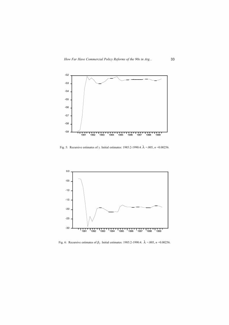
Fig. 5: Recursive estimates of γ. Initial estimates: 1985:2-1990:4. λ =.005, n =0.00256.
Fig. 6: Recursive estimates of β1. Initial estimates: 1985:2-1990:4. λ =.005, n =0.00256.
33How Far Have Commercial Policy Reforms of the 90s in Arg...

Fig. 7: Recursive estimates of β2. Initial estimates: 1985:2-1990:4. λ =.005, n =0.00256.
Fig. 8: Recursive estimates of β3. Initial estimates: 1985:2-1990:4. λ =.005, n =0.00256.
34 Alberto Herrou-Aragón

III. A QUANTITATIVE ASSESSMENT OF THE TRADE POLICIES OF
THE 90S
In this section, the increase in the 1995-1999 average quantity of
imports over the average of 1985-89 is decomposed according to its
sources using the ARCH estimates of the long-run parameters of the
import demand function for the period 1985:3-1999:4 along with the
measures of the equivalent uniform import tax rates for 1985-89 and for
1995-99:
(i) Aggregate expenditure and real output effects holding constant the
average 1985-89 domestic relative prices of importable vis-à-vis
exportable goods and the average external terms of trade for this sub
sample;
(ii) Changes in the external terms of trade holding constant aggregate
expenditure and real output at their 1995:99 levels and the
commercial policies of 1985:89;
(iii) Changes in commercial policies holding constant the external terms
of trade and aggregate expenditure and real output at their average
values of 1995-99.
The results show that the trade liberalization policies of the 90s are
the main factor behind the increase in the volume of imports. The
estimated changes in the equivalent uniform import tax from about 80
percent in the second half of the 80s to about 20 percent in the second half
of the 90s and the estimated price elasticity of the demand for imports of
about -2.00 resulted in an increase in the volume of imports of about 130
percent if the average real expenditure, holding constant real output and
the external terms of trade at their average values of the period 1995-99.
This increase in the quantity of imports is estimated to account for about
68 percent of the actual increase in the total volume of imports10. On the
other hand, changes in real expenditure and in real output account for
about 23 percent of the increase in the volume of imports. The remaining
9 percent is estimated to be accounted for by changes in the external terms
of trade.
35How Far Have Commercial Policy Reforms of the 90s in Arg...
10 The average quantity of imports increased from 29.2 in 1985-89 (1993=100) to 155.5 in 1995-99, representing an increase of about 430 percent.

IV. FINAL REMARKS
According to our estimates, in-depth trade liberalization policies
were implemented during the 90s as indicated by the reduction in the
estimated equivalent uniform tax on international trade of about 60
percentage points compared to the average tax of the period 1985-89. The
equivalent uniform tax rate on the volume of international trade was
reduced from about 80 percent in the second half of the 80s to about 20
percent in the 90s.
The estimates provided in this paper suggest that if the effects of
trade liberalization policies of the 90s are isolated from changes in
aggregate expenditure and in real output, and from changes in external
terms of trade, then, these policies have led to a substantial increase in the
quantity of imports. According to the estimates, the increase in the volume
of imports in response to trade liberalization policies would represent
about 68 percent of the total increase in the volume of imports over the
period of more severe trade restrictions of the late 80s. The remaining 32
percent would be attributed mostly to increases in aggregate expenditure
and real output (23 percent), and to more favorable external terms of trade
(9 percent).
V. REFERENCES
Berlinski, J., “International Trade and Commercial Policies of Argentina”,
Instituto and Universidad Torcuato Di Tella, October 2000.
Díaz-Alejandro, C., Ensayos Sobre la Historia Económica de Argentina,Amorrortu Editores, 1983.
Doan, T., R. Litterman, and C. A. Sims, “Forecasting and Conditional
Projection Using Realistic Prior Distributions”, EconometricReviews, Vol. 3, pp. 1-100,1986.
Harbo, I., S. Johansen, B. Nielsen, and A. Rahbek, “Asymptotic Inference
on Cointegrating Rank in Partial Systems”, Journal of Businessand Economic Statistics, Oct. 1998, 16,4.
Hendry, D. F., Dynamic Econometrics, Oxford University Press 1995.
Sjaastad, L., “La Reforma Arancelaria en Argentina: Implicancias y
Consecuencias”, Agosto 1981, Documentos de Trabajo No 27.
36 Alberto Herrou-Aragón

Urzúa, C. M., “On the correct use of omnibus tests for normality”,
Economics Letters, 53, 1996.
ANNEX A: DATA DESCRIPTION
The volume of import (M) is an index of the quantity of imports
(1993=100). For the period 1993:1-1999:4, the data is from the Institute
of National Statistics and Census (INDEC). Data for data of the periods
1970:1 1999:2 was obtained from national accounts at constant prices.
These data were linked using the rate of change of the quarterly value of
imports at constant prices.
Relative prices of imports are defined as ratio of the
wholesale price index of imports to the price of exports from 1960:1 until
1999:4. Px is a weighted average of the prices of agricultural and food
manufacturing (excluding beverages). The weights of the components of
Px are those of the 1993-1999 wholesale price index, in which prices of
agricultural and food manufacturing receive weights of 47 and 53 percent
respectively. Alternatively, a moving average of the two prices was
constructed using the shares of exports agricultural and manufactures of
agricultural origin in the total of these exports. The results of the
estimation are very robust to changes in the definition of relative prices.
The price ratio is extrapolated backwardly to the year 1939 with the ratio
of the wholesale price of imported commodities to that of agricultural
commodities. For 1935-1939, the wholesale price of non-agricultural
products is used as a proxy for imported commodities.
Real GDP (Y) is the quarterly real gross domestic product at 1993
prices. The same procedure to construct the data of imports is followed.
Real expenditure (Ye) is the quarterly aggregate demand at
constant 1996 prices.
External Terms of Trade data are from Mundlak,Y., D. Cavallo,
and R. Domenech, “Estadísticas de la evolución económica de Argentina:
1913-1984”, Estudios, IX, No 39, Julio-Septiembre 1986. These data are
extrapolated with estimates of the World Bank from 1984 until 1988 and
with INDEC figures afterwards.
37How Far Have Commercial Policy Reforms of the 90s in Arg...

ANNEX B: DERIVATION OF EQUATION (7)
Consider the following autorregressive representation of a variable Y:
Subtracting Yt-1 from both sides of (A1), and adding and
subtracting specific terms, the following equation is obtained:
Rearranging (A2) and collecting terms, the following equations are
obtained:
A generalization of (A4) to more variables is equation (10) in the text.
38 Alberto Herrou-Aragón