NBER WORKING PAPER SERIES

HOW EUROPEAN MARKETS BECAME FREE:A STUDY OF INSTITUTIONAL DRIFT

Germán GutiérrezThomas Philippon

Working Paper 24700http://www.nber.org/papers/w24700

NATIONAL BUREAU OF ECONOMIC RESEARCH1050 Massachusetts Avenue

Cambridge, MA 02138June 2018

We are grateful to Sebnem Kalemli-Ozcan and Carolina Villegas-Sanchez for tremendous help with the ORBIS data; and to Indraneel Chakraborty, Richard Evans and Rüdiger Fahlenbrach for sharing their mapping from the Center for Responsive Politics’ UltOrg to Compustat GVKEYs. We are also grateful to Alberto Alesina, Simcha Barkai, Olivier Blanchard, Sebnem Kalemli- Ozcan, Matthias Kehrig, Luis Cabral, Steve Davis, Janice Eberly, Chad Syverson, Larry White, Harry First, Luigi Zingales, John Haltiwanger, Jean Tirole, Thomas Holmes, Ali Yurukoglu, Jesse Shapiro, Evgenia Passari, Robin Doettling, Jim Poterba and seminar participants at the NBER, the Federal Reserve, University of Chicago, Banque de France, Bundesbank, European Central Bank and New York University for stimulating discussions. We are grateful to the Smith Richardson Foundation for a research grant. The views expressed herein are those of the authors and do not necessarily reflect the views of the National Bureau of Economic Research.

NBER working papers are circulated for discussion and comment purposes. They have not been peer-reviewed or been subject to the review by the NBER Board of Directors that accompanies official NBER publications.

© 2018 by Germán Gutiérrez and Thomas Philippon. All rights reserved. Short sections of text, not to exceed two paragraphs, may be quoted without explicit permission provided that full credit, including © notice, is given to the source.

How European Markets Became Free: A Study of Institutional Drift Germán Gutiérrez and Thomas PhilipponNBER Working Paper No. 24700June 2018, Revised August 2020JEL No. D02,D41,D42,D43,D72,E25,K21,L0

ABSTRACT

Over the past twenty years, Europe has deregulated many industries, protected consumer welfare, and created strongly independent regulators. These policies represent a stark departure from historical traditions in continental Europe. How and why did this turnaround happen? We build a political economy model of market regulation and we compare the design of national and supra-national regulators. We show that countries in a single market willingly promote a supranational regulator that enforces free markets beyond the preferences of any individual country. We test and confirm the predictions of the model. European institutions are indeed more independent and enforce competition more strongly than any individual country ever did. Countries with ex-ante weaker institutions benefit more from the delegation of competition policy to the EU level.

Germán GutiérrezNew York UniversityStern School of Business44 West 4th StreetKMC 9-190New York, NY 10012ggutierr@stern.nyu.edu

Thomas PhilipponNew York UniversityStern School of Business44 West 4th Street, Suite 9-190New York, NY 10012-1126and NBERtphilipp@stern.nyu.edu

If Europe is to arrest its decline [..] it needs to adopt something closer to the American free-

market model. Alesina and Giavazzi (2006)

The United States invented modern antitrust in the late nineteenth and early twentieth century. By 1950

it was clear to most observers that American markets were more competitive that European ones. For

instance, Jean Monnet writes in his Memoirs (published in 1978): “The problem was to break up excessive

concentrations in the coal and steel industries of the Ruhr [..] The Americans had been the first to tackle

the problem, many months earlier. Their economic and political philosophy would not tolerate either the

practice or the apparatus of domination, at home or abroad.” The United States later led the way in the

deregulation of important industries such as Airlines (1978) and Telecoms (1984). The American free-

market doctrine spread globally during the 1980’s and 1990’s, and by the late 1990’s a broad international

consensus had emerged among policy makers in favor of US-style regulations. Alesina and Giavazzi (2006)

perfectly captured this common wisdom of the early 2000s.

We argue that much has changed since then. We show that Europe has heeded the advice of policy mak-

ers and economists. It has set up the world’s most independent antitrust regulator and it has systematically

deregulated many of its markets. In fact, most European markets are now at least as competitive as their

American counter-parts, and several are more competitive. It is well known that US markets experienced a

continuous rise in concentration and profit margins starting in the early 2000s.1 EU markets did not experi-

ence these trends. Figure 1 shows that US profit margins used to be lower than European ones, but a reversal

took place in the mid-2000s. Profit margins in Europe in 2015 are similar to profit margins in the US twenty

years earlier.

Profits and concentration are endogenous variables, however, and need to be interpreted with caution.2

We will present a host of other indicators – including direct comparisons of prices and a detailed study of

product market deregulations – but it is important to clarify that some trends are unambiguous. There is no

doubt that Europe has deregulated many of its markets and that it has improved its antitrust enforcement.

Figure 2 shows the average number of product market reforms implemented by European Countries. Reform

efforts increased significantly in the late 1990s and early 2000s. We are most interested in those reforms

that reduce barriers to entry. Consider for instance the cost of starting a new business. Djankov et al. (2002)

report that it took 53 days to begin operating legally in France in 1999. By 2016, this number was down to

only 4 days. Over the same period, the entry delay in the US went up from 4 days to 6 days. This is not an

isolated indicator. The OECD’s Product Market Regulation indices (discussed later) show clear decreases

in regulations in all EU countries over the past 20 years.

While these policies are relatively easy to document, two key questions have yet to be answered. Why

did Europe break from its historical traditions to move towards free and competitive markets? And did these

policies have real effects? Our paper answers these two questions. We propose a model to explain why

Europe changed its model of market regulation and we test the key predictions of our model. In particular,

1Appendix A provides an extensive review of all the available evidence.2For instance, Covarrubias et al. (2019) explain that concentration and competition are negatively correlated if the data is

generated by entry cost shocks, but positively correlated if the data is generated by shocks to ex-post demand elasticities. Syverson

(2004) provides an example of the later case. Syverson (2019) provides a critical assessment of the recent literature.

2

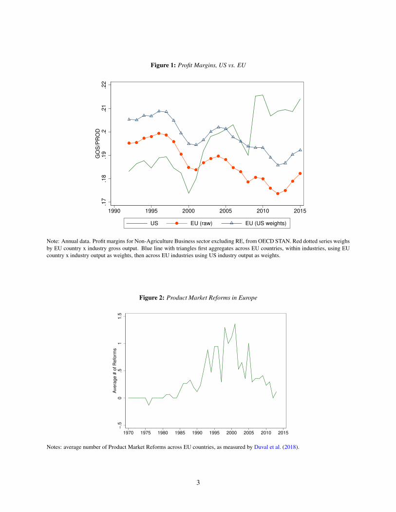
Figure 1: Profit Margins, US vs. EU

.17

.18

.19

.2.2

1.2

2G

OS

/PR

OD

1990 1995 2000 2005 2010 2015

US EU (raw) EU (US weights)

Note: Annual data. Profit margins for Non-Agriculture Business sector excluding RE, from OECD STAN. Red dotted series weighs

by EU country x industry gross output. Blue line with triangles first aggregates across EU countries, within industries, using EU

country x industry output as weights, then across EU industries using US industry output as weights.

Figure 2: Product Market Reforms in Europe

−.5

0.5

11.5

Avera

ge #

of R

efo

rms

1970 1975 1980 1985 1990 1995 2000 2005 2010 2015

Notes: average number of Product Market Reforms across EU countries, as measured by Duval et al. (2018).

3

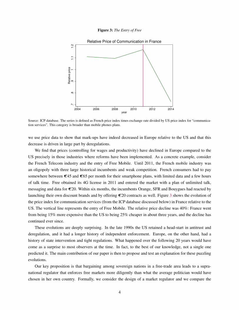
Figure 3: The Entry of Free

.7.8

.91

1.1

1.2

Rela

tive p

rice

2004 2006 2008 2010 2012 2014year

Relative Price of Communication in France

Source: ICP database. The series is defined as French price index times exchange rate divided by US price index for “communica-

tion services”. This category is broader than mobile phones plans.

we use price data to show that mark-ups have indeed decreased in Europe relative to the US and that this

decrease is driven in large part by deregulations.

We find that prices (controlling for wages and productivity) have declined in Europe compared to the

US precisely in those industries where reforms have been implemented. As a concrete example, consider

the French Telecom industry and the entry of Free Mobile. Until 2011, the French mobile industry was

an oligopoly with three large historical incumbents and weak competition. French consumers had to pay

somewhere between C45 and C65 per month for their smartphone plans, with limited data and a few hours

of talk time. Free obtained its 4G license in 2011 and entered the market with a plan of unlimited talk,

messaging and data for C20. Within six months, the incumbents Orange, SFR and Bouygues had reacted by

launching their own discount brands and by offering C20 contracts as well. Figure 3 shows the evolution of

the price index for communication services (from the ICP database discussed below) in France relative to the

US. The vertical line represents the entry of Free Mobile. The relative price decline was 40%: France went

from being 15% more expensive than the US to being 25% cheaper in about three years, and the decline has

continued ever since.

These evolutions are deeply surprising. In the late 1990s the US retained a head-start in antitrust and

deregulation, and it had a longer history of independent enforcement. Europe, on the other hand, had a

history of state intervention and tight regulations. What happened over the following 20 years would have

come as a surprise to most observers at the time. In fact, to the best of our knowledge, not a single one

predicted it. The main contribution of our paper is then to propose and test an explanation for these puzzling

evolutions.

Our key proposition is that bargaining among sovereign nations in a free-trade area leads to a supra-

national regulator that enforces free markets more diligently than what the average politician would have

chosen in her own country. Formally, we consider the design of a market regulator and we compare the

4

equilibrium of the game under two structures: national regulator versus supra-national regulator. Policy

makers design regulators and choose their degrees of independence. Regulators are then subject to lobbying

and political pressures. A fully independent regulator simply maximizes consumer surplus. A less than

fully independent regulator can be swayed ex-post by business lobbies and politicians. We show that the

equilibrium degree of independence is strictly higher when two countries set up a common regulator than

when each country has its own regulator. The key insight is that politicians are more worried about the

regulator being captured by the other country than they are attracted by the opportunity to capture the

regulator themselves. French and German politicians might not like a strong and independent regulator, but

they like even less the idea of the other nation exerting political influence over the regulator. As a result, if

they are to agree on a supra-national regulator, it will be tilted towards more independence.

The strategic value of an independent regulator is even stronger for small countries than for large

ones. The proposed merger of Alstom and Siemens provides a perfect illustration. Germany’s Siemens

and France’s Alstom had decided in 2017 to merge their rail activities. The EU commission was under

strong political pressure from its two largest and influential members to approve the merger. Commissioner

Vestager and her team, however, concluded that the merger “would have significantly reduced competition”

in signaling equipment and high speed trains and decided to block the merger.3 A critical part of the story –

but one that is often forgotten – is that all the other EU countries supported the decision of the commission.

Were it not for a strong and independent EU-level regulator, these countries knew very well they would

have had a hard time blocking the merger. Using backward induction, these countries would have been

reluctant to join a single market without an independent referee. Our model therefore explains why, despite

their historical mistrust of free markets, Europeans deliberately chose to empower a strongly independent

pro-competition regulator at the EU level.

Our model makes several testable predictions: (i) EU countries agree to set up a competition regulator

that is tougher and more independent than their previous national regulators; (ii) This choice has real conse-

quences and leads to more competition in product markets; (iii) Countries with weaker ex-ante institutions

benefit more from delegation to supra-national institutions; and (iv) Independent institutions decrease the

incentives and returns to corporate and political lobbying.

We test these predictions in the remainder of the paper. One plausible theory of European integration is

that EU institutions should reflect the (weighted) average of member states’ institutions. Our theory makes

a sharply different prediction. Our model predicts that EU institutions will protect free markets more than

any member states. This prediction applies to market regulations in general. Among the examples discussed

above, one was a regulatory decision (the entry of Free), the other was an antitrust decision (blocking the

merger of Alstom and Siemens). We study both in our empirical analysis. We start with antitrust – merger

and non-merger reviews and remedies – because it has clearly become an EU-level competency in the case of

large mergers. Using indicators of competition law and policy from the OECD and from Hylton and Deng

(2007), we show that DG Comp is indeed more independent and more pro-competition than any of the

national regulators. In fact, it is more independent that its US counterparts. Consistent with this institutional

fact, we show that enforcement has remained stable (or even tightened) in Europe while it has become laxer

3EU Commission, press release of February 6, 2019.

5

in the US.

We then study product market regulations, which is usually a shared competency between the member

state and the EU (see below for details). Once again, we find that the EU has become relatively more

pro-competition than the US over the past 15 years. Product market regulations and barriers to entry have

decreased in Europe, while they have remained stable or increased in the US.

Using data across industries and across countries, we then show that these reforms have had real effects.

Markups have fallen in Europe relative to the US, and differential enforcement and product market reforms

explain the relative declines across time, countries and industries.

Next, we show that EU countries with initially weak institutions have experienced large improvements

in antitrust and product market regulation. Moreover, we find that the relative improvement is larger for

EU countries than for non-EU countries with similar initial institutions. For instance, in 1998, Poland

had the same level of entry barriers as Turkey; Portugal and the Czech Republic the same as Mexico.

Fifteen years later, as predicted by our model, EU countries have experienced much larger improvements

in product market regulations than their non-EU peers. Finally, moving to political expenditures, we show

that European firms spend substantially less on lobbying and campaign contributions, and that they are less

likely to succeed than American firms/lobbyists.

Literature. Our paper is related to several strands of literature. We discuss only key references here,

and provide more detailed discussions throughout the paper. Grullon et al. (2019) show that concentra-

tion and profit rates have increased across most US industries, and Barkai (2017) estimates profits in ex-

cess of required returns on capital. Furman (2015) and CEA (2016) argue that the rise in concentration

suggests “economic rents and barriers to competition” but Shapiro (2018) and Werden and Froeb (2018)

criticize the use of concentration measures based on SIC or NAICS. Autor et al. (2017) show that the in-

crease in concentration is linked to the decrease in the labor share. Gutiérrez and Philippon (2017a) and

Jones et al. (2019) argue that declining competition explains part of the weakness of corporate investment

while Crouzet and Eberly (2018a) emphasize the role of intangible investment. De-Loecker et al. (2019)

and Hall (2018) provide estimates of markups in the US.

There is much controversy about the interpretation of these trends, particularly as they relate to compe-

tition policy. Kwoka (2015) criticizes the weakening of merger reviews in the US over the past 20 years.

Vita and Osinski (2016) offer a rebuttal while Kwoka (2017a) maintains the validity of his original claim.

Bergman et al. (2010) find that the EU has been tougher than the US in its review of dominance mergers – at

least up to 2004. Bailey and Thomas (2015) find a negative correlation between regulation and measures of

business dynamism and Davis (2017) argues that excessive regulations have increased barriers to entry in the

US. Faccio and Zingales (2017) show that political factors and regulations explain much of the variations

in the price of mobile telecommunication around the world. Besley et al. (2020) show that profit margins

of firms operating in non-tradable sectors are significantly lower in countries presenting stronger anti-trust

policies compared to firms operating in tradable sectors.

Our paper also contributes to the literature on the political economy of institutions. A classic idea

from monetary economics is that rules dominate discretion when optimal policies are time-inconsistent

6

(Kydland and Prescott, 1977; Calvo, 1978). Reputation can sustain some rules (Barro and Gordon, 1983)

but external commitments can be necessary, such as a conservative policy marker (Rogoff, 1985) or a cur-

rency board. Debrun (2001) develops the twin sister argument for the ECB vis a vis the Bundesbank.

Faure-Grimaud and Martimort (2003) and Faure-Grimaud and Martimort (2007) argue that regulatory inde-

pendence can insulate policies from political cycles.4 Rajan and Zingales (2003) emphasize the role of free

financial markets in maintaining a level playing field for competition and innovation. Jabko (2012) shows

that the single market was a deliberate political construction and not the by-product of some inevitable

process of globalization. More broadly, our paper sheds light on the economic analysis of institutions, pio-

neered by North (1990) and discussed by Acemoglu et al. (2005). We show how effective enforcement and

regulations can drift over time even in the absence of explicit institutional change.

The remainder of this paper is organized as follows. Section 1 presents our model of regulatory inde-

pendence and its testable predictions. Section 2 documents the rise of regulatory independence and tougher

enforcement of free markets. Section 3 documents the decline in markups and shows that it is explained

by policy changes. Section 4.1 tests the cross-sectional and political economy implications of the model.

Section 5 concludes. The Appendix provides additional results and discussion for each section, along with

a detailed description of the data and process to replicate the results.

1 Model

We present a model of the design of EU institutions. There are two goods, two periods, and either one or

two countries. In the first period policy makers designs the regulator. In the second period, the regulator

protects consumer welfare but is subject to lobbying pressures. We interpret the first period as the 1980’s

and 1990’s, when EU institutions are designed, and the second period as the 2000’s when we observe the

evolution of Europe relative to the US. We solve the model by backward induction, first with one country,

then with two countries under free trade.

4Faure-Grimaud and Martimort (2007) explains that “the European Central Bank remains the most spectacular example of

delegation to a new European institution,” but the EU “has also created a dozen of independent agencies over the last thirty years

or so [..] For instance, in the field of merger control, the European Commission was delegated the competence to regulate mergers

under the 1989 Merger Control Regulation.” The role of economists within the DG comp has increased during the 2000’s, in

particular with the creation of the position of Chief Competition Economist in 2003. The position EU commissioner for competition

is prestigious, attracts high caliber politicians, and benefits from strong public recognition.

7

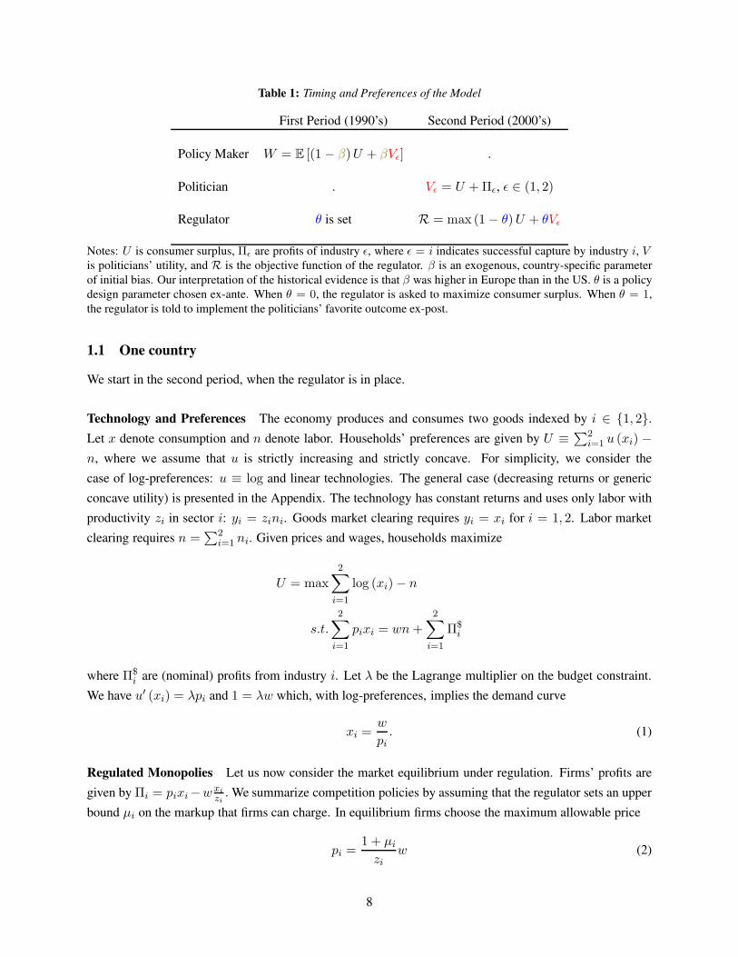
Table 1: Timing and Preferences of the Model

First Period (1990’s) Second Period (2000’s)

Policy Maker W = E [(1− β)U + βVǫ] .

Politician . Vǫ = U +Πǫ, ǫ ∈ (1, 2)

Regulator θ is set R = max (1− θ)U + θVǫ

Notes: U is consumer surplus, Πǫ are profits of industry ǫ, where ǫ = i indicates successful capture by industry i, Vis politicians’ utility, and R is the objective function of the regulator. β is an exogenous, country-specific parameter

of initial bias. Our interpretation of the historical evidence is that β was higher in Europe than in the US. θ is a policy

design parameter chosen ex-ante. When θ = 0, the regulator is asked to maximize consumer surplus. When θ = 1,

the regulator is told to implement the politicians’ favorite outcome ex-post.

1.1 One country

We start in the second period, when the regulator is in place.

Technology and Preferences The economy produces and consumes two goods indexed by i ∈ {1, 2}.

Let x denote consumption and n denote labor. Households’ preferences are given by U ≡ ∑2i=1 u (xi) −

n, where we assume that u is strictly increasing and strictly concave. For simplicity, we consider the

case of log-preferences: u ≡ log and linear technologies. The general case (decreasing returns or generic

concave utility) is presented in the Appendix. The technology has constant returns and uses only labor with

productivity zi in sector i: yi = zini. Goods market clearing requires yi = xi for i = 1, 2. Labor market

clearing requires n =∑2

i=1 ni. Given prices and wages, households maximize

U = max

2∑

i=1

log (xi)− n

s.t.2∑

i=1

pixi = wn+2∑

i=1

Π$i

where Π$i are (nominal) profits from industry i. Let λ be the Lagrange multiplier on the budget constraint.

We have u′ (xi) = λpi and 1 = λw which, with log-preferences, implies the demand curve

xi =w

pi. (1)

Regulated Monopolies Let us now consider the market equilibrium under regulation. Firms’ profits are

given by Πi = pixi−w xi

zi. We summarize competition policies by assuming that the regulator sets an upper

bound µi on the markup that firms can charge. In equilibrium firms choose the maximum allowable price

pi =1 + µi

ziw (2)

8

Using equations (1) and (2), we then get the equilibrium output

xi =zi

1 + µi

There is a direct mapping between the markup and the quantity produced in equilibrium. We can therefore

think of the regulator as indirectly choosing the quantities {xi}i=1,2. This leads to the indirect utility function

for the households

U ({xi}i) =2∑

i=1

log (xi)−xizi.

Nominal profits can be written as a function of markups or quantities Π$i = wµi

xi

zi= w µi

1+µi= w

(

1− xi

zi

)

.

We define real profits as Πi = Π$i /w and therefore

Πi = 1− xizi

Note that ∂π∂xi

< 0 and that the consumer welfare maximizing level is x∗i = zi, which corresponds to µi = 0

and Πi = 0. The first best utility level is

U∗ =2∑

i=1

log (zi)− 2.

Welfare and Capture Ex-Post Firms seek to influence politicians and regulators in order to increase their

market power. It is important in our model to distinguish regulators from politicians because the preferences

of the regulators are endogenous. Formally, then, we assume that firms seek to capture politicians who can

then exert influence on regulators. Note, however, that in the one country case this model is isomorphic to

one where firms influence regulators directly.

As in the political support literature, we assume that politicians’ utility is a mixture of social welfare and

corporate profits, and we consider random capture by one of the two industries. The utility of politicians is

V (ǫ) = U +Πǫ,

where ǫ = 1, 2 with equal probability.5 Our specification of the utility function is similar to the one in

Grossman and Helpman (1994). The main difference is that we assume that politicians affect market out-

comes by influencing regulators. Regulators are subject to political pressure. They maximize a weighted

average of consumers welfare U and politicians’ utility V

R (ǫ) = max{µi}

(1− θ)U + θV (ǫ) (3)

The parameter θ captures the degree of influence of politicians over regulators. It is set in the first period and

taken as given in the second period. The point of our model is to understand the forces that determine θ and

5The Appendix considers utilities of the form U + γΠǫ where γ is an ex-post political capture parameter. As long as γ is not

random the simple formulation above is without loss of generality.

9

how they change when we consider a supra-national regulator. Throughout our discussion, we think of the

institutional design of θ as encompassing all competition policy, from entry and product market regulation,

to antitrust, to judicial review.

For simplicity, but with a slight abuse of notations, we write xi=ǫ ≡ xi (ǫ = i) for the output of the

industry that captures the politicians, and xi 6=ǫ ≡ xi (ǫ 6= i) for the other one. We measure the deviation

from ex-post consumer surplus maximization by the variable m defined as the ratio of output to efficient

output:

mi ≡xix∗i

,

and recall that with constant returns and log-preferences we simply have x∗i = zi. We will use m to denote

the equilibrium with one country and ms to denote the equilibrium with a supra-national regulator. We have

the following Lemma.

Lemma 1. In the one country model with random capture, one industry is competitive (xi 6=ǫ = zi and

Πi 6=ǫ = 0) while the other industry charges a markup γθ: xi=ǫ = mzi and Πi=ǫ = 1− m where m ≡ 11+γθ .

The ex-post utility of the representative household is

U (θ) = U∗ + log (m) + 1− m.

Proof. The program of the regulator is equivalent to

max{xi}

U ({xi}i) + θΠǫ

We can write the objective function as

2∑

i=1

log (xi)−xizi

+ 1i=ǫθ

(

1− xizi

)

The solution is xi 6=ǫ = zi and xi=ǫ =zi1+θ , so m = 1

1+θ .

Ex-Ante Design of Regulatory Independence The first period corresponds to the design of institutions.

In the case of national regulators we think of the design that existed before the single market. In the case of

Europe, we think of politicians and civil servants setting up the framework for EU competition policy in the

1990’s. The utility of the politicians building the regulatory framework is

W = E [(1− β)U + βVǫ]

The founding fathers choose θ to maximize W .

Lemma 2. In a closed economy (one country), the politicians choose a regulatory framework with influence

parameter

θ = β

10

There are several ways to interpret the parameter β. In the equations above, β captures the bias in the

preferences of the politicians designing the institutions. In our simplified setup a benevolent planner would

create fully independent institutions charged simply with maximizing consumer surplus. In reality, there

might be legitimate reasons to deviate from strict consumer surplus maximization: externalities, entry costs,

innovations, etc. In Lim and Yurukoglu (2018), for instance, there is an optimal ex-post return on capital

that encourages efficient investment ex-ante. The appendix presents a simple model where a benevolent

planner chooses θ, taking into account externalities.6

Perhaps more importantly, there are significant ideological differences among politicians. Lim and Yurukoglu

(2018) find that “conservative regulators [within the US] mitigate welfare losses due to time inconsistency,

but worsen losses from moral hazard.” There are also persistent differences across countries. In France, there

is a long tradition of “Colbertisme”, which argues for state intervention in the economy and for industrial

policy aimed at protecting firms from excessive competition. Historically, the UK, and later the US, have

championed a more free-market approach, and have been suspicious of politicians exerting direct influence

on business decisions. These stereotypes are somewhat simplistic but they capture material differences in

how countries operate. We can thus also think of France or Italy as being high β countries for ideological

reasons.

1.2 Supra-National Regulatory Design

We now extend our model to two countries and we assume that production is specialized. Technology and

preferences are identical to the one country case. The only difference is that politicians choose a single

regulator for the free trade area.

Country i produces good i. We assume that the law of one price holds, so that the price of good i is

the same in both countries. Let xi,j denote the consumption of good j in country i. Consumer welfare in

country i is given by

Ui =

2∑

j=1

log (xi,j)− ni.

The demand for goods is similar to equation (1) except that wages might differ across countries: xi,j =wi

pj.

Balanced trade requires

p1x2,1 = p2x1,2

This implies w1 = w2.7 Given that wages and prices are equalized, so are the quantities consumed for each

good: xi,i = xi,j ≡ xi. Since pi = (1 + µi)wi/zi, we still have xi = zi1+µi

. Market clearing requires

6A good example is that of technological clusters. One can view them as places where innovative individual and businesses can

come together and shares ideas. Clusters generate plausible externalities that can justify political interventions. On the other hand,

they are “absolute catnip for policy makers and pundits” as Haskel and Westlake (2017) argue. All we need for the benevolent

interpretation of our model is that there is a legitimate case of externality, yet politicians cannot be fully trusted.7This is the simplification brought by assuming log preferences. When the demand elasticity is not one, then the relative wage

will in general differ from one. This does not change our main results but it complicates the exposition.

11

zini = xi,i + x−i,i = 2xi, so in equilibrium, we have

Ui = log (xi) + log (xj)−2xizi

(4)

and profits are

Πi = 2

(

1− xizi

)

Ex-Post Regulatory Capture Politicians care about domestic consumer welfare and about the profits

of domestic industries: Vi = Ui + Πi. Politicians from each country attempt to influence the common

regulator and are equally likely to succeed. Let ǫ denote the winning country. The supra-national regulator

then maximizes (1− θ) (U1 + U2) + θVǫ, which we can also write as

Rs (ǫ) = maxUi=ǫ + (1− θ)Ui 6=ǫ + θΠi=ǫ.

Using (4), the objective function becomes (2− θ) log (xi=ǫ)+(2− θ) log (xi 6=ǫ)−(1 + θ) 2xi=ǫ

zi=ǫ−(1− θ)

2xi6=ǫ

zi6=ǫ+

2θ. Let “s” to denote the equilibrium with a supra-national regulator. The solution is

xǫ=i

zi= ms (θ) ≡ 1− θ

2

1 + θ< m,

xǫ 6=i

zi= M s (θ) ≡ 1− θ

2

1− θ> 1.

The allocation is distorted in two ways compared to the one country model. First, politicians perceive a

different trade-off between profits and welfare because higher prices fall partly on foreign households. This

explains why ms < m. Second, they seek to impose lower markups to foreign producers in order to benefit

domestic households.8 This explains why M s > 1. The risk of “regulatory over-reach”, as emphasized by

the Chicago school, is higher than in the one country case. Ex-post utilities are

Ui=ǫ = U∗ + log (ms) + log (M s) + 2 (1−ms)

Ui 6=ǫ = U∗ + log (ms) + log (M s) + 2 (1−M s)

Ex-Ante Design Let us consider the choice of θ. The expected utility of policy makers from country i

under supra-national supervision is

W s (θ) = E [(1− β)Ui + βVi] = E [Ui + βΠi]

= U∗ + log (ms) + log (M s) + (1 + β) (2−ms −M s)

8With linear technologies this implies negative operating profits. It is easy to extend the model to include decreasing returns

and fixed entry costs. In that case operating profits would be still positive, as shown in the Appendix.

12

This new program differs from the one country program in two ways. First, ms (θ) implies a different

mapping than m (θ). This means that, even if we ignored M s, implementing the preferred markup β would

require a lower value of θ.9 Second, increasing θ lowers ms but it increases M s. This implies more

independence and lower average markups. The following proposition summarizes our results.

Proposition 1. Politicians choose a higher degree of independence for a supra-national regulator than for

a national one:

θs ∈ (0, β) .

Since M ′ (θ) > 0, the equilibrium also implies more competitive markets ex-post: ms (θs) > m (β).

Proof. M is a strictly increasing function of θ while m is decreasing in θ. The objective function is

W s (θ)− U∗ = log (m) + log (M) + (1 + β) (2−m−M)

The derivative is

∂W s

∂θ=

m′

m+

M ′

M− (1 + β)

(

m′ +M ′)

= −m′(

1 + β +

(

1 + β − 1

M

)

M

m′

′− 1

m

)

Therefore the solution is1

m= 1 + β +

M ′

m′

(

1 + β − 1

M

)

Since M > 1, M ′ > 0 and m′ < 0 we have M ′

m′

(

1 + β − 1M

)

< 0 and therefore m is larger than (1 + β)−1.

This proves ms (θs) > m (β) if and only if M ′ > 0. Since ms < m for all θ, this also proves θs < β. Next

we need to show that θs > 0. When θ = 0 and m = M = 1, we have ∂M∂θ = 1

2 ; ∂m∂θ = −32 therefore

M ′

m′ (0) = −1

3

Thus

1 + β + βM ′

m′ (0) = 1 +2

3β > 1

and therefore∂W

∂θ(0) > 0

Starting from θ = 0, a marginal increase in markups raises the ex-ante value function of politicians. This

proves θs > 0. QED.

Proposition 1 contains the first two predictions of our theory: (i) EU countries should design a supra-

national regulator that is more independent than pre-existing national regulators; and (ii) this will lead to

stronger protection of consumer welfare in equilibrium. Our theory predicts that the supra-national regulator

9To achieve a markup of γβ, i.e., to get the quantity m = 1

1+βγ, the designer would need to set θ = βγ

γ+1+βγ

2

.

13

should not reflect the average of countries’ preferences, but instead, we should observe a discrete increase

in independence and a stricter enforcement of competition. The key insight comes from comparing the

consequences of potential regulatory capture. The capture of a joint regulator leads to larger welfare losses

because national politicians do not care about the citizens of other countries. As a result, it is efficient to

commit ex-ante to a more independent regulator. This, in our view, explains why DG Comp is structurally

more insulated from political and lobbying pressures than national regulators used to be.10

The second prediction might seem obvious but it is not. If M ′ = 0 we would have ms (θs) = m (β)

even though θs < β. Countries would choose a different θ to achieve the same average m. The fact

that ms (θs) > m (β) reflects the extra risk created by the capture of a supra-national regulator. In fact,

the simple model above hides another source of risk because agents with linear disutility of labor and linear

technology can fully smooth consumption by adjusting their labor supply. The Appendix derives the solution

under a concave production frontier. There is then an additional argument for independence of the supra-

national regulator because gains and losses are asymmetric.

1.3 Extensions

We now extend the basic model to obtain other predictions regarding lobbying and ex-ante heterogeneity

across countries. It is straightforward to extend our analysis to the case of N countries. We show in the

Appendix that regulatory independence increases with N and converges to a finite value as N becomes

large.

Heterogeneous Countries Some of our empirical tests relate to ex-ante heterogeneity among countries.

For instance, we show that EU countries with weaker ex-ante institutions benefit more from supra-national

regulation. Consider two countries such that β1 < β2. Before integration, country 2 has more biased

politicians, more captured regulators, and weaker competition. We know that

W si (θ)− U∗ = log (ms (θ)) + log (M s (θ)) + (1 + βi) (2−ms (θ)−M s (θ))

Assuming equal bargaining power at the design stage we solve

maxθ

2∑

i=1

W si (θ)

The first order condition ism′

m+

M

M

′−(

1 +β1 + β2

2

)

(

m′ +M ′)

We then have the following straightforward proposition.

Proposition 2. Countries with weaker ex-ante institutions benefit more from supra-national regulation.

10Interestingly, this does not imply a complete lack of democratic accountability as evidenced by the evolution of DG Comp

from an entirely independent organization to an increasingly democratic one following the 2004 reforms (First and Weber Waller,

2013).

14

Countries with low initial β benefit less, but because the average β goes down, they still benefit as long

as the distribution of β’s is not too wide. Also notice that we have followed a weighted average approach at

the design stage. In reality the EU Commission explicitly promotes best practice and we can expect low β

countries to have more sway.

Lobbying Introducing lobbying explicitly allows us to make another testable prediction. Suppose firms

spend l real resources on lobbying – they hire l lobbyists for instance.11 We assume that the influence of

lobbyists is measured by the function Γ (l; θ), increasing in both arguments and super modular. Equation

(3) then becomes

R = max{x}

U (x) + Γ (l; θ)Π

We know that this leads to m ≡ 11+Γ and Π = Γ

1+Γw. For simplicity we consider here the one-country

model, but it is straightforward to derive similar results with many countries. Firms maximize profits net of

lobbying expenses Π$i = pixi − w xi

zi− wl. This is equivalent to

max{l}

Γ (l; θ)

1 + Γ (l; θ)− l

From the super-modularity of Γ (l; θ), it is clear that the solution l (θ) is an increasing function. We then

have the following proposition.

Proposition 3. In countries with more independent regulators, lobbyists are less successful and firms spend

less on lobbying.

An example of a simple functional form is Γ (l; θ) =√γlθ

1−√γlθ

. In that caseΓ(l;θ)

1+Γ(l;θ) =√γlθ and therefore

l (θ) = γθ4 and, in equilibrium, Γ (θ) = γθ

2−γθ , which is a simple renormalization of the formula that we have

used so far. We will discuss in Section 4.2 how shocks to lobbying can also help us understand the divergence

between the US and Europe.

Choosing a Single Regulator So far we have taken as given the existence of a single regulator. But would

politicians actually prefer to retain national regulators in the context of the single market? Let us consider

what the equilibrium would be under free trade but without joint supervision. The regulator in country i

would solve

maxxi

Ui + θiΠi = log (xi) + log (x−i)− 2xizi

+ 2θi

(

1− xizi

)

which leads to xi =12

zi1+θi

and profits Πi = 2(

1− xi

zi

)

. Note that the allocation is distorted even without

direct influence because the country acts as a monopolist. The ex-ante value for the politicians is Wi =

Ui + βiΠi. They would choose θi = βi as in the one country case. This would implement xi =12

zi1+θi

and

11Official lobbying and corruption are clearly different, both legally and empirically, but that distinction does not really matter

in our model. One can think of l as the number of lawyers and consultants hired, as campaign contributions, or as bribes. In our

empirical analysis, however, we will measure “legal” lobbying.

15

deliver ex-ante utility

Wi = U∗ + 1− 2 log 2− log (1 + βi)− log (1 + βj) + 2βi.

Recall that with supra-national regulation we have W s = U∗+log (msθ)+log (M s

θ )+(1 + βi) (2−msθ −M s

θ ),

for the optimally chosen θ = θs and the implied ms (θs) and M s (θs). We can show the following proposi-

tion

Proposition 4. There exists an upper bound β on political bias such that, if β < β, all politicians agree to

set up a common regulator as described in Proposition 1.

Proof. Politicians prefer a supra-national regulator as long as W s > Wi. We have

W s −Wi = 2 log 2− 1 + log (msθ) + log (M s

θ )

+ (1 + βi) (2−msθ −M s

θ ) + log (1 + βi) + log (1 + β−i)− 2βi

When βi = β−i = 0, we have m = M = 1 and W s −Wi = 2 log 2− 1 > 0. By continuity this extends to

values of β that are strictly positive. On the other hand, if β is large, we can have W s −Wi < 0.

This proposition is reminiscent of others in political economy that a union is feasible when heterogeneity

across its members is not too large.

1.4 Summary of Model Predictions

The model yields the following key predictions

1. Proposition 1 (a): EU countries agree to set up a competition regulator that is tougher and more

independent than their old national regulators.

2. Proposition 1 (b): The implementation of the single market leads to real increases in product market

competition.

3. Proposition 2: Countries with weaker ex-ante institutions benefit more from delegation to supra-

national institutions.

4. Proposition 3: Lobbying is lower when regulators are more independent.

We test these predictions in the rest of the paper. The data appendix describes our data, compiled from a

variety of sources. We focus on two important determinants of competition: antitrust and product market

regulation. Both of these were developed with, and played a critical role in the creation of the Single Market.

Antitrust was established as a supra-national capability at the time of creation of the Single Market: Article

3(1)(g) of the 1957 Treaty of Rome envisioned “a system ensuring that competition in the internal market

16

is not distorted”.12 Product market reforms came later. They started on a limited scope with the 1985

Single Market Plan, and accelerated in the 2000s with the Lisbon Strategy, which aimed “at opening up

product markets to competition in particular by completing the internal market for goods and services, by

removing obstacles to competition in Member States and by creating a business environment more conducive

to market entry and exit”(Zeitz, 2009). While the Lisbon Strategy failed in some dimensions, substantial

product market reforms were implemented.13

2 Test of Proposition 1(a): Tougher and more independent regulator

Proposition 1 implies that a joint regulator is more likely to be a tough regulator. Empirically, we can break

down this prediction into three components. The first is the design of the antitrust regulator, i.e., the formal

framework defining the potential actions of the regulator, which is called “Laws & Policy”. To make this

comparison, we can rely on extensive existing research. The key prediction of our theory is that we should

observe a discrete difference between the EU national regulators and the EU’s supra-national one. The

second prediction concerns enforcement actions by the regulator. This comparison is more complicated and

the data are noisier but the results are consistent. The third prediction relates to Product Market Regulation.

The EU has only partial oversight over Member States’ regulations – but supranational institutions still play

a role. The EU can formally influence regulations in three ways: it can directly prohibit certain domestic

regulations (e.g., prohibition of price controls in transportation industries); it can work with member states to

achieve mutual recognition of restrictions; or it can enact case law based on a treaty (e.g., ongoing regulation

of State Aid by DG Comp). The EU also exerts informal influence using benchmarking, disclosure and peer

pressure.14

12See Appendix F for a brief history of Antitrust institutions on both sides of the Atlantic. The first of US institutions were

established with the The Sherman Act of 1890. The foundations of European competition policies were established much later – in

the 1957 Treaty of Rome, which built on the European Coal and Steel Community (ECSC) of 1951. Council Regulation 17 made

the enforcement powers effective in 1962, and the EU Commission made its first decision in 1964. This regulation was modernized

by regulation 1/2003, which has been effective since May 2004.13Some countries (such as the UK) pursued economic deregulation independently as early as 1979. Why did European economic

integration happen so quickly in the 1980s and 1990s? The answer is far from obvious. The single market was not the by-product

of some inevitable process of globalization. An astute observer in 1980 could not easily have predicted the rapid emergence of

the Single Market. Jabko (2012) argues that the European Commission played to its advantage the idea of the ‘market’ in order

to promote European integration. Jabko’s demonstration relies on four detailed case studies: the integration of financial markets,

the deregulation of the energy market, structural policies (such as development policies for new member states), and the European

Monetary Union (EMU). In all these cases, Jabko argues that the Commission used the idea of the ‘market’ to promote its agenda

of European integration. This idea, however, meant different things to different people. Depending on the audience, it was possible

to emphasize the free-market component, the common regulation, or the protection from the economic giants of Asia and America.14During the implementation of the Lisbon Strategy, for example, the overall objectives were set jointly by the EU and Member

States. From then on, Member States were in charge of implementation but were also required to submit reports to the European

Commission on an on-going basis: the so-called Cardiff Reports from 200-2004, followed by National Reform Programs and

implementation reports. The EU used those reports to continuously monitor and disclose progress – including the creation of the

Microeconomic Reform database (MICREF) which compiled and tracked progress across all states. EU and peer pressure were seen

as key ‘embarrassment tools’ available to encourage reform. If countries still fail to implement required reforms, the Commission

may curtail the allocation of the EU Cohesion Funds. Last, for states in the process of accession, stringent reform requirements

are negotiated in advance – as evidenced by the substantial reforms implemented at new EU Member States in Central and Eastern

Europe.

17

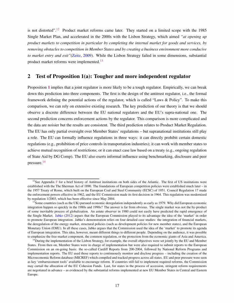
2.1 Design

Let us start with regulatory design. Figure 4 shows the indicators of Competition Law & Policy published by

the OECD in 2013 (Alemani et al., 2013). A lower value signifies better regulation. Indicators are available

for each country’s National Competition Authority (NCA) as well as DG Comp. In Europe, NCAs deal with

cases that have national impact. The European Commissioner for Competition and the Directorate-General

for Competition (DG Comp) enforce European competition law in cooperation with the NCAs. DG Comp

prepares decisions in three broad areas: antitrust, mergers, and state aid.

Consistent with the predictions of our model, DG Comp is more independent and more pro-competition

than any of the national regulators. DG Comp attains the best possible score in the three categories that

directly map into our model: Scope of Action, Policy on Anticompetitiveness, and Probity of Investigation.15

Probity of Investigation measures government interference in antitrust policy. For instance, it measures

whether governments can interfere with the investigations or the decisions taken on antitrust infringements

and mergers. DG Comp is essentially free from interference by national governments and its score is much

lower than the average score of national authorities. Another striking feature of the data is that DG Comp

scores better than American regulators. Historically, it is clear that θUS = βUS < βEU , where βEU would

be the “average” across EU countries. On the other hand, Proposition 1 says that θEU < βEU . Our model

can explain θEU < θUS as long as the costs of potential distortions in the single market are large enough.

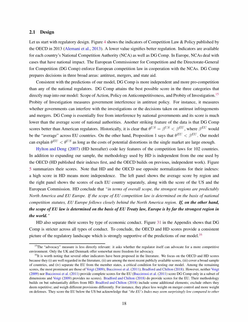
Hylton and Deng (2007) (HD hereafter) code key features of the competition laws for 102 countries.

In addition to expanding our sample, the methodology used by HD is independent from the one used by

the OECD (HD published their indexes first, and the OECD builds on previous, independent work). Figure

5 summarizes their scores. Note that HD and the OECD use opposite normalizations for their indexes:

a high score in HD means more independence. The left panel shows the average score by region and

the right panel shows the scores of each EU country separately, along with the score of the US and the

European Commission. HD conclude that “in terms of overall scope, the strongest regions are predictably

North America and EU Europe. If the scope of EU competition law is determined on the basis of national

competition statutes, EU Europe follows closely behind the North America region. If, on the other hand,

the scope of EU law is determined on the basis of EU Treaty law, Europe is by far the strongest region in

the world.”

HD also separate their scores by type of economic conduct. Figure 31 in the Appendix shows that DG

Comp is stricter across all types of conduct. To conclude, the OECD and HD scores provide a consistent

picture of the regulatory landscape which is strongly supportive of the predictions of our model.16

15The “advocacy” measure is less directly relevant: it asks whether the regulator itself can advocate for a more competitive

environment. Only the UK and Denmark offer somewhat more freedom for advocacy.16It is worth noting that several other indicators have been proposed in the literature. We focus on the OECD and HD scores

because they (i) are well regarded in the literature, (ii) are among the most recent publicly available scores, (iii) cover a broad sample

of countries, and (iv) separate the EU from the member states, a critical condition for testing our model. Among the remaining

scores, the most prominent are those of Voigt (2009); Buccirossi et al. (2011); Bradford and Chilton (2018). However, neither Voigt

(2009) nor Buccirossi et al. (2011) provide complete scores for the EU (Buccirossi et al. (2011) score DG Comp only in a subset of

dimensions and Voigt (2009) provides no scores). Bradford and Chilton (2018) do provide scores for the EU. Their methodology

builds on but substantially differs from HD. Bradford and Chilton (2018) include some additional elements; exclude others they

deem repetitive; and weigh different provisions differently. For instance, they place less weight on merger control and more weight

on defenses. They score the EU below the US but acknowledge that “the EU’s Index may seem surprisingly low compared to other

18

Figure 4: Restrictions on Competition Law & Policy (OECD Indicators, 2013)

DG Comp

−.5

0.5

11

.52

AU

SA

UT

BE

LB

GR

CA

NC

HE

CZ

ED

EU

DN

KE

SP

ES

TF

INF

RA

GB

RG

RC

HU

NIR

LIT

AJP

NK

OR

LT

UL

UX

LV

AM

LT

NL

DN

OR

PO

LP

RT

RO

US

VK

SV

NS

WE

US

A

Scope of Action

DG Comp

−.5

0.5

11

.52

AU

SA

UT

BE

LB

GR

CA

NC

HE

CZ

ED

EU

DN

KE

SP

ES

TF

INF

RA

GB

RG

RC

HU

NIR

LIT

AJP

NK

OR

LT

UL

UX

LV

AM

LT

NL

DN

OR

PO

LP

RT

RO

US

VK

SV

NS

WE

US

A

Policy on Anticompetitiveness

DG Comp

−.5

0.5

11

.52

AU

SA

UT

BE

LB

GR

CA

NC

HE

CZ

ED

EU

DN

KE

SP

ES

TF

INF

RA

GB

RG

RC

HU

NIR

LIT

AJP

NK

OR

LT

UL

UX

LV

AM

LT

NL

DN

OR

PO

LP

RT

RO

US

VK

SV

NS

WE

US

A

Probity of Investigation

DG Comp−

.5.5

1.5

2.5

AU

SA

UT

BE

LB

GR

CA

NC

HE

CZ

ED

EU

DN

KE

SP

ES

TF

INF

RA

GB

RG

RC

HU

NIR

LIT

AJP

NK

OR

LT

UL

UX

LV

AM

LT

NL

DN

OR

PO

LP

RT

RO

US

VK

SV

NS

WE

US

A

Advocacy

Note: higher bar means more restrictions (less pro-competition enforcement). Sample includes EU countries plus AUS, CAN,

JPN, KOR, NOR, CHE and USA. Here are a few examples of each category: Are there exemptions from the competition law for

public and foreign firms (scope of action)? Are anticompetitive behaviors and anticompetitive mergers prohibited? Have there been

interventions recently against such behaviors (policy on anticompetitiveness)? Do governments interfere with the investigations

or the decisions taken on antitrust infringements and mergers (probity of investigation)? Can regulators advocate for a more

competitive environment, e.g., by performing market studies and delivering recommendations (advocacy)? Source: Alemani et al.

(2013).

Figure 5: Hylton and Deng Antitrust Indicators: Overall

01

02

03

0

sout

h_am

erica

cent

ral_am

erica

afric

a

middle_

east

carib

bean

asia

ocea

nia

non_

eu

eu_n

cas

north

_am

erica

dg_c

omp

By Region (Global)

01

02

03

0

LUXCYP

AUTDEU

FINGRCSVK

BELBG

RCZE

IRLM

LTPR

TEST

LTULV

ASVN

SWEDNKGBR

ITANLD

POLROUUSA

HUNESP

FRA

EU

By Country (EU and US only)

Notes: higher bar means stronger competition law. Left plot shows the average total Antitrust “scope index” by region, as reported

in Hylton and Deng (2007). EU NCAs measures the average score of member state’s Competition laws before integration

with EU law. Right plot shows the most recent score of individual countries, as well as those of DG Comp. Individual country

scores may have been updated since publication of Hylton and Deng (2007), so we gather them manually from link.

19

2.2 Enforcement

Do tougher policies translate into tougher enforcement? To shed light on this question we study recent

trends in merger and non-merger enforcement. This is a difficult endeavor because regulatory actions are an

equilibrium outcome influenced by many factors, including expectations of market participants, and because

actions are not necessarily defined and measured consistently across different jurisdictions, particularly for

non-merger enforcement. This makes makes it difficult to compare the level of enforcement and we mainly

focus on changes over time.

Before diving into the numbers, it is useful to make two preliminary points. The first point is that

European Antitrust enforcement has remained active in recent years. Carree et al. (2010) show that, on

average, 264 cases of antitrust, 284 cases of merger, and 1,075 cases of State aid were investigated every year

from 2000 to 2004. There is no discussion of weak Antitrust enforcement in Europe – either in Academia

or the media – compared to a growing body of work and controversies in the US. In fact, EU politicians

often complain about excessively stringent enforcement. The second point is that there is no evidence

that EU and US regulators are biased for or against foreign firms. Carree et al. (2010) and Bradford et al.

(2017), for instance, find that DG Comp decisions are not biased against foreign firms for non-merger and

merger enforcement, respectively. Carree et al. (2010) conclude that “firms from non-European countries

have fewer infringements, lower fines, and also lower appeal rates.”

Mergers Merger enforcement is relatively simple to define and has been extensively studied. Bergman et al.

(2010), in particular, study a detailed sample of EU and US merger investigations from 1993 to 2003. Their

work is particularly useful because they control for the specifics of each case, and they ask: what would

have been the outcome of the same case if it had been investigated by the other regulator? They find that

the EU was tougher than the US for dominance mergers, in particular those involving moderate market

shares. The differences are less stark following the 2004 EU Merger Reform, but the EU is still tougher

on mergers involving moderate market shares, and it applies a more aggressive collusion policy than the

US (Bergman et al., 2016). We show in the Appendix that merger challenges have increased for DG Comp

and remained stable for the DOJ. In an important paper, Kwoka (2017b) shows that the fraction of merger

investigations that resulted in enforcement actions decreased between 1996 and 2008. In recent years, the

FTC seems to have stopped enforcing mergers when the number of remaining competitors is 5 or more.

Abuse of Dominance and Cartels Moving on to non-merger enforcement, we follow the literature and

separate the discussion by economic conduct: Abuse of Dominance, and Hard-core Cartels (price-fixing,

bid-rigging and market sharing). We discuss other forms of restrictive trade in the Appendix.17 The left

jurisdictions given the EU’s reputation as the most stringent competition regime in the world.... the perception of EU competition

laws as stringent may be attributed to how often the EU deploys prohibitions it has in place and actually enforces the law rather

than any unusual stringency of its laws as such.” We look at enforcement next.17The Appendix provides more detailed information about the various data sources and measurement issues. Figure 34 in the

Appendix shows that the number of formal decisions made by DG Comp on non-merger cases has remained relatively stable since

1964. According to Carree et al. (2010), the early upward trend reflects DG Comp’s growing legitimacy and jurisdiction, while the

1990s decrease is due to changes in DG Comp’s policies such as the creation of a block exemption regulation system and a stronger

reliance on comfort letters instead of official decisions. In addition, around 1989 the DG Comp was burdened with enforcement of

20

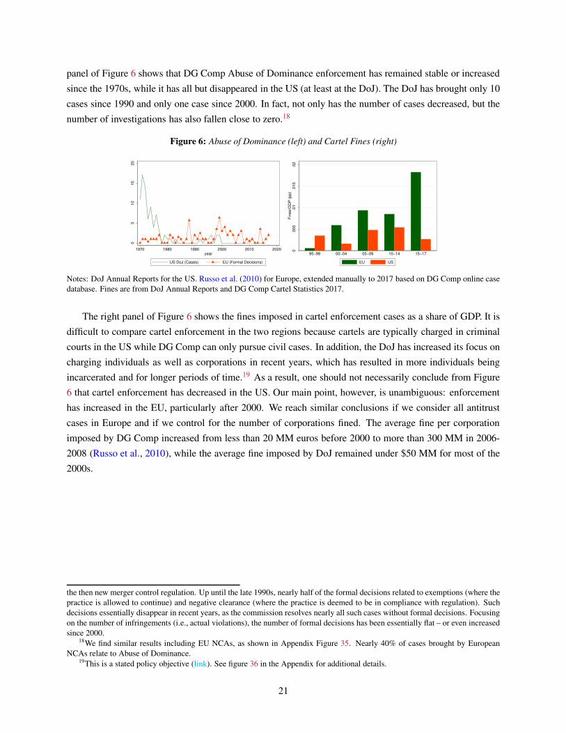
panel of Figure 6 shows that DG Comp Abuse of Dominance enforcement has remained stable or increased

since the 1970s, while it has all but disappeared in the US (at least at the DoJ). The DoJ has brought only 10

cases since 1990 and only one case since 2000. In fact, not only has the number of cases decreased, but the

number of investigations has also fallen close to zero.18

Figure 6: Abuse of Dominance (left) and Cartel Fines (right)

05

10

15

20

1970 1980 1990 2000 2010 2020year

US DoJ (Cases) EU (Formal Decisions)

0.0

05

.01

.015

.02

Fin

es/G

DP

(pp)

95−99 00−04 05−09 10−14 15−17

EU US

Notes: DoJ Annual Reports for the US. Russo et al. (2010) for Europe, extended manually to 2017 based on DG Comp online case

database. Fines are from DoJ Annual Reports and DG Comp Cartel Statistics 2017.

The right panel of Figure 6 shows the fines imposed in cartel enforcement cases as a share of GDP. It is

difficult to compare cartel enforcement in the two regions because cartels are typically charged in criminal

courts in the US while DG Comp can only pursue civil cases. In addition, the DoJ has increased its focus on

charging individuals as well as corporations in recent years, which has resulted in more individuals being

incarcerated and for longer periods of time.19 As a result, one should not necessarily conclude from Figure

6 that cartel enforcement has decreased in the US. Our main point, however, is unambiguous: enforcement

has increased in the EU, particularly after 2000. We reach similar conclusions if we consider all antitrust

cases in Europe and if we control for the number of corporations fined. The average fine per corporation

imposed by DG Comp increased from less than 20 MM euros before 2000 to more than 300 MM in 2006-

2008 (Russo et al., 2010), while the average fine imposed by DoJ remained under $50 MM for most of the

2000s.

the then new merger control regulation. Up until the late 1990s, nearly half of the formal decisions related to exemptions (where the

practice is allowed to continue) and negative clearance (where the practice is deemed to be in compliance with regulation). Such

decisions essentially disappear in recent years, as the commission resolves nearly all such cases without formal decisions. Focusing

on the number of infringements (i.e., actual violations), the number of formal decisions has been essentially flat – or even increased

since 2000.18We find similar results including EU NCAs, as shown in Appendix Figure 35. Nearly 40% of cases brought by European

NCAs relate to Abuse of Dominance.19This is a stated policy objective (link). See figure 36 in the Appendix for additional details.

21

2.3 Product Market Regulation

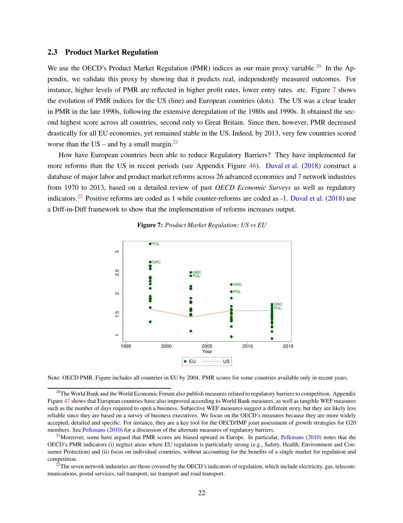
We use the OECD’s Product Market Regulation (PMR) indices as our main proxy variable.20 In the Ap-

pendix, we validate this proxy by showing that it predicts real, independently measured outcomes. For

instance, higher levels of PMR are reflected in higher profit rates, lower entry rates. etc. Figure 7 shows

the evolution of PMR indices for the US (line) and European countries (dots). The US was a clear leader

in PMR in the late 1990s, following the extensive deregulation of the 1980s and 1990s. It obtained the sec-

ond highest score across all countries, second only to Great Britain. Since then, however, PMR decreased

drastically for all EU economies, yet remained stable in the US. Indeed, by 2013, very few countries scored

worse than the US – and by a small margin.21

How have European countries been able to reduce Regulatory Barriers? They have implemented far

more reforms than the US in recent periods (see Appendix Figure 46). Duval et al. (2018) construct a

database of major labor and product market reforms across 26 advanced economies and 7 network industries

from 1970 to 2013, based on a detailed review of past OECD Economic Surveys as well as regulatory

indicators.22 Positive reforms are coded as 1 while counter-reforms are coded as -1. Duval et al. (2018) use

a Diff-in-Diff framework to show that the implementation of reforms increases output.

Figure 7: Product Market Regulation: US vs EU

GRC

GRC

GRC

GRC

POL

POL

POL

POL

11.5

22.5

3

1995 2000 2005 2010 2015Year

EU US

Note: OECD PMR. Figure includes all countries in EU by 2004. PMR scores for some countries available only in recent years.

20The World Bank and the World Economic Forum also publish measures related to regulatory barriers to competition. Appendix

Figure 47 shows that European countries have also improved according to World Bank measures, as well as tangible WEF measures

such as the number of days required to open a business. Subjective WEF measures suggest a different story, but they are likely less

reliable since they are based on a survey of business executives. We focus on the OECD’s measures because they are more widely

accepted, detailed and specific. For instance, they are a key tool for the OECD/IMF joint assessment of growth strategies for G20

members. See Pelkmans (2010) for a discussion of the alternate measures of regulatory barriers.21Moreover, some have argued that PMR scores are biased upward in Europe. In particular, Pelkmans (2010) notes that the

OECD’s PMR indicators (i) neglect areas where EU regulation is particularly strong (e.g., Safety, Health, Environment and Con-

sumer Protection) and (ii) focus on individual countries, without accounting for the benefits of a single market for regulation and

competition.22The seven network industries are those covered by the OECD’s indicators of regulation, which include electricity, gas, telecom-

munications, postal services, rail transport, air transport and road transport.

22

3 Test of Proposition 1(b): Deregulation Leads to Lower Markups

In this section we provide new evidence on the real effects of competition policies. We emphasize our new

contributions here, and we summarize other measures in the Appendix A where we review twenty proxies

for competition.23

Our empirical contribution is to tackle two limitations of the existing literature: the lack of prices and the

lack of plausible measures of changes in competition. We make progress on the first issue by using prices

from the International Comparison Program (ICP) and from STAN. We make progress on the second issue

by using measures of product market regulations at the country-year-industry level. We thus avoid using

concentration measures that are not always reliable, as extensively discussed in Syverson (2019), Shapiro

(2018) and Covarrubias et al. (2019).

3.1 Telecoms and Airlines

We start by focusing on two industries where regulatory changes are fairly well understood and where

we have multiple sources of prices data so we can be confident that our measures are correct. These two

industries also provide good examples of what PMRs can or cannot measure.

Telecoms

The Telecom industry used to be relatively competitive in the US. As Economides 2002 explained 20 years

ago:

“one of the key reasons for Europe’s lag in internet adoption is the fact [that] in most countries,

unlike the United States, consumers are charged per minute for local calls. The increasing use

of broadband connections is changing the model toward fixed monthly fees in Europe.”

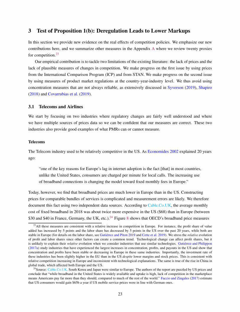
Today, however, we find that broadband prices are much lower in Europe than in the US. Constructing

prices for comparable bundles of services is complicated and measurement errors are likely. We therefore

document this fact using two independent data sources. According to Cable.Co.UK, the average monthly

cost of fixed broadband in 2018 was about twice more expensive in the US ($68) than in Europe (between

$30 and $40 in France, Germany, the UK, etc.).24 Figure 8 shows that OECD’s broadband price measures

23All these measures are consistent with a relative increase in competition in Europe. For instance, the profit share of value

added has increased by 5 points and the labor share has decreased by 5 points in the US over the past 20 years, while both are

stable in Europe (for details on the labor share, see Gutiérrez and Piton 2019 and Cette et al. 2019). We stress the relative evolution

of profit and labor shares since other factors can create a common trend. Technological change can affect profit shares, but it

is unlikely to explain their relative evolution when we consider industries that use similar technologies. Gutiérrez and Philippon

(2017a) study industries that have experienced the largest increases in concentration, profits, and payouts in the US and show that

concentration and profits have been stable or decreasing in Europe in these same industries. Importantly, the investment rate of

these industries has been slightly higher in the EU than in the US despite lower margins and stock prices. This is consistent with

relative competition increasing in Europe and inconsistent with technological explanations. The same is true of the rise in China in

global trade, which affected both Europe and the US.24Source: Cable.Co.UK. South Korea and Japan were similar to Europe. The authors of the report are puzzled by US prices and

conclude that “while broadband in the United States is widely available and uptake is high, lack of competition in the marketplace

means Americans pay far more than they should, compared to much of the rest of the world.” Faccio and Zingales (2017) estimate

that US consumers would gain $65b a year if US mobile service prices were in line with German ones.

23

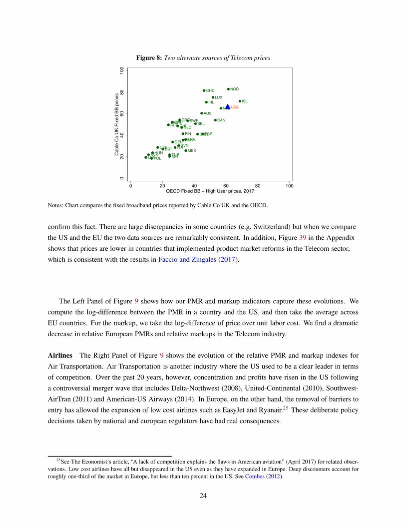
Figure 8: Two alternate sources of Telecom prices

AUS

AUT BELCAN

CHE

CHL

CZE

DEUDNK

ESP

EST

FIN

FRA

GBR

GRC

HUN

IRL ISL

ISR

ITA

JPN

LUX

LVA

MEX

NLD

NOR

NZL

POL

PRT

SVK

SVN

SWE

TUR

USA

020

40

60

80

100

Cable

Co U

K F

ixed B

B p

rices

0 20 40 60 80 100OECD Fixed BB − High User prices, 2017

Notes: Chart compares the fixed broadband prices reported by Cable Co UK and the OECD.

confirm this fact. There are large discrepancies in some countries (e.g. Switzerland) but when we compare

the US and the EU the two data sources are remarkably consistent. In addition, Figure 39 in the Appendix

shows that prices are lower in countries that implemented product market reforms in the Telecom sector,

which is consistent with the results in Faccio and Zingales (2017).

The Left Panel of Figure 9 shows how our PMR and markup indicators capture these evolutions. We

compute the log-difference between the PMR in a country and the US, and then take the average across

EU countries. For the markup, we take the log-difference of price over unit labor cost. We find a dramatic

decrease in relative European PMRs and relative markups in the Telecom industry.

Airlines The Right Panel of Figure 9 shows the evolution of the relative PMR and markup indexes for

Air Transportation. Air Transportation is another industry where the US used to be a clear leader in terms

of competition. Over the past 20 years, however, concentration and profits have risen in the US following

a controversial merger wave that includes Delta-Northwest (2008), United-Continental (2010), Southwest-

AirTran (2011) and American-US Airways (2014). In Europe, on the other hand, the removal of barriers to

entry has allowed the expansion of low cost airlines such as EasyJet and Ryanair.25 These deliberate policy

decisions taken by national and european regulators have had real consequences.

25See The Economist’s article, “A lack of competition explains the flaws in American aviation” (April 2017) for related obser-

vations. Low cost airlines have all but disappeared in the US even as they have expanded in Europe. Deep discounters account for

roughly one-third of the market in Europe, but less than ten percent in the US. See Combes (2012).

24

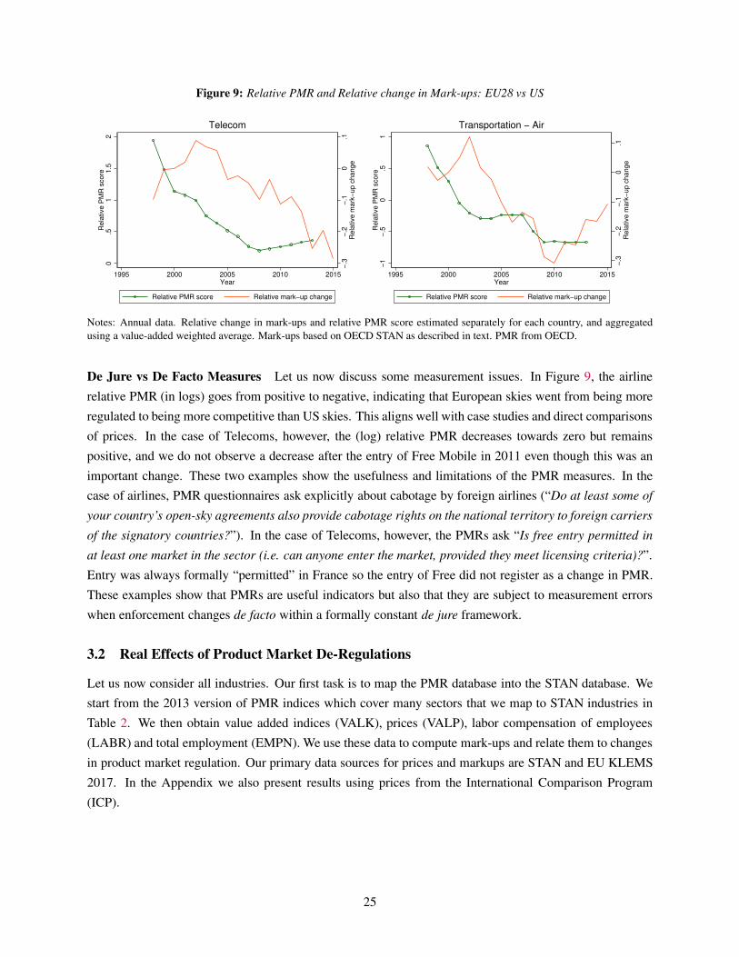
Figure 9: Relative PMR and Relative change in Mark-ups: EU28 vs US

−.3

−.2

−.1

0.1

Rela

tive m

ark

−up c

hange

0.5

11.5

2R

ela

tive P

MR

score

1995 2000 2005 2010 2015Year

Relative PMR score Relative mark−up change

Telecom

−.3

−.2

−.1

0.1

Rela

tive m

ark

−up c

hange

−1

−.5

0.5

1R

ela

tive P

MR

score

1995 2000 2005 2010 2015Year

Relative PMR score Relative mark−up change

Transportation − Air

Notes: Annual data. Relative change in mark-ups and relative PMR score estimated separately for each country, and aggregated

using a value-added weighted average. Mark-ups based on OECD STAN as described in text. PMR from OECD.

De Jure vs De Facto Measures Let us now discuss some measurement issues. In Figure 9, the airline

relative PMR (in logs) goes from positive to negative, indicating that European skies went from being more

regulated to being more competitive than US skies. This aligns well with case studies and direct comparisons

of prices. In the case of Telecoms, however, the (log) relative PMR decreases towards zero but remains

positive, and we do not observe a decrease after the entry of Free Mobile in 2011 even though this was an

important change. These two examples show the usefulness and limitations of the PMR measures. In the

case of airlines, PMR questionnaires ask explicitly about cabotage by foreign airlines (“Do at least some of

your country’s open-sky agreements also provide cabotage rights on the national territory to foreign carriers

of the signatory countries?”). In the case of Telecoms, however, the PMRs ask “Is free entry permitted in

at least one market in the sector (i.e. can anyone enter the market, provided they meet licensing criteria)?”.

Entry was always formally “permitted” in France so the entry of Free did not register as a change in PMR.

These examples show that PMRs are useful indicators but also that they are subject to measurement errors

when enforcement changes de facto within a formally constant de jure framework.

3.2 Real Effects of Product Market De-Regulations

Let us now consider all industries. Our first task is to map the PMR database into the STAN database. We

start from the 2013 version of PMR indices which cover many sectors that we map to STAN industries in

Table 2. We then obtain value added indices (VALK), prices (VALP), labor compensation of employees

(LABR) and total employment (EMPN). We use these data to compute mark-ups and relate them to changes

in product market regulation. Our primary data sources for prices and markups are STAN and EU KLEMS

2017. In the Appendix we also present results using prices from the International Comparison Program

(ICP).

25

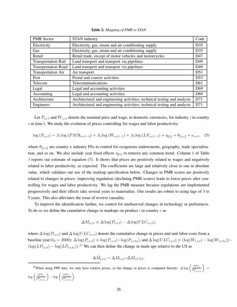
Table 2: Mapping of PMR to STAN

PMR Sector STAN industry Code

Electricity Electricity, gas, steam and air conditioning supply D35

Gas Electricity, gas, steam and air conditioning supply D35

Retail Retail trade, except of motor vehicles and motorcycles D47

Transportation Rail Land transport and transport via pipelines D49

Transportation Road Land transport and transport via pipelines D49

Transportation Air Air transport D51

Post Postal and courier activities D53

Telecom Telecommunications D61

Legal Legal and accounting activities D69

Accounting Legal and accounting activities D69

Architecture Architectural and engineering activities; technical testing and analysis D71

Engineers Architectural and engineering activities; technical testing and analysis D71

Let Pi,c,t and Wi,c,t denote the nominal price and wage, in domestic currencies, for industry i in country

c at time t. We study the evolution of prices controlling for wages and labor productivity:

log (Pi,c,t) = β1 log (PMRi,c,t−4) + β2 log (Wi,c,t−1) + β3 log (LPi,c,t−1) + η{t} + θ{i,c} + ǫi,c,t. (5)

where θ{i,c} are country x industry FEs to control for exogenous endowments, geography, trade specializa-

tion, and so on. We also include year fixed effects η{t} to remove any common trend. Column 1 of Table

3 reports our estimate of equation (5). It shows that prices are positively related to wages and negatively

related to labor productivity, as expected. The coefficients are large and relatively close to one in absolute

value, which validates our use of the markup specification below. Changes in PMR scores are positively

related to changes in prices: improving regulation (declining PMR scores) leads to lower prices after con-

trolling for wages and labor productivity. We lag the PMR measure because regulations are implemented

progressively and their effects take several years to materialize. Our results are robust to using lags of 3 to

5 years. This also alleviates the issue of reverse causality.

To improve the identification further, we control for unobserved changes in technology or preferences.

To do so we define the cumulative change in markups on product i in country c as

∆Mi,c,t ≡ ∆ log(Pi,c,t)−∆ log(ULCi,c,t),

where ∆ log(Pi,c,t) and ∆ log(ULCi,c,t) denote the cumulative change in prices and unit labor costs from a

baseline year (t0 = 2000): ∆ log(Pi,c,t) ≡ log(Pi,c,t)−log(Pi,c,t0), and ∆ log(ULCi,c,t) ≡ (log(Wi,c,t)− log(Wi,c,t0))−(log(LPi,c,t)− log(LPi,c,t0)).

26 We can then define the change in mark-ups relative to the US as

∆Mi,c,t = ∆Mi,c,t–∆Mi,US,t.

26When using PPP data, we only have relative prices, so the change in prices is computed directly: ∆ log

(

P euroi,c,t

P$i,US,t

)

=

log

(

P euroi,c,t

P$i,US,t

)

− log

(

P euroi,c,0

P$i,US,0

)

.

26

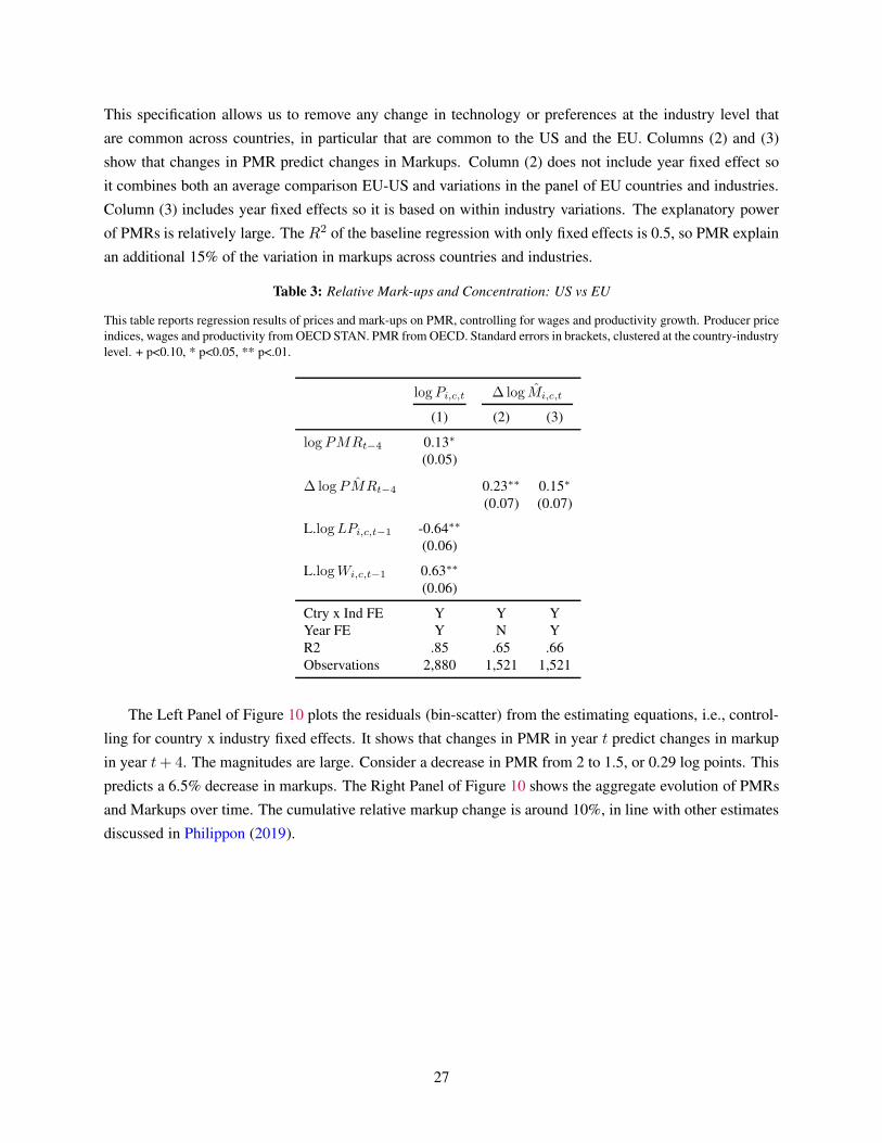
This specification allows us to remove any change in technology or preferences at the industry level that

are common across countries, in particular that are common to the US and the EU. Columns (2) and (3)

show that changes in PMR predict changes in Markups. Column (2) does not include year fixed effect so

it combines both an average comparison EU-US and variations in the panel of EU countries and industries.

Column (3) includes year fixed effects so it is based on within industry variations. The explanatory power

of PMRs is relatively large. The R2 of the baseline regression with only fixed effects is 0.5, so PMR explain

an additional 15% of the variation in markups across countries and industries.

Table 3: Relative Mark-ups and Concentration: US vs EU

This table reports regression results of prices and mark-ups on PMR, controlling for wages and productivity growth. Producer price

indices, wages and productivity from OECD STAN. PMR from OECD. Standard errors in brackets, clustered at the country-industry

level. + p<0.10, * p<0.05, ** p<.01.

logPi,c,t ∆ log Mi,c,t

(1) (2) (3)

logPMRt−4 0.13∗

(0.05)

∆ log ˆPMRt−4 0.23∗∗ 0.15∗

(0.07) (0.07)

L.logLPi,c,t−1 -0.64∗∗

(0.06)

L.logWi,c,t−1 0.63∗∗

(0.06)

Ctry x Ind FE Y Y Y

Year FE Y N Y

R2 .85 .65 .66

Observations 2,880 1,521 1,521

The Left Panel of Figure 10 plots the residuals (bin-scatter) from the estimating equations, i.e., control-

ling for country x industry fixed effects. It shows that changes in PMR in year t predict changes in markup

in year t+ 4. The magnitudes are large. Consider a decrease in PMR from 2 to 1.5, or 0.29 log points. This

predicts a 6.5% decrease in markups. The Right Panel of Figure 10 shows the aggregate evolution of PMRs

and Markups over time. The cumulative relative markup change is around 10%, in line with other estimates

discussed in Philippon (2019).

27

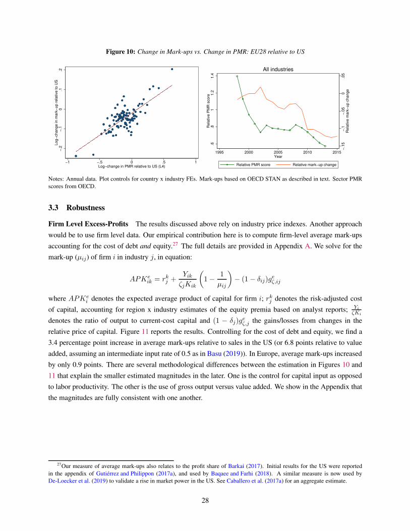
Figure 10: Change in Mark-ups vs. Change in PMR: EU28 relative to US

−.2

−.1

0.1

.2Log−

change in m

ark

−up r

ela

tive to U

S

−1 −.5 0 .5 1Log−change in PMR relative to US (L4)

−.1

5−

.1−

.05

0.0

5R

ela

tive m

ark

−up c

hange

.6.8

11.2

1.4

Rela

tive P

MR

score

1995 2000 2005 2010 2015Year

Relative PMR score Relative mark−up change

All industries

Notes: Annual data. Plot controls for country x industry FEs. Mark-ups based on OECD STAN as described in text. Sector PMR

scores from OECD.

3.3 Robustness

Firm Level Excess-Profits The results discussed above rely on industry price indexes. Another approach

would be to use firm level data. Our empirical contribution here is to compute firm-level average mark-ups

accounting for the cost of debt and equity.27 The full details are provided in Appendix A. We solve for the

mark-up (µij) of firm i in industry j, in equation:

APKeik = rkj +

Yik

ζjKik

(

1− 1

µij

)

− (1− δij)geζ,ij

where APKei denotes the expected average product of capital for firm i; rkj denotes the risk-adjusted cost

of capital, accounting for region x industry estimates of the equity premia based on analyst reports; Yi

ζKi

denotes the ratio of output to current-cost capital and (1 − δj)geζ,j the gains/losses from changes in the

relative price of capital. Figure 11 reports the results. Controlling for the cost of debt and equity, we find a

3.4 percentage point increase in average mark-ups relative to sales in the US (or 6.8 points relative to value

added, assuming an intermediate input rate of 0.5 as in Basu (2019)). In Europe, average mark-ups increased

by only 0.9 points. There are several methodological differences between the estimation in Figures 10 and

11 that explain the smaller estimated magnitudes in the later. One is the control for capital input as opposed

to labor productivity. The other is the use of gross output versus value added. We show in the Appendix that

the magnitudes are fully consistent with one another.

27Our measure of average mark-ups also relates to the profit share of Barkai (2017). Initial results for the US were reported

in the appendix of Gutiérrez and Philippon (2017a), and used by Baqaee and Farhi (2018). A similar measure is now used by

De-Loecker et al. (2019) to validate a rise in market power in the US. See Caballero et al. (2017a) for an aggregate estimate.

28

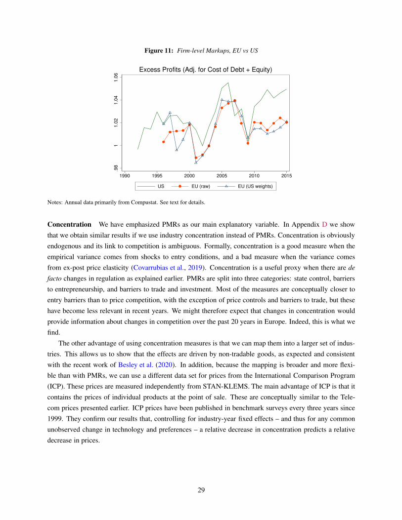
Figure 11: Firm-level Markups, EU vs US

.98

11.0

21.0

41.0

6

1990 1995 2000 2005 2010 2015

US EU (raw) EU (US weights)

Excess Profits (Adj. for Cost of Debt + Equity)

Notes: Annual data primarily from Compustat. See text for details.

Concentration We have emphasized PMRs as our main explanatory variable. In Appendix D we show

that we obtain similar results if we use industry concentration instead of PMRs. Concentration is obviously

endogenous and its link to competition is ambiguous. Formally, concentration is a good measure when the

empirical variance comes from shocks to entry conditions, and a bad measure when the variance comes

from ex-post price elasticity (Covarrubias et al., 2019). Concentration is a useful proxy when there are de

facto changes in regulation as explained earlier. PMRs are split into three categories: state control, barriers

to entrepreneurship, and barriers to trade and investment. Most of the measures are conceptually closer to

entry barriers than to price competition, with the exception of price controls and barriers to trade, but these

have become less relevant in recent years. We might therefore expect that changes in concentration would

provide information about changes in competition over the past 20 years in Europe. Indeed, this is what we

find.

The other advantage of using concentration measures is that we can map them into a larger set of indus-

tries. This allows us to show that the effects are driven by non-tradable goods, as expected and consistent

with the recent work of Besley et al. (2020). In addition, because the mapping is broader and more flexi-

ble than with PMRs, we can use a different data set for prices from the International Comparison Program

(ICP). These prices are measured independently from STAN-KLEMS. The main advantage of ICP is that it

contains the prices of individual products at the point of sale. These are conceptually similar to the Tele-

com prices presented earlier. ICP prices have been published in benchmark surveys every three years since

1999. They confirm our results that, controlling for industry-year fixed effects – and thus for any common

unobserved change in technology and preferences – a relative decrease in concentration predicts a relative

decrease in prices.

29

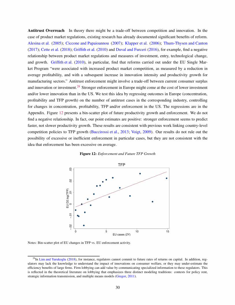
Antitrust Overreach In theory there might be a trade-off between competition and innovation. In the

case of product market regulations, existing research has already documented significant benefits of reform.

Alesina et al. (2005); Ciccone and Papaioannou (2007); Klapper et al. (2006); Thum-Thysen and Canton

(2017); Cette et al. (2018); Griffith et al. (2010) and Duval and Furceri (2016), for example, find a negative

relationship between product market regulations and measures of investment, entry, technological change,

and growth. Griffith et al. (2010), in particular, find that reforms carried out under the EU Single Mar-

ket Program “were associated with increased product market competition, as measured by a reduction in

average profitability, and with a subsequent increase in innovation intensity and productivity growth for

manufacturing sectors.” Antitrust enforcement might involve a trade-off between current consumer surplus

and innovation or investment.28 Stronger enforcement in Europe might come at the cost of lower investment

and/or lower innovation than in the US. We test this idea by regressing outcomes in Europe (concentration,

profitability and TFP growth) on the number of antitrust cases in the corresponding industry, controlling

for changes in concentration, profitability, TFP and/or enforcement in the US. The regressions are in the

Appendix. Figure 12 presents a bin-scatter plot of future productivity growth and enforcement. We do not

find a negative relationship. In fact, our point estimates are positive: stronger enforcement seems to predict

faster, not slower productivity growth. These results are consistent with previous work linking country-level

competition policies to TFP growth (Buccirossi et al., 2013; Voigt, 2009). Our results do not rule out the

possibility of excessive or inefficient enforcement in particular cases, but they are not consistent with the

idea that enforcement has been excessive on average.

Figure 12: Enforcement and Future TFP Growth

−.0

2−

.01

0.0

1.0

2.0

3E

U D

2.log(T

FP

)

0 5 10 15EU cases (2Y)

TFP

Notes: Bin-scatter plot of EU changes in TFP vs. EU enforcement activity.

28In Lim and Yurukoglu (2018), for instance, regulators cannot commit to future rates of returns on capital. In addition, reg-

ulators may lack the knowledge to understand the impact of innovations on consumer welfare, or they may under-estimate the

efficiency benefits of large firms. Firm lobbying can add value by communicating specialized information to these regulators. This

is reflected in the theoretical literature on lobbying that emphasizes three distinct modeling traditions: contests for policy rent,

strategic information transmission, and multiple means models (Gregor, 2011).

30

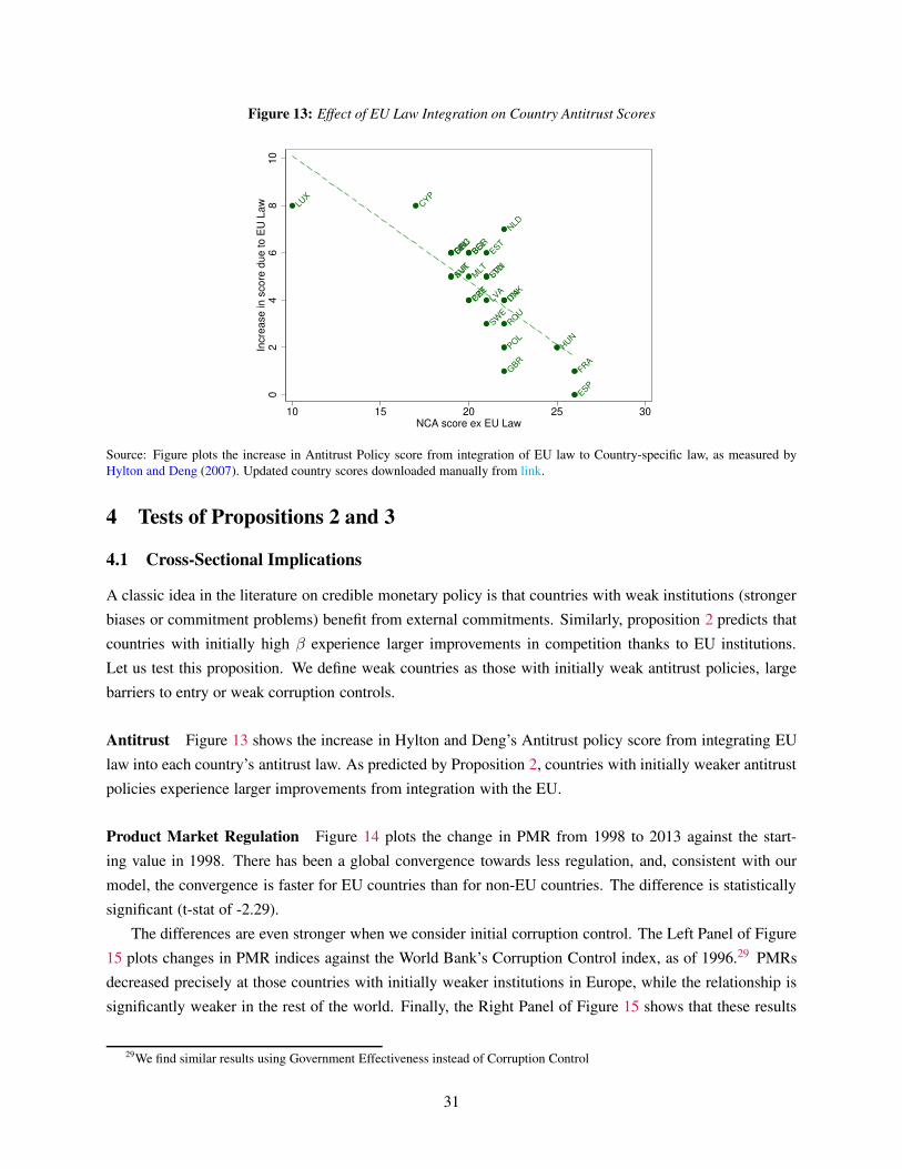
Figure 13: Effect of EU Law Integration on Country Antitrust Scores

AUT

BELBG

R

CYP

CZE

DEU

DNK

ESP

ESTFIN

FRA

GBR

GRC

HUN

ITA

LTU

LUX

LVA

MLT

NLD

POL

PRT

ROU

SVKSVN

SWE

02

46

810

Incre

ase in s

core

due to E

U L

aw

10 15 20 25 30NCA score ex EU Law

Source: Figure plots the increase in Antitrust Policy score from integration of EU law to Country-specific law, as measured by

Hylton and Deng (2007). Updated country scores downloaded manually from link.

4 Tests of Propositions 2 and 3

4.1 Cross-Sectional Implications

A classic idea in the literature on credible monetary policy is that countries with weak institutions (stronger

biases or commitment problems) benefit from external commitments. Similarly, proposition 2 predicts that

countries with initially high β experience larger improvements in competition thanks to EU institutions.

Let us test this proposition. We define weak countries as those with initially weak antitrust policies, large

barriers to entry or weak corruption controls.

Antitrust Figure 13 shows the increase in Hylton and Deng’s Antitrust policy score from integrating EU

law into each country’s antitrust law. As predicted by Proposition 2, countries with initially weaker antitrust

policies experience larger improvements from integration with the EU.

Product Market Regulation Figure 14 plots the change in PMR from 1998 to 2013 against the start-

ing value in 1998. There has been a global convergence towards less regulation, and, consistent with our

model, the convergence is faster for EU countries than for non-EU countries. The difference is statistically

significant (t-stat of -2.29).

The differences are even stronger when we consider initial corruption control. The Left Panel of Figure

15 plots changes in PMR indices against the World Bank’s Corruption Control index, as of 1996.29 PMRs

decreased precisely at those countries with initially weaker institutions in Europe, while the relationship is

significantly weaker in the rest of the world. Finally, the Right Panel of Figure 15 shows that these results

29We find similar results using Government Effectiveness instead of Corruption Control

31

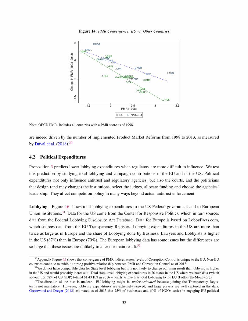
Figure 14: PMR Convergence: EU vs. Other Countries

AUT BEL

CZE

DEU

DNK

ESP

FIN

FRA

GBR

GRC

HUN

IRL

ITA

NLD

POL

PRT

SWEAUS

CAN

CHE

ISL

JPN KOR

MEX

NOR

NZL

TUR

USA

−1.5

−1

−.5

0C

hange in P

MR

(1998−

2013)

1.5 2 2.5 3 3.5PMR (1998)

EU Non−EU

Note: OECD PMR. Includes all countries with a PMR score as of 1998.

are indeed driven by the number of implemented Product Market Reforms from 1998 to 2013, as measured

by Duval et al. (2018).30

4.2 Political Expenditures

Proposition 3 predicts lower lobbying expenditures when regulators are more difficult to influence. We test

this prediction by studying total lobbying and campaign contributions in the EU and in the US. Political

expenditures not only influence antitrust and regulatory agencies, but also the courts, and the politicians

that design (and may change) the institutions, select the judges, allocate funding and choose the agencies’

leadership. They affect competition policy in many ways beyond actual antitrust enforcement.

Lobbying Figure 16 shows total lobbying expenditures to the US Federal government and to European

Union institutions.31 Data for the US come from the Center for Responsive Politics, which in turn sources

data from the Federal Lobbying Disclosure Act Database. Data for Europe is based on LobbyFacts.com,

which sources data from the EU Transparency Register. Lobbying expenditures in the US are more than

twice as large as in Europe and the share of Lobbying done by Business, Lawyers and Lobbyists is higher

in the US (87%) than in Europe (70%). The European lobbying data has some issues but the differences are

so large that these issues are unlikely to alter our main result.32

30Appendix Figure 45 shows that convergence of PMR indices across levels of Corruption Control is unique to the EU. Non-EU

countries continue to exhibit a strong positive relationship between PMR and Corruption Control as of 2013.31We do not have comparable data for State level lobbying but it is not likely to change our main result that lobbying is higher

in the US and would probably increase it. Total state-level lobbying expenditures in 20 states in the US where we have data (which

account for 58% of US GDP) totaled $1.43 BN in 2016 – nearly as much as total Lobbying to the EU (FollowTheMoney.org).32The direction of the bias is unclear. EU lobbying might be under-estimated because joining the Transparency Regis-

ter is not mandatory. However, lobbying expenditures are extremely skewed, and large players are well captured in the data.

Greenwood and Dreger (2013) estimated as of 2013 that 75% of businesses and 60% of NGOs active in engaging EU political

32

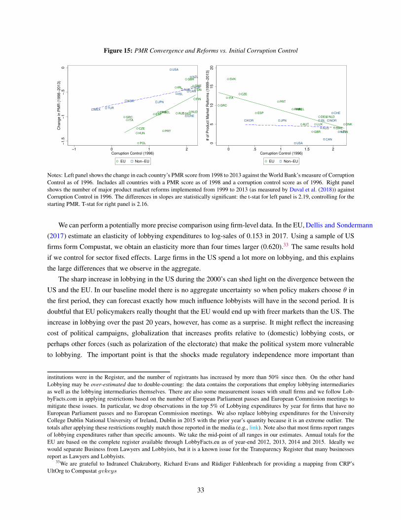
Figure 15: PMR Convergence and Reforms vs. Initial Corruption Control

AUTBEL

CZE

DEU

DNK

ESP

FIN

FRA

GBR

GRC

HUN

IRL

ITA

NLD

POL

PRT

SWE

AUSCAN

CHE

ISL

JPNKOR

MEX

NOR

NZL

TUR

USA

−1.5

−1

−.5

0C

hange in P

MR

(1998−

2013)

−1 0 1 2Corruption Control (1996)

EU Non−EU

AUT

BEL

CZE

DEU

DNK

ESP

FIN

FRA

GBR

GRC

IRL

ITA

LUX

NLD

PRT

SVK

SWEAUS

CAN

CHE

ISLJPNKOR NOR

NZL

USA05

10

15

20

# o

f P

roduct M

ark

et R

efo

rms (

1999−

2013)

0 .5 1 1.5 2Corruption Control (1996)

EU Non−EU

Notes: Left panel shows the change in each country’s PMR score from 1998 to 2013 against the World Bank’s measure of Corruption

Control as of 1996. Includes all countries with a PMR score as of 1998 and a corruption control score as of 1996. Right panel

shows the number of major product market reforms implemented from 1999 to 2013 (as measured by Duval et al. (2018)) against

Corruption Control in 1996. The differences in slopes are statistically significant: the t-stat for left panel is 2.19, controlling for the

starting PMR. T-stat for right panel is 2.16.

We can perform a potentially more precise comparison using firm-level data. In the EU, Dellis and Sondermann

(2017) estimate an elasticity of lobbying expenditures to log-sales of 0.153 in 2017. Using a sample of US

firms form Compustat, we obtain an elasticity more than four times larger (0.620).33 The same results hold

if we control for sector fixed effects. Large firms in the US spend a lot more on lobbying, and this explains

the large differences that we observe in the aggregate.

The sharp increase in lobbying in the US during the 2000’s can shed light on the divergence between the

US and the EU. In our baseline model there is no aggregate uncertainty so when policy makers choose θ in

the first period, they can forecast exactly how much influence lobbyists will have in the second period. It is

doubtful that EU policymakers really thought that the EU would end up with freer markets than the US. The

increase in lobbying over the past 20 years, however, has come as a surprise. It might reflect the increasing

cost of political campaigns, globalization that increases profits relative to (domestic) lobbying costs, or

perhaps other forces (such as polarization of the electorate) that make the political system more vulnerable

to lobbying. The important point is that the shocks made regulatory independence more important than

institutions were in the Register, and the number of registrants has increased by more than 50% since then. On the other hand

Lobbying may be over-estimated due to double-counting: the data contains the corporations that employ lobbying intermediaries

as well as the lobbying intermediaries themselves. There are also some measurement issues with small firms and we follow Lob-

byFacts.com in applying restrictions based on the number of European Parliament passes and European Commission meetings to

mitigate these issues. In particular, we drop observations in the top 5% of Lobbying expenditures by year for firms that have no

European Parliament passes and no European Commission meetings. We also replace lobbying expenditures for the University

College Dublin National University of Ireland, Dublin in 2015 with the prior year’s quantity because it is an extreme outlier. The

totals after applying these restrictions roughly match those reported in the media (e.g., link). Note also that most firms report ranges

of lobbying expenditures rather than specific amounts. We take the mid-point of all ranges in our estimates. Annual totals for the

EU are based on the complete register available through LobbyFacts.eu as of year-end 2012, 2013, 2014 and 2015. Ideally we

would separate Business from Lawyers and Lobbyists, but it is a known issue for the Transparency Register that many businesses

report as Lawyers and Lobbyists.33We are grateful to Indraneel Chakraborty, Richard Evans and Rüdiger Fahlenbrach for providing a mapping from CRP’s

UltOrg to Compustat gvkeys

33

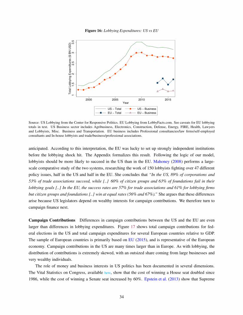
Figure 16: Lobbying Expenditures: US vs EU

11.5

22.5

33.5

Tota

l Lobbyin

g E

xpenditure

s (

$ B

N U

SD

)

2000 2005 2010 2015Year

US − Total US − Business

EU − Total EU − Business

Source: US Lobbying from the Center for Responsive Politics. EU Lobbying from LobbyFacts.com. See caveats for EU lobbying

totals in text. US Business sector includes Agribusiness, Electronics, Construction, Defense, Energy, FIRE, Health, Lawyers

and Lobbyists, Misc. Business and Transportation. EU business includes Professional consultancies/law firms/self-employed

consultants and In-house lobbyists and trade/business/professional associations.

anticipated. According to this interpretation, the EU was lucky to set up strongly independent institutions

before the lobbying shock hit. The Appendix formalizes this result. Following the logic of our model,

lobbyists should be more likely to succeed in the US than in the EU. Mahoney (2008) performs a large-

scale comparative study of the two systems, researching the work of 150 lobbyists fighting over 47 different

policy issues, half in the US and half in the EU. She concludes that “In the US, 89% of corporations and

53% of trade associations succeed, while [..] 60% of citizen groups and 63% of foundations fail in their

lobbying goals [..] In the EU, the success rates are 57% for trade associations and 61% for lobbying firms

but citizen groups and foundations [..] win at equal rates (56% and 67%).” She argues that these differences

arise because US legislators depend on wealthy interests for campaign contributions. We therefore turn to

campaign finance next.

Campaign Contributions Differences in campaign contributions between the US and the EU are even

larger than differences in lobbying expenditures. Figure 17 shows total campaign contributions for fed-

eral elections in the US and total campaign expenditures for several European countries relative to GDP.

The sample of European countries is primarily based on EU (2015), and is representative of the European

economy. Campaign contributions in the US are many times larger than in Europe. As with lobbying, the

distribution of contributions is extremely skewed, with an outsized share coming from large businesses and

very wealthy individuals.

The role of money and business interests in US politics has been documented in several dimensions.

The Vital Statistics on Congress, available here, show that the cost of winning a House seat doubled since

1986, while the cost of winning a Senate seat increased by 60%. Epstein et al. (2013) show that Supreme

34

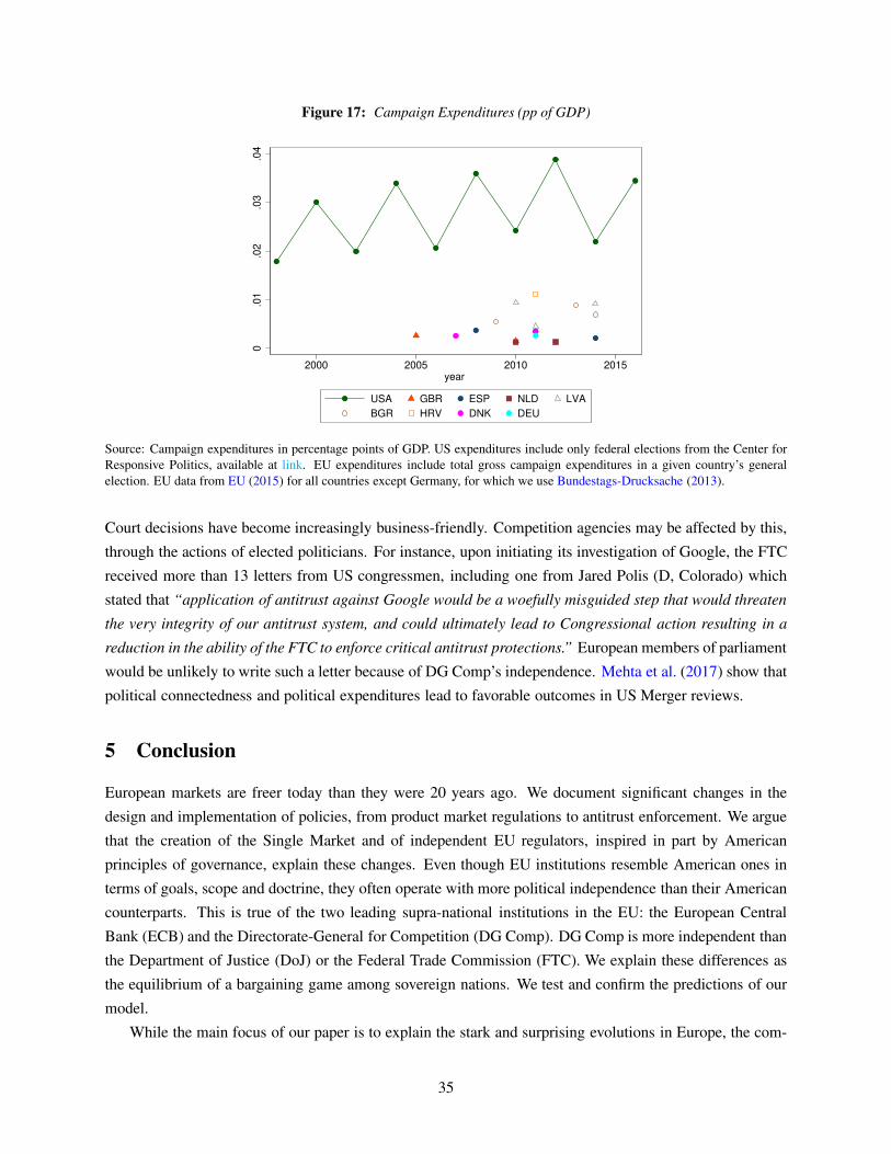
Figure 17: Campaign Expenditures (pp of GDP)

0.0

1.0

2.0

3.0

4

2000 2005 2010 2015year

USA GBR ESP NLD LVA

BGR HRV DNK DEU

Source: Campaign expenditures in percentage points of GDP. US expenditures include only federal elections from the Center for

Responsive Politics, available at link. EU expenditures include total gross campaign expenditures in a given country’s general

election. EU data from EU (2015) for all countries except Germany, for which we use Bundestags-Drucksache (2013).

Court decisions have become increasingly business-friendly. Competition agencies may be affected by this,

through the actions of elected politicians. For instance, upon initiating its investigation of Google, the FTC

received more than 13 letters from US congressmen, including one from Jared Polis (D, Colorado) which

stated that “application of antitrust against Google would be a woefully misguided step that would threaten

the very integrity of our antitrust system, and could ultimately lead to Congressional action resulting in a

reduction in the ability of the FTC to enforce critical antitrust protections.” European members of parliament

would be unlikely to write such a letter because of DG Comp’s independence. Mehta et al. (2017) show that

political connectedness and political expenditures lead to favorable outcomes in US Merger reviews.

5 Conclusion

European markets are freer today than they were 20 years ago. We document significant changes in the

design and implementation of policies, from product market regulations to antitrust enforcement. We argue

that the creation of the Single Market and of independent EU regulators, inspired in part by American

principles of governance, explain these changes. Even though EU institutions resemble American ones in

terms of goals, scope and doctrine, they often operate with more political independence than their American

counterparts. This is true of the two leading supra-national institutions in the EU: the European Central

Bank (ECB) and the Directorate-General for Competition (DG Comp). DG Comp is more independent than

the Department of Justice (DoJ) or the Federal Trade Commission (FTC). We explain these differences as

the equilibrium of a bargaining game among sovereign nations. We test and confirm the predictions of our

model.

While the main focus of our paper is to explain the stark and surprising evolutions in Europe, the com-

35

parison with Europe is useful to understand the US experience, and especially the rise in lobbying which is

an important topic for future research. We have studied the relative evolution of European markets, arguing

that they are more competitive than they used to be, and also that the gap with the US has closed.This opens

several obvious questions for future research. Is the catch-up complete? Has there been a reversal? If so,

in which industries? And most importantly, are American markets less competitive than they were in an

absolute sense?

36

References

Acemoglu, D., S. Johnson, and J. A. Robinson (2005, 12). Chapter 6 institutions as a fundamental cause of

long-run growth. 1, 385–472.

Alemani, E., C. Klein, I. Koske, C. Vitale, and I. Wanner (2013). New indicators of competition law and

policy in 2013 for oecd and non-oecd countries.

Alesina, A., S. Ardagna, G. Nicoletti, and F. Schiantarelli (2005, jun). Regulation and investment. Journal

of the European Economic Association 3(4), 791–825.

Alesina, A. and F. Giavazzi (2006). The Future of Europe: Reform or Decline. MIT Press. Translations:

Greek, Korean, Italian, Portuguese, Spanish.

Autor, D., D. Dorn, L. Katz, C. Patterson, and J. V. Reenen (2017). Concentrating on the fall of the labor

share. AER Papers and Proceedings 107(5), 180–185.

Bailey, J. and D. Thomas (2015). Regulating away competition: The effect of regulation on entrepreneurship

and employment. Mercatus Working Paper.

Bajgar, M., G. Berlingieri, S. Calligaris, C. Criscuolo, and J. Timmis (2019). Industry concentration in

europe and north america. Technical report, OECD.

Baqaee, D. R. and E. Farhi (2018). The macroeconomic impact of microeconomic shocks: Beyond hulten’s

theorem.

Barkai, S. (2017). Declining labor and capital shares. University of Chicago.

Barro, R. J. and D. B. Gordon (1983). Rules, discretion and reputation in a model of monetary policy.

Journal of Monetary Economics 12(1), 101 – 121.

Basu, S. (2019). Are price-cost mark-ups rising in the united states? a discussion of the evidence.

Berger, D. (1998). Law and Competition in Twentieth Century Europe.

Bergman, M., M. Coate, M. Jakobsson, and S. Ulrik (2010). Comparing merger policies in the european

union and the united states. Review of Industrial Organization 36, 305–331.

Bergman, M. A., M. B. Coate, A. T.V.Mai, and S. W. Ulrick (2016). Does merger policy converge after the

2004 european union reforms? Working Paper.

Besley, T., N. Fontana, and N. Limodio (2020). Anti-trust policies and profitability in non-traded sectors.

Working paper.

Bork, R. (1978). The Antitrust Paradox. New York: Basic Books.

Bradford, A. and A. S. Chilton (2018, sep). Competition law around the world from 1889 to 2010: The

competition law index. Journal of Competition Law & Economics 14(3), 393–432.

37

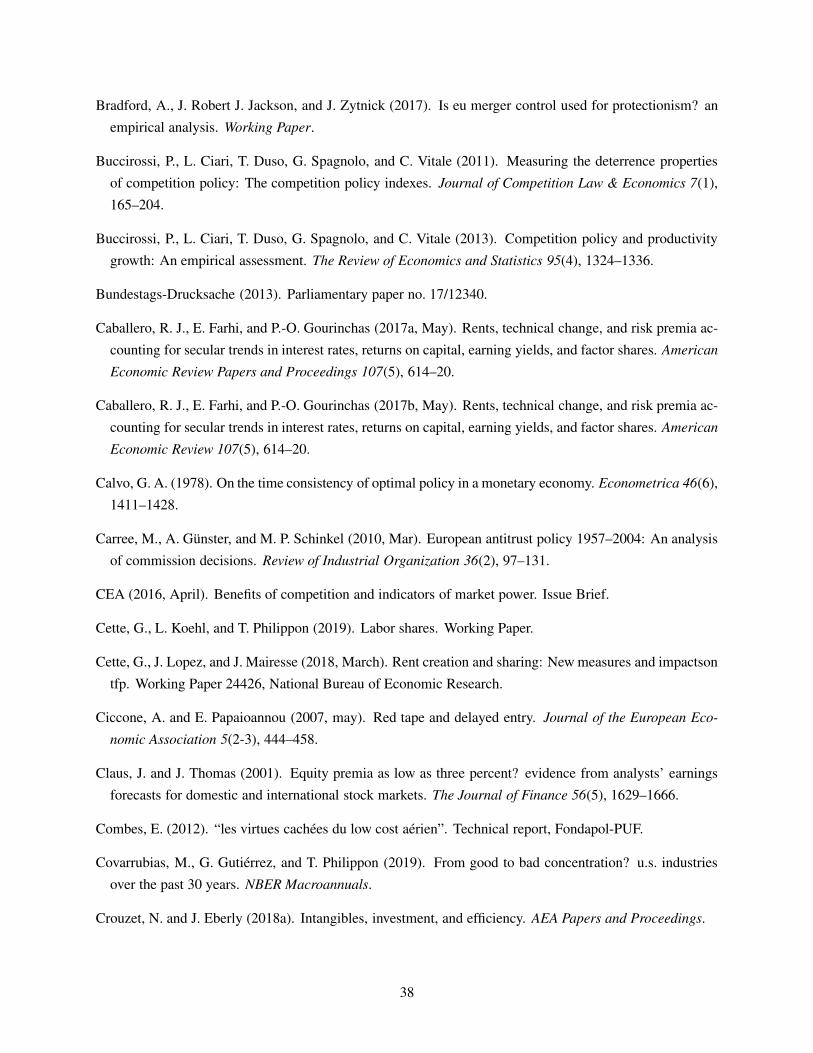
Bradford, A., J. Robert J. Jackson, and J. Zytnick (2017). Is eu merger control used for protectionism? an

empirical analysis. Working Paper.

Buccirossi, P., L. Ciari, T. Duso, G. Spagnolo, and C. Vitale (2011). Measuring the deterrence properties

of competition policy: The competition policy indexes. Journal of Competition Law & Economics 7(1),

165–204.

Buccirossi, P., L. Ciari, T. Duso, G. Spagnolo, and C. Vitale (2013). Competition policy and productivity

growth: An empirical assessment. The Review of Economics and Statistics 95(4), 1324–1336.

Bundestags-Drucksache (2013). Parliamentary paper no. 17/12340.

Caballero, R. J., E. Farhi, and P.-O. Gourinchas (2017a, May). Rents, technical change, and risk premia ac-

counting for secular trends in interest rates, returns on capital, earning yields, and factor shares. American

Economic Review Papers and Proceedings 107(5), 614–20.

Caballero, R. J., E. Farhi, and P.-O. Gourinchas (2017b, May). Rents, technical change, and risk premia ac-

counting for secular trends in interest rates, returns on capital, earning yields, and factor shares. American

Economic Review 107(5), 614–20.

Calvo, G. A. (1978). On the time consistency of optimal policy in a monetary economy. Econometrica 46(6),

1411–1428.

Carree, M., A. Günster, and M. P. Schinkel (2010, Mar). European antitrust policy 1957–2004: An analysis

of commission decisions. Review of Industrial Organization 36(2), 97–131.

CEA (2016, April). Benefits of competition and indicators of market power. Issue Brief.

Cette, G., L. Koehl, and T. Philippon (2019). Labor shares. Working Paper.

Cette, G., J. Lopez, and J. Mairesse (2018, March). Rent creation and sharing: New measures and impactson

tfp. Working Paper 24426, National Bureau of Economic Research.

Ciccone, A. and E. Papaioannou (2007, may). Red tape and delayed entry. Journal of the European Eco-

nomic Association 5(2-3), 444–458.

Claus, J. and J. Thomas (2001). Equity premia as low as three percent? evidence from analysts’ earnings

forecasts for domestic and international stock markets. The Journal of Finance 56(5), 1629–1666.

Combes, E. (2012). “les virtues cachées du low cost aérien”. Technical report, Fondapol-PUF.

Covarrubias, M., G. Gutiérrez, and T. Philippon (2019). From good to bad concentration? u.s. industries

over the past 30 years. NBER Macroannuals.

Crouzet, N. and J. Eberly (2018a). Intangibles, investment, and efficiency. AEA Papers and Proceedings.

38

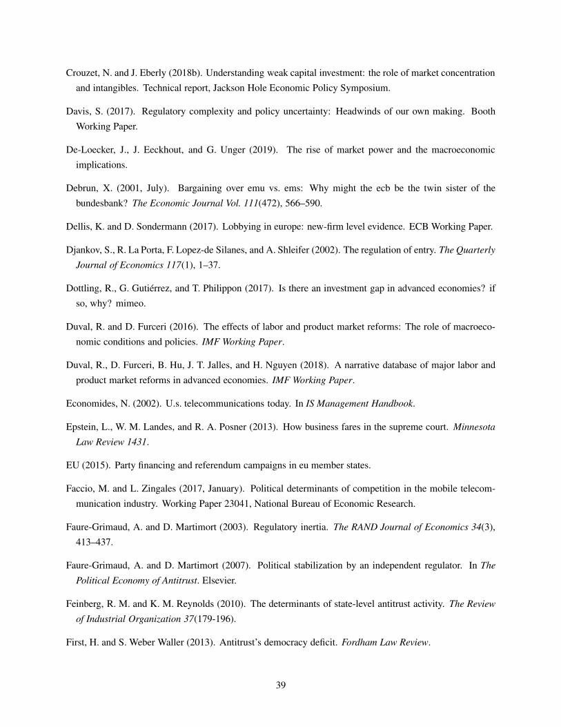
Crouzet, N. and J. Eberly (2018b). Understanding weak capital investment: the role of market concentration

and intangibles. Technical report, Jackson Hole Economic Policy Symposium.

Davis, S. (2017). Regulatory complexity and policy uncertainty: Headwinds of our own making. Booth

Working Paper.

De-Loecker, J., J. Eeckhout, and G. Unger (2019). The rise of market power and the macroeconomic

implications.

Debrun, X. (2001, July). Bargaining over emu vs. ems: Why might the ecb be the twin sister of the

bundesbank? The Economic Journal Vol. 111(472), 566–590.

Dellis, K. and D. Sondermann (2017). Lobbying in europe: new-firm level evidence. ECB Working Paper.

Djankov, S., R. La Porta, F. Lopez-de Silanes, and A. Shleifer (2002). The regulation of entry. The Quarterly

Journal of Economics 117(1), 1–37.

Dottling, R., G. Gutiérrez, and T. Philippon (2017). Is there an investment gap in advanced economies? if

so, why? mimeo.

Duval, R. and D. Furceri (2016). The effects of labor and product market reforms: The role of macroeco-

nomic conditions and policies. IMF Working Paper.

Duval, R., D. Furceri, B. Hu, J. T. Jalles, and H. Nguyen (2018). A narrative database of major labor and

product market reforms in advanced economies. IMF Working Paper.

Economides, N. (2002). U.s. telecommunications today. In IS Management Handbook.

Epstein, L., W. M. Landes, and R. A. Posner (2013). How business fares in the supreme court. Minnesota

Law Review 1431.

EU (2015). Party financing and referendum campaigns in eu member states.

Faccio, M. and L. Zingales (2017, January). Political determinants of competition in the mobile telecom-

munication industry. Working Paper 23041, National Bureau of Economic Research.

Faure-Grimaud, A. and D. Martimort (2003). Regulatory inertia. The RAND Journal of Economics 34(3),

413–437.

Faure-Grimaud, A. and D. Martimort (2007). Political stabilization by an independent regulator. In The

Political Economy of Antitrust. Elsevier.

Feinberg, R. M. and K. M. Reynolds (2010). The determinants of state-level antitrust activity. The Review

of Industrial Organization 37(179-196).

First, H. and S. Weber Waller (2013). Antitrust’s democracy deficit. Fordham Law Review.

39

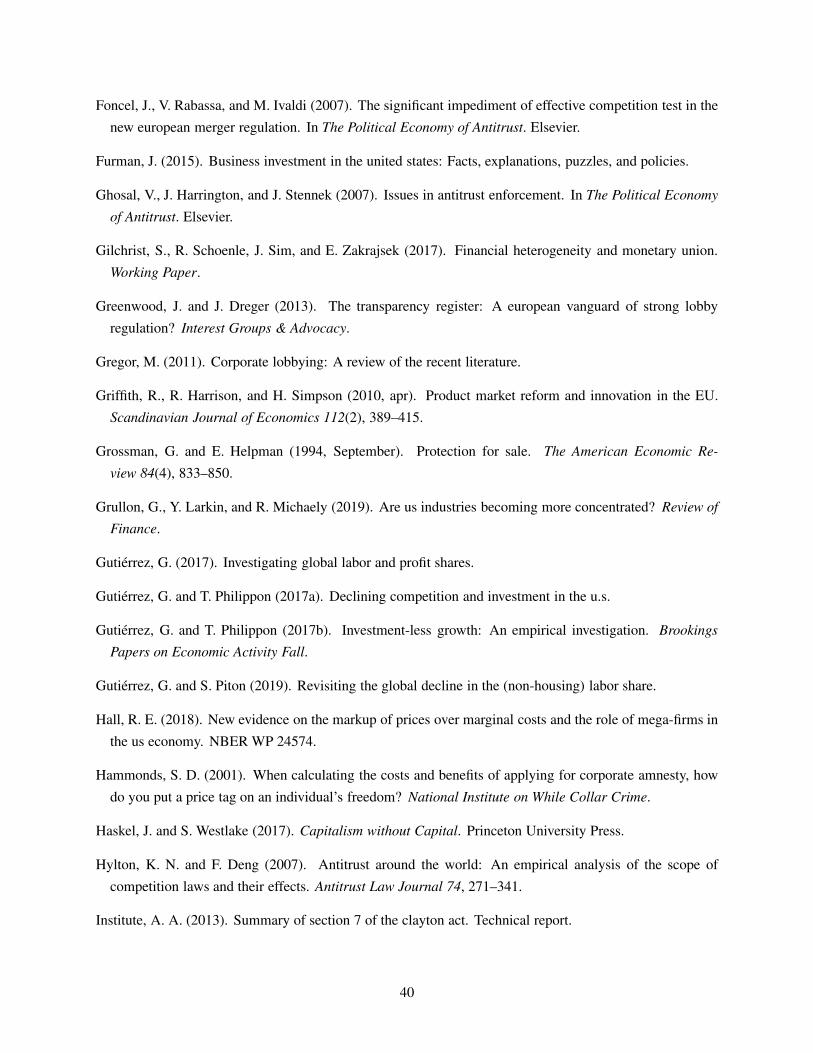
Foncel, J., V. Rabassa, and M. Ivaldi (2007). The significant impediment of effective competition test in the

new european merger regulation. In The Political Economy of Antitrust. Elsevier.

Furman, J. (2015). Business investment in the united states: Facts, explanations, puzzles, and policies.

Ghosal, V., J. Harrington, and J. Stennek (2007). Issues in antitrust enforcement. In The Political Economy

of Antitrust. Elsevier.

Gilchrist, S., R. Schoenle, J. Sim, and E. Zakrajsek (2017). Financial heterogeneity and monetary union.

Working Paper.

Greenwood, J. and J. Dreger (2013). The transparency register: A european vanguard of strong lobby

regulation? Interest Groups & Advocacy.

Gregor, M. (2011). Corporate lobbying: A review of the recent literature.

Griffith, R., R. Harrison, and H. Simpson (2010, apr). Product market reform and innovation in the EU.

Scandinavian Journal of Economics 112(2), 389–415.

Grossman, G. and E. Helpman (1994, September). Protection for sale. The American Economic Re-

view 84(4), 833–850.

Grullon, G., Y. Larkin, and R. Michaely (2019). Are us industries becoming more concentrated? Review of

Finance.

Gutiérrez, G. (2017). Investigating global labor and profit shares.

Gutiérrez, G. and T. Philippon (2017a). Declining competition and investment in the u.s.

Gutiérrez, G. and T. Philippon (2017b). Investment-less growth: An empirical investigation. Brookings

Papers on Economic Activity Fall.

Gutiérrez, G. and S. Piton (2019). Revisiting the global decline in the (non-housing) labor share.

Hall, R. E. (2018). New evidence on the markup of prices over marginal costs and the role of mega-firms in

the us economy. NBER WP 24574.

Hammonds, S. D. (2001). When calculating the costs and benefits of applying for corporate amnesty, how

do you put a price tag on an individual’s freedom? National Institute on While Collar Crime.

Haskel, J. and S. Westlake (2017). Capitalism without Capital. Princeton University Press.

Hylton, K. N. and F. Deng (2007). Antitrust around the world: An empirical analysis of the scope of

competition laws and their effects. Antitrust Law Journal 74, 271–341.

Institute, A. A. (2013). Summary of section 7 of the clayton act. Technical report.

40

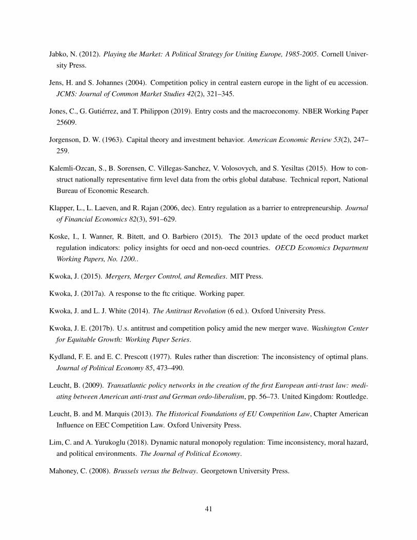
Jabko, N. (2012). Playing the Market: A Political Strategy for Uniting Europe, 1985-2005. Cornell Univer-

sity Press.

Jens, H. and S. Johannes (2004). Competition policy in central eastern europe in the light of eu accession.

JCMS: Journal of Common Market Studies 42(2), 321–345.

Jones, C., G. Gutiérrez, and T. Philippon (2019). Entry costs and the macroeconomy. NBER Working Paper

25609.

Jorgenson, D. W. (1963). Capital theory and investment behavior. American Economic Review 53(2), 247–

259.

Kalemli-Ozcan, S., B. Sorensen, C. Villegas-Sanchez, V. Volosovych, and S. Yesiltas (2015). How to con-

struct nationally representative firm level data from the orbis global database. Technical report, National

Bureau of Economic Research.

Klapper, L., L. Laeven, and R. Rajan (2006, dec). Entry regulation as a barrier to entrepreneurship. Journal

of Financial Economics 82(3), 591–629.

Koske, I., I. Wanner, R. Bitett, and O. Barbiero (2015). The 2013 update of the oecd product market

regulation indicators: policy insights for oecd and non-oecd countries. OECD Economics Department

Working Papers, No. 1200..

Kwoka, J. (2015). Mergers, Merger Control, and Remedies. MIT Press.

Kwoka, J. (2017a). A response to the ftc critique. Working paper.

Kwoka, J. and L. J. White (2014). The Antitrust Revolution (6 ed.). Oxford University Press.

Kwoka, J. E. (2017b). U.s. antitrust and competition policy amid the new merger wave. Washington Center

for Equitable Growth: Working Paper Series.

Kydland, F. E. and E. C. Prescott (1977). Rules rather than discretion: The inconsistency of optimal plans.

Journal of Political Economy 85, 473–490.

Leucht, B. (2009). Transatlantic policy networks in the creation of the first European anti-trust law: medi-

ating between American anti-trust and German ordo-liberalism, pp. 56–73. United Kingdom: Routledge.

Leucht, B. and M. Marquis (2013). The Historical Foundations of EU Competition Law, Chapter American

Influence on EEC Competition Law. Oxford University Press.

Lim, C. and A. Yurukoglu (2018). Dynamic natural monopoly regulation: Time inconsistency, moral hazard,

and political environments. The Journal of Political Economy.

Mahoney, C. (2008). Brussels versus the Beltway. Georgetown University Press.

41

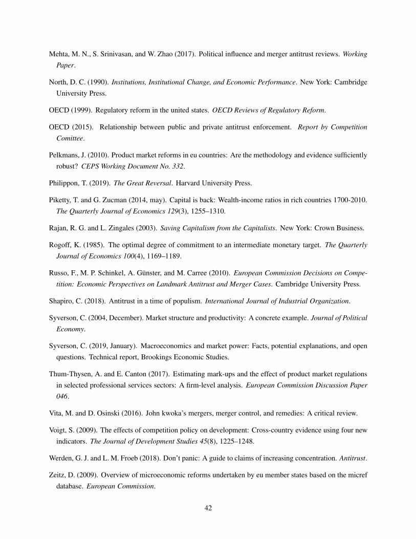
Mehta, M. N., S. Srinivasan, and W. Zhao (2017). Political influence and merger antitrust reviews. Working

Paper.

North, D. C. (1990). Institutions, Institutional Change, and Economic Performance. New York: Cambridge

University Press.

OECD (1999). Regulatory reform in the united states. OECD Reviews of Regulatory Reform.

OECD (2015). Relationship between public and private antitrust enforcement. Report by Competition

Comittee.

Pelkmans, J. (2010). Product market reforms in eu countries: Are the methodology and evidence sufficiently

robust? CEPS Working Document No. 332.

Philippon, T. (2019). The Great Reversal. Harvard University Press.

Piketty, T. and G. Zucman (2014, may). Capital is back: Wealth-income ratios in rich countries 1700-2010.

The Quarterly Journal of Economics 129(3), 1255–1310.

Rajan, R. G. and L. Zingales (2003). Saving Capitalism from the Capitalists. New York: Crown Business.

Rogoff, K. (1985). The optimal degree of commitment to an intermediate monetary target. The Quarterly

Journal of Economics 100(4), 1169–1189.

Russo, F., M. P. Schinkel, A. Günster, and M. Carree (2010). European Commission Decisions on Compe-

tition: Economic Perspectives on Landmark Antitrust and Merger Cases. Cambridge University Press.

Shapiro, C. (2018). Antitrust in a time of populism. International Journal of Industrial Organization.

Syverson, C. (2004, December). Market structure and productivity: A concrete example. Journal of Political

Economy.

Syverson, C. (2019, January). Macroeconomics and market power: Facts, potential explanations, and open

questions. Technical report, Brookings Economic Studies.

Thum-Thysen, A. and E. Canton (2017). Estimating mark-ups and the effect of product market regulations

in selected professional services sectors: A firm-level analysis. European Commission Discussion Paper

046.

Vita, M. and D. Osinski (2016). John kwoka’s mergers, merger control, and remedies: A critical review.

Voigt, S. (2009). The effects of competition policy on development: Cross-country evidence using four new

indicators. The Journal of Development Studies 45(8), 1225–1248.

Werden, G. J. and L. M. Froeb (2018). Don’t panic: A guide to claims of increasing concentration. Antitrust.

Zeitz, D. (2009). Overview of microeconomic reforms undertaken by eu member states based on the micref

database. European Commission.

42

Appendices: Not Intended for Publication

We provide one appendix for each main section of the paper, along with a Data Appendix.

• Appendix A focuses on US and EU competition measures

• Appendix B presents several model extensions

• Appendix C provides additional tests for prediction 1a: tougher and more independent regulator

• Appendix D provides additional tests for prediction 1b: Real Consequences

• Appendix E provides additional tests of prediction 2: Cross-Sectional Implications

• Appendix F provides a brief history of Antitrust and Regulatory Institutions on both Sides of the

Atlantic

• Appendix G describes our data sources and definitions

A Appendix: Evolution of Income Shares, Markups, and Concentration

Table 4 summarizes a wide range of measures of competition for the US and Europe. For each measure,

it reports the average value over two periods selected to avoid peaks and troughs in the economic cycle:

1997 to 1999 and 2013 to 2015. To facilitate comparison across measures, all results are based on the

non-agriculture business sector excluding Finance – except for concentration where we include Finance.34

As shown, virtually all measures remained stable in Europe yet deteriorated in the US. Investment rela-

tive to profits (I/GOS) declined in both regions – consistent with the rise of intangibles as emphasized in

Crouzet and Eberly (2018b) and Dottling et al. (2017) – but the decline is much larger in the US. In ad-

dition, estimates of the level and change in profits are broadly consistent between firm and industry-level

data. Take accounting profits, for example. Firm-level pretax income relative to sales increases from 7.5

to 8.5% in the US. Operating surplus to sales rises from 11.1% to 13.1%. In Europe, OS/PROD drops by

1.9%, while Pretax Income/Sales drops by 1.7%. Similarly, estimates of economic profits rise by similar

amounts. Average mark-ups adjusted for the cost of debt and equity (see below for definitions) increase by

2.2%. This implies an increase of 2.0% in profits relative to sales and 4.1% in profits relative to value added,

assuming a 50% intermediate input rate as in Basu (2019). The corresponding profit share of value added

increased by 5.6%. Similarly, for Europe, the average mark-ups rises from 101.3 to 102.1, which implies an

increase in profits/sale of 0.8% and an increase in profit share of 1.7%. The profit share based on industry

data decreased by 0.3%. The rest of this section provides additional details on the data sources, definitions

and results (including plots) underlying each row of the table.

34We exclude finance and non-business sectors due to difficulties in measuring the labor share and profits in industry data for

these sectors. See Gutiérrez and Piton (2019) for a discussion.

43

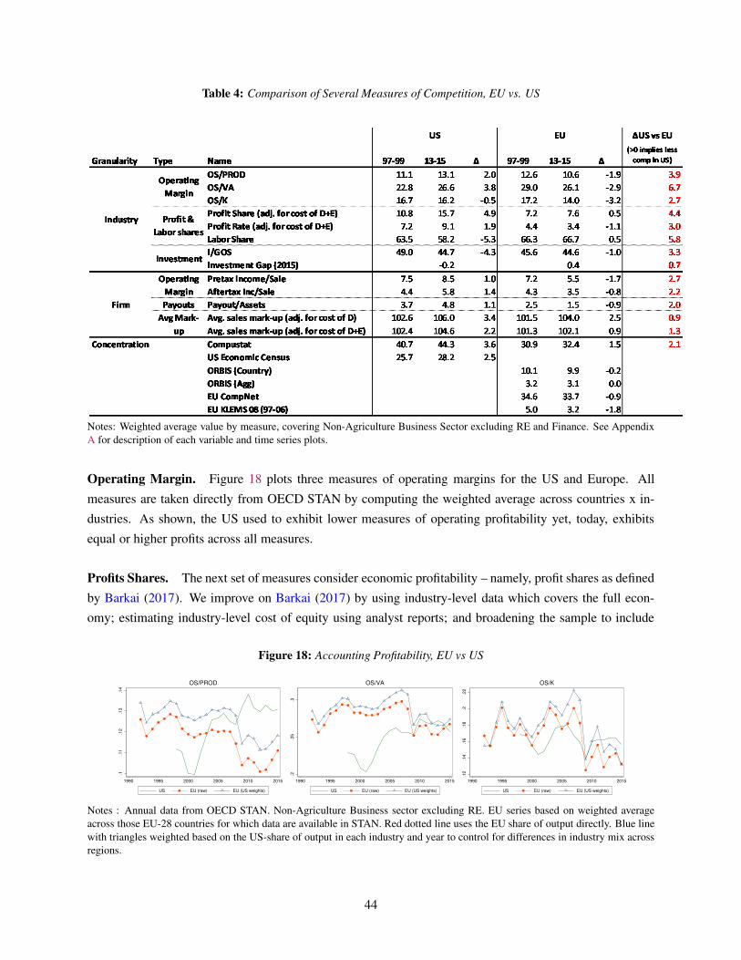
Table 4: Comparison of Several Measures of Competition, EU vs. US

Notes: Weighted average value by measure, covering Non-Agriculture Business Sector excluding RE and Finance. See Appendix

A for description of each variable and time series plots.

Operating Margin. Figure 18 plots three measures of operating margins for the US and Europe. All

measures are taken directly from OECD STAN by computing the weighted average across countries x in-

dustries. As shown, the US used to exhibit lower measures of operating profitability yet, today, exhibits

equal or higher profits across all measures.

Profits Shares. The next set of measures consider economic profitability – namely, profit shares as defined

by Barkai (2017). We improve on Barkai (2017) by using industry-level data which covers the full econ-

omy; estimating industry-level cost of equity using analyst reports; and broadening the sample to include

Figure 18: Accounting Profitability, EU vs US

.1.1

1.1

2.1

3.1

4

1990 1995 2000 2005 2010 2015

US EU (raw) EU (US weights)

OS/PROD

.2.2

5.3

1990 1995 2000 2005 2010 2015

US EU (raw) EU (US weights)

OS/VA

.12

.14

.16

.18

.2.2

2

1990 1995 2000 2005 2010 2015

US EU (raw) EU (US weights)

OS/K

Notes : Annual data from OECD STAN. Non-Agriculture Business sector excluding RE. EU series based on weighted average

across those EU-28 countries for which data are available in STAN. Red dotted line uses the EU share of output directly. Blue line

with triangles weighted based on the US-share of output in each industry and year to control for differences in industry mix across

regions.

44

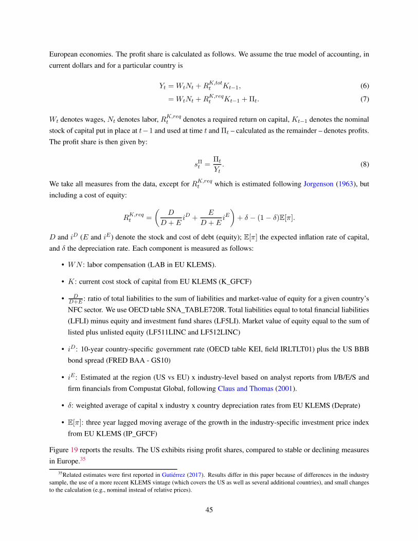
European economies. The profit share is calculated as follows. We assume the true model of accounting, in

current dollars and for a particular country is

Yt = WtNt +RK,tott Kt−1, (6)

= WtNt +RK,reqt Kt−1 +Πt. (7)

Wt denotes wages, Nt denotes labor, RK,reqt denotes a required return on capital, Kt−1 denotes the nominal

stock of capital put in place at t−1 and used at time t and Πt – calculated as the remainder – denotes profits.

The profit share is then given by:

sΠt =Πt

Yt. (8)

We take all measures from the data, except for RK,reqt which is estimated following Jorgenson (1963), but

including a cost of equity:

RK,reqt =

(

D

D + EiD +

E

D + EiE)

+ δ − (1− δ)E[π].

D and iD (E and iE) denote the stock and cost of debt (equity); E[π] the expected inflation rate of capital,

and δ the depreciation rate. Each component is measured as follows:

• WN : labor compensation (LAB in EU KLEMS).

• K: current cost stock of capital from EU KLEMS (K_GFCF)

• DD+E : ratio of total liabilities to the sum of liabilities and market-value of equity for a given country’s

NFC sector. We use OECD table SNA_TABLE720R. Total liabilities equal to total financial liabilities

(LFLI) minus equity and investment fund shares (LF5LI). Market value of equity equal to the sum of

listed plus unlisted equity (LF511LINC and LF512LINC)

• iD: 10-year country-specific government rate (OECD table KEI, field IRLTLT01) plus the US BBB

bond spread (FRED BAA - GS10)

• iE : Estimated at the region (US vs EU) x industry-level based on analyst reports from I/B/E/S and

firm financials from Compustat Global, following Claus and Thomas (2001).

• δ: weighted average of capital x industry x country depreciation rates from EU KLEMS (Deprate)

• E[π]: three year lagged moving average of the growth in the industry-specific investment price index

from EU KLEMS (IP_GFCF)

Figure 19 reports the results. The US exhibits rising profit shares, compared to stable or declining measures

in Europe.35

35Related estimates were first reported in Gutiérrez (2017). Results differ in this paper because of differences in the industry

sample, the use of a more recent KLEMS vintage (which covers the US as well as several additional countries), and small changes

to the calculation (e.g., nominal instead of relative prices).

45

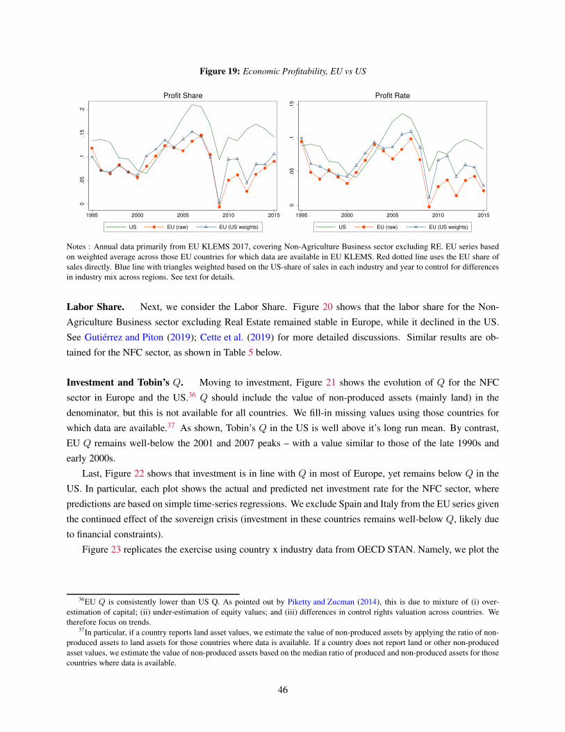
Figure 19: Economic Profitability, EU vs US0

.05

.1.1

5.2

1995 2000 2005 2010 2015

US EU (raw) EU (US weights)

Profit Share

0.0

5.1

.15

1995 2000 2005 2010 2015

US EU (raw) EU (US weights)

Profit Rate

Notes : Annual data primarily from EU KLEMS 2017, covering Non-Agriculture Business sector excluding RE. EU series based

on weighted average across those EU countries for which data are available in EU KLEMS. Red dotted line uses the EU share of

sales directly. Blue line with triangles weighted based on the US-share of sales in each industry and year to control for differences

in industry mix across regions. See text for details.

Labor Share. Next, we consider the Labor Share. Figure 20 shows that the labor share for the Non-

Agriculture Business sector excluding Real Estate remained stable in Europe, while it declined in the US.

See Gutiérrez and Piton (2019); Cette et al. (2019) for more detailed discussions. Similar results are ob-

tained for the NFC sector, as shown in Table 5 below.

Investment and Tobin’s Q. Moving to investment, Figure 21 shows the evolution of Q for the NFC

sector in Europe and the US.36 Q should include the value of non-produced assets (mainly land) in the

denominator, but this is not available for all countries. We fill-in missing values using those countries for

which data are available.37 As shown, Tobin’s Q in the US is well above it’s long run mean. By contrast,

EU Q remains well-below the 2001 and 2007 peaks – with a value similar to those of the late 1990s and

early 2000s.

Last, Figure 22 shows that investment is in line with Q in most of Europe, yet remains below Q in the

US. In particular, each plot shows the actual and predicted net investment rate for the NFC sector, where

predictions are based on simple time-series regressions. We exclude Spain and Italy from the EU series given

the continued effect of the sovereign crisis (investment in these countries remains well-below Q, likely due

to financial constraints).

Figure 23 replicates the exercise using country x industry data from OECD STAN. Namely, we plot the

36EU Q is consistently lower than US Q. As pointed out by Piketty and Zucman (2014), this is due to mixture of (i) over-

estimation of capital; (ii) under-estimation of equity values; and (iii) differences in control rights valuation across countries. We

therefore focus on trends.37In particular, if a country reports land asset values, we estimate the value of non-produced assets by applying the ratio of non-

produced assets to land assets for those countries where data is available. If a country does not report land or other non-produced

asset values, we estimate the value of non-produced assets based on the median ratio of produced and non-produced assets for those

countries where data is available.

46

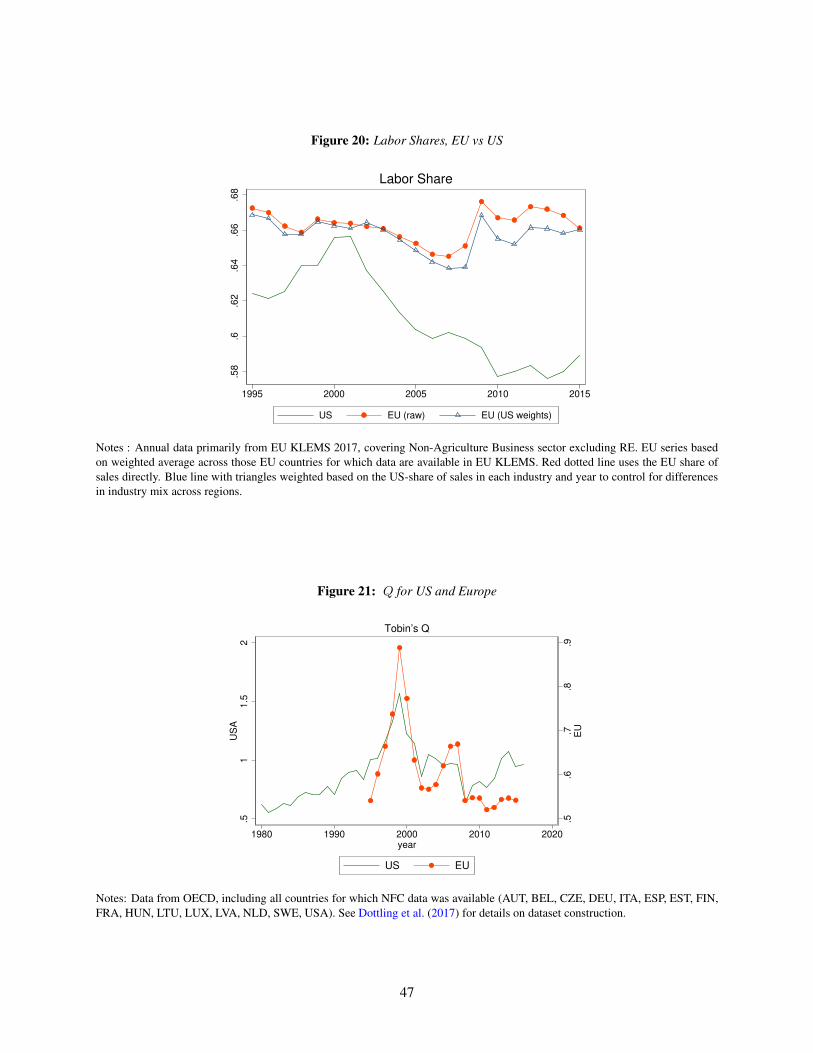
Figure 20: Labor Shares, EU vs US

.58

.6.6

2.6

4.6

6.6

8

1995 2000 2005 2010 2015

US EU (raw) EU (US weights)

Labor Share

Notes : Annual data primarily from EU KLEMS 2017, covering Non-Agriculture Business sector excluding RE. EU series based

on weighted average across those EU countries for which data are available in EU KLEMS. Red dotted line uses the EU share of

sales directly. Blue line with triangles weighted based on the US-share of sales in each industry and year to control for differences

in industry mix across regions.

Figure 21: Q for US and Europe

.5.6

.7.8

.9E

U

.51

1.5

2U

SA

1980 1990 2000 2010 2020year

US EU

Tobin’s Q

Notes: Data from OECD, including all countries for which NFC data was available (AUT, BEL, CZE, DEU, ITA, ESP, EST, FIN,

FRA, HUN, LTU, LUX, LVA, NLD, SWE, USA). See Dottling et al. (2017) for details on dataset construction.

47

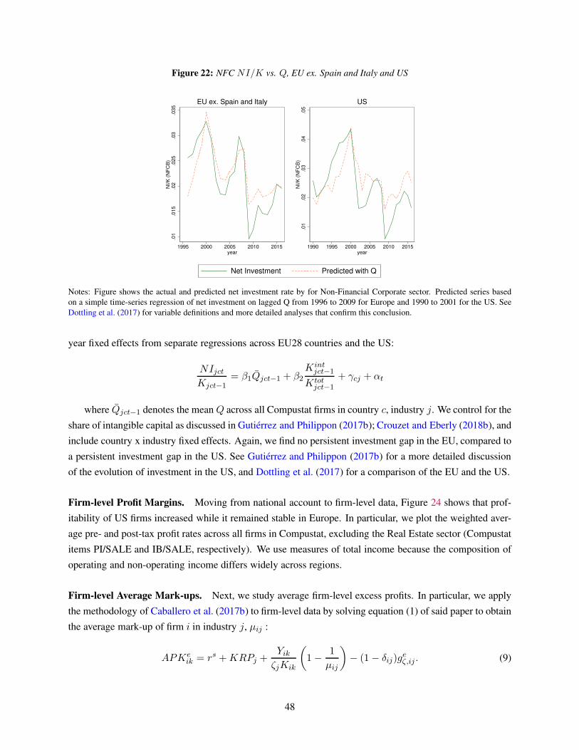
Figure 22: NFC NI/K vs. Q, EU ex. Spain and Italy and US

.01

.01

5.0

2.0

25

.03

.03

5N

I/K

(N

FC

B)

1995 2000 2005 2010 2015year

EU ex. Spain and Italy

.01

.02

.03

.04

.05

NI/

K (

NF

CB

)

1990 1995 2000 2005 2010 2015year

US

Net Investment Predicted with Q

Notes: Figure shows the actual and predicted net investment rate by for Non-Financial Corporate sector. Predicted series based

on a simple time-series regression of net investment on lagged Q from 1996 to 2009 for Europe and 1990 to 2001 for the US. See

Dottling et al. (2017) for variable definitions and more detailed analyses that confirm this conclusion.

year fixed effects from separate regressions across EU28 countries and the US:

NIjctKjct−1

= β1Qjct−1 + β2Kint

jct−1

Ktotjct−1

+ γcj + αt

where Qjct−1 denotes the mean Q across all Compustat firms in country c, industry j. We control for the

share of intangible capital as discussed in Gutiérrez and Philippon (2017b); Crouzet and Eberly (2018b), and

include country x industry fixed effects. Again, we find no persistent investment gap in the EU, compared to

a persistent investment gap in the US. See Gutiérrez and Philippon (2017b) for a more detailed discussion

of the evolution of investment in the US, and Dottling et al. (2017) for a comparison of the EU and the US.

Firm-level Profit Margins. Moving from national account to firm-level data, Figure 24 shows that prof-

itability of US firms increased while it remained stable in Europe. In particular, we plot the weighted aver-

age pre- and post-tax profit rates across all firms in Compustat, excluding the Real Estate sector (Compustat

items PI/SALE and IB/SALE, respectively). We use measures of total income because the composition of

operating and non-operating income differs widely across regions.

Firm-level Average Mark-ups. Next, we study average firm-level excess profits. In particular, we apply

the methodology of Caballero et al. (2017b) to firm-level data by solving equation (1) of said paper to obtain

the average mark-up of firm i in industry j, µij :

APKeik = rs +KRPj +

Yik

ζjKik

(

1− 1

µij

)

− (1− δij)geζ,ij . (9)

48

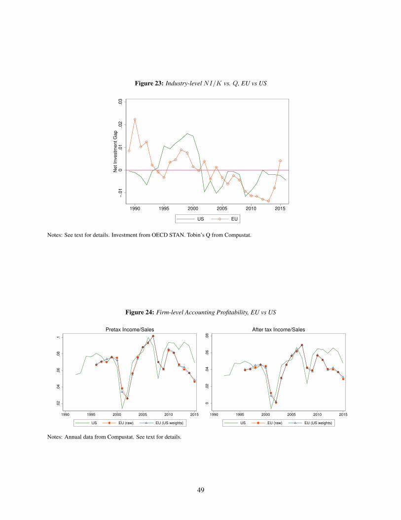
Figure 23: Industry-level NI/K vs. Q, EU vs US

−.0

10

.01

.02

.03

Net In

vestm

ent G

ap

1990 1995 2000 2005 2010 2015

US EU

Notes: See text for details. Investment from OECD STAN. Tobin’s Q from Compustat.

Figure 24: Firm-level Accounting Profitability, EU vs US

.02

.04

.06

.08

.1

1990 1995 2000 2005 2010 2015

US EU (raw) EU (US weights)

Pretax Income/Sales

0.0

2.0

4.0

6.0

8

1990 1995 2000 2005 2010 2015

US EU (raw) EU (US weights)

After tax Income/Sales

Notes: Annual data from Compustat. See text for details.

49

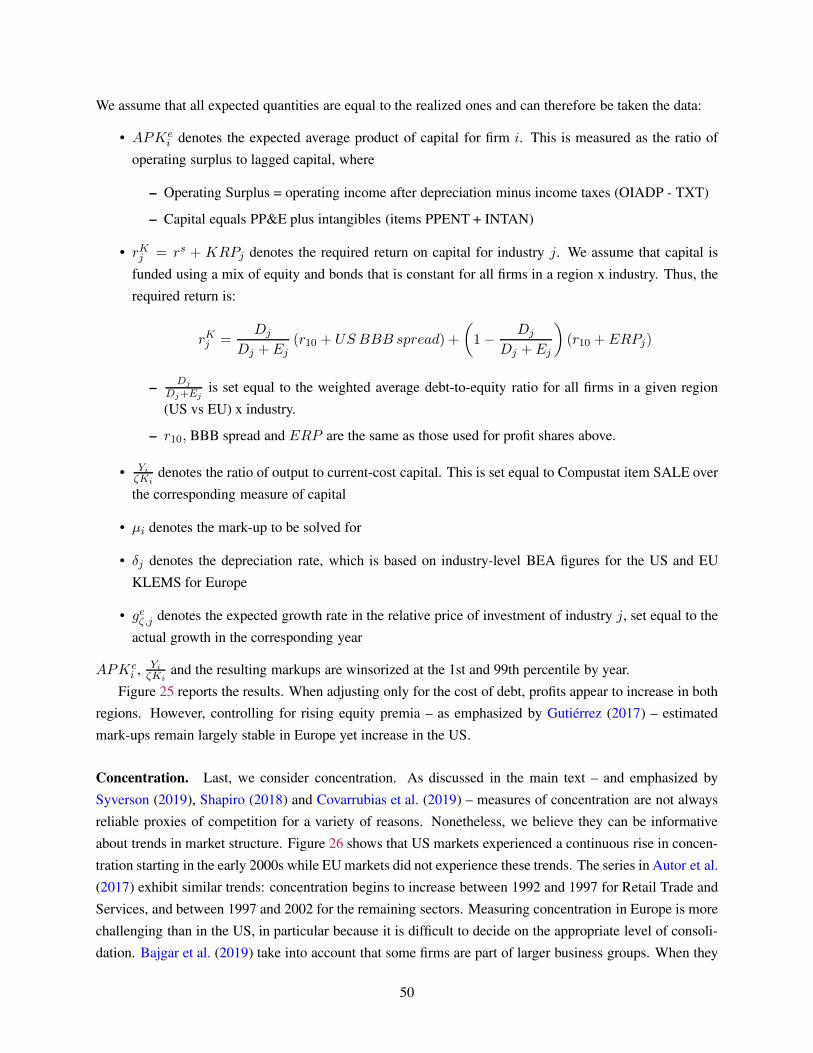
We assume that all expected quantities are equal to the realized ones and can therefore be taken the data:

• APKei denotes the expected average product of capital for firm i. This is measured as the ratio of

operating surplus to lagged capital, where

– Operating Surplus = operating income after depreciation minus income taxes (OIADP - TXT)

– Capital equals PP&E plus intangibles (items PPENT + INTAN)

• rKj = rs + KRPj denotes the required return on capital for industry j. We assume that capital is

funded using a mix of equity and bonds that is constant for all firms in a region x industry. Thus, the

required return is:

rKj =Dj

Dj + Ej(r10 + US BBB spread) +

(

1− Dj

Dj + Ej

)

(r10 + ERPj)

–Dj

Dj+Ejis set equal to the weighted average debt-to-equity ratio for all firms in a given region

(US vs EU) x industry.

– r10, BBB spread and ERP are the same as those used for profit shares above.

• Yi

ζKidenotes the ratio of output to current-cost capital. This is set equal to Compustat item SALE over

the corresponding measure of capital

• µi denotes the mark-up to be solved for

• δj denotes the depreciation rate, which is based on industry-level BEA figures for the US and EU

KLEMS for Europe

• geζ,j denotes the expected growth rate in the relative price of investment of industry j, set equal to the

actual growth in the corresponding year

APKei , Yi

ζKiand the resulting markups are winsorized at the 1st and 99th percentile by year.

Figure 25 reports the results. When adjusting only for the cost of debt, profits appear to increase in both

regions. However, controlling for rising equity premia – as emphasized by Gutiérrez (2017) – estimated

mark-ups remain largely stable in Europe yet increase in the US.

Concentration. Last, we consider concentration. As discussed in the main text – and emphasized by

Syverson (2019), Shapiro (2018) and Covarrubias et al. (2019) – measures of concentration are not always

reliable proxies of competition for a variety of reasons. Nonetheless, we believe they can be informative

about trends in market structure. Figure 26 shows that US markets experienced a continuous rise in concen-

tration starting in the early 2000s while EU markets did not experience these trends. The series in Autor et al.

(2017) exhibit similar trends: concentration begins to increase between 1992 and 1997 for Retail Trade and

Services, and between 1997 and 2002 for the remaining sectors. Measuring concentration in Europe is more

challenging than in the US, in particular because it is difficult to decide on the appropriate level of consoli-

dation. Bajgar et al. (2019) take into account that some firms are part of larger business groups. When they

50

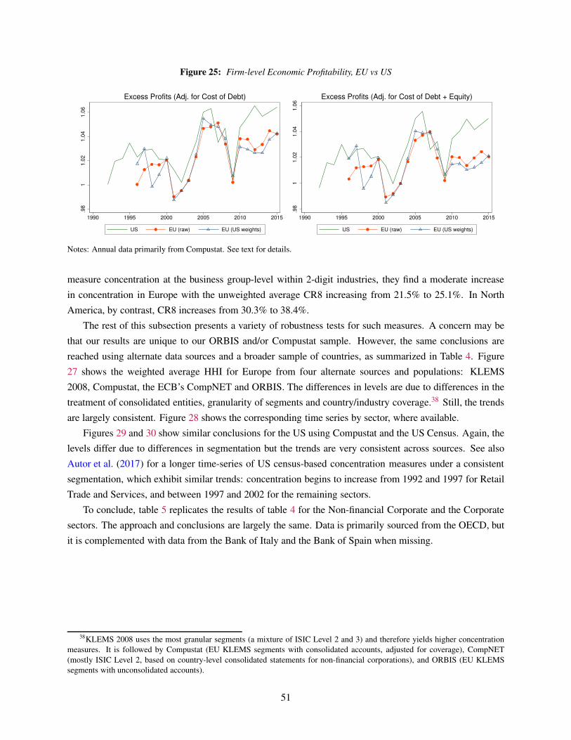
Figure 25: Firm-level Economic Profitability, EU vs US.9

81

1.0

21.0

41.0

6

1990 1995 2000 2005 2010 2015

US EU (raw) EU (US weights)

Excess Profits (Adj. for Cost of Debt)

.98

11.0

21.0

41.0

6

1990 1995 2000 2005 2010 2015

US EU (raw) EU (US weights)

Excess Profits (Adj. for Cost of Debt + Equity)

Notes: Annual data primarily from Compustat. See text for details.

measure concentration at the business group-level within 2-digit industries, they find a moderate increase

in concentration in Europe with the unweighted average CR8 increasing from 21.5% to 25.1%. In North

America, by contrast, CR8 increases from 30.3% to 38.4%.

The rest of this subsection presents a variety of robustness tests for such measures. A concern may be

that our results are unique to our ORBIS and/or Compustat sample. However, the same conclusions are

reached using alternate data sources and a broader sample of countries, as summarized in Table 4. Figure

27 shows the weighted average HHI for Europe from four alternate sources and populations: KLEMS

2008, Compustat, the ECB’s CompNET and ORBIS. The differences in levels are due to differences in the

treatment of consolidated entities, granularity of segments and country/industry coverage.38 Still, the trends

are largely consistent. Figure 28 shows the corresponding time series by sector, where available.

Figures 29 and 30 show similar conclusions for the US using Compustat and the US Census. Again, the

levels differ due to differences in segmentation but the trends are very consistent across sources. See also

Autor et al. (2017) for a longer time-series of US census-based concentration measures under a consistent

segmentation, which exhibit similar trends: concentration begins to increase from 1992 and 1997 for Retail

Trade and Services, and between 1997 and 2002 for the remaining sectors.

To conclude, table 5 replicates the results of table 4 for the Non-financial Corporate and the Corporate

sectors. The approach and conclusions are largely the same. Data is primarily sourced from the OECD, but

it is complemented with data from the Bank of Italy and the Bank of Spain when missing.

38KLEMS 2008 uses the most granular segments (a mixture of ISIC Level 2 and 3) and therefore yields higher concentration

measures. It is followed by Compustat (EU KLEMS segments with consolidated accounts, adjusted for coverage), CompNET

(mostly ISIC Level 2, based on country-level consolidated statements for non-financial corporations), and ORBIS (EU KLEMS

segments with unconsolidated accounts).

51

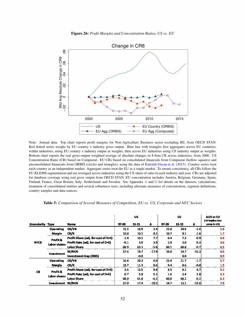
Figure 26: Profit Margins and Concentration Ratios, US vs. EU

−.0

20

.02

.04

.06

.08

Wtd

Avg A

bsolu

te C

hange in C

R8

2000 2005 2010 2015

US EU Country (ORBIS)

EU Agg (ORBIS) EU Agg (Compustat)

Change in CR8

Note: Annual data. Top chart reports profit margins for Non-Agriculture Business sector excluding RE, from OECD STAN.

Red dotted series weighs by EU country x industry gross output. Blue line with triangles first aggregates across EU countries,

within industries, using EU country x industry output as weights, then across EU industries using US industry output as weights.

Bottom chart reports the real gross-output weighted average of absolute changes in 8-firm CR across industries, from 2000. US

Concentration Ratio (CR) based on Compustat. EU CRs based on consolidated financials from Compustat (hollow squares) and

unconsolidated financials from ORBIS (circles and triangles), using the data of Kalemli-Ozcan et al. (2015). Country series treat

each country as an independent market. Aggregate series treat the EU as a single market. To ensure consistency, all CRs follow the

EU KLEMS segmentation and are averaged across industries using the US-share of sales in each industry and year. CRs are adjusted

for database coverage using real gross output from OECD STAN. EU concentration includes Austria, Belgium, Germany, Spain,

Finland, France, Great Britain, Italy, Netherlands and Sweden. See Appendix A and G for details on the datasets, calculations,

treatment of consolidated entities and several robustness tests, including alternate measures of concentration, segment definitions,

country samples and data sources.

Table 5: Comparison of Several Measures of Competition, EU vs. US, Corporate and NFC Sectors

52

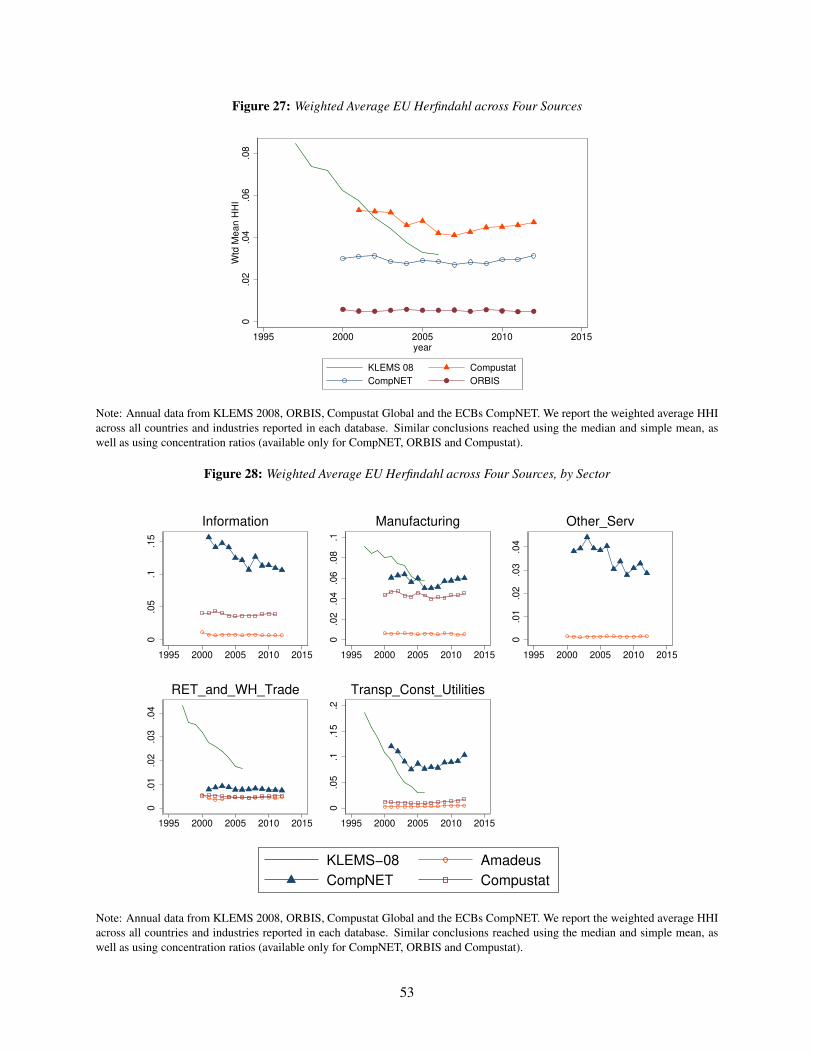
Figure 27: Weighted Average EU Herfindahl across Four Sources

0.0

2.0

4.0

6.0

8W

td M

ean H

HI

1995 2000 2005 2010 2015year

KLEMS 08 Compustat

CompNET ORBIS

Note: Annual data from KLEMS 2008, ORBIS, Compustat Global and the ECBs CompNET. We report the weighted average HHI

across all countries and industries reported in each database. Similar conclusions reached using the median and simple mean, as

well as using concentration ratios (available only for CompNET, ORBIS and Compustat).

Figure 28: Weighted Average EU Herfindahl across Four Sources, by Sector

0.0

5.1

.15

1995 2000 2005 2010 2015

Information

0.0

2.0

4.0

6.0

8.1

1995 2000 2005 2010 2015

Manufacturing0

.01

.02

.03

.04

1995 2000 2005 2010 2015

Other_Serv

0.0

1.0

2.0

3.0

4

1995 2000 2005 2010 2015

RET_and_WH_Trade

0.0

5.1

.15

.2

1995 2000 2005 2010 2015

Transp_Const_Utilities

KLEMS−08 Amadeus

CompNET Compustat

Note: Annual data from KLEMS 2008, ORBIS, Compustat Global and the ECBs CompNET. We report the weighted average HHI

across all countries and industries reported in each database. Similar conclusions reached using the median and simple mean, as

well as using concentration ratios (available only for CompNET, ORBIS and Compustat).

53

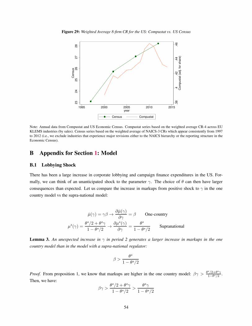
Figure 29: Weighted Average 8-firm CR for the US: Compustat vs. US Census

.38

.4.4

2.4

4.4

6C

om

pusta

t (a

dj. for

share

)

23

24

25

26

27

28

Census

1995 2000 2005 2010 2015year

Census Compustat

Note: Annual data from Compustat and US Economic Census. Compustat series based on the weighted average CR-4 across EU

KLEMS industries (by sales). Census series based on the weighted average of NAICS-3 CRs which appear consistently from 1997

to 2012 (i.e., we exclude industries that experience major revisions either to the NAICS hierarchy or the reporting structure in the

Economic Census).

B Appendix for Section 1: Model

B.1 Lobbying Shock

There has been a large increase in corporate lobbying and campaign finance expenditures in the US. For-

mally, we can think of an unanticipated shock to the parameter γ. The choice of θ can then have larger

consequences than expected. Let us compare the increase in markups from positive shock to γ in the one

country model vs the supra-national model:

µ(γ) = γβ → ∂µ(γ)

∂γ= β One-country

µs(γ) =θs/2 + θsγ

1− θs/2→ ∂µs(γ)

∂γ=

θs

1− θs/2Supranational

Lemma 3. An unexpected increase in γ in period 2 generates a larger increase in markups in the one

country model than in the model with a supra-national regulator:

β >θs

1− θs/2

Proof. From proposition 1, we know that markups are higher in the one country model: βγ > θs/2+θsγ1−θs/2 .

Then, we have:

βγ >θs/2 + θsγ

1− θs/2>

θsγ

1− θs/2

54

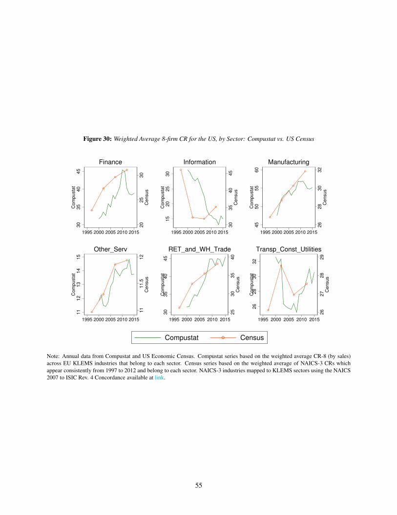
Figure 30: Weighted Average 8-firm CR for the US, by Sector: Compustat vs. US Census2

02

53

0C

en

su

s

30

35

40

45

Co

mp

usta

t

1995 2000 2005 2010 2015

Finance

30

35

40

45

Ce

nsu

s

15

20

25

30

Co

mp

usta

t

1995 2000 2005 2010 2015

Information

26

28

30

32

Ce

nsu

s

45

50

55

60

Co

mp

usta

t

1995 2000 2005 2010 2015

Manufacturing

11

11

.51

2C

en

su

s

11

12

13

14

15

Co

mp

usta

t

1995 2000 2005 2010 2015

Other_Serv

25

30

35

40

Ce

nsu

s

30

35

40

45

Co

mp

usta

t

1995 2000 2005 2010 2015

RET_and_WH_Trade

26

27

28

29

Ce

nsu

s

26

28

30

32

Co

mp

usta

t

1995 2000 2005 2010 2015

Transp_Const_Utilities

Compustat Census

Note: Annual data from Compustat and US Economic Census. Compustat series based on the weighted average CR-8 (by sales)

across EU KLEMS industries that belong to each sector. Census series based on the weighted average of NAICS-3 CRs which

appear consistently from 1997 to 2012 and belong to each sector. NAICS-3 industries mapped to KLEMS sectors using the NAICS

2007 to ISIC Rev. 4 Concordance available at link.

55

Dividing by γ, we get β > θs

1−θs/2 .

B.2 General Utility

As in the logarithmic case, since firms in industry i cannot set a markup higher than µi, firms choose the

maximum price pi = (1 + µi)w/zi. Given prices and wages, household maximize

U = max

2∑

i=1

u (xi)− n

s.t.

2∑

i=1

pixi = wn+

2∑

i=1

Π$i

where Π$i are nominal profits from industry i. Let λ be the Lagrange multiplier on the budget constraint.

We have u′ (xi) = λpi and 1 = λw. Using the equation for price, we then get u′ (xi) = 1 + µi. So

there is simple direct mapping between the markups and the quantities produced in equilibrium. We can

therefore think of the regulator as indirectly choosing the quantities {xi}i=1,2. This leads to the indirect

utility function for the households

U ({xi}i) =2∑

i=1

u (xi)− xi/zi

Real Profits (nominal profits divided by wage) are

Πi ≡ xipi/w − xi/zi = µ (xi)xi/zi

Note that∂Π

∂xi(x⋆) < 0

This is simply because µ (x⋆) = 0 and∂µ(xi)∂xi

< 0. We assume for convenience that ∂π∂xi

< 0 for the relevant

range of values.39

Welfare and Capture Ex-Post With general utility, the problem of the regulator is:

max{xi}

U ({xi}i) + θγΠǫ

Let us define xǫ as the solution to

u′ (xǫ) ≡ 1/zi − θγΠ′ (xǫ)

39For instance, if u ≡ log, then x⋆ = 1 and πi (xi) = 1− xi.

56

Lemma 4. The equilibrium under regulation is

xi (i = ǫ) = xǫ

xi (i 6= ǫ) = x⋆

where xǫ < x⋆. The indirect utility is

U (ǫ, θ) = U (θ) = u (x⋆)− x⋆/zǫ 6=i + u (xǫ)− xǫ/zǫ=i

and profits are positive if ǫ = i and zero otherwise.

Proof. The regulator sets markup limits to maximize

2∑

i=1

u (xi)− xi/zi + θγΠ(xi=ǫ)

The first order conditions are then

u′ (xi) = 1/zi − θγΠ′ (xi) 1i=ǫ

and xǫ < x⋆ since π′ (x⋆) < 0.

Note that, because of symmetry, U (ǫ, θ) does not actually depend on whether ǫ = 1 or ǫ = 2.

Ex-ante Design of Regulatory Independence. This part of the problem is unaffected by the specification

of the utility function and in particular we still have that politicians at design stage would set θ = β where

β captures the bias of the politician.

Supra-national Regulatory Design. Now we extend our model to two countries with specialized produc-

tion. Again, by law of one price and balance of trade, we have that wi = wj and xij = xii = xi. By market

clearing, we have that zini = xij + xji = 2xi, so

ni =2xizi

Then, we can write the indirect utility of consumers in country i as

Ui({xi}i) = u(xi) + u(xj)−(

2xizi

)1/α

Lets call profits under the supra-national regulator Πs. Real profits of the firm are

Πsi (µ) = 2µ(xi)xi/zi

Thus, compared with profits in the one country model, we have Πs = 2Π. The objective of the regulator is

57

R = max{xi}

Ui=ǫ + (1− θ)Ui 6=ǫ + θγΠsi=ǫ

=max(2− θ)u(xi=ǫ) + (2− θ)u(xi 6=ǫ)−2xi=ǫ

zi=ǫ− (1− θ)

2xi 6=ǫ

zi 6=ǫ+ θγΠs

i=ǫ

The first order condition for xi=ǫ is:

(2− θ)u′(xi=ǫ) = 2/zi=ǫ + θγΠ′s(xi=ǫ) = 2[1/zi=ǫ + θγΠ′(xi=ǫ)]

In order to compare to the first order condition in the one country model, Lets call the solution to

this equation xsi=ǫ and the solution in the one country model xi=ǫ. For the one country model, we had

u′ (xi) = 1/zi−θγΠ′ (x) 1ǫ=i. Then, we have that u′(xsi=ǫ) =2

2−θu′(xi=ǫ), which implies that xsi=ǫ < xi=ǫ

as in the case with logarithmic preferences.

For xi 6=ǫ, the first order condition is

(2− θ)u′(xi 6=ǫ) = 2(1− θ)/zi 6=ǫ

Again, comparing the first order condition its easy to see that xsi 6=ǫ > xi 6=ǫ, so we have that with general

utility the problem of the supra-national regulator has the same distortions with respect to the one-country

problem than in the logarithmic case.

B.3 Decreasing Returns

We consider the case where the production function is

xi = zinαi

Now the real profits of the firm are Πi ≡ π (xi) = xipi/w− (xi/zi)1/α. Thus, calculating the marginal cost

and using the definition of markups we get

pi =1 + µi

zi

w

α

(

xizi

)1−αα

The consumption problem is the same as before, so w/pi = xi. Replacing and solving for xi we get

xi = αα zi1 + µi

Thus, the regulator is indirectly choosing xi, and the welfare maximizing quantity is x∗ = ααzi.

Welfare and capture ex-post. The politicians maximize V (ǫ) = U + γΠǫ. Since they have influence θ

over the regulator, the regulator maximizes

R = max{xi}

(1− θ)U + θV (ǫ) = U({xi}i) + γθΠǫ

58

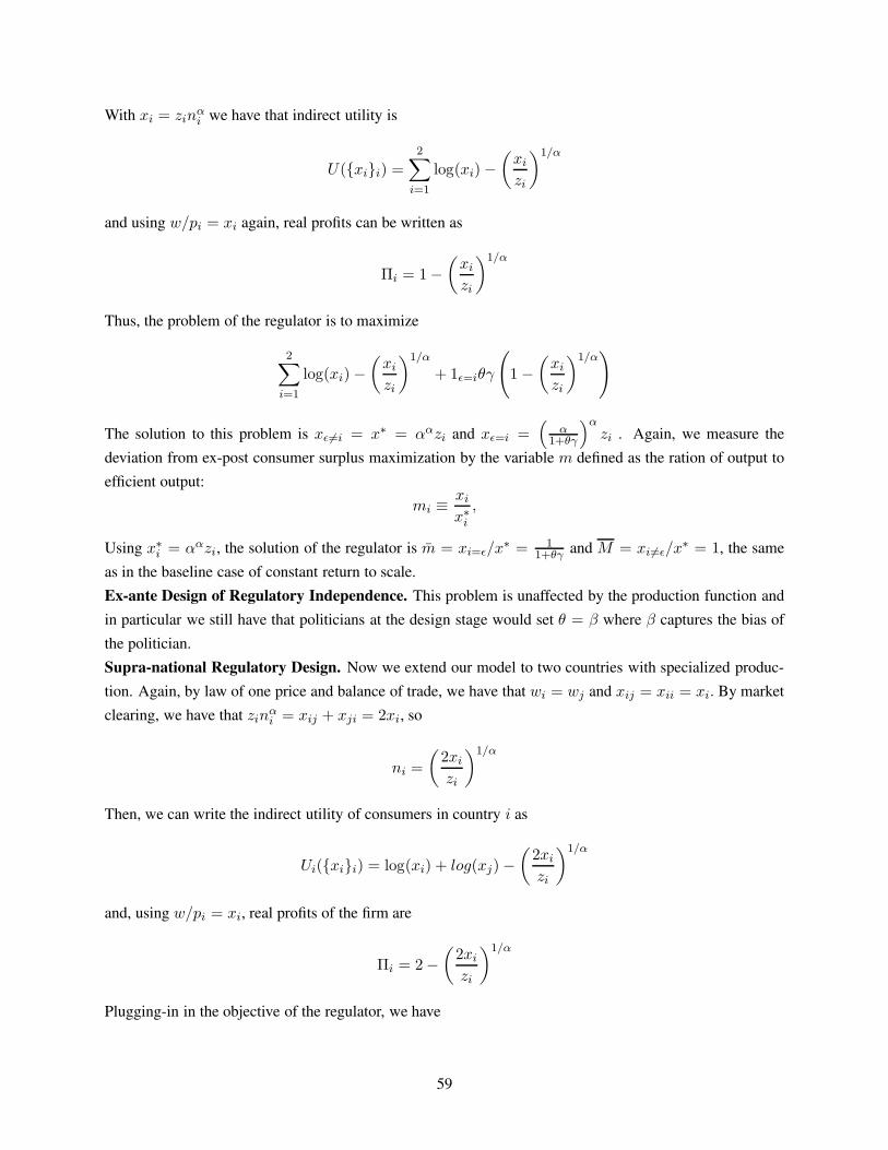
With xi = zinαi we have that indirect utility is

U({xi}i) =2∑

i=1

log(xi)−(

xizi

)1/α

and using w/pi = xi again, real profits can be written as

Πi = 1−(

xizi

)1/α

Thus, the problem of the regulator is to maximize

2∑

i=1

log(xi)−(

xizi

)1/α

+ 1ǫ=iθγ

(

1−(

xizi

)1/α)

The solution to this problem is xǫ 6=i = x∗ = ααzi and xǫ=i =(

α1+θγ

)αzi . Again, we measure the

deviation from ex-post consumer surplus maximization by the variable m defined as the ration of output to

efficient output:

mi ≡xix∗i

,

Using x∗i = ααzi, the solution of the regulator is m = xi=ǫ/x∗ = 1

1+θγ and M = xi 6=ǫ/x∗ = 1, the same

as in the baseline case of constant return to scale.

Ex-ante Design of Regulatory Independence. This problem is unaffected by the production function and

in particular we still have that politicians at the design stage would set θ = β where β captures the bias of

the politician.

Supra-national Regulatory Design. Now we extend our model to two countries with specialized produc-

tion. Again, by law of one price and balance of trade, we have that wi = wj and xij = xii = xi. By market

clearing, we have that zinαi = xij + xji = 2xi, so

ni =

(

2xizi

)1/α

Then, we can write the indirect utility of consumers in country i as

Ui({xi}i) = log(xi) + log(xj)−(

2xizi

)1/α

and, using w/pi = xi, real profits of the firm are

Πi = 2−(

2xizi

)1/α

Plugging-in in the objective of the regulator, we have

59

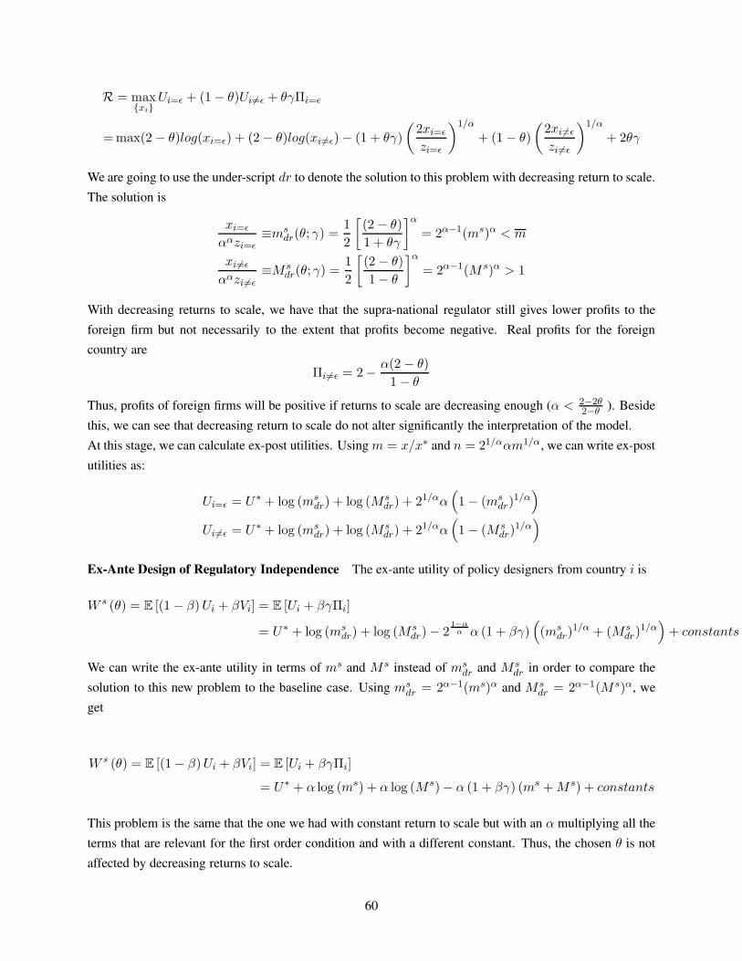
R = max{xi}

Ui=ǫ + (1− θ)Ui 6=ǫ + θγΠi=ǫ

=max(2− θ)log(xi=ǫ) + (2− θ)log(xi 6=ǫ)− (1 + θγ)

(

2xi=ǫ

zi=ǫ

)1/α

+ (1− θ)

(

2xi 6=ǫ

zi 6=ǫ

)1/α

+ 2θγ

We are going to use the under-script dr to denote the solution to this problem with decreasing return to scale.

The solution is

xi=ǫ

ααzi=ǫ≡ms

dr(θ; γ) =1

2

[

(2− θ)

1 + θγ

]α

= 2α−1(ms)α < m

xi 6=ǫ

ααzi 6=ǫ≡M s

dr(θ; γ) =1

2

[

(2− θ)

1− θ

]α

= 2α−1(M s)α > 1

With decreasing returns to scale, we have that the supra-national regulator still gives lower profits to the

foreign firm but not necessarily to the extent that profits become negative. Real profits for the foreign

country are

Πi 6=ǫ = 2− α(2 − θ)

1− θ

Thus, profits of foreign firms will be positive if returns to scale are decreasing enough (α < 2−2θ2−θ ). Beside

this, we can see that decreasing return to scale do not alter significantly the interpretation of the model.

At this stage, we can calculate ex-post utilities. Using m = x/x∗ and n = 21/ααm1/α, we can write ex-post

utilities as:

Ui=ǫ = U∗ + log (msdr) + log (M s

dr) + 21/αα(

1− (msdr)

1/α)

Ui 6=ǫ = U∗ + log (msdr) + log (M s

dr) + 21/αα(

1− (M sdr)

1/α)

Ex-Ante Design of Regulatory Independence The ex-ante utility of policy designers from country i is

W s (θ) = E [(1− β)Ui + βVi] = E [Ui + βγΠi]

= U∗ + log (msdr) + log (M s

dr)− 21−αα α (1 + βγ)

(

(msdr)

1/α + (M sdr)

1/α)

+ constants

We can write the ex-ante utility in terms of ms and M s instead of msdr and M s

dr in order to compare the

solution to this new problem to the baseline case. Using msdr = 2α−1(ms)α and M s

dr = 2α−1(M s)α, we

get

W s (θ) = E [(1− β)Ui + βVi] = E [Ui + βγΠi]

= U∗ + α log (ms) + α log (M s)− α (1 + βγ) (ms +M s) + constants

This problem is the same that the one we had with constant return to scale but with an α multiplying all the

terms that are relevant for the first order condition and with a different constant. Thus, the chosen θ is not

affected by decreasing returns to scale.

60

B.4 Externality

In the main text we assume that the designers are politicians, and as such they are biased. We can also

consider an externality to create a meaningful tension between the first best and the decentralized equilibrium

under perfect competition. We assume that aggregate welfare is the sum of households’ direct utility from

consumption and leisure plus a term that increases with industry profits

W = U + αΠη

where η = 1, 2 with equal probability. The term αΠη can have several interpretations, from innova-

tion, increasing returns, and financial distress to political economy. For instance, it is similar to that in

Lim and Yurukoglu (2018).40 Without this externality, it would be trivially optimal to delegate control to

a completely independent regulator tasked with enforcing perfect competition. With the externality, on the

other hand, there is room for a politician to make a legitimate case for protecting an industry. We introduce

randomness (via η) to create value for flexibility, i.e., it is not known in advance which industry really needs

some (temporary) protection. Of course, politicians have their own agendas and full flexibility is not optimal

either. We define

ζ ≡ Pr (ǫ = η) .

The parameter ζ denotes the congruence between public interest and politicians’ preference ex-post. When

ζ = 1, politicians always care about the industry that needs protection. When ζ < 1, they sometimes care

about the industry that does not need protection. Aggregate welfare is

W (ǫ, η; θ) = U (θ) + α1η=ǫπ (mθ) .

The founding fathers choose θ to maximize

V0 = maxθ

E [W (ǫ, η; θ)] = U (θ) + αζπ (mθ)

It is easy to see that the optimal choice is to set θγ = αζ .

Lemma 5. In a closed economy (one country), the politicians choose a regulatory framework with influence

parameter

θ =α

γζ

This model is formally equivalent to the model we have used so far if we set β = αγ ζ .

40There are several ways to motivate this externality. One is a model of financial distress and inefficient liquidation, where it

can be optimal to help an industry, for instance during a financial crisis. Another is a model with incentives to innovate or to invest.

Lim and Yurukoglu (2018) study a dynamic investment game between an electricity firm and a regulator subject to time consistency

issues, where the regulator puts a weight on customer surplus and a weight on the firm’s profits. There is also a political economy

interpretation. A government implementing difficult reforms needs to pick its fights carefully. For instance, in France, the national

railway company arguably suffers from excessive prices (and wages) but also from excessive pension obligations. It may be too

risky to implement the pension reform and the deregulation of services at the same time, however. The exact nature and shape of

the externality is not important for our results, as long as it is an increasing function of industry profits.

61

B.5 N Countries

We can also extend our analysis to the case of N countries and N goods. For simplicity we normalize the

z′is to 1. Indirect utilities are given by

Ui =N∑

j=1

log (xj)−Nxi

and profits are

Πi = N (1− xi)

The regulator therefore maximizes

max{µ}

(1− θ)

N∑

i=1

Ui + θVǫ

With probability 1/N , country 1 gets to influence the regulator. In that case, the regulator solves

max{µ}

U1 + (1− θ)

N∑

j=2

Uj + θγΠ1

This is equivalent to maximizing

(1 + (N − 1) (1− θ))N∑

j=1

log (xj)−Nx1 −N (1− θ)N∑

j=2

xj +Nθγ (1− x1)

The solution is

x1 (ǫ = 1) = mNθ =

1− N−1N θ

1 + θγ

xj (ǫ = 1) = MNθ =

1− N−1N θ

1− θ

Country 1’s favorite choice of θ at the design stage maximizes

E [U1 (ǫ, θ) + βΠ1 (ǫ, θ)] =1

N

(

log(

mNθ

)

+ (N − 1) log(

MNθ

)

−NmNθ +Nβ

(

1−mNθ

))

+N − 1

N

(

log(

mNθ

)

+ (N −

= log(

mNθ

)

+ (N − 1) log(

MNθ

)

− (1 + β)mNθ − (N − 1) (1 + β)Mθ +Nβ

If we abstract first from regulatory over-reach by keeping MNθ constant, we see that the optimal choice of

mNθ would be again 1

1+β . From the functional form of mNθ this requires increasing independence as N

increases θ(N) = β

γ+(1+β)N−1

N

.

If we consider now the full problem, including regulatory over-reach, we see that M is a strictly increas-

ing function of θ. We can thus write M (m) as a decreasing function and use m as a choice variable. The

62

first order condition is1

m= 1 + β + (N − 1)

∂M

∂m

(

1 + β − 1

M

)

Since M > 1, ∂M∂m

(

1 + β − 1M

)

< 0 and therefore m is larger than (1 + β)−1. This proves θ(N) < θ. We

have∂ logm

∂θ=

−γ

1 + γθ−

N−1N

1− N−1N θ

and∂ logM

∂θ=

1

1− θ−

N−1N

1− N−1N θ

When θ = 0 and m = M = 1, we have ∂M∂θ = 1

N ; ∂m∂θ = −γ − N−1N therefore

∂M

∂m(1) = − 1

Nγ +N − 1

Thus if we estimate at m = M = 1,

1 + β + (N − 1) β∂M

∂m(1) = 1 + β

(

γ

γ + N−1N

)

> 1

Thus θ(N) > 0 but decreasing in N . In the limit of large N , we get a finite slope β(

γγ+1

)

starting from the

efficient allocation.

63

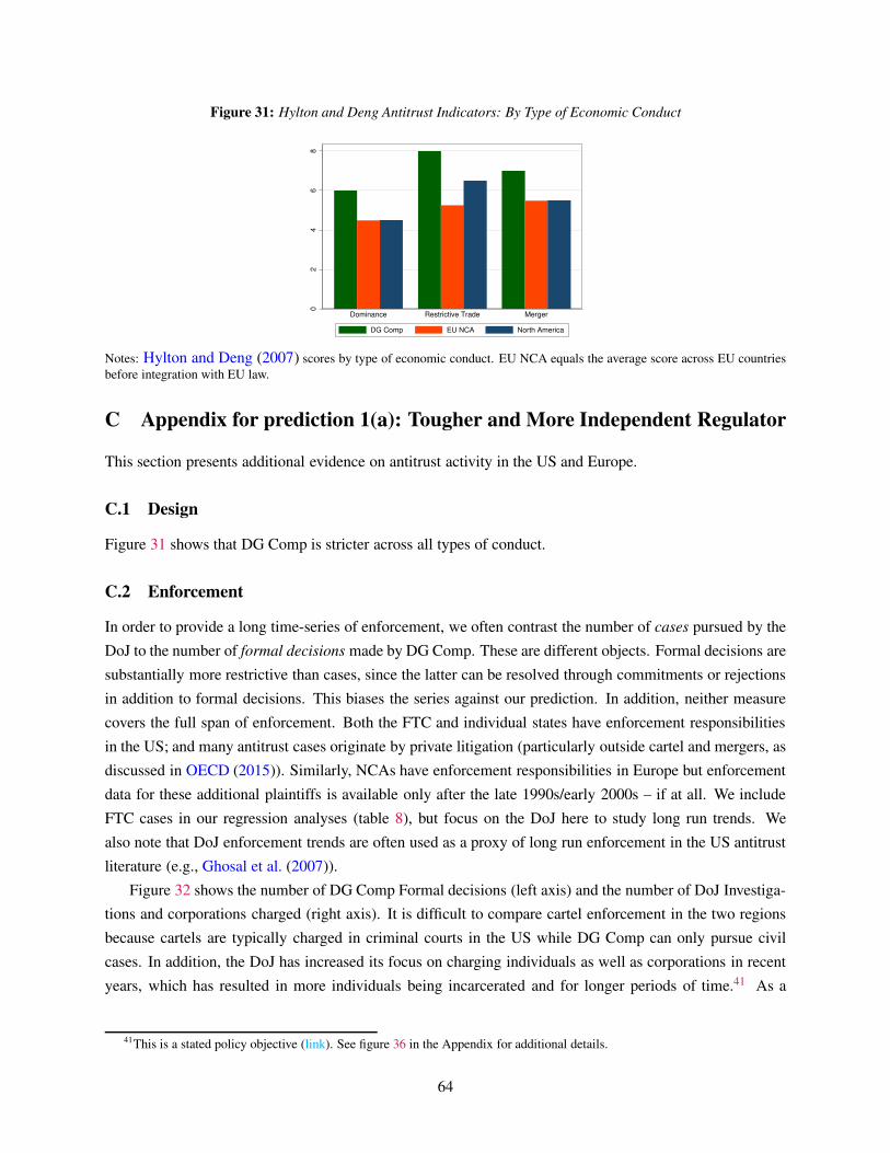
Figure 31: Hylton and Deng Antitrust Indicators: By Type of Economic Conduct

02

46

8Dominance Restrictive Trade Merger

DG Comp EU NCA North America

Notes: Hylton and Deng (2007) scores by type of economic conduct. EU NCA equals the average score across EU countries

before integration with EU law.

C Appendix for prediction 1(a): Tougher and More Independent Regulator

This section presents additional evidence on antitrust activity in the US and Europe.

C.1 Design

Figure 31 shows that DG Comp is stricter across all types of conduct.

C.2 Enforcement

In order to provide a long time-series of enforcement, we often contrast the number of cases pursued by the

DoJ to the number of formal decisions made by DG Comp. These are different objects. Formal decisions are

substantially more restrictive than cases, since the latter can be resolved through commitments or rejections

in addition to formal decisions. This biases the series against our prediction. In addition, neither measure

covers the full span of enforcement. Both the FTC and individual states have enforcement responsibilities

in the US; and many antitrust cases originate by private litigation (particularly outside cartel and mergers, as

discussed in OECD (2015)). Similarly, NCAs have enforcement responsibilities in Europe but enforcement

data for these additional plaintiffs is available only after the late 1990s/early 2000s – if at all. We include

FTC cases in our regression analyses (table 8), but focus on the DoJ here to study long run trends. We

also note that DoJ enforcement trends are often used as a proxy of long run enforcement in the US antitrust

literature (e.g., Ghosal et al. (2007)).

Figure 32 shows the number of DG Comp Formal decisions (left axis) and the number of DoJ Investiga-

tions and corporations charged (right axis). It is difficult to compare cartel enforcement in the two regions

because cartels are typically charged in criminal courts in the US while DG Comp can only pursue civil

cases. In addition, the DoJ has increased its focus on charging individuals as well as corporations in recent

years, which has resulted in more individuals being incarcerated and for longer periods of time.41 As a

41This is a stated policy objective (link). See figure 36 in the Appendix for additional details.

64

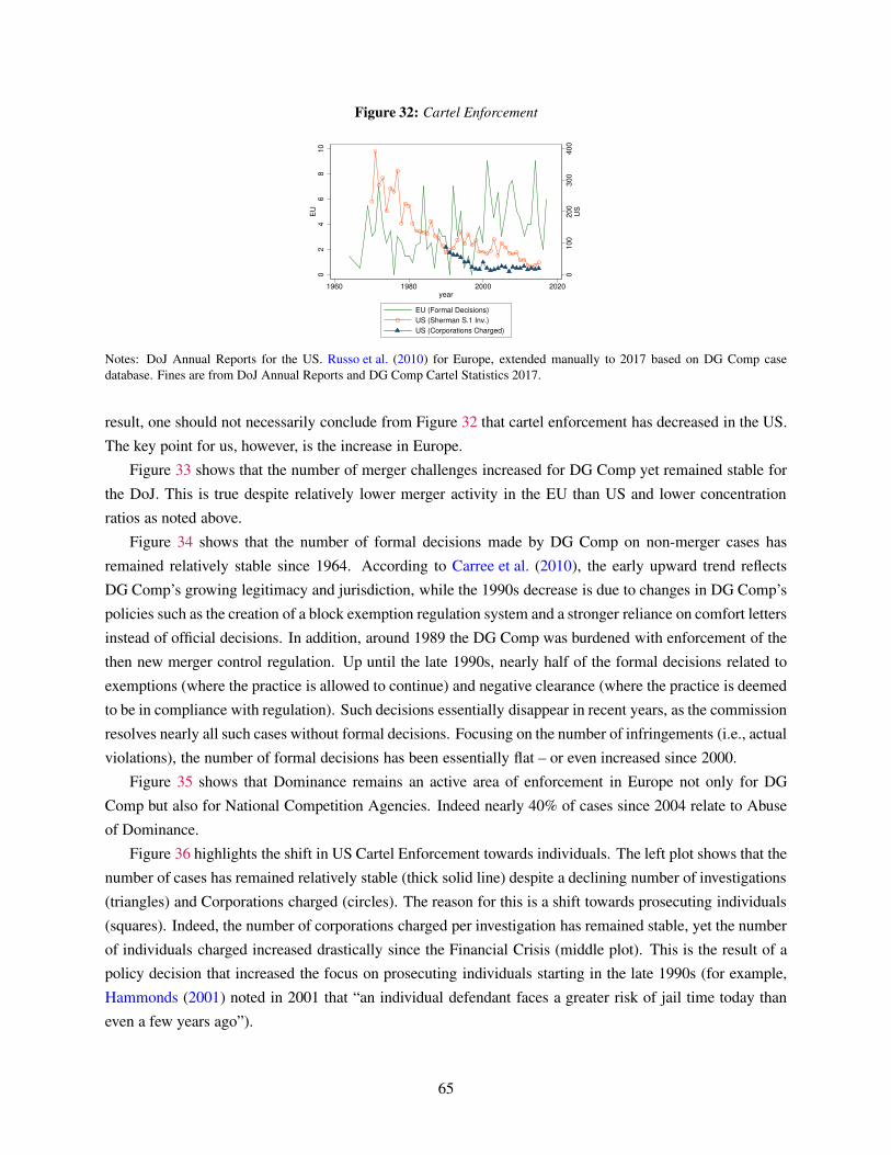
Figure 32: Cartel Enforcement

01

00

20

03

00

40

0U

S

02

46

81

0E

U

1960 1980 2000 2020year

EU (Formal Decisions)

US (Sherman S.1 Inv.)

US (Corporations Charged)

Notes: DoJ Annual Reports for the US. Russo et al. (2010) for Europe, extended manually to 2017 based on DG Comp case

database. Fines are from DoJ Annual Reports and DG Comp Cartel Statistics 2017.

result, one should not necessarily conclude from Figure 32 that cartel enforcement has decreased in the US.

The key point for us, however, is the increase in Europe.

Figure 33 shows that the number of merger challenges increased for DG Comp yet remained stable for

the DoJ. This is true despite relatively lower merger activity in the EU than US and lower concentration

ratios as noted above.

Figure 34 shows that the number of formal decisions made by DG Comp on non-merger cases has

remained relatively stable since 1964. According to Carree et al. (2010), the early upward trend reflects

DG Comp’s growing legitimacy and jurisdiction, while the 1990s decrease is due to changes in DG Comp’s

policies such as the creation of a block exemption regulation system and a stronger reliance on comfort letters

instead of official decisions. In addition, around 1989 the DG Comp was burdened with enforcement of the

then new merger control regulation. Up until the late 1990s, nearly half of the formal decisions related to

exemptions (where the practice is allowed to continue) and negative clearance (where the practice is deemed

to be in compliance with regulation). Such decisions essentially disappear in recent years, as the commission

resolves nearly all such cases without formal decisions. Focusing on the number of infringements (i.e., actual

violations), the number of formal decisions has been essentially flat – or even increased since 2000.

Figure 35 shows that Dominance remains an active area of enforcement in Europe not only for DG

Comp but also for National Competition Agencies. Indeed nearly 40% of cases since 2004 relate to Abuse

of Dominance.

Figure 36 highlights the shift in US Cartel Enforcement towards individuals. The left plot shows that the

number of cases has remained relatively stable (thick solid line) despite a declining number of investigations

(triangles) and Corporations charged (circles). The reason for this is a shift towards prosecuting individuals

(squares). Indeed, the number of corporations charged per investigation has remained stable, yet the number

of individuals charged increased drastically since the Financial Crisis (middle plot). This is the result of a

policy decision that increased the focus on prosecuting individuals starting in the late 1990s (for example,

Hammonds (2001) noted in 2001 that “an individual defendant faces a greater risk of jail time today than

even a few years ago”).

65

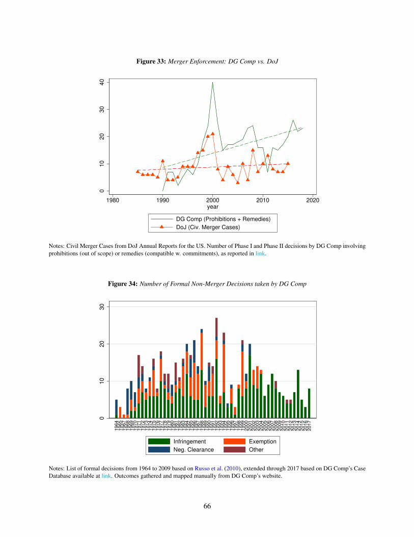
Figure 33: Merger Enforcement: DG Comp vs. DoJ

010

20

30

40

1980 1990 2000 2010 2020year

DG Comp (Prohibitions + Remedies)

DoJ (Civ. Merger Cases)

Notes: Civil Merger Cases from DoJ Annual Reports for the US. Number of Phase I and Phase II decisions by DG Comp involving

prohibitions (out of scope) or remedies (compatible w. commitments), as reported in link.

Figure 34: Number of Formal Non-Merger Decisions taken by DG Comp

010

20

30

19

64

19

65

19

67

19

68

19

69

19

70

19

71

19

72

19

73

19

74

19

75

19

76

19

77

19

78

19

79

19

80

19

81

19

82

19

83

19

84

19

85

19

86

19

87

19

88

19

89

19

90

19

91

19

92

19

93

19

94

19

95

19

96

19

97

19

98

19

99

20

00

20

01

20

02

20

03

20

04

20

05

20

06

20

07

20

08

20

09

20

10

20

11

20

12

20

13

20

14

20

15

20

16

20

17

Infringement Exemption

Neg. Clearance Other

Notes: List of formal decisions from 1964 to 2009 based on Russo et al. (2010), extended through 2017 based on DG Comp’s Case

Database available at link. Outcomes gathered and mapped manually from DG Comp’s website.

66

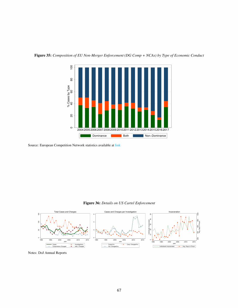
Figure 35: Composition of EU Non-Merger Enforcement (DG Comp + NCAs) by Type of Economic Conduct

020

40

60

80

100

% C

ases b

y T

ype

20042005200620072008200920102011201220132014201520162017

Dominance Both Non−Dominance

Source: European Competition Network statistics available at link

Figure 36: Details on US Cartel Enforcement

05

01

00

15

0

1990 1995 2000 2005 2010 2015year

Cases Investigations

Corporations Charged Indiv. Charged

Total Cases and Charges

02

46

1990 1995 2000 2005 2010 2015year

Cases/Inv Corp. Charged/Inv

Ind. Charged/Inv

Cases and Charges per Investigation

20

04

00

60

08

00

10

00

Avg

. D

ays in

Priso

n

01

02

03

04

05

0In

div

idu

als

In

ca

rce

rate

d

1990 1995 2000 2005 2010 2015year

Individuals Incarcerated Avg. Days in Prison

Incarceration

Notes: DoJ Annual Reports

67

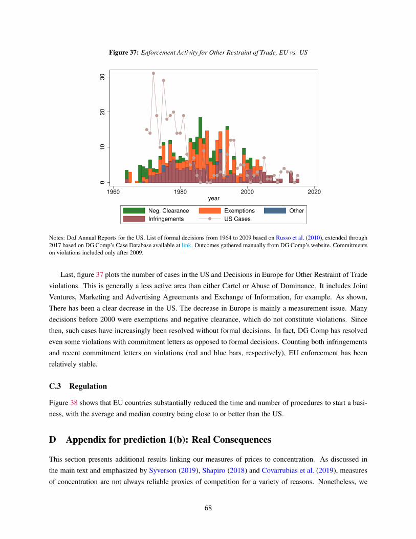
Figure 37: Enforcement Activity for Other Restraint of Trade, EU vs. US

010

20

30

1960 1980 2000 2020year

Neg. Clearance Exemptions Other

Infringements US Cases

Notes: DoJ Annual Reports for the US. List of formal decisions from 1964 to 2009 based on Russo et al. (2010), extended through

2017 based on DG Comp’s Case Database available at link. Outcomes gathered manually from DG Comp’s website. Commitments

on violations included only after 2009.

Last, figure 37 plots the number of cases in the US and Decisions in Europe for Other Restraint of Trade

violations. This is generally a less active area than either Cartel or Abuse of Dominance. It includes Joint

Ventures, Marketing and Advertising Agreements and Exchange of Information, for example. As shown,

There has been a clear decrease in the US. The decrease in Europe is mainly a measurement issue. Many

decisions before 2000 were exemptions and negative clearance, which do not constitute violations. Since

then, such cases have increasingly been resolved without formal decisions. In fact, DG Comp has resolved

even some violations with commitment letters as opposed to formal decisions. Counting both infringements

and recent commitment letters on violations (red and blue bars, respectively), EU enforcement has been

relatively stable.

C.3 Regulation

Figure 38 shows that EU countries substantially reduced the time and number of procedures to start a busi-

ness, with the average and median country being close to or better than the US.

D Appendix for prediction 1(b): Real Consequences

This section presents additional results linking our measures of prices to concentration. As discussed in

the main text and emphasized by Syverson (2019), Shapiro (2018) and Covarrubias et al. (2019), measures

of concentration are not always reliable proxies of competition for a variety of reasons. Nonetheless, we

68

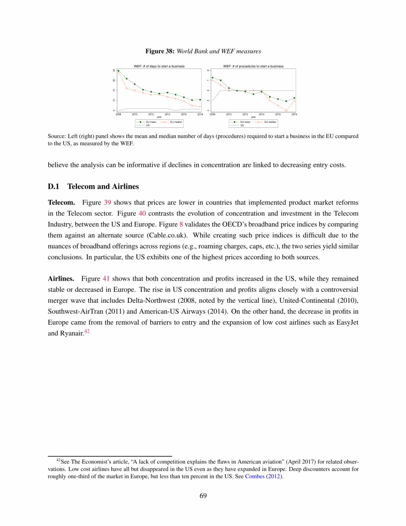
Figure 38: World Bank and WEF measures

51

01

52

02

52008 2010 2012 2014 2016 2018

year

EU mean EU median

US

WEF: # of days to start a business

45

67

8

2008 2010 2012 2014 2016 2018year

EU mean EU median

US

WEF: # of procedures to start a business

Source: Left (right) panel shows the mean and median number of days (procedures) required to start a business in the EU compared

to the US, as measured by the WEF.

believe the analysis can be informative if declines in concentration are linked to decreasing entry costs.

D.1 Telecom and Airlines

Telecom. Figure 39 shows that prices are lower in countries that implemented product market reforms

in the Telecom sector. Figure 40 contrasts the evolution of concentration and investment in the Telecom

Industry, between the US and Europe. Figure 8 validates the OECD’s broadband price indices by comparing

them against an alternate source (Cable.co.uk). While creating such price indices is difficult due to the

nuances of broadband offerings across regions (e.g., roaming charges, caps, etc.), the two series yield similar

conclusions. In particular, the US exhibits one of the highest prices according to both sources.

Airlines. Figure 41 shows that both concentration and profits increased in the US, while they remained

stable or decreased in Europe. The rise in US concentration and profits aligns closely with a controversial

merger wave that includes Delta-Northwest (2008, noted by the vertical line), United-Continental (2010),

Southwest-AirTran (2011) and American-US Airways (2014). On the other hand, the decrease in profits in

Europe came from the removal of barriers to entry and the expansion of low cost airlines such as EasyJet

and Ryanair.42

42See The Economist’s article, “A lack of competition explains the flaws in American aviation” (April 2017) for related obser-

vations. Low cost airlines have all but disappeared in the US even as they have expanded in Europe. Deep discounters account for

roughly one-third of the market in Europe, but less than ten percent in the US. See Combes (2012).

69

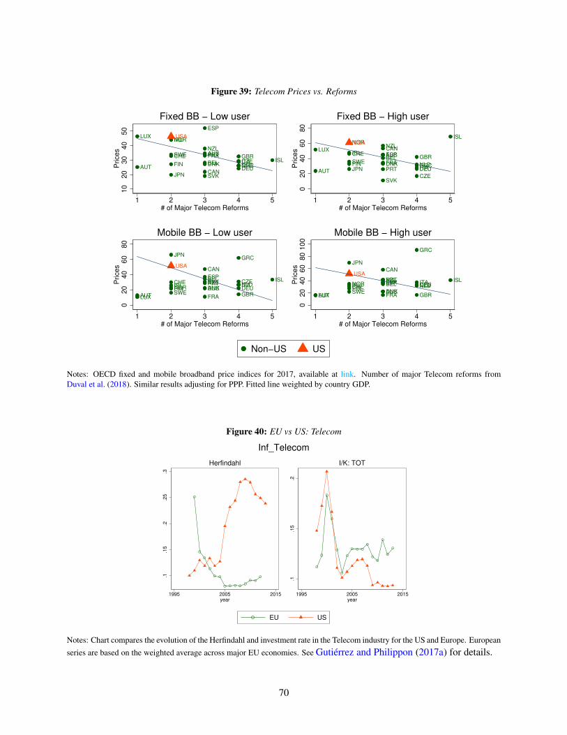
Figure 39: Telecom Prices vs. Reforms

AUS

AUTBEL

CAN

CHECZE

DEUDNK

ESP

FIN

FRA GBR

GRC

IRL

ISLITA

JPN

LUX

NLD

NOR

NZLPRT

SVK

SWE

USA

10

20

30

40

50

Price

s

1 2 3 4 5# of Major Telecom Reforms

Fixed BB − Low user

AUS

AUT

BEL

CANCHE

CZE

DEUDNK

ESP

FIN FRAGBR

GRC

IRL

ISL

ITAJPN

LUX

NLD

NORNZL

PRT

SVK

SWE

USA

02

04

06

08

0P

rice

s

1 2 3 4 5# of Major Telecom Reforms

Fixed BB − High user

AUS

AUT

BEL

CAN

CHE CZEDEUDNK

ESP

FIN

FRA GBR

GRC

IRLISL

ITA

JPN

LUX

NLDNOR

NZLPRTSVK

SWE

USA

02

04

06

08

0P

rice

s

1 2 3 4 5# of Major Telecom Reforms

Mobile BB − Low user

AUSAUT

BEL

CAN

CHE CZEDEU

DNK

ESPFIN

FRA GBR

GRC

IRLISLITA

JPN

LUX

NLDNORNZLPRTSVK

SWE

USA

02

04

06

08

01

00

Price

s

1 2 3 4 5# of Major Telecom Reforms

Mobile BB − High user

Non−US US

Notes: OECD fixed and mobile broadband price indices for 2017, available at link. Number of major Telecom reforms from

Duval et al. (2018). Similar results adjusting for PPP. Fitted line weighted by country GDP.

Figure 40: EU vs US: Telecom

.1.1

5.2

.25

.3

1995 2005 2015year

Herfindahl

.1.1

5.2

1995 2005 2015year

I/K: TOT

Inf_Telecom

EU US

Notes: Chart compares the evolution of the Herfindahl and investment rate in the Telecom industry for the US and Europe. European

series are based on the weighted average across major EU economies. See Gutiérrez and Philippon (2017a) for details.

70

Figure 41: Air Transportation Profits and Concentration, EU vs US−

.2−

.10

.1

1995 2000 2005 2010 2015year

US EU

OS/PROD

.06

.08

.1.1

2.1

4

1995 2000 2005 2010 2015year

US EU

HHI

Notes: Chart compares the evolution of net profit rates and concentration in the Transportation - Air industry (ISIC code 51) for the

US and Europe. Profit rates from OECD STAN. Concentration based on Compustat, adjusted for database coverage using OECD

STAN (i.e., sale shares are defined as the ratio of firm sales to the maximum of Compustat sales and gross output from OECD

STAN). EU firms included only if data for the corresponding country are available in STAN.

D.2 Prices and Concentration

Let us now consider all industries. We use prices from KLEMS and ICP and measures of concentration

from Compustat for the US and ORBIS for Europe. KLEMS and ICP have advantages and limitations.

The main advantage of ICP is that it contains the prices of individual products published in benchmark

surveys every three years since 1999. These are conceptually similar to the Telecom prices presented earlier.

Unfortunately, the product accounts do not map one-to-one into ISIC industries (for which we have measures

of concentration). Based on a detailed comparison of broad ICP product categories and ISIC Industry

descriptions, we were able to identify 7 product categories that map into individual industries, as shown in

Table 6.43

Table 6: Mapping of ICP to ISIC segments

ICP Category KLEMS industry Code

Food and non-alcoholic beverages Food products, beverages and tobacco D10T12

Clothing and footwear Textiles, wearing apparel, leather and related products D13T15

Communication Telecommunications D61

Recreation and culture Arts, entertainment and recreation D90T93

Education Education D85

Restaurants and hotels Accommodation and food service activities D55T56

Construction Construction D41T43

By contrast, the main advantage of KLEMS is that it provides complete coverage across industries,

and includes measures of wages and productivity needed to estimate mark-ups. Unlike ICP data, however,

43Compustat and ORBIS provide limited coverage for Education. We confirm that results are robust to excluding this industry.

71

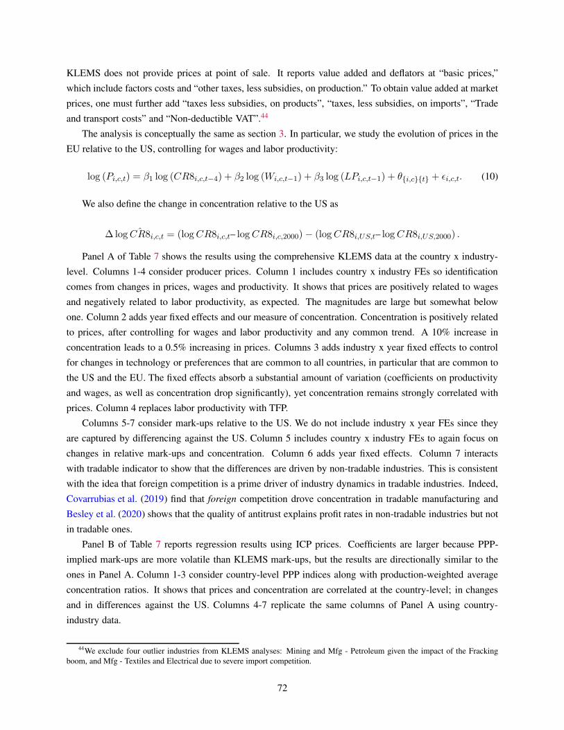
KLEMS does not provide prices at point of sale. It reports value added and deflators at “basic prices,”

which include factors costs and “other taxes, less subsidies, on production.” To obtain value added at market

prices, one must further add “taxes less subsidies, on products”, “taxes, less subsidies, on imports”, “Trade

and transport costs” and “Non-deductible VAT”.44

The analysis is conceptually the same as section 3. In particular, we study the evolution of prices in the

EU relative to the US, controlling for wages and labor productivity:

log (Pi,c,t) = β1 log (CR8i,c,t−4) + β2 log (Wi,c,t−1) + β3 log (LPi,c,t−1) + θ{i,c}{t} + ǫi,c,t. (10)

We also define the change in concentration relative to the US as

∆ log ˆCR8i,c,t = (logCR8i,c,t– logCR8i,c,2000)− (logCR8i,US,t– logCR8i,US,2000) .

Panel A of Table 7 shows the results using the comprehensive KLEMS data at the country x industry-

level. Columns 1-4 consider producer prices. Column 1 includes country x industry FEs so identification

comes from changes in prices, wages and productivity. It shows that prices are positively related to wages

and negatively related to labor productivity, as expected. The magnitudes are large but somewhat below

one. Column 2 adds year fixed effects and our measure of concentration. Concentration is positively related

to prices, after controlling for wages and labor productivity and any common trend. A 10% increase in

concentration leads to a 0.5% increasing in prices. Columns 3 adds industry x year fixed effects to control

for changes in technology or preferences that are common to all countries, in particular that are common to

the US and the EU. The fixed effects absorb a substantial amount of variation (coefficients on productivity

and wages, as well as concentration drop significantly), yet concentration remains strongly correlated with

prices. Column 4 replaces labor productivity with TFP.

Columns 5-7 consider mark-ups relative to the US. We do not include industry x year FEs since they

are captured by differencing against the US. Column 5 includes country x industry FEs to again focus on

changes in relative mark-ups and concentration. Column 6 adds year fixed effects. Column 7 interacts

with tradable indicator to show that the differences are driven by non-tradable industries. This is consistent

with the idea that foreign competition is a prime driver of industry dynamics in tradable industries. Indeed,

Covarrubias et al. (2019) find that foreign competition drove concentration in tradable manufacturing and

Besley et al. (2020) shows that the quality of antitrust explains profit rates in non-tradable industries but not

in tradable ones.

Panel B of Table 7 reports regression results using ICP prices. Coefficients are larger because PPP-

implied mark-ups are more volatile than KLEMS mark-ups, but the results are directionally similar to the

ones in Panel A. Column 1-3 consider country-level PPP indices along with production-weighted average

concentration ratios. It shows that prices and concentration are correlated at the country-level; in changes

and in differences against the US. Columns 4-7 replicate the same columns of Panel A using country-

industry data.

44We exclude four outlier industries from KLEMS analyses: Mining and Mfg - Petroleum given the impact of the Fracking

boom, and Mfg - Textiles and Electrical due to severe import competition.

72

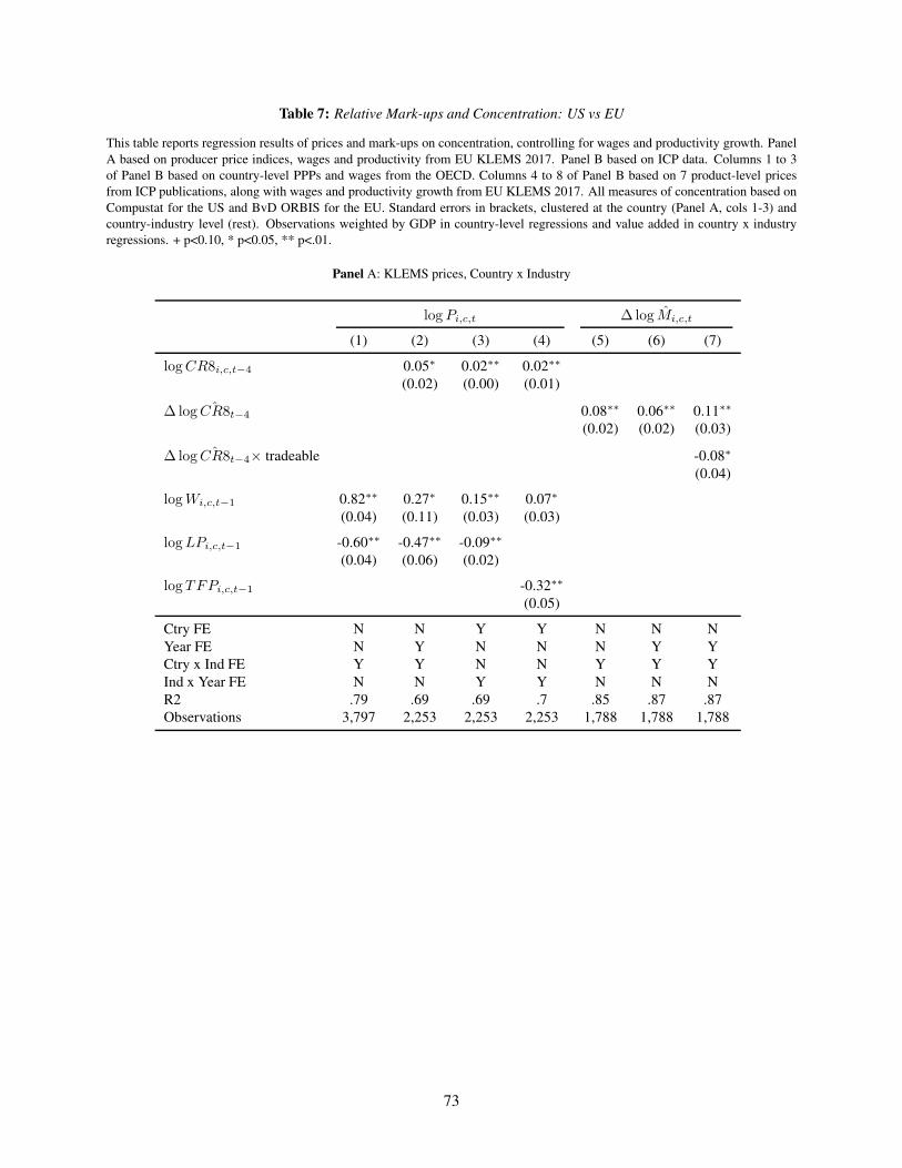
Table 7: Relative Mark-ups and Concentration: US vs EU

This table reports regression results of prices and mark-ups on concentration, controlling for wages and productivity growth. Panel

A based on producer price indices, wages and productivity from EU KLEMS 2017. Panel B based on ICP data. Columns 1 to 3

of Panel B based on country-level PPPs and wages from the OECD. Columns 4 to 8 of Panel B based on 7 product-level prices

from ICP publications, along with wages and productivity growth from EU KLEMS 2017. All measures of concentration based on

Compustat for the US and BvD ORBIS for the EU. Standard errors in brackets, clustered at the country (Panel A, cols 1-3) and

country-industry level (rest). Observations weighted by GDP in country-level regressions and value added in country x industry

regressions. + p<0.10, * p<0.05, ** p<.01.

Panel A: KLEMS prices, Country x Industry

logPi,c,t ∆ log Mi,c,t

(1) (2) (3) (4) (5) (6) (7)

logCR8i,c,t−4 0.05∗ 0.02∗∗ 0.02∗∗

(0.02) (0.00) (0.01)

∆ log ˆCR8t−4 0.08∗∗ 0.06∗∗ 0.11∗∗

(0.02) (0.02) (0.03)

∆ log ˆCR8t−4× tradeable -0.08∗

(0.04)

logWi,c,t−1 0.82∗∗ 0.27∗ 0.15∗∗ 0.07∗

(0.04) (0.11) (0.03) (0.03)

logLPi,c,t−1 -0.60∗∗ -0.47∗∗ -0.09∗∗

(0.04) (0.06) (0.02)

logTFPi,c,t−1 -0.32∗∗

(0.05)

Ctry FE N N Y Y N N N

Year FE N Y N N N Y Y

Ctry x Ind FE Y Y N N Y Y Y

Ind x Year FE N N Y Y N N N

R2 .79 .69 .69 .7 .85 .87 .87

Observations 3,797 2,253 2,253 2,253 1,788 1,788 1,788

73

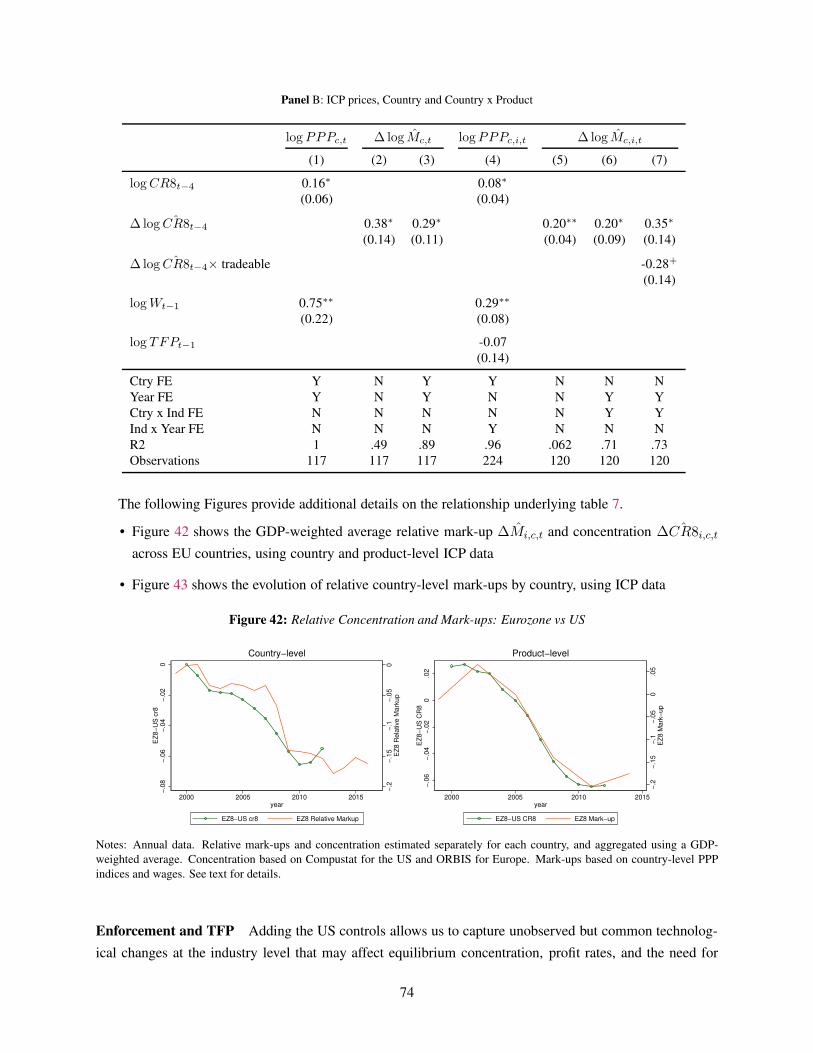
Panel B: ICP prices, Country and Country x Product

logPPPc,t ∆ log Mc,t logPPPc,i,t ∆ log Mc,i,t

(1) (2) (3) (4) (5) (6) (7)

logCR8t−4 0.16∗ 0.08∗

(0.06) (0.04)

∆ log ˆCR8t−4 0.38∗ 0.29∗ 0.20∗∗ 0.20∗ 0.35∗

(0.14) (0.11) (0.04) (0.09) (0.14)

∆ log ˆCR8t−4× tradeable -0.28+

(0.14)

logWt−1 0.75∗∗ 0.29∗∗

(0.22) (0.08)

log TFPt−1 -0.07

(0.14)

Ctry FE Y N Y Y N N N

Year FE Y N Y N N Y Y

Ctry x Ind FE N N N N N Y Y

Ind x Year FE N N N Y N N N

R2 1 .49 .89 .96 .062 .71 .73

Observations 117 117 117 224 120 120 120

The following Figures provide additional details on the relationship underlying table 7.

• Figure 42 shows the GDP-weighted average relative mark-up ∆Mi,c,t and concentration ∆ ˆCR8i,c,t

across EU countries, using country and product-level ICP data

• Figure 43 shows the evolution of relative country-level mark-ups by country, using ICP data

Figure 42: Relative Concentration and Mark-ups: Eurozone vs US

−.2

−.1

5−

.1−

.05

0E

Z8

Re

lative

Ma

rku

p

−.0

8−

.06

−.0

4−

.02

0E

Z8

−U

S c

r8

2000 2005 2010 2015year

EZ8−US cr8 EZ8 Relative Markup

Country−level−

.2−

.15

−.1

−.0

50

.05

EZ

8 M

ark

−u

p

−.0

6−

.04

−.0

20

.02

EZ

8−

US

CR

8

2000 2005 2010 2015year

EZ8−US CR8 EZ8 Mark−up

Product−level

Notes: Annual data. Relative mark-ups and concentration estimated separately for each country, and aggregated using a GDP-

weighted average. Concentration based on Compustat for the US and ORBIS for Europe. Mark-ups based on country-level PPP

indices and wages. See text for details.

Enforcement and TFP Adding the US controls allows us to capture unobserved but common technolog-

ical changes at the industry level that may affect equilibrium concentration, profit rates, and the need for

74

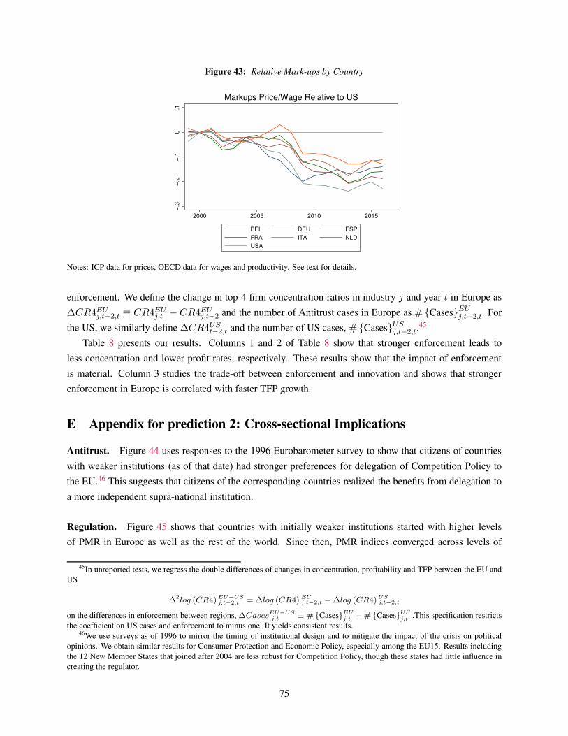
Figure 43: Relative Mark-ups by Country

−.3

−.2

−.1

0.1

2000 2005 2010 2015

BEL DEU ESP

FRA ITA NLD

USA

Markups Price/Wage Relative to US

Notes: ICP data for prices, OECD data for wages and productivity. See text for details.

enforcement. We define the change in top-4 firm concentration ratios in industry j and year t in Europe as

∆CR4EUj,t−2,t ≡ CR4EU

j,t − CR4EUj,t−2 and the number of Antitrust cases in Europe as # {Cases}EU

j,t−2,t. For

the US, we similarly define ∆CR4USt−2,t and the number of US cases, # {Cases}US

j,t−2,t.45

Table 8 presents our results. Columns 1 and 2 of Table 8 show that stronger enforcement leads to

less concentration and lower profit rates, respectively. These results show that the impact of enforcement

is material. Column 3 studies the trade-off between enforcement and innovation and shows that stronger

enforcement in Europe is correlated with faster TFP growth.

E Appendix for prediction 2: Cross-sectional Implications

Antitrust. Figure 44 uses responses to the 1996 Eurobarometer survey to show that citizens of countries

with weaker institutions (as of that date) had stronger preferences for delegation of Competition Policy to

the EU.46 This suggests that citizens of the corresponding countries realized the benefits from delegation to

a more independent supra-national institution.

Regulation. Figure 45 shows that countries with initially weaker institutions started with higher levels

of PMR in Europe as well as the rest of the world. Since then, PMR indices converged across levels of

45In unreported tests, we regress the double differences of changes in concentration, profitability and TFP between the EU and

US

∆2log (CR4)EU−US

j,t−2,t = ∆log (CR4)EUj,t−2,t −∆log (CR4) US

j,t−2,t

on the differences in enforcement between regions, ∆CasesEU−US,j,t ≡ # {Cases}EU

j,t −# {Cases}US

j,t .This specification restricts

the coefficient on US cases and enforcement to minus one. It yields consistent results.46We use surveys as of 1996 to mirror the timing of institutional design and to mitigate the impact of the crisis on political

opinions. We obtain similar results for Consumer Protection and Economic Policy, especially among the EU15. Results including

the 12 New Member States that joined after 2004 are less robust for Competition Policy, though these states had little influence in

creating the regulator.

75

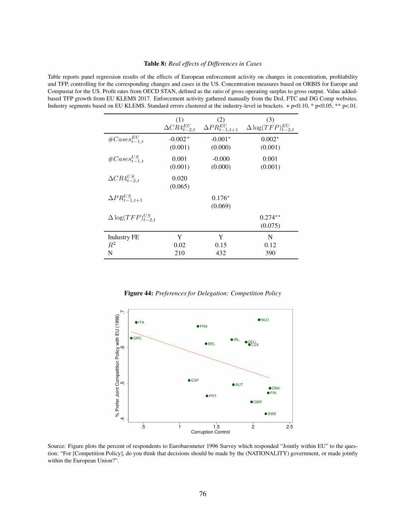
Table 8: Real effects of Differences in Cases

Table reports panel regression results of the effects of European enforcement activity on changes in concentration, profitability

and TFP, controlling for the corresponding changes and cases in the US. Concentration measures based on ORBIS for Europe and

Compustat for the US. Profit rates from OECD STAN, defined as the ratio of gross operating surplus to gross output. Value added-

based TFP growth from EU KLEMS 2017. Enforcement activity gathered manually from the DoJ, FTC and DG Comp websites.

Industry segments based on EU KLEMS. Standard errors clustered at the industry-level in brackets. + p<0.10, * p<0.05, ** p<.01.

(1) (2) (3)

∆CR4EUt−2,t ∆PREU

t−1,t+1 ∆ log(TFP )EUt−2,t

#CasesEUt−1,t -0.002+ -0.001∗ 0.002∗

(0.001) (0.000) (0.001)

#CasesUSt−1,t 0.001 -0.000 0.001

(0.001) (0.000) (0.001)

∆CR4USt−2,t 0.020

(0.065)

∆PRUSt−1,t+1 0.176∗

(0.069)

∆ log(TFP )USt−2,t 0.274∗∗

(0.075)

Industry FE Y Y N

R2 0.02 0.15 0.12

N 210 432 390

Figure 44: Preferences for Delegation: Competition Policy

AUT

BEL DEU

DNK

ESP

FIN

FRA

GBR

GRC IRL

ITA

LUX

NLD

PRT

SWE

.4.5

.6.7

% P

refe

r Join

t C

om

petition P

olic

y w

ith E

U (

1996)

.5 1 1.5 2 2.5Corruption Control

Source: Figure plots the percent of respondents to Eurobarometer 1996 Survey which responded “Jointly within EU” to the ques-

tion: “For [Competition Policy], do you think that decisions should be made by the (NATIONALITY) government, or made jointly

within the European Union?”.

76

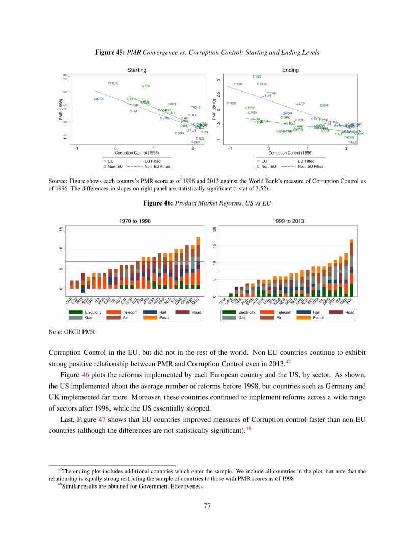
Figure 45: PMR Convergence vs. Corruption Control: Starting and Ending Levels

AUT

BEL

CZE

DEU

DNK

ESP

FIN

FRA

GBR

GRCHUN

IRL

ITA

NLD

POL

PRT

SWE

AUS

CAN

CHE

ISLJPN

KOR

MEX

NOR

NZL

TUR

USA

1.5

22.5

33.5

PM

R (

1998)

−1 0 1 2Corruption Control (1996)

EU EU Fitted

Non−EU Non−EU Fitted

Starting

AUT

BEL

BGRCYP

CZEDEU

DNK

ESP

EST FIN

FRA

GBR

GRC

HRV

HUNIRL

ITA

LTULUX

LVA MLT

NLD

POL

PRT

ROU

SVK

SVN

SWE

AUS

BRA

CANCHECHL

CHNIDN

IND

ISL

ISR

JPN

KORMEX

NOR

NZL

RUS

TUR

USA

ZAF

11.5

22.5

3P

MR

(2013)

−1 0 1 2Corruption Control (1996)

EU EU Fitted

Non−EU Non−EU Fitted

Ending

Source: Figure shows each country’s PMR score as of 1998 and 2013 against the World Bank’s measure of Corruption Control as

of 1996. The differences in slopes on right panel are statistically significant (t-stat of 3.52).

Figure 46: Product Market Reforms, US vs EU

05

10

15

CHELU

XPR

TSVK

GRC

ITAKO

RCZE

IRLAU

TESP

NOR

BELFR

AJP

NUSA

AUSDNKNLD FIN

SWECAN

GBR

DEU

1970 to 1998

Electricity Telecom Rail Road

Gas Air Postal

05

10

15

20

USA

CAN

FINGBR

AUSSW

EAU

TDNKLU

XJP

NKO

RNORDEU

NLD

CHEESP

BELFR

AIR

LGRCPR

TIT

ACZE

SVK

1999 to 2013

Electricity Telecom Rail Road

Gas Air Postal

Note: OECD PMR

Corruption Control in the EU, but did not in the rest of the world. Non-EU countries continue to exhibit

strong positive relationship between PMR and Corruption Control even in 2013.47

Figure 46 plots the reforms implemented by each European country and the US, by sector. As shown,

the US implemented about the average number of reforms before 1998, but countries such as Germany and

UK implemented far more. Moreover, these countries continued to implement reforms across a wide range

of sectors after 1998, while the US essentially stopped.

Last, Figure 47 shows that EU countries improved measures of Corruption control faster than non-EU

countries (although the differences are not statistically significant).48

47The ending plot includes additional countries which enter the sample. We include all countries in the plot, but note that the

relationship is equally strong restricting the sample of countries to those with PMR scores as of 199848Similar results are obtained for Government Effectiveness

77

Figure 47: World Bank and WEF measures

AUT

BELBGR

CYP

CZEDEU

DNK

ESP

EST

FINFRA

GBR

GRC

HRV

HUN

IRL

ITA

LTU

LUX

LVA

MLT

NLD

POL

PRT

ROU

SVK

SVN

SWE

AUS

BRA

CAN

CHE

CHL

CHN

COL

EGY

IDN

IND

ISL

ISR

JPN

KOR

MEX

NOR

NZL

PER

RUS

TUR

UKR

USA

ZAF

−1

−.5

0.5

1C

orr

up

tio

n C

on

tro

l (

20

16

− 1

99

6)

−1 0 1 2Corruption Control (1996)

EU Non−EU

World Bank: Corruption Control

Source: Change in the World Bank’s measure of Corruption Control from 1996 to 2016 against the starting value.

F History of Antitrust and Regulatory Institutions on both Sides of the At-

lantic

F.1 Antitrust Institutions in the US

Antitrust laws are influenced by the evolution of market structure, business practices, and economic analy-

sis. The Sherman Act of 1890 was motivated by the growth of large-scale businesses during the industrial

revolution. The Clayton Act of 1914 was the first attempt to deal with anti-competitive mergers and acqui-

sitions. It was motivated by larger mergers that fell outside the purview of the Sherman Act of 1890. The

Clayton Act prohibited any company from buying the stock of another company when “the effect of such

acquisition may be substantially to lessen competition”.49 In the 1950’s the Clayton Act was expanded to

include assets as well as stock acquisitions.

The economic understanding of antitrust has also evolved significantly over time, in particular follow-

ing the Chicago school revolution, which put economic efficiency at the center of antitrust policy, and the

influential book by Robert Bork (Bork, 1978). As Kwoka and White (2014) explain “the skepticism and

even some hostility toward big business that characterized the initial period of antitrust have been replaced

by current policy that evaluates market structure and business practices differently.” For instance, high con-

centration does not necessarily imply market power. These evolutions are reflected in the various vintages

of the Merger Guidelines, initially developed by the DoJ’s Antitrust Division in 1968. Major revisions to

the guidelines took place in 1982 and 2010.

At the federal level, the relevant responsibilities are mostly divided between the DoJ Antitrust Division

and the Federal Trade Commission (FTC), although some industries, such as railways and Telecoms, also

have their own regulators. The FTC is a quasi-judicial, independent regulatory agency led by five commis-

sioners. Each commissioner is nominated by the President, confirmed by the Senate, and serves a seven-year

term. The terms are staggered and no more than three commissioners can be from the same political party.

The President designates one of the commissioners as the Chairman. The DoJ is part of the executive branch,

49This is from Section 7 of the Clayton Act. A distinctive feature of Section 7 is that it lowered the standard of proof for the

anti-competitive effects. Under Section 7, mergers could be forbidden when “the trend to a lessening of competition in a line

of commerce was still in its incipiency,” whereas the Sherman Act requires proof of extant harm to competition, as explained in

Institute (2013). The original Section 7, enacted in 1914, only prohibited the acquisitions of “stock” of one corporation by another

corporation, and, by its explicit term, it was not applied to the “assets” acquisitions. As a result, businesses found their ways to

evade the prohibition by buying target corporation’s assets. Congress amended Section 7 to fix this loophole.

78

operating under the US Attorney General. An Assistant Attorney General, nominated by the President and

confirmed by the Senate, leads the Antitrust Division. The authorities of the FTC and DoJ can overlap, but

in practice they tend focus on particular industries or markets. For example, the DoJ typically investigates

mergers in the Financial Services, Telecommunications, and Agricultural Industries, while the FTC typically

investigates mergers in the Defense, Pharmaceutical, and Retail Industries. Before opening an investigation,

the agencies consult with one another. State Attorney Generals (AGs) and private courts also play a role

in antitrust enforcement. State AGs can bring actions to enforce their state’s own antitrust laws, either as

federal antitrust suits on behalf of individuals residing within their states, or on behalf of the state as a pur-

chaser. Similarly, private plaintiffs may bring civil actions for violations of the federal antitrust laws, with

the exception of cartel and mergers (see OECD (2015) for additional details on the interplay between public

and private enforcement).

F.2 Antitrust Institutions in Europe

The history of EU antitrust is more recent. In 1957 the Treaty of Rome laid the foundations of European

competition policies, building on the Treaty of Paris that established the European Coal and Steel Commu-

nity (ECSC) in 1951. Article 3(1)(g) of the Treaty of Rome envisions “a system ensuring that competition

in the internal market is not distorted”. Council Regulation 17 made the enforcement powers effective in

1962, and the EU Commission made its first decision in 1964. This regulation was modernized by regula-

tion 1/2003, which has been effective since May 2004. Articles 101 (ex. 81) of the Treaty of Rome deals

with horizontal conduct, vertical restraint, licensing, and joint ventures. Article 102 (ex. 82) deals with

the anti-competitive effects of dominant position. Merger regulations were added in 1989. Member states

have national competition authorities (NCAs) to deal with cases that have national impact. The European

Commissioner for Competition and the Directorate-General for Competition (DG Comp) enforce European

competition law in cooperation with the NCAs. DG Comp prepares decisions in three broad areas: antitrust,

mergers, and state aid.

An interesting debate – and important for our analysis – concerns the influence of the US on Europe.

This debate has evolved in three stages. At first, the common wisdom was that EU laws were direct descen-

dants of US laws. Berger (1998) challenged this view and showed that EU laws also had their own “indige-

nous” traditions. Since then, scholars have reached a more balanced view. For instance, Leucht and Marquis

(2013) study the exchange of ideas between the US and Europe and Leucht (2009) explores how the tradi-

tionally protectionist economies of Western Europe agreed on common competition rules. Nonetheless, the

overall theme is that ideas and institutions have largely converged across regions.

Some changes in recent years have been more qualitative but nonetheless important. In particular, the

2004 changes made the DG Comp more transparent and more accountable to the public. It also clarified the

notion of unilateral effects in a way that resembles the US approach. Foncel et al. (2007) focus on important

changes in the new EC Merger Regulation of 2004. At the same time, the role of economists within the DG

comp has increased during the 2000’s, in particular with the creation of the position of Chief Competition

Economist in 2003. The position of EU commissioner for competition is prestigious, attracts high caliber

politicians, and benefits from strong public recognition.

79

F.3 Regulatory Institutions in the US

The US began a long process of economic deregulation in the 1970s which, over the next three decades,

would cover the Air (1978), Road (1980) and Rail (1981) transportation industries, Electric Power (1978+),

Natural Gas (1978), Banking (1980) and Telecommunications (1996) (OECD, 1999). The process of dereg-

ulation was deemed a success, with estimates of price reductions ranging from 30-75% across sectors, in

addition to improved product quality and choice (OECD, 1999). In 1999, the OECD noted that the “United

States has been a world leader in regulatory reform for a quarter century. Its reforms and their results

helped launch a global reform movement that has brought benefits to many millions of people”.

The deregulation process was led by the Federal Government, though State and Local governments also

have regulatory responsibilities. At the federal level, new laws are written only by congress; but more than

60 executive agencies are authorized to issue subordinate regulations. Indeed, these executive agencies

issue thousands of new regulations each year. Federal Regulations are compiled in The Code of Federal

Regulations (CFR).

Importantly, economic deregulation did not coincide with a reduction of total regulation. Environmental,

health, and safety regulations increased substantially over the same period – and have continued to increase.

As of 2017, the CFR spans nearly 180,000 pages following an eight-fold expansion over the past 56 years

(Davis, 2017). The substantial rise in the scale and complexity of Federal Regulation has led some authors

to argue that excessively complex regulations are increasing barriers to entry.

State and Local government regulation further add to the regulatory burden. It is harder to summarize

the scale or growth of such regulation, but the increase has also been significant. Occupational Licensing

is an area that has received substantial attention. CEA (2016), for example, show that the share of workers

required to obtain a license increased from under 5 percent in the 1950s to over 25 percent in 2008 – in large

part because of greater prevalence of licensing requirements at the State-level.

F.4 Regulatory Institutions in Europe

As with Antitrust, regulatory reform efforts in the EU are more recent. Some countries (such as the UK)

pursued economic deregulation independently as early as 1979. But concerted, EU-wide reform efforts

started (on a limited scope) in 1985 with the Single Market Plan, and accelerated in the 2000s with the

introduction of the Lisbon Strategy.50 With regards to product market competition, the Lisbon Strategy

aimed “at opening up product markets to competition in particular by completing the internal market for

goods and services, by removing obstacles to competition in Member States and by creating a business

environment more conducive to market entry and exit.” (Zeitz, 2009) While the Lisbon Strategy failed in

other dimensions, substantial product market reforms were implemented. And today, it is hard to under-state

the increase of competitiveness arising from a single market – and for many countries, a single currency

(Gilchrist et al., 2017). Indeed, European economies have some of the lowest barriers to trade and foreign

investment in the world.

50The Lisbon Strategy aimed to make the EU “the most competitive and dynamic knowledge-based economy in the world

capable of sustainable economic growth with more and better jobs and greater social cohesion” by 2010 (link).

80

Importantly, EU institutions have only partial oversight over Member State’s regulatory environments.

The EU can either directly prohibit certain domestic regulations (e.g., prohibition of Golden Shares and

price controls in transportation industries), can work with member countries to achieve mutual recognition

of restrictions, or can enact case law based on a treaty (e.g., ongoing regulation of State Aid by DG Comp).

But beyond that, member states must implement reforms directly. This does not mean, however, that the EU

has no influence over reform efforts.

Take the implementation of the Lisbon Strategy, for example. The overall objectives were set jointly

by the EU and Member States. From then on, Member States were in charge of implementation, but were

also required to submit reports to the European Commission on an on-going basis: the so-called Cardiff

Reports from 200-2004, followed by National Reform Programs and implementation reports. The EU used

those reports to continuously monitor and disclose progress – including the creation of the Microeconomic

Reform database (MICREF) which compiled and tracked progress across all states. Indeed, EU and peer

pressure were seen as key ‘embarrassment tools’ available to encourage reform. And, if countries still

fail to implement required reforms, the Commission may curtail the allocation of the EU Cohesion Funds.

Last, for states in the process of accession, stringent reform requirements are negotiated in advance – as

evidenced by the substantial reforms implemented at new EU Member States in Central and Eastern Europe

(Jens and Johannes, 2004).

G Data

The data sources used throughout the paper are summarized in Table 9. Items in italics are included in the

main analysis dataset used in regression analyses. These include industry-level macro data from OECD

STAN and EU KLEMS 2017; concentration measures constructed from Compustat (US and EU) and BvD

ORBIS (EU); and a compilation of antitrust cases detailing the relevant industry and type of economic

conduct by case. We describe the data gathering and mapping exercise for these datasets in the remainder

of this section. The data sources in upright text are used to generate the remaining Tables and Figures in the

text. The associated data sources and manipulations are fully described in the text.

G.1 EU KLEMS

We start with the September 2017 release of EU KLEMS, available at link. This release covers data for 29

countries – the EU-28 plus the United States. We focus on the output datasets, particularly the value added

and value added-implied TFP series.

Data is sourced across all countries as reported, and aggregated to the segments of Dottling et al. (2017)

in order to use the corresponding ORBIS concentration series. To be specific, KLEMS data is available at

the sector level (19 groups) following the ISIC Rev. 4 hierarchy. Data for some sectors is further broken out

(e.g., manufacturing is split into 11 industries), resulting in 34 categories. However, data is not always for the

most granular segments (e.g., capital data for segments D45, D46 and D47 is missing for several countries),

We consider the most granular segments for which data is available, which includes 31 categories. We

then exclude Real Estate (L), Public Administration (O), Households as employers (T) and activities of

81

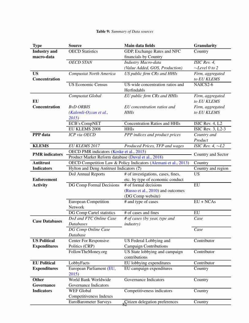
Table 9: Summary of Data sources

Type Source Main data fields Granularity

Industry and

macro-data

OECD Statistics GDP, Exchange Rates and NFC

financials by Country

Country

OECD STAN Industry Macro-data

(Value Added, GOS, Production)

ISIC Rev. 4,

∼Level 0 to 2

US

Concentration

Compustat North America US public firm CRs and HHIs Firm, aggregated

to EU KLEMS

US Economic Census US-wide concentration ratios and

Herfindahls

NAICS2-6

EU

Concentration

Compustat Global EU public firm CRs and HHIs Firm, aggregated

to EU KLEMS

BvD ORBIS

(Kalemli-Ozcan et al.,

2015)

EU concentration ratios and

HHIs

Firm, aggregated

to EU KLEMS

ECB’s CompNET Concentration Ratios and HHIs ISIC Rev. 4, L2

EU KLEMS 2008 HHIs ISIC Rev. 3, L2-3

PPP data ICP via OECD PPP indices and product prices Country and

Product

KLEMS EU KLEMS 2017 Produced Prices, TFP and wages ISIC Rev. 4, ∼L2

PMR indicatorsOECD PMR indicators (Koske et al., 2015)

Country and SectorProduct Market Reform database (Duval et al., 2018)

Antitrust

Indicators

OECD Competition Law & Policy Indicators (Alemani et al., 2013) Country

Hylton and Deng Antitrust Indicators (?) Country and region

Enforcement

Activity

DoJ Annual Reports # of investigations, cases, fines,

etc. by type of economic conduct

US

DG Comp Formal Decisions # of formal decisions

(Russo et al., 2010) and outcomes

(DG Comp website)

EU

European Competition

Network

# and type of cases EU + NCAs

DG Comp Cartel statistics # of cases and fines EU

Case DatabasesDoJ and FTC Online Case

Databases

# of cases (by year, type and

industry)

Case

DG Comp Online Case

Database

Case

US Political

Expenditures

Center For Responsive

Politics (CRP)

US Federal Lobbying and

Campaign Contributions

Contributor

FollowTheMoney.org US State lobbying and campaign

contributions

Contributor

EU Political

Expenditures

LobbyFacts EU lobbying expenditures Contributor

European Parliament (EU,

2015)

EU campaign expenditures Country

Other

Governance

Indicators

World Bank Worldwide

Governance Indicators

Governance Indicators Country

WEF Global

Competitiveness Indexes

Competitiveness indicators Country

EuroBarometer Surveys Citizen delegation preferences Country82

extra-territorial bodies (U); leaving 27 industry groupings, as summarized in Table 10. Segments listed

as ‘excluded’ are excluded from our analyses. Those with a ‘0’ are captured by other (typically more

granular) categories. All other datasets are mapped to these 27 industry groupings. All nominal quantities

are converted to dollars using the OECD’s exchange rates, available at link.

G.2 OECD STAN

Our second main source is OECD STAN. We use data from OECD Table STANI4_2016, which follows

ISIC Rev. 4 segments. These data are available for 36 countries including the EU-28, the US as well as

several other advanced economies (including Australia, Japan, Korea, Canada, Switzerland and Chile). That

said, we restrict the sample to the EU plus US in our regression analyses. Both KLEMS and STAN are

defined based on ISIC Rev. 4, yet STAN provides more granularity than KLEMS. As a result, we can map

STAN to our chosen KLEMS segments directly.

STAN includes measures of production, intermediate inputs, value added, labor costs, (gross and net)

operating surplus, employment, and capital. Our main analysis fields include:

• Value added (VALU)

• Production (gross output) at current prices (PROD)

• Gross operating surplus and mixed income (GOS)

• Net operating surplus and mixed income (NOS)

We convert all nominal quantities to US dollars using the OECD’s exchange rates, available at link. And

then define the profit rate as the ratio of GOS to PROD.51 We aggregate across EU countries by taking the

weighted average (by the corresponding denominator in each ratio).

G.3 Compustat

We use Compustat North America and Compustat Global to compute US and EU-wide concentration ratios.

Compustat includes all public (and some private) firms in the US and EU. US (EU) data are available from

1950 (1987), but coverage is fairly thin until the 1970s (late-1990s). In particular, we download tables Funda,

Company and exrt_mth from both datasets. We use the reported exchange rates to convert all financials to

USD. We apply standard screens (consol = “C”, indfmt = “INDL”, datafmt = “STD”, popsrc = “D” for the

US) and exclude firm-year observations with missing year, sales, assets, or gvkey.52 We focus on the 1990

period for the US and post-2000 period for the EU, and assign firms to countries using headquarter location

(LOC). We use a shorter period for the EU because several stock markets are added beforehand, resulting in

drastic changes in coverage. The sample stabilizes by the early 2000’s.

We use the industry codes in the Compustat Company table. NAICS codes are missing for few firms, so

we map those firms to the most common NAICS-4 industry among those firms with the same SIC code and

51Most of our results are robust to using net profit rates (OS/PROD or OS/VA). However, depreciation series are often available

over shorter periods and can be quite volatile in some segments (see Dottling et al. (2017)) so we focus on Gross Operating Surplus.52We also address selected data issues manually (e.g., outliers in sales growth, especially when reported currency changes)

83

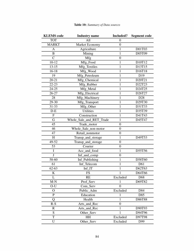
Table 10: Summary of Data sources

KLEMS code Industry name Included? Segment code

TOT All 0

MARKT Market Economy 0

A Agriculture 1 D01T03

B Mining 1 D05T09

C Mfg 0

10-12 Mfg_Food 1 D10T12

13-15 Mfg_Textiles 1 D13T15

16-18 Mfg_Wood 1 D16T18

19 Mfg_Petroleum 1 D19

20-21 Mfg_Chemical 1 D20T21

22-23 Mfg_Rubber 1 D22T23

24-25 Mfg_Metal 1 D24T25

26-27 Mfg_Electrical 1 D26T27

28 Mfg_Machinery 1 D28

29-30 Mfg_Transport 1 D29T30

31-33 Mfg_Other 1 D31T33

D-E Utilities 1 D35T39

F Construction 1 D41T43

G Whole_Sale_and_RET_Trade 1 D45T47

45 Trade_motor 0

46 Whole_Sale_non-motor 0

47 Retail_nonmotor 0

H Transp_and_storage 1 D49T53

49-52 Transp_and_storage 0

53 Courier 0

I Acc_and_food 1 D55T56

J Inf_and_comp 0

58-60 Inf_Publishing 1 D58T60

61 Inf_Telecom 1 D61

62-63 Inf_IT 1 D62T63

K FS 1 D64T66

L RE Excluded D68

M-N Prof_Serv 1 D69T82

O-U Com_Serv 0

O Public_Adm Excluded D84

P Education 1 D85

Q Health 1 D86T88

R-S Arts_and_Rec 0

R Arts_and_Rec 1 D90T93

S Other_Serv 1 D94T96

T HH Excluded D97T98

U Other_Serv Excluded D99

84

non-missing NAICS. We also map all retired/new NAICS codes from the 1997, 2002 and 2012 versions to

NAICS 2007 using the concordances in link. We then map firms to our desired segments using the NAICS

2007 to ISIC Rev. 4 concordance available at link. In particular, we map each NAICS-6 segment to the

most common ISIC Level 2 segment (by number of mappings) based on the the concordance. This mapping

is one-to-one for most NAICS-6 segments; and for the remaining segments there is usually a single most

common ISIC Level 2 segment. For the few cases where NAICS-6 segments map with equal likelihood to

more than one ISIC Level 2 segment, we follow the same methodology but with NAICS-5 codes (and so

on).53 We then map each ISIC Rev. 4 Level 2 segments to our selected KLEMS industries.

We use the resulting dataset to compute Concentration Ratios. Compustat coverage as a share of the

economy varies over time (as more firms go public) and across industries (depending on the nature of

production). To ensure CRs are stable over time and across industries, we adjust Compustat CRs for database

coverage using total gross output from OECD STAN:

CR4jt =

∑

i∈{j,top4}saleCPSTAT

it

sCPSTATjt

× cMAjt

where sCPSTATit denotes sales for firm i which belongs to industry j and sCPSTAT

jt denotes sales across

all Compustat firms in industry j. cMAjt denotes the coverage adjustment, equal to a three-year centered

moving average of the yearly coverage ratio (cjt =sCPSTATjt

sSTANjt

, where sSTANjt denotes gross output from

STAN).54 We use a moving average to smooth the impact of FX volatility given that Compustat sales include

both domestic and foreign sales. cjt can exceed 1 for exporting industries and may be affected by FX

volatility even if ‘real output’ coverage remains flat.55 So we cap cMAjt at 1.25 (which assumes slightly

higher domestic CR relative to global CRs). Last, to ensure the estimated CRs are robust and stable, we

include only industries where average database coverage after 2000 exceeds 15%.

For some of our tests, we also estimate adjusted Herfindahls as

HHIAdjjt = HHICPSTAT

jt ×(

cMAjt

)2,

where the coverage adjustment assumes that private firms are infinitesimally small and therefore do not

contribute to industry Herfindahls.

53In some cases, Compustat NAICS codes contain fewer than six digits. In that case, we repeat the process using NAICS-5 to

NAICS-2 codes. Firms that cannot be mapped to an ISIC segment (those with ‘other’ NAICS code 999 are excluded from industry

quantities).54To ensure consistency between STAN output and Compustat sales, we drop firms in country x industry x years where STAN

data is not available. This means our EU-wide series includes 23 countries (EU28 ex Bulgaria, Croatia, Cyprus, Malta, Romania).55The exchange has a particularly severe impact after 2014. To mitigate this, we set the coverage ratio equal to the average from

2002 to 2016 for all years after 2014.

85

G.4 BvD ORBIS

We also compute concentration series for Europe, based on the BvD ORBIS dataset of Kalemli-Ozcan et al.

(2015).56 The dataset includes firms categorized as Very Large, Large and Medium from 1999 to 2012.

It covers the ten major European economies included in the December 2016 KLEMS release (AUT, BEL,

DEU, ESP, FIN, FRA, GBR, ITA, NLD and SWE). To avoid double-counting, only unconsolidated accounts

(codes C1 and C2) are included. We drop firms with turnover below zero and winsorize total assets and

sales at the 0.1 and 99.9 level. All financials are converted to USD using the OECD’s exchange rates. See

Dottling et al. (2017) for additional discussion of the dataset.

We obtain Herfindahls (sum of squared market shares) and sales by the Top 4, 8, 20 and 50 firms in each

industry for four populations, following our chosen industry segments:

• Each country and industry separately

• The top 50 firms within each country and industry, separately

• Each industry across all EU countries in the sample (i.e., excluding GBR and SWE)

• The top 50 firms within each industry across all EU countries in the sample (i.e., excluding GBR and

SWE)

We use the total measures as the basis for our analyses, but confirm conclusions remain when using only the

top-50 firms. Restricting to top 50 firms mitigates issues with missing/inaccurate data for small firms.

As for Compustat, ORBIS coverage varies over time. Coverage is very low in 1999 for some countries,

so exclude it from our analyses. For the remaining years, we adjust our concentration measures for database

coverage using OECD STAN:

CR4jt =

∑

i∈{j,top4}saleORBIS

it

sORBISjt

× cMAjt

where sORBISit denotes sales for firm i which belongs to industry j, sORBIS

jt sales across all firms in

ORBIS industry j. cMAjt denotes the coverage adjustment equal to the three-year centered moving average

(lagged for 2012) of the database coverage cjt =sORBISjt

sSTANjt

. We again cMAjt at 1.25 and include only industries

where average database coverage after 2000 exceeds 15%. Similarly, adjusted Herfindahls are computed as

HHIjt = HHIORBISjt ×

(

cMAjt

)2,

G.5 PPP Data

For our PPP analyses, we use the following data:

56We are very grateful to Sebnem Kalemli-Ozcan and Carolina Villegas-Sanchez for their help computing these series

86

• Country-level results: Average annual wages in current prices from OECD table AV_AN_WAGE,

variable CPNCU. MFP indices from OECD table PDB_GR, variable T_MFP.2010Y. GDP data from

OECD Table PDB_LV, variable T_GDP.CPC (for weighting). PPP data from SNA_TABLE4, vari-

ables PPPGDP.CD and EXC.CD.

• Product-level results: Before 2002, product-level prices are gathered manually from the 1996, 1999

and 2002 ICP Results, published by the OECD. For 2005, 2008, 2011 and 2014, data is gathered

from Table 1-12 of the OECD’s benchmark PPP results, available at link. Prices use time-varying

currencies and benchmark countries, which need to be normalized. We complement price data with

the following EU KLEMS fields: TFP (TFPVA_I), employee hourly wage (COMP/H_EMPE). We use

employee hourly wage as opposed to total hourly wage (LAB/H_EMP) because the latter is available

only after 2000 in the US.

• Industry-level results: We use KLEMS value added price indices (VA_P) because gross output prices

are not always available. We measure wages and TFP as above (COMP/H_EMPE and TFPVA_I,

respectively), and define value added labor productivity as VA_QI/H_EMPE.

G.6 Antitrust Case Database

Last, we compile a database of recent Antitrust enforcement cases for the US and Europe.

DoJ Cases. DoJ cases up to December 2017 were downloaded manually from link. In total, we obtain 349

Civil Merger, 364 Civil Non-Merger, 1,022 Criminal and 117 Other cases. We exclude “Other” cases from

our analyses because they are almost always ‘briefs’ related to other cases, rather than new investigations of

violations. Moreover, they do not appear to be counted as cases in the DoJ’s annual report: excluding such

cases, we confirm that the number of cases reported by the DoJ and compiled in our database roughly match

after 1996. The remaining differences are likely due to timing of case opening dates vs. reporting.

The DoJ’s database is structured around the Case Open date, which we use to define the year of each

case. The database includes industry codes, following the hierarchy available in link. Some of these codes

are based on SIC hierarchies and some are based on NAICS. We manually review the list and assign each

code to a hierarchy. For cases including a NAICS code, we drop the corresponding SIC codes. For cases

including only SIC codes, we map the corresponding codes to a NAICS-6 code using the SIC87-to-NAICS02

concordance provided by the Census.57 If more than one NAICS code is reported (either directly, or because

more than one SIC codes are given and they map to different NAICS codes), we keep both.

We then map all NAICS codes to EU KLEMS segments following the methodology used for Compustat.

We then follow Feinberg and Reynolds (2010) and drop duplicate cases in the same year, type and KLEMS

segment and federal court because they often relate to prosecution of different agents (e.g., the corporation

and individuals, or multiple individuals) for the same violation.

Last, we aggregate the count of cases by year and type of economic conduct. A small number of cases

map to more than one KLEMS segment, in which case we adjust the count accordingly (if a case maps to

57We map to NAICS-2 because no such concordance is available to NAICS07.

87

two industries, we count it as half a case for each).

FTC Cases. FTC cases are gathered manually from link. Data was downloaded in January 2018 and

includes 404 Merger cases and 175 Non merger cases. It includes a complete set of cases after 1996. We

obtain separate lists by “Competition Topic” of Merger and Non Merger; and for separate Announcement

Date years. The latter is used to define the year of Case Opening. The FTC provides only broad industry

segments that do not align with either NAICS or SIC segments. We therefore manually map the cases to

NAICS industries based on the firms involved in the case and the associated description. As for DoJ cases,

we map the cases from NAICS to ISIC Rev. 4 segments following the same methodology as for Compustat

firms; and then aggregate to our chosen KLEMS segments. Unlike the DoJ, we do not encounter as many

repeated cases for the same violations, so we count all observations separately.

EU Case. Last, cases for DG Comp are gathered from link. We download all Antitrust/Cartel and Merger

cases in the database, but restrict our analyses to cases starting between 1999 and 2017 – when the database

is reported to be complete. There are a total of 264 merger cases and 625 non-merger cases. The database al-

most always includes NACE_Codes, which can be easily mapped to ISIC Rev.4 segments and the associated

KLEMS segments. When codes are not reported, we manually map the case based on the firms involved.

We define as the case opening year as the year of the first announcement for the corresponding case in the

database. Note that we include all opened cases in the database, irrespective of the type. Some of these

cases are sector inquiries, and need not involve specific firms. We nonetheless view these as informative of

DG Comp’s activity in promoting competition. As for DoJ cases, whenever a particular case maps to more

than one industry, we adjust the count of cases by the number of industries to which the case maps. Like the

FTC, DG Comp almost always aggregates violations across firms into single cases (in part because it cannot

charge individuals) so we count all cases individually.

The number of cases by type of economic conduct is then aggregated to our chosen KLEMS segments

for analysis.

88