How does rapidly changing discharge during storm events affect transient storage and channel water balance in a headwater mountain stream? Submitted for publication in Water Resources Research Adam S. Ward1 Michael N. Gooseff2 Thomas J. Voltz3 Michael Fitzgerald4 Kamini Singha5 Jay P. Zarnetske6 1 – Department of Earth and Environmental Sciences, The University of Iowa, Iowa City, IA 52242. USA. 2 – Department of Civil and Environmental Engineering, Colorado State University, Fort Collins, CO 80523. USA. 3 – Division of Water Sciences, Faculty of Civil Engineering & Architecture, University of Applied Sciences Dresden, 01069 Dresden, Germany. 4 – National Ecological Observatory Network, Boulder, CO 80301. USA. 5 – Hydrologic Science and Engineering Program, Colorado School of Mines, Golden, CO 80401. USA. 6 – Department of Geological Sciences, Michigan State University, East Lansing, MI 48824. USA.

Corresponding Author: Adam S. Ward Department of Earth and Environmental Sciences University of Iowa 36 Trowbridge Hall Iowa City, IA 52242 Email: adam-ward@uiowa.edu Phone: 319-353-2079

Fax: 319-335-1821

This article has been accepted for publication and undergone full peer review but has not beenthrough the copyediting, typesetting, pagination and proofreading process which may lead todifferences between this version and the Version of Record. Please cite this article as an‘Accepted Article’, doi: 10.1002/wrcr.20434

2

3 Key Points: 1 – Gains and losses of stream water persist through storm events. 2 – Strong down-valley hyporheic transport persists through a storm event. 3 – The window of detection helps partition short- and long-term storage in streams. Index Terms: 1830 – Groundwater / surface water interactions 1860 – streamflow 1871 – surface water quality 1832 – groundwater transport Keywords: solute transport, channel water balance, modeling, transient storage, hyporheic, storm Abstract:

Measurements of transient storage in coupled surface-water and groundwater systems are widely

made during baseflow periods and rarely made during storm flow periods. We completed twenty-

four sets of slug injections in three contiguous study reaches during a 1.25-yr return interval

storm event (discharge ranging from 21.5 to 434 L s-1) in a net gaining headwater stream within a

steep, constrained valley. Repeated studies over a 9-day period characterize transient storage and

channel water from pre-storm conditions through storm discharge recession. Although the valley

floor was always gaining from the hillslopes based on hydraulic gradients, we observed exchange

of water from the stream to the valley floor throughout the study and flow conditions.

Interpretations of transient storage and channel water balance are complicated by dynamic in-

stream and near-stream processes. Metrics of transient storage and channel water balance were

significantly different (95% confidence level) between the three study reaches and could be

identified independently of stream discharge via analysis of normalized breakthrough curves.

These differences suggest that the morphology of each study reach was the primary control on

solute tracer transport. Unlike discharge, metrics of transient storage and channel water balance

did not return to the pre-storm values. We conclude that discharge alone is a poor predictor of

tracer transport in stream networks during storm events. Finally, we propose a perceptual model

for our study site that links hydrologic dynamics in 3-D along the hillslope-riparian-hyporheic-

stream continuum, including down-valley subsurface transport.

3

1. Introduction and Background

The bi-directional interaction of streams and their aquifers is ecologically important [e.g. Brunke

and Gonser, 1997; Krause et al., 2010; Boulton et al., 1998]. The ecological function of the

hyporheic zone has been primarily quantified during stable baseflow conditions; however, the

role of these exchanges in biogeochemical processes is likely altered by hydrological dynamics

during storm events [e.g., Gu et al., 2008; Zarnetske et al., 2012]. Unfortunately, little is known

about how headwater mountain streams and their riparian and hyporheic zones exchange water,

mass, and energy during storm events. Current conceptual models lack information about

responses across the stream-hyporheic-riparian-hillslope continuum during storm events, and lack

information about internal dynamics and processes during storm events. Our understanding of the

exchange of stream water between surface streams and their hyporheic and riparian zones during

storm events is based primarily on simple conceptual models or idealized numerical models [e.g.,

Wondzell and Swanson, 1996; Shibata et al., 2004], with only one study reporting dilution of a

constant-rate tracer during a storm event [Triska et al., 1990]. To the best of our knowledge,

repeated solute tracer studies during storm events to quantify the dynamics of transient storage

and channel water balance (i.e., stream water exchange) during these hydrologically dynamic

periods have not been reported. The objective of this study is to quantify changes in transient

storage and channel water balance during storm events. Specifically, we will address two

questions (1) How do metrics of transient storage and channel water balance vary in response to

stream discharge changes during storm events?, and (2) Are solute tracer signals modified by

stream reaches in a predictable pattern, independent of discharge? The term “modify” in this

study is used to describe the change in the observed solute tracer time-series between two

observation points on the stream and across the different storm flow conditions.

A growing body of work considers simultaneous, bidirectional exchange between the

catchment and the stream during baseflow conditions [e.g., Payn et al., 2009; Jencso et al., 2010;

Covino et al., 2011; Ward et al., 2013b]. These studies primarily employ solute tracer and water

balance approaches. They show that the catchment form is one primary control on exchange of

stream water and solutes with the near-stream subsurface. Geologic heterogeneities and

catchment structure both control fluxes in the riparian zone, commonly represented as fluxes

lateral to the streambed or along hyporheic flowpaths [e.g., Jencso and McGlynn, 2011; Ward et

al., 2012; Payn et al., 2012;]. At larger scales (e.g., alluvial valleys and/or floodplains), these

exchanges are commonly conceptualized to include a down-valley subsurface flow that may have

longer transit times [e.g., Woessner, 2002; Poole, 2002; Stanford and Ward, 1993; Larkin and

Sharp, 1992]. Still, solute tracer persistence in smaller valley bottoms has been observed and

4

attributed to the bedrock confinement of valley bottom deposits and steep down-valley

topographic gradients [Ward et al., 2013b; Voltz et al., 2013].

The description of streams at reach and larger scales as either net gaining or losing is a

function of hydraulic gradients between streams and their aquifers. Within steep valley bottom

environments, exchanges of water among the stream, hyporheic zone, and riparian zone persist

across a wide range of hydrological conditions [e.g., Ward et al., 2012; Voltz et al., 2013;

Wondzell, 2006; 2010]. From the perspective of hillslope hydrology, hysteretic responses have

been reported linking hillslope discharge and stream discharge [McGuire and McDonnell; 2010].

From the perspective of the stream, movement of water into the near-stream subsurface is widely

studied as both hyporheic exchange and bank storage across a range of net gaining and losing

conditions [Cardenas, 2009; Francis et al., 2010; Nowinski et al., 2012]. A recent study by Voltz

et al. [2013] demonstrates that although valley bottoms may consistently gain water from their

hillslopes, substantial variability in hydraulic gradients near the channel and within the stream-

hyporheic-riparian zone continuum persists during storm events. Their study further demonstrates

that steep, confined systems are dominated by down-valley flow in the subsurface even during net

gaining conditions. Down-valley flow in the subsurface can be an important aspect of hyporheic

transport in some systems [Kennedy et al., 1984; Jackman et al., 1984; Castro and Hornberger,

1991; Runkel et al., 1998]. Finally, many models assume that the temporal response of the stream

and riparian zone are synchronized at a given location. However, work by Wondzell et al. [2007;

2010] demonstrates that the stream integrates a range of temporal signals based on analysis of

diel fluctuations in baseflow discharge and that riparian-hyporheic-stream zones may not provide

synchronized hydrologic and solute transport signals. Indeed, these temporal lags may give rise to

the observed hysteresis between hillslope discharges and in-stream discharge [e.g., McGuire and

McDonnell; 2010].

Solute tracer studies are commonly applied to quantify interactions between streams and

their valley bottoms. Ward et al. [2013b] present a conceptual framework of stream solute

transport that partitions short-term and long-term storage to more completely characterize solute

transport in the stream and the adjacent valley bottom. They showed that the boundary between

short-term and long-term storage is the maximum temporal scale of tracer recovery, commonly

called the “window of detection” in stream tracer studies [Harvey and Bencala, 1993; Wagner

and Harvey, 1996; Harvey and Wagner, 2000]. Short-term storage describes tracer mass that is

delayed from advective transport in the channel, but returns within the window of detection for a

given tracer study (commonly referred to as “transient storage”). Long-term storage, on the other

hand, describes tracer movement along the suite of flowpaths that do not return to the

5

downstream end of a stream reach within the window of detection for a given tracer study

(commonly referred to as “channel water balance” or “gross gains and losses”).

Although both short- and long-term storage are studied through space under baseflow

conditions [Payn et al., 2009; Covino et al., 2011; Ward et al., 2013b], little is known about their

dynamics in response to storm events. Therefore, we completed a series of stream solute tracer

studies in three contiguous 50-m segments to quantify short- and long-term storage before,

during, and after a large storm event. Twenty-four solute tracer injections were completed at each

of the four study locations (i.e., bounding the up- and downstream ends of the three contiguous

study reaches) during a 9-day storm event and recession period. This study quantifies and relates

metrics of stream water exchange with the near-stream subsurface (short- and long-term storage)

to stream discharge and riparian water table conditions during a storm event. Further, this study

considers the role of the tracer study’s window of detection in interpretations of stream water

exchange with the hyporheic and riparian zones.

2. Methods

2.1 Site description

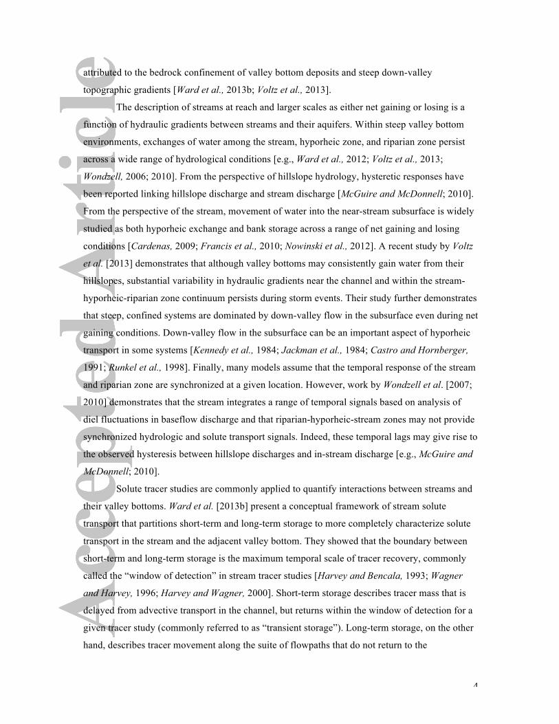
This study was completed in Watershed 1 (WS1) at the H. J. Andrews Experimental Forest,

located in the western Cascade Mountains of Oregon, United States (48○10’N, 122○15’W; Figure

1). The catchment has a steep valley gradient of 11.9% across three study reaches established for

this study and the adjacent valley width is narrow (<20m). More specifically, Figure 1B shows

the average slope of each study reach was 11.5% for the upstream reach, 16.6% for the middle

reach, and 10.1% for the downstream reach. The morphology of each reach includes a series of

pools, riffles, and steps. Each study reach was approximately 50 m in length along the valley axis,

with the downstream-most point located approximately 2 m upstream of the WS1 stream gauge

(Figure 1B). Many geomorphic features, including sediment wedges that promote large head

gradients and hyporheic exchange flows [Kasahara & Wondzell, 2003]were formed by boulders

or large, fallen trees. The catchment ranges in elevation from 421 to 1018 m above mean sea level

and has steep hillslopes (>50%) above geologically young bedrock [Swanson and James, 1975].

Valley bottom soils are shallow (1-2 m depth) loams [Dyrness, 1969] and have a documented

saturated hydraulic conductivity of 1.7 × 10-5 m s-1 [Wondzell et al., 2009]. At its outlet, the

catchment drains 95.8 ha and discharge is gauged using a permanent flume maintained by the

U.S. Forest Service. Precipitation records are from the Primary Meteorological Station at the H. J.

Andrews Experimental Forest, which is approximately 0.5 km from the catchment outlet. The

climate at the study site is characterized by wet, mild winters and dry, cool summers. Storm

6

events dominate the spring season, followed by generally dry summers and prolonged baseflow

recession. This study took place during the last major storm event before the 2011 baseflow

recession period, consisting of precipitation patterns that resulted in two storm peaks with a minor

recession between them (Figure 2). At the time of the study, the watershed was in recession from

the annual peak flow due to seasonal snowmelt runoff.

Watershed 1 contains a network of 32 shallow, small-diameter monitoring wells and

piezometers installed in 1997. Wells outside of the stream channel during baseflow were screened

over their entire length. In-stream piezometers were screened over their bottom 5-cm, with

screened sections located between 20 and 40-cm below the streambed. Further details of the well

construction and installation are summarized by Wondzell [2006], and data collection details in

these wells can be found in Voltz et al. [2013]. A sub-set of the network was instrumented with

pressure transducers to monitor the potentiometric surface at 30-minute intervals during the study

period. Additionally, in-stream pressure transducers recorded the surface-water elevation at the

intersection of well transects (oriented perpendicular to the stream) with the stream channel

(Figure 1C). Water-level observations from monitoring wells, piezometers, and in-stream loggers

were used to construct plots of hydraulic head and stream stage at two transects perpendicular to

the valley located approximately 5 m from one another (Figure 1C). Potentiometric surfaces were

plotted from piezometer and monitoring well data (Figure 3).

2.2 Solute tracer studies

Twenty-four conservative tracer slug injections were completed at each of four locations (Figure

1B) during a 9-day period (June 1-9, 2011). These injections resulted in 72 different tracer break

through curves (i.e., documented tracer concentration time series across the 3 study reach

locations). Sodium chloride (NaCl) was used as the conservative tracer, with individual tracer

slug mass ranging from 198 g to 1007 g (averaging 593 g). These tracer slug masses were scaled

to use higher masses during higher discharge conditions. Injections were located upstream of

fluid specific conductivity loggers at a distance sufficient for vertical and transverse mixing of the

tracer across the stream cross-section. The distance was scaled to have longer mixing lengths

during higher discharges [after Payn et al., 2009] and injections were made where riffles would

aid in lateral mixing. Visual approximation, an accepted practice in the field, was the chosen

method in recognition that this length would vary with discharge [e.g., Payn et al., 2009; Ward et

al., 2013b]. Although theoretical mixing lengths can be calculated, accurate discharge estimates

can be made with dilution gauging over smaller mixing lengths than those predicted by such

7

formulas [e.g., Fischer et al., 1979; Florkowski et al., 1969]. Furthermore, mixing distances may

not be well predicted by functions of channel morphology [Day, 1977].

Break through curves were logged using fluid specific electrical conductivity as a

surrogate for concentration, with dataloggers (Campbell Scientific, Logan, Utah, U.S.A.)

calibrated using a single curve based on known masses of tracer dissolved in stream water [as in,

for example, Payn et al., 2009]. No grab samples were collected during the study. Slug injections

were chosen over constant rate injection methods to characterize the rapidly changing hydrologic

conditions during the storm, and because they contain the same information as constant rate

injections for conservative tracers [e.g., Payn et al., 2008; Gooseff et al., 2008]. Prior to analysis,

background fluid electrical conductivity was subtracted from the observed time-series to isolate

the change due to the tracer from pre-tracer conditions for each breakthrough curve. Background

values for fluid electrical conductivity at the four injection locations were 38.2±1.8, 38.4±5.3,

38.6±2.7, and 40.0±5.0 µS/cm throughout the duration of the study (reported as mean ± 1

standard deviation, downstream to upstream). It was not possible to replicate tracer releases

during the storm event given the highly dynamic hydrologic conditions.

Dilution gauging is subject to several sources of error [e.g., Zellweger et al., 1989]. In

this study, high discharge observations at the downstream end of the middle study reach may

have been affected by valley geomorphology. This location is at a large bedrock outcrop, where

all down-valley subsurface flow resurfaces. Gauging at this location may have been more

sensitive to underflow than other stations that were located on alluvial deposits. Finally, dilution

gauging as applied in this study assumes steady-state discharge during the time period between

the tracer injection and the final observation of solute tracer at the monitoring point.

2.3 Long-term Storage

Solute tracer data collected in this study were analyzed using the channel water balance estimates

described by Payn et al. [2009] to evaluate long-term storage conditions. Briefly, dilution

gauging was used to calculate discharge at the downstream and upstream end of each study reach

(QU and QD, respectively), and these discharges were used to calculate a net change in discharge

for each reach, (ΔQ=QD-QU). Tracer mass loss (MLOSS) between the injection point and the

downstream end of each study reach was used to quantify gross losses. Mass loss was calculated

as

MLOSS = MIN – MREC (1)

where MIN is the known tracer mass released into the stream and MREC is the recovered tracer

mass. The MREC is calculated as

8

MREC =QD CUD dt0

t∫ (2)

where CUD is the background-corrected concentration time-series for the upstream slug at the

downstream monitoring location. Payn et al. [2009] define two end-members that bound the

range of possible behaviors in the stream. The first assumes maximum dilution of the signal (i.e.,

all gains occur before all losses) while the second assumes maximum loss of tracer (i.e., all losses

occur before all gains, defined as QLOSS,MIN and QLOSS,MAX, respectively. QLOSS,MIN and QLOSS,MAX are

calculated as

𝑄!"##,!"# =!!"##

!! ! !"!!

(3)

𝑄!"##,!"# =!!"##

!!" ! !"!!

(4)

where t is time, and CU is the background-corrected concentration time-series for the upstream

slug at the upstream monitoring location. The corresponding gross gains are calculated by mass

balance (QGAIN,MAX = ΔQ – QLOSS,MAX and QGAIN,MIN = ΔQ – QLOSS,MIN). For cases where a positive

mass loss is calculated in a net gaining segment we assume that no tracer mass was lost (i.e.,

QLOSS = 0), and assign the net change in discharge for the reach to QGAIN [after Payn et al., 2009].

For cases where interpreted gross loss is smaller than observed net loss, we assume gross loss

equals observed net loss, and zero gross gains. For cases of a positive mass loss in a net losing

stream segment, we assume the tracer results are erroneous and omit them from analysis of long-

term storage. We have not been able to identify specific sources of error in the data, nor do we

have an ability to estimate the degree to which other observations were affected by these errors.

2.4 Short-term Storage

Although a parametric approach is common when analyzing stream solute breakthrough curve

data (e.g., solving the transient storage equations of Bencala and Walters [1983]), mounting

evidence suggests this approach is limited in its ability to characterize short-term storage due to

high uncertainty and equifinality [e.g., Mason et al., 2012; Lees et al., 2000; Wagner and Harvey,

1997; Kelleher et al., In Review]. Therefore, we consider two analyses based on the observed

breakthrough curves rather than a numerical modeling framework. These analyses include

transient storage indices and temporal moment characteristics.

The window of detection is a metric that is sensitive to both the physical system and

measurement technique, and defines the boundary between short- and long-term storage [e.g.,

Harvey et al., 1996; Harvey and Wagner, 2000; Ward et al., 2013b]. We sampled tracer

9

concentration until it was indistinguishable from background concentrations in the stream. Next,

we calculated the window of detection as the time elapsed from the first detection of tracer in the

stream above background noise to the time at which 99% of the recovered solute tracer signal has

passed the observation location (hereafter t99, [after Ward et al., 2013b; Mason et al., 2012]). We

calculated the time elapsed between the observed breakthrough curve peak and t99, signifying the

time of apparent return to background tracer concentrations (hereafter the transient storage index,

or TSI, [after Mason et al., 2012]). The t99 metric does not require the assumption of any

distribution; it is calculated by trapezoidal integration of the observed time series. The TSI

provides an indicator of transient storage (information contained in the tail of the breakthrough

curve) relative to advective transport (information contained in the peak of the breakthrough

curve) [Mason et al., 2012; Harvey et al., 1996]. The TSI is calculated as:

𝑇𝑆𝐼 = 𝑡!! − 𝑡!"#$ (5).

The TSI metric may be difficult to compare across reaches or different discharge conditions

within a single reach. Therefore, we define:

TSInorm = TSI / tpeak (6).

The TSInorm metric defines the number of advective timescales elapsed between tpeak and t99, a

metric previously used by Gooseff et al. [2007] to quantify relative residence times across

multiple reaches and injections. The TSInorm metric quantifies the effect of processes other than

advection on creating late-time tailing relative to the advective timescale, providing a metric that

is independent of discharge or stream location.

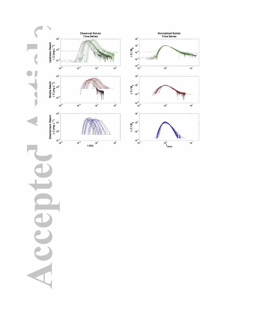
We also calculated temporal moments for the observed tracer breakthrough curves to

quantify advective transport (first temporal moment, M1), spreading (second central moment, µ2),

and tailing behavior (skewness, γ) of tracer in the study reaches [after Gupta and Cvetkovic,

2000; Schmid, 2003]. First, the normalized concentration time series (c(t)) was calculated as

𝑐 𝑡 = !!(!)

!! ! !"!!!!

(7)

where Cb(t) is the observed tracer above background levels. This normalization yields a zeroth

temporal moment (M0) of unity for all cases (i.e., the area under each breakthrough curve is one;

to remove differences due to changing slug masses and peak concentrations in-stream). Next, we

calculated nth order temporal moments (Mn) and higher order central moments (µn) as

𝑀! = 𝑐 𝑡 𝑡!!!!! 𝑑𝑡 (8), and

𝜇! = 𝑐(𝑡) 𝑡 −𝑀!!!!!

! 𝑑𝑡 (9).

Skewness was calculated by

10

(10).

Finally, we normalized t by the modal advective time in the reach (based on time elapsed

between upstream and downstream peak observations). Normalized time, tnorm, was calculated as

𝑡!"#$ = !!!"#$,!"!!!"#$,!"

(11)

where tPEAK,DS and tPEAK,US are the times at which the tracer peak passes the downstream and

upstream loggers, respectively. The effect of this normalization is that each breakthrough curve

peaks at a normalized time of one. The objective of this normalization was to compare the unique

signature of each reach on the slug injection, and eliminate variation due to different slug masses

and transport rates where transient storage across several streams with different breakthrough

curves is normalized in this manner [after Gooseff et al.; 2007]. This normalization is a

comparison of system behavior that is not confounded by changes in the advective timescale or

tracer mass. Throughout the manuscript we use the subscript “norm” in addition to variables

previously defined to denote analysis of the normalized breakthrough curve (e.g., γnorm).

2.5 ANOVA for metrics of short- and long-term storage

We analyzed metrics of short- and long-term storage for both the observed and normalized

breakthrough curves using a one-way Analysis of Variance (ANOVA). The objective of this

analysis was to determine if the metrics describing short- and long-term storage differed

significantly between the study reaches. We used a one-way ANOVA test to determine if

individual reaches were statistically different based on the experimental window of detection (t99),

long-term (channel water balance) and short-term (TSI, temporal moments) storage. As applied to

the three samples(i.e., the three study reaches) the ANOVA results indicate whether or not at least

one sample mean is drawn from a different population than the others.

3. Results

3.1 Physical Hydrology

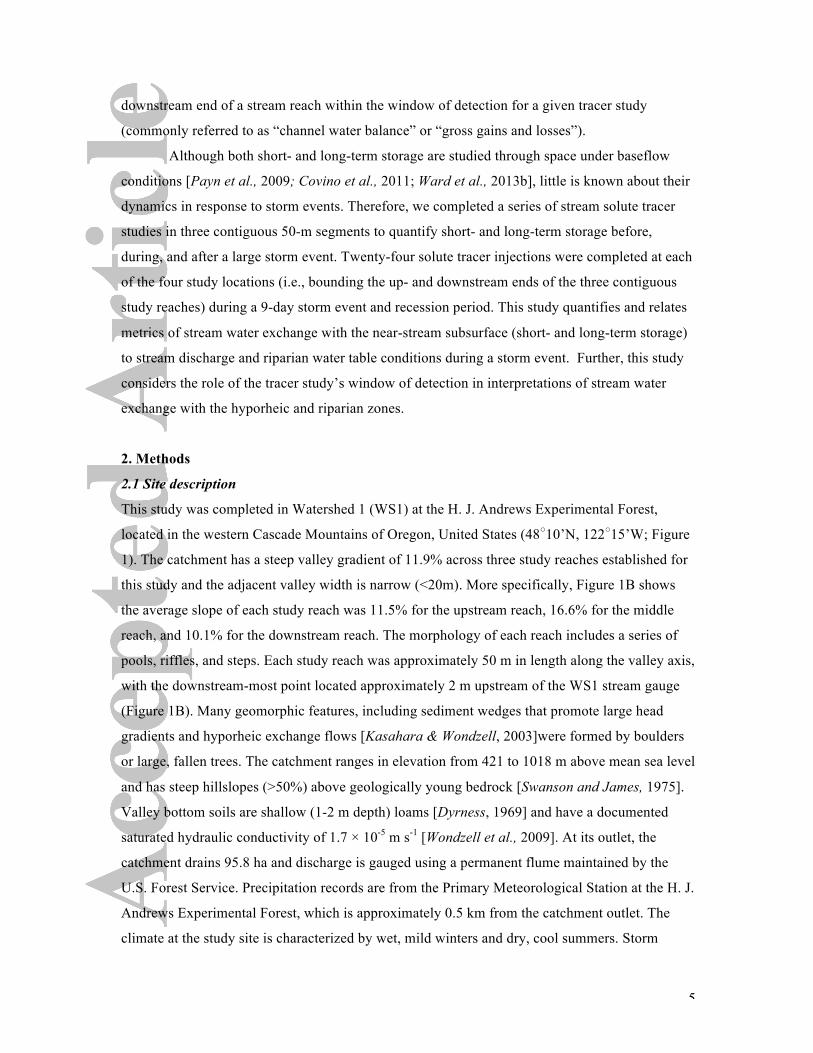
The tracer-based discharge rates agreed well with the observations made at the catchment gauge,

particularly for the lowest observed discharges (Figure 2). The largest deviations in dilution-

gauging discharge estimates from the stream-gauge discharge estimates occurred during the

highest discharge conditions (Figure 2B). The largest discharge values observed were during the

first peak of the storm event were approximately 140% and 220% of the peak value observed at

the H.J. Andrews Gauge (observed at the downstream and upstream ends of the downstream

γ =µ3µ23 2

11

study reach, respectively). For example, the dilution gauging at the two downstream-most

locations resulted in larger discharge than the gauge station at the discharge peaks (Figure 2).

Although the gauge was most recently rebuilt in 1998, the gauge is calibrated using an unknown

set of velocity rod measurements collected in the 1950s that established the stage-discharge

relationship [Henshaw, 2006] and its accuracy at these discharge rates is unknown. During this

study discharge ranged from 21.5 to 434 L s-1 at the gauge station. For water year 2010 (1-Oct-

2009 through 30-Sept-2010), the average discharge was 32.9 L s-1 (range 0.6 to 608 L s-1); the

flood of record is 2400 L s-1 [Wondzell, 2006].

Overall, the stream discharge rapidly responded to rainfall. The two rainfall events that resulted in

the hydrograph peaks represented approximately 13 cm of precipitation over a two-day period, or

a 1.25-yr return interval storm event (n=53 years) [Voltz et al., 2013]. The potentiometric surface

of the valley bottom environment was also dynamic during the study period as it responded to the

response to both rainfall on catchment hillslopes and dynamic flows in the stream. In the

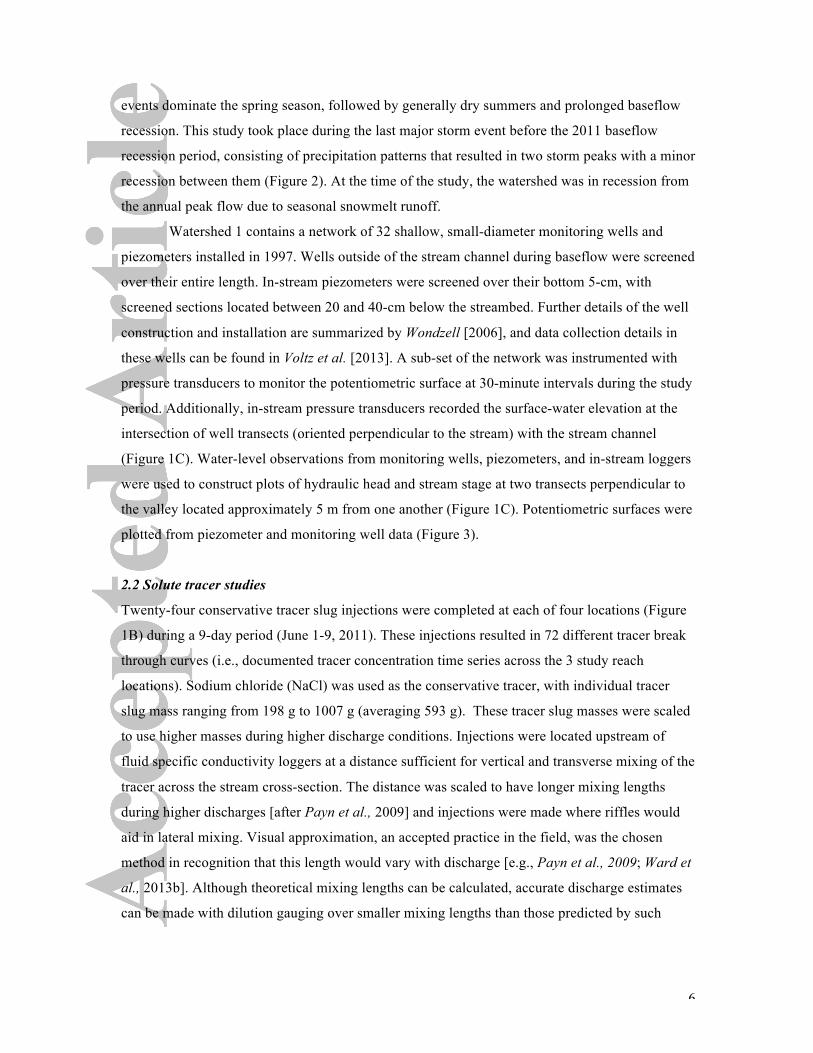
monitoring transects, the potentiometric surface rose in response to the storm events and fell after

the precipitation. At both locations, the stream gained water from the hillslope (Figure 3). The

upstream transect shows a persistent potentiometric surface below that of the stream. The

upstream transect is located where the active channel widens and the valley bottom topography is

relatively flat and has a secondary channel. In contrast, the downstream transect is at a convergent

location in the channel.

3.2 Long-term Storage

Changes in discharge at the gauge station averaged 0.46% of discharge (range 0.0% to 2.5%)

during the integration periods for individual dilution gauging measurements. Given this small

change over short timer periods we assumed the steady-state flow conditions were satisfactorily

met for individual dilution gauging events, and that our dilution gauging was valid despite the

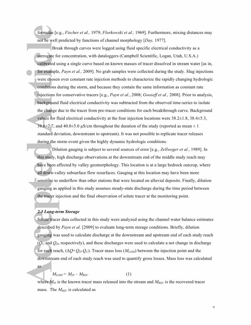
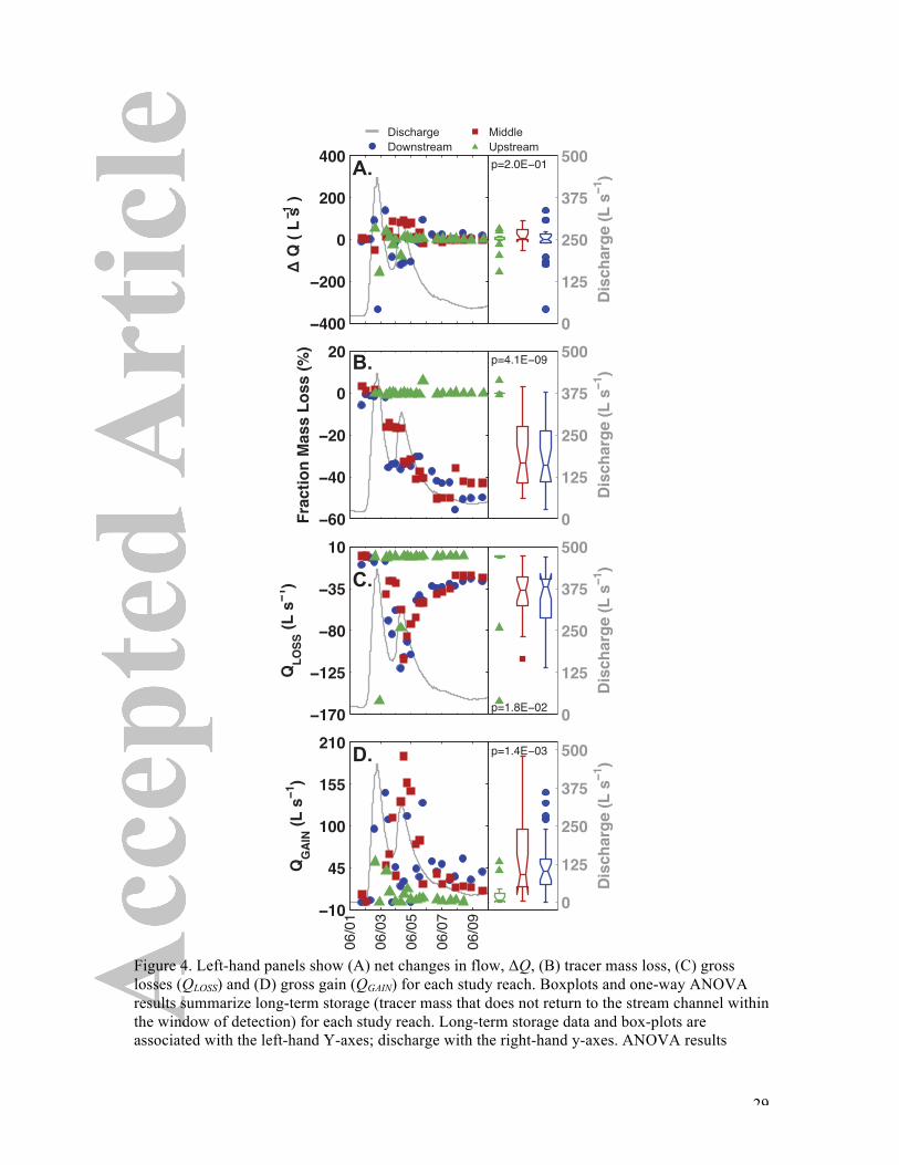
dynamics in response to rainfall. Net changes in discharge demonstrate that the stream was

generally gaining during the study period (58% of all observations), although each segment

exhibited net losing behavior during multiple discharge conditions (Figure 4A).

The fraction of slug mass lost within a given reach, a fundamental quantity used to derive

long-term storage fluxes from solute tracer data, varied in a regular pattern for most study reaches

with rising and recessional limbs of the hydrograph (Figure 4B). For 5 of the 72 tracer time

series, a positive mass loss was observed in a net losing segment and omitted from further

analysis for long-term storage. In all locations, mass losses from pre-storm conditions through the

first rising limb and about half of the first falling limb (i.e., the first five slug injections) are

12

negligible. Approximately halfway through the first falling limb, a substantial shift in tracer mass

loss was observed in the downstream and middle reaches.

During the second rising limb, mass loss remained approximately constant in each study

reach. Finally, during the second recession, mass loss in the middle and downstream reaches

slowly increased, and was approximately constant for the final 3 tracer injections. Peak changes

in the fluid electrical conductivity averaged 58.2 µS/cm (range 11.6 to 158.3 µS/cm), providing a

signal that was at least an order of magnitude above the variability in background fluid electrical

conductivity during the storm events.

We analyzed long-term storage using the frameworks of both maximum dilution (gain

before loss) and maximum tracer mass loss (loss before gains). Spatial and temporal patterns for

both were similar. We present results only for the condition of maximum dilution, as is the

practice for recent studies considering hydrologic turnover in stream networks [e.g., Covino et al.,

2011]. Gross losses of channel water remain small or zero during the first rising limb in all

reaches (Figure 4C). Gross losses in the downstream and middle reaches initially increased during

the first falling limb, and then decreased as the hydrograph reached the trough between storm

flow peaks. Losses in downstream and middle reaches increased during the second rising limb,

and then slowly decreased as the hydrograph receded to baseflow. Gross gains to the stream for

the middle and downstream reaches generally increased during the rising limbs and fell during the

receding limbs (Figure 4D). In the downstream reach, gross gains of channel water increased

briefly then decreased during the first falling limb. In the middle reach, gains slowly increased

and then decreased during the first falling limb. In all study segments, the gross gains and losses

reached a nearly constant magnitude during the second falling limb of the hydrograph, yet exhibit

varied responses during the storm event (Figures 4C, 4D).

3.3 Short-term Storage

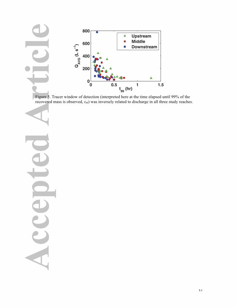
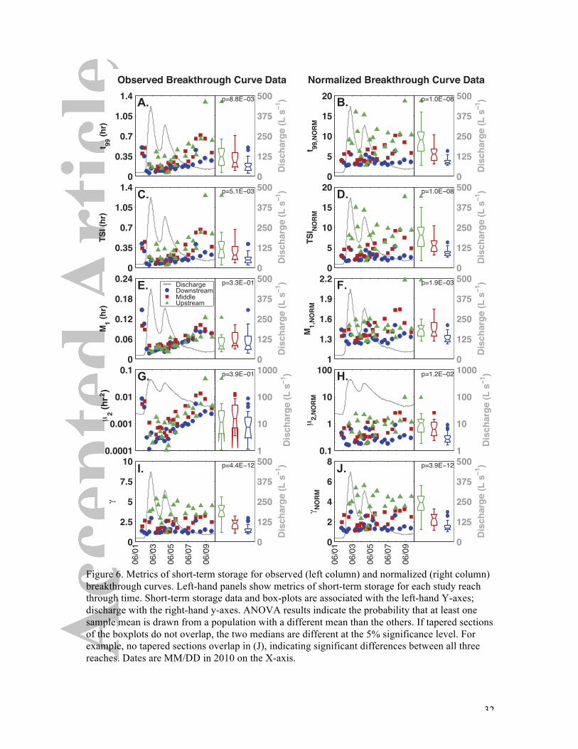
In this study, t99 varied between 0.06 and 1.3 hr for the study reaches, with maximum values

corresponding to low in-stream discharges (Figure 5 and 6A). TSI ranged from 0.043 to 1.3 hr

(mean 0.26 hr) with larger values corresponding to low in-stream discharges (Figure 6C). Small

increases in magnitudes of TSI were observed during the temporary recession in discharge

between storm peaks in the upstream and middle reaches. Mean arrival time (M1) was inversely

related to discharge with the largest values (slowest modal transport velocity) associated with the

lowest discharges (Figure 6E). Temporal variance of the tracer (µ2) decreased during the high

discharge conditions with the largest values observed during the low discharge conditions (Figure

6G). Conversely, skewness (γ) increased with discharge in the upstream reach (Figure 6I). Both

13

the middle and downstream reaches exhibited nearly constant γ throughout the study period.

These results agree with those reported by Ward et al. [2013b] along a gradient in baseflow

discharge where t99 and discharge were found to be important controls on metrics of short-term

storage.

Analysis of normalized breakthrough curves provides an assessment independent of t99

and peak concentration in-stream. For the normalized breakthrough curves, t99 is nearly constant

throughout the study period for the downstream and upstream reaches, and increased slightly in

the middle reach (Figure 6B). Both TSInorm and M1,norm exhibited similar trends (Figures 6D, 6F).

The number of advective timescales elapsed between the peak and the last detection of tracer,

TSInorm, ranged from 1.7 to 17.7 with small TSInorm values corresponding to small values of t99. In

contrast to the µ2 and γ trends for observed breakthrough curves, the normalized metrics exhibited

more constant values through time, though noise is present in the relationships (Figures 6H, 6J).

All observed and normalized solute tracer breakthrough curves are presented as supplemental

material.

3.4 Comparison of short- and long-term storage between reaches

We tested for significant differences among the different study reaches using a one-way ANOVA

for metrics of both short- and long-term storage (95% confidence level; p < 0.05 is significant;

see boxplots in Figures 4 and 6). ANOVA results, as calculated here, indicate whether or not at

least one study reach was significantly different from the others. First, we analyzed the observed

breakthrough curves. For long-term storage, the fraction of slug mass lost was significantly

different for the upstream study reach (p < 0.0001). This difference was maintained for QLOSS (p =

0.018) and QGAIN (p = 0.0014). Sample population means were not significantly different for ΔQ

(p = 0.20). For short-term storage, significant differences exist based on observed breakthrough

curves for t99 (p = 0.0088; downstream reach is significantly different), TSI (p = 0.0051;

downstream reach is significantly different), and γ (p < 0.0001; all three reaches are significantly

different from each other). No significant differences were found for M1 (p = 0.33) nor µ2 (p =

0.39). Next, we analyzed the normalized breakthrough curves, finding significant differences for

t99,norm (p < 0.0001; all three reaches are significantly different from each other), TSInorm (p <

0.0001; all three reaches are significantly different from each other), M1, norm (p = 0.0019;

downstream reach is significantly different from the other two reaches), µ2, norm (p = 0.012;

downstream reach is significantly different from the other two reaches), and γnorm (p < 0.0001; all

three reaches are significantly different from each other).

14

3.5 The window of detection as a control on interpreting short- and long-term storage

Mass losses in the upstream and middle reaches were nearly independent of t99, while the

downstream reach exhibited variability (Figure 7A). Short-term storage was strongly related to t99

throughout the storm event and recession for both the observed (left column in Figure 7) and

normalized (right column in Figure 7) breakthrough curves. TSI increases linearly with t99, with

the greatest time elapsed between the advective timescale and t99 occurring during the slowest

transport times (Figures 7C, 7D). We found increasing M1 with increasing t99 (Figures 7E, 7F).

Temporal variance (Figures 7G, 7H) and skewness (Figures 7I, 7J) increase with t99 suggesting

that processes other than advection in the stream channel (e.g., dispersion) have a greater effect

on the solute signal when they have more time to act on that signal. If the spreading and tailing

are attributed to hyporheic exchange, this suggests the observable timescales of subsurface

processes are primarily affected by the advective velocity of the stream.

4. Discussion

4.1 Linking short- and long-term storage with valley bottom hydrology

There was little variation in the direction of riparian hydraulic gradients lateral to the valley

bottom throughout the storm events of this study (Figure 3, Upstream Transect). Persistent losing

conditions observed at the upstream transect are inconsistent with the conceptual models that

predict increasing hydraulic gradients toward the stream during storm events and suppressing

hyporheic flow [Hakenkamp et al., 1993; Hynes, 1983; Meyer et al., 1988; Palmer, 1993; Vervier

et al., 1992; White, 1993]. The stream appears to always lose water to the subsurface in some

locations, even when the stream stage is rising (Figure 3, Upstream Transect). We interpret this as

evidence of persistent hyporheic exchange driven by local geomorphology, and as a simultaneous

gain of water from the hillslope and loss of water along hyporheic flowpaths from the stream

channel perspective.

Previous studies in the same watershed also demonstrate that this valley-bottom

hydrology behavior is not unique to this study or event [see Voltz et al., 2013; Wondzell, 2006;

2010]. Voltz et al. [2013] showed in detail that the gradients in and adjacent to the stream channel

change very little in response to the storm events in the highly instrumented section of the middle

reach (Figure 1C). Their study further found that most locations in the WS1 valley bottom were

dominated by down-valley hydraulic gradients (parallel to the stream) as opposed to cross-valley

gradients (perpendicular to the stream) upon which the majority of current conceptual models are

based. During the storm event, Voltz et al. [2013] report that near-stream hydraulic gradients in

15

some locations even turn away from the stream channel, increasing the movement of water and

tracer from the stream to the aquifer.

We hypothesize the persistent hyporheic flowpaths observed at the upstream transect in

the present study (Figure 3) are due to the location of this transect near a riffle and widening

section of the valley bottom. In a nearby steep mountain catchment (Watershed 3, < 1km from

WS1 in the HJ Andrews Experimental Forest), Ward et al. [2012] found that the physical extent

of stream water in the aquifer during baseflow recession was largely invariant, and that

geomorphology was the primary control on stream-aquifer interactions in this system. There is a

growing body of literature suggesting that valley-bottom geology and near surface morphology

(e.g., hillslopes, valley bottom width, underlying bedrock profile and alluvial deposit depth) are

the dominant controls on stream-aquifer interactions in steep headwater streams [e.g., Kasahara

and Wondzell, 2003; Wondzell 2006, 2010; Payn et al., 2012; Ward et al., 2012; 2013a]. The

present study suggests that geomorphology of the individual stream reaches in combination with

the hillslopes discharging to the valley bottom modifies solute tracer timeseries in a predictable

way, scaled by the overall advective travel time in the reach. The magnitude of metrics describing

the short-term storage increases with increasing t99; for example, skewness grows with increasing

t99 because there is more time for processes other than advection to act on the signal.

Conceptually, experiments with larger t99 should exhibit increased µ2 and γ, because

short-term storage processes would have more time to act on the solute tracer signals. The novel

storm-event data from this study confirm this relationship for both observed and normalized

breakthrough curves (Figure 7). For longer advective timescales, we found longer mean travel

times (Figures 7E, 7F). Positive relationships between t99 and higher-order central moments

(Figures 7F, 7G, 7H, 7I) suggest that increased short-term storage (evidenced by increased

spreading and asymmetric tailing) occurs during the lowest discharge conditions. These t99

patterns are also a function of the channel hydraulics controlled by the geomorphology of the

valley bottom. However, we posit that the different slopes observed between γ and t99 are

indicative of changes in the stream and valley bottom morphology. For example, the relationship

between discharge and channel structure in the upstream reach may allow the active stream

channel to temporarily access portions of the riparian valley bottom that include many roughness

elements, that increase surface transient storage (e.g., fallen logs, debris jams, shrubs and

grasses). We attribute the incorporation of these elements into the active channel as the source of

the observed relationship between t99 and γ surface transient storage. Inherent in this attribution is

that these storage processes affect transient storage (indicated by a larger γ), but not advection nor

longitudinal dispersion (which would appear in values for M1 and µ2, respectively).

16

4.2 Stream reaches provide characteristic modification to solute signals independently of in-

stream discharge rate

The first major precipitation event caused a shift in long-term storage that did not return to pre-

storm conditions during the study. While hysteretic behavior of hillslope-riparian-stream

interactions has been reported [e.g., McGlynn and McDonnell, 2003; McGlynn et al., 2004;

McGuire and McDonnell; 2010], these studies have not been extended to account for the behavior

within the riparian and hyporheic zones. This shift in long-term storage is particularly evident in

the patterns in mass loss, where the middle and downstream reaches show increasing mass loss

during the storm event and its recession. These mass losses represent substantial increases in

QLOSS and corresponding increases in QGAIN during the second peak of the storm event.

Furthermore, the storm caused a shift in short-term storage interpreted from recovered in-stream

tracer. The valley-bottom hydrology was not highly dynamic during the storm event based on

ground water elevations alone. However, with the evidence of the tracer studies, it is clear that

both short- and long-term storage were highly variable during the storm events. Thus, the

exchange of water between streams and their aquifers is highly dynamic during storm events and

may not be apparent to investigations solely relying on valley-bottom ground water elevations.

No notable, irreversible changes in the physical morphology of the system were observed during

the storm event (e.g., hillslope failures, log falls) to explain this change in storage. Changes in

stage did result in different extents of the valley bottom becoming active parts of the channel

during the different periods of the study.

In WS1 and across a large range of discharges, the normalized breakthrough curves

showed that each of the study reaches imparted a unique modification to the injected solute tracer.

.While there is not a ubiquitous correlation of all normalized breakthrough curves at an individual

reach, we found unique storage modifications within each reach that were significantly different

from one another. This is similar to storage dynamics observed by Zarnetske et al., [2007], who

concluded that unique reach morphologies can act as stronger modifiers of water storage

dynamics than orders-of-magnitude variability in discharge. Further, the observed relationships

between discharge and all short-term storage metrics suggests that the same suite of flowpaths is

affecting the in-stream solute signal during all flow conditions, because the effect of these

flowpaths on the tracer signal varies as a function of t99 (i.e., the window of detection for each

tracer study). More formally, the process domain (i.e., the region in space and time over which

the morphologic structure of the stream influences stream hydraulics [Montgomery, 1999]) is

nearly constant through space and time based on our normalized solute tracer data. The

17

combination of morphology and discharge are unique to each tracer study and gives rise to a

unique window of detection, which confounds the interpretation of short- and long-term storage

in our study and others [e.g., Ward et al., 2013b; Drummond et al., 2012].

4.3 A dynamic perceptual model of the hillslope-riparian-hyporheic-stream continuum

To explain observed metrics of short- and long-term storage, we pose a 3-D, dynamic, perceptual

model as an explanation of the observed patterns of metrics describing short- and long-term

storage that were observed in this study. The perceptual model is a qualitative representation of

dominant processes that are critical to a description of hydrological system response, and is based

on subjective understanding of hydrological processes occurring at the field site [e.g. Sivapalan,

2003; Wagener et al., 2007]. We present our perceptual model of the WS1 hillslope-riaparian-

hyporheic-stream continuum to explain the field observations that do not fit within existing

conceptual models. Further this conceptual mode serves to integrate our understanding of the

hydrological processes in the sense of, for example, McGlynn et al. [1999], acknowledging that

continued study is often coupled with refinement and revision of such perceptual models

[McGlynn et al., 2002]. Although the perceptual model includes the major drivers and feedbacks

of the system, the magnitudes of each are expected to be heterogeneous in space (e.g., between

study reaches).

Our perceptual model of WS1 represents the pre-storm through recession limb period

captured by this study, and the variable flow conditions across the hillslope-riparian-hyporheic-

stream continuum (Figure 8). As the first storm event occurs and the initial rising limb develops

in the stream, the riparian zone responds rapidly, compressing hyporheic flowpath networks and

creating generally gaining conditions evidenced by the low mass loss in all reaches during the

pre-storm and first rising limb (Figure 8C). Following the cessation of the first storm event and

during the first falling limb (Figure 8D), the hydraulic gradients from the hillslope and riparian

zone to the stream decrease (Figure 3), allowing increased lateral extent of hyporheic flowpaths

and increased tracer mass loss. The down-valley underflow increases as a result of the catchment

response to the precipitation, because the hillslopes begin discharging to the riparian zone, which

is dominated by down-valley hydraulic gradients in WS1 [Voltz et al., 2013]. Across the variable

flow conditions, the mass lost from the stream channel is more likely to remain in underflow

rather than return to the stream, which explains the increased mass loss during the first falling

limb of the study (Figure 2). During the rising limb of the second precipitation event (Figure 8E),

the hillslopes and riparian zones (with increased antecedent moisture levels due to the first

precipitation event) respond rapidly, increasing hydraulic gradients toward the stream. This

18

compresses hyporheic exchange pathways in accordance with several existing conceptual models

[e.g., Hynes, 1983; Meyer et al., 1988; Vervier et al., 1992; Hakenkamp et al., 1993; Palmer,

1993; White, 1993]. and explains the plateau in tracer mass loss (Figure 4). During the second

rising limb the underflow is maintained [Voltz et al., 2013], transporting tracer lost from the

stream down-valley in the aquifer, and eventually returning the flow and tracer to the stream

downstream of the study reach. Finally, following the cessation of the second storm event (Figure

8F), the hydraulic gradients from the hillslope to stream relax, allowing the expansion of the

hyporheic zone. The underflow remains high during this second recession period, because the

upstream catchment is still relaxing back to pre-storm conditions and discharging to this

convergent location near the catchment outlet. This extended relaxation period explains why the

observed tracer behavior does not return to pre-storm conditions (e.g., very low tracer mass loss)

during our study period despite the return of discharge to pre-storm magnitudes (Figure 2).

5. Conclusions

We collected a unique data set of conservative solute tracer transport before, during, and after a

major storm event in a headwater mountain stream. These data characterize both short- and long-

term storage in the stream and reveal an improved understanding of how water and solutes move

through the stream network during storm events. The tracer tests provide evidence of short- and

long-term storage, both representing some amount of interaction between the stream and

groundwater at the reach-averaged scale. We use a variety of metrics to describe the solute tracer

breakthrough curves (e.g., TSI, t99), and we note here that these are descriptors only; that do not

isolate cause-effect relationships for watershed processes and storage dynamics. Further, the

observations of the valley-bottom head gradients alone indicate magnitudes and directions of

exchange, but are limited in space. The interpretations of tracer tests alone are complicated

because they span a range of spatial scales. However, both tracer studies and water table

observations demonstrate dynamic hydrological fluxes during storm events. Given that

hydrodynamics are recognized as a significant control on biological and chemical systems in

streams and their ground waters [after Battin, 1999; 2000; Zarnetske et al., 2011; Ward et al.,

2011], the decrease of t99 with increasing discharge suggests a decreased potential for hyporheic

and riparian biogeochemical cycling to affect in-stream signatures. It is unlikely that static

conceptual models are sufficient to explain the sources of observed in-stream biological and

chemical processes during dynamic flow conditions. Therefore, we developed a new conceptual

model for the dynamics of hillslope-riparian-hyporheic-stream continuum at the site across storm

events. Still, further work is needed, because neither technique in this study nor the combination

19

of them fully captures the time-variable 3-D exchanges occurring between the stream and its

aquifer across the range of spatial and temporal scales.

Overall, this study demonstrates that: (1) metrics of short- and long-term storage were

highly variable with stream discharge, largely due to variation in the tracer-based window of

detection; (2) characteristic modifications of solute tracer signals exist in different study reaches

independent of stream discharge and can be predominantly controlled by valley-bottom

morphology; (3) localized losing conditions were consistently observed in certain locations even

during the rising limb of the storm hydrograph, demonstrating local hyporheic flowpaths that

persist through strongly gaining conditions at the valley-bottom scale; (4) short- and long-term

storage are complimentary descriptions of stream water and solute transport, partitioned by the

window of detection; (5) stream discharge responds to storm events and recovers from them over

a shorter timescale than metrics of short- and long-term storage recover; (6) the exchange of

water between streams and their aquifers is highly dynamic during storm events and may not be

apparent to investigations solely relying on valley-bottom ground water elevations; and (7) down-

valley flux in the subsurface is an important component of stream-aquifer interactions that is not

represented in many conceptual models of riparian hydrology. Understanding the fate of water

and solutes in headwater streams requires in-depth understanding of riparian zone hydrology.

Short- and long-term storage are complementary processes that define how solute signals at the

upstream end of a reach are translated to the downstream end, with implications for solute fate

and transport at the network scale.

20

Acknowledgments

Research facilities, precipitation data, and flow gauge data were provided by the H.J. Andrews

Experimental Forest research program, funded by the National Science Foundation’s Long-Term

Ecological Research Program (DEB 08-23380), US Forest Service Pacific Northwest Research

Station, and Oregon State University. This manuscript is based upon work supported by the

National Science Foundation’s Hydrologic Sciences program, under grant no. EAR-0911435. JZ

acknowledges additional support from the Yale Institute for Biospheric Studies. Any opinions,

findings, and conclusions or recommendations expressed in this material are those of the authors

and do not necessarily reflect the views of the National Science Foundation or the H.J. Andrews

Experimental Forest. The authors thank the reviewers for constructive feedback that improved the

quality of this manuscript.

21

References: Battin, T. (1999), Hydrologic flow paths control dissolved organic carbon fluxes and metabolism

in an alpine stream hyporheic zone, Water Resources Research., 35(10), 3159–3169, doi:10.1029/1999WR900144.

Battin, T. (2000), Hydrodynamics is a major determinant of streambed biofilm activity: From the sediment to the reach scale, Limnol. Oceanogr.,45, 1308–1319, doi:10.4319/lo.2000.45.6.1308.

Bencala, K., and R. Walters (1983), Simulation of solute transport in a mountain pool-and-riffle stream: a transient storage model, Water Resources Research, 19(3), 718-724.

Boulton, A. J., S. Findlay, P. Marmonier, E. H. Stanley, and H. M. Valett (1998), The functional significance of the hyporheic zone in streams and rivers, Annual Reviews in Ecology and Systematics, 29(1), 59-81.

Boulton, A. J., T. Datry, T. Kasahara, M. Mutz, and J. A. Stanford (2010), Ecology and management of the hyporheic zone: stream-groundwater interactions of running waters and their floodplains, Journal of the North American Benthological Society, 29(1), 26-40.

Brunke, M., and T. Gonser (1997), The ecological significance of exchange processes between rivers and groundwater, Freshwater Biology, 37, 1-33.

Cardenas, M. B. (2009), Stream-aquifer interactions and hyporheic exchange in gaining and losing sinuous streams, Water Resources Research, 45, W06429.

Castro, N. M., and G. M. Hornberger (1991), Surface-subsurface water interactions in a alluviated mountain stream channel, Water Resources Research, 27(7), 1613-1621.

Covino, T., B. L. McGlynn, and J. Mallard (2011), Stream-groundwater exchange and hydrologic turnover at the network scale, Water Resources Research, 47(12), W12521.

Day, T. (1977), Field procedures and evaluation of a slug dilution gauging method in mountain streams, Journal of Hydrology (New Zealand), 16(2), 113-133.

Drummond, J., T.P. Covino, A. Aubeneu, D. Leong, S. Patil, R. Schumer, and A. Packman (2012) Effects of Solute Breakthrough Curve Tail Truncation on Residence Time Estimates: A Synthesis of Solute Tracer Injection Studies. Journal of Geophysical Research: Biogeosciences. 117, G00N08.

Duval, T., and A. Hill (2006), Influence of stream bank seepage during low-flow conditions on riparian zone hydrology, Water Resources Research, 42(10), W10425.

Dyrness, C. (1969), Hydrologic properties of soils on three small catchments in the western Cascades of Oregon, USDA FOREST SERV RES NOTE PNW-111, SEP 1969. 17 P.

Fischer, H. B., E. J. List, R. C. Y. Koh, J. Imberger, N. H. Brooks (1979), Mixing in Inland and Coastal Waters, Academic Press, San Diego, California, USA.

Florkowski, T., T. G. Davis, B. Wallander, and D. R. L. Prabhakar (1969), The measurement of high discharges in turbulent rivers using tritium tracer, Journal of Hydrology, 8, 248-261.

Francis, B. A., L. K. Francis, and M. B. Cardenas (2010), Water table dyamics and groundwater- surface water interactions during filling and draining of a large fluvial island due to dam- induced river stage fluctuations, Water Resources Research, 46, W07513.

Gooseff, M. N., S. M. Wondzell, R. Haggerty, J. Anderson (2003), Comparing transient storage modeling and residence time distribution (RTD) analysis in geomorphically varied reaches in the Lookout Creek basin, Oregon, USA, Advances in Water Resources, 26, 925-937.

Gooseff, M. N., R. O. Hall Jr., J. L. Tank (2007), Relating transient storage to channel complexity in streams of varying land use in Jackson Hole, Wyoming, Water Resources Research, 43, W01417. doi:10.1029/2005WR004626.

Gooseff, M. N., R. A. Payn, J. P. Zarnetske, W. B. Bowden, J. P. McNamara, and J. H. Bradford (2008), Comparison of in-channel mobile-immobile zone exchange during instantaneous and constant rate stream tracer additions: Implications for design and interpretation of non-conservative tracer experiments, Journal of Hydrology, 357(1-2), 112-124.

22

Gu, C., Hornberger, G.M., Mills, A.L., and J.S. Herman 2008. Influence of stream-aquifer interactions in the riparian zone on NO3- flux to a low-relief coastal stream, Water Resources Research. 44: W11432, doi:10.1029/2007WR006739

Gupta, A., and V. Cvetkovic (2000), Temporal moment analysis of tracer discharge in streams: combined effect of physicochemical mass transfer and morphology, Water Resources Research, 36(10), 2985-2997.

Hakenkamp, C. C., H. M. Valett, A. J. Boulton (1993), Perspectives on the hyporheic zone: Integrating hydrology and biology. Concluding remarks, Journal of the North American Benthological Society, 12(1), 94-99.

Hancock, P. J. (2002), Human impacts on the stream-groundwater exchange zone, Environmental Management, 29(6), 763-781.

Harvey, J., and K. Bencala (1993), The effect of streambed topography on surface-subsurface water exchange in mountain catchments, Water Resources Research, 29(1), 89-98.

Harvey, J. W., B. J. Wagner, and K. E. Bencala (1996), Evaluating the reliability of the stream tracer approach to characterize stream-subsurface water exchange, Water Resources Research, 32(8), 2441-2451.

Harvey, J. W., and B. J. Wagner (2000), Quantifying hydrologic interactions between streams and their subsurface hyporheic zones, in Streams and Ground Waters, edited by J. B. Jones and P. J. Mulholland, pp. 3–44.

Henshaw, D. (2006). Andrews Forest Streamflow Calculation and Rating Curve Summary. Available online at http://andrewsforest.oregonstate.edu/data/studies/hf04/rating_curve_history.pdf. Accessed 30-July-2012.

Hynes, H. (1983), Groundwater and stream ecology, Hydrobiologia, 100(1), 93-99. Jackman, A. P., R. A. Walters, V. C. Kennedy (1984), Transport and concentration controls for

chloride, strontium, potassium and lead in Uvas Creek, a small cobble-bed stream in Santa Clara County, California, USA: 2. Mathematical modeling, Journal of Hydrology, 75(1-4), 111-141.

Jencso, K. G., B. L. McGlynn, M. N. Gooseff, K. E. Bencala, S. M. Wondzell (2010), Hillslope hydrologic connectivity controls riparian groundwater turnover: Implications of catchment structure for riparian buffering and stream water sources, Water Resources Research, 46, W10524.

Jencso, K. G., and B. L. McGlynn (2011), Hierarchical controls on runoff generation: Topographically driven hydrologic connectivity, geology, and vegetation, Water Resources Research., 47(11), W11527.

Kasahara, T. and S. M. Wondzell (2003), Geomorphic controls on hyporheic exchange flow in mountain streams, Water Resources Research., 39(1), doi:10.1029/2002WR001386

Kelleher, C.A., T. Wagener, B. L. McGlynn, A. S. Ward, M.  N.  Gooseff,  and  R.  A.  Payn  (In   Review)  Stream  characteristics  govern  the  importance  of  transient  storage   processes,  Water  Resources  Research.

Kennedy, V. C., A. P. Jackman, S. M. Zand, G. W. Zellweger, and R. J. Avanzino (1984), Transport and concentration controls for chloride, strontium, potassium and lead in Uvas Creek, a small cobble-bed stream in Santa Clara County, California, USA: 1. Conceptual model, Journal of Hydrology, 75(1-4), 67-110.

Krause, S., D. M. Hannah, J. H. Fleckenstein, C. M. Heppell, D. Kaeser, R. Pickup, G. Pinday, A. L. Robertson, P. J. Wood (2011), Inter‐disciplinary perspectives on processes in the hyporheic zone, Ecohydrology, 4(4), 481-499.

Larkin, R. G., and J. M. Sharp (1992), On the relationship between river-basin geomorphology, aquifer hydraulics, and ground-water flow direction in alluvial aquifers, Bulletin of the Geological Society of America, 104(12), 1608-1620.

Lees, M., L. A. Camacho, and S. Chaptra (2000), On the relationship of transient storage and

23

aggregated dead zone models of longitudinal solute transport in streams, Water Resources Research, 36(1), 213-224.

Mason, S. J. K., B. L. McGlynn, and G. C. Poole (2012), Hydrologic response to channel reconfiguration on Silver Bow Creek, Montana, Journal of Hydrology, 438-439, 125-136.

McGlynn, B. L. and J. J. McDonnell (2003), Quantifying the relative contributions of riparian and hillslope zones to catchment runoff, Water Resources Research, 39(11).

McGlynn, B. L., J. J. McDonnel, and D. D. Brammer (2002), A review of the evolving perceptual model of hillslope flowpaths at the Maimai catchments, New Zealand, Journal of Hydrology, 257, 1-26.

McGlynn, B. L., J. J. McDonnel, J. Seibert, and C. Kendall (2004), Scale effects on headwater catchment runoff timing, flow sources, and groundwater-streamflow relations, Water Resources Research, 40, W07504.

McGlynn, B.L., J. J. McDonnel, J. B. Shanley, and C. Kendall (1999), Riparian zone flowpath dynamics during snowmelt in a small headwater catchment, Journal of Hydrology, 222, 75-92.

McGuire, K. J., and J. J. McDonnel (2010), Hydrological connectivity of hillslopes and streams: Characteristic time scales and nonlinearities, Water Resources Research, 46, W10543.

Meyer, J. L., W. H. McDowell, T. L. Bott, J. W. Elwood, C. Ishizaki, J. M. Melack, B. L. Peckarsky, B. J. Peterson, and P. A. Rublee (1988), Elemental dynamics in streams, Journal of the North American Benthological Society, 7(4), 410-432.

Montgomery, D. R. (1999), Process domains and the river continuum, Journal of the American Water Resources Association, 35(2), 397-410.

Nowinski, J. D., M. B. Cardenas, A. F. Lightbody, T. E. Swanson, and A. H. Sawyer (2012), Hydraulic and thermal response of groundwater-surface water exchange to flooding in an experimental aquifer, Journal of Hydrology, 472-473, 184-192.

Palmer, M. A. (1993), Experimentation in the hyporheic zone: challenges and prospectus, Journal of the North American Benthological Society, 12(1), 84-93.

Payn, R. A., M. N. Gooseff, D. A. Benson, O. A. Cirpka, J. P. Zarnetske, W. B. Bowden, J. P. McNamara, andJ. H. Bradford (2008), Comparison of instantaneous and constant-rate stream tracer experiments through non-parametric analysis of residence time distributions, Water Resour. Res., 44, W06404, doi:10.1029/2007WR006274.

Payn, R., R. A., M. N. Gooseff, B. L. McGlynn, K. E. Bencala, and S. M. Wondzell (2009), Channel water balance and exchange with subsurface flow along a mountain headwater stream in Montana, United States, Water Resources Research, 45.

Payn, R. A., M. N. Gooseff, B. L. McGlynn, K. E. Bencala, and S. M. Wondzell (2012), Exploring changes in the spatial distribution of stream baseflow generation during a seasonal recession, Water Resources Research., 48, W04519.

Poole, G. C. (2002), Fluvial landscape ecology: addressing uniqueness within the river discontinuum, Freshwater Biology, 47, 641-660.

Runkel, R. L., D. M. McKnight, and E. D. Andrews (1998), Analysis of transient storage subject to unsteady flow: diel flow variation in an Antarctic stream, Journal of the North American Benthological Society, 17(2), 143-154.

Schmid, B. H. (2003), Temporal moments routing in streams and rivers with transient storage, Advances in Water Resources, 26(9), 1021-1027.

Shibata, H., O. Sugawara, H. Toyoshima, S. M. Wondzell, F. Nakamura, T. Kasahara, F. J. Swanson, and K. Sasa (2004), Nitrogen dynamics in the hyporheic zone of a forested stream during a small storm, Hokkaido, Japan, Biogeochemistry, 69, 83-104.

Sivapalan, M. (2003), Process complexity at hillslope scale, process simplicity at the watershed scale: is there a connection?, Hydrological Processes, 17, 1037-1041.

24

Stanford, J. A., and J. V. Ward (1993), An ecosystem perspective of alluvail rivers: Connectivity and the hyporheic corridor, Journal of the North American Benthological Society, 12(1), 48-60.

Swanson, F. J., and M. E. James (1975), Geology and geomorphology of the H.J. Andrews Experimental Forest, western Cascades, Oregon, Res. Pap. PNW‐188, Pac. Northwest For. and Range Exp. Stn., For. Serv., U.S. Dep. of Agric., Portland, Oreg.

Triska, F. J., et al. (1990), In situ retention-transport response to nitrate loading and storm discharge in a third-order stream, Journal of the North American Benthological Society, 9(3), 229-239.

Vervier, P., J. Gibert, P. Marmonier, M.J. Dole-Oliver (1992), A perspective on the permeability of the surface freshwater-groundwater ecotone, Journal of the North American Benthological Society, 11(1), 93-102.

Voltz, T.J., M. N. Gooseff, A. S. Ward, K. Singha, M. Fitzgerald, T. Wagener (2013), Riparian hydraulic gradient and stream-groundwater exchange dynamics in steep headwater valleys, JGR-Earth Surface, 118, doi:10.1002/jgrf.20074.

Wagener, T., M. Sivapalan, P. Troch, R. Woods (2007), Catchment Classification and Hydrologic Similarity, Geography Compass, 1(4), 901-931.

Wagner, B., and J. W. Harvey (1997), Experimental design for estimating parameters of rate- limited mass transfer: Analysis of stream tracer studies, Water Resources Research, 33(7), 1731-1741.

Ward, A. S., M. N. Gooseff, and P. A. Johnson (2011), How can subsurface modifications to hydraulic conductivity be designed as stream restoration structures? Analysis of Vaux’s conceptual models to enhance hyporheic exchange, Water Resources Research., 47, W08512, doi:10.1029/2010WR010028.

Ward, A. S., M. N. Gooseff, and K. Singha, (2013a), How Does Subsurface Characterization Affect Simulations of Hyporheic Exchange? Ground Water, 51: 14–28

Ward, A. S., M. N. Gooseff, M. Fitzgerald, T. J. Voltz, A. M. Binley, and K. Singha (2012), Hydrologic and geomorphic controls on hyporheic exchange during base flow recession in a headwater mountain stream, Water Resources Research, 48(4), W04513.

Ward, A. S., R. A. Payn, M. N. Gooseff, B. L. McGlynn, K. E. Bencala, C. A. Kelleher, S. M. Wondzell, and T. Wagener (2013b), Interpretation of stream solute tracer studies to describe hydrological organization of short- and long-term storage along a stream, Water Resources Research, 49, doi:10.1002/wrcr.20148.

White, D. S. (1993), Perspectives on defining and delineating hyporheic zones, Journal of the North American Benthological Society, 12(1), 61-69.

Woessner, W. W., 2000, Stream and fluvial plain ground-water interactions: re-scaling hydrogeologic thought. Ground Water, 38 (3), p. 423-429. Wondzell, S. (2006), Effect of morphology and discharge on hyporheic exchange flows in two small streams in the Cascade Mountains of Oregon, USA, Hydrological Processes, 20(2), 267-287.

Wondzell, S. (2006), Effect of morphology and discharge on hyporheic exchange flows in two small streams in the Cascade Mountains of Oregon, USA, Hydrological Processes, 20(2), 267-287.

Wondzell, S. M., M. N. Gooseff, B. L. McGlynn (2010), An analysis of alternative conceptual models relating hyporheic exchange flow to diel fluctuations in discharge during baseflow recession, Hydrological Processes, 24(6), 686-694.

Wondzell, S. M., M. N. Gooseff, B. L. McGlynn (2007), Flow velocity and the hydrologic behavior of streams during baseflow, Geophysical Research Letters, 34, 24.

Wondzell, S. M., J. LaNier, R. Haggerty (2009), Evaluation of alternative groundwater flow models for simulating hyporheic exchange in a small mountain stream, Journal of Hydrology, 364(1-2), 142-151.

25

Wondzell, S.M. and F. J. Swanson (1996), Seasonal and storm dynamics of the hyporheic zone of a 4th-order mountain stream. I: Hydrologic Processes, Journal of the North American Benthological Society, 15(1), 3-19.

Zarnetske, J.P., M.N. Gooseff, W.B. Bowden, T.R. Brosten, J.H. Bradford, and J.P. McNamara (2007), Transient storage as a function of geomorphology, discharge, and permafrost active layer conditions in Arctic tundra streams, Water Resources Research., 43, W07410, doi:10.1029/2005WR004816.

Zarnetske, J.P., R. Haggerty, S.M. Wondzell, and M.A. Baker (2011), Dynamics of nitrate production and removal as a function of residence time in the hyporheic zone. J. Geophys. Res., 116, G01025, doi:10.1029/2010JG001356.

Zarnetske, J.P., R. Haggerty, S.M. Wondzell, V. Bokil, and R. González-Pinzón (2012), Coupled transport and reaction kinetics control the nitrate source-sink function of hyporheic zones. Water Resources Research., 48, doi:10.1029/ 2012WR011894.

Zellweger, G. W., R. J. Avanzino, and K. E. Bencala (1989), Comparison of tracer-dilution and current-meter discharge measurements in a small gravel-bed stream, Little Lost Man Creek, California, U.S. Geol. Surv. Water Resour. Invest. Rep., 89–4150.

26

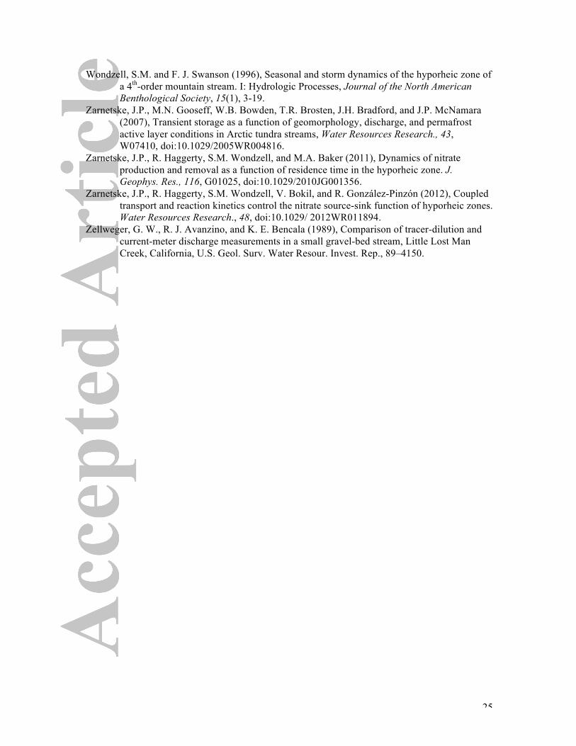
Figure 1. (A) Topography for the study catchment. (B) Profile along the stream centerline for our three study reaches, and (C) Plan-view of the monitoring network in the middle study reach where water table elevations were observed.

450

449446

447448

445

444443

442

0 6 12 183

Meters

Well

Stream Stage

PiezometerRiparian Zone

Gauge

Stream

Elevation (m)1018

421

Meters0 105 210 420 630 840

0 50 100 150435

440

445

450

455

460

Distance from Gauge (m)

Elev

atio

n (m

)

Downstream ReachMiddle ReachUpstream Reach

A.

B.

C.

Figure 1C

Figure 1B

Stream Extent

HillslopeThalweg

Contour

27

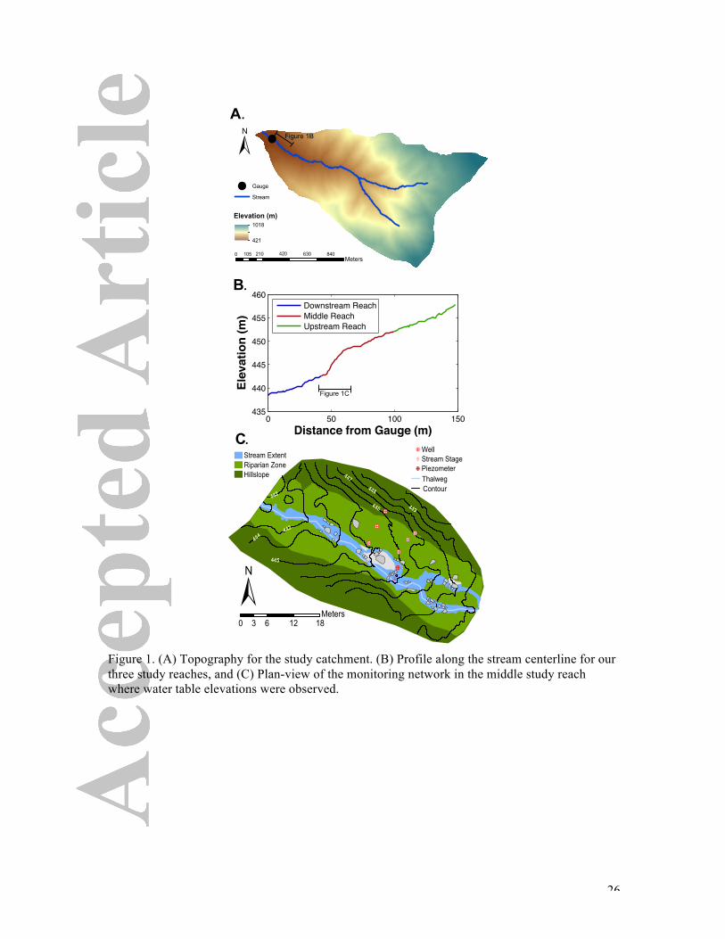
Figure 2. (A) Seasonal discharge from WS1 at the H.J. Andrews Experimental Forest. (B) Precipitation and discharge during the study period. Dilution gauging at four points bounded the upstream and downstream end of each study segment, with the downstream monitoring location immediately upstream of a permanently installed gauge station. Dates are MM/DD in 2010. The color scheme presented here is used for all subsequent figures in the manuscript.

012Ho

urly

Prec

ip.(m

m)

06/01 06/02 06/03 06/04 06/05 06/06 06/07 06/08 06/09 06/100

200400600800

Disc

harg

e (L

s!1)

H.J. Andrews GaugeDownstream EndDownstream!Middle TransitionMiddle!Upstream TransitionUpstream End

03/01 04/01 05/01 06/01 07/01 08/01 09/01

0.11

10100

1000Di

scha

rge

(L s!1

)

A.

B.

28

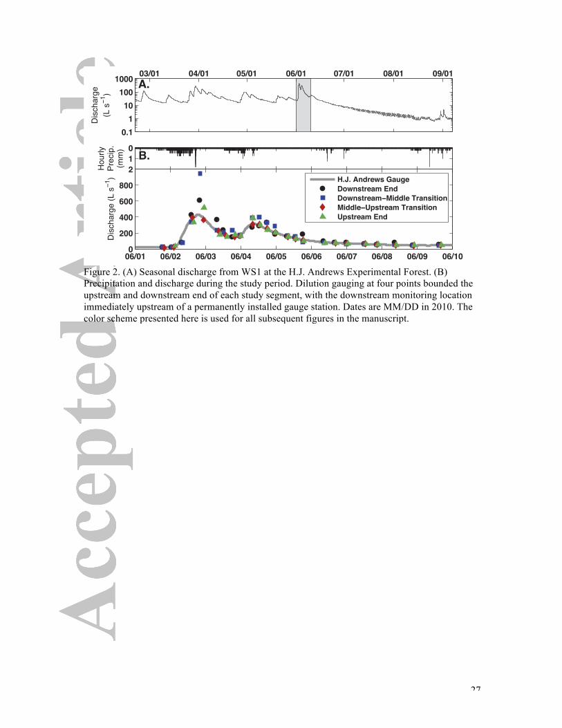
Figure 3. Water level observations are shown in the stream (blue lines extended horizontally from the observation point to the bank) and in monitoring wells and piezometers (black lines). Time segments depicted by each column are indicated by the shaded hydrograph at the top of each column. Darker colored lines represent conditions earlier in the time segment, and fade with equal temporal spacing to the end of the segment. Blue lines represent surface water elevations, and black lines potentiometric surface. Arrows indicate the direction of water level movement in each panel. The upstream and downstream segments are located on the north bank of the stream (left to right looking upstream; Figure 1C).

Rising Limb 1 Falling Limb 1 Rising Limb 2 Falling Limb 2

445

446

447El

evat

ion

(m)

0 5 10444

445

446

Elev

atio

n (m

)

X (m)0 5 10

X (m)0 5 10

X (m)0 5 10

X (m)

Upst

ream

Tra

nsec

tDo

wnst

ream

Tra

nsec

t

StreamStage

Potentiometric Surface

Ground Surface

Tim

e Tim

e

Tim

e

Tim

e

Tim

e

Tim

e

Tim

e Tim

e

Tim

e Tim

e

Tim

e Tim

e

Tim

e

Tim

e

Tim

e Tim

e

29

Figure 4. Left-hand panels show (A) net changes in flow, ΔQ, (B) tracer mass loss, (C) gross losses (QLOSS) and (D) gross gain (QGAIN) for each study reach. Boxplots and one-way ANOVA results summarize long-term storage (tracer mass that does not return to the stream channel within the window of detection) for each study reach. Long-term storage data and box-plots are associated with the left-hand Y-axes; discharge with the right-hand y-axes. ANOVA results

0

125

250

375

500

Disc

harg

e (L

s!1)

0

125

250

375

500

Disc

harg

e (L

s!1)

0

125

250

375

500

Disc

harg

e (L

s!1)

0

125

250

375

500

Disc

harg

e (L

s!1)

p=2.0E!01

p=4.1E!09

p=1.8E!02

p=1.4E!03

!400

!200

0

200

400

" Q

( L s!1

)

!60

!40

!20

0

20

Frac

tion

Mass

Los

s (%

)

!170

!125

!80

!35

10

Q LOSS

(L s!1

)

!10

45

100

155

210

Q GAIN

(L s!1

)

06/0

1

06/0

3

06/0

5

06/0

7

06/0

9

DischargeDownstream

MiddleUpstream

A.

B.

C.

D.

30

indicate the probability that at least one sample mean is drawn from a population with a different mean than the others. If tapered sections of the boxplots do not overlap the two medians are different at the 5% significance level. For example, in plot (C), the tapered sections for the upstream box does not overlap with the middle nor downstream reach boxes, so it is significantly different than both of those. Tapered sections for the middle and downstream boxes do overlap, so they are not significantly different. Dates are MM/DD in 2010.

31

Figure 5. Tracer window of detection (interpreted here at the time elapsed until 99% of the recovered mass is observed, t99) was inversely related to discharge in all three study reaches.

0 0.5 1 1.50

200

400

600

800

t99 (hr)

Q AVG (L

s!1)

UpstreamMiddleDownstream

32

Figure 6. Metrics of short-term storage for observed (left column) and normalized (right column) breakthrough curves. Left-hand panels show metrics of short-term storage for each study reach through time. Short-term storage data and box-plots are associated with the left-hand Y-axes; discharge with the right-hand y-axes. ANOVA results indicate the probability that at least one sample mean is drawn from a population with a different mean than the others. If tapered sections of the boxplots do not overlap, the two medians are different at the 5% significance level. For example, no tapered sections overlap in (J), indicating significant differences between all three reaches. Dates are MM/DD in 2010 on the X-axis.

0

125

250

375

500

Disc

harg

e (L

s!1)

0

125

250

375

500

Disc

harg

e (L

s!1)

0

125

250

375

500Di

scha

rge (

L s!1

)

1

10

100

1000

Disc

harg

e (L

s!1)

0

125

250

375

500

Disc

harg

e (L

s!1)

0

125

250

375

500

Disc

harg

e (L

s!1)

0

125

250

375

500

Disc

harg

e (L

s!1)

0

125

250

375

500

Disc

harg

e (L

s!1)

1

10

100

1000

Disc

harg

e (L

s!1)

0

125

250

375

500

Disc

harg

e (L

s!1)

Observed Breakthrough Curve Datap=8.8E!03

Normalized Breakthrough Curve Datap=1.0E!08

p=5.1E!03 p=1.0E!08

p=3.3E!01 p=1.9E!03

p=3.9E!01 p=1.2E!02

p=4.4E!12 p=3.9E!12

0

0.35

0.7

1.05

1.4t 99

(hr)

0

5

10

15

20

t 99,N

ORM

0

0.35

0.7

1.05

1.4

TSI (

hr)

0

5

10

15

20

TSI NO

RM

0

0.06

0.12

0.18

0.24

M 1 (hr)

1

1.3

1.6

1.9

2.2

M 1,NOR

M

0.0001

0.001

0.01

0.1

2(h

r )

0.1

1

10

100

! 2,NOR

M

0

2.5

5

7.5

10

"

06/0

1

06/0

3

06/0

5

06/0

7

06/0

9 0

2

4

6

8

" NORM

06/0

1

06/0

3

06/0

5

06/0

7

06/0

9

DischargeDownstreamMiddleUpstream

!2

A.

C.

E.

G.

I.

B.

D.

F.

H.

J.

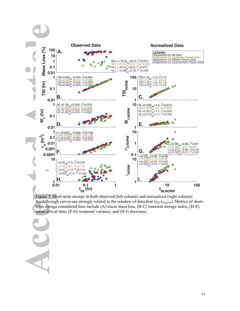
33

Figure 7. Short-term storage in both observed (left column) and normalized (right column) breakthrough curves are strongly related to the window of detection (t99, t99,norm). Metrics of short-term storage considered here include (A) tracer mass loss, (B-C) transient storage index, (D-E) mean arrival time, (F-G) temporal variance, and (H-I) skewness.

0.010.1

110

100Ma

ss L

oss (

%) Observed Data

M.L.=!10.3t99+23.3, r2=0.012M.L.= 27.5t99+25.0, r2=0.0.032M.L.= 25.4t99+20.8, r2=0.075M.L.=!0.48t99+0.03, r2=0.009

0.01

0.1

1

TSI (

hr)

TSI=0.96t99!0.020, r2=0.997TSI=0.98t99!0.019, r2=0.999TSI=0.95t99!0.018, r2=0.999TSI=0.86t99!0.004, r2=0.994

0.01

0.1

1

M 1 (hr)

M1=0.10t99+0.025, r2=0.576M1=0.08t99+0.017, r2=0.840M1=0.12t99+0.023, r2=0.873M1=0.25t99+0.003, r2=0.895

0.00010.001

0.010.1

1

2 (hr2 ) 2=0.024t99!0.004, r2=0.709

2=0.032t99!0.008, r2=0.746!2=0.019t99!0.003, r2=0.933!2=0.017t99!0.002, r2=0.916

0.01 0.1 11

10

"

t99 (hr)

"=3.3t99+1.5, r2=0.312"=1.8t99+3.1, r2=0.173"=3.0t99+1.2, r2=0.716"=0.85t99+1.4, r2=0.035

1

10

100

TSI NO

RM

TSI=1.0t99!1.0, r2=1.0TSI=1.0t99!1.0, r2=1.0TSI=1.0t99!1.0, r2=1.0TSI=1.0t99!1.0, r2=1.0

1

10

M 1,NOR

M

M1=0.036t99+1.2, r2=0.679M1=0.039t99+1.1, r2=0.694M1=0.061t99+1.1, r2=0.946M1=0.075t99+1.0, r2=0.706

0.1

1

10! 2,N

ORM

!2=0.28t99!0.86, r2=0.61!2=0.36t99!2.0, r2=0.57!2=0.31t99!0.96, r2=0.94!2=0.20t99!0.41, r2=0.95

10 1001

10

" NORM

t99,NORM

"=0.32t99+0.50, r2=0.80"=0.22t99+1.70, r2=0.60"=0.29t99+0.54, r2=0.83"=0.52t99!0.37, r2=0.84

0

1Normalized Data

LEGEND:Regression for all dataRegression for Upstream Reach dataRegression for Middle Reach dataRegression for Downstream Reach data

A.

C.

E.

G.

I.

B.

D.

F.

H.

!

!!

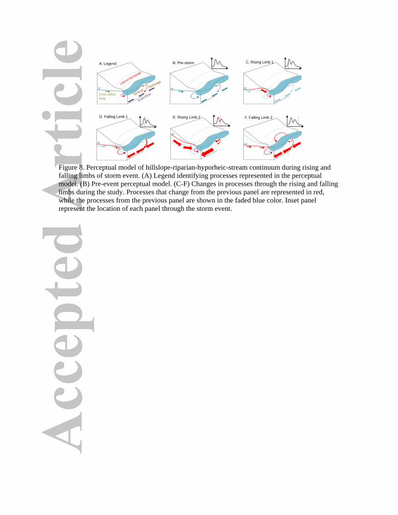
Cross‐valley��Flow�

A. Legend B. Pre-storm C. Rising Limb 1

E. Rising Limb 2 D. Falling Limb 1 F. Falling Limb 2

Figure 8. Perceptual model of hillslope-riparian-hyporheic-stream continuum during rising and falling limbs of storm event. (A) Legend identifying processes represented in the perceptual model. (B) Pre-event perceptual model. (C-F) Changes in processes through the rising and falling limbs during the study. Processes that change from the previous panel are represented in red, while the processes from the previous panel are shown in the faded blue color. Inset panel represent the location of each panel through the storm event.

Auxiliary material submission for Paper 2012WR013185 How does rapidly changing discharge during storm events affect transient storage and channel water balance in a headwater mountain stream? Adam S. Ward Department of Earth and Environmental Sciences, The University of Iowa, Iowa City, IA 52242. USA. Michael N. Gooseff Department of Civil and Environmental Engineering, Colorado State University, Fort Collins, CO 80523. USA. Thomas J. Voltz Division of Water Sciences, Faculty of Civil Engineering & Architecture, University of Applied Sciences Dresden, 01069 Dresden, Germany. Michael Fitzgerald National Ecological Observatory Network, Boulder, CO 80301. USA. Kamini Singha Hydrologic Science and Engineering Program, Colorado School of Mines, Golden, CO 80401. USA. Jay P. Zarnetzke Department of Geological Sciences, Michigan State University, East Lansing, MI 48824. USA. Introduction This set of auxiliary material contains the observed and normalized in-stream solute tracer time series analyzed in the associated manuscript (Figure S1). A description of supplemental files is provided below. 1. 2012WR013185-fs01.pdf Observed solute tracer breakthrough curves (left column) and normalized solute breakthrough curves (right column). For the left column, time is elapsed from the peak at the upstream monitoring station and concentration is the change from pre-injection conditions. For the right column, time is normalized by the advective travel time in the reach, and concentration is normalized by the zeroth moment. Curve color indicates relative time in the study, with a black curve representing the first slug injection at each location, and the lightest color representing the latest slug injection.