Embed Size (px)
Citation preview
HAL Id: halshs-00534754https://halshs.archives-ouvertes.fr/halshs-00534754
Submitted on 10 Nov 2010
HAL is a multi-disciplinary open accessarchive for the deposit and dissemination of sci-entific research documents, whether they are pub-lished or not. The documents may come fromteaching and research institutions in France orabroad, or from public or private research centers.
L’archive ouverte pluridisciplinaire HAL, estdestinée au dépôt et à la diffusion de documentsscientifiques de niveau recherche, publiés ou non,émanant des établissements d’enseignement et derecherche français ou étrangers, des laboratoirespublics ou privés.
How does investor sentiment affect stock market crises?Evidence from panel dataM. Zouaoui, G. Nouyrigat, F. Beer
To cite this version:M. Zouaoui, G. Nouyrigat, F. Beer. How does investor sentiment affect stock market crises? Evidencefrom panel data. Cahier de recherche n° 2010-08 E2. 2010. <halshs-00534754>

How does investor sentiment affect stock market crises?
Evidence from panel data
Mohamed ZOUAOUI
Geneviève NOUYRIGAT
Francisca BEER
CAHIER DE RECHERCHE n°2010-01 E1
Unité Mixte de Recherche CNRS / Université Pierre Mendès France Grenoble 2 150 rue de la Chimie – BP 47 – 38040 GRENOBLE cedex 9
Tél. : 04 76 63 53 81 Fax : 04 76 54 60 68
-1-
How does investor sentiment affect stock market crises? Evidence from panel data
Mohamed ZOUAOUI University of Franche-Comté
LEG-UMR 5118 [email protected]
Tel: 0033 381 666 642
Geneviève NOUYRIGAT University of Grenoble CERAG-UMR 5820
[email protected] Tel: 0033 475 418 844
Francisca BEER
California State University of San Bernardino [email protected]
Tel: 001 909 880 5709
April 4, 2010 Abstract
We test the impact of investor sentiment on a panel of international stock markets. Specifically, we examine the influence of investor sentiment on the probability of stock market crises. We find that investor sentiment increases the probability of occurrence of stock market crises within a one-year horizon. The impact of investor sentiment on stock markets is more pronounced in countries that are culturally more prone to herd-like behavior and overreaction or in countries with low institutional involvement. Results also suggest that investors’ sentiment is not a reliable predictor of stock market reversal points.
JEL Classification : G12, G14, G15. Keywords: Investor sentiment, stock market crises, reversal points.

-2-
Introduction
Financial professionals are well aware of the impact of investors’ psychology on financial
markets. The influence of investors’ mood on market movements is regularly discussed in
financial periodicals, on the radio and on television. As noted by Daniel Kahneman in a
speech entitled "Psychology and Market" at Northwestern University in 2000: "If you listen to
financial analysts on the radio or on TV, you quickly learn that the market has a psychology.
Indeed, it has character. It has thoughts, beliefs, moods, and sometimes stormy emotions."
Traditional financial models have difficulty explaining financial crises. The crash of October
1987, for instance, remains enigmatic for researchers. During the crash, stock prices drop an
average of 22.6%, a decrease much larger than what can be explained by changes in economic
variables (Black, 1988; Fama, 1989; Shiller, 1989; Seyhun, 1990; Siegel, 1992).The view
about the market "personality", the market behavioral approach recognizes that investors are
not "rational" but "normal" and that systematic biases in their beliefs induce them to trade on
non-fundamental information, called "sentiment". Recently, investor sentiment has become
the focus of studies on asset pricing.
Several theoretical studies offer models establishing the relationship between investors’
sentiment and assets prices (Black, 1986; De Long, Shleifer, Summers and Waldmann, 1990;
Barberis, Shleifer and Vishny, 1998; Daniel, Hirshleifer and Subrahmanyam, 2001). Two
categories of investors characterize these models: informed traders rationally anticipating
asset value and uninformed noise traders who experienced waves of irrational sentiment.
Rational traders, who are sentiment free, correctly evaluate assets. Uninformed noise traders’
overly optimistic or pessimistic expectations induce strong and persistent mispricing. In these
models, informed traders and noise traders compete. Informed traders, the unemotional
investors, who force capital market prices to equal the rational present value of expected
future cash flows, face non-trivial transactions and implementation costs as well as the
-3-
stochastic noise trader sentiment. These elements prevents informed traders from taking fully
offsetting positions to correct mispricing induced by noise traders. Hence, to the extent that
sentiment influences valuation, taking a position opposite to prevailing market sentiment can
be both expensive and risky. Mispricing arises out of the combination of two factors: a change
in sentiment on the part of the noise traders, and a limit to arbitrage.
Several empirical studies attempt to measure investor sentiment (Lee, Shleifer and Thaler,
1991; Neal and Wheatley, 1998; Brown and Cliff, 2004). These studies identified direct and
indirect sentiment measures. Direct sentiment measures are derived from surveys while
indirect measures relied on objective variables that correlate with investor sentiment.
Numerous significant publications focus on the impact of sentiment on future stock returns
(Solt and Statman, 1998; Brown and Cliff, 2005; Baker and Wurgler, 2006). Finding shows
that individual investors are easily swayed by sentiment. Sentiment indicators increases the
traditional model explanatory power for stocks that are highly subjective and difficult to
arbitrage, e.g small stocks, value stocks, stocks with low prices and stocks with low
institutional ownership.
Despite the number of published works on the issue of investor sentiment, several avenues
of research remain unexplored. In particular, the empirical question of a relationship between
sentiment and stock market crises remains under researched and unresolved. Fluctuations in
investor sentiment are often mentioned as a factor that could explain the financial crises but
rarely analysed (White, 1990; De Long and Shleifer, 1991; Shiller, 2000). Most previous
studies test the ability of sentiment indicators to predict stock prices in aggregate or in period
of normal market conditions. Few studies have attempted to directly link sentiment indicators
to market crises. Only two studies were identified and those were limited to the U.S. stock
market crash of 1987 (Siegel 1992 and Baur, Quintero and Stevens, 1996).
-4-
Our goal, therefore, is to study the ability of sentiment indicators to predict international
stock market crises. To achieve our objective, we built a "leading indicator" of crises using
data from 16 countries. By means of a logit model, we related our qualitative crises indicator
to a set of quantitative macro-economic variables and the indicator of sentiment. Specifically,
we tested whether consumer confidence - as a direct proxy for individual investor sentiment-
influenced the probability of stock market crises in 16 countries. Results confirmed the
significant impact of investors’ sentiment on financial crises. The impact of sentiment is more
pronounced for countries that are culturally more prone to herd-like behavior and overreaction
and countries with low institutional development.
Our study diverges from previous research in several ways. First, we use investors’
sentiment as an indicator of financial crises. A better grasp of stock market crises should
deepen our understanding of the dynamic process of stock price adjustments to intrinsic value.
Second, our sample of different countries allows comparisons with U.S. data. Furthermore,
the use of panel data is known to generate more accurate predictions for individual outcomes
by pooling the data (Ang and Bekaert, 2007). Third, taking an international perspective allows
us to analyse the cross-country variation in the sentiment-return relationship. A cross-country
study can provide evidence on how cultural differences as well as institutional differences
affect the sentiment-return relation. Finally, focusing on stock market crises allows us to
examine the concept of price reversal, another under researched phenomenon.
The remainder of this article is organized as follows. The second section is devoted to a
summary of the literature. The third section presents the methodology and variables used to
explain the probability of a stock market crisis. The fourth section analyzes the empirical
results obtained. The fifth section investigates cross-country results. In the sixth section,
results from the test conducted on price reversal are presented. The seventh section concludes
the study.

-5-
2. Literature Review
The relationship between the variables sentiment and stock returns is at odds with classic
finance theory which states that stock prices mirror the discounted value of expected cash-
flows and that irrationalities among market participants are removed by arbitrageurs.
Behavioral finance, on the other hand, suggests that optimistic and/or pessimistic investors’
expectations affect asset prices. Baker and Wurgler (2006) pointed out that sentiment-based
mispricing is based on an uninformed demand of some investors, the noise traders, and a limit
to arbitrage. Since it is unknown how long buying or selling pressures from overly optimistic
or pessimistic noise traders will persist, mispricing can be persistent. However, every
mispricing must eventually be corrected so one should observe that high levels of investor
optimism are followed by low returns and vice versa.
Validation for behavioral finance started with studies examining the correlation between
macro-economic variables and stock prices. The process by which security prices adjust to the
release of new information has also been studied extensively. Results of these studies show
that stock prices reflect more than fundamental variables. As early as 1971, Niederhoffer
highlights the weak stock market reaction to events considered important (Election, War,
Change of foreign leadership…, etc,) while very strong asset price variations remain difficult
to explain. More recently, Cutler, Poterba and Summers (1991) examined stock price changes
in relation to the arrival of information about macro-economic performance. They established
that macro-economic variables explained approximately a third of the variance in stock
returns. They also showed that information, such as news about wars, the presidency, or
significant changes in financial policies explain some but not all of the variance in stock
returns. These findings are similar to those reported by Shiller (2000) who established that
volatility of market prices are well above what is predicted by changes in economic
indicators.
-6-
Stock price volatility during crashes defies the explanatory power of the traditional
financial models. The conventional models, in which unemotional investors force capital
market prices to equal the rational present value of expected future cash flows, have
considerable difficulty explaining stock price volatility. Researchers in finance have therefore
been working to supplement these traditional models. Shiller (1987) surveyed both individual
and institutional investors inquiring about their behavior during the 1987 crash. He showed
that most investors interpreted the crash as the outcome of other investors’ psychology rather
than fundamental financial variables such as earnings or interest rates. Siegel (1992)
confirmed that changes in corporate profits and interest rates were unable to explain the rise
and subsequent collapse of stock prices in 1987. He suggested that a shift in investor
sentiment was a factor in the stock market’s deep decline1. During his speech on December 5,
1996 at the American Enterprise Institute, Greenspan delivered his memorable line that
“....irrational exuberance has unduly escalated asset values...”. Greenspan’s warning,
unfortunately, did not prevent the swelling and bursting of the tech bubble in 2000.
The events of 1987 and 2000 have led several well renowned financial economists to
distance themselves from the traditional finance theory (Black, 1986; Shiller 1989; Thaler,
1999; Rubinstein, 2001; Shefrin, 2005). Most financial economists recognized that the market
has mood swings and considered behavioral finance as an alternative. The link between asset
valuation and investor sentiment became the subject of considerable deliberation among
financial economists. A vast number of empirical investigations with different measures of
investor sentiment have been conducted. While theoretical models have incorporated the
existence of noise traders into equilibrium asset pricing early, empirical evidence on the
correct proxy for sentiment or on the significance of investor sentiment does not provide clear
findings.
1 Contrary to this finding, Baur, Quintero and Stevens (1996) reported that during the periods that surrounded the crash, only changes in fundamentals have a statistically significant impact on the movement of stock prices.
-7-
Neal and Wheatley (1998) examined the forecast power of three popular measures of
individual investor sentiment: the level of discounts on closed-end funds, the ratio of odd-lot
sales to purchases and the net mutual fund redemptions. They found that net fund redemptions
predict the size premium and the difference between small and large firm returns. They also
reported a positive relationship between discounts and small firm’s expected returns but no
relationship between discount and large firm’s expected returns. These results are consistent
with the investor sentiment hypothesis that small firms stocks are held primarily by small
investors. Brown and Cliff (2004) scrutinize various direct and indirect sentiment indicators.
They report that direct (surveys) and indirect measures of sentiment are correlated. Although
indicators of sentiment strongly correlated with contemporaneous market returns, they show
that sentiment has little predictive power for near-term future stock returns. Qiu and Welch
(2006) reported that surveys measuring investors’ sentiment are related to other popular
measures of investors’ sentiment and to recent stock market returns. They also showed that
although indirect measures circumvent the lack of sample size and statistical
representativeness of the direct measurements, the theoretical link to investor sentiment is
weaker than with the direct indicators.
Other indirect indicators using statistical series from futures trading activities can also be
found in the literature. Simon and Wiggins (2001) measured sentiment using the put-call ratio
and found that the sentiment indicators are statistically and economically useful contrarian
indicators in the S&P 500 futures market. Schmitz, Glaser, and Weber (2005) identified
warrant trades as an effective measure of sentiment. Lee and Song (2003) measured noise
investors’ sentiment with the equity put-call ratio and the market volatility (VIX) index.
Their findings provided insights into the relationship between trading volume and volatility
by considering the changing sentiments of different traders. Baker and Wurgler (2006)
constructed an index of investor sentiment as the first principal component of six indirect

-8-
investor measures suggested in the literature (trading volume as measured by NYSE turnover;
the dividend premium; the closed-end fund discount; the number and first-day returns on
IPOs; the equity share in new issue). They found that the sentiment effects are stronger among
stocks whose valuations are highly subjective and difficult to arbitrage.
Much work has been aimed at studying the impact of direct measures on the stock returns.
However, the results of these investigations have also been mixes. Solt and Statman (1988)
and Clarke and Statman (1998) find that the sentiment indicator published by Investors
Intelligence is useless as an indicator of future stock price changes. Fisher and Statman (2000)
studied the sentiments of three groups of investors: small investors, newsletter writers, and
Wall Street strategists, and found that the sentiments of both small investors and Wall Street
strategists were reliable contrary indicators for future S&P 500 stock returns, but no
statistically significant relation between the sentiment of newsletter writers and stock returns
was uncovered. Using survey data on investor sentiment, Brown and Cliff (2005) provided
evidence that sentiment affects asset valuation. The authors show that excessive optimism
leads to periods of market overvaluation and high current sentiment is followed by low
cumulative long-run return.
Other studies focusing on indexes of consumer confidence analyzed the impact of
sentiment on the stock market. Otoo (1999) reported a strong contemporaneous relationship
between changes in the consumer confidence index and the stock returns. Examining the
causal relationship among the variables, she stated that returns Granger-cause consumer
confidence at very short horizons but not vice versa. Fisher and Statman (2003) found
statistically significant relationships between some components of consumer confidence and
subsequent NASDAQ and small cap returns. Charoenrook (2006) examined whether
sentiment, as measured by yearly change in the University of Michigan Consumer Sentiment
Index, has affected stock returns. The author found that changes in the index reliably
-9-
predicted excess stock market returns. Lemmon and Portniaguina (2006) also reported
evidence that investors appear to overvalue small stocks relative to large stocks during
periods when consumer confidence is high and, vice versa. Moreover, Schmeling (2009)
examined whether consumer confidence affects expected stock returns in 18 industrialized
countries. In line with recent evidence for the U.S, he found that sentiment negatively
forecasts aggregate stock market returns on average across countries. This relation also holds
for returns of value stocks, growth stocks, small stocks, and for different forecasting horizons.
Similarly, Baker, Wurgler and Yuan (2009) constructed indexes of investor sentiment for six
major stock markets and decomposed them into one global and six local indices. They
determined that sentiment, both global and local, is a statistically and economically significant
contrarian predictor of market returns, particularly for highly subjective and difficult to
arbitrage stocks. This extends prior US evidence to international markets.
The prior literature review highlights the lack of consensus about the best measure of
sentiment or on whether sentiment in fact affects stock prices. While existing studies test the
impact of sentiment on individual stocks and portfolios of stocks whose valuations are highly
subjective and difficult to arbitrage, this paper takes a different approach. We propose to test
the impact of investor sentiment on international capital markets by studying its ability to
predict stock market crises. A priori, stock market crises should be preceded by periods of
rising investor euphoria. Therefore, we expect that periods characterized by excessive
investors’ optimism are followed by stock market crises.
3. The stock market crises and the role of investor sentiment
As mentioned above, our goal is to test the ability of investor sentiment to predict
international stock market crises. The study includes 15 European countries and the United
States. Data includes monthly observations for the period between April 1995 and June 2009.
Economic data availability dictated the beginning time period for most countries. As

-10-
discussed below, our study includes financial and macro-economic variables and survey
results. The list of the countries and the data sources used are presented respectively in
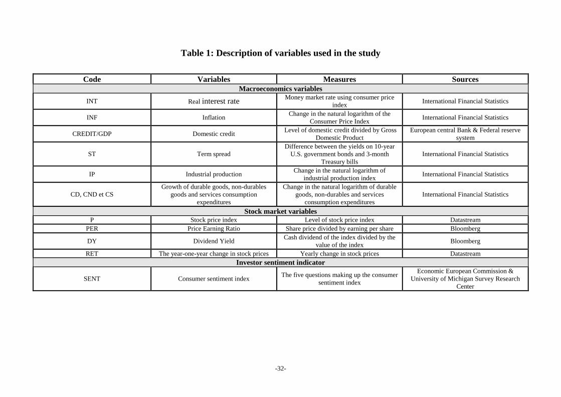
appendix 1 and table 1.
[INSERT TABLE 1] 3.1. Identification of stock market crises Most studies define equity crises as an abrupt and rapid drop in the overall market index.
The change of the index can be the predecessor of larger decreases, higher dispersions of
probable losses and/or more uncertainty about the return of firms. The first step of our study
consists of identifying the financial crises that have occurred during the period considered in
the regions studied. To achieve this goal, we use the methodology proposed by Patel and
Sarkar (1998) which is, according to these authors, widely used by practitioners.
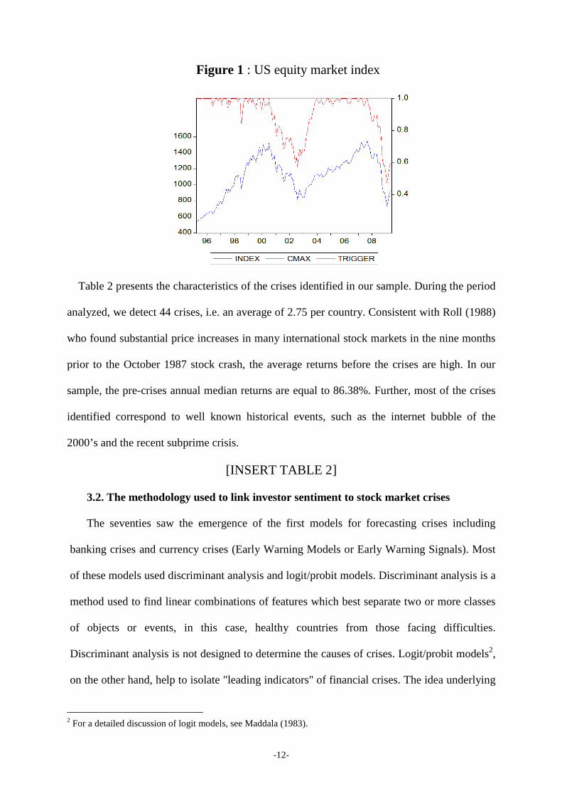
In their study, Patel and Sarkar (1998) designed a crises indicator called CMAX. The
CMAX compares the current value of an index with its maximum value over the previous T
periods, usually 1 to 2 years. The CMAX ratio is calculated by dividing the current price by
the maximum price over the previous two year period.
)...,max( ,24,
,,
titi
titi PP
PCMAX
−
=
Where Pit is the stock market index at time t for country i. The rolling maximum in the
denominator was defined over a relatively short period (24 months) to avoid losing too many
data points.
Boucher (2004) describes the CMAX as an indicator of the decline in volatility. This
indicator equals 1 if prices rise over the period considered, indicating a bullish market. The
more prices fall, the closer the CMAX gets to 0. A crisis is detected whenever CMAX
exceeds a threshold set at the mean of CMAX minus two standard deviations. To avoid

-11-
counting the same crisis more than once, a crisis is automatically eliminated if detected twice
over a twelve month period.
The stock market crises indicator for country i at time t, Ci,t, is defined as follow:
iiti CMAXC σ 2CMAX if 1 ti,, −<= otherwise ,0, =tiC
Given the indicator structure, share price decreases are already well in progress when a
crisis is identified, i.e. Ci,t uncovers abnormal drops in prices rather than the market turning
point. This indicator only identifies as crises those events that eliminate the previous two
years of gains.
Similarly to Patel and Sarkar (1998), we define the following concepts : (i) the beginning
of a crises as the month when the index reaches its historical maximum over the 2-year
window prior to the month when the crash is triggered, (ii) the beginning of the crash
corresponds to the month when the CMAX intersects with a threshold, (iii) the date of trough
is the month when the price index reaches its minimum, (iv) the date of recovery is the first
month after the crash when the index reaches the pre-crash maximum, (v) the magnitude of
the crises is the difference between the value of the index at its maximum and at its minimum,
(vi) the length of the trough is the number of months between the date of the beginning of the
crises and the date of the trough, and (vii) the length of the recovery period is the number of
months for the index to return to the maximum.
Figure 1 illustrates these concepts on the US stock market. As shown, three crises are
identified during the period 1995-2009. The first crash occurred in July 2001 and reached a
trough eleven months later in June 2002. It was characterized by a decrease of 40% in the
S&P500 and the crisis ended 81 months later, in April 2007. The second crash took place in
August 2002. It took 52 months for the market to regain the 43% loss during the crisis. The
third crash is identified in June 2008 and the magnitude of the crises is 52.55 %.
-12-
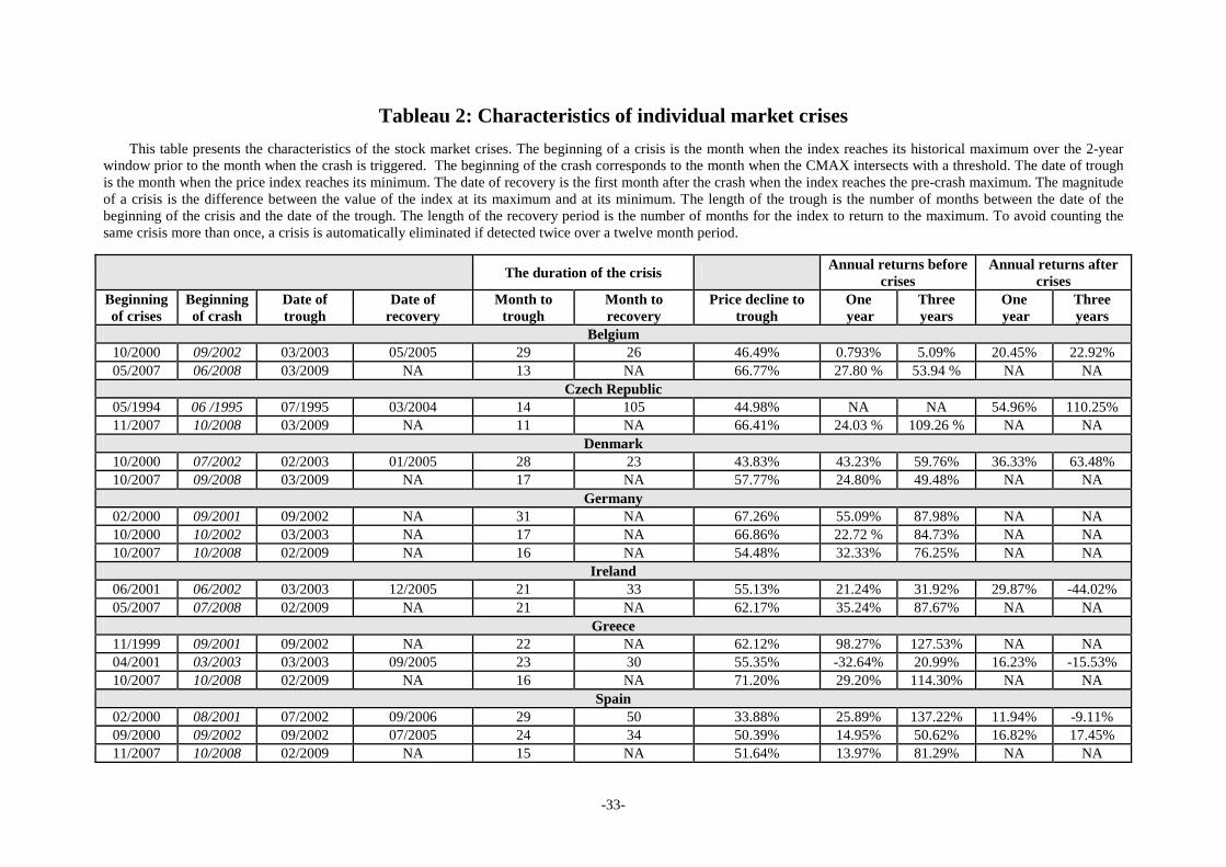
Table 2 presents the characteristics of the crises identified in our sample. During the period
analyzed, we detect 44 crises, i.e. an average of 2.75 per country. Consistent with Roll (1988)
who found substantial price increases in many international stock markets in the nine months
prior to the October 1987 stock crash, the average returns before the crises are high. In our
sample, the pre-crises annual median returns are equal to 86.38%. Further, most of the crises
identified correspond to well known historical events, such as the internet bubble of the
2000’s and the recent subprime crisis.
[INSERT TABLE 2] 3.2. The methodology used to link investor sentiment to stock market crises The seventies saw the emergence of the first models for forecasting crises including
banking crises and currency crises (Early Warning Models or Early Warning Signals). Most
of these models used discriminant analysis and logit/probit models. Discriminant analysis is a
method used to find linear combinations of features which best separate two or more classes
of objects or events, in this case, healthy countries from those facing difficulties.
Discriminant analysis is not designed to determine the causes of crises. Logit/probit models2,
on the other hand, help to isolate "leading indicators" of financial crises. The idea underlying
2 For a detailed discussion of logit models, see Maddala (1983).
Figure 1 : US equity market index
-13-
these models is to identify economic variables having a specific behavior before the onset of
the crises and to estimate the probability of occurrence of these crises during a specific period
(usually one or two years), taking into account the information these variables included
(Frankel et Rose, 1996; Demirguc-Kunt et Detragiache, 2000; Bussiere et Fratzscher, 2006;
Lau et Yan, 2005). Our approach, outlined below, is inspired by the logit/probit models.
� The dependent variable The logit approach has the advantage of providing a framework for statistically
measuring the magnitude and significance of the effects of various explanatory variables on
the onset of a financial crisis. It explains the occurrence or the non-occurrence of a crisis with
a binary variable and explanatory variables found in the real sector of the economy, i.e.
financial variables, external sector and fiscal variables.
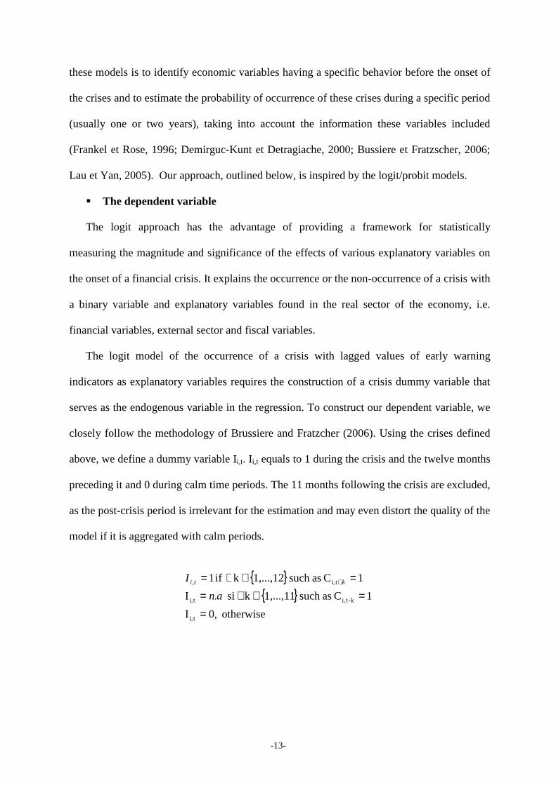
The logit model of the occurrence of a crisis with lagged values of early warning
indicators as explanatory variables requires the construction of a crisis dummy variable that
serves as the endogenous variable in the regression. To construct our dependent variable, we
closely follow the methodology of Brussiere and Fratzcher (2006). Using the crises defined
above, we define a dummy variable Ii,t. Ii,t equals to 1 during the crisis and the twelve months
preceding it and 0 during calm time periods. The 11 months following the crisis are excluded,
as the post-crisis period is irrelevant for the estimation and may even distort the quality of the
model if it is aggregated with calm periods.
{ }
{ }otherwise ,0I
1C assuch 1,...,11k si .I
1C assuch 1,...,12k if 1
ti,
k-ti,ti,
ti,,
==∈∃=
=∈∃= +
an
I kti

-14-
� The independent variables
The following sub-sections present the variables proposed to explain the crises detected
in the sample. The first sub-section introduces “traditional” variables. The second sub-section
focuses on the variable sentiment.
• The traditional variables Contrary to banking and currencies crises where studies are abundant, very few studies
have been published about the variables explaining the stock market crises. For the period
1929 – 2000, the literature indentified two groups of variables3.
The first group of explanatory variables reflects the price acceleration and the divergence
between asset prices and their intrinsic value. The variables are the year-on-year change in
stock prices (RET) and the price earnings ratios (PER).
The RET is a good substitute for price acceleration and decline. Indeed, the returns tend to
decline gradually before the onset of the crisis. The PER is widely used to express a firm's
market valuation relative to its fundamental value. Campbell and Shiller (2001) showed that
when stock market valuation ratios are at extreme levels by historical standards, some weight
should be given to the mean-reversion theory that prices will fall in the future to bring the
ratios back to more normal historical levels. Indeed, If we accept the premise for the moment
that valuation ratios will continue to fluctuate within their historical ranges in the future, and
neither move permanently outside nor get stuck at one extreme of their historical ranges, then
when a valuation ratio is at an extreme level either the numerator or the denominator of the
ratio must move in a direction that restores the ratio to a more normal level.
The second group of variables includes monetary aggregates and an indicator of financial
instability. In this category, we retain inflation rate (INF), real interest rate (INT) and ratio
domestic credit/GDP (CREDIT).
3 These variables are similar to those proposed by Boucher (2004) and Goudret and Gex (2008).
-15-
Stock prices are negatively correlated to inflation and financial crises are characterized by
high volatility of inflation (Nelson, 1976; Fama et Schwert, 1977; Blanchard, 1993). For
example, Fama and Schwert (1977) established that most stock markets have the tendency to
perform poorly when inflation is high. Using US data since 1789, Bordo and Wheelock
(1998) showed that most financial crises occurred during periods with high variation in
inflation. The interest rates are also often cited as a good indicator of financial crises. Interest
rates tend to decline significantly before the collapse of the stock markets. Finally, Domestic
credit, another independent variable, is used to capture financial instability often visible
before financial crises. As documented in Corsetti, Pesenti and Roubini (1998), Goldstein
(1998) and Kamin (1999), when domestic credit grows at a fastest rate than GDP, this can
lead to excessive risk-taking from investors with large losses on loans in the future. With
rapid growth of lending, banking institutions might not be able to add the necessary
managerial capital (well-trained loan officers, risk-assessment systems, etc.) fast enough to
enable these institutions to screen and monitor these new loans appropriately. The outcome of
the lending boom leads to the deterioration in bank balance sheets, leading economies into
financial crises.
• The behavioral variable A universally accepted measure of investor sentiment has not yet been identified. The
financial literature proposes two categories of proxies for investor sentiment, direct and
indirect indicators. Direct sentiment measures are based on polling market participants
through surveys. Indirect measures are made up of a time series of macro-economic and
financial variables, used to proxy the unobserved sentiment factor4.
For this study, we favored the consumer confidence index5. This variable seizes some of
the crises aspects not already contained in macro-economic indicators. The use of the
4 See, for instance, Brown and Cliff (2004) for a detailed discussion of sentiment measures. 5 Details of consumer confidence survey are given in Appendix 2.

-16-
consumer confidence index appeared logical. First, data on the consumer confidence index is
available for the majority of developed countries since the mid-80s. Second, because most
countries use similar surveys to gather data, comparisons across countries are possible6.
Notice that we are not alone; among the various direct indicators, the consumer
confidence index seems to be the preferred indicator of the majority of researchers. Otoo
(1999), Fisher and Statman (2003), Qiu and Welch (2006) and Lemmon and Portniaguina
(2006) presented several additional arguments in support of this variable:
• Although consumers polled for the University of Michigan Consumer Confidence Index
are not asked directly for their views on security prices, changes in the Consumer
Confidence Index correlate very highly with changes in stock prices.
• Participation of individual households in financial markets has increased substantially
over recent years suggesting that measures of consumer confidence may be a useful
barometer of how individual investors feel about the economy and the financial markets
• Researchers utilize longitudinal data which allows for more robust and significant studies.
Direct measures of sentiment derived from surveys circumvent some of the drawbacks of
indirect measures7.
• Because the consumer confidence index captures individual beliefs, it reflects the
philosophy of behavioral finance; including the opinions of imperfect people who have
social, cognitive, and emotional biases (Shleifer, 2000).
Finally, as many researchers8 emphasize that the direct indicator of sentiment reflects an
economic component and a psychological aspect, we decompose the consumer confidence
index into a component related to the business cycle, i.e. macroeconomic “fundamentals” and
6 The European questionnaires have been harmonized since the mid-80s. Michigan consumer confidence survey covers 5 years. The European survey covers 1 year and has an average number of participants of 3000 respondents. 7 Because indirect measures are made up of time series of macro-economic and financial variables, they may not exclusively represent investors’ sentiment. 8 See Brown and Cliff (2005), Lemmon and Portniaguina (2006), Kumar and Lee (2006) and Baker and Wurgler (2006).

-17-
a residual component that we interpret as a purer measure of “sentiment” (SENT⊥).
Specifically, we treat the residual from the following regression as our measure of sentiment
unwarranted by fundamentals9.
,1
,, ti
J
j
jtij FUNDSENT
tiεβα ++= ∑
=
⊥
The variables that capture the component related to the business cycle, i.e.
macroeconomic “fundamentals” (FUND) are: (i) the changes of the industrial production (IP),
(ii) the growth in consumption of durables (CD), non-durables (CND) and services (CS), (iii)
the spread defined as the difference in yield between the 10-year and 3-month government
bonds (ST) and (iv) the dividend yield measured as the dividend divided by the market
capitalization (DY). We believe that these variables are as comprehensive as those commonly
used in the literature. This procedure reduces the likelihood that variation in sentiment is
related to systematic macroeconomic risks. The sentiment measure is orthogonalized with
respect to several contemporaneous variables.
� The model used The dependent variable Ii,t is explained by the macro-economic indicators and the variable
sentiment via a logit model, i.e. we explained our crises indicator (Ii,t) with a set of
quantitative macro-economic variables and the indicator of sentiment. In seeking to estimate
the probability that the variable Ii,t is equal to 1, we estimate the probability of a crisis within a
1 year window. In other terms, the model attempts to predict whether a crisis will occur
during the coming 12 months.
Specially, we successively estimate three different logit models. Model 1 includes only
macro-economic variables. Model 2 focuses on sentiment. Model 3 combines macro-
economic and sentiment variables10.
9 Due to lack of space, we are not reporting all the regression results. Detailed results are available upon request. 10 The explanatory variables have been standardized to insure comparability for all countries.
-18-
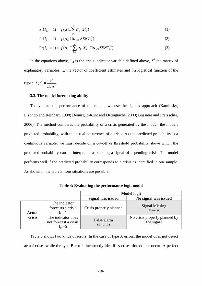
) ()1Pr(1
,, ∑=
+==n
k
ktikti XfI αα (1)
)()1Pr( , 10,⊥
++== tinti SENTfI αα (2)
) ()1Pr(1
,1,'
, ∑=
⊥+++==
n
ktin
ktikti SENTXfI ααα (3)
In the equations above, Ii,t is the crisis indicator variable defined above, Xk the matrix of
explanatory variables, αk the vector of coefficient estimates and f a logistical function of the
type : z
z
e
ezf
+=
1)( .
3.3. The model forecasting ability
To evaluate the performance of the model, we use the signals approach (Kaminsky,
Lizondo and Reinhart, 1998; Demirguc-Kunt and Detragiache, 2000; Bussiere and Fratzscher,
2006). The method compares the probability of a crisis generated by the model, the models
predicted probability, with the actual occurrence of a crisis. As the predicted probability is a
continuous variable, we must decide on a cut-off or threshold probability above which the
predicted probability can be interpreted as sending a signal of a pending crisis. The model
performs well if the predicted probability corresponds to a crisis as identified in our sample.
As shown in the table 3, four situations are possible:
Table 3: Evaluating the performance logit model
Model logit
Signal was issued No signal was issued The indicator
forecasts a crisis Iit =1
Crisis properly planned Signal Missing (Error A)
Actual crisis The indicator does
not forecast a crisis Iit =0
False alarm (Error B)
No crisis properly planned by the signal
Table 3 shows two kinds of errors. In the case of type A errors, the model does not detect
actual crises while the type B errors incorrectly identifies crises that do not occur. A perfect
-19-
indicator would only produce observations that belong to the north-west (NW) and south-east
(SE) cells of this matrix, minimizing the type A and type B errors.
The performance of logit model depends largely on these two types of errors. The main
question is the optimal threshold level. The lower the threshold, the more signals the model
will send with the drawback of having numerous false signals. By contrast, raising the
threshold will reduce the number of false signals at the expense of an increase in the number
of missed crises signals. Notice, however that the costs associated with the two types of errors
are not the same. Type A errors, missing a crisis that ended up materializing, are larger than
type B errors consisting of incorrectly anticipating a crisis that will not occur. As suggested
by Berg and Patillo (1998), Boucher (2004) and Coudert and Gex (2008), we decided to
present the results for alert thresholds set at 25% and 50%.
4. Regression results
Our goal is to estimate the incremental predictive power of the sentiment variable
compared to other variables habitually used in the literature. The findings are presented in
three parts. Part 1 shows the results of a model including the fundamental economic and
financial variables. Part 2 focuses on the sentiment variable. Part 3 combines economic,
financial and sentiment indicators. Table 4 presents the results.
[INSERT TABLE 4]
4.1. The predictive power of the traditional variables
With the exception of the INF variable, all macro-economic variables included in Model 1
are significant and display the expected sign. The model is performing well, the maximum
likelihood confirms the quality of the overall fit of the model and the hypothesis of joint
nullity of all the regression coefficients except the constant can be rejected.
These findings add credibility to PER, RET, INT and CREDIT as predictors of financial
crises. Bubbles are often characterized by an unsustainable increase in asset prices.
-20-
Traditionally, the PER is used to give an idea of what the market is willing to pay for the
company’s earnings. A stock with a high PER is often interpreted as an overpriced stock
while a stock with low PER may indicate a “vote of no confidence.” Our study shows that an
increase in the PER is positively correlated with the probability of a financial crisis. This
result supports the mean-reversion theory that when prices are high they will fall, bringing the
PER back to normal historical levels.
The variable INT negatively impacts the probability of a financial crisis. This result
explains why monetary authorities cut rates to stabilize the economy and limit the adverse
consequences of bursting bubbles. The sign is also negative for retuns (RET), which already
tend to decline at the onset of the crisis. As far as the variable CREDIT is concerned, a
positive and significant coefficient supports previously reported studies that financial
aggregates, such as domestic credit, are early indicators of financial crises. Rapid credit
growth has been associated with macroeconomic and financial crises, originating from
macroeconomic imbalances and banking sector distress. This is why policymakers face the
dilemma of how to minimize the risks of financial crisis while still allowing bank lending to
contribute to higher growth and efficiency.
Contrary to our expectations, the variable INF is negatively correlated to the probability of
a financial crisis. A significant negative coefficient is intuitively difficult to comprehend as it
implies that policymakers' commitment to price stability increases the probability of a crisis.
A negative correlation, can however, be explained by the “paradox of credibility”.
Goodfriend (2001) and Borio and Lowe (2002) showed that when inflation is under control,
tensions of productivity cannot be detected by inflation numbers but rather by instability in
the financial sector11. The idea has been shared by the BIS economists, who have been
11 The bursting of the technology bubble in the beginning of the years 2000 and the recent subprime crises took place at the bottom of a relatively stable period.
-21-
arguing along these lines for years, finding more sympathetic ears among central bankers than
among academics.
McFadden R2 statistic is 40.1%, suggesting the quality of the regression. The results also
show that the percentage of crises correctly predicted stock market is high. Types A errors are
low showing that the model predicts correctly 64% (threshold 50%) and 70% (threshold 25%)
of the crises. Note also that Types B errors (false alarms) are relatively low for the two
thresholds (15.21% when the threshold is 50% and 21.67% when the threshold is 25%).
4.2. The predictive power of the variable sentiment
Results from the second model tend to confirm our hypothesis about the variable SENT⊥.
The variable is statistically significant and it shows the expected positive sign. The model
predicts correctly 47% and 68% of the crises at threshold of 50% and 25% and the
percentages of Type B errors are low (13.27% when the threshold is 50% and 16.21% when
the threshold is 25%).
This result corroborates one of the fundamental hypotheses of behavioral finance that
there is a negative relationship between investor’s sentiment and the future performance of
stocks (Lee, Shleifer et Thaler, 1991; Neal et Wheatley, 1998; Glushkov, 2006; Schmeling,
2009). When investor sentiment is low, subsequent returns are relatively high. On the other
hand, when sentiment is high, the pattern is reversed; stocks are overpriced and will
experience a decline in value. Stocks market bubbles coincide with periods of overly
optimistic investors. However, every mispricing must eventually be corrected so excessive
optimism (overvaluation of the market) will inevitably be followed by sharp drops in stock
prices (stock market crises).

-22-
4.3. The incremental predictive power of the variable sentiment
Results of the third model show that the variable SENT⊥ remains significant even after
controlling for the financial and economic variables. Results also indicate that with the
exception of PER, all fundamental variables remain significant and keep their expected signs.
These findings suggest that the use a variable sentiment rather than the traditional PER
improves our ability to predict stock prices departure from their fundamental values. Indeed,
when the sentiment indicator is introduced in the model, the price-earnings ratio losses its
explanatory power. This is a significant result as the price-earnings ratio is always the focus
of management. This result should be pleasing to financial analysts who often complain that
the PER multiples are unsophisticated discount factors failing to account for, among many
factors, interest rates and/or inflation rates over the forecast periods.
The model displays good results. The introduction of variable SENT improves the
statistical quality of the model, the McFadden R2 gains about 6.1% when compared to the first
model. The model also predicts correctly 72% and 81% of the crises at thresholds of 50% and
25%. Adding a sentiment indicator, in addition to macroeconomic variables, improve the
model prediction of the stock market crises12.
4.4. Out-of-sample performance of logit model
If a relatively low percentage of errors is necessary to establish the quality of the model, it
is not sufficient to conclude that the model is efficient (Berg and Pattillo, 1999). Thus, it is
necessary to determine its relevance from out-of-sample observations to judge the validity of
the logit model. The logit model should be estimated over a given period, then simulated out-
of-sample. To test whether our model is able to predict crises out-of-sample, we estimate the
12 One potential drawback of the logit model with pooled data is that it ignores the cross-section and time series dimensions of the data. For example, the legal system or the political situation of a country could be such that we permanently understate the probability of a stock market crisis (see Brussiere and Fratzcher, 2006, p.960). To check the robustness of our results, we estimate panel logit model with fixed and random effects. The results obtained are virtually the same. This suggests that ignoring country-specific information does not constitute a bias in our estimation. Results are available upon request.
-23-
model on April 1995-December 2007 and compute the probability of a crisis in the following
12 months. The goal is to test the accuracy of predictions on out-of-sample data, i.e., the crisis
at the end of our sample (the subprime crisis in 2008).
We find that the model is performing well, even out-of-sample, predicting most of the
subprime crises occurring during the year 2008. The model failed to predict only the crisis of
Denmark in September 2008, the predicted probability of a stock market crisis in Denmark is
equal to 0.19813. Overall, the out-of-sample performance of our model is so robust and would
have allowed the correct anticipation of the most recent subprime crisis.
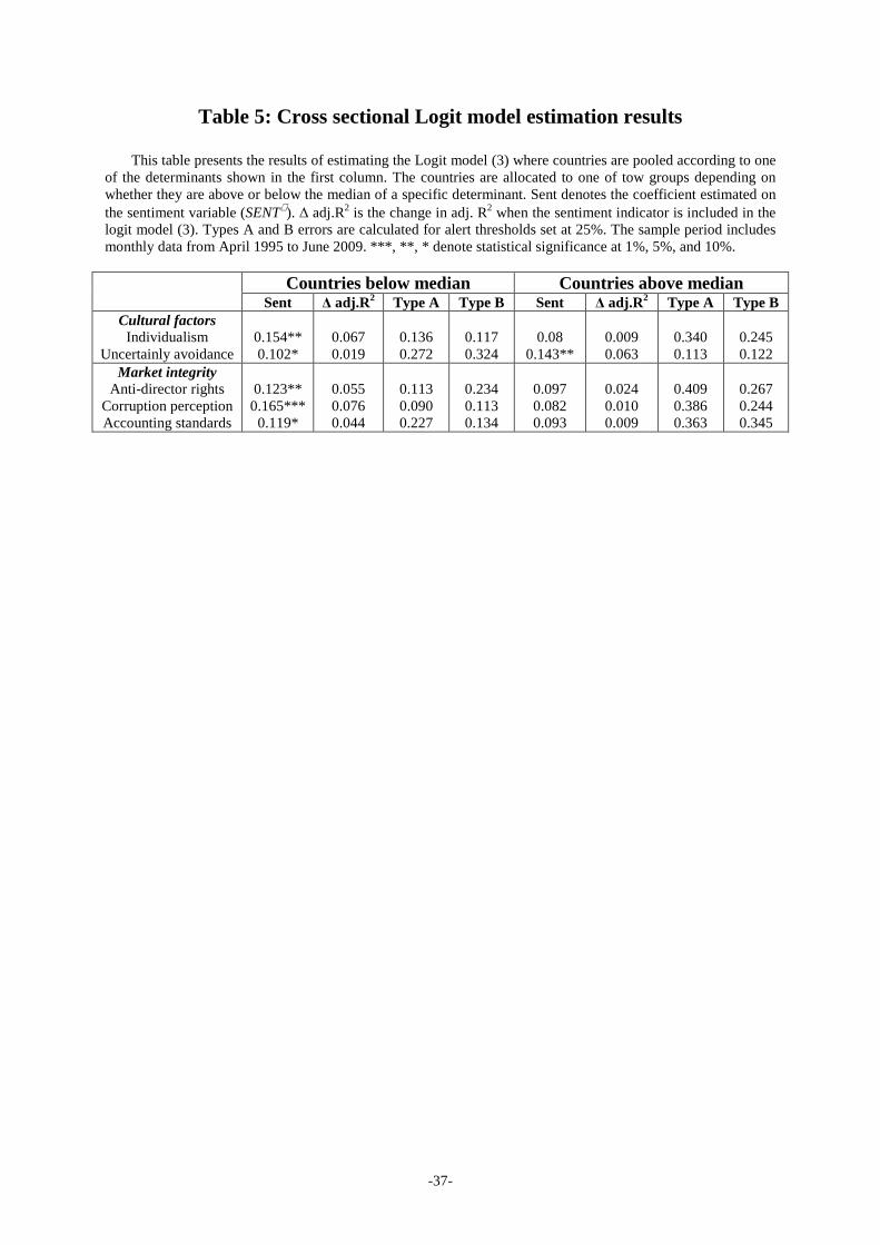
5. Cross-country analyses We examine whether our results are sensitive to the countries been allocated in two
groups depending on some determinants of market integrity and herd-like overreaction.
Specifically, we use our cross-section of countries to determine if there is evidence that the
impact of sentiment on stock market crises is higher for countries with less market integrity
and for countries culturally prone to overreaction-like behavior and herd behavior.
Market integrity means that financial markets with higher level of institutional
sophistication are characterized by a better flow of information and are consequently more
efficient. The market integrity variables retained in our study can be found in La Porta,
Lopez-de-Silanes, Shleifer and Vishny (1998), Chui, Titman and Wei (2008) and Schmeling
(2009). These variables include (i) the index of anti-director rights, (ii) the corruption
perception index and (iii) the accounting standards index14.
The variables used to assess herd-like overreaction are rooted in the article of Hofstede
(2001). The first index measures the level of individualism of a country and the second one,
the so-called uncertainty avoidance index, measures individual’s attitude toward new and
13 For Denemark, the out-of-sample predicted probability of a crisis in the following 12 months is below the 25% threshold. Detailed results are available upon request. 14 In order to make results easier to interpret, we have rescaled all market integrity indicators. Higher value indicates higher market integrity.
-24-
unexpected occurrences. According to Hofstede (2001), individualism affects the degree to
which people display an independent behavior rather than a dependent behavior. The author
argued that children in collectivistic cultures build their identity from their social system. He
showed that higher levels of collectivism indicate a tendency towards herd like behavior. The
uncertainty avoidance index measures the degree to which a culture programs its members to
react to new and unusual situations. Hofstede (2001) documented that people in countries
with high uncertainty avoiding levels react in a more emotional way compared to countries
with low levels of uncertainty avoidance. Therefore we use the uncertainty avoidance as a
proxy of the tendency of individuals to overreact. Hofstede (2001) showed that the
uncertainty avoidance index is correlated with the collectivism index since the uncertainty
avoidance index captures cross-country differences in the propensity of people to follow the
same sets of rules and thus to behave in the same manner. Therefore, higher levels of the
uncertainty avoidance behavior should indicate a tendency towards more herd-like behavior.
Findings are depicted in Table 5.
[INSERT TABLE 5]
For both groups of countries, the McFadden R2 is higher when sentiment is added in the
model. However, results show that the variable SENT⊥ is only significant for the group of
countries showing high herd-like behavior and low market integrity. For the other group,
SENT⊥ is significant when the index uncertainty avoidance is used. Furthermore, the model
quality is good. We find that the errors of types A and B are lower for collectivistic countries,
countries with high uncertainty avoiding index and countries with low institutional
involvement.
Findings show that using the variable sentiment improves our ability to predict stock
prices departure from their fundamental values in countries where herd-like behavior and
overreaction behavior are strong and where market integrity is low. The evidence in the table

-25-
indicates that culture has a different effect on stock market crises, a result consistent with the
idea that investors in different cultures have different biases.
6. Investor sentiment as a predictor of reversals market points
Results so far indicate that the introduction of a sentiment indicator improves our forecast
of stock market crises. From the viewpoint of the investor, however, it is more important to
identify the turning point of the market then the moment when falling prices have reached an
abnormally low level.
Contrary to previous studies on investors’ sentiment, our methodology can be adjusted to
study the market reversals points. Specifically, we use the dates of peaks previously
determined to detect the turning points of the stock markets. As with the prediction of stock
market crises, we construct an binary indicator PRi,t15. The indicator takes the value of 1 for
the month corresponding to the top of the index and the twelve months before the top and 0
otherwise. The 11 months following the peak are excluded from the sample. Our model is
now adapted to identify these stock market reversals points. Table 5 summarizes findings.
[INSERT TABLE 6]
Sentiment indicator is positively correlated with the probability that asset prices reach
their highest level within a one-year horizon. In other words, when our model includes a
sentiment indicator it predicts the potential of triggering a stock market crisis in the next 12
with more accuracy than when only traditional financial and macroeconomic indicators are
used. Financial crises are often preceded by excess optimist leading to value securities above
their fundamental values. The euphoria of investors drives up stock prices leading to financial
crises within a one-year horizon.
15 We use the model of Coudert and Gex (2008).

-26-
The introduction of variable sentiment improves the prediction of turning points both in
terms of quality of regression or quality forecasting. Notice however that these results must be
interpreted with caution. Indeed, the percentages of errors of types A and B are relatively
large and the McFadden R2 does not exceed 14.2%. Thus, predicting stock market reversals
provides weaker performance than forecasting crises.
Conclusion
The general finding of a sentiment-return relation is at odds with standard finance theory
which predicts that stock prices reflect the discounted value of expected cash-flows and that
irrationalities among market participants are erased by arbitrageurs. In contrast, the behavioral
approach suggests that waves of irrational sentiment, i.e. times of overly optimistic or
pessimistic expectations, can persist and affect asset prices for significant periods of time,
eventually generating crises. This paper attempts to assess the relationship between investor
sentiment and stock market crises.
Specifically, our paper empirically examines the influence of investor sentiment on the
probability of occurrence of stock market crises over the period 1995-2009. We use panel data
of 15 European countries and the United States to estimate a multivariate logit model. It
appears that the sentiment of investors positively influence the probability of occurrence of
stock market crises within a one-year horizon. Furthermore, the investor sentiment provides
an incremental predictive power compared to other variables routinely used in the literature.
The impact of investor sentiment on stock markets is stronger for countries that culturally
more prone to herd-like behavior and overreaction and countries with low efficient regularity
institutions. This result is important for portfolio managers; investors’ sentiment is a good
predictor of securities overvaluation. Finally, this is a key result for financial market
regulators, investors’ sentiment can be useful to anticipate stock market crisis.

-27-
References Ang, Andrew, and Geert Bekaert, 2007, Stock return predictability: is it there?, Review of
Financial Studies 20, 651-707. Baker, Malcolm, and Jeffrey Wurgler, 2006, Investor Sentiment and the Cross-Section of
Stock Returns, Journal of Finance 61, 1645-1680. Baker, Malcolm, and Jeffrey Wurgler, 2007, Investor Sentiment in the Stock Market, Journal
of Economic Perspectives 21, 129-151. Baker, Malcolm, Jeffrey Wurgler, and Yu Yuan, 2009, Global, Local, and Contagious
Investor Sentiment, National Bureau of Economic Research (NBER). Barberis, Nicholas, Andrei Shleifer, and Robert Vishny, 1998, A model of investor sentiment,
Journal of Financial Economics 49, 307-343. Baur, Michael N, Socorro Quintero, and Eric Stevens, 1998, The 1986-1988 Stock Market :
Investor sentiment or fundamentals?, Managerial and Decision Economics 17, 319-329.
Berg, Andrew, and Catherine Pattillo, 1999, Are Currency Crises Predictable? A Test, IMF Staff Papers 46, 107-138.
Black, Fischer, 1988, An equilibrium Model of the Crash NBER Macroeconomics Annual, 3, 269-275.
Black, Fischer, 1986, Noise, Journal of Finance 41, 529-543. Blanchard, J. Olivier, 1993, Mouvement in the equity premium, Brookings Papers on
Economic Activity. Bordo, Michael D., and David C. Wheelock, 1998, Price Stability and Financial Stability: The
Historical Record, Federal Reserve Bank of St.Louis Review Sep/Oct., 41-62. Borio, Claudio, and Philip Lowe, 2002, Asset Prices, Financial and Monetary Stability:
Exploring the Nexus, BIS Working Papers n°114. Boucher, Christophe, 2004, Identification et comparaison des crises boursières, Conseil
d’Analyse Economique, report, 50, 375-396. Brown, Gregory W., and Michael T. Cliff, 2004, Investor sentiment and the near-term stock
market, Journal of Empirical Finance 11, 1-27. Brown, Gregory W., and Michael T. Cliff, 2005, Investor Sentiment and Asset Valuation,
Journal of Business 78, 405-440. Bussiere, Matthieu, and Marcel Fratzscher, 2006, Towards a new early warning system of
financial crises, Journal of International Money & Finance 25, 953-973. Campbell, John, and Robert Shiller, J, 2001, Valuation Ratios and the Long-Run Stock
Market Outlook: An Update, National Bureau Of Economics Research Working Paper 8282.
Charoenrook, Anchada, 2006, Does Sentiment Matter?, Vanderbilt University. Chui, Andy C.W., Sheridan Titman, and K. C. John Wei, 2008, Individualism and Momentum
Around the World, Journal of Finance, forthcoming. Clarke, Roger G., and Meir Statman, 1998, Bullish or Bearish?, Financial Analysts Journal
54, 63-166. Cutler, David M., James M. Poterba, and Lawrence H. Summers, 1991, Speculative
Dynamics, Review of Economic Studies 58, 529-547. Corsetti, Giancarlo, Paolo Pesenti, and Nouriel Roubini, 1999, Paper tigers? A model of the
Asian crisis, European Economic Review 43, 1211-1236. Coudert, Virginie., and Mathieu. Gex. 2008. Does risk aversion drive financial crises? Testing
the predictive power of empirical indicators. Journal of Empirical Finance 15 (2):167-184.
-28-
Daniel, Kent D., David Hirshleifer, and Avanidhar Subrahmanyam, 2001, Overconfidence, Arbitrage, and Equilibrium Asset Pricing, Journal of Finance 56, 921-965.
De Long, J. B., and A. Shleifer, 1991, The stock market bubble of 1929: Evidence from closed-end mutual funds, Journal of Economic History 51, 675-700.
De Long, J. Bradford, Andrei Shleifer, Lawrence H. Summers, and Robert J. Waldmann, 1990, Noise trader risk in financial markets, Journal of Political Economy 98, 703-738.
Demirgüc-Kunt, Asli;, and Enrica; Detragiache, 2000, Monitoring Banking Sector Fragility : A Multivariate Logit Approach, The World Bank Economic Review 14, 287-307.
Fama, Eugene F., 1989, Perspectives on octobre 1989 Or What did we learn from the crash? , Black Mondy and the Future of Financial Market 71-82.
Fama, Eugene, and G.William Schwert, 1977, Asset Returns and Inflation, Journal of Financial Economics 5, 115-146.
Fisher, Kenneth L., and Meir Statman, 2000, Investor Sentiment and Stock Returns, Financial Analysts Journal 56, 16-23.
Fisher, Kenneth L., and Meir Statman, 2003, Consumer Confidence and Stock Returns, Journal of Portfolio Management 30, 115-127.
Frankel, Jeffrey A., and Andrew K. Rose, 1996, Currency Crashes in Emerging Markets: An Empirical Treatment, Working Papers --US Federal Reserve Board's International Finance Discussion Papers.
Glushkov, Denys, 2006, Sentiment beta, University of Texas at Austin. Goldstein, Morris, 1998, The Asian Financial Crisis: Causes, Cures, and Systematic
Implications, Institute of International Economics: Washington, DC. 77 pages, Goodfriend, Marvin 2001, Financial stability, deflation and monetary policy, Bank of Japan,
Special Edition, February. Kamin, Steven B., 1999, The current international financial crisis: how much is new?,
Federal Reserve System. Kaminsky, Graciela, Saul Lizondo, Carmen M. Reinhart, 1998, Leading indicators of
currency crises, IMF Staff Papers 45, 1-48. Kumar, Alok, and Charles M. C. Lee, 2006, Retail Investor Sentiment and Return
Comovements, Journal of Finance 61, 2451-2486. La Porta, Rafael, Florencio Lopez-de-Silanes, Andrei Shleifer, and Robert W. Vishny, 1998,
Law and finance, Journal of Political Economy 106, 1113-155. Lau, Lawrence J., and Isabel K. Yan, 2005, Predicting Currency Crises With A Nested Logit
Model, Pacific Economic Review 10, 295-316. Lee, Charles M. C., Andrei Shleifer, and Richard H. Thaler, 1991, Investor Sentiment and the
Closed-End Fund Puzzle, Journal of Finance 46, 75-109. Lee, Yul W., and Zhiyi song, 2003, When do Value Stocks Outperform Growth Stocks?
Investor Sentiment and Equity Style Rotation Strategies, University of Rhode Island - Area of Finance and Insurance.
Lemmon, Michael, and Evgenia Portniaguina, 2006, Consumer Confidence and Asset Prices: Some Empirical Evidence, Review of Financial Studies 19, 1499-1529.
Maddala, G.S, 1983, Limited Dependent and Qualitative Variables in Econometrics, Cambridge University Press.
Neal, Robert, and Simon M. Wheatley, 1998, Do measures of investor sentiment predict returns?, Journal of Financial & Quantitative Analysis 33, 523-547.
Nelson, Charles.R, 1976, Inflation and rates of return on common stocks, The journal of Finance 47, 1591-1603.
Niederhoffer, Victor, 1971, The Analysis of World Events and Stock Prices, Journal of Business 44, 193-219.

-29-
Otoo, Maria., 1999, Consumer Sentiment and The Stock Market, Federal of Reserve System. Patel, Sandeep A., and Asani Sarkar, 1998, Crises in Developed and Emerging Stock
Markets, Financial Analysts Journal 54, 50-61. Qiu, Lily, and IVO Welch, 2006, Investor Sentiment Measures, Brown University and NBER. Roll, Richard, 1988, The international Crash of October 1987, Financial Analysts Journal 44,
19-35. Rubinstein, Mark, 2001, Rational Markets: Yes or No? The Affirmative Case, Financial
Analysts Journal 57, 15-29. Schmeling, Maik, 2009, Investor sentiment and stock returns: Some international evidence,
Journal of Empirical Finance 16, 394-408. Schmitz, Philipp., Markus. Glaser, and Martin. Weber, 2007, Individual Investor Sentiment
and Stock Returns - What Do We Learn from Warrant Traders?, University of Mannheim - Department of Banking and Finance.
Seyhun, H. Nejat, and Douglas J. Skinner, 1994, How do taxes affect investors' stock market realizations? Evidence from tax-return panel data, Journal of Business 67, 231-262.
Shefrin, Hersh. , 2005, A Behavioral Approach To Asset Pricing Burlington, MA: Elsevier Academic Press. .
Shiller, Robert, J, 1987, Investor Behaviour in the October 1987 Stock Market Crash: Survey Evidence, National Bureau Of Economics Research Working Paper.
Shiller, Robert J., 1989, Market Volatility, Cambridge, Mass MIT Press. Shiller, Robert J., 2000. Irrational Exuberance. Broadway Books Shleifer, Andrei, 2000, Inefficient Markets: An Introduction to Behavioral Finance in inc.
Oxford University Press, ed.: (New York). Siegel, Jeremy J., 1992, Equity risk premia, corporate profit forecasts, and investor sentiment
around the stock crash of October 1987, Journal of Business 65, 557-570. Solt, Michael E., and Meir Statman, 1988, How Useful is the Sentiment Index?, Financial
Analysts Journal 44, 45-55. Thaler, Richard H., 1999, The End of Behavioral Finance, Financial Analysts Journal 55, 12-
17. White, Eugene N., 1990, The Stock Market Boom and Crash of 1929 Revisited, Journal of
Economic Perspectives 4, 67-83.
Annexe 1
The data stock market indices, mainly drawn from the Datastream database for the period
1995-2008, are the following : BEL 20 (Belgium), PRAGUE PX 50 (Czech Republic), OMX
Copenhagen (Denmark), DAX 30 (Germany), HE GENERAL IRELAND (Ireland), ATHENS
SE GENERAL (Greece), IBEX 35 (Spain) , CAC 40 (France), 30 MILAN COMIT (Italy),
ESTONIA TALS INDEX (Estonia), PORTUGAL PSI-20 (Portugal), SLOVENIAN EXCH.
STOCK (Slovenia), DJWI FINLAND (Finland), SWEDEN OMX (Sweden), FTSE 100 (UK)
and the S&P 500 Composite (U.S.). The PER and dividend yield on stock indices are
extracted from Bloomberg.

-30-
The inflation data (change in the consumer prices index), the real interest rate (the money
market rate using the consumer price index), the industrial production, the term structure, the
GDP16 and consumption expenditures are all taken from the IMF’s International Financial
Statistics (IFS). The time series of domestic bank credit come from the European Central
Bank (ECB) for the European countries. The source is the U.S. Federal Reserve for the United
States. The consumer confidence indices are provided by the Economic European
Commission for the countries of the European countries. The source is the University of
Michigan Survey Research Center for the U.S. consumer confidence. All time series used are
seasonally adjusted.
Annexe 2
The consumer confidence index is the result of a survey of a representative population of
households. It reflects the perceptions and expectations of households both on their economic
and financial situation as their propensity to spend and their views on the overall economic
situation. The survey consists of simple questions with multiple choice answers are easily
recognized. The relative score of each question is then calculated as the percent of favourable
replies minus the percent of unfavorable replies, plus 100, rounded to the nearest whole
number. The Michigan surveys are sent to households and the respondents are asked the
following questions:
Q1. Do you think now is a good time for people to buy major household items?
• good time to buy • uncertain • depends • bad time to buy
Q2. Would you say that you and your immediate family are better off or worse off financially
than you were a year ago?
16 Quarterly data have been transformed into monthly data using moving averages.

-31-
• better • same • worse
Q3. Now turning to business conditions in the country as a whole-do you think that during
the next twelve months the financial condition will be?
• good • uncertain • bad
Q4. Looking at the next five years, do you think we will continue having?
• good times • uncertain • bad times
Q5. A year from now, do you think your immediate family will be?
• better • same • worse
-32-
Table 1: Description of variables used in the study
Code Variables Measures Sources Macroeconomics variables
INT Real interest rate Money market rate using consumer price
index International Financial Statistics
INF Inflation Change in the natural logarithm of the
Consumer Price Index International Financial Statistics
CREDIT/GDP Domestic credit Level of domestic credit divided by Gross
Domestic Product European central Bank & Federal reserve
system
ST Term spread Difference between the yields on 10-year
U.S. government bonds and 3-month Treasury bills
International Financial Statistics
IP Industrial production Change in the natural logarithm of
industrial production index International Financial Statistics
CD, CND et CS Growth of durable goods, non-durables
goods and services consumption expenditures
Change in the natural logarithm of durable goods, non-durables and services
consumption expenditures International Financial Statistics
Stock market variables P Stock price index Level of stock price index Datastream
PER Price Earning Ratio Share price divided by earning per share Bloomberg
DY Dividend Yield Cash dividend of the index divided by the
value of the index Bloomberg
RET The year-one-year change in stock prices Yearly change in stock prices Datastream Investor sentiment indicator
SENT Consumer sentiment index The five questions making up the consumer
sentiment index
Economic European Commission & University of Michigan Survey Research
Center
-33-
Tableau 2: Characteristics of individual market crises
This table presents the characteristics of the stock market crises. The beginning of a crisis is the month when the index reaches its historical maximum over the 2-year window prior to the month when the crash is triggered. The beginning of the crash corresponds to the month when the CMAX intersects with a threshold. The date of trough is the month when the price index reaches its minimum. The date of recovery is the first month after the crash when the index reaches the pre-crash maximum. The magnitude of a crisis is the difference between the value of the index at its maximum and at its minimum. The length of the trough is the number of months between the date of the beginning of the crisis and the date of the trough. The length of the recovery period is the number of months for the index to return to the maximum. To avoid counting the same crisis more than once, a crisis is automatically eliminated if detected twice over a twelve month period.
The duration of the crisis
Annual returns before crises
Annual returns after crises
Beginning of crises
Beginning of crash
Date of trough
Date of recovery
Month to trough
Month to recovery
Price decline to trough
One year
Three years
One year
Three years
Belgium 10/2000 09/2002 03/2003 05/2005 29 26 46.49% 0.793% 5.09% 20.45% 22.92% 05/2007 06/2008 03/2009 NA 13 NA 66.77% 27.80 % 53.94 % NA NA
Czech Republic 05/1994 06 /1995 07/1995 03/2004 14 105 44.98% NA NA 54.96% 110.25% 11/2007 10/2008 03/2009 NA 11 NA 66.41% 24.03 % 109.26 % NA NA
Denmark 10/2000 07/2002 02/2003 01/2005 28 23 43.83% 43.23% 59.76% 36.33% 63.48% 10/2007 09/2008 03/2009 NA 17 NA 57.77% 24.80% 49.48% NA NA
Germany 02/2000 09/2001 09/2002 NA 31 NA 67.26% 55.09% 87.98% NA NA 10/2000 10/2002 03/2003 NA 17 NA 66.86% 22.72 % 84.73% NA NA 10/2007 10/2008 02/2009 NA 16 NA 54.48% 32.33% 76.25% NA NA
Ireland 06/2001 06/2002 03/2003 12/2005 21 33 55.13% 21.24% 31.92% 29.87% -44.02% 05/2007 07/2008 02/2009 NA 21 NA 62.17% 35.24% 87.67% NA NA
Greece 11/1999 09/2001 09/2002 NA 22 NA 62.12% 98.27% 127.53% NA NA 04/2001 03/2003 03/2003 09/2005 23 30 55.35% -32.64% 20.99% 16.23% -15.53% 10/2007 10/2008 02/2009 NA 16 NA 71.20% 29.20% 114.30% NA NA
Spain 02/2000 08/2001 07/2002 09/2006 29 50 33.88% 25.89% 137.22% 11.94% -9.11% 09/2000 09/2002 09/2002 07/2005 24 34 50.39% 14.95% 50.62% 16.82% 17.45% 11/2007 10/2008 02/2009 NA 15 NA 51.64% 13.97% 81.29% NA NA

-34-
Tableau 2: Characteristics of individual market crises
This table presents the characteristics of the stock market crises. The beginning of a crisis is the month when the index reaches its historical maximum over the 2-year window prior to the month when the crash is triggered. The beginning of the crash corresponds to the month when the CMAX intersects with a threshold. The date of trough is the month when the price index reaches its minimum. The date of recovery is the first month after the crash when the index reaches the pre-crash maximum. The magnitude of a crisis is the difference between the value of the index at its maximum and at its minimum. The length of the trough is the number of months between the date of the beginning of the crisis and the date of the trough. The length of the recovery period is the number of months for the index to return to the maximum. To avoid counting the same crisis more than once, a crisis is automatically eliminated if detected twice over a twelve month period.
The duration of the crisis
Annual returns before crises
Annual returns after crises
Beginning of crises
Beginning of crash
Date of trough
Date of recovery
Month to trough
Month to recovery
Price decline to trough
One year
Three years
One year
Three years
France 08/2000 09/2001 09/2002 NA 25 NA 38.43% 44.36% 139.14% NA NA 10/2000 10//2002 03/2003 NA 29 NA 50.76% 30.86% 133.55% NA NA 05/2007 10/2008 02/2009 NA 21 NA 55.72% 23.80% 66.33% NA NA
Italy 08/2000 09/2001 09/2002 NA 25 NA 55.02% 42.66% 124% NA NA 10/2000 10/2002 03/2003 NA 29 NA 53.86% 44.27% 119.17% NA NA 05/2007 10/2008 02/2009 NA 21 NA 62.09% 18.71% 56.96% NA NA
Estonia 08/1997 06/1998 12/1998 12/2004 16 72 81.59% 133.53% NA 47.96% 41% 10/1997 07/1999 10/1999 03/2004 24 53 67.74% 152.22% NA 79.76% 164% 01/2007 06/2008 02/2009 NA 25 NA 58.27% 52.85% 165.24% NA NA
Portugal 02/2000 07/2001 07/2002 NA 29 NA 58.03% 30.23% 140.67% NA NA 08/2000 08/2002 03/2003 04/2007 31 65 55.80% 20.86% 59.80% NA NA 07/2007 10/2008 02/2009 NA 29 NA 55.30% 38.99% 88.50% NA NA
Slovenia 06/1994 05/1996 07/1996 03/1998 25 20 41.67% 35.10% NA 10.73% 6.10% 07/2007 02/2008 04/2008 NA 9 NA 30.96% 116.20% 145.16% NA NA 09/2007 03/2009 03/2009 NA 18 NA 70.08% 115.81% 149.90% NA NA
Finland 04/2000 02/2001 09/2001 NA 17 NA 67.48% 165.15% 195.23% NA NA 06/2000 06/2002 07/2004 NA 49 NA 72.91% 103.58% 123.87% NA NA 10/2007 11/2008 02/2009 NA 16 NA 67.20% 44.54% 104.05% NA NA

-35-
Tableau 2: Characteristics of individual market crises
This table presents the characteristics of the stock market crises. The beginning of a crisis is the month when the index reaches its historical maximum over the 2-year window prior to the month when the crash is triggered. The beginning of the crash corresponds to the month when the CMAX intersects with a threshold. The date of trough is the month when the price index reaches its minimum. The date of recovery is the first month after the crash when the index reaches the pre-crash maximum. The magnitude of a crisis is the difference between the value of the index at its maximum and at its minimum. The length of the trough is the number of months between the date of the beginning of the crisis and the date of the trough. The length of the recovery period is the number of months for the index to return to the maximum. To avoid counting the same crisis more than once, a crisis is automatically eliminated if detected twice over a twelve month period.
The duration of the crisis Annual returns before
crises Annual returns after
crises Beginning of crises
Beginning of crash
Date of trough
Date of recovery
Month to trough
Month to recovery
Price decline to trough
One year
Three years
One year
Three years
Sweden 04/2000 08/2001 08/2002 NA 28 NA 63.21 % 84% 174.69% NA NA 09/2000 08/2002 03/2003 04/2007 30 49 60.94 % 46.35% 86.59% NA NA 05/2007 06/2008 01/2009 NA 20 NA 75.43 % 34.62% 86.16% NA NA
United Kingdom 08/2000 09/2001 09/2002 10/2007 25 61 44.22 % 2.13% 29.70% NA NA 10/2000 10/2002 03/2003 07/2007 29 52 43.87 % 2.92% 32.96% NA NA 05/2007 09/2008 02/2009 NA 21 NA 41.96 % 15.68% 47.48% NA NA
United States 07/2000 07/2001 06/2002 04/2007 23 58 39.99 % 14.94% 68.73% -8.50% NA 08/2000 08/2002 08/2002 12/2006 24 52 43.24 % 11.99% 51.64% -22.46% NA 09/2007 06/2008 02/2009 NA 17 NA 52.55 % 12.44% 37.08% NA NA

-36-
Table 4: Results of the Logit model estimation - stock market crises
This table presents the results of the Logit model. The dependent variable equals 1 for the 12 months preceding the crisis, and 0 during quiet periods. The 11 months following the crisis are excluded from the sample. The independent variables represent the real interest rate (INT), the year-one-year change in stock prices (RET), the Price Earnings Ratio (PER), the inflation (INF), the ratio domestic credit to GDP (CREDIT) and the investor
sentiment (SENT⊥). The statistics tabulated in parentheses correspond to the p-values. The sample period includes monthly data from April 1995 to June 2009. ***, **, * denote statistical significance at 1%, 5%, and 10%.
Explanatory Variables Model 1 Model 2 Model 3
Constant -1.234*** (-0.002)
-2.567*** (-0.000)
-2.276*** (-0.000)
INT -0.112* (-0.07)
-0.089** (-0.041)
RET -2.278** (-0.022)
-2.345** (-0.034)
PER 0.024* (0.079)
0.005
(0.265)
INF -3.856** (-0.031)
-3.983** (-0.03)
CREDIT 0.877*** (0.006)
0.676*** (0.000)
SENT⊥ 0.157** (0.031)
0.134** (0.041)
R2 McFadden LR stat
0.401 (0.000)
0.082 (0.000)
0.462 (0.000)
Forecast error (%) Seuil de 50 %
Type A(1)
Type B(2)
35.714 15.213
52.227 13.278
27.272 12.789
Seuil de 25 % Type A(1)
Type B(2)
29.545 21.678
31.818 16.212
18.181 17.289
(1) Probability of crisis given no alarm. (2) Percentage of false alarms.
-37-
Table 5: Cross sectional Logit model estimation results
This table presents the results of estimating the Logit model (3) where countries are pooled according to one of the determinants shown in the first column. The countries are allocated to one of tow groups depending on whether they are above or below the median of a specific determinant. Sent denotes the coefficient estimated on the sentiment variable (SENT⊥). ∆ adj.R2 is the change in adj. R2 when the sentiment indicator is included in the logit model (3). Types A and B errors are calculated for alert thresholds set at 25%. The sample period includes monthly data from April 1995 to June 2009. ***, **, * denote statistical significance at 1%, 5%, and 10%.
Countries below median Countries above median Sent ∆ adj.R2 Type A Type B Sent ∆ adj.R2 Type A Type B
Cultural factors Individualism
Uncertainly avoidance
0.154** 0.102*
0.067 0.019
0.136 0.272
0.117 0.324
0.08
0.143**
0.009 0.063
0.340 0.113
0.245 0.122
Market integrity Anti-director rights
Corruption perception Accounting standards
0.123** 0.165*** 0.119*
0.055 0.076 0.044
0.113 0.090 0.227
0.234 0.113 0.134
0.097 0.082 0.093
0.024 0.010 0.009
0.409 0.386 0.363
0.267 0.244 0.345

-38-
Table 6: Results of the Logit model estimation - stock market reversals points
This table presents the results of the Logit model. The dependent variable equals 1 for the 12 months preceding the crisis, and 0 during quiet periods. The 11 months following the crisis are excluded from the sample. The independent variables represent the real interest rate (INT), the year-one-year change in stock prices (RET), the Price Earnings Ratio (PER), the inflation (INF), the ratio domestic credit to GDP (CREDIT) and the investor
sentiment (SENT⊥). The statistics tabulated in parentheses correspond to the p-values. The sample period includes monthly data from April 1995 to June 2009. ***, **, * denote statistical significance at 1%, 5%, and 10%.
Explanatory Variables Model 1 Model 2 Model 3
Constant 2.009*** (0.003)
0.895 (0.08)
1.878*** (0.000)
INT 0.223** (0.055)
0.211** (0.054)
RET 0.289* (0.078)
0.287** (0.088)
PER 0.376** (0.025)
0.099
(0.343)
INF -0.021** (-0.045)
-0.020** (-0.048)
CREDIT 0.871*** (0.007)
0.814*** (0.000)
SENT⊥ 0.133* (0.067)
0.123* (0.086)
R2 McFadden LR stat
0.123 (0.003)
0.021 (0.015)
0.142 (0.005)
Forecast error (%) Seuil de 50 %
Type A(1)
Type B(2)
68.181 53.367
84.090 73.876
52.272 57.134
Seuil de 25 % Type A(1)
Type B(2)
56.818 62.298
75.000 82.989
45.454 74.435
(1) Probability of crisis given no alarm (2) Percentage of false alarms of total alarms