DISCUSSION PAPER SERIES DPS16.27 NOVEMBER 2016

How does early deprivation relate to later-life outcomes? A longitudinal analysis Ron DIRIS and Frank VANDENBROUCKE Public Economics

Faculty of Economics and Business

How does early deprivation relate to later-life outcomes?

A longitudinal analysis

Ron Diris* and Frank Vandenbroucke†

Abstract

Measures of material deprivation are increasingly used as alternatives to traditional poverty

indicators. While there exists extensive literature focusing on the impact that growing up in a

(financially) poor household has on future success, little is known about how material depri-

vation relates to long-run outcomes. This study uses longitudinal data from the 1970 British

Cohort Study to assess the relationship between material deprivation and outcomes in adult

life. We control for an extensive set of observable characteristics, and further employ value-

added analysis and generalized sensitivity analysis to assess the nature of this relationship.

We find that deprivation relates to a diverse set of outcome variables, but the magnitude of

the conditional relationships are generally small. Immaterial indicators of family quality show

relatively stronger ties to future outcomes, especially with respect to non-cognitive skills.

Keywords: material deprivation, long-run outcomes, poverty, family disadvantage

JEL Classification: I32, J13, J62

*Department of Economics, Maastricht University, 6200 MD Maastricht, the Netherlands,r.diris@maastrichtuniversity.nl (corresponding author)

†University of Amsterdam, KU Leuven and University of Antwerp.We would like to thank Erwin Ooghe, Brian Nolan, Geranda Notten, Kristof de Witte, the participants of the 2016APPAM conference in London and the participants of the PE seminar in Leuven for their helpful comments.

1

1 Introduction

Classifications of poverty or social exclusion have traditionally relied on measures of individual

or household income. Material deprivation (MD) is increasingly used as an alternative indicator

for social exclusion. MD indicators refer to a list of ’basic necessities’ for households in different

domains of life. The increasing use of these indicators reflects the perception that social exclusion

captures more than a lack of income. Although MD depends on what is perceived as a basket of

necessities at a given point in time, it is essentially an absolute measure of poverty. This contrasts

with the commonly used at-risk-of-poverty rate, which reflects relative income positions within a

country.1 MD indicators have become popular as indicators of social exclusion in international

or intertemporal comparisons. ‘Severe material deprivation’ is included in the poverty and so-

cial exclusion target of the Europe 2020 strategy of the European Union (European Commission,

2010). However, in contrast to income poverty, little is known about how growing up in material

deprivation is specifically related to important measures of later-life success.

This study analyzes the relationship between growing up in a household confronted with mate-

rial deprivation and later-life outcomes. We use data from the British Cohort Study (BCS), which

follows a total of 17,000 individuals born in Britain in the first week of April 1970. The BCS re-

ports extensive information on the child and its parents at birth and contains follow-ups at multiple

ages in both childhood and adult life, until an age of 42. It provides extensive data on household

possessions and circumstances as well as a vast range of outcome variables for several measures

of social progress in adult life. We extensively assess to what extent raw correlations between

deprivation and future outcomes are driven by associations with other determinants of deprivation

and social progress. Moreover, we use value-added analysis and generalized sensitivity analysis as

developed by Imbens (2003) to further address selection bias and to establish whether it is likely

that a causal relationship remains. Using factor analysis, we establish six different domains of

1The contrast between the absolute character of MD and the relative character of income poverty indicators shouldbe interpreted with nuance. Poverty indicators can also have an absolute character, at least within the context of onecountry, when the poverty threshold is anchored in time. However, this is based on an arbitrary choice of the baseyear (in which the threshold is defined). It is, in principle, also possible to use material deprivation data to constructindicators of relative material deprivation within countries. However, as Notten and Roelen (2012) show, constructingrelative measures on the basis of MD is a hazardous exercise.

2

material deprivation for which these relationships are estimated.

The study is related to two different strands of literature: studies analyzing material deprivation

as an alternative (or complementary) measure of poverty and studies that assess the relationship

between family background and important later-life outcomes. The former group of studies mainly

focuses on explaining the mismatch between being income-poor and being materially deprived,2

and on how to construct one encompassing measure of material deprivation from the total set of

domains and items.3 Advocates of the use of MD emphasize its benefits over poverty indicators that

are strictly based on income, both from a conceptual point of view (income neglects circumstances,

preferences and risk factors) and in terms of measurement (yearly income measures are volatile

across time and prone to measurement error, especially at the extremes of the income distribution).

The literature on the relationship between family circumstances and future outcomes shows

that the family that one is born into matters greatly for success in life. There are strong ties be-

tween the outcomes of parents and the outcomes of their children in later life, for example in terms

of educational attainment and income.4 Evidence from adoption studies indicates that variation

in outcomes between children from different families is not solely due to genes, and therefore

‘family quality’ is of crucial importance for the future social progress of children.5 However, it is

still unclear which specific aspects of the family capture that quality. Studies have used composite

socio-economic status (SES) indicators that typically combine data on parental education, parental

occupation, home possessions and/or parental income, and linked those to several later-life out-

comes.6 Brooks-Gunn and Duncan (1997) provide an overview of studies that specifically focus

on income poverty in relation to child outcomes and conclude that poverty early in life (preschool

and early school years) is most strongly related to important future outcomes.

However, it remains difficult to empirically disentangle the impact of parental education, occu-

2See, e.g., Perry (2002); Whelan et al. (2004).3Different methods are used to elicit one single construct of MD, such as prevalence weighting, principal compo-

nent analysis, item response theory and structural equation modeling, but no consensus exists. For examples of eachof these approaches, see, e.g., Cappellari and Jenkins (2006); Whelan and Maıtre (2005); Tomlinson et al. (2008). Anoverview is provided by Nolan and Whelan (2010).

4See, e.g., Corak (2013) for an overview of the intergenerational transmission of income and, e.g., OECD (2015)for an overview on the relationship between socio-economic background and educational attainment

5See, e.g., Bjorklund et al. (2006); Sacerdote (2008); Beckett et al. (2006).6See, e.g., Bradley and Corwyn (2002) for an overview.

3

pation or income from other aspects that relate to both family background and important life out-

comes, such as school quality, neighbourhood characteristics, child rearing behavior, etc. Recent

literature has aimed to uncover direct causal links between parental income early in life and future

outcomes. Many of these studies focus on the role of credit constraints in relation to educational

attainment. This type of research typically finds that the role of short-term credit constraints be-

comes limited, at best, once we control for other factors such as school achievement and therefore

concludes that permanent family factors are markedly more important than short-term liquidity

(Heckman, 2000; Carneiro and Heckman, 2003; Dearden et al., 2004; Chevalier et al., 2013). Still,

it remains unclear which permanent family factors are especially important and whether (perma-

nent) income is one of those factors. Several studies have exploited exogenous variation in income

to directly assess its causal impact. For example, Frijters et al. (2005), using sibling fixed effects in

combination with the event of German reunification, identifies a low causal impact of income on

health, while Løken (2010), using the Norwegian oil boom as an exogenous shock, finds no causal

impact of income on educational attainment. Other studies identify comparatively larger estimates

but these are still substantially below what simple correlations suggest; see, e.g., Blanden and

Gregg (2004) (partially based on the same (British) data as in this paper) and Akee et al. (2010).

These results call into question whether the direct provision of income to poor families will lead to

substantial improvements in the future prospects of children growing up in these families. Dearden

et al. (2009) address this question directly through their evaluation of the British EMA program,

which provides students with weekly cash transfers conditional on their school attendance. The

program has strong effects on staying in school, but it is not clear whether this is due to an alle-

viation of credit constraints, or because the conditional transfers reduce the opportunity costs of

education.

Overall, these findings tend to suggest that the strong correlation between household income

and future success is for a large part driven by associations with other variables. This has led

multiple researchers to argue that important aspects of the family are largely immaterial (see, e.g.,

Heckman (2008)). An alternative explanation for the limited direct relation between parental in-

come and important later-life outcomes is that, as advocates of MD measures often argue, income

4

only imperfectly measures the restrictions and opportunities that households face. As such, it is

meaningful to analyze these relationship when material deprivation is used as an indicator of so-

cial exclusion, either as a substitute or a complement to income. Establishing the nature of the

links existing between MD indicators and later-life outcomes is also important given the increas-

ing emphasis put on deprivation measures in policy evaluation, which is likely to lead to policies

that are specifically targeted at reducing deprivation. Identifying the nature of the relations from

deprivation towards later-life outcomes would improve evaluations of the benefits of such targeted

policies.

This is the first study that empirically analyzes the relationship between material deprivation

early in life and long-run outcomes. In general, only few studies have linked MD to key measures

of social progress. Filmer and Pritchett (1999) provide an exception, by conducting a macro-level

analysis in which they link differences in wealth (measured by possessions and the presence of

basic facilities such as drinking water and electricity) to differences in educational attainment.

Relying on rich micro-level longitudinal data, the current study estimates the relationship between

material deprivation in childhood and various outcomes, which are measured up until an age of 42.

Additionally, we add to existing literature by extensively addressing the potentially confounding

impact of other variables, analyzing the likelihood of causal effects, and providing a comparison

to results for family income based on the same sample.

The paper is organized as follows. We introduce theoretical considerations in Section 2. Sec-

tion 3 describes the data, while methodological issues are discussed in Section 4. Section 5 presents

empirical results. Section 6 discusses robustness analyses, and Section 7 concludes.

2 Theory

2.1 Defining material deprivation

In this section, we discuss the theoretical concept of material deprivation and issues that arise when

measuring constructs of material deprivation. There is no clear consensus on the specific defini-

tion of material deprivation. The OECD definition states that “material deprivation refers to the

5

inability for individuals and households to afford consumption goods and activities that are typical

in a certain society at a given point in time, irrespective of people’s preferences with respect to

these items” (OECD, 2007). In other words, MD concerns the lack of being able to afford ‘typ-

ical’ consumption goods. A first major conceptual question is how broad the characterization of

deprivation should be. There exists considerable variation in the literature with respect to the exact

construction of MD indicators. Virtually all studies incorporate items that measure household pos-

sessions and housing conditions. More elaborate indicators also typically include neighbourhood

characteristics, access to a healthy lifestyle and measures of social deprivation. Since the aim of

this study is to assess the relationship between MD and later-life success in its broadest sense, and

since relationships to later-life outcomes are unexplored across domains, we incorporate all these

domains in the empirical analysis. Moreover, since we ultimately want to assess how MD affects

children in their developmental process, we also include measures of consumption goods and activ-

ities that are directly aimed at the child’s learning and development (outside of formal educational

processes such as the school or extra-curricular programs) as an additional domain. As such, we

define six domains of deprivation: possessional deprivation, housing deprivation, neighbourhood

deprivation, health deprivation, educational deprivation and social deprivation.

As already suggested by the formal definition, the ‘material’ aspect of MD is not always strictly

adhered. As we want to assess deprivation in its broadest sense, we also incorporate immaterial

aspects. We make a clear distinction between material and ‘immaterial’ deprivation in the analysis

and the discussion of the results. This distinction is already largely reflected in the subdivision into

domains, since the possession, housing, neighbourhood and health domains are material by nature

while the social deprivation domain is immaterial by nature.7 The educational domain is ambigu-

ous as it can contain both tangible learning tools as well as intangible activities and support. We

thereby divide this domain into a material and an immaterial sub-domain and discuss the results for

each sub-domain separately across the analysis. The two immaterial domains might alternatively

be thought of as cultural and social ‘capital’ (or lack thereof). The conceptual distinction between

7One might argue that aspects of the neighbourhood such as the prevalence of crime and poverty are not material,but since we believe that the neighbourhood is conceptually tied to the household’s living arrangements (which areevidently material and captured by the housing domain), we categorize it under material.

6

the two types of deprivation goes beyond the material aspect, as the immaterial items are typically

more difficult to measure (often depending on subjective interpretations) and one might also not

typically see them as things that everyone ‘should have’. Ermisch (2008) makes a similar distinc-

tion in his analysis of parenting on inequality and labels these aspects as ‘what parents buy’ versus

‘what parents do’. We believe that these immaterial aspects are important to consider in light of

the bigger question on what aspects of family quality matter most, but simultaneously recognize

that we should be aware of these conceptual differences when comparing and interpreting results.

2.2 Measuring material deprivation

Another crucial conceptual question is what type of items within these domains should be included

in each variable. Data availability inevitably determines this to some extent in any empirical ap-

plication, but additional criteria can be employed. First of all, the definition clearly states that the

goods, services or activities should be typical in society, which in this case is Britain in the 1970s

and 1980s. In other words, it should not concern ‘enrichment’ items that are only available to a

limited share of the population. Still, the connotation ‘typical’ leaves room for interpretation. In

this study, we specify the constraint that the item should be available to at least half of the popula-

tion. This could be seen as a rather loose constraint, but we include additional analyses that assess

whether the estimated relationships are different when we limit the indicator to items with higher

prevalence.

Additionally, the formal definition of MD states that the lack of a certain item should be the

result of a lack of affordability rather than preferences. For this reason, items that comprise MD

indicators are often based on questions that distinguish between not having an item because of not

being able to afford it or because of personal preference. However, this study specifically looks at

the impact of deprivation for children, who are not bound by their own preferences but predomi-

nantly by those of their parents. Additionally, affordability is always linked to how an individual

or a household ranks goods and services in terms of value and necessity, and therefore not having

an item can never be seen completely ‘irrespective of preferences’, as the formal definition of MD

7

technically requires.8 Additionally, there are several items for which the distinction is not made

in the data and would also be conceptually odd, such as being situated in a high-crime neighbour-

hood. For these reasons, we do not consider the distinction between affordability and personal

preference when constructing deprivation indicators in our main analysis. We conduct a sensitivity

analysis in a later stage for those items where the distinction is made in the data, in order to assess

to what extent the distinction matters for the results.

A final potential point of concern in assessing the relationship between material deprivation

and a certain outcome is that there are always additional variables that one might have considered

in constructing deprivation but are not available in the data. However, this is a natural conse-

quence of the nature of MD indicators and therefore part of the conceptual difference with a more

‘concise’ measure of poverty, such as income. Since we rely on a very extensive dataset in the

empirical analysis, the MD indicators we employ are comparatively very rich. Hence, although

our estimates are essentially lower bounds due to the fact that there is a potentially inexhaustible

list of relevant items one could include, they might be viewed as upper bounds of what MD can

explain in empirical studies.

3 Data

The analysis in this study is based on data from the 1970 British Cohort Study, which follows

all individuals born in Britain in the first week of April 1970 from birth into adulthood (we label

these individuals as ‘cohort members’). The data include baseline characteristics at birth for all

17,196 individuals, as well as follow-ups at the ages of 5, 10, 16, 26, 30, 34, 38 and 42.9 Although

some specific follow-ups suffer from a low amount of observations, the share of the sample that

completely drops out of the study and for which no outcome variables are available is fairly limited

(86% of the sample has data until at least age 10 and 73% until at least age 26). The waves at age 0

8The fact that the interpretation of these questions is dependent on aspects such as adaptive preferences and feelingsof shame is often recognized in studies on deprivation, see e.g. Fusco et al. (2011), but generally not addressed inanalyses. An exception is provided by Cappellari and Jenkins (2006), who adapt their Item Response Theory approachto correct for differential reporting propensities for a certain item.

9The age 0 wave also contains a range of variables that are measured around the age of 2.

8

and age 5 are administered to parents only, with the exception of achievement tests. The age 10 and

age 16 waves are administered to both parents and children, while all following waves are strictly

administered to children (i.e. cohort members). Additionally, school-level data from teachers and

principals are available for the age 10 and age 16 waves.

The baseline data taken at birth contain measures of family circumstances, early health con-

ditions and measures of early verbal skills. The other childhood follow-ups at ages 5, 10 and 16

contain a wide range of measures related to living circumstances, possessions and access to ser-

vices. These waves are the main focal point for the construction of material deprivation indicators.

The age 16 wave is especially extensive and therefore material deprivation measures are somewhat

weighted towards age 16 in the main specification. We assess MD specifically by age in supple-

mentary analyses. Each of the early waves also measures key indicators of family background.

Parental income is measured at ages 10 and 16, but only as a categorical variable (seven categories

at age 10 and eleven categories at age 16). We follow McKnight (2015) by assigning the midpoint

estimates of each band.

The adult waves contain a rich set of outcome variables, including obtained educational quali-

fications, subjective health status, mental health, body mass index, life satisfaction, gross and net

income, crime and family structure. We focus on four major outcome variables: reading achieve-

ment at age 16, highest educational qualification, gross income,10 and general health.

The highest obtained educational qualification and self-reported health are measured at age

42. If outcome variables are missing, we impute the next most recent observation. We apply a

different approach to gross income, since it increases rapidly across the ages we observe and we

want to avoid that having a missing observation in a later wave directly leads to a lower value for

the income measure.11 We therefore impute missing income data based on data from non-missing

years and established trends over time, and we then calculate an average income measure over the

ages 30, 34, 38 and 42. We express this average income as a rank from 1 to 100 in the sample

population.

10To avoid confusion between the cohort member’s future income in adult life that serves as an outcome and parentalincome measures that serve as control variables, we label the outcome variable as ‘adult income’, versus ‘parentalincome’ for the control.

11The mean values for self-reported health are stable across age.

9

Additionally, each of the childhood waves contains test scores that measure intelligence, read-

ing and math. Questionnaires are carried out to measure specific non-cognitive skills as well.

These sets of questions allow for the construction of factor variables that capture self-esteem, lo-

cus of control (which measures to what extent a person feels in control over important things in

life) and the Rutter index for behavioral problems. The former two are based on data reported by

the cohort members, while the latter is based on data reported by their parents. The Rutter index is

measured at ages 5, 10 and 16. Locus of control and self-esteem are both measured at ages 10 and

16.

4 Estimation approach

4.1 Measurement of deprivation domains

As mentioned in Section 2, we distinguish six separate domains of deprivation: possessional depri-

vation, housing deprivation, neighbourhood deprivation, health/nutritional deprivation, educational

deprivation and social deprivation. The educational domain is subdivided into a material and im-

material sub-domain. We only incorporate items that measure the characteristics of each domain

for which the rate of deprivation is below 50%. Additionally, our focus is on goods and activities

that are potential inputs for the development of the child and therefore we do not take up items that

can be seen as potential outcomes, or are likely to be strongly affected by (intermediate) outcomes.

For example, we include a dummy variable that measures whether parents do not find education

important in life, but we do not include parental aspiration levels towards the desired educational

level for the particular child, as the latter is strongly driven by how the child performs in school.

Similarly, for the social domain we exclude measures such as a low number of friends at age 16,

but we do include whether the child visited same-aged peers at age 5, since one can assume that the

latter is driven by choices of the parents rather than preferences of the child. We recognize that this

choice is to an extent subjective, as social activities at age 5 can also be driven by characteristics

of the child. We carry out sensitivity analyses in the robustness section where we exclude such

‘ambiguous’ items.

10

We use factor analysis to determine, separately for each domain, which combination of items

provides the best fit (which is based on both the relevance of each variable towards the domain and

the uniqueness of what it measures). We choose this method for constructing deprivation domains

because it provides more explanatory power with respect to later-life outcomes than alternatives

such as prevalence weighting (in which a weight is assigned to each item based on the inverse of its

prevalence in the sample). In several cases, a factor includes the same item measured at different

ages. Being deprived of, for example, a TV at age 10 or at age 16 are essentially separate sources

of deprivation. Although this can lead to strong overlap between these items, the factor analysis

automatically ensures that items that do not provide much additional information to the factor

receive a low weight, or are excluded altogether. All factors are standardized with a mean of zero

and a standard deviation of 1.12 Although an assessment of different measurement approaches is

not the main purpose of this paper, we report a comparison of these different approaches in Section

6.6 for completion. An overview on the list of items included in each domain is presented in Table

A1.13

4.2 Estimation model

Using the established constructs of deprivation by domain, we estimate the following OLS model:

Yi = β0+β1Possi+β2Housei+β3Neighi+β4Healthi+β5EduMi+β6EduIi+β7Soci+θX′i+εi

(1)

The vector of control variables X ′ contains an extensive set of variables related to baseline

characteristics at birth, parental education, parental income, social status, parental employment,

12The Cronbach’s alpha for each of the factors are: 0.801 for possessional deprivation, 0.700 for housing depriva-tion, 0.640 for neighbourhood deprivation, 0.554 for health deprivation, 0.545 for eduational deprivation and 0.447 forsocial deprivation.

13The factor analysis by domain includes all items that are available in the data and that conceptually fit withindeprivation in that domain as also defined in Section 2. For some of the items, one might argue that a causal link to theoutcomes we study is unlikely (e.g. for basic household appliances), but we have chosen not to employ any arbitrarypriors on expected relations in order to exclude certain items ex ante. Moreover, these specific items could potentiallystill affect outcomes indirectly by, for example, providing more time for parents to spend on child-rearing.

11

parenting style, and family structure. A complete list of control variables is given in Appendix

Table A2. The aim of the inclusion ofX ′ is to account for aspects of the family that the child is born

into, outside of those items that directly measure material deprivation. It is important to emphasize

that X ′ also includes controls for family income, as we want to control for the effect of income

on future outcomes that does not operate through deprivation (e.g. spending on tutoring classes).

Hence, we assess the relationship between deprivation domains and future outcomes conditional

on, among other characteristics, the income of households. When available, we include the same

variable measured at different ages, e.g. father’s employment at age 5 and father’s employment

at age 16. We estimate the model both with and without this vector of controls, in order to elicit

both the associations and the conditional impacts of deprivation towards later-life outcomes. The

parameter ε in Model 4.2 represents a classical error term.

The indicator Yi can represent several different outcome variables. The main outcomes we

focus on are reading achievement, educational attainment, adult income and adult self-reported

health status. We also estimate the relationship between MD domains and achievement as well

as non-cognitive skills. These variables can serve both as outcomes and as potential mechanisms

to explain the relationship between deprivation and future social progress.14 A wide array of re-

cent findings indicates that cognition and socio-emotional development likely play a major role in

mediating the relationships between childhood deprivation and future outcomes.15

4.3 Imputation of missing values

As the number of included variables in both the deprivation domains and the vector of controls

X ′ is very large and contains information from different waves, there is only a very limited set

of observations that has no missing value for any variable. To ensure a large enough sample, we

therefore impute missing values. For the items that are included in the different domains of de-

privation, we impute the missing values for a specific item from all observed variables from the

14We define as mechanisms variables that are outcome variables in the development of the child and thereby canserve as possible channels through which other outcomes later in life can be shaped. In contrast, control variablesmeasure characteristics of the child at birth or characteristics of the household the child grows up in.

15See, e.g., an overview by Almlund et al. (2011) on the relevance of cognitive and non-cognitive skills for a rangeof future outcomes.

12

same domain. For the imputation of control variables, we follow Woßmann (2004) by using a

set of ‘fundamental’ control variables (labeled F) to impute all other variables. The fundamen-

tal variables are those background characteristics that are available for virtually all observations.

These are mainly variables taken at birth; birth weight, gestational age, parental education at birth,

mother’s age at birth, ethnicity, out of wedlock birth, gender, whether the child was hospital-born

and the social status of the family. For a given variable M, there is a set of individuals with missing

data (Mk) and a set of individuals with non-missing data (M j). We regress M j on F and use the

estimated coefficients from this regression to impute Mk. Further, we include dummies for each

variable which indicate whether the value for this particular variable is imputed or not.

5 Results

This section reports the main results of the analysis on the relationship between deprivation and

later-life outcomes. We first estimate a simple correlational specification that regresses the outcome

only on each particular domain of deprivation in isolation. In a next step, we include all depriva-

tion domains jointly and subsequently also assess how including different sets of control variables

affects those estimated relationships. The baseline result signals how much lower the chances are

of those who grow up deprived in a certain domain with respect to obtaining favourable later-life

measures of social progress. This result includes the effects of possible associations with other

variables that are related to both deprivation and the outcome variable (including associations with

other deprivation domains). We emphasize that these results, although correlational, are still infor-

mative since they indicate how much lower the chances of obtaining favourable future outcomes

are for children growing up in deprivation, on which little empirical evidence still exists. The

results for the complete Model 4.2 represent the relationship between deprivation domains and

later-life outcomes while holding both the level of deprivation in other domains as well as a large

range of important family background variables constant. These estimates can reflect both a po-

tential causal impact as well as a potential confounding impact from unobservable characteristics.

The latter issue will be addressed in Sections 5.2 and 5.3. All deprivation domain variables are

13

standardized with a mean of 0 and a standard deviation of 1. The results for the four main outcome

variables are portrayed graphically in Figure 1. The figure shows estimates for a specification with-

out controls, a specification with the complete set of controls (Model 1), and finally a specification

that additionally includes controls for school achievement and non-cognitive skills. For the exact

estimates across all specifications, see Appendix Tables A4 to A6. We next discuss results for each

main outcome variable in detail.

5.1 Main estimation results

5.1.1 Reading achievement

Results with respect to reading achievement at age 16 are shown in the upper left quadrant of

Figure 1 and in Appendix Table A3. Not surprisingly, the estimated relationships are strongest

for both educational deprivation domains. Immaterial deprivation shows larger coefficients than

material deprivation. The raw correlation indicates that an increase in immaterial educational de-

privation by one standard deviation is related to a reduction in reading achievement of 0.29 of

a standard deviation. The estimates for both educational domains remain statistically significant

when all controls are included, as does the estimate for health deprivation. The conditional coef-

ficient for immaterial educational deprivation suggests an 0.10 reduction in reading achievement

per standard deviation increase. With respect to possessional deprivation and housing deprivation,

raw correlations are strong but reduce greatly when control variables are included. The last two

rows show estimates for when controls for non-cognitive skills are included, which marginally

reduces coefficients. Hence, non-cognitive skills do not appear to be a strong mechanism with

respect to the relationship between deprivation and reading achievement, at least with respect to

the non-cognitive skills we can measure.

5.1.2 Educational attainment

The upper left quadrant of Figure 1 as well as Appendix Table A4 show the relationship between

the different domains of MD and the highest obtained educational qualification of the cohort mem-

14

ber, with and without (different sets of) control variables. The outcome variable is categorical,

distinguishing 9 different levels of educational attainment. All domains are statistically signifi-

cantly related to educational attainment in both of the specifications without background controls.

The estimates are highest for possessional and, especially, immaterial educational deprivation. The

results indicate that an increase in immaterial educational deprivation by one standard deviation

is associated with a decrease in educational attainment by 0.7 of a level (which corresponds to

around 0.25 of a standard deviation). The relationship with immaterial educational deprivation is

markedly stronger than for material educational deprivation. Including controls severely affects

all domain estimates. The coefficients for neighbourhood and housing deprivation are no longer

statistically significant in the full specification (mainly because of including controls for parental

education and income). The coefficient for immaterial educational deprivation reduces to -0.22.

Additionally, we specifically assess both achievement and non-cognitive skills as potential

mechanisms that can drive these estimated relationships. The inclusion of these variables as ad-

ditional controls reduces the estimates further, which indicates that part of the results from the

previous specifications are driven by differences in achievement and non-cognitive skills that exist

between individuals with low and high levels of deprivation. Achievement appears to be an impor-

tant mechanism with respect to the relationship between educational deprivation (both domains)

and educational attainment, while non-cognitive skills appear to be a major mechanism with re-

spect to the relationship between social deprivation and educational attainment. The coefficients

for health and educational deprivation are still statistically significant net of achievement and non-

cognitive skills. For health, only a relatively limited share of the relationship is driven by how

deprivation relates to achievement and non-cognitive skills.

We have also estimated Model 4.2 using different measures of educational attainment, includ-

ing dummy variables with different cutoff degree levels. The explanatory power that can be at-

tributed to MD is marginally lower when using these alternatives, but the results are very compa-

rable. Among all dummy alternatives, the one measuring the attainment of any educational degree

as well as the one measuring the attainment of at least a GCSE A-C level have relatively stronger

connections to deprivation. Dummy indicators of educational attainment at the lower end of the

15

distribution show relatively stronger connections with housing deprivation and relatively weaker

connections to social deprivation.

5.1.3 Adult income

The same analysis for adult income (i.e. the income obtained during the cohort member’s adult

life) is shown in the lower right quadrant of Figure 1 and in Appendix Table A5. The differences

in coefficients across domains are markedly smaller here. All domains with the exception of ma-

terial educational deprivation show statistically significant effects in the specification that includes

all control variables. The point estimates in the baseline specification are highest for possessional

deprivation and immaterial education deprivation but only by a small margin. The baseline spec-

ification (‘separate’) indicates that a one standard deviation increase in possessional deprivation

is associated by a decrease in the income ranking by around 5 percentiles. When controls are

added, this decreases to around 0.9 of a percentile. All domain estimates reduce substantially

when compared to the initial estimate. This reduction is mainly due to the inclusion of all do-

mains in the same specification, which indicates that a large share of the simple correlations are

driven by associations between different domains of deprivation. Controlling for family income

further reduces coefficients, especially for the possession domain. Including controls for school

achievement predominantly affects the estimates for health deprivation and immaterial educational

deprivation. Part of the relationship between social deprivation and income operates through non-

cognitive skills, which mimics the results for educational attainment. Additionally, when the model

is estimated with respect to income in a specific year (measured at ages 30, 34, 38 or 42) rather

than the mean of these incomes, results are very similar and highly consistent across ages.

5.1.4 Health

Results for self-reported health status, measured at age 42, can be seen in the lower left quadrant

of Figure 1 and in Appendix Table A6. Interestingly, deprivation in the domain of health does not

dominate the results. Social deprivation is shown to be very relevant for health status in adulthood.

The baseline estimate suggests that a one standard deviation increase in social deprivation relates to

16

a 0.136 decrease in self-reported health, which is reported on a five-point scale (and has a standard

deviation of around 1). Interestingly, the initially estimated association between social deprivation

is hardly driven by selection on (observed) background characteristics, since the coefficient does

not change much when control variables are added (once we already include other domains). The

results could indicate that the self-reported measures of health are strongly driven by mental health

status. This could occur due to the age at which the measures are taken. Although administered in

adulthood, the questionnaires still predate ages at which most physical health problems occur but

at which mental health problems are already relatively prominent.16 The estimates also show rather

strong associations for housing and possessional deprivation with respect to self-reported health,

but these are strongly selective since the coefficients reduce strongly when we include controls

(mainly through controlling for family income and social class). Similar to previous outcomes,

non-cognitive skills mediate the relationship between social deprivation and self-reported health.

5.1.5 Non-linearity

We have assumed until now that the relationships between deprivation and later-life outcomes

are linear. It is worthwhile to explore whether, for example, extreme deprivation has an espe-

cially strong impact, or whether deprivation levels need to reach a certain threshold before they

take effect. We therefore explore nonlinearities in the relationship between deprivation and fu-

ture outcomes in this subsection, by estimating higher polynomials for the deprivation domains.17

In the specifications without control variables, we identify some degree of non-linearity. This is

especially apparent with respect to educational attainment. Comparing across domains, housing

deprivation inhibits the strongest non-linear tendencies. All quadratic terms that we identify are

positive, indicating that the negative effect of deprivation is marginally diminishing. Hence, being

somewhat deprived over not being deprived at all matters more than being very deprived over being

deprived. This is possibly related to the fact that the distribution of deprivation measures is very

much skewed to the left. As such, being somewhat deprived still implies that one is already among

the relatively low end of the distribution. This also fits with the relatively stronger effects for hous-16See, e.g., Kessler et al. (2007).17These results are not reported but available on request.

17

ing deprivation, as its distribution is especially skewed to the left. It is interesting that there are no

(especially) severe effects from extreme deprivation. However, non-linearities are on average not

large and certainly do not involve a sign reversal at any point across the observed distribution.

We identify virtually no degree of non-linearity in specifications with control variables. This

is not surprising, as the linear effects are very small in the base specification to begin with. In any

case, this shows that the linear estimates are not attenuated because of a poor fit. Finally, we esti-

mate interaction effects between the different domains. We find a strong complementarity between

housing and neighbourhood deprivation. In other words, housing deprivation has especially strong

effects for those in deprived neighbourhoods, and vice versa. These estimates remain strong when

we add control variables.

5.1.6 Other outcomes

We have assessed the relationship between material deprivation and multiple other later-life out-

comes. The most noteworthy results are summarized in Table A7. We identify especially strong

connections between several of the domain variables and mental health at age 42, also conditional

on X ′. Coefficients for this outcome are highest for social deprivation (the effect size indicates

that a one standard deviation increase in social deprivation is associated with a 0.1 standard devia-

tion decrease on the scale for mental well-being), but also statistically significant for possessional,

health and (immaterial) educational deprivation in the full model specification. Estimates are also

relatively strong with respect to life satisfaction. Furthermore, it appears that mental health acts as

an important mechanism for this relationship, as coefficients reduce strongly when it is included as

an additional control variable. Additionally, we find strong links between possession, educational

and housing deprivation and possessions and housing conditions in adult life. This relation is espe-

cially strong for the number of rooms in the house in adult life. This highlights an intergenerational

persistence in the lack of possessions and proper housing conditions.

Finally, we assess the relationship between deprivation and Body Mass Index (BMI). BMI is

measured at multiple ages, which allows for a value-added analysis. BMI at age 42 is positively

related to health and neighbourhood deprivation, but negatively related to possessional deprivation.

18

The latter result could occur due to the fact that some household appliances (e.g. microwaves) are

related to a less healthy diet. The coefficient for possessional deprivation remains statistically

significant when we include the BMI at age 16 as a control. The results are somewhat different

for BMI at age 16, since the relationship with possession and neighbourhood deprivation is much

weaker, while the estimate for health deprivation is more strongly affected by including a lag

for BMI at age 10. Overall, the results suggest that deprivation during childhood has stronger

connections to BMI in adult years than to BMI in childhood and adolescence.

5.2 Value-added results

We now estimate relationships with respect to all measures of school achievement and non-cognitive

skills. Because we measure each of these indicators at different points in time, we can include

lagged dependent variables and estimate a value-added model. The estimates from these value-

added specifications indicate the relationship between deprivation domains and achievement or

non-cognitive skills conditional on earlier achieved levels of these variables (and on the control

vector X ′). In other words, they estimate how MD affects growth levels in achievement and non-

cognitive skills. The results from this exercise are portrayed in Table 1. All outcome variables

are standardized with a mean of zero and a standard deviation of one. Including lags reduces the

estimated relationship between each educational deprivation domain and age 16 reading achieve-

ment by around half, but this has only a small affect on reading achievement at age 10. Hence,

educational deprivation has a stronger relationship with growth levels in reading between age 5 and

10 than with growth levels between age 10 and 16. Additionally, possessional deprivation has a

positive relationship to age 16 reading achievement and a negative relationship with age 10 reading

achievement, with or without lags.

With respect to math achievement, the estimates for educational deprivation are relatively low,

especially when lags are included. The relationship between math achievement and both posses-

sional and health deprivation is negative. The contrasting results for possessional deprivation for

age 16 math and age 10 reading versus age 16 reading is remarkable. Each result is largely driven

by the presence of electronics, and especially of a TV in the bedroom of the child, which has

19

opposite connections to reading and math scores.18

Table 1 further shows relationships between MD and measures of non-cognitive skills. These

results show especially strong links with social deprivation across all measures, which is in line

with earlier results that revealed that non-cognitive skills are an important mechanism for the re-

lationship between social deprivation and later-life outcomes. Immaterial educational deprivation

has relatively strong ties to non-cognitive skills as well. With respect to the Rutter behavioral

score, including lags only reduces the coefficients to a small extent. For locus on control, the esti-

mated relationships are low in the specification without lags and not further affected by including

a lagged dependent variable, while the estimates for self-esteem are strong both with and without

lagged controls. The estimates are larger for non-cognitive skills measured at age 16 compared to

age 10. Overall, results are in line with earlier findings in the literature that indicate that cognitive

development is mainly shaped at early ages while non-cognitive skills can still exhibit substantial

change through adolescence and early adulthood.19

5.3 The role of unobservable characteristics

The estimated relationships between deprivation and later-life outcomes presented until now rely

on specifications that control for a wide range of observable background characteristics. There still

can be characteristics that relate to both deprivation and our outcomes that are not observed in the

data, e.g. genes, unobserved parental investments, etc. In that case, the identified estimates would

be biased. In this section, we assess sensitivity to such a confounding influence of unobservable

characteristics by conducting a generalized sensitivity analysis (GSA) approach developed by Im-

bens (2003) and extended by Harada (2012) for the use of continuous explanatory variables. The

exercise estimates the combination of explanatory power of unobservables with respect to both the

explanatory variable and the outcome variable that is required to drive the estimate statistically

18We can only speculate on the underlying reasons for this result. One possible interpretation is that TV watchingacts as a substitute for reading time, while simultaneously complementing math skills. Studies on the effect of TVwatching on school achievement generally find negative effects across subjects (Borzekowski and Robinson, 2005;Sharif et al., 2010). Another explanation is that possessional deprivation relates in opposite ways to important unob-servable inputs in math and reading development.

19See, e.g. Cunha et al. (2010); Almlund et al. (2011).

20

insignificant.20 The plausibility of the results can further be assessed by comparing the parameters

from the exercise to the partial R2’s of the observable characteristics. For example, educational

attainment is strongly related to factors such as the educational level of the parents, ethnicity and

family structure, which are all observable. If the required partial R2’s of relevant unobservable

factors needed to render the estimated effect statistically insignificant are substantially larger than

the partial R2’s of all the observable factors combined, one can plausibly argue that a causal effect

exists. On the other hand, if the required explanatory power of the unobservable factors needed to

explain away the total effect is small compared to the partial R2’s of X ′, it is likely that the initial

coefficient is completely driven by selection.

Figure 2 plots the results of the specific exercise for several of the estimated relationships be-

tween deprivation and later-life success. A causal effect appears plausible in two of the portrayed

cases: immaterial educational deprivation in relation to reading scores at age 10 and housing depri-

vation in relation to Rutter behavioral scores at age 16. The estimate for possessional deprivation

with respect to income requires only a small explanatory power of unobservables to lead to a sta-

tistically insignificant estimate, and that required power is substantially below that of the control

variables. The interpretation of the figure for health deprivation with respect to subjective health

status in adult life is less straightforward. The required explanatory power for unobservables is

low, but so is the explanatory power of the observable variables. Still, the figure implies that those

(unobservable) aspects that explain health deprivation only need to be marginally related to future

health in order to drive the estimated relationship, and therefore evidence of a causal relationship

is weak at best. The GSA analysis produces similar results when we assess health deprivation

in relation to other outcomes. This is due to the fact that although the conditional estimates are

generally low, so is the explanatory power of observable characteristics.

It should be emphasized that the required explanatory power always refers to variance that

is not explained by any of the observable variables. As such, a comparison between the plotted

graph and the explained variance of X ′ is conservative, as the latter is measured as an addition

to a less extensive model. This implies that for the relationship between immaterial educational

20One can alternatively use this approach to estimate which parameters are required to drive the coefficient to aspecific value.

21

deprivation and both age 16 reading achievement and educational attainment, a causal relationship

is not implausible, even though the plotted line in Figure 2 is (very slightly) below point X.21 For

example, adding indicators of classroom peer quality and school policies at both ages 10 and 16 to

the complete model only increases the R2 by around 0.01, while including measures of cognition

measured around age 2 increases the R2 by around 0.017. Hence, the required explanatory power

of unobservables is still relatively substantially in this case. On the other hand, causal effects

are very unlikely for possessional deprivation in relation to income, which is representative of

multiple other estimated relationships. Results of the exercise for all other estimates are available

on request. With respect to the main outcome variables, the only additional relationships for which

the X indicator is below the plotted curve occur for social deprivation in relation to self-reported

health and mental health. Additionally, causal relationships appear likely for social deprivation

and housing deprivation with respect to Rutter scores, as well as for social deprivation, health

deprivation and neighbourhood deprivation with respect to self-esteem. Hence, evidence of causal

effects is stronger with respect to outcomes in the area of health and non-cognitive skills than with

respect to educational attainment and income, and also relatively more so for ‘immaterial’ domains

compared to ‘material’ domains.

5.4 Explanatory power

In addition to assessing the likelihood of causal effects, it is valuable to analyze the joint impor-

tance of deprivation domains with respect to later-life outcomes. Figure 3 shows the explanatory

variance of the deprivation indicators relative to that of the control vector X ′. The figure shows

the marginal addition in explanatory power from including deprivation domains. In other words,

it reveals how much deprivation uniquely explains of outcomes, when an (extensive) set of control

variables related to student background are already included. The figure shows that this additional

explanatory power is low with respect to educational attainment and income, and somewhat higher

21Additionally, we emphasize that the sensitivity is assessed with respect to statistical significance (at the 10%level), which is different from assessing whether an estimate is, for example, lower than 0. In the vast majority ofcases the main conclusion is similar under such an alternative condition, but for the estimates of immaterial educationaldeprivation with respect to achievement and educational attainment, the plotted lines would be markedly above theexplanatory power of the controls.

22

for health. As shown before, the total explanatory variance with respect to the latter two variables

is rather minor, which means that the relatively higher importance of deprivation is largely driven

by the fact that X ′ explains little of these outcomes. Additionally, the marginal explanatory vari-

ance of deprivation is low with respect to school achievement and relatively high with respect to

non-cognitive skills (especially self-esteem) as well as mental health at age 42.

We emphasize that the figure should not be used to directly compare the importance of back-

ground controls versus deprivation domains, as we are comparing ‘gross’ explanatory variance of

the former with ‘net’ explanatory variance of the latter. Appendix Figure A1 shows results when

we look at the gross explanatory power of deprivation domains versus the marginal explanatory

variance of X ′ (i.e. the order of adding the variables to the model is reversed). This naturally

increases the shares for deprivation, although its explanatory variance with respect to income and

educational outcomes remains relatively limited. A comparison between both figures further con-

firms that the association between deprivation and adverse future outcome is largely driven by a

strong overlap with other family background factors.

5.5 MD versus income

Advocates of the use of MD measures typically argue that MD better captures the essence of

poverty or social exclusion than measures based on income. As such, it is interesting to assess

how the estimated relationships between MD and later-life outcomes compare to the estimated

relationships between household income and later-life outcomes for the same sample. As argued

before, household income is measured in bands in the BCS data, and therefore its estimated effects

will likely be subject to considerable measurement error. Keeping this in mind, we still conduct

this comparison and portray results in Table 2. As income is only measured at ages 10 and 16, we

also restrict MD items to those measured at age 10 and 16.

We first look at raw correlations between income or MD and key outcome variables. The

estimates for income and overall MD are rather similar for most outcomes. Correlations are slightly

higher for MD when we look at non-cognitive skills. Hence, MD does not perform better than (an

imperfect measure of) family income in eliciting which children are at-risk of obtaining adverse

23

future outcomes, with a modest exception for non-cognitive skills. The third and fourth column of

Table 2 split up MD into a material and an immaterial domain. There is no consistent pattern in the

relative size of the correlations for each indicator; the material subset is more predictive for income

and math, while the immaterial subset is more predictive for education, reading and non-cognitive

skills.

The second part of Table 2 shows results when we include the full set of controls. Coefficients

are larger for MD for all outcomes except adult income and reading at age 16. The differences

are relatively large with respect to mental health and non-cognitive skills. When we again split up

MD, the estimated coefficients are, on average, larger for the immaterial subset and especially so

for educational attainment, adult income, mental health and school achievement. The coefficients

for the material subset are only larger for adult health and age 16 math, but these differences

are not statistically significant. The relative dominance of immaterial deprivation is especially

remarkable as it is based on a much smaller set of domains and items. Additionally, (strictly)

material deprivation does not show stronger conditional relations with later-life outcomes than

the (likely attenuated) measure of household income, with the exception of non-cognitive skills.

Hence, indicators of ‘traditional’ material deprivation are not more strongly related to important

measures of social progress than household income is, even when household income is likely

measured with substantial error.22 Additionally, a comparison of results with and without controls

indicates that selection bias is especially strong for family income and comparatively weakest for

immaterial deprivation (at least with respect to observable characteristics).

Finally, it is worth noting that, in the comparison as presented here, we lose the multidimen-

sional aspect of deprivation, which is one of its conceptual advantages. This becomes apparent

when we conduct the explanatory power exercise as presented in Section 5.5 for income rather than

deprivation. The unique explanatory power of income conditional on all controls is lower than for

deprivation, and this difference is relatively large for health, achievement and non-cognitive skills.

Hence, when deprivation is measured through the seven domains we have defined, it explains con-

22One might argue that there is a crucial conceptual difference between MD and income, since deprivation is morefocused on the bottom of the distribution. However, since our characterization of deprivation is very broad, it distin-guishes households across the distribution (its distribution is close to normal, with long tails on each side). Hence, ourMD measure and income appear conceptually rather similar, also because the latter is topcoded.

24

siderably more of the variation in important future outcomes than our measure of income does,

conditional on a wide set of control variables. However, we should again emphasize that income

is likely measured with considerable measurement error here.

5.6 Differences across ages

All deprivation domains are constructed using items measured at different ages. For the posses-

sional and housing deprivation indicators, the set of items is rich enough to additionally construct

factors separately for each age (i.e. age 5, age 10 and age 16). This allows for a comparison of

the importance of these domains at different ages. We define deprivation domains by age, and

base them on the exact same set of items at each age. Results show that possessional deprivation

measured at age 5 is most strongly related to later-life outcomes. On the other hand, housing de-

privation when measured at age 5 or 10 has only very modest effects on our main outcomes and

relatively strong effects when measured at age 16. Hence, there is no consistent pattern by age in

how deprivation relates to future outcomes. The overlap in items is too limited to robustly assess

age-effects for other domains. We do identify that the estimates for educational deprivation (both

domains) are completely driven by items measured at ages 5 and 10.

6 Robustness

In the specification of the main estimation model, we have made certain assumptions with respect

to both the estimation approach and the measurement of deprivation domains. In this section, we

address the sensitivity of the results when we change the specification of the model or relax some

of these assumptions.

6.1 Bad controls

A potential problem with the current approach of including a diverse set of control variables is that

any causal impact of deprivation that operates through these controls is taken away. For example,

living in deprivation could potentially impact parental employment, parenting styles, divorces, etc.

25

We assess to what extent this could downwardly bias the estimates by estimating the impact of

deprivation by age and thereby only including controls that are measured at earlier ages. As such,

for deprivation measured at age 16 we only include controls measured at birth and at age 5 or 10;

for deprivation measured at age 10 we only include controls measured at birth and age 5; and for

deprivation measured at age 5 we only include controls measured at birth. Since it is not possible

for deprivation items measured at age 16 to influence family characteristics at age 10, the problem

of ‘bad controls’ does not operate in these specifications. Table 4 shows results for these limited

specifications compared to both the raw specifications with no controls and the specifications with

all controls included. Deprivation is measured through one factor variable incorporating all items

for a specific age. Differences between the limited and full specifications are very small for the age

16 and age 10 constructs of deprivation. Differences are larger for age 5 deprivation, which is not

surprising since the set of controls is very limited here. Nonetheless, panel B shows that the items

measured at age 5 only contribute to a very small extent to the overall estimates. Hence, the results

strongly suggest that it is unlikely for a meaningful downward bias to result from the inclusion of

controls that are influenced by deprivation.

Conversely, Model 1 excludes potential control variables that are likely to be affected by early

deprivation, such as school and peer quality. The consequence of this choice is that any differences

in such indicators that are not directly due to deprivation are also not controlled for, which could

lead to a negative bias in deprivation estimates. As an additional robustness test, we add these

variables to Model 1. We find that the inclusion of such measures leads to highly similar estimates

when we already control for X ′.

6.2 Affordability or preference

All previous analyses define deprivation as the lack of a certain item. We also estimate effects

when we only count an individual as being deprived of an item when the household or child does

not own it and additionally would like to have it. This can be executed for the household possession

domain only, as the distinction is not made for any other items in the data. We make an additional

distinction between items that belong to the household and items that belong to the child (these are

26

jointly included in the main possession domain). A comparison of the two approaches can be seen

in Table 5. The results for each approach are highly similar, both conditional and unconditional

on the effects of other domains and control variables. Only looking at the possession of an item

leads to a slightly more predictive model for educational attainment and income and a slightly less

predictive model with respect to self-reported health and reading achievement. This implies that

simply not owning an item has a similar connection to adverse future outcomes than not owning an

item when one additionally reports that one would like to have it. In other words, the distinction

between both types of deprivation appears of not much relevance when we look at future outcomes

of children growing up in (possessional) deprivation.

6.3 Different constraints for typical goods

In the main analysis, we specified the restriction that items cannot be available to more than half

of the sample population. We assess how results change if we put stronger restrictions on this

upper limit, which essentially means we are assessing the impact of more severe deprivation in

terms of how ‘typical’ the items are in the given society. Table 6 shows the results from the main

model with the 50% restriction as well as alternatives where the threshold is set at either 25% or

15%. The tighter restrictions remove around 20% and 40% of the items, respectively. Overall,

the results show a modest fall in the coefficients and the total explanatory power of the model, but

no severe changes. This indicates that the items in the prevalence range of 25-50% or 15-50% do

contribute to some extent to the link between deprivation and later-life outcomes, but not strongly.

The changes in the coefficients are relatively strongest for possessional deprivation, which is not

surprising given that most excluded items in the more restrictive approaches belong to this domain.

Similarly, the sensitivity for the estimates for housing deprivation is very low as almost all housing

items in the main model have a prevalence below 15%. Sensitivity to more restrictive thresholds

is also very low for educational and neighbourhood deprivation and somewhat larger for social

deprivation. The estimates for social deprivation gradually decrease across the three models for all

outcome variables and are no longer statistically significant for educational attainment and adult

income in the 15% approach. Hence, social deprivation items in the prevalence range of 15-50%

27

contribute relatively strongly to the estimated relationship with later-life outcomes.

6.4 Endogenous items?

Another issue is that some of the included items could potentially be driven by choices and pref-

erences of children, rather than solely by constraints that are present in the households they grow

up in. This could lead to misleading estimates, as the development process of the child could po-

tentially affect deprivation items, rather than the other way around. The issue specifically concerns

both domains of educational deprivation and social deprivation. Educational deprivation contains

items on whether the child visits a museum, visits a library or plays a musical instrument, which

is likely partially driven by the child’s interest in such cultural activities and therefore could be

(partially) seen as an outcome variable. Social deprivation contains several items on parent-child

relationships and social activities, such as being a member of a club. We exclude such ‘ambiguous’

items and estimate the same specification as in the main estimation. The exercise excludes 1 out

of 6 items for the material educational domain, 2 out of 7 for the immaterial educational domain

and 8 out of 12 for the social domain. Especially in the latter case, one should expect this exercise

to have a substantial effect on the estimates, but the main interest, however, lies in how much these

ambiguous items contribute relatively. Table A9 shows the results of this analysis. For the educa-

tional domains, we see a rather proportional decrease in the coefficient with respect to educational

attainment but little sensitivity with respect to the other outcomes. Hence, the excluded items con-

tribute relatively little. For social deprivation, the exclusion reduces the coefficients with respect

to educational attainment and income virtually to zero. On the other hand, the estimates with re-

spect to health remain statistically significant, reducing by slightly less than 50%. Interestingly,

the initially statistically insignificant estimate for the relationship between social deprivation and

reading achievement now becomes positive. Hence, constraints in social life can have a positive

relationship with school achievement.23

The fact that the majority of items for the social deprivation domain are excluded in this ex-

23The restricted social deprivation measure contains items from two subdomains: relations of parents with neigh-bours and whether the child feels that it is missing out on social life due to financial constraints. The latter is responsiblefor the positive relationship with reading scores.

28

ercise signals that we should, in general, interpret the estimates for this domain with care. The

conceptual nature of this domain makes it difficult to determine whether items can truly be seen

as constraints resulting from the family a child is born into, or whether they (also) reflect aspects

of the personality of the child that are shaped independently of the state of deprivation of the

household. As such, one should interpret the estimates for this domain as representing the rela-

tionship between a lack of (perceived) social ties in the environment of the child and important

future outcomes, rather than the relationship between a lack of social support by those individuals

surrounding the child and important future outcomes.

6.5 Attrition and heterogeneity

Several cohort members in the BCS data have missing information for some of the main out-

come variables, or disappear altogether in later waves. Further analysis shows that this attrition is

non-random. Those with missing data on outcome variables differ in several key background char-

acteristics. Most prominently, children with missing data are much more likely to be male (58.4%

vs. 49.4%), to have non-native parents (16.8% vs. 8.6%) and to be born out of wedlock (12.2% vs.

5.6%). This implies that the sample for which we estimate the main results is not fully represen-

tative of the average British population born in this period. If there is strong heterogeneity across

these characteristics in the estimated relationships between deprivation and future outcomes, the

external validity of the results may be limited.

We assess heterogeneity across these three indicators for which attrition is most selective. The

degree of heterogeneity across these indicators turns out to be small. We identify some statistically

significant differences in estimates with respect to gender. The relationship between health depri-

vation and educational attainment is stronger for boys. We also identify a stronger relationship

between social deprivation and health for those with non-native parents. Furthermore, no statis-

tically significant differences are identified with respect to out-of-wedlock birth. None of these

differences are especially large, and we similarly find little evidence of heterogeneity across other

background characteristics. It therefore appears unlikely that the moderate loss in representative-

ness of the sample greatly affects the results.

29

As described before, values for observations with missing data on deprivation items or con-

trol variables are imputed. We assess sensitivity to the imputation method by employing other

conventional approaches for imputation of missing variables, identifying very similar results. Ad-

ditionally, the presence of missing data can lead to an attenuation bias in our estimates. This

is partially addressed in the main specification by including dummies for each control variable,

which indicate whether the value is imputed or not. To further assess sensitivity, we additionally

include such dummy indicators for each of the deprivation items, and also include interactions be-

tween each variable of X ′ and its corresponding dummy (thereby allowing not only for a different

intercept for observations with missing data, but also for a different slope for the respective vari-

able), following Woßmann (2004). These specifications lead to highly similar results as those in

the main specification.

6.6 Comparing different measurement approaches

Table A8 shows an overview of results, both with and without controls, when we use different

methods to construct deprivation domains. We compare four different approaches: factor analysis

as applied in the main estimation, prevalence weighting, a simple sum of deprivation items in each

domain, and a binary indicator for each deprivation domain. For the latter, we choose a cutoff

value so that 25% of the sample is deprived for each domain. Results are shown with respect

to educational attainment, but they are similar for other outcomes. The total explanatory power

is highest when we use a factor approach. However, the differences are remarkably small, even

when we simply sum all items. This highlights that differences in (commonly used) weighting

approaches are not of large importance when relating deprivation indicators to later-life outcomes.

We emphasize that the effect sizes for the binary measure should not be directly compared to the

other three alternatives, since the other measures are standardized with standard deviation 1 while

the binary indicators evidently are not. Judging from the statistical significance of the estimates

and the explanatory power of the total model, the binary model provides the weakest fit, although

the differences are again small.

30

6.7 Financial hardship

The characterization of material deprivation in this paper is very broad. Nonetheless, one specific

aspect that is often incorporated into MD measures is lacking in these specifications, namely the

presence of liquidity constraints in the household. MD measures often include items based on

the households ability to face unexpected expenses or the presence of arrears on bills. The BCS

data do not measure such items directly, but the age 16 wave does ask households whether they

were troubled by financial hardship in the past year. When we include this dummy indicator as an

additional explanatory variable in the main model, results show a weak and statistically insignifi-

cant relationship with respect to reading achievement and educational attainment, but statistically

significant connections to income and health. Conditional on background characteristics and other

deprivation domains, financial hardship at age 16 is related to a 2 percentage point decrease in the

ranking for gross income and an 0.100 decrease in self-reported health.

7 Conclusion

This study has assessed the relationship between material deprivation experienced in early life and

later-life outcomes. The results reveal that statistically significant relations exist between different

domains of material deprivation and later-life success across a diverse set of outcomes, but the

magnitude of these estimated relations are often low when we control for other observable charac-

teristics. The conditional effects that remain are likely to be driven by selection on unobservables

for most estimates. Plausible evidence of a causal relationship does exist for for housing and neigh-

bourhood deprivation with respect to non-cognitive skills. Results also reveal that deprivation adds

little additional explanatory power with respect to educational attainment and adult income when

we already control for a range of relevant background characteristics, including parental income.

The marginal explanatory power of deprivation is comparatively larger with respect to outcome

variables such as (mental) health and non-cognitive skills. We have also analyzed the relation-

ship between immaterial indicators of ‘deprivation’, in the form of (a lack of) social and cultural

capital, and later-life outcomes. These domains show comparatively larger (conditional) estimates

31

with respect to later-life outcomes. There is plausible evidence of causal links for the cultural

domain with respect to school achievement and educational attainment and for the social domain

with respect to non-cognitive skills.

Overall, the results suggest that the availability of typical goods in the household has only lim-

ited additional explanatory power with respect to social progress of children when other aspects

of family background are controlled for, and also appears to have a very low causal impact with

respect to these outcomes. This is especially so for the strictly material indicators of deprivation.

However, these results should not be interpreted to diminish the role of the family environment.

Previous research has clearly shown that variation in family quality is a huge factor in explaining

outcomes of children. Our results rather suggest that material deprivation within households, when

specifically isolated, is not a major contributor to such family quality. These results are not very

different from the established relationships between income or income poverty and later-life out-

comes in previous literature, which are often shown to be mainly driven by selection rather than

by strong causal impacts. The results from our study in combination with these previous find-

ings suggest that this limited causal impact of income is not due to a disconnect between income

and the ‘material state’ of households. As such, it appears that both income and material depri-

vation are strongly associated with, but not strongly causally related to, more intangible aspects

of a supportive home environment. For example, McLanahan (2004) and Bianchi et al. (2006)

find that in families with more highly educated parents, both fathers and mothers spend more time

with their children, while Ermisch (2008) finds that parenting style and educational activities are

strong contributors to early child outcomes. Research on early childhood investments also shows

that outcomes of children from low-income families are mainly improved by changing parental

guidance and beliefs, rather than by directly providing financial relief (Kautz et al., 2014). The

analysis shows that a composite measure of ‘immaterial deprivation’ has comparatively stronger

links with later-life outcomes than either strictly material deprivation and (imperfectly measured)

income, even though it is based on a relatively small set of items. This further suggests that the

most important aspects of ‘family quality’ are likely to be of a more immaterial nature.

At the same time, the results do not invalidate the use of material deprivation indicators alto-

32

gether. Basic correlations still show that those growing up in material deprivation have substan-

tially lower chances of obtaining favourable later-life outcomes (although these correlations are

markedly weaker than for income). Hence, MD indicators elicit groups that are especially at risk

of, among other things, low educational attainment, income and health in later life. However, as

with strictly financial poverty, this does not mean that directly addressing sources of material de-

privation also directly improves such measures of social progress. Moreover, the value of MD as

a risk identifier for crucial later-life outcomes becomes relatively small when we already include

family income.

There are certain limitations to the analysis of this paper. An automatic consequence of tak-

ing a life-time perspective in this paper is that some of the relationships between deprivation and

future outcomes might have changed over time. However, this is inevitable when linking early

circumstances to later-life achievements. Additionally, although we can assess sensitivity to the

influence of unobservable characteristics, it is not possible to elicit specific causal effects of depri-

vation domains (in those cases where causality appears likely) on later-life success. This requires

the exploitation of exogenous variation in specific elements of deprivation, which can help uncover

specific segments of the causal links between deprivation and later-life outcomes. Future research

can focus on precisely identifying such causal links. The greatest challenge remains in identifying

exactly the specific elements that explain why children growing up in different families obtain such

widely different outcomes.

References

Akee, R. K., W. E. Copeland, G. Keeler, A. Angold, and E. J. Costello (2010). Parents incomes and

children’s outcomes: A quasi-experiment. American economic journal. Applied economics 2(1),

86–115.

Almlund, M., A. L. Duckworth, J. J. Heckman, and T. D. Kautz (2011). Personality psychology

and economics. In Handbook of the Economics of Education, Volume 4, pp. 1–181. Amsterdam:

Elsevier.

33

Beckett, C., B. Maughan, M. Rutter, J. Castle, E. Colvert, C. Groothues, J. Kreppner, S. Stevens,

T. G. O’Connor, and E. J. S. Sonuga-Barke (2006). Do the effects of early severe deprivation

on cognition persist into early adolescence? Findings from the English and Romanian adoptees

study. Child Development 77(3), 696–711.

Bianchi, S. M., J. P. Robinson, and M. A. Milkie (2006). Changing Rhythms Of American Family

Life. New York, NY: Russell Sage Foundation.

Bjorklund, A., M. Lindahl, and E. Plug (2006, August). The origins of intergenerational asso-

ciations: Lessons from swedish adoption data. The Quarterly Journal of Economics 121(3),

999–1028.

Blanden, J. and P. Gregg (2004). Family income and educational attainment: a review of ap-

proaches and evidence for Britain. Oxford Review of Economic Policy 20(2), 245–263.

Borzekowski, D. L. and T. N. Robinson (2005). The remote, the mouse, and the no. 2 pencil: the

household media environment and academic achievement among third grade students. Archives

of Pediatrics & Adolescent Medicine 159(7), 607–613.

Bradley, R. H. and R. F. Corwyn (2002). Socioeconomic status and child development. Annual

review of psychology 53(1), 371–399.

Brooks-Gunn, J. and G. J. Duncan (1997). The effects of poverty on children. The future of

children, 55–71.

Cappellari, L. and S. P. Jenkins (2006). Summarizing multiple deprivation indicators. ISER Work-

ing Paper Series, no. 2006-40.

Carneiro, P. and J. J. Heckman (2003). Human capital policy. In J. J. Heckman, A. B. Krueger,

and B. M. Friedman (Eds.), Inequality in America: What Role for Human Capital Policies?, pp.

77–239. Cambridge, MA: MIT Press.

Chevalier, A., C. Harmon, V. O’Sullivan, and I. Walker (2013). The impact of parental income and

education on the schooling of their children. IZA Journal of Labor Economics 2(1), 1–22.

34

Corak, M. (2013). Income inequality, equality of opportunity, and intergenerational mobility. The

Journal of Economic Perspectives, 79–102.

Cunha, F., J. J. Heckman, and S. M. Schennach (2010). Estimating the technology of cognitive

and noncognitive skill formation. Econometrica 78(3), 883–931.

Dearden, L., C. Emmerson, C. Frayne, and C. Meghir (2009). Conditional cash transfers and

school dropout rates. Journal of Human Resources 44(4), 827–857.

Dearden, L., L. McGranahan, and B. Sianesi (2004). The Role of Credit Constraints in Educational

Choices: Evidence from NCDS and BCS70. CEE DP 48. ERIC.

Ermisch, J. (2008). Origins of social immobility and inequality: parenting and early child devel-

opment. National Institute Economic Review 205(1), 62–71.

European Commission (2010). Europe 2020: A strategy for smart, sustainable and inclusive

growth.

Filmer, D. and L. Pritchett (1999). The effect of household wealth on educational attainment:

evidence from 35 countries. Population and development review 25(1), 85–120.

Frijters, P., J. P. Haisken-DeNew, and M. A. Shields (2005). The causal effect of income on health:

Evidence from german reunification. Journal of health economics 24(5), 997–1017.

Fusco, A., A.-C. Guio, and E. Marlier (2011). Income poverty and material deprivation in Euro-

pean countries. Technical report, CEPS/INSTEAD.

Harada, M. (2012). Generalized sensitivity analysis. Technical report, NYU working paper.

Heckman, J. J. (2000, March). Policies to foster human capital. Research in Economics 54(1),

3–56.

Heckman, J. J. (2008, July). Schools, skills and synapses. Economic Inquiry 46(3), 289–324.

Imbens, G. W. (2003, May). Sensitivity to exogeneity assumptions in program evaluation. Ameri-

can Economic Review 93(2), 126–132.

35

Kautz, T., J. J. Heckman, R. Diris, B. Ter Weel, and L. Borghans (2014). Fostering and measuring

skills: Improving cognitive and non-cognitive skills to promote lifetime success. Technical

report, National Bureau of Economic Research.

Kessler, R. C., G. P. Amminger, S. Aguilar-Gaxiola, J. Alonso, S. Lee, and T. B. Ustun (2007). Age

of onset of mental disorders: a review of recent literature. Current opinion in psychiatry 20(4),

359–364.

Løken, K. V. (2010). Family income and children’s education: Using the norwegian oil boom as a

natural experiment. Labour Economics 17(1), 118–129.

McKnight, A. (2015). Downward mobility, opportunity hoarding and the glass floor. Technical

report.

McLanahan, S. (2004). Diverging destinies: How children are faring under the second demo-

graphic transition. Demography 41(4), 607–627.

Nolan, B. and C. T. Whelan (2010). Using non-monetary deprivation indicators to analyze poverty

and social exclusion: Lessons from Europe? Journal of Policy Analysis and Management 29(2),

305–325.

Notten, G. and K. Roelen (2012). A new tool for monitoring (child) poverty: Measures of cumu-

lative deprivation. Child Indicators Research 5(2), 335–355.

OECD (2007). Society at a Glance: OECD Social Indicators 2006 Edition. Organisation for

Economic Co-operation and Development.

OECD (2015). In It Together: Why Less Inequality Benefits All. Paris, France: OECD Publishing.

Perry, B. (2002). The mismatch between income measures and direct outcome measures of poverty.

Social Policy Journal of New Zealand, 101–127.

Sacerdote, B. (2008). Nature and nurture effects on children’s outcomes: What have we learned

from studies of twins and adoptees? In Handbook of Social Economics. Amsterdam: North-

Holland.

36

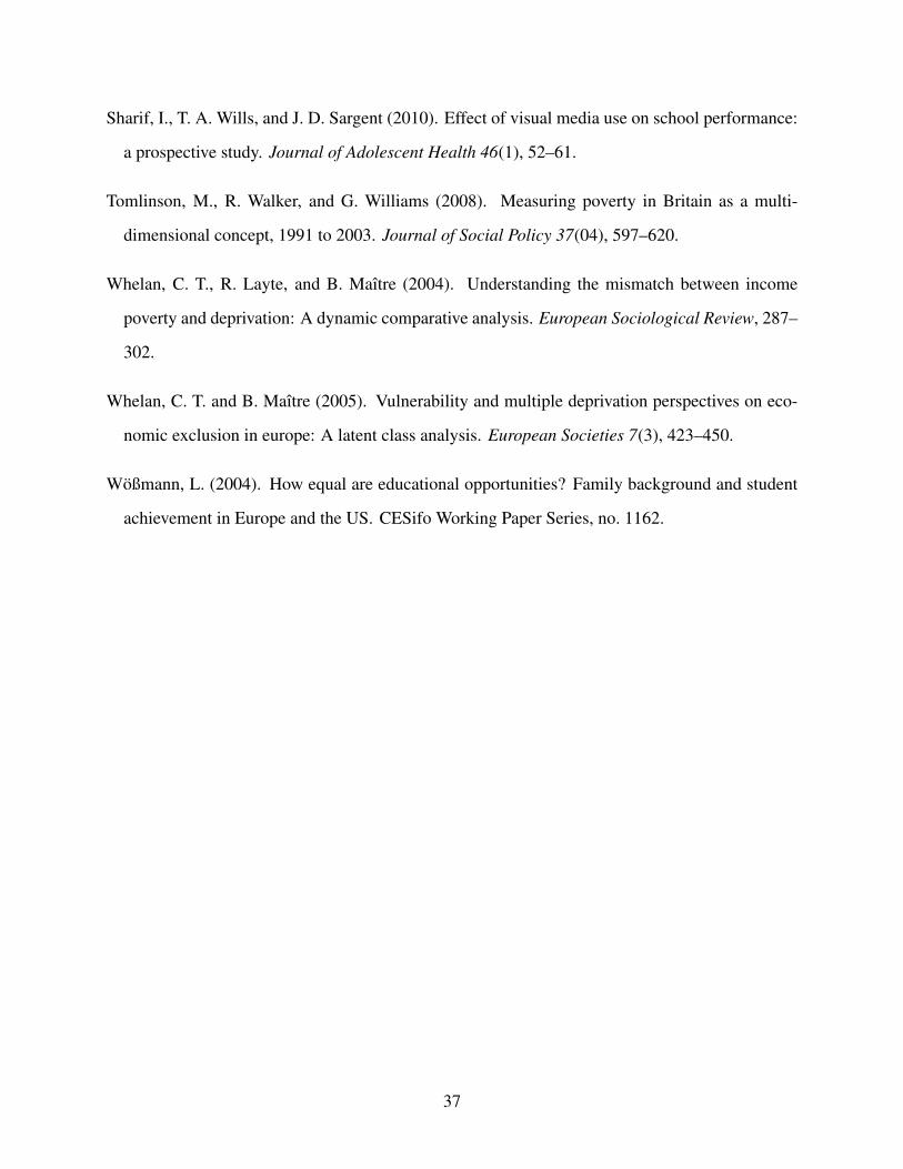
Sharif, I., T. A. Wills, and J. D. Sargent (2010). Effect of visual media use on school performance:

a prospective study. Journal of Adolescent Health 46(1), 52–61.

Tomlinson, M., R. Walker, and G. Williams (2008). Measuring poverty in Britain as a multi-

dimensional concept, 1991 to 2003. Journal of Social Policy 37(04), 597–620.

Whelan, C. T., R. Layte, and B. Maıtre (2004). Understanding the mismatch between income

poverty and deprivation: A dynamic comparative analysis. European Sociological Review, 287–

302.

Whelan, C. T. and B. Maıtre (2005). Vulnerability and multiple deprivation perspectives on eco-

nomic exclusion in europe: A latent class analysis. European Societies 7(3), 423–450.

Woßmann, L. (2004). How equal are educational opportunities? Family background and student

achievement in Europe and the US. CESifo Working Paper Series, no. 1162.

37

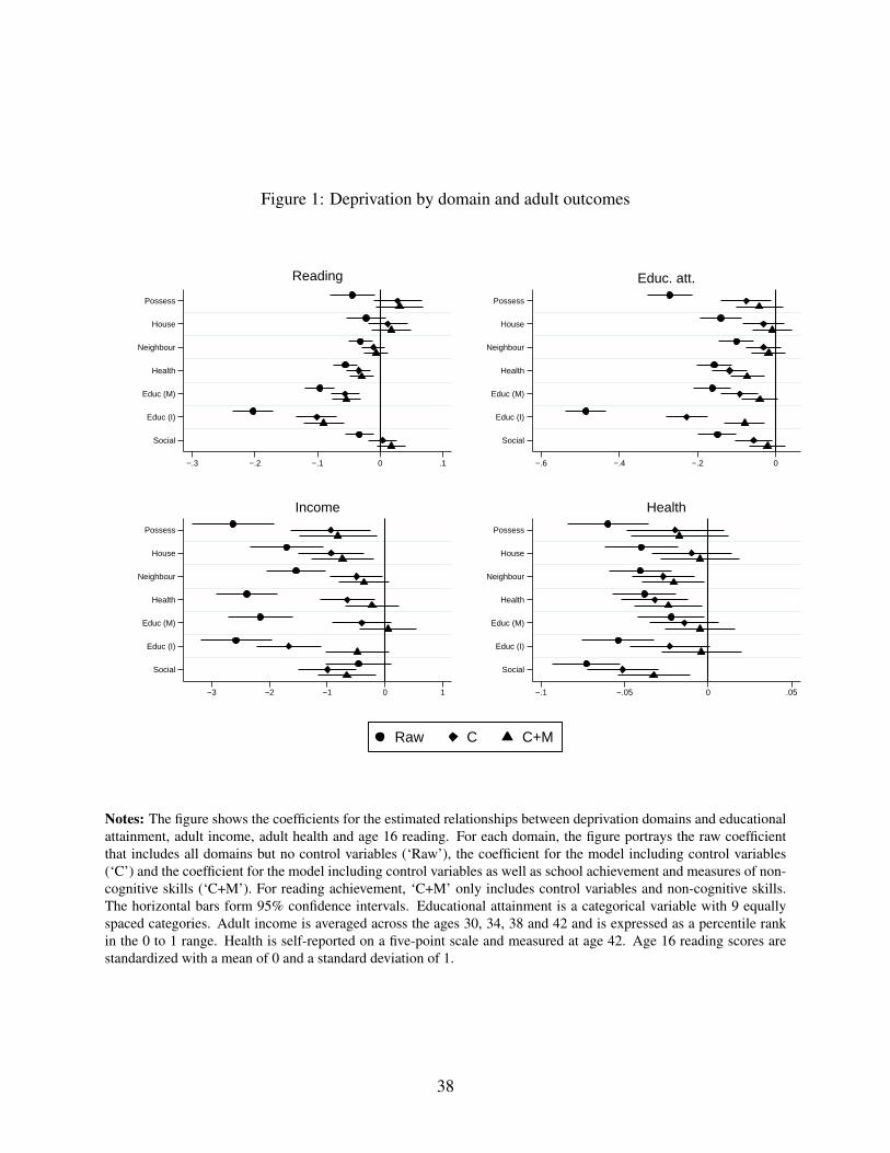
Figure 1: Deprivation by domain and adult outcomes

Possess

House

Neighbour

Health

Educ (M)

Educ (I)

Social

−.3 −.2 −.1 0 .1

Reading

Possess

House

Neighbour

Health

Educ (M)

Educ (I)

Social

−.6 −.4 −.2 0

Educ. att.

Possess

House

Neighbour

Health

Educ (M)

Educ (I)

Social

−3 −2 −1 0 1

Income

Possess

House

Neighbour

Health

Educ (M)

Educ (I)

Social

−.1 −.05 0 .05

Health

Raw C C+M

Notes: The figure shows the coefficients for the estimated relationships between deprivation domains and educationalattainment, adult income, adult health and age 16 reading. For each domain, the figure portrays the raw coefficientthat includes all domains but no control variables (‘Raw’), the coefficient for the model including control variables(‘C’) and the coefficient for the model including control variables as well as school achievement and measures of non-cognitive skills (‘C+M’). For reading achievement, ‘C+M’ only includes control variables and non-cognitive skills.The horizontal bars form 95% confidence intervals. Educational attainment is a categorical variable with 9 equallyspaced categories. Adult income is averaged across the ages 30, 34, 38 and 42 and is expressed as a percentile rankin the 0 to 1 range. Health is self-reported on a five-point scale and measured at age 42. Age 16 reading scores arestandardized with a mean of 0 and a standard deviation of 1.

38

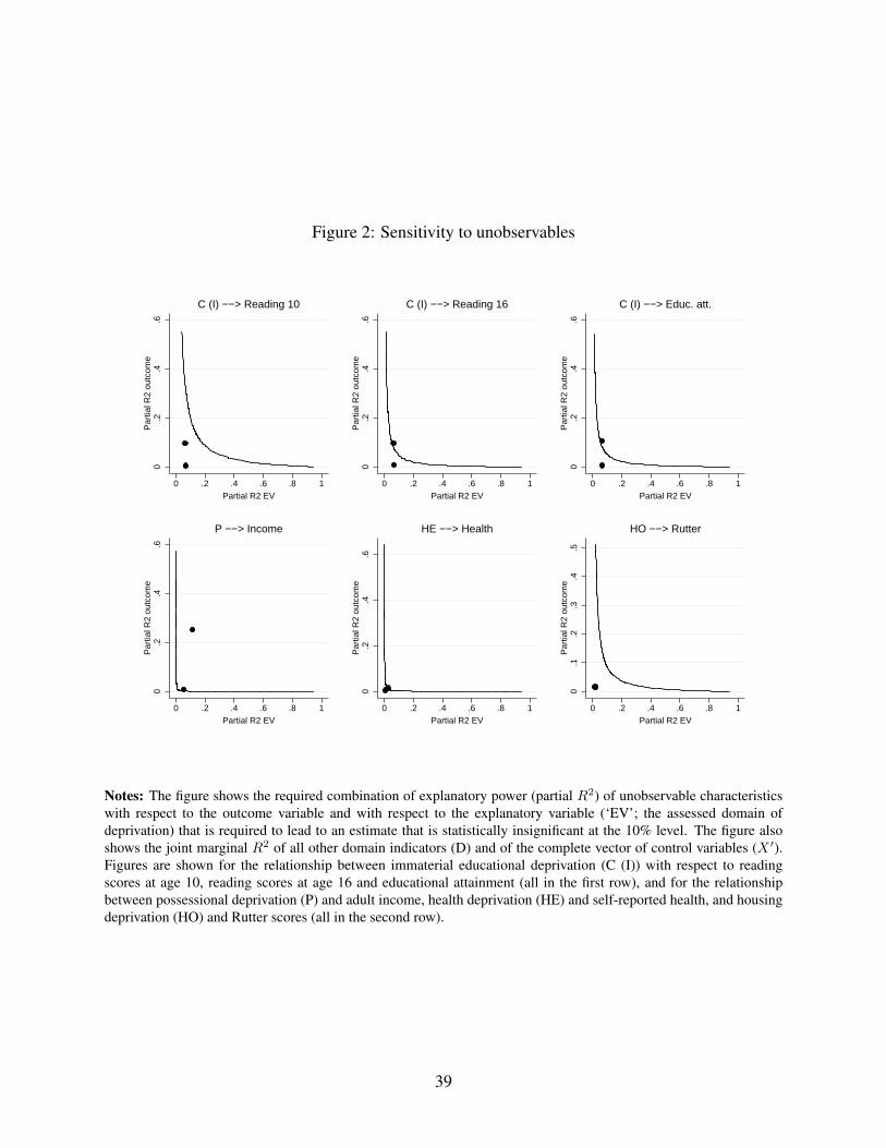
Figure 2: Sensitivity to unobservables

0.2

.4.6

Par

tial R

2 ou

tcom

e

0 .2 .4 .6 .8 1Partial R2 EV

C (I) −−> Reading 10

0.2

.4.6

Par

tial R

2 ou

tcom

e

0 .2 .4 .6 .8 1Partial R2 EV

C (I) −−> Reading 16

0.2

.4.6

Par

tial R

2 ou

tcom

e

0 .2 .4 .6 .8 1Partial R2 EV

C (I) −−> Educ. att.

0.2

.4.6

Par

tial R

2 ou

tcom

e

0 .2 .4 .6 .8 1Partial R2 EV

P −−> Income

0.2

.4.6

Par

tial R

2 ou

tcom

e

0 .2 .4 .6 .8 1Partial R2 EV

HE −−> Health

0.1

.2.3

.4.5

Par

tial R

2 ou

tcom

e

0 .2 .4 .6 .8 1Partial R2 EV

HO −−> Rutter

Notes: The figure shows the required combination of explanatory power (partial R2) of unobservable characteristicswith respect to the outcome variable and with respect to the explanatory variable (‘EV’; the assessed domain ofdeprivation) that is required to lead to an estimate that is statistically insignificant at the 10% level. The figure alsoshows the joint marginal R2 of all other domain indicators (D) and of the complete vector of control variables (X ′).Figures are shown for the relationship between immaterial educational deprivation (C (I)) with respect to readingscores at age 10, reading scores at age 16 and educational attainment (all in the first row), and for the relationshipbetween possessional deprivation (P) and adult income, health deprivation (HE) and self-reported health, and housingdeprivation (HO) and Rutter scores (all in the second row).

39

Figure 3: Explanatory variance across outcomes: deprivation versus background controls

Reading 16 Educ. att. Income

Health Math 16 Rutter 16

Self−esteem 16 Mental health Life satisfaction

Controls Domains

Notes: The figure shows the relative explanatory variance of background control variables (vector X ′ in Model 1) anddeprivation domains. The explanatory variance of the control variables is based on the R2 of a model regressing theoutcome only on the set of controls. The explanatory variance of the domains is based on the marginal addition to theR2 from further including deprivation domains.

40

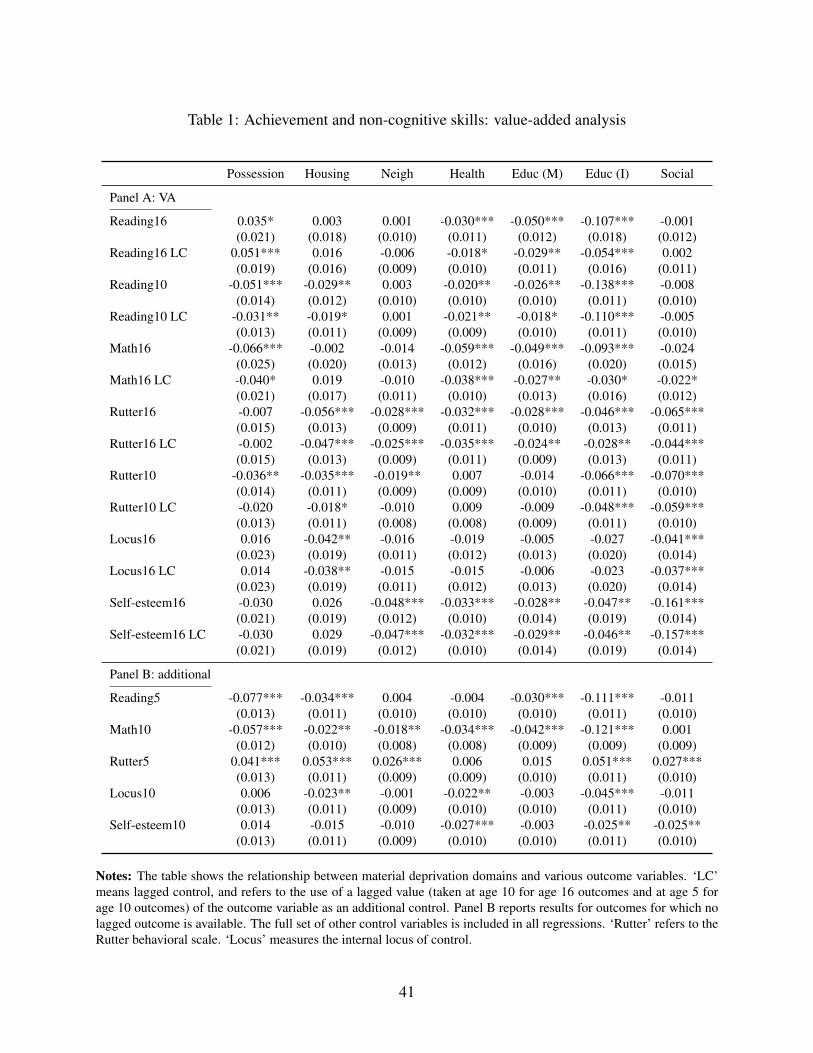
Table 1: Achievement and non-cognitive skills: value-added analysis

Possession Housing Neigh Health Educ (M) Educ (I) Social

Panel A: VA

Reading16 0.035* 0.003 0.001 -0.030*** -0.050*** -0.107*** -0.001(0.021) (0.018) (0.010) (0.011) (0.012) (0.018) (0.012)

Reading16 LC 0.051*** 0.016 -0.006 -0.018* -0.029** -0.054*** 0.002(0.019) (0.016) (0.009) (0.010) (0.011) (0.016) (0.011)

Reading10 -0.051*** -0.029** 0.003 -0.020** -0.026** -0.138*** -0.008(0.014) (0.012) (0.010) (0.010) (0.010) (0.011) (0.010)

Reading10 LC -0.031** -0.019* 0.001 -0.021** -0.018* -0.110*** -0.005(0.013) (0.011) (0.009) (0.009) (0.010) (0.011) (0.010)

Math16 -0.066*** -0.002 -0.014 -0.059*** -0.049*** -0.093*** -0.024(0.025) (0.020) (0.013) (0.012) (0.016) (0.020) (0.015)

Math16 LC -0.040* 0.019 -0.010 -0.038*** -0.027** -0.030* -0.022*(0.021) (0.017) (0.011) (0.010) (0.013) (0.016) (0.012)

Rutter16 -0.007 -0.056*** -0.028*** -0.032*** -0.028*** -0.046*** -0.065***(0.015) (0.013) (0.009) (0.011) (0.010) (0.013) (0.011)

Rutter16 LC -0.002 -0.047*** -0.025*** -0.035*** -0.024** -0.028** -0.044***(0.015) (0.013) (0.009) (0.011) (0.009) (0.013) (0.011)

Rutter10 -0.036** -0.035*** -0.019** 0.007 -0.014 -0.066*** -0.070***(0.014) (0.011) (0.009) (0.009) (0.010) (0.011) (0.010)

Rutter10 LC -0.020 -0.018* -0.010 0.009 -0.009 -0.048*** -0.059***(0.013) (0.011) (0.008) (0.008) (0.009) (0.011) (0.010)

Locus16 0.016 -0.042** -0.016 -0.019 -0.005 -0.027 -0.041***(0.023) (0.019) (0.011) (0.012) (0.013) (0.020) (0.014)

Locus16 LC 0.014 -0.038** -0.015 -0.015 -0.006 -0.023 -0.037***(0.023) (0.019) (0.011) (0.012) (0.013) (0.020) (0.014)

Self-esteem16 -0.030 0.026 -0.048*** -0.033*** -0.028** -0.047** -0.161***(0.021) (0.019) (0.012) (0.010) (0.014) (0.019) (0.014)

Self-esteem16 LC -0.030 0.029 -0.047*** -0.032*** -0.029** -0.046** -0.157***(0.021) (0.019) (0.012) (0.010) (0.014) (0.019) (0.014)

Panel B: additional

Reading5 -0.077*** -0.034*** 0.004 -0.004 -0.030*** -0.111*** -0.011(0.013) (0.011) (0.010) (0.010) (0.010) (0.011) (0.010)

Math10 -0.057*** -0.022** -0.018** -0.034*** -0.042*** -0.121*** 0.001(0.012) (0.010) (0.008) (0.008) (0.009) (0.009) (0.009)

Rutter5 0.041*** 0.053*** 0.026*** 0.006 0.015 0.051*** 0.027***(0.013) (0.011) (0.009) (0.009) (0.010) (0.011) (0.010)

Locus10 0.006 -0.023** -0.001 -0.022** -0.003 -0.045*** -0.011(0.013) (0.011) (0.009) (0.010) (0.010) (0.011) (0.010)

Self-esteem10 0.014 -0.015 -0.010 -0.027*** -0.003 -0.025** -0.025**(0.013) (0.011) (0.009) (0.010) (0.010) (0.011) (0.010)

Notes: The table shows the relationship between material deprivation domains and various outcome variables. ‘LC’means lagged control, and refers to the use of a lagged value (taken at age 10 for age 16 outcomes and at age 5 forage 10 outcomes) of the outcome variable as an additional control. Panel B reports results for outcomes for which nolagged outcome is available. The full set of other control variables is included in all regressions. ‘Rutter’ refers to theRutter behavioral scale. ‘Locus’ measures the internal locus of control.

41

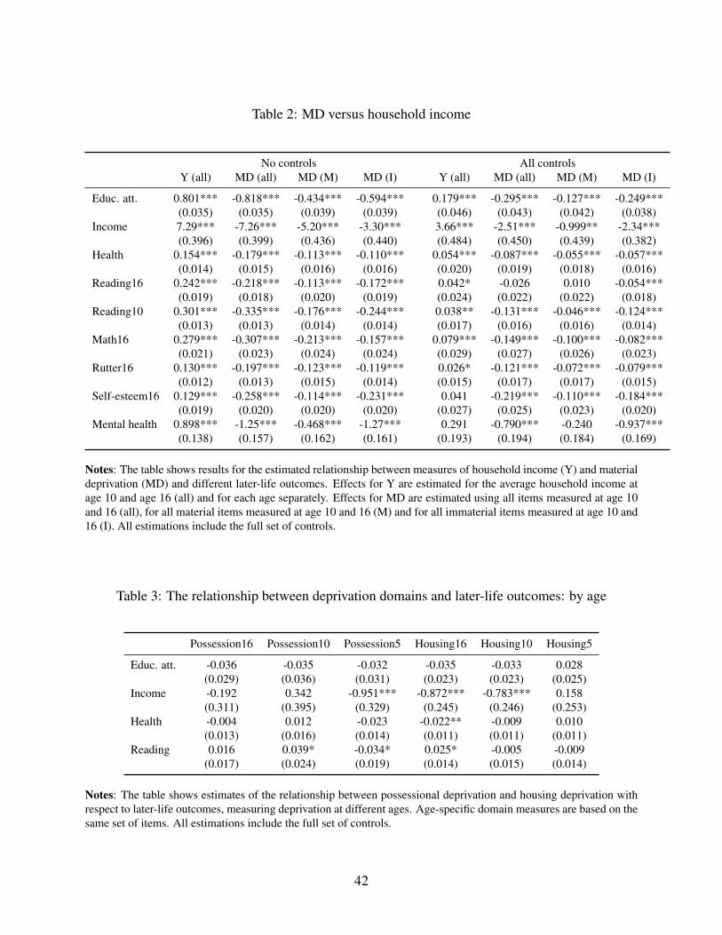
Table 2: MD versus household income

No controls All controlsY (all) MD (all) MD (M) MD (I) Y (all) MD (all) MD (M) MD (I)

Educ. att. 0.801*** -0.818*** -0.434*** -0.594*** 0.179*** -0.295*** -0.127*** -0.249***(0.035) (0.035) (0.039) (0.039) (0.046) (0.043) (0.042) (0.038)

Income 7.29*** -7.26*** -5.20*** -3.30*** 3.66*** -2.51*** -0.999** -2.34***(0.396) (0.399) (0.436) (0.440) (0.484) (0.450) (0.439) (0.382)

Health 0.154*** -0.179*** -0.113*** -0.110*** 0.054*** -0.087*** -0.055*** -0.057***(0.014) (0.015) (0.016) (0.016) (0.020) (0.019) (0.018) (0.016)

Reading16 0.242*** -0.218*** -0.113*** -0.172*** 0.042* -0.026 0.010 -0.054***(0.019) (0.018) (0.020) (0.019) (0.024) (0.022) (0.022) (0.018)

Reading10 0.301*** -0.335*** -0.176*** -0.244*** 0.038** -0.131*** -0.046*** -0.124***(0.013) (0.013) (0.014) (0.014) (0.017) (0.016) (0.016) (0.014)

Math16 0.279*** -0.307*** -0.213*** -0.157*** 0.079*** -0.149*** -0.100*** -0.082***(0.021) (0.023) (0.024) (0.024) (0.029) (0.027) (0.026) (0.023)

Rutter16 0.130*** -0.197*** -0.123*** -0.119*** 0.026* -0.121*** -0.072*** -0.079***(0.012) (0.013) (0.015) (0.014) (0.015) (0.017) (0.017) (0.015)

Self-esteem16 0.129*** -0.258*** -0.114*** -0.231*** 0.041 -0.219*** -0.110*** -0.184***(0.019) (0.020) (0.020) (0.020) (0.027) (0.025) (0.023) (0.020)

Mental health 0.898*** -1.25*** -0.468*** -1.27*** 0.291 -0.790*** -0.240 -0.937***(0.138) (0.157) (0.162) (0.161) (0.193) (0.194) (0.184) (0.169)

Notes: The table shows results for the estimated relationship between measures of household income (Y) and materialdeprivation (MD) and different later-life outcomes. Effects for Y are estimated for the average household income atage 10 and age 16 (all) and for each age separately. Effects for MD are estimated using all items measured at age 10and 16 (all), for all material items measured at age 10 and 16 (M) and for all immaterial items measured at age 10 and16 (I). All estimations include the full set of controls.

Table 3: The relationship between deprivation domains and later-life outcomes: by age

Possession16 Possession10 Possession5 Housing16 Housing10 Housing5

Educ. att. -0.036 -0.035 -0.032 -0.035 -0.033 0.028(0.029) (0.036) (0.031) (0.023) (0.023) (0.025)

Income -0.192 0.342 -0.951*** -0.872*** -0.783*** 0.158(0.311) (0.395) (0.329) (0.245) (0.246) (0.253)

Health -0.004 0.012 -0.023 -0.022** -0.009 0.010(0.013) (0.016) (0.014) (0.011) (0.011) (0.011)

Reading 0.016 0.039* -0.034* 0.025* -0.005 -0.009(0.017) (0.024) (0.019) (0.014) (0.015) (0.014)

Notes: The table shows estimates of the relationship between possessional deprivation and housing deprivation withrespect to later-life outcomes, measuring deprivation at different ages. Age-specific domain measures are based on thesame set of items. All estimations include the full set of controls.

42

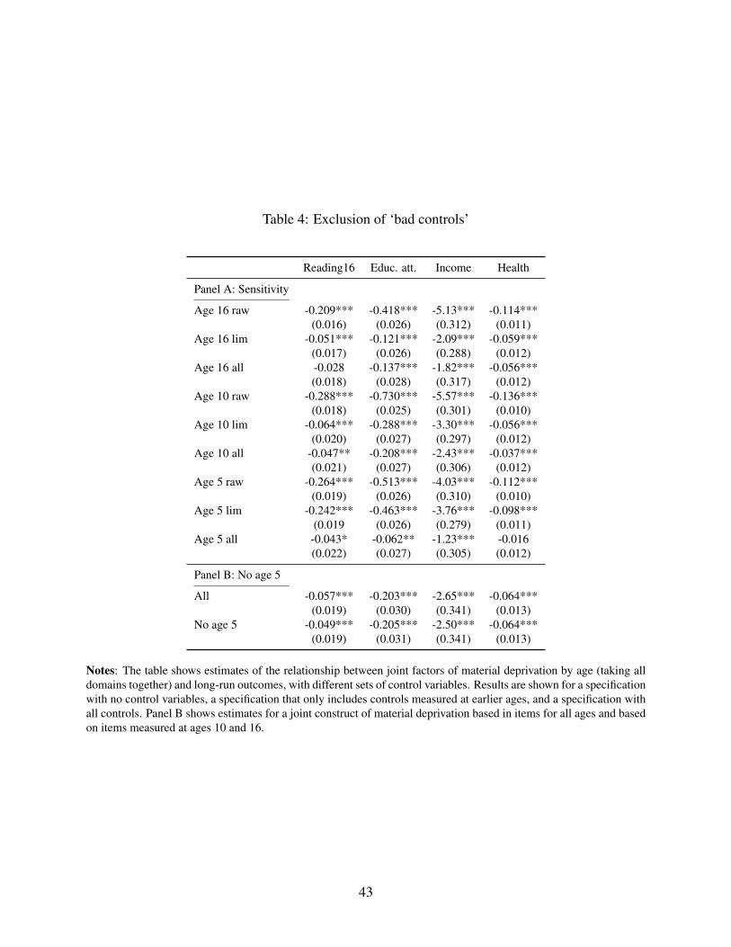
Table 4: Exclusion of ‘bad controls’

Reading16 Educ. att. Income Health

Panel A: Sensitivity

Age 16 raw -0.209*** -0.418*** -5.13*** -0.114***(0.016) (0.026) (0.312) (0.011)

Age 16 lim -0.051*** -0.121*** -2.09*** -0.059***(0.017) (0.026) (0.288) (0.012)

Age 16 all -0.028 -0.137*** -1.82*** -0.056***(0.018) (0.028) (0.317) (0.012)

Age 10 raw -0.288*** -0.730*** -5.57*** -0.136***(0.018) (0.025) (0.301) (0.010)

Age 10 lim -0.064*** -0.288*** -3.30*** -0.056***(0.020) (0.027) (0.297) (0.012)

Age 10 all -0.047** -0.208*** -2.43*** -0.037***(0.021) (0.027) (0.306) (0.012)

Age 5 raw -0.264*** -0.513*** -4.03*** -0.112***(0.019) (0.026) (0.310) (0.010)

Age 5 lim -0.242*** -0.463*** -3.76*** -0.098***(0.019 (0.026) (0.279) (0.011)

Age 5 all -0.043* -0.062** -1.23*** -0.016(0.022) (0.027) (0.305) (0.012)

Panel B: No age 5

All -0.057*** -0.203*** -2.65*** -0.064***(0.019) (0.030) (0.341) (0.013)

No age 5 -0.049*** -0.205*** -2.50*** -0.064***(0.019) (0.031) (0.341) (0.013)

Notes: The table shows estimates of the relationship between joint factors of material deprivation by age (taking alldomains together) and long-run outcomes, with different sets of control variables. Results are shown for a specificationwith no control variables, a specification that only includes controls measured at earlier ages, and a specification withall controls. Panel B shows estimates for a joint construct of material deprivation based in items for all ages and basedon items measured at ages 10 and 16.

43

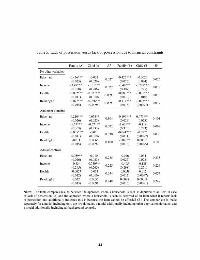
Table 5: Lack of possession versus lack of possession due to financial constraints

Family (A) Child (A) R2 Family (B) Child (B) R2

No other variables

Educ. att. -0.426*** -0.032 0.027 -0.423*** -0.0024 0.025(0.025) (0.026) (0.026) (0.024)Income -3.49*** -1.31*** 0.022 -3.48*** -0.729*** 0.018(0.288) (0.286) (0.307) (0.275)Health -0.082*** -0.037*** 0.0093 -0.089*** -0.035*** 0.010(0.011) (0.010) (0.010) (0.010)Reading16 -0.077*** -0.026*** 0.0093 -0.114*** -0.027*** 0.017(0.015) (0.0098) (0.016) (0.0097)

Add other domains

Educ. att. -0.210*** 0.054** 0.104 -0.196*** 0.075*** 0.101(0.026) (0.025) (0.029) (0.025)Income -1.77*** -0.574** 0.072 -1.63*** -0.118 0.069(0.303) (0.283) (0.310) (0.273)Health -0.035*** -0.015 0.030 -0.041*** -0.017* 0.030(0.011) (0.010) (0.011) (0.0097)Reading16 -0.011 0.0065 0.100 -0.040** 0.00011 0.100(0.015) (0.0097) (0.016) (0.0095)

Add all controls

Educ. att. -0.059** 0.010 0.235 -0.026 0.034 0.235(0.026) (0.023) (0.027) (0.023)Income -0.434 -0.740*** 0.225 -0.405 -0.188 0.224(0.295) (0.265) (0.298) (0.251)Health -0.0027 -0.013 0.054 -0.0058 -0.015 0.053(0.012) (0.010) (0.012) (0.0097)Reading16 0.022 0.0055 0.248 0.0098 0.00018 0.248(0.015) (0.0091) (0.016) (0.0091)

Notes: The table compares results between the approach where a household is seen as deprived of an item in caseof lack of possession (A) and the approach where a household is seen as deprived of an item when it reports lackof possession and additionally indicates this is because the item cannot be afforded (B). The comparison is madeseparately for a model including only the two domains, a model additionally including other deprivation domains, anda model additionally including all background controls.

44

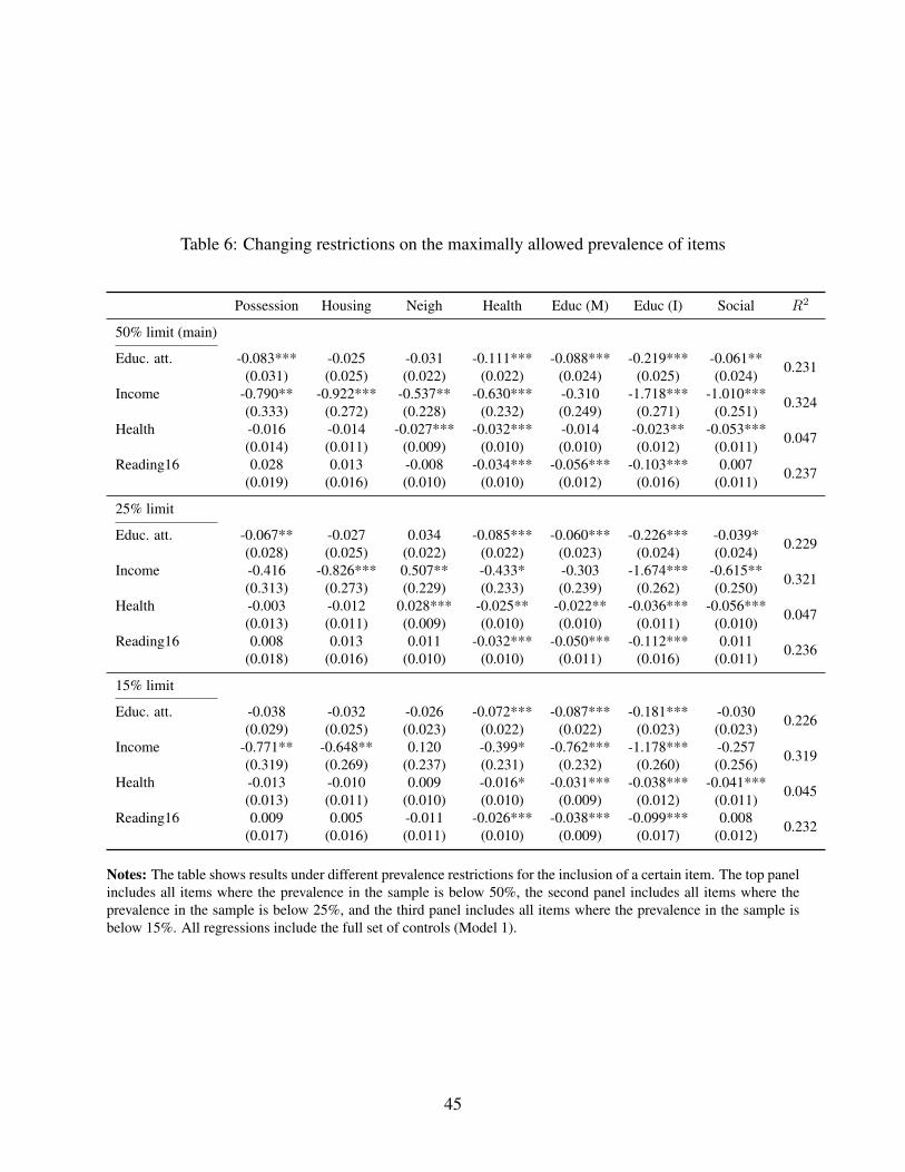
Table 6: Changing restrictions on the maximally allowed prevalence of items

Possession Housing Neigh Health Educ (M) Educ (I) Social R2

50% limit (main)

Educ. att. -0.083*** -0.025 -0.031 -0.111*** -0.088*** -0.219*** -0.061** 0.231(0.031) (0.025) (0.022) (0.022) (0.024) (0.025) (0.024)Income -0.790** -0.922*** -0.537** -0.630*** -0.310 -1.718*** -1.010*** 0.324(0.333) (0.272) (0.228) (0.232) (0.249) (0.271) (0.251)Health -0.016 -0.014 -0.027*** -0.032*** -0.014 -0.023** -0.053*** 0.047(0.014) (0.011) (0.009) (0.010) (0.010) (0.012) (0.011)Reading16 0.028 0.013 -0.008 -0.034*** -0.056*** -0.103*** 0.007 0.237(0.019) (0.016) (0.010) (0.010) (0.012) (0.016) (0.011)

25% limit

Educ. att. -0.067** -0.027 0.034 -0.085*** -0.060*** -0.226*** -0.039* 0.229(0.028) (0.025) (0.022) (0.022) (0.023) (0.024) (0.024)Income -0.416 -0.826*** 0.507** -0.433* -0.303 -1.674*** -0.615** 0.321(0.313) (0.273) (0.229) (0.233) (0.239) (0.262) (0.250)Health -0.003 -0.012 0.028*** -0.025** -0.022** -0.036*** -0.056*** 0.047(0.013) (0.011) (0.009) (0.010) (0.010) (0.011) (0.010)Reading16 0.008 0.013 0.011 -0.032*** -0.050*** -0.112*** 0.011 0.236(0.018) (0.016) (0.010) (0.010) (0.011) (0.016) (0.011)

15% limit

Educ. att. -0.038 -0.032 -0.026 -0.072*** -0.087*** -0.181*** -0.030 0.226(0.029) (0.025) (0.023) (0.022) (0.022) (0.023) (0.023)Income -0.771** -0.648** 0.120 -0.399* -0.762*** -1.178*** -0.257 0.319(0.319) (0.269) (0.237) (0.231) (0.232) (0.260) (0.256)Health -0.013 -0.010 0.009 -0.016* -0.031*** -0.038*** -0.041*** 0.045(0.013) (0.011) (0.010) (0.010) (0.009) (0.012) (0.011)Reading16 0.009 0.005 -0.011 -0.026*** -0.038*** -0.099*** 0.008 0.232(0.017) (0.016) (0.011) (0.010) (0.009) (0.017) (0.012)

Notes: The table shows results under different prevalence restrictions for the inclusion of a certain item. The top panelincludes all items where the prevalence in the sample is below 50%, the second panel includes all items where theprevalence in the sample is below 25%, and the third panel includes all items where the prevalence in the sample isbelow 15%. All regressions include the full set of controls (Model 1).

45

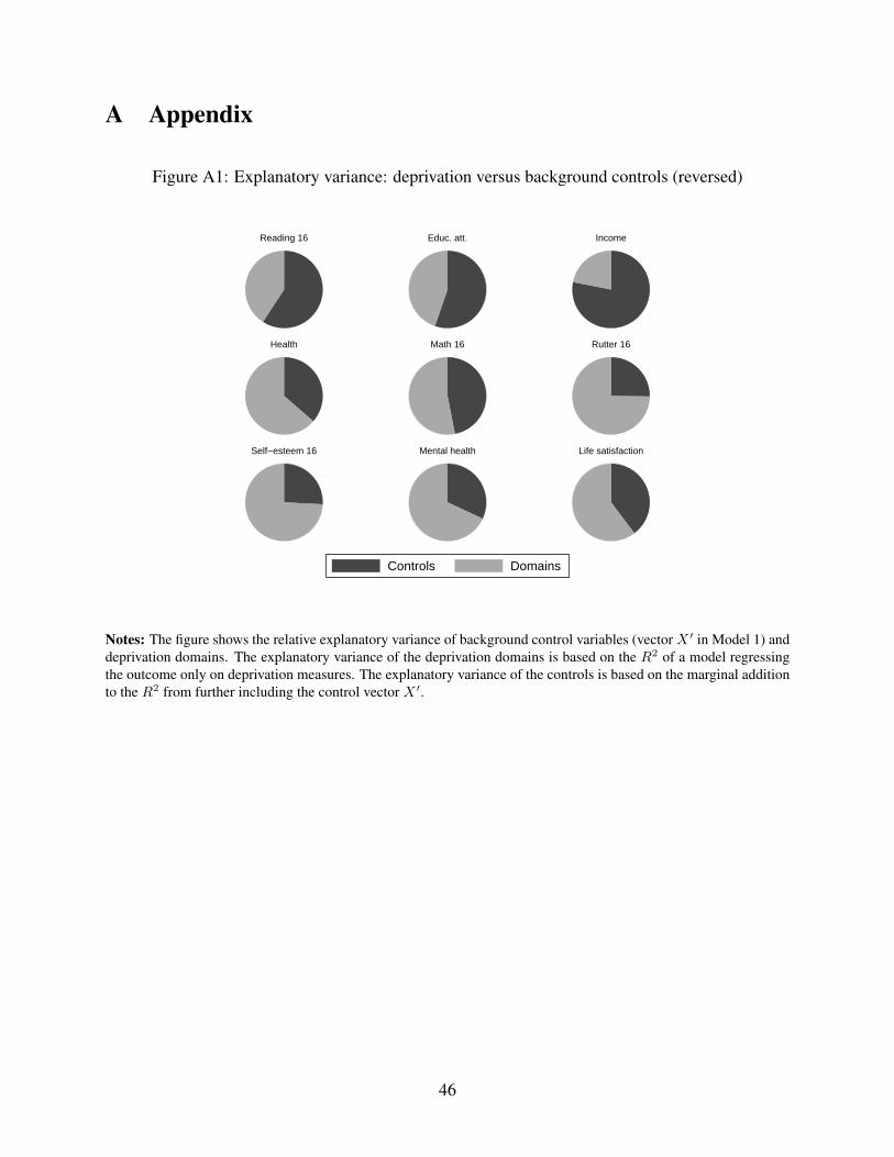
A Appendix

Figure A1: Explanatory variance: deprivation versus background controls (reversed)

Reading 16 Educ. att. Income

Health Math 16 Rutter 16

Self−esteem 16 Mental health Life satisfaction

Controls Domains

Notes: The figure shows the relative explanatory variance of background control variables (vector X ′ in Model 1) anddeprivation domains. The explanatory variance of the deprivation domains is based on the R2 of a model regressingthe outcome only on deprivation measures. The explanatory variance of the controls is based on the marginal additionto the R2 from further including the control vector X ′.

46

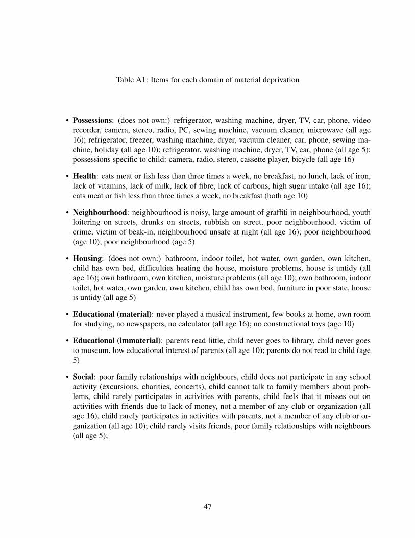
Table A1: Items for each domain of material deprivation

• Possessions: (does not own:) refrigerator, washing machine, dryer, TV, car, phone, videorecorder, camera, stereo, radio, PC, sewing machine, vacuum cleaner, microwave (all age16); refrigerator, freezer, washing machine, dryer, vacuum cleaner, car, phone, sewing ma-chine, holiday (all age 10); refrigerator, washing machine, dryer, TV, car, phone (all age 5);possessions specific to child: camera, radio, stereo, cassette player, bicycle (all age 16)

• Health: eats meat or fish less than three times a week, no breakfast, no lunch, lack of iron,lack of vitamins, lack of milk, lack of fibre, lack of carbons, high sugar intake (all age 16);eats meat or fish less than three times a week, no breakfast (both age 10)

• Neighbourhood: neighbourhood is noisy, large amount of graffiti in neighbourhood, youthloitering on streets, drunks on streets, rubbish on street, poor neighbourhood, victim ofcrime, victim of beak-in, neighbourhood unsafe at night (all age 16); poor neighbourhood(age 10); poor neighbourhood (age 5)

• Housing: (does not own:) bathroom, indoor toilet, hot water, own garden, own kitchen,child has own bed, difficulties heating the house, moisture problems, house is untidy (allage 16); own bathroom, own kitchen, moisture problems (all age 10); own bathroom, indoortoilet, hot water, own garden, own kitchen, child has own bed, furniture in poor state, houseis untidy (all age 5)

• Educational (material): never played a musical instrument, few books at home, own roomfor studying, no newspapers, no calculator (all age 16); no constructional toys (age 10)

• Educational (immaterial): parents read little, child never goes to library, child never goesto museum, low educational interest of parents (all age 10); parents do not read to child (age5)

• Social: poor family relationships with neighbours, child does not participate in any schoolactivity (excursions, charities, concerts), child cannot talk to family members about prob-lems, child rarely participates in activities with parents, child feels that it misses out onactivities with friends due to lack of money, not a member of any club or organization (allage 16), child rarely participates in activities with parents, not a member of any club or or-ganization (all age 10); child rarely visits friends, poor family relationships with neighbours(all age 5);

47

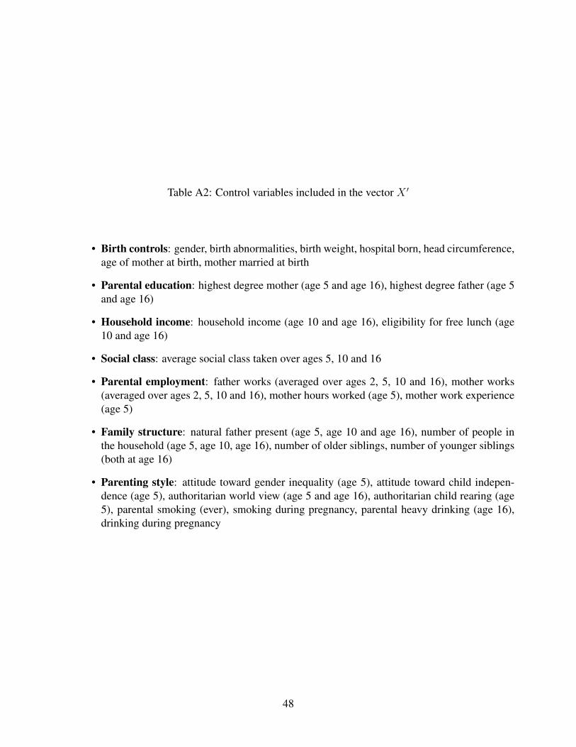
Table A2: Control variables included in the vector X ′

• Birth controls: gender, birth abnormalities, birth weight, hospital born, head circumference,age of mother at birth, mother married at birth

• Parental education: highest degree mother (age 5 and age 16), highest degree father (age 5and age 16)

• Household income: household income (age 10 and age 16), eligibility for free lunch (age10 and age 16)

• Social class: average social class taken over ages 5, 10 and 16

• Parental employment: father works (averaged over ages 2, 5, 10 and 16), mother works(averaged over ages 2, 5, 10 and 16), mother hours worked (age 5), mother work experience(age 5)

• Family structure: natural father present (age 5, age 10 and age 16), number of people inthe household (age 5, age 10, age 16), number of older siblings, number of younger siblings(both at age 16)

• Parenting style: attitude toward gender inequality (age 5), attitude toward child indepen-dence (age 5), authoritarian world view (age 5 and age 16), authoritarian child rearing (age5), parental smoking (ever), smoking during pregnancy, parental heavy drinking (age 16),drinking during pregnancy

48

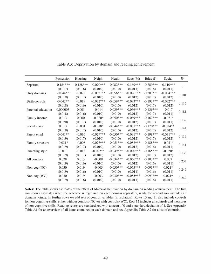
Table A3: Deprivation by domain and reading achievement

Possession Housing Neigh Health Educ (M) Educ (I) Social R2

Separate -0.184*** -0.128*** -0.070*** -0.082*** -0.169*** -0.289*** -0.110*** -(0.017) (0.016) (0.010) (0.010) (0.011) (0.016) (0.011)Only domains -0.044** -0.023 -0.032*** -0.056*** -0.096*** -0.203*** -0.034*** 0.101(0.019) (0.017) (0.010) (0.010) (0.012) (0.017) (0.012)Birth controls -0.042** -0.019 -0.032*** -0.059*** -0.093*** -0.193*** -0.032*** 0.115(0.018) (0.016) (0.010) (0.010) (0.012) (0.017) (0.012)Parental education 0.000003 0.001 -0.014 -0.039*** -0.066*** -0.136*** -0.017 0.181(0.018) (0.016) (0.010) (0.010) (0.012) (0.017) (0.011)Family income 0.013 0.000 -0.020* -0.050*** -0.089*** -0.167*** -0.021* 0.132(0.020) (0.017) (0.010) (0.010) (0.012) (0.017) (0.011)Social class 0.013 -0.001 -0.018* -0.044*** -0.081*** -0.170*** -0.024** 0.144(0.019) (0.017) (0.010) (0.010) (0.012) (0.017) (0.012)Parent empl -0.041** -0.016 -0.029*** -0.050*** -0.091*** -0.198*** -0.031*** 0.119(0.019) (0.017) (0.010) (0.010) (0.012) (0.017) (0.012)Family structure -0.031* -0.008 -0.027*** -0.051*** -0.088*** -0.188*** -0.021* 0.141(0.019) (0.017) (0.010) (0.010) (0.012) (0.016) (0.011)Parenting style -0.010 -0.013 -0.022** -0.049*** -0.090*** -0.165*** -0.020* 0.133(0.019) (0.017) (0.010) (0.010) (0.012) (0.017) (0.012)All controls 0.028 0.013 -0.008 -0.034*** -0.056*** -0.103*** 0.007 0.237(0.019) (0.016) (0.010) (0.010) (0.012) (0.016) (0.011)Non-cog (NC) 0.030 0.019 -0.003 -0.030*** -0.055*** -0.093*** 0.021* 0.249(0.019) (0.016) (0.010) (0.010) (0.011) (0.016) (0.011)Non-cog (WC) 0.030 0.019 -0.003 -0.030*** -0.055*** -0.093*** 0.021* 0.249(0.019) (0.016) (0.010) (0.010) (0.011) (0.016) (0.011)

Notes: The table shows estimates of the effect of Material Deprivation by domain on reading achievement. The firstrow shows estimates when the outcome is regressed on each domain separately, while the second row includes alldomains jointly. In further rows we add sets of control variables (in isolation). Rows 10 and 11 also include controlsfor non-cognitive skills, either without controls (NC) or with controls (WC). Row 12 includes all controls and measuresof non-cognitive skills. Reading scores are standardized with a mean of 0 and a standard deviation of 1. See AppendixTable A1 for an overview of all items contained in each domain and see Appendix Table A2 for a list of controls.

49

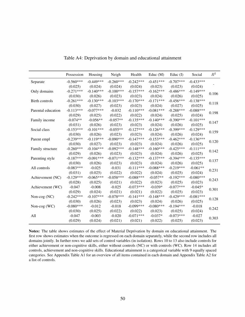
Table A4: Deprivation by domain and educational attainment

Possession Housing Neigh Health Educ (M) Educ (I) Social R2

Separate -0.560*** -0.449*** -0.260*** -0.242*** -0.451*** -0.707*** -0.433*** -(0.025) (0.024) (0.024) (0.024) (0.023) (0.023) (0.024)Only domains -0.271*** -0.140*** -0.100*** -0.157*** -0.162*** -0.486*** -0.149*** 0.106(0.030) (0.026) (0.023) (0.023) (0.024) (0.026) (0.025)Birth controls -0.261*** -0.130*** -0.103*** -0.170*** -0.171*** -0.456*** -0.138*** 0.118(0.030) (0.027) (0.023) (0.023) (0.024) (0.027) (0.025)Parental education -0.113*** -0.077*** -0.032 -0.110*** -0.081*** -0.288*** -0.088*** 0.198(0.029) (0.025) (0.022) (0.022) (0.024) (0.025) (0.024)Family income -0.074** -0.056** -0.057** -0.135*** -0.140*** -0.390*** -0.101*** 0.147(0.031) (0.026) (0.023) (0.023) (0.024) (0.026) (0.025)Social class -0.153*** -0.101*** -0.055** -0.127*** -0.126*** -0.399*** -0.129*** 0.159(0.030) (0.026) (0.023) (0.023) (0.024) (0.026) (0.024)Parent empl -0.239*** -0.119*** -0.090*** -0.147*** -0.153*** -0.462*** -0.136*** 0.120(0.030) (0.027) (0.023) (0.023) (0.024) (0.026) (0.025)Family structure -0.260*** -0.104*** -0.092*** -0.148*** -0.160*** -0.425*** -0.111*** 0.142(0.029) (0.026) (0.023) (0.023) (0.024) (0.026) (0.025)Parenting style -0.187*** -0.091*** -0.071*** -0.132*** -0.137*** -0.394*** -0.135*** 0.137(0.030) (0.026) (0.023) (0.023) (0.024) (0.026) (0.025)All controls -0.083*** -0.025 -0.031 -0.111*** -0.088*** -0.219*** -0.061** 0.231(0.031) (0.025) (0.022) (0.022) (0.024) (0.025) (0.024)Achievement (NC) -0.129*** -0.065*** -0.058*** -0.088*** -0.057** -0.192*** -0.080*** 0.243(0.028) (0.025) (0.021) (0.022) (0.023) (0.025) (0.023)Achievement (WC) -0.047 -0.008 -0.025 -0.073*** -0.039* -0.077*** -0.045* 0.301(0.029) (0.024) (0.021) (0.021) (0.022) (0.025) (0.023)Non-cog (NC) -0.242*** -0.107*** -0.078*** -0.141*** -0.148*** -0.429*** -0.081*** 0.128(0.030) (0.026) (0.023) (0.023) (0.024) (0.026) (0.025)Non-cog (WC) -0.080*** -0.012 -0.018 -0.099*** -0.080*** -0.194*** -0.018 0.242(0.030) (0.025) (0.022) (0.022) (0.023) (0.025) (0.024)All -0.047 -0.003 -0.020 -0.071*** -0.037* -0.073*** -0.027 0.303(0.029) (0.024) (0.021) (0.021) (0.022) (0.025) (0.023)

Notes: The table shows estimates of the effect of Material Deprivation by domain on educational attainment. Thefirst row shows estimates when the outcome is regressed on each domain separately, while the second row includes alldomains jointly. In further rows we add sets of control variables (in isolation). Rows 10 to 13 also include controls foreither achievement or non-cognitive skills, either without controls (NC) or with controls (WC). Row 14 includes allcontrols, achievement and non-cognitive skills. Educational attainment is a categorical variable with 9 equally spacedcategories. See Appendix Table A1 for an overview of all items contained in each domain and Appendix Table A2 fora list of controls.

50

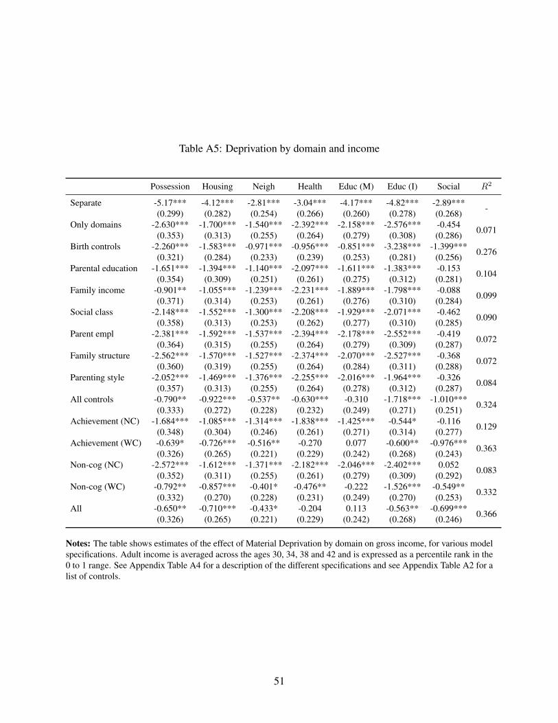
Table A5: Deprivation by domain and income

Possession Housing Neigh Health Educ (M) Educ (I) Social R2

Separate -5.17*** -4.12*** -2.81*** -3.04*** -4.17*** -4.82*** -2.89*** -(0.299) (0.282) (0.254) (0.266) (0.260) (0.278) (0.268)Only domains -2.630*** -1.700*** -1.540*** -2.392*** -2.158*** -2.576*** -0.454 0.071(0.353) (0.313) (0.255) (0.264) (0.279) (0.308) (0.286)Birth controls -2.260*** -1.583*** -0.971*** -0.956*** -0.851*** -3.238*** -1.399*** 0.276(0.321) (0.284) (0.233) (0.239) (0.253) (0.281) (0.256)Parental education -1.651*** -1.394*** -1.140*** -2.097*** -1.611*** -1.383*** -0.153 0.104(0.354) (0.309) (0.251) (0.261) (0.275) (0.312) (0.281)Family income -0.901** -1.055*** -1.239*** -2.231*** -1.889*** -1.798*** -0.088 0.099(0.371) (0.314) (0.253) (0.261) (0.276) (0.310) (0.284)Social class -2.148*** -1.552*** -1.300*** -2.208*** -1.929*** -2.071*** -0.462 0.090(0.358) (0.313) (0.253) (0.262) (0.277) (0.310) (0.285)Parent empl -2.381*** -1.592*** -1.537*** -2.394*** -2.178*** -2.552*** -0.419 0.072(0.364) (0.315) (0.255) (0.264) (0.279) (0.309) (0.287)Family structure -2.562*** -1.570*** -1.527*** -2.374*** -2.070*** -2.527*** -0.368 0.072(0.360) (0.319) (0.255) (0.264) (0.284) (0.311) (0.288)Parenting style -2.052*** -1.469*** -1.376*** -2.255*** -2.016*** -1.964*** -0.326 0.084(0.357) (0.313) (0.255) (0.264) (0.278) (0.312) (0.287)All controls -0.790** -0.922*** -0.537** -0.630*** -0.310 -1.718*** -1.010*** 0.324(0.333) (0.272) (0.228) (0.232) (0.249) (0.271) (0.251)Achievement (NC) -1.684*** -1.085*** -1.314*** -1.838*** -1.425*** -0.544* -0.116 0.129(0.348) (0.304) (0.246) (0.261) (0.271) (0.314) (0.277)Achievement (WC) -0.639* -0.726*** -0.516** -0.270 0.077 -0.600** -0.976*** 0.363(0.326) (0.265) (0.221) (0.229) (0.242) (0.268) (0.243)Non-cog (NC) -2.572*** -1.612*** -1.371*** -2.182*** -2.046*** -2.402*** 0.052 0.083(0.352) (0.311) (0.255) (0.261) (0.279) (0.309) (0.292)Non-cog (WC) -0.792** -0.857*** -0.401* -0.476** -0.222 -1.526*** -0.549** 0.332(0.332) (0.270) (0.228) (0.231) (0.249) (0.270) (0.253)All -0.650** -0.710*** -0.433* -0.204 0.113 -0.563** -0.699*** 0.366(0.326) (0.265) (0.221) (0.229) (0.242) (0.268) (0.246)

Notes: The table shows estimates of the effect of Material Deprivation by domain on gross income, for various modelspecifications. Adult income is averaged across the ages 30, 34, 38 and 42 and is expressed as a percentile rank in the0 to 1 range. See Appendix Table A4 for a description of the different specifications and see Appendix Table A2 for alist of controls.

51

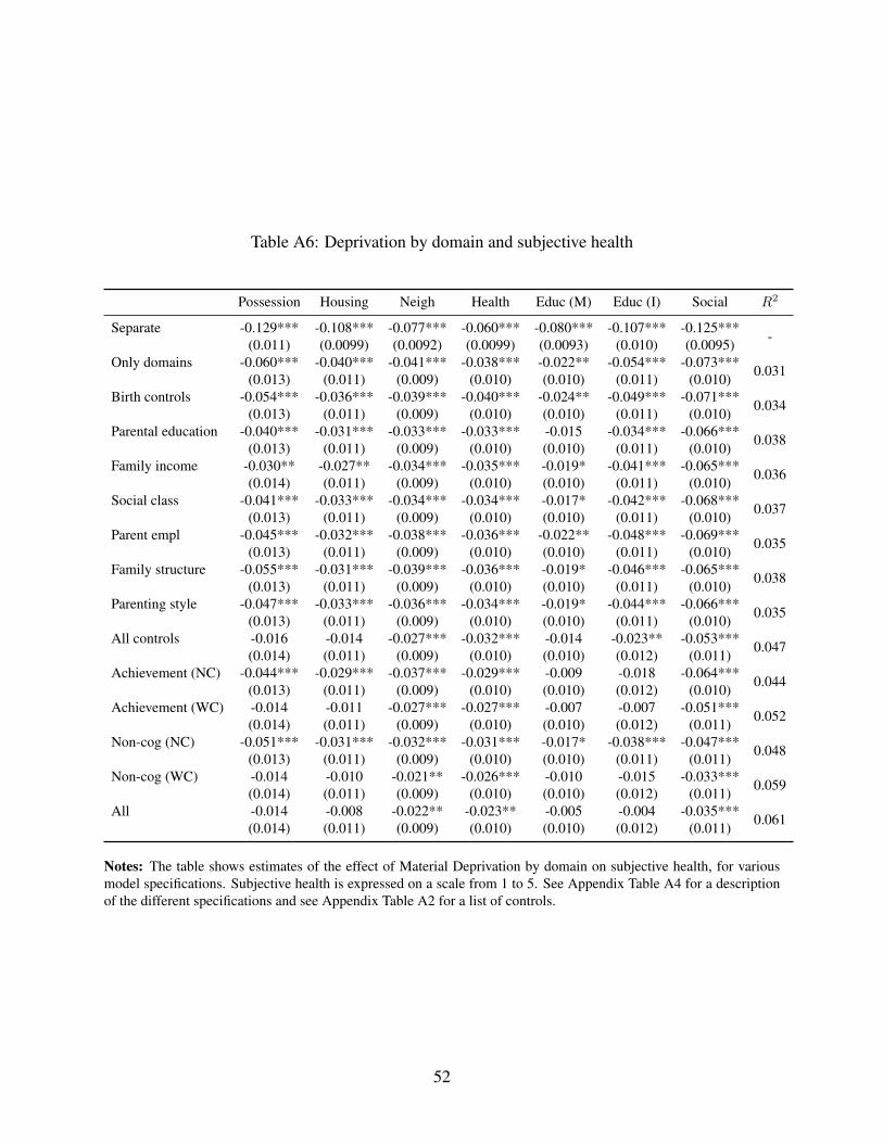
Table A6: Deprivation by domain and subjective health

Possession Housing Neigh Health Educ (M) Educ (I) Social R2

Separate -0.129*** -0.108*** -0.077*** -0.060*** -0.080*** -0.107*** -0.125*** -(0.011) (0.0099) (0.0092) (0.0099) (0.0093) (0.010) (0.0095)Only domains -0.060*** -0.040*** -0.041*** -0.038*** -0.022** -0.054*** -0.073*** 0.031(0.013) (0.011) (0.009) (0.010) (0.010) (0.011) (0.010)Birth controls -0.054*** -0.036*** -0.039*** -0.040*** -0.024** -0.049*** -0.071*** 0.034(0.013) (0.011) (0.009) (0.010) (0.010) (0.011) (0.010)Parental education -0.040*** -0.031*** -0.033*** -0.033*** -0.015 -0.034*** -0.066*** 0.038(0.013) (0.011) (0.009) (0.010) (0.010) (0.011) (0.010)Family income -0.030** -0.027** -0.034*** -0.035*** -0.019* -0.041*** -0.065*** 0.036(0.014) (0.011) (0.009) (0.010) (0.010) (0.011) (0.010)Social class -0.041*** -0.033*** -0.034*** -0.034*** -0.017* -0.042*** -0.068*** 0.037(0.013) (0.011) (0.009) (0.010) (0.010) (0.011) (0.010)Parent empl -0.045*** -0.032*** -0.038*** -0.036*** -0.022** -0.048*** -0.069*** 0.035(0.013) (0.011) (0.009) (0.010) (0.010) (0.011) (0.010)Family structure -0.055*** -0.031*** -0.039*** -0.036*** -0.019* -0.046*** -0.065*** 0.038(0.013) (0.011) (0.009) (0.010) (0.010) (0.011) (0.010)Parenting style -0.047*** -0.033*** -0.036*** -0.034*** -0.019* -0.044*** -0.066*** 0.035(0.013) (0.011) (0.009) (0.010) (0.010) (0.011) (0.010)All controls -0.016 -0.014 -0.027*** -0.032*** -0.014 -0.023** -0.053*** 0.047(0.014) (0.011) (0.009) (0.010) (0.010) (0.012) (0.011)Achievement (NC) -0.044*** -0.029*** -0.037*** -0.029*** -0.009 -0.018 -0.064*** 0.044(0.013) (0.011) (0.009) (0.010) (0.010) (0.012) (0.010)Achievement (WC) -0.014 -0.011 -0.027*** -0.027*** -0.007 -0.007 -0.051*** 0.052(0.014) (0.011) (0.009) (0.010) (0.010) (0.012) (0.011)Non-cog (NC) -0.051*** -0.031*** -0.032*** -0.031*** -0.017* -0.038*** -0.047*** 0.048(0.013) (0.011) (0.009) (0.010) (0.010) (0.011) (0.011)Non-cog (WC) -0.014 -0.010 -0.021** -0.026*** -0.010 -0.015 -0.033*** 0.059(0.014) (0.011) (0.009) (0.010) (0.010) (0.012) (0.011)All -0.014 -0.008 -0.022** -0.023** -0.005 -0.004 -0.035*** 0.061(0.014) (0.011) (0.009) (0.010) (0.010) (0.012) (0.011)

Notes: The table shows estimates of the effect of Material Deprivation by domain on subjective health, for variousmodel specifications. Subjective health is expressed on a scale from 1 to 5. See Appendix Table A4 for a descriptionof the different specifications and see Appendix Table A2 for a list of controls.

52

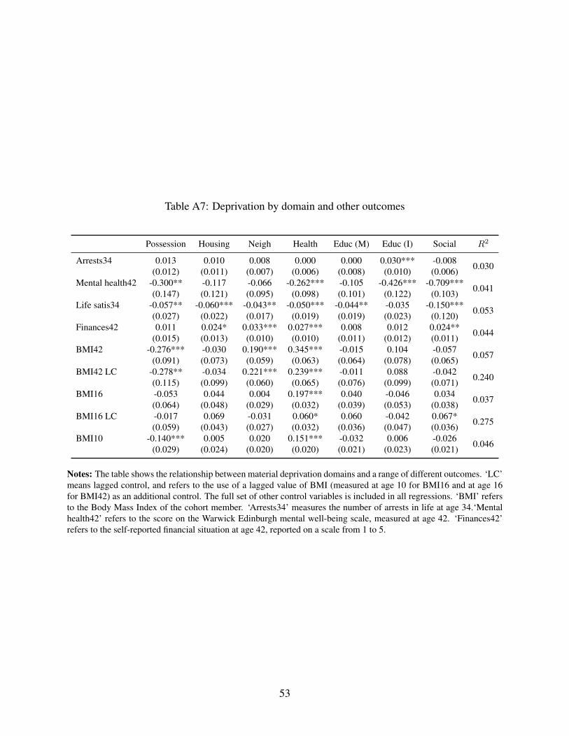
Table A7: Deprivation by domain and other outcomes

Possession Housing Neigh Health Educ (M) Educ (I) Social R2

Arrests34 0.013 0.010 0.008 0.000 0.000 0.030*** -0.008 0.030(0.012) (0.011) (0.007) (0.006) (0.008) (0.010) (0.006)Mental health42 -0.300** -0.117 -0.066 -0.262*** -0.105 -0.426*** -0.709*** 0.041(0.147) (0.121) (0.095) (0.098) (0.101) (0.122) (0.103)Life satis34 -0.057** -0.060*** -0.043** -0.050*** -0.044** -0.035 -0.150*** 0.053(0.027) (0.022) (0.017) (0.019) (0.019) (0.023) (0.120)Finances42 0.011 0.024* 0.033*** 0.027*** 0.008 0.012 0.024** 0.044(0.015) (0.013) (0.010) (0.010) (0.011) (0.012) (0.011)BMI42 -0.276*** -0.030 0.190*** 0.345*** -0.015 0.104 -0.057 0.057(0.091) (0.073) (0.059) (0.063) (0.064) (0.078) (0.065)BMI42 LC -0.278** -0.034 0.221*** 0.239*** -0.011 0.088 -0.042 0.240(0.115) (0.099) (0.060) (0.065) (0.076) (0.099) (0.071)BMI16 -0.053 0.044 0.004 0.197*** 0.040 -0.046 0.034 0.037(0.064) (0.048) (0.029) (0.032) (0.039) (0.053) (0.038)BMI16 LC -0.017 0.069 -0.031 0.060* 0.060 -0.042 0.067* 0.275(0.059) (0.043) (0.027) (0.032) (0.036) (0.047) (0.036)BMI10 -0.140*** 0.005 0.020 0.151*** -0.032 0.006 -0.026 0.046(0.029) (0.024) (0.020) (0.020) (0.021) (0.023) (0.021)

Notes: The table shows the relationship between material deprivation domains and a range of different outcomes. ‘LC’means lagged control, and refers to the use of a lagged value of BMI (measured at age 10 for BMI16 and at age 16for BMI42) as an additional control. The full set of other control variables is included in all regressions. ‘BMI’ refersto the Body Mass Index of the cohort member. ‘Arrests34’ measures the number of arrests in life at age 34.‘Mentalhealth42’ refers to the score on the Warwick Edinburgh mental well-being scale, measured at age 42. ‘Finances42’refers to the self-reported financial situation at age 42, reported on a scale from 1 to 5.

53

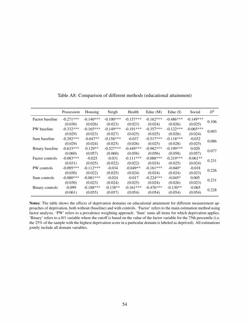
Table A8: Comparison of different methods (educational attainment)

Possession Housing Neigh Health Educ (M) Educ (I) Social R2

Factor baseline -0.271*** -0.140*** -0.100*** -0.157*** -0.162*** -0.486*** -0.149*** 0.106(0.030) (0.026) (0.023) (0.023) (0.024) (0.026) (0.025)PW baseline -0.332*** -0.165*** -0.149*** -0.191*** -0.357*** -0.122*** -0.065*** 0.093(0.029) (0.023) (0.027) (0.025) (0.025) (0.026) (0.024)Sum baseline -0.292*** -0.047** -0.158*** -0.037 -0.517*** -0.118*** -0.032 0.086(0.029) (0.024) (0.025) (0.026) (0.025) (0.028) (0.025)Binary baseline -0.633*** 0.129** -0.527*** -0.449*** -0.982*** -0.199*** 0.020 0.077(0.060) (0.057) (0.060) (0.056) (0.056) (0.058) (0.057)Factor controls -0.083*** -0.025 -0.031 -0.111*** -0.088*** -0.219*** -0.061** 0.231(0.031) (0.025) (0.022) (0.022) (0.024) (0.025) (0.024)PW controls -0.095*** -0.112*** -0.034 -0.049** -0.161*** -0.040* -0.018 0.226(0.030) (0.022) (0.025) (0.024) (0.024) (0.024) (0.023)Sum controls -0.080*** -0.081*** -0.024 -0.017 -0.224*** -0.045* 0.005 0.231(0.030) (0.023) (0.024) (0.025) (0.024) (0.026) (0.023)Binary controls -0.099 -0.188*** -0.138** -0.161*** -0.476*** -0.130** -0.065 0.228(0.061) (0.055) (0.057) (0.054) (0.054) (0.054) (0.054)

Notes: The table shows the effects of deprivation domains on educational attainment for different measurement ap-proaches of deprivation, both without (baseline) and with controls. ‘Factor’ refers to the main estimation method usingfactor analysis. ‘PW’ refers to a prevalence weighting approach. ‘Sum’ sums all items for which deprivation applies.‘Binary’ refers to a 0/1 variable where the cutoff is based on the value of the factor variable for the 75th percentile (i.e.the 25% of the sample with the highest deprivation score in a particular domain is labeled as deprived). All estimationsjointly include all domain variables.

54

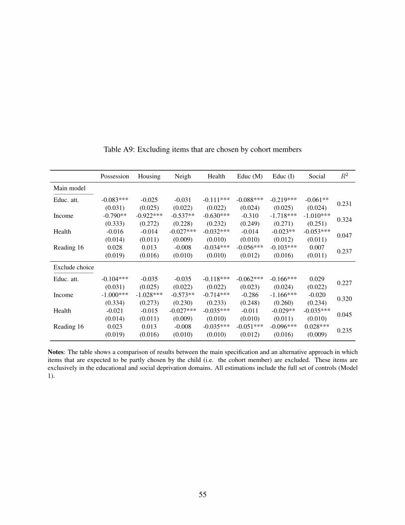
Table A9: Excluding items that are chosen by cohort members

Possession Housing Neigh Health Educ (M) Educ (I) Social R2

Main model

Educ. att. -0.083*** -0.025 -0.031 -0.111*** -0.088*** -0.219*** -0.061** 0.231(0.031) (0.025) (0.022) (0.022) (0.024) (0.025) (0.024)Income -0.790** -0.922*** -0.537** -0.630*** -0.310 -1.718*** -1.010*** 0.324(0.333) (0.272) (0.228) (0.232) (0.249) (0.271) (0.251)Health -0.016 -0.014 -0.027*** -0.032*** -0.014 -0.023** -0.053*** 0.047(0.014) (0.011) (0.009) (0.010) (0.010) (0.012) (0.011)Reading 16 0.028 0.013 -0.008 -0.034*** -0.056*** -0.103*** 0.007 0.237(0.019) (0.016) (0.010) (0.010) (0.012) (0.016) (0.011)

Exclude choice

Educ. att. -0.104*** -0.035 -0.035 -0.118*** -0.062*** -0.166*** 0.029 0.227(0.031) (0.025) (0.022) (0.022) (0.023) (0.024) (0.022)Income -1.000*** -1.028*** -0.573** -0.714*** -0.286 -1.166*** -0.020 0.320(0.334) (0.273) (0.230) (0.233) (0.248) (0.260) (0.234)Health -0.021 -0.015 -0.027*** -0.035*** -0.011 -0.029** -0.035*** 0.045(0.014) (0.011) (0.009) (0.010) (0.010) (0.011) (0.010)Reading 16 0.023 0.013 -0.008 -0.035*** -0.051*** -0.096*** 0.028*** 0.235(0.019) (0.016) (0.010) (0.010) (0.012) (0.016) (0.009)

Notes: The table shows a comparison of results between the main specification and an alternative approach in whichitems that are expected to be partly chosen by the child (i.e. the cohort member) are excluded. These items areexclusively in the educational and social deprivation domains. All estimations include the full set of controls (Model1).

55

Copyright © 2016 @ the author(s). Discussion papers are in draft form. This discussion paper is distributed for purposes of comment and discussion only. It may not be reproduced without permission of the copyright holder. Copies of working papers are available from the author.