DI

SC

US

SI

ON

P

AP

ER

S

ER

IE

S

Forschungsinstitut zur Zukunft der ArbeitInstitute for the Study of Labor

How Do Voters Respond to Information?Evidence from a Randomized Campaign

IZA DP No. 7340

April 2013

Chad KendallTommaso NanniciniFrancesco Trebbi

How Do Voters Respond to Information? Evidence from a Randomized Campaign

Chad Kendall University of British Columbia

Tommaso Nannicini

Bocconi University, IGIER and IZA

Francesco Trebbi

University of British Columbia, CIFAR and NBER

Discussion Paper No. 7340 April 2013

IZA

P.O. Box 7240 53072 Bonn

Germany

Phone: +49-228-3894-0 Fax: +49-228-3894-180

E-mail: iza@iza.org

Any opinions expressed here are those of the author(s) and not those of IZA. Research published in this series may include views on policy, but the institute itself takes no institutional policy positions. The IZA research network is committed to the IZA Guiding Principles of Research Integrity. The Institute for the Study of Labor (IZA) in Bonn is a local and virtual international research center and a place of communication between science, politics and business. IZA is an independent nonprofit organization supported by Deutsche Post Foundation. The center is associated with the University of Bonn and offers a stimulating research environment through its international network, workshops and conferences, data service, project support, research visits and doctoral program. IZA engages in (i) original and internationally competitive research in all fields of labor economics, (ii) development of policy concepts, and (iii) dissemination of research results and concepts to the interested public. IZA Discussion Papers often represent preliminary work and are circulated to encourage discussion. Citation of such a paper should account for its provisional character. A revised version may be available directly from the author.

IZA Discussion Paper No. 7340 April 2013

ABSTRACT

How Do Voters Respond to Information? Evidence from a Randomized Campaign*

Rational voters update their subjective beliefs about candidates’ attributes with the arrival of information, and subsequently base their votes on these beliefs. Information accrual is, however, endogenous to voters’ types and difficult to identify in observational studies. In a large scale randomized trial conducted during an actual mayoral campaign in Italy, we expose different areas of the polity to controlled informational treatments about the valence and ideology of the incumbent through verifiable informative messages sent by the incumbent reelection campaign. Our treatments affect both actual vote shares at the precinct level and vote declarations at the individual level. We explicitly investigate the process of belief updating by comparing the elicited priors and posteriors of voters, finding heterogeneous responses to information. Based on the elicited beliefs, we are able to structurally assess the relative weights voters place upon a candidate’s valence and ideology. We find that both valence and ideological messages affect the first and second moments of the belief distribution, but only campaigning on valence brings more votes to the incumbent. With respect to ideology, cross-learning occurs, as voters who receive information about the incumbent also update their beliefs about the opponent. Finally, we illustrate how to perform counterfactual campaigns based upon the structural model. JEL Classification: D72, D83 Keywords: voting, information, beliefs elicitation, randomized controlled trial Corresponding author: Tommaso Nannicini Department of Economics Bocconi University Via Roentgen 1 20136 Milan Italy E-mail: tommaso.nannicini@unibocconi.it

* We would like to thank Matilde Bombardini, David Green, Andrea Mattozzi, Jim Snyder, and seminar participants at Alicante, Bank of Italy, Bocconi, Carlo Alberto Turin, EIEF Rome, Harvard, LSE, MILLS workshop, MIT, Petralia workshop, Rotterdam, SciencesPo Paris, UBC, UK Leuven, and Warwick for useful comments. Federico Cilauro, Francesco Maria Esposito, Jonathan Graves, Nicola Pierri, and Teresa Talò provided outstanding research assistance. A large number of people were instrumental in implementing our experimental design: the mayor of Arezzo, Giuseppe Fanfani, and his 2011 reelection campaign, in particular Claudio Repek, were extremely cooperative throughout the entire process; Massimo Di Filippo, Fabrizio Monaci, and the team of “IPR Feedback” showed tremendous expertise in conducting the surveys. Nannicini acknowledges financial support from the European Research Council (under grant No. 230088). Remaining errors are ours and follow a random walk.

1 Introduction

We study the causal impact of campaign information on electoral outcomes and voters’ beliefs about

political candidates in the context of a large field experiment encompassing an entire electoral

campaign. In collaboration with the incumbent mayor of a medium-sized Italian city who was

running for reelection in 2011, eligible voters received hard and verifiable information, via mail

or phone, about the valence or the ideological stance of the incumbent. The city was randomly

divided into four areas, with the first receiving a campaign message about valence, the second

about ideology, the third about both valence and ideology, and the fourth receiving no message at

all. The informational treatments were administered by the incumbent as part of his campaign. Our

direct mailing covered the entire voting population and our phone bank covered about a quarter of

all households in the city. Moreover, voters received only our mailers from the incumbent campaign,

and only our phone calls from both the incumbent and the main challenger’s campaign.

Relative to the control group that received no campaign message, voters informed about the

valence of the incumbent—via both mail and phone—increased their support for the candidate by

4.1 percentage points as measured by precinct-level official vote shares, and by 9.5 percentage points

as measured by vote declarations in surveys. Much weaker effects on vote choices were detected

when information about the ideological stance of the incumbent was provided, or when campaigning

was done by mail only. To the best of our knowledge, this is the first time evidence from an entire

election has been used to answer the question of whether or not campaign information causally

influences actual electoral outcomes in a mature democracy.

This paper is not limited to the analysis of vote choices in the context of a randomized controlled

trial. Our goal is to show the extent of the response of individual agents to political messages and

to understand the degree of sophistication in their subjective updating. The empirical application

revolves around the assessment of the role of campaign ads in elections, but the point is more general

than political advertising. Our methodology can extend to other forms of direct communication

by politicians to voters, has implications beyond the political environment, and is of interest for

commercial advertising—or for any other type of informational treatment—as well.

Using a novel elicitation protocol, we collected information about the distributions of individual

voters’ (multivariate) beliefs about the valence and ideological stance of both the incumbent and

the main challenger through surveys both before and after the informational treatments were ad-

ministered. We show how, by imposing a limited amount of structure on electoral preferences and

belief distributions, prior and posterior beliefs of individual voters can be fully characterized. We

1

also show that, although only valence treatments were effective in changing votes, our informational

treatments along both the valence and ideological dimension had large effects on voters’ beliefs, mov-

ing both first and second moments of the belief distributions for the two main candidates. Indeed,

campaign information affected not only voters’ beliefs about the candidate originating the message,

but also their beliefs about the opponent. Intuitively, in Bayesian signaling games, receiving no

message is valuable information and our evidence on cross-learning appears fully consistent with

updating in the context of a Bayesian political signaling game.

The full characterization of the individual belief distributions we propose is the combination of a

careful design of our surveys and structural estimation of a random utility voting model. The latter

component of our methodology delivers precise estimates of utility weights in voters’ preferences

for a candidate’s valence and ideology. We report a utility weight on valence roughly equal to that

on ideological losses away from a voter’s bliss point. Interestingly, we also show that the preference

weights are heterogeneous in the population and depend on the political stance of the voter, with

voters on the right placing less emphasis on the valence dimension. Finally, we show that the

ideological loss function away from the voter’s bliss point is concave in distance, not convex (e.g.,

quadratic losses) as commonly assumed in the literature.

The random utility model we use follows the method outlined in the theoretical paper of Ramalho

and Smith (2012) to account for non-randomness in voters’ willingness to disclose their votes.

While non-response in survey data is often assumed to be random, we demonstrate the importance

of accounting for its endogeneity and suggest that this method should be more often utilized in

empirical studies in which survey responses are relied upon.

We conclude our analysis by simulating counterfactual electoral campaigns to assess the effects

of specific blanket or targeted electoral campaigns on vote outcomes. We find a blanket campaign

of valence messages to be the most valuable in persuading voters, which is consistent with voters

lacking prior information on the quality of candidates.

This paper is related to several strands of the literature. The effectiveness of electoral campaigns

in mature democracies is the subject of a large literature, including Ansolabehere et al. (1994),

Ansolabehere and Iyengar (1995), Gerber and Green (2000), Green and Gerber (2004), Gerber,

Green, and Shachar (2003), Nickerson (2008), and Dewan, Humphreys, and Rubenson (2010).

Typically the focus of these papers is either on self-declared outcomes for vote choices or on actual

outcomes for turnout. Methodologically, these papers rely on either small-scale experiments for

partisan ads or on randomized non-partisan campaigns for turnout. Our paper complements this

literature by focusing on actual electoral outcomes in a large scale field experiment. We must clarify

2

that our paper is not the first instance of a large scale randomized partisan campaign. Gerber et

al. (2011) look at randomization over intensity of TV ads (with no control over the message content)

on self-declared choices during the 2006 Republican primary for the Texas gubernatorial election.

They find large, but short-lived, effects of such TV ads, inconsistent with Bayesian updating. Unlike

their approach, we randomize the content of partisan ads and also evaluate their impact on actual

vote shares. Our paper also complements this literature from a methodological standpoint by

augmenting the reduced form approach with structural estimation.

Albeit in the context of less mature democracies, the literature in development economics has also

experimented with informational campaigning. Relevant contributions include Wantchekon (2003)

and Fujiwara and Wantchekon (2013), exploring political clientelism in Benin, Vicente (2013), and

Banerjee, Green, and Pande (2012). Banerjee et al. (2011) focus on non-partisan informational

campaigns in India and show that information about the qualifications of candidates matters for

turnout, vote shares, and the incidence of vote buying.

This paper is related to a vast literature on candidate’s valence, initiated by Stokes (1963) and

including Enelow and Hinich (1982), Ansolabehere and Snyder (2000), Groseclose (2001), Schofield

(2003), Aragones and Palfrey (2002) among others. More recently, Ashworth and Bueno de Mesquita

(2009), Kartik and McAfee (2007), and Bernhardt, Camara, and Squintani (2011) provide inter-

esting theoretical studies of strategic electoral competition with candidates differentiated along

both (ideological) policy platform and valence dimensions. Galasso and Nannicini (2011) study the

interplay between candidates’ valence and the contestability of electoral districts.

Finally, this paper contributes to the growing literature focused on the elicitation and quan-

tification of subjective beliefs. Elicitation of priors is the subject of Dominitz and Manski (1996),

Manski (2004), Blass, Lach, and Manski (2010), Gill and Walker (2005), and Duffy and Tavits

(2008) among others. To these contributions, which mostly focus on the elicitation of expectations

of economic outcomes, our work provides a useful addition in the context of the elicitation of mul-

tivariate beliefs. In particular, we show how to decouple information about marginal beliefs and

their dependence using a copula function approach. We believe this approach may be of use outside

the politico-economic application in our study.

The rest of the paper is organized as follows. Section 2 presents the empirical model. Section

3 describes the experimental setting. Section 4 discusses the reduced form results on vote choices.

Section 5 focuses on the structural estimates of the model and Section 6 on the experimental effects

on voters’ beliefs. Section 7 presents our counterfactuals and discusses the implications of the

heterogeneous response to information on the part of voters. Section 8 concludes.

3

2 Empirical Model

2.1 Voters and Candidates

Consider an electoral race between two candidates, A, the incumbent, and B, the challenger. Let

the set of voters be N , with |N | = N . A voter i is characterized by an ideal policy point distributed

over a finite and discrete policy space, Π, which is common across all voters, with policies P ∈ Π.

The discreteness assumption is meant to capture an empirical feature of the survey data employed

in the subsequent analysis. Voters are heterogeneous, with bliss points q ∈ Π, and receive disutility

from a policy choice away from their bliss point. They also receive utility from the level of valence

of the elected candidate V ∈ Λ, where the set Λ is finite and discrete. When policy p is implemented

by candidate j of valence v, the utility for voter i of type q is assumed to be:

U(v, p; q) = γv − u (q − p)− χu (q − p) v + εi,j

where the utility function includes a deterministic portion and a candidate-specific random utility

component εi,j , independent of V and P . The parameter γ indicates the relative preference weight

of valence versus the policy stance. We assume u (0) = 0, u′ (x) ≥ 0 for x > 0, and u′ (x) ≤ 0

for x < 0. For example, a quadratic loss away from voter i’s bliss point, (qi − p)2, fits this set

of assumptions.1 However, we assume the more general form u (x) = |x|ζ with ζ ≥ 0. The policy

stance of the politician, p, affects voters heterogeneously depending upon their own ideal position, q,

but candidates of higher quality v are favored by all voters. We also allow for interactions between

valence and policy positions that are governed by χ. The random utility component εi,j of voter i’s

preferences for candidate j captures the personal appeal of j to i.

It is not important for our purposes to specify whether the two candidates A and B implement

their respective ideal policy position P once in office (see Ansolabehere, Snyder, and Stewart, 2001;

Lee, Moretti, and Butler, 2004) or strategically cater their policy to voters (e.g., as in a standard

Downsian setting). We are interested in the voters’ utilities at the time they place their vote, which

only depend upon their beliefs about each candidate’s position, and not on how the policy position

came about or whether or not it is actually implemented. In general, our approach is robust to the

details of the electoral competition structure.

All voters participate in the election (voting is compulsory in our empirical setting). Voter i is

assumed to have a joint prior distribution function over V and P , f i,jV,P (v, p), for j = A,B, evaluated

at point (v, p) and defined over the support Λ × Π. We do not preclude V from being potentially

correlated with P and we allow priors to differ based upon i’s characteristics or ideal point q.1Quadratic loss functions are standard in the literature (e.g., see Ansolabehere and Snyder, 2000).

4

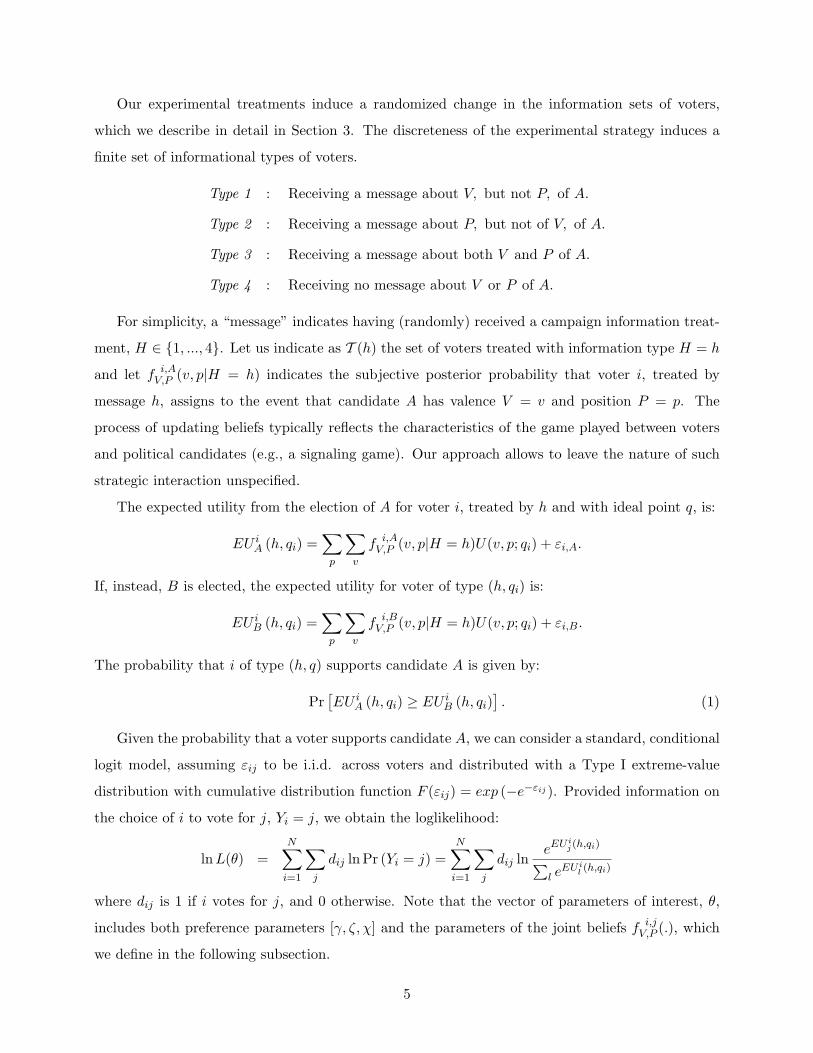
Our experimental treatments induce a randomized change in the information sets of voters,

which we describe in detail in Section 3. The discreteness of the experimental strategy induces a

finite set of informational types of voters.

Type 1 : Receiving a message about V, but not P, of A.

Type 2 : Receiving a message about P, but not of V, of A.

Type 3 : Receiving a message about both V and P of A.

Type 4 : Receiving no message about V or P of A.

For simplicity, a “message” indicates having (randomly) received a campaign information treat-

ment, H ∈ {1, ..., 4}. Let us indicate as T (h) the set of voters treated with information type H = h

and let f i,AV,P (v, p|H = h) indicates the subjective posterior probability that voter i, treated by

message h, assigns to the event that candidate A has valence V = v and position P = p. The

process of updating beliefs typically reflects the characteristics of the game played between voters

and political candidates (e.g., a signaling game). Our approach allows to leave the nature of such

strategic interaction unspecified.

The expected utility from the election of A for voter i, treated by h and with ideal point q, is:

EU iA (h, qi) =

∑p

∑v

f i,AV,P (v, p|H = h)U(v, p; qi) + εi,A.

If, instead, B is elected, the expected utility for voter of type (h, qi) is:

EU iB (h, qi) =

∑p

∑v

f i,BV,P (v, p|H = h)U(v, p; qi) + εi,B.

The probability that i of type (h, q) supports candidate A is given by:

Pr[EU i

A (h, qi) ≥ EU iB (h, qi)

]. (1)

Given the probability that a voter supports candidate A, we can consider a standard, conditional

logit model, assuming εij to be i.i.d. across voters and distributed with a Type I extreme-value

distribution with cumulative distribution function F (εij) = exp (−e−εij ). Provided information on

the choice of i to vote for j, Yi = j, we obtain the loglikelihood:

lnL(θ) =N∑

i=1

∑j

dij ln Pr (Yi = j) =N∑

i=1

∑j

dij lneEU i

j(h,qi)∑l e

EU il (h,qi)

where dij is 1 if i votes for j, and 0 otherwise. Note that the vector of parameters of interest, θ,

includes both preference parameters [γ, ζ, χ] and the parameters of the joint beliefs f i,jV,P (.), which

we define in the following subsection.

5

One potential problem with the standard logit model in a setting employing vote declarations as

opposed to actual votes is that voters, when surveyed, may prefer not to disclose their vote. If the

sample of voters who do not disclose their vote is completely random, one can apply the logit model

to the subsample of responders. This is the approach typically followed in the literature, often

without diagnostics in support of the crucial “missing completely at random” assumption, required

for an unbiased estimate. We provide evidence in Section 5 that indicates that the subsample of

voters that choose not to disclose their votes is predictable, so estimation of the standard logit model

would lead to biased estimates in our setting. We therefore apply a novel choice-based approach

suggested by Ramalho and Smith (2012) that allows for non-random non-response under weak

assumptions. The model assumes that, conditional on the voter’s actual vote, the probability with

which a voter chooses to respond to the survey is constant, but that this probability can depend on

their vote. Under this assumption, we can define the loglikelihood as:

lnL(θ) =N∑

i=1

oi

∑j

dij lnβjeEU i

j(h,qi)∑l e

EU il (h,qi)

+ (1− oi) ln

1−∑

j

βjeEU i

j(h,qi)∑l e

EU il (h,qi)

where oi is 1 if i discloses the vote, and 0 otherwise. The additional βj parameters are the probabil-

ities with which a voter discloses the vote for j. The first term of the loglikelihood is the probability

that a voter votes for j and discloses the vote. The second term reflects the probability that the

voter votes for one of the candidates, but chooses not to disclose the vote. Note that when βj = 1

for all j, such that the vote is always observed, we obtain the standard logit model as a special case.

Our results in Section 5 reject βj = 1 for all j, meaning that we are justified in accounting for the

possibility of non-random non-response.

2.2 Voters’ Subjective Updating

Here, we specify the process by which voters’ subjective beliefs are updated in the presence of

campaign advertising. For illustrative purposes, consider the following time line.

6

Our first assumption is that voters consider the campaign information to be truthful. Sufficient

freedom of the press in the Italian electoral context guarantees that such an assumption may be

valid in the case of factual advertising, as we employ in our experimental setup. All messages are

factual and can be independently validated.

Secondly, we assume rational Bayesian voters.2 We refrain from imposing distributional as-

sumptions on priors, posteriors, and on the distribution of signals. Instead, we adopt the option of

eliciting subjective priors and posteriors from specifically designed surveys. This is an important

step for two main reasons. First, elicitation allows us to assess quantitatively how the messaging

strategy we employed experimentally operates in the field. Indeed, voters are not aware of the ran-

domization process and update their beliefs “as if” the messages were directly sent by the candidate.

This is not an assumption, but part of the experimental design. Under the assumption of Bayesian

voters, belief updating about candidate A implies:

f i,AV,P (v, p|H = h) =

Pri,A (H = h|V = v, P = p)Pri,A (H = h)

× f i,AV,P (v, p) for h = 1, 2, 3,

where the subjective updating term Pri,A(H=h|V =v,P=p)

Pri,A(H=h)can be recovered directly from the data after

elicitation of f i,AV,P (v, p|H = h) and f i,A

V,P (v, p). Second, our approach allows for general strategic

electoral communication between candidates and voters in the background. We are not required to

model or restrict the voting game played among N , A, and B. Any strategic signaling is captured

by the updating term Pri,A(H=h|V =v,P=p)

Pri,A(H=h), which we estimate, not model.3

Bayesian updating in case the voter receives no message from the candidate requires further

discussion. Consider the case of a fully rational Bayesian voter that receives no campaign advertising

from a candidate, but knows that such action was available. In such a case, as Chappell (1994)

states, “absence of a message provides information which should be used in Bayesian updating”

with the result that subjective posteriors probabilities are different from priors even absent any

message having reached the voter. In the case of posteriors about candidate B, for instance, this

requires that voter i updates priors based on absence of an H message from B. Formally:

f i,BV,P (v, p|H = h) 6= f i,B

V,P (v, p) for h = 1, 2, 3, (2)

which is justified from voter i having observed at least one extra campaign message from A without

any corresponding counter-message from B.2Note that, while we need voters to be rational and vote sincerely, the assumption of Bayesian updating is simply

convenient for the exposition, as our empirical framework allows us to identify belief updating in more general terms.3A dynamic repeated election model with both ideological and valence considerations that would fit our problem

is, for instance, proposed in Bernhardt, Camara, and Squintani (2011).

7

The degree of rationality embedded in condition (2) cannot be extended, however, to the exper-

imental control group H = 4, which does not receive any type of informational treatment by either

A or B and hence has no possibility of knowing that such specific messages would be available but

were not employed. The fundamental assumption of our experimental design mirrors a Stable Unit

Treatment Value Assumption (SUTVA, see Cox, 1958; Rubin, 1978), as it requires the potential

outcome of a control unit to be unaffected by the treatment assignment of the other units. Absent

common shocks, we should assume for H = 4 that the posterior distribution is identical to the prior

distribution, that is, for every i ∈ T (4), f i,jV,P (v, p|H = 4) = f i,j

V,P (v, p) for j = A,B.

More generally, we consider a process of Bayesian updating which accommodates common shocks

across voters, under the (testable) assumption that the subjective probabilities on such shocks are

identical across all i ∈ N and independent of H. Consider, for instance, the case of posteriors

elicited after a common informational shock, W , which can be thought of as the general campaign

carried out by the candidates besides the informational messages from A that we randomize at the

margin. With respect to candidate j, voter i will be characterized by the following posteriors.

Assumption 1 (SUTVA): f i,jV,P (v, p|H = h, W ) =

Pri,j (H = h|V = v, P = p)Pri,j (H = h)

×Prj (W |V = v, P = p)Prj (W )

× f i,jV,P (v, p) for h = 1, 2, 3; j = A,B

and

f i,jV,P (v, p|H = 4,W ) =

Prj (W |V = v, P = p)Prj (W )

× f i,jV,P (v, p) for j = A,B.

The credibility of Assumption 1 crucially rests on the experimental design described in Section 3

and is empirically validated in Section 4.

Finally, the elicitation of multivariate beliefs, even on expert subjects, is not an obvious exercise

(Kadane and Wolfson, 1998; Garthwaite et al., 2005) and is the object of a vast literature bordering

statistics and psychology (dating at least as back as Savage, 1971). We outline our approach next.

2.3 Elicitation of Multivariate Beliefs

Elicitation of beliefs and priors is increasingly common in economics and political science, and is

standard in psychology and statistics.4 We describe a transparent protocol of elicitation we designed

to be robust to the behavioral and technological constraints we face. Specifically, we sampled a large

number of voters and need to elicit multivariate beliefs from each.4For recent examples in economics, see Dominitz and Manski (1996); Manski (2004); Blass et al. (2010); and Zafar

(2009). See Gill and Walker (2005) and Duffy and Tavits (2008) for applications in political science.

8

For each main candidate j = A,B and each voter i, joint valence and ideology subjective

priors f i,jV,P (v, p) and posteriors f i,j

V,P (v, p|H = h) are defined over Λ × Π. In the remainder of this

subsection, let us focus for brevity on the elicitation of subjective priors, with the understanding

that the same process applies to posteriors. In the empirical analysis we will fix the cardinality

of both Λ and Π to small integer figures, based on Miller (1956), and a large body of cognitive

psychology suggesting that individuals can be quite precise in evaluating choices on relatively coarse

unidimensional supports, but display hardly any precision on finer supports. Specifically, for reasons

explained below, we assume the cardinality of Π to be equal to 5 and the cardinality of Λ to be

equal to 10.

It is evident, however, that even for |Π| = 5 and |Λ| = 10, “brute force” elicitation for both

candidates would require each responder to answer 5 × 10 × 2 = 100 different questions on the

subjective likelihood of each specific (v, p) realization, an effort which would likely frustrate political

experts, let alone regular voters. Garthwaite, Kadane, and O’Hagan (2005) present an insightful

discussion on the difficulty of elicitation for multivariate priors. To this issue, the reader versed

in elicitation may add the problem of effectively training telephone interviewers in the consistent

elicitation of joint probabilities.5 Therefore, we follow an alternative route.

2.3.1 Marginal Belief Distributions

We first focus on information more easily elicitable from voters: the univariate marginals f i,jV (v) and

f i,jP (p). Even in this case, full elicitation of marginals would require a large set of (|Π|+ |Λ|)×2 = 30

questions. We streamline the process in order to maintain feasibility without excessive sacrifice of

accuracy. We start by imposing a simple regularity assumption on the distribution of beliefs.

Assumption 2 : Subjective belief distributions are unimodal.

Although restrictive, this assumption makes the interpretation of the elicited probabilities more

direct. All of our remaining distributional assumptions can be illustrated using the questions in

our surveys by way of example. We focus only on A for brevity and consider first his ideological

position P . We enquire about the central tendency of the marginal prior on ideology as follows.

Q1 : How would you most likely define candidate A’s political position?

Left (1); Center-Left (2); Center (3); Center-Right (4); Right (5); Don’t Know (− 999).

5While the use of telephone interviews is not generally necessary, in our context it is was required to ensure timelyelicitation of a large sample of the voting population as close as possible to election day.

9

A reasonable interpretation of the answer, with minimal confusion for the respondent, is that the

mode is elicited. In particular, we allow the mode, p, to be only one of these five categories.

Assumption 3 : Π = {1, ..., 5} .

An answer of “Don’t Know/Don’t Know A” implies flat priors, or f i,AP (p) = 1/ |Π| = 0.2 for every

p. Our choice of the set Π follows the established result in cognitive psychology that individuals are

well versed in choices over discrete sets of limited dimensionality (|Π| ≤ 10), but that this capacity

deteriorates sharply when the number of options rises above small integers (Miller, 1956). Such an

assumption, however, has costs, as emphasized in Manski and Molinari (2010).

Conditional on non-flat priors, we further enquire about the dispersion around the mode.6

Q2 : How large is your margin of uncertainty around candidate A’s political position?

Certain (1); Rather uncertain, leaning left (2); Very uncertain, leaning left (3);

Rather uncertain, leaning right (4); Very uncertain, leaning right (5).

We indicate the level of increasing tightness of the priors with s ∈ Σ = {1, ..., 4}, where s = 1 is

maximal dispersion, i.e., the case of flat priors; s = 2 indicates substantial uncertainty (answers

3 or 5 to Q2); s = 3 indicates intermediate uncertainty (answers 2 or 4 to Q2); and s = 4 is

maximal tightness, which coincides with a degenerate prior spiking at p (answer 1 to Q2). Q2 also

elicits information about the skew of the beliefs. While we do not allow explicitly for an answer of

symmetric dispersion for s = 2, 3, not to overload the responder, the estimation below allows for

symmetric belief distributions.7 Let us indicate with z ∈ {−1; 1} a negative (i.e., to the left/lower

values) or positive (i.e., to the right/higher values) asymmetry in Q2.

Let us define the modal probability mass with φP = f i,AP (p = p). Intuitively, we assume the

probability mass at the mode f i,AP (p = p) is lower the higher the level of uncertainty. We allow φP

to vary with s and estimate φP,s, from the data for s = 2, 3, imposing the bounds:

Assumption 4 : 1/ |Π| ≤ φP,2 ≤ φP,3 ≤ 1.

We further assume the off-mode mass, 1 − φP,s, to be allocated asymmetrically around the mode

depending on the indicated asymmetry, z. We assume the off-mode mass decays proportionally6Interviewers were trained during pilot interviews to explain to voters that this question entailed uncertainty about

subjective evaluations on the candidates, and should not be interpreted as a right-or-wrong question.7In our surveys, we actually included a possible answer “uncertain” to assess the share of respondents indicating

symmetric dispersion around the mode. The share of respondents in that category was so low for ideology (andactually none for valence) that we omit it from exposition.

10

to the distance |p− p| from the mode at a constant rate, as dictated by a function g(x1, x2):

{1, ..., |Π| − 1} × [0, 1] → [0, 1] with gx1(x1, x2) ≥ 0 and gx2(x1, x2) ≤ 0. In synthesis, we impose:

Assumption 4’ : f i,AP (p 6= p) =

1/ |Π|

g (φP,s, z ∗ (p− p))0

for s = 1for s = 2, 3for s = 4.

Concerning g(.), we allocate αP (1− φP,s) mass in the direction of the asymmetry imposing that

αP ∈ [1/2, 1], and allocate (1− αP ) (1− φP,s) in the opposite direction, assuming a linear decay

of the off-mode mass in both directions. This specification of g allows for a very flexible, but

parametrically parsimonious marginal distribution.

Concerning the valence dimension V , we again enquire about the modal belief.

Q3 : Setting aside his/her political position, how would you most likely grade candidate A?

From 1 (minimum competence) to 10 (maximum competence) or Don’t Know (− 999).

The set Λ is then assumed to be as follows:

Assumption 5 : Λ = {1, ..., 10} .

This particular format of Q3 was driven by the familiarity of Italian voters with primary and

secondary education grade scoring rules, with 10 indicating the best possible mark in a school

assignment and failing grades being below 6. The dispersion around the valence mode and the

skewness of valence beliefs are modeled similarly to Assumptions 4 and 4’ with Λ replacing Π in

the construction of f i,AV (v). We omit their description for brevity. For illustrative purposes, Figure

1 provides an example of the modeled prior beliefs about the valence of A for one particular voter.

The distribution in the figure is based upon the voter’s reported mode (p = 7) and uncertainty

(s = 2) and the estimates we obtain for the parameters governing the distribution.

Finally, we must emphasize that we only elicit the beliefs about valence and ideology for the

incumbent candidate, A, and his main challenger, B, due to the infeasibility of eliciting beliefs

about all minor, third-party candidates participating in the election. In our estimation in Section

5, we assume that the beliefs of all non-incumbent candidates are the same as those elicited for

the main challenger, B. While this is a stark assumption, we justify it by the fact that the main

non-incumbent candidates were ideologically similar and their qualities were relatively unknown

(flat beliefs along the valence dimension are quite common for non-incumbent candidates).8

8The main third-party challenger was also a right-wing candidate, like B, but was sidelined by their party due topending legal litigation related to his previous stint in office. See Section 3 for more institutional details.

11

2.3.2 Joint Belief Distributions: A Copula-Based Approach

Having derived the univariate marginals, we now derive the joint distributions for all voters. Given

any two (univariate) marginals, it is possible to construct a joint (bivariate) distribution in infinite

ways. Copulas, introduced by Sklar (1959), are useful devices for providing a representation of a

multivariate distribution function in terms of its univariate marginal distributions.

Dropping the superscripts, given cumulative marginals, FV (v) = Pr(V ≤ v) and FP (p) =

Pr(P ≤ p), a copula function C satisfies FV,P (v, p) = C(FV (v), FP (p)) where FV,P (v, p) = Pr(V ≤

v, P ≤ p) is the joint cumulative distribution function. C is unique for continuous densities. For dis-

crete densities, as in our setting, typically the same joint distribution can be represented by different

copulas, but a specific copula uniquely identifies a joint distribution. The marginal distributions

carry all of the information related to the scaling and shape of the joint distribution function, while

the copula function incorporates the information concerning the dependence relationship among

the random variables. For parsimony, we will focus on copula families characterized by one depen-

dence parameter. Notice, however, that the dependence parameter does not coincide with a linear

correlation parameter; nonlinear dependence is accommodated as well.

We investigate three popular types of copulas, allowing for different degrees of association ρ

between V and P . First, independence between V and P produces the intuitive copula FV,P (v, p) =

FV (v)∗FP (p). Second, we allow for common dependence across surveyed voters, given by association

parameter −1 ≤ ρ ≤ 1, employing the Farlie-Gumbel-Morgensen (1960) family copula, FV,P (v, p) =

FP (p) ∗ FV (v) ∗ (1 + ρ(1 − FP (p)) ∗ (1 − FV (v))), where ρ > 0 implies positive dependence and

ρ < 0 negative dependence. Potentially, ρ could be made voter-type dependent (e.g., allowing for a

different ρ for left and right-wing voters), but not voter-specific. The FGM family is flexible, but

allows only small departures from independence. The third type of copula family we consider is the

Frank family, FV,P (v, p) = 1/ξ ∗ log(1 + D(ξ)), with D(ξ) = (eξFP (p) − 1)(eξFV (v) − 1)/(eξ − 1) and

ρ = −ξ. The Frank family allows larger departures from independence and requires ρ 6= 0. Indeed,

the Frank copula is well suited to model outcomes with strong positive or negative dependence.

The dependence parameter ρ is not elicited from the survey, but can be estimated from the data.

Recall that we observe vote decisions and such decisions are function of the voters’ posteriors. Given

a copula family, we can estimate a dependence parameter ρ as part of the vector of parameters, θ,

by maximizing the likelihood of observing those votes as in equation (1). One can further employ

standard generalized likelihood ratio tests to assess the relative quality of the assumptions on the

copula family and select the preferred family. We follow this approach.

12

To summarize, our set of parameters of interest is θ = [βA, βB, γ, ζ, χ, θ′] with belief parameters

θ′= [φP,2, φV,2, φP,3, φV,3, αP , αV , ρA, ρB], where we allow the association parameter to be different

for A and B. Estimating θ′ from vote decisions is only feasible for the posterior joint distribution.

The prior joint distribution can be fully characterized under an additional assumption.

Assumption 6 : Subjective belief distributions have constant θ′.

In particular, while we allow marginals to be affected by our informational treatment, we assume that

the dependence between ideology and valence of the candidate is constant. For example, assuming

that a moderate policy stance is positively correlated with smarter candidates, information that

moves subjective priors toward higher levels of valence V is allowed to have an impact on the policy

stance P , pushing it toward a more moderate stance, but it is not allowed to change the association

between P and V .9

Figure 2 and Figure 3 provide an example of the joint distributions for a particular voter’s

beliefs about candidate A prior to the election campaign and after receiving the valence message

treatment. Each joint distribution is determined assuming independence of the marginals and

based on the estimates of the parameters governing the marginal distributions. For this particular

voter, receiving the valence message increased his belief about the valence of A and also reduced

the uncertainty along both dimensions. In Section 6, we will see that such changes in beliefs are

representative of voters receiving the valence message treatment.

3 Experimental Design

In May 2011, in collaboration with the reelection campaign of the incumbent mayor in the Italian

city of Arezzo, we implemented the experimental strategy embedded in the above empirical model

during the mayor’s actual electoral campaign. Specifically, we divided the city into four areas,

randomizing at the precinct level, and the incumbent sent different campaign messages both by

mail and by phone call to voters in these areas. In this section, we describe the institutional setting,

as well as the nature of the (randomized) campaign messages and tools.

3.1 Institutional Setting

In Italy, mayors of cities with more than 15,000 inhabitants are directly elected under a plurality

system with runoff, that is, in the first round the candidate who obtains more than 50 percent of the9As an alternative to Assumption 6, one could calibrate ρj for the prior distribution at specific values and observe

the sensitivity of the results. A natural range of values could be the confidence interval of the dependence parameterfor the posteriors. We do not pursue this avenue here.

13

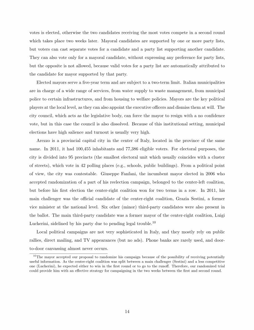
votes is elected, otherwise the two candidates receiving the most votes compete in a second round

which takes place two weeks later. Mayoral candidates are supported by one or more party lists,

but voters can cast separate votes for a candidate and a party list supporting another candidate.

They can also vote only for a mayoral candidate, without expressing any preference for party lists,

but the opposite is not allowed, because valid votes for a party list are automatically attributed to

the candidate for mayor supported by that party.

Elected mayors serve a five-year term and are subject to a two-term limit. Italian municipalities

are in charge of a wide range of services, from water supply to waste management, from municipal

police to certain infrastructures, and from housing to welfare policies. Mayors are the key political

players at the local level, as they can also appoint the executive officers and dismiss them at will. The

city council, which acts as the legislative body, can force the mayor to resign with a no confidence

vote, but in this case the council is also dissolved. Because of this institutional setting, municipal

elections have high salience and turnout is usually very high.

Arezzo is a provincial capital city in the center of Italy, located in the province of the same

name. In 2011, it had 100,455 inhabitants and 77,386 eligible voters. For electoral purposes, the

city is divided into 95 precincts (the smallest electoral unit which usually coincides with a cluster

of streets), which vote in 42 polling places (e.g., schools, public buildings). From a political point

of view, the city was contestable. Giuseppe Fanfani, the incumbent mayor elected in 2006 who

accepted randomization of a part of his reelection campaign, belonged to the center-left coalition,

but before his first election the center-right coalition won for two terms in a row. In 2011, his

main challenger was the official candidate of the center-right coalition, Grazia Sestini, a former

vice minister at the national level. Six other (minor) third-party candidates were also present in

the ballot. The main third-party candidate was a former mayor of the center-right coalition, Luigi

Lucherini, sidelined by his party due to pending legal trouble.10

Local political campaigns are not very sophisticated in Italy, and they mostly rely on public

rallies, direct mailing, and TV appearances (but no ads). Phone banks are rarely used, and door-

to-door canvassing almost never occurs.10The mayor accepted our proposal to randomize his campaign because of the possibility of receiving potentially

useful information. As the center-right coalition was split between a main challenger (Sestini) and a less competitiveone (Lucherini), he expected either to win in the first round or to go to the runoff. Therefore, our randomized trialcould provide him with an effective strategy for campaigning in the two weeks between the first and second round.

14

3.2 Randomized Campaign

To operationalize our informational treatments, we studied the campaign materials of the incumbent

and assembled relevant information so as to isolate slogans based on either his competence as city

manager (valence message) or his political stance (ideology message). Because we wanted to stay

away from the strategic game between him, the other candidates, and the voters (that is, we

wanted to randomize his actual campaign), we actually devised two different ideological messages:

one leaning toward the left and one leaning toward the center of the political spectrum. We then

allowed him to choose between the two and he selected the leftist message.

Furthermore, although our treatment of interest coincides with partisan campaign messages

delivered by one of the candidates, as opposed to non-partisan information, we wanted our informa-

tional treatments to be factual and non-emotional, as typical for cheap or costly signaling games.11

For this reason, we matched the main slogans with bullet points based on verifiable information

about the incumbent’s performance and policy choices during his first term in office. Future research

should extend to emotional messages as well, but we did not explore this avenue here.

Appendix Figures A1 and A2 show the mail flyers containing the two messages.12 The valence

flyer is built around two keywords: competence and effort. The implicit message is that voters

should reelect the incumbent because he was competent and effective as city manager. The factual

information provided refers to the fact that Arezzo developed an urban development plan that was

ranked first by the regional government and received extra funding because of its quality. The extra

funding was used to rebuild monuments, roads, and parking slots in the city center. The ideology

flyer is built around two keywords: awareness and solidarity. The implicit message is that voters

should reelect the incumbent because he shares values that are commonly associated with the Italian

left. The bullet points further reinforce the leftist tone as they point to “public” services, such as

childcare and food facilities for the poor, that were expanded during his first term in office.13 Notice

that the two mail flyers are identical in size, layout, colors, fonts, number of words, and photo of

the candidate; only the content of the campaign message differs.11The marketing and advertising literature (see Liu and Stout, 1987) has explored subjective responses to factual

versus emotional or nonfactual messages, indicating systematic differences. As an interesting counter, Gerber etal. (2011) present a randomized trial involving nonfactual campaign messages.

12In the Appendix, we also report the English translation of the text of the two flyers. Additional materials relatedto our randomized campaign can be found on the website: www.igier.unibocconi.it/randomized-campaign.

13To validate our operationalization of the two informational treatments ex ante, we randomly assigned the twoflyers to 50 university students at Bocconi University (in Milan) who did not know the mayor of Arezzo. We then askedthem to give their subjective assessment of the politician’s valence and ideology using the same questions describedin Section 2. For the 25 students who received the first message, the average valence evaluation was 6.650 (s.d. 0.963)and the average ideology evaluation was 3.100 (s.d. 0.700). For the 25 students who received the second message,these values were 5.450 (s.d. 0.973) and 2.050 (s.d. 0.669), respectively.

15

The two campaign messages—valence and ideology—were supplied to voters in two ways, through

direct mailing and phone calls. The randomization design was implemented as follows. We ran-

domly divided the 95 precincts into four groups: (i) 24 precincts received the valence message; (ii) 24

precincts received the ideology message; (iii) 24 precincts received both messages; (iv) 23 precincts

received no message (control group). Furthermore, we randomly split the first three groups into

two subgroups: in the first, the treatment was administered by both direct mail and phone calls

(12 precincts); in the second, by direct mail only (12 precincts).14

Appendix Table A1 reports the ex-ante balance tests of predetermined variables at the precinct

level. The available variables include the number of eligible voters enlisted in each precinct, the

city-wide neighborhood each precinct belongs to, and past electoral outcomes of national, regional,

European, and municipal elections. As precincts were reshuffled in the last decade, some outcomes

are not available for all 95 precincts. All of the predetermined variables are balanced across treat-

ment groups. Only the number of eligible voters displays a coefficient significant at the 10 percent

level, because of the presence of a few small precincts in the countryside that could not be spread

across all groups. Removing these precincts from the analysis, however, does not alter the results.

In order to increase the effectiveness of the campaign messages, we drew useful insights from the

U.S. experimental evidence summarized by Green and Gerber (2004). First, we acted in the week

before election day, so as to ensure the message sticks in voters’ minds. Second, we had our mail

flyers designed by professionals and directly sent to individuals with their name and address on the

envelope.15 Third, we did not use automated robo calls. We instead trained volunteers to make the

campaign phone calls. Specifically, from the candidate’s headquarters, volunteers called all selected

households with the following protocol: first, they were instructed to talk with the voters and ask

for their opinion for about two minutes. Then, they would ask the voter to listen to a recorded

message from the candidate. At the end of the call, the recorded voice of the candidate read a

30-second script with the above valence and ideology messages (or a combination of the two).16

Our randomized campaign used the above tools—mailers and phone calls—on a large scale. All

households in the city received an envelope from the incumbent campaign. The envelope contained

the official platform of the political parties supporting the candidate plus one of our flyers (or both

of them) according to the assigned treatment group. Voters in the control group received just the14As we were already pushing the boundaries in terms of sample size, we decided that the accuracy loss could not

justify an additional subgroup treated by phone calls only.15To avoid sending multiple envelopes to the same household, we randomized the name of the receiver within each

household, because we did not want to target only household heads.16In the Appendix, we report the English translation of the text of the three recorded messages. Original audio

files are available on the website: www.igier.unibocconi.it/randomized-campaign.

16

platform, but not the flyer with our informational treatment. This procedure allowed us to keep the

candidate unaware of the randomization outcome. Of course, the candidate approved all messages

and paid for the costs of the campaign, but we gave him closed envelopes so that he could not infer

which precincts were receiving one flyer as opposed to the other. In summary, all households with

at least one member enlisted as an eligible voter received our mailers. On top of this, about 25

percent of the households in the treatment groups also received a campaign phone call.17

3.3 Data

To elicit beliefs about the valence and ideology of the two main candidates along the lines described

in Section 2, we ran two surveys of 2,042 eligible voters distributed across all treatment groups.

We ran the first survey ten days before the election and, most importantly, before voters received

the informational treatments, so as to measure priors and demographic characteristics. The second

survey was conducted the day after the election and was meant to measure posteriors and (self-

declared) vote choices. To implement our surveys, we contracted a company from another Italian

region, so as to have interviewers with different accents from the campaign volunteers and to remove

any link between the campaign and the survey phone calls. About 71 percent of the respondents in

the first survey also replied to the question about whether they voted or not in the second survey.

Therefore, our sample is made up of 1,455 voters, 1,306 of whom actually voted for one of the

candidates. However, 231 of the 1,306 voters did not specify for which candidate they voted and for

this reason we accommodate for potentially non-random non-responses in the model estimation.

To further validate our randomization design ex post, we checked for balancing of the charac-

teristics of voters across treatment groups. Survey variables include demographic characteristics,

educational attainment, political orientation, home ownership, and how often voters read newspa-

pers or watch TV. The results are reported in Appendix Table A2. None of these (self-declared)

individual characteristics is statistically different across treatment groups.18

Table 1 summarizes election results at the precinct level. The incumbent mayor won his bid

for reelection with a vote share 51.3 percent, enough to avoid a run off. Table 2 shows the (self-17Because of budget and time constraints, we could not reach all households by phone.18As an additional ex-post validation of the randomization design, we built proxies of Census characteristics at the

precinct level. This exercise has two limitations, however. First, data from the last available Census refer to 2001.Second, precincts are not easily matchable with Census cells. To overcome the second limitation, we implementedthe following geocoding procedure: 1) for each street (i.e., line) belonging to a precinct we calculated the weightedaverage of the characteristics of the Census cells (i.e., polygons) overlapping with that street (with weights equal to theoverlapping segments); 2) for each precinct, we calculated the weighted average of the characteristics of the associatedstreets (with weights equal to the population living in each street). Appendix Table A3 reports the balancing testsof these Census characteristics across treatment groups. Although the estimates are likely to suffer from attenuationbias due to measurement error, none of them is statistically different from zero.

17

declared) vote choices of surveyed individuals. As often happens in post-electoral polls, there is a

slight bandwagon effect in vote declarations favoring the winning candidate (57.1 percent). The

bandwagon is not a concern for estimation under the (plausible) assumption that this effect is

orthogonal to our treatment groups. In any case, recall that a strength of our approach is that we

can cross-validate the consistency of treatment effects in the survey data (at the individual level)

with those in the aggregate actual voting data (at the precinct level).

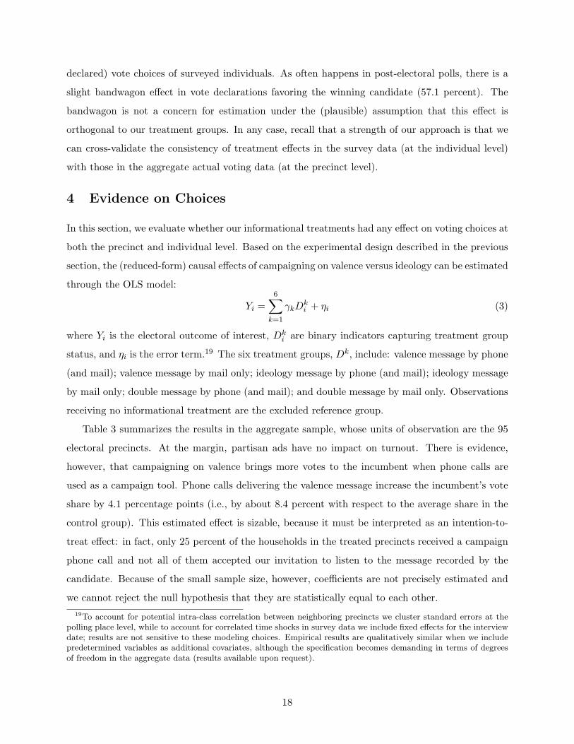
4 Evidence on Choices

In this section, we evaluate whether our informational treatments had any effect on voting choices at

both the precinct and individual level. Based on the experimental design described in the previous

section, the (reduced-form) causal effects of campaigning on valence versus ideology can be estimated

through the OLS model:

Yi =6∑

k=1

γkDki + ηi (3)

where Yi is the electoral outcome of interest, Dki are binary indicators capturing treatment group

status, and ηi is the error term.19 The six treatment groups, Dk, include: valence message by phone

(and mail); valence message by mail only; ideology message by phone (and mail); ideology message

by mail only; double message by phone (and mail); and double message by mail only. Observations

receiving no informational treatment are the excluded reference group.

Table 3 summarizes the results in the aggregate sample, whose units of observation are the 95

electoral precincts. At the margin, partisan ads have no impact on turnout. There is evidence,

however, that campaigning on valence brings more votes to the incumbent when phone calls are

used as a campaign tool. Phone calls delivering the valence message increase the incumbent’s vote

share by 4.1 percentage points (i.e., by about 8.4 percent with respect to the average share in the

control group). This estimated effect is sizable, because it must be interpreted as an intention-to-

treat effect: in fact, only 25 percent of the households in the treated precincts received a campaign

phone call and not all of them accepted our invitation to listen to the message recorded by the

candidate. Because of the small sample size, however, coefficients are not precisely estimated and

we cannot reject the null hypothesis that they are statistically equal to each other.19To account for potential intra-class correlation between neighboring precincts we cluster standard errors at the

polling place level, while to account for correlated time shocks in survey data we include fixed effects for the interviewdate; results are not sensitive to these modeling choices. Empirical results are qualitatively similar when we includepredetermined variables as additional covariates, although the specification becomes demanding in terms of degreesof freedom in the aggregate data (results available upon request).

18

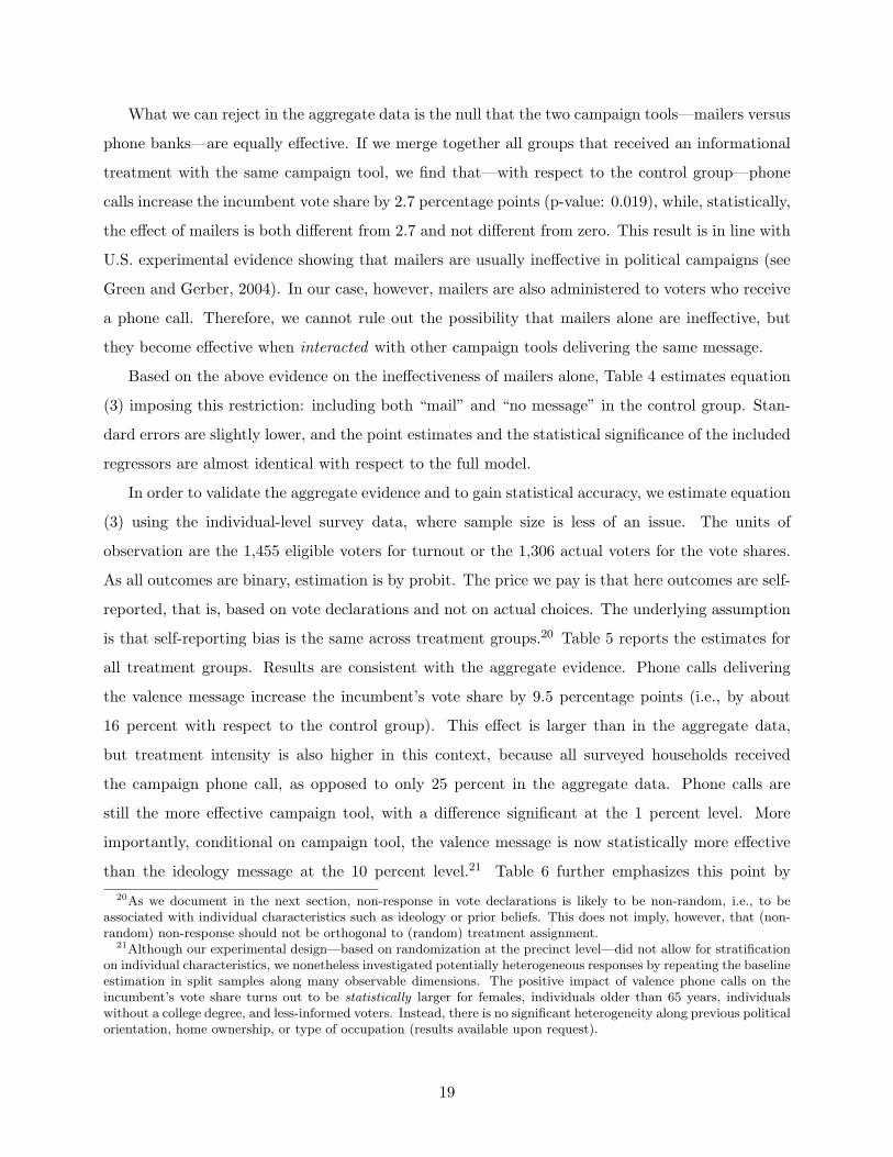
What we can reject in the aggregate data is the null that the two campaign tools—mailers versus

phone banks—are equally effective. If we merge together all groups that received an informational

treatment with the same campaign tool, we find that—with respect to the control group—phone

calls increase the incumbent vote share by 2.7 percentage points (p-value: 0.019), while, statistically,

the effect of mailers is both different from 2.7 and not different from zero. This result is in line with

U.S. experimental evidence showing that mailers are usually ineffective in political campaigns (see

Green and Gerber, 2004). In our case, however, mailers are also administered to voters who receive

a phone call. Therefore, we cannot rule out the possibility that mailers alone are ineffective, but

they become effective when interacted with other campaign tools delivering the same message.

Based on the above evidence on the ineffectiveness of mailers alone, Table 4 estimates equation

(3) imposing this restriction: including both “mail” and “no message” in the control group. Stan-

dard errors are slightly lower, and the point estimates and the statistical significance of the included

regressors are almost identical with respect to the full model.

In order to validate the aggregate evidence and to gain statistical accuracy, we estimate equation

(3) using the individual-level survey data, where sample size is less of an issue. The units of

observation are the 1,455 eligible voters for turnout or the 1,306 actual voters for the vote shares.

As all outcomes are binary, estimation is by probit. The price we pay is that here outcomes are self-

reported, that is, based on vote declarations and not on actual choices. The underlying assumption

is that self-reporting bias is the same across treatment groups.20 Table 5 reports the estimates for

all treatment groups. Results are consistent with the aggregate evidence. Phone calls delivering

the valence message increase the incumbent’s vote share by 9.5 percentage points (i.e., by about

16 percent with respect to the control group). This effect is larger than in the aggregate data,

but treatment intensity is also higher in this context, because all surveyed households received

the campaign phone call, as opposed to only 25 percent in the aggregate data. Phone calls are

still the more effective campaign tool, with a difference significant at the 1 percent level. More

importantly, conditional on campaign tool, the valence message is now statistically more effective

than the ideology message at the 10 percent level.21 Table 6 further emphasizes this point by20As we document in the next section, non-response in vote declarations is likely to be non-random, i.e., to be

associated with individual characteristics such as ideology or prior beliefs. This does not imply, however, that (non-random) non-response should not be orthogonal to (random) treatment assignment.

21Although our experimental design—based on randomization at the precinct level—did not allow for stratificationon individual characteristics, we nonetheless investigated potentially heterogeneous responses by repeating the baselineestimation in split samples along many observable dimensions. The positive impact of valence phone calls on theincumbent’s vote share turns out to be statistically larger for females, individuals older than 65 years, individualswithout a college degree, and less-informed voters. Instead, there is no significant heterogeneity along previous politicalorientation, home ownership, or type of occupation (results available upon request).

19

focusing on informational treatments administered by phone: campaigning on valence brings more

votes to the incumbent and to the party lists that support him, and these point estimates are

statistically larger than those of campaigning on ideology alone.

Finally, in Appendix Table A4, we evaluate the potential impact of spillovers across neighboring

precincts. As a counterpart to Table 5, we estimate the effects on voting choices of the average

treatment intensity for individuals voting in the same polling place, although they may belong to

different precincts and therefore treatment groups. If Assumption 1 (SUTVA) is met, we expect

these measures to have no impact on choices for treatments detected as ineffective in Table 5, and

to have a less significant impact for treatments detected as effective in Table 5. It is thus reassuring

that none of these spillover estimates is statistically different from zero.22

5 Model Estimation

We now report the results from the maximum likelihood (ML) estimation of our voting model. The

estimation procedure is straightforward and relies on fitting individual vote declarations, which—

in Section 4—we have shown to closely match actual vote outcomes.23 The specification selection

warrants some discussion, however.

Section 2 discussed non-response parameters [βA, βB], preference parameters [γ, ζ, χ], belief pa-

rameters [φP,2, φV,2, φP,3, φV,3, αP , αV , ρA, ρB], and the choice of a copula family [Independent;

Frank; FGM ]. Concerning the preference parameters, a large literature in political economics and

political science has emphasized preference heterogeneity, for instance in the case of distaste for

specific policy outcomes, such as inflation or unemployment.24 We can easily accommodate this

feature by allowing a different [γ, ζ, χ] vector for left-wing (L), centrist (C), and right-wing (R) vot-

ers. We can as well accommodate heterogeneity in the dependence structure of the beliefs [ρA, ρB]

by allowing them to differ for L, C, and R voters. Concerning the skewness of the marginal beliefs,

one can experiment with relaxing the simple [αP , αV ] to a more flexible [αP,2, αV,2, αP,3, αV,3], thus

22Notice that point estimates are not directly comparable with those in Table 5 because the regressors are no longerdummies but shares. Compared to the average values and standard deviations of the spillover shares, however, pointestimates are generally small, and—as expected—they are larger for the administration of the valence message byphone, because in those cases the shares also include treated voters for whom there exists a non-zero effect.

23The identification of the model is assessed through several rounds of Monte Carlo simulations. For given parametervalues we simulated individual votes and ensured that the estimation based on the simulated data converged to theoriginal structural values. Our likelihood function depends on a relatively small number of parameters. This allows fora fairly extensive search for global optima over the parametric space. We use the patternsearch algorithm of Matlabwith differing initial values. Repeating the optimization procedure consistently delivers identical global optima. Wealso employed a genetic algorithm (GA) global optimizer with a large initial population of 10, 000 values followed bya simplex search method using the GA values as initial values for the local optimizer. Both methods resulted in thesame estimates but the patternsearch algorithm converges faster in our environment.

24Among others, see Di Tella, MacCulloch, and Oswald (2001); Gerber and Lewis (2004).

20

allowing the extent of the skew to change with the variance. All these are testable parametric

constraints that can be assessed based on likelihood ratio tests. On the other hand, the choice of

the copula family requires a generalized likelihood ratio test approach, as the copula families we

consider are non-nested. The Vuong (1989) model selection test is appropriate for this purpose.

In Appendix Tables A5 and A6 we report the full set of model estimates for all the relevant

combinations of parametric and copula assumptions, which are pairwise tested in Appendix Tables

A7, A8, and A9 through likelihood ratio tests and Vuong tests (for the copula). According to the

tests, the preferred specification allows for heterogeneity in preference parameters along the voter’s

self-declared ideological stance, for independence between the ideological and valence dimensions

of both candidates, and for common [αP , αV ]. Thus, the preferred model specification estimates

θ = [βA, βB, {γz, ζz, χz}z=L,C,R , φP,2, φV,2, φP,3, φV,3, αP , αV ]. We report the ML estimates for this

model in Table 7.

We first note that the estimates of the probability of response (i.e., the probability of disclosing

one’s vote) are 0.76 and 0.99 for predicted votes for A (βA) and B (βB), respectively, and are very

precisely estimated. While we cannot reject the null that the probability of response is one for

voters that voted for B, we can strongly reject the null for voters that voted for A, which justifies

our choice of modeling non-random non-response.25 Interestingly, voters who are predicted to have

voted B are more likely to disclose their vote, contrary to the possible hypothesis that those who

voted for the winner (A) should be more willing to disclose their preference for the winner. This

result squares with the intuition of conservative voters in Tuscany being particularly assertive.

Generally, the preference parameters are estimated with precision. The parameter governing

the interaction between valence and ideology values for the voter, χ, is estimated to be a fairly

precise zero. Imposing χ = 0 clarifies the interpretation of γ as the relative weight in preferences

of valence (x′) to the weight of ideology (1− x′). Hence, γ = x′

1−x′ = 1 implies equal weights along

both dimensions and this is what we find for L and C voters. The weight on valence for R voters

is, however, much lower, around 27 percent, versus a 73 percent weight on ideology.

Concerning the curvature of the ideological loss function u (.), surprisingly, we find ζ < 1 for all

three types of voters, indicating increasing losses but at diminishing rates from policies further away

from the voter’s bliss point. This is in contrast with the standard assumption of ζ = 2, quadratic25As further evidence in support of the probability of disclosing one’s vote being non-random, we ran a probit

regression of a dummy indicating whether or not a vote was disclosed on the elicited posterior beliefs and voter’sideology. An F test strongly rejects the null hypothesis of no explanatory power and hence random non-response(p-value = 0.000). Interestingly, the stronger voters’ beliefs about the valence of either candidate, the more likelyvoters are to disclose their vote.

21

losses, for example. For centrist voters, ζ is actually estimated to be zero, although the estimate is

rather imprecise. With ζ = 0, the loss due to deviations from the voter’s bliss point is constant and

independent of the candidate’s policy.

The belief parameters are also precisely estimated for the most part. Interestingly, the specifi-

cation feeds back information which allows us to assess certain features of the survey design. The

model clearly captures an intermediate level of uncertainty between flat (s = 1) and degenerate pri-

ors (s = 4) for both valence and ideology. The on-the-mode probability mass, φV,3, is estimated at

around 0.40 for valence and the corresponding parameter for ideology, φP,3, is estimated at around

0.58. Hence, voters answering 2 to 5 to Q2 are more certain than having flat priors, but definitely

not sure about the candidate being at the mode (i.e., answer 1 to Q2). Along the valence dimen-

sion, voters do not perceive the distinction between “very uncertain” (s = 2) and “rather uncertain”

(s = 3) given that, at the estimated values, φV,3 = φV,2. However, along the ideology dimension,

“rather uncertain” does result in less dispersion in the marginal distribution. In addition, the an-

swers given to the skewness dimension seem to be important only along the ideological dimension,

where αP > 1/2, but not on the valence dimension where αV is not significantly different from 1/2,

indicating a symmetric partitioning of the off-mode probability mass.

Finally, concerning the choice of the copula and the estimates of the dependence parameters,

we note that, although both the FGM and Frank copula models have typically higher likelihood

values than under independence, the loss of parsimony of the model does not justify the additional

parameters according to the Vuong tests (see Appendix Table A9). This result occurs because we can

only estimate [ρA, ρB] very imprecisely, which can be easily rationalized. The parameters [ρA, ρB]

are essentially identified by voters that are: i) close to a change in their vote choice between A and

B; and ii) characterized by non-degenerate and non-flat beliefs along both the ideology and valence

dimensions. These joint restrictions substantially reduce the number of observations providing

useful identifying variation for estimating [ρA, ρB]. Notwithstanding the lack of precision, looking

at the signs of the estimated dependence parameters in Appendix Tables A5 and A6 is intriguing.

We generally find evidence of a positive association between left position and valence perceptions

for A driven by left-wing voters, and a positive association between right position and valence

perceptions for B driven by right-wing voters. More extreme positions appear to be correlated with

higher valence, in accordance with the theoretical results in Bernhardt et al. (2011). The Frank

copula is preferred over the FGM copula, although we cannot reject the null of equal fit.

The structural estimation has allowed us to fully recover all of the parameters necessary to

characterize the individual belief distributions. We proceed to the analysis of voters’ beliefs next.

22

6 Evidence on Beliefs

The effect of partisan ads on beliefs is interesting per se, and it can shed light on the robustness

of the impact of the same ads on voting choices, based on their mutual consistency. To increase

accuracy, we restrict our attention to informational treatments delivered by phone, that is, by

means of the effective campaign tool. In Tables 8 and 10, the outcomes are the average and the

standard deviation of the individual belief distributions—from model estimation—of both valence

and ideology of the incumbent and of the opponent, respectively. In Tables 9 and 11, we look at the

same moments of the individual belief distributions, but we instead use survey responses as opposed

to estimates from the structural model. Specifically, the outcomes are the (self-reported) mode and

a binary measure of “uncertainty” (namely, a dummy capturing flat priors in survey responses).

Estimation is by OLS for multivalued or continuous outcomes and by probit for binary outcomes.26

For the incumbent, both the valence and ideology messages have the expected direct effects.

Information on valence increases perceived competence by about 5 percent with respect to the

average perception. The same holds for information on ideology, as perceived ideology decreases

(i.e., moves to the left) by about 5 percent. Interestingly, second moments are also affected by the

two treatments: uncertainty about the incumbent’s valence or ideology is reduced by additional

campaign information along the corresponding dimension. Decreased uncertainty is a relevant

channel of the effect of campaign information on choices. As a matter of fact, the positive effect

of valence phone calls on the incumbent’s vote share is stronger in the subsample of voters whose

priors are flat. In the treated group, we observe a sharp tightening of the belief distribution, which

contributes to the overall effect.

The negative impact of ideology message phone calls on the candidate’s ideology does not trans-

late into more (or less) votes for A. Notwithstanding the large utility weight voters place on this

dimension, the shift in the belief distributions caused by the ideology phone calls is not strong

enough to affect voting choices.27

With respect to ideology, information on the incumbent’s position has interesting cross-effects

on the perception of the opponent’s position. Voters who received the ideology phone call from the

incumbent campaign move their subjective evaluation of the opponent B to the right by 3 percent.

The treatment also reduces uncertainty along this dimension. This might be due to the increased26For the sake of intuition, we use OLS also for the ideology mode, which can only take five (ordinal) values. Results

from ordered Probit are qualitatively identical (available upon request).27An alternative explanation might be that the ideology message affects right-wing and left-wing in the opposite

way, but this is not what we find in our sample. Ideology phone calls had negligible effects on voting behavior forboth types of voters, while their impact on beliefs was almost equivalent.

23

salience of the left/right distinction or to its relative nature, and it is causal evidence of cross-

learning between political campaigns. This finding is consistent with a sophisticated subjective

updating behavior on the part of the voters. For example, this type of evidence would be consistent

(albeit not proof of) Bayesian updating in a two-candidate signaling game.

7 Model Fit and Counterfactual Electoral Campaigns

To conclude our analysis we discuss model fit results and counterfactual electoral simulations based

on our structural estimates. Overall, the structural model under the baseline specification predicts

the actual vote correctly 88.7 percent of the time. In particular, we predict correctly 95.9 percent of

the votes for candidate A and 70.7 percent of the votes for B. Here, the sample under consideration

is restricted to the voters who disclosed their vote only, since we do not know the actual vote of

those who chose not to disclose it.

Turning to counterfactuals, no standard protocol exists in the literature for running these types

of exercises, so we have devised one. Suppose one wishes to assess what would have happened to

the aggregate vote share of A if everybody in the city had received the valence message (i.e., had

gotten treatment H = 1). We simulate this counterfactual campaign using a five step procedure.

Under our stability Assumption 6, for each voter i, it is possible to generate prior belief dis-

tributions about A and B based upon their prior survey answers and θ′, the structural parameter

vector estimated from votes and posterior beliefs. This is the first step. Secondly, for each voter

i ∈ T (h) with h 6= 1 (i.e., not treated with the valence message to begin with), it is always possible

to find the nearest neighbor treated match in the group h = 1, i′ ∈ T (1), based on the Mahalanobis

distance metric derived from covariates (such as age, gender, marital status, education, priors, and

ideology). Voter i′ is the closest match to voter i for which the causal effect of valence on beliefs

is actually observed. Essentially, this is the same intuition one would follow in propensity score

estimation. Once the closest match i′ has been identified, as third step we compute the difference

between i′’s marginal posterior and prior beliefs at every point of the support of each of the valence

and ideology dimensions. Fourth, we apply i′’s pointwise changes in beliefs to i’s priors to calculate

the counterfactual posterior marginal beliefs of i, under the assumption that, had i gotten the same

treatment as i′, she would have updated her beliefs in the same way as i′. Fifth, we compute joint

posterior beliefs using the appropriate copula family and the estimated ρ’s. Given the posteriors for

each voter i, we obtain a simulated electoral outcome, by calculating the expected utility of each

candidate for i and then predicting their vote for the candidate with the highest expected utility.

24

Importantly, this simulation procedure does not require the simulated electoral campaign to only

focus on a single treatment, but it can be tweaked to targeting specific subgroups with different

treatments. For instance, we can simulate a campaign in which valence messages are sent to

known centrist and right-wing voters while ideological messages are sent to left-wing voters. This

is of particular relevance at a point in time when political campaigns, especially in the US, have

increasingly turned to specialized companies, such as Aristotle, for micro data acquisition and

selective campaign advertising, a trend well under way also in commercial and online marketing.

We explore some of the possible electoral counterfactuals in Table 12. For each counterfactual, we

include all voters, even those who did not disclose their actual vote. Table 12 reports counterfactual

electoral outcomes for five types of campaigns by A: (1) a blanket valence campaign; (2) a blanket

ideological campaign; (3) a blanket double valence-ideology campaign; (4) a targeted campaign of

valence messages to center and right-wing voters and double messages to left-wing voters; (5) a

targeted campaign of ideological messages to center and right-wing voters and double messages

to left-wing voters. All results are benchmarked to the simulated electoral outcome that would

have realized in the absence of any campaign message on our part. The counterfactuals are also

assessed in their precision by constructing 95 percent asymptotic confidence intervals based on

bootstrapping from the asymptotic distribution of the parameters. All our counterfactual estimates

appear statistically precise.

The most effective possible campaign is the electoral campaign in which valence messages alone

are sent to all voters. A blanket valence campaign increases the vote share of A by 2.2 percentage

points relative to no campaign, which is more than enough to make the difference in a closely-

contested election. Interestingly, a blanket campaign of ideology messages actually reduces the

vote share of A substantially, in fact by the same 2.2 percentage points that a blanket valence

campaign would instead bring to A. In fact, the 95 percent confidence intervals for the two simulated

campaigns do not overlap, so we can be reasonably certain that a blanket valence campaign would

have outperformed a blanket ideology campaign. To understand why the ideology campaign reduces

vote shares, recall that the ideological message in our experiment has a leftist bent, reducing the

expected utility from A for R, C and possibly the most moderate of the L voters. Overall, the loss

of support from C and R in our sample turns out to more than sufficient to offset the gain in L

voters. For the same reason, a double campaign of both ideology and valence messages increases

the vote share of A by 0.5 percentage points, which, while effective, is not as effective as the blanket

valence-only campaign. Finally, the mixed campaign in which L voters get both types of messages

while C and R voters get valence messages only is almost as effective as the valence campaign,

25

while the campaign in which L voters get both types of messages while C and R voters get ideology

messages substantially decreases A’s vote share. In summary, consistently with our overall results,

campaigning on valence appeared the most effective tool to persuade voters.

8 Conclusion

This paper presents novel evidence on the effects of campaign information on voters’ decisions in

a large-scale field experiment. Importantly, our effects are observed both in vote declarations of

surveyed voters and in actual vote outcomes at the precinct level. To the best of our knowledge, this

is the first empirical randomization exercise in the literature that operates at the scale of an entire

election and covers the entire voting population in a mature democracy. Both our reduced-form

and structural estimation results uncover large electoral gains from valence-based informational

campaigning, possibly due to the relatively higher lack of prior information about the candidates

along this dimension.

An additional contribution of our paper is to present a belief elicitation protocol that allows us,

when combined with information on the electoral choices of voters, to completely characterize voters’

beliefs about candidates along both the ideological and valence dimensions. Our methodology allows

us to flexibly incorporate multivariate belief distributions within a structural random utility voting

model. We then employ this empirical model to structurally estimate both belief distributions and

voters’ preference parameters.

From a methodological viewpoint, we incorporate a general structure of beliefs updating that

goes well beyond what normally achievable with standard assumptions in the political and com-

mercial advertising literature. For instance, let us consider conjugate priors of the Gaussian family.

With normal beliefs new signals cannot reduce the precision of the subjective distributions, they

always reduce the variance of these distributions. But relying on such beliefs is very restrictive. To

see this consider another intuitive belief distribution: a binomial. When there are two (or more

generally finite) states, the probability of the “good” state can go up or down depending on the

signal value. As a result, the variance of the beliefs can actually increase or decrease after receiving

additional information. Hence, the importance of leaving the beliefs family unrestricted is crucial

in not forcing erroneous assumptions onto the data.

Our estimates show that the utility weight placed by voters on a candidate’s policy position is

of approximately equal magnitude to that placed on a candidate’s valence and that the common

assumption of convexity of the losses from ideological distance is not supported by the data. We

26

also show how the informational treatments we designed systematically influence both the first

and second moments of voters’ marginal beliefs about both candidates in the electoral race, not

only the beliefs about the candidate originating the message. We believe this causal evidence of

cross-campaign learning can prove useful for understanding the level of sophistication in subjective

updating by voters.

Potential applications of our elicitation methodology and estimation appear to be quite wide, in-

cluding, in addition to political campaigning, commercial advertising and marketing. Our approach

could be of use for the assessment of any type of informational treatment for randomized controlled

trials, most of them currently performed in developing countries. Finally, our incorporation of

the probability of non-response may be applied in many other contexts in which non-random non-

response to survey questions seems plausible (e.g., reports of income or other labor-related questions

for which those surveyed may be uncomfortable disclosing information).

27

References

[1] Ansolabehere, Stephen, and Shanto Iyengar. 1995. Going Negative: How Political Advertise-ments Shrink and Polarize the Electorate. New York: The Free Press.

[2] Ansolabehere, Stephen, Shanto Iyengar, Adam Simon, and Nicholas Valentino. 1994. “DoesAttack Advertising Demobilize the Electorate?” American Political Science Review, 88, 829–838.

[3] Ansolabehere, Stephen and James M. Snyder. 2000. “Valence Politics and Equilibrium in Spa-tial Election Models,”Public Choice, 103, 327–336.

[4] Ansolabehere, Stephen, James M. Snyder, and Charles Stewart, III. 2001. “Candidate Posi-tioning in U.S. House Elections,”American Journal of Political Science, 45, 136–159.

[5] Aragones, Enriqueta and Thomas R. Palfrey. 2002. “Mixed Equilibrium in a Downsian Modelwith a Favored Candidate,”Journal of Economic Theory, 103, 131–161.

[6] Ashworth, Scott and Ethan Bueno de Mesquita. 2009. “Elections with Platform and ValenceCompetition,” Games and Economic Behavior, 67, 191–216.

[7] Banerjee, Abhijit, Selvan Kumar, Rohini Pande, and Felix Su. 2011. “Do Informed Voters MakeBetter Choices? Experimental Evidence from Urban India,” MIT manuscript.

[8] Banerjee, Abhijit, Donald Green, and Rohini Pande. 2012. “Can Voters be Primed to ChooseBetter Legislators? Evidence from Voter Campaigns in India,” MIT manuscript.

[9] Bernhardt, Dan, Odilon Camara, and Francesco Squintani. 2011. “Competence and Ideology,”Review of Economic Studies, 78, 487–522.

[10] Blass, Asher A., Saul Lach, and Charles F. Manski. 2010. “Using Elicited Choice Probabili-ties to Estimate Random Utility Models: Preferences for Electricity Reliability,”InternationalEconomic Review, 51, 421–440.

[11] Chappell, Henry W. Jr. 1994. “Campaign Advertising and Political Ambiguity,” Public Choice,79, 281–303.

[12] Cox, David R. 1958. Planning of Experiments. New York: Wiley.

[13] Dewan, Torun, Macartan Humphreys, and Daniel Rubenson. 2010. “The Impact of Leadersand the Messages They Convey,” LSE manuscript.

[14] Di Tella, Rafael, Robert J. MacCulloch, and Andrew J. Oswald. 2001. “Preferences over Infla-tion and Unemployment: Evidence from Surveys of Happiness,”American Economic Review,91, 335–341.

[15] Dominitz, Jeff and Charles Manski. 1996. “Eliciting Student Expectations of the Returns toSchooling,” Journal of Human Resources, 31, 1–26.

[16] Duffy, John and Margit Tavits. 2008. “Beliefs and Voting Decisions: A Test of the PivotalVoter Model,” American Journal of Political Science, 52, 603–618.

28

[17] Enelow, James M. and Melvin J. Hinich. 1982. “Nonspatial Candidate Characteristics andElectoral Competition,” Journal of Politics, 44, 115–130.

[18] Farlie, Dennis J. 1960. “The Performance of Some Correlation Coefficients for a General Bi-variate Distribution,” Biometrika 47, 307–323.

[19] Fujiwara, Thomas and Leonard Wantchekon. 2013. “Can Informed Public Deliberation Over-come Clientelism? Experimental Evidence from Benin,” American Economic Journal: AppliedEconomics, forthcoming.

[20] Galasso, Vincenzo and Tommaso Nannicini. 2011. “Competing on Good Politicians,” AmericanPolitical Science Review, 105, 79–99.

[21] Garthwaite, Paul H., Joseph B. Kadane, and Anthony O’Hagan. 2005. “Statistical Methodsfor Eliciting Probability Distributions,” Journal of the American Statistical Association, 100,680–700.

[22] Gerber, Alan S., James G. Gimpel, Donald P. Green, and Daron Shaw. 2011. “How Largeand Long-lasting Are the Persuasive Effects of Televised Campaign Ads? Results from aRandomized Field Experiment,” American Political Science Review, 105, 135–150.

[23] Gerber, Alan S., and Donald P. Green. 2000. “The Effects of Canvassing, Telephone Calls, andDirect Mail on Voter Turnout: A Field Experiment,” American Political Science Review, 94,653–63.

[24] Gerber, Alan S., Donald P. Green, and Ron Shachar. 2003. “Voting May Be Habit-Forming:Evidence from a Randomized Field Experiment,” American Journal of Political Science, 47,540–50.

[25] Gerber Elisabeth R. and Jeffrey B. Lewis. 2004. “Beyond the Median: Voter Preferences,District Heterogeneity, and Political Representation,” Journal of Political Economy, 112, 1364–1383.

[26] Gill, Jeff and Lee D. Walker. 2005. “Elicited Priors for Bayesian Model Specifications in PoliticalScience Research,” Journal of Politics, 67, 841–872.

[27] Green, Donald P., and Alan S. Gerber. 2004. Get Out the Vote: How to Increase Voter Turnout.Washington, D.C.: Brookings Institution Press.

[28] Groseclose, Timothy. 2001. “A Model of Candidate Location When One Candidate Has aValence Advantage,”American Journal of Political Science, 45, 862–886.

[29] Kadane, Joseph and Lara J. Wolfson. 1998. “Experiences in Elicitation,” Journal of the RoyalStatistical Society, 47, 3–19.

[30] Kartik, Navin and R. Preston McAfee. 2007. “Signaling Character in Electoral Competi-tion,”American Economic Review, 97, 852–870.

[31] Lee, David, Enrico Moretti and Matthew J. Butler. 2004. “Do Voters Affect or Elect Policies?Evidence from the U.S. House,” Quarterly Journal of Economics, 119, 807–859.

[32] Liu, Scott and Patricia Stout. 1987. “Effects of Message Modality and Appeal on AdvertisingAcceptance,” Psychology and Marketing, 4, 167–87.

29

[33] Manski, Charles F. 2004 “Measuring Expectations,” Econometrica, 72, 1329–1376.

[34] Manski,Charles F. and Francesca Molinari. 2010. “Rounding Probabilistic Expectations inSurveys,” Journal of Business and Economic Statistics, 28, 219–231.

[35] Miller, George A. 1956. “The Magical Number Seven, Plus or Minus Two: Some Limits onOur Capacity for Processing Information,” Psychological Review 63, 81–97.

[36] Nickerson, David W. 2008. “Is Voting Contagious? Evidence from Two Field Experiments,”American Political Science Review, 102, 49–57.

[37] Ramalho, Esmeralda A. and Richard J. Smith. 2012. “Discrete Choice Nonresponse,” Reviewof Economic Studies, 7, 34–58.

[38] Rubin, Donald B. 1978. “Bayesian Inference for Causal Effects: The Role of Randomization,”The Annals of Statistics, 79, 1–20.

[39] Savage, Leonard. 1971. “Elicitation of Personal Probabilities and Expectations,” Journal of theAmerican Statistical Association, 66, 783–801.

[40] Schofield, Norman. 2003. “Valence Competition in the Spatial Stochastic Model,” Journal ofTheoretical Politics, 15, 371–383.

[41] Sklar Abe. 1959. “Fonctions de rı¿12partition ı¿1

2 n dimensions et leurs marges,” Publicationsde l’Institut de Statistique de l’Universitı¿1

2 de Paris, 8, 229–231.

[42] Stokes, Donald E. 1963. “Spatial Models of Party Competition,”American Political ScienceReview, 57, 368–377.

[43] Vicente, Pedro C. 2013. “Is Vote-buying Effective? Evidence from a Field Experiment in WestAfrica,” Economic Journal, forthcoming.

[44] Vuong, Quang H. 1989. “Likelihood Ratio Tests for Model Selection and Non-Nested Hypothe-ses,” Econometrica, 2, 307–333.

[45] Wantchekon, Leonard. 2003. “Clientelism and Voting Behavior: Evidence from a Field Exper-iment in Benin,” World Politics, 55, 399–422.

[46] Wattenberg, Martin P. and Craig L. Brians. 1999. “Negative Campaign Advertising: Demobi-lizer or Mobilizer?” American Political Science Review, 93, 891–899.

[47] Zafar, Basit. 2009. “College Major Choice and the Gender Gap,” Federal Reserve Bank of NewYork Staff Report No. 364.

30

Tables and Figures

Table 1 – Election Results at a Glance

Mean Median S.d. Min Max Obs.

Turnout 0.708 0.714 0.050 0.389 0.788 95

Incumbent shareover valid votes 0.513 0.508 0.061 0.354 0.667 95

Incumbent partiesover valid votes 0.541 0.542 0.065 0.358 0.679 95

Notes. Descriptive statistics at the precinct level of the variables specified in the first column. “In-cumbent parties” refer to the vote shares of the party lists supporting the incumbent.

Table 2 – Vote Declarations at the Individual Level

Mean Median S.d. Min Max Obs.

Declared turnout 0.898 1.000 0.303 0.000 1.000 1,455

Declared votefor the incumbent 0.571 1.000 0.495 0.000 1.000 1,306

Declared votefor incumbent parties 0.493 0.000 0.500 0.000 1.000 1,306

Notes. Descriptive statistics at the individual level of the variables specified in the first column.“Incumbent parties” refer to the (self-declared) vote in favor of the party lists supporting the incumbent.

31

Table 3 – Reduced-Form Aggregate Estimates, All Groups

Reference group: no messageValence Valence Ideology Ideology Double Double

by phone by mail by phone by mail by phone by mail

Turnout -0.011 -0.000 0.013 0.010 -0.006 -0.006[0.031] [0.015] [0.011] [0.013] [0.009] [0.013]

Incumbent 0.041** 0.004 0.013 0.021 0.027* -0.023share [0.019] [0.025] [0.016] [0.025] [0.015] [0.015]

Incumbent 0.032* 0.018 0.015 0.029 0.021 -0.015parties [0.018] [0.023] [0.016] [0.026] [0.014] [0.015]

Notes. Observations: 95 precincts. OLS coefficients reported; dependent variables in row headings and treatment groups incolumn headings. Robust standard errors clustered at the polling place level in brackets. Significance at the 10% level isrepresented by *, at the 5% level by **, and at the 1% level by ***.

Table 4 – Reduced-Form Aggregate Estimates, Phone Calls

Reference group: mail or no messageValence Ideology Double

by phone by phone by phone

Turnout -0.012 0.012 -0.006[0.030] [0.011] [0.010]

Incumbent 0.040** 0.012 0.026*share [0.019] [0.015] [0.013]

Incumbent 0.026 0.008 0.014parties [0.020] [0.016] [0.012]

Notes. Observations: 95 precincts. OLS coefficients reported; dependent variables in rowheadings and treatment groups in column headings. Robust standard errors clustered atthe polling place level in brackets. Significance at the 10% level is represented by *, atthe 5% level by **, and at the 1% level by ***.

32

Table 5 – Reduced-Form Individual Estimates, All Groups

Reference group: no messageValence Valence Ideology Ideology Double Double

by phone by mail by phone by mail by phone by mail

Turnout -0.024 -0.019 0.006 0.033 -0.019 -0.003[0.027] [0.034] [0.026] [0.022] [0.028] [0.029]

Incumbent 0.095** -0.061 0.018 -0.028 0.035 0.004share [0.039] [0.049] [0.049] [0.043] [0.050] [0.050]

Incumbent 0.109*** -0.007 -0.008 -0.044 0.009 -0.014parties [0.040] [0.060] [0.061] [0.046] [0.051] [0.049]

Notes. Observations: 1,455 eligible voters (turnout); 1,306 actual voters (vote shares). Probit marginal effects reported;dependent variables in row headings and treatment groups in column headings. Fixed effects for survey date included. Robuststandard errors clustered at the precinct level in brackets. Significance at the 10% level is represented by *, at the 5% level by**, and at the 1% level by ***.

Table 6 – Reduced-Form Individual Estimates, Phone Calls

Reference group: mail or no messageValence Ideology Double

by phone by phone by phone

Turnout -0.026 0.005 -0.021[0.023] [0.023] [0.023]

Incumbent 0.110*** 0.035 0.051share [0.033] [0.043] [0.045]

Incumbent 0.123*** 0.005 0.022parties [0.032] [0.053] [0.044]

Notes. Observations: 1,455 eligible voters (turnout); 1,306 actual voters (vote shares).Probit marginal effects reported; dependent variables in row headings and treatmentgroups in column headings. Fixed effects for survey date included. Robust standard errorsclustered at the precinct level in brackets. Significance at the 10% level is represented by*, at the 5% level by **, and at the 1% level by ***.

33

Table 7 – Model Estimates, Baseline Specification

Model’s Estimateparameters [s.e.]βA =Pr(response|A) 0.76

[0.01]βB =Pr(response|B) 0.99

[0.01]γL 1.08

[0.21]γC 1.10

[0.14]γR 0.37

[0.13]ζL 0.34

[0.21]ζC 0.00

[0.49]ζR 0.98

[0.32]χL 0.18

[0.14]χC 0.02

[0.09]χR -0.03

[0.05]φV,3 0.40

[0.15]φV,2 0.40

[0.28]αV 0.56

[0.05]φP,3 0.58

[0.16]φP,2 0.38

[0.19]αP 0.71

[0.19]Loglikelihood -1,043.60Observations 1,306Notes. Asymptotic standard errors in brackets. The selected speci-fication assumes independence of marginals, heterogeneous preferenceparameters, and forces same skew of marginal distribution of beliefsfor different stated levels of uncertainty.

34

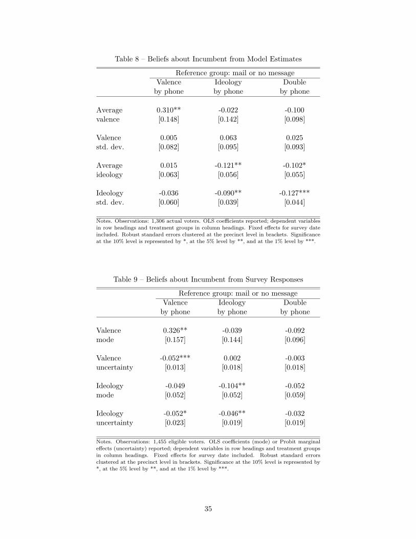
Table 8 – Beliefs about Incumbent from Model Estimates

Reference group: mail or no messageValence Ideology Double

by phone by phone by phone

Average 0.310** -0.022 -0.100valence [0.148] [0.142] [0.098]

Valence 0.005 0.063 0.025std. dev. [0.082] [0.095] [0.093]

Average 0.015 -0.121** -0.102*ideology [0.063] [0.056] [0.055]

Ideology -0.036 -0.090** -0.127***std. dev. [0.060] [0.039] [0.044]

Notes. Observations: 1,306 actual voters. OLS coefficients reported; dependent variablesin row headings and treatment groups in column headings. Fixed effects for survey dateincluded. Robust standard errors clustered at the precinct level in brackets. Significanceat the 10% level is represented by *, at the 5% level by **, and at the 1% level by ***.

Table 9 – Beliefs about Incumbent from Survey Responses

Reference group: mail or no messageValence Ideology Double

by phone by phone by phone

Valence 0.326** -0.039 -0.092mode [0.157] [0.144] [0.096]

Valence -0.052*** 0.002 -0.003uncertainty [0.013] [0.018] [0.018]

Ideology -0.049 -0.104** -0.052mode [0.052] [0.052] [0.059]

Ideology -0.052* -0.046** -0.032uncertainty [0.023] [0.019] [0.019]

Notes. Observations: 1,455 eligible voters. OLS coefficients (mode) or Probit marginaleffects (uncertainty) reported; dependent variables in row headings and treatment groupsin column headings. Fixed effects for survey date included. Robust standard errorsclustered at the precinct level in brackets. Significance at the 10% level is represented by*, at the 5% level by **, and at the 1% level by ***.

35

Table 10 – Beliefs about Opponent from Model Estimates

Reference group: mail or no messageValence Ideology Double

by phone by phone by phone

Average -0.127 -0.045 -0.071valence [0.081] [0.133] [0.094]

Valence -0.077 -0.096 -0.048std. dev. [0.110] [0.107] [0.132]

Average -0.075 0.189** -0.032ideology [0.067] [0.075] [0.070]

Ideology 0.041 -0.177*** -0.091std. dev. [0.075] [0.064] [0.057]

Notes. Observations: 1,306 actual voters. OLS coefficients reported; dependent variablesin row headings and treatment groups in column headings. Fixed effects for survey dateincluded. Robust standard errors clustered at the precinct level in brackets. Significanceat the 10% level is represented by *, at the 5% level by **, and at the 1% level by ***.

Table 11 – Beliefs about Opponent from Survey Responses

Reference group: mail or no messageValence Ideology Double

by phone by phone by phone

Valence -0.094 -0.043 -0.051mode [0.106] [0.133] [0.088]

Valence -0.028 -0.029 0.008uncertainty [0.047] [0.045] [0.054]

Ideology 0.023 0.141** -0.016mode [0.048] [0.062] [0.063]

Ideology -0.044 -0.089*** 0.001uncertainty [0.028] [0.030] [0.032]

Notes. Observations: 1,455 eligible voters. OLS coefficients (mode) or Probit marginaleffects (uncertainty) reported; dependent variables in row headings and treatment groupsin column headings. Fixed effects for survey date included. Robust standard errorsclustered at the precinct level in brackets. Significance at the 10% level is represented by*, at the 5% level by **, and at the 1% level by ***.

36

Table 12 – Predicted Vote Differences under Counterfactual Electoral Campaigns

Counterfactual treatment Predicted vote differencein percentage points

Blanket valence 2.2treatment [0.77, 3.33]

Blanket ideology -2.2treatment [-3.37, -0.27]

Blanket valence & ideology 0.5treatment [-0.73, 1.84]

Valence treatment to center & right 1.3valence & ideology to left voters [-0.19, 2.37]

Ideology treatment to center & right -2.4valence & ideology to left voters [-3.87, -0.92]

Actual electoral 1.8campaign effect [1.23, 3.14]

Notes. Counterfactual additional votes (in percentage points) that candidate A would have obtained withthe simulated campaigns described in the first column relative to no electoral treatment being administered.Bootstrapped 95 percent confidence intervals in brackets. Confidence intervals are based on 1,000 draws fromthe asymptotic distribution of the ML parameter vectors.

37

Figure 1 – Prior Valence Marginal Distribution for Voter #371

Figure 2 – Prior Joint Probability Distribution for Voter #369

38

Figure 3 – Posterior Joint Probability Distribution for Voter #369

39

Appendix

For all materials related to the design of our randomized controlled trial (including survey question-naires; colored treatment flyers; audio files of the treatment phone calls; and maps of the treatmentgroups) please refer to the website: www.igier.unibocconi.it/randomized-campaign.

In the next two subsections, we report the English translations of the text of the mail flyers (whichare then showed in Figure A1 and Figure A2) and of the text of the candidate’s recorded messagesfor the campaign phone calls.

In the subsection devoted to tables and figures, we report:

• balancing tests of precinct characteristics across treatment groups (Table A1);

• balancing tests of individual characteristics across treatment groups (Table A2);

• balancing tests of 2001 Census characteristics across treatment groups (Table A3);

• estimates of potential spillover effects (Table A4);

• complete summary of the structural model estimations (Tables A5 and A6);

• LR and Voung tests of model selection (Tables A7, A8, and A9);

• flyers for both the valence and ideology message (Figures A1 and A2).

A1 Mail Flyers: English Translations

Valence flyer. COMPETENCE AND EFFORT. 100 million worth of investments: Spent in parton the Fortress, squares, streets, and parking lots. PIUSS, the integrated plan for the development ofthe city: The city of Arezzo was ranked first in Tuscany; this is an important accomplishment. Inno-vation: The digital center, the hydrogen pipeline, and the energy house. FANFANI FOR MAYOR.

Ideology flyer. AWARENESS AND SOLIDARITY. Children: Created an integrated system tocater the needs of all, opened 3 new public nursery schools. Elderly: In-home assistance, new publicservices to help families. A network of solidarity for the neediest: Housing, meal centers, workintegration services. FANFANI FOR MAYOR.

A2 Phone Call Recorded Messages: English Translations

Valence message. Dear Voter, the 15th and 16th of May, the citizens of Arezzo will vote to electthe mayor and city councilmen. We all therefore have the opportunity to make an informed choicefor the future of Arezzo. Over the last years, my administration invested 100 million Euros todevelop and improve our city. Results are under the eyes of everyone and can be observed by simplylooking at the Fortress, the squares, the streets, and the parking lots. Thanks to the quality of our

40

work, the PIUSS—the plan for the development of the city of Arezzo—was ranked first among thosein Tuscany. This was an important accomplishment that also enabled us to gain access to importantfinancial resources to improve the prominence of our city. However, we did much more than this,we strived to boost innovation with the digital center, the hydrogen pipeline, and the energy house.Given also all these reasons, I take the liberty to ask for your vote in the election of the 15th and16th of May. Reward our COMPETENCE and our EFFORT. Best regards from Giuseppe Fanfani.

Ideology message. Dear Voter, the 15th and 16th of May, the citizens of Arezzo will vote to electthe mayor and city councilmen. We all will have the opportunity to make an informed choice for thefuture of Arezzo. For us, future stands for SOLIDARITY. In these five years of city government, wedealt with issues regarding childhood creating an integrated system of services able to provide answersto all families and opening three new public nursery schools. We also took care of our elderly people,providing new services to help families assist them and increasing in-home assistance. At the sametime, we definitely did not forget about those that found themselves living in difficult circumstancesalso because they were affected by the international crisis that severely struck our region. In fact, weincreased housing, meal centers, and professional integration services for all those in need. Givenalso all these reasons, I take the liberty to ask for your vote in the election of the 15th and 16thof May. Make SOLIDARITY win! For an “Arezzo” careful and open to the hardships of those inneed. Best regards from Giuseppe Fanfani.

Valence plus ideology message. Dear Voter, the 15th and 16th of May, the citizens of Arezzowill vote to elect the mayor and city councilmen. We all therefore have the opportunity to makean informed choice for the future of Arezzo. Over the last years, my administration invested 100million Euros to develop and improve our city. Results are under the eyes of everyone and canobserved by simply looking at the Fortress, the squares, the streets, and the parking lots. Thanksto the quality of our work, the PIUSS—the plan for the development of the city of Arezzo—wasranked first among those in Tuscany. At the same time, we definitely did not forget about those thatfound themselves living in difficult circumstances also because they were affected by the internationalcrisis that severely struck our region. In fact, we increased housing, meal centers, and professionalintegration services for all those in need. Given also all these reasons, I take the liberty to askfor your vote in the election of the 15th and 16th of May. Reward our COMPETENCE and ourEFFORT. Make SOLIDARITY win! For an Arezzo careful and open to the hardships of those inneed. Best regards from Giuseppe Fanfani.

41

Appendix Tables and Figures

Table A1 – Ex-Ante Balancing Tests at the Precinct Level

Reference group: no messageValence Valence Ideology Ideology Double Double

by phone by mail by phone by mail by phone by mail

Eligible voters -66.083 -101.583 19.250 -63.667* -65.500 -6.083[96.591] [70.235] [57.771] [36.922] [66.886] [56.033]

First neighborhood 0.036 0.036 0.203 -0.047 0.203 -0.047[0.136] [0.112] [0.178] [0.112] [0.123] [0.109]

Second neighborhood 0.116 -0.051 -0.051 -0.051 -0.051 0.033[0.188] [0.140] [0.151] [0.154] [0.086] [0.128]

Third neighborhood -0.014 0.236 -0.098 0.152 -0.014 -0.098[0.190] [0.172] [0.134] [0.199] [0.169] [0.134]

Fourth neighborhood -0.138 -0.221 -0.054 -0.054 -0.138 0.112[0.149] [0.141] [0.146] [0.164] [0.139] [0.129]

Regional ’10 turnout -0.005 -0.003 0.016 0.012 0.000 -0.002[0.025] [0.016] [0.010] [0.010] [0.010] [0.014]

Regional ’10 left 0.011 0.013 0.013 0.012 0.004 -0.021[0.015] [0.019] [0.013] [0.017] [0.013] [0.013]

Regional ’10 right -0.015 -0.017 0.011 0.007 -0.006 0.019[0.015] [0.014] [0.012] [0.018] [0.011] [0.018]

European ’09 turnout -0.004 0.008 0.019 0.013 0.002 0.007[0.026] [0.012] [0.012] [0.013] [0.011] [0.012]

European ’09 left -0.012 0.015 -0.016 -0.014 0.018 -0.028[0.030] [0.026] [0.016] [0.025] [0.019] [0.021]

European ’09 right 0.009 -0.015 0.018 0.009 -0.014 0.026[0.022] [0.021] [0.015] [0.024] [0.020] [0.020]

National ’08 turnout -0.014 0.012 0.002 0.002 0.005 0.000[0.025] [0.008] [0.006] [0.007] [0.007] [0.009]

National ’08 left 0.016 0.026 -0.015 -0.004 0.020 -0.019[0.019] [0.019] [0.019] [0.028] [0.020] [0.017]

National ’08 right -0.018 -0.023 0.013 0.004 -0.024 0.023[0.020] [0.017] [0.017] [0.028] [0.021] [0.018]

City ’06 turnout -0.002 0.008 0.012 0.009 0.011 -0.006[0.020] [0.011] [0.009] [0.013] [0.011] [0.013]

City ’06 left 0.016 0.035 -0.029 -0.017 0.009 -0.029[0.029] [0.024] [0.023] [0.034] [0.021] [0.022]

City ’06 right -0.014 -0.037 0.028 0.014 -0.008 0.022[0.029] [0.024] [0.022] [0.033] [0.021] [0.024]

Notes. Observations: 95 precincts, 86 (European), 84 (National), 83 (City). OLS coefficients reported; dependent variables inrow headings and treatment groups in column headings. Eligible voters is the number of eligible voters in the precinct (average820.168). The neighborhood dummies capture the city-wide neighborhood the precinct belongs to. The other variables are theelectoral outcomes in past elections and are expressed as vote shares. Robust standard errors clustered at the polling place levelin brackets. Significance at the 10% level is represented by *, at the 5% level by **, and at the 1% level by ***.

42

Table A2 – Ex-Post Balancing Tests at the Individual Level

Reference group: no messageValence Valence Ideology Ideology Double Double

by phone by mail by phone by mail by phone by mail

Male 0.008 0.014 0.034 0.004 0.006 0.042[0.039] [0.050] [0.038] [0.038] [0.047] [0.039]

Over 65 -0.035 0.004 -0.012 0.086 -0.046 0.056[0.053] [0.048] [0.048] [0.053] [0.042] [0.048]

College -0.004 -0.027 0.010 0.008 0.035 -0.016graduate [0.035] [0.041] [0.041] [0.047] [0.045] [0.040]

Out of -0.019 0.010 -0.037 0.048 -0.041 0.050labor force [0.052] [0.054] [0.058] [0.059] [0.050] [0.053]

White 0.029 -0.005 0.032 -0.013 0.008 -0.013collar [0.045] [0.043] [0.038] [0.041] [0.039] [0.038]

Other -0.010 -0.005 0.006 -0.035 0.033 -0.037occupation [0.049] [0.041] [0.040] [0.039] [0.042] [0.051]

Center-left 0.045 0.058 -0.009 -0.033 -0.059 0.014[0.044] [0.055] [0.048] [0.040] [0.042] [0.059]

Home owner -0.017 -0.007 -0.045 0.027 0.007 -0.037[0.040] [0.030] [0.039] [0.036] [0.033] [0.028]

Read 0.037 -0.007 0.025 -0.024 0.032 0.048the press [0.036] [0.038] [0.042] [0.052] [0.049] [0.047]

Watch TV 0.034 -0.016 0.038 0.068 -0.033 0.055[0.042] [0.055] [0.039] [0.046] [0.042] [0.038]

Notes. Observations: 1,455 eligible voters. OLS coefficients reported; dependent variables in row headings and treatment groupsin column headings. All variables are dummies. Read the press and Watch TV capture whether the voter declares to do this“very often” or “often.” Fixed effects for survey date included. Robust standard errors clustered at the precinct level in brackets.Significance at the 10% level is represented by *, at the 5% level by **, and at the 1% level by ***.

43

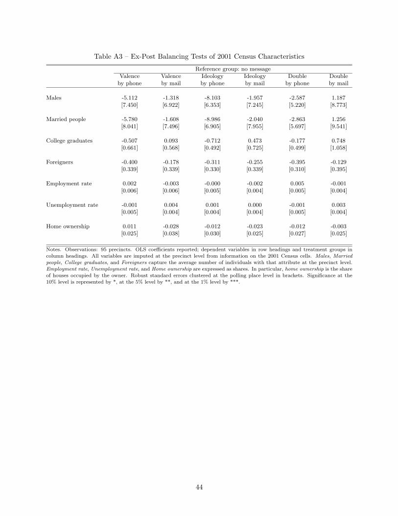
Table A3 – Ex-Post Balancing Tests of 2001 Census Characteristics

Reference group: no messageValence Valence Ideology Ideology Double Double

by phone by mail by phone by mail by phone by mail

Males -5.112 -1.318 -8.103 -1.957 -2.587 1.187[7.450] [6.922] [6.353] [7.245] [5.220] [8.773]

Married people -5.780 -1.608 -8.986 -2.040 -2.863 1.256[8.041] [7.496] [6.905] [7.955] [5.697] [9.541]

College graduates -0.507 0.093 -0.712 0.473 -0.177 0.748[0.661] [0.568] [0.492] [0.725] [0.499] [1.058]

Foreigners -0.400 -0.178 -0.311 -0.255 -0.395 -0.129[0.339] [0.339] [0.330] [0.339] [0.310] [0.395]

Employment rate 0.002 -0.003 -0.000 -0.002 0.005 -0.001[0.006] [0.006] [0.005] [0.004] [0.005] [0.004]

Unemployment rate -0.001 0.004 0.001 0.000 -0.001 0.003[0.005] [0.004] [0.004] [0.004] [0.005] [0.004]

Home ownership 0.011 -0.028 -0.012 -0.023 -0.012 -0.003[0.025] [0.038] [0.030] [0.025] [0.027] [0.025]

Notes. Observations: 95 precincts. OLS coefficients reported; dependent variables in row headings and treatment groups incolumn headings. All variables are imputed at the precinct level from information on the 2001 Census cells. Males, Marriedpeople, College graduates, and Foreigners capture the average number of individuals with that attribute at the precinct level.Employment rate, Unemployment rate, and Home ownership are expressed as shares. In particular, home ownership is the shareof houses occupied by the owner. Robust standard errors clustered at the polling place level in brackets. Significance at the10% level is represented by *, at the 5% level by **, and at the 1% level by ***.

44

Table A4 – Evaluating Potential Spillovers, All Groups

Reference group: no messageValence Valence Ideology Ideology Double Double

by phone by mail by phone by mail by phone by mailspillovers spillovers spillovers spillovers spillovers spillovers

Turnout 0.032 -0.034 0.010 0.047 0.003 0.028[0.048] [0.055] [0.044] [0.060] [0.042] [0.054]

Incumbent 0.099 -0.113 0.064 -0.020 0.124 0.005share [0.077] [0.082] [0.080] [0.100] [0.076] [0.099]

Incumbent 0.081 -0.147 -0.035 -0.118 0.038 0.006parties [0.079] [0.098] [0.096] [0.104] [0.089] [0.115]

Notes. Observations: 1,455 eligible voters (turnout); 1,306 actual voters (vote shares). OLS coefficients reported; dependentvariables in row headings and treatment groups in column headings. Each spillovers variable captures the share of observationswho received the corresponding treatment in the same polling place of every observation. Average values are: 0.135 (valence byphone); 0.099 (valence by mail); 0.151 (ideology by phone); 0.106 (ideology by mail); 0.135 (double by phone); 0.113 (double bymail). Fixed effects for survey date included. Robust standard errors clustered at the precinct level in brackets. Significance atthe 10% level is represented by *, at the 5% level by **, and at the 1% level by ***.

45

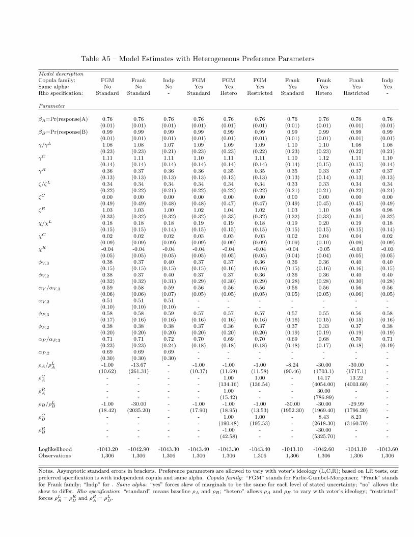
Table A5 – Model Estimates with Heterogeneous Preference Parameters

Model descriptionCopula family: FGM Frank Indp FGM FGM FGM Frank Frank Frank IndpSame alpha: No No No Yes Yes Yes Yes Yes Yes YesRho specification: Standard Standard - Standard Hetero Restricted Standard Hetero Restricted -

Parameter

βA=Pr(response|A) 0.76 0.76 0.76 0.76 0.76 0.76 0.76 0.76 0.76 0.76(0.01) (0.01) (0.01) (0.01) (0.01) (0.01) (0.01) (0.01) (0.01) (0.01)

βB=Pr(response|B) 0.99 0.99 0.99 0.99 0.99 0.99 0.99 0.99 0.99 0.99(0.01) (0.01) (0.01) (0.01) (0.01) (0.01) (0.01) (0.01) (0.01) (0.01)

γ/γL 1.08 1.08 1.07 1.09 1.09 1.09 1.10 1.10 1.08 1.08(0.23) (0.23) (0.21) (0.23) (0.23) (0.22) (0.23) (0.23) (0.22) (0.21)

γC 1.11 1.11 1.11 1.10 1.11 1.11 1.10 1.12 1.11 1.10(0.14) (0.14) (0.14) (0.14) (0.14) (0.14) (0.14) (0.15) (0.15) (0.14)

γR 0.36 0.37 0.36 0.36 0.35 0.35 0.35 0.33 0.37 0.37(0.13) (0.13) (0.13) (0.13) (0.13) (0.13) (0.13) (0.14) (0.13) (0.13)

ζ/ζL 0.34 0.34 0.34 0.34 0.34 0.34 0.33 0.33 0.34 0.34(0.22) (0.22) (0.21) (0.22) (0.22) (0.22) (0.21) (0.21) (0.22) (0.21)

ζC 0.00 0.00 0.00 0.00 0.00 0.00 0.00 0.00 0.00 0.00(0.49) (0.49) (0.48) (0.48) (0.47) (0.47) (0.49) (0.45) (0.45) (0.49)

ζR 1.03 1.03 1.00 1.02 1.04 1.02 1.03 1.10 0.98 0.98(0.33) (0.32) (0.32) (0.32) (0.33) (0.32) (0.32) (0.33) (0.31) (0.32)

χ/χL 0.18 0.18 0.18 0.19 0.19 0.18 0.19 0.20 0.19 0.18(0.15) (0.15) (0.14) (0.15) (0.15) (0.15) (0.15) (0.15) (0.15) (0.14)

χC 0.02 0.02 0.02 0.03 0.03 0.03 0.02 0.04 0.04 0.02(0.09) (0.09) (0.09) (0.09) (0.09) (0.09) (0.09) (0.10) (0.09) (0.09)

χR -0.04 -0.04 -0.04 -0.04 -0.04 -0.04 -0.04 -0.05 -0.03 -0.03(0.05) (0.05) (0.05) (0.05) (0.05) (0.05) (0.04) (0.04) (0.05) (0.05)

φV,3 0.38 0.37 0.40 0.37 0.37 0.36 0.36 0.36 0.40 0.40(0.15) (0.15) (0.15) (0.15) (0.16) (0.16) (0.15) (0.16) (0.16) (0.15)

φV,2 0.38 0.37 0.40 0.37 0.37 0.36 0.36 0.36 0.40 0.40(0.32) (0.32) (0.31) (0.29) (0.30) (0.29) (0.28) (0.28) (0.30) (0.28)

αV /αV,3 0.59 0.58 0.59 0.56 0.56 0.56 0.56 0.56 0.56 0.56(0.06) (0.06) (0.07) (0.05) (0.05) (0.05) (0.05) (0.05) (0.06) (0.05)

αV,2 0.51 0.51 0.51 - - - - - - -(0.10) (0.10) (0.10) - - - - - - -

φP,3 0.58 0.58 0.59 0.57 0.57 0.57 0.57 0.55 0.56 0.58(0.17) (0.16) (0.16) (0.16) (0.16) (0.16) (0.16) (0.15) (0.15) (0.16)

φP,2 0.38 0.38 0.38 0.37 0.36 0.37 0.37 0.33 0.37 0.38(0.20) (0.20) (0.20) (0.20) (0.20) (0.20) (0.19) (0.19) (0.19) (0.19)

αP /αP,3 0.71 0.71 0.72 0.70 0.69 0.70 0.69 0.68 0.70 0.71(0.23) (0.23) (0.24) (0.18) (0.18) (0.18) (0.18) (0.17) (0.18) (0.19)

αP,2 0.69 0.69 0.69 - - - - - - -(0.30) (0.30) (0.30) - - - - - - -

ρA/ρLA -1.00 -13.67 - -1.00 -1.00 -1.00 -8.24 -30.00 -30.00 -

(10.62) (261.31) - (10.37) (11.69) (11.58) (90.46) (1703.1) (1717.1) -ρC

A - - - - 1.00 1.00 - 14.17 13.22 -- - - - (134.16) (136.54) - (4054.00) (4003.60) -

ρRA - - - - 1.00 - - 30.00 - -

- - - - (15.42) - - (786.89) - -ρB/ρL

B -1.00 -30.00 - -1.00 -1.00 -1.00 -30.00 -30.00 -29.99 -(18.42) (2035.20) - (17.90) (18.95) (13.53) (1952.30) (1969.40) (1796.20) -

ρCB - - - - 1.00 1.00 - 8.43 8.23 -

- - - - (190.48) (195.53) - (2618.30) (3160.70) -ρR

B - - - - -1.00 - - -30.00 - -- - - - (42.58) - - (5325.70) - -

Loglikelihood -1043.20 -1042.90 -1043.30 -1043.40 -1043.30 -1043.40 -1043.10 -1042.60 -1043.10 -1043.60Observations 1,306 1,306 1,306 1,306 1,306 1,306 1,306 1,306 1,306 1,306

Notes. Asymptotic standard errors in brackets. Preference parameters are allowed to vary with voter’s ideology (L,C,R); based on LR tests, ourpreferred specification is with independent copula and same alpha. Copula family: “FGM” stands for Farlie-Gumbel-Morgensen; “Frank” standsfor Frank family; “Indp” for . Same alpha: “yes” forces skew of marginals to be the same for each level of stated uncertainty; “no” allows theskew to differ. Rho specification: “standard” means baseline ρA and ρB ; “hetero” allows ρA and ρB to vary with voter’s ideology; “restricted”forces ρL

A = ρRB and ρR

A = ρLB .

Table A6 – Model Estimates without Heterogeneous Preference Parameters

Model descriptionCopula family: FGM Frank Indp FGM FGM FGM Frank Frank Frank IndpSame alpha: No No No Yes Yes Yes Yes Yes Yes YesRho specification: Standard Standard - Standard Hetero Restricted Standard Hetero Restricted -

Parameter

βA =Pr(response|A) 0.77 0.77 0.77 0.77 0.77 0.77 0.77 0.77 0.77 0.77(0.01) (0.01) (0.01) (0.01) (0.01) (0.01) (0.01) (0.01) (0.01) (0.01)

βB =Pr(response|B) 0.98 0.98 0.98 0.98 0.98 0.98 0.98 0.98 0.98 0.98(0.01) (0.01) (0.01) (0.01) (0.01) (0.01) (0.01) (0.01) (0.01) (0.01)

γ/γL 0.89 0.91 0.90 0.88 0.88 0.90 0.91 0.91 0.91 0.89(0.09) (0.09) (0.09) (0.09) (0.09) (0.09) (0.09) (0.09) (0.09) (0.09)

γC - - - - - - - - - -- - - - - - - - - -

γR - - - - - - - - - -- - - - - - - - - -

ζ/ζL 0.65 0.68 0.69 0.69 0.68 0.65 0.66 0.66 0.68(0.14) (0.14) (0.14) (0.14) (0.14) (0.14) (0.14) (0.14) (0.14) (0.14)

ζC - - - - - - - - - -- - - - - - - - - -

ζR - - - - - - - - - -- - - - - - - - - -

χ/χL 0.05 0.06 0.05 0.04 0.04 0.05 0.06 0.06 0.06 0.05(0.05) (0.05) (0.05) (0.05) (0.05) (0.05) (0.05) (0.05) (0.05) (0.05)

χC - - - - - - - - - -- - - - - - - - - -

χR - - - - - - - - - -- - - - - - - - - -φV,3 0.40 0.35 0.35 0.34 0.40 0.34 0.34 0.34 0.34 0.34

(0.17) (0.16) (0.15) (0.15) (0.17) (0.17) (0.16) (0.16) (0.16) (0.16)φV,2 0.40 0.35 0.35 0.34 0.40 0.34 0.34 0.34 0.34 0.34

(0.30) (0.29) (0.29) (0.24) (0.30) (0.25) (0.28) (0.29) (0.29) (0.28)αV /αV,3 0.54 0.54 0.54 0.51 0.52 0.52 0.52 0.52 0.52 0.52

(0.07) (0.06) (0.06) (0.05) (0.06) (0.05) (0.05) (0.05) (0.05) (0.05)αV,2 0.50 0.50 0.50 - - - - - - -

(0.11) (0.10) (0.10) - - - - - - -φP,3 0.60 0.58 0.61 0.65 0.65 0.60 0.61 0.58 0.62 0.65

(0.17) (0.15) (0.15) (0.17) (0.17) (0.15) (0.16) (0.15) (0.15) (0.15)φP,2 0.60 0.55 0.61 0.65 0.65 0.60 0.61 0.58 0.61 0.65

(0.33) (0.32) (0.32) (0.27) (0.28) (0.26) (0.26) (0.27) (0.26) (0.26)αP /αP,3 0.80 0.77 0.81 0.81 0.82 0.77 0.77 0.74 0.77 0.81

(0.26) (0.23) (0.27) (0.28) (0.28) (0.22) (0.23) (0.20) (0.23) (0.27)αP,2 0.69 0.65 0.70 - - - - - - -

(0.42) (0.35) (0.44) - - - - - - -ρA/ρL

A -1.00 -30.00 - -1.00 -1.00 1.00 -30.00 -30.00 29.99 -(18.09) (1993.00) - (22.79) (38.48) (24.90) (2120.70) (3038.50) (2786.20) -

ρCA - - - - 1.00 1.00 - 30.00 29.60 -

- - - - (53.29) (41.32) - (1849.70) (7268.40) -ρR

A - - - - -1.00 - - -30.00 - -- - - - (41.50) - - (2997.90) - -

ρB/ρLB 1.00 29.99 - 1.00 -1.00 -1.00 29.99 -30.00 -30.00 -

(29.21) (1633.70) - (37.36) (51.93) (22.23) (3674.60) (4066.60) (2467.70) -ρC

B - - - - 1.00 1.00 - 22.42 27.94 -- - - - (86.81) (63.35) - (6915.90) (11627.00) -

ρRB - - - - -1.00 - - -30.00 - -

- - - - (81.43) - - (7895.00) - -

Loglikelihood -1057.70 -1057.40 -1057.70 -1057.90 -1057.94 -1057.70 -1057.50 -1057.50 -1057.40 -1057.90Observations 1,306 1,306 1,306 1,306 1,306 1,306 1,306 1,306 1,306 1,306

Notes. Asymptotic standard errors in brackets. Unlike Table A3, preference parameters are not allowed to vary with voter’s ideology (L,C,R);based on LR tests, these are not our preferred specifications but we report them for completeness. Copula family: “FGM” stands for Farlie-Gumbel-Morgensen; “Frank” stands for Frank family; “Indp” for . Same alpha: “yes” forces skew of marginals to be the same for each level ofstated uncertainty; “no” allows the skew to differ. Rho specification: “standard” means baseline ρA and ρB ; “hetero” allows ρA and ρB to varywith voter’s ideology; “restricted” forces ρL

A = ρRB and ρR

A = ρLB .

Table A7 – LR Tests: Restriction of Preference ParametersTo Be the Same across Voter’s Ideology

Copula Test statistic P-value

FGM 28.94 0.00Frank 28.86 0.00Independent 28.62 0.00

Notes. Skew restricted to be the same across levels of stated uncertainty. Standard ρ specification.

Table A8 – LR Tests: Restriction of SkewTo Be the Same across Levels of Uncertainty

Preferences Copula Test statistic P-value

Homogeneous FGM 0.29 0.86Homogeneous Frank 0.37 0.83Homogeneous Indp 0.38 0.83Heterogeneous FGM 0.49 0.78Heterogeneous Frank 0.39 0.82Heterogeneous Indp 0.54 0.76

Notes. Standard ρ specification.

Table A9 – Vuong Tests: Copula Comparisons

Preferences Copula Rho Test P-value Preferredcomparison specification statistic copula

Homogeneous Frank vs. FGM Standard 0.76 0.45 FrankHomogeneous Independent vs. FGM Standard 39.48 0.00 IndependentHomogeneous Independent vs. Frank Standard 17.93 0.00 IndependentHeterogeneous Frank vs. FGM Standard 1.05 0.29 FrankHeterogeneous Independent vs. FGM Standard 22.67 0.00 IndependentHeterogeneous Independent vs. Frank Standard 12.61 0.00 IndependentHeterogeneous Independent vs. FGM Heterogeneous 52.08 0.00 IndependentHeterogeneous Independent vs. Frank Heterogeneous 26.59 0.00 IndependentHomogeneous Independent vs. FGM Heterogeneous 12.9 0.00 IndependentHomogeneous Independent vs. Frank Heterogeneous 35.93 0.00 IndependentHeterogeneous Independent vs. FGM Restricted 37.19 0.00 IndependentHeterogeneous Independent vs. Frank Restricted 30.78 0.00 IndependentHomogeneous Independent vs. FGM Restricted 40.57 0.00 IndependentHomogeneous Independent vs. Frank Restricted 34.77 0.00 Independent

Notes. Skew restricted to be the same across level of stated uncertainty.

48

Figure A1 – Campaign Flyer with the Valence Message

Figure A2 – Campaign Flyer with the Ideology Message

49