Embed Size (px)
Citation preview

How Do Incumbents Respond to the Threat of Entry? Evidence from the Major Airlines*
Austan Goolsbee University of Chicago, GSB
American Bar Foundation and NBER [email protected]
and
Chad Syverson University of Chicago
and NBER [email protected]
Original Draft: May 2004
Current Draft: December 2004
Abstract
This paper examines how incumbents respond to the threat of entry of competitors, as distinguished from their response to competitors’ actual entry. It uses a case study from the passenger airline industry—specifically, the evolution of Southwest Airlines’ route network—to identify particular routes where the probability of future entry rises abruptly. When Southwest begins operating in airports on both sides of a route but not the route itself, this dramatically raises the chance they will start flying that route in the near future. We examine the pricing of the incumbents on threatened routes in the period surrounding such events. We find that incumbents cut fares significantly when threatened by Southwest’s entry into their routes. This is true even after controlling in several ways for airport-specific operating costs. The response of incumbents seems to be limited only to the threatened route itself, and not to routes out of nearby competitor airports where Southwest does not operate (e.g., fares drop on routes from Chicago Midway but not Chicago O’Hare). The largest responses appear to be restricted to routes that were concentrated beforehand. Incumbents do experience short-run increases in their passenger loads concurrent with these fare cuts. This is consistent with theories implying incumbents will try to generate some longer-term loyalty among current customers before the entry of a new competitor. We examine evidence relating this demand-building motive to frequent flyer programs and find suggestive evidence in favor of this notion. There is only weak evidence that incumbents increase capacity on the routes. ________________________ * We thank Severin Borenstein, Dennis Carlton, Robert Gordon, Mara Lederman, Chris Mayer, Nancy Rose, Fiona Scott Morton, and seminar participants at the University of Chicago, Dartmouth (Tuck), the Minneapolis Federal Reserve Bank, MIT, Wharton, Wisconsin, Yale, the Society for Economic Dynamics Annual Meeting, the HBS Strategy Conference and the joint Federal Reserve Bank-GWU seminar for helpful comments. Luis Andres provided superior research assistance. Financial support from the NET Institute (http://www.NETinst.org) is gratefully acknowledged. Goolsbee wishes to thank the National Science Foundation for financial support as well.
I. Introduction
In this paper we examine how incumbents respond to the threat of entry by a competitor.
Though this topic has been the object of considerable theoretical and policy debate, it has
received little empirical attention, mainly due to the problems of identifying when the threat of
entry rises (as contrasted with when entry occurs, which is directly observable).
We will examine this issue in the passenger airline industry. In this circumstance, we are
able to identify discrete shifts in the threat of entry. We do this by using the expansion patterns
the most famous potential competitor in the industry, Southwest Airlines, to identify
circumstances where the threat of Southwest entering a specific route rises significantly.1
Specifically, we look at situations where Southwest begins operating in the second endpoint
airport of a route (having already been operating out of the first endpoint), but before it starts
flying the route itself. We investigate how incumbents’ prices respond to such threats. Since
major incumbent carriers have extensive route networks (offering many possible entry episodes)
and the government reports extensive fare data on these routes, we have considerable empirical
variation with which to identify any effects.
As an example of our empirical strategy, consider the recent entry of Southwest airlines
into the Philadelphia airport (this specific case is not in our data because it occurred so recently,
but it illustrates the episodes we study). On May 9, 2004, Southwest began operations in the
Philadelphia airport (PHL) with nonstop flights to six other cities in its network, and one-stop
service to several others. One route Southwest did not offer service when they entered the
Philadelphia market was Philadelphia-Jacksonville, Florida (JAX). Jacksonville is a Southwest
airport. Southwest does fly between JAX and other airports, just not PHL-JAX. Once
Southwest is operating out of both end points on a route—here both JAX and PHL—the
probability that they will soon start flying the route between those two airports goes up
dramatically. Indeed, operating in both end points raises the probability of entering the route by
nearly a factor of 60 in the data presented in a later section. With that increase in probability, we
can then look at, say, US Airways’ and United Airlines’ (the incumbents) fares on the JAX-PHL
route once Southwest threatens entry but has yet to actually start flying.
The paper builds on two literatures. Empirically, it is obviously connected to the
1 Southwest’s network has been expanding rapidly for some time and the impact of their actual entry on prices in a market is well known (see, for example, Morrison, 2001).
1

extensive literature on airline competition, especially the work relating to airport presence and
the sources of airport market power.2 These papers, however, have looked, almost exclusively,
at the impact of actual actions rather than pre-emptive actions. Our empirical strategy is perhaps
closest to Ellison and Ellison’s (2000) study of incumbent drug makers’ actions in the period just
preceding expiration of their patents.
The paper’s second connection is to the considerable body of theoretical work on
strategic entry deterrence, particularly those models that offer rationale for incumbents initiating
competitive actions before entry actually occurs. These include, for example, Dixit’s (1979)
capacity commitment motivation, the strategic learning-by-doing of Spence (1981), cost-
signaling as in Milgrom and Roberts (1982), the long-term contracting environment of Aghion
and Bolton (1987), and switching costs as in Klemperer (1987). These rationale were forwarded
as responses to the theoretical results implying that preemptive incumbent actions are irrational,
either because they are not subgame perfect (in the spirit of Selten’s (1978) chain-store paradox),
or because costly competitive actions should be delayed until entry actually occurs. These
papers counter the traditional argument that firms should act only when they actually face
competition. Our empirical work tests between the two views.
The results show that incumbents do respond to the threat of entry, quite separately from
their responses to actual entry. Incumbents drop average fares substantially when Southwest
threatens a route but before Southwest actually enters the route. This is true even when we
compare the fare changes on threatened routes to those on incumbents’ other routes out of the
same airports, indicating that shifts in airport-specific operating cost are not creating spurious
results. As expected, the lower prices increase in the number of passengers flying the
incumbents prior to entry. We also find, interestingly, that while incumbents cut fares on the
threatened route, they do not cut prices on routes to nearby airports in the same market (e.g.,
Chicago-O'Hare when Southwest threatens a Chicago-Midway route). Further, fare cuts are
considerably larger on routes that were concentrated before Southwest’s threat. There is only
weak evidence that airlines expand flight or seat capacity in response to the threat of entry;
instead, this additional demand is taken up mostly through higher load factors. Finally, we find
2 See, for example, Reiss and Spiller (1989), Hurdle et al. (1989), Borenstein (1989, 1991, 1992), Berry (1990, 1992), Brueckner et al. (1992), Evans and Kessides (1993), Whinston and Collins (1992), Borenstein and Rose (1994), Hendricks et al. (1997), and the more recent work of Bamberger, Carlton, and Neumann (2001) or Mayer and Sinai (2004).
2

suggestive evidence consistent with airlines trying to increase customer loyalty through
mechanisms like frequent flyer programs. The fare drops are greatest for incumbents’ high-fare-
paying customers and on routes with more business travelers.
II. Data
Because we are primarily concerned with fares, we use the U.S. Department of
Transportation’s DB1A files from 1993 to 2002 to build the core of our sample. These data
provide a 10% sample of all domestic tickets used in each quarter, which we use to compute the
average, standard deviation, and specific quantiles of logged ticket prices within each route-
carrier-quarter combination (unfortunately the data do not report any specific travel dates within
the quarter).3 Following the previous literature, we define a route by its two endpoint airports
alone, not any intermediate stops along the way. We look at so-called “direct flights”
(predominantly nonstop flights but technically including itineraries where the passenger stops
but does not change planes). We restrict our sample to routes between airports that Southwest
ever flies any flights to in our sample. This includes 838 routes between 61 different airports.
The “threatened” entry events we study are identified from the observed expansion
patterns of Southwest Airlines. Southwest grew tremendously throughout our sample period. Its
revenues grew from $2.3 billion to $5.5 billion, passenger-miles from 18.8 to 45.4 billion, and it
added service to 21 new airports between the end of 1993 and the start of 2003.4 Every time
Southwest begins service in a new airport, it raises the threat that Southwest will enter routes
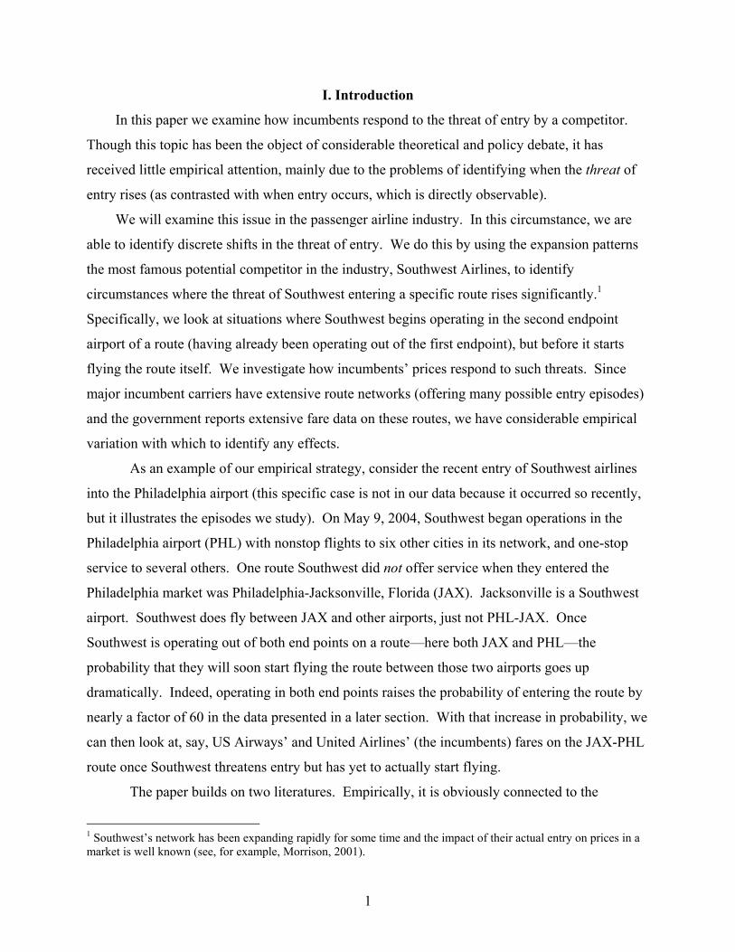
connecting that airport with other airports in its network. We illustrate this in Figure 1.
Southwest enters Philadelphia and begins flights from there to Tampa in the second quarter of
2004. Southwest is already flying out of Jacksonville (and has been since 1997) to cities in its
network other than Philadelphia. Now, though, the entry into Philadelphia makes Southwest
highly likely to start flying Philadelphia-Jacksonville in the near future.5
The importance of airport presence is well known in the industry as an indicator of future
3 We use Severin Borenstein’s cleaned files , which are aggregated up to the route-carrier-quarter level, since this is the level of our analysis rather than the ticket. We use the original source files to compute the fare quantiles since that information is not included in the Borenstein files. 4 Southwest exited one airport, San Francisco International (SFO), in 2001. It had operated there since before 1993. 5 Indeed, Southwest eventually did enter the PHL-JAX route in the fourth quarter of 2004. Our empirical specification captures the separate impacts of both such threatened-entry and actual-entry events.
3
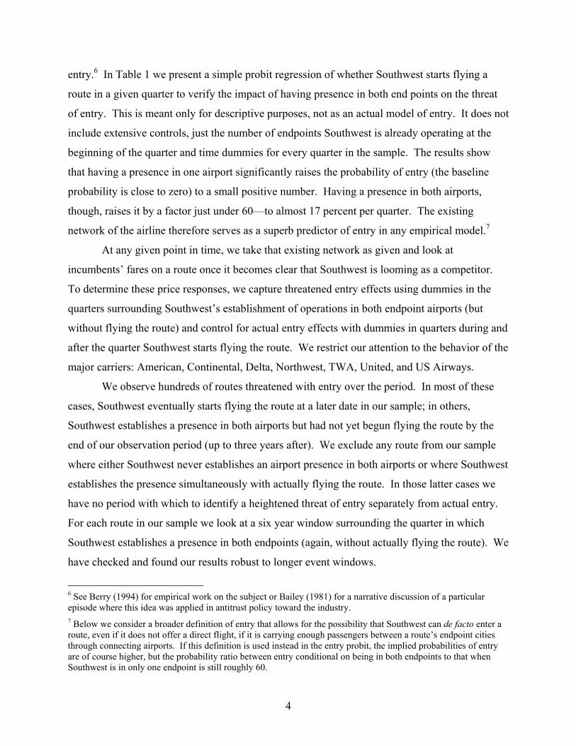
entry.6 In Table 1 we present a simple probit regression of whether Southwest starts flying a
route in a given quarter to verify the impact of having presence in both end points on the threat
of entry. This is meant only for descriptive purposes, not as an actual model of entry. It does not
include extensive controls, just the number of endpoints Southwest is already operating at the
beginning of the quarter and time dummies for every quarter in the sample. The results show
that having a presence in one airport significantly raises the probability of entry (the baseline
probability is close to zero) to a small positive number. Having a presence in both airports,
though, raises it by a factor just under 60—to almost 17 percent per quarter. The existing
network of the airline therefore serves as a superb predictor of entry in any empirical model.7
At any given point in time, we take that existing network as given and look at
incumbents’ fares on a route once it becomes clear that Southwest is looming as a competitor.
To determine these price responses, we capture threatened entry effects using dummies in the
quarters surrounding Southwest’s establishment of operations in both endpoint airports (but
without flying the route) and control for actual entry effects with dummies in quarters during and
after the quarter Southwest starts flying the route. We restrict our attention to the behavior of the
major carriers: American, Continental, Delta, Northwest, TWA, United, and US Airways.
We observe hundreds of routes threatened with entry over the period. In most of these
cases, Southwest eventually starts flying the route at a later date in our sample; in others,
Southwest establishes a presence in both airports but had not yet begun flying the route by the
end of our observation period (up to three years after). We exclude any route from our sample
where either Southwest never establishes an airport presence in both airports or where Southwest
establishes the presence simultaneously with actually flying the route. In those latter cases we
have no period with which to identify a heightened threat of entry separately from actual entry.
For each route in our sample we look at a six year window surrounding the quarter in which
Southwest establishes a presence in both endpoints (again, without actually flying the route). We
have checked and found our results robust to longer event windows.
6 See Berry (1994) for empirical work on the subject or Bailey (1981) for a narrative discussion of a particular episode where this idea was applied in antitrust policy toward the industry. 7 Below we consider a broader definition of entry that allows for the possibility that Southwest can de facto enter a route, even if it does not offer a direct flight, if it is carrying enough passengers between a route’s endpoint cities through connecting airports. If this definition is used instead in the entry probit, the implied probabilities of entry are of course higher, but the probability ratio between entry conditional on being in both endpoints to that when Southwest is in only one endpoint is still roughly 60.
4

We define Southwest's actual entry as occurring when it establishes direct service (i.e.,
flights without a change of plane) between the two airports. This definition of entry is easiest to
understand, but we will also show that the results are not sensitive to defining Southwest’s entry
as including cases where they start either direct or indirect service (involving a stop and a plane
change) on the route.8
In all, we observe Southwest threatening entry into 838 routes over the sample period.9
We focus on the behavior of major airline incumbents in the 25 quarters surrounding the initial
threat (that is, the three years before and the quarter that Southwest starts operating in the second
endpoint of the route, as well as the three years after). This yields almost 19,000 route-carrier-
quarter observations of average logged fares and passenger counts for major airlines’ direct
flights on threatened routes. Summary statistics for these variables are shown in Table 2.
III. Hypotheses and Empirical Specifications
Our baseline model measures the impact of Southwest establishing a presence in both
endpoints of a route by looking at the periods before, during, and after this event, while
controlling for other influences. The basic specification, with some slight abuse of summation
notation as explained below, is as follows:
0
3 3
, ,8 0
( _ _ _ ) ( _ _ )eri t ri t r t r t ri t ri ty SW in both airports SW flying route Xτ τ τ
τ τ, , ,τγ µ β δ α
+ +
+ +=− =
= + + + + +∑ ∑ ε , (1)
where yri,t is the outcome of interest (e.g., mean logged fares or logged total passengers) for
incumbent carrier i flying route r in quarter t. 0,_ _ _ r tSW in both airports τ+ are time dummies
surrounding the period when Southwest establishes a presence in both endpoints of a route but
before they have actually started flying the route. ,_ _er tSW flying route τ+ are time dummies
starting with the period Southwest actually starts flying on the route. Each dummy is mutually
exclusive of the others, so the implied effects on the dependent variable given by their
coefficients are not additive. The γri and µt are fixed effects for carrier-route and time. Some
specifications will also include a set of controls Xri,t.
8 Note that just because Southwest flies routes that could be connected does not mean that they operate a route indirectly. There are many routes where Southwest operates in both airports but they will not sell a single itinerary between the two and there are no tickets for the route in our sample. 9 By the final quarter of 2002 (the end of our observation period), Southwest had actually entered about 500 of these routes.
5
In all regressions, we weight observations by the number of passengers flying the route-
carrier in the quarter, so larger incumbent routes have a greater impact on the measured average
response than do smaller routes. We also cluster standard errors at the route level to account for
any correlation in unobservables across carriers or time periods within routes.
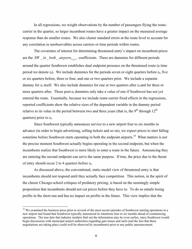
The covariates of interest for determining threatened entry’s impact on incumbent prices
are the 0,_ _ _ r tSW in both airports τ+ coefficients. There are dummies for different periods
around the quarter Southwest establishes dual endpoint presence on the threatened route (a time
period we denote t0). We include dummies for the periods seven or eight quarters before t0, five
or six quarters before, three or four, and one or two quarters prior. We include a separate
dummy for t0 itself. We also include dummies for one or two quarters after t0 and for three or
more quarters after. These post-t0 dummies only take a value of one if Southwest has not yet
entered the route. Essentially, because we include route-carrier fixed effects in the regressions,
reported coefficients show the relative sizes of the dependent variable in the dummy period
relative to its value in the period between two and three years (that is, the 9th through 12th
quarters) prior to t0.
Since Southwest typically announces service to a new airport four to six months in
advance (in order to begin advertising, selling tickets and so on), we expect prices to start falling
sometime before Southwest starts operating in both the endpoint airports.10 What matters is not
the precise moment Southwest actually begins operating in the second endpoint, but when the
incumbents realize that Southwest is more likely to enter a route in the future. Announcing they
are entering the second endpoint can serve the same purpose. If true, the price due to the threat
of entry should occur 2 to 4 quarters before t0.
As discussed above, the conventional, static-model view of threatened entry is that
incumbents should not respond until they actually face competition. This notion, in the spirit of
the classic Chicago-school critiques of predatory pricing, is based on the seemingly simple
proposition that incumbents should not cut prices before they have to. To do so entails losing
profits in the short-run and has no impact on profits in the future. This view implies that the
10 We examined the business press prior to several of the most recent episodes of Southwest starting operations in a new airport and found that Southwest typically announced its intentions four to six months ahead of commencing operations. The true date that industry insiders find out the information may be even earlier, since Southwest would begin discussions with municipal airport authorities regarding gate leases and such (and the fact that these negotiations are taking place could well be observed by incumbents) prior to any public announcement.
6

coefficients on the threat of entry should be zero.
However, three alternatives that might rationalize preemptive incumbent reactions. They
all have to do with dynamic effects. They are: reducing costs in the presence of learning-by-
doing, signaling, and generating some kind of long-term customer loyalty.
The first of these implies that when the industry technology involves learning by doing,
an incumbent firm facing the threat of entry may want to overproduce (in the sense that it will set
prices lower and sell more output than would be implied by the static game alone) so that in the
future, when the potential competitor would seek to enter, it will be a lower-cost and tougher
competitor. While such strategic considerations may be important in other industries, we do not
find learning-by-doing plausible here. The incumbents in our industry have all been operating
for decades and scale economies seem dubious.
Second, incumbent airlines could deter Southwest’s entry by signaling that they have low
costs on the route or are particularly committed to dominating the route, as in the spirit of, say,
Milgrom and Roberts (1982). Our view is that this, too, does not fit this industry well. Through
publicly available data sets (like the ones we use in this paper) airlines can observe a large share
of their competitors’ total costs and demand conditions such as capital stock attributes (planes’
ages, fuel consumptions, and carrying capacities), labor costs, load factors, etc. They also have
public knowledge of labor negotiations as well as gate lease agreements signed with public
airport authorities. Moreover, Southwest has entered these same incumbents’ routes dozens of
times, so one would expect they would already have a solid idea of the credibility and type of
their rivals. Though one can always devise a signaling model to explain the behavior we
observe, a priori, it seems a bit of a stretch in this case.11
A third and we think more plausible alternative is that incumbents’ fare cuts before
Southwest enters create some longer term loyalty among their customers. Such a mechanism
would introduce a dynamic element to demand. By locking in a customer base before actual
entry occurs, the major carriers could dampen the competitive impact of Southwest’s actual entry
if and when it does occur, similar to the idea of using long-term contracts as a barrier to entry as
in Aghion and Bolton (1987), or when there are switching costs inherent in changing to another
11 More subtle theories of signaling might involve things like incumbents signaling their willingness to protect a threatened route because it provides important connecting services to passengers or because the route is a “signature” route of the carrier. However, we do not see any way to test for these possibilities against the more straight forward story given the available data.
7

provider, as discussed in Klemperer (1987). The airline industry even has an straightforward
mechanism in place—frequent flyer programs—that induces just this sort of dynamic demand
behavior, and such issues have been discussed in work such as Cairns and Galbraith (1990),
Borenstein (1996), and Lederman (2004). Anything that might generate long term loyalty
through early price cutting would suffice, however.
IV. Baseline Empirical Results
Table 3 presents the results from estimating specification (1) using the average logged
fares on incumbent carriers’ routes faced with the threat of entry by Southwest. Column 1
presents the baseline specification where Southwest’s actual entry is defined as occurring when it
starts direct flights between the two cities. To document that the prices are not arising from
indirect competition from Southwest connecting flights, column 2 classifies Southwest entry into
a route as either when it starts direct flight service or when at least 40 passengers fly between the
route’s endpoints via change-of-plane service. For a one-in-ten sample, this restricts the sample
to routes that a passenger flies on Southwest at least around once per month.12 The number of
observations falls with change-of-plane entry definition because we look only at routes where
Southwest establishes a presence on both sides at least one quarter before they actually start
flying the route and with the broader definition of entry, there are more routes where Southwest
enters immediately.
There is a clear and statistically significant drop in prices at just the time the incumbent
learns that the threat of Southwest entry has increased. In the period well before, prices show no
significant trend. The coefficients on the periods 5 to 6 quarters before and 7 to 8 quarters before
Southwest establishes dual presence show no significant difference from the baseline period
preceding them (recall that the coefficients show the value of average logged fares relative to the
excluded period, i.e., the 9th through 12th quarters before Southwest establishes a dual endpoint
presence). Then, as Southwest’s entry into the second endpoint airport gets closer, prices begin
to fall rapidly. By 3 to 4 quarters before operating both endpoints of a route, incumbents’ fares
12 We check results using this broader entry definition because passengers could theoretically use connecting flights from the newly-entered endpoint airport to fly Southwest between city pairs even if direct flights are unavailable. We impose the 40-passenger-per-quarter threshold for the indirect-flights to count as entry in order to avoid counting weather diversions and things of that nature as entry as well as to exclude routes where connections are available but so inconvenient as to be rarely used. The estimates were basically identical having a threshold of zero or having a larger threshold.
8
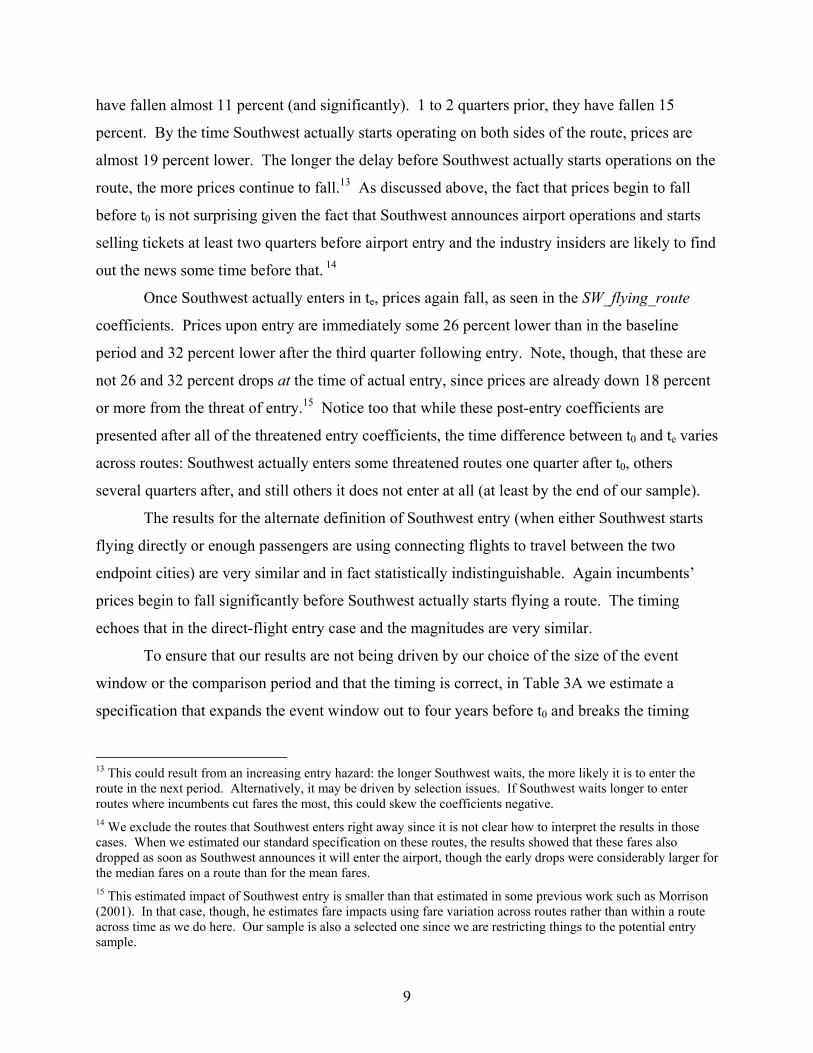
have fallen almost 11 percent (and significantly). 1 to 2 quarters prior, they have fallen 15
percent. By the time Southwest actually starts operating on both sides of the route, prices are
almost 19 percent lower. The longer the delay before Southwest actually starts operations on the
route, the more prices continue to fall.13 As discussed above, the fact that prices begin to fall
before t0 is not surprising given the fact that Southwest announces airport operations and starts
selling tickets at least two quarters before airport entry and the industry insiders are likely to find
out the news some time before that. 14
Once Southwest actually enters in te, prices again fall, as seen in the SW_flying_route
coefficients. Prices upon entry are immediately some 26 percent lower than in the baseline
period and 32 percent lower after the third quarter following entry. Note, though, that these are
not 26 and 32 percent drops at the time of actual entry, since prices are already down 18 percent
or more from the threat of entry.15 Notice too that while these post-entry coefficients are
presented after all of the threatened entry coefficients, the time difference between t0 and te varies
across routes: Southwest actually enters some threatened routes one quarter after t0, others
several quarters after, and still others it does not enter at all (at least by the end of our sample).
The results for the alternate definition of Southwest entry (when either Southwest starts
flying directly or enough passengers are using connecting flights to travel between the two
endpoint cities) are very similar and in fact statistically indistinguishable. Again incumbents’
prices begin to fall significantly before Southwest actually starts flying a route. The timing
echoes that in the direct-flight entry case and the magnitudes are very similar.
To ensure that our results are not being driven by our choice of the size of the event
window or the comparison period and that the timing is correct, in Table 3A we estimate a
specification that expands the event window out to four years before t0 and breaks the timing
13 This could result from an increasing entry hazard: the longer Southwest waits, the more likely it is to enter the route in the next period. Alternatively, it may be driven by selection issues. If Southwest waits longer to enter routes where incumbents cut fares the most, this could skew the coefficients negative. 14 We exclude the routes that Southwest enters right away since it is not clear how to interpret the results in those cases. When we estimated our standard specification on these routes, the results showed that these fares also dropped as soon as Southwest announces it will enter the airport, though the early drops were considerably larger for the median fares on a route than for the mean fares. 15 This estimated impact of Southwest entry is smaller than that estimated in some previous work such as Morrison (2001). In that case, though, he estimates fare impacts using fare variation across routes rather than within a route across time as we do here. Our sample is also a selected one since we are restricting things to the potential entry sample.
9
dummies out quarter-by-quarter (the excluded period is therefore the 15th and 16th quarters before
t0). The results confirm the baseline findings. From 16 quarters before all the way to 5 quarters
before, there is little pattern in prices and certainly none of the coefficients is significant. At
exactly the period we believe the incumbents learn that Southwest is going to establish a
presence on both sides of a route, prices begin to fall significantly. They drop by more than 12
percent over the three quarters.16
These basic results, then, suggest that incumbents are quite responsive to the threat of
Southwest entry. At least half—and perhaps as much as three-quarters—of the total impact of
Southwest airlines on incumbents’ fares occurs before Southwest actually enters a route. This
pre-entry impact is driven by Southwest threatening entry by announcing and establishing a
presence in the second endpoint airport on a route.
V. Testing for Plausibility and Controlling for Alternatives
A. The Number Passengers
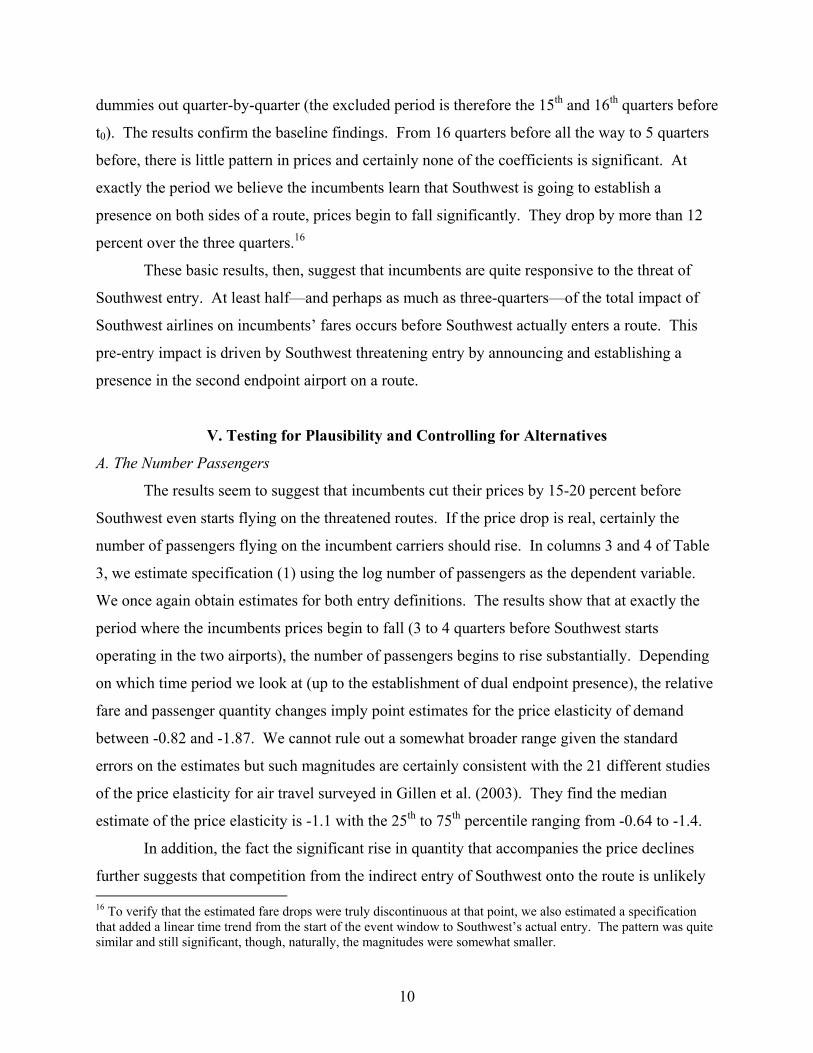
The results seem to suggest that incumbents cut their prices by 15-20 percent before
Southwest even starts flying on the threatened routes. If the price drop is real, certainly the
number of passengers flying on the incumbent carriers should rise. In columns 3 and 4 of Table
3, we estimate specification (1) using the log number of passengers as the dependent variable.
We once again obtain estimates for both entry definitions. The results show that at exactly the
period where the incumbents prices begin to fall (3 to 4 quarters before Southwest starts
operating in the two airports), the number of passengers begins to rise substantially. Depending
on which time period we look at (up to the establishment of dual endpoint presence), the relative
fare and passenger quantity changes imply point estimates for the price elasticity of demand
between -0.82 and -1.87. We cannot rule out a somewhat broader range given the standard
errors on the estimates but such magnitudes are certainly consistent with the 21 different studies
of the price elasticity for air travel surveyed in Gillen et al. (2003). They find the median
estimate of the price elasticity is -1.1 with the 25th to 75th percentile ranging from -0.64 to -1.4.
In addition, the fact the significant rise in quantity that accompanies the price declines
further suggests that competition from the indirect entry of Southwest onto the route is unlikely 16 To verify that the estimated fare drops were truly discontinuous at that point, we also estimated a specification that added a linear time trend from the start of the event window to Southwest’s actual entry. The pattern was quite similar and still significant, though, naturally, the magnitudes were somewhat smaller.
10

to be the source of the price declines. With pre-emption they are trying to increase passengers
today to improve demand post-entry. With competition, the demand for the incumbent should be
falling.
B. Comparisons and Cost Controls
In Table 4, we also consider the potential role of cost shocks as an alternative explanation
for the results. In particular, if Southwest chooses to enter airports that it knows will experience
positive operating cost shocks in the near future, this will lead to a spurious correlation between
our measure of Southwest's threat of entry and the subsequent decline in incumbents’ fares.
To control for such cost shocks we first, in columns 2 and 3, compare the fares on a
threatened route to a control group of the carrier’s fares on other routes involving the same
airports on one end but non-Southwest airports on the other (column 1 reports again the baseline
price regression from Table 3). We illustrate the principle behind the routes in the control
groups in Figure 2. In the Philadelphia-Jacksonville example, the dependent variable in column
2 is the average logged fare on (say) US Airways’ PHL-JAX route minus the average logged
fares on US Airways’ routes between PHL and airports to which Southwest doesn’t fly (we
restrict alternative airports to those in the top 100 to be comparable). We do the same in column
3, but now for routes between JAX and non-Southwest airports. The regressions look at what
happens to incumbents’ prices on a threatened route relative to their prices on their other routes
out of the same airports. Any airport-specific operating cost shocks should expectedly be
removed from this relative fare difference. The coefficients here are even larger than before. By
the time Southwest establishes dual presence on the route, the incumbent’s prices fall 20 to 24
percent relative to their prices on other routes out of those same airports.
In column 4, we go a step further and include those alternative-route prices directly in the
regression as explanatory variables. (The average fares on the control routes are referred to as
the “operating cost controls” in the table.) These controls have significant and positive
coefficients, as one would expect. When US Airways’ fares rise on routes between Jacksonville
and other airports, US Airways’ fares also rise on the threatened route out of Jacksonville. The
estimated impact of Southwest's threat, however, is virtually unchanged with the addition of
these cost controls. Whereas we previously found incumbent fares down about 19 percent by the
time Southwest establishes airport presence on both sides of a route, here we find them down
11

about 18 percent (and not significantly different from before).
These tests indicate that fare drops on threatened routes are not merely reflecting fare
declines in all routes out of the endpoint airports. Instead, the fare reductions documented in the
baseline results seem independent of overall fare movements.
C. Concentrated Routes
Of course, incumbent routes vary in their market structure even before Southwest
threatens to enter. Some are highly concentrated, while on others incumbents face a great deal of
competition. Previous work on the airline industry has suggested that the concentrated routes are
places the incumbents may have market power whereas the routes with many competitors may
be effectively competitive already. If true, we would expect to find a larger impact of the entry
threat from Southwest on routes with higher concentration.
To get at this issue, we split our sample by the HHI of carriers on that particular route
over the four quarters prior to Southwest’s entry threat. Column 1 of Table 5 shows the
estimates from our baseline price regression obtained using routes whose HHI is at the median or
below. Column 2 shows results from routes above the median. The results show that prices only
decline on the concentrated routes. On low HHI routes, incumbents’ prices have fallen only
about 2 percent by the time Southwest begins operating in the second endpoint airport, and this
estimate is not significantly different from zero. On the high HHI routes, on the other hand, fares
have dropped more than 20 percent and the coefficients are very significant.
D. Behavior in “Nearby” Airports
In some large metropolitan areas, Southwest establishes its airport presence in one of the
area’s secondary airports. Our results above look at incumbent responses out of the Southwest
airport itself, but we also want to examine cases where the incumbent operates out of a “nearby”
airport that might compete with the Southwest airport. To do so we will look specifically at
incumbent prices on routes flying out of LaGuardia, JFK, and Newark airports (when Southwest
threatens entry into routes from Islip, Long Island), Miami (Southwest: Ft. Lauderdale), Reagan-
National and Washington-Dulles (Southwest: BWI), Boston (Southwest: Providence and
Manchester) and Chicago O’Hare (Southwest: Midway). We must exclude the Los Angeles, San
Francisco, Houston and Dallas markets from this regression because, during our sample period,
12
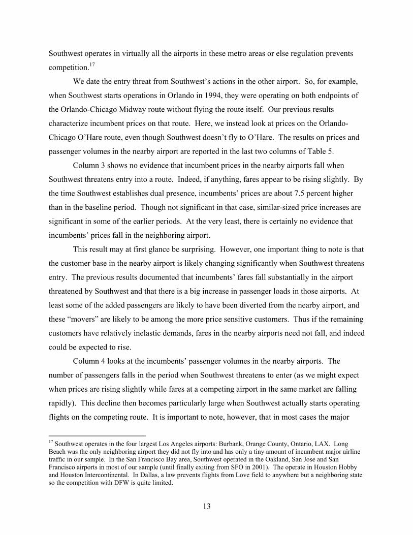
Southwest operates in virtually all the airports in these metro areas or else regulation prevents
competition.17
We date the entry threat from Southwest’s actions in the other airport. So, for example,
when Southwest starts operations in Orlando in 1994, they were operating on both endpoints of
the Orlando-Chicago Midway route without flying the route itself. Our previous results
characterize incumbent prices on that route. Here, we instead look at prices on the Orlando-
Chicago O’Hare route, even though Southwest doesn’t fly to O’Hare. The results on prices and
passenger volumes in the nearby airport are reported in the last two columns of Table 5.
Column 3 shows no evidence that incumbent prices in the nearby airports fall when
Southwest threatens entry into a route. Indeed, if anything, fares appear to be rising slightly. By
the time Southwest establishes dual presence, incumbents’ prices are about 7.5 percent higher
than in the baseline period. Though not significant in that case, similar-sized price increases are
significant in some of the earlier periods. At the very least, there is certainly no evidence that
incumbents’ prices fall in the neighboring airport.
This result may at first glance be surprising. However, one important thing to note is that
the customer base in the nearby airport is likely changing significantly when Southwest threatens
entry. The previous results documented that incumbents’ fares fall substantially in the airport
threatened by Southwest and that there is a big increase in passenger loads in those airports. At
least some of the added passengers are likely to have been diverted from the nearby airport, and
these “movers” are likely to be among the more price sensitive customers. Thus if the remaining
customers have relatively inelastic demands, fares in the nearby airports need not fall, and indeed
could be expected to rise.
Column 4 looks at the incumbents’ passenger volumes in the nearby airports. The
number of passengers falls in the period when Southwest threatens to enter (as we might expect
when prices are rising slightly while fares at a competing airport in the same market are falling
rapidly). This decline then becomes particularly large when Southwest actually starts operating
flights on the competing route. It is important to note, however, that in most cases the major
17 Southwest operates in the four largest Los Angeles airports: Burbank, Orange County, Ontario, LAX. Long Beach was the only neighboring airport they did not fly into and has only a tiny amount of incumbent major airline traffic in our sample. In the San Francisco Bay area, Southwest operated in the Oakland, San Jose and San Francisco airports in most of our sample (until finally exiting from SFO in 2001). The operate in Houston Hobby and Houston Intercontinental. In Dallas, a law prevents flights from Love field to anywhere but a neighboring state so the competition with DFW is quite limited.
13

incumbents at the Southwest airport and at the nearby airport are not the same. In Chicago, for
example, Continental is an incumbent that mainly flies out of Chicago-Midway while United
flies exclusively out of O’Hare. The estimated effects do not imply that the same carrier is
diverting passengers from its flights at one airport to its flights at another.
VI. How and Why Do Incumbents Respond Early?
The results above document significant fare changes by incumbents in response to a
threat of entry even before there is any outright competition from Southwest. Less clear is what
the incumbents are trying to accomplish by doing so.
A. Capacity and Load Factor
The first thing we consider is whether the airlines are primarily cutting prices while
holding their fleet size fixed (pursuing the intensive margin) or whether prices are falling as the
by-product of capacity expansion, perhaps as some form of strategic investment to deter entry.
Unfortunately, the DB1A files used to construct our core sample are a sample of tickets, not
flights, so they cannot speak to capacity issues like the number of flights on a route. We can get
that type of information, however, from the T-100 data of the U.S. Department of
Transportation. These data, rather than being a ticket-based sample, contain aggregate
information at the segment-carrier-month level which we aggregate up to the route-carrier-
quarter level to match our DB1A-based data. The data include the total number of passengers,
the number of flights, and the total available seats on each segment. This data source also
provides an independent check on the passenger number results obtained above using the DB1A
data.
There are two problems with using the T-100 for our purposes. The first and more minor
one results from the T-100 being based on segments rather than flights as in the DB1A. It does
not count as a segment a direct flight that makes a stop without changing planes, though that
would count as direct in the DB1A.18 Second, and more importantly, the T-100 has serious
coverage problems when the number of passengers on a segment is small. When we compare
the T-100 to our sample of 18,969 direct flight route-carrier-quarters in the DB1A, there are only
18 A flight from Chicago O’Hare (ORD) to Washington Dulles (IAD), for example, that stops but does not involve a change of plane would show up as a direct flight in the DB1A but not as an ORD-IAD segment in the T-100.
14

3,464 matches in the T-100. The main source of the problem is that whereas the DB1A has each
route in the sample for an average of 18 quarters, the T-100 has roughly half that. In the T-100,
flights appear to start, stop, and start again. Correspondingly, the match quality is much worse
for the smallest segments. This matching problem is clearly concentrated in the smaller routes,
however. The T-100 accounts for only about 20 percent of the route-carrier-quarters in the
DB1A sample, but those 20 percent account for 95 percent of the total passengers in the DB1A.
Since we our weighting each route in our regressions by the number of passengers, we are less
concerned about the missing routes.
To see this in the case of passenger loads, in column 1 of Table 6 we restrict the larger
DB1A sample to only those route-carrier-quarters that are also in the T-100. The results for
passengers are similar to the full-sample DB1A results. Next, in column 2, we report the
corresponding estimates using the T-100’s independent measure of total passengers flown by the
incumbents. These show results comparable to those from the DB1A. There is a significant
increase in the number of passengers surrounding the threat of Southwest entry, with the
magnitude and the timing showing marked similarities across the two data sets. Indeed the total
effect on passengers is slightly larger in the T-100 than in the core sample.
We look at two measures of incumbent capacity on threatened routes in columns 3 and 4.
Column 3 shows results for the logged number of seats available and column 4 for the logged
number of flights. In both cases, there are positive but insignificant coefficients; while we
cannot rule out a rise in capacity, the evidence for it is not strong. In column 5, we look at the
log of the load factor (the share of available seats on the flights that had passengers in them).
Here, we find statistically significant evidence that, regardless of whether the number of flights
grows, significantly more people are flying per plane. The point estimates imply that at least 50
to 60 percent of the increase in traffic comes from higher number of passengers per plane rather
than just expanding the number of planes.
B. Frequent Flyers
As discussed above, frequent flyer programs are a mechanism that would provide a
motive for the observed incumbent fare cuts upon Southwest’s entry threat (but before its actual
entry into the route). If incumbents can induce people to fly more in the period just before
Southwest’s entry, and passengers with a greater stock of miles on a particular carrier are less
15

likely to try a new airline, this could serve as a type of long-term-contract-type barrier to entry.
This also implies that incumbents get the “biggest bang for their buck” by directing the greatest
price drops to their passengers enrolled in frequent flyer programs.
Unfortunately we do not directly observe the preponderance of frequent flyer program
members in specific cities or on specific routes, so our evidence will be indirect and probably
best characterized as suggestive. We know that business travelers are the biggest users of loyalty
programs (and the customers most sought after by the incumbents with those programs).19
Business travelers tend to be the higher fare customers, so if their loyalty is the driving factor for
the incumbents’ pre-emptive responses, the price cuts should be concentrated among very
different groups and locations than if they are simply trying to meet competition for low-end
leisure travelers.
Although the DB1A data has no direct information about business travelers, we can look
at fare quantiles to see what is happening at various points in the fare distribution. Since
business travelers disproportionately account for high-fare tickets, we should therefore expect to
see fares on threatened routes fall more at the high end of the distribution.20 We present results
of estimating (1) using the 25th, 50th and 75th percentile logged fares in columns 1 through 3,
respectively, of Table 7 (here we return to the DB1A sample). The fares at each of these three
quantiles fall significantly from the threat of entry, but the point estimates indicate that the 50th-
and 75th-percentile fares fall by about 50 percent more than the 25th-percentile fares. The
standard errors are too large to reject equality, though, so this result is somewhat tentative.21
As a second, more direct test, we compare fares on threatened routes that are more
heavily populated with leisure travelers to those without. We classify routes by leisure status
similarly to Borenstein (1989): for each endpoint airport’s corresponding state, we compute the
fraction of 1998 gross state product accounted for by the hotel industry. If this fraction is above
1 percent for either endpoint of a route, we classify it a leisure-intensive route. The others we 19 See, for example, Alden (2004). 20 A separate mechanism that would also present a demand-building motive for incumbents with regard to their business travelers is that substantial business travel takes place using tickets purchased as a result of direct negotiation between large employers and incumbent carriers. A threatened incumbent may be willing to negotiate more generous deals (which would show up in our data as a drop in average fares) in order to hold such corporate business. 21 Another caveat is that we cannot rule out the possibility that these results arise because markups are greater at the higher end of the distribution, and that, as with the results by route concentration above, threatened entry has a greater impact on high-markup fares.
16

classify as business-intensive. Columns 4 and 5 present the results on fare changes for routes
that are leisure- and business-intensive are shown in columns 4 and 5 of the table. Fares fall
more on business routes when Southwest threatens entry. While the declines are significant in
both columns, they are roughly twice as large on the business routes.
The results presented in this section are consistent with the notion that the fare drops on
threatened routes reflect efforts by the incumbent to build up switching costs among its frequent-
flying business customers prior to Southwest’s entry, either to deter entry altogether or to put the
incumbent in a better ex-post competitive position should entry occur.
VII. Discussion and Conclusion
This paper has looked at the response of incumbent major airlines to the threat of entry by
examining how the incumbents respond when Southwest starts operating in the airports on both
ends of a route but before it actually starts flying that route. The nature of Southwest’s network
means that the likelihood of their entering such a route rises dramatically when Southwest starts
operating in the second endpoint airport, thus generating a discrete change in incumbents’
expectations about the likelihood of new competition through entry.
The results indicate that incumbents do indeed react to the threat of Southwest’s entry
before actual entry takes place. Incumbents drop fares significantly in anticipation of entry.
This is not simply due to airport-specific cost shocks because fares drop on threatened routes
relative to incumbents’ fares on other routes from the same airports. The fare declines are
accompanied by a sizable increase in the number of passengers flying the incumbents’ threatened
routes. The fare decreases are largest for routes that are concentrated beforehand, but do not
decrease at all for routes into neighboring airports in the same MSA (i.e., where Southwest is not
directly threatening entry). There is only weak evidence that the incumbents expand capacity
(the number of available seats and flights), but there is strong evidence that load factors increase
on those flights they have.
In the end, the results are consistent with a view that the incumbents are attempting to
establish some kind of long-term loyalty on the part of their customers before those customers
have a new carrier to choose from. One natural source of such loyalty are frequent flyer
programs, though there are potentially other more amorphous mechanisms like brand loyalty.
Consistent with the frequent flyer story, quantile regressions suggest that the incumbent
17

responses to the threat of entry are greatest among the higher fares (where frequent flyers are
more prevalent) and on more business-traveler-intensive routes.
The findings of this paper suggest that Southwest Airlines has a powerful competitive
effect in the U.S. passenger airline industry, and that this effect does not operate solely through
Southwest’s head-to-head competition with major carriers. Substantial fare reductions from
major carriers are induced merely by the threat of competing with Southwest. We have focused
on the U.S. passenger airline industry in particular because it offers a good setting to empirically
identify the causes and effects of interest, and to therefore add to the still sparse empirical
literature on the threat of entry. If the response of incumbents here is anything like the responses
in other industries, the study of preemption and customer loyalty may be fruitful avenues for
future empirical research.
18

References Aghion, Philippe and Patrick Bolton. “Contracts as a Barrier to Entry.” American Economic
Review, 77(3), 1987, 388-401. Alden, Sharyn. “FAQs About Frequent Flyer Miles.” Money Savvy, Credit Union National
Association, Inc., 2004. Bailey, Elizabeth E. “Contestability and the Design of Regulatory and Antitrust Policy.”
American Economic Review, 71(2), 1981, 178-183. Bamberger, Gustavo E., Dennis W. Carlton, and Lynette R. Neumann. “An Empirical
Investigation of the Competitive Effects of Domestic Airline Alliances.” NBER Working Paper No. 8197, 2001.
Berry, Steven T. “Estimation of a Model of Entry in the Airline Industry.” Econometrica, 60(4),
1992, 889-917. Borenstein, Severin. “Hubs and High Fares: Dominance and Market Power in the U.S. Airline
Industry.” RAND Journal of Economics, 20(3), 1989, 344-365. Borenstein, Severin. “The Dominant-Firm Advantage in Multiproduct Industries: Evidence from
the U. S. Airlines.” Quarterly Journal of Economics, 106(4), 1991, 1237-1266. Borenstein, Severin. “The Evolution of U.S. Airline Competition.” Journal of Economic
Perspectives, 6(2), 1992, 45-73. Borenstein, Severin. “Repeat-Buyer Programs in Network Industries.” in Werner Sichel ed.,
Networks, Infrastructure, and The New Task for Regulation, University of Michigan Press, 1996.
Borenstein, Severin and Nancy L. Rose. “Competition and Price Dispersion in the U.S. Airline
Industry.” The Journal of Political Economy, 102(4), 1994, 653-683. Brueckner, Jan, Nichola Dyer and Pablo T. Spiller. “Fare Determination in Airline Hub and
Spoke Networks,” RAND Journal of Economics, 23, 1992, 309-333. Cairns, Robert D. and John W. Galbraith. “Artificial Compatibility, Barriers to Entry and
Frequent Flyer Programs,” Canadian Journal of Economics, 23(4), 1990, 807-816. Dixit, Avinash. “A Model of Duopoly Suggesting a Theory of Entry Barriers.” Bell Journal of
Economics, 10(1), 1979, 20-32. Ellison, Glenn and Sara Fisher Ellison (2000), "Strategic Entry Deterrence and the Behavior of
Pharmaceutical Incumbents Prior to Patent Exploration," MIT Working Paper

Evans, William N. and Ioannis Kessides. “Localized Market Power in the U.S. Airline Industry.” Review of Economics and Statistics, 75(1), 1993, 66-75.
Gillen, David, William Morrison, and Christopher Stewart, "Air Travel Demand Elasticities:
Concepts, Issues, and Measurement," Department of Finance, Canada, January 23, 2003, available at <http://www.fin.gc.ca/consultresp/Airtravel/airtravStdy_e.html>
Hendricks, Ken, Michelle Piccione, and Guofu Tan. “Entry and Exit in Hub-Spoke Networks.”
Rand Journal of Economics, 28(2), 1997, 291-303. Hurdle, Gloria J., Richard L. Johnson, Andrew S. Joskow, Gregory J. Werden, Michael A.
Williams. “Concentration, Potential Entry, and Performance in the Airline Industry.” Journal of Industrial Economics, 38(2), 1989, 119-139.
Klemperer, Paul. “Entry Deterrence in Markets with Consumer Switching Costs.” The Economic
Journal, 97(Supplement: Conference Papers), 1987, 99-117. Lederman, Mara. “Do Enhancements to Loyalty Programs Affect Demand? The Impact of
International Frequent Flyer Partnerships on Domestic Airline Demand.” Working Paper, Rotman School of Management, University of Toronto, 2004.
Mayer, Chris and Todd Sinai. “Network Effects, Congestion Externalities, and Air Traffic
Delays: Or Why All Delays Are Not Evil.” American Economic Review, 93(4), 2003, 1194-1215.
Milgrom, Paul and John Roberts. “Limit Pricing and Entry Under Incomplete Information: An
Equilibrium Analysis.” Econometrica, 50(2), 1982, 443-460. Morrison, Steven A. “Actual, Adjacent, and Potential Competition: Estimating the Full Effect of
Southwest Airlines.” Journal of Transport Economics and Policy, 32(2), 2001, 239-256. Morrison, Steven A., and Clifford Winston. “Enhancing the Performance of the Deregulated Air
Transportation System.” Brookings Papers on Economic Activity, Microeconomics, 1, 1989, 61-112.
Reiss, Peter C. and Pablo T. Spiller. “Competition and Entry in Small Airline Markets.” Journal
of Law and Economics, 32, 1989, S179-S202. Selten, Reinhard. “The Chain Store Paradox.” Theory and Decision, 9(2), 1978, pp. 127-159. Spence, Michael. “The Learning Curve and Competition.” Bell Journal of Economics, 12(1),
1981, 49-70. Whinston, Michael D. and Scott C. Collins. “Entry and Competitive Structure in Deregulated
Airline Markets: An Event Study Analysis of People Express.” RAND Journal of Economics, 23(4), 1992, 445-462.

Figure 1. Identifying a Threatened Incumbent Route
Philadelphia, PA Southwest presence 2004: Q2
Southwest threatens entry here when they start operations in both endpoint airports
Jacksonville, FL Southwest presence 1997: Q1
Tampa, FL Southwest presence 1996: Q1

Figure 2. Comparison Routes for PHL-JAX
Philadelphia, PA
Non-Southwest Airports
Airport 1 alternate routes
Airport 2 alternate routes
Jacksonville, FL

Table 1. Probability of Southwest’s Entry into a Route
Southwest operates in one endpoint airport in the previous quarter (single presence)
0.003 (0.000)
Southwest operates in both endpoint airports in the previous quarter (dual presence)
0.169 (0.020)
N 143,380 Notes: The table shows estimates from a probit estimation for Southwest’s entry into a route in a particular quarter, conditional on the number of the route’s endpoint airports served by Southwest in the previous quarter. The excluded category includes observations where Southwest does not serve either endpoint airport in the previous quarter. Quarter fixed effects are included. Standard errors are in parentheses.
Table 2. Descriptive Statistics, Fare and Passenger Summaries
Mean (std deviation) Direct Flights to Threatened Airport
Avg. ln(fare) ln(passengers)
Number of Threatened Routes
Route-Carrier-Quarters in sample
Direct Flights to Neighboring Airport Avg. ln(fare)
ln(passengers)
Number of Threatened Routes Route-Carrier-Quarters in sample
5.21 (0.45) 2.55 (2.13)
678
18,969
5.16 (0.48) 3.81 (2.69)
169
7,296 Notes: Authors' calculations using the DB1A database from the U.S. Department of Transportation.

Table 3. Basic Results
(1) (2) (3) (4) Dependent Variable: ln(p) ln(p) ln(q) ln(q)
Entry defined by: direct flight any flight direct
flight any flight
Southwest in both airports (no flights) t0-8 to t0-7
-.047 (.019)
-.037 (.050)
.017 (.037)
.042 (.055)
Southwest in both airports (no flights) t0-6 to t0-5
-.044 (.033)
-.010 (.039)
.000 (.051)
.006 (.059)
Southwest in both airports (no flights) t0-4 to t0-3
-.107 (.037)
-.073 (.042)
.129 (.055)
.129 (.058)
Southwest in both airports (no flights) t0-2 to t0-1
-.151 (.044)
-.097 (.050)
.125 (.085)
.061 (.075)
Southwest in both airports (no flights) t0
-.187 (.051)
-.153 (.062)
.132 (.087)
.095 (.083)
Southwest in both airports (no flights) t0+1 to t0+2
-.189 (.051)
-.221 (.066)
.095 (.086)
.102 (.087)
Southwest in both airports (no flights) t0+3 to t0+12
-.260 (.055)
-.300 (.075)
.151 (.084)
.192 (.091)
Southwest flying route te
-.256 (.055)
-.185 (.071)
.118 (.100)
.066 (.087)
Southwest flying route te+1 to te+2
-.271 (.073)
-.226 (.070)
.115 (.100)
.067 (.099)
Southwest flying route te+3 to te+12
-.321 (.082)
-.234 (.076)
.142 (.115)
.118 (.106)
N 18,969 15,819 18,969 15,819 R2 .89 .84 .94 .93
Notes: This table shows estimates from passenger-weighted average logged fares and logged total passengers for our baseline sample. All regressions include route-carrier and quarter fixed effects. Standard errors are in parentheses and are clustered by route to account for correlation across time and across carriers on the same route. The sample includes all routes where Southwest threatens entry as defined in the text. The “Southwest in both airports” dummies denote Southwest having flights involving airports on both ends of a route previous to actually flying the route. The “Southwest flying route” dummies denote Southwest actually operating flights on the route. Columns (1) and (3) define Southwest airlines as entering a route when they establish direct service between the two airports. Columns (2) and (4) define entry as establishing either direct or change-of-plane service, where the latter is defined as having in the sample at least 40 change-of-plane Southwest tickets for the route.
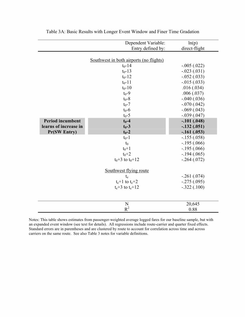
Table 3A: Basic Results with Longer Event Window and Finer Time Gradation
Dependent Variable: ln(p) Entry defined by: direct-flight
Period incumbent learns of increase in
Pr(SW Entry)
Southwest in both airports (no flights)
t0-14 t0-13 t0-12 t0-11 t0-10 t0-9 t0-8 t0-7 t0-6 t0-5 t0-4 t0-3 t0-2 t0-1 t0
t0+1 t0+2
t0+3 to t0+12
Southwest flying route te
te+1 to te+2 te+3 to te+12
-.005 (.022) -.023 (.031) -.052 (.033) -.015 (.033) .016 (.034) .006 (.037) -.040 (.036) -.070 (.042) -.069 (.043) -.039 (.047) -.101 (.048) -.132 (.051) -.161 (.053) -.155 (.058) -.195 (.066) -.195 (.066) -.194 (.065) -.264 (.072)
-.261 (.074) -.275 (.095) -.322 (.100)
N R2
20,645 0.88
Notes: This table shows estimates from passenger-weighted average logged fares for our baseline sample, but with an expanded event window (see text for details). All regressions include route-carrier and quarter fixed effects. Standard errors are in parentheses and are clustered by route to account for correlation across time and across carriers on the same route. See also Table 3 notes for variable definitions.

Table 4. Incumbent Average Fare Responses, Adjusted for Operating Cost Proxies
(1) Baseline
(2) Alternates 1
(3) Alternates 2
(4) cost controls
Southwest in both airports (no flights) t0-8 to t0-7
-.047 (.019)
-.050 (.040)
-.036 (.029)
-.030 (.018)
Southwest in both airports (no flights) t0-6 to t0-5
-.044 (.033)
-.076 (.058)
-.026 (.041)
-.034 (.030)
Southwest in both airports (no flights) t0-4 to t0-3
-.107 (.037)
-.144 (.065)
-.093 (.048)
-.086 (.035)
Southwest in both airports (no flights) t0-2 to t0-1
-.151 (.044)
-.208 (.079)
-.164 (.052)
-.143 (.041)
Southwest in both airports (no flights) t0
-.187 (.051)
-.237 (.083)
-.201 (.057)
-.176 (.049)
Southwest in both airports (no flights) t0+1 to t0+2
-.189 (.051)
-.235 (.085)
-.219 (.053)
-.162 (.043)
Southwest in both airports (no flights) t0+3 to t0+12
-.260 (.055)
-.257 (.095)
-.278 (.061)
-.222 (.047)
Southwest flying route te
-.256 (.055)
-.320 (.113)
-.290 (.072)
-.236 (.056)
Southwest flying route te+1 to te+2
-.271 (.073)
-.314 (.106)
-.333 (.081)
-.259 (.056)
Southwest flying route te+3 to te+12
-.321 (.082)
-.384 (.124)
-.378 (.095)
-.312 (.063)
Operating cost control, endpoint airport 1 - - .404
(.059) Operating cost control,
endpoint airport 2 - - .297 (.064)
N 18,969 17,239 18,498 18,146 R2 .89 .84 .87 .91
Notes: All regressions are weighted by passengers and include route-carrier and quarter fixed effects. Standard errors are in parentheses and are clustered by route to account for correlation across time and across carriers on the same route. The dependent variable in columns (1) and (4) is the average log of fares for the route-carrier. The dependent variable in column (2) is the average log price of direct flights minus the price of direct flights by the same carrier between endpoint airport 1 and alternative airports that Southwest does not fly to. The dependent variable in column (3) is the price of direct flights on the route minus the price of direct flights by the same carrier between endpoint airport 2 and alternative airports that Southwest does not fly to. The operating cost controls are defined as average fares for the same carrier between the stated airport and cities that Southwest Airlines does not fly. See also Table 3 notes for variable definitions.

Table 5. Results by Type of Route
(1)
ln(p) low HHI routes
(2) ln(p)
high HHI routes
(3) ln(p)
nearby airport
(4) ln(q)
nearby airportSW in both airports (no flights)
t0-8 to t0-7 -.012 (.036)
-.054 (.024)
.017 (.043)
-.006 (.050)
SW in both airports (no flights) t0-6 to t0-5
.048 (.057)
-.056 (.026)
.123 (.054)
-.164 (.066)
SW in both airports (no flights) t0-4 to t0-3
.035 (.068)
-.122 (.027)
.101 (.057)
-.086 (.076)
SW in both airports (no flights) t0-2 to t0-1
.031 (.075)
-.167 (.036)
.132 (.064)
-.200 (.082)
SW in both airports (no flights) t0
-.017 (.082)
-.202 (.045)
.076 (.051)
-.186 (.097)
SW in both airports (no flights) t0+1 to t0+2
-.051 (.085)
-.196 (.036)
.132 (.052)
-.225 (.105)
SW in both airports (no flights) t0+3 to t0+12
-.168 (.123)
-.266 (.044)
.170 (.076)
-.322 (.128)
SW flying route te
-.078 (.117)
-.270 (.059)
.176 (.071)
-.340 (.137)
SW flying route te+1 to te+2
-.122 (.107)
-.282 (.049)
.159 (.069)
-.302 (.133)
SW flying route te+3 to te+12
-.151 (.125)
-.333 (.052)
.170 (.077)
-.342 (.151)
N 9498 9200 7296 7296 R2 .86 .89 .88 .89
Notes: All regressions are weighted by passengers and include route-carrier and quarter fixed effects. Standard errors are in parentheses and are clustered by route to account for correlation across time and across carriers on the same route. The dependent variable in columns (1), (2) and (3) is the average log of fares for the route-carrier. The dependent variable in (4) is the log number of passengers. Columns (1) and (2) divide the sample between routes that have HHI concentrations at or below the median in the sample and routes with HHI concentrations above the median. Columns (3) and (4) look at the price and quantity responses on routes to neighboring airports that Southwest does not fly to but are in the same market as an airport where Southwest does operate. See also Table 3 notes for variable definitions.

Table 6. Incumbent Capacity Responses: Flights, Seats, and Load Factors
Dependent Variable:
Data Source:
(1) ln(q)
DB1A
(2) ln(q) T100
(3) ln(seats)
T100
(4) ln(flights)
T100
(5) ln(load factor)
T100 SW in both airports (no flights)
t0-8 to t0-7 .014
(.040) .007
(.048) .009
(.040) .001
(.038) -.001 (.024)
SW in both airports (no flights) t0-6 to t0-5
.026 (.054)
-.030 (.070)
-.026 (.067)
-.034 (.060)
-.002 (.029)
SW in both airports (no flights) t0-4 to t0-3
.171 (.058)
.132 (.056)
.058 (.059)
.051 (.055)
.073 (.030)
SW in both airports (no flights) t0-2 to t0-1
.170 (.090)
.143 (.084)
.069 (.092)
.056 (.079)
.071 (.037)
SW in both airports (no flights) t0
.181 (.092)
.242 (.094)
.123 (.100)
.106 (.088)
.121 (.046)
SW in both airports (no flights) t0+1 to t0+2
.145 (.091)
.195 (.099)
.092 (.103)
.074 (.092)
.103 (.049)
SW in both airports (no flights) t0+3 to t0+12
.205 (.088)
.217 (.093)
.082 (.104)
.060 (.095)
.135 (.053)
SW flying route te
.180 (.105)
.289 (.117)
.158 (.121)
.115 (.110)
.132 (.071)
SW flying route te+1 to te+2
.181 (.103)
.286 (.118
.189 (.125)
.144 (.108)
.097 (.063)
SW flying route te+3 to te+12
.208 (.122)
.322 (.130)
.204 (.134)
.155 (.124)
.118 (.071)
N 3464 3464 3489 3489 3464 R2 .93 .92 .93 .92 .71
Notes: All regressions are weighted by passengers and include route-carrier and quarter fixed effects. Standard errors are in parentheses and are clustered by route to account for correlation across time and across carriers on the same route. The dependent variable in columns (1) and (2) is the log number of passengers. The dependent variable in (3) is the log of the total number of seats available on the route. In (4) it is the log number of flights actually flown. In (5) it is the share of the seats flown that are filled with passengers. The data set for column (1) is the DB1A whereas the data set for columns (2)-(5) is the T-100 as explained in the text. The sample in (1) is restricted to the same routes as in the T-100. See also Table 3 notes for variable definitions.

Table 7. Frequent Flyers and the Fare Declines
(1) ln(p)
25th pctile
(2) ln(p)
50th pctile
(3) ln(p)
75th pctile
(4) ln(p)
leisure routes
(5) ln(p)
business routes
SW in both airports (no flights) t0-8 to t0-7
-.043 (.021)
-.066 (.025)
-.048 (.032)
-.024 (.022)
-.085 (.044)
SW in both airports (no flights) t0-6 to t0-5
-.059 (.026)
-.079 (.038)
-.011 (.045)
-.034 (.021)
-.047 (.050)
SW in both airports (no flights) t0-4 to t0-3
-.100 (.028)
-.168 (.045)
-.151 (.060)
-.061 (.025)
-.147 (.053)
SW in both airports (no flights) t0-2 to t0-1
-.127 (.034)
-.189 (.057)
-.205 (.070)
-.092 (.036)
-.197 (.061)
SW in both airports (no flights) t0
-.157 (.039)
-.227 (.064)
-.241 (.084)
-.139 (.053)
-.235 (.072)
SW in both airports (no flights) t0+1 to t0+2
-.173 (.044)
-.233 (.067)
-.237 (.082)
-.142 (.039)
-.240 (.069)
SW in both airports (no flights) t0+3 to t0+12
-.220 (.053)
-.280 (.075)
-.333 (.097)
-.187 (.051)
-.335 (.077)
SW flying route te
-.177 (.056)
-.263 (.074)
-.311 (.091)
-.158 (.060)
-.337 (.102)
SW flying route te+1 to te+2
-.207 (.084)
-.299 (.100)
-.310 (.110)
-.130 (.044)
-.400 (.090)
SW flying route te+3 to te+12
-.300 (.075)
-.353 (.101)
-.323 (.127)
-.153 (.049)
-.484 (.097)
N 18,968 18,968 18,968 8849 10120 R2 .81 .79 .82 .85 .91
Notes: All regressions are weighted by passengers and include route-carrier and quarter fixed effects. Standard errors are in parentheses and are clustered by route to account for correlation across time and across carriers on the same route. Columns (1)-(3) present quantile regressions for the 25th, 50th and 75th percentiles or prices on a route. The dependent variable in columns (4)-(5) is the average log of fares for the route-carrier. Columns (4) and (5) divide the sample according to whether or not the routes have at least one endpoint in a “leisure” destination state. See text for details. See also Table 3 notes for variable definitions.