How Can We Outlive Our Way of Life? - OECD...How Can We Outlive Our Way of Life? Tad W. Patzek Department of Civil and Environmental Engineering The University of California Berkeley,

How Can We Outlive

Our Way of Life?

Tad W. PatzekDepartment of Civil and Environmental Engineering

The University of CaliforniaBerkeley, CA 94720

[email protected]

Paper prepared for the 20th Round Table on SustainableDevelopment of Biofuels: Is the Cure Worse than the Disease?

OECD Headquarters, Chateau de la Muette, Paris, 11-12 September 2007

September 10, 2007

Abstract

In this paper I outline the rational, science-based arguments that question current wis-dom of replacing fossil plant fuels (coal, oil and natural gas) with fresh plant agrofuels. This1:1 replacement is absolutely impossible for more than a few years, because of the ways theplanet Earth works and maintains life. After these few years, the denuded Earth will be adifferent planet, hostile to human life. I argue that with the current set of objective con-straints a continuous stable solution to human life cannot exist in the near-future, unless weall rapidly implement much more limited ways of using the Earth’s resources, while reduc-ing the global populations of cars, trucks, livestock and, eventually, also humans. To avoideconomic and ecological disasters, I recommend to decrease all automotive fuel use in Eu-rope by up to 6 percent per year in 8 years, while switching to the increasingly rechargeablehybrid and all-electric cars, progressively driven by photovoltaic cells. The actual scheduleof the rate of decrease should also depend on the exigencies of greenhouse gas abatement.The photovoltaic cell-battery-electric motor system is some 100 times more efficient thanmajor agrofuel systems.

Contents

1 Recommendations 4

2 Glossary 5

3 Introduction 6

4 Background 9

4.1 Problems with Change . . . . . . . . . . . . . . . . . . . . . . . . . . . . . . . . . 11

4.2 But Plant Biology is Different! . . . . . . . . . . . . . . . . . . . . . . . . . . . . 12

5 Plan of Attack 14

1

6 Efficiency of Cellulosic Ethanol Refineries 156.1 Iogen Ottawa Facility . . . . . . . . . . . . . . . . . . . . . . . . . . . . . . . . . 156.2 Proposed Cellulosic Ethanol Refineries . . . . . . . . . . . . . . . . . . . . . . . . 17

7 Where Will the Agrofuel Biomass Come From? 197.1 Useful Terminology . . . . . . . . . . . . . . . . . . . . . . . . . . . . . . . . . . . 197.2 Plant Biomass Production . . . . . . . . . . . . . . . . . . . . . . . . . . . . . . . 207.3 Is There Any Other Proof of NEP = 0? . . . . . . . . . . . . . . . . . . . . . . . 227.4 Satellite Sensor-based Estimates . . . . . . . . . . . . . . . . . . . . . . . . . . . 237.5 NPP in the US . . . . . . . . . . . . . . . . . . . . . . . . . . . . . . . . . . . . . 25

8 Photovoltaic Cells vs. Agrofuels 288.1 General Comparisons . . . . . . . . . . . . . . . . . . . . . . . . . . . . . . . . . . 288.2 US corn-ethanol system . . . . . . . . . . . . . . . . . . . . . . . . . . . . . . . . 288.3 Acacia-for-energy system . . . . . . . . . . . . . . . . . . . . . . . . . . . . . . . . 288.4 Eucalyptus-for-energy system . . . . . . . . . . . . . . . . . . . . . . . . . . . . . 308.5 Sugarcane-for-energy system . . . . . . . . . . . . . . . . . . . . . . . . . . . . . . 318.6 Driving on Solar Power . . . . . . . . . . . . . . . . . . . . . . . . . . . . . . . . 35

8.6.1 Calculation Results . . . . . . . . . . . . . . . . . . . . . . . . . . . . . . . 35

9 Conclusions 38

A Ecosystem Definition and Properties 42

B Mass Balance of Carbon in an Ecosystem 44

C Environmental Controls on Net Primary Productivity 48

List of Tables

1 Yields of ethanol from cellulose and hemicellulose . . . . . . . . . . . . . . . . . . 162 GPP/NPP global sums . . . . . . . . . . . . . . . . . . . . . . . . . . . . . . . . 233 2003 US NPP by ground cover class . . . . . . . . . . . . . . . . . . . . . . . . . 264 2003 US NPP by lumped ground cover classs . . . . . . . . . . . . . . . . . . . . 265 Free energy balance of US corn-ethanol system . . . . . . . . . . . . . . . . . . . 296 Free energy balances of acacia and eucalypt plantation-energy systems . . . . . . 307 Free energy balance of sugarcane-ethanol system . . . . . . . . . . . . . . . . . . 328 Areas to power a car from different energy sources . . . . . . . . . . . . . . . . . 369 Summary of global carbon fluxes . . . . . . . . . . . . . . . . . . . . . . . . . . . 4710 Average NPP . . . . . . . . . . . . . . . . . . . . . . . . . . . . . . . . . . . . . . 49

List of Figures

1 Liquid transportation fuel use in the US . . . . . . . . . . . . . . . . . . . . . . . 72 35 billion gallons of ethanol in 10 years . . . . . . . . . . . . . . . . . . . . . . . . 73 Exponential growth of world crude oil production . . . . . . . . . . . . . . . . . . 84 US petroleum consumption and global production of conventional petroleum . . 85 An Earth system . . . . . . . . . . . . . . . . . . . . . . . . . . . . . . . . . . . . 96 Global population . . . . . . . . . . . . . . . . . . . . . . . . . . . . . . . . . . . 107 World crude oil production . . . . . . . . . . . . . . . . . . . . . . . . . . . . . . 108 Human-appropriated Net Primary Production . . . . . . . . . . . . . . . . . . . . 119 Ecological cycles . . . . . . . . . . . . . . . . . . . . . . . . . . . . . . . . . . . . 1210 A linear process in industry . . . . . . . . . . . . . . . . . . . . . . . . . . . . . . 13

2

11 Havoc from Indonesia’s oil palm plantation fires . . . . . . . . . . . . . . . . . . . 1412 Ethanol production in Iogen’s Ottawa plant . . . . . . . . . . . . . . . . . . . . . 1513 Steam requirement in ethanol beer distillation . . . . . . . . . . . . . . . . . . . . 1714 Stated energy efficiencies of future cellulosic ethanol refineries . . . . . . . . . . . 1815 Global organic carbon burial during the Phanerozoic eon. . . . . . . . . . . . . . 2016 Net ecosystem productivity of a forest . . . . . . . . . . . . . . . . . . . . . . . . 2117 NPP’s of Asia-Pacific, South America, and Europe – relative to North America . 2218 Burning tropical forest in Central Africa . . . . . . . . . . . . . . . . . . . . . . . 2419 MOD17A2/A3-based calculation of US NPP in 2003 . . . . . . . . . . . . . . . . . 2520 US primary energy consumption and NPP in 2003 . . . . . . . . . . . . . . . . . 2721 Captured solar energy . . . . . . . . . . . . . . . . . . . . . . . . . . . . . . . . . 2922 Primary power delivered by renewable systems . . . . . . . . . . . . . . . . . . . 3023 Free energy flows in US corn-ethanol system . . . . . . . . . . . . . . . . . . . . . 3124 Free energy flows in a tropical A. mangium plantation-agrofuel system . . . . . . 3225 Free energy flows in by a tropical E. deglupta plantation-agrofuel system . . . . . 3326 Free energy flows in a tropical sugarcane plantation-ethanol refinery in Brazil . . 3427 Fractional area to restore free-energy costs of power generation . . . . . . . . . . 3628 Net land areas needed to power a car from different sources . . . . . . . . . . . . 3729 Total land areas needed to power a car from different sources . . . . . . . . . . . 3730 Photosynthesis schematic . . . . . . . . . . . . . . . . . . . . . . . . . . . . . . . 4331 Crop yield vs. soil loss . . . . . . . . . . . . . . . . . . . . . . . . . . . . . . . . . 47

3

1 Recommendations

As I show in this paper, the solar power captured by industrial corn, tree, and sugarcaneplantations is minuscule when compared with our current use of oil (which will last for a limitedtime only) or the potential provided by photovoltaic solar cells (which will last practicallyforever). To make things worse, what little solar energy is captured by the plants goes intandem with a disproportionate environmental damage and negative free energy balance ofagrosystems. Therefore, choosing between solar cells and agrofuels, government and industrialfunding for renewable energy sources would be spent ∼100 times more wisely on the developmentof large-throughput, efficient technologies of manufacturing solar cells and batteries.

My recommendations are as follows:

1. As I show here, significantly more efficient individual transportation systems are possibleand ought to be implemented. Wherever sensible, individual transportation should bereplaced with public transportation systems.

2. The average rate of decline of conventional petroleum production in the world will gradu-ally increase to about 6% per year, and only some of this production will be temporarilyreplaced by unconventional petroleum sources (tar sands, ultra-heavy oil, oil shale, etc.).

3. Consequently, the overall amount of liquid transportation fuels in the EU ought to declinegradually over the next 8 years from 0 up to 6% per year, and 6% per year thereafter.This scenario would lead to a 50% reduction of liquid transportation fuel consumption in20 years.

4. The actual schedule of the rate of decrease should also depend on the exigencies of green-house gas abatement.

5. To make the scheduled cuts in use of liquid transportation fuels, the EU ought to consider atransition from the current diesel- and gasoline-engine cars to the increasingly rechargeablehybrid cars and, in the longer-term, plug-in hybrids and all-electric cars.

6. Because of the planetary physics of the Earth, agrofuels produced each year will alwaysbe inadequate to make up for the decline of liquid transportation fuels from petroleumaccumulated over 460 million years or more.

7. Current expansion of agrofuel production everywhere is threatening the life-preservingservices of the planet Earth and the food resources for the poor majority of the world’spopulation.

8. The EU ought to decide whether industrial agrofuels are bad for the world or not. Duringthe investigation the EU ought to freeze agrofuel use at current levels and stop newagrofuel imports from all sources.

9. Photovoltaic cell (PV) and battery R&D and implementation of already existing tech-nologies would have a much greater impact both near- and long-term than agrofuels, andare presently underfunded by two orders of magnitude compared with agrofuels.

10. The EU ought to lead the world in PV cell and battery research.

11. The EU ought not subsidize commercial energy sources. Research funding is constructive;subsidizing commercial-scale processes is not. If corn ethanol, cellulosic ethanol, hydro-gen buses and other pseudo-green solutions had to be financed by investors instead oftaxpayers, they would die a natural death and we could concentrate on approaches likePV that might work.

4

2 Glossary

To be readable, many of the descriptions below are not most rigorous:

Ecosystem: A system that consists of living organisms (plants, bacteria, fungi, animals) andinanimate substrates (soil, minerals, water, atmosphere, etc.), on which these organismslive.

Energy: Energy is the ability of a system to lift a weight in a process that involves no heatexchange (is adiabatic). Total energy is the sum of internal, potential and kinetic energies.

Energy, Free That part of internal energy of a system that can be converted into work. Youcan think of free energy as the amount of electricity that can be generated from somethingthat changes from an initial to a final state (e.g., by burning a chunk of coal in a stoveand doing something with the heat of combustion).

Energy, Primary: Here the heat of combustion (HHV) of a fuel (coal, crude oil, natural gas,biomass, etc.), potential energy of water behind a dam, or the amount of heat fromuranium necessary to generate electricity in a nuclear power station.

Exergy: Exergy is equal to the shaft work or electricity necessary to produce very slowly amaterial in its specified state from materials common in the environment, heat beingexchanged with the environment at 1 atmosphere and 150 C.

Exergy, Consumption: Cumulative exergy consumption (CExC) is the sum of the exergy ofall natural resources used in all the steps of a production process. Cumulative energyconsumption (CEnC) is better known, but calculation of CExC is more informative be-cause it accounts for the exergy of non-energetic raw materials (soil, water, air, minerals)extracted from the environment, not just fuels.

Entropy: Entropy is proportional to the part of internal energy that is transformed into heat,not work, in any process conducted very, very slowly. The coefficient of proportionalityis 1 over the temperature of the transformation.

Higher Heating Value (HHV): HHV is determined in a sealed insulated vessel by chargingit with a stoichiometric mixture of fuel and air (e.g., two moles of hydrogen and air withone mole of oxygen) at 250 C. When hydrogen and oxygen are combined, they create hotwater vapor. Subsequently, the vessel and its content are cooled down to the originaltemperature and the HHV of hydrogen is determined by measuring the heat releasedbetween identical initial and final temperature of 250 C.

Petroleum, conventional: Petroleum, excluding lease gases and condensate, as well as tarsands, oil shales, ultra-deep offshore reservoirs, etc.

System: A region of the world we pick and separate from the rest of the world (the environ-ment) by an imaginary closed boundary. We may not describe a system by what happensinside or outside of it, but only by what crosses its boundary. An open system allows formatter to cross its boundary, otherwise the system is closed.

5

3 Introduction

The purpose of this paper is to:

1. Show that the current and proposed “cellulosic” ethanol (a “second generation” agrofuel)refineries are inefficient, low energy-density concentrators of solar light.

2. Prove that even if these refineries were marvels of efficiency, they still would be able tomake but a dent in our runaway consumption of transportation fuels, because the Earthsimply has little or no biomass to spare in the long run.

3. Propose a transportation fuel alternative that does not rely on agrofuels and show whythis alternative is at least 100 times more efficient than agrofuel-based systems.

The fundamental energy unit I use in this paper is

1 exajoule (EJ) or 1018 joules

A little over four joules heats one teaspoon of water by 1 degree Celsius. One statisticalAmerican develops average continuous power of almost exactly 100 W (Patzek, 2007). Oneexajoule in the digested food feeds amply 300 million people1 for one year. The actual foodavailable for consumption in the US is ca. 2 EJ yr−1, and the entire food system uses ∼20 EJ yr−1

(Patzek, 2007). Currently, Americans are using about 105 EJ yr−1 (340 GJ (yr-person)−1), or105 times more primary energy than needed as food. The EU countries use 80 EJ yr−1 ofprimary energy or 55% less energy per capita than US.

Current consumption of all transportation fuels in the US is about 33 EJ yr−1, see Figure1. A barely visible fraction of this energy comes from corn ethanol. According to currentgovernment plans, the amount of ethanol produced in the US will reach 35 billion gallons in2017, see Figure 2, but it is difficult to imagine that a 30 billion gallon per year increase willcome from corn ethanol.

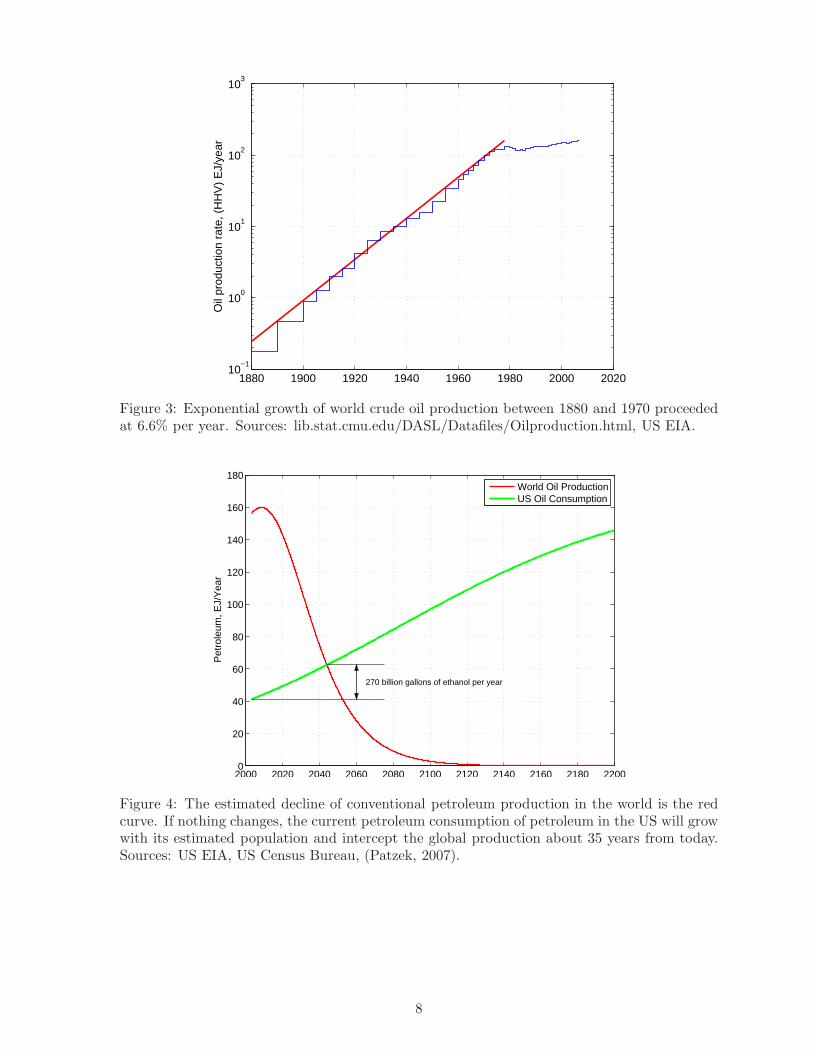
Before peaking2 in 2006, the world production of conventional petroleum grew exponentiallyat 6.6% per year between 1880 and 1970, see Figure 3. The Hubbert curves are symmetrical(Patzek, 2007) and predict world production of conventional petroleum to decline exponentiallyat a similar rate within a decade from now, or so. This decline can be arrested for a while byheroic measures (infill drilling, horizontal wells, enhanced oil recovery methods, etc.), but thelonger it is arrested the more precipitous it will become.

If the current per capita use of petroleum in the US is escalated with the expected growthof US population, the US will have to intercept the entire estimated production of conventionalpetroleum3 in the world by 2042, see Figure 4. In this scenario, the projected increment of USpetroleum consumption between today and 2042 is equivalent to 270 billion gallons of ethanol.

This brings me to the first major conclusion of this paper:

With business as usual there is no long-term solution to the problem of liquid transportationfuel supply for the US alone, much less for the entire world. For this very reason, the USand the rest of the world soon will be on a head-on collision course.

1The US population in 2006.2The short-lived rate peak around 1978 was caused by OPEC limiting its oil production.3I stress again that I am referring to conventional, readily-available petroleum. There will be an offsetting

production from unconventional sources: tar sands, ultra-heavy oil, and natural gas liquefaction, all at very highenergy and environmental costs.

6

1950 1960 1970 1980 1990 20000

5

10

15

20

25

30

35

40

381 billion gallonsof ethanol

Fue

l Hig

h H

eatin

g V

alue

, EJ/

year



Motor GasolineResidual OilDistillate OilAviation FuelEthanol

Figure 1: Currently, the US consumes about 33 times more energy in transportation fuelsthan is necessary to feed its population. This amount of energy is equivalent to 381 billiongallons of ethanol per year. The amount of energy in corn-ethanol is barely visible and itshall always remain so unless we drastically (by a factor of two for starters) lower liquid fuelconsumption. Current consumption of ethanol is about 1.2% of the total fuel consumption(without considering energy inputs to the production system). Source: DOE EIA.

1980 1985 1990 1995 2000 2005 2010 2015 20200

5

10

15

20

25

30

35

Bill

ion

gallo

ns p

er y

ear

Exponential projectionLogistic projectionRFA data2017 − Bush’s Goal

Figure 2: By an exponential extrapolation of ethanol production during the last 7 years at 18.5%per year, one may arrive at 35 billion gallons per year in 2017. The less optimistic logistic fitof the data plateaus at 14 billion gallons per year. Where will the remaining 21 billion gallonsof ethanol come from each year? Sources: DOE EIA, Renewable Fuels Association (RFA).

7

1880 1900 1920 1940 1960 1980 2000 202010

−1

100

101

102

103

Oil

prod

uctio

n ra

te, (

HH

V)

EJ/

year

Figure 3: Exponential growth of world crude oil production between 1880 and 1970 proceededat 6.6% per year. Sources: lib.stat.cmu.edu/DASL/Datafiles/Oilproduction.html, US EIA.

2000 2020 2040 2060 2080 2100 2120 2140 2160 2180 22000

20

40

60

80

100

120

140

160

180

Pet

role

um, E

J/Y

ear

270 billion gallons of ethanol per year

World Oil ProductionUS Oil Consumption

Figure 4: The estimated decline of conventional petroleum production in the world is the redcurve. If nothing changes, the current petroleum consumption of petroleum in the US will growwith its estimated population and intercept the global production about 35 years from today.Sources: US EIA, US Census Bureau, (Patzek, 2007).

8

4 Background

Humans are an integral part of a single system made of all life and all parts of the Earth’snear-surface shown in Figure 5. Thus, as President Vaclav Havel said on July 4, 1994:“Our destiny is not dependent merely on what we do to ourselves but also on what we do for[the Earth] as a whole. If we endanger her, she will dispense with us in the interest of a highervalue – life itself.” So how to proceed?

Top of atmosphere

Empty space

Human existence

Earth

Figure 5: A system defined by the mean Earth surface at Rearth and the top of the atmosphereat Rearth + 100 km, or outer space at Rearth + 400 km. Almost all of human existence occursalong the surface of the blue sphere (edge of the blue circle). As drawn here, the line thicknessactually exaggerates the thickness of the life-giving membrane on which we exist. All radii aredrawn to scale.

It appears that humanity’s survival is subject to these five constraints:

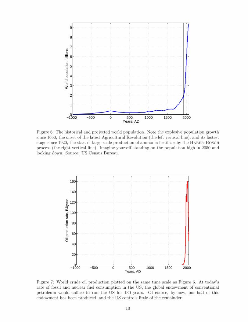
Constraint 1: An almost exponential rate of growth of human population, see Figure 6.

Constraint 2: Too much use of Earth resources; in particular, fossil fuels; and even morespecifically, liquid transportation fuels, see Figure 7.

Constraint 3: The Earth that is too small to feed in perpetuity 7 billion people and counting,1 billion cows, and – now – 1 billion cars, see Figure 8.

Constraint 4: The ossified political structures in which more is better, and more of the sameis also safer.

Constraint 5: A global climate change.

Unfortunately, these five constraints prevent existence of a stable continuous solution tohuman life in the near-future. Alternatively, we may choose from the following two discontinuoussolutions:

Solution 1: Extinguish ourselves and much of the living Earth, or

Solution 2: Fundamentally and abruptly change, while slowly decreasing our numbers.

9

−1000 −500 0 500 1000 1500 20000

1

2

3

4

5

6

7

8

9

Wor

ld p

opul

atio

n, b

illio

ns

Years, AD

Figure 6: The historical and projected world population. Note the explosive population growthsince 1650, the onset of the latest Agricultural Revolution (the left vertical line), and its fasteststage since 1920, the start of large-scale production of ammonia fertilizer by the Haber-Bosch

process (the right vertical line). Imagine yourself standing on the population high in 2050 andlooking down. Source: US Census Bureau.

−1000 −500 0 500 1000 1500 20000

20

40

60

80

100

120

140

160

Oil

prod

uctio

n ra

te, E

J/ye

ar

Years, AD

Figure 7: World crude oil production plotted on the same time scale as Figure 6. At today’srate of fossil and nuclear fuel consumption in the US, the global endowment of conventionalpetroleum would suffice to run the US for 130 years. Of course, by now, one-half of thisendowment has been produced, and the US controls little of the remainder.

10

Figure 8: Human-appropriated (HA) Net Primary Production (NPP) of the Earth. Globalannual NPP refers to the total amount of plant growth generated each year and quantifiedas mass of carbon used to build stems, leaves and roots. Note that in the large portions ofSouth and East Asia, Western Europe, Middle East, and eastern US, humans grab up to 1-2times the net biomass production of local ecosystems. In large cities this ratio increases to 400times. If this present human commandeering of global NPP is augmented with massive agrofuelproduction, the Earth ecosystems will collapse. Source: The Visible Earth, NASA images,06-25-2004, www.nasa.gov/vision/earth/environment/0624−hanpp.html

4.1 Problems with Change

The last time humanity ran mostly on living plant carbon was approximately in 1760. Therewas 1 billion of us, and we certainly knew how to feed ourselves due to the latest AgriculturalRevolution that started in Europe a century earlier (Osborne, 1970). Our food supply problemsthen had to do with political madness, inaptitude, and greed – just as they do today (Davis,2002). Today, however, there is almost 7 times more of us, see Figure 6. We can still feedourselves, but with huge inputs of fossil carbon in addition to fresh plant carbon, minerals, andsoil. These inputs also mine fossil water and pollute surface water, aquifers, the oceans, andthe atmosphere.

By extrapolating human population growth between 1650 and 1920 to 2007, one estimates2.2 billion people, who today could live mostly on plant carbon, but use some coal, oil, andnatural gas. Therefore, it is reasonable to say that today 4.5 billion people4 owe their exis-tence to the Haber-Bosch ammonia process and the fossil fuel-driven, fundamentally unstable“green revolution,” as well as to vaccines and antibiotics. Agrofuels are a direct outgrowth ofthe current “green revolution,” which may be viewed, see Appendix B, as a short-lived butviolent disturbance of terrestrial ecosystems on the Earth.

Since most people have cooked or ridden in a vehicle, many feel empowered to talk aboutenergy as though they were experts. It turns out, however, that issues of energy supply,use, environmental impacts, and – especially – of free energy are too complicated for the adlib homilies we hear every day in the media. Professor Varadaraja Raman, a well-knownphysicist and humanist, said it best: “A major problem confronting society is the lack ofknowledge among the public as to what science is, what constitutes scientific thinking andanalysis, and what science’s criteria are for determining the correctness of statements aboutthe phenomenological world.”

It is a misconception that Constraint 2 can be removed with fresh plant carbon, while

4All global population increase since 1940.

11

Otherlife

Death &Decay

H2O, CO2

Nutrients

PlantMatter

Waste heatWaste heat

Sun energy

“Forever”

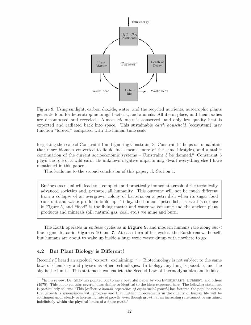
Figure 9: Using sunlight, carbon dioxide, water, and the recycled nutrients, autotrophic plantsgenerate food for heterotrophic fungi, bacteria, and animals. All die in place, and their bodiesare decomposed and recycled. Almost all mass is conserved, and only low quality heat isexported and radiated back into space. This sustainable earth household (ecosystem) mayfunction “forever” compared with the human time scale.

forgetting the scale of Constraint 1 and ignoring Constraint 3. Constraint 4 helps us to maintainthat more biomass converted to liquid fuels means more of the same lifestyles, and a stablecontinuation of the current socioeconomic systems – Constraint 3 be damned.5 Constraint 5plays the role of a wild card. Its unknown negative impacts may dwarf everything else I havementioned in this paper.

This leads me to the second conclusion of this paper, cf. Section 1:

Business as usual will lead to a complete and practically immediate crash of the technicallyadvanced societies and, perhaps, all humanity. This outcome will not be much differentfrom a collapse of an overgrown colony of bacteria on a petri dish when its sugar foodruns out and waste products build up. Today, the human “petri dish” is Earth’s surfacein Figure 5, and “food” is the living matter and water we consume and the ancient plantproducts and minerals (oil, natural gas, coal, etc.) we mine and burn.

The Earth operates in endless cycles as in Figure 9, and modern humans race along shortline segments, as in Figures 10 and 7. At each turn of her cycles, the Earth renews herself,but humans are about to wake up inside a huge toxic waste dump with nowhere to go.

4.2 But Plant Biology is Different!

Recently I heard an agrofuel “expert” exclaiming: “. . . Biotechnology is not subject to the samelaws of chemistry and physics as other technologies. In biology anything is possible, and thesky is the limit!” This statement contradicts the Second Law of thermodynamics and is false.

5In his review, Dr. Silin has pointed out to me a beautiful paper by von Engelhardt, Hubbert, and others(1975). This paper contains several ideas similar or identical to the ideas expressed here. The following statementis particularly salient: “This [collective human experience of exponential growth] has fostered the popular notionthat growth is synonymous with progress and that further improvements in the quality of human life will becontingent upon steady or increasing rate of growth, even though growth at an increasing rate cannot be sustainedindefinitely within the physical limits of a finite earth.”

12

Stock offossil fuels 500 years

Chemicalwaste

Waste heat

Figure 10: A linear process of converting a stock of fossil fuels into waste matter and heatcannot be sustainable. The waste heat is exported to the universe, but the chemical wasteaccumulates. To replenish some of the fossil fuel stock, it will take another 50 to 400 millionyears of photosynthesis, burial, and entrapment.

The rate of entropy production in any natural (irreversible) process, such as photosynthesisor plant growth, is a measure of the dissipation (energy wasted to heat generation) in thatprocess. As observed by Ross and Vlad in their brilliant paper (2005), there exists an old“principle” in the literature (Prigogine, 1945) that says: If a steady state is close enough toequilibrium, the rate of entropy production has an extremum at that state. This “principle”is mathematically correct if and only if thermodynamic fluxes (of mass, heat, etc.) and forces(concentration gradient, temperature gradient, etc.) are proportional and the coefficients ofproportionality form a symmetric matrix (De Groot and Mazur, 1962). Later on, Glansdorff

and Prigogine (1971) restated the “principle” with the thought that close to equilibrium theproportionality between fluxes and forces becomes nearly true: “It is easy to show that if thesteady states occur sufficiently close to equilibrium states they may be characterized by anextremum principle according to which the entropy production has its minimum value at thesteady-state compatible with the prescribed conditions (constraints) to be specified in eachcase.”

Unfortunately this incorrect restatement has been repeated many times, especially in con-nection with biochemical and biological applications, where there is a tendency to present theprinciple of minimum entropy production in even vaguer terms, as a fundamental law of nature,which is supposed to be valid for any evolution equations. For example, (Voet and Voet, 2004)in a widely used text, state that “Ilya Prigogine, a pioneer in the development of irreversiblethermodynamics, has shown that a steady state produces the maximum amount of useful workfor a given energy expenditure under the prevailing conditions. The steady state of an opensystem is therefore its state of maximum thermodynamic efficiency.” This statement is not truein general.

Ross and Vlad (2005) have proven by counterexamples that real systems in arbitrary non-equilibrium states, for example photosynthesizing higher plants or algae, or bacteria, producemore entropy than calculated from the “principles” above. Also, based on Ross and Vlad’sresults, one can show that the losses associated with irreversible heat transfer in a plant dueto an increase of the heat flux from photosynthesis are proportional to the square of this flux.In other words, if the heat-generating photosynthetic activities increase by a factor of two, thecorresponding energy losses must increase by a factor of four. This observation leads to thethird conclusion of this paper:

13

Because of the thermodynamics of irreversible processes, the promises to increase the rateof plant photosynthesis significantly are empty. A higher photosynthetic rate would resultin the disproportionately higher water transpiration fluxes to cool the plants, larger rootsystems, higher respiration rates, and higher overall water requirements of these plants. Itis not a coincidence that – given all contradictory environmental factors – over the last 3.5billion years Mother Nature has fine-tuned plant photosynthesis to its current efficiency.Water, not solar energy conversion, is the real limiting factor of plant efficiency.

5 Plan of Attack

As you are beginning to suspect, it is not sufficient to limit oneself just to discussing liquidtransportation fuels and their future biological sources. These transportation fuels intrudeupon every other aspect of life on the Earth: Availability of clean water to drink and cleanair to breathe, healthy soil and healthy food supply, destruction of biodiversity and essentialplanetary services in the tropics, acceleration of global climate change, and so on.

As with many important policy-making decision processes, I start from the end, here thecellulosic ethanol refineries. This is where most public money, attention, and hope are. Ishow that these refineries are inefficient compared with the existing petroleum- and corn-basedrefineries, and are difficult to scale up.

Then I return to the beginning and show that even if the cellulosic biomass refineries weremarvels of efficiency, they still could not maintain our current lifestyles by a long stretch, simplybecause the Earth will not give us the extra biomass needed to keep on existing as we do. For awhile we might continue to rob this biomass from the poor tropics, but the results are alreadydisastrous for all humanity, see Figure 11.

Figure 11: In the fall of 1997, an orgy of 176 fires in Indonesia burned 12 million ha of virginforest and generated as much greenhouse gases as the US in one year. 133 of these illegal fireswere started by oil palm plantation/logging companies to steal old-growth trees and burn therest for new plantations. The smoke and ozone plume had global extent. Sources: NASA’sEarth Probe Total Ozone Mapping, Spectrometer (TOMS), October 22, 1997; (Schimel andBaker, 2002; Page et al., 2002; Patzek and Patzek, 2007).

14

Once I have demonstrated the utter impossibility of replacing liquid transportation fuelswith agrofuels and conveyed the damage to the planet their production is causing now, I proposea positive solution that involves photovoltaics and batteries.

6 Efficiency of Cellulosic Ethanol Refineries

I start from a “reverse-engineering” calculation of energy efficiency of cellulosic ethanol pro-duction in an existing Iogen pilot plant, Ottawa, Canada. I then discuss the inflated energyefficiency claims of five out-of-six recipients of $385 millions of DOE grants to develop cellulosicethanol refineries.

6.1 Iogen Ottawa Facility

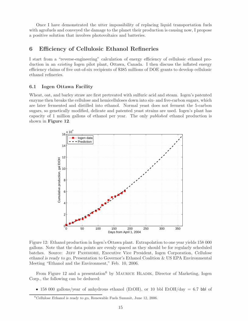
Wheat, oat, and barley straw are first pretreated with sulfuric acid and steam. Iogen’s patentedenzyme then breaks the cellulose and hemicelluloses down into six- and five-carbon sugars, whichare later fermented and distilled into ethanol. Normal yeast does not ferment the 5-carbonsugars, so genetically modified, delicate and patented yeast strains are used. Iogen’s plant hascapacity of 1 million gallons of ethanol per year. The only published ethanol production isshown in Figure 12.

0 50 100 150 200 250 300 3500

2

4

6

8

10

12

14

16x 10

4

Days from April 1, 2004

Cum

ulat

ive

prod

uctio

n, g

al E

tOH

Iogen dataPrediction

Figure 12: Ethanol production in Iogen’s Ottawa plant. Extrapolation to one year yields 158 000gallons. Note that the data points are evenly spaced as they should be for regularly scheduledbatches. Source: Jeff Passmore, Executive Vice President, Iogen Corporation, Cellulose

ethanol is ready to go, Presentation to Governor’s Ethanol Coalition & US EPA EnvironmentalMeeting “Ethanol and the Environment,” Feb. 10, 2006.

From Figure 12 and a presentation6 by Maurice Hladik, Director of Marketing, IogenCorp., the following can be deduced:

• 158 000 gallons/year of anhydrous ethanol (EtOH), or 10 bbl EtOH/day = 6.7 bbl of

6Cellulose Ethanol is ready to go, Renewable Fuels Summit, June 12, 2006.

15

equivalent gasoline/day were actually produced. In press interviews, Iogen claims to beproducing 790 000 gallons of ethanol7 per year.

• There exists 2 × 52000 = 104000 gallons of fermentation tank volume.

• The actual ethanol production and tank volume give the ratio of 1.5 gallons of ethanolper gallon of fermenter and per year.

• I assume 7-day batches + 2-day cleanups.

• Thus, there is ca. 4% of alcohol in a batch of industrial wheat-straw beer, in contrast to12 to 16% of ethanol in corn-ethanol refinery beers.

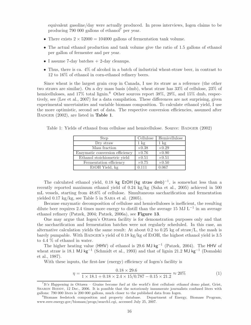
Since wheat is the largest grain crop in Canada, I use its straw as a reference (the othertwo straws are similar). On a dry mass basis (dmb), wheat straw has 33% of cellulose, 23% ofhemicelluloses, and 17% total lignin.8 Other sources report 38%, 29%, and 15% dmb, respec-tively, see (Lee et al., 2007) for a data compilation. These differences are not surprising, givenexperimental uncertainties and variable biomass composition. To calculate ethanol yield, I usethe more optimistic, second set of data. The respective conversion efficiencies, assumed afterBadger (2002), are listed in Table 1.

Table 1: Yields of ethanol from cellulose and hemicellulose. Source: Badger (2002)

Step Cellulose HemicelluloseDry straw 1 kg 1 kg

Mass fraction ×0.38 ×0.29Enzymatic conversion efficiency ×0.76 ×0.90

Ethanol stoichiometric yield ×0.51 ×0.51Fermentation efficiency ×0.75 ×0.50

EtOH Yield, kg 0.111 0.067

The calculated ethanol yield, 0.18 kg EtOH (kg straw dmb)−1, is somewhat less than arecently reported maximum ethanol yield of 0.24 kg/kg (Saha et al., 2005) achieved in 500mL vessels, starting from 48.6% of cellulose. Simultaneous saccharification and fermentationyielded 0.17 kg/kg, see Table 5 in Saha et al. (2005).

Because enzymatic decomposition of cellulose and hemicelluloses is inefficient, the resultingdilute beer requires 2.4 times more energy to distill than the average 15 MJ L−1 in an averageethanol refinery (Patzek, 2004; Patzek, 2006a), see Figure 13.

One may argue that Iogen’s Ottawa facility is for demonstration purposes only and thatthe saccharification and fermentation batches were not regularly scheduled. In this case, analternative calculation yields the same result: At about 0.2 to 0.25 kg of straw/L, the mash isbarely pumpable. With Badger’s yield of 0.18 kg/kg of EtOH, the highest ethanol yield is 3.5to 4.4 % of ethanol in water.

The higher heating value (HHV) of ethanol is 29.6 MJ kg−1 (Patzek, 2004). The HHV ofwheat straw is 18.1 MJ kg−1 (Schmidt et al., 1993) and that of lignin 21.2 MJ kg−1 (Domalskiet al., 1987).

With these inputs, the first-law (energy) efficiency of Iogen’s facility is

η =0.18 × 29.6

1 × 18.1 + 0.18 × 2.4 × 15/0.787 − 0.15 × 21.2≈ 20% (1)

7It’s Happening in Ottawa – Grains become fuel at the world’s first cellulosic ethanol demo plant, Grist,Sharon Boddy, 12 Dec., 2006. It is possible that the notoriously innumerate journalists confused liters withgallons: 790 000 liters is 200 000 gallons, much closer to the published data from Iogen.

8Biomass feedstock composition and property database. Department of Energy, Biomass Program,www.eere.energy.gov/biomass/progs/search1.cgi, accessed July 25, 2007.

16

0 5 10 150

5

10

15

20

25

30

Volume % of Ethanol in Water

Kgs

of S

team

/Gal

lon

Anh

ydro

us E

tOH

TheoreticalPracticalIogen Demand

Figure 13: Steam requirement in ethanol beer distillation. The 3.7% beer requires 2.4 timesmore steam than a 12% beer. Source (Jacques et al., 2003).

where the density of ethanol is 0.787 kg L−1 and the entire HHV of lignin was used to offsetdistillation fuel (another optimistic assumption for the wet separated lignin). This calculationdisregards the energy costs of high-pressure steam treatments of the straw at 120 or 140 0C,and the separated solids at 190 0C, sulfuric acid and sodium hydroxide production, etc. Also,the complex enzyme production processes must use plenty of energy.

This analysis leads to the fourth conclusion:

The Iogen plant in Ottawa, Canada, has operated well below name plate capacity forthree years. Iogen should retain their trade secrets, but in exchange for the significant sub-sidies from the US and Canadian taxpayers they should tell us what the annual productionof alcohols was, how much straw was used, and what the fossil fuel and electricity inputswere. The ethanol yield coefficient in kg of ethanol per kg straw dmb is key to public assess-ments of the new technology. Similar remarks pertain to the Novozymes projects heavilysubsidized by the Danes. Until an existing pilot plant provides real, independently verifieddata on yield coefficients, mash ethanol concentrations, etc., all proposed cellulosic ethanolrefinery designs are speculation.

6.2 Proposed Cellulosic Ethanol Refineries

Now I present at face value the stated energy efficiencies9 of the six proposed10 cellulosic ethanolplants awarded 385 million USD by the US Department of Energy.

Figure 14 ranks the rather imaginary claims of 5 out of 6 award recipients. For calibration,after 87 years of development and optimization, the actual energy efficiency of Sasol’s Fischer-

Tropsch coal-to-liquid fuels plants is about 42% (Steynberg and Nel, 2004). The average

9The HHV of ethanol out divided by the HHV of biomass in. No fossil fuels inputs into the plants and theraw materials they use are accounted for.

10Environmental and Energy Study Institute, 122 C STREET, N.W., SUITE 630 WASHINGTON, D.C.,20001, www.eesi.org/publications/Press%20Releases/2007/2-28-07

−doe

−biorefinery

−awards.pdf

17

0 20 40 60 80 100

Abengoa Bioenergy Biomass of KS

Iogen Bioref. Partners, of Arlington, VI

BlueFire Ethanol, Inc. of Irvine, CA

ALICO, Inc. of LaBelle, FL

Broin Companies of Sioux Falls, SD

Range Fuels of Broomfield, CO

Energy efficiency, %

Iogen Ottawa plantAvg.corn ethanol refineryPerlack et al. (2005)Avg petroleum refinery

Figure 14: Stated energy efficiencies of the six future cellulosic ethanol refineries awarded $385millions in DOE grants. The calculated energy efficiency (left line) of an existing cellulosicethanol refinery in Ottawa serves to calibrate the rather inflated efficiency claims of 5/6 grantrecipients. Energy efficiencies of an average ethanol refinery and petroleum refinery (Patzek,2006a) are also shown (second and last line from the left).

energy efficiency of the highly optimized corn ethanol refineries is 37% (not counting graincoproducts as fuels). An average petroleum refinery is about 88% energy-efficient.11 For details,see (Patzek, 2006b; Patzek, 2006c; Patzek, 2006a). The DOE/USDA report by Perlack et al.(2005) has led to the claims by an influential venture capitalist, Mr. Vinod Khosla (2006),of being able to produce 130 billion gallons of ethanol from 1.4 billion tons of biomass (dmb),apparently at a 52% thermodynamic efficiency.

To see how very different the new fossil-energy-free world will be, let’s compare power fromIogen’s plant with that from an oil well in the US. Ever more power is what we must haveto continue our current way of life (cf. Footnote 5). Iogen’s plant delivers the power of 7barrels of oil per day (68 kW). Average power of petroleum wells in the largely oil-depleted USwas 10 bbl (well-day)−1 in 200612 (98 kW). Therefore, an average US petroleum well deliversmore power than a city-block size Iogen facility in Ottawa and its area of straw collection,probably 50 km in radius, which at this time is saturated with fossil fuels outright and theirproducts (ammonia fertilizers, field chemicals, roads, etc.). The petroleum well also uses littleinput power; unfortunately, soon petroleum will not be a transportation option. Such is thedifference between solar energy stocks (depletable fossil fuels) and flows (daily photosynthesis).

One can calculate that an average agricultural worker in the US uses 800 kW of fossil energyinputs and outputs 3000 kW. An average oil & gas worker in California uses 2800 kW of fossilenergy inputs and outputs 14,500 kW. Due to fossil energy and machines these two workers aresupermen, each capable of doing the work of 8000 and 28000 ordinary humans, respectively.These two fellows are about to become human again, and we need to get used to this idea.

11As pointed out by Drs. John Benemann and John Newman, this comparison may be unfair. No liquidfuel technology will ever match petroleum refining, but petroleum-derived fuels will not last for very long.

12See www.eia.doe.gov/emeu/aer/txt/ptb0502.html, accessed July 25, 2007.

18

Now, you may want to go back to Section 4.1 and reread it.

7 Where Will the Agrofuel Biomass Come From?

Collectively, the EU and the US have spent billions of dollars to be able to construct the ineffi-cient behemoth factories, which in the distant future might ingest megatonnes or gigatonnes ofapparently free biomass “trash” and spit out priceless liquid transportation fuels. It is there-fore prudent to ask the following question: Where, how much, and for how long will the Earthproduce the extra biomass to quench our unending thirst to drive 1 billion cars and trucks?

The answer to this question is immediate and unequivocal: Nowhere, close to nothing, andfor a very short time indeed. On the average, our planet has zero excess biomass at her disposal.

7.1 Useful Terminology

Several different ecosystem13 productivities, i.e., measures of biomass accumulation per unitarea and unit time have been used in the ecological literature, e.g., (Reichle et al., 1975; Ran-derson et al., 2001) and many others. Usually this biomass is expressed as grams of carbon(C) per square meter and per year, or as grams of water-free biomass (dmb) per square meterand year.14 The conversion factor between these two estimates is the carbon mass fraction inthe fundamental building blocks of biomass, CHxOy, where x and y are real numbers, e.g., 1.6and 0.6, that express the overall mass ratios of hydrogen and oxygen to carbon. The followingdefinitions are common in ecology:

1. Gross Primary Productivity, GPP = mass of CO2 fixed by plants as glucose.

2. Ecosystem respiration, Re = mass of CO2 released by metabolic activity of autotrophs,Ra, and heterotrophs (consumers and decomposers), Rh:

Re = Ra + Rh (2)

where decomposers are defined as worms, bacteria, fungi, etc. Plants respire about 1/2of the carbon available from photosynthesis after photorespiration, with the remainderavailable for growth, propagation, and litter production, see (Ryan, 1991). Heterotrophsrespire most, 82 to 95%, of the biomass left after plant respiration (Randerson et al.,2001).

3. Net Primary Productivity, NPP = GPP − Ra.

4. Net Ecosystem Productivity

NEP = GPP - Re - Non-R sinks and flows (3)

The older NEP definitions would usually neglect the non respiratory losses, e.g., (Reichleet al., 1975). All ecological definitions of NEP I have seen, lump incorrectly mass flowsand mass sources and sinks, calling them “fluxes,” see, e.g., (Randerson et al., 2001; Lugoand Brown, 1986). For more details, see Appendix B.

The typical net primary productivities of different ecosystems are listed in Appendix C.

13An ecosystem is defined in more detail in Appendix A.14Or as kilograms (dmb) of biomass per hectare and per year.

19

−600 −500 −400 −300 −200 −100 040

60

80

100

120

140

160

180

2005 world soybean crop

2005 US soybean cropCar

bon

buria

l, M

ega

tonn

es d

ry b

iom

ass/

yr

Time, MYr

Figure 15: Plot of global organic carbon burial during the Phanerozoic eon. Carbon burialrate modified from Berner (2001; 2003). The units of carbon burial have been changed from1018 mol C Myr−1 to Mt biomass yr−1. The very high carbon burial values centered around 300Myr ago are due predominantly to terrestrial carbon burial and coal formation. Most plantshave been buried in swamps, shallow lakes, estuaries, and shallow coastal waters. Note thathistorically the average rate of carbon burial on the Earth has been tiny, half-way between theUS- and world crops of soybeans in 2005. This burial rate amounts to 120 × 106/110 × 109

×

100% = 0.1% of global NPP of biomass.

7.2 Plant Biomass Production

The reason for the Earth recycling all of her material parts can be explained by looking againat Figure 5. The Earth is powered by the sun’s radiation that crosses the outer boundary of heratmosphere and reaches her surface. The Earth can export into outer space long-wave infraredradiation.15 But, because of her size, the Earth holds on to all mass of all chemical elements,except perhaps for hydrogen. By maintaining an oxygen-rich atmosphere, life has managed toprevent the airborne hydrogen from escaping Earth’s gravity by reacting it back to water (anddestroying ozone).

If all mass must stay on the Earth, all her households must recycle everything; otherwiseinternal chemical waste would build up and gradually kill them. Mother Nature does notusually do toxic waste landfills and spills.

In a mature ecosystem, one species’ waste must be another species’ food and no net wasteis ever created, see Figure 9. The little imperfections in the Earth’s surface recycling programshave resulted in the burial of a remarkably tiny fraction of plant carbon in swamps, lakes, andshallow coastal waters16, see Figure 15. Very rarely the violent anoxic events would kill mostof life in the oceanic waters and cause faster carbon burial. Over the last 460,000,000 years (and

15Therefore, the Earth is an open system with respect to electromagnetic radiation. Life could emerge on herand be sustained for 3.5 eons because of this openness.

16Much of this burial has been eliminated by humans. We have paved over most of the swamps and destroyedmuch of the coastal mangrove forests, the highest-rate local sources of terrestrial biomass transfer into seawater.

20

going back all the way to 2,500,000,000 years ago), the Earth has gathered and transformedsome of the buried ancient plant mass into the fossil fuels we love and loath so much.

0 100 200 300 400 500 600−0.5

0

0.5

1

1.5

2

2.5

Age, years

kg/

m 2 −

yr

NPPR

h

NEP

Figure 16: Forest ecosystem biomass fluxes simulated for a typical stand in the H. J. Andrews

Experimental Forest. The Net Primary Productivity (NPP), the heterotrophic respiration (Rh),and the Net Ecosystem Productivity (NEP) are all strongly dependent on stand age. Thisparticular stand builds more plant mass than heterotrophs consume for 200 years. After that,for any particular year, an old-growth stand is in equilibrium and its average net ecosystemproductivity is zero. Adapted from Songa & Woodcock (2003).

The proper mass balance of carbon fluxes in terrestrial ecosystems, see Appendix B,confirms the compelling thermodynamic argument that sustainability of any ecosystem requiresall mass to be conserved on the average. The larger the spatial scale of an ecosystem and thelonger the time-averaging scale are, the stricter adherence to this rule must be. Such are thelaws of nature.

Physics, chemistry and biology say clearly that there can be no sustained net mass outputfrom any ecosystem for more than a few years. A young forest in a temperate climate growsfast in a clear-cut area, see Figure 16, and transfers nutrients from soil to the young trees.The young trees grow very fast (there is a positive NPP), but the amount of mass accumulatedin the forest is small. When a tree burns or dies some or most of its nutrients go back to thesoil. When this tree is logged and hauled away, almost no nutrients are returned. After loggingyoung trees a couple of times the forest soil becomes depleted, while the populations of insectsand pathogens are well-established, and the forest productivity rapidly declines (Patzek andPimentel, 2006). When the forest is allowed to grow long enough, its net ecosystem productivitybecomes zero on the average.

Therefore, in order to export biomass (mostly water, but also carbon, oxygen, hydrogenand a plethora of nutrients) an ecosystem must import equivalent quantities of the chemicalelements it lost, or decline irreversibly. Carbon comes from the atmospheric CO2 and waterflows in as rain, rivers and irrigation from mined aquifers and lakes. The other nutrients,however, must be rapidly produced from ancient plant matter transformed into methane, coal,petroleum, phosphates17, etc., as well as from earth minerals (muriate of potash, dolomites,

17Over millions of years, the annual cycles of life and death in ocean upwelling zones have propelled sedimenta-tion of organic matter. Critters expire or are eaten, and their shredded carcasses accumulate in sediments as fecal

21

etc.), – all irreversibly mined by humans. Therefore, to the extent that humans are no longerintegrated with the ecosystems in which they live, they are doomed to extinction by exhaustingall planetary stocks of minerals, soil and clean water. The question is not if, but how fast?

It seems that with the exponentially accelerating mining of global ecosystems for biomass,the time scale of our extinction is shrinking with each crop harvest. Compare this statementwith the feverish proclamations of sustainable biomass and agrofuel production that flood usfrom the confused media outlets, peer-reviewed journals, and politicians.

7.3 Is There Any Other Proof of NEP = 0?

I just gave you an abstract proof of no trash production in Earth’s Kingdom, except for itsdirty human slums.

Are there any other, more direct proofs, perhaps based on measurements? It turns out thatthere are two approaches that complement each other and lead to the same conclusions. Thefirst approach is based on a top-down view of the Earth from a satellite and a mapping of thereflected infrared spectra into biomass growth. I will summarize this proof here. The secondapproach involves a direct counting of all crops, grass, and trees, and translating the weighedor otherwise measured biomass into net primary productivity of ecosystems. Both approachesyield very similar results.

0 1 2 3 4 5

Asia Pacific

South America

North America

Europe

NPP relative to North America

Figure 17: NPP’s of Asia-Pacific, South America, and Europe – relative to North America.Source: MOD17A2/A3 model.

pellets and as gelatinous flocs termed marine snow. Decay of some of this deposited organic matter consumesvirtually all of the dissolved oxygen near the seafloor, a natural process that permits formation of finely-layered,organic-rich muds. These muds are a biogeochemical “strange brew,” where calcium – derived directly fromseawater or from the shells of calcareous plankton – and phosphorus – generally derived from bacterial decayof organic matter and dissolution of fish bones and scales – combine over geological time to form pencil-thinlaminae and discrete sand to pebble-sized grains of phosphate minerals. Source: Grimm (1998).

22

7.4 Satellite Sensor-based Estimates

Global ecosystem productivity can be estimated by combining remote sensing with a carboncycle analysis. The US National Aeronautics and Space Administration (NASA) Earth Observ-ing System (EOS) currently “produces a regular global estimate of gross primary productivity(GPP) and annual net primary productivity (NPP) of the entire terrestrial earth surface at1-km spatial resolution, 150 million cells, each having GPP and NPP computed individually”(Running et al., 2000). The MOD17A2/A3 User’s Guide (Heinsch and et al., 2003) provides adescription of the Gross and Net Primary Productivity estimation algorithms (MOD17A2/A3)designed for the MODIS18 sensor.

The sample calculation results based on the MOD17A2/A3 algorithm are listed in Table 2.The NPPs for Asia Pacific, South America, and Europe, relative to North America, are shown inFigure 17. The phenomenal net ecosystem productivity of Asia Pacific is 4.2 larger than thatof North America. The South American ecosystems deliver 2.7 times more than their NorthAmerican counterparts, and Europe just 0.85. It is no surprise then that the World Bank19, aswell as agribusiness and logging companies – Archer Daniel Midlands (ADM), Bunge, Cargill,Monsanto, CFBC, Safbois, Sodefor, ITB, Trans-M, and many others – all have moved in forceto plunder the most productive tropical regions of the world, see Figure 18.

The final result of this global “end-game” of ecological destruction will be an unmitigatedand lightening-fast collapse of ecosystems protecting a large portion of humanity.20

Table 2: Version 4.8 NPP/GPP global sums (posted: 01 Feb 2007)a

Yearb GPP (Pg C/yrc) NPPd (Pg C/yr)

2000 111 53

2001 111 53

2002 107 51

2003 108 51

2004 109 52

2005 108 51

aNumerical Terradynamic Simulation Group, The University of Montana, Missoula, MT 59812, im-ages.ntsg.umt.edu/index.php.b2000 and 2001 were La Nina years, and 2002 and 2003 were weak El Nino years.c1 Pg C = 1 peta gram of carbon = 1015 grams = 1 billion tonnes = 1 Gt of carbon. 50 Gt of carbonper year is equivalent to 1800 EJ yr−1.dThis represents all above-ground production of living plants and their roots. Humans cannot dig up allthe roots on the Earth, so effectively ∼1/2 NPP might be available to humans if all other heterotrophsliving on the Earth stopped eating.

18MODIS (or Moderate Resolution Imaging Spectroradiometer) is a key instrument aboard the Aqua and Terra

satellites. The MODIS instrument provides high radiometric sensitivity (12 bit) in 36 spectral bands ranging inwavelength from 0.4 to 14.4 µm. MODIS provides global maps of several land surface characteristics, includingsurface reflectance, albedo (the percent of total solar energy that is reflected back from the surface), land surfacetemperature, and vegetation indices. Vegetation indices tell scientists how densely or sparsely vegetated a regionis and help them to determine how much of the sunlight that could be used for photosynthesis is being absorbedby the vegetation. Source: modis.gsfc.nasa.gov/about/media/modis

−brochure.pdf.

19Source: (Anonymous, 2007). The World Bank through its huge loans is behind the largest-ever destructionof tropical forest in the equatorial Africa.

20For example, in the next 20 years, Australia may gain another 100 million refugees from the depletedIndonesia; look at Haiti for the clues.

23

Figure 18: Hundreds of fires were burning in the Democratic Republic of Congo and Angola onDec 16, 2005 (top), and Aug 11, 2006 (bottom). Most of the fires are set by humans to clearland for farming, rangelands, and industrial biomass plantations. In this way, vast areas of thecontinent are being irreversibly transformed. Source: Satellite Aqua, 2 km pixels size. Imagescourtesy MODIS Land Rapid Response Team at NASA.

24

Jan Feb Mar Apr May Jun Jul Aug Sep Oct Nov Dec0

2

4

6

8

10

12

14

16

18

20

NP

P H

HV

, EJ/

mon

th

MeanMedian

Figure 19: A MOD17A2/A3-based calculation of US NPP in the year 2003. Monthly data forthe mean and median GPP were acquired from images.ntsg.umt.edu/browse.php. The land areaof the 48 contiguous states plus the District of Columbia = 7444068 km2. Conversion to higherheating values (HHV) was performed assuming 17 MJ kg−1 dmb biomass. Conversion from kgC to kg biomass was 2.2, see Footnote b in Table 10 in Appendix C. NPP = 0.47 × GPP for2003. The robust median productivity estimate of the 2003 US NPP is 90 EJ yr−1.

7.5 NPP in the US

The overall median values of net primary productivity may be converted to the higher heatingvalue (HHV) of NPP in the US, see Figure 19. In 2003, thus estimated net annual biomassproduction in the US was 5.3 Gt and its HHV was 90 EJ. One must be careful, however, becausethe underlying distributions of ecosystem productivity are different for each ecosystem andhighly asymmetric. Therefore, lumping them together and using just one median value canlead to a substantial systematic error. For example, the lumped value of US NPP of 90 EJ,underestimates the overall 2003 estimate21 of 0.408×7444068×106

×17×106×2.2×10−18 = 113

EJ by some 20%.To limit this error, one can perform a more detailed calculation based on the 16 classes

of land cover listed in Table 2 in (Hurtt et al., 2001). The MODIS-derived median NPPs arereported for most of these classes. The calculation inputs are shown in Table 3. Since thespatial set of land-cover classes cannot be easily mapped onto the administrative set of USDAclasses of cropland, woodland, pastureland/rangeland, and forests, Hurtt et al. (2001) providean approximate linear mapping between these two sets, in the form of a 16 × 4 matrix ofcoefficients between 0 and 1. I have lumped the land-cover classes somewhat differently (to becloser to USDA’s classes), and the results are shown in Table 4 and Figure 20.

The Cropland + Mosaic class here comprises the USDA’s cropland, woodland, and someof the pasture classes. The Remote Vegetation class comprises some of the USDA’s rangelandand pastureland classes. The USDA forest class is somewhat larger than here, as some of thesmaller patches of forest, such as parks, etc., are in the Mosaic class. Thus calculated 2003US NPP is 118 EJ yr−1, 74 EJ yr−1 of above-ground (AG) plant construction and 44 EJ yr−1 inroot construction. In addition 12/74 = 17% of AG vegetation is in remote areas, not counting

21The median 2003 US NPP of 0.408 kg C m−2 yr−1 was posted at images.ntsg.umt.edu/browse.php.

25

Table 3: The 2003 US NPP by ground cover class

Classa Areaa 2003 US NPPb Root:shootc

106 ha 106 t ha−1 yr−1

1 Cropland+Mosaicd 219 893 0.318

2 Grassland 123 603 4.224

3 Mixed forest 38 1159 0.456

4 Woody savannahe 33 1694 0.642

5 Open shrublandf 124 620 1.063

6 Closed shrublandg 3 966 1.063

7 Deciduous broadleaf forest 95 1153 0.456

8 Evergreen needleleaf forest 118 1153 0.403

aTable 2 in (Hurtt et al., 2001).bNumerical Terradynamic Simulation Group, The University of Montana, Missoula, MT 59812, im-ages.ntsg.umt.edu/index.php.cTable 2 in (Mokany et al., 2006).dLands with a mosaic of croplands, forests, shrublands and grasslands in which no one component coversmore than 60% of the landscape.eHerbaceous and other understory systems with forest canopy cover over 30 and 60%.fWoody vegetation with less than 2 m tall and with shrub cover 10 to 60%.gWoody vegetation with less than 2 m tall and with shrub cover > 60%.

Table 4: The 2003 US NPP by lumped ground cover classes

Classa Areaa 2003 US NPPb HHVc

106 ha 106 t ha−1 yr−1 EJ yr−1

1 Cropland+Mosaic 219 1484.8 25.2

2 Pastures 123 142.3 2.4

3 Remote vegetationd 160 724.1 12.3

4 Foreste 252 2030.0 34.5

5 Rootsf 754 2575.0 43.8

aDerived from Table 2 in (Hurtt et al., 2001) and USDA classesbIn classes 1 – 4, only above-ground biomass is reported. Class 5 lumps all the roots. The calculationshere are based on Table 3 with the multiplier of 2.2 to convert from carbon to biomass.c The higher heating value with 17 MJ kg−1 on the average.d Classes 4 + 5 + 6 in Table 3.eClasses 3 + 7 + 8 in Table 3.fNote that roots comprise 44/74 = 59% of NPP. Also the land cover classes here account for 97% of USland area.

the remote forested areas. Note that my use of land-cover classes and their typical root-to-shoot ratios yields an overall result (118 EJ yr−1) which is very similar to that derived by theNumerical Terradynamic Simulation Group (113 EJ yr−1).

Therefore, the DOE/USDA proposal to produce 130 billion gallons of ethanol from 1400million tonnes of biomass (Perlack et al., 2005) each year – and year-after-year –, would consume32% of the remaining above-ground NPP in the US, see Figure 20, if one assumes a 52% energy-efficiency of the conversion.22 At the current 26% overall efficiency of the corn-ethanol cycle

22As I mentioned before, this efficiency is close to the theoretical thermodynamic efficiency of the Fischer-

Tropsch process never practically achieved with coal, let alone biomass. After 87 years of research and produc-

26

Nuclear

Natural Gas

Coal

Crude Oil

BiomassHydro

Primary Energy Use

105 EJ/yr

Roots

Remote vegetation

Forest

Cropland+Mosaic

Pastures

NPP118 EJ/yr

Biomass for agrofuels

1.4 or 2.8 Gt/yr

Current corn ethanol

Perlack Report

0

-44

100

25

50

75

-25

EJ/yr

Figure 20: Primary energy consumption and net primary productivity (NPP) in the US in 2003.The annual growth of all biomass in the 48 contiguous states plus the District of Columbia hasbeen translated from gigatonnes per year to the higher heating value of this biomass growthin exajoules per year. The USDA/DOE proposal (Perlack et al., 2005) to produce 130 billiongallons of ethanol per year from 1.4 billion tonnes of biomass would consume 32% of above-ground NPP in the US at a 52% conversion efficiency, or 64% at the current efficiency of thecorn-ethanol cycle (Patzek, 2006a). Sources: EIA, Numerical Terradynamic Simulation Group,and (Patzek, 2007).

(Patzek, 2006a), roughly 64% of all AG NPP in the US would have to be consumed to achievethis goal with zero harvest losses.23 To use more than half of all accessible above-ground plantgrowth in all forests, rangeland, pastureland and agriculture in the US to produce agrofuelswould be a continental-scale ecologic and economic disaster of biblical proportions.24

tion experience, current F-T coal plants achieve a 42% efficiency, see, e.g., (Steynberg and Nel, 2004).23In forestry, roughly 1/2 of AG biomass is exported as tree logs; the rest is lost and burned.24We are moving swiftly down this merry path: “Green Energy Resources traveled to Florida and Georgia

this week to procure upwards of a million tons of forest fire timber from the region at no cost to the company.The timber is valued at approximately $15-20 million. Green Energy Resources plans to use the wood to supplybiomass power plants in the United States as well as for exports.” Source: Green Energy Resources, May 23,2007, Press Release. Accessed on June 21, 2007.

27

8 Photovoltaic Cells vs. Agrofuels

It seems that we will do anything to keep on driving our cars. Therefore, the proper questionto ask is this: How much continuous motive power can be extracted from 1 m2 of land surfaceoccupied by photovoltaic cells, wind turbines, or major energy crops: corn, sugarcane, acacias,and eucalypts? For comparison, I also use 1 m2 of land overlying a medium-quality oil fieldproduced at a constant rate to deliver automotive fuels. For each renewable energy source, Icalculate an extra land area necessary to recover all free-energy costs of producing an auto-motive fuel or electricity. Similarly, I charge the oil field with all energy costs of recoveringoil, transporting it to refineries, processing to gasoline and/or diesel fuel, and transporting thefinished automotive fuels from the refineries to service stations.25 I spend the generated auto-motive power on driving an efficient internal-combustion engine car, such as the Toyota Priusor a diesel engine car, and an all-electric battery car.

8.1 General Comparisons

I start from the ancient solar energy stored in a medium-to-good quality oil reservoir. I assumethat this reservoir is produced at a constant average rate over 20 – 30 years and 100 W m−2 ofprimary power is drawn from it continuously. This amount of power is rather small comparedwith prolific oil fields, which can develop 200 to 400 W m−2 for years. The only problem withmy oil reservoir is that this resource is finite and irreplaceable and after 30 years there is noproducible oil left in it.

One m2 of horizontal photovoltaic cell panels may generate 15% of the average26 US inso-lation of 200 W, i.e., 30 W of electricity continuously.27 I also assume that photovoltaic cellassemblies effectively occupy twice the area of the panels.

One m2 of land occupied by wind turbines may produce continuously 1 W of electricity(Hayden, 2002).

One m2 of land occupied by agrofuel plantations may produce continuously 0.07 to 0.40W m−2 as transportation fuels. All systems are compared in Figure 21. Only the renewablesystems are compared in Figure 22.

8.2 US corn-ethanol system

The Second Law analysis of the US corn-ethanol system is based on the calculations summarizedin Figure 23 and Table 5 (Patzek, 2004). The average corn grain harvest was assumed tobe 8600 kg ha−1, below the all-time record yield of 10000 kg ha−1 in 2004. The ethanol plantswere assumed to operate at 92% of theoretical efficiency. The net-free energy ratio28 of the UScorn grain-ethanol system is 0.24/(0.13+0.19) = 0.77, see Table 5. Notice that the Second Lawanalysis here cannot be translated into an equivalent net-energy ratio used in the nonphysicaland incomplete analyses by DOE and USDA (see Patzek (2006a) for more information).

8.3 Acacia-for-energy system

The exceptionally prolific stand of Acacia mangium trees in Figure 24, captures solar energy atthe rate of 1.39 W/m2 as stemwood+bark, and 0.31 W/m2 as slash, which is usually destroyedby burning. Twenty percent of the stemwood mass is lost in harvest, handling, and processing.Again, we do not want to just burn the wood, but we convert its free energy to electricityand/or automotive fuels. For the three scenarios discussed in Patzek & Pimentel (2006),

25The substantial fuel transportation and blending costs are not included for biofuels.26The 24-hour, 365-day average insolation of a flat horizontal surface anywhere in the US varies between 125

and 375 W m−2 (3 to 9 kWh m−2 day−1), and is almost exactly 200 W m−2 on the average.27Of course free energy is also used to produce solar cells. The life-cycle analysis of solar cells will be performed

later.28An extension of the popular but inadequate measure of efficiency of energy systems (Patzek, 2006a).

28

0 20 40 60 80 100

Eucalypt Ethanol

Corn Stover Ethanol

Eucalypt FT Fuel

Eucalypt Electricity

Corn Grain Ethanol

Acacia Ethanol

Acacia FT Fuel

Sugarcane Ethanol

Acacia+Electricity

Wind turbine

PV Cell

Oilfield

Captured Sun−Power, Primary W/m 2

Figure 21: From the top: Ancient solar power extracted from 1 m2 of a medium-quality oilreservoir by producing its crude oil for 30 years at a constant rate; continuous solar powercaptured by a 15 W m−2 horizontal photovoltaic cell panel converted to primary energy bymultiplying it by 2.43 (the assumed ratio of efficiencies of an all-electric car to a 40 mpg ICcar); continuous primary power of a 1 W m−2 wind turbine; continuous solar power captured byA. mangium, Brazilian sugarcane, US corn, and E. deglupta and converted to various primaryenergy sources, mostly agrofuels. Note that the specific amounts of power outputs of theseplant-energy systems are almost invisible at this scale.

Table 5: Solar power capture, free energy consumption, and free energy output by US cornfield-ethanol distillery systems (Patzek, 2004)

Quantity Power UnitsGrain capture 0.44 W/m2

Stem/leaves capturea 0.46 W/m2

CExCb in corn production 0.13 W/m2

CExC in ethanol production 0.19 W/m2

Grain ethanol capturec 0.24 W/m2

Stover Ethanol capturec 0.10 W/m2

60%-efficient fuel cell outputd 0.15 We/m2

35%-efficient IC engine output 0.09 W/m2

aAbbreviated as stover. 75% of corn stover is collected from the fields, a long-term environmental calamity.bThe cumulative free energy (exergy) consumption, CExC, is equal the minimum work of reversible restoration of theplantation ecosystem and its energy input sources.cOnly for comparison. Fuel exergy is not the useful work we compare here.dSee (Bossel, 2003; Patzek and Pimentel, 2006).

the amount of solar energy captured as electricity is 0.35 W/m2; as the FT-diesel fuel + a35%-efficient IC engine car (equivalent to a Toyota Prius) + electricity, 0.26 W/m2; and asethanol, 0.11 W/m2. The negative free energy cost of pellet manufacturing is 0.41 W/m2 (asmuch as sugarcane-ethanol manufacturing), and the plantation maintenance consumes about0.1 W/m2 (a bit less than the 0.14 W/m2 to run a sugarcane plantation). The net solar powercaptured by this planation is negative, unless the free-energy cost of pellet manufacturing is

29

cut in half.

Table 6: Solar power capture, free energy consumption, and free energy output by acacia andeucalypt plantation-energy systems (Patzek and Pimentel, 2006)

Quantity Acacia Eucalypt UnitsStem capture 1.38 0.34 W/m2

Slasha capture 0.31 0.19 W/m2

Pellet capture 1.10 0.28 W/m2

CExCb in pellet production 0.41 0.10 W/m2

CExC in plantation 0.07 0.05 W/m2

Electricity output 0.35 0.09 We/m2

FT fuel outputc 0.38 0.10 W/m2

FT fuel+35% efficient IC engine output 0.13 0.03 W/m2

FT electricity output 0.13 0.03 We/m2

Ethanol fuel outputc 0.30 0.07 W/m2

Ethanol fuel+35% efficient car output 0.11 0.03 W/m2

aThis slash is no “trash” and should be left on the plantation to decompose.bThe cumulative exergy consumption, CExC, is equal the minimum work of reversible restoration of the plantation ecosystemand its energy input sources.cOnly for comparison. Fuel exergy is not the useful work we compare here.

8.4 Eucalyptus-for-energy system

The not-so-prolific stand of Eucalyptus deglupta in Figure 25, more representative of averageplantations, captures 0.34 W/m2 as stemwood+bark, 0.19 W/m2 as slash. When this energy isconverted to electricity, only 0.09 W/m2 is captured. The FT-diesel fuel/car/electricity optioncaptures 0.07 W/m2. Finally, the ethanol/car option captures 0.03 W/m2. The negative freeenergy of pellet production is 0.10 W/m2, and the eucalypt plantation maintenance consumes

0 10 20 30 40

Eucalypt Ethanol

Corn Stover Ethanol

Eucalypt FT Fuel


Corn Grain Ethanol

Acacia Ethanol

Acacia FT Fuel

Sugarcane Ethanol

Acacia+Electricity

Wind turbine

PV Cell

Captured Sun−Power, Primary W/m 2

Figure 22: Primary continuous power delivered by renewable systems (crude oil has been ex-cluded).

30

−0.4 −0.2 0 0.2 0.4 0.6 0.8 1

Corn+EtOH Production

EtOH+35%−Efficient Car

EtOH+60%−Fuel Cell

Stover EtOH−Captured

Grain EtOH−Captured

Corn−Captured Grain Stover

100% EtOH

EtOH Corn

Imaginary Corn grain−based "Hydrogen Economy"

Imaginary Collection of 75% of Stover

Captured or Spent Power, W/m 2

Figure 23: From the top: Solar power captured by 1 m2 of an average US corn field as grain andstover; as grain ethanol in an average corn-starch refinery; as stover ethanol in an imaginary75%-efficient lignocellulosic refinery; as an imaginary 60%-efficient fuel cell car (see (Bossel,2003)); and as 35%-efficient internal combustion engine car. The negative free energy costs ofproducing corn and grain ethanol are also shown. The unknown free-energy costs of runningan imaginary lignocellulosic stover refinery are set to zero. Note that the motive power of carsis coded with the dark brown color to distinguish it from the chemical power of ethanol orbiomass.

0.05 W/m2. It seems that the net solar power captured by the eucalypt planation is alwaysnegative, no matter what we do about wood pellets. For convenience, the acacia and eucalyptcapture efficiencies are listed in Table 6.

8.5 Sugarcane-for-energy system

The prolific average sugarcane plantation in Brazil in Figure 26, captures 0.59 W/m2 as stemsugar, 0.57 W/m2 as bagasse, and 0.42 W/m2 as “trash,” both attached and detached. Becauseof the unique ability of satisfying the huge CExC in cane crushing, fermentation, and ethanoldistillation (0.41 W/m2), as well as fresh bagasse + “trash” drying (0.27 W/m2), with thechemical exergy of bagasse and the attached “trash,” sugarcane is the only industrial energyplant that may be called “sustainable.” The sugarcane ethanol has the positive free energybalance when used with 60%-efficient fuel cells, a technology that still is in its infancy, andwhose real efficiency of generating shaft work is 38%, see (Bossel, 2003; Patzek and Pimentel,2006). The remainder of the “trash” must be left in the soil to decompose and improve thesoil’s structure. The free energy used to produce cane (0.14 W/m2) and clean the distillerywastewater BOD (0.06 W/m2) exceeds the benefits from a 35-% and 20%-efficient internalcombustion engines (0.14 and 0.08 W/m2, respectively). For convenience all these numbers arelisted in Table 7.

31

−0.5 0 0.5 1 1.5 2

Pellet Production

Cellulosic Ethanol

FT Electricity Cogeneration

Fisher−Tropsh Diesel Fuel

Electricity−Captured

Pellet−Captured

Biomass−Captured Stem+bark SlashLosses

35% Effic.

PelletsRest

Efficient power plant


Figure 24: From the top: Solar power captured by 1 m2 of the example Acacia mangium standin Indonesia; as electricity generated from wood pellets in a 35%-efficient power plant; as FT-diesel fuel in a 35%-efficient internal combustion engine car, and electricity; and as ethanol fromthe pellets powering a 35%-efficient internal combustion engine car. The negative free energycosts of producing the acacia wood pellets and maintaining the plantation (Rest) are largerthan our three options of generating useful shaft work from the captured solar energy. Notethat the motive power of electricity is coded with the dark brown color to distinguish it fromthe chemical power of fuels.

Table 7: Solar power capture, free energy consumption, and free energy output by Braziliansugarcane-ethanol system (Patzek and Pimentel, 2006)

Quantity Power UnitsStem sugar capture 0.59 W/m2

Dry bagasse capture 0.57 W/m2

Dry attached “trash” capturea 0.15 W/m2

Dry mill “trash” capture 0.27 W/m2

Ethanol capture 0.41 W/m2

Extra electricity capture 7.7 × 10−5 We/m2

CExCb in cane production 0.14 W/m2

CExC in ethanol production 0.41 W/m2

CExC in bagasse and trash drying 0.30 W/m2

CExC in BOD removal 0.06 W/m2



60%-efficient fuel cell outputc 0.25 W/m2

aThe detached “trash” > 1/2 of the total must be left in the soil to decompose.bSee (Patzek and Pimentel, 2006).cPatzek & Pimentel (2006) show that the 60%-efficient fuel cells do not exist, and their real efficiency is just above thatof a 35%-efficient internal combustion engine, or a hybrid/diesel car.

32

−0.2 −0.1 0 0.1 0.2 0.3 0.4 0.5 0.6

Pellet Production

Cellulosic Ethanol

FT Electricity Cogeneration

Fisher−Tropsh Diesel Fuel

Electricity−Captured

Pellet−Captured

Biomass−Captured Stem+bark SlashLoss

35% Effic.

PelletsRest

Efficient power plant


Figure 25: From the top: Solar power captured by 1 m2 of the example Eucalyptus degluptastand in Indonesia; as electricity generated from wood pellets; as FT-diesel fuel in a 35%-efficientinternal combustion engine car, and electricity; and as ethanol from the pellets powering a35%-efficient internal combustion engine car. The negative free energy costs of producing theeucalypt wood pellets and maintaining the plantation (Rest) are larger than our three optionsof generating useful shaft work from the captured solar energy. Note that the motive powerof electricity is coded with the dark brown color to distinguish it from the chemical power offuels.

33

−1 −0.5 0 0.5 1 1.5 2

Ethanol Production

EtOH+20%−Car.

EtOH+35%−Car.

60% Fuel Cell

Ethanol−Captured

Sugarcane−Captured Sugar Dry Bagasse Dry Trash

EthanolDrying

BO

D

Cane

Mechanical work is like electricity


Figure 26: From the top: Solar power captured by 1 m2 of the average sugarcane plantationin Brazil: as the chemical exergies of sugar, bagasse, and “trash;” as the chemical exergy ofethanol; as electricity from an imaginary 60%-efficient fuel cell (Bossel, 2003); as shaft workfrom a 35%-; and 25%-efficient internal combustion engine cars. The negative free energycosts of producing the sugarcane (Cane) and cleaning up the distillery wastewater (BOD) arelarger than both internal combustion engine options, but smaller than the fuel cell option. Thenegative costs of ethanol distillation (Ethanol), and bagasse + “trash” drying (Drying), arepaid with the chemical exergies of bagasse and attached “trash” (the left part of the rightmostbar segment at the top). Note that the motive power of cars is coded with the dark browncolor to distinguish it from the chemical power of fuels.

34

8.6 Driving on Solar Power

In addition to the 1 m2 of land surface used in the comparisons above to generate motivepower, additional land area is needed to recover the energy and environmental costs of thepower generation. This additional fractional area is calculated as follows

δA =

∑CExC in all activities

Solar power captured as biomass

m2

m2 (4)

where CExC denotes the cumulative rate of exergy consumption in all activities related to powergeneration (or the minimal restoration work).

The total specific area necessary to generate the motive power is now

1 + δA m2 (5)

To calculate how much total area of an energy system is needed to drive a single car, I makethe following assumptions:

1. Assume driving 24000 km yr−1 (15000 miles yr−1) at 5.9 L (100 km)−1 (40 miles gal−1) ina hybrid car similar to a Honda Civic VX or Toyota Prius, or a diesel engine car. Thefuels used are corn-, sugarcane- or “cellulosic”-ethanol, or agrodiesel.

2. Alternatively, drive an all-electric car that is 0.85/0.35 = 2.43 times more efficient thanthe hybrid.

3. Account for average energy costs of producing gasoline from crude oil (17%) (Patzek,2006a) and agrofuels from biomass as in Tables 5 to 7.

4. Assume that an average solar photovoltaic panel sequesters 15% of insolation (30 W m−2

on the 24-hour, annual average) and operates for 30 years. Assume that access areas,roads, and energy losses double the minimum land area occupied by the panels, halvingtheir capture efficiency to 15 W m−2.

5. Assume that an average wind turbine delivers 1 W m−2 continuously (see, e.g., Hayden

(2002)).

6. Since photovoltaic cells and wind turbines are used to power the all-electrical cars, converttheir electrical outputs to primary energy by multiplying their ratings by 2.43.

7. Assume energy costs of manufacturing and deploying PV panels and wind turbines, 33%and 10% of their 30-year energy production.

8.6.1 Calculation Results

The fractional land areas needed to restore the free energy costs of power generation from 1 m2

of land area were calculated from Eqs. (4) and (5), and Tables 5 – 7. The results are shown inFigure 27.

The net and gross ratios of land area needed to develop the motive power and pay for thefree-energy costs of power generation are listed in Table 8, and displayed in Figures 28 and29.

Notice that the plots in Figures 28 and 29 are semilogarithmic and the plotted areas increaseby a factor of 104 from left to right. For example, for each 1 m2 of medium-quality oil fields oneneeds 620 m2 of corn fields to replace gasoline with corn ethanol and pay for the free energycosts of the ethanol production. Similarly, one can drive our example cars for one year from∼30 m2 of oil fields, 90 m2 of photovoltaic cells, 1100 m2 of wind turbines, and ∼18000 m2 ofcorn fields, see Table 8 and Figure 29.

35

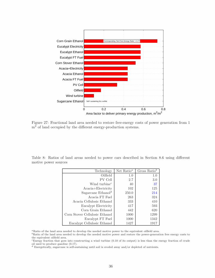
0 0.2 0.4 0.6 0.8

Sugarcane Ethanol

Wind turbine

Oilfield

PV Cell

Acacia FT Fuel

Acacia Ethanol

Acacia+Electricity

Corn Stover Ethanol

Eucalypt FT Fuel

Eucalypt Ethanol


Corn Grain Ethanol Corresponding ’Net Free Energy Ratio’ = 0.77

Self−sustaining for a while

Area factor to deliver primary energy production, m2/m2

Figure 27: Fractional land area needed to restore free-energy costs of power generation from 1m2 of land occupied by the different energy-production systems.

Table 8: Ratios of land areas needed to power cars described in Section 8.6 using differentmotive power sources

Technology Net Ratioa Gross Ratiob

Oilfield 1.0 1.0PV Cell 2.7 3.0

Wind turbinec 40 37Acacia+Electricity 102 125

Sugarcane Ethanold 250.0 214Acacia FT Fuel 263 324

Acacia Cellulosic Ethanol 333 410Eucalypt Electricity 417 593Corn Grain Ethanol 442 620

Corn Stover Cellulosic Ethanol 1000 1299Eucalypt FT Fuel 1000 1342

Eucalypt Cellulosic Ethanol 1427 1917

aRatio of the land area needed to develop the needed motive power to the equivalent oilfield area.bRatio of the land area needed to develop the needed motive power and restore the power-generation free energy costs tothe equivalent oilfield area.cEnergy fraction that goes into constructing a wind turbine (0.10 of its output) is less than the energy fraction of crudeoil used to produce gasoline (0.17).d Energetically, sugarcane is self-sustaining until soil is eroded away and/or depleted of nutrients.

36

0.001 0.01 0.1 1 10

Oilfield

PV Cell

Wind turbine

Acacia+Electricity

Sugarcane Ethanol

Acacia FT Fuel

Acacia Ethanol

Corn Grain Ethanol


Corn Stover Ethanol

Eucalypt FT Fuel

Eucalypt Ethanol

Net Hectares to Drive IC or Electrical Car 15,000 miles

Figure 28: The net area of land needed just to power an efficient (40 mpg) IC engine car or anall-electric car equivalent to 100 mpg, and drive it 15000 miles per year. Note that the plot’sx-axis is logarithmic and the area increases by a factor of 10000 from left to right.

0.001 0.01 0.1 1 10

Oilfield

PV Cell

Wind turbine

Acacia+Electricity

Sugarcane Ethanol

Acacia FT Fuel

Acacia Ethanol


Corn Grain Ethanol

Corn Stover Ethanol

Eucalypt FT Fuel

Eucalypt Ethanol

Gross Hectares to Drive IC or Electrical Car 15,000 miles

Figure 29: The total area of land needed to power an efficient (40 mpg) IC engine car or anall-electric car equivalent to 100 mpg, and drive it 15000 miles per year. Most of the free energycosts of fuels, fertilizers, and some environmental costs of power generation are accounted for.Note that the plot’s x-axis is logarithmic and the area increases by a factor of 10000 from leftto right.

37

9 Conclusions

In this paper I have painted a radical vision of a world in which fossil fuels and agrofuels willbe used increasingly less in transportation vehicles. Gradually, these fuels will be replaced byelectricity stored in the vehicle batteries. With time the batteries will get better, and electricmotors will take over powering the vehicles. The sources of electricity for the batteries willbe increasingly solar photovoltaic cells and wind turbines. The vagaries of cloudy skies andirregular winds will be alleviated to a large degree by the surplus batteries being recharged andshared locally, with no transmission lines out of a neighborhood or city.

I have shown that even mediocre solar cells that cost 1/3 of their life-time electricity produc-tion to be manufactured are at least 100 times more efficient than the current major agrofuelsystems. When deployed these cells will not burn forests; kill living things on land, in the air,and in the oceans; erode soil; contaminate water; and emit astronomic quantities of greenhousegases. Unlike agrofuels, the solar cells will not take away food and environment from the largestpart of the human population in the tropics, and they will not contribute to untold corruption,human misery, squalor, and slave labor. Each hectare of solar cells will replace 70, all the wayup to 650 hectares of fields and tree plantations. This means significant opportunities to storeatmospheric carbon in tree and other plant mass for the next two- or three hundred years.Finally, by the time we will have to replace the early generations of solar cells in 30 to 40 years,many of the current agrofuel systems will be degraded ecological deserts with displaced humanpopulations.

I have also shown you that the Earth simply cannot produce the vast quantities of biomasswe want to use to prolong our unsustainable lifestyles, while slowly committing suicide as aglobal human civilization.

In passing, I have noted that the “cellulosic biomass” refineries are very inefficient, currentlyimpossible to scale, and incapable of ever catching up with the runaway need to feed one billiongasoline- and diesel-powered cars and trucks.

Finally, no future transportation system will allow complete “freedom of personal trans-portation” for everyone. I suggest that good public transportation systems will free many, ifnot most people from personal transportation.

Acknowledgements

I would like to thank the OECD for inviting me and giving an opportunity to speak on theurgent topic of agrofuels.

This work was carefully reviewed and critiqued by Drs. John Benemann, Ignacio

Chapela, John Newman, Ron Steenblik, Dmitriy Silin, and Ron Swanson, as wellas my Ph.D. graduate student, Mr. Greg Croft, and my son Lucas Patzek. I am verygrateful to the reviewers for their valuable suggestions, thoroughness, directness, and dry senseof humor.

The opinions expressed in this paper are those of the author, who is solely responsible forits content and any errors or omissions.

References

Anonymous 2007, Carving up the Congo, Report, Parts I – III, Greenpeace, Washington, DC,www.greenpeace.org/usa/news/rainforest-destruction-in-afri.

Badger, P. C. 2002, Trends in new crops and new uses, Chapt. Ethanol from Cellulose: AGeneral Review, pp 17 – 21, ASHS Press, Alexandria, VA.

Berner, R. A. 2001, Modeling atmospheric o2 over Phanerozoic time, Geochim. Cosmochim.Acta 65: 685 – 694.

38

Berner, R. A. 2003, The long-term carbon cycle, fossil fuels and atmospheric composition,Nature 426: 323 – 326.

Bird, R. B., Stewart, W. E., and Lightfoot, E. N. 1960, Transport phenomena, John Wiley &Sons, New York.

Bossel, U. 2003, Efficiency of Hydrogen Fuel Cell, Diesel-SOFC-Hybrid and Battery ElectricVehicles, Technical report, European Fuel Cell Forum, Morgenacherstrasse 2F, CH-5452Oberrohrdorf, Switzerland, http://www.efcf.com.

Capra, F. 1996, The Web of Life, Anchor Books, A Division of Random House, Inc., NewYork.

Cramer, W. and et al. 1995, Net Primary Productivity – Model Intercomparison Activity,Report 5, IGBP/GAIM, Washington, DC, gaim.unh.edu/Products/Reports/Report−5/-report5.pdf.

Davis, M. 2002, Late Victorian Holocausts: El Nino Famines and the Making of the ThirdWorld, Verso, London.

De Groot, S. R. and Mazur, P. 1962, Non-Equilibrium Thermodynamics, North-Holland,Amsterdam, p. 45.

Domalski, E. S., Jobe Jr., T. L., and Milne, T. A. (eds.) 1987, Thermodynamic Data for BiomassMaterials and Waste Components, The American Society of Mechanical Engineers, UnitedEngineering Center, 345 East 47th Street, New York, N.Y. 10017.

Glansdorff, P. and Prigogine, I. 1971, Thermodynamic Theory of Structure, Stability and Fluc-tuations, John Wiley & Sons, New York, p. 35.

Grimm, K. A. 1998, Phosphorites feed people: Finite fertlizer ores impact Canadian and globalfood security, The Monitor, www.eos.ubc.ca/personal/grimm/phosphorites.html.

Hayden, H. C. 2002, The Solar Fraud: Why Solar Energy Won’t Run the World, Vales LakePublishing Llc., New York.

Heinsch, F. A. and et al. 2003, User’s Guide GPP and NPP (MOD17A2/A3) Products NASAMODIS Land Algorithm, Report, NASA, Washington, DC, www.ntsg.umt.edu/modis/-MOD17UsersGuide.pdf.

Hurtt, G. C., Rosentrater, L., Frolking, S., and Moore, B. 2001, Linking Remote-SensingEstimates of Land Cover and Census Statistics on Land Use to Produce Maps of Land Useof the Conterminous United States, Global Biogeochem. Cycles 15(3): 673 – 685.

Jacques, K. A., Lyons, T. P., and Kelsall, D. R. (eds.) 2003, The Alcohol Textbook, NottinghamUniversity Press, Nottingham, GB, 4 edition.

Khosla, V. 2006, Biofuels: Think outside the Barrel, www.khoslaventures.com/presentations/-Biofuels.Apr2006.ppt, Also see the video version at video.google.com/videoplay?docid=-570288889128950913.

Lee, D.-K., Owens, V. N., Boe, A., and Jeranyama, P. 2007, Composition of HerbaceousBiomass Feedstocks, Report SGINC1-07, Plant Science Department, North Central SunGrant Center, South Dakota State University, Box 2140C, Brookings, SD 57007.

Lovelock, J. 1979, Gaia – A new look at life on the Earth, Oxford University Press, Oxford,GB.

Lovelock, J. 1988, The Ages of Gaia, A Biography of Our Living Earth, W. W. Norton & Co.Inc., New York.

Lugo, A. E. and Brown, S. 1986, Steady state terrestrial ecosystems and the global carboncycle, Vegetatio 68: 83–90.

Mokany, K., Raison, R. J., and Prokushkin, A. S. 2006, Critical analysis of root : shoot ratiosin terrestrial biomes, Global Change Biology 12: 84 – 96.

Montgomery, D. R. 2007, Soil erosion and agricultural sustainability, PNAS 104(33): 13268– 13272.

Napitupulu, M. and Ramu, K. L. V. 1982, Development of the Segara Anakan area of CentralJava, in Proceedings of the Workshop on Coastal Resources Management in the CilacapRegion, pp 66 – 82, Gadjah Mada University, Yogyakarta.

Osborne, J. W. 1970, The Silent Revolution: The Industrial Revolution in England as a Source

39

of Cultural Change, Charles Scribner’s Sons, New York.Page, S. E., Siegert, F., Rieley, J. O., V. Boehm, H.-D., Jaya, A., and Limin, S. 2002, The

amount of carbon released from peat and forest fires in Indonesia during 1997, Nature420(6911): 61 – 65.

Patzek, L. J. and Patzek, T. W. 2007, The Disastrous Local and Global Impacts of TropicalBiofuel Production, Energy Tribune March: 19 – 22.

Patzek, T. W. 2004, Thermodynamics of the corn-ethanol biofuel cycle, Critical Re-views in Plant Sciences 23(6): 519–567, An updated web version is at http://-petroleum.berkeley.edu/papers/patzek/CRPS416-Patzek-Web.pdf.

Patzek, T. W. 2006a, A First-Law Thermodynamic Analysis of the Corn-Ethanol Cycle, NaturalResources Research 15(4): 255 – 270.

Patzek, T. W. 2006b, Letter, Science 312(5781): 1747.Patzek, T. W. 2006c, The Real Biofuels Cycles, Online Supporting Material for Science

Letter, Available at petroleum.berkeley.edu/patzek/BiofuelQA/Materials/RealFuelCycles-Web.pdf.

Patzek, T. W. 2007, Earth, Humans and Energy, CE170 Class Reader, University of Califonia,Berkeley.

Patzek, T. W. and Pimentel, D. 2006, Thermodynamics of energy production frombiomass, Critical Reviews in Plant Sciences 24(5–6): 329–364, Available at http://-petroleum.berkeley.edu/papers/patzek/CRPS-BiomassPaper.pdf.

Perlack, R. D., Wright, L. L., Turhollow, A. F., L., G. R., Stokes, B. J., and Erbach, D. C. 2005,Biomass as feedstock for a bioenergy and bioproducts industry: The technical feasibility of abillion-ton annual supply, Joint Report, Prepared by U.S. Department of Energy, U.S. De-partment of Agriculture, Environmental Sciences Division, Oak Ridge National Laboratory,P.O. Box 2008, Oak Ridge, Tennessee 37831-6285, Managed by: UT-Battelle, LLC for theU.S. Department of Energy under contract DE-AC05-00OR22725 DOE/GO-102005-2135ORNL/TM-2005/66.

Prigogine, I. 1945, Etude thermodynamique des phenomenes irreversibles. These d’agregationpresentee en 1945 a l’Universite Libre de Bruxelles, Acad. Roy. Belg. Bull. Cl. Sc. 31: 600.

Randerson, J. T., Chapin, F. S., Harden, J. W., Neff, J. C., and Harmone, M. E. 2001, Netecosystem production: A comprehensive measure of net carbon accumulation by ecosystems,Ecological Applications 12(4): 2937 – 947.

Reichle, D. E., O’Neill, R. V., and Harris, W. F. 1975, Unifying concepts in ecology, Chapt.Principles of energy and material exchange in ecosystems, pp 27 – 43, Dr. W. Junk B. V.Publishers, The Hague, The Netherlands.

Ricklefs, R. E. (ed.) 1990, Ecology, W. H. Freeman & Company, New York, 3 edition.Ross, J. and Vlad, M. O. 2005, Exact Solutions for the Entropy Production Rate of Several

Irreversible Processes, J. Phys. Chem. A 109: 10607 – 10612.Running, S. W., Thornton, P. E., and et al. 2000, Methods in Ecosystem Science, Chapt. Global

terrestrial gross and net primary productivity from the Earth Observing System, pp 44 –57, Springer Verlag, New York.

Ryan, M. G. 1991, Effects of Climate Change on Plant Respiration, The Ecological Society ofAmerica 1(2): 157–167.

Saha, B. C., Iten, L. B., Cotta, M. A., and Wu, Y. V. 2005, Dilute acid pretreatment, enzymaticsaccharification and fermentation of wheat straw to ethanol, Process Biochemistry 40: 3693– 3700.

Schimel, D. and Baker, D. 2002, The wildfire factor, Nature 420(6911): 29 – 30.Schmidt, A., Zschetzsche, A., and Hantsch-Linhart, W. 1993, Analyse von biogenen Brennstof-

fen, Report, TU Wien, Institut fur Verfahrens-, Brennstoff- und Umwelttechnik, Vienna,Austria, www.vt.tuwien.ac.at/Biobib/fuel98.html.

Smil, V. 1985, Carbon – Nitrogen – Sulfur – Human Interferences in Grand Biospheric Cycles,Plenum Press, New York and London.

Songa, C. and Woodcock, C. E. 2003, A regional forest ecosystem carbon budget model:

40

Impacts of forest age structure and landuse history, Ecological Modelling 164: 33 – 47.Steynberg, A. P. and Nel, H. G. 2004, Clean coal conversion options using Fischer-Tropsch

technology, Fuel 83(6): 765 – 770.Stocking, M. A. 2003, Tropical Soils and Security: The Next 50 years, Science 302(5649):

1356 – 1359.Voet, D. and Voet, J. G. 2004, Biochemistry, John Wiley & Sons, New York, 3 edition, pp.

574 – 579.von Englehardt, W., Goguel, J., Hubbert, M. K., Prentice, J. E., Price, R. A., and Trumpy, R.

1975, Earth Resources, Time, and Man - A Geoscience Perspective, Environmental Geology1: 193 – 206.

Webster 1993, Webster’s Third New International Dictionary of the English Language -Unabridged, Encyclopædia Britannica, Inc., Chicago.

41

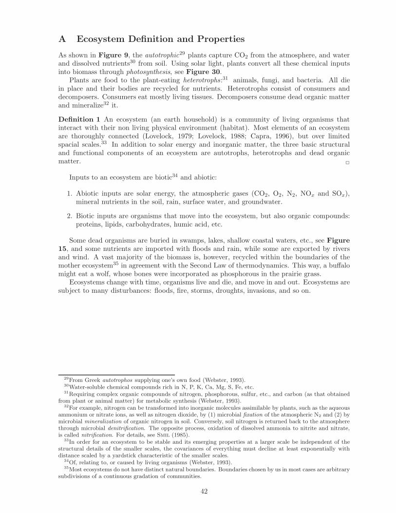
A Ecosystem Definition and Properties

As shown in Figure 9, the autotrophic29 plants capture CO2 from the atmosphere, and waterand dissolved nutrients30 from soil. Using solar light, plants convert all these chemical inputsinto biomass through photosynthesis, see Figure 30.

Plants are food to the plant-eating heterotrophs:31 animals, fungi, and bacteria. All diein place and their bodies are recycled for nutrients. Heterotrophs consist of consumers anddecomposers. Consumers eat mostly living tissues. Decomposers consume dead organic matterand mineralize32 it.

Definition 1 An ecosystem (an earth household) is a community of living organisms thatinteract with their non living physical environment (habitat). Most elements of an ecosystemare thoroughly connected (Lovelock, 1979; Lovelock, 1988; Capra, 1996), but over limitedspacial scales.33 In addition to solar energy and inorganic matter, the three basic structuraland functional components of an ecosystem are autotrophs, heterotrophs and dead organicmatter. 2

Inputs to an ecosystem are biotic34 and abiotic:

1. Abiotic inputs are solar energy, the atmospheric gases (CO2, O2, N2, NOx and SOx),mineral nutrients in the soil, rain, surface water, and groundwater.

2. Biotic inputs are organisms that move into the ecosystem, but also organic compounds:proteins, lipids, carbohydrates, humic acid, etc.

Some dead organisms are buried in swamps, lakes, shallow coastal waters, etc., see Figure15, and some nutrients are imported with floods and rain, while some are exported by riversand wind. A vast majority of the biomass is, however, recycled within the boundaries of themother ecosystem35 in agreement with the Second Law of thermodynamics. This way, a buffalomight eat a wolf, whose bones were incorporated as phosphorous in the prairie grass.

Ecosystems change with time, organisms live and die, and move in and out. Ecosystems aresubject to many disturbances: floods, fire, storms, droughts, invasions, and so on.

29From Greek autotrophos supplying one’s own food (Webster, 1993).30Water-soluble chemical compounds rich in N, P, K, Ca, Mg, S, Fe, etc.31Requiring complex organic compounds of nitrogen, phosphorous, sulfur, etc., and carbon (as that obtained

from plant or animal matter) for metabolic synthesis (Webster, 1993).32For example, nitrogen can be transformed into inorganic molecules assimilable by plants, such as the aqueous

ammonium or nitrate ions, as well as nitrogen dioxide, by (1) microbial fixation of the atmospheric N2 and (2) bymicrobial mineralization of organic nitrogen in soil. Conversely, soil nitrogen is returned back to the atmospherethrough microbial denitrification. The opposite process, oxidation of dissolved ammonia to nitrite and nitrate,is called nitrification. For details, see Smil (1985).

33In order for an ecosystem to be stable and its emerging properties at a larger scale be independent of thestructural details of the smaller scales, the covariances of everything must decline at least exponentially withdistance scaled by a yardstick characteristic of the smaller scales.

34Of, relating to, or caused by living organisms (Webster, 1993).35Most ecosystems do not have distinct natural boundaries. Boundaries chosen by us in most cases are arbitrary

subdivisions of a continuous gradation of communities.

42

Respiration

H2O O2

DarkReactions

CO2Glucose

CO2

LightReactions

NADPH+ATP NADP++ADP+PI

O2 H2O

Sun

Photo

synth

esis

Figure 30: The light reactions use photons to strip protons from water and store energy inNADPH (nicotinamide adenine dinucleotide phosphate) and ATP (adenosine 5′-triphosphatenucleotide). Both these molecules are used to reduce CO2 and combine carbon with hydro-gen and phosphate in the Calvin Cycle or dark reactions: 3 CO2 + 9 ATP + 6 NADPH →

glyceraldehyde-3-phosphate + 9 ADP + 8 PI + 6 NADP+. Here ADP is adenosine diphosphate,PI is inorganic phosphate, and NADP+ is the oxidized form of NADPH. Glyceraldehyde-3-phosphate may be converted to other carbohydrates such as metabolites (fructose-6-phosphateand glucose-1-phosphate), energy stores (sucrose or starch), or cell-wall constituents (celluloseand hemicelluloses). By respiring plants consume O2 and convert their energy stores back toCO2 and water.

43

B Mass Balance of Carbon in an Ecosystem

An eco-system is a system known to thermodynamics only if a three-dimensional surface36 fullyenveloping the system’s contents is imagined for the life-span of the ecosystem. Of course, thissurface may itself be time-dependent, but not right now.

Once there is a boundary, the carbon mass accumulation in the ecosystem is defined throughthe carbon mass flow crossing its boundary, and the interior carbon sources and sinks. Thegeneral mass-balance equation that describes all physical systems, (see, e.g., Bird et al. (1960)),can be written for carbon in the following way:

dC

dt︸︷︷︸

Rate of livingcarbon

accumulation

= −

∮

BoundaryF · ndA

︸︷︷︸

Net rate ofcarbonflow out

+∑

Sources −∑

Sinks︸︷︷︸

Net rate ofcarbon

production inside

kg C s−1 (6)

Here F is the overall carbon flux vector, n is the unit outward normal to the system boundary,and the summation (integral) is over the entire system boundary. The sources inside the systemvolume are the photosynthesizing autotrophs, and the sinks are the respiring autotrophs andheterotrophs, fires, soil carbon oxidation, volatile hydrocarbon production, etc. The overallcarbon flux F is the vector sum of several different mechanisms of carbon mass exchange, suchas convection with air, convection with moving heterotrophs, convection with soil-, river- andflood water, convection with eroded soil, etc. Each of the particular fluxes is nonzero over thoseparts of the system boundary where it operates and zero elsewhere.

Let’s define mi, the overall outward carbon mass flow rate due to a specific flux i; GrossPrimary Production (GPP), the sum of autotroph photosynthesis sources; Ra, the overall au-totroph respiration sink; Rh, the overall heterotroph respiration sink; Rf , the overall fire sink;Rv, the overall volatile hydrocarbon production sink; Rs, the soil carbon oxidation sink; Rb,the carbon burial sink; etc.

mi =

∮

BoundaryFi · ndA

GPP =∑

Sources

R = Ra + Rh + Rf + Rv + Rs + · · · =∑

Sinks

(7)

Then

dC

dt= −

∑

i

mi + GPP − (Ra + Rh)︸︷︷︸

EcosystemRespiration

Re

− (Rf + Rv + Rs . . . )︸︷︷︸

Non respiratorysinks of C

(8)

In order to correspond to the dominant time scale of observations, the “instantaneous” carbon

36A 3D curvilinear box extending above the tallest feature of the ecosystem, and below topsoil, river, lake andstream bottoms, etc.

44

mass balance equation must be further time-averaged, as denoted by the angular brackets:

1

τ2 − τ1

∫ τ2

τ1

dC

dtdt = −

∑

i

1

τ2 − τ1

∫ τ2

τ1

mi(t)dt+

+1

τ2 − τ1

∫ τ2

τ1

GPP(t)dt −1

τ2 − τ1

∫ τ2

τ1

R(t)dt

C(τ2) − C(τ1)

τ2 − τ1=

⟨dC

dt

⟩

= −

∑

i

< mi > + < GPP > − < R >

︸︷︷︸

Net EcosystemProductivity

< NEP >

(9)

Note that in spirit, the last Eq. (9) is similar to Eqs. (1) and (2) in Randerson et al. (2001),which unfortunately do not distinguish between fluxes and sources and sinks.

NEP is defined here as the net carbon accumulation by an ecosystem, just as in Rander-

son et al. (2001). It explicitly incorporates all of the carbon fluxes from an ecosystem, andthe interior sources and sinks, including lateral transfers among ecosystems, autotrophicrespiration, heterotrophic respiration, losses associated with disturbances, dissolved andparticulate carbon losses, carbon burial, and volatile organic compound emissions.

Now, if the time of observation is long enough, the average rate of carbon accumulation ina stable ecosystem should tend to zero because of the Second Law of thermodynamics. Globalcarbon burial has been about 0.1 percent of terrestrial NPP, see Figure 15. Thus, on a timescale of a couple of centuries (Lugo and Brown, 1986; Berner, 2001; Berner, 2003), one maypostulate that the rate of carbon accumulation is minuscule compared with the fluxes, sourcesand sinks, and

< NEP >≈ 0 (10)

Given enough time, stable ecosystems will settle into steady states and recycle almost allcarbon (and all other nutrients) in them, see Table 9.

Soils, landscapes, and plant communities evolve together through an interdependence onthe difference between the rate of soil erosion and soil production (Montgomery, 2007). Atsteady state this difference must be zero on the average., i.e., the soil erosion rate is equal tothe geologic rate of soil production and some equilibrium thickness of soil persists over longtime intervals.

Geological erosion rates generally increase from the gently sloping lowland landscapes (<10−4 to 1 mm/yr), to moderate gradient hillslopes of soil-mantled terrain (0.001 to 1 mm/yr),and steep tectonically active alpine landscapes (0.1 to > 10 mm/yr) (cf. Montgomery (2007)and the references therein).

Rates of soil erosion under conventional agricultural practices almost uniformly exceed 0.029to 0.173 mm/yr (the median and mean geological rate of soil production, respectively), withthe data compiled by Montgomery (2007) exhibiting the median and mean values >1 mm/yr.Erosion rates on the steep mountain slopes in Indonesia easily exceed 30 mm/yr (Napitupuluand Ramu, 1982), and the human-disturbed soil can disappear there within days or months,rather than years.

45

Rates of erosion reported under native vegetation and conventional agriculture show1.3- to >1000-fold increases, with the median and mean ratios of 18- and 124-fold, respec-tively for the studies compiled by Montgomery (2007). From my work on the tropicalplantations (Patzek and Pimentel, 2006) it follows that the respective ratios are even higherin the mechanically-disturbed hilly landscapes.

For this and many other reasons, humanity’s experiment with “Green Revolution” is just alarge but temporary disturbance of natural ecosystems driven by a gigantic multi-decade subsidywith old plant carbon (fossil fuels, fertilizers, and field chemicals) into the vastly simplified, fast-eroding, and – therefore – unstable agricultural systems. As such, these latter systems will nevertest Eq. (10). They will fail much sooner instead.37

In addition, a long time-average of the net carbon flow rate out of the system may also benegligible, as most of it is the CO2 flow rate in for photosynthesis minus the CO2 flow rateout from respiration. The extreme events38, such as fires and floods, will be averaged out andin a stable ecosystem soil erosion should also be low (or the ecosystem would not survive, seeFigure 31). The time-averaged rate of volatile hydrocarbon emissions must be relatively lowtoo, and, therefore, one may postulate that

< GPP > − < R >≈ 0 (11)

When averaged over a sufficiently long time, the gross ecosystem productivity is roughlyequal to the total rate of carbon consumption inside the ecosystem. The origin of thispostulate is also the Second Law of thermodynamics.

37“One alternative,” Prof. Harvey Blanch notes, “is to bioengineer a low-lignin crop that does not requirefertilizer, that doesn’t need much water, and that could be grown on land not suitable for food crops. Theproblem is that lignin is what makes the plant stalks rigid, and without it, a plant would probably be floppyand difficult to harvest. And of course,” he adds, “there might be public resistance to huge plantations of agenetically-modified organism.” Global warming - Building a sustainable biofuel production system, The NewsJournal, College of Chemistry, University of California, Berkeley, 14(1), 2006.

38Disturbances in the ecology parlance.

46

0 500 1000 1500 20000

500

1000

1500

2000

2500

3000

3500

4000

Cro

p yi

eld

kg/h

a−yr

Cumulative soil erosion, tonnes/ha

Phaeozem, ArgentinaFerralsol + Cambisol, BrazilNitosol, KenyaLuvisol + Acrisol, Nigeria

Figure 31: Maize crop yields decay exponentially with eroded soil for a selection of tropicalsoils: Yield = 4000 exp[Cumulative Erosion/r], r = 20 − 300 t ha−1. The initial yield level isset artificially to 4 tonnes of grain needed by one typical household for 1 year in the subhumidtropics. The cumulative erosion of 10 t ha−1

≈ 1 mm of soil loss. So a loss of 2 cm of topsoil inthe tropics is catastrophic. Adapted from Fig. 1 of Stocking (2003).

Table 9: Summary of carbon fluxes in terrestrial ecosystems. Adapted from Tables 1 and 2 in(Randerson et al., 2001) and NASA MODIS data in Table 2

Concept Acronym Global flux Definition

symbol

Gross primary production GPP 110 Gt C/yr a

Autotrophic respiration Ra ∼1/2 of GPP b

Net primary production NPP ∼1/2 of GPP GPP - Ra

Heterotrophic respiration (on land) Rh 82 - 95% of NPP c

Ecosystem respiration Re 91 - 97% of GPP Ra + Rh

Non-CO2 losses Rv + Rs 2.8 - 4.9 Gt C/yr d

Non-respiratory CO2 losses (fire) Rf 1.6 - 4.2 Gt C/yr e

Net ecosystem production NEP 0 ± 2.0 Gt C/yr f

a Carbon uptake by plants during photosynthesis, see Table 2.bRespiratory (CO2) loss by plants for construction, maintenance, or ion uptake, see Table 2.cRespiratory (CO2) loss by the heterotrophic community (herbivores, microbes, etc.).dCO, CH4, isoprene (2-methylbuta-1,3-diene), dissolved inorganic and organic carbon, erosion, etc.These losses are 2.6 to 4.5 % of GPP.eAverage combustion flux of CO2 is 1.5 to 3.8 % of GPP Extreme events, such as the 1997 – 98 El Ninofirestorms in Indonesia are excluded.fTotal carbon accumulation within the ecosystem: GPP - Re − Rf − Rv − Rs − . . . . All human cropsexport about 1.2 to 1.5 Gt C/yr from agricultural ecosystems, while crop residues contain another 1.3 to1.5 Gt C/yr.

47

C Environmental Controls on Net Primary Productivity

Net primary productivity is equal to the product of the rate of photosynthesis per unit leaf areaand the total surface area of the active leaves per unit area of land, minus the rate of plantrespiration per unit area of land. Given sufficient plant nutrients and substrates, temperatureand moisture control the rate of photosynthesis.

Extremely cold and hot temperatures limit the rate of photosynthesis. Within the range oftemperatures that are tolerated, the rate of photosynthesis generally rises with temperature.Most biological metabolic activity takes place between 0 and 50 0C. The optimal temperaturesfor plant productivity coincide with the 15 to 25 0C optimum temperature range of photosyn-thesis.

A growing season is the period when temperatures are sufficiently warm to support photo-synthesis and a positive net primary production. Warmer temperatures support both higherrates of photosynthesis and a longer growing season, resulting in a higher net primary produc-tion – if there are sufficient water and nutrients. The amount of water available to the plant willtherefore limit both the rate of photosynthesis and the area of leaves that can be supported.

The influence of temperature and water availability is interrelated. It is the combinationof warm temperatures and water supply adequate to meet the demands of transpiration thatresults in the highest values of primary productivity. Net primary production in ecosystemsvaries widely, cf. Figure 7 in Cramer et al. (1995) and Table 10:

1. The most productive terrestrial ecosystems are tropical evergreen rainforests with highrainfall and warm temperatures. Their net primary productivity ranges from 700 to 1400g C m−2 yr−1.

2. Temperate mixed forests produce between 400 and 1000 g C m−2 yr−1.

3. Temperate grassland productivity is between 200 and 500 g C m−2 yr−1.

4. Arctic and alpine tundra have productivities of 0 to 300 g C m−2 yr−1.

5. Productivity of the open sea is generally low, 10 to 50 g C m−2 yr−1.

6. Given equal nutrient supplies, productivity in the open waters of the cool temperateoceans tends to be higher than that of the tropical waters.

7. In areas of upwelling, as near the tropical coast of Peru, productivity can exceed 500 gC m−2 yr−1.

8. Coastal ecosystems and continental shelves have higher productivity than open ocean.

9. Swamps and marshes have a net primary production of 1100 g C m−2 yr−1 or higher.

10. Estuaries and coral reefs have a net primary productivity of 900 g C m−2 yr−1. This iscaused by the inputs of nutrients from rivers and tides in estuaries, and the changing tidesin coral reefs.

High primary productivity results from an energy subsidy to the (generally small) ecosystem.This subsidy results from a warmer temperature, greater rainfall, circulating or moving waterthat carries in food or additional nutrients. In the case of agriculture, the subsidy comes fromfossil fuels for cultivation and irrigation, fertilizers, and the control of pests. Sugarcane has anet productivity of 1700 to 2500 g m−2 yr−1 of dry stems, and hybrid corn in the US 800 - 1000g m−2 yr−1 of dry grain.

48

Table 10: Average net primary productivity of ecosystems

Ecosystem Valuea Valueb

g C m−2 yr−1 g m−2 yr−1

Swamp and marsh 1130 2500

Algal bed and reef 900 2000

Tropical forest 830 1800

Estuary 810 1800

Temperate forest 560 1250

Boreal forest 360 800

Savanna 320 700

Cultivated land 290 650

Woodland and shrubland 270 600

Grassland 230 500

Lake and stream 230 500

Continental shelf 160 360

Tundra and alpine meadow 65 140

Open ocean 57 125

Desert scrub 32 70

Rock, ice, and sand 15 –

a www.vendian.org/envelope/TemporaryURL/draft-npp.htmlb (Ricklefs, 1990). Note that Column 2 is ∼Column 1 × 2.2, corresponding to the mean molecular weight

of dry biomass of 26 g/mol per 1 carbon atom, a little less than 27 g/mol in glucose starch, CH2O –

1/6H2O. A typical molecular composition of dry woody biomass is CH1.4O0.6, MW = 23 g/mol.

49

Documents

How Can We Outlive Our Way of Life? - OECD...How Can We Outlive Our Way of Life? Tad W. Patzek Department of Civil and Environmental Engineering The University of California Berkeley,