How Are SNAP Benefits Spent?Evidence from a Retail Panel

Justine Hastings Jesse M. Shapiro∗

Brown University and NBER

March 2018

Abstract

We use a novel retail panel with detailed transaction records to study the effect of the Supple-mental Nutrition Assistance Program (SNAP) on household spending. We use administrativedata to motivate three approaches to causal inference. The marginal propensity to consumeSNAP-eligible food (MPCF) out of SNAP benefits is 0.5 to 0.6. The MPCF out of cash ismuch smaller. These patterns obtain even for households for whom SNAP benefits are eco-nomically equivalent to cash because their benefits are below their food spending. Using asemiparametric framework, we reject the hypothesis that households respect the fungibility ofmoney. A model with mental accounting can match the facts.

Keywords: in-kind transfers, mental accounting, fungibilityJEL: D12, H31, I38

∗This work has been supported (in part) by awards from the Laura and John Arnold Foundation, the Smith Richard-son Foundation, the National Science Foundation under Grant No. 1658037, the Robert Wood Johnson Foundation’sPolicies for Action program, and the Russell Sage Foundation. Any opinions expressed are those of the author(s)alone and should not be construed as representing the opinions of these Foundations. We also appreciate support fromthe Population Studies and Training Center at Brown University. This project benefited from the suggestions of KenChay, Raj Chetty, David Cutler, Amy Finkelstein, John Friedman, Roland Fryer, Xavier Gabaix, Peter Ganong, EdGlaeser, Nathan Hendren, Hilary Hoynes, Larry Katz, David Laibson, Kevin Murphy, Mandy Pallais, Devin Pope,Matthew Rabin, Diane Whitmore Schanzenbach, Andrei Shleifer, Erik Snowberg, and Anthony Zhang, from audi-ence comments at Brown University, Clark University, Harvard University, the Massachusetts Institute of Technology,UC Berkeley, Stanford University, Princeton University, the University of Chicago, Northwestern University, UC SanDiego, New York University, Columbia University, the Vancouver School of Economics, the University of SouthernCalifornia, UT Austin, the Quantitative Marketing and Economics Conference, NBER Summer Institute, and fromcomments by discussant J.P. Dubé. We thank our dedicated research assistants for their contributions. E-mail: jus-tine_hastings@brown.edu, jesse_shapiro_1@brown.edu.

1

1 Introduction

This paper studies how the Supplemental Nutrition Assistance Program (SNAP) affects household

spending. SNAP, the successor to the Food Stamp Program, provides recipient households with a

monthly electronic benefit that can only be spent on groceries. It is the second-largest means-tested

program in the United States after Medicaid (Congressional Budget Office 2013), enrolling 19.6

percent of households in the average month of fiscal 2014.1

The program’s design reflects its stated goal of increasing recipient households’ food pur-

chases.2 Yet for the large majority of recipient households who spend more on food than they

receive in benefits,3 SNAP benefits are economically equivalent to cash.4 Recent estimates of low-

income US households’ marginal propensity to consume food (MPCF) out of cash income are at

or below 0.1.5 Thus, if households obey traditional demand theory, the program mainly increases

nonfood spending.

This tension between program rhetoric and traditional economic theory matters both for evalu-

ating SNAP and for the basic science of household decision-making. The fungibility of money is a

fundamental prediction of traditional demand theory. It is challenged by the hypothesis of mental

accounting (Thaler 1999), which posits that households treat different sources of income differ-

ently. If households treat SNAP benefits differently from cash, this would likely have important

implications for the modeling of household behavior in this and other contexts.

1Over the months of fiscal 2014, the number of participating households ranged from 22,580,029 to 23,053,620,with an average of 22,744,054 (FNS 2016a). There were 116,211,092 households in the US on average from 2010-2014 (US Census Bureau 2016).

2On signing the bill to implement the Food Stamp Program, President Lyndon Johnson declared that the programwould “enable low-income families to increase their food expenditures” (Johnson 1964). The Food and NutritionService of the USDA says that SNAP is important for “helping families put food on the table” (FNS 2012).

3Hoynes et al. (2015) find that spending on food at home is at or above the SNAP benefit level for 84 percent ofSNAP recipient households. Trippe and Ewell (2007) report that 73 to 78 percent of SNAP recipients spend at least10 percent more on food than they receive in SNAP benefits.

4To fix ideas, consider a household with monthly income y and SNAP benefits b. If the household spendsf on SNAP-eligible food then it has y−max(0, f −b) available to buy other goods. Let U ( f ,n) denote thehousehold’s strictly monotone, differentiable, and strictly quasiconcave utility function defined over the dollaramount of SNAP-eligible food consumption f and other consumption n. Suppose that there is a solution f ∗ =argmax f U ( f ,y−max(0, f −b)) such that f ∗ > b. The first-order necessary condition for this program is a nec-essary and sufficient condition for a solution to the program max f U ( f ,y+b− f ) in which the benefits are given incash. Therefore f ∗ = argmax f U ( f ,y+b− f ). See Mankiw (2000) and Browning and Zupan (2004) for a textbooktreatment.

5Castner and Mabli (2010) estimate an MPCF out of cash income of 0.07 for SNAP participants. Hoynes andSchanzenbach (2009) estimate an MPCF out of cash income of 0.09-0.10 for populations with a high likelihood ofparticipating in the Food Stamp Program.

2

In this paper, we analyze a novel panel consisting of detailed transaction records from February

2006 to December 2012 for nearly half a million regular customers of a large US grocery retailer.

The data contain information on method of payment, allowing us to infer SNAP participation.

We use three approaches to estimating the causal effect of SNAP on household spending: a

panel event-study design using trends prior to SNAP adoption to diagnose confounds, an instru-

mental variables design exploiting plausibly exogenous variation in the timing of program exit,

and a differences-in-differences design exploiting legislated changes to benefit schedules.

We motivate these three approaches with findings from administrative data. Rhode Island ad-

ministrative data show that household circumstances change fairly smoothly around SNAP en-

rollment, motivating our panel event-study design. The administrative data also confirm our ex-

pectation that SNAP spell lengths are often divisible by six months because of the recertification

process (Klerman and Danielson 2011; Mills et al. 2014; Scherpf and Cerf 2016), motivating

our instrumental-variables design. National administrative records show discrete jumps in SNAP

benefits associated with legislated program changes in 2008 and 2009, motivating our differences-

in-differences design.

Panel event-study plots show that after adoption of SNAP, households in the retailer panel

increase SNAP-eligible spending by about $110 a month, equivalent to more than half of their

monthly SNAP benefit, thus implying an MPCF out of SNAP between 0.5 and 0.6. Plots motivated

by our instrumental-variables and differences-in-differences designs also imply an MPCF out of

SNAP in the range of 0.5 to 0.6. By contrast, we estimate small effects of SNAP on nonfood

spending.

We exploit large swings in gasoline prices during our sample period to estimate the MPCF

out of cash for the SNAP-recipient households in the retail panel, in a manner similar to Gelman

et al. (2017). Data on retail panelists’ gasoline purchases show that increases in gasoline prices

lead to significant additional out-of-pocket fuel expenses for SNAP-recipient households, but little

change in SNAP-eligible spending. We estimate a very low MPCF out of changes in fuel spending,

consistent with other estimates of the MPCF out of cash for low-income populations.

Our findings indicate that the MPCF out of SNAP is greater than the MPCF out of other income

sources. We show that this pattern holds even for households for whom SNAP benefits should be

fungible with cash because their SNAP-eligible spending before SNAP receipt exceeds their SNAP

3

benefits.

In our analysis, we consider several possible challenges to the internal and external validity

of the estimated MPCF out of SNAP. These challenges follow from the fact that our retail panel

includes only purchases by regular customers at a single retail chain.

The first challenge is that we may mismeasure transitions on to and off of SNAP, which we infer

using data on mode of payment at the retailer. We use data on the universe of SNAP transactions

in Rhode Island to develop and validate our approach to measuring program transitions.

The second challenge is that SNAP participation may impact households’ choice of retailer,

which would affect the conclusions from our first two research designs. Nationally representative

survey data, and data from the Nielsen Homescan Consumer Panel, show that SNAP participation

is only weakly related to a household’s choice of retailer. We perform simulations to quantify the

sensitivity of our estimates to assumptions about the relationship between SNAP participation and

choice of retailer.

The third challenge is that household circumstances change in the period surrounding entry

into the program, and we know relatively little about the households in the retail panel beyond their

purchases. This challenge is especially important for our first research design. We argue that trends

in food spending prior to adoption suggest a small role for confounding changes in circumstances,

and use the instrumental variables approach proposed in Freyaldenhoven et al. (2018) to account

directly for such confounds.

The fourth challenge is that our retail panel is not a nationally representative random sample,

which limits the external validity of our estimates. We compare several features of our panel to

nationally and locally representative statistics to gauge differences in the populations.

After laying out our evidence on the MPCF, we develop an economic model of monthly food

spending by households for whom SNAP benefits are economically equivalent to cash. We show

how to test the hypothesis of fungibility, allowing for the endogeneity of cash income and SNAP

benefits, and for the possibility that different households’ consumption functions do not share a

common parametric structure. Our tests consistently reject the null hypothesis that households

treat SNAP benefits as fungible with other income.

We turn next to the possible psychological reasons for departures from fungibility. We discuss

responses to qualitative interviews conducted at a food pantry as part of a Rhode Island state pilot

4

proposal to modify SNAP benefit timing. Interviewees often express different intentions when

asked how they would spend additional SNAP benefits or additional cash. Using our retail panel,

we show that SNAP receipt reduces shopping effort, measured as either the store-brand share of

expenditures or the share of purchases on which coupons are redeemed, but only for SNAP-eligible

items.

Motivated by these findings, we specify a parametric model of behavior in which households

choose expenditures and shopping effort subject to short-run time preference (Laibson 1997) and

mental accounting (Thaler 1999). Following Farhi and Gabaix (2015), we operationalize mental

accounting as a linear cost of deviating from a default level of food spending that moves one-for-

one with SNAP benefits. We fit some model parameters to our data and choose others based on

past research. Short-run time preference alone cannot explain the observed MPCF because SNAP

benefits are too small relative to desired food spending to constrain household spending even at

the beginning of the month. Introducing mental accounting allows the fitted model to match the

observed MPCF out of SNAP and the key qualitative patterns in shopping effort. The fitted model

implies that a household would be willing to give up 0.84 percent (0.0084 log points) of monthly

consumption to avoid the psychological cost of a $100 deviation from default spending.

This paper contributes to a large literature on the effects of SNAP, and its predecessor the Food

Stamp Program, on food spending, recently reviewed by Bitler (2015) and Hoynes and Schanzen-

bach (2016). There are four strands to this literature. The first strand studies the effect of converting

food stamp benefits to cash.6 The second strand, reviewed in Fox et al. (2004), either compares

participants to nonparticipants or relates a household’s food spending to its benefit amount in the

cross-section or over time.7 The third strand studies randomized evaluations of program extensions

or additions.8

6Moffitt (1989) finds that a cashout in Puerto Rico did not affect food spending. Wilde and Ranney (1996) findthat behavior in two randomized cashout interventions is not consistent with fungibility; Schanzenbach (2002) findsthat behavior in these same interventions is consistent with fungibility. Fox et al. (2004) question the validity ofthe findings from Puerto Rico and one of the randomized interventions, arguing that the best evidence indicates thatcashout reduces food spending.

7Wilde (2001) and Hoynes and Schanzenbach (2009), among others, criticize this strand of the literature for usinga source of variation in program benefits that is likely related to non-program determinants of spending. Wilde et al.(2009) address the endogeneity of program benefits by exploiting variation in whether household food spending isconstrained by program rules. Li et al. (2014) use panel data to study the evolution of child food insecurity in themonths before and after family entry into the food stamp program.

8Collins et al. (2016) study a randomized evaluation of the Summer Electronic Benefit Transfer for Childrenprogram and use survey data to estimate an MPCF out of program benefits of 0.58.

5

The fourth strand exploits policy variation in program availability and generosity. Studying the

initial rollout of the Food Stamp Program using survey data, Hoynes and Schanzenbach (2009)

estimate an MPCF out of food stamps of 0.16 to 0.32, with confidence interval radius ranging from

0.17 to 0.27. Hoynes and Schanzenbach (2009) estimate an MPCF out of cash income of 0.09 to

0.10 and cannot reject the hypothesis that the MPCF out of food stamps is equal to the MPCF out

of cash income. Studying the effect of legislated benefit increases between 2007 and 2010 survey

data, Beatty and Tuttle (2015) estimate an MPCF out of SNAP benefits of 0.53 to 0.64 (they do not

report a confidence interval on these values) and an MPCF out of cash income of 0.15.9 Closest to

our study, Bruich (2014) uses retail scanner data with method-of-payment information to study the

effect of a 2013 SNAP benefit reduction, estimating an MPCF out of SNAP benefits of 0.3 with

confidence interval radius of 0.15.10 We estimate an MPCF out of SNAP benefits of 0.5 to 0.6 with

confidence interval radius as low as 0.015, and an MPCF out of cash income of no more than 0.1.

This paper contributes new evidence of violations of fungibility in a large-stakes real-world

decision with significant policy relevance. That households mentally or even physically separate

different income sources according to spending intentions is well-documented in hypothetical-

choice scenarios (e.g., Heath and Soll 1996; Thaler 1999) and ethnographic studies (e.g., Rainwater

et al. 1959). Much of the recent evidence from real-world markets is confined to settings with little

direct policy relevance (e.g., Milkman and Beshears 2009; Hastings and Shapiro 2013; Abeler and

Marklein 2017). Important exceptions include Kooreman’s (2000) study of a child tax credit in

the Netherlands, Jacoby’s (2002) study of a school nutrition program in the Philippines, Feldman’s

(2010) study of a change in US federal income tax withholding, Card and Ransom’s (2011) and

Kooreman et al.’s (2013) studies of employee savings programs in the US and the Netherlands,

respectively, Beatty et al.’s (2014) study of a labeled cash transfer in the UK, and Benhassine et

al.’s (2015) study of a labeled cash transfer in Morocco.11

9Studying the effect of the benefit increase arising from the 2009 American Recovery and Reinvestment Act(ARRA) using survey data, Tuttle (2016) estimates an MPCF out of SNAP of 0.53 with confidence interval radius of0.38. Nord and Prell (2011) estimate the effect of the 2009 benefit expansion on food security and food expenditures.Ratcliffe et al. (2011) and Yen et al. (2008) estimate the effect of SNAP and food stamps, respectively, on foodinsecurity, using state-level policy variables as excluded instruments.

10Bruich (2014) does not report an MPCF out of cash income. Andreyeva et al. (2012) and Garasky et al. (2016)use retail scanner data to describe the food purchases of SNAP recipients, but not to estimate the causal effect of SNAPon spending.

11See also Islam and Hoddinott (2009), Afridi (2010), Shi (2012), and Aker (2017). A closely related literature on“flypaper effects” studies violations of fungibility by governments (Hines and Thaler 1995; Inman 2008).

6

This paper also shows how to test for the fungibility of money without assuming that the con-

sumption function is linear or that the consumption function is identical for all households. Our

approach nests Kooreman’s (2000), but, like Kooreman et al.’s (2013), avoids the concern that a

rejection of fungibility is due to misspecification of functional forms (Ketcham et al. 2016).

Our use of a parametric model to quantify the predictions of multiple psychological departures

from the neoclassical benchmark is similar in spirit to DellaVigna et al. (2017). Hastings and

Shapiro (2013), Ganong and Noel (2017), and Thakral and Tô (2017) also compare the predictions

of alternative psychological models. The only other paper we are aware of that reports an estimate

of a structural parameter of a model of mental accounting based on non-laboratory evidence is

Farhi and Gabaix (2017), who calibrate parameters of their model to match our empirical findings.

In this sense, our paper contributes to the growing literature on structural behavioral economics

(DellaVigna 2017).

2 Motivating evidence from administrative and survey data

2.1 Rhode Island administrative data

We use Rhode Island state administrative records housed in a secure facility at the Rhode Is-

land Innovative Policy Lab (RIIPL) at Brown University. Personally identifiable information has

been removed from the data and replaced with anonymous identifiers that make it possible for

researchers with approved access to join and analyze records associated with the same individual

while preserving anonymity. These records are not linked to our retail panel.

The data include anonymized state SNAP records from October 2004 through June 2016, which

indicate the months of benefit receipt and the collection of individuals associated with each house-

hold on SNAP in each month. We define a SNAP spell to be a contiguous period of benefit receipt.

We assume that an individual belongs to the household of her most recent spell, does not change

households between the end of any given spell and the start of the next spell, and belongs to the

household of her first spell as of the start of the sample period. We determine each individual’s

age in each month, and we exclude from our analysis any household whose membership we can-

7

not uniquely identify in every month,12 or whose adult (over 18) composition changes during the

sample period. The final sample consists of 184,308 unique households. For each household and

month, we compute the total number of children under five years old.

The data also include anonymized administrative records of the state’s unemployment insur-

ance system joined via anonymized identifiers to the individuals in the SNAP records over the same

period. We compute, for each household and quarter,13 the sum of total unemployment insurance

benefits received from and total earnings reported for all individuals who are in the household as

of the quarter’s end.14 We will sometimes refer to this total as “in-state earnings” for short, and we

note that it excludes income sources such as social security benefits and out-of-state earnings.

Finally, the data include anonymized administrative records of all debits and credits to the

SNAP Electronic Benefit Transfer (EBT) cards of Rhode Island residents for the period September

2012 through October 2015. From these we identify all household-months in which the household

received a SNAP benefit and all household-months in which the household spent SNAP benefits at

a large, anonymous retailer in Rhode Island (“Rhode Island Retailer”) chosen to be similar to the

retailer that provided our retail panel.

2.2 Changes in household circumstances around SNAP adoption

Because SNAP is a means-tested program and its eligibility rules incorporate a poverty line stan-

dard, household income and household size are major determinants of SNAP eligibility (FNS

2016b). We therefore hypothesize that entry into SNAP is associated with a decrease in in-state

earnings and an increase in the number of children. Figure 1 shows panel event-study plots of in-

state earnings and number of children as a function of time relative to SNAP adoption, which we

define to occur in the first quarter or month, respectively, of a household’s first SNAP spell. In the

12This can occur either because we lack a unique identifier for an individual in the household or because a givenindividual is associated with multiple households in the same month.

13The quarterly level is the most granular at which earnings data are available. We use data only on household-quarters in which the household is observed for all three months of the quarter. Data on earnings are missing from ourdatabase for the fourth quarter of 2004 and the second quarter of 2011.

14We exclude from our analysis any household-quarter in which the household’s total quarterly earnings exceedthe 99.9999th percentile or in which unemployment insurance benefits in any month of the quarter exceed three timesthe four-week equivalent of the 2016 maximum individual weekly benefit of $707 (Rhode Island Department of Laborand Training 2016).

8

period of SNAP adoption, in-state earnings decline and the number of children rises, on average.15

Past research shows that greater household size and lower household income are associated,

respectively, with greater and lower at-home food expenditures among the SNAP-recipient popu-

lation (Castner and Mabli 2010).16 It is therefore unclear whether these contextual factors should

contribute a net rise or fall in food expenditures in the period of SNAP adoption. Because figure 1

shows that these factors trend substantially in the periods preceding SNAP adoption, we can assess

their net effect by studying trends in spending prior to adoption.

Figure 1 therefore motivates our panel event-study research design, in which we look for sharp

changes in spending around SNAP enrollment, and use trends in spending prior to SNAP adoption

to diagnose the direction and plausible magnitude of confounds.

2.3 Length of SNAP spells and the certification process

When a state agency determines that a household is eligible for SNAP, the agency sets a certi-

fication period at the end of which benefits will terminate if the household has not documented

continued eligibility.17 The certification period may not exceed 24 months for households whose

adult members are elderly or disabled, and may not exceed 12 months otherwise (FNS 2014). In

practice, households are frequently certified for exactly these lengths of time, or for other lengths

divisible by 6 months (Mills et al. 2014).

Figure 2 shows the distribution of SNAP spell lengths in Rhode Island administrative data. The

figure shows clear spikes in the density at spell lengths divisible by 6 months. The online appendix

reports that the change in in-state earnings is economically similar between quarters that do and do

15An analogous plot in the online appendix shows that in-state earnings rise in the quarters leading up to programexit. The online appendix also includes a plot of trends in income and number of children around SNAP adoptionconstructed from the Survey of Income and Program Participation.

16Past research also finds that unemployment—a likely cause of the decline in income associated with SNAPadoption—is associated with a small decline in at-home food expenditure. Using cross-sectional variation in theContinuing Survey of Food Intake by Individuals, Aguiar and Hurst (2005) estimate that unemployment is associatedwith 9 percent lower at-home food expenditure. Using pseudo-panel variation in the Family Expenditure Survey, Bankset al. (1998) estimate that unemployment is associated with a 7.6 percent decline in the sum of food consumed in thehome and domestic energy. Using panel variation in the Panel Study of Income Dynamics, Gough (2013) estimatesthat unemployment is associated with a statistically insignificant 1 to 4 percent decline in at-home food expenditure.Using panel variation in checking account records, Ganong and Noel (2016) estimate that the onset of unemploymentis associated with a 3.1 percent decline in at-home food expenditure.

17Federal rules state that “the household’s certification period must not exceed the period of time during which thehousehold’s circumstances (e.g., income, household composition, and residency) are expected to remain stable” (FNS2014).

9

not contain a spell month divisible by 6.

Figure 2 motivates our instrumental variables research design, which exploits the six-month

divisibility of certification periods as a source of plausibly exogenous timing of program exit.

2.4 Legislated changes in SNAP benefit schedules

The online appendix shows the average monthly SNAP benefit per US household from Febru-

ary 2006 to December 2012, which coincides with the time frame of our retail panel. The series

exhibits two large discrete jumps, which correspond to two legislated changes in the benefit sched-

ule: an increase before October 2008 due to the 2008 Farm Bill, and an increase in April 2009

due to the American Recovery and Reinvestment Act.18 These facts motivate our differences-in-

differences research design, which exploits these legislated benefit increases to estimate the MPCF

out of SNAP.

2.5 Inferring SNAP adoption from single-retailer data

Households can spend SNAP at any authorized retailer (FNS 2012). Because we will conduct our

analysis of household spending using data from a single retail chain, we are at risk of mistaking

changes in a household’s choice of retailer for program entry or exit. We use Rhode Island EBT

records to determine how best to infer program transitions in single-retailer data.

For each K ∈ 1, ...,12 and for each household in the EBT records, we identify all cases

of K consecutive months without SNAP spending at the Rhode Island Retailer followed by K

consecutive months with SNAP spending at the Rhode Island Retailer. We then compute the share

of these transition periods in which the household newly enrolled in SNAP within two months of

the start of SNAP spending at the retailer, where we define new enrollment as receipt of at least

$10 in SNAP benefits following a period of at least three consecutive months with no benefit.

Figure 3 plots the share of households newly enrolling in SNAP as a function of the radius

K of the transition period. For low values of K, many transitions reflect retailer-switching rather

than new enrollments in SNAP. The fraction of transitions that represent new enrollments increases

18Two smaller jumps, in October of 2006 and 2007, coincide with the annual cost of living adjustments to SNAPpayments (FNS 2017b). We do not exploit these smaller changes in our analysis as we expect more precise inferencefrom larger changes in benefits.

10

with K. For K = 6, the fraction constituting new enrollments is 87 percent. When we focus on

households who do the majority of their SNAP spending at the retailer in question—a sample

arguably more comparable to the regular customers in our retail panel—this fraction rises to 96

percent.

Motivated by figure 3, our main analysis of SNAP adoption in the retailer data will use transi-

tions with K = 6 and above, and we will present sensitivity analysis using larger minimum values

of K.

2.6 SNAP participation and choice of retailer

Even if we isolate suitably exogenous changes in SNAP participation and benefits, our analysis of

single-retailer data could be misleading if SNAP participation directly affects retailer choice.

Ver Ploeg et al. (2015) study the types of stores at which SNAP recipients shop using nationally

representative survey data collected from April 2012 through January 2013. For 46 percent of

SNAP recipients, the primary grocery retailer is a supercenter, for 43 percent it is a supermarket,

for 3 percent it is another kind of store, and for 8 percent it is unknown.19 The corresponding

values for all US households are 45 percent, 44 percent, 4 percent, and 7 percent. As with primary

stores, the distribution of alternate store types is nearly identical between SNAP recipients and the

population as a whole. SNAP recipients’ choice of store type is also nearly identical to that of

low-income non-recipients.

The online appendix presents analogous evidence on choice of retail chain using the same data

as Ver Ploeg et al. (2015). We find that SNAP participation is not strongly related to households’

choice of retail chain.

Appendix A and appendix table 1 present the results of a longitudinal analysis of the relation-

ship between SNAP participation and choice of retailer using data from the Nielsen Homescan

Consumer Panel. For the full sample of households, we find that SNAP participation is associated

with a statistically insignificant increase of 0.4 percentage points (or 0.7 percent of the mean) in the

share of spending devoted to the primary retailer. For households whose primary retailer is a gro-

cery store, we find a statistically significant increase of 1.1 percentage points (2.2 percent). Section

19Administrative data show that 84 percent of SNAP benefits are redeemed at supercenters or supermarkets (Castnerand Henke 2011).

11

4.4 shows that our main conclusions are not sensitive to allowing for these estimated changes in

retail choice.

3 Retailer data and definitions

3.1 Household purchases and characteristics

We obtained anonymized transaction-level data from a large U.S. grocery retailer with gasoline sta-

tions on site. The data comprise all purchases in five states made using loyalty cards by customers

who shop at one of the retailer’s stores at least every other month.20 We refer to these customers

as households.

The loyalty card is used to deliver and track promotions (Holmes 2011). Communication

with the retailer indicates that at least 90 percent of purchases involve the use of a loyalty card,

consistent with the magnitude reported by Andreyeva et al. (2013), who also conduct research

using loyalty-card data from a grocery retailer.

We observe 6.02 billion purchases made on 608 million purchase occasions by 486,570 house-

holds from February 2006 through December 2012. We exclude from our analysis the 1,214

households who spend more than $5,000 in a single month.

For each household, the retailer provided us with characteristics including the age and gender of

adult household members, the median years of schooling of adult household members, an indicator

for the presence of children, a categorical measure of household income, and ZIP code. These

are based on a combination of sources, including information supplied by the household when

obtaining the loyalty card, information purchased from third parties, and information imputed

from Census statistics for the local area. We use these data in robustness checks and to explore

heterogeneity in our estimates. We match ZIP codes to counties and states using federal data

files.21

20The retailer also provided us with data on the universe of transactions at a single one of the retailer’s stores. In theonline appendix we show that our estimates of the MPCF are similar between our baseline panel and this alternativepanel.

21We assign ZIP codes to counties and states using the crosswalk for the first quarter of 2010 fromUS Department of Housing and Urban Development (2017). We assign each ZIP code to the county thatcontains the largest fraction of the ZIP code’s residential population, breaking ties at random.

12

For each item purchased, we observe the quantity, the pre-tax amount paid, a flag for the use

of WIC, and the dollar amount of coupons or other discounts applied to the purchase.

For each purchase occasion, we observe the date, a store identifier, and a classification of the

store into a retailer division, which is a grouping based on the store’s brand and distribution geogra-

phy. We also observe a classification of the main payment method used for the purchase, defined as

the payment method accounting for the greatest share of expenditure. The main payment method

categories include cash, check, credit, debit, and a government benefit category that consists of

SNAP, WIC, cash benefits (e.g., TANF) delivered by EBT card, and a number of other, smaller

government programs.

For purchase occasions in March 2009 and later, we further observe the exact breakdown of

spending according to a more detailed classification that itemizes specific government programs.

These data indicate that, excluding WIC transactions, SNAP accounts for 99.3 percent of expendi-

tures classified as a government benefit.

We classify a purchase occasion as a SNAP purchase occasion if the main payment method is a

government benefit and WIC is not used. Using the detailed payment data for purchase occasions

in March 2009 and later, we calculate that SNAP is used in only 0.23 percent of the purchase

occasions that we do not classify as SNAP purchase occasions. Appendix table 2 shows that our

key results are not sensitive to excluding from the sample any household that ever uses WIC.

We define a SNAP month as any household-month with positive total spending across SNAP

purchase occasions.22 Of the household-months in our panel, 7.7 percent are SNAP months. Of

the households in our panel, 42.9 percent experience at least one SNAP month, and 21.6 percent

experience at least two consecutive SNAP months.23

SNAP penetration is lower in the retail panel than in the US as a whole. Calculations in the

online appendix show that an average of 14.5 percent of US households were on SNAP during the

months of the retail sample period. The fraction of households on SNAP is similar when focusing

only on the counties of residence of the households in the retail panel. A possible explanation is

22Using our detailed payment data for March 2009 and later, we can alternatively define a SNAP month as anymonth in which a household uses SNAP. This definition agrees with our principal definition in all but 0.27 percent ofhousehold-months.

23Calculations in the online appendix show that in the 2008 Survey of Income and Program Participation, house-holds are on SNAP in 9.0 to 11.9 percent of survey months, and 17.2 to 21.7 percent of households are on SNAP atsome point during the panel.

13

that households in the retail panel have higher-than-average income. Consistent with this, we show

in the online appendix that retail panelists live in ZIP codes with higher income than the average

in their counties of residence.

3.2 Product characteristics

The retailer provided us with data on the characteristics of each product purchased, including an

indicator for whether the product is store-brand, a text description of the product, and the product’s

location within a taxonomy.

We classify products as SNAP-eligible or SNAP-ineligible based on the retailer’s taxonomy

and the guidelines for eligibility published on the USDA website.24 Among all non-fuel purchases

in our data, 71 percent of spending goes to SNAP-eligible products, 25 percent goes to SNAP-

ineligible products, and the remainder goes to products that we cannot classify.25

We use our detailed payment data for purchases made in SNAP months in March 2009 or

later to validate our product eligibility classification. Among all purchases made at least partly

with SNAP in which we classify all products as eligible or ineligible, in 98.6 percent of cases the

expenditure share of SNAP-eligible products is at least as large as the expenditure share paid with

SNAP. Among purchases made entirely with SNAP, in 98.7 percent of cases we classify no items

as SNAP-ineligible. Among purchases in which all items are classified as SNAP-ineligible, in

more than 99.9 percent of cases SNAP is not used as a payment method.

3.3 Shopping effort

For each household and month we compute the store-brand share of expenditures and the share

of purchases for which coupons are redeemed for both SNAP-eligible and SNAP-ineligible pur-

chases.26 We adjust these measures for the composition of purchases as follows. For each item

24Grocery and prepared food items intended for home consumption are generally SNAP-eligible (FNS 2017a).Alcohol, tobacco, pet food, and prepared food intended for on-premise consumption are SNAP-ineligible (FNS 2017a).

25Using the Nielsen Homescan Consumer Panel data that we describe in appendix A, we calculate that the shareof SNAP-eligible spending among all classified non-fuel spending is at the 15th percentile of the top 20 grocery retailchains by total sales.

26We treat these shares as undefined whenever the household has a nonpositive SNAP-eligible or SNAP-ineligibleexpenditure in a given month. In the small number of cases in which product returns lead to shares above one or belowzero, we truncate the relevant share to lie between zero and one.

14

purchased, we compute the store-brand share of expenditure among other households buying an

item in the same product category in the same retailer division and the same calendar month and

week. The expenditure-weighted average of this measure across purchases by a given household

in a given month is the predicted store-brand share, i.e. the share of expenditures that would be

store-brand if the household acted like others in the panel who buy the same types of goods. Like-

wise, we compute the share of purchases by other households buying the same item in the same

retailer division, month, and week in which a coupon is redeemed, and compute the average of this

measure across purchases by a given household in a given month to form a predicted coupon use.

We subtract the predicted from the actual value of each shopping effort measure to form measures

of adjusted store-brand share and adjusted coupon redemption share.

Nevo and Wong (2015) find that the store-brand share and rate of coupon redemption rose

along with other measures of shopping effort during the Great Recession, reflecting households’

greater willingness to trade time for money. The store brand is comparable to the national brand

in many categories (Bronnenberg et al. 2015), but comparison shopping requires time and effort.

Likewise, redeeming coupons requires keeping track of them and bringing them to the store if they

have been mailed to the home. As in Nevo and Wong (2015), we use these measures as proxies for

the overall level of shopping effort, which we do not observe directly.

In SNAP-eligible product categories, the average store-brand price is $0.63 below the average

non-store-brand price of $3.34. In SNAP-ineligible product categories, the average store-brand

price is $1.21 below the average non-store-brand price of $8.07. The average coupon redeemed

delivers savings of $1.01 in SNAP-eligible categories and $1.53 in SNAP-ineligible categories.27

3.4 Monthly spending and benefits

For each household in our panel, we calculate total monthly spending on SNAP-eligible items,

fuel, and SNAP-ineligible items excluding fuel. We calculate each household’s total monthly

SNAP benefits as the household’s total spending across all SNAP purchase occasions within the

month.28 The online appendix compares the distribution of SNAP benefits between the retail panel

27These calculations are performed at the level of the store division, product category and week, weighting by totalexpenditures, and excluding the top and bottom 0.1 percent of observations for each respective calculation.

28Our concept of total SNAP benefits has a correlation of 0.99 with the exact amount of SNAP spending calculatedusing detailed payment information in SNAP months March 2009 and later.

15

and the administrative data for the Rhode Island Retailer.

Our data corroborate prior evidence (e.g., Hoynes et al. 2015) that, for most households, SNAP

benefits do not cover all SNAP-eligible spending. For 94 percent of households who ever use

SNAP, average SNAP-eligible spending in non-SNAP months exceeds average SNAP benefits in

SNAP months. SNAP-eligible spending exceeds SNAP benefits by at least $10 in 93 percent

of SNAP months and by at least 5 percent in 92 percent of SNAP months. Appendix table 2

reports estimates of key parameters for the subset of households for whom, according to various

definitions, SNAP benefits are inframarginal to total food spending.

3.5 SNAP adoption

Motivated by the analysis in section 2.5, we define a SNAP adoption as a period of six or more

consecutive non-SNAP months followed by a period of six or more consecutive SNAP months. We

refer to the first SNAP month in an adoption as an adoption month. We define a SNAP adopter as a

household with at least one SNAP adoption. Our panel contains a total of 24,456 SNAP adopters.29

Panel A of figure 4 shows the share of SNAP adopters with positive SNAP spending in each

of the 12 months before and after a household’s first SNAP adoption. Panel B of figure 4 shows

average SNAP benefits before and after adoption. Following adoption, the average household re-

ceives just over $200 in monthly SNAP benefits. For comparison, the average US SNAP benefit

per household in fiscal 2009, roughly at the midpoint of our sample period, was $276 (FNS 2016a).

The average benefit in fiscal 2008 was $227 (FNS 2016a). The online appendix reports that the

average SNAP benefit among SNAP adopters is 82 percent of the average benefit among demo-

graphically similar households in publicly available administrative records. The online appendix

also compares the distribution of benefits between the two sources.

We conduct the bulk of our analysis using the sample of SNAP adopters. Appendix table 2

presents our key results for a broader sample and for a more stringent definition of SNAP adoption.

29To assess the potential for false positives in our definition of SNAP adoption, we identified the set of all casesin which a household exhibits six or more consecutive SNAP months with SNAP spending at or below five dollars,followed by six or more consecutive SNAP months with spending above five dollars. Such cases are likely not trueadoptions but could arise if households’ propensity to spend SNAP at the retailer fluctuates sufficiently from month tomonth. We find no such cases in our data. When we increase the cutoff to ten dollars, we find one such case.

16

3.6 Retailer share of wallet

Spending patterns suggest that panelists buy a large fraction of their groceries at the retailer. Mabli

and Malsberger (2013) estimate average 2010 spending on food at home by SNAP recipients of

$380 per month using data from the Consumer Expenditure Survey.30 Hoynes et al. (2015) find

that average per-household food expenditures are 20 to 25 percent lower in the Consumer Expendi-

ture Survey than in the corresponding aggregates from the National Income and Product Accounts.

Bee et al. (2015) estimate a gap of 14 percent for expenditures on food-at-home. In the six months

following a SNAP adoption, average monthly SNAP-eligible spending in our data is $469. Like-

wise, Mabli and Malsberger (2013) estimate average 2010 spending on food at home by eligible

nonparticipants of $292, and we find that average monthly SNAP-eligible spending in our data is

$355 in the six months prior to a SNAP adoption.

Panelists also seem to buy a large fraction of their gasoline at the retailer: average monthly fuel

spending at the retailer is $97 in the six months following SNAP adoption, as compared to Mabli

and Malsberger’s (2013) estimate of $115 for SNAP recipients in 2010.

Survey data from the retailer do not suggest that SNAP use is associated with an increase in the

retailer’s share of overall category spending. During the period June 2009 to December 2011, the

retailer conducted an online survey on a convenience sample of customers. The survey asked:

About what percentage of your total overall expenses for groceries, household sup-

plies, or personal care items do you, yourself, spend in the following stores?

Respondents were presented with a list of retail chains including the one from which we obtained

our data. Excluding responses in which the reported percentages do not sum to 100, we observe at

least one response from 961 of the households in our panel. Among survey respondents that ever

use SNAP, the average reported share of wallet for the retailer is 0.61 for those surveyed during

non-SNAP months (N = 311 survey responses) and 0.53 for those surveyed during SNAP months

(N = 80 survey responses).31

In appendix table 2 we verify that our results are robust to restricting attention to households

30Our own calculations from the data used by Ver Ploeg et al. (2015) imply average monthly food-at-home spendingof $379 for SNAP recipients and $371 for SNAP recipients shopping primarily at supermarkets.

31The difference in means is statistically significant (t = 2.15, p = 0.032).

17

with relatively few supermarkets in their county, for whom opportunities to substitute across re-

tailers are presumably more limited.

4 Descriptive evidence

4.1 Marginal propensity to consume out of SNAP benefits

4.1.1 Trends in spending before and after SNAP adoption

Figure 5 shows the evolution of monthly spending before and after SNAP adoption for our sam-

ple of SNAP adopters. Each plot shows coefficients from a regression of spending on a vector

of indicators for months relative to the household’s first SNAP adoption. Panel A shows that

SNAP-eligible spending increases by approximately $110 in the first few months following SNAP

adoption. Recall from figure 4 that the average household receives monthly SNAP benefits of

approximately $200 following SNAP adoption. Taking the ratio of the increase in spending to

the benefit amount, we estimate an MPCF out of SNAP benefits between 0.5 and 0.6. The online

appendix shows that the increase in SNAP-eligible spending at adoption is greatest for those house-

holds who experience the greatest increase in SNAP benefits, and that SNAP-eligible expenditures

decline significantly on exit from the program. The online appendix also presents a decomposi-

tion exercise showing that the increase in spending at adoption is due both to an increase in the

frequency of shopping trips and to an increase in the amount of spending per trip.

To address the possibility that the increase in spending is due to short-term stockpiling of non-

perishables, the online appendix shows that the increase in spending at adoption is similar for both

perishable and non-perishable items.

Panel B shows that SNAP-ineligible spending increases by approximately $5 following SNAP

adoption, implying an MPC of a few percentage points. The increase in SNAP-ineligible spending

is smaller in both absolute and proportional terms than the increase in SNAP-eligible spending. The

online appendix shows directly that the share of spending devoted to SNAP-eligible items increases

significantly following SNAP adoption. This finding is not consistent with the hypothesis that

SNAP leads to a proportional increase in spending across all categories due to substitution away

from competing retailers. Consistent with an important role for SNAP, the online appendix also

18

shows that the increase in spending at adoption is concentrated in the early weeks of the month,

when SNAP benefits are typically spent.

Following the analysis in section 2.2, trends in spending prior to adoption should provide a

sense of the influence of changes in contextual factors on spending. Panel A shows very little trend

in SNAP-eligible spending prior to SNAP adoption. Panel B shows, if anything, a slight decline in

SNAP-ineligible spending prior to adoption, perhaps due to economic hardship. Neither of these

patterns seems consistent with the hypothesis that the large increase in SNAP-eligible spending

that occurs at SNAP adoption is driven by changes in contextual factors.

The trends in SNAP-eligible spending prior to SNAP adoption documented in figure 5 appear

quantitatively reasonable given the trends in in-state earnings and number of children documented

in figure 1. The estimates underlying panel A of figure 1 imply a decline in in-state earnings of

$95.91 between the fourth and first quarter prior to SNAP adoption. The estimates underlying

panel A of figure 5 imply a decline in SNAP-eligible spending of $3.24 between the first three

pre-adoption months and the last three pre-adoption months. The ratio of these values implies an

MPCF out of in-state earnings of 0.034, on the low end of the range for the MPCF out of cash

reported by Hoynes and Schanzenbach (2009). Moreover, the estimates underlying panel B of

figure 1 imply an increase in the number of children under five years old of 0.025 between the

first and last three pre-adoption months. If, as a rough guide, we take Lino’s (2017) estimate

that an additional child aged 0 to 2 costs $134 in monthly food expenditures for a low-income,

single-parent household, the trends are mutually consistent with an MPCF out of in-state earnings

of 0.069, well within the range for the MPCF out of cash reported by Hoynes and Schanzenbach

(2009).

The preceding analysis of trends is informal and does not account for the evolution of program

participation before and after SNAP adoption. The online appendix presents a formal analysis

using the approach proposed in Freyaldenhoven et al. (2018) to control explicitly for confounding

trends in in-state earnings and number of children. This approach yields an estimated MPCF out

of SNAP of 0.49. The confidence intervals on the MPCF out of in-state earnings and the effect of

children on food spending are wide and include reasonable values.

19

4.1.2 Timing of program exit due to certification period lengths

Figure 6 shows the evolution of monthly spending during a monthly clock that begins at SNAP

adoption and resets every six months. Panels A and B show that SNAP participation and benefits

fall especially quickly in the first month of the clock, consistent with the finding in section 2.3

that SNAP spell lengths tend to be divisible by six months. Participation and benefits also fall

more quickly in the sixth month, perhaps reflecting error in our classification of adoption dates.

The online appendix presents analogues of these plots constructed using administrative data for the

Rhode Island Retailer.

Panel C of figure 6 shows that the pattern of SNAP-eligible spending closely follows that of

SNAP benefits. Benefits decline by about $12 more in the first month of the cycle than in the

second. Correspondingly, SNAP-eligible spending declines by $6 to $7 more in the first month

than in the second. Taking the ratio of these two values implies an MPCF out of SNAP benefits

between 0.5 and 0.6, consistent with the evidence in figure 5.32

4.1.3 Legislated benefit changes

Figure 7 plots the evolution of SNAP benefits and SNAP-eligible spending around the legislated

benefit changes described in section 2.4. Panel A shows the evolution of SNAP benefits in admin-

istrative data. Panel B shows the evolution of SNAP benefits and SNAP-eligible spending in the

retail data, comparing likely SNAP recipients to likely non-recipients. Both plots show increases

in benefits corresponding to the implementation dates of the Farm Bill and ARRA, respectively.33

Panel B further shows that the SNAP-eligible spending of likely SNAP recipients increases rela-

tive to that of likely non-recipients around the periods of benefit increases. The online appendix

reports the results of a differences-in-differences analysis of these benefit increases in the spirit of

Bruich (2014) and Beatty and Tuttle (2015). We estimate an MPCF out of SNAP benefits of 0.53,

and if anything a negative effect of benefit expansions on SNAP-ineligible spending. The online

appendix reports on the fit of the estimated differences-in-differences model to the plot in panel B

32The online appendix shows that patterns similar to those in figure 6 obtain for those SNAP adopters who exhibita period of six consecutive non-SNAP months after initial exit from SNAP, for whom short-run “churn” off of andback on to SNAP (Mills et al. 2014) is less likely to be a factor.

33The increase in benefits in September 2008, before the implementation of the Farm Bill, appears to be due toemergency SNAP benefits issued in response to Hurricane Ike. See, for example, Center for Public Policy Priorities(2008).

20

of figure 7, and on the effect of aggregating the data to the store-month level on the precision of

the estimates.

4.2 Marginal propensity to consume food out of cash

Two existing pieces of evidence suggest that SNAP recipients’ MPCF out of cash is much below

the values of 0.5 to 0.6 that we estimate for the MPCF out of SNAP.

The first is that, for the average SNAP recipient, food at home represents only 18 percent of

total expenditure (Mabli and Malsberger 2013). Engel’s Law (Engel 1857; Houthakker 1957)

holds that the budget share of food declines with total resources, and hence that the budget share

exceeds the MPCF. Engel’s Law is not consistent with a budget share of 0.18 and an MPCF of 0.5

to 0.6.

The second is that existing estimates of the MPCF out of cash for low-income populations are

far below 0.5. Castner and Mabli (2010) estimate an MPCF of 0.07 for SNAP recipients. Hoynes

and Schanzenbach (2009) estimate an MPCF of 0.09 to 0.10 for populations with a high likelihood

of entering the Food Stamp Program. Assessing the literature, Hoynes and Schanzenbach (2009)

note that across “a wide range of data (cross sectional, time series) and econometric methods”

past estimates of the MPCF out of cash income are in a “quite tight” range from 0.03 to 0.17 for

low-income populations.

For more direct evidence on the MPCF out of cash for the SNAP recipients in our sample,

we study the effect on spending of the large changes in gasoline prices during our sample period.

These changes provide an attractive source of variation in disposable income because gasoline

prices vary at high frequency and the demand for gasoline is relatively price-inelastic in the short

run (Hughes et al. 2008). Disadvantages are that fuel prices may affect the relative price of goods,

including food (e.g., Esmaeili and Shokoohi 2011), may affect shopping behavior directly through

effects on transportation costs (Ma et al. 2011), and may have a different psychological status than

other income shocks (Hastings and Shapiro 2013).

Panel A of figure 8 shows the time-series relationship between gasoline prices and fuel expendi-

ture for SNAP adopters at different quartiles of the distribution of average fuel expenditure. Those

households in the upper quartiles exhibit substantial changes in fuel expenditure when the price of

21

gasoline changes. For example, during the run-up in fuel prices in 2007—part of an upward trend

often attributed to increasing demand for oil from Asian countries (e.g., Kilian 2010)—households

in the top quartile of fuel spending increased their spending on fuel by almost $100 per month.

Households in lower quartiles increased their fuel spending by much less.

Panel B of figure 8 shows the time-series relationship between gasoline prices and SNAP-

eligible expenditure for the same groups of households. The relationship between the two series

does not appear consistent with an MPCF out of cash income of 0.5 to 0.6. For example, if

the MPCF out of cash income were 0.5 we would expect households in the top quartile of fuel

spending to decrease their SNAP-eligible spending significantly during the run-up in fuel prices in

2007. In fact, we see no evidence of such a pattern, either looking at the top quartile in isolation,

or comparing it to the lower quartiles.

The absence of a strong response of SNAP-eligible spending to fuel prices is consistent with

prior evidence of a low MPCF out of cash. It is not consistent with the hypothesis that changes in

income drive large changes in the retailer’s share of wallet, as such income effects would lead to a

relationship between gasoline prices and measured SNAP-eligible spending.

4.3 Quantitative summary

Table 1 presents two-stage least squares (2SLS) estimates of a series of linear regression models.

In each model the dependent variable is the change in spending from the preceding month to the

current month. The endogenous regressors are the change in SNAP benefits and the change in

the additive inverse of fuel spending. The coefficients on these endogenous regressors can be

interpreted as MPCs out of SNAP and cash, respectively. Each model includes calendar month

fixed effects. Household fixed effects are implicit in the first-differencing of the variables in the

model.

All models use the interaction of the change in the price of regular gasoline and the house-

hold’s sample-period average monthly number of gallons of gasoline purchased as an excluded

instrument. This instrument permits estimating the MPC out of cash following the logic of figure

8.

Models (1), (2), and (3) of table 1 use the change in SNAP-eligible spending as the dependent

22

variable. The models differ in the choice of excluded instruments for SNAP benefits. In model (1),

the instrument is an indicator for whether the month is an adoption month. In model (2), it is an

indicator for whether the month is the first month of the six-month SNAP clock. These instruments

permit estimating the MPCF out of SNAP following the logic of figures 5 and 6, respectively. In

model (3), both of these instruments are used.

Estimates of models (1), (2), and (3) indicate an MPCF out of SNAP between 0.55 and 0.59 and

an MPCF out of cash close to 0. In model (3), confidence intervals exclude an MPCF out of SNAP

below 0.57 and an MPCF out of cash above 0.1. In all cases, we reject the null hypothesis that

the MPCF out of SNAP is equal to the MPCF out of cash. We also reject the null hypothesis that

the MPCF out of SNAP is equal to the budget share of food for SNAP households of 18 percent

estimated in Mabli and Malsberger (2013).

Model (4) parallels model (3) but uses SNAP-ineligible spending as the dependent variable.

We estimate an MPC out of SNAP of 0.02 and an MPC out of cash of 0.04. We cannot reject the

hypothesis that these two MPCs are equal.

Appendix table 2 shows that the main conclusion from table 1, that the MPCF out of SNAP

exceeds the MPCF out of cash, is robust to a number of changes in sample and specification,

such as excluding households for whom SNAP benefits may not be economically equivalent to

cash, excluding households with low pre-adoption SNAP-eligible spending, restricting to single-

adult households to limit the role of intra-household bargaining, focusing on SNAP exit instead of

SNAP adoption, and excluding households who adopted SNAP during the Great Recession.

The online appendix reports that the implied MPCF out of SNAP is slightly higher in the house-

hold’s first SNAP adoption than in subsequent SNAP adoptions. We cannot reject the hypothesis

that the MPCF is equal between first and subsequent adoptions, and the MPCF out of SNAP does

not differ meaningfully according to the SNAP penetration in the household’s local area. The on-

line appendix also reports estimates of the MPCF out of SNAP and cash for various demographic

groups.

23

4.4 Sensitivity to assumptions about retailer share of spending

Table 2 presents estimates of the regression model in column (1) of table 1 under alternative as-

sumptions about the share of SNAP-eligible spending that each household devotes to the retailer.

In column (1) of table 2 we assume that each household devotes all SNAP-eligible spending to the

retailer in all months. Here the estimates are identical to those in column (1) of table 1.

In column (2) we assume that each household devotes 82 percent of spending to the retailer

in all months. This value is obtained as the ratio of average SNAP benefits in the retail sample to

average SNAP benefits in demographically similar households in administrative data, as presented

in the online appendix. The MPCF out of SNAP is unchanged because both SNAP benefits and

SNAP-eligible spending are scaled in proportion. (The MPCF out of cash increases in absolute

value because we do not similarly scale fuel expenditures.)

In columns (3) and (4) we assume that the retailer’s share of SNAP-eligible spending is greater

by 1.1 percentage points and 2.0 percentage points, respectively, when a household is on SNAP

than when it is not. These values are obtained as the point estimate and upper bound of the 95%

confidence interval, respectively, from a panel regression of the primary retailer’s share of wallet on

SNAP status in the Neilson Homescan Consumer Panel data, as reported in column (2) of appendix

table 1. The estimated MPCF out of SNAP falls to 0.56 and 0.54, respectively, and remains easily

distinguishable from the MPCF out of cash, both statistically and economically.

In column (5) we ask how strong a relationship between SNAP participation and retailer market

share is needed to maintain the hypothesis of fungibility. Specifically, we assume that households

devote 82 percent of SNAP-eligible spending to the retailer when on SNAP, and set the correspond-

ing share for households not on SNAP to be the largest value such that we can no longer reject the

null hypothesis that the MPCF out of SNAP is equal to the MPCF out of cash. This implies a

change of 14.9 percentage points in the retailer’s share of SNAP-eligible spending.

In the online appendix, we show that the estimated MPCF out of SNAP based on the legislative

benefit changes illustrated in figure 7 is not sensitive to assumptions about the effect of SNAP

participation on the retailer’s share of spending analogous to those in table 2. The reason is that

the research design illustrated in figure 7 exploits variation in benefits rather than participation.

24

5 Model and tests of fungibility

Table 1 may be thought of informally as testing the hypothesis of fungibility while maintaining

that all households share a common, linear consumption function. Here we show formally how to

test for fungibility under weaker assumptions on the consumption function.

5.1 Model

In each month t ∈ 1, ...,T, household i receives SNAP benefits bit ≥ 0 and disposable cash

income yit > 0. The household chooses food expenditure fit and nonfood expenditure nit to solve

maxf ,n

Ui ( f ,n;ξit) (1)

s.t. n≤ yit−max(0, f −bit)

where ξit is a preference shock and Ui () is a utility function strictly increasing in f and n. The

variables (bit ,yit ,ξit) are random with support Ωi.

Assumption 1. For each household i, optimal food spending can be written as

fit = fi (yit +bit ,ξit) (2)

where fi () is a function with range [0,yit +bit ].

A sufficient condition for assumption 1 is that, for each household i, at any point (b,y,ξ ) ∈Ωi the

function Ui ( f ,y+b− f ;ξ ) is smooth and strictly concave in f and has a stationary point f ∗ > b.

Then optimal food spending exceeds the level of SNAP benefits even if benefits are disbursed as

cash, so the “kinked” budget constraint in (1) does not affect the choice of fit .

For each household and month, an econometrician observes data ( fit ,bit ,yit ,zit), where zit is a

vector of instruments. A concern is that ξit is determined partly by contextual factors such as job

loss that directly affect yit and bit .

Assumption 2. Let νit = (yit +bit)− E(yit +bit |zit). For each household i, the instruments zit

satisfy

(ξit ,νit)⊥ zit . (3)

25

Proposition 1. Under assumptions 1 and 2, for each household i

E( fit |zit) = ϕi (E(yit +bit |zit)) (4)

for some function ϕi ().

Proof. Let Pi denote the CDF of (ξit ,νit). Then

E( fit |zit) =ˆ

Ωi

fi (E(yit +bit |zit)+νit ,ξit)dPi (ξit ,νit |zit)

=ˆ

Ωi

fi (E(yit +bit |zit)+νit ,ξit)dPi (ξit ,νit)

= ϕi (E(yit +bit |zit)) ,

where the first equality follows from assumption 1 and the second from assumption 2. See Blundell

and Powell (2003, p. 330).

Example. (Cobb-Douglas) Suppose that for each household i there is θi ∈ (0,1) such that:

Ui ( f ,n,ξ ) =

( f −ξ )θi (n+ξ )1−θi , if f ≥ ξ ≥−n

−∞, otherwise(5)

with θi (y+b) > (b−ξ ) and (1−θi)(y+b) > ξ at all points in Ωi. Then assumption 1 holds with

fi (yit +bit ,ξit) = θi (yit +bit)+ξit . (6)

and, under assumption 2, proposition 1 applies with

ϕi (E(yit +bit |zit)) = αi +θi E(yit +bit |zit) (7)

for αi ≡ E(ξit).

Remark 1. In his study of a child tax credit in the Netherlands, Kooreman (2000) assumes a ver-

sion of (6), which he estimates via ordinary least squares using cross-sectional data under various

restrictions on αi, θi, and ξit .

26

5.2 Testing for fungibility

Index a family of perturbations to the model by γ . Let f γ

it be food spending under perturbation γ ,

with

f γ

it = fi (yit +bit ,ξit)+ γbit (8)

for fi () the function defined in assumption 1. We may think of γ as the excess sensitivity of food

spending to SNAP benefits. The null hypothesis that the model holds is equivalent under (8) to

γ = 0.

Let Yit = E(yit +bit |zit) and Bit = E(bit |zit) and observe that, following proposition 1,

f γ

it −E(

f γ

it |Yit)

= γ (Bit−E(Bit |Yit))+ eit , (9)

where E(eit |Yit ,Bit) = 0. The nuisance terms ϕi () have been “partialled out” of (9) as in Robinson

(1988). The target γ can be estimated via OLS regression of(

f γ

it −E(

f γ

it |Yit))

on (Bit−E(Bit |Yit)).

Remark 2. It is possible to allow for measurement error in fit that depends on (yit +bit). Say that

for known function µ (), unknown function λit (), and unobserved measurement error ηit indepen-

dent of zit we have that measured food spending fit follows

µ(

fit)

= µ ( fit)+λit (yit +bit ,ηit) . (10)

Then under perturbations µ(

f γ

it)= µ ( fit)+γbit an analogue of (9) holds, replacing f γ

it with µ(

f γ

it).

Examples include additive measurement error, where µ () is the identity function, and multiplica-

tive measurement error, where µ () is the natural logarithm. The latter case has a simple interpreta-

tion as one in which the econometrician observes spending at a single retailer whose share of total

household food spending is given by exp(λit (yit +bit ,ηit)). Appendix table 2 presents estimates

corresponding to this case.

Remark 3. The reasoning above is unchanged if bit and yit are each subject to an additive measure-

ment error that is mean-independent of zit . In this case, we can simply let Yit and Bit represent the

conditional expectations of the corresponding mismeasured variables.

27

5.3 Implementation and results

With (9) in mind, estimation proceeds in three steps:

Step 1. Estimate (Yit ,Bit) from (yit ,bit ,zit), yielding estimates(Yit , Bit

).

Step 2. Estimate(E(

f γ

it |Yit),E(Bit |Yit)

)from

(f γ

it ,Yit , Bit), yielding estimates

(E(

f γ

it |Yit), E(Bit |Yit)

).

Step 3. Estimate γ from(

f γ

it −E(

f γ

it |Yit), Bit− E(Bit |Yit)

), yielding estimate γ.

We let f γ

it be SNAP-eligible spending, bit be SNAP benefits, and yit be the additive inverse of

fuel spending. We let the instruments zit be given by the number of SNAP adoptions experienced

by household i as of calendar month t, and the product of the average price of regular gasoline with

the household’s average monthly number of gallons of gasoline purchased.

In step 1, we estimate (Yit ,Bit) via first-differenced regression of (yit +bit) and bit on zit .

In step 2, we consider four specifications for estimating(E(

f γ

it |Yit),E(Bit |Yit)

). In the first, we

estimate these via first-differenced regression of f γ

it and Bit on Yit , pooling across households. In

the second, we estimate these via first-differenced regression of f γ

it and Bit on Yit , separately by

household. In the third, we estimate these via first-differenced regression of f γ

it and Bit on a linear

spline in Yit with knots at the quintiles, separately by household. In the fourth, we estimate these

via locally weighted polynomial regression of f γ

it and Bit on Yit , separately by household. Thus,

the first specification implicitly treats ϕi as linear and homogeneous across households, the second

treats ϕi as linear and heterogeneous across households, and the third and fourth allow ϕi to be

nonlinear and heterogeneous across households.

In step 3, we estimate γ via first-differenced regression of(

f γ

it −E(

f γ

it |Yit))

on(

Bit− E(Bit |Yit))

.

Table 3 presents the results. Across all four specifications, our estimates of γ are greater than

0.5, and in all cases we can reject the null hypothesis that γ = 0 with a high level of confidence. The

online appendix presents simulation evidence on the size of these tests and presents estimates using

an alternative method of computing standard errors. Appendix table 2 presents a range of robust-

ness checks for the test in the fourth column of table 3, including one in which we deseasonalize

the dependent variable.

The estimated value of γ of 0.58 in column (1) of table 3 is similar to the difference between

the estimated MPCF out of SNAP and the estimated MPCF out of cash of 0.59 in column (1) of

28

table 1, where we also impose a linear, homogeneous consumption function.34 Allowing for het-

erogeneous, linear consumption functions in column (2) leads to a similar estimate that is slightly

larger in magnitude. Allowing for heterogeneous, nonlinear consumption functions in columns (3)

and (4) leads to meaningfully larger estimates of γ, possibly indicating that the effect of SNAP on

food spending is greater at points on the consumption function where the effect of cash income is

smaller.

6 Interpretation

We hypothesize that households treat SNAP benefits as part of a separate mental account that is

psychologically earmarked for spending on groceries. In this section we discuss results of qualita-

tive interviews conducted at a food pantry in Rhode Island. We then present quantitative evidence

on changes in shopping effort at SNAP adoption. Finally, we present a parametric model that

quantifies the potential roles of mental accounting and short-run time preference in explaining our

findings.

6.1 Qualitative interviews with SNAP-recipient households

As part of preparation related to a Rhode Island state proposal to pilot a change to SNAP benefit

distribution, RIIPL staff conducted a series of qualitative interviews at a large food pantry in Rhode

Island in May, July, and August 2016. Interviewees were approached in the waiting room of the

pantry and were offered a $5 gift card to a grocery retailer in exchange for participating. Interviews

were conducted in English and Spanish. Interviewees were not sampled scientifically. Interviews

were conducted primarily to inform the implementation of the pilot program and the responses

should not be taken to imply any generalizable conclusions. We report them here as context for

our quantitative evidence.

Of the 25 interviews conducted, 19 were with current SNAP recipients. Of these, all but three

reported spending non-SNAP funds on groceries each month, with an average out-of-pocket spend-

34The specifications in table 3 do not include any controls for calendar month whereas those in table 1 includecalendar month indicators. This affects precision. Removing calendar month indicators from the specification incolumn (1) of table 1 causes the standard error on the estimated difference in MPCFs to increase from 0.05 to 0.15.The latter value is close to the standard error of 0.16 on the estimate of γ in column (1) of table 3.

29

ing of $100 for those reporting positive out-of-pocket spending.

Each interviewee was asked the following two questions, which we refer to as SNAP and

CASH:

(SNAP) Imagine that in addition to your current benefit, you received an extra

$100 in SNAP benefits at the beginning of the month. How would this change the

way that you spend your money during the month? [emphasis added]

(CASH) Imagine that you received an additional $100 in cash at the beginning

of the month. How would this change the way that you spend your money during the

month? [emphasis added]

Of the 16 SNAP-recipient interviewees who report nonzero out-of-pocket spending on groceries,

14 chose to answer questions SNAP and CASH.

Interviewers recorded verbal responses to each question as faithfully as possible. The most

frequently occurring word in response to the SNAP question is “food,” which occurs in 8 of the

14 responses. Incorporating mentions of specific foods or food-related terms like “groceries,” the

fraction mentioning food rises to 10 out of 14 responses. The word “food” occurs in 3 of the 14

responses to CASH; more general food related terms occur in 5 of the 14 responses to CASH.

Several responses seem to suggest a difference in how the household would spend $100 depend-

ing on the form in which it arrives. For example, in response to question SNAP one interviewee

said “[I would] buy more food.” In response to CASH the same interviewee said “[I would buy]

more household necessities.” Another interviewee said in response to SNAP that “[I would buy]

more food, but the same type of expenses. If I bought $10 of sugar, now [I would buy] 20.” In

response to CASH, the same interviewee said that “[I would spend it on] toilet paper, soap, and

other necessary home stuff, or medicine.” A third interviewee said in response to SNAP that “I

would buy more food and other types of food...” and in response to CASH that “I could buy basic

things that I can’t buy with [SNAP].”35

Some responses suggest behavior consistent with inframarginality. For example one intervie-

wee’s answer to SNAP included the observation that “I would probably spend $100 less out of

pocket,” although this interviewee also mentions increasing household expenditures on seafood35The bracketed term is a translation for the Spanish word cupones. This word is literally translated as “coupons”

but is often used to refer to SNAP. See, for example, Project Bread (2016).

30

and produce. Another interviewee answered SNAP with “[I] would spend all in food, and also buy

soap [and] things for [my] two kids.”

6.2 Quantitative evidence on shopping effort

If SNAP recipients consider SNAP benefits to be earmarked for food, they may view a dollar saved

on food as less valuable than a dollar saved on nonfood purchases. To test this hypothesis, we study

the effect of SNAP on shopping effort.

Figure 9 shows the evolution of the adjusted store-brand share before and after SNAP receipt

for our sample of SNAP adopters. Each plot shows coefficients from a regression of the adjusted

store-brand share on a vector of indicators for months relative to SNAP adoption. Among SNAP-

eligible items, panel A shows a trend towards a greater store-brand share prior to SNAP adoption,

perhaps reflecting the deterioration in households’ economic well-being that normally triggers

entry into a means-tested program. Once households adopt SNAP, there is a marked and highly

statistically significant drop in the store-brand share. Because we have adjusted the store-brand

share for the composition of purchases, this decline is driven not by changes in the categories of

goods purchased, but by a change in households’ choice of brand within a category.

Panel B of figure 9 shows an analogous plot for SNAP-ineligible items. The adjusted store-

brand share of SNAP-ineligible expenditure rises before SNAP adoption and does not decline

significantly following adoption. In regression analysis presented in the online appendix, we con-

fidently reject the hypothesis that the change in adjusted store-brand share at SNAP adoption is

equal between SNAP-eligible and SNAP-ineligible products.

Figure 10 shows analogous evidence for coupon use. Following SNAP adoption, the average

adjusted coupon redemption share declines for both SNAP-eligible and SNAP-ineligible products,

but the decline is more economically and statistically significant for SNAP-eligible products than

for SNAP-ineligible products. Because we have adjusted the coupon redemption share for the

basket of goods purchased, these patterns are not driven by changes in the goods purchased, but

rather by households’ propensity to redeem coupons for a given basket of goods. In regression

analysis presented in the online appendix, we reject the hypothesis that the change in the adjusted

coupon redemption share at SNAP adoption is equal between SNAP-eligible and SNAP-ineligible

31

products. The online appendix also reports regression analysis using an alternative measure of

coupon redemptions that exploits data on the set of coupons mailed to individual households.

The observed changes in shopping effort have a small effect on total spending. Recall that in

SNAP-eligible product categories, the average store-brand price is $0.63 below the average non-

store-brand price of $3.34. A one-percentage-point decrease in the store-brand share therefore

increases the price of the average product by $0.0063. Even aggregating up to the monthly level,

the price impact likely amounts to only a few dollars. Similar reasoning implies that the observed

decline in coupon redemptions has a small effect on total spending.

6.3 Quantitative model of psychological forces

We now specify a model to quantify the potential role of mental accounting and short-run time

preference in explaining our findings. In the model, a household makes choices over the month

about how to allocate spending between food and nonfood consumption. To connect the model

to the evidence in section 6.2, we also allow that the household makes a choice about how much

effort to devote to shopping. Greater effort carries a linear cost (which may be thought of as the

value of time), but reduces the price paid per unit consumption. The household’s intrinsic utility

from consumption takes a log-linear form.

We model mental accounting, following Farhi and Gabaix (2015), as a disutility of spending

an amount that differs from an exogenous default. We model short-run time preference, following

Laibson (1997), as a present-bias that leads to meaningful time discounting even within the month.

In the online appendix we further allow, following Liebman and Zeckhauser (2004), that receipt of

an in-kind benefit may lead the household to misperceive the price of food.

Formally, consider a single household in a single month that is divided into two or more periods

indexed by w ∈ 1, ...,W. In each period the household chooses food consumption fw, nonfood

consumption nw, and the effort s fw and sn

w devoted, respectively, to shopping for food and nonfood

purchases. Greater effort carries a linear cost of c > 0 per unit, and results in lower prices for a

given amount of consumption, or, equivalently, greater effective consumption for a given amount

of expenditure. Specifically, the price of food consumption in period w is given by d(

s fw

fw

)and the

price of nonfood consumption is given by d(

snw

nw

), where d (x) = x−ρ and ρ ≥ 0 is a parameter.

32

Letting bw and yw denote the amount of SNAP benefits and cash, respectively, available at the

end of period w, we suppose that

bw = bw−1−min

bw−1,d

(s f

w

fw

)fw

(11)

yw = m+ yw−1−d(

snw

nw

)nw−max

d

(s f

w

fw

)fw−bw−1,0

where b0 ≥ 0 is the monthly SNAP benefit, y0 = 0 is cash holdings, and m > 0 is a per-period

cash income. We assume that the household cannot borrow between periods and ends the month

penniless (respectively, bw,yw ≥ 0 for all w and bW = yW = 0).

The household’s per-period felicity function is given by

v(

fw,nw,s fw,sn

w

)= θ ln( fw)+(1−θ) ln(nw)− c

(s f

w + snw

). (12)

Maximization of the undiscounted sum of felicities in (12) subject to the constraints in (11) can be

thought of as a neoclassical benchmark.36 We depart from this benchmark in allowing, following

Farhi and Gabaix (2015), that the household has a target level of food spending and that a gap

between actual and target levels of spending causes a loss of utility of κ ≥ 0 per dollar. We assume

that the target level of food spending is given by θWm + b0, which corresponds to spending the

Cobb-Douglas share θ of cash income, plus all of SNAP benefits, on food. This specification is

post hoc but captures the idea that households may think of SNAP as “food money.”

We also allow, following Laibson (1997), that future felicity is discounted by a factor β ∈ [0,1].

Combining these two departures means that in any period w′ the household acts to maximize the

objective

∑w≥w′

β1w>w′v

(fw,nw,s f

w,snw

)(13)

− κβ1w>w′

∣∣∣∣∣θWm+b0−∑w

d

(s f

w

fw

)fw

∣∣∣∣∣36If y0 > 0 and m = 0, this benchmark is a special case of the model in section 5, where we set the preference shock

ξit = 0 and think of the monthly utility function Ui () as the maximum undiscounted sum of felicities attainable forgiven total monthly food and nonfood expenditure.

33

where the final term captures the role of mental accounting. The absolute value penalty for de-

viations from the target spending is chosen for analytical convenience. Note that, in principle,

households are psychologically penalized for spending either more or less than their target. In

practice, because the target is above the neoclassical benchmark, only the penalty for spending

below the target is relevant for our calculations.

We set W = 2 so that cash payments arrive biweekly, which is the modal frequency reported

in Burgess (2014). We set the discount factor β to match the daily decline in log caloric intake in

Shapiro (2005, table 1, column 2), translated into a decline over two-week periods. The estimated

value of β is 0.94.

We set b0 for households on SNAP equal to the average SNAP benefit in our sample of

SNAP adopters in the six months following adoption. We then compute the average SNAP-

eligible spending for SNAP adopters in the six months following adoption f 1 and choose m so

that f 1/(2m+b0) = 0.18, where 0.18 is the expenditure share of food at home for SNAP re-

cipients reported in Mabli and Malsberger (2013, figure 2). Given m, we choose θ to equal the

ratio of monthly SNAP-eligible spending prior to adoption f 0 to total monthly cash income, i.e.

θ = f 0/2m. We choose f 0 so that the difference(

f 1− f 0)

is equal to b0 times the MPCF out of

SNAP estimated in column 3 of table 1.

We set the elasticity of prices paid with respect to shopping effort ρ = 0.085, the midpoint of

the range reported in Aguiar and Hurst (2007, p. 1548) for their primary measure of shopping

effort. We set the cost c of shopping effort to (1/80). If we interpret shopping effort in units

of hours per period, this can be interpreted as saying that one hour is equivalent hedonically to

an increase in both food and nonfood consumption of (1/80) log points, as would be the case if

c reflected the value of time for a household earning all consumption through a forty-hour work

week.

The level of shopping effort in period w,(

d(

s fw

fw

)−1,d(

snw

nw

)−1)

, corresponds to the effective

consumption delivered by a given level of expenditure on food or nonfood categories. As we do

not observe this directly, we follow Nevo and Wong (2015) in treating our observable measures

of shopping effort as proxy variables. We assume, in particular, that the store-brand share in each

period is proportional to the level of shopping effort. If this assumption fails to hold, we may

think of the model’s predictions for shopping effort as qualitative. The online appendix presents

34

sensitivity analysis with respect to our choice of proxy for shopping effort and our choice of value

for the parameter ρ .

Given the values of the other parameters, we set the value of κ so that the model’s predictions

for monthly food expenditure while on SNAP match the observed value f 1. Implicitly, this means

that the model’s predictions will also match the observed MPCF out of SNAP. The estimated value

of κ is 0.000174. At this value, the household would, at the start of the month, be willing to reduce

food and nonfood consumption by 0.84 percent (0.0084 log points) in all periods in order to avoid

the disutility associated with being $100 further from her target food spending at the end of the

month.

We solve the model as follows. If either there are no SNAP benefits or food expenditure is

below the psychological default θWm + b0, we can solve for shopping effort in each period in

closed form by exploiting necessary conditions for a local optimum. We can then solve for food

and nonfood consumption in the first and second periods numerically.

Table 4 presents the results. Column (1) presents empirical counterparts to model outputs.

Column (2) presents the model’s implications under the neoclassical benchmark. The remaining

columns add, respectively and cumulatively, short-run time preference and mental accounting.

The first row of table 4 shows the MPCF out of SNAP. The estimated value is 0.59. As ex-

pected, the neoclassical benchmark in column (2) fails to replicate the high MPCF, implying in-

stead a much smaller value of 0.15.

Adding short-run time preference in column (3) does not meaningfully change the prediction.

In principle, short-run time preference could lead to a high MPCF as the household tries to exhaust

SNAP benefits early in order to consume more in the first period. In practice, SNAP benefits

account for a small enough share of total food spending that this force is unimportant quantitatively.

In particular, because the Cobb-Douglas share θ of first-period resources is close to the value b0

of SNAP benefits, even a household who saves nothing between periods will exhibit an MPCF out

of SNAP that is close to the neoclassical benchmark. As a result, there is no value of β for which

the short-run time preference model can account for the observed MPCF.

Finally, adding mental accounting in column (4) mechanically delivers the observed MPCF of

0.59, as the household strives to reach its default level of spending. (Recall that the parameter κ is

chosen to match the observed MPCF.)

35

The second and third rows of table 4 show, respectively, the percent change in effective shop-

ping effort for food and nonfood. Both the neoclassical benchmark in column (2) and the model

with short-run time preference in column (3) fail to predict that shopping effort declines more for

food than for nonfood purchases, as we observe in figure 9. Instead, these models predict equal

declines in shopping effort for the two groups of products. By contrast, the mental accounting

model in column (4) correctly predicts a greater decline in shopping effort for food than nonfood

products. This finding is not mechanical, as we did not use the data on store-brand shares to fit

model parameters.

To summarize, we find that neither the neoclassical benchmark nor a model with short-run

time preference can rationalize the observed MPCF out of SNAP. A model with mental accounting

can fit the observed MPCF and also matches patterns in shopping effort that were not used to

fit the model. As an additional piece of evidence on the mental accounting channel, the online

appendix shows that the MPCF out of SNAP is slightly larger for households who exhibit a greater

correlation between octane choice and the price of regular gasoline, which Hastings and Shapiro

(2013) argue can be explained by mental accounting. The online appendix also shows that the

MPCF out of SNAP is slightly larger for households who concentrate a greater share of their

spending in the early portion of the month.

7 Conclusions

We use data from a novel retail panel to study the effect of the receipt of SNAP benefits on house-

hold spending behavior. Novel administrative data motivate three approaches to causal inference.

We find that the MPCF out of SNAP benefits is 0.5 to 0.6 and larger than the MPCF out of cash. We

argue that these findings are not consistent with households treating SNAP funds as fungible with

non-SNAP funds, and we support this claim with formal tests of fungibility that allow different

households to have different consumption functions.

We speculate that households treat SNAP benefits as part of a separate mental account. Re-

sponses to hypothetical choice scenarios in qualitative interviews suggest that some households

plan to spend SNAP benefits differently from cash. Quantitative evidence shows that, after SNAP

receipt, households reduce shopping effort for SNAP-eligible products more so than for SNAP-

36

ineligible products. A post-hoc model of mental accounting based on Farhi and Gabaix (2015)

matches these facts, whereas other psychologically motivated departures from the neoclassical

benchmark do not.

A large MPCF out of SNAP has potentially important aggregate implications. The 2009 Amer-

ican Recovery and Reinvestment Act (ARRA) increased SNAP benefits because these “are spent

quickly and have a multiplicative effect on total economic activity” (Economic Research Service

2016). A large MPCF out of SNAP further implies that SNAP benefit increases have an especially

large effect on spending in the food retail sector (Beatty and Tuttle 2015). Indeed, consistent with

the evidence in Bruich (2014), the expiration of the ARRA benefit increases in 2013 was often

cited in the business press as a factor in declining grocery sales during that period.37

The possibility that households treat SNAP benefits as part of a separate mental account from

cash is relevant for recent policy proposals to exclude unhealthy items (such as sugar-sweetened

beverages) from SNAP eligibility. Because most SNAP recipients spend some of their own money

on food each month, traditional demand theory predicts that such exclusions will affect the mode of

payment used to purchased different foods and beverages, but not the actual amounts of these foods

and beverages that households consume (Schanzenbach 2013). By contrast, if excluding an item

from SNAP eligibility causes the household to treat spending on the item as coming from a cash

account rather than a SNAP account, such an exclusion could affect the household’s choices (Tuttle

2016). How item exclusions and other policy changes affect the mental accounting of benefits and

spending therefore seems an important topic for future empirical and theoretical research.

37Major (2014) cites “a drop in SNAP benefits for its low-income customers” as a factor in Walmart’s 2013 salesdrop, and Walmart’s own annual report cites “the reduction in government food benefits” (Walmart 2014). Similardiscussion can be found in the press surrounding smaller, regional chains (Driggs 2014) and discount retailers (Pro-gressive Grocer 2015). Food retailers and manufacturers lobby regarding SNAP (Merlin 2012), including for benefitexpansions (Tuttle 2012). See also the discussion in Bruich (2014, footnote 2).

37

References

Abeler, Johannes and Felix Marklein. 2017. Fungibility, labels, and consumption. Journal of the

European Economic Association 15(1): 99-127.

Afridi, Farzana. 2010. Child welfare programs and child nutrition: Evidence from a mandated

school meal program in India. Journal of Development Economics 92(2): 152-165.

Aguiar, Mark and Erik Hurst. 2005. Consumption versus expenditure. Journal of Political Econ-

omy 113(5): 919-948.

Aguiar, Mark and Erik Hurst. 2007. Life-cycle prices and production. American Economic Review

97(5): 1533-1559.

Aker, Jenny C. 2017. Comparing cash and voucher transfers in a humanitarian context: Evidence

from the Democratic Republic of Congo. The World Bank Economic Review 31(1): 44-70.

Andreyeva, Tatiana, Joerg Luedicke, Kathryn E. Henderson, and Amanda S. Tripp. 2012. Grocery

store beverage choices by participants in federal food assistance and nutrition programs.

American Journal of Preventive Medicine 43 (4): 411-418.

Andreyeva, Tatiana, Joerg Luedicke, Amanda S. Tripp, and Kathryn E. Henderson. 2013. Ef-

fects of reduced juice allowances in food packages for the Women, Infants, and Children

Program. Pediatrics 131(5): 919-927.

Banks, James, Richard Blundell, and Sarah Tanner. 1998. Is there a retirement-savings puzzle?

American Economic Review 88(4): 769-788.

Beatty, Timothy K. M. and Charlotte J. Tuttle. 2015. Expenditure response to increases in in-

kind transfers: Evidence from the Supplemental Nutrition Assistance Program. American

Journal of Agricultural Economics 97(2): 390-404.

Beatty, Timothy K. M., Laura Blow, Thomas F. Crossley, and Cormac O’Dea. 2014. Cash by any

other name? Evidence on labeling from the UK Winter Fuel Payment. Journal of Public

Economics 118: 86-96.

Bee, Adam, Bruce D. Meyer, and James X. Sullivan. 2015. The validity of consumption data:

Are the Consumer Expenditure Interview and Diary Surveys informative? In C. Carroll, T.

Crossley, and J. Sabelhaus (eds.), Improving the Measurement of Consumer Expenditures:

204-240. Chicago: University of Chicago Press.

38

Benhassine, Najy, Florencia Devoto, Esther Duflo, Pascaline Dupas, and Victor Pouliquen. 2015.

Turning a shove into a nudge? A “labeled cash transfer” for education. American Economic

Journal: Economic Policy 7(3): 86-125.

Bitler, Marianne P. 2015. The health and nutrition effects of SNAP: Selection into the program and

a review of the literature on its effects. In J. Bartfeld, C. Gundersen, T. Smeeding, and J.

P. Ziliak (eds.), SNAP Matters: How Food Stamps Affect Health and Well Being: 134-160.

Stanford: Stanford University Press.

Blundell, Richard and James L. Powell. 2003. Endogeneity in nonparametric and semiparametric

regression models. In M. Dewatripont, L. P. Hansen, and S. J. Turnovsky (eds.), Advances

in Economics and Econometrics: Theory and Applications, Eighth World Congress 2: 312-

357. Cambridge: Cambridge University Press.

Bronnenberg, Bart J., Jean-Pierre Dube, Matthew Gentzkow, and Jesse M. Shapiro. 2015. Do

pharmacists buy Bayer? Informed shoppers and the brand premium. Quarterly Journal of

Economics 130(4): 1669-1726.

Browning, Edgar K. and Mark A. Zupan. 2004. Microeconomics: Theory and Applications. 8th

ed. Hoboken: Wiley.

Burgess, Matt. 2014. How frequently do private businesses pay workers? Bureau of Labor

Statistics Beyond the Numbers 3(11). Accessed at <https://www.bls.gov/opub/btn/volume-

3/pdf/how-frequently-do-private-businesses-pay-workers.pdf> on May 7, 2017.

Card, David and Michael Ransom. 2011. Pension plan characteristics and framing effects in

employee savings behavior. Review of Economics and Statistics 93(1): 228-243.

Castner, Laura and James Mabli. 2010. Low-income household spending patterns and measures

of poverty. Washington, DC: Mathematica Policy Research.

Castner, Laura and Juliette Henke. 2011. Benefit redemption patterns in the Supplemental Nu-

trition Assistance Program. Nutrition Assistance Program Report Series, USDA Food and

Nutrition Service Office of Research and Analysis.

Center for Public Policy Priorities. 2008. Emergency food stamps for Hurricane Ike victims.

Accessed at <library.cppp.org/files/8/Ike%20Food%20Stamps%20flyer.pdf> on November

1 2017.

Collins, Ann M., Ronette Briefel, Jacob Alex Klerman, Anne Wolf, Gretchen Rowe, Chris Logan,

39

Ayesha Enver, Syeda Fatima, Anne Gordon, and Julia Lyskawa. 2016. Summer Electronic

Benefit Transfer for Children (SEBCT) Demonstration: Summary Report. Accessed at

<http://www.fns.usda.gov/sites/default/files/ops/sebtcfinalreport.pdf> on January 5, 2016.

Congressional Budget Office. 2013. Federal means-tested programs and tax credits. Accessed at

<https://www.cbo.gov/sites/default/files/113th-congress-2013-2014/graphic/43935-means-

tested-infographic0.pdf> on May 5, 2016.

DellaVigna, Stefano, Attila Lindner, Balázs Reizer, and Johannes F. Schmieder. 2017. Reference-

dependent job search: Evidence from Hungary. Quarterly Journal of Economics 132(4):

1969-2018.

DellaVigna, Stefano. Structural behavioral economics. 2017. In preparation for D. Bernheim,

S. DellaVigna, and D. Laibson (eds.) Handbook of Behavioral Economics. Amsterdam:

Elsevier.

Driggs, Joan. 2014. Optimistic outlook. Progressive Grocer 93(4).

Engel, Ernst. 1857. Die Productions- und Consumtionsverhältnisse des Königreichs Sachsen.

Zeitschrift des statistischen Bureaus des Königlich Sächsischen Ministerium des Inneren

8-9: 1-54.

Economic Research Service, US Department of Agriculture. 2016. Accessed at

<https://www.ers.usda.gov/topics/food-nutrition-assistance/supplemental-nutrition-assistance-

program-snap/arra/> on October 19, 2017.

Einav, Liran, Ephraim Leibtag, and Aviv Nevo. 2010. Recording discrepancies in Nielsen Home-

scan data: Are they present and do they matter? Quantitative Marketing and Economics

8(2): 207-239.

Esmaeili, Abdoulkarim and Zainab Shokoohi. 2011. Assessing the effect of oil price on world food

prices: Application of principal component analysis. Energy Policy 39(2): 1022-1025.

Fan, Jianqing and Irene Gijbels. 1996. Local Polynomial Modelling and Its Applications. London,

UK: Chapman and Hall.

Farhi, Emmanuel and Xavier Gabaix. 2015. Optimal taxation with behavioral agents. NBER

Working Paper No. 21524.

Farhi, Emmanuel and Xavier Gabaix. 2017. Optimal taxation with behavioral agents. NBER

Working Paper No. 21524.

40

Feldman, Naomi E. 2010. Mental accounting effects of income tax shifting. The Review of Eco-

nomics and Statistics 92(1): 70-86.

FNS. 2012. Building a healthy America: A profile of the Supplemental Nutrition Assistance Pro-

gram. Accessed at <https://fns-prod.azureedge.net/sites/default/files/BuildingHealthyAmerica.pdf>

on November 5, 2017.

———. 2014. FNS Handbook 501, Chapter 5. Accessed at

<http://www.fns.usda.gov/sites/default/files/FNSHANDBOOK_501_Chap5_4_2014_new.pdf>

on January 5, 2016.

———. 2016a. Supplemental Nutrition Assistance Program. Accessed at

<http://www.fns.usda.gov/pd/supplemental-nutrition-assistance-program-snap> on May 25,

2016.

———. 2016b. Supplemental Nutrition Assistance Program (SNAP): Eligibility. Accessed at

<http://www.fns.usda.gov/snap/eligibility> on January 5, 2016.

———. 2017a. Supplemental Nutrition Assistance Program (SNAP): Eligible Food Items. Ac-

cessed at

<http://www.fns.usda.gov/snap/eligible-food-items> on January 14, 2017.

———. 2017b. Cost of Living Adjustment Information. Accessed at

<https://www.fns.usda.gov/snap/cost-living-adjustment-cola-information> on November 21,

2017.

Fox, Mary Kay, William Hamilton, and Biing-Hwan Lin. 2004. Effects of food assistance and

nutrition programs on nutrition and health: Volume 3, literature review. U.S. Department

of Agriculture, Economic Research Service.

Freyaldenhoven, Simon, Christian Hansen, and Jesse Shapiro. 2018. Pre-event trends in the panel

event-study design. Brown University Working Paper, January 2018.

Ganong, Peter and Pascal Noel. 2016. How does unemployment affect consumer spending? Har-

vard University Working Paper, January 2016.

Ganong, Peter and Pascal Noel. 2017. Consumer spending during unemployment: Positive and

normative implications. Harvard University Working Paper, April 2017.

Garasky, Steven, Kassim Mbwana, Andres Romualdo, Alex Tenaglio, and Manan Roy. 2016.

Foods typically purchased by Supplemental Nutrition Assistance Program (SNAP) house-

41

holds. U.S. Department of Agriculture, Food and Nutrition Service.

Gelman, Michael, Yuriy Gorodnichenko, Shachar Kariv, Dmitri Koustas, Matthew D. Shapiro,

Dan Silverman, and Steven Tadelis. 2017. The response of consumer spending to changes

in gasoline prices. NBER Working Paper No. 22969.

Gough, Margaret. 2013. How do unemployment and recessions affect time in food preparation and

food expenditures within the family? Population Association of America Annual Meeting

Conference Paper.

Hastings, Justine S. and Jesse M. Shapiro. 2013. Fungibility and consumer choice: Evidence from

commodity price shocks. Quarterly Journal of Economics 128(4): 1449-1498.

Heath, Chip and Jack B. Soll. 1996. Mental budgeting and consumer decisions. Journal of Con-

sumer Research 23(1): 40-52.

Hines, James R. and Richard H. Thaler. 1995. Anomalies: The Flypaper Effect. The Journal of

Economic Perspectives 9(4): 217-226.

Holmes, Elizabeth. 2011. Why pay full price? Stores give discounts, sneak peeks, secret sales;

just hand over personal data. Wall Street Journal May 5, 2011. Accessed at

<https://www.wsj.com/articles/SB10001424052748703834804576301221367302288> on

October 27, 2017.

Houthakker, Hendrik S. 1957. An international comparison of household expenditure patterns,

commemorating the centenary of Engel’s law. Econometrica 25(4): 532-551.

Hoynes, Hilary W., Leslie McGranahan, and Diane Whitmore Schanzenbach. 2015. SNAP and

food consumption. In J. Bartfeld, C. Gundersen, T. Smeeding, and J. P. Ziliak (eds.), SNAP

Matters: How Food Stamps Affect Health and Well Being: 107-133. Stanford: Stanford

University Press.

Hoynes, Hilary W. and Diane Whitmore Schanzenbach. 2009. Consumption responses to in-kind

transfers: Evidence from the introduction of the Food Stamp Program. American Economic

Journal: Applied Economics 1(4): 109-139.

Hoynes, Hilary W. and Diane Whitmore Schanzenbach. 2016. US food and nutrition programs.

In R. Moffit (ed.), Economics of Means-Tested Transfer Programs in the United States,

Volume I: 219-302. Chicago; London: The University of Chicago Press.

Hughes, Jonathan E., Christopher R. Knittel, and Daniel Sperling. 2008. Evidence of a shift in the

42

short-run price elasticity of gasoline demand. Energy Journal 29(1): 113-134.

Inman, Robert P. 2008. The Flypaper Effect. NBER Working Paper No. 14579.

Islam, Mahnaz and John Hoddinott. 2009. Evidence of intrahousehold Flypaper Effects from a

nutrition intervention in rural Guatemala. Economic Development and Cultural Change

57(2): 215-238.

Jacoby, Hanan G. 2002. Is there an intrahousehold ’Flypaper Effect’? Evidence from a school

feeding programme. The Economic Journal 112: 196-221.

Johnson, Lyndon B. 1964. Remarks upon signing the Food Stamp Act. Accessed at

<http://www.presidency.ucsb.edu/ws/?pid=26472> on May 5, 2016.

Kendall, Maurice, Alan Stuart, and Keith Ord. 1983. The Advanced Theory of Statistics. 4th ed.

London and High Wycombe: Charles Griffin Limited, Volume 3: 485-493.

Ketcham, Jonathan D., Nicolai V. Kuminoff, and Christopher A. Powers. 2016. Choice incon-

sistencies among the elderly: Evidence from plan choice in the Medicare Part D program:

Comment. American Economic Review 106(12): 3932-3961.

Kilian, Lutz. 2010. Explaining fluctuations in gasoline prices: A joint model of the global crude

oil market and the US retailer gasoline market. The Energy Journal 31(2): 87-112.

Kilts Center for Marketing. 2016. Consumer panel dataset manual. The Kilts Center Archive of

The Nielsen Company.

Klerman, Jacob A. and Caroline Danielson. 2011. The transformation of the Supplemental Nutri-

tion Assistance Program. Journal of Policy Analysis and Management 30 (4): 863-888.

Kooreman, Peter. 2000. The labeling effect of a child benefit system. American Economic Review

90(3): 571-583.

Kooreman, Peter, Bertrand Melenberg, Henriëtte M. Prast, and Nathanaël Vellekoop. 2013. Fram-

ing effects in an employee savings scheme: A non-parametric analysis. IZA Discussion

Paper No. 7154.

Laibson, David. 1997. Golden eggs and hyperbolic discounting. Quarterly Journal of Economics

112(2): 443-477.

Li, Yiran, Bradford Mills, George C. Davis, and Elton Mykerezi. 2014. Child food insecurity

and the food stamp program: What a difference monthly data make. Social Service Review

88(2): 332-348.

43

Liebman, Jeffrey B. and Richard J. Zeckhauser. 2004. Schmeduling. Harvard University Working

Paper, October 2004.

Lino, Mark, Kevin Kuczynski, Nestor Rodriguez, and TusaRebecca Schap. 2017. Expenditures

on children by families, 2015. U.S. Department of Agriculture, Center for Nutrition Policy

and Promotion, Miscellaneous Report Number 1528. Accessed at

<https://www.cnpp.usda.gov/sites/default/files/crc2015_March2017.pdf> on December 4,

2017.

Lusk, Jayson L. and Kathleen Brooks. 2011. Who participates in household scanning panels?

American Journal of Agricultural Economics 93(1): 226-240.

Ma, Yu, Kusum L. Ailawadi, Dinesh K. Gauri, and Dhruv Grewal. 2011. An empirical investiga-

tion of the impact of gasoline prices on grocery shopping behavior. Journal of Marketing

75: 18-35.

Mabli, James and Rosalie Malsberger. 2013. Recent trends in spending patterns of Supplemen-

tal Nutrition Assistance Program participants and other low-income Americans. Monthly

Labor Review, September, 2013.

Major, Meg. 2014. Planetary shifts. Progressive Grocer 93(3).

Mankiw, Gregory N. 2000. Principles of Microeconomics. Boston: Cengage Learning.

Merlin, Michelle. 2012. Farm bill still hanging: More than 70 groups lobby on food stamps.

OpenSecrets.org. Accessed at

<http://business.time.com/2012/07/09/food-stamps-more-benefit-to-big-food-than-to-the-poor/>

on October, 2017.

Milkman, Katherine L. and John Beshears. 2009. Mental accounting and small windfalls: Ev-

idence from an online grocer. Journal of Economic Behavior and Organization 71(2):

384-394.

Mills, Gregory, Tracy Vericker, Heather Koball, Kye Lippold, Laura Wheaton, and Sam Elkin.

2014. Understanding the rates, causes, and costs of churning in the Supplemental Nutrition

Assistance Program (SNAP) - Final report. U.S. Department of Agriculture, Food and

Nutrition Service.

Moffitt, Robert. 1989. Estimating the value of an in-kind transfer: The case of food stamps.

Econometrica 57(2): 385-409.

44

Muth, Mary K., Peter H. Siegel, and Chen Zhen. 2007. Homescan data description. Excerpted

from the ERA Data Quality Study Design. Accessed at

<http://qed.econ.queensu.ca/jae/2007-v22.7/hausman-leibtag/Homescan-data.pdf> on Oc-

tober 19, 2017.

Nevo, Aviv and Arlene Wong. 2015. The elasticity of substitution between time and market goods:

Evidence from the Great Recession. NBER Working Paper No. 21318.

Nord, Mark and Mark Prell. 2011. Food security improved following the 2009 ARRA increase in

SNAP benefits. U.S. Department of Agriculture, Economic Research Service.

Progressive Grocer. 2015. Top women in grocery. Progressive Grocer 94(6).

Project Bread. 2016. Can I Get SNAP? Accessed at

<http://www.gettingfoodstamps.org/espanol/canigetsnap.html> on January 7, 2016.

Rainwater, Lee, Richard P. Coleman, and Gerald Handel. 1959. Workingman’s Wife: Her Person-

ality, World and Life Style. New York: Oceana Publications.

Ratcliffe, Caroline, Signe-Mary McKernan, and Sisi Zhang. 2011. How much does the Supple-

mental Nutrition Assistance Program reduce food insecurity? American Journal of Agri-

cultural Economics 93(4): 1082-1098.

Rhode Island Department of Labor and Training. 2016. 2016 UI and TDI Quick Reference. Ac-

cessed at

<https://web.archive.org/web/20160104022814/http://www.dlt.ri.gov/lmi/news/quickref.htm>

on December 22, 2016.

Robinson, Peter M. 1988. Root-N-consistent semiparametric regression. Econometrica 56(4):

931-954.

Schanzenbach, Diane Whitmore. 2002. What are food stamps worth? Princeton University Indus-

trial Relations Section Working Paper No. 468.

———. 2013. Proposals to ban purchase of sugary drink with food stamps won’t work. The

Christian Science Monitor. Accessed at

<https://www.csmonitor.com/Commentary/Opinion/2013/0313/Proposals-to-ban-purchase-

of-sugary-drink-with-food-stamps-won-t-work> on October 19, 2017.

Scherpf, Erik and Benjamin Cerf. 2016. Local labor demand and program participation dynamics:

evidence from New York SNAP administrative records. Center for Administrative Records

45

Research and Applications, U.S. Census Bureau. Working Paper 2016-10. Accessed at

<https://osf.io/q559t/> on October 3, 2017.

Shapiro, Jesse M. 2005. Is there a daily discount rate? Evidence from the food stamp nutrition

cycle. Journal of Public Economics 89(2-3): 303-325.

Shi, Xinzheng. 2012. Does an intra-household flypaper effect exist? Evidence from the edu-

cational fee reduction reform in rural China. Journal of Development Economics 99(2):

459-473.

Thakral, Neil and Linh T. Tô. 2017. Daily labor supply and adaptive reference points. Harvard

University Working Paper, November 2017.

Thaler, Richard H. 1999. Mental accounting matters. Journal of Behavioral Decision Making

12(3): 183-206.

Thompson, Samuel B. 2011. Simple formulas for standard errors that cluster by both firm and

time. Journal of Financial Economics 99(1): 1-10.

Trippe, Carole and Daisy Ewell. 2007. An analysis of cash food expenditures of food stamp

households. Washington, DC: Mathematica Policy Research.

Tuttle, Brad. 2012. Food stamps: More benefit to big food than to the poor. Time Magazine.

Accessed at <http://business.time.com/2012/07/09/food-stamps-more-benefit-to-big-food-

than-to-the-poor/> on October 19, 2017.

Tuttle, Charlotte. 2016. The stimulus act of 2009 and its effect on food-at-home spending by SNAP

participants. U.S. Department of Agriculture, Economic Research Service, Economic Re-

search Report Number 213. Accessed at

<https://www.ers.usda.gov/webdocs/publications/74686/60328_err213.pdf?v=42613> on Oc-

tober 19, 2017.

US Census Bureau. 2010. County Business Patterns. Accessed at

<http://www.census.gov/data/datasets/2010/econ/cbp/2010-cbp.html> on June 15, 2016.

———. 2016. Accessed at

<http://www.census.gov/quickfacts/table/PST045215/00> on May 5, 2016.

US Department of Housing and Urban Development. 2017. HUD USPS ZIP code crosswalk files.

Accessed at

<https://www.huduser.gov/portal/datasets/usps_crosswalk.html> on November 16, 2017.

46

Ver Ploeg, Michele, Lisa Mancino, Jessica E. Todd, Dawn Marie Clay, and Benjamin Scharadin.

2015. Where do Americans usually shop for food and how do they travel to get there?

Initial findings from the National Household Food Acquisition and Purchase Survey. U.S.

Department of Agriculture, Economic Research Service.

Walmart Annual Report. 2014. Accessed at <https://cdn.corporate.walmart.com/66/e5/

9ff9a87445949173fde56316ac5f/2014-annual-report.pdf> on October 19, 2017.

Wilde, Parke E. 2001. The food stamp benefit formula: Implications for empirical research on

food demand. Journal of Agricultural and Resource Economics 26(1): 75-90.

Wilde, Parke E. and Christine Ranney. 1996. The distinct impact of food stamps on food spending.

Journal of Agricultural and Resource Economics 21(1): 174-185.

Wilde, Parke E., Lisa M. Troy, and Beatrice L. Rogers. 2009. Food stamps and food spending: An

Engel function approach. American Journal of Agricultural Economics 91(2): 416-430.

Yen, Steven T., Margaret Andrews, Zhuo Chen, and David B. Eastwood. 2008. Food Stamp

Program participation and food insecurity: An instrumental variables approach. American

Journal of Agricultural Economics 90(1): 117-132.

A SNAP and Retailer Choice: Additional Empirical Evidencefrom the Nielsen Homescan Consumer Panel

This appendix investigates the longitudinal relationship between retailer choice and SNAP partic-ipation using data from the Nielsen Homescan Consumer Panel (NHCP).38 Our discussion of theNHCP draws heavily on Bronnenberg et al. (2015).

We obtained data from the NHCP from the Nielsen Company (US), LLC and marketingdatabases provided by the Kilts Center for Marketing Data Center at the University of ChicagoBooth School of Business39. The data comprises more than 119 million shopping trips made by158,830 households from January 2004 to June 2015. Panelist households are given an opticalscanner and are asked to scan the barcode of every consumer packaged good they purchase, re-gardless of the store where it was purchased.40 Einav et al. (2010) study the accuracy of therecorded data.

Nielsen recruits its panelists by direct mail and through internet advertising, and they provideincentives to recruit and keep consumers on the panel. Muth et al. (2007) and Kilts Center for

38Copyright 2017, the Nielsen Company. The conclusions drawn from Nielsen data are those of the researchersand do not reflect the views of Nielsen. Nielsen is not responsible for and was not involved in analyzing and preparingthe results reported herein.

39Information on the data is available at http://research.chicagobooth.edu/nielsen/.40Beginning in 2007, a subset of panelists are asked to itemize purchases of products (e.g., produce) that do not

have a barcode. We exclude these products from all of our calculations.

47

Marketing (2016) describe the recruitment process in more detail. Lusk and Brooks (2011) studythe representativeness of the panel.

For each product purchased on each shopping trip, we observe the date, the universal productcode (UPC) if it has one, the transaction price, the quantity of items purchased, an identifier forthe store chain in which the purchase was made, and the total expenditure on the item. We classifyproducts as SNAP-eligible or SNAP-ineligible based on a product taxonomy and the guidelines foreligibility published on the USDA website (FNS 2017a).

For each household, we identify a primary retailer, defined as the retail chain at which thehousehold has the largest total expenditure on SNAP-eligible items across the entire period forwhich the household is observed in the data. We then compute, for each household and quarter,the share of SNAP-eligible expenditure devoted to the household’s primary retailer in the averagemonth.

We obtained from the Nielsen Company a quarterly supplement from the Homescan PanelOmnibus Survey. The supplement is available for the fourth quarter of 2010 and for every otherquarter from the fourth quarter of 2011 to the second quarter of 2015. It contains panelists’ answersto the following question:

Are you or anyone in your household currently using or have you ever used foodstamps, which includes food stamp card or voucher or cash grant from the state forfood (also known as Supplemental Nutritional Assistance Program (SNAP), ElectronicDebit Card (EBT card))?

Please read all response options then select the one that best describes you.1) Currently using food stamps2) Have used food stamps, but not currently using them.3) Have never used food stamps.

We compute an indicator for current SNAP participation equal to 1 if the household’s answer is“currently using food stamps” and 0 otherwise.

Appendix table 1 presents estimates from a series of panel regressions. In each regression,the dependent variable is the share of SNAP-eligible spending devoted to the primary retailer. Theindependent variable of interest is the indicator for SNAP participation. All models include bothhousehold and calendar quarter fixed effects. In column (1), we use our full sample. In columns(2), (3), and (4) we restrict attention to households whose primary retailer is, respectively, a grocerystore chain, a discount store or warehouse club chain, or something else.

Column (1) reports that, for the full sample, we estimate an economically small and sta-tistically insignificant relationship between SNAP participation and the share of SNAP-eligiblespending devoted to the primary retailer. Column (2) reports that, for households whose primaryretailer is a grocery store chain, the share of SNAP-eligible expenditures going to the household’sprimary retailer is greater by 1.1 percentage points in quarters in which the household is on SNAP.Columns (3) and (4) reports that, for households whose primary retailer is a discount store or ware-house club chain, and for households whose retailer is neither a grocery store chain, nor a discountstore or warehouse club chain, the share of SNAP-eligible expenditures going to the household’sprimary retailer is lower by 1.1 percentage points quarters in which the household is on SNAP. Thecoefficients in columns (2) through (4) are statistically significant.

48

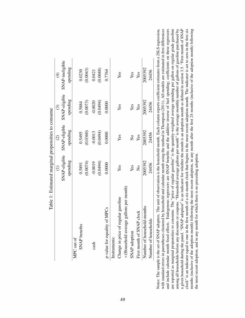
Tabl

e1:

Est

imat

edm

argi

nalp

rope

nsiti

esto

cons

ume

(1)

(2)

(3)

(4)

SNA

P-el

igib

leSN

AP-

elig

ible

SNA

P-el

igib

leSN

AP-

inel

igib

lesp

endi

ngsp

endi

ngsp

endi

ngsp

endi

ngM

PCou

tof

SNA

Pbe

nefit

s0.

5891

0.54

950.

5884

0.02

30(0

.007

4)(0

.036

0)(0

.007

3)(0

.004

3)

cash

-0.0

019

-0.0

013

-0.0

020

0.04

21(0

.049

4)(0

.049

4)(0

.049

4)(0

.068

8)

p-va

lue

fore

qual

ityof

MPC

s0.

0000

0.00

000.

0000

0.77

64In

stru

men

ts:

Cha

nge

inpr

ice

ofre

gula

rgas

olin

eY

esY

esY

esY

es×

(Hou

seho

ldav

erag

ega

llons

perm

onth

)SN

AP

adop

tion

Yes

No

Yes

Yes

Firs

tmon

thof

SNA

Pcl

ock

No

Yes

Yes

Yes

Num

bero

fhou

seho

ld-m

onth

s20

0539

220

0539

220

0539

220

0539

2N

umbe

rofh

ouse

hold

s24

456

2445

624

456

2445

6

Not

es:T

hesa

mpl

eis

the

seto

fSN

AP

adop

ters

.The

unit

ofob

serv

atio

nis

the

hous

ehol

d-m

onth

.Eac

hco

lum

nre

port

sco

effic

ient

estim

ates

from

a2S

LS

regr

essi

on,

with

stan

dard

erro

rsin

pare

nthe

ses

clus

tere

dby

hous

ehol

dan

dca

lend

arm

onth

usin

gth

em

etho

din

Tho

mps

on(2

011)

.All

mod

els

are

estim

ated

infir

stdi

ffer

ence

san

din

clud

eca

lend

arm

onth

fixed

effe

cts.

End

ogen

ous

regr

esso

rsar

eSN

AP

bene

fits

and

the

addi

tive

inve

rse

offu

elsp

endi

ng;

coef

ficie

nts

onth

ese

regr

esso

rsar

ere

port

edas

mar

gina

lpro

pens

ities

toco

nsum

e.T

he“p

rice

ofre

gula

rga

solin

e”is

the

quan

tity-

wei

ghte

dav

erag

esp

endi

ngpe

rga

llon

onre

gula

rgr

ade

gaso

line

amon

gal

lhou

seho

lds

befo

rean

ydi

scou

nts

orco

upon

s.“H

ouse

hold

aver

age

gallo

nspe

rmon

th”

isth

eav

erag

em

onth

lynu

mbe

rofg

allo

nsof

gaso

line

purc

hase

dby

agi

ven

hous

ehol

ddu

ring

the

pane

l.“S

NA

Pad

optio

n”is

anin

dica

torf

orw

heth

erth

em

onth

isan

adop

tion

mon

thas

defin

edin

sect

ion

3.5.

“Fir

stm

onth

ofSN

AP

cloc

k”is

anin

dica

tore

qual

toon

ein

the

first

mon

thof

asi

x-m

onth

cloc

kth

atbe

gins

inth

em

ostr

ecen

tado

ptio

nm

onth

.The

indi

cato

ris

sett

oze

roin

the

first

six

mon

ths

(inc

lusi

veof

the

adop

tion

mon

th)

follo

win

gth

em

ostr

ecen

tado

ptio

n,in

any

mon

thaf

ter

the

first

24m

onth

s(i

nclu

sive

ofth

ead

optio

nm

onth

)fo

llow

ing

the

mos

trec

enta

dopt

ion,

and

inan

ym

onth

forw

hich

ther

eis

nopr

eced

ing

adop

tion.

49

Tabl

e2:

Sens

itivi

tyof

estim

ated

MPC

Fto

assu

mpt

ions

abou

tret

aile

rsha

reof

spen

ding

(1)

(2)

(3)

(4)

(5)

SNA

P-el

igib

lesp

endi

ngac

ross

allr

etai

lers

MPC

Fou

tof

SNA

Pbe

nefit

s0.

5891

0.58

910.

5609

0.53

800.

1316

(0.0

074)

(0.0

074)

(0.0

075)

(0.0

075)

(0.0

089)

cash

-0.0

019

-0.0

023

-0.0

018

-0.0

014

0.00

55(0

.049

4)(0

.060

2)(0

.060

6)(0

.060

9)(0

.066

1)

p-va

lue

fore

qual

ityof

MPC

s0.

0000

0.00

000.

0000

0.00

000.

0532

Ass

umed

reta

ilers

hare

ofSN

AP-

elig

ible

spen

ding

whe

nho

useh

old

is:

Not

onSN

AP

1.00

00.

820

0.80

90.

800

0.67

1O

nSN

AP

1.00

00.

820

0.82

00.

820

0.82

0B

asis

fora

ssum

edef

fect

ofSN

AP

No

No

Hom

esca

nH

omes

can

Impo

seon

reta

ilers

hare

ofsp

endi

ngef

fect

effe

ctpo

inte

stim

ate

uppe

rbou

ndfu

ngib

ility

Num

bero

fhou

seho

ld-m

onth

s20

0539

220

0539

220

0539

220

0539

220

0539

2N

umbe

rofh

ouse

hold

s24

456

2445

624

456

2445

624

456

Not

es:T

hesa

mpl

eis

the

seto

fSN

AP

adop

ters

.The

unit

ofob

serv

atio

nis

the

hous

ehol

d-m

onth

.Eac

hco

lum

nre

port

sco

effic

ient

estim

ates

from

a2S

LS

regr

essi

on,

with

stan

dard

erro

rsin

pare

nthe

ses

clus

tere

dby

hous

ehol

dan

dca

lend

arm

onth

usin

gth

em

etho

din

Tho

mps

on(2

011)

.All

mod

els

are

estim

ated

infir

stdi

ffer

ence

san

din

clud

eca

lend

arm

onth

fixed

effe

cts.

End

ogen

ous

regr

esso

rsar

eSN

AP

bene

fits

and

the

addi

tive

inve

rse

offu

elsp

endi

ng;c

oeffi

cien

tson

thes

ere

gres

sors

are

repo

rted

asm

argi

nalp

rope

nsiti

esto

cons

ume.

Exc

lude

din

stru

men

tsar

eth

epr

oduc

toft

hepr

ice

ofre

gula

rgas

olin

ean

dho

useh

old

aver

age

gallo

nspe

rmon

th,a

ndan

indi

cato

rfor

SNA

Pad

optio

n,as

inco

lum

n(1

)oft

able

1.In

each

colu

mn,

the

depe

nden

tvar

iabl

eis

tota

lSN

AP-

elig

ible

spen

ding

acro

ssal

lret

aile

rs,c

ompu

ted

bydi

vidi

ngSN

AP-

elig

ible

spen

ding

atth

ere

taile

rby

the

“on

SNA

P”sh

are

inSN

AP

mon

ths

and

the

“not

onSN

AP”

shar

ein

othe

rm

onth

s.In

colu

mn

(1)

we

assu

me

that

allh

ouse

hold

sde

vote

allS

NA

P-el

igib

lesp

endi

ngto

the

reta

ileri

nal

lmon

ths.

Inco

lum

n(2

)we

assu

me

that

allh

ouse

hold

sde

vote

aco

nsta

ntsh

are

ofSN

AP-

elig

ible

spen

ding

toth

ere

taile

r,w

ithth

esh

are

give

nby

the

ratio

ofav

erag

eSN

AP

bene

fits

betw

een

reta

ilera

ndad

min

istr

ativ

eda

tain

onlin

eap

pend

ixta

ble

3.In

colu

mns

(3)t

hrou

gh(5

)we

assu

me

the

sam

esh

are

ofsp

endi

ngin

SNA

Pm

onth

sas

inco

lum

n(2

).In

colu

mns

(3)a

nd(4

)we

assu

me

that

the

diff

eren

cein

the

shar

eof

spen

ding

betw

een

SNA

Pm

onth

san

dno

n-SN

AP

mon

ths

iseq

ualt

oth

epo

inte

stim

ate

and

uppe

rbou

ndof

the

95pe

rcen

tcon

fiden

cein

terv

al,r

espe

ctiv

ely,

ofth

eef

fect

ofSN

AP

part

icip

atio

non

the

shar

eof

spen

ding

devo

ted

toth

epr

imar

yre

taile

rin

colu

mn

(2)

ofap

pend

ixta

ble

1.In

colu

mn

(5)

we

assu

me

that

the

shar

eof

spen

ding

inno

n-SN

AP

mon

ths

isth

ela

rges

tval

uesu

chth

atw

eca

nnot

reje

ctth

enu

llhy

poth

esis

ofan

equa

lMPC

Fbe

twee

nSN

AP

and

cash

.

50

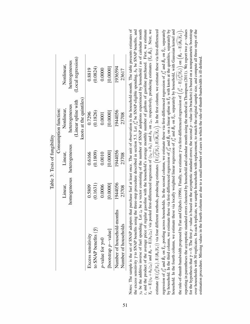
Tabl

e3:

Test

sof

fung

ibili

tyC

onsu

mpt

ion

func

tion:

Lin

ear,

Lin

ear,

Non

linea

r,N

onlin

ear,

hom

ogen

eous

hete

roge

neou

she

tero

gene

ous

hete

roge

neou

s(L

inea

rspl

ine

with

(Loc

alre

gres

sion

)kn

ots

atth

equ

intil

es)

Exc

ess

sens

itivi

ty0.

5809

0.61

660.

7296

0.88

19to

SNA

Pbe

nefit

s(γ

)(0

.163

1)(0

.180

9)(0

.182

6)(0

.082

4)p-

valu

efo

rγ=0

0.00

060.

0010

0.00

010.

0000

[boo

tstr

app−

valu

e][0

.000

0][0

.000

0][0

.000

0][0

.000

0]

Num

bero

fhou

seho

ld-m

onth

s19

4405

619

4405

619

4405

619

3659

4N

umbe

rofh

ouse

hold

s23

708

2370

823

708

2361

7

Not

es:

The

sam

ple

isth

ese

tof

SNA

Pad

opte

rsth

atpu

rcha

sefu

elat

leas

tonc

e.T

heun

itof

obse

rvat

ion

isth

eho

useh

old-

mon

th.

The

tabl

epr

esen

tses

timat

esof

the

exce

ssse

nsiti

vity

γto

SNA

Pbe

nefit

sus

ing

the

thre

e-st

eppr

oced

ure

desc

ribe

din

sect

ion

5.3.

Let

fγ itbe

SNA

P-el

igib

lesp

endi

ng,b

itbe

SNA

Pbe

nefit

s,an

dy i

tbe

the

addi

tive

inve

rse

offu

elsp

endi

ng.

Let

z itbe

ave

ctor

cons

istin

gof

the

num

ber

ofSN

AP

adop

tions

expe

rien

ced

byho

useh

old

ias

ofca

lend

arm

onth

t,an

dth

epr

oduc

tof

the

aver

age

pric

eof

regu

lar

gaso

line

with

the

hous

ehol

d’s

aver

age

mon

thly

num

ber

ofga

llons

ofga

solin

epu

rcha

sed.

Firs

t,w

ees

timat

eY i

t=

E(y

it+

b it|z

it)

and

Bit

=E

(bit|z i

t)vi

apo

oled

first

-diff

eren

ced

regr

essi

onof

(yit+

b it)

and

b it

onz it

,re

spec

tivel

y,pr

oduc

ing

estim

ates( Y i

t,B

it) .

Nex

t,w

e

estim

ate( E( fγ it|Y

it) ,E

(Bit|Y

it)) vi

afo

urdi

ffer

entm

etho

ds,p

rodu

cing

estim

ates(

E( fγ it|Y

it) ,

E

(Bit|Y

it)) .I

nth

efir

stco

lum

n,w

ees

timat

eth

ese

via

first

-diff

eren

ced

regr

essi

onof

fγ itan

dB

iton

Y it,

pool

ing

acro

ssho

useh

olds

.In

the

seco

ndco

lum

n,w

ees

timat

eth

ese

via

first

-diff

eren

ced

regr

essi

onof

fγ itan

dB

iton

Y it,

sepa

rate

lyby

hous

ehol

d.In

the

thir

dco

lum

n,w

ees

timat

eth

ese

via

first

-diff

eren

ced

regr

essi

onof

fγ itan

dB

iton

alin

ears

plin

ein

Y it

with

knot

sat

the

quin

tiles

,sep

arat

ely

byho

useh

old.

Inth

efo

urth

colu

mn,

we

estim

ate

thes

evi

alo

cally

wei

ghte

dlin

ear

regr

essi

onof

fγ itan

dB

iton

Y it,

sepa

rate

lyby

hous

ehol

d,w

ithG

auss

ian

kern

elan

d

the

rule

-of-

thum

bba

ndw

idth

prop

osed

byFa

nan

dG

ijbel

s(1

996)

.Fin

ally

,we

estim

ate

γvi

afir

st-d

iffer

ence

dre

gres

sion

of( fγ it−

E( fγ it|Y

it)) on

( Bit−

E

(Bit|Y

it)) ,

repo

rtin

gin

pare

nthe

ses

the

asym

ptot

icst

anda

rder

rors

clus

tere

dby

hous

ehol

dan

dca

lend

arm

onth

usin

gth

em

etho

din

Tho

mps

on(2

011)

.We

repo

rttw

op−

valu

esfo

rthe

hypo

thes

isth

atγ

=0.

The

first

p−va

lue

isba

sed

onth

eas

ympt

otic

stan

dard

erro

rs;t

hese

cond

p−va

lue

(in

brac

kets

)is

base

don

ano

npar

amet

ric

boot

stra

pov

erho

useh

olds

with

30re

plic

ates

.In

each

repl

icat

e,w

esa

mpl

eho

useh

olds

with

repl

acem

ent,

tom

atch

the

orig

inal

sam

ple

size

,and

com

pute

allt

hree

step

sof

the

estim

atio

npr

oced

ure.

Mis

sing

valu

esin

the

four

thco

lum

nar

edu

eto

asm

alln

umbe

rofc

ases

inw

hich

the

rule

-of-

thum

bba

ndw

idth

isill

-defi

ned.

51

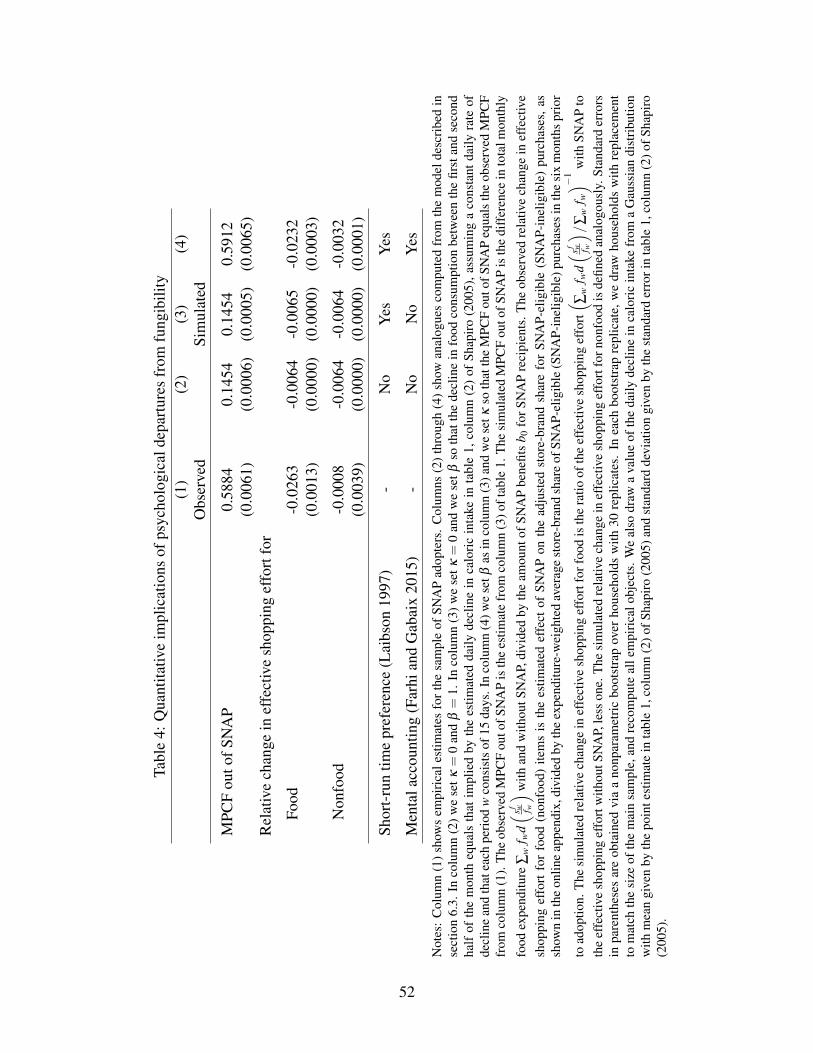
Tabl

e4:

Qua

ntita

tive

impl

icat

ions

ofps

ycho

logi

cald

epar

ture

sfr

omfu

ngib

ility

(1)

(2)

(3)

(4)

Obs

erve

dSi

mul

ated

MPC

Fou

tofS

NA

P0.

5884

0.14

540.

1454

0.59

12(0

.006

1)(0

.000

6)(0

.000

5)(0

.006

5)R

elat

ive

chan

gein

effe

ctiv

esh

oppi

ngef

fort

for

Food

-0.0

263

-0.0

064

-0.0

065

-0.0

232

(0.0

013)

(0.0

000)

(0.0

000)

(0.0

003)

Non

food

-0.0

008

-0.0

064

-0.0

064

-0.0

032

(0.0

039)

(0.0

000)

(0.0

000)

(0.0

001)

Shor

t-ru

ntim

epr

efer

ence

(Lai

bson

1997

)-

No

Yes

Yes

Men

tala

ccou

ntin

g(F

arhi

and

Gab

aix

2015

)-

No

No

Yes

Not

es:

Col

umn

(1)

show

sem

piri

cale

stim

ates

for

the

sam

ple

ofSN

AP

adop

ters

.C

olum

ns(2

)th

roug

h(4

)sh

owan

alog

ues

com

pute

dfr

omth

em

odel

desc

ribe

din

sect

ion

6.3.

Inco

lum

n(2

)we

setκ

=0

and

β=

1.In

colu

mn

(3)w

ese

tκ=

0an

dw

ese

tβso

that

the

decl

ine

info

odco

nsum

ptio

nbe

twee

nth

efir

stan

dse

cond

half

ofth

em

onth

equa

lsth

atim

plie

dby

the

estim

ated

daily

decl

ine

inca

lori

cin

take

inta

ble

1,co

lum

n(2

)of

Shap

iro

(200

5),a

ssum

ing

aco

nsta

ntda

ilyra

teof

decl

ine

and

that

each

peri

odw

cons

ists

of15

days

.In

colu

mn

(4)w

ese

tβas

inco

lum

n(3

)and

we

setκ

soth

atth

eM

PCF

outo

fSN

AP

equa

lsth

eob

serv

edM

PCF

from

colu

mn

(1).

The

obse

rved

MPC

Fou

tofS

NA

Pis

the

estim

ate

from

colu

mn

(3)o

ftab

le1.

The

sim

ulat

edM

PCF

outo

fSN

AP

isth

edi

ffer

ence

into

talm

onth

ly

food

expe

nditu

re∑

wf w

d( sf w f w

) with

and

with

outS

NA

P,di

vide

dby

the

amou

ntof

SNA

Pbe

nefit

sb 0

forS

NA

Pre

cipi

ents

.The

obse

rved

rela

tive

chan

gein

effe

ctiv

esh

oppi

ngef

fort

for

food

(non

food

)ite

ms

isth

ees

timat

edef

fect

ofSN

AP

onth

ead

just

edst

ore-

bran

dsh

are

for

SNA

P-el

igib

le(S

NA

P-in

elig

ible

)pu

rcha

ses,

assh

own

inth

eon

line

appe

ndix

,div

ided

byth

eex

pend

iture

-wei

ghte

dav

erag

est

ore-

bran

dsh

are

ofSN

AP-

elig

ible

(SN

AP-

inel

igib

le)p

urch

ases

inth

esi

xm

onth

spr

ior

toad

optio

n.T

hesi

mul

ated

rela

tive

chan

gein

effe

ctiv

esh

oppi

ngef

fort

forf

ood

isth

era

tioof

the

effe

ctiv

esh

oppi

ngef

fort( ∑

wf w

d( sf w f w

) /∑

wf w) −1 w

ithSN

AP

toth

eef

fect

ive

shop

ping

effo

rtw

ithou

tSN

AP,

less

one.

The

sim

ulat

edre

lativ

ech

ange

inef

fect

ive

shop

ping

effo

rtfo

rnon

food

isde

fined

anal

ogou

sly.

Stan

dard

erro

rsin

pare

nthe

ses

are

obta

ined

via

ano

npar

amet

ric

boot

stra

pov

erho

useh

olds

with

30re

plic

ates

.In

each

boot

stra

pre

plic

ate,

we

draw

hous

ehol

dsw

ithre

plac

emen

tto

mat

chth

esi

zeof

the

mai

nsa

mpl

e,an

dre

com

pute

alle

mpi

rica

lobj

ects

.We

also

draw

ava

lue

ofth

eda

ilyde

clin

ein

calo

ric

inta

kefr

oma

Gau

ssia

ndi

stri

butio

nw

ithm

ean

give

nby

the

poin

test

imat

ein

tabl

e1,

colu

mn

(2)o

fSha

piro

(200

5)an

dst

anda

rdde

viat

ion

give

nby

the

stan

dard

erro

rin

tabl

e1,

colu

mn

(2)o

fSha

piro

(200

5).

52

Figure 1: In-state earnings and number of children before and after SNAP adoptionPanel A: In-state earnings and unemployment insurance benefits

400

450

500

550

600

650

Ave

rage

mon

thly

in−

stat

e ea

rnin

gs a

nd U

I ben

efits

($)

−4 40Quarters relative to SNAP adoption

Panel B: Number of children under five years of age

.16

.18

.2.2

2.2

4N

umbe

r of

chi

ldre

n un

der

five

year

s of

age

−12 120Months relative to SNAP adoption

Notes: Data are from Rhode Island administrative records from October 2004 through June 2016. Seesection 2.1 for details on sample definition and variable construction. Each panel plots coefficients from aregression of the dependent variable on a vector of lead and lagged indicators for periods relative to SNAPadoption, defined as the first period in which the household receives SNAP. The period immediately prior toadoption (“-1”) is the omitted category. Each regression includes time period fixed effects, household fixedeffects, and indicators for observations more than one year before or after adoption. In panel A, a time periodis a calendar quarter and the unit of analysis is a household-quarter. In panel B, a time period is a monthand the unit of analysis is the household-month. In both panels, the error bars are ±2 coefficient standarderrors and standard errors are clustered by household. Dotted lines show the sample mean of the dependentvariable across observations within one year (4 quarters or 12 months) of SNAP adoption. Each coefficientseries is shifted by a constant so that the observation-count-weighted mean of the regression coefficients isequal to the sample mean of the corresponding dependent variable.

53

Figure 2: Distribution of lengths of SNAP spells

0.0

5.1

.15

.2.2

5F

ract

ion

of S

NA

P s

pells

0 6 12 18 24 30 36SNAP spell length (months)

Notes: Data are from Rhode Island administrative records from October 2004 through June 2016. Seesection 2.1 for details on sample definition and variable construction. The plot shows a histogram of thedistribution of SNAP spell lengths, where a spell is defined as a set of consecutive months in which thehousehold is entitled to a SNAP benefit in each month according to state program records. Spells longerthan 36 months are excluded from the sample.

54

Figure 3: Inferring SNAP adoption from single-retailer data

.2.4

.6.8

1P

r(S

NA

P a

dopt

ion

with

in tw

o m

onth

s of

tran

sitio

n)

1 2 3 4 5 6 7 8 9 10 11 12Radius of transition period (months)

All householdsHouseholds who mainly spend SNAP at the Rhode Island Retailer

Notes: Data are from Rhode Island EBT transaction records from September 2012 through October 2015.See section 2.1 for details on sample definition and variable construction. The figure plots the fraction oftransition periods of a given radius in which the household newly enrolled in SNAP within two months ofthe start of SNAP spending at the Rhode Island Retailer. We define new enrollment as the receipt of at least$10 in SNAP benefits following a period of at least three consecutive months with no benefit. A transitionperiod of radius K is a period in which a household exhibits K consecutive months without SNAP spendingat the Rhode Island Retailer followed by K consecutive months with SNAP spending at the Rhode IslandRetailer. Households who mainly spend SNAP at the Rhode Island Retailer are those who spend at least halfof their total EBT expenditures between September 2012 and October 2015 at the Rhode Island Retailer.

55

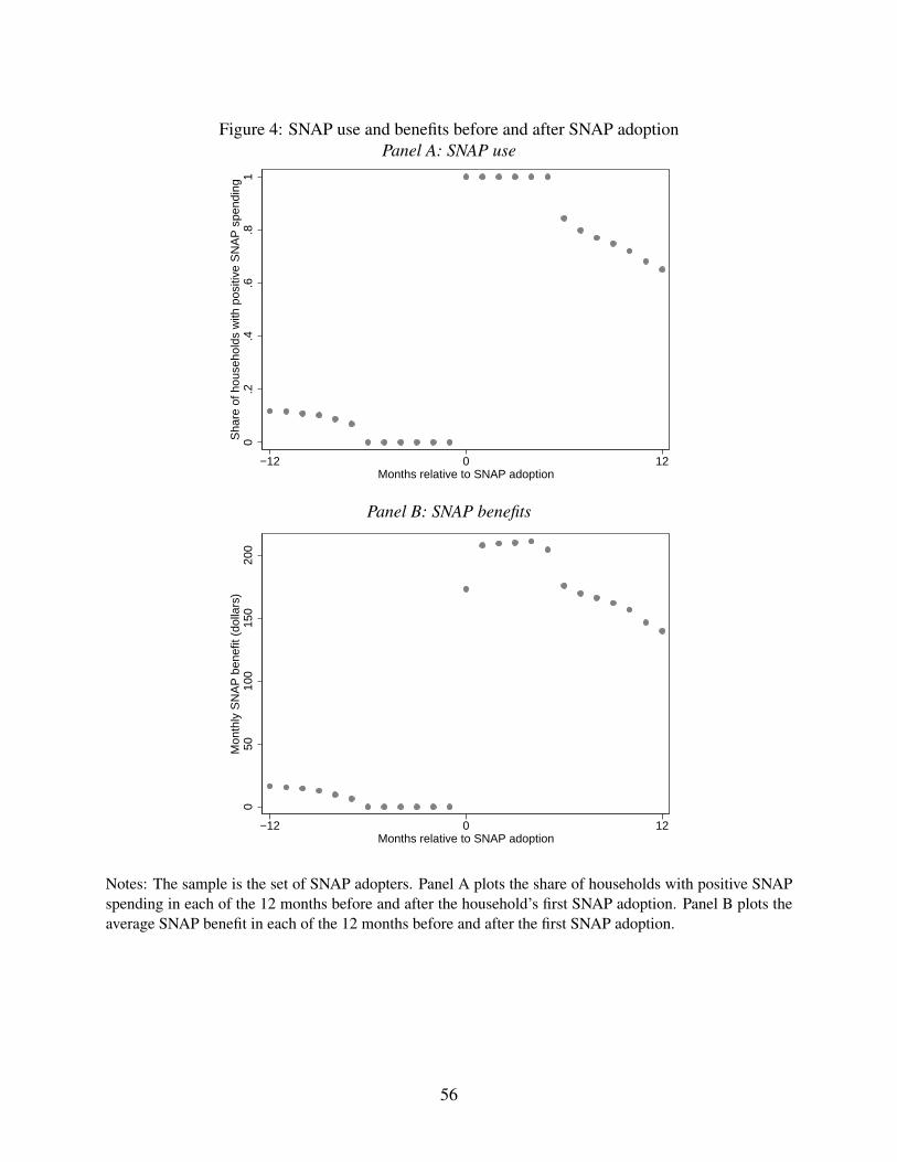
Figure 4: SNAP use and benefits before and after SNAP adoptionPanel A: SNAP use

0.2

.4.6

.81

Sha

re o

f hou

seho

lds

with

pos

itive

SN

AP

spe

ndin

g

−12 120Months relative to SNAP adoption

Panel B: SNAP benefits

050

100

150

200

Mon

thly

SN

AP

ben

efit

(dol

lars

)

−12 120Months relative to SNAP adoption

Notes: The sample is the set of SNAP adopters. Panel A plots the share of households with positive SNAPspending in each of the 12 months before and after the household’s first SNAP adoption. Panel B plots theaverage SNAP benefit in each of the 12 months before and after the first SNAP adoption.

56

Figure 5: Monthly expenditure before and after SNAP adoptionPanel A: SNAP-eligible spending

350

400

450

500

Mon

thly

exp

endi

ture

(do

llars

)

−12 120Months relative to SNAP adoption

Panel B: SNAP-ineligible spending

5010

015

020

0M

onth

ly e

xpen

ditu

re (

dolla

rs)

−12 120Months relative to SNAP adoption

Notes: Each figure plots coefficients from a regression of SNAP-eligible or SNAP-ineligible spending ona vector of lead and lagged indicators for month relative to the household’s first SNAP adoption, with themonth prior to SNAP adoption (“-1”) as the omitted category. The unit of observation for each regressionis the household-month and the sample is the set of SNAP adopters. Error bars are ±2 coefficient standarderrors. Standard errors are clustered by household. Each regression includes calendar month fixed effects,household fixed effects, and two indicators for observations before and after 12 months of SNAP adoption.The dotted lines show the sample mean of household monthly expenditure across observations within 12months of SNAP adoption. Each coefficient series is shifted by a constant so that the observation-count-weighted mean of the regression coefficients is equal to the sample mean of the corresponding dependentvariable.

57

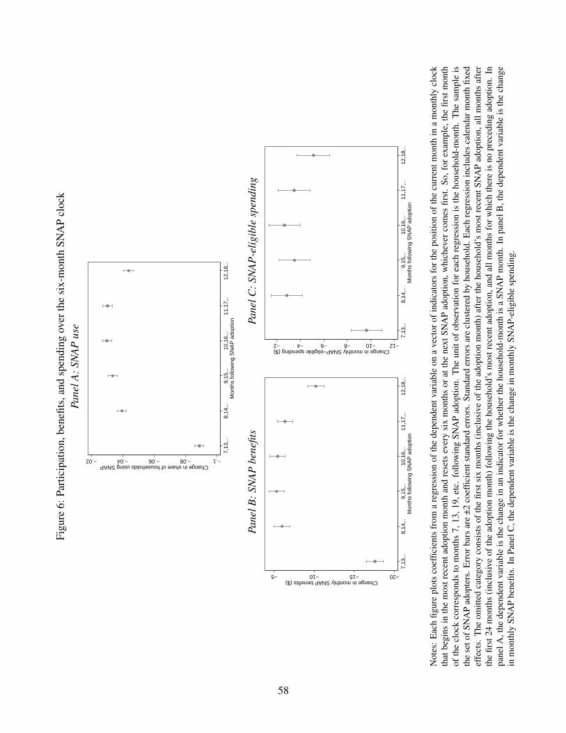
Figu

re6:

Part

icip

atio

n,be

nefit

s,an

dsp

endi

ngov

erth

esi

x-m

onth

SNA

Pcl

ock

Pane

lA:S

NA

Pus

e

−.1−.08−.06−.04−.02Change in share of households using SNAP

7,13

,..8,

14,..

9,15

,..10

,16,

..11

,17,

..12

,18,

..M

onth

s fo

llow

ing

SN

AP

ado

ptio

n

Pane

lB:S

NA

Pbe

nefit

sPa

nelC

:SN

AP

-elig

ible

spen

ding

−20−15−10−5Change in monthly SNAP benefits ($)

7,13

,..8,

14,..

9,15

,..10

,16,

..11

,17,

..12

,18,

..M

onth

s fo

llow

ing

SN

AP

ado

ptio

n

−12−10−8−6−4−2Change in monthly SNAP−eligible spending ($)

7,13

,..8,

14,..

9,15

,..10

,16,

..11

,17,

..12

,18,

..M

onth

s fo

llow

ing

SN

AP

ado

ptio

n

Not

es:

Eac

hfig

ure

plot

sco

effic

ient

sfr

oma

regr

essi

onof

the

depe

nden

tvar

iabl

eon

ave

ctor

ofin

dica

tors

fort

hepo

sitio

nof

the

curr

entm

onth

ina

mon

thly

cloc

kth

atbe

gins

inth

em

ostr

ecen

tado

ptio

nm

onth

and

rese

tsev

ery

six

mon

ths

orat

the

next

SNA

Pad

optio

n,w

hich

ever

com

esfir

st.

So,f

orex

ampl

e,th

efir

stm

onth

ofth

ecl

ock

corr

espo

nds

tom

onth

s7,

13,1

9,et

c.fo

llow

ing

SNA

Pad

optio

n.T

heun

itof

obse

rvat

ion

for

each

regr

essi

onis

the

hous

ehol

d-m

onth

.T

hesa

mpl

eis

the

seto

fSN

AP

adop

ters

.Err

orba

rsar

e±2

coef

ficie

ntst

anda

rder

rors

.Sta

ndar

der

rors

are

clus

tere

dby

hous

ehol

d.E

ach

regr

essi

onin

clud

esca

lend

arm

onth

fixed

effe

cts.

The

omitt

edca

tego

ryco

nsis

tsof

the

first

six

mon

ths

(inc

lusi

veof

the

adop

tion

mon

th)

afte

rth

eho

useh

old’

sm

ostr

ecen

tSN

AP

adop

tion,

allm

onth

saf

ter

the

first

24m

onth

s(i

nclu

sive

ofth

ead

optio

nm

onth

)fol

low

ing

the

hous

ehol

d’s

mos

trec

enta

dopt

ion,

and

allm

onth

sfo

rwhi

chth

ere

isno

prec

edin

gad

optio

n.In

pane

lA,t

hede

pend

entv

aria

ble

isth

ech

ange

inan

indi

cato

rfor

whe

ther

the

hous

ehol

d-m

onth

isa

SNA

Pm

onth

.In

pane

lB,t

hede

pend

entv

aria

ble

isth

ech

ange

inm

onth

lySN

AP

bene

fits.

InPa

nelC

,the

depe

nden

tvar

iabl

eis

the

chan

gein

mon

thly

SNA

P-el

igib

lesp

endi

ng.

58

Figure 7: Monthly SNAP benefits and SNAP-eligible spending around benefit changesPanel A: Administrative data for retailer states

220

240

260

280

300

Ave

rage

mon

thly

SN

AP

ben

efit

per

hous

ehol

d (d

olla

rs)

Farm Bill ARRA

Jan−2008 Dec−2009Oct−2008 Apr−2009

Panel B: Retailer data

260

290

320

350

380

Mon

thly

SN

AP

ben

efits

(do

llars

)

430

460

490

520

550

Mon

thly

SN

AP

−el

igib

le s

pend

ing

(dol

lars

)

Farm Bill ARRA

Jan−2008 Dec−2009Oct−2008 Apr−2009

SNAP−eligible spending SNAP benefits

Notes: Panel A plots the average monthly SNAP benefit per household between January 2008 and December 2009from administrative data. The series was obtained by weighing the average monthly SNAP benefit per householdfor each state (according to data from the United States Department of Agriculture Food and Nutrition Service viahttp://www.fns.usda.gov/sites/default/files/pd/SNAPZip69throughCurrent.zip as of May 2017) bythe number of retailer households with at least one SNAP month. Panel B plots coefficients from a regression ofSNAP benefits and SNAP-eligible spending on interactions between the share of calendar months between February2006 and December 2007 during which each household used SNAP and calendar month indicators, with the January2008 interaction normalized to zero. The sample includes all households in the retailer panel with at least one SNAPmonth. The unit of observation is the household-month and only months from January 2008 to December 2009 areincluded in the regression. Error bars and shaded region represent ±2 coefficient standard errors. Standard errors areclustered by household. Each regression includes household and calendar month fixed effects. Each coefficient seriesis seasonally adjusted by subtracting from each coefficient the corresponding coefficient from an auxiliary regressionof the dependent variable on interactions between the share of months between February 2006 and December 2007during which each household used SNAP and year and seasonal month indicators. The auxiliary regressions includehousehold, year, and seasonal month fixed effects and are estimated using only data from January 2010 to December2012. Each coefficient series is shifted by a constant so that the observation-count-weighted mean of the regressioncoefficients is equal to the sample mean of the corresponding dependent variable among households who used SNAPin every month between February 2006 and December 2007. In both panels, vertical lines at October 2008 and April2009 denote the implementation dates of changes in SNAP benefits due to the Farm Bill and American Recovery andReinvestment Act (ARRA), respectively.

59

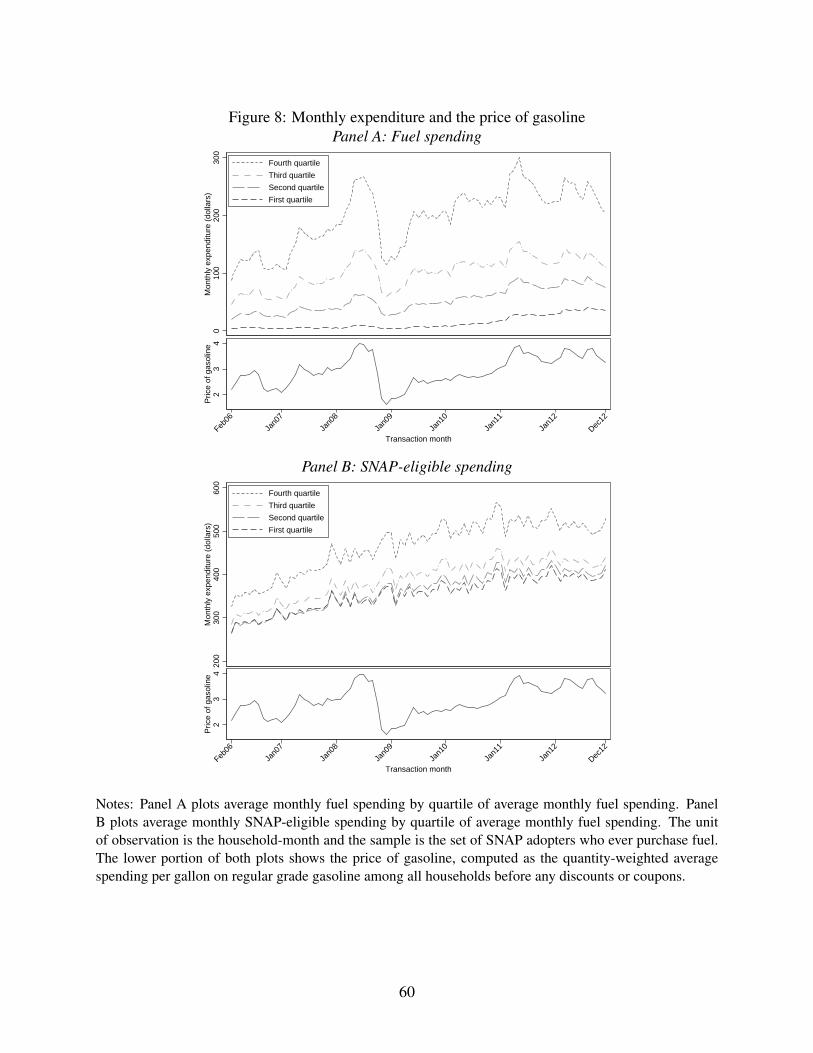
Figure 8: Monthly expenditure and the price of gasolinePanel A: Fuel spending

010

020

030

0M

onth

ly e

xpen

ditu

re (

dolla

rs)

Fourth quartile

Third quartile

Second quartile

First quartile

23

4P

rice

of g

asol

ine

Feb06

Jan0

7

Jan0

8

Jan0

9

Jan1

0

Jan1

1

Jan1

2

Dec12

Transaction month

Panel B: SNAP-eligible spending

200

300

400

500

600

Mon

thly

exp

endi

ture

(do

llars

)

Fourth quartile

Third quartile

Second quartile

First quartile

23

4P

rice

of g

asol

ine

Feb06

Jan0

7

Jan0

8

Jan0

9

Jan1

0

Jan1

1

Jan1

2

Dec12

Transaction month

Notes: Panel A plots average monthly fuel spending by quartile of average monthly fuel spending. PanelB plots average monthly SNAP-eligible spending by quartile of average monthly fuel spending. The unitof observation is the household-month and the sample is the set of SNAP adopters who ever purchase fuel.The lower portion of both plots shows the price of gasoline, computed as the quantity-weighted averagespending per gallon on regular grade gasoline among all households before any discounts or coupons.

60

Figure 9: Store-brand share before and after SNAP adoptionPanel A: SNAP-eligible products

.33

.335

.34

.345

Adj

uste

d st

ore−

bran

d sh

are

−12 120Months relative to SNAP adoption

Panel B: SNAP-ineligible products

.225

.23

.235

.24

Adj

uste

d st

ore−

bran

d sh

are

−12 120Months relative to SNAP adoption

Notes: Each figure plots coefficients from a regression of adjusted store-brand share of expenditures on avector of lead and lagged indicators for month relative to the household’s first SNAP adoption, with themonth prior to SNAP adoption (“-1”) as the omitted category. The unit of observation for each regressionis the household-month and the sample is the set of SNAP adopters. Error bars are ±2 coefficient standarderrors. Standard errors are clustered by household. Each regression includes calendar month fixed effects,household fixed effects, and two indicators for observations before and after 12 months of SNAP adoption.The dotted line shows the sample mean of the store-brand share of expenditure across observations within12 months of SNAP adoption. Each coefficient series is shifted by a constant so that the observation-count-weighted mean of the regression coefficients is equal to the sample mean of the store-brand share ofexpenditure in the given SNAP eligibility group.

61

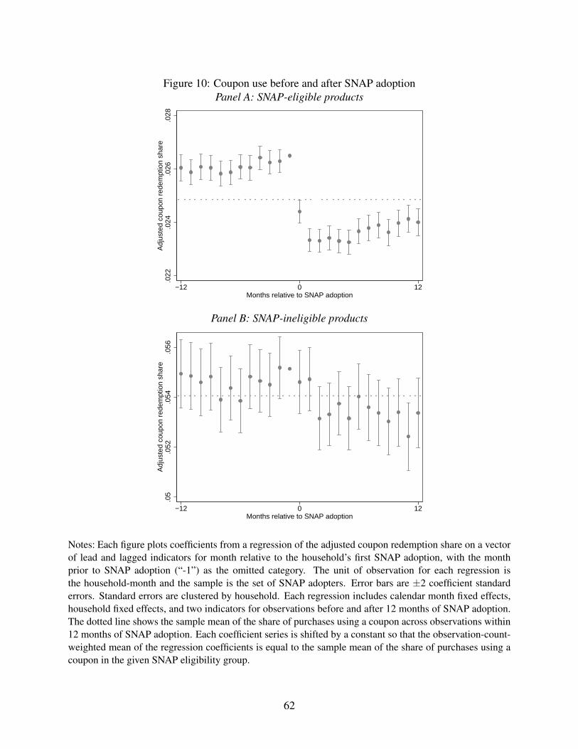
Figure 10: Coupon use before and after SNAP adoptionPanel A: SNAP-eligible products

.022

.024

.026

.028

Adj

uste

d co

upon

red

empt

ion

shar

e

−12 120Months relative to SNAP adoption

Panel B: SNAP-ineligible products

.05

.052

.054

.056

Adj

uste

d co

upon

red

empt

ion

shar

e

−12 120Months relative to SNAP adoption

Notes: Each figure plots coefficients from a regression of the adjusted coupon redemption share on a vectorof lead and lagged indicators for month relative to the household’s first SNAP adoption, with the monthprior to SNAP adoption (“-1”) as the omitted category. The unit of observation for each regression isthe household-month and the sample is the set of SNAP adopters. Error bars are ±2 coefficient standarderrors. Standard errors are clustered by household. Each regression includes calendar month fixed effects,household fixed effects, and two indicators for observations before and after 12 months of SNAP adoption.The dotted line shows the sample mean of the share of purchases using a coupon across observations within12 months of SNAP adoption. Each coefficient series is shifted by a constant so that the observation-count-weighted mean of the regression coefficients is equal to the sample mean of the share of purchases using acoupon in the given SNAP eligibility group.

62

Appendix Table 1: Relationship between SNAP status and primary retailer share of expendituresin the Nielsen Homescan Consumer Panel

Share of SNAP-eligible expenditure in primary retailer(1) (2) (3) (4)

Primary retailer type All Grocery Discount store or Otherwarehouse club

On SNAP 0.0035 0.0111 -0.0106 -0.0112(0.0036) (0.0044) (0.0063) (0.0211)

Number of households 4407 2904 1345 158Number of household-quarters 24198 16058 7309 831Dependent variable:Mean 0.515 0.512 0.535 0.398Within-household standard deviation 0.177 0.175 0.175 0.222

Notes: Data come from the Nielsen Homescan Consumer Panel and the Homescan Panel OmnibusSurvey, as described in appendix A. The unit of observation is the household-quarter. Standarderrors in parentheses are clustered by household. Each column reports results from a linear regres-sion with household and calendar quarter fixed effects. The dependent variable, “Share of SNAP-eligible expenditure in primary retailer,” is the share of SNAP-eligible spending at the household’sprimary retailer, defined as the retail chain in which the household spends the most on SNAP-eligible items across all quarters in which the household is observed in the Nielsen HomescanConsumer Panel. Column (1) includes all households regardless of the primary retailer. Columns(2) to (4) restrict the sample, respectively, to households whose primary retailer is a grocery storechain, a discount store or warehouse club chain, or another type of retailer. The key independentvariable, “On SNAP”, is an indicator for whether the household reports being on SNAP in thecurrent quarter. Household-quarters with missing values of the “On SNAP” indicator are excludedfrom the sample. Households are included in the sample if they report being on SNAP in at leastone survey response and report not being on SNAP in at least one survey response.

63

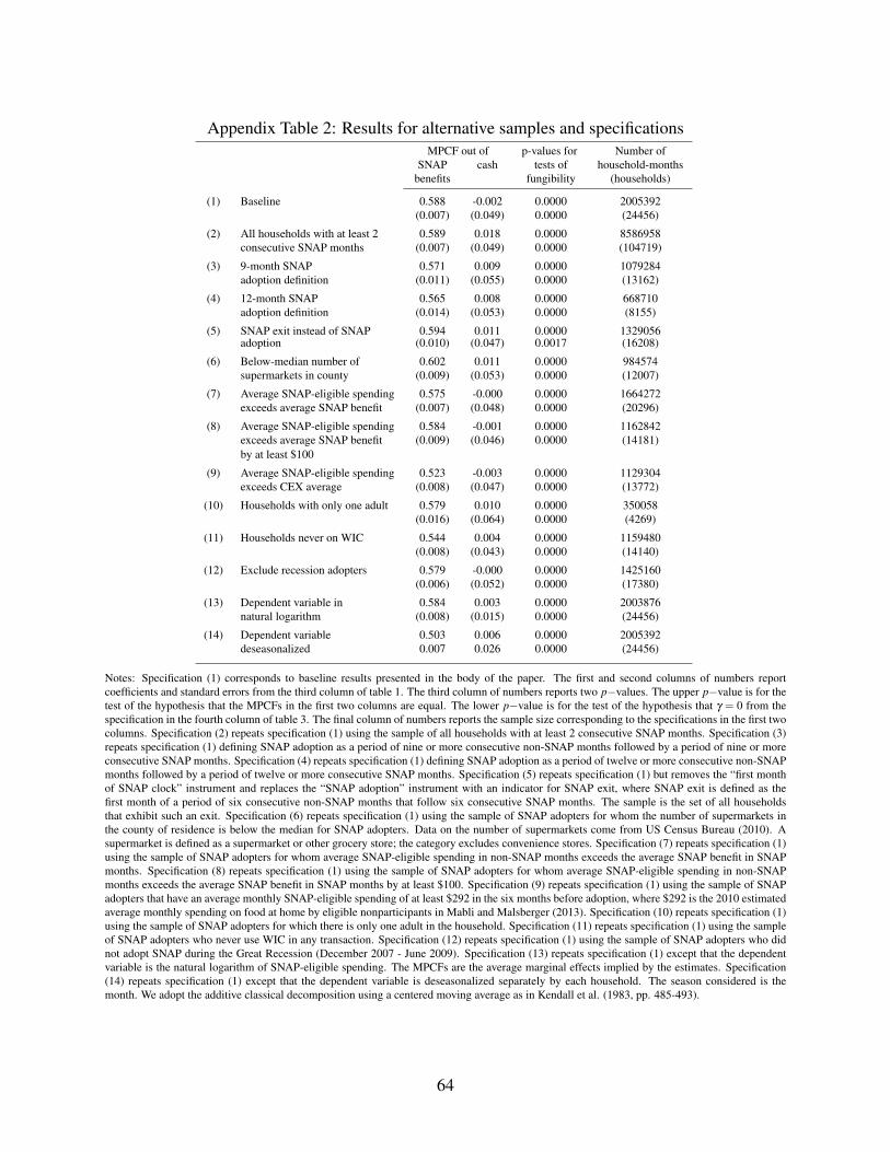
Appendix Table 2: Results for alternative samples and specificationsMPCF out of p-values for Number of

SNAP cash tests of household-monthsbenefits fungibility (households)

(1) Baseline 0.588 -0.002 0.0000 2005392(0.007) (0.049) 0.0000 (24456)

(2) All households with at least 2 0.589 0.018 0.0000 8586958consecutive SNAP months (0.007) (0.049) 0.0000 (104719)

(3) 9-month SNAP 0.571 0.009 0.0000 1079284adoption definition (0.011) (0.055) 0.0000 (13162)

(4) 12-month SNAP 0.565 0.008 0.0000 668710adoption definition (0.014) (0.053) 0.0000 (8155)

(5) SNAP exit instead of SNAP 0.594 0.011 0.0000 1329056adoption (0.010) (0.047) 0.0017 (16208)

(6) Below-median number of 0.602 0.011 0.0000 984574supermarkets in county (0.009) (0.053) 0.0000 (12007)

(7) Average SNAP-eligible spending 0.575 -0.000 0.0000 1664272exceeds average SNAP benefit (0.007) (0.048) 0.0000 (20296)

(8) Average SNAP-eligible spending 0.584 -0.001 0.0000 1162842exceeds average SNAP benefit (0.009) (0.046) 0.0000 (14181)by at least $100

(9) Average SNAP-eligible spending 0.523 -0.003 0.0000 1129304exceeds CEX average (0.008) (0.047) 0.0000 (13772)

(10) Households with only one adult 0.579 0.010 0.0000 350058(0.016) (0.064) 0.0000 (4269)

(11) Households never on WIC 0.544 0.004 0.0000 1159480(0.008) (0.043) 0.0000 (14140)

(12) Exclude recession adopters 0.579 -0.000 0.0000 1425160(0.006) (0.052) 0.0000 (17380)

(13) Dependent variable in 0.584 0.003 0.0000 2003876natural logarithm (0.008) (0.015) 0.0000 (24456)

(14) Dependent variable 0.503 0.006 0.0000 2005392deseasonalized 0.007 0.026 0.0000 (24456)

Notes: Specification (1) corresponds to baseline results presented in the body of the paper. The first and second columns of numbers reportcoefficients and standard errors from the third column of table 1. The third column of numbers reports two p−values. The upper p−value is for thetest of the hypothesis that the MPCFs in the first two columns are equal. The lower p−value is for the test of the hypothesis that γ = 0 from thespecification in the fourth column of table 3. The final column of numbers reports the sample size corresponding to the specifications in the first twocolumns. Specification (2) repeats specification (1) using the sample of all households with at least 2 consecutive SNAP months. Specification (3)repeats specification (1) defining SNAP adoption as a period of nine or more consecutive non-SNAP months followed by a period of nine or moreconsecutive SNAP months. Specification (4) repeats specification (1) defining SNAP adoption as a period of twelve or more consecutive non-SNAPmonths followed by a period of twelve or more consecutive SNAP months. Specification (5) repeats specification (1) but removes the “first monthof SNAP clock” instrument and replaces the “SNAP adoption” instrument with an indicator for SNAP exit, where SNAP exit is defined as thefirst month of a period of six consecutive non-SNAP months that follow six consecutive SNAP months. The sample is the set of all householdsthat exhibit such an exit. Specification (6) repeats specification (1) using the sample of SNAP adopters for whom the number of supermarkets inthe county of residence is below the median for SNAP adopters. Data on the number of supermarkets come from US Census Bureau (2010). Asupermarket is defined as a supermarket or other grocery store; the category excludes convenience stores. Specification (7) repeats specification (1)using the sample of SNAP adopters for whom average SNAP-eligible spending in non-SNAP months exceeds the average SNAP benefit in SNAPmonths. Specification (8) repeats specification (1) using the sample of SNAP adopters for whom average SNAP-eligible spending in non-SNAPmonths exceeds the average SNAP benefit in SNAP months by at least $100. Specification (9) repeats specification (1) using the sample of SNAPadopters that have an average monthly SNAP-eligible spending of at least $292 in the six months before adoption, where $292 is the 2010 estimatedaverage monthly spending on food at home by eligible nonparticipants in Mabli and Malsberger (2013). Specification (10) repeats specification (1)using the sample of SNAP adopters for which there is only one adult in the household. Specification (11) repeats specification (1) using the sampleof SNAP adopters who never use WIC in any transaction. Specification (12) repeats specification (1) using the sample of SNAP adopters who didnot adopt SNAP during the Great Recession (December 2007 - June 2009). Specification (13) repeats specification (1) except that the dependentvariable is the natural logarithm of SNAP-eligible spending. The MPCFs are the average marginal effects implied by the estimates. Specification(14) repeats specification (1) except that the dependent variable is deseasonalized separately by each household. The season considered is themonth. We adopt the additive classical decomposition using a centered moving average as in Kendall et al. (1983, pp. 485-493).

64