Embed Size (px)
Citation preview
Chapter 9
How are digital TV programs compressed to
allow broadcasting?
The raw bit rate of a studio video sequence is 166 Mbps whereas the
capacity of a terrestrial TV broadcasting channel is around 20 Mbps.
Ferran Marqués(º), Manuel Menezes(*), Javier Ruiz(º)
(º) Universitat Politècnica de Catalunya, Spain
(*) Instituto Superior de Ciências do Trabalho e da Empresa, Portugal.
In 1982, the CCIR defined a standard for encoding interlaced analogue
video signals in digital form mainly for studio applications. The current
name of this standard is ITU-R BT.601 (ITU 1983). Following this stan-
dard, a video signal sampled at 13.5 MHz, with a 4:2:2 sampling format
(double number of samples for the luminance component than for the two
chrominance components) and quantized with 8 bits per component pro-
duces a raw bit rate of 216 Mbps. This rate can be reduced by removing
the blanking intervals present in the interlaced analogue signal leading to a
bit rate of 166 Mbps, which is still a figure far above the main capacity of
usual transmission channels or storage devices.
Bringing digital video from its source (typically, a camera) to its desti-
nation (a display) involves a chain of processes, among which compression
(encoding) and decompression (decoding) are the key ones. In these
processes, bandwidth intensive digital video is first reduced to a managea-
ble size for transmission or storage, and then reconstructed for display.
2 F. Marqués, M. Menezes, J. Ruiz
This way, video compression allows using digital video in transmission
and storage environments that would not support uncompressed video.
In the last years, several image and video coding standards have been
proposed for various applications such as JPEG for still image coding (see
Chapter 8), H.263 for low-bit rate video communications, MPEG1 for sto-
rage media applications, MPEG2 for broadcasting and general high quality
video application, MPEG4 for streaming video and interactive multimedia
applications or H.264 for high compression requests. In this Chapter, we
describe the basic concepts of video coding that are common to these stan-
dards.
9.1 Background – Motion estimation
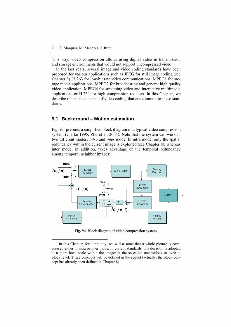
Fig. 9.1 presents a simplified block diagram of a typical video compression
system (Clarke 1995, Zhu et al. 2005). Note that the system can work in
two different modes: intra and inter mode. In intra mode, only the spatial
redundancy within the current image is exploited (see Chapter 8), whereas
inter mode, in addition, takes advantage of the temporal redundancy
among temporal neighbor images1.
Fig. 9.1 Block diagram of video compression system.
1 In this Chapter, for simplicity, we will assume that a whole picture is com-
pressed either in intra or inter mode. In current standards, this decision is adopted
at a more local scale within the image: at the so-called macroblock or even at
block level. These concepts will be defined in the sequel (actually, the block con-
cept has already been defined in Chapter 8)
How are digital TV programs compressed to allow broadcasting? 3
Let us start analyzing the system in intra mode. This is the mode used,
for instance, for the first image in a video sequence. In intra mode, the im-
age is handled as it is described in Chapter 8. Initially, a transform is ap-
plied to it in order to decorrelate its information2. The image is initially
partitioned into blocks of 8x8 pixels and the DCT transform is separately
applied on the various blocks (Noll and Jayant 1984). The transformed
coefficients are scalar quantized (Gersho and Gray 1993) taking into ac-
count the different relevancy for the human visual system of the various
DCT coefficients. Quantized coefficients are zigzag scanned and entropy
coded (Cover and Thomas 1991) in order to be efficiently transmitted.
The quantized data representing the intra mode encoded image is used in
the video coding system to provide the encoder with the same information
that will be available at the decoder side; that is, a replica of the decoded
image3. This way, a decoder is embedded in the transmitter and, through
the inverse quantization and the inverse transform, the decoded image is
obtained. This image is stored in the Frame Storage and will be used in the
coding of future frames.
This image is represented as ˆ( , , 1)I i j n where the symbol „^‟ denotes
that it is not the original frame but a decoded one. Moreover, since the sys-
tem typically has already started coding the following frame in the se-
quence, this frame is stored as belonging to time instant n – 1 (and this is
the reason for including a delay in the block diagram).
Now, we can analyze the behavior of the system in inter mode. The first
step is to exploit the temporal redundancy between previously decoded
images and the current frame. For simplicity, we are going to assume in
this initial part of the Chapter that only the previous decoded image is used
for exploiting the temporal redundancy in the video sequence. In subse-
quent Sections we will see that the Frame Storage may contain several
other decoded frames to be used in this step.
The previous decoded frame is used to estimate the current frame. To-
wards this goal, the Motion Estimation block computes the motion in the
scene; that is, a motion field is estimated, which assigns to each pixel in
the current frame a motion vector (dx, dy) representing the displacement
that this pixel has suffered with respect to the previous frame. The infor-
mation in this motion field is part of the new, more compact representation
2 In recent standards such as H.264 (Sullivan and Wiegand 2005), several other
intra mode decorrelation techniques are proposed, based on prediction. 3 Note that the quantization step very likely will introduce losses in the process
and, therefore, the decoded image is not equal to the original one.
4 F. Marqués, M. Menezes, J. Ruiz
of the video sequence and, therefore, it is entropy encoded and transmit-
ted4.
Based on this motion field and on the previous decoded frame, the Mo-
tion Compensation block produces an estimate of the current image
( , , )I i j n . This estimated image has been obtained applying motion infor-
mation to a reference image and, thus, it is commonly known as the motion
compensated image at time instant n. In this Chapter, motion compensated
images are denoted by the symbol „~‟.
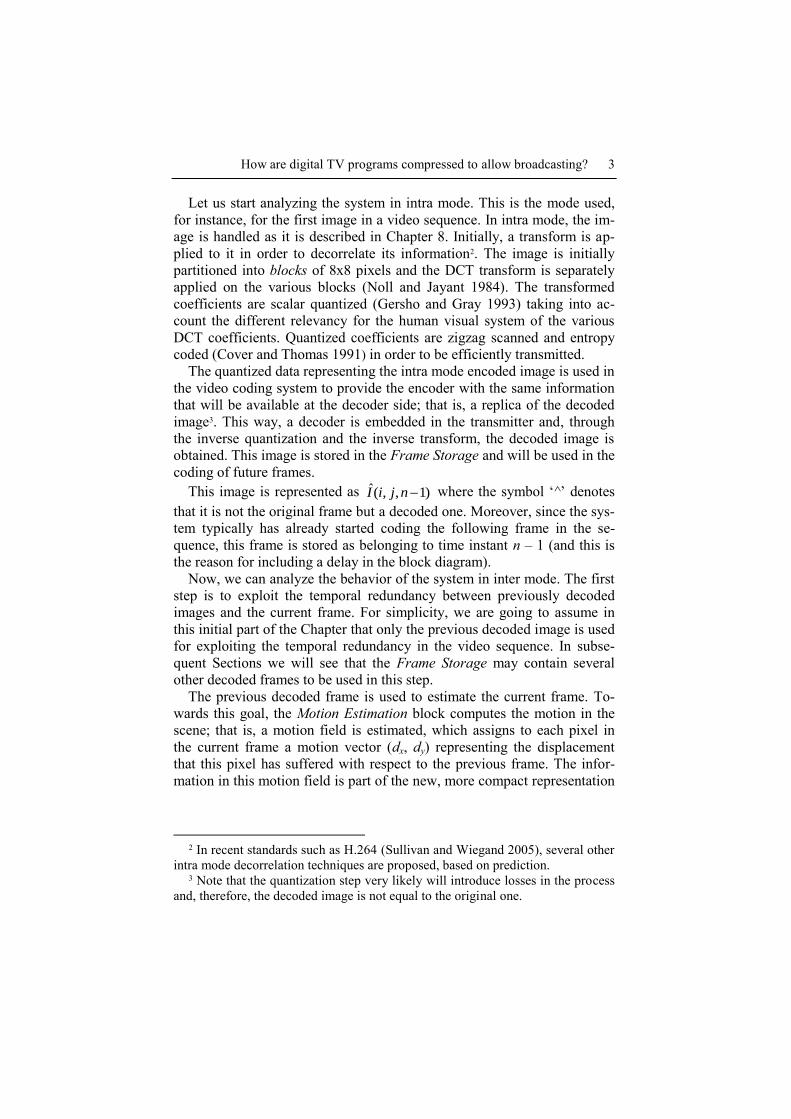
The system then subtracts the motion compensated image from the orig-
inal image, both at time n. The result is the so-called motion compensated
error image and contains all the information from the current image that
has not been correctly estimated using the information in the previous de-
coded image. These concepts are illustrated in Fig. 9.2.
(a) (b)
(c) (d) (e)
Fig. 9.2 (a) Original frame #12 of the Stefan sequence, (b) Original frame #10 of
the sequence Stefan, (c) Motion field estimated between the previous images. For
visualization purposes, only a motion vector for each 16x16 pixels area is
represented, (d) Estimation of frame #12 obtained as motion compensation of im-
age #10 using the previous motion field, (e) Motion compensated error image at
frame #12. For visualization purposes, an offset of 128 has been added to the error
image pixels, which have been afterwards conveniently scaled.
4 As it will be discussed in Section 9.1.2, this information typically does not re-
quire quantization.
How are digital TV programs compressed to allow broadcasting? 5
The motion compensated error image is now handled as an original im-
age in intra mode (or in a still image coding system, see Chapter 8). That
is, the information in the image is decorrelated (Direct Transform) typical-
ly using a DCT block transform, then the transform values are scalar quan-
tized (Quantization) and finally, quantized coefficients are entropy en-
coded (Entropy Encoder) and transmitted.
As previously, the encoding system contains an embedded decoder that
allows the transmitter to use the same decoded frames that will be used at
the receiver side5. In this case, the reconstruction of the decoded image
implies adding the quantized error to the motion compensated image and
this is the image which is stored in the Frame Storage to be used as refer-
ence for subsequent frames.
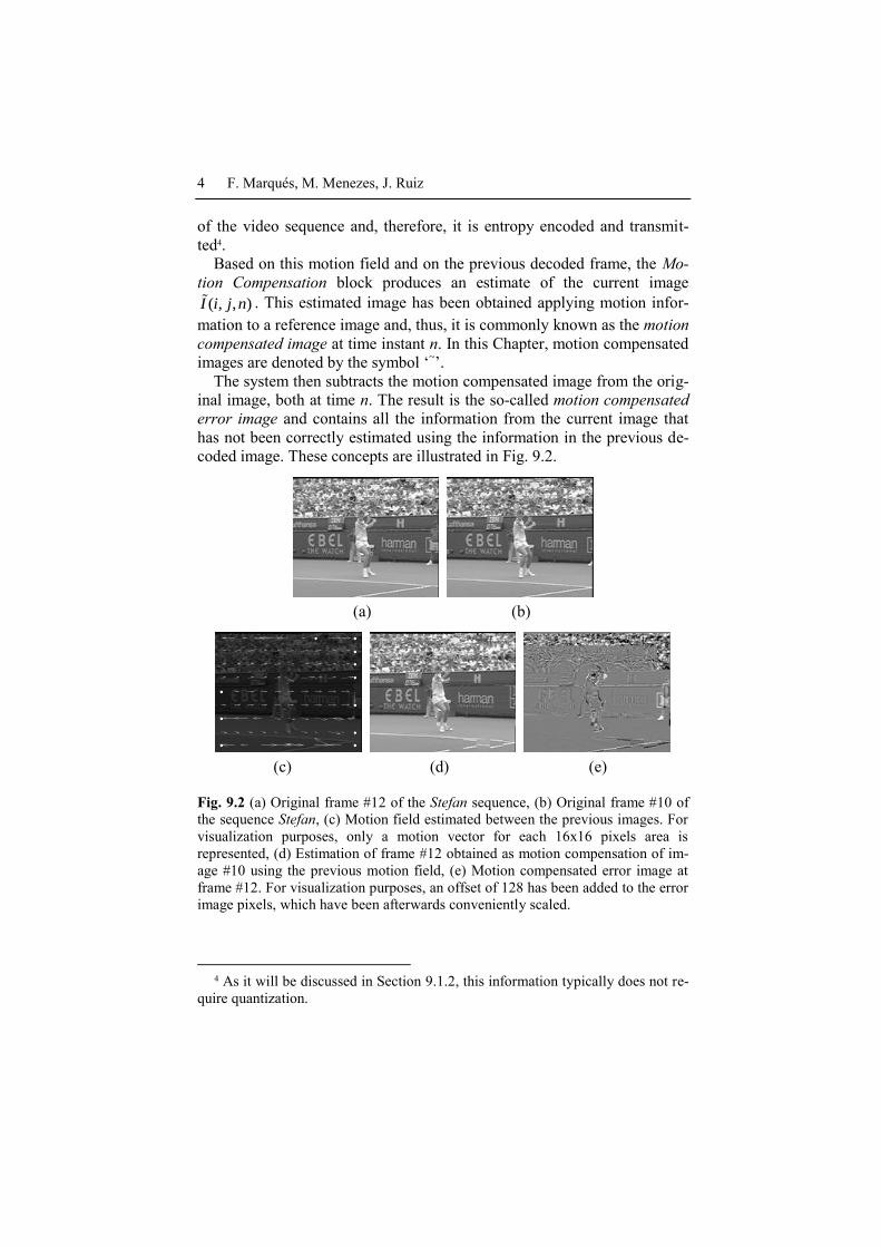
Fig. 9.3 presents the block diagram of the decoder associated to the pre-
vious compression system. As it can be seen, previously decoded images
are stored in the Frame Storage. They will be motion compensated using
the motion information that is transmitted when coding future frames. Now
it is even clearer the usefulness of recovering the decoded images in the
encoder. If it was not the case, the encoder and the decoder would use dif-
ferent information in the motion compensation process. That is, the encod-
er would estimate the motion information using original data whereas the
decoder will apply this motion information on decoded data, leading to dif-
ferent motion compensated images and motion compensated error images.
Fig. 9.3 Decoder system associated to the encoder of Fig. 9.1.
5 Such a system is commonly referred to as a close loop coder-decoder (codec).
6 F. Marqués, M. Menezes, J. Ruiz
9.1.1 Motion estimation: The Block Matching algorithm
In the initial part of this Section, it has been made clear that a paramount
step in video coding is motion estimation (and compensation). There exist
a myriad of motion estimation algorithms (some of them are presented in
Tekalp 1995, Fleet and Wiess 2006) which present different performance
in terms of accuracy of the motion field, computational load, compactness
of the motion representation, etc. Nevertheless, the so-called Block Match-
ing algorithm has been shown to globally outperform all other approaches
in the coding context.
Most motion estimation algorithms rely on the hypothesis that, between
two consecutive (close enough) images, changes are only due to motion
and, therefore, every pixel in the current image I(r, n) has an associated
pixel (a referent) in the reference image I(r, n-1):
( , ) ( ( ), 1)I n I n r r D r (9.1)
where vector r represents the pixel location (x, y) and D(r) the motion field
(also known as optical flow):
( ) [ ( ), ( )]x yd dD r r r (9.2)
The hypothesis in Eq. (9.1) is too restrictive since factors other than mo-
tion influence the variations in the image values between even consecutive
images; typically, changes in the scene illumination, camera noise, reflect-
ing properties of object surfaces, etc. Therefore, motion estimation algo-
rithms do not try to obtain a motion field fulfilling Eq. (9.1). The common
strategy is to compute the so-called Displaced Frame Difference (DFD)
( , ( )) ( , ) ( ( ), 1)DFD I n I n r D r r r D r (9.3)
to define a given metric M{.} over this image and to obtain the motion
field that minimizes this metric:
*
( )
( ) arg min ( , ( ))M DFDD r
D r r D r (9.4)
Note that the image that is subtracted to the current image in Eq. (9.3) is
obtained by applying the estimated motion vectors D(r) to the pixels of the
How are digital TV programs compressed to allow broadcasting? 7
reference image. This is what, in the context of video coding, we have
called motion compensated image:
( , ) ( ( ), 1)I n I n r r D r (9.5)
Consequently, the DFD is nothing but the motion compensation error im-
age and the minimization process expressed in Eq. (9.4) looks for the mi-
nimization of a metric defined over an estimation error. Therefore, a typi-
cal choice for the selection of that metric is the energy of the error6:
2*
( )
( ) arg min ( , ( ))R
DFD
D r r
D r r D r (9.6)
where R is, originally, the region of support of the image.
So far, we have not imposed any constraints on the motion vector field
and all its components are independent. This pixel independency is neither
natural, because neighbor pixels are likely to present similar motion, nor
useful in the coding context, because it leads to a different displacement
vector for every pixel, which results into a too large amount of information
to be coded.
Parametric vector fields impose a given motion model to a specific set
of pixels in the image. Common motion models are translational, affine,
linear projective or quadratic. If we assume that the whole image under-
goes the same motion model, the whole motion vector field can be parame-
terized D(r, p), where p is the vector containing the parameters of the
model, and the DFD definition depends now on these parameters p:
( , ) ( , ) ( ( , ), 1)DFD I n I n r p r r D r p (9.7)
The minimization process of Eq. (9.6) aims now at obtaining the optimum
set of parameters:
2*( , ) arg min ( , )
R
DFD
p r
D r p r p (9.8)
6 Although this is a useful choice when theoretical deriving the algorithms,
when actually implementing them, the square error (L2 norm) is commonly re-
placed by the absolute error (the L1 norm) given its lower computational load.
8 F. Marqués, M. Menezes, J. Ruiz
The perfect situation would be to have a parametric motion model as-
signed to every different object in the scene. This solution requires the
segmentation of the scene into its motion homogeneous parts. However,
motion based image segmentation is a very complicated task (segmenta-
tion is often named an ill-posed problem). Moreover, if the image is seg-
mented, the use of the partition for coding purposes would require trans-
mitting the shapes of the arbitrary regions and this boundary information is
extremely difficult to compress.
The adopted solution in video coding is to partition the image into a set
of square blocks (usually referred to as macroblocks) and to estimate the
motion separately within each one of these macroblocks. Therefore, a
fixed partition is used which is known beforehand by the receiver and does
not require to be transmitted. Since this partition is independent of the im-
age contents, data contained in each macroblock may not share the same
motion. However, given the typical macroblock size (e.g.: 16x16 pixels),
motion information within a macroblock can be considered close to homo-
genous. Furthermore, the imposed motion model is translational; that is, all
pixels in a macroblock are assumed to undergo the same motion which, for
each macroblock, is represented by a single displacement vector.
As it has been previously said, the motion (displacement) of every ma-
croblock is separately determined. Therefore, the global minimization
problem is divided into a set of local minimization ones where, for the ith
macroblock MBi, the optimum parameters pi* = [dx*, dy*]i are obtained:
2* * *, arg min ( , )
i
x y iMB
d d DFD
ip r
p r p (9.9)
The common implementation of this minimization process is the so-
called Block Matching algorithm. In the Block Matching, a direct explora-
tion of the solution space is performed. In our case, the solution space is
the space containing all possible macroblock displacements. This way, for
each macroblock in the current image, a search area is defined in the ref-
erence image. The macroblock is placed at various positions within the
search area in the reference image. Those positions are defined by the
search strategy and the quantization step and every position corresponds
to a possible displacement; that is, a point in the solution space. At each
position, the pixel values overlapped by the displaced macroblock are
compared (matched) with the original macroblock pixel values. The way to
perform this comparison is defined by the selected metric. The vector
representing the displacement leading to the best match (lowest metric
value) is the motion vector assigned to this macroblock. The final result of
How are digital TV programs compressed to allow broadcasting? 9
the Block Matching algorithm is a set of displacements (motion vectors),
each one associated to a different macroblock of the current image.
Therefore, several aspects have to be fixed in a concrete implementation
of the Block Matching; namely7:
the metric that defines the best match, while the square error is the
optimum metric in case of assessing the results in terms of PSNR
(see Chapter 8), it is common to implement the absolute error given
its lower computational complexity;
the search area in the reference image, which is related to the max-
imum allowed displacement, that is, to the maximum allowed speed
of objects in the scene (see Section 9.2.2);
the quantization step to represent the parameters of the motion mod-
el, in our case the coordinates of the displacement, which is related
to the accuracy of the motion representation;
the search strategy in the parameter space, which defines which
possible solutions (that is, different displacements) are analyzed in
order to select the motion vector.
The size of the search area is application dependent. For example, it is
clear that the maximum displacement expected by objects in the scene is
very different for a sport video than for an interview program. A possible
simplification is to fix the maximum displacement in any direction close to
the size of a macroblock side. This leads to space solutions covering zones
of, for example, size [-15, 15] x [-15, 15].
The quantization step is related to the precision used to represent the
motion parameters. Objects in the scene do not move in terms of pixels
and, therefore, to describe their motion by means of an integer number of
pixels is to reduce the accuracy of the motion representation. In current
standards, techniques to estimate the motion with a quantization step of ½
and even ¼ of pixel are implemented8. The quantization step samples the
space solution and defines a finite set of possible solutions. For instance, if
we fix the quantization step to 1 pixel, the previous space solution of size
[-15, 15] x [-15, 15] leads to 31x31 = 961 possible solutions; that is, 961
different displacement vectors that have to be tested to find the optimum
one. Note that, if we use a quantization step of 1/N of pixel, we are in-
creasing the number of possible solutions by a factor N2.
7 We could add here other aspects such as the macroblock shape and size but, as
previously commented, we are assuming in the whole Chapter that square macrob-
locks of size 16x16 pixels are used. 8 Sub-pixel accuracy requires interpolation of the reference image. This kind of
techniques, although very much used in current standards mainly to reach high
quality decoded images, is out of the scope of this Chapter.
10 F. Marqués, M. Menezes, J. Ruiz
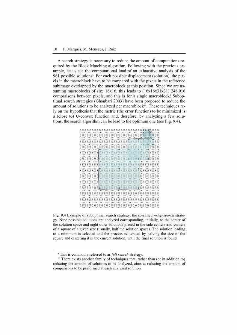
A search strategy is necessary to reduce the amount of computations re-
quired by the Block Matching algorithm. Following with the previous ex-
ample, let us see the computational load of an exhaustive analysis of the
961 possible solutions9. For each possible displacement (solution), the pix-
els in the macroblock have to be compared with the pixels in the reference
subimage overlapped by the macroblock at this position. Since we are as-
suming macroblocks of size 16x16, this leads to (16x16x31x31) 246.016
comparisons between pixels, and this is for a single macroblock! Subop-
timal search strategies (Ghanbari 2003) have been proposed to reduce the
amount of solutions to be analyzed per macroblock10. These techniques re-
ly on the hypothesis that the metric (the error function) to be minimized is
a (close to) U-convex function and, therefore, by analyzing a few solu-
tions, the search algorithm can be lead to the optimum one (see Fig. 9.4).
Fig. 9.4 Example of suboptimal search strategy: the so-called nstep-search strate-
gy. Nine possible solutions are analyzed corresponding, initially, to the center of
the solution space and eight other solutions placed in the side centers and corners
of a square of a given size (usually, half the solution space). The solution leading
to a minimum is selected and the process is iterated by halving the size of the
square and centering it in the current solution, until the final solution is found.
9 This is commonly referred to as full search strategy. 10 There exists another family of techniques that, rather than (or in addition to)
reducing the amount of solutions to be analyzed, aims at reducing the amount of
comparisons to be performed at each analyzed solution.
How are digital TV programs compressed to allow broadcasting? 11
9.1.2 A few specificities of video coding standards
The complexity of current video standards is extremely high, incorporating
a large variety of techniques for decorrelating the information and allow-
ing the selection of one technique or another at, even, the sub-block level
(see, for instance, Sullivan and Wiegand 2005). Analyzing all these possi-
bilities is out of the scope of this Chapter and, instead, we are going to
concentrate on a few additional concepts that (i) are basically shared by all
video standards, (ii) complete the description of a simple video codec and
(iii) help understanding the potential of the motion estimation process.
This way, we present the three different types of frames that are defined
and the concept of Group of Pictures (GOP), we discuss how the motion
information is decorrelated and entropy coded and, finally, we comment
on the main variations that the specific nature of the motion compensated
error image introduces in its coding.
I-Pictures, P-Pictures and B-Pictures
The use of motion information to perform temporal prediction improves
the compression efficiency as it will be shown in Section 9.2. However,
coding standards are not only required to achieve high compression effi-
ciency but to fulfill other functionalities as well. Among these additional
features, a basic one is random access. Random access is defined as “the
process of beginning to read and decode the coded bitstream at an arbitrary
point” (MPEG 1993). Actually, random access requires that any picture
can be decoded in a limited amount of time, which is an essential feature
for video on a storage medium11. This requirement implies having a set of
access points in the bitstream, associated to specific images, which are eas-
ily identifiable and can be decoded without reference to previous segments
of the bitstream. The way to implement these requirements is by breaking
the temporal prediction chain and introducing some images encoded in in-
tra mode, the so-called Intra-Pictures or I-Pictures. The spacing of two I-
Pictures per second depends on the application. Applications requiring
random access may demand short spacing, which can be achieve without
significant loss of compression rate. Other applications may even use I-
Pictures to improve the compression where motion compensation reveals
ineffective; for instance, in a scene cut. Nevertheless, since I-Pictures will
be used as reference for future frames in the sequence, they are coded with
good quality; that is, with moderate compression.
11 Think, for example, about the functionalities of fast forward and fast reverse
playback that we commonly use in a DVD player.
12 F. Marqués, M. Menezes, J. Ruiz
Relying on I-Pictures, new images can be temporally predicted and en-
coded. This is the case of Predictive coded pictures (P-Pictures), which are
coded more efficiently, using as reference image a previous I-Picture or P-
Picture, commonly, the nearest one. Note that P-Pictures are used as refer-
ence for further prediction and, therefore, their quality has to be high
enough for that purpose.
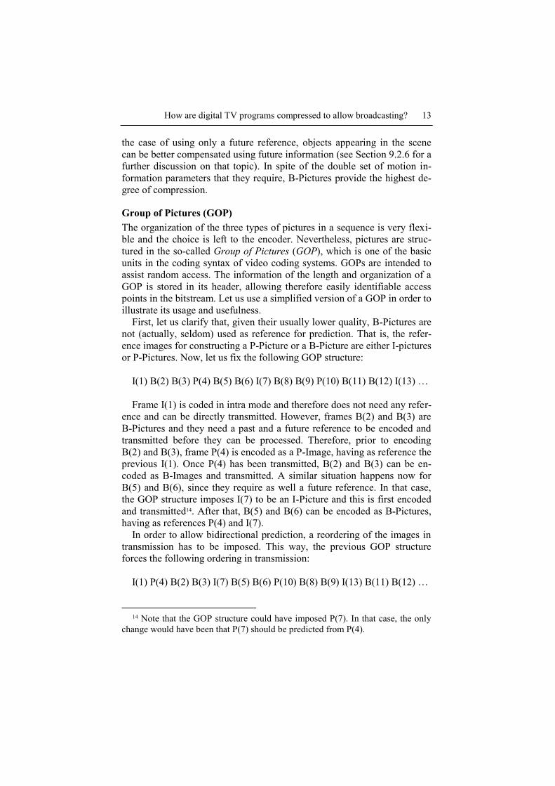
Finally, a third type of images is defined in usual video coding systems,
which are the so-called Bidirectionally-predictive coded pictures (B-
Pictures). B-Pictures are estimated combining the information of two ref-
erence images, one preceding it and the other following it in the video se-
quence (see Fig. 9.5). Therefore, B-Pictures use both past and future refer-
ence pictures for motion compensation12. The combination of past and
future information has several implications.
Fig. 9.5 Illustration of the motion prediction in B-Pictures.
First, in order to allow using future frames as references, the image
transmission order has to be different from the displaying order. This con-
cept will be further discussed in the sequel. Second, B-Pictures may use
past, future or combinations of both images in their prediction. In the case
of combining both references, the selected subimages in the past and future
reference images are linearly combined to produce the motion compen-
sated estimation13. This selection of references leads to an increase in mo-
tion compensation efficiency. In the case of combining past and future ref-
erences, the linear combination may imply a noise reduction. Moreover, in
12 Commonly, estimation from past references is named forward prediction
whereas estimation from future references is named backward prediction. 13 Linear weights are inversely proportional to the distance between the B-
Picture and the reference image.
How are digital TV programs compressed to allow broadcasting? 13
the case of using only a future reference, objects appearing in the scene
can be better compensated using future information (see Section 9.2.6 for a
further discussion on that topic). In spite of the double set of motion in-
formation parameters that they require, B-Pictures provide the highest de-
gree of compression.
Group of Pictures (GOP)
The organization of the three types of pictures in a sequence is very flexi-
ble and the choice is left to the encoder. Nevertheless, pictures are struc-
tured in the so-called Group of Pictures (GOP), which is one of the basic
units in the coding syntax of video coding systems. GOPs are intended to
assist random access. The information of the length and organization of a
GOP is stored in its header, allowing therefore easily identifiable access
points in the bitstream. Let us use a simplified version of a GOP in order to
illustrate its usage and usefulness.
First, let us clarify that, given their usually lower quality, B-Pictures are
not (actually, seldom) used as reference for prediction. That is, the refer-
ence images for constructing a P-Picture or a B-Picture are either I-pictures
or P-Pictures. Now, let us fix the following GOP structure:
I(1) B(2) B(3) P(4) B(5) B(6) I(7) B(8) B(9) P(10) B(11) B(12) I(13) …
Frame I(1) is coded in intra mode and therefore does not need any refer-
ence and can be directly transmitted. However, frames B(2) and B(3) are
B-Pictures and they need a past and a future reference to be encoded and
transmitted before they can be processed. Therefore, prior to encoding
B(2) and B(3), frame P(4) is encoded as a P-Image, having as reference the
previous I(1). Once P(4) has been transmitted, B(2) and B(3) can be en-
coded as B-Images and transmitted. A similar situation happens now for
B(5) and B(6), since they require as well a future reference. In that case,
the GOP structure imposes I(7) to be an I-Picture and this is first encoded
and transmitted14. After that, B(5) and B(6) can be encoded as B-Pictures,
having as references P(4) and I(7).
In order to allow bidirectional prediction, a reordering of the images in
transmission has to be imposed. This way, the previous GOP structure
forces the following ordering in transmission:
I(1) P(4) B(2) B(3) I(7) B(5) B(6) P(10) B(8) B(9) I(13) B(11) B(12) …
14 Note that the GOP structure could have imposed P(7). In that case, the only
change would have been that P(7) should be predicted from P(4).
14 F. Marqués, M. Menezes, J. Ruiz
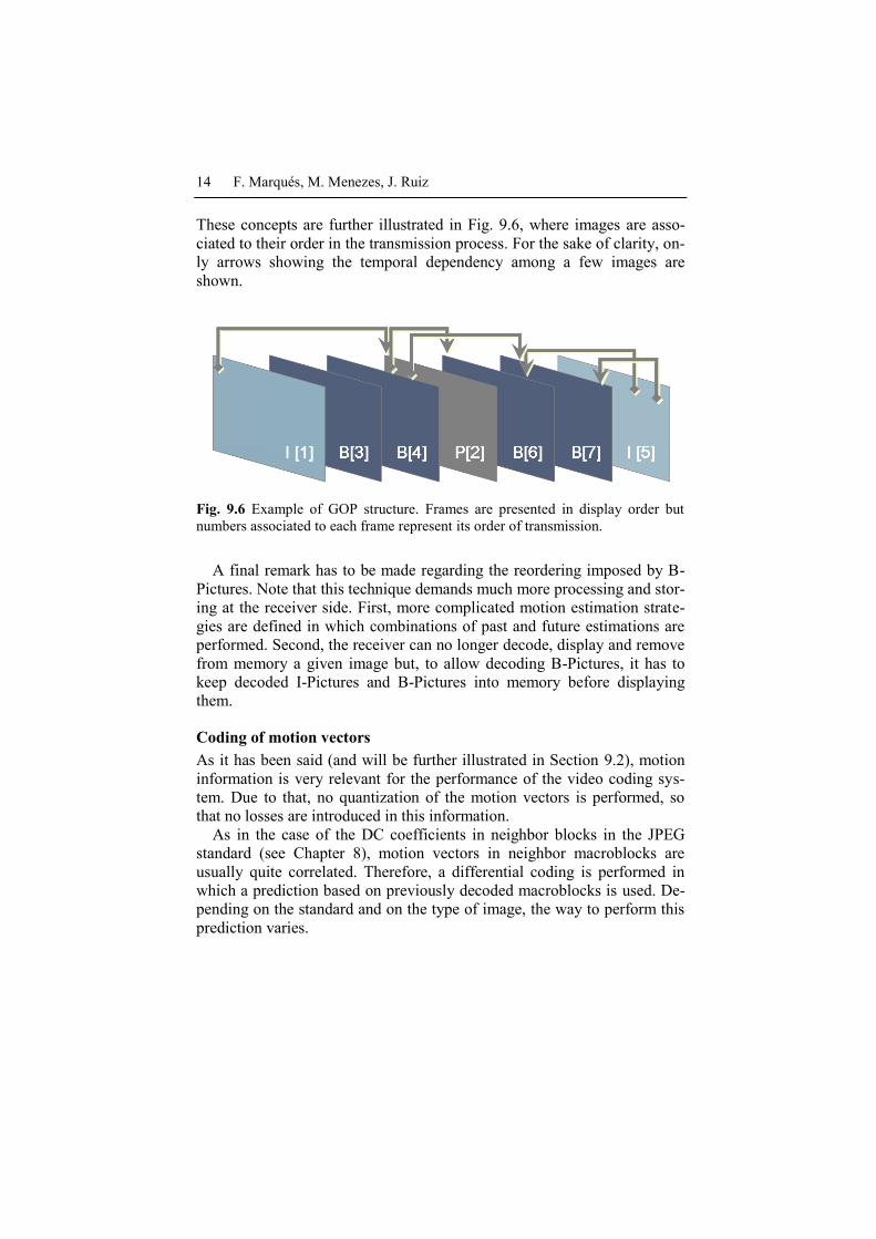
These concepts are further illustrated in Fig. 9.6, where images are asso-
ciated to their order in the transmission process. For the sake of clarity, on-
ly arrows showing the temporal dependency among a few images are
shown.
Fig. 9.6 Example of GOP structure. Frames are presented in display order but
numbers associated to each frame represent its order of transmission.
A final remark has to be made regarding the reordering imposed by B-
Pictures. Note that this technique demands much more processing and stor-
ing at the receiver side. First, more complicated motion estimation strate-
gies are defined in which combinations of past and future estimations are
performed. Second, the receiver can no longer decode, display and remove
from memory a given image but, to allow decoding B-Pictures, it has to
keep decoded I-Pictures and B-Pictures into memory before displaying
them.
Coding of motion vectors
As it has been said (and will be further illustrated in Section 9.2), motion
information is very relevant for the performance of the video coding sys-
tem. Due to that, no quantization of the motion vectors is performed, so
that no losses are introduced in this information.
As in the case of the DC coefficients in neighbor blocks in the JPEG
standard (see Chapter 8), motion vectors in neighbor macroblocks are
usually quite correlated. Therefore, a differential coding is performed in
which a prediction based on previously decoded macroblocks is used. De-
pending on the standard and on the type of image, the way to perform this
prediction varies.
How are digital TV programs compressed to allow broadcasting? 15
DCT coefficient quantization of the motion compensated error image
When presenting the procedure for quantizing the DCT coefficients in still
image coding (see Chapter 8), it was commented that a specific quantiza-
tion table was used to take into account the different relevance of each
coefficient for the human visual system. It that case, the study of the hu-
man visual system lead to the use of the so-called Lohscheller tables that,
roughly speaking, impose a stronger quantization step to higher frequency
coefficients.
In the case of coding the motion compensated error image, this strategy
is no longer useful. Note that the presence of high frequency components
in the error image may not be related to high frequency information in the
original image but, very likely, to poor motion compensation. Therefore, a
flat default matrix is commonly used (all matrix components set to 16).
9.2 MATLAB proof of concept
In the following Section we are going to illustrate the main concepts be-
hind compression of image sequences. Image sequences present temporal
as well as spatial redundancy. In order to correctly exploit the temporal re-
dundancy between temporally neighbor images, the motion present in the
scene has to be estimated. Once the motion is estimated, the information in
the image used as reference is motion compensated to produce a first esti-
mation of the image to be coded. Motion estimation is performed by divid-
ing the image into non-overlapping square blocks and estimating the mo-
tion of each block independently.
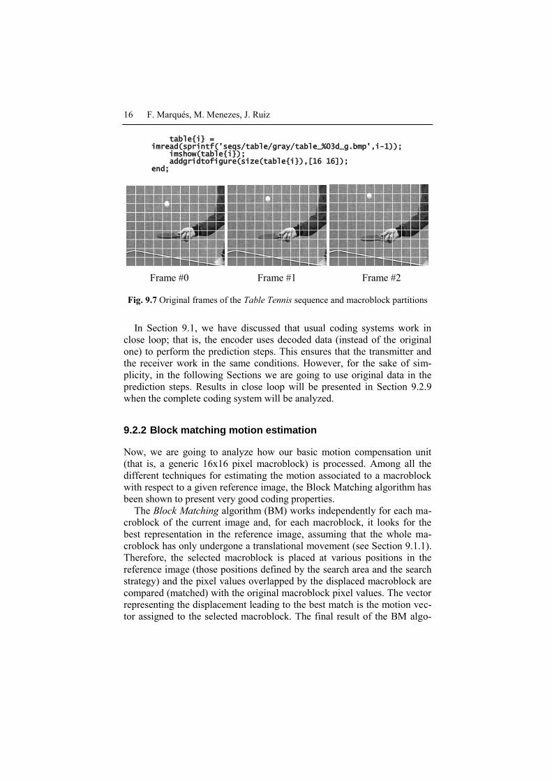
9.2.1 Macroblock processing
Typically, for motion estimation, images are partitioned into blocks of
16x16 pixels15, which will be referred to as macroblocks (see Fig. 9.7). The
macroblock partition is hierarchical with respect to the block partition (see
Chapter 8) and, therefore, every macroblock contains 4 blocks. As in the
block case, images are padded to allow an exact partition in terms of ma-
croblocks.
for i=1:3,
15 Current standards allow finer partitions using both smaller square blocks
(e.g.: 8x8) and smaller rectangular blocks (e.g.: 16x8, 8x16, etc.)
16 F. Marqués, M. Menezes, J. Ruiz
table{i} = imread(sprintf('seqs/table/gray/table_%03d_g.bmp',i-1)); imshow(table{i}); addgridtofigure(size(table{i}),[16 16]); end;
Frame #0 Frame #1 Frame #2
Fig. 9.7 Original frames of the Table Tennis sequence and macroblock partitions
In Section 9.1, we have discussed that usual coding systems work in
close loop; that is, the encoder uses decoded data (instead of the original
one) to perform the prediction steps. This ensures that the transmitter and
the receiver work in the same conditions. However, for the sake of sim-
plicity, in the following Sections we are going to use original data in the
prediction steps. Results in close loop will be presented in Section 9.2.9
when the complete coding system will be analyzed.
9.2.2 Block matching motion estimation
Now, we are going to analyze how our basic motion compensation unit
(that is, a generic 16x16 pixel macroblock) is processed. Among all the
different techniques for estimating the motion associated to a macroblock
with respect to a given reference image, the Block Matching algorithm has
been shown to present very good coding properties.
The Block Matching algorithm (BM) works independently for each ma-
croblock of the current image and, for each macroblock, it looks for the
best representation in the reference image, assuming that the whole ma-
croblock has only undergone a translational movement (see Section 9.1.1).
Therefore, the selected macroblock is placed at various positions in the
reference image (those positions defined by the search area and the search
strategy) and the pixel values overlapped by the displaced macroblock are
compared (matched) with the original macroblock pixel values. The vector
representing the displacement leading to the best match is the motion vec-
tor assigned to the selected macroblock. The final result of the BM algo-
How are digital TV programs compressed to allow broadcasting? 17
rithm is a set of displacements (motion vectors), each one associated to a
different macroblock of the current image.
As commented in the Section 9.1.1, several aspects have to be fixed in a
concrete implementation of the BM; namely: (i) the metric that defines the
best match; (ii) the search area in the reference image, which is related to
the maximum allowed speed of objects in the scene; (iii) the quantization
step to represent the coordinates of the motion vector, which is related to
the accuracy of the motion representation; and (iv) the search strategy in
the parameter space, which defines how many possible solutions (that is,
different displacements) are analyzed in order to select the motion vector.
The MATLAB function estimatemotion performs the BM of a given
image with respect to a reference image. In it, the previous aspects are im-
plemented as follows: (i) the selected metric is the absolute difference; (ii)
the search area can be set by the fourth parameter (actually, this parameter
does not directly set the search area but the maximum displacement al-
lowed to the motion vector, so a value of [16 12] indicates that the motion
vector can have values from (-16,-12) to (16,12)); (iii) the quantization
step has been set to 1 pixel; and (iv) as search strategy both a full search
and an nstep-search (see Fig. 9.4) within the search area are implemented.
t = 2; [mvv mvh] = estimatemotion(table{t},table{t-1},[16 16],... [15 15],'fullsearch');
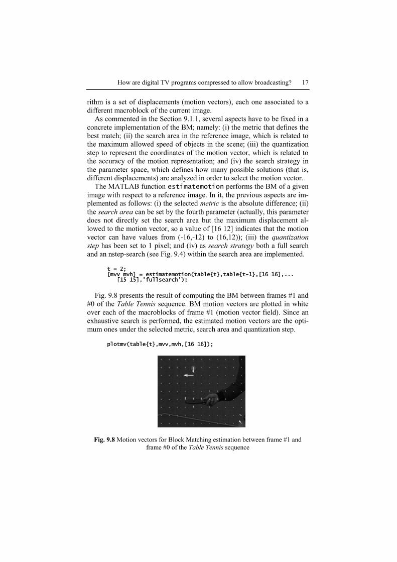
Fig. 9.8 presents the result of computing the BM between frames #1 and
#0 of the Table Tennis sequence. BM motion vectors are plotted in white
over each of the macroblocks of frame #1 (motion vector field). Since an
exhaustive search is performed, the estimated motion vectors are the opti-
mum ones under the selected metric, search area and quantization step.
plotmv(table{t},mvv,mvh,[16 16]);
Fig. 9.8 Motion vectors for Block Matching estimation between frame #1 and
frame #0 of the Table Tennis sequence
18 F. Marqués, M. Menezes, J. Ruiz
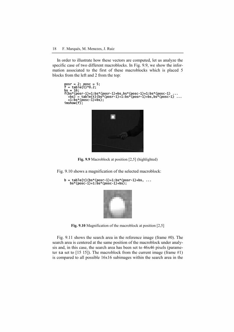
In order to illustrate how these vectors are computed, let us analyze the
specific case of two different macroblocks. In Fig. 9.9, we show the infor-
mation associated to the first of these macroblocks which is placed 5
blocks from the left and 2 from the top:
posr = 2; posc = 5; f = table{t}*0.2; bs = 16; f(bs*(posr-1)+1:bs*(posr-1)+bs,bs*(posc-1)+1:bs*(posc-1) ... +bs) = table{t}(bs*(posr-1)+1:bs*(posr-1)+bs,bs*(posc-1) ... +1:bs*(posc-1)+bs); imshow(f);
Fig. 9.9 Macroblock at position [2,5] (highlighted)
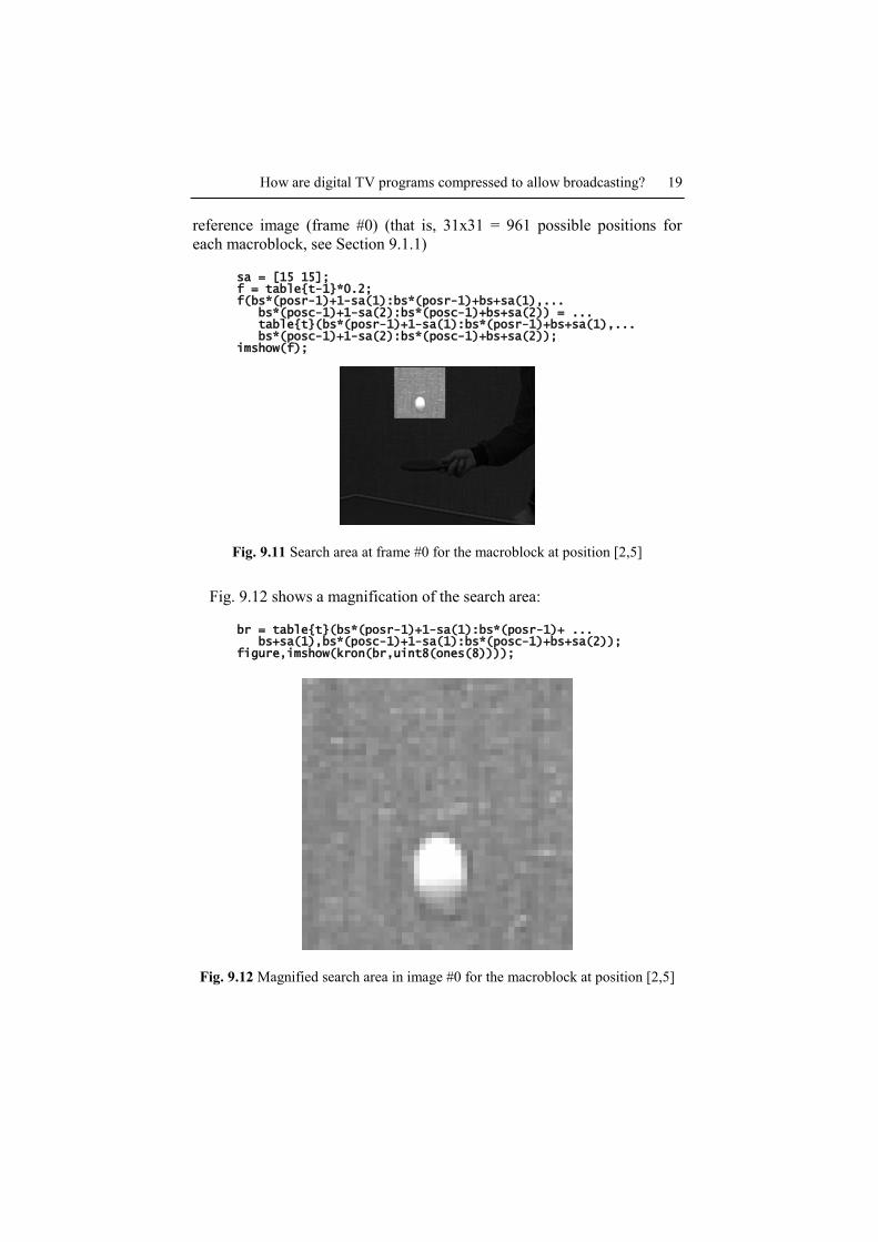
Fig. 9.10 shows a magnification of the selected macroblock:
b = table{t}(bs*(posr-1)+1:bs*(posr-1)+bs, ... bs*(posc-1)+1:bs*(posc-1)+bs);
Fig. 9.10 Magnification of the macroblock at position [2,5]
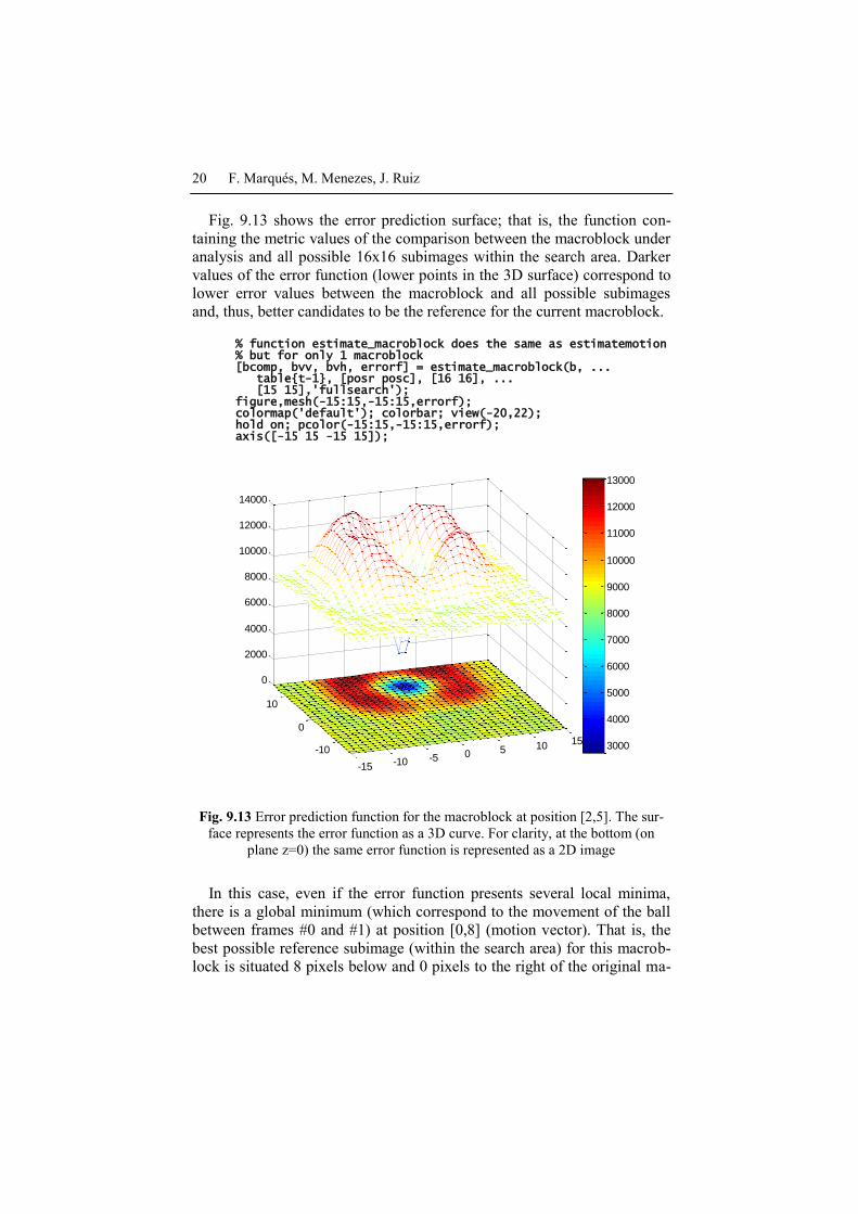
Fig. 9.11 shows the search area in the reference image (frame #0). The
search area is centered at the same position of the macroblock under analy-
sis and, in this case, the search area has been set to 46x46 pixels (parame-
ter sa set to [15 15]). The macroblock from the current image (frame #1)
is compared to all possible 16x16 subimages within the search area in the
How are digital TV programs compressed to allow broadcasting? 19
reference image (frame #0) (that is, 31x31 = 961 possible positions for
each macroblock, see Section 9.1.1)
sa = [15 15]; f = table{t-1}*0.2; f(bs*(posr-1)+1-sa(1):bs*(posr-1)+bs+sa(1),... bs*(posc-1)+1-sa(2):bs*(posc-1)+bs+sa(2)) = ... table{t}(bs*(posr-1)+1-sa(1):bs*(posr-1)+bs+sa(1),... bs*(posc-1)+1-sa(2):bs*(posc-1)+bs+sa(2)); imshow(f);
Fig. 9.11 Search area at frame #0 for the macroblock at position [2,5]
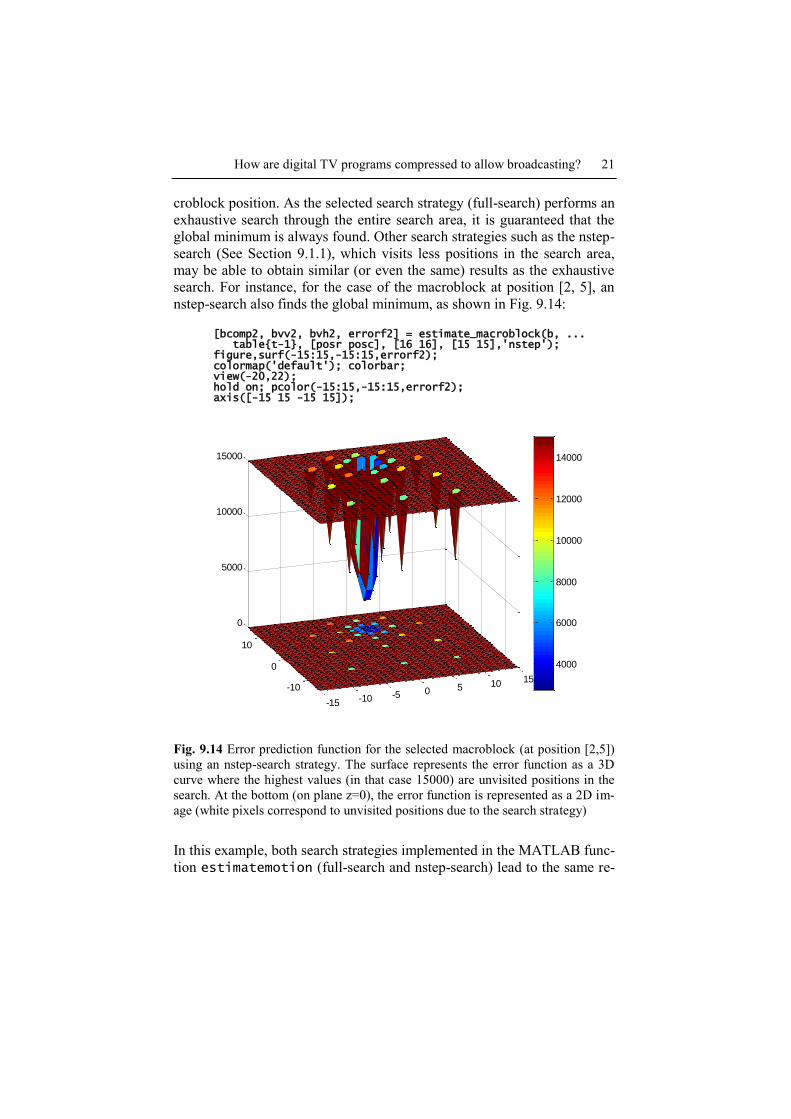
Fig. 9.12 shows a magnification of the search area:
br = table{t}(bs*(posr-1)+1-sa(1):bs*(posr-1)+ ... bs+sa(1),bs*(posc-1)+1-sa(1):bs*(posc-1)+bs+sa(2)); figure,imshow(kron(br,uint8(ones(8))));
Fig. 9.12 Magnified search area in image #0 for the macroblock at position [2,5]
20 F. Marqués, M. Menezes, J. Ruiz
Fig. 9.13 shows the error prediction surface; that is, the function con-
taining the metric values of the comparison between the macroblock under
analysis and all possible 16x16 subimages within the search area. Darker
values of the error function (lower points in the 3D surface) correspond to
lower error values between the macroblock and all possible subimages
and, thus, better candidates to be the reference for the current macroblock.
% function estimate_macroblock does the same as estimatemotion % but for only 1 macroblock [bcomp, bvv, bvh, errorf] = estimate_macroblock(b, ... table{t-1}, [posr posc], [16 16], ... [15 15],'fullsearch'); figure,mesh(-15:15,-15:15,errorf); colormap('default'); colorbar; view(-20,22); hold on; pcolor(-15:15,-15:15,errorf); axis([-15 15 -15 15]);
-15 -10 -5 0 5 10 15-10
0
10
0
2000
4000
6000
8000
10000
12000
14000
3000
4000
5000
6000
7000
8000
9000
10000
11000
12000
13000
Fig. 9.13 Error prediction function for the macroblock at position [2,5]. The sur-
face represents the error function as a 3D curve. For clarity, at the bottom (on
plane z=0) the same error function is represented as a 2D image
In this case, even if the error function presents several local minima,
there is a global minimum (which correspond to the movement of the ball
between frames #0 and #1) at position [0,8] (motion vector). That is, the
best possible reference subimage (within the search area) for this macrob-
lock is situated 8 pixels below and 0 pixels to the right of the original ma-
How are digital TV programs compressed to allow broadcasting? 21
croblock position. As the selected search strategy (full-search) performs an
exhaustive search through the entire search area, it is guaranteed that the
global minimum is always found. Other search strategies such as the nstep-
search (See Section 9.1.1), which visits less positions in the search area,
may be able to obtain similar (or even the same) results as the exhaustive
search. For instance, for the case of the macroblock at position [2, 5], an
nstep-search also finds the global minimum, as shown in Fig. 9.14:
[bcomp2, bvv2, bvh2, errorf2] = estimate_macroblock(b, ... table{t-1}, [posr posc], [16 16], [15 15],'nstep'); figure,surf(-15:15,-15:15,errorf2); colormap('default'); colorbar; view(-20,22); hold on; pcolor(-15:15,-15:15,errorf2); axis([-15 15 -15 15]);
-15 -10 -5 0 5 10 15-10
0
10
0
5000
10000
15000
4000
6000
8000
10000
12000
14000
Fig. 9.14 Error prediction function for the selected macroblock (at position [2,5])
using an nstep-search strategy. The surface represents the error function as a 3D
curve where the highest values (in that case 15000) are unvisited positions in the
search. At the bottom (on plane z=0), the error function is represented as a 2D im-
age (white pixels correspond to unvisited positions due to the search strategy)
In this example, both search strategies implemented in the MATLAB func-
tion estimatemotion (full-search and nstep-search) lead to the same re-
22 F. Marqués, M. Menezes, J. Ruiz
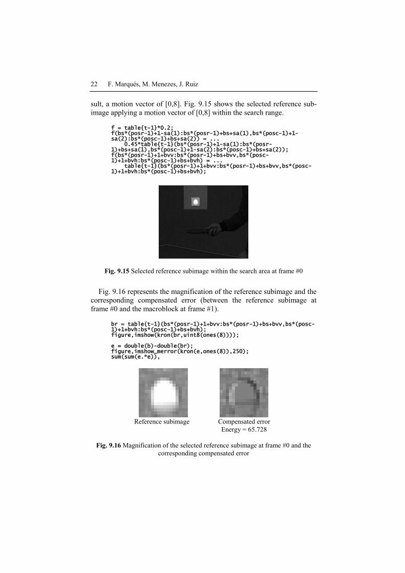
sult, a motion vector of [0,8]. Fig. 9.15 shows the selected reference sub-
image applying a motion vector of [0,8] within the search range.
f = table{t-1}*0.2; f(bs*(posr-1)+1-sa(1):bs*(posr-1)+bs+sa(1),bs*(posc-1)+1-sa(2):bs*(posc-1)+bs+sa(2)) = ... 0.45*table{t-1}(bs*(posr-1)+1-sa(1):bs*(posr-1)+bs+sa(1),bs*(posc-1)+1-sa(2):bs*(posc-1)+bs+sa(2)); f(bs*(posr-1)+1+bvv:bs*(posr-1)+bs+bvv,bs*(posc-1)+1+bvh:bs*(posc-1)+bs+bvh) = ... table{t-1}(bs*(posr-1)+1+bvv:bs*(posr-1)+bs+bvv,bs*(posc-1)+1+bvh:bs*(posc-1)+bs+bvh);
Fig. 9.15 Selected reference subimage within the search area at frame #0
Fig. 9.16 represents the magnification of the reference subimage and the
corresponding compensated error (between the reference subimage at
frame #0 and the macroblock at frame #1).
br = table{t-1}(bs*(posr-1)+1+bvv:bs*(posr-1)+bs+bvv,bs*(posc-1)+1+bvh:bs*(posc-1)+bs+bvh); figure,imshow(kron(br,uint8(ones(8))));
e = double(b)-double(br); figure,imshow_merror(kron(e,ones(8)),250); sum(sum(e.*e)),
Reference subimage Compensated error
Energy = 65.728
Fig. 9.16 Magnification of the selected reference subimage at frame #0 and the
corresponding compensated error
How are digital TV programs compressed to allow broadcasting? 23
Through this Chapter, in order to present error images, an offset of 128
is added to all pixel values and, if necessary, they are clipped to the [0,
255] range. This way, zero error is represented by a 128 value
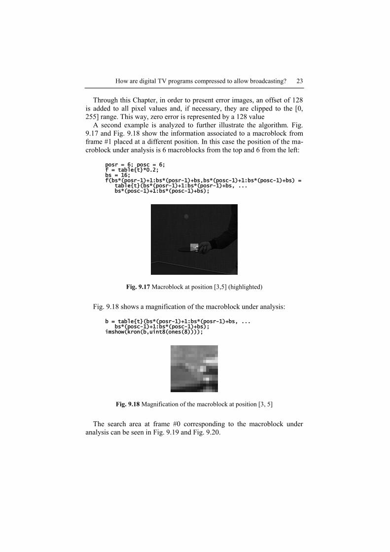
A second example is analyzed to further illustrate the algorithm. Fig.
9.17 and Fig. 9.18 show the information associated to a macroblock from
frame #1 placed at a different position. In this case the position of the ma-
croblock under analysis is 6 macroblocks from the top and 6 from the left:
posr = 6; posc = 6; f = table{t}*0.2; bs = 16; f(bs*(posr-1)+1:bs*(posr-1)+bs,bs*(posc-1)+1:bs*(posc-1)+bs) = table{t}(bs*(posr-1)+1:bs*(posr-1)+bs, ... bs*(posc-1)+1:bs*(posc-1)+bs);
Fig. 9.17 Macroblock at position [3,5] (highlighted)
Fig. 9.18 shows a magnification of the macroblock under analysis:
b = table{t}(bs*(posr-1)+1:bs*(posr-1)+bs, ... bs*(posc-1)+1:bs*(posc-1)+bs); imshow(kron(b,uint8(ones(8))));
Fig. 9.18 Magnification of the macroblock at position [3, 5]
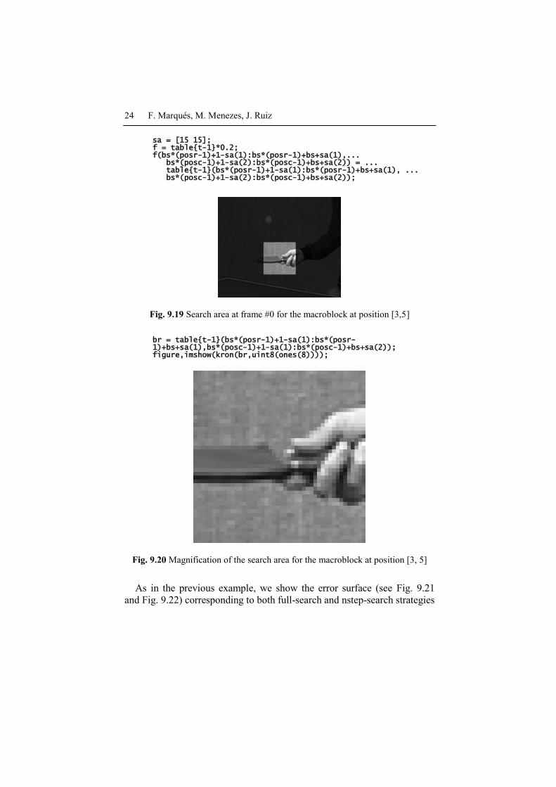
The search area at frame #0 corresponding to the macroblock under
analysis can be seen in Fig. 9.19 and Fig. 9.20.
24 F. Marqués, M. Menezes, J. Ruiz
sa = [15 15]; f = table{t-1}*0.2; f(bs*(posr-1)+1-sa(1):bs*(posr-1)+bs+sa(1),... bs*(posc-1)+1-sa(2):bs*(posc-1)+bs+sa(2)) = ... table{t-1}(bs*(posr-1)+1-sa(1):bs*(posr-1)+bs+sa(1), ... bs*(posc-1)+1-sa(2):bs*(posc-1)+bs+sa(2));
Fig. 9.19 Search area at frame #0 for the macroblock at position [3,5]
br = table{t-1}(bs*(posr-1)+1-sa(1):bs*(posr-1)+bs+sa(1),bs*(posc-1)+1-sa(1):bs*(posc-1)+bs+sa(2)); figure,imshow(kron(br,uint8(ones(8))));
Fig. 9.20 Magnification of the search area for the macroblock at position [3, 5]
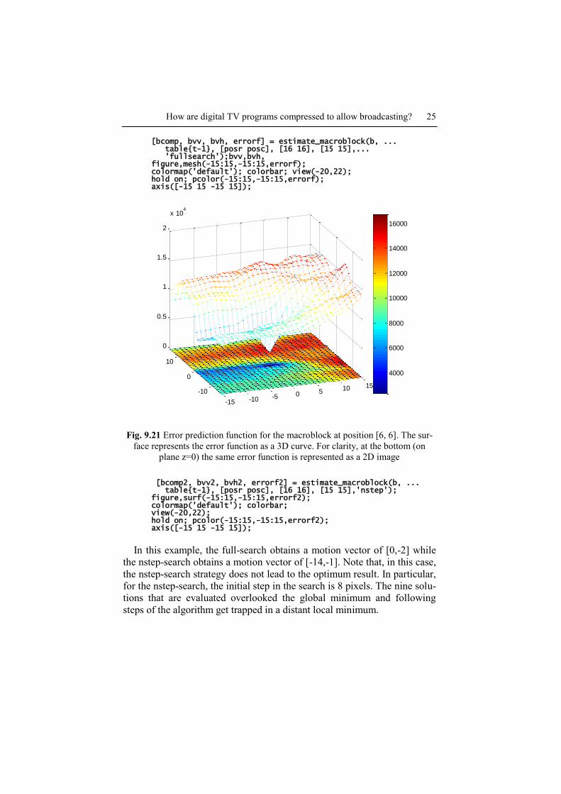
As in the previous example, we show the error surface (see Fig. 9.21
and Fig. 9.22) corresponding to both full-search and nstep-search strategies
How are digital TV programs compressed to allow broadcasting? 25
[bcomp, bvv, bvh, errorf] = estimate_macroblock(b, ... table{t-1}, [posr posc], [16 16], [15 15],... 'fullsearch');bvv,bvh, figure,mesh(-15:15,-15:15,errorf); colormap('default'); colorbar; view(-20,22); hold on; pcolor(-15:15,-15:15,errorf); axis([-15 15 -15 15]);
-15 -10 -5 0 5 10 15-10
0
10
0
0.5
1
1.5
2
x 104
4000
6000
8000
10000
12000
14000
16000
Fig. 9.21 Error prediction function for the macroblock at position [6, 6]. The sur-
face represents the error function as a 3D curve. For clarity, at the bottom (on
plane z=0) the same error function is represented as a 2D image
[bcomp2, bvv2, bvh2, errorf2] = estimate_macroblock(b, ... table{t-1}, [posr posc], [16 16], [15 15],'nstep'); figure,surf(-15:15,-15:15,errorf2); colormap('default'); colorbar; view(-20,22); hold on; pcolor(-15:15,-15:15,errorf2); axis([-15 15 -15 15]);
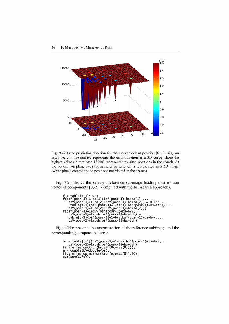
In this example, the full-search obtains a motion vector of [0,-2] while
the nstep-search obtains a motion vector of [-14,-1]. Note that, in this case,
the nstep-search strategy does not lead to the optimum result. In particular,
for the nstep-search, the initial step in the search is 8 pixels. The nine solu-
tions that are evaluated overlooked the global minimum and following
steps of the algorithm get trapped in a distant local minimum.
26 F. Marqués, M. Menezes, J. Ruiz
-15 -10 -5 0 5 10 15-10
0
10
0
5000
10000
15000
0.6
0.7
0.8
0.9
1
1.1
1.2
1.3
1.4
1.5x 10
4
Fig. 9.22 Error prediction function for the macroblock at position [6, 6] using an
nstep-search. The surface represents the error function as a 3D curve where the
highest value (in that case 15000) represents unvisited positions in the search. At
the bottom (on plane z=0) the same error function is represented as a 2D image
(white pixels correspond to positions not visited in the search)
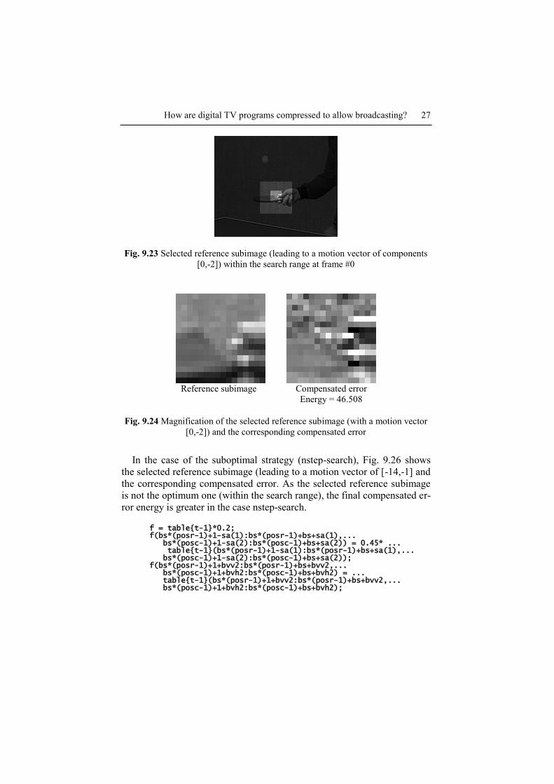
Fig. 9.23 shows the selected reference subimage leading to a motion
vector of components [0,-2] (computed with the full-search approach).
f = table{t-1}*0.2; f(bs*(posr-1)+1-sa(1):bs*(posr-1)+bs+sa(1),... bs*(posc-1)+1-sa(2):bs*(posc-1)+bs+sa(2)) = 0.45* ... table{t-1}(bs*(posr-1)+1-sa(1):bs*(posr-1)+bs+sa(1),... bs*(posc-1)+1-sa(2):bs*(posc-1)+bs+sa(2)); f(bs*(posr-1)+1+bvv:bs*(posr-1)+bs+bvv,... bs*(posc-1)+1+bvh:bs*(posc-1)+bs+bvh) = ... table{t-1}(bs*(posr-1)+1+bvv:bs*(posr-1)+bs+bvv,... bs*(posc-1)+1+bvh:bs*(posc-1)+bs+bvh);
Fig. 9.24 represents the magnification of the reference subimage and the
corresponding compensated error.
br = table{t-1}(bs*(posr-1)+1+bvv:bs*(posr-1)+bs+bvv,... bs*(posc-1)+1+bvh:bs*(posc-1)+bs+bvh); figure,imshow(kron(br,uint8(ones(8)))); e = double(b)-double(br); figure,imshow_merror(kron(e,ones(8)),70); sum(sum(e.*e)),
How are digital TV programs compressed to allow broadcasting? 27
Fig. 9.23 Selected reference subimage (leading to a motion vector of components
[0,-2]) within the search range at frame #0
Reference subimage Compensated error
Energy = 46.508
Fig. 9.24 Magnification of the selected reference subimage (with a motion vector
[0,-2]) and the corresponding compensated error
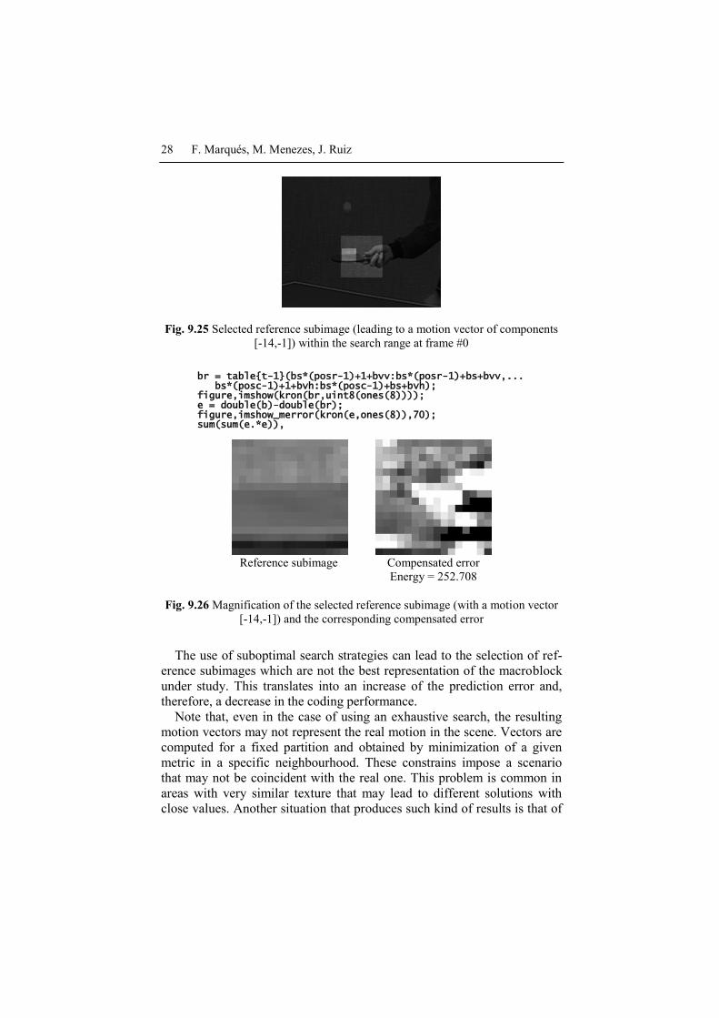
In the case of the suboptimal strategy (nstep-search), Fig. 9.26 shows
the selected reference subimage (leading to a motion vector of [-14,-1] and
the corresponding compensated error. As the selected reference subimage
is not the optimum one (within the search range), the final compensated er-
ror energy is greater in the case nstep-search.
f = table{t-1}*0.2; f(bs*(posr-1)+1-sa(1):bs*(posr-1)+bs+sa(1),... bs*(posc-1)+1-sa(2):bs*(posc-1)+bs+sa(2)) = 0.45* ... table{t-1}(bs*(posr-1)+1-sa(1):bs*(posr-1)+bs+sa(1),... bs*(posc-1)+1-sa(2):bs*(posc-1)+bs+sa(2)); f(bs*(posr-1)+1+bvv2:bs*(posr-1)+bs+bvv2,... bs*(posc-1)+1+bvh2:bs*(posc-1)+bs+bvh2) = ... table{t-1}(bs*(posr-1)+1+bvv2:bs*(posr-1)+bs+bvv2,... bs*(posc-1)+1+bvh2:bs*(posc-1)+bs+bvh2);
28 F. Marqués, M. Menezes, J. Ruiz
Fig. 9.25 Selected reference subimage (leading to a motion vector of components
[-14,-1]) within the search range at frame #0
br = table{t-1}(bs*(posr-1)+1+bvv:bs*(posr-1)+bs+bvv,... bs*(posc-1)+1+bvh:bs*(posc-1)+bs+bvh); figure,imshow(kron(br,uint8(ones(8)))); e = double(b)-double(br); figure,imshow_merror(kron(e,ones(8)),70); sum(sum(e.*e)),
Reference subimage Compensated error
Energy = 252.708
Fig. 9.26 Magnification of the selected reference subimage (with a motion vector
[-14,-1]) and the corresponding compensated error
The use of suboptimal search strategies can lead to the selection of ref-
erence subimages which are not the best representation of the macroblock
under study. This translates into an increase of the prediction error and,
therefore, a decrease in the coding performance.
Note that, even in the case of using an exhaustive search, the resulting
motion vectors may not represent the real motion in the scene. Vectors are
computed for a fixed partition and obtained by minimization of a given
metric in a specific neighbourhood. These constrains impose a scenario
that may not be coincident with the real one. This problem is common in
areas with very similar texture that may lead to different solutions with
close values. Another situation that produces such kind of results is that of
How are digital TV programs compressed to allow broadcasting? 29
having two objects (or portions of objects) in the same macroblock under-
going different motions.
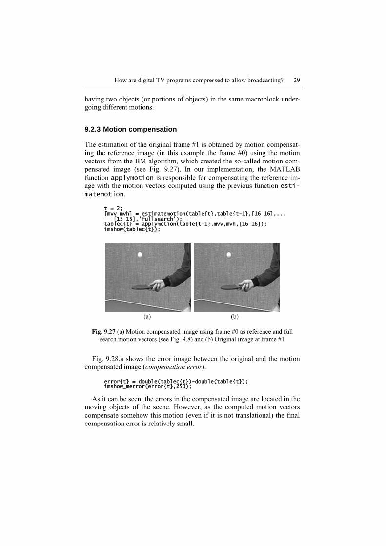
9.2.3 Motion compensation
The estimation of the original frame #1 is obtained by motion compensat-
ing the reference image (in this example the frame #0) using the motion
vectors from the BM algorithm, which created the so-called motion com-
pensated image (see Fig. 9.27). In our implementation, the MATLAB
function applymotion is responsible for compensating the reference im-
age with the motion vectors computed using the previous function esti-
matemotion.
t = 2; [mvv mvh] = estimatemotion(table{t},table{t-1},[16 16],... [15 15],'fullsearch'); tablec{t} = applymotion(table{t-1},mvv,mvh,[16 16]); imshow(tablec{t});
(a) (b)
Fig. 9.27 (a) Motion compensated image using frame #0 as reference and full
search motion vectors (see Fig. 9.8) and (b) Original image at frame #1
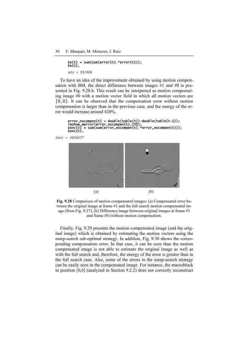
Fig. 9.28.a shows the error image between the original and the motion
compensated image (compensation error).
error{t} = double(tablec{t})-double(table{t}); imshow_merror(error{t},250);
As it can be seen, the errors in the compensated image are located in the
moving objects of the scene. However, as the computed motion vectors
compensate somehow this motion (even if it is not translational) the final
compensation error is relatively small.
30 F. Marqués, M. Menezes, J. Ruiz
Ee{t} = sum(sum(error{t}.*error{t})); Ee{t}, ans = 932406
To have an idea of the improvement obtained by using motion compen-
sation with BM, the direct difference between images #1 and #0 is pre-
sented in Fig. 9.28.b. This result can be interpreted as motion compensat-
ing image #0 with a motion vector field in which all motion vectors are
[0,0]. It can be observed that the compensation error without motion
compensation is larger than in the previous case, and the energy of the er-
ror would increase around 420%.
error_nocompen{t} = double(table{t})-double(table{t-1}); imshow_merror(error_nocompen{t},250); Eenc{t} = sum(sum(error_nocompen{t}.*error_nocompen{t})); Eenc{t},
Eenc = 4836677
(a) (b)
Fig. 9.28 Comparison of motion compensated images: (a) Compensated error be-
tween the original image at frame #1 and the full search motion compensated im-
age (from Fig. 9.27), (b) Difference image between original images at frame #1
and frame #0 (without motion compensation.
Finally, Fig. 9.29 presents the motion compensated image (and the orig-
inal image) which is obtained by estimating the motion vectors using the
nstep-search sub-optimal strategy. In addition, Fig. 9.30 shows the corres-
ponding compensation error. In that case, it can be seen than the motion
compensated image is not able to estimate the original image as well as
with the full search and, therefore, the energy of the error is greater than in
the full search case. Also, some of the errors in the nstep-search strategy
can be easily seen in the compensated image. For instance, the macroblock
in position [6,6] (analyzed in Section 9.2.2) does not correctly reconstruct
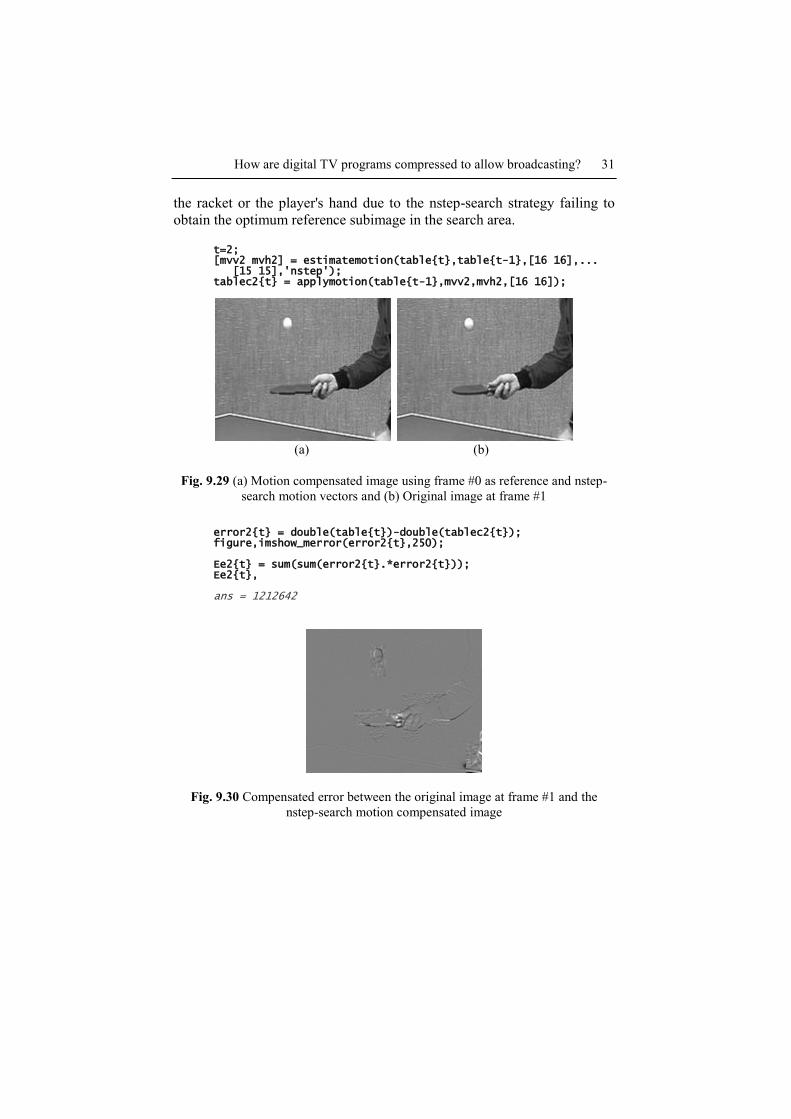
How are digital TV programs compressed to allow broadcasting? 31
the racket or the player's hand due to the nstep-search strategy failing to
obtain the optimum reference subimage in the search area.
t=2; [mvv2 mvh2] = estimatemotion(table{t},table{t-1},[16 16],... [15 15],'nstep'); tablec2{t} = applymotion(table{t-1},mvv2,mvh2,[16 16]);
(a) (b)
Fig. 9.29 (a) Motion compensated image using frame #0 as reference and nstep-
search motion vectors and (b) Original image at frame #1
error2{t} = double(table{t})-double(tablec2{t}); figure,imshow_merror(error2{t},250); Ee2{t} = sum(sum(error2{t}.*error2{t})); Ee2{t}, ans = 1212642
Fig. 9.30 Compensated error between the original image at frame #1 and the
nstep-search motion compensated image
32 F. Marqués, M. Menezes, J. Ruiz
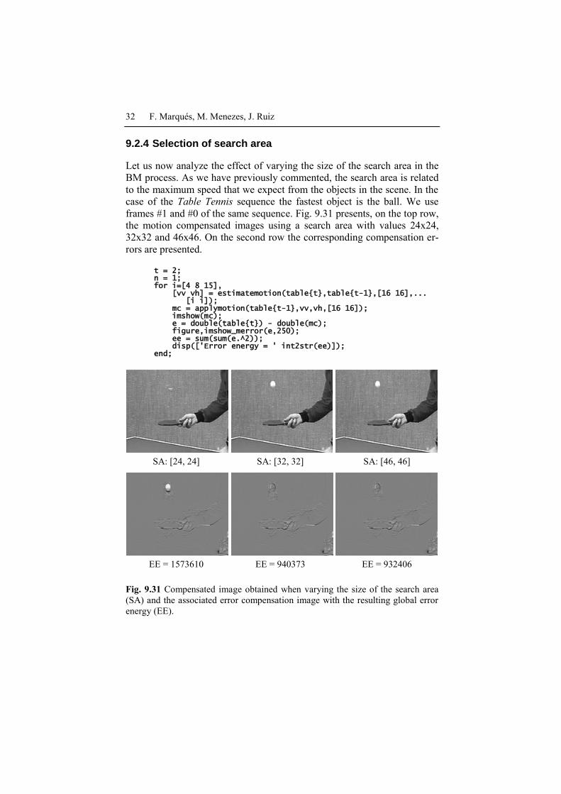
9.2.4 Selection of search area
Let us now analyze the effect of varying the size of the search area in the
BM process. As we have previously commented, the search area is related
to the maximum speed that we expect from the objects in the scene. In the
case of the Table Tennis sequence the fastest object is the ball. We use
frames #1 and #0 of the same sequence. Fig. 9.31 presents, on the top row,
the motion compensated images using a search area with values 24x24,
32x32 and 46x46. On the second row the corresponding compensation er-
rors are presented.
t = 2; n = 1; for i=[4 8 15], [vv vh] = estimatemotion(table{t},table{t-1},[16 16],... [i i]); mc = applymotion(table{t-1},vv,vh,[16 16]); imshow(mc); e = double(table{t}) - double(mc); figure,imshow_merror(e,250); ee = sum(sum(e.^2)); disp(['Error energy = ' int2str(ee)]); end;
SA: [24, 24] SA: [32, 32] SA: [46, 46]
EE = 1573610 EE = 940373 EE = 932406
Fig. 9.31 Compensated image obtained when varying the size of the search area
(SA) and the associated error compensation image with the resulting global error
energy (EE).
How are digital TV programs compressed to allow broadcasting? 33
As it can be seen, a search area as small as 24x24 (corresponding to a
maximum motion vector displacement of [±4, ±4]) does not allow correct-
ly compensating the ball since its motion has displaced it outside the
search area. This can be easily seen on the first column of Fig. 9.31 where
the ball does not appear in the motion compensated image (so the error in
the area of the ball is very high). However, when using a search area of
32x32 or 46x46, the BM is capable of following the ball movement and
the corresponding motion compensated images provide smaller errors in
the area of the ball.
Of course, the use of larger search areas implies a trade-off: the quality
of the motion vectors is increased at the expenses of analyzing a larger
amount of possible displacements and, therefore, increasing the computa-
tional load of the motion estimation step.
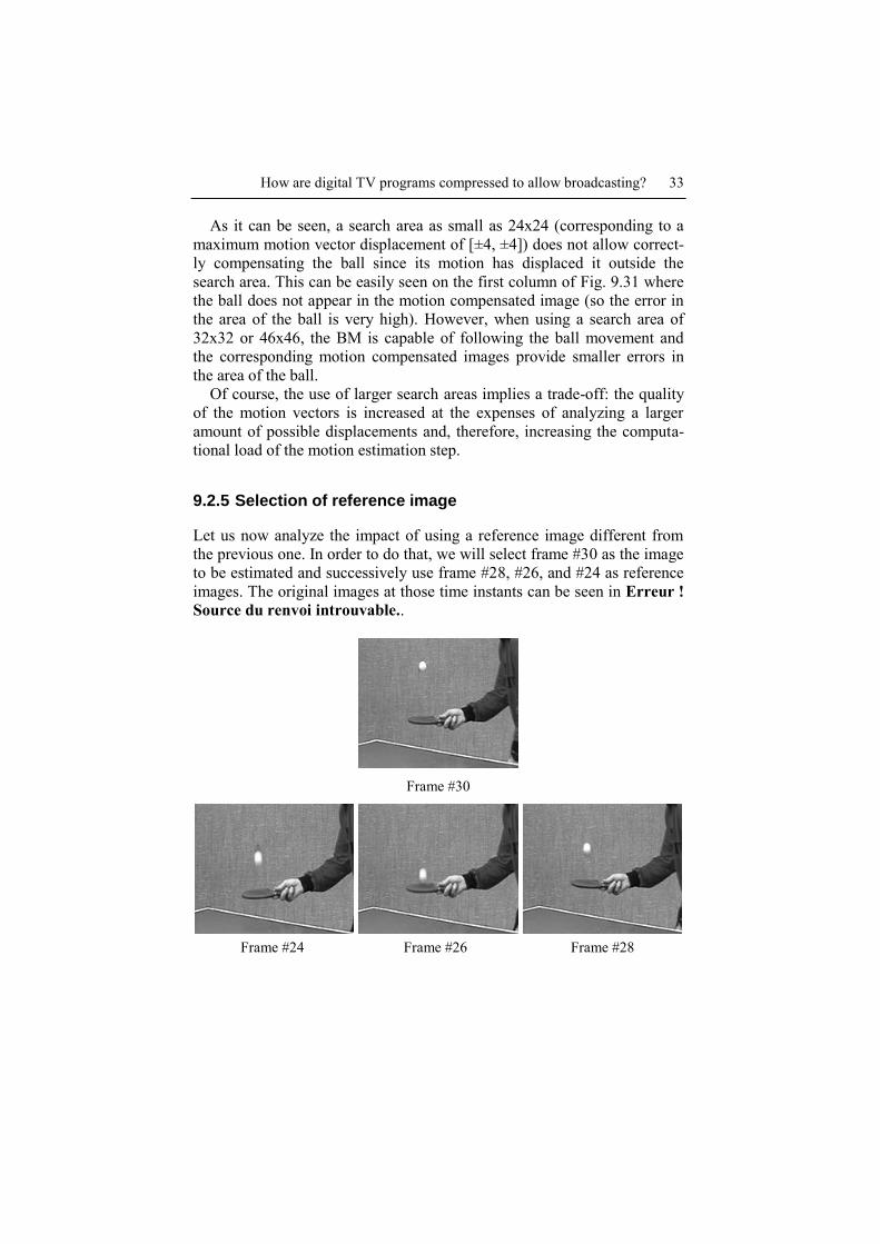
9.2.5 Selection of reference image
Let us now analyze the impact of using a reference image different from
the previous one. In order to do that, we will select frame #30 as the image
to be estimated and successively use frame #28, #26, and #24 as reference
images. The original images at those time instants can be seen in Erreur !
Source du renvoi introuvable..
Frame #30
Frame #24 Frame #26 Frame #28
34 F. Marqués, M. Menezes, J. Ruiz
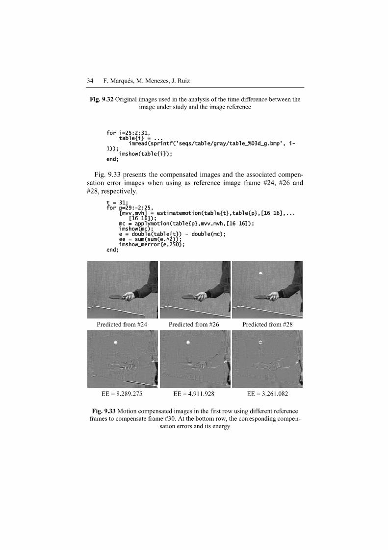
Fig. 9.32 Original images used in the analysis of the time difference between the
image under study and the image reference
for i=25:2:31, table{i} = ... imread(sprintf('seqs/table/gray/table_%03d_g.bmp', i-1)); imshow(table{i}); end;
Fig. 9.33 presents the compensated images and the associated compen-
sation error images when using as reference image frame #24, #26 and
#28, respectively. t = 31; for p=29:-2:25, [mvv,mvh] = estimatemotion(table{t},table{p},[16 16],... [16 16]); mc = applymotion(table{p},mvv,mvh,[16 16]); imshow(mc); e = double(table{t}) - double(mc); ee = sum(sum(e.^2)); imshow_merror(e,250); end;
Predicted from #24 Predicted from #26 Predicted from #28
EE = 8.289.275 EE = 4.911.928 EE = 3.261.082
Fig. 9.33 Motion compensated images in the first row using different reference
frames to compensate frame #30. At the bottom row, the corresponding compen-
sation errors and its energy
How are digital TV programs compressed to allow broadcasting? 35
As it can be seen, the further away the two images, the higher the energy
of the compensation error. This is due to the fact that distant images are
less correlated and, therefore, the prediction step cannot exploit in an effi-
cient manner the temporal correlation. Moreover, there is an object, the
player's arm at the bottom right corner, in frame #30 which is not present
in frames #24 and #26. Therefore, when using these frames as references,
this object does not have any referent in the reference image and the mo-
tion compensation leads to a compensation error with higher energy.
9.2.6 Backward motion estimation
The problem of having an object in the current frame without any referent
in the previous images happens every time an object appears in the scene.
It is clear that, in order to obtain a referent for this object, we should look
into the future frames; that is, use a non-causal prediction. At this stage,
we are only going to analyze the possibility of using past as well as future
frames as reference images. We postpone to Section 9.2.9 the illustration
of how this non-causal prediction can actually be implemented in the cod-
ing context (see Section 9.1.2).
Here, we analyze the possibility of estimating the current frame using as
reference image the following frame in the sequence. If non-causal predic-
tion can be used (that is, motion compensate future frames is possible), the
information in past and future images can be used separately or combined
in order to obtain a better motion compensated image. These concepts are
illustrated in the next Figures.
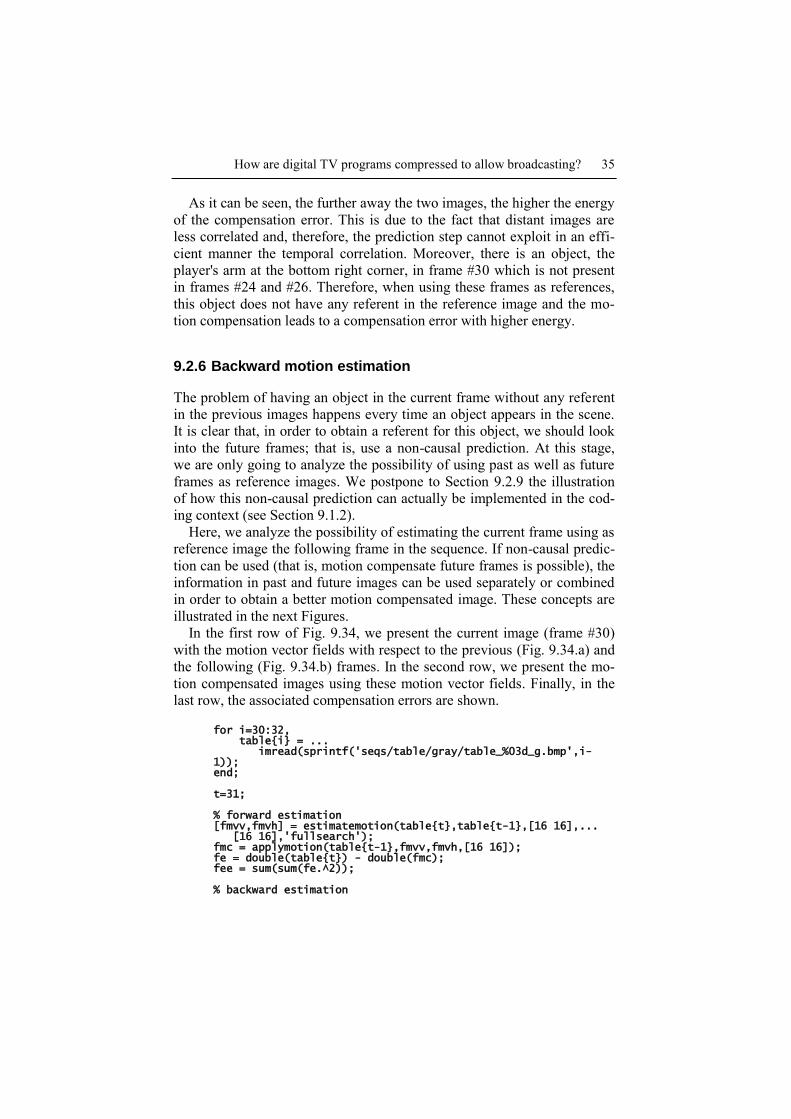
In the first row of Fig. 9.34, we present the current image (frame #30)
with the motion vector fields with respect to the previous (Fig. 9.34.a) and
the following (Fig. 9.34.b) frames. In the second row, we present the mo-
tion compensated images using these motion vector fields. Finally, in the
last row, the associated compensation errors are shown.
for i=30:32, table{i} = ... imread(sprintf('seqs/table/gray/table_%03d_g.bmp',i-1)); end; t=31; % forward estimation [fmvv,fmvh] = estimatemotion(table{t},table{t-1},[16 16],... [16 16],'fullsearch'); fmc = applymotion(table{t-1},fmvv,fmvh,[16 16]); fe = double(table{t}) - double(fmc); fee = sum(sum(fe.^2)); % backward estimation
36 F. Marqués, M. Menezes, J. Ruiz
[bmvv,bmvh] = estimatemotion(table{t},table{t+1},[16 16], ... [16 16],'fullsearch'); bmc = applymotion(table{t+1},bmvv,bmvh,[16 16]); be = double(table{t}) - double(bmc); bee = sum(sum(be.^2));
MV with reference #29 MVs with reference #31
Forward motion compensated image Backward motion compensated image
Error energy = 2.081.546 Error energy = 1.091.744
Fig. 9.34 Motion estimation and compensation using forward (#29) and backward
(#31) references for frame #30
From the example above it is clear than backward motion estimation can
reduce the compensation error especially when new objects appear in the
scene. In this example, this is the case of the player‟s arm as well as a part
of the background (note that the camera is zooming-out). However, in or-
der to further reduce the compensation error, both motion compensated
How are digital TV programs compressed to allow broadcasting? 37
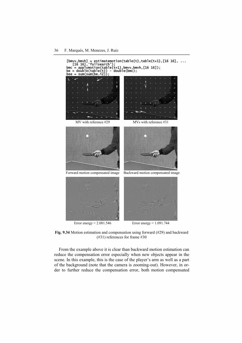
images (forward and backward) could be combined. Following this new
idea, Fig. 9.35 shows the motion compensated image and the compensa-
tion error where, for each macroblock, the estimation is computed by li-
nearly combining the two reference subimages with equal weights (w =
0.5). bdmc = uint8(0.5 * (double(fmc) + double(bmc))); bde = double(table{t}) - double(bdmc); bdee = sum(sum(bde.^2)); imshow(bdmc);imshow_merror(bde,250);
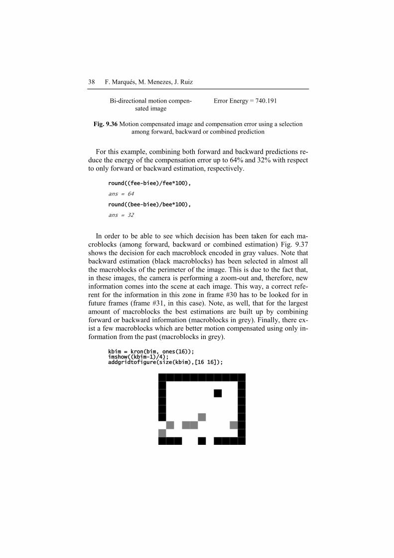
Bi-directional motion compen-
sated image
Error Energy = 936.236
Fig. 9.35 Motion compensated image and compensation error using combined
forward and backward prediction
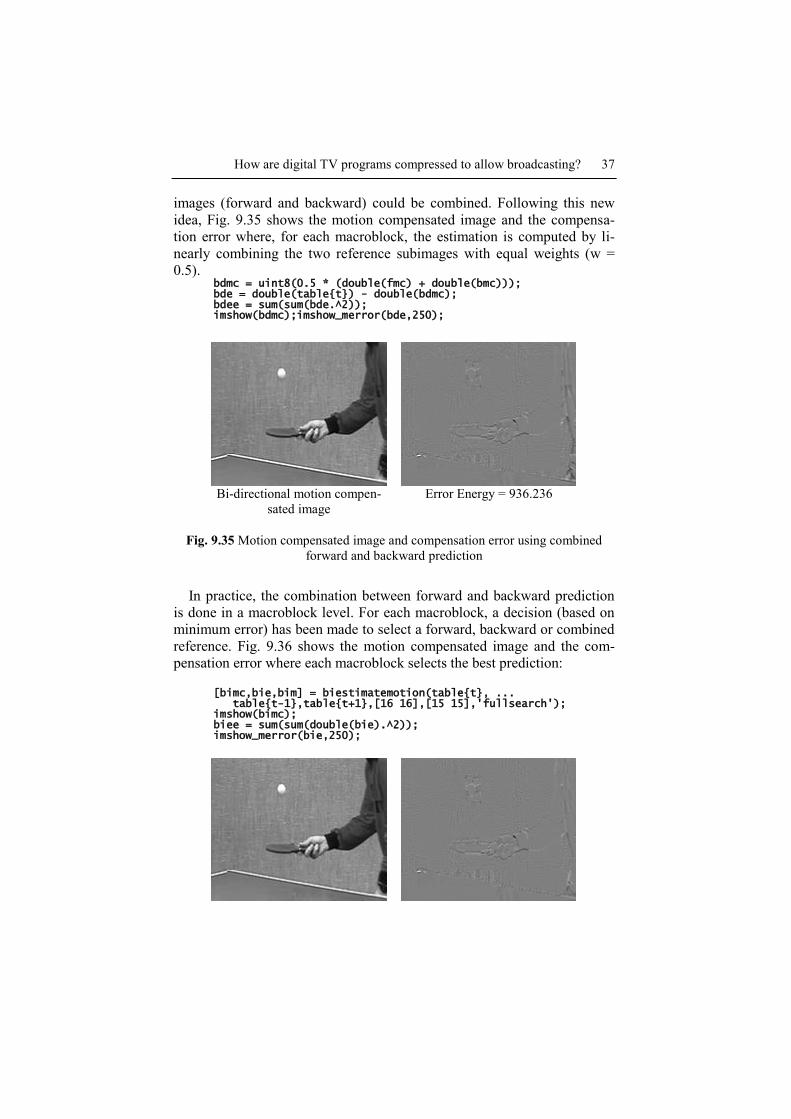
In practice, the combination between forward and backward prediction
is done in a macroblock level. For each macroblock, a decision (based on
minimum error) has been made to select a forward, backward or combined
reference. Fig. 9.36 shows the motion compensated image and the com-
pensation error where each macroblock selects the best prediction:
[bimc,bie,bim] = biestimatemotion(table{t}, ... table{t-1},table{t+1},[16 16],[15 15],'fullsearch'); imshow(bimc); biee = sum(sum(double(bie).^2)); imshow_merror(bie,250);
38 F. Marqués, M. Menezes, J. Ruiz
Bi-directional motion compen-
sated image
Error Energy = 740.191
Fig. 9.36 Motion compensated image and compensation error using a selection
among forward, backward or combined prediction
For this example, combining both forward and backward predictions re-
duce the energy of the compensation error up to 64% and 32% with respect
to only forward or backward estimation, respectively.
round((fee-biee)/fee*100), ans = 64 round((bee-biee)/bee*100), ans = 32
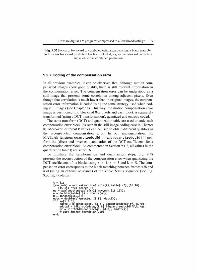
In order to be able to see which decision has been taken for each ma-
croblocks (among forward, backward or combined estimation) Fig. 9.37
shows the decision for each macroblock encoded in gray values. Note that
backward estimation (black macroblocks) has been selected in almost all
the macroblocks of the perimeter of the image. This is due to the fact that,
in these images, the camera is performing a zoom-out and, therefore, new
information comes into the scene at each image. This way, a correct refe-
rent for the information in this zone in frame #30 has to be looked for in
future frames (frame #31, in this case). Note, as well, that for the largest
amount of macroblocks the best estimations are built up by combining
forward or backward information (macroblocks in grey). Finally, there ex-
ist a few macroblocks which are better motion compensated using only in-
formation from the past (macroblocks in grey).
kbim = kron(bim, ones(16)); imshow((kbim-1)/4); addgridtofigure(size(kbim),[16 16]);
How are digital TV programs compressed to allow broadcasting? 39
Fig. 9.37 Forward, backward or combined estimation decision: a black macrob-
lock means backward prediction has been selected, a gray one forward prediction
and a white one combined prediction
9.2.7 Coding of the compensation error
In all previous examples, it can be observed that, although motion com-
pensated images show good quality, there is still relevant information in
the compensation error. The compensation error can be understood as a
still image that presents some correlation among adjacent pixels. Even
though that correlation is much lower than in original images, the compen-
sation error information is coded using the same strategy used when cod-
ing still images (see Chapter 8). This way, the motion compensation error
image is partitioned into blocks of 8x8 pixels and each block is separately
transformed (using a DCT transformation), quantized and entropy coded.
The same transform (DCT) and quantization table are used to code each
compensation error block (as seen in the still image coding case in Chapter
8). Moreover, different k values can be used to obtain different qualities in
the reconstructed compensation error. In our implementation, the
MATLAB functions quantizedct8diff and iquantizedct8diff per-
form the (direct and inverse) quantization of the DCT coefficients for a
compensation error block. As commented in Section 9.1.2, all values in the
quantization table Q are set to 16.
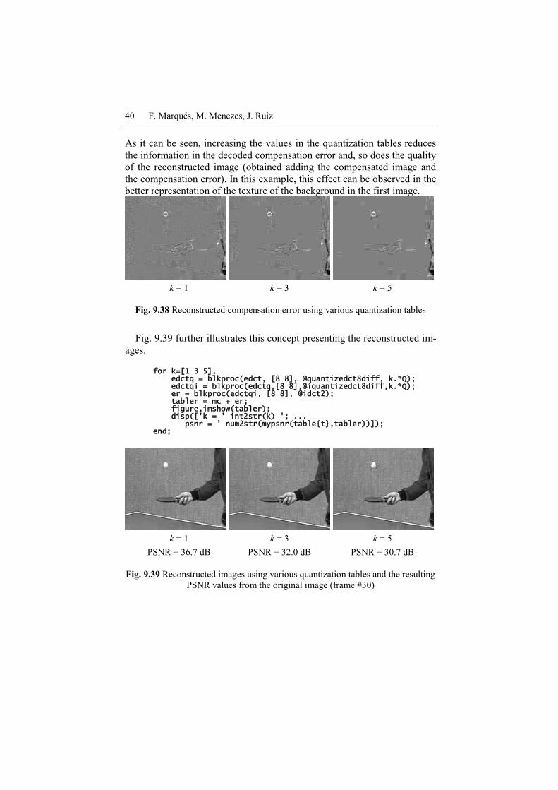
To illustrate the transformation and quantization steps, Fig. 9.38
presents the reconstruction of the compensation error when quantizing the
DCT coefficients of its blocks using k = 1, k = 3 and k = 5. The com-
pensation error corresponds to the block matching between frames #28 and
#30 (using an exhaustive search) of the Table Tennis sequence (see Fig.
9.33 right column).
t = 31; [mvv,mvh] = estimatemotion(table{t},table{t-2},[16 16],... [15 15],'fullsearch'); mc = applymotion(table{t-2},mvv,mvh,[16 16]); e = double(table{t}) - double(mc); Q = 16*ones(16,16); edct = double(blkproc(e, [8 8], @dct2)); for k=[1 3 5], edctq = blkproc(edct, [8 8], @quantizedct8diff, k.*Q); edctqi = blkproc(edctq,[8 8],@iquantizedct8diff,k.*Q); er = uint8(blkproc(edctqi, [8 8], @idct2)); figure,imshow_merror(er,250); end;
40 F. Marqués, M. Menezes, J. Ruiz
As it can be seen, increasing the values in the quantization tables reduces
the information in the decoded compensation error and, so does the quality
of the reconstructed image (obtained adding the compensated image and
the compensation error). In this example, this effect can be observed in the
better representation of the texture of the background in the first image.
k = 1 k = 3 k = 5
Fig. 9.38 Reconstructed compensation error using various quantization tables
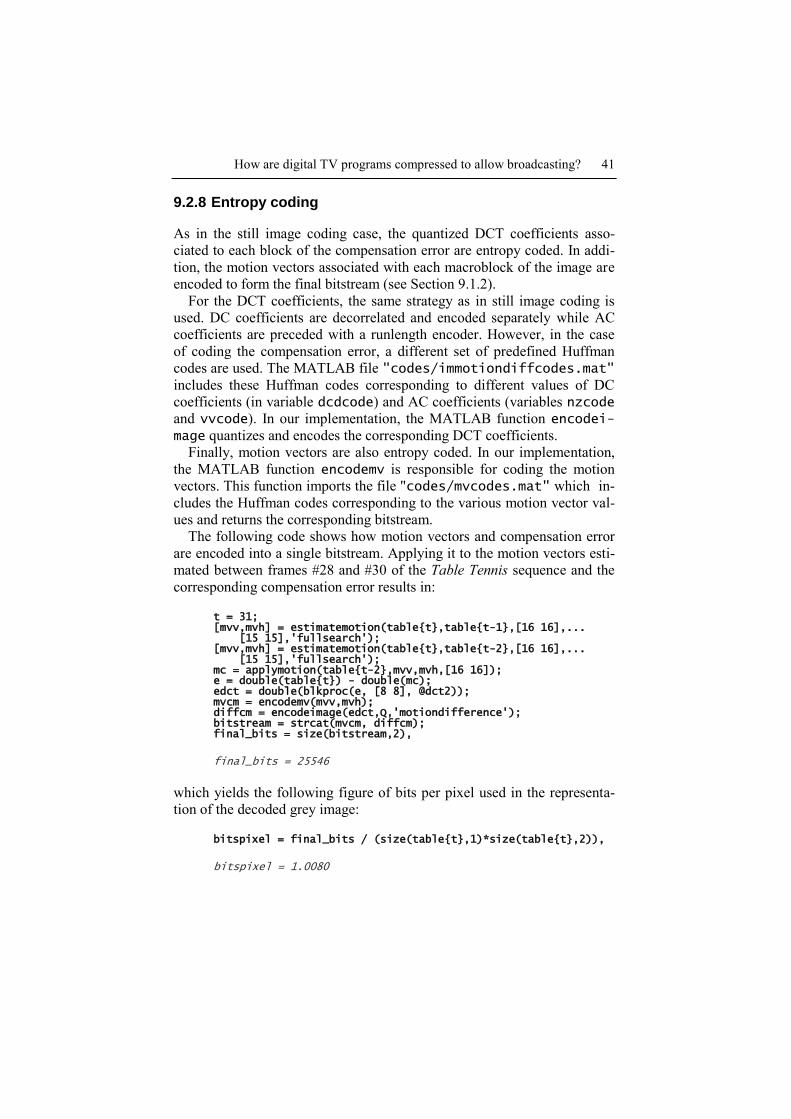
Fig. 9.39 further illustrates this concept presenting the reconstructed im-
ages.
for k=[1 3 5], edctq = blkproc(edct, [8 8], @quantizedct8diff, k.*Q); edctqi = blkproc(edctq,[8 8],@iquantizedct8diff,k.*Q); er = blkproc(edctqi, [8 8], @idct2); tabler = mc + er; figure,imshow(tabler); disp(['k = ' int2str(k) '; ... psnr = ' num2str(mypsnr(table{t},tabler))]); end;
k = 1
PSNR = 36.7 dB
k = 3
PSNR = 32.0 dB
k = 5
PSNR = 30.7 dB
Fig. 9.39 Reconstructed images using various quantization tables and the resulting
PSNR values from the original image (frame #30)
How are digital TV programs compressed to allow broadcasting? 41
9.2.8 Entropy coding
As in the still image coding case, the quantized DCT coefficients asso-
ciated to each block of the compensation error are entropy coded. In addi-
tion, the motion vectors associated with each macroblock of the image are
encoded to form the final bitstream (see Section 9.1.2).
For the DCT coefficients, the same strategy as in still image coding is
used. DC coefficients are decorrelated and encoded separately while AC
coefficients are preceded with a runlength encoder. However, in the case
of coding the compensation error, a different set of predefined Huffman
codes are used. The MATLAB file "codes/immotiondiffcodes.mat"
includes these Huffman codes corresponding to different values of DC
coefficients (in variable dcdcode) and AC coefficients (variables nzcode
and vvcode). In our implementation, the MATLAB function encodei-
mage quantizes and encodes the corresponding DCT coefficients.
Finally, motion vectors are also entropy coded. In our implementation,
the MATLAB function encodemv is responsible for coding the motion
vectors. This function imports the file "codes/mvcodes.mat" which in-
cludes the Huffman codes corresponding to the various motion vector val-
ues and returns the corresponding bitstream.
The following code shows how motion vectors and compensation error
are encoded into a single bitstream. Applying it to the motion vectors esti-
mated between frames #28 and #30 of the Table Tennis sequence and the
corresponding compensation error results in:
t = 31; [mvv,mvh] = estimatemotion(table{t},table{t-1},[16 16],... [15 15],'fullsearch'); [mvv,mvh] = estimatemotion(table{t},table{t-2},[16 16],... [15 15],'fullsearch'); mc = applymotion(table{t-2},mvv,mvh,[16 16]); e = double(table{t}) - double(mc); edct = double(blkproc(e, [8 8], @dct2)); mvcm = encodemv(mvv,mvh); diffcm = encodeimage(edct,Q,'motiondifference'); bitstream = strcat(mvcm, diffcm); final_bits = size(bitstream,2),
final_bits = 25546
which yields the following figure of bits per pixel used in the representa-
tion of the decoded grey image:
bitspixel = final_bits / (size(table{t},1)*size(table{t},2)),
bitspixel = 1.0080
42 F. Marqués, M. Menezes, J. Ruiz
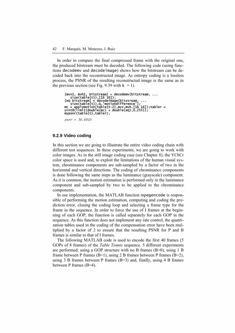
In order to compare the final compressed frame with the original one,
the produced bitstream must be decoded. The following code (using func-
tions decodemv and decodeimage) shows how the bitstream can be de-
coded back into the reconstructed image. As entropy coding is a lossless
process, the PSNR of the resulting reconstructed image is the same as in
the previous section (see Fig. 9.39 with k = 1).
[mvv2, mvh2, bitstream] = decodemv(bitstream, ... size(table{t}),[16 16]); [eQ bitstream] = decodeimage(bitstream, ... size(table{t}),Q,'motiondifference'); mc = applymotion(table{t-2},mvv,mvh,[16 16]);tabler = uint8(limit(double(mc) + double(eQ),0,255)); mypsnr(table{t},tabler),
psnr = 36.6910
9.2.9 Video coding
In this section we are going to illustrate the entire video coding chain with
different test sequences. In these experiments, we are going to work with
color images. As in the still image coding case (see Chapter 8), the YCbCr
color space is used and, to exploit the limitations of the human visual sys-
tem, chrominance components are sub-sampled by a factor of two in the
horizontal and vertical directions. The coding of chrominance components
is done following the same steps as the luminance (grayscale) component.
As it is common, the motion estimation is performed only in the luminance
component and sub-sampled by two to be applied to the chrominance
components.
In our implementation, the MATLAB function mpegencode is respon-
sible of performing the motion estimation, computing and coding the pre-
diction error, closing the coding loop and selecting a frame type for the
frame in the sequence. In order to force the use of I frames at the begin-
ning of each GOP, the function is called separately for each GOP in the
sequence. As this function does not implement any rate control, the quanti-
zation tables used in the coding of the compensation error have been mul-
tiplied by a factor of 2 to ensure that the resulting PSNR for P and B
frames is similar to that of I frames.
The following MATLAB code is used to encode the first 40 frames (5
GOPs of 8 frames) of the Table Tennis sequence. 5 different experiments
are performed; using a GOP structure with no B frames (B=0), using 1 B
frame between P frames (B=1), using 2 B frames between P frames (B=2),
using 3 B frames between P frames (B=3) and, finally, using 4 B frames
between P frames (B=4).
How are digital TV programs compressed to allow broadcasting? 43
ngops = 5; gopsize = 8; for ng = 1:ngops, [cm,bits{1},type{1},psnr{1}] = mpegencode( ... 'results/table_color','seqs/table/color', ... 1+(ng-1)*gopsize,ng*gopsize, 1,gopsize); [cm,bits{2},type{2},psnr{2}] = mpegencode(... 'results/table_color','seqs/table/color', ... 1+(ng-1)*gopsize,ng*gopsize+1,2,round(gopsize/2)); [cm,bits{3},type{3},psnr{3}] = mpegencode(... 'results/table_color','seqs/table/color', ... 1+(ng-1)*gopsize,ng*gopsize+1,3,3); [cm,bits{4},type{4},psnr{4}] = mpegencode(... 'results/table_color','seqs/table/color', ... 1+(ng-1)*gopsize,ng*gopsize+1,4,2); [cm,bits{5},type{5},psnr{5}] = mpegencode(... 'results/table_color','seqs/table/color', ... 1+(ng-1)*gopsize,ng*gopsize+1,5,2);
for i=1:5, table.bits{i}(1+(ng-1)*gopsize:ng*gopsize) = ... bits{i}(1+(ng-1)*gopsize:ng*gopsize); table.type{i}(1+(ng-1)*gopsize:ng*gopsize) = ... type{i}(1+(ng-1)*gopsize:ng*gopsize); table.psnr{i}.y(1+(ng-1)*gopsize:ng*gopsize) = ... psnr{i}.y(1+(ng-1)*gopsize:ng*gopsize); table.psnr{i}.cb(1+(ng-1)*gopsize:ng*gopsize) = ... psnr{i}.cb(1+(ng-1)*gopsize:ng*gopsize); table.psnr{i}.cr(1+(ng-1)*gopsize:ng*gopsize) = ... psnr{i}.cr(1+(ng-1)*gopsize:ng*gopsize); end; end;
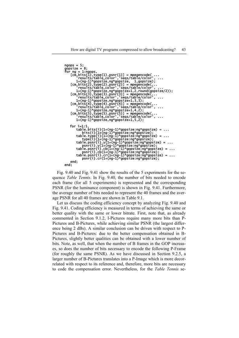
Fig. 9.40 and Fig. 9.41 show the results of the 5 experiments for the se-
quence Table Tennis. In Fig. 9.40, the number of bits needed to encode
each frame (for all 5 experiments) is represented and the corresponding
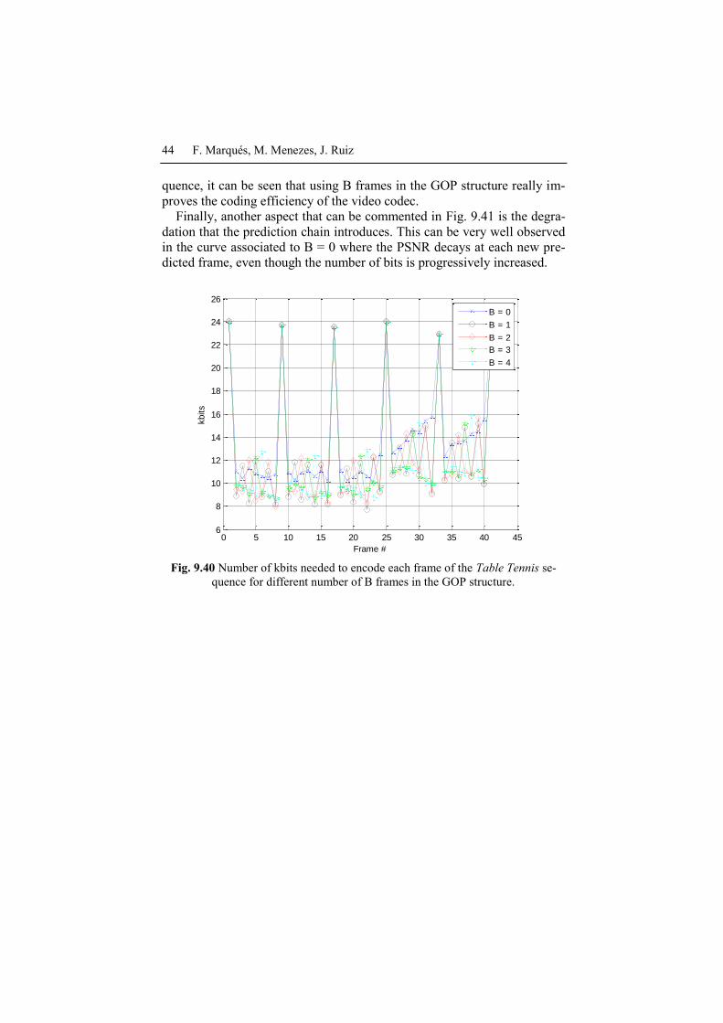
PSNR (for the luminance component) is shown in Fig. 9.41. Furthermore,
the average number of bits needed to represent the 40 frames and the aver-
age PSNR for all 40 frames are shown in Table 9.1.
Let us discuss the coding efficiency concept by analyzing Fig. 9.40 and
Fig. 9.41. Coding efficiency is measured in terms of achieving the same or
better quality with the same or lower bitrate. First, note that, as already
commented in Section 9.1.2, I-Pictures require many more bits than P-
Pictures and B-Pictures, while achieving similar PSNR (the largest differ-
ence being 2 dBs). A similar conclusion can be driven with respect to P-
Pictures and B-Pictures: due to the better compensation obtained in B-
Pictures, slightly better qualities can be obtained with a lower number of
bits. Note, as well, that when the number of B frames in the GOP increas-
es, so does the number of bits necessary to encode the following P-Frame
(for roughly the same PSNR). As we have discussed in Section 9.2.5, a
larger number of B-Pictures translates into a P-Image which is more decor-
related with respect to its reference and, therefore, more bits are necessary
to code the compensation error. Nevertheless, for the Table Tennis se-
44 F. Marqués, M. Menezes, J. Ruiz
quence, it can be seen that using B frames in the GOP structure really im-
proves the coding efficiency of the video codec.
Finally, another aspect that can be commented in Fig. 9.41 is the degra-
dation that the prediction chain introduces. This can be very well observed
in the curve associated to B = 0 where the PSNR decays at each new pre-
dicted frame, even though the number of bits is progressively increased.
0 5 10 15 20 25 30 35 40 456
8
10
12
14
16
18
20
22
24
26
Frame #
kbits
B = 0
B = 1
B = 2
B = 3
B = 4
Fig. 9.40 Number of kbits needed to encode each frame of the Table Tennis se-
quence for different number of B frames in the GOP structure.
How are digital TV programs compressed to allow broadcasting? 45
0 5 10 15 20 25 30 35 40 4531.5
32
32.5
33
33.5
34
34.5
35
Frame #
PS
NR
Y [
dB
]
B = 0
B = 1
B = 2
B = 3
B = 4
Fig. 9.41 Resulting PSNR (luminance component) for each frame of the Table
Tennis sequence for different number of B frames in the GOP structure.
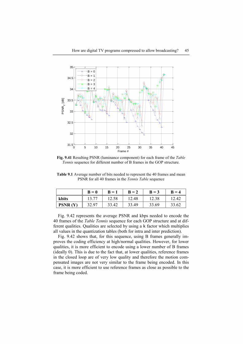
Table 9.1 Average number of bits needed to represent the 40 frames and mean
PSNR for all 40 frames in the Tennis Table sequence
B = 0 B = 1 B = 2 B = 3 B = 4
kbits 13.77 12.58 12.48 12.38 12.42
PSNR (Y) 32.97 33.42 33.49 33.69 33.62
Fig. 9.42 represents the average PSNR and kbps needed to encode the
40 frames of the Table Tennis sequence for each GOP structure and at dif-
ferent qualities. Qualities are selected by using a k factor which multiplies
all values in the quantization tables (both for intra and inter prediction).
Fig. 9.42 shows that, for this sequence, using B frames generally im-
proves the coding efficiency at high/normal qualities. However, for lower
qualities, it is more efficient to encode using a lower number of B frames
(ideally 0). This is due to the fact that, at lower qualities, reference frames
in the closed loop are of very low quality and therefore the motion com-
pensated images are not very similar to the frame being encoded. In this
case, it is more efficient to use reference frames as close as possible to the
frame being coded.
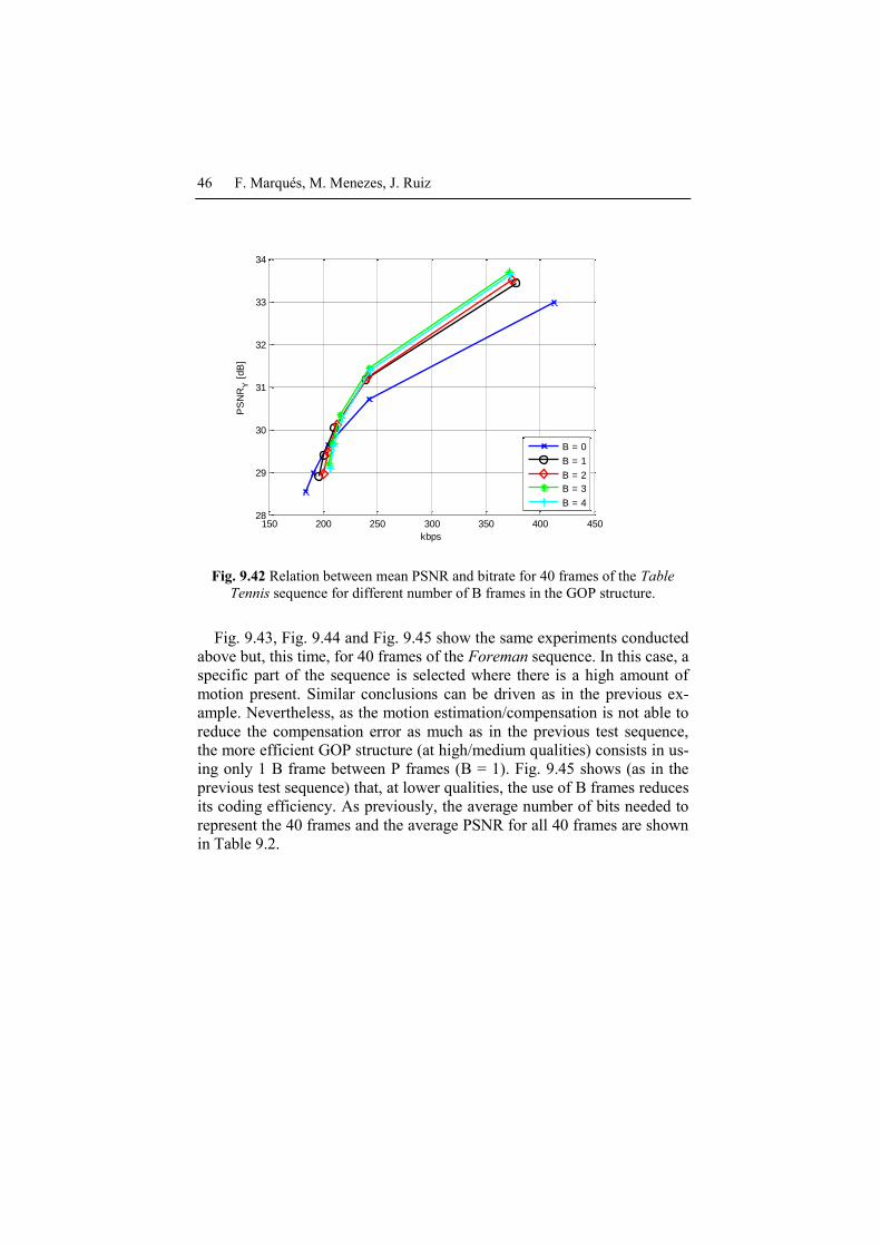
46 F. Marqués, M. Menezes, J. Ruiz
150 200 250 300 350 400 45028
29
30
31
32
33
34
kbps
PS
NR
Y [
dB
]
B = 0
B = 1
B = 2
B = 3
B = 4
Fig. 9.42 Relation between mean PSNR and bitrate for 40 frames of the Table
Tennis sequence for different number of B frames in the GOP structure.
Fig. 9.43, Fig. 9.44 and Fig. 9.45 show the same experiments conducted
above but, this time, for 40 frames of the Foreman sequence. In this case, a
specific part of the sequence is selected where there is a high amount of
motion present. Similar conclusions can be driven as in the previous ex-
ample. Nevertheless, as the motion estimation/compensation is not able to
reduce the compensation error as much as in the previous test sequence,
the more efficient GOP structure (at high/medium qualities) consists in us-
ing only 1 B frame between P frames (B = 1). Fig. 9.45 shows (as in the
previous test sequence) that, at lower qualities, the use of B frames reduces
its coding efficiency. As previously, the average number of bits needed to
represent the 40 frames and the average PSNR for all 40 frames are shown
in Table 9.2.
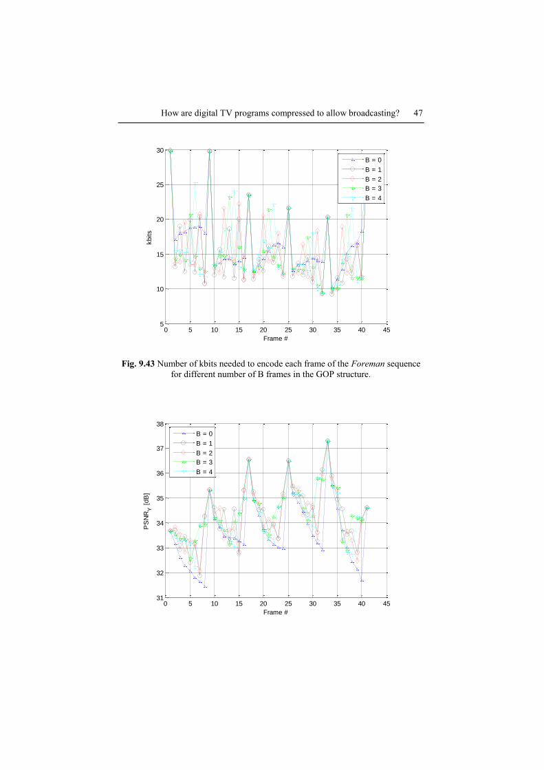
How are digital TV programs compressed to allow broadcasting? 47
0 5 10 15 20 25 30 35 40 455
10
15
20
25
30
Frame #
kbits
B = 0
B = 1
B = 2
B = 3
B = 4
Fig. 9.43 Number of kbits needed to encode each frame of the Foreman sequence
for different number of B frames in the GOP structure.
0 5 10 15 20 25 30 35 40 4531
32
33
34
35
36
37
38
Frame #
PS
NR
Y [
dB
]
B = 0
B = 1
B = 2
B = 3
B = 4
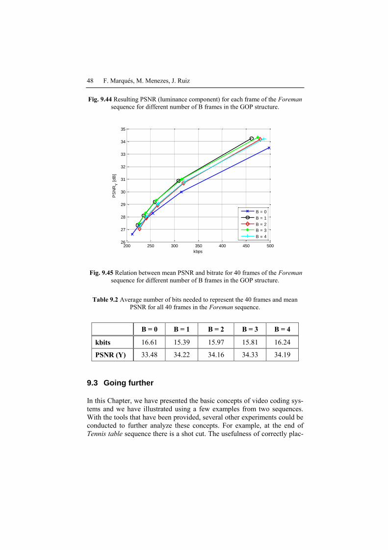
48 F. Marqués, M. Menezes, J. Ruiz
Fig. 9.44 Resulting PSNR (luminance component) for each frame of the Foreman
sequence for different number of B frames in the GOP structure.
200 250 300 350 400 450 50026
27
28
29
30
31
32
33
34
35
kbps
PS
NR
Y [
dB
]
B = 0
B = 1
B = 2
B = 3
B = 4
Fig. 9.45 Relation between mean PSNR and bitrate for 40 frames of the Foreman
sequence for different number of B frames in the GOP structure.
Table 9.2 Average number of bits needed to represent the 40 frames and mean
PSNR for all 40 frames in the Foreman sequence.
B = 0 B = 1 B = 2 B = 3 B = 4
kbits 16.61 15.39 15.97 15.81 16.24
PSNR (Y) 33.48 34.22 34.16 34.33 34.19
9.3 Going further
In this Chapter, we have presented the basic concepts of video coding sys-
tems and we have illustrated using a few examples from two sequences.
With the tools that have been provided, several other experiments could be
conducted to further analyze these concepts. For example, at the end of
Tennis table sequence there is a shot cut. The usefulness of correctly plac-
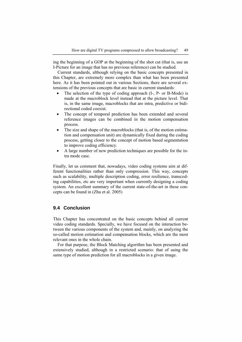
How are digital TV programs compressed to allow broadcasting? 49
ing the beginning of a GOP at the beginning of the shot cut (that is, use an
I-Picture for an image that has no previous reference) can be studied.
Current standards, although relying on the basic concepts presented in
this Chapter, are extremely more complex than what has been presented
here. As it has been pointed out in various Sections, there are several ex-
tensions of the previous concepts that are basic in current standards:
The selection of the type of coding approach (I-, P- or B-Mode) is
made at the macroblock level instead that at the picture level. That
is, in the same image, macroblocks that are intra, predictive or bidi-
rectional coded coexist.
The concept of temporal prediction has been extended and several
reference images can be combined in the motion compensation
process.
The size and shape of the macroblocks (that is, of the motion estima-
tion and compensation unit) are dynamically fixed during the coding
process, getting closer to the concept of motion based segmentation
to improve coding efficiency.
A large number of new prediction techniques are possible for the in-
tra mode case.
Finally, let us comment that, nowadays, video coding systems aim at dif-
ferent functionalities rather than only compression. This way, concepts
such as scalability, multiple description coding, error resilience, transcod-
ing capabilities, etc are very important when currently designing a coding
system. An excellent summary of the current state-of-the-art in these con-
cepts can be found in (Zhu et al. 2005)
9.4 Conclusion
This Chapter has concentrated on the basic concepts behind all current
video coding standards. Specially, we have focused on the interaction be-
tween the various components of the system and, mainly, on analyzing the
so-called motion estimation and compensation blocks, which are the most
relevant ones in the whole chain.
For that purpose, the Block Matching algorithm has been presented and
extensively studied, although in a restricted scenario: that of using the
same type of motion prediction for all macroblocks in a given image.
50 F. Marqués, M. Menezes, J. Ruiz
9.5 References
Rec. ITU-R BT.601 (1983) - Studio encoding parameters of digital television for
standard 4:3 and wide screen 16:9 aspect ratios
ISO/IEC 11172-2 (1993) Information technology - Coding of moving pictures and
associated audio for digital storage media at up to about 1,5 Mbit/s - Part 2:
Video.
Clarke, R.J. (1995), Digital compression of still images and video, Academic
Press.
Cover T., Thomas A. (1991) Elements of Information Theory. New York, John
Wiley & Sons, Inc.
Fleet D.J. and Wiess Y. (2006). "Optical Flow Estimation", in Paragios et al.:
Handbook of Computer Vision. Springer.
Ghanbari M. (2003) Standard Codecs: Image compression to advanced video cod-
ing. London. IEE Press.
Gersho A, Gray RM (1993) Vector quantization and signal compression. Boston:
Kluwer Academic Publishers
Noll NS, Jayant P (1984) Digital Coding of Waveforms: Principles and Applica-
tions to Speech and Video. Englewood Cliffs, NJ: Prentice Hall.
Sullivan G. and Wiegand T. (2005), “VideoCompression: From concepts to the
H.264/AVC standard”, Proceedings IEEE, Special Issue on Advances in
Video Coding and Delivery, vol. 93, n.1, pp. 18-31.
Tekalp M. (1995), Digital video processing, Prentice Hall Signal Processing Se-
ries.
Zhu W., Sun, M.T., Chen, L.G., Sikora, T. (2005), Proceedings IEEE, Special Is-
sue on Advances in Video Coding and Delivery.