How a Speaker Works – What I’ve Learned So Far

Francis Deck

Introduction

I’m a bassist. I’m also interested in electronics, physics, and building my own gear. When I was still in

high school, back in 1981, I was intrigued by the idea of building a speaker, and discovered a book about

speaker design in the library. Following the formulas in the book resulted in a speaker that sounded

terrible with my electric bass. No clues were offered as to why. I salvaged my design by trial and error,

and then pretty much forgot about speaker design for a long time.

Years later, on Web forums such as TalkBass, folks would talk about the “physics” of speakers. Some

comments were believable, others weren’t, and the experience led me to wonder: What physics? I

decided to find out for myself, by seeing if I could come up with the equations used by the speaker

modeling programs, from scratch.

This document is intended to show where the equations of basic speaker design come from. It offers

little to no practical design advice, and may even fall into that great literary genre of “explanations of

things for people who already understand them.”

As a side project, not discussed here, I’ve written a speaker modeling program based on these

equations, and it produces the same results as familiar programs such as WinISD.

Scope

This is not a tutorial on designing speakers. It’s simply for understanding where the basic

electromechanical model comes from – how a speaker works. As it stands, I have not addressed issues

of off-axis or high frequency performance. Maybe later.

You will see some equations that have not been type-set using the Microsoft Word equation editor.

Doing those equations is a pretty tedious process, so I decided that what I already had was good

enough.

Strategy

1. Figure out the driver by itself, without box or port

a. Simplistic voltage-current relationship

i. Ohm’s Law

ii. Faraday’s Law (back EMF)

b. The forces on the cone

i. The driving force

ii. Electrical damping (back EMF)

iii. Mechanical damping

iv. Mechanical resistance

c. The equation of motion

d. Solving the equation of motion

2. How the box works

3. Thiele-Small Parameters

4. How the port works

5. Coil inductance

6. System impedance

7. Putting it together: My modeling approach

8. Compute all of the useful graphs

a. SPL

b. Excursion

c. Port air speed

d. Impedance

Physics Cheat Sheet

1. Ohm’s Law

2. Faraday’s Law

3. Magnetic Force Law

4. Hooke’s Law

5. Principle of “damping”

6. Newton’s Law

7. Acoustical Output

Math & Engineering Cheat Sheet

1. Transformation from time space to frequency space

2. The business of “Q”

Physics Cheat Sheet

I’ve summarized the physics laws that I use for deriving the speaker response formula. I hope it’s

helpful to see the physics laws and engineering rules before we dig into the monster derivation!

Ohm’s Law

This is the familiar Ohm’s Law of electronics, V = IR, where:

V = Voltage across the voice coil, in Volts

I = Current through the voice coil, in Amperes

R = Resistance of the voice coil, in Ohms

Faraday’s Law

Michael Faraday discovered that a wire moving through a magnetic field would induce a

voltage on the wire. The general math formula is more complicated, but in a speaker,

the magnetic field, length of wire, and velocity of the cone, are all perpendicular to one

another (how convenient), and we assume that B is constant over the length of wire

suspended in the magnetic gap. Specifically, the magnetic field points radially outward,

and the coil is tangent to this field. In this case, the voltage (EMF) induced by the motion

of the cone is V = BLv, where:

B = Magnetic field in Teslas

L = Length of coil wire in meters

v = velocity of coil in meters per second

The voltage induced in this way will later be referred to as the “back EMF” because it

results in a force opposing the motion of the cone.

When Faraday’s Law and Ohm’s Law are combined, the voltages add up, as if they are in

series:

V = IR + BLv

Magnetic Force Law

Current flowing through a wire suspended in a magnetic field produces a force on the

wire: F = BLI, where:

B = Magnetic field in Teslas

L = Length of coil wire in meters

I = Current flowing through coil

Hooke’s Law

Hooke’s Law is an approximation for describing the behavior of a spring, or a material

deflected by a force. It is written as F = -Kx, where:

F = Force in Newtons

K = Spring constant, or “mechanical resistance,” in Newtons per meter

x = Excursion of voice coil in meters

The negative sign tells us that this is a restoring force, i.e., that if we push on the cone

and let go, the cone will return to its rest position defined as x = 0. In a speaker, the

spring constant is related to the springy-ness of the suspension (surround and spider).

Principle of “damping”

Like Hooke’s Law, the concept of “damping” is an approximation. It describes effects

that cause a system to lose energy, typically by converting it to heat. An example would

be pushing your hand through water. The damping behavior is proportional to velocity,

so a damping “law” is written as F = -Cv, where

F = Force in Newtons

C = Damping constant in Newtons per meter per second

v = Velocity in meters per second

In a speaker, mechanical damping is probably due to a small amount of heat generated

by flexing the suspension material. Heat generation is important. A speaker is quite

inefficient from a thermodynamic standpoint. You could think of a speaker as an electric

heater that produces a bit of acoustical power.

Newton’s Law

This is the familiar F = ma, where:

F = the force on the cone, in Newtons

m = The mass of the cone in kg

a = The acceleration of the cone

Acoustical Output

Here I call upon a couple of useful references:

http://www.acs.psu.edu/drussell/demos/baffledpiston/baffledpiston.html

http://www.ase.uc.edu/~pnagy/ClassNotes/AEEM728%20Introduction%20to%2

0Ultrasonics/part6.pdf

For the purposes of this document, I’m going to treat the speaker as an “ideal” piston,

meaning that the entire cone moves in and out as a unit. Effects such as cone “breakup”

and dust cap radiation are ignored. In practice, this will give us a theory that works for

the bass to low midrange, i.e., up to around 250 Hz. This is also where box design

matters. At higher frequencies, the published response graphs for the speaker are

suitable for DIY analysis, and there are (hopefully) more sophisticated techniques based

on empirical measurements for commercial design.

Equation 6.10 in the second reference gives the pressure density at the output of a

cylindrical radiator of radius r:

Here, v is the familiar velocity of the cone, and is the density of air. But , the

acceleration of the cone, so we can write:

At a distance R, equation 6.1 of the second reference gives the pressure:

The next thing to know is a defined quantity, the reference value for 0 dB SPL is 20 µPa

RMS. We’ll use that when we draw SPL graphs using the formula:

(

)

Math & Engineering Cheat Sheet

Transformation from time space to frequency space

This is a topic that’s taught in college level engineering, and it represents a conceptual

hurdle, even for the best of students. I won’t try to derive or prove it here. All I want to

do is state some assumptions of this transformation, namely that the system is linear. So

we’re giving up something by using this math trick – the ability to study nonlinear

response – but it helps us derive a formula that’s useful. The transformation looks like

this:

x(t) x(ω)

v(t) jωx(ω)

a(t) -ω2x(ω)

Here, ω is the “angular” frequency, equal to 2πf, and j is the square root of -1. This is

where frequency enters our theory, allowing us to create frequency response graphs.

When we make this transformation, x becomes a complex number, i.e., having a real

part and an imaginary part. The magnitude of x(ω) is the amplitude of a sinusoidal

function of frequency ω, and the ratio between the real and imaginary parts determines

the phase. I’m not going to do anything with phase in this document.

The business of “Q”

Since there’s no such thing as a perpetual motion machine, every oscillating system

loses a bit of energy through each cycle. For instance in the speaker, the energy is

mostly lost to heating the voice coil. Some is also “lost” to the acoustic wave, but since

direct radiating speakers are so inefficient, we literally ignore the acoustical output

when studying the mechanics of the speaker!

I’ll refer to some useful articles

http://www.physics.ox.ac.uk/qubit/tutes/DampedHO.pdf

http://en.wikipedia.org/wiki/Q_factor

The useful thing to know is that we can use this formula when we need it, to relate Q to

a typical filter response curve of the form:

( )

I will make only one use of this formula, which is to relate the Q’s of Thiele-Small theory

to the electromechanical parameters of the speaker.

Deriving the speaker response formula

My derivation is a re-vamping of the treatment in this excellent reference:

http://www.arcavia.com/kyle/Equations/index.html

Physics Math Result

Ohm’s Law Faraday’s Law

Solve the above for I

Magnetic Force

Notice that the second term has a negative sign, indicating an “opposing” force. This is the effect of back EMF, and is also referred to as electromagnetic damping because it’s proportional to velocity.

Hooke’s Law

Mechanical Damping

Add up all of the forces

(

)

Newton’s Law

(

)

Transformation to frequency space.

Here goes…

(

)

Solve for x

( (

) )

( ) ( )

( (

)

)

The angel is happy because this is a beautiful result. We have just written down an equation that

describes the frequency dependent behavior of a speaker, based on simple properties of electricity and

mechanics. My strategy is to plug other things into this equation as I build systems of greater

complexity, including box and port. It’s my “fundamental” speaker equation.

Before we leave this topic, let’s go one step further. As shown above, sound pressure is proportional to

acceleration, or . Writing this out:

(

)

( (

) )

(

)

(

(

) )

The denominator is a polynomial in . Because of this, we can look at three distinct frequency

“domains” where the three terms of the denominator are important:

Domain Important term Discussion

Low frequency

At low frequencies, the dependence produces the well known 12 dB/octave rolloff of the driver, approaching zero acoustical output at DC.

Mid frequency

(

)

The mechanical and magnetic damping factors determine the height and width of the resonant peak.

High frequency

(

)

At frequencies well above resonance, the acoustical output is constant. In a real speaker, this corresponds to a region of relatively flat SPL response well into the lower midrange.

The fact that such a simple electromechanical device has flat frequency response over a reasonable

range is the miracle that makes speakers “work” when driven by a voltage source. Also, it is the balance

between these three domains that is at play when tuning a box design for a particular driver.

How the box works

Reference:

http://www.animations.physics.unsw.edu.au/jw/Adiabatic-expansion-compression.htm

The principle here is a squeeze box. You push on the cone, it compresses the air in the box, and the

higher pressure in the box pushes back at you. It’s described as an “adiabatic” process, meaning that it

happens quickly enough that the compression and expansion of the air don’t exchange heat with the

surroundings. Under this condition, a small change in the volume of air in the system (due to the cone

moving in and out) is related to a change in pressure:

Here, is the change in pressure due to a change in the box volume , at atmospheric pressure

.The adiabatic constant is described in the reference, and is approximately equal to 1.4 for air.

You can look up a similar law for gases, Boyle’s Law, from general chemistry. So the pressure cha nge is

equal to:

Now the change in volume is the product of cone area and displacement x:

The change in pressure has a negative sign because positive x refers to outward motion of the cone. The

force on the cone is proportional to cone area:

This looks just like Hooke’s Law, if we let the box have an effective spring constant:

So the box just acts as a spring! We can modify the response function for cone excursion, simply by

adding to the mechanical spring constant of the driver.

Thiele-Small Parameters

Finally, we’re in a position to talk about the mysterious Thiele-Small parameters. The point of Thiele-

Small theory was to explain speakers to engineers who deeply understand electrical filters. I prefer to

understand things (including filters) according to their physical behavior. Thus my only interest in the T-S

parameters is to make use of published speaker data.

Returning to the derivation of the cone excursion function, ( ) is a complex number, and its absolute

value is equal to the amplitude of cone excursion. There is a frequency where the real part of the

denominator goes to zero, referred to as the “resonant” frequency:

√

The “free air resonance” of the speaker is equal to:

Continuing from the discussion of the box, we can also compute an effective resonant frequency for the

box if we know the mass of the cone:

Solving for

Thus, given a cone of a certain size and mass, there is a box volume with the same spring constant as the

mechanical spring constant of the driver, defined as the Thiele-Small parameter

We can recall the equation for cone excursion:

( ) ( )

( (

)

)

And compare it to the rule for Q:

( )

We can equate the imaginary terms in the denominator as follows:

(

)

Thus:

(

)

Now we can assign separate Q values to the electromagnetic and mechanical terms:

Now we’re ready to unpack the Thiele-Small parameters. Here’s the program:

Parameter How to get it

Adiabatic constant, equal to 1.4

Physical constant

Thiele-Small parameters, from datasheet

M Compute from:

K Compute from:

√

Compute from:

C Compute from:

So we’ve nailed the Thiele-Small parameters. There’s a perfect correspondence between the parameters

given in datasheets, and the purely electromagnetic and mechanical design parameters of a speaker.

How the port works

Now the wild ride begins. It’s also where I gave up on nice type-set equations for now. What you’ll see is

the output of a computer algebra program that I used in order to avoid stupid mistakes. Here are the

symbols:

x = Excursion of cone M = Mass of cone Sd = Area of cone xport = Excursion of port -w2*xport = Acceleration of port Mport = Mass of air in port Sport = Area of port Patm = Atmospheric pressure Vbox = Volume of box

We're going to start with the effect of the cone and port on the volume of the box. The total change of volume is the sum of the volumes displaced by the cone and the port:

Change in pressure as discussed in section on box behavior

Using the equation for the spring constant of the cone as a template, we can define independent spring constants for the cone and for the port:

Likewise, I'll define a resonant frequency for the port:

Just as in the case of the sealed box, air pressure on the cone produces a force. We'll write it, then rearrange it into convenient terms:

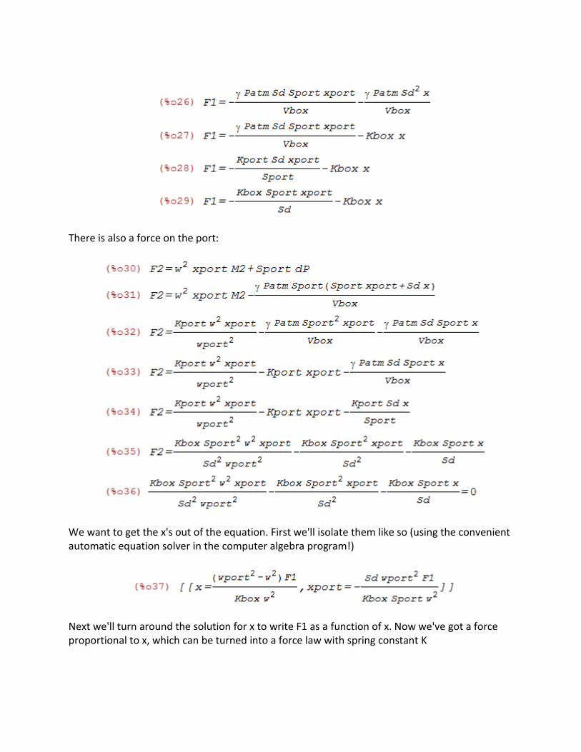
There is also a force on the port:

We want to get the x's out of the equation. First we'll isolate them like so (using the convenient automatic equation solver in the computer algebra program!)

Next we'll turn around the solution for x to write F1 as a function of x. Now we've got a force proportional to x, which can be turned into a force law with spring constant K

This equation shows an obvious factor that completely describes the efffect of the port:

To "use" the port, simply multiply K by the port correction factor which imposes a frequency dependent spring constant on the box.

Looking at (%o39) again, what happens when w = wport? At the port tuning frequency, K goes to infinity, i.e., the box becomes infinitely stiff, and the cone stops moving. Also, a program using this formula will produce a divide-by-zero error. This can’t be real, but it’s a pretty close approximation. In reality, the port probably dissipates some heat, so we can give it a Q factor, for instance:

Assigning an arbitrarily high value to , such as 50, prevents the modeling program from

crashing, and is probably realistic.

Now, looking ahead, the sound produced by the system will be based on the total volume displaced by both the cone and the port. So we find out how much that is.

We correct the displacement of the cone by the same factor that we use to correct the spring constant.

Port air speed

Going back to the relationship between the two port displacements, the speed is simply jw times the displacement (I used x1 instead of velocity):

Effect of coil inductance: Here’s some relief after that heroic battle. Coil inductance is handled by replacing R with a complex value:

Here, L is the coil inductance in Henries, not to be confused with the length of the coil in the BL factor. The cause of coil inductance is that current flowing through the coil causes a slight change in the magnetic field.

System impedance: The general (frequency dependent) version of Ohm’s Law is:

Thus Z can be defined as the voltage-current ratio:

Going all the way back to the beginning, we have an equation containing voltage and current, but not their ratio:

However, we can work with that equation, because we now know that cone velocity v is proportional to the input voltage, and we have a formula for it. Making a small re-write:

( )

(

)

Thus:

Since x is proportional to V, we can use the value of x for a 1-Volt input to compute Z:

( )

Putting it together: My approach to modeling We’ve slogged through a lot of math, and maybe some of us are lost. So it might be nice to take a real breather (get some coffee) and talk about how I do modeling. Doing the math helped me to understand speakers, but it also provides me with the formulas that I can turn into a computer program. And if nothing else, comparing the output of my program to a well-known program such as WinISD will tell me if I got all of it right. The driver: It is a motor driven by a magnet, pushing a cone that’s constrained by the suspension. A balance among several physical laws give the speaker its desired behavior.

Thiele-Small parameters: These are what the industry has chosen as a standard way to report specs. I turn them into more intuitive (for me) electromechanical parameters, such as the mass of the cone and the strength of the magnetic field. I don’t think in terms of those Q’s. The box: It’s a spring, whose stiffness can be adjusted by changing the box volume. Thus it’s a “knob” that can change the overall response curve of the speaker. Hopefully, you start with a driver whose spring constant is insufficient by itself, so that the combined spring constants of the driver and box will end up being something useful. The port: To model the port, I simply let my program generate the graphs, and I look at them. This is where a professional designer might have a more sophisticated approach. Multiple drivers, ports, etc.: I use symmetry to figure out these things, by computing an equivalent box with a single driver and port, and then computing the effect of multiple systems. I use a programming language that handles complex numbers automatically. Here’s how my program works its way through the computations:

Step Formulas

Entry of the Thiele-Small parameters for the chosen drivers, and parameters of the box (volume, port tuning frequency, port area)

Conversion of Thiele-Small parameters into an equivalent set of electromechanical parameters

The “program” given above

Create a table of frequencies, for instance from 25 to 250 Hz. At each frequency…

Compute the effective coil impedance

Compute the effective spring constant Combination of driver and box spring constants, modified by the port correction factor

Compute cone excursion The cone excursion formula, using the modified Z and K values.

Effective displacement Formula for total displacement of cone plus port

SPL Acoustical output formula, using the effective displacement

Port air speed Formula given above

Impedance Formula given above

More References Background reading that I found to be useful

http://www.arcavia.com/kyle/Equations/index.html http://www.silcom.com/~aludwig/ http://www.diysubwoofers.org/

Information that I pulled into this report

http://hyperphysics.phy-astr.gsu.edu/hbase/oscda.html http://www.physics.ox.ac.uk/qubit/tutes/DampedHO.pdf http://www.animations.physics.unsw.edu.au/jw/Adiabatic-expansion-compression.htm