Embed Size (px)
Citation preview
The Prerequsites The Warm-up: Variance Linear Models
How a little linear algebra can go a long wayin the Math Stat course
Randall Pruim
Calvin College
The Prerequsites The Warm-up: Variance Linear Models
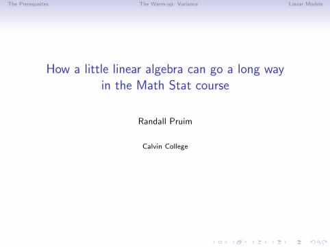
What my students (sort of) know coming in
In theory, my students know
• How to add/subtract vectors; scalar multiplication
• How to represent vectors in Cartesian coordinates(with strong preference for 2d and 3d)
• How to compute a dot product (perhaps matrix multiplication, too)
• The Pythagorean Theorem and how to compute the length(magnitude) of a vector
• u ⊥ v ⇐⇒ u · v = 0
• Perhaps u · v = |u| · |v| cos θ
• How to compute projections using dot products
• The notion of a span
In practice, these need to be refreshed a bit for some of them, but theydo not find this difficult. (I assign a reading and some problems and onlydiscuss difficulties in class.) They get more fluent as we go along.
The Prerequsites The Warm-up: Variance Linear Models
Additional Linear Algebra they need

The Prerequsites The Warm-up: Variance Linear Models
To Sum up . . .
1. Students don’t need a lot of linear algebra to make use of linearalgebra in statistics
2. The review of basic linear algebra in an application area is good fortheir linear algebra
3. (A little) linear algebra provides an important perspective onstatistics
The Prerequsites The Warm-up: Variance Linear Models
Linear Algebra and Statistics (1)
Summary: The expected values and variances of linear combinations ofindependent normal random variables are easily computed.
Example: Suppose X1 ∼ Norm(µ1, σ21), and X2 ∼ Norm(µ2, σ
22).
Then
• E(aX1 + bX2) = aµ1 + bµ2,
• Var(aX1 + bX2) = a2σ21 + b2σ2
2
That is,
• E(〈a, b〉 · 〈X1,X2〉) = 〈a, b〉 · 〈µ1, µ2〉• Var(〈a, b〉 · 〈X1,X2〉) = 〈a2, b2〉 · 〈σ2
1 , σ22〉
Bonus: If the component distributions are normal, the linear combinationis also normal.
Linear algebra provides notation and perspective (and makes it easier toincrease diminesion).
The Prerequsites The Warm-up: Variance Linear Models
Linear Algebra and Statistics (2)
If u ∈ Rn is a constant vector and X = 〈X1,X2, . . . ,Xn〉 is a vector ofindependent random variables with means µ = 〈µ1, µ2, . . . , µn〉 andstandard deviations σ = 〈σ1, σ2, . . . , σn〉, then
1. E(u · X) = u · µ2. Var(u · X) = u2 · σ2
Summary: Linear combinations of independent [normal] random variablesare [normal] random variables with means and variances that are easilycomputed.
The Prerequsites The Warm-up: Variance Linear Models
Linear Algebra and Statistics (2)
If u ∈ Rn is a constant vector and X = 〈X1,X2, . . . ,Xn〉 is a vector ofindependent random variables with means µ = 〈µ1, µ2, . . . , µn〉 andstandard deviations σ = 〈σ1, σ2, . . . , σn〉, then
1. E(u · X) = u · µ2. Var(u · X) = u2 · σ2
In particular, if |u| = 1, and Xiid∼ Norm(µ, σ), then
1. E(u · X) = (u · 1)µ
2. Var(u · X) = (u2 · 1)σ2 = σ2
3. u · X is a normal random variable
And if, in addition, u ⊥ 1, then
1. E(u · X) = 0
Summary: Linear combinations of independent [normal] random variablesare [normal] random variables with means and variances that are easilycomputed. (Note: There are some important special cases.)
The Prerequsites The Warm-up: Variance Linear Models
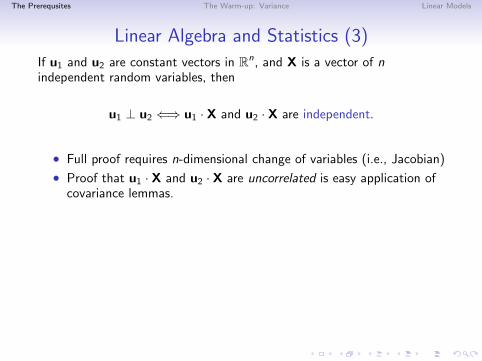
Linear Algebra and Statistics (3)
If u1 and u2 are constant vectors in Rn, and X is a vector of nindependent random variables, then
u1 ⊥ u2 ⇐⇒ u1 · X and u2 · X are independent.
• Full proof requires n-dimensional change of variables (i.e., Jacobian)
• Proof that u1 · X and u2 · X are uncorrelated is easy application ofcovariance lemmas.
The Prerequsites The Warm-up: Variance Linear Models
Looking at variance
The definition of sample variance:
s2 =n∑
i=1
(xi − x)2
n − 1
=|x− x|2
n − 1
mean: x
data: x
variance: x− x
x = proj(x→ 1) , so x− x ⊥ x
(x− x) · x =∑
(xi − x)x = x∑
(xi − x) = x(nx − nx) = 0
The Prerequsites The Warm-up: Variance Linear Models
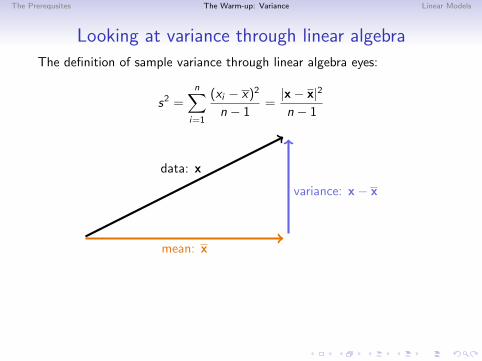
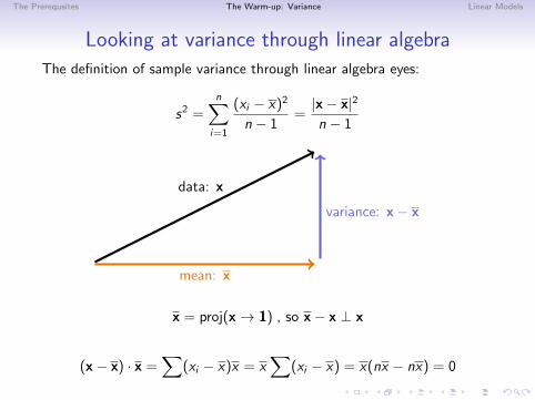
Looking at variance through linear algebra
The definition of sample variance through linear algebra eyes:
s2 =n∑
i=1
(xi − x)2
n − 1
=|x− x|2
n − 1
mean: x
data: x
variance: x− x
x = proj(x→ 1) , so x− x ⊥ x
(x− x) · x =∑
(xi − x)x = x∑
(xi − x) = x(nx − nx) = 0
The Prerequsites The Warm-up: Variance Linear Models
Looking at variance through linear algebra
The definition of sample variance through linear algebra eyes:
s2 =n∑
i=1
(xi − x)2
n − 1=|x− x|2
n − 1
mean: x
data: x
variance: x− x
x = proj(x→ 1) , so x− x ⊥ x
(x− x) · x =∑
(xi − x)x = x∑
(xi − x) = x(nx − nx) = 0
The Prerequsites The Warm-up: Variance Linear Models
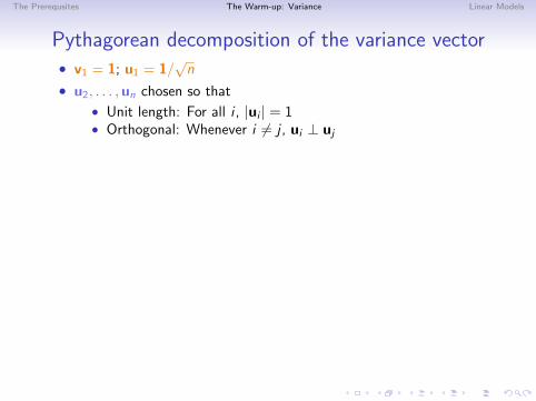
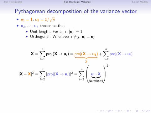
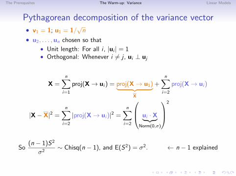
Pythagorean decomposition of the variance vector• v1 = 1; u1 = 1/
√n
• u2, . . . ,un chosen so that
• Unit length: For all i , |ui | = 1• Orthogonal: Whenever i 6= j , ui ⊥ uj
X =n∑
i=1
proj(X→ ui ) = proj(X→ u1)︸ ︷︷ ︸X
+n∑
i=2
proj(X→ ui )
|X− X|2 =n∑
i=2
|proj(X→ ui )|2 =n∑
i=2
ui · X︸ ︷︷ ︸Norm(0,σ)
2
So(n − 1)S2
σ2∼ Chisq(n − 1), and E(S2) = σ2. ← n − 1 explained
The Prerequsites The Warm-up: Variance Linear Models
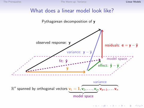
What does a linear model look like?
Pythagorean decomposition of y
model space
y
observed response: y
fit: yeffect: y − y
residuals: e = y − y
variance: y − y
Rn spanned by orthogonal vectors ︸ ︷︷ ︸model space
v1 = 1,
variance︷ ︸︸ ︷v2, . . . , vp, vp+1, . . . vn
Least Squares: Minimizing∑
(yi − yi )2 = |e|2.
The Prerequsites The Warm-up: Variance Linear Models
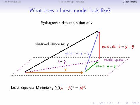
What does a linear model look like?
Pythagorean decomposition of y
model space
y
observed response: y
fit: yeffect: y − y
residuals: e = y − y
variance: y − y
Least Squares: Minimizing∑
(yi − yi )2 = |e|2.
The Prerequsites The Warm-up: Variance Linear Models
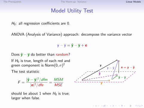
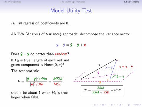
Model Utility Test
H0: all regression coefficients are 0.
ANOVA (Analysis of Variance) approach: decompose the variance vector
y − y = y − y + e
Does y − y do better than random?
If H0 is true, length of each red andgreen component is Norm(0, σ)2
The test statistic
F =|y − y|2/dfm|e|2/dfe
=MSM
MSE
should be about 1 when H0 is true;larger when false.
y
y
yy − y
e = y − yy − y
R2 =SSM
SSM + SSE= cos θ
The Prerequsites The Warm-up: Variance Linear Models
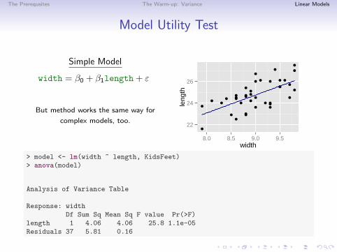
Model Utility Test
Simple Model
width = β0 + β1length + ε
But method works the same way for
complex models, too.
22
24
26
8.0 8.5 9.0 9.5width
leng
th
> model <- lm(width ~ length, KidsFeet)> anova(model)
Analysis of Variance Table
Response: widthDf Sum Sq Mean Sq F value Pr(>F)
length 1 4.06 4.06 25.8 1.1e-05Residuals 37 5.81 0.16
The Prerequsites The Warm-up: Variance Linear Models
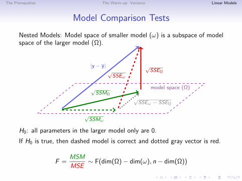
Model Comparison Tests
Nested Models: Model space of smaller model (ω) is a subspace of modelspace of the larger model (Ω).
model space (Ω)
√SSMω
√SSEω − SSEΩ
√SSMΩ
√SSEΩ√
SSEω
|y − y|
H0: all parameters in the larger model only are 0.
If H0 is true, then dashed model is correct and dotted gray vector is red.
F =MSM
MSE∼ F(dim(Ω)− dim(ω), n − dim(Ω))
The Prerequsites The Warm-up: Variance Linear Models
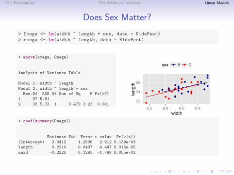
Does Sex Matter?
> Omega <- lm(width ~ length + sex, data = KidsFeet)> omega <- lm(width ~ length, data = KidsFeet)
> anova(omega, Omega)
Analysis of Variance Table
Model 1: width ~ lengthModel 2: width ~ length + sex
Res.Df RSS Df Sum of Sq F Pr(>F)1 37 5.812 36 5.33 1 0.479 3.23 0.081
22
24
26
8.0 8.5 9.0 9.5width
len
gth
sex B G
> coef(summary(Omega))
Estimate Std. Error t value Pr(>|t|)(Intercept) 3.6412 1.2506 2.912 6.139e-03length 0.2210 0.0497 4.447 8.015e-05sexG -0.2325 0.1293 -1.798 8.055e-02
The Prerequsites The Warm-up: Variance Linear Models
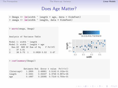
Does Age Matter?
> Omega <- lm(width ~ length + age, data = KidsFeet)> omega <- lm(width ~ length, data = KidsFeet)
> anova(omega, Omega)
Analysis of Variance Table
Model 1: width ~ lengthModel 2: width ~ length + age
Res.Df RSS Df Sum of Sq F Pr(>F)1 37 5.812 36 5.73 1 0.0829 0.52 0.47
22
24
26
8.0 8.5 9.0 9.5width
len
gth
11.111.411.712.012.3age
> coef(summary(Omega))
Estimate Std. Error t value Pr(>|t|)(Intercept) 1.2855 2.49981 0.5142 6.102e-01length 0.2331 0.05327 4.3746 9.967e-05age 0.1667 0.23085 0.7219 4.750e-01
The Prerequsites The Warm-up: Variance Linear Models
To sum up . . .
1. Students don’t need a lot of linear algebra to make use of linearalgebra in statistics
2. The review of basic linear algebra in an application area is good fortheir linear algebra
3. (A little) linear algebra provides an important perspective onstatistics
The Prerequsites The Warm-up: Variance Linear Models
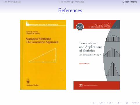
References
!"#$%&'("$)*&$%*+,,-(.&'("$)*"/*0'&'()'(.)+$*1$'2"%#.'("$*3)($4*!
!"#$"%%&'()*+
+562(.&$*7&'865&'(.&-*0".(6'9
!"#$%&'("$)*&$%*+
,,-(.&'("$)*"/*0'&'()'(.)***'
()*+
,-./!0!1.,12/&&&&&&2/324
154
&&&&&&&267&!"##$&&&&&4/!8/4
%&'()"*+),--#.(+9:
1542/32
9:
154&;#&<67&=7>&&???@"+A@;(B+70:;<:=>?
!"2*&%%('("$&-*($/"25&'("$*&$%*#,%&'6)*"$*'8()*@""AB*C()('
???@"+A@;(BC>;;DE"B7AC"+A<7F<G9:
2-color cover: PMS 432 (Gray) and PMS 1805 (Red) ??? pages • Backspace 1 1/8" • Trim Size: 7" x 10"
&&&&&&&267&!"##$&&&&&4/!8/4
!is series was founded by the highly respectedmathematician and educator, Paul J. Sally, Jr.