Embed Size (px)
Citation preview

Housing Supply Elasticity and Rent Extraction by
State and Local Governments
Rebecca Diamond�
November 7, 2012
Abstract
It is possible government workers can extract rent from private sector workers bycharging high tax rates and paying themselves high wages. Using a spatial equilibriummodel where private sector workers are free to migrate across government jurisdictions,I show that private sector workers�migration elasticity with respect to local taxes de-termines the magnitude of rent extraction by rent seeking state and local governments.Since private sector workers �vote with their feet�by migrating out of rent extractiveareas, governments trade o¤ the bene�ts a higher tax rate with the cost of a smallerpopulation to tax. Variation in areas�housing supply elasticities di¤erentially restrainsgovernments�abilities to extract rent from private sector workers. The incidence of atax increase falls more on local housing prices in a less housing elastic area, leading toless out-migration. Thus, governments in less housing elastic areas can charge highertaxes without worry of shrinking their tax bases. I test the model�s predictions byusing worker wage data from the CPS-MORG. I �nd the public-private sector wagegap is higher in areas with less elastic housing supplies. This fact holds both withinstate across metropolitan areas for local government workers and between states forstate government workers.
�I am very grateful to my advisors Edward Glaeser, Lawrence Katz, and Ariel Pakes for their guidance andsupport. I also thank Nikhil Agarwal, Adam Guren, and participants at the Harvard Labor and IndustrialOrganization Workshops. I acknowledge support from a National Science Foundation Graduate ResearchFellowship.
1

1 Introduction
Can government workers extract rent from private sector workers by charging high tax rates
and paying themselves high wages? The determinants and justi�cation of government work-
ers�compensation levels has taken on considerable heat in the past few years, as many states
and localities face budgetary stress. Since state and local governments set taxes and govern-
ment employee wages, government employees could earn rents by charging high taxes and
receiving high wages. There has long been debate over whether the government acts as a
benevolent social planner for its citizens or uses its market power to bene�t its workers and
political interest groups. (See Gregory and Borland (1999) for a review of this literature.)
In particular, the high unionization rate in the public sector may allow union bargaining
to in�uence the political process and the decisions of elected o¢ cials (Freeman (1986)). In
this paper, I analyze whether government workers receive higher wages than similar private
sector workers in areas where state and local governments have stronger abilities to exercise
market power.
This paper develops a model where state and local governments set taxes and the level of
government services to maximize government "pro�ts", which can then be paid to employees
as excessive wages. I use a Rosen (1979) Roback (1982) spatial equilibrium model where
workers maximize their utility by living in the city which o¤ers them the most utility based
on the city�s wage, rental rate of housing, tax rate, government services, and other amenities.
Thus, governments must compete for residents to tax, and workers can "vote with their feet"
by migrating away from excessively rent extractive governments.
I show that if state and local governments are using their market power to over pay their
employees, their abilities to extract rents from their citizens is determined by the equilibrium
migration elasticity of private sector residents with respect to local tax rates. Governments
must trade o¤ the bene�ts of a higher tax with the cost that a higher tax will cause workers
to migrate away, leaving the government with a smaller population to tax. This is analogous
to the standard result found in analysis of imperfect competition between product producers
2

where a �rm�s optimal price markup over cost is equal to the inverse elasticity of consumer
demand with respect to price for the �rm�s product.
Unlike �rm competition for consumer demand, I show that a government�s market power
to charge wasteful taxes remains even when there are a large number of governments com-
peting for residents and every government is small.1 The spatial equilibrium model shows
that when a government raises taxes, workers will migrate away to other jurisdictions. How-
ever, this out-migration decreases the level of labor supply and housing demand in the area.
Assuming labor demand curves slope down and housing supply curves slope up, this decrease
in population raises wages and decreases housing rents. Thus, some of the disutility of a tax
increase will be o¤set by an increase in the desirability of local wages and rents, which limits
the amount of out-migration caused by the tax increase. Since the local housing and labor
markets will respond to government imposed taxes through migration, the government will
always have market power.
An area�s elasticity of housing supply will determine how local housing rents respond
to population changes in an area. Governments presiding over areas with inelastic housing
supplies will have more market power than governments in housing elastic areas. A tax
hike by a government in an area with inelastic housing supply leads to a small amount of
out-migration because housing prices sharply fall due to the decrease in housing demand
driven by the tax hike. The housing cost decline o¤sets the negative utility impact of a
tax increase with a only small amount of out-migration in the housing inelastic area. Thus,
governments in housing inelastic areas can charge higher taxes without shrinking their tax
base since housing price changes limit the migration response.
If state and local governments exercise more market power in areas with inelastic housing
supplies, the wage gap between public and private sectors workers should be larger in these
areas. I test the model�s prediction by measuring variation in public-private sector wage
gaps across areas with di¤erent housing supply elasticities. I measure workers�wages using
1This result is closely related to Epple and Zelenitz (1981), which shows that worker migration betweengovernment juristidictions is not enough to entirely compete away a government�s market power.
3

data from the 1995-2011 Current Population Survey Merged Outgoing Rotation Groups
(CPS-MORG). I proxy for a metropolitan areas�s housing supply elasticity using data from
Saiz (2010) on the share of land within 50km of a city�s center unavailable for real-estate
development due to geographic constraints, such as the presence of swamps, steep grades,
or bodies of water. With less available land around to build on, the city must expand
farther away from the central business area to accommodate a given amount of population,
driving up average housing costs.2 I also use the Wharton Land Use Regulation Index
from Gyourko, Saiz, and Summers (2008) as component of housing supply elasticity. Since
the decision to regulate real-estate development is endogenous and possibly correlated with
unobserved characteristics which could impact government workers wages, I focus on the
Saiz (2010) measure of geographic constraints on real-estate development as an exogenous
source of variation in housing supply elasticity. These data are the metropolitan area level.
To measure states�housing supply elasticities I use an average of these measures across each
state�s MSAs, weighted by the MSAs�populations.
I �nd that the public-private sector wage gap is higher in states and metropolitan ar-
eas with less elastic housing supplies. This result holds when analyzing variation in state
government-private sector wage gaps across states and in local government-private sector
wage gaps across MSAs. This �nding is robust to including a host of controls for workers�
demographics and characteristics, including dummies for three digit occupation codes. Ad-
ditionally, the local government-private sector wage gap is found to be higher in housing
inelastic MSAs, even when only comparing MSAs within the same state.
As falsi�cation tests, I show that housing supply elasticity has no impact on the federal
government worker-private sector wage gap. Since federal workers� compensation is not
2A full micro-foundation of this mechanism can be derived from the Alonso-Muth-Mills model (Brueckner(1987)) where housing expands around a city�s central business district and workers must commute fromtheir house to the city center to work. Within-city house prices are set such that workers are indi¤erentbetween having a shorter versus longer commute to work. Average housing prices rise as the populationgrows since the houses on the edge of the city must o¤er the same utility as the houses closer in. As thecity population expands, the edge of the city becomes farther away from the center, making the commutingcosts of workers living on the edge higher than those in a smaller city. Since the edge of the city must o¤erthe same utility value as the center of the city, housing prices rise in the interior parts of the city.
4
derived from government revenues of their place of residence, the market power of the state
and local government should have no impact on their wages. Additionally, I show that
variation in the state government worker-private sector wage gap does not vary across MSAs,
within a state. The public-private wage gaps only vary with housing supply elasticities when
the housing supply elasticity variation impacts the government�s market power. I also show
that the e¤ect is larger for government workers who are union members, suggesting unions
allow government workers to bargain for a larger share of government rents.
The CPS-MORG only reports data on workers�earnings, and does not include data on
the value of workers�benefts. Gittleman and Pierce (2012) show that goverment employees
receive more generous bene�ts than similar private sector workers, on average. I use data
from on average government pension payouts per bene�ciary across states from the Census�
2007-2010 Annual Surveys of Public Employee Retirement Systems as a measure of state
government workers�bene�ts. While I do not have a data source for similar private sector
workers�retirement bene�ts, I show that average annual state government pension payouts
per bene�ciary are higher in states with less elastic housing supplies. This suggests that the
wage gap estimates from the CPS understate the full impact of housing supply elasticity on
government worker compensation.
Previous work has also found evidence suggesting government jobs are more desirable
than similar private sector jobs. Gittleman and Pierce (2012) show that public sector em-
ployees are more generously compensated than similarly quali�ed private sector employees.
In particular, they �nd that government worker wages tend to be slightly lower than similar
private sector workers. However, the value of government workers�bene�ts strongly outweigh
those of the private sector, leading to public sector employees to be better compensated over-
all. Krueger (1988) �nds that there are more job applications for each government job than
for each private sector job, suggesting that government jobs are more desirable to workers,
on average. Additionally, average job quit rates reported from the 2002-2006 Job Openings
and Labor Turnover Surveys show that average annual quit rate is 28% for private sector
5

workers, but only 8% for public sector employees. These fact taken together suggest that
government jobs are better compensated than private sector jobs, and that there appears to
be excess labor supply for these jobs, which is consistent with government workers receiving
rents. While this evidence shows that government jobs appear desirable to workers, it is not
clear that this desirability is due to rent-seeking behavior of governments exercising market
power. My paper shows that an increase in governments�abilities to extract rent directly
leads to better paid government employees.
The public sector workforce is also highly unionized, enabling government employees to
bargain for government rents. Gyourko and Tracy (1991) use a spatial equilibrium model to
show that if the cost of government taxes to citizens are not completely o¤set by bene�ts
of government services, they will be capitalized into housing prices. Similarly, if high levels
of public sector unionization lead to more government rent extraction, the public sector
unionization rate will proxy for government waste and also be capitalized into housing prices.
While Gyourko and Tracy (1991) �nd evidence for both of these e¤ects, it is unclear what
drives the variation in taxes and unionization rates across localities. This paper uses housing
supply elasticity as a source of exogenous variation in government market power to assess
whether government take advantage of their power to over pay employees.
Brueckner and Neumark (2011) considers whether government can extract more rent from
local residents if the government presides over an area with more desirable amenities. They
use a similar setup to this paper where pro�t maximizing governments compete for residents
by setting local tax rates. They allow local governments to play a game in tax-competition
where the number of competing governments is small. My model di¤ers from theirs by
allowing each government to be small when deriving tax rates chosen by governments. They
�nd evidence that amenity di¤erences are positively associated with public-private wage
gaps. However, it is possible that some of the amenity measures, such as coastal proximity
and population density, are correlated with housing supply elasticity di¤erences.
The paper proceeds as follows. Section 2 layouts of the model. Section 3 presents
6
empirical evidence, and Section 4 concludes.
2 Model
The model detailed below uses a Rosen (1979) Roback (1982) spatial equilibrium to analyzes
how local governments set taxes and compete for residents. In the model, I assume that
governments use a head tax to collect revenue, however in reality, most state and local
governments use property and income tax instruments. In Appendix A I derive results for
the case of a government income or property tax and show the same results. I also abstract
away from the political election process in each area. While politics could surely in�uence
the extent of government rent seeking, my goal is to analyze contributors to governments�
abilities to excercise market power if they had a rent seeking motivation.
The nationwide economy is made up of many cities. There are N cities, where N is large.
Cities are di¤erentiated by their endowed amenity levels Aj;which impact how desirable
workers �nd the city, and their endowed productivity levels �j; which impact how productive
�rms are in the city. Workers are free to migrate to any city within the country. Each city
has a local labor and housing market, which determine local wages and rents. The local
government provides government services and collects taxes.
2.1 Government
The local government of city j charges a head tax � j to workers who choose to reside within
the city. The local government also produces government services, which cost sj for each
worker in the city. The government revenue and cost are
Revenuej = � jNj
Costj = sjNj:
7

Nj measure the population of city j: The local government is not benevolent and maximizes
pro�ts. These pro�ts could be spent on ine¢ cient production of sj (thus, making the
government benevolent, but naive). They could also be directly pocketed by government
workers, such as through union negotiations. The local government maximizes:
max�j ;sj
� jNj � sjNj
2.2 Workers
All workers are homogeneous. Workers living in city j inelastically supply one unit of labor,
and earn wage wj: Each worker must rent a house to live in the city at rental rate rj and
pay the local tax � j:Workers value the local amenities as measure by Aj:The desirability of
government services sj is represented by g (sj) : Thus, workers�utility from living in city j
is:
Uj = wj � rj + Aj + g (sj)� � j:
Workers maximize their utility by living in the city which they �nd the most desirable.
2.3 Firms
All �rms are homogenous and produce a tradeable output Y:Cities exogenously di¤er in
their productivity as measured by �j. Local government services impact �rms productivity,
as measured by b(sj): The production function is:
Yj = �jNj + b(sj)Nj + F (Nj) ;
where F 0 (Nj) > 0 and F 00 (Nj) < 0 in labor:
The labor market is perfectly competitive, so wages equal the marginal product of labor:
wj = �j + b(sj) + F0 (Nj) :
8

2.4 Housing
Housing is produced using construction materials and land. All houses are identical. Houses
are sold at the marginal cost of production to absentee landlords, who rents housing to
the residents. The asset market is in long-run steady state equilibrium, making housing
price equal the present discounted value of rents. Housing supply elasticities di¤er across
cities. Di¤erences in housing supply elasticity are due to topography and land use regulation,
which makes the marginal cost of building an additional house more responsive to population
changes (Saiz (2010)). The housing supply curve is:
rj = aj + j log (Nj) ;
j = xhousej
where xhousej is a vector of city characteristics which impact the elasticity of housing supply.
2.5 Equilibrium in Labor and Housing
Since all workers are identical, all cities with positive population must o¤er equal utility to
workers. In equilibrium, all workers must be indi¤erent between all cities. Thus:
Uj = wj � rj + Aj + g (sj)� � j = �U:
Plugging in labor demand and housing supply gives:
�j + b(sj) + F0 (Nj)� aj � j logNj + Aj + g (sj)� � j = �U: (1)
Equation (7) determines the equilibrium distribution of workers across cities.
9

2.6 Government Tax Competition
Local governments set city tax rates and the level of government services to maximize pro�ts,
taking into account the endogenous response of workers and �rms in equilibrium, equation
(7). Each city is assumed to be small, meaning out-migration of workers to other cities does
not impact other cities�equilibrium wages and rents. If there were a small number of cities,
each city would have even more market power than in this limiting case. The results below
can be thought of as a lower bound on the market power of local governments competing for
residents. They maximize:
maxsj ;�j
� jNj � sjNj:
The �rst order conditions are:
0 = � j@Nj@sj
�Nj � sj@Nj@sj
(2)
0 = � j@Nj@� j
+Nj � sj@Nj@� j
:
Di¤erentiating equation (7) to solve for @Nj@sj
and @Nj@�jgives:
@Nj@sj
=b0 (sj) + g
0 (sj)� jNj� F 00 (Nj)
� > 0@Nj@� j
=�1�
jNj� F 00 (Nj)
� < 0: (3)
Population increases with government services and decreases in taxes. Plugging these into
(8) gives:
0 = (� j � sj)
0@ b0 (sj) + g0 (sj)�
jNj� F 00 (Nj)
�1A�Nj
� j = Nj
� jNj� F 00 (Nj)
�+ sj:
10

Combining the �rst order conditions shows that government services are provided such that
the marginal bene�t (b0 (sj) + g0 (sj)) equals marginal cost (1) :
b0�s�j�+ g0
�s�j�= 1:
This is the socially optimal level of government service.
The equilibrium tax rate is:
� �j = j �NjF 00 (Nj) + s�j : (4)
The elasticity of city population with respect to the tax rate�"migratej
�can be written as:
"migratej =@Nj@� j
� jNj:
Plugging in equation (9) for @Nj@�j
and rearranging gives:
� jNj� F 0 (Nj)
�Nj =
�� j"migratej
:
Substituting this expression into the equation (10) shows that the tax markup can be written
as:� �j � s�j� �j
=�1
"migratej
:
The tax markup above cost is equal to the inverse elasticity of city population with respect
to the tax rate: While workers are perfectly mobile between cities, worker migration causes
shifts along the local labor demand and housing supply curves. An increase in local taxes
would cause workers to migrate to other cities. A decrease in population will increase local
wages, since I have assumed a downward sloping labor demand curve. The decrease in
population will also cause rents to fall, by moving along the housing supply curve. This
increase in wages and decrease in rents will increase the desirability of the city to workers,
11
limiting the migration response to the tax increase. The government takes into account the
equilibrium wage and rent response to a tax hike when setting taxes to pro�t maximize.
Thus, if migration leads to large changes in local wages and rent, a tax increase will not lead
to large amounts of out-migration, since workers will be compensated for the tax with more
desirable wages and rents.
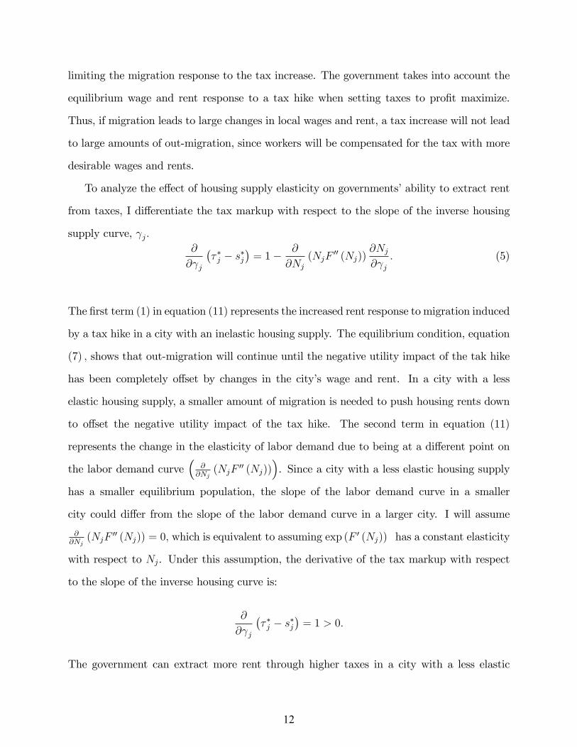
To analyze the e¤ect of housing supply elasticity on governments�ability to extract rent
from taxes, I di¤erentiate the tax markup with respect to the slope of the inverse housing
supply curve, j:@
@ j
�� �j � s�j
�= 1� @
@Nj(NjF
00 (Nj))@Nj@ j
: (5)
The �rst term (1) in equation (11) represents the increased rent response to migration induced
by a tax hike in a city with an inelastic housing supply. The equilibrium condition, equation
(7) ; shows that out-migration will continue until the negative utility impact of the tak hike
has been completely o¤set by changes in the city�s wage and rent. In a city with a less
elastic housing supply, a smaller amount of migration is needed to push housing rents down
to o¤set the negative utility impact of the tax hike. The second term in equation (11)
represents the change in the elasticity of labor demand due to being at a di¤erent point on
the labor demand curve�
@@Nj
(NjF00 (Nj))
�. Since a city with a less elastic housing supply
has a smaller equilibrium population, the slope of the labor demand curve in a smaller
city could di¤er from the slope of the labor demand curve in a larger city. I will assume
@@Nj
(NjF00 (Nj)) = 0; which is equivalent to assuming exp (F 0 (Nj)) has a constant elasticity
with respect to Nj. Under this assumption, the derivative of the tax markup with respect
to the slope of the inverse housing curve is:
@
@ j
�� �j � s�j
�= 1 > 0:
The government can extract more rent through higher taxes in a city with a less elastic
12

housing supply.
Note that this result assumes there are a large number of cities. When there are a small
number of cities, the incentives for rent extraction will be even higher. Outward migration
from a city in response to a tax increase will lead to increases in other cities� rents and
decreases in their wages, leading to less outward migration in response to tax increases. I
have assumed this e¤ect away by not allowing the equilibrium utility level across all cities to
fall in response to a given city�s tax increase. Cities can extract rent even in an environment
where there are a large number of competitors because household demand for city residence
can never be in�nite in equilibrium.
Additionally, this model assumes cities charge a head tax, while in reality most cities and
states tax their population through income taxes and property taxes. The amount of rent
extraction depends on the elasticity of tax revenue with respect to the tax rate. Thus, an
income tax will depend both on the wage response to the tax rate, as well as the migration
response. Appendix A shows that when using an income tax, governments can still excercise
more market power in housing inelastic areas.
In the case of a property tax, government revenue will depend on local the rental rate
and the size of the tax base. An increase in the property tax rate can decrease government
revenue both by incentivizing workers to migrate away, shrinking the tax base, and decreasing
housing rents, lowering tax revenue from each household. However, I show in appendix A
that if local labor demand is perfectly elastic, the housing supply elasticity will not impact
the size of the rental rate decrease in response to a given tax hike. To see this, recall the
equilibrium condition, equation (7) : For workers to derive utility �U from a local area, the
utility impact of a tax increase must be perfectly o¤set by a rent decrease, if labor demand
is perfectly elastic. Thus, the equilibrium rental rate response to a given tax increase does
not depend on the local housing supply elasticity. Indeed, the housing supply elasticity
determines the migration response required to change housing rents in order to o¤set the
utility impact of the tax increase. Thus, a less elastic housing supply decreases the elasticity
13

of government revenue with respect to the tax rate, giving the government more market
power when using a property tax instrument. See Appendix A for the full derivation of this
result.
Regardless of the tax instrument, governments of cities with less elastic housing supplies
are able to extract more rent from their residents. In the next section, I empirically test this
prediction.
3 Empirical Evidence
The model predicts that local governments in areas with less elastic housing supplies will be
able to extract more rent from their residents. While this extra money could be spent in a
number of ways, it is likely that some of it gets absorbed into public sector workers�wages.
Since most public sector workers are unionized, they will be able to bargain to gain some
of these rents as wages. Thus, the wage gap between government employees and similarly
quali�ed private sector workers should be higher in areas with less elastic housing supplies.
The e¤ect should hold across metropolitan areas for local government-private sector wage
gaps and across states for state government-private sector wage gaps.
To test this, I estimate how states�and MSAs�public/private sector wage gaps vary with
characteristics which impact local housing supply elasticities. Saiz (2010) shows that the
topological characteristics of land around an MSA�s center impact whether the land can
used for real-estate development. Cities located next to wetlands, bodies of waters, swamps,
or extreme hilliness have limits on how many building can be built close to the city center,
which impacts the elasticity of housing supply to the area. Saiz (2010) uses satellite data to
measure the share of land within 50km of an MSA�s center which cannot be developed due
to these topological constraints. A rent-seeking government is able to charge higher taxes
in areas with less land available for development. Thus, the public-private sector wage gap
should be higher in these areas.
14

A city�s housing supply elasticity is also in�uenced by the amount of land-use regulation
in the area. The 2005 Wharton Land Use Regulation Survey Gyourko, Saiz, and Summers
(2008) collected survey data on a number of land-use regulations and practices, which were
aggregated into the Wharton Land Use Regulation Index (WLURI). Saiz (2010) aggregates
this municipality measure into a MSA-level index.
I z-score the MSA level data from the WLURI and the land unavailability measure and
will use both as measures of cities�housing supply elasticities. I also aggregate these measures
to a state-level index, where I weight each MSA measure by the state population in each
MSA. The state-level housing supply elasticity measure is a noisy measure of the overall
housing supply elasticity for the state, since the data is only based o¤ of the MSAs covered
by Saiz�s sample. Table 1 reports summary statistics on these measures. The data covers 48
states (there is no data for Hawaii or Alaska) and 228 MSAs.
3.1 Wage Gap Regressions
To measure public-private sector wage gaps across MSAs and states, I use data from the
Current Population Survey Merged Outing Rotation groups from 1995-2011.3 The CPS-
MORG is a household survey which collects data on a large number of outcomes including
workers�weekly earnings, hours worked, public/private sector of employment, union status,
and a host of demographics. I restrict the sample to 25 to 55 year old workers with positive
labor income, working at least 35 hours per week, to have a standardized measure of weekly
earnings. The CPS�s usual weekly earnings question does not include the self-employment
income so all analysis excludes the self-employed. I also restrict analysis to workers whose
wages are not imputed to avoid any bias due to the CPS�s wage imputation algorithm
(Bollinger and Hirsch (2006)). I measure earnings using workers�log usual weekly earnings,
3Since there was a signi�cant change in the CPS�s earnings questions in 1994, I restrict analysis to 1994-2011. I also focus my analysis on workers whose wages are not imputed in the CPS. Since sector, occupation,and union status and not used in the CPS�s imputation algorithm, analyzing government wage gaps andunion wage gaps using imputed wages can be problematic (Bollinger and Hirsch (2006)). Thus, I focus onlyon the non-imputed wage sample. The data �agging which wages were imputed are missing in the 1994 data,so I drop this year, leaving me with a 1995-2011 sample.
15

de�ated by the CPI-U and measured in real 2011 dollars. Top coded weekly earnings are
multiplied by 1.5 and weekly earnings below $128 are dropped from the analysis.4 All analysis
is weighted by the CPS earnings weights.
Table 1 reports summary statistics of workers� log weekly earnings each for workers
employed in the private sector, local government, state government, and federal government.5
Consistent with previous works, such as Gittleman and Pierce (2012), the raw earnings are
higher for all three classes of government workers than for private sector workers. However,
these raw earnings di¤erences do not account for di¤erences in the characteristics of workers
between the public and private sector. To test the model�s predictions, I will control for
worker characteristics when evaluating di¤erences in the public private sector wage gap.
Additionally, the CPS only collects data on workers�earnings, but not compensation paid to
workers in the form of bene�ts. Gittleman and Pierce (2012) show using the BLS�restricted-
use Employer Cost of Employee Compensation microdata that government employees receive
signi�cantly more generous bene�ts than similar workers in the private sector. I will return
to the question of bene�ts compensation, but �rst focus on public-private sector wage gaps.
To test the model�s predictions, I estimate the following regression:
lnwijt = �j + �t + �govgovit + �
elastzelastj � govit + �Xit + "ijt: (6)
As controls, I include location �xed-e¤ects �j; year �xed e¤ects, �t; and a set of worker
demographics which include 15 dummies for education categories, gender, race, Hispanic
origin, a quartic in age, and a rural dummy. govi is a dummy for whether the worker is
government worker, zelastj measures land use regulation and topography. Standard errors are
clustered by state when using state-level measures of housing supply elasticity and clustered
by MSA when using MSA variation in housing supply elasticity.
4I follow Autor, Katz, and Kearney (2008)�s top and bottom coding procedures. Autor, Katz, andKearney (2008) drops all reported hourly wages below $2.80 in real 2000 dollars. This translates to $128 perweek in real 2011 dollars, assuming a 35 hour work week. They also scale top coded wages by 1.5.
5A worker�s sector is measured by the CPS variable reporting a worker�s class.
16

The nationwide average public-private wage gap is measured by �gov:The model predicts
that public-private wage gap should be higher in areas with less elastic housing supplies:
�elast > 0:
The prediction should hold both for areas with less land available for development and for
areas with stricter land-use regulations. Since land-use regulations are chosen by local mu-
nicipalities, it is possible that the decision to regulate land-use could be correlated with other
characteristics of the area which could impact workers�wages. Since the topological con-
straints around a city are pre-determined, they are likely a measure of exogenous di¤erences
in housing supply elasticities across areas. I perform all analysis using both measures, but I
also drop the regulation index to focus directly on the impact of land availability, which is
likely a cleaner estimate of the impact of housing supply elasticity on public-private sector
wage gaps.
I test this prediction �rst using a sample including private sector workers and state gov-
ernment workers. Column 1 of Table 2 shows that the nationwide average wage gap between
state government employees and private sector workers is -0.112 log points. Consistent with
Gittleman and Pierce (2012), after controlling for worker demographics, government work-
ers�earnings are lower than similar private sector workers, on average. However, the state
worker-private sector wage gap increases by 0.017 log points in states with a 1 standard
deviation increase in land unavailability. This e¤ect is signi�cant at the 10% level. The
wage gap is 0.026 log points higher in states with a 1 standard deviation increase land-use
regulation. This e¤ect is signi�cant at the 5% level. In a regression which drops the land-use
index, a 1 standard deviation increase in a state�s land availability increases the wage gap
by 0.026 log points. This e¤ect is signi�cant at the 1% level. Figure 1 plots states� land
unavailability against states�state government worker-private sector wage gaps, after wages
have been residualized against the set of controls included in equation (6) : Figure 1 shows
17

the state government-private sector wage gaps are higher in states including California, Ver-
mont, Florida, and Connecticut, but must lower in states such as Iowa, Texas, Montana,
and Kentucky which lines up with these states�land unavailability. Note that states such as
Utah are signi�cant outliers. However, Utah�s land availability was measured only based on
Salt Lake City, which has a large share of land unavailable for development due proximity
to the Great Salt Lake. This is likely a poor measure of the overall state housing supply
elasticity. Despite the short comings of the state-level data, I �nd that states with less elastic
housing supplies have signi�cantly better paid state government employees, as compared to
the private sector employees residing in the state.
Performing the same analysis on local government employees, I compare the wage gaps
between local government workers and private sector workers across 229 MSAs. The controls
in this setup now include MSA �xed e¤ects and the housing supply measures are now at the
MSA level. Column 3 of Table 2 shows that the nationwide local government worker-private
sector wage gap is -0.080 log points. A 1 standard deviation increase in land unavailability
increases the wage gap by 0.029 log points and a 1 standard deviation increase in land-use
regulation increases the wage gap by 0.0348 log points. Both of these e¤ects are signi�cant at
the 1% level. Dropping the land-use regulation, I �nd the coe¢ cient on land unavailability
increases to 0.037 log points, and is signi�cant at the 1% level. Figure 2 plots MSAs�land
unavailability against MSAs�local government worker-private sector wage gaps, after wages
have been residualized against the set of controls included in equation (6) : The plot shows
high local government wages gaps in land unavailable cities including Los Angeles, New York,
Cleveland, Chicago, and Portland and low government wage gaps in cities with lots of land
to develop including Atlanta, Houston, Minneapolis, and Phoenix. Housing supply elasticity
explains a signi�cant amount of the cross-section variation in public-private wage gaps.
To test whether the local housing supply elasticity measures impact local government
worker-private sector wage gaps within states, across MSAs, I add controls for state di¤er-
18

ences in the local government worker-private sector wage gaps. I now estimate:
lnwijkt = �j + �t + �govgovit + �
govk govit + �
elastzelastj � govit + �Xit + "ijt;
where j represents an MSA and k represents a state. Columns 5 and 6 of Table 2 show
that the impact of land unavailability on the local government-private sector wage gap falls
slightly, but remains statistically sigin�cant when land-use regulations are not included in
the regression. Land unavailability consistently has a positive impact the public-private
sector wage gap both for local and state government workers, as predicted by the model.
Table 3 repeats the analysis adding in dummies for each three-digit occupation code to
attempt to further control for di¤erences in workers�skills in the public and private sectors.
The point estimate measuring the impact of land unavailability of the state government-
private sector wage gap remains positive, but the standard errors increase, making the e¤ect
only statistically signi�cant when land-use regulations are dropped from the regression. How-
ever, the large standard errors shows that one cannot rule out a point estimate equal to the
magnitude found when 3-digit occupation code dummies were not included in the regression.
The estimates for local-government worker wage gaps are positive and statistically sig-
ni�cant at the 1% level. Column 4 of Table 3 shows that even when including the full set of
3 digit occupation dummies, a 1 standard deviation increase in land unavailability increases
the local public-private sector wage gap by 0.028 log points. Note that with the inclusion
of occupation dummies, the nationwide local government worker-private sector wage gap is
now positive and equal to 0.028 log points.
One possible way government workers are able to raise their wages is through union wage
bargaining. I repeat the analysis adding in additional housing supply elasticity interactions
terms for whether the government worker is part of a labor union. I control for the direct
e¤ect of being in a union, and its interaction with the housing supply elasticity characteristics.
This controls for di¤erences in union bargaining power across states and MSAs for all unions,
19

public and private. Table 4 shows that a standard deviation increase in land unavailability
raises state government-private sector wage gaps by 0.0127 log points for non-union members
and an addition 0.0214 log points for unionized government workers. State government
worker unions appear to be able to bargain for better wages in housing inelastic areas,
relative to non-unionized government workers. The point estimates in Columns 3 and 4 of
Table 4 are similar for local government-private sector wage gaps. However, the additional
impact of goverment labor unions is positive, but not statistically signi�cant. These point
estimates suggest government workers part of a labor union might be able to use their market
power to negotiate for a larger amount of excess wages beyond the o¤erings of the private
sector.
Table 5 repeats the analysis separately for workers with and without a 4 year college
education. I �nd a positive and statistically signi�cant e¤ect both for college and non-
college educated workers. The impact of land unavailability is stronger for low skill workers
than for those with a college education. Overall, housing supply elasticity appears to impact
the public-private wage gap.
3.2 Falsi�cation Tests
The evidence presented thus far suggests that governments are exercising their market power
by extracting rents and paying government employees higher wages than are paid by local
private sector employers. Variation in housing supply elasticities across areas impacts the
extent to which governments can exercise market power. A falsi�cation test of these pre-
dictions is to analyze whether the federal government-private sector wage gaps across cities
and states exhibit similar properties. Since federal workers are not paid by the state or local
government which presides over their location of residence, housing supply elasticity should
have no impact on federal workers�wages.
Columns 1 through 4 of Table 6 estimate the same state and local wage gap regressions,
but use federal workers instead of state and local workers. The point estimate of the impact
20

of land unavailability of the federal worker-private sector wage gap is consistently negative.
As predicted by the model, the federal worker-private sector wage gaps are not in�ated by
the housing supply elasticity of these workers�cities or states of residence.
As an additional falsi�cation test, I compare the wage gaps between state government
and private sector workers across MSAs within states. Since the revenues used to pay state
government workers are collected from all areas within a state, the MSA of residence of a
state governments should not impact their pay, relative to private sector workers living in
the same MSA. I add state �xed e¤ects interacted with whether the worker is employed by
the state government as controls:
lnwijkt = �j + �t + �govgovit + �
govk govit + �
elastzelastj � govit + �Xit + "ijt:
This setup estimates the relation between state government-private sector wage gaps and
local housing supply elasticities within states, across MSAs. Columns 5 and 6 of Table 6
show that the impact of land unavailability on state government-private sector wages gaps
is not statically signi�cant and that the point estimates are negative.
While state level variation in housing supply elasticity impacts state worker-private sector
wage gaps, variation across MSAs within a state have no impact on the state worker-private
sector wage gap, exactly as predicted by the model. Further, federal worker-private sector
wages gaps are una¤ected by state level or MSA level variation in housing supply elasticities,
as also predicted by the model. However, local government worker-private sector wage gaps
vary across MSAs both within and across states. Additionally, the impact of housing supply
elasticities of these the public-private sector wage gaps is larger for unionized government
workers. This evidence suggests that governments are exercising market power and over
paying their employees, relative to the private sector.
The empirical evidence shows that housing supply elasticity impacts the average wage gap
between public and private sector workers. A possible alternative explanation for this result
21

other than rent-seeking and market power is that housing supply elasticity in�uences the type
of workers state and local governments choose to employ. The wage gap between public and
private sector workers could represent unobserved skill di¤erences between workers employed
in the public and private sectors. If this were true, the regressions previously presented which
controlled for 3-digit occupation codes should have had much smaller point estimates than
those which did not control for occupation, since there is likely less variation in worker skill
within occupation than between.
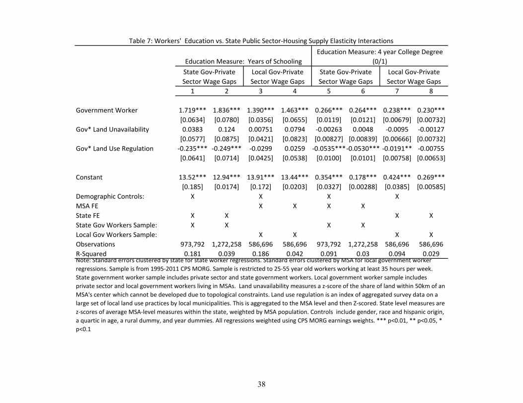
As an additional test of this alternative hypothesis, I assess whether public-private sector
workers years of education gaps vary with state and local housing supply elasticities. Table 7
preforms the standard analysis used to analyze state and local wage gaps, but replaces the left
hand side variable with a worker�s years of education. If government workers are higher skilled
that private sector workers in housing inelastic areas, then this should hold both for observed
skills (education) and unobserved skills (which cannot be tested). Table 7 shows that impact
of land unavailability on public-private sector education gaps is not statistically signi�cant.
This holds in the state government workers sample and local government workers sample.
This result is also robust to dropping worker demographics as controls in the regressions.
Overall, di¤erences in public and private sector workers�years of schooling to not appear to
relate to state and local housing supply elasticities. Columns 5 through 8 of Table 7 reports
additional robustness by re-doing the same analysis with the left-hand side variable equal
to a dummy of whether the worker has a four year college degree. These results further
show housing supply elasticity does not positively impact public-private sector worker skill
di¤erences. Government workers�wages appear to re�ect the market power of state and local
governments.
3.3 Bene�ts
Gittleman and Pierce (2012) show that government workers�bene�ts are more generous than
private sector workers�bene�ts. If the market power of state and local governments allows
22

government workers to earn more desirable wages than similar private sector workers, this
should also be true for public-private di¤erences in the generosity of bene�ts.
As a measure of government workers�pension bene�ts, I use data from the Census�2007-
2010 Annual Surveys of Public Employee Retirement Systems. This data is collected annually
from states governments�pension plans on the aggregate amount of retirement bene�ts paid
out during the year, as well as the total number of bene�ciaries who received a transfer that
year. Taking the ratio of these, gives the average pension payout per bene�ciary. Table 1
reports summary statistics on this data. Unfortunately, there is not a similar data set for
retirement payouts to private sector workers.
An indirect test of whether bene�ts augment or o¤set wage gap di¤erences is to assess
whether the state worker-private sector wage gap negatively varies with pension payouts per
retiree. If the public-private wage gap is high when public pension bene�ts are low, than
changes in wage gaps across states might be o¤set by changes in bene�ts across states. How-
ever, Table 9 shows a regression of state government pensions payouts per retiree is strongly
positively correlated with the public-private sector wage gap. This suggests that increases
in the public-private wage gap are positively associated with increases in the public-private
bene�ts gap. The wage gap estimates are likely a lower bound of impact of government mar-
ket power of government employees compensation since they do not account for the impacts
on bene�ts.
If private sector bene�ts do not vary with states� housing supply elasticities, than a
regression of state pension payouts per bene�ciary on states� housing supply elasticities
measures the impact of housing supply elasticity on government retirement bene�ts. Table
9 reports these regressions. I �nd a 1 standard deviation increases in a states�land unavail-
ability increases annual retirement payouts per retired state government employee by 0.0674
log points. Government workers appear to receive better compensation in both wages and
retirement bene�ts in areas where the government can exercise more market power.
23

4 Conclusion
By using housing supply elasticity as exogenous variation in governments�abilities to exercise
market power, I show that the public-private sector wage gap is higher in areas where the
government can extract more rent from residents. Further, this e¤ect is stronger for unionized
government workers, suggesting that public sector unions might in�uence governments to
engage in rent seeking behavior. While I cannot gauge to what extent government workers
are overcompensated overall, government market power appears to play a role in government
worker compensation.
The spatial equilibrium model shows that the scope of governments�market power does
not disappear when there is competition between a large number of governments or when
each government is small. The local labor and housing market will respond to the tax policy
choices of the state and local government, mitigating the disciplining e¤ects of workers�
voting with their feet through migration.
It is possible that the unmodeled political system where multiple candidates run for
election and campaign for less wasteful government policies could compete away some of this
government market power. However, the empirical evidence of this paper suggests that these
rents have not been fully competed away.
These results also speak to the welfare e¤ects of land-use regulation policy. While the
decision to regulate real-estate development and population expansion has many costs and
bene�ts not studied in this paper, my results show that decreasing a city�s housing supply
elasticity through regulation gives the local government more market power. Thus, the rise in
land-use regulations since the 1970s may have had an unintended consequence of increasing
rent seeking by governments and leading to overpaid government workers. State and local
governments appear to take advantage of their market power and some of these rents are
shared with government employees.
24

References
Autor, D.H. and Katz, L.F. and Kearney, M.S. (2008). Trends in us wage inequality:
Revising the revisionists. Review of Economics and Statistics.
Bollinger, C.R. and Hirsch, B.T. (2006). Match bias from earnings imputation in the
current population survey: The case of imperfect matching. Journal of Labor Eco-
nomics 24 (3), 483�519.
Brueckner, J.K. and Neumark, D. (2011). Beaches, sunshine, and public-sector pay: the-
ory and evidence on amenities and rent extraction by government workers. Technical
report, National Bureau of Economic Research.
Brueckner, Jan K. (1987). The structure of urban equilibria: A uni�ed treatment of the
muth-mills model. In E. S. Mills (Ed.), Handbook of Regional and Urban Economics,
Volume 2 of Handbook of Regional and Urban Economics, Chapter 20, pp. 821�845.
Elsevier.
Epple, D. and Zelenitz, A. (1981). The implications of competition among jurisdictions:
does tiebout need politics? The Journal of Political Economy, 1197�1217.
Freeman, R.B. (1986). Unionism comes to the public sector. Journal of Economic Litera-
ture, 41�86.
Gittleman, M. and Pierce, B. (2012). Compensation for state and local government work-
ers. The Journal of Economic Perspectives, 217�242.
Robert G. Gregory and Je¤ Borland. (1999). Chapter 53 recent developments in public
sector labor markets. Volume 3, Part C of Handbook of Labor Economics, pp. 3573 �
3630. Elsevier.
Gyourko, Joseph and Saiz, Albert and Summers, Anita. (2008). A new measure of the
local regulatory environment for housing markets: The wharton residential land use
regulatory index. Urban Studies 45 (3), 693�729.
25

Gyourko, J. and Tracy, J. (1991). The structure of local public �nance and the quality of
life. Journal of Political Economy, 774�806.
Krueger, A.B. (1988). Are public sector workers paid more than their alternative wage?
evidence from longitudinal data and job queues. InWhen public sector workers union-
ize, pp. 217�242. University of Chicago Press.
Roback, Jennifer. (1982). Wages, rents, and the quality of life. Journal of Political Econ-
omy 90 (6), pp. 1257�1278.
Rosen, Sherwin. (1979). Wages-based indexes of urban quality of life. In P. Mieszkowski
and M. Straszheim (Eds.), Current Issues in Urban Economics. John Hopkins Univ.
Press.
Saiz, Albert. (2010). The geographic determinants of housing supply. The Quarterly Jour-
nal of Economics 125 (3), pp. 1253�1296.
26

A Government Taxation under Income and PropertyTaxes
A.1 Income Tax
A.1.1 Government
The local government of city j charges an income tax � j to workers who choose to residewithin the city. The local government also produces government services, which cost sjfor each worker in the city. Nj measure the population of city j: The local rent seekinggovernment maximizes:
max�j ;sj
� jwjNj � sjNj
A.1.2 Workers
All workers are homogeneous. Workers living in city j inelastically supply one unit of labor,and earn wage wj: Each worker must rent a house to live in the city at rental rate rj and paythe local income tax � j:Workers value the local amenities as measure by Aj:The desirabilityof government services sj is represented by g (sj) : Thus, workers�utility from living in cityj is:
Uj = wj (1� � j)� rj + Aj + g (sj) :Workers maximize their utility by living in the city which they �nd the most desirable.
A.1.3 Firms
All �rms are homogenous and produce a tradeable output Y:Cities exogenously di¤er intheir productivity as measured by �j. Local government services impact �rms productivity,as measured by b(sj): The production function is:
Yj = �jNj + b(sj)Nj + F (Nj) ;
where F 0 (Nj) > 0 and F 00 (Nj) = 0 in labor: I assume a completely elastic labor demandcurve to focus on the role of housing supply elasticity in setting tax rates.The labor market is perfectly competitive, so wages equal the marginal product of labor:
wj = �j + b(sj) + F0 (Nj) :
A.1.4 Housing
The housing market is identical to the setting described in the main text in Section ##.The housing supply curve is:
rj = aj + j log (Nj) ;
j = xhousej
where xhousej is a vector of city characteristics which impact the elasticity of housing supply.
27

A.1.5 Equilibrium in Labor and Housing
Since all workers are identical, all cities with positive population must o¤er equal utility toworkers. In equilibrium, all workers must be indi¤erent between all cities. Thus:
Uj = wj (1� � j)� rj + Aj + g (sj) = �U:
Plugging in labor demand and housing supply gives:
(�j + b(sj) + F0 (Nj)) (1� � j)� aj � j logNj + Aj + g (sj) = �U: (7)
Equation (7) determines the equilibrium distribution of workers across cities.
A.1.6 Government Tax Competition
The government maximizes:maxsj ;�j
� jwjNj � sjNj:
The �rst order conditions are:
0 = wj� j@Nj@sj
+ � jNj@wj@Nj
@Nj@sj
�Nj � sj@Nj@sj
(8)
0 = � j
�@wj@Nj
@Nj@� j
Nj + wj@Nj@� j
�+ wjNj � sj
@Nj@� j
:
Di¤erentiating equation (7) to solve for @Nj@sj
and @Nj@�jgives:
@Nj@sj
= Nj(1� � j) b0 (sj) + g0 (sj)
j> 0
@Nj@� j
= �Nj(�j + b(sj) + F
0 (Nj))
j< 0: (9)
Population increases with government services and decreases in taxes. Plugging these into(8) and combining the �rst order conditions shows that government services are providedsuch that the marginal bene�t
��1� � �j
�b0 (sj) + g
0 (sj)�equals marginal cost (1) :�
1� � �j�b0�s�j�+ g0
�s�j�= 1:
This is the socially optimal level of government service, given the tax rate.The equilibrium tax revenue per capita is:
wj��j = j + s
�j : (10)
To analyze the e¤ect of housing supply elasticity on governments�ability to extract rentfrom taxes, I di¤erentiate the tax markup with respect to the slope of the inverse housing
28

supply curve, j:@
@ j
�wj�
�j � s�j
�= 1 > 0: (11)
The government can extract more rent through higher taxes in a city with a less elastichousing supply with a income tax instrument.
A.2 Property Tax
A.2.1 Government
The local government of city j charges a property tax � j to workers who choose to residewithin the city. The local rent seeking government maximizes:
max�j ;sj
� jrjNj � sjNj
A.2.2 Workers
Workers�utility from living in city j facing a property tax � j is:
Uj = wj � rj (1 + � j) + Aj + g (sj) :
A.2.3 Firms
The production function is:
Yj = �jNj + b(sj)Nj + F (Nj) ;
where F 0 (Nj) > 0 and F 00 (Nj) = 0 in labor: I assume a completely elastic labor demandcurve to focus on the role of housing supply elasticity in setting tax rates.The labor market is perfectly competitive, so wages equal the marginal product of labor:
wj = �j + b(sj) + F0 (Nj) :
A.2.4 Housing
The housing market is identical to the setting described in the main text in Section ##.The housing supply curve is:
rj = aj + j log (Nj) ;
j = xhousej
where xhousej is a vector of city characteristics which impact the elasticity of housing supply.
29

A.2.5 Equilibrium in Labor and Housing
Since all workers are identical, all cities with positive population must o¤er equal utility toworkers. In equilibrium, all workers must be indi¤erent between all cities. Thus:
Uj = wj � rj (1 + � j) + Aj + g (sj) = �U:
Plugging in labor demand and housing supply gives:
(�j + b(sj) + F0 (Nj))�
�aj + j logNj
�(1 + � j) + Aj + g (sj) = �U: (12a)
Equation (7) determines the equilibrium distribution of workers across cities.
A.2.6 Government Tax Competition
The government maximizes:maxsj ;�j
� jrjNj � sjNj:
The �rst order conditions are:
0 = rj� j@Nj@sj
+ � jNj@rj@Nj
@Nj@sj
�Nj � sj@Nj@sj
(13)
0 = � j
�@rj@Nj
@Nj@� j
Nj + rj@Nj@� j
�+ rjNj � sj
@Nj@� j
: (14)
Di¤erentiating equation (7) to solve for @Nj@sj
and @Nj@�jgives:
@Nj@sj
= Njb0 (sj) + g
0 (sj)
j (1 + � j)> 0
@Nj@� j
= �Njrj
j (1 + � j)< 0: (15)
Combining the �rst order conditions shows that government services are provided such thatthe marginal bene�t (b0 (sj) + g0 (sj)) equals marginal cost (1) ; which is the same �nding foran income tax and head tax:
b0�s�j�+ g0
�s�j�= 1:
Plugging (15) into (14) and rearranging shows the equilibrium tax revenue per capita is:
rj��j = j + s
�j : (16)
Di¤erentiating the tax markup with respect to the slope of the inverse housing supply curve, j:
@
@ j
�wj�
�j � s�j
�= 1 > 0: (17)
The government can extract more rent through higher taxes in a city with a less elastic
30

housing supply using a property tax instrument. In the case of a property tax, as opposed toa head tax, there are four mechanisms through which a tax rate change impacts governmentrevenue. To break these down, I rewrite the tax rate �rst order condition:
0 = � jrj@Nj@� j| {z }
Decline in revenue due
to population decrease
+ � j@rj@Nj
@Nj@� j
Nj| {z }Decline in revenue
due to rent decrease
+ rjNj|{z}Additional tax revenue
from each resident
� sj@Nj@� j| {z }
Government services
cost savings
(18)First, the amount of out-migration driven by a tax hike is in�uenced by the local housing
supply elasticity. This is the �rst term of equation (18) : Second, the out-migration lowersrents and directly impacts tax revenues since the tax revenue is a percentage of housing rents.This is the second term of equation (18) : However, the housing supply elasticity will notimpact the size of the rental rate decrease in response to a tax hike. To see this, recall theequilibrium condition, equation (12a) : For workers to derive utility �U from this local area,the utility impact of a tax increase must be perfectly o¤set by a rent decrease.6 Thus, theequilibrium rental rate response to a given tax increase does not depend on the local housingsupply elasticity. Indeed, the housing supply elasticity determines the migration responserequired to change housing rents in order to o¤set the utility impact of the tax increase.Thus, a more inelastic housing supply decreases the elasticity of government revenue withrespect to the tax rate, giving the government more market power when using a propertytax instrument.The third and forth terms of equation (18) show a tax increase raises government revenues
from each household and lowers the cost of government services due to out-migration. Thesechannels also appear in the case of a head tax instrument.
6Since I have assumed a perfectly elastic labor demand curve, the rental rate response to a tax increasewould be the same in any city. However, if labor demand was not perfectly elastic, then the rental rateresponse to a tax increase could di¤er with housing supply elasticity, since housing supply elasticity wouldin�uence the relative incidence of the tax rate on wages versus rents.
31

Mean
Standard
Dev. Min Max N
Local Government Worker Ln Weekly
Earnings 6.723 0.519 4.854 8.695 112639
State Government Worker Ln Weekly
Earnings 6.725 0.509 4.857 8.695 62994
Federal Government Worker Ln
Weekly Earnings 6.964 0.496 4.855 8.695 37008
Private Sector Worker Ln Weekly
Earnings 6.686 0.613 4.852 8.695 968349
Mean
Standard
Dev. Min Max N
State Aggregated Land Unavailability: Z-
Score 0.000 1.000 -1.427 2.982 48
State Aggregated Wharton Land Use
Regulation Index: Z-Score 0.000 1.000 -1.640 2.348 48
MSA Land Unavailability: Z-Score 0.000 1.000 -1.205 2.824 228
MSA Wharton Land Use Regulation
Index: Z-Score 0.000 1.000 -1.746 3.938 228
Mean
Standard
Dev. Min Max N
Log Thousand Dollars of Annual Payout
per beneficiary from State Pension 2.9897 0.24996 2.5289 3.629 192
Table 1: Summary Statistics
A. CPS Data 1995-2011
B. Housing Supply Elasticity Measures
C. State Government Pension Payouts: 2007-2010
Notes: Wages are measured as weekly wages deflated by the CPI-U and reported in constant 2011 dollars
for 25-55 year old workers working at least 35 hours per week. Workers with imputed weekly earnings
are dropped from the analysis. Top coded weekly earnings as set to 1.5 times the top coded value and
weekly earnings below $128 (in real 2011 dollars) are dropped from the analysis. Sector of worker
(local/state/federal/private) is measured by reported class of worker. MSA land unavailability measures
the share of land within 50km of an MSA's center which cannot be developed due to these topological
constraints from Saiz (2010). This measure is then Z-scored. The Wharton Land Use Regulation index
aggregates survey data on a large set of local land use practices by local municipalities. This is aggregated
to the MSA level and then Z-scored. State aggregated housing supply elasticity meaures use a population
weighted average of MSA level data. State and MSA level housing supply elasticity measures are z-scored.
Government pension data come from 2007-2010 Annual Surveys of Public-Employee Retirement
Systems.
32

1 2 3 4 5 6
Government Worker -0.112*** -0.113*** -0.0798***-0.0707***
[0.00909] [0.00931] [0.00721] [0.00758]
Gov* Land Unavailability 0.0170* 0.0262*** 0.0287*** 0.0366*** 0.00856 0.0108*
[0.0101] [0.00976] [0.00781] [0.00855] [0.00637] [0.00657]
Gov* Land Use Regulation 0.0263** 0.0348*** 0.0220**
[0.0125] [0.00803] [0.00920]
Constant 2.493*** 2.487*** 2.382*** 2.378*** 2.396*** 2.399***
[0.289] [0.290] [0.397] [0.396] [0.397] [0.397]
State x Gov Worker FE: X X
State Elasticity Measures: X X
MSA Elasticity Measures: X X X X
State Gov Workers Sample: X X
Local Gov Workers Sample: X X X X
Observations 973,792 973,792 586,696 586,696 586,696 586,696
R-squared 0.384 0.384 0.389 0.389 0.39 0.39
Table 2: Ln Wage vs. State & Local Public Sector-Housing Supply Elasticity Interactions
Note: Standard errors clustered by state for state worker regressions. Standard errors clustered by MSA for local
government worker regressions. Weekly wage data from 1995-2011 CPS MORG. Wage data is restricted to 25-55
year old workers working at least 35 hours per week. State government worker sample includes private sector
and state government workers. Local government worker sample includes private sector and local government
workers living in MSAs. Land unavailability measures a z-score of the share of land within 50km of an MSA's
center which cannot be developed due to topological constraints. Land use regulation is an index of aggregated
survey data on a large set of local land use practices by local municipalities. This is aggregated to the MSA level
and then Z-scored. State level measures are z-scores of average MSA-level measures within the state, weighted
by MSA population. Controls include 15 dummies for education categories, gender, race and hispanic origin, a
quartic in age, a rural dummy, and year dummies. All regressions weighted using CPS MORG earnings weights.
State Gov-Private
Sector Wage Gaps Local Gov-Private Sector Wage Gaps
33

1 2 3 4
Government Worker -0.0320***-0.0331*** 0.0181*** 0.0275***
[0.00830] [0.00837] [0.00538] [0.00545]
Gov* Land Unavailability 0.0107 0.0188* 0.0197*** 0.0275***
[0.0111] [0.0109] [0.00675] [0.00743]
Gov* Land Use Regulation 0.0234** 0.0350***
[0.0112] [0.00716]
Constant 4.263*** 4.258*** 4.211*** 4.208***
[0.274] [0.274] [0.386] [0.386]
State Elasticity Measures: X X
MSA Elasticity Measures: X X
State Gov Workers Sample: X X
Local Gov Workers Sample: X X
Observations 973,792 973,792 586,696 586,696
R-squared 0.524 0.524 0.526 0.526
Table 3: Ln Wage vs. State & Local Public Sector-Housing Supply Elasticity
Interactions with 3 Digit Occupation Dummy controls
Note: Standard errors clustered by state for state worker regressions. Standard errors
clustered by MSA for local government worker regressions. Weekly wage data from
1995-2011 CPS MORG. Wage data is restricted to 25-55 year old workers working at
least 35 hours per week. State government worker sample includes private sector and
state government workers. Local government work sampe includes private sector and
local government workers living in MSAs. Land unavailability measures a z-score of the
share of land within 50km of an MSA's center which cannot be developed due to
topological constraints. Land use regulation is an index of aggregated survey data on a
large set of local land use practices by local municipalities. This is aggregated to the
MSA level and then Z-scored. State level measures are z-scores of average MSA-level
measures within the state, weighted by MSA population. Controls include 1057
occupation dummies, 15 dummies for education categories, gender, race, hispanic
origin, a quartic in age, a rural dummy, and year dummies. Three digit occupation code
definitions change in 2000, so I include the full set of combined 3 digit occupation
dummies. I treat occupation codes used in years 2000-2011 as distinct occupations
from those in previous years, giving a total of 1057 occupation codes. All regressions
weighted using CPS earnings weights. *** p<0.01, ** p<0.05, * p<0.1
State Gov-Private
Sector Wage Gaps
Local Gov-Private
Sector Wage Gaps
34

1 2 3 4
Government Worker -0.140*** -0.142*** -0.123*** -0.119***
[0.00613] [0.00575] [0.00695] [0.00718]
Gov* Land Unavailability 0.0101 0.0127** 0.0269*** 0.0316***
[0.00705] [0.00624] [0.00739] [0.00801]
Gov* Land Use Regulation 0.00782 0.0238***
[0.00889] [0.00801]
Gov* Land Unavailability*Union 0.00372 0.0214* -0.00373 0.00753
[0.0120] [0.0128] [0.00845] [0.00934]
Gov* Land Use Regulation*Union 0.0492** 0.0356***
[0.0191] [0.0106]
Constant 2.532*** 2.540*** 2.456*** 2.442***
[0.289] [0.288] [0.395] [0.396]
State Elasticity Measures: X X
MSA Elasticity Measures: X X
State Gov Workers Sample: X X
Local Gov Workers Sample: X X
973,792 973,792 586,696 586,696
0.39 0.389 0.395 0.394
Table 4: Ln Wage vs. State & Local Public Sector-Housing Supply Elasticity
Interactions: Union Government Workers
Note:Standard errors clustered by state for state worker regressions. Standard errors
clustered by MSA for local government worker regressions. Weekly wage data from 1995-
2011 CPS MORG. Wage data is restricted to 25-55 year old workers working at least 35 hours
per week. State government worker sample includes private sector and state government
workers. Local government work sampe includes private sector and local government
workers living in MSAs. Land unavailability measures a z-score of the share of land within
50km of an MSA's center which cannot be developed due to topological constraints. Land
use regulation is an index of aggregated survey data on a large set of local land use practices
by local municipalities. This is aggregated to the MSA level and then Z-scored. State level
measures are z-scores of average MSA-level measures within the state, weighted by MSA
population. Controls include 15 dummies for education categories, gender, race and
hispanic origin, a quartic in age, a rural dummy, and year dummies. Controls also include a
labor union dummy, labor union dummy interacted with government dummy, and the labor
union dummy interacted with the housing supply elasticity measures. Union is defined as a
member of a labor union. All regressions weighted using CPS earnings weights. *** p<0.01,
** p<0.05, * p<0.1
State Gov-Private
Sector Wage Gaps
Local Gov-Private
Sector Wage Gaps
35

1 2 3 4 5 6 7 8
Government Worker -0.182*** -0.182*** -0.123*** -0.119*** -0.0183 -0.0201 -0.0361*** -0.0221**
[0.00837] [0.00832] [0.00852] [0.00866] [0.0130] [0.0143] [0.00845] [0.00949]
Gov* Land Unavailability 0.0113* 0.00889* 0.0231*** 0.0271*** 0.0243* 0.0424*** 0.0359*** 0.0481***
[0.00644] [0.00518] [0.00880] [0.00894] [0.0142] [0.0148] [0.00881] [0.0102]
Gov* Land Use Regulation -0.00686 0.0169* 0.0520*** 0.0563***
[0.00981] [0.00994] [0.0156] [0.00959]
Constant 2.767*** 2.773*** 2.788*** 2.791*** 2.472*** 2.471*** 2.393*** 2.379***
[0.768] [0.769] [0.840] [0.840] [0.325] [0.325] [0.434] [0.434]
State Elasticity Measures: X X X X
MSA Elasticity Measures: X X X X
State Gov Workers Sample: X X X X
Local Gov Workers Sample: X X X X
Observations 307,951 307,951 201,691 201,691 665,841 665,841 385,005 385,005
R-squared 0.227 0.227 0.229 0.229 0.26 0.26 0.278 0.277
College Sample Non-College Sample
Table 5: Ln Wage vs. State & Local Public Sector-Housing Supply Elasticity Interactions: Subsamples by College Education of
Workers
Note: Standard errors clustered by state for state worker regressions. Standard errors clustered by MSA for local government worker
regressions. Weekly wage data from 1995-2011 CPS MORG. Wage data is restricted to 25-55 year old workers working at least 35 hours
per week. State government worker sample includes private sector and state government workers. Local government worker sample
includes private sector and local government workers living in MSAs. Land unavailability measures a z-score of the share of land within
50km of an MSA's center which cannot be developed due to topological constraints. Land use regulation is an index of aggregated survey
data on a large set of local land use practices by local municipalities. This is aggregated to the MSA level and then Z-scored. State level
measures are z-scores of average MSA-level measures within the state, weighted by MSA population. Controls include 15 dummies for
education categories, gender, race and hispanic origin, a quartic in age, a rural dummy, and year dummies. All regressions weighted using
CPS MORG earnings weights. *** p<0.01, ** p<0.05, * p<0.1
State Gov-Private
Sector Wage Gaps
Local Gov-Private
Sector Wage Gaps
State Gov-Private
Sector Wage Gaps
Local Gov-Private
Sector Wage Gaps
36

1 2 3 4 5 6
Government Worker 0.162*** 0.161*** 0.158*** 0.154***
[0.0130] [0.0130] [0.00701] [0.00748]
Gov* Land Unavailability -0.0172 -0.0216** -0.00698 -0.00972 -0.0122 -0.0117
[0.0112] [0.0103] [0.00805] [0.00776] [0.00786] [0.00793]
Gov* Land Use Regulation -0.0151 -0.0158 0.00625
[0.0122] [0.0114] [0.0100]
Constant 2.338*** 2.337*** 2.422*** 2.418*** 2.701*** 2.701***
[0.291] [0.291] [0.413] [0.412] [0.413] [0.413]
State FE X X
MSA FE X X X X
State x Gov Worker FE: X X
State Elasticity Measures: X X
MSA Elasticity Measures: X X X X
Federal Gov Worker Sample: X X X X
State Gov Workers Sample: X X
Note: Standard errors clustered by 948,785 948,785 549,857 549,857 560,367 560,367
0.383 0.383 0.394 0.394 0.39 0.39
Table 6: State & Federal Government Workers Falsification Tests
Note:Standard errors clustered by state for state worker regressions. Standard errors clustered by MSA for local
government worker regressions. Weekly wage data from 1995-2011 CPS MORG. Wage data is restricted to 25-55
year old workers working at least 35 hours per week. State government worker sample includes private sector
and state government workers. Federal government work sampe includes private sector and federal government
workers. Land unavailability measures a z-score of the share of land within 50km of an MSA's center which
cannot be developed due to topological constraints. Land use regulation is an index of aggregated survey data
on a large set of local land use practices by local municipalities. This is aggregated to the MSA level and then Z-
scored. State level measures are z-scores of average MSA-level measures within the state, weighted by MSA
population. Controls include 15 dummies for education categories, gender, race, hispanic origin, a quartic in
age, a rural dummy, and year dummies. All regressions weighted using CPS earnings weights. *** p<0.01, **
p<0.05, * p<0.1
State Gov-Private
Sector Wage GapsFederal Gov-Private Sector Wage Gaps
37
1 2 3 4 5 6 7 8
Government Worker 1.719*** 1.836*** 1.390*** 1.463*** 0.266*** 0.264*** 0.238*** 0.230***
[0.0634] [0.0780] [0.0356] [0.0655] [0.0119] [0.0121] [0.00679] [0.00732]
Gov* Land Unavailability 0.0383 0.124 0.00751 0.0794 -0.00263 0.0048 -0.0095 -0.00127
[0.0577] [0.0875] [0.0421] [0.0823] [0.00827] [0.00839] [0.00666] [0.00732]
Gov* Land Use Regulation -0.235*** -0.249*** -0.0299 0.0259 -0.0535***-0.0530*** -0.0191** -0.00755
[0.0641] [0.0714] [0.0425] [0.0538] [0.0100] [0.0101] [0.00758] [0.00653]
Constant 13.52*** 12.94*** 13.91*** 13.44*** 0.354*** 0.178*** 0.424*** 0.269***
[0.185] [0.0174] [0.172] [0.0203] [0.0327] [0.00288] [0.0385] [0.00585]
Demographic Controls: X X X X
MSA FE X X X X
State FE X X X X
State Gov Workers Sample: X X X X
Local Gov Workers Sample: X X X X
Observations 973,792 1,272,258 586,696 586,696 973,792 1,272,258 586,696 586,696
R-Squared 0.181 0.039 0.186 0.042 0.091 0.03 0.094 0.029
Local Gov-Private
Sector Wage Gaps
Table 7: Workers' Education vs. State Public Sector-Housing Supply Elasticity Interactions
Education Measure: Years of Schooling
Education Measure: 4 year College Degree
(0/1)
Note: Standard errors clustered by state for state worker regressions. Standard errors clustered by MSA for local government worker
regressions. Sample is from 1995-2011 CPS MORG. Sample is restricted to 25-55 year old workers working at least 35 hours per week.
State government worker sample includes private sector and state government workers. Local government worker sample includes
private sector and local government workers living in MSAs. Land unavailability measures a z-score of the share of land within 50km of an
MSA's center which cannot be developed due to topological constraints. Land use regulation is an index of aggregated survey data on a
large set of local land use practices by local municipalities. This is aggregated to the MSA level and then Z-scored. State level measures are
z-scores of average MSA-level measures within the state, weighted by MSA population. Controls include gender, race and hispanic origin,
a quartic in age, a rural dummy, and year dummies. All regressions weighted using CPS MORG earnings weights. *** p<0.01, ** p<0.05, *
p<0.1
State Gov-Private
Sector Wage Gaps
Local Gov-Private
Sector Wage Gaps
State Gov-Private
Sector Wage Gaps
38
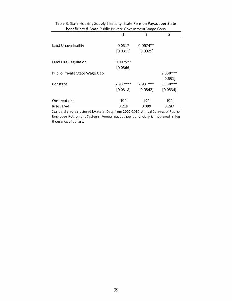
1 2 3
Land Unavailability 0.0317 0.0674**
[0.0311] [0.0329]
Land Use Regulation 0.0925**
[0.0366]
Public-Private State Wage Gap 2.830***
[0.651]
Constant 2.932*** 2.931*** 3.130***
[0.0318] [0.0342] [0.0534]
Observations 192 192 192
R-squared 0.219 0.099 0.287
Standard errors clustered by state. Data from 2007-2010 Annual Surveys of Public-
Employee Retirement Systems. Annual payout per beneficiary is measured in log
thousands of dollars.
Table 8: State Housing Supply Elasticity, State Pension Payout per State
beneficiary & State Public-Private Government Wage Gaps
39

Figure 1: State Goverment-Private Sector Wages Gaps vs. State Land Unavailability Z-Score
AL
AZ
AR
CA
CO
CT
DEFL
GA
ID
IL
IN
IA
KS
KY LA
ME
MDMA
MI
MN
MS
MO
MT
NE
NV
NH
NJ
NM
NY
NCND
OH
OK
OR
PA RI
SC
SD
TN
TX
UT
VT
VA
WA
WV
WI
WY
.2.1
5.1
.05
0Pu
blic
Priv
ate
Wag
e G
ap
1 0 1 2 3State Average Land Unavai labil i ty in MSAs: ZScore
Notes: State wage gaps calculated after residualizing wages against 15 dummies foreducation categories, gender, race, hispanic origin, a quartic in age, a rural dummy, and
year dummies. Regression weighted using CPS earnings weights.
40

Figure 2: Local Goverment-Private Sector Wages Gaps vs. MSA Land Unavailability Z-Score
Atlanta
Baltimore
Boston
ChicagoClevelandDetroit
HoustonKansasCity
LasVegas
LA
Minneapolis
NYC
PhiladelphiaPhoeniz
Pittsburgh
PortlandStLouis
SaltLake
Washington
.6.4
.20
.2Pu
blic
Priv
ate
Wag
e G
ap
1 0 1 2 3MSA Land Unavai labil i ty: ZScore
Notes: MSA wage gaps calculated after residualizing wages against 15 dummies foreducation categories, gender, race, Hispanic origin, a quartic in age, a rural dummy, and
year dummies. Regression weighted using CPS earnings weights.
41