Embed Size (px)
Citation preview
Technical Report No. 106 / Rapport technique no 106
Household Risk Assessment Model
by Brian Peterson and Tom Roberts
The views expressed in this report are solely those of the authors. No responsibility for them should be attributed to the Bank of Canada.
ISSN 1919-689X © 2016 Bank of Canada
September 2016
Household Risk Assessment Model
Brian Peterson and Tom Roberts
Financial Stability Department Bank of Canada
Ottawa, Ontario, Canada K1A 0G9 [email protected] [email protected]

ii
Acknowledgements
We would like to thank Ian Christensen, Allan Crawford, Bradley Howell, Césaire Meh, Miguel Molico and Virginie Traclet for useful comments and suggestions. A special acknowledgment goes to Ramdane Djoudad, Umar Faruqui and Xuezhi Liu for their roles in previous versions of the model.
iii
Abstract
Household debt can be an important source of vulnerability to the financial system. This technical report describes the Household Risk Assessment Model (HRAM) that has been developed at the Bank of Canada to stress test household balance sheets at the individual level. In addition to stress testing, HRAM is flexible enough to analyze the effects of a variety of shocks (such as an increase in mortgage rates) and changes to policy, including both monetary policy and macroprudential regulation. The model’s strength is its ability to exploit information from survey microdata on the distribution of debt, assets and income across Canadian households. JEL classification: C0, C6, C63, C65, D0, D1, D14 Bank classification: Financial stability; Housing; Sectoral balance sheet
Résumé
La dette des ménages peut constituer une importante source de vulnérabilité pour le système financier. Le présent rapport technique se propose de décrire le modèle d’évaluation des risques dans le secteur des ménages (modèle HRAM) conçu par la Banque du Canada pour tester, au niveau microéconomique, la capacité de résistance des bilans des ménages. Le modèle HRAM offre en outre la souplesse nécessaire pour permettre l’analyse des effets de chocs divers (tels qu’une hausse des taux hypothécaires) et de l’évolution des politiques publiques, tant la politique monétaire que la réglementation macroprudentielle. Le modèle se distingue par sa capacité à exploiter le contenu informatif de microdonnées d’enquête utilisées pour établir la distribution des dettes, des actifs et des revenus des ménages canadiens.
Classification JEL : C0, C6, C63, C65, D0, D1, D14 Classification de la Banque : Stabilité financière; Logement; Bilan sectoriel
Contents
1 Introduction 5
2 Overview of HRAM Approach 6
2.1 Key Modelling Features . . . . . . . . . . . . . . . . . . . . . . . . . 6
2.2 Steps in an HRAM Simulation . . . . . . . . . . . . . . . . . . . . . . 9
3 General Methodology: Macro-Consistent Micro-Simulation 11
3.1 Households . . . . . . . . . . . . . . . . . . . . . . . . . . . . . . . . 12
3.2 Evolution of Household Variables: Macro-Consistent Micro-Simulation 13
3.2.1 Macro scenario . . . . . . . . . . . . . . . . . . . . . . . . . . 14
3.2.2 Idiosyncratic shocks . . . . . . . . . . . . . . . . . . . . . . . . 15
3.2.3 Intermediate household variables: Law of motion . . . . . . . 16
3.2.4 Consistency factors: Macro restrictions . . . . . . . . . . . . . 16
3.2.5 Final household variables: Allocation function . . . . . . . . . 17
3.2.6 Definition of a macro-consistent micro-simulation . . . . . . . 17
4 The Model 17
4.1 Evolution of Income and Employment . . . . . . . . . . . . . . . . . . 18
4.1.1 Unemployment and unemployment duration . . . . . . . . . . 18
4.1.2 Permanent labour income . . . . . . . . . . . . . . . . . . . . 21
4.2 Evolution of Household Balance Sheet . . . . . . . . . . . . . . . . . 22
4.2.1 Debt payments . . . . . . . . . . . . . . . . . . . . . . . . . . 23
4.2.2 Housing purchases: First-time homebuyers . . . . . . . . . . . 25
4.2.3 Mortgage debt: Non-first-time homebuyers . . . . . . . . . . . 27
4.2.4 Consumer debt . . . . . . . . . . . . . . . . . . . . . . . . . . 28
4.2.5 Evolution of housing assets . . . . . . . . . . . . . . . . . . . . 30
4.2.6 Savings: Accumulation of financial assets . . . . . . . . . . . . 30
4.2.7 Lines of credit . . . . . . . . . . . . . . . . . . . . . . . . . . . 31
4.2.8 Arrears . . . . . . . . . . . . . . . . . . . . . . . . . . . . . . 31
5 Data 32
5.1 Missing Values . . . . . . . . . . . . . . . . . . . . . . . . . . . . . . 35
6 Estimation and Calibration 39
6.1 Income and Debt Equations . . . . . . . . . . . . . . . . . . . . . . . 41
6.2 Unemployment . . . . . . . . . . . . . . . . . . . . . . . . . . . . . . 41
6.3 Unemployment Duration . . . . . . . . . . . . . . . . . . . . . . . . . 43
2
6.4 Employment Insurance . . . . . . . . . . . . . . . . . . . . . . . . . . 44
6.5 Mortgage Parameters for a First-Time Homebuyer . . . . . . . . . . . 45
6.6 Arrears Process . . . . . . . . . . . . . . . . . . . . . . . . . . . . . . 45
6.7 Credit Growth Allocation to First-Time Homebuyers . . . . . . . . . 46
6.8 Taxes . . . . . . . . . . . . . . . . . . . . . . . . . . . . . . . . . . . . 46
7 Illustrative Scenarios and Comparative Statics 47
7.1 Back-Testing Exercise . . . . . . . . . . . . . . . . . . . . . . . . . . 47
7.2 Other Illustrative Scenarios . . . . . . . . . . . . . . . . . . . . . . . 48
7.3 Describing Households in Arrears . . . . . . . . . . . . . . . . . . . . 52
8 Conclusions 56
References 57
Appendix A List of Variables 59
A.1 Household Fixed Characteristics (Ωi) . . . . . . . . . . . . . . . . . . 59
A.2 Household Variables (Xi,t) . . . . . . . . . . . . . . . . . . . . . . . . 60
A.3 Household Idiosyncratic Shocks (εi,t) . . . . . . . . . . . . . . . . . . 62
A.4 Macro Scenario (Zt) . . . . . . . . . . . . . . . . . . . . . . . . . . . 63
A.5 Consistency Factors (Ct) . . . . . . . . . . . . . . . . . . . . . . . . . 63
A.6 Other Parameters . . . . . . . . . . . . . . . . . . . . . . . . . . . . . 64
Appendix B Back-Test Scenario 65
List of Tables
1 Balance Sheet for Household i in Period t . . . . . . . . . . . . . . . . 23
2 Percentage of Indebted Households, by Income Quartile . . . . . . . . 35
3 Percentage of Indebted Households, by Age Group . . . . . . . . . . . 36
4 Parameters . . . . . . . . . . . . . . . . . . . . . . . . . . . . . . . . 39
4 Parameters . . . . . . . . . . . . . . . . . . . . . . . . . . . . . . . . 40
4 Parameters . . . . . . . . . . . . . . . . . . . . . . . . . . . . . . . . 41
5 Assumptions for an Illustrative Stress-Test Scenario . . . . . . . . . . 49
6 Percentage Increase in Arrears as a Result of Changes in Unemploy-
ment and Interest Rates . . . . . . . . . . . . . . . . . . . . . . . . . 52
7 Percentage Increase in Arrears as a Result of Changes in Asset Avail-
ability . . . . . . . . . . . . . . . . . . . . . . . . . . . . . . . . . . . 52
8 Mean Characteristics of Indebted Households, by Arrears Status . . . 53
3
9 Mean Characteristics of Indebted Households, by Region . . . . . . . 55
B.1 Back-Test Scenario, 2006-2011 . . . . . . . . . . . . . . . . . . . . . . 65
List of Figures
1 Flow Chart of HRAM Structure . . . . . . . . . . . . . . . . . . . . . 10
2 Household Financial Characteristics . . . . . . . . . . . . . . . . . . . 33
3 Debt-Service Ratio Distribution, 2013 . . . . . . . . . . . . . . . . . . 36
4 Debt-Service Ratio Distribution, 2013 . . . . . . . . . . . . . . . . . . 37
5 Asset-Coverage Distribution, 2013 . . . . . . . . . . . . . . . . . . . . 37
6 Complete vs. Incomplete Duration . . . . . . . . . . . . . . . . . . . 44
7 Reported Incomplete Duration . . . . . . . . . . . . . . . . . . . . . . 45
8 Stock vs. Flow of Arrears . . . . . . . . . . . . . . . . . . . . . . . . 46
9 Back-Testing Results . . . . . . . . . . . . . . . . . . . . . . . . . . . 48
10 Results for an Illustrative Stress-Test Scenario . . . . . . . . . . . . . 51
11 Household Arrears Rate, by Starting-Point Vulnerabilities . . . . . . 54
12 Distributions for Starting-Point Vulnerabilities . . . . . . . . . . . . . 54
4
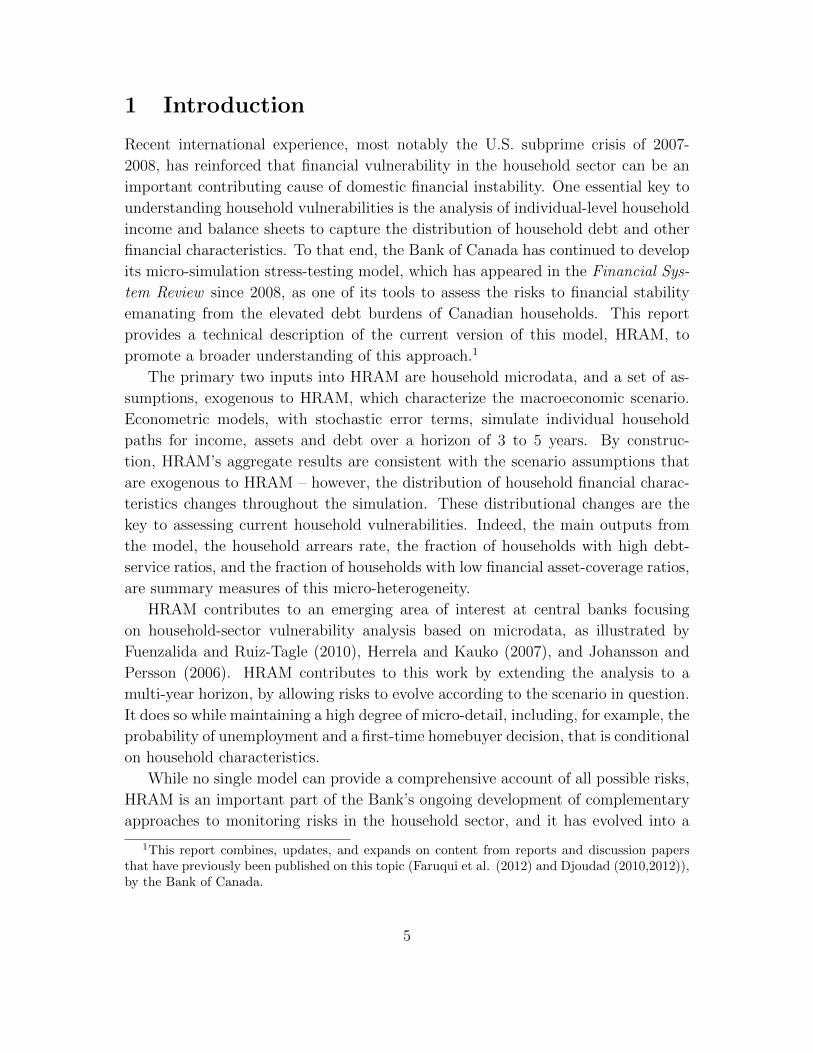
1 Introduction
Recent international experience, most notably the U.S. subprime crisis of 2007-
2008, has reinforced that financial vulnerability in the household sector can be an
important contributing cause of domestic financial instability. One essential key to
understanding household vulnerabilities is the analysis of individual-level household
income and balance sheets to capture the distribution of household debt and other
financial characteristics. To that end, the Bank of Canada has continued to develop
its micro-simulation stress-testing model, which has appeared in the Financial Sys-
tem Review since 2008, as one of its tools to assess the risks to financial stability
emanating from the elevated debt burdens of Canadian households. This report
provides a technical description of the current version of this model, HRAM, to
promote a broader understanding of this approach.1
The primary two inputs into HRAM are household microdata, and a set of as-
sumptions, exogenous to HRAM, which characterize the macroeconomic scenario.
Econometric models, with stochastic error terms, simulate individual household
paths for income, assets and debt over a horizon of 3 to 5 years. By construc-
tion, HRAM’s aggregate results are consistent with the scenario assumptions that
are exogenous to HRAM – however, the distribution of household financial charac-
teristics changes throughout the simulation. These distributional changes are the
key to assessing current household vulnerabilities. Indeed, the main outputs from
the model, the household arrears rate, the fraction of households with high debt-
service ratios, and the fraction of households with low financial asset-coverage ratios,
are summary measures of this micro-heterogeneity.
HRAM contributes to an emerging area of interest at central banks focusing
on household-sector vulnerability analysis based on microdata, as illustrated by
Fuenzalida and Ruiz-Tagle (2010), Herrela and Kauko (2007), and Johansson and
Persson (2006). HRAM contributes to this work by extending the analysis to a
multi-year horizon, by allowing risks to evolve according to the scenario in question.
It does so while maintaining a high degree of micro-detail, including, for example, the
probability of unemployment and a first-time homebuyer decision, that is conditional
on household characteristics.
While no single model can provide a comprehensive account of all possible risks,
HRAM is an important part of the Bank’s ongoing development of complementary
approaches to monitoring risks in the household sector, and it has evolved into a
1This report combines, updates, and expands on content from reports and discussion papersthat have previously been published on this topic (Faruqui et al. (2012) and Djoudad (2010,2012)),by the Bank of Canada.
5
flexible tool that can consider a wide array of alternative scenarios.
This report is organized as follows. Section 2 provides an overview of the ap-
proach used, covering key modelling features and the steps involved in an HRAM
simulation. Section 3 describes the conceptual model structure, emphasizing the role
of the exogenous scenario assumptions as inputs for the model. Section 4 provides
the details of the specific equations that make up HRAM. The data used to initial-
ize the model are covered in Section 5, while Section 6 discusses calibration. Some
examples of simulation results are illustrated in Section 7. Section 8 concludes.
2 Overview of HRAM Approach
The goal of HRAM is to simulate the impacts of large macroeconomic shocks at the
micro household level, where non-linearities, financial frictions, and heterogeneity
play a large role. All three features are essential to stress testing the household
sector since we are trying to capture default on debt, by a subset of households,
which is inherently a non-linear financial outcome. The inputs into the model are a
scenario for the macroeconomic environment, called a “macro scenario”, and data
at the household level that incorporate a significant amount of household-level het-
erogeneity. The outputs are aggregate statistics of observations at the micro level,
such as the arrears rate on household debt and the percentage of households that
have a “vulnerable” balance sheet owing to high debt-to-income ratios or large debt-
servicing burdens relative to income.
By construction, HRAM is meant to complement other policy models, especially
rational forward-looking dynamic stochastic general-equilibrium (DSGE) models.
Such DSGE models, while elegant and with good predictive powers, also come with
strong restrictions that limit their ability to incorporate non-linearities, financial
frictions and heterogeneity. HRAM is constructed in order to address these lim-
itations. However, there is a trade-off in that HRAM deviates from the rational
forward-looking general-equilibrium environment, and so there is no explicit opti-
mizing behaviour. In the rest of this section, we present the basic framework of
HRAM, highlighting the advantages and shortcomings of this approach.
2.1 Key Modelling Features
HRAM has three key modelling features that are instrumental in its structure for
analyzing household vulnerabilities:
(i) HRAM incorporates a significant amount of household heterogeneity. For in-
stance, households are heterogeneous in terms of income, assets and age. More
6
importantly, some households may face higher costs of carrying debt and have
fewer financial assets, leaving them more vulnerable to a loss of income than
others. In contrast, DSGE models are limited in their ability to capture this
level of heterogeneity due to computational costs.
(ii) HRAM allows for a rich variety in the financial frictions that households face,
particularly in the types of mortgages that are available.2 For instance, in
HRAM, households who wish to buy a house face two constraints: a con-
straint on a minimum down payment and a constraint on the maximum size
of monthly mortgage payments relative to income.
(iii) HRAM is not an equilibrium model. It allows for the capturing of dynamics
that are non-linear at the household level. By contrast, DSGE models typically
use a solution method that log-linearizes around a steady state. This limits
the impact that a shock can have on the variables in a system, since the system
always tries to return to the steady state and stabilize.3 Additionally, HRAM
captures the inherently non-linear default outcome at the household level.
In the rational expectations literature, the “heterogeneous agent” class of mod-
els, starting with Huggett (1993) and Aiyagari (1994), followed later by Krusell
and Smith (1998), which allowed for aggregate uncertainty, has tried to address
all three of the limitations of standard DSGE models. For instance, these mod-
els have allowed for household heterogeneity in education, income, family size and
asset holdings. Financial frictions have been added so that households face down
payment constraints on buying a house, or households cannot completely insure
themselves against certain types of shocks, such as shocks to income or medical
needs. The models have also been solved using complex techniques that allow for
large non-linearities at the household level.
However, these types of models, particularly those with aggregate shocks, have
proven very difficult to fully analyze. A particular limitation is the curse of di-
mensionality, which limits the complexity of the current environment in which a
household has to make complicated decisions.4 For instance, a typical household
2Financial frictions were first introduced into representative-agent DSGE models beginning withBernanke and Gertler (1989) and have become more complex over time, allowing for an increasein the types of agents facing some kind of “micro-friction”. However, within each class of agent isa representative agent.
3For instance, in HRAM, the magnitude and the duration of a stress episode can be chosen bythe analyst, without necessarily having to restrict oneself to a path from a mean-reverting DSGEmodel.
4More formally, the state space of the model gets too large to handle given current computationalpower.
7
decides how much to save, in what assets, whether to borrow, whether to buy a
house, with what type of mortgage, etc. The result is that these models, while
significantly more complex than standard DSGE models, involve limiting the com-
plexity of the environment and limiting the scope for policy analysis.
Therefore, in order to provide analysis of the issues that often interest policy-
makers, such as whether households will default on their debt, the structure of
HRAM necessarily deviates from the elegance of rational forward-looking decision-
making general-equilibrium modelling. In particular, there are two key modelling
features that depart from traditional modelling. The first feature relates to how we
model decision making at the household level.
Model Feature 1. In lieu of rational forward-looking behaviour, we approximate
behaviour at the micro level using a combination of restrictions guided by economic
theory, and econometric estimation.
This is akin to the traditional models used for the macroeconomy in the 1960s
before the rational expectations revolution placed considerable importance on ra-
tional, optimizing agents. A difference here is that we approximate behaviour at
the micro level instead of at the macro level. The second key modelling feature is
meant to partially address the concerns related to approximating behaviour, by the
imposition of a “macro scenario”.
Model Feature 2. In lieu of general-equilibrium, restrictions are imposed on the
aggregate behaviour of households by using a macro scenario that imposes a de-
terministic path for certain variables at the aggregate level, such as income growth,
asset prices, interest rates, and income. The approximated behaviour at the micro
level is made consistent with the use of a set of consistency factors that adjust
behaviour at the micro level in order to ensure consistency with the macro scenario.
These consistency factors are described in detail in the following section. The
combined role of the macro scenario and consistency factors is to be able to capture
some of the restrictions from a general-equilibrium model. For instance, the macro
scenario could be generated by a DSGE model.
The key benefit of this modelling approach is that it allows for a large amount
of flexibility to include heterogeneity, financial frictions, and non-linearities at the
micro level, by only approximating behaviour but then imposing restrictions at the
macro level. These restrictions capture some of the benefits from the restrictions
of rational, forward-looking decision-making, general-equilibrium models. We define
such a modelling approach as a macro-consistent micro-simulation. We provide
a very general definition of such an approach in Section 3. We then use this approach
to formally cover the specific details of HRAM in Section 4.
8
Before going into the full details of the methodology, in the following subsection
we provide a high-level overview of the steps in an HRAM simulation.
2.2 Steps in an HRAM Simulation
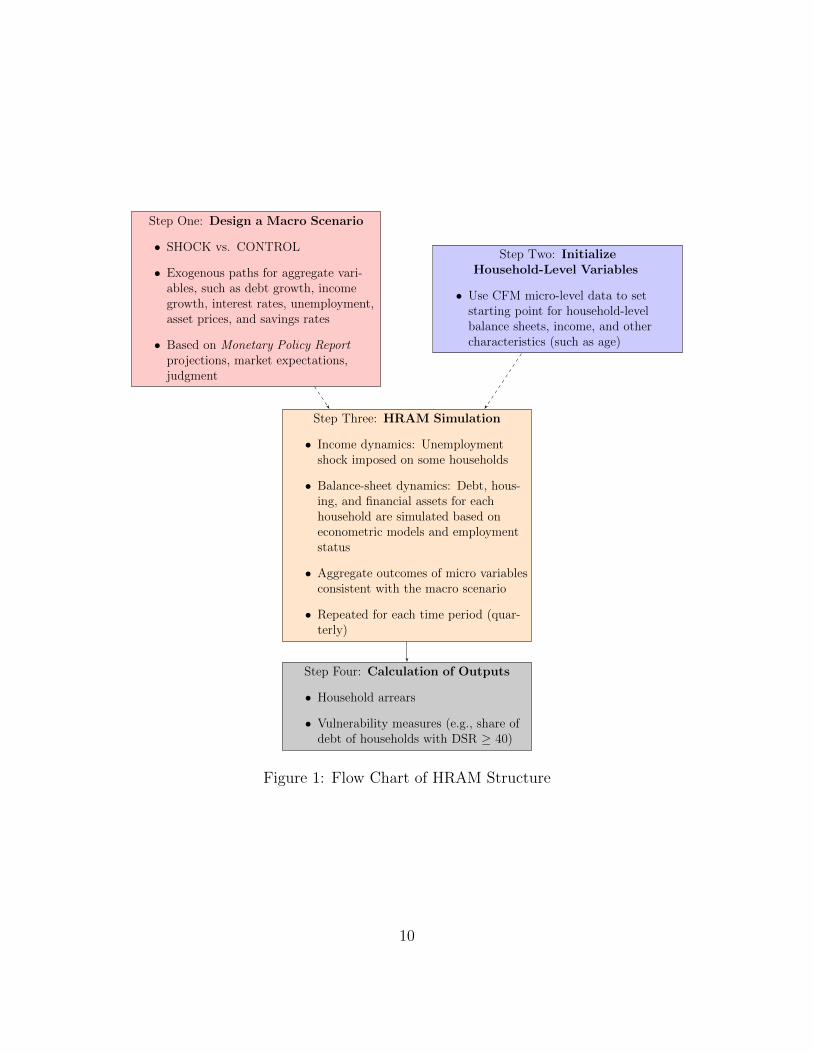
Four main steps are involved in running a simulation with HRAM: (i) the design of a
macroeconomic scenario exogenous to the model; (ii) the initialization of household
balance sheets using microdata; (iii) the simulation itself; and (iv) the calculation
of the output of the model. Figure 1 shows these steps, where steps one and two
are the inputs into the model. HRAM includes steps three and four, and leads to
the final calculation of aggregate measures of household vulnerabilities and arrears.
In the first step, the design of an exogenous macroeconomic scenario includes
a coherent set of assumptions for the paths of key macroeconomic variables such
as household debt growth, income growth, interest rates, and unemployment. Typ-
ically, an HRAM stress testing exercise includes both the shock scenario, and a
control case that provides a stable scenario as a reference point. The formulation
of the control-case assumptions can draw on projections from the Bank’s Monetary
Policy Report (MPR), market expectations for the overnight rate, and additional
judgment, for example. A shock scenario could be historically based, or not, and
could instead be more severe than what has been experienced in the past.5 For
other analysis, assumptions can be based on forecasts from other models such as
the Bank’s dynamic stochastic general-equilibrium model, ToTEM. Paths for the as-
sumptions are typically defined at a quarterly frequency for the simulation horizon
of 3-5 years. As highlighted earlier, the macro scenario can be designed to indirectly
capture general-equilibrium effects that cannot be explicitly modelled in HRAM.
The second step consists of initializing the balance sheets and other character-
istics (such as income and age) of a large number of heterogeneous households that
serve as the starting point of the simulation. The initialization is done using the lat-
est data from the Canadian Financial Monitor (CFM), which is a large micro-level
data set, covering over 12,000 households in a year.6 Some degree of simplification
is involved: for example, CFM survey respondents can list up to eight mortgages;
the HRAM set-up sums up any outstanding mortgage debt into one primary mort-
gage. Preliminary calculations are then performed – for example, the calculation of
household-specific risk premiums and missing values are addressed.
5Note that HRAM scenarios are separate from any evaluation of event probability and areillustrative of possible outcomes conditional on the scenario materializing – the focus generallybeing the stress testing of tail events that could pose a risk to financial and macroeconomic stability.
6This data set is discussed in more detail in Section 5.
9
Step One: Design a Macro Scenario
• SHOCK vs. CONTROL
• Exogenous paths for aggregate vari-ables, such as debt growth, incomegrowth, interest rates, unemployment,asset prices, and savings rates
• Based on Monetary Policy Reportprojections, market expectations,judgment
Step Two: InitializeHousehold-Level Variables
• Use CFM micro-level data to setstarting point for household-levelbalance sheets, income, and othercharacteristics (such as age)
Step Three: HRAM Simulation
• Income dynamics: Unemploymentshock imposed on some households
• Balance-sheet dynamics: Debt, hous-ing, and financial assets for eachhousehold are simulated based oneconometric models and employmentstatus
• Aggregate outcomes of micro variablesconsistent with the macro scenario
• Repeated for each time period (quar-terly)
Step Four: Calculation of Outputs
• Household arrears
• Vulnerability measures (e.g., share ofdebt of households with DSR ≥ 40)
Figure 1: Flow Chart of HRAM Structure
10
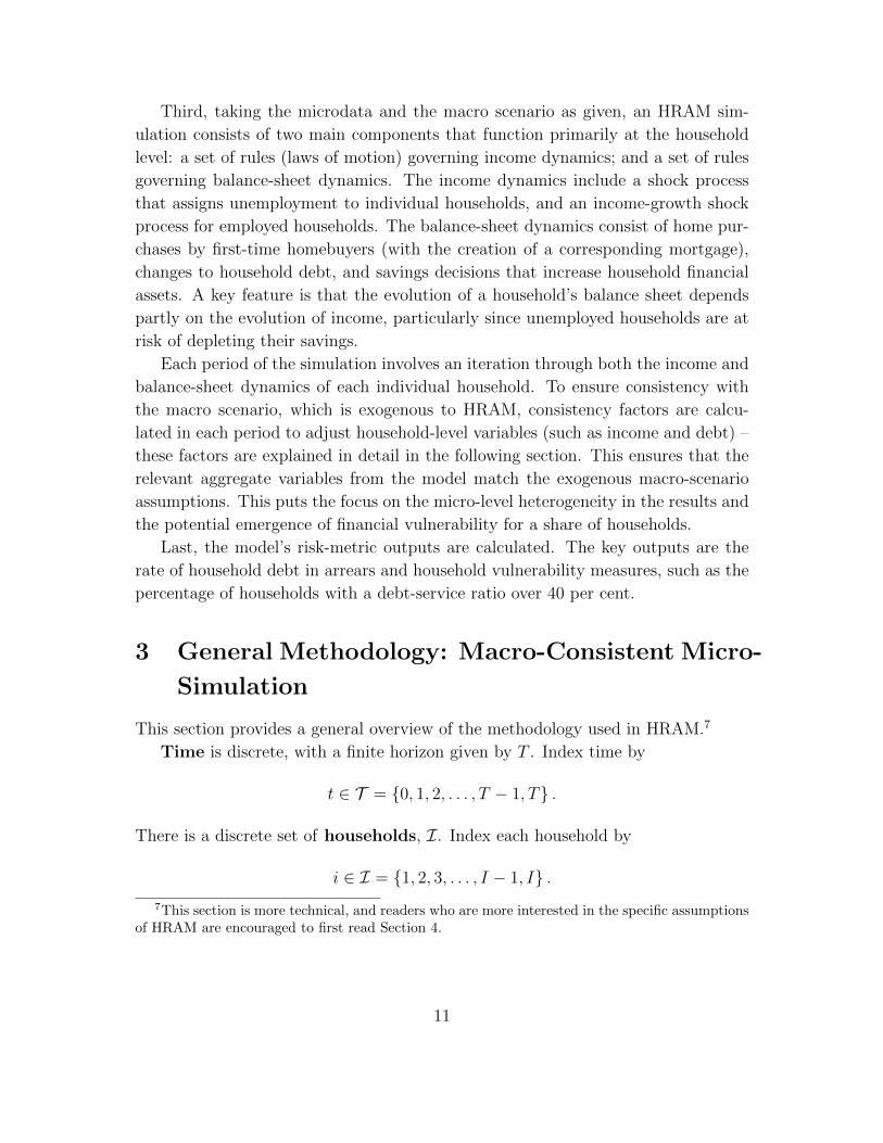
Third, taking the microdata and the macro scenario as given, an HRAM sim-
ulation consists of two main components that function primarily at the household
level: a set of rules (laws of motion) governing income dynamics; and a set of rules
governing balance-sheet dynamics. The income dynamics include a shock process
that assigns unemployment to individual households, and an income-growth shock
process for employed households. The balance-sheet dynamics consist of home pur-
chases by first-time homebuyers (with the creation of a corresponding mortgage),
changes to household debt, and savings decisions that increase household financial
assets. A key feature is that the evolution of a household’s balance sheet depends
partly on the evolution of income, particularly since unemployed households are at
risk of depleting their savings.
Each period of the simulation involves an iteration through both the income and
balance-sheet dynamics of each individual household. To ensure consistency with
the macro scenario, which is exogenous to HRAM, consistency factors are calcu-
lated in each period to adjust household-level variables (such as income and debt) –
these factors are explained in detail in the following section. This ensures that the
relevant aggregate variables from the model match the exogenous macro-scenario
assumptions. This puts the focus on the micro-level heterogeneity in the results and
the potential emergence of financial vulnerability for a share of households.
Last, the model’s risk-metric outputs are calculated. The key outputs are the
rate of household debt in arrears and household vulnerability measures, such as the
percentage of households with a debt-service ratio over 40 per cent.
3 General Methodology: Macro-Consistent Micro-
Simulation
This section provides a general overview of the methodology used in HRAM.7
Time is discrete, with a finite horizon given by T . Index time by
t ∈ T = 0, 1, 2, . . . , T − 1, T .
There is a discrete set of households, I. Index each household by
i ∈ I = 1, 2, 3, . . . , I − 1, I .7This section is more technical, and readers who are more interested in the specific assumptions
of HRAM are encouraged to first read Section 4.
11
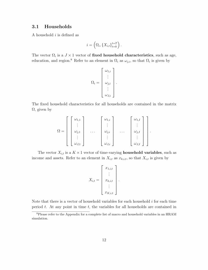
3.1 Households
A household i is defined as
i =(
Ωi, Xi,tt=Tt=0
).
The vector Ωi is a J × 1 vector of fixed household characteristics, such as age,
education, and region.8 Refer to an element in Ωi as ωj,i, so that Ωi is given by
Ωi =
ω1,i
...
ωj,i...
ωJ,i
.
The fixed household characteristics for all households are contained in the matrix
Ω, given by
Ω =
ω1,1
...
ωj,1...
ωJ,1
. . .
ω1,i
...
ωj,i...
ωJ,i
. . .
ω1,I
...
ωj,I...
ωJ,I
.
The vector Xi,t is a K× 1 vector of time-varying household variables, such as
income and assets. Refer to an element in Xi,t as xk,i,t, so that Xi,t is given by
Xi,t =
x1,i,t
...
xk,i,t...
xK,i,t
.
Note that there is a vector of household variables for each household i for each time
period t. At any point in time t, the variables for all households are contained in
8Please refer to the Appendix for a complete list of macro and household variables in an HRAMsimulation.
12
the matrix Xt, given by
Xt =
x1,1,t
...
xk,1,t...
xK,1,t
. . .
x1,i,t
...
xk,i,t...
xK,i,t
. . .
x1,I,t
...
xk,I,t...
xK,I,t
.
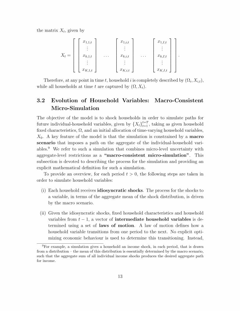
Therefore, at any point in time t, household i is completely described by (Ωi, Xi,t),
while all households at time t are captured by (Ω, Xt).
3.2 Evolution of Household Variables: Macro-Consistent
Micro-Simulation
The objective of the model is to shock households in order to simulate paths for
future individual-household variables, given by Xtt=Tt=1 , taking as given household
fixed characteristics, Ω, and an initial allocation of time-varying household variables,
X0. A key feature of the model is that the simulation is constrained by a macro
scenario that imposes a path on the aggregate of the individual-household vari-
ables.9 We refer to such a simulation that combines micro-level uncertainty with
aggregate-level restrictions as a “macro-consistent micro-simulation”. This
subsection is devoted to describing the process for the simulation and providing an
explicit mathematical definition for such a simulation.
To provide an overview, for each period t > 0, the following steps are taken in
order to simulate household variables:
(i) Each household receives idiosyncratic shocks. The process for the shocks to
a variable, in terms of the aggregate mean of the shock distribution, is driven
by the macro scenario.
(ii) Given the idiosyncratic shocks, fixed household characteristics and household
variables from t − 1, a vector of intermediate household variables is de-
termined using a set of laws of motion. A law of motion defines how a
household variable transitions from one period to the next. No explicit opti-
mizing economic behaviour is used to determine this transitioning. Instead,
9For example, a simulation gives a household an income shock, in each period, that is drawnfrom a distribution – the mean of this distribution is essentially determined by the macro scenario,such that the aggregate sum of all individual income shocks produces the desired aggregate pathfor income.
13
restrictions guided by economic theory, and estimated equations, are used to
approximate household decision making.
(iii) Given the intermediate household variables, the consistency of the path for
household variables with the macro scenario is ensured by solving for a vec-
tor of endogenous consistency factors that linearly adjust the variables to
restore consistency with the set of macro restrictions. The factors are de-
fined so as to adjust the variables proportionally for the relevant group of
households.10
(iv) The final household variables for period t are computed by updating the
intermediate household variables via an allocation function that uses the
consistency factors for this linear adjustment.
For instance, one household variable is income. Each household receives an idiosyn-
cratic shock to its income, but through the macro scenario there is a restriction
imposed on overall income growth across all households.
In the remainder of this subsection, we define a macro scenario, go over each
step in simulating household variables, and finally define a macro-consistent micro-
simulation.
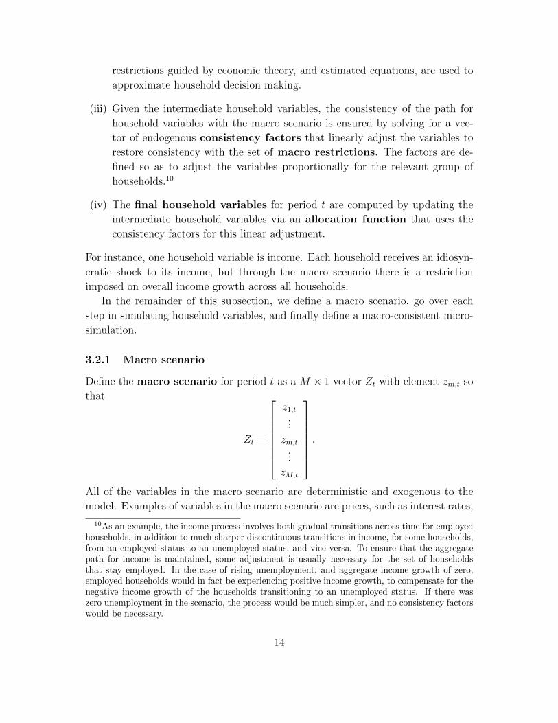
3.2.1 Macro scenario
Define the macro scenario for period t as a M × 1 vector Zt with element zm,t so
that
Zt =
z1,t
...
zm,t...
zM,t
.
All of the variables in the macro scenario are deterministic and exogenous to the
model. Examples of variables in the macro scenario are prices, such as interest rates,
10As an example, the income process involves both gradual transitions across time for employedhouseholds, in addition to much sharper discontinuous transitions in income, for some households,from an employed status to an unemployed status, and vice versa. To ensure that the aggregatepath for income is maintained, some adjustment is usually necessary for the set of householdsthat stay employed. In the case of rising unemployment, and aggregate income growth of zero,employed households would in fact be experiencing positive income growth, to compensate for thenegative income growth of the households transitioning to an unemployed status. If there waszero unemployment in the scenario, the process would be much simpler, and no consistency factorswould be necessary.
14
and other macroeconomic variables such as aggregate nominal income growth and
the unemployment rate.11 The complete macro scenario for all time periods is given
by the following matrix:
Z = [Z0, Z1, Z2, . . . , ZT−1, ZT ] .
The macro scenario must be chosen before the simulation is performed and is part
of the initialization of the simulation. Typically, the macro scenario is constructed
to be consistent with a dynamic general-equilibrium model. Mathematically, the
macro scenario is a set of M restrictions for each period t on the path of household
variables given by Xtt=Tt=1 .
3.2.2 Idiosyncratic shocks
Let εi,t be a K × 1 vector of idiosyncratic shocks with element εk,i,t, so that
εi,t =
ε1,i,t
...
εk,i,t...
εK,i,t
.
The shocks are stochastic and are drawn from a distribution (e.g., normal or gamma).
Typically, the mean and variance of the shocks will vary with the fixed household
characteristics of household i, the macro scenario for both t and t − 1, the distri-
bution of households across household variables in the previous period, and a set
of parameters Θε that affect the distribution functions. Therefore, we write the
shocks as being drawn from a cumulative distribution function, F , that depends
upon household i fixed characteristics, the past aggregate economy via Xt−1, and
the macro scenario via Zt and Zt−1:
εi,t ∼ F (Ωi;Xt−1, Zt, Zt−1; Θε) . (1)
The underlying distributions for each element of εi,t (i.e., such as normal or uniform),
as well as the vector of parameters, Θε, are determined in the calibration stage
and are fixed throughout the simulation. The matrix for all the shocks across all
11Please refer to the Appendix for a complete list of macro and household variables in an HRAMsimulation.
15
households at time t is expressed as
εt =
ε1,1,t
...
εk,1,t...
εK,1,t
. . .
ε1,i,t
...
εk,i,t...
εK,i,t
. . .
ε1,I,t
...
εk,I,t...
εK,I,t
.
3.2.3 Intermediate household variables: Law of motion
Given the idiosyncratic shocks, intermediate values for all household variables for
household i, denoted as Xi,t, are updated via the following function:
Xi,t = G (Xi,t−1, εi,t) . (2)
Note that equation (2) depends only upon household-level variables, and through
the idiosyncratic shocks, the aggregate of the variables, and the macro scenario.
Refer to the function G as the law of motion for household variables. A central
element of the model is the construction of the law of motion for each household
variable, detailed in Section 4. For certain specific household variables, such as
income, the law of motion involves the interaction of more than one idiosyncratic
shock per period, i.e., there is a process for fully employed households, as well as
transitions from an employed status to an unemployed status, and vice versa.
3.2.4 Consistency factors: Macro restrictions
The evolution of the household variables is refined by a set of time-varying M ×1 vector Ct of consistency factors. These are endogenous factors that ensure
that the evolution of the household variables is consistent with the macro scenario.
Formally, the M×1 restrictions from the macro scenario are captured in the function
H, given by
Ct = H(Xt, Xt−1, Zt, Zt−1
). (3)
Note that equation (3) consists of M restrictions on the aggregate household vari-
ables. Refer to H as the function of macro restrictions. The specific definitions
of the consistency factors for each specific household variable will be explained in
the relevant subsections.
16
3.2.5 Final household variables: Allocation function
Given the consistency factors, the temporary household variables for a household i
at time t are updated by the function G to arrive at the final household variables:
Xi,t = G(Xi,t, Xt, Ct; εi,t
). (4)
Refer to the function G as the allocation function. If the functions H and G have
been appropriately constructed, then
H (Xt, Xt−1, Zt, Zt−1) = 0.
3.2.6 Definition of a macro-consistent micro-simulation
A macro-consistent micro-simulation is defined as follows.
Definition 1. A macro-consistent micro-simulation consists of sequences,
εtt=Tt=1 ,Xt
t=Tt=1
, Ctt=Tt=1 and Xtt=Tt=1 such that, given X0, Ω,and Z:
(i) (Idiosyncratic shocks) εi,t satisfies equation (1) for each i ∈ I and t ∈ 1, ..., T;
(ii) (Evolution of intermediate household variables) Xi,t satisfies equation (2) for
each i ∈ I and t ∈ 1, ..., T;
(iii) (Macro consistency) Ct satisfies equation (3) for each t ∈ 1, ..., T; and
(iv) (Evolution of final household variables) Xi,t satisfies equation (4) for each i ∈ Iand t ∈ 1, ..., T.
4 The Model
This section covers the primary equations behind HRAM. The first subsection dis-
cusses the evolution of income and employment at the household level and illustrates
how the aggregate evolution of income and employment in the model is constrained
by the macro scenario. The second subsection covers the evolution of individual
household balance sheets, including the determination of whether a household will
purchase a house for the first time and whether a household will go into arrears on its
debt. Once again, a key feature is how the evolution of the aggregate balance sheet
for the total household sector is constrained by the macro scenario. A complete list
of all of the variables used is provided in Appendix A.
17
4.1 Evolution of Income and Employment
The disposable nominal labour income of household i in period t, denoted as
XDLYi,t , is a function of a household’s fully employed permanent nominal labour
income in period t, XPLYi,t , and whether a household is unemployed in period
t.12 Letting XUi,t = 0 denote that household i is employed in period t, and XU
i,t = 1
denote that household i is unemployed in period t, the disposable labour income of
household i in period t is given by:
XDLYi,t = (1− τ)
(XPLYi,t − (1− b)XU
i,tXPLYi,t
), (5)
where b denotes the percentage of permanent labour income that a household re-
ceives while unemployed (from unemployment compensation) and τ denotes the tax
rate on labour income.
An individual household i faces three sources of uncertainty in its income process:
(i) whether a household is employed or unemployed; (ii) while unemployed, the
duration of unemployment; and (iii) uncertainty in its permanent labour income,
which denotes income while employed.
In the aggregate, the macro scenario dictates the overall unemployment rate
in period t, ZUt ; the expected duration of unemployment for a household that
becomes unemployed in period t, ZUDt ; and the overall nominal growth rate in
labour income from t− 1 to t, ZLY Gt .
4.1.1 Unemployment and unemployment duration
When a household becomes unemployed in period t, it receives an unemployment
duration shock, εUDi,t , that determines the duration13 (number of periods) of unem-
ployment for household i. Let XUDi,t denote the expected remaining unemployment
duration for household i at the end of period t. Therefore, at the start of period t,
the number of households that continue to be unemployed is given by
IUDt−1 =i=I∑i=1
Ind(XUDi,t−1 > 0
),
12With some abuse of terminology, we define permanent labour income to be what a householdwould earn in a fully employed state, ignoring any temporary effects from unemployment, whichis the main source of the transitory component to current disposable income, in the model.
13More precisely, this is the maximum duration of the unemployment episode for the householdsince it can receive a shock and become employed before its remaining period of unemployment goesto zero. This possibility can exist if the unemployment rate in the macro scenario falls abruptly.
18
where Ind denotes an indicator function that is equal to one if, and only if, the ar-
gument is true, and zero otherwise. The macro scenario dictates that the aggregate
unemployment rate should be equal to ZUt . The difference between the unemploy-
ment rate in the macro scenario and the implied unemployment rate in period t
from households with continuing unemployment is given by14
pt = ZUt −
IUDt−1
I.
Let pi,t denote the probability that household i, employed in period t − 1,
XUDt−1 = 0, will become unemployed in period t. Let qt denote the probability that a
household unemployed in period t− 1 with a strictly positive remaining duration of
unemployment, XUDt−1 > 0, will become employed.15 The values for the two proba-
bilities are determined by p, and, in the case of pi,t, a relative layoff risk factor ϕi,t,
which is a function of the vector of fixed household-specific characteristics, Ωi, and
the employment status of households in period t− 1, XUDi,t−1
16,17:
pi,t = max
0,
ptI
I − IUDt−1
ϕ(Ωi,t, XUDi,t−1)
and qt = max
0,− ptI
IUDt−1
,
where ϕ is defined such that it has mean equal to one for households employed in
period t− 1.
Formally, let εUi,t denote a shock uniformly distributed over [0, 1]. Whether a
household is employed or unemployed in period t depends upon XUDi,t−1, εUi,t, pi,t and
14Note that we describe the unemployment rate as relative to the total number of households, I,for simplicity of exposition. In the actual model, we examine the employment of heads of householdrelative to the labour force, controlling for labour force status when we initialize the model fromdata.
15Note that even though qt is typically zero, there are still gross flows of unemployment owingto the duration shock, since the households that end their unemployment spell have to be replacedwith other households in order to maintain a constant rate of unemployment. For instance, in atypical labour-search model, qt refers to the probability that an unemployed agent finds work ina given period and is always strictly positive. Here, qt refers to households that unexpectedly endtheir unemployment spell early.
16The estimation of ϕi,t is explained further in Section 6.17As can be seen from equation (6), qt, and thus the duration of a household unemployment
spell, does not depend on Ωi in the model.
19
qt by the following function, with XUi,t = 1 indicating unemployment:
XUi,t =
1 if XUD
i,t−1 = 0 and εUi,t ≤ pi,t
0 if XUDi,t−1 = 0 and εUi,t > pi,t
1 if XUDi,t−1 > 0 and εUi,t > qt
0 if XUDi,t−1 > 0 and εUi,t ≤ qt
. (6)
By construction, the process for unemployment ensures that the unemployment rate
from the macro scenario is exactly matched (assuming that there is a sufficient num-
ber of households to ensure that the law of large numbers holds) so that consistency
factors are not needed in the unemployment process for households.
After the employment status for a household is determined, the remaining un-
employment duration for unemployed households has to be updated. For those
households that are in the middle of an unemployment spell, the remaining dura-
tion is simply reduced by a period. Households that are newly unemployed draw a
shock that determines the duration of their unemployment spell. Formally, the law
of motion for XUDi,t is given by
XUDi,t =
XUDi,t−1 − 1 if XU
i,t = 1 and XUDi,t−1 > 0
εUDi,t − 1 if XUi,t = 1 and XUD
i,t−1 = 0
0 if XUi,t = 0
. (7)
The idiosyncratic shock εUDi,t is the unemployment duration shock for a household
that became unemployed in period t. The distribution of this shock is given by FUD
and the expected duration of unemployment depends upon the macro-scenario
variable ZUDt , so that
εUDi,t ∼ FUD(ZUDt
),
where the mean of the distribution is determined by ZUDt . The cumulative dis-
tribution function, FUD, captures the fact that many households that become un-
employed find work quickly,18 while other households remain unemployed for an
extended period of time. The specifics are covered in Section 6 on estimation and
calibration.
18The structure allows for some households to be unemployed for only one period.
20
4.1.2 Permanent labour income
The law of motion for the permanent labour income of household i at time t is given
by
XPLYi,t = XPLY
i,t−1
(1 + εPLYi,t
)+ CLY G
i,t , (8)
where εPLYi,t is an idiosyncratic shock to permanent labour income for household
i at time t. A consistency factor, CLY Gi,t , ensures that the aggregate growth from
the idiosyncratic labour-income shocks is consistent with the nominal growth rate
of aggregate labour income from the macro scenario, ZLY Gt . The next paragraphs
cover first the idiosyncratic shock followed by the determination of the consistency
factor.
Households that are employed in period t receive a shock that affects the growth
rate of their income, εPLYi,t . This shock is distributed normally, with the mean
given by the macro scenario and standard deviation σPLYi that is a function of
the household’s income quintile, ωY Qi .19 Unemployed households’ permanent labour
income remains unchanged. Formally, the process for household i’s idiosyncratic
shock to permanent labour income at time t is given by
εPLYi,t =
∼ N(ZLY Gt , σPLY (ωY Qi )
)if XU
i,t = 0
0 if XUi,t = 1
. (9)
Turning to the determination of the consistency factor, the idiosyncratic shock
generates an intermediate household variable for permanent labour income:
XPLYi,t = XPLY
i,t−1
(1 + εPLYi,t
).
The aggregate nominal labour income in period t− 1 is given by
LYt−1 =I∑i
[XPLYi,t−1 − (1− b)XU
i,t−1XPLYi,t−1
].
From the macro scenario, ZLY Gt denotes the growth rate in aggregate nominal labour
income from period t − 1 to t, so that aggregate nominal labour income in period
t should be equal to(1 + ZLY G
t
)LYt−1. Given XPLY
t and XUt , a consistency factor
CLY Gt is calculated that ensures that aggregate nominal income growth matches the
19See Djoudad (2012) for further details.
21
macro scenario:
CLY Gt =
(1 + ZLY G
t
)LYt−1 −
I∑i
[XPLYi,t − (1− b)XU
i,tXPLYi,t
].
This captures the aggregate amount of income that has to be added to (or subtracted
from if negative) employed households in order to match the macro scenario. The
consistency factor CLY Gt is allocated across employed households in proportion to
their share of the income-growth shock, such that the share of the income-growth
shock does not change for any household, to arrive at a final consistency adjustment
to household permanent nominal income for period t:
CLY Gi,t =
Ind(XUi,t = 0
)XPLYi,t−1ε
PLYi,t∑I
i Ind(XUi,t = 0
)XPLYi,t−1ε
PLYi,t
CLY Gt . (10)
4.2 Evolution of Household Balance Sheet
Given the shocks to unemployment, permanent labour income, and the return on
financial assets, the total financial resources available to a household, which we
refer to as a household’s budget, is the sum of realized gross income (minus tax
payments) and financial assets (with the return) less debt. In addition, households
are assumed to make their required debt payments if they have sufficient resources
to cover them (while still maintaining a minimal level of consumption if a household
is unemployed).
To add clarification, the allocation of a household’s assets, debt, and consump-
tion is captured by the household budget constraint in period t:
XFAi,t −XD
i,t +XCi,t︸ ︷︷ ︸
Assets, debt, consumption
= XPLYi,t (1− τ) +XFA
i,t−1
(1 + ZRFA
t
)−XD
i,t−1︸ ︷︷ ︸Available financial resources
− XDPi,t︸ ︷︷ ︸
Required debt payments
,
where τ is the tax rate on income, and ZRFAt is the return on financial assets, which
is part of the macro scenario.
To determine the allocation across consumption, and next period’s debt and
assets, no explicit modelling of behaviour is used. Instead, stochastic processes that
provide a reduced-form representation of economic decision making by incorporating
household variables and fixed household characteristics determine debt and assets for
subsequent periods, with household consumption being given by the residual term.
In the rest of this subsection, we go over the determination of debt, assets (both
financial and whether a renting household buys a house), and whether a household
22
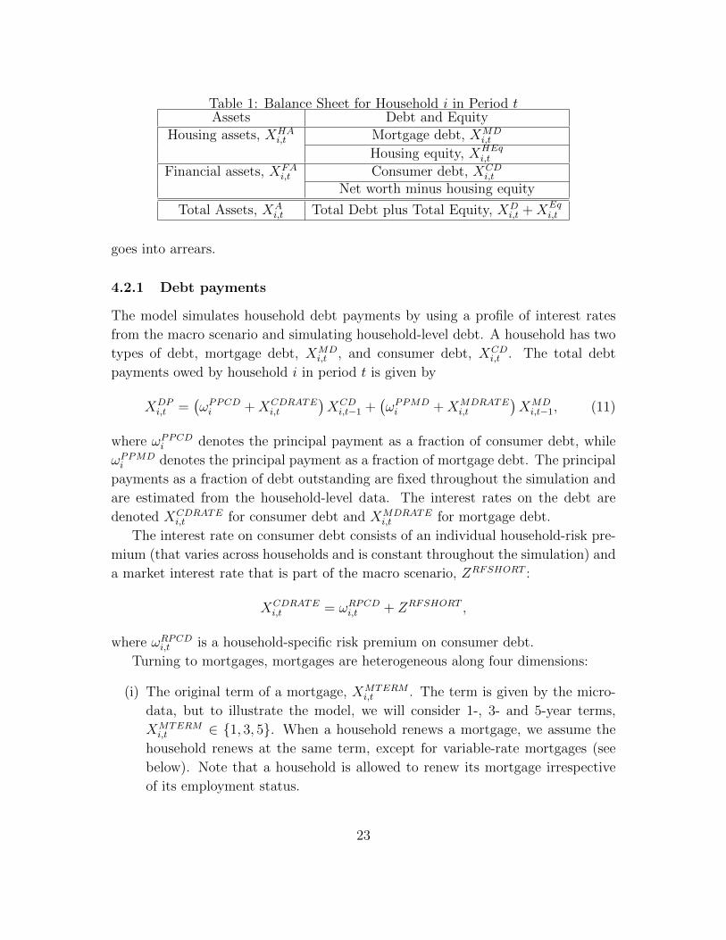
Table 1: Balance Sheet for Household i in Period tAssets Debt and Equity
Housing assets, XHAi,t Mortgage debt, XMD
i,t
Housing equity, XHEqi,t
Financial assets, XFAi,t Consumer debt, XCD
i,t
Net worth minus housing equity
Total Assets, XAi,t Total Debt plus Total Equity, XD
i,t +XEqi,t
goes into arrears.
4.2.1 Debt payments
The model simulates household debt payments by using a profile of interest rates
from the macro scenario and simulating household-level debt. A household has two
types of debt, mortgage debt, XMDi,t , and consumer debt, XCD
i,t . The total debt
payments owed by household i in period t is given by
XDPi,t =
(ωPPCDi +XCDRATE
i,t
)XCDi,t−1 +
(ωPPMDi +XMDRATE
i,t
)XMDi,t−1, (11)
where ωPPCDi denotes the principal payment as a fraction of consumer debt, while
ωPPMDi denotes the principal payment as a fraction of mortgage debt. The principal
payments as a fraction of debt outstanding are fixed throughout the simulation and
are estimated from the household-level data. The interest rates on the debt are
denoted XCDRATEi,t for consumer debt and XMDRATE
i,t for mortgage debt.
The interest rate on consumer debt consists of an individual household-risk pre-
mium (that varies across households and is constant throughout the simulation) and
a market interest rate that is part of the macro scenario, ZRFSHORT :
XCDRATEi,t = ωRPCDi,t + ZRFSHORT ,
where ωRPCDi,t is a household-specific risk premium on consumer debt.
Turning to mortgages, mortgages are heterogeneous along four dimensions:
(i) The original term of a mortgage, XMTERMi,t . The term is given by the micro-
data, but to illustrate the model, we will consider 1-, 3- and 5-year terms,
XMTERMi,t ∈ 1, 3, 5. When a household renews a mortgage, we assume the
household renews at the same term, except for variable-rate mortgages (see
below). Note that a household is allowed to renew its mortgage irrespective
of its employment status.
23
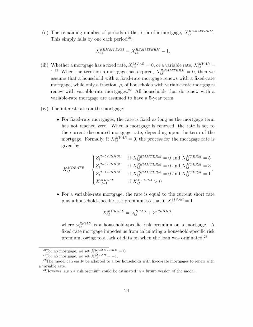
(ii) The remaining number of periods in the term of a mortgage, XREMMTERMi,t .
This simply falls by one each period20:
XREMMTERMi,t = XREMMTERM
i,t − 1.
(iii) Whether a mortgage has a fixed rate, XMVARi,t = 0, or a variable rate, XMVAR
i,t =
1.21 When the term on a mortgage has expired, XREMMTERMi,t = 0, then we
assume that a household with a fixed-rate mortgage renews with a fixed-rate
mortgage, while only a fraction, ρ, of households with variable-rate mortgages
renew with variable-rate mortgages.22 All households that do renew with a
variable-rate mortgage are assumed to have a 5-year term.
(iv) The interest rate on the mortgage:
• For fixed-rate mortgages, the rate is fixed as long as the mortgage term
has not reached zero. When a mortgage is renewed, the rate is set to
the current discounted mortgage rate, depending upon the term of the
mortgage. Formally, if XMVARi,t = 0, the process for the mortgage rate is
given by
XMDRATEi,t =
ZR−5Y RDISCt if XREMMTERM
i,t = 0 and XMTERMi,t = 5
ZR−3Y RDISCt if XREMMTERM
i,t = 0 and XMTERMi,t = 3
ZR−1Y RDISCt if XREMMTERM
i,t = 0 and XMTERMi,t = 1
XMRATEi,t−1 if XMTERM
i,t > 0
.
• For a variable-rate mortgage, the rate is equal to the current short rate
plus a household-specific risk premium, so that if XMVARi,t = 1
XMDRATEi,t = ωRPMD
i,t + ZRSHORT ,
where ωRPMDi,t is a household-specific risk premium on a mortgage. A
fixed-rate mortgage impedes us from calculating a household-specific risk
premium, owing to a lack of data on when the loan was originated.23
20For no mortgage, we set XREMMTERMi,t = 0.
21For no mortgage, we set XMVARi,t = −1.
22The model can easily be adapted to allow households with fixed-rate mortgages to renew witha variable rate.
23However, such a risk premium could be estimated in a future version of the model.
24
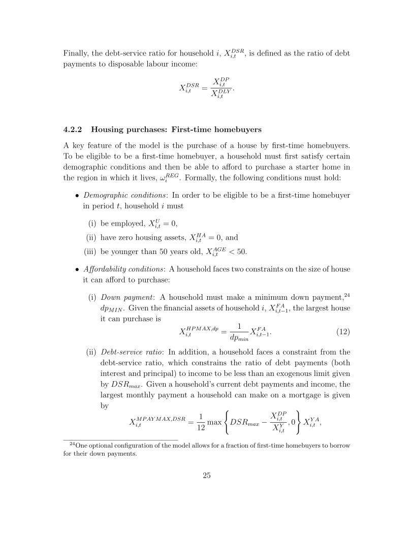
Finally, the debt-service ratio for household i, XDSRi,t , is defined as the ratio of debt
payments to disposable labour income:
XDSRi,t =
XDPi,t
XDLYi,t
.
4.2.2 Housing purchases: First-time homebuyers
A key feature of the model is the purchase of a house by first-time homebuyers.
To be eligible to be a first-time homebuyer, a household must first satisfy certain
demographic conditions and then be able to afford to purchase a starter home in
the region in which it lives, ωREGi . Formally, the following conditions must hold:
• Demographic conditions : In order to be eligible to be a first-time homebuyer
in period t, household i must
(i) be employed, XUi,t = 0,
(ii) have zero housing assets, XHAi,t = 0, and
(iii) be younger than 50 years old, XAGEi,t < 50.
• Affordability conditions : A household faces two constraints on the size of house
it can afford to purchase:
(i) Down payment : A household must make a minimum down payment,24
dpMIN . Given the financial assets of household i, XFAi,t−1, the largest house
it can purchase is
XHPMAX,dpi,t =
1
dpminXFAi,t−1. (12)
(ii) Debt-service ratio: In addition, a household faces a constraint from the
debt-service ratio, which constrains the ratio of debt payments (both
interest and principal) to income to be less than an exogenous limit given
by DSRmax. Given a household’s current debt payments and income, the
largest monthly payment a household can make on a mortgage is given
by
XMPAYMAX,DSRi,t =
1
12max
DSRmax −
XDPi,t
XYi,t
, 0
XY Ai,t ,
24One optional configuration of the model allows for a fraction of first-time homebuyers to borrowfor their down payments.
25
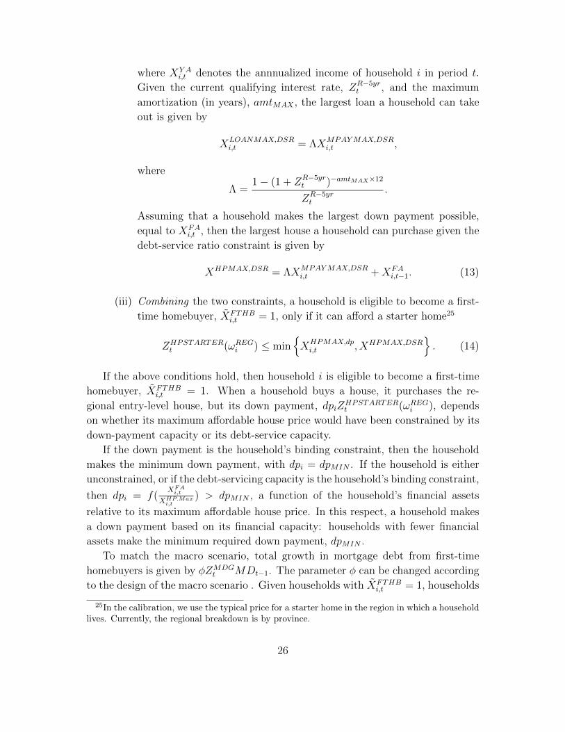
where XY Ai,t denotes the annnualized income of household i in period t.
Given the current qualifying interest rate, ZR−5yrt , and the maximum
amortization (in years), amtMAX , the largest loan a household can take
out is given by
XLOANMAX,DSRi,t = ΛXMPAYMAX,DSR
i,t ,
where
Λ =1− (1 + ZR−5yr
t )−amtMAX×12
ZR−5yrt
.
Assuming that a household makes the largest down payment possible,
equal to XFAi,t , then the largest house a household can purchase given the
debt-service ratio constraint is given by
XHPMAX,DSR = ΛXMPAYMAX,DSRi,t +XFA
i,t−1. (13)
(iii) Combining the two constraints, a household is eligible to become a first-
time homebuyer, XFTHBi,t = 1, only if it can afford a starter home25
ZHPSTARTERt (ωREGi ) ≤ min
XHPMAX,dpi,t , XHPMAX,DSR
. (14)
If the above conditions hold, then household i is eligible to become a first-time
homebuyer, XFTHBi,t = 1. When a household buys a house, it purchases the re-
gional entry-level house, but its down payment, dpiZHPSTARTERt (ωREGi ), depends
on whether its maximum affordable house price would have been constrained by its
down-payment capacity or its debt-service capacity.
If the down payment is the household’s binding constraint, then the household
makes the minimum down payment, with dpi = dpMIN . If the household is either
unconstrained, or if the debt-servicing capacity is the household’s binding constraint,
then dpi = f(XFA
i,t
XHP.Maxi,t
) > dpMIN , a function of the household’s financial assets
relative to its maximum affordable house price. In this respect, a household makes
a down payment based on its financial capacity: households with fewer financial
assets make the minimum required down payment, dpMIN .
To match the macro scenario, total growth in mortgage debt from first-time
homebuyers is given by φZMDGt MDt−1. The parameter φ can be changed according
to the design of the macro scenario . Given households with XFTHBi,t = 1, households
25In the calibration, we use the typical price for a starter home in the region in which a householdlives. Currently, the regional breakdown is by province.
26
are randomly drawn, setting XFTHB = 1 until∑i
XFTHBi,t ZHPSTARTER
t (ωREGi )(1− dpi) ≥ φZMDGt MDt−1.
If an eligible household is assigned as a first-time homebuyer, XFTHBi,t = 1, then
its debt payments are based on the discounted 5-year mortgage rate, ZR−5yr−disct ,
rather than the qualifying (posted) rate, ZR−5yrt .26
4.2.3 Mortgage debt: Non-first-time homebuyers
• If a household is employed, then an intermediate variable for mortgage debt
is generated by the following law of motion:
log XMDi,t = logXMD
i,t−1 + αCNSMD +(1− λMDInd
(XDSRi,t > 40
))×[
αY GMD∆logXPLYi,t + αRMD∆ZR−5Y RDISC
t + αHPMDZHPGt XHA
t−1
]+ εMD
i,t , (15)
where ZHPGt is the nominal growth in aggregate house prices given by the
macro scenario. The distribution of the error term is given by
εMDi,t ∼ FMD.
Therefore, mortgage debt depends upon the change in income for a household,
as well as the change in interest rates and the increase in house prices. The
λ coefficient captures a non-linearity where a debt-service ratio over 40 lowers
the growth in mortgage debt. In addition, there is an idiosyncratic shock that
affects mortgage debt. The details for the estimation behind the calibrated
values for the parameters are covered in Djoudad (2012). This specification
captures the ability of households to borrow against the rising value of their
homes.
• If a household is unemployed and has strictly positive mortgage debt, then
XMDi,t = XMD
i,t−1.
• If a household has no mortgage debt, then they may accumulate mortgage debt
according to the process for first-time homebuyers detailed in the previous
section.
26In practice, the qualifying rate can be defined to equal the discounted rate, which is the casein Canada for borrowers that opt for a 5-year fixed-rate mortgage.
27
• The aggregate realized mortgage debt in period t− 1 is given by
MDt−1 =I∑i
XMDi,t−1.
From the macro scenario, ZMDGt denotes the growth rate in mortgage debt
from period t − 1 to t, so that mortgage debt in period t should be equal to(1 + ZMDG
t
)MDt−1. However, only 1−φ per cent of mortgage debt growth is
assumed to be due to households with an existing mortgage. Therefore, given
XMDt , a consistency factor CMDG
t is calculated that will be used to make sure
that aggregate mortgage debt growth matches the macro scenario:
CMDGt =
(1 + (1− φ)ZMDG
t
)MDt−1 −
I∑i
XMDi,t .
This captures the aggregate amount of mortgage debt that has to be added
to (or subtracted from if negative) employed households that previously had
mortgage debt in order to match the macro scenario.
• The consistency factor CMDGt is allocated across employed households pro-
portionally based upon holdings of mortgage debt to arrive at final household
mortgage debt for period t:
XMDi,t = XMD
i,t +Ind
(XUi,t = 0
)(XMD
i,t −XMDi,t−1)∑I
i Ind(XUi,t = 0
)(XMD
i,t −XMDi,t−1)
CMDGt .
4.2.4 Consumer debt
• If a household is employed and had consumer debt in the previous period(XCDi,t−1 > 0
), then an intermediate variable for consumer debt is generated by
the following law of motion:
log XCDi,t = logXCD
i,t−1 + αCNSCD +(1− λCDInd
(XDSRi,t > 40
))×[
αY GCD∆logXYi,t + αRCD∆ZRCD
t + αHPMDZHPGt XHA
t−1
]+ εCDi,t , (16)
with the distribution of the error term given by
εCDi,t ∼ FCD.
28
The λCD coefficient captures a non-linearity where a debt-service ratio over
40 lowers the growth in consumer debt. In addition, there is an idiosyncratic
shock that affects consumer debt. The details for the estimation behind the
calibrated values for the parameters are covered in Djoudad (2012):
• Unemployed households are not allocated additional consumer debt through
the law of motion in equation 16,
XCDi,t = XCD
i,t−1.
• If a household has no consumer debt, then a household does not acquire any
consumer debt:
XCDi,t = 0.
An exception to this in the model is that an unemployed household can access
existing lines of credit to lessen the impacts of a temporary spell of unemploy-
ment. See subsection 4.2.7.
• The aggregate realized consumer debt in period t− 1 is given by
CDt−1 =I∑i
XCDi,t−1.
From the macro scenario, ZCDGt denotes the growth rate in consumer debt
from period t − 1 to t, so that consumer debt in period t should be equal to(1 + ZCDG
t
)CDt−1. Given XCD
t , a consistency factor CCDGt is calculated to
make sure that aggregate consumer debt growth matches the macro scenario:
CCDGt =
(1 + ZCDG
t
)CDt−1 −
I∑i
XCDi,t .
This captures the aggregate amount of consumer debt that has to be added
to (or subtracted from if negative) employed households in order to match the
macro scenario.
• The consistency factor CCDGt is allocated across employed households propor-
tionally, based upon holdings of consumer debt to arrive at final household
consumer debt for period t:
XCDi,t = XCD
i,t +Ind
(XUi,t = 0
)· (XCD
i,t −XCDi,t−1)∑I
i Ind(XUi,t = 0
)· (XCD
i,t −XCDi,t−1)
CCDGt .
29
4.2.5 Evolution of housing assets
For households with strictly positive housing assets, housing assets grow with house
prices:
XHAi,t =
(1 + ZHPG
t
)XHAi,t−1,
where ZHPGt denotes aggregate growth in nominal house values.
4.2.6 Savings: Accumulation of financial assets
Employed households are assumed to consume a fraction ωMPCi of their disposable
labour income. This generates an intermediate value for savings, after also subtract-
ing debt payments:
XSAVi,t =
(1− ωMPC
i
)XDLYi,t −XDP
i,t .
Unemployed households are assumed to consume a minimum, based on their perma-
nent labour income, XCi,t = κXPLY
i,t . Therefore, savings for unemployed households
are given by
XSAVi,t = XDLY
i,t − κXPLYi,t −XDP
i,t .
Note that unemployed households can have negative savings. We assumed earlier
that unemployed households do not increase borrowing, except in the special case
of existing lines of credit (see subsection 4.2.7), so that the negative savings of
unemployed households will result in a drawdown of their financial assets.
The consistency factor for savings is given by
CSAVt = ZSAV
t
I∑i
XDLYi,t −
I∑i
XSAVi,t ,
where ZSAVt is the aggregate savings rate coming from the macro scenario. The
consistency factor is then reallocated to employed households:
XSAV = XSAVi,t +
Ind(XUi,t = 0
)XSAVi,t∑I
i Ind(XUi,t = 0
)XSAVi,t
CSAVt .
Financial assets are then given by the combination of savings and asset returns:
XFAi,t = XFA
i,t−1
(1 + Ind
(XFAi,t−1 > 0
)ZRFAt
)+XSAV
i,t .
30
We allow for the asset returns to depend upon whether financial assets are positive
or negative by using an indicator function. This is done because we allow for the
possibility of financial assets to be negative, which we then use as an indicator of
a household being in arrears on its debt payments (see below). Note that because
of the way savings are structured, a household can only have negative savings,
and negative financial assets, if it cannot afford its debt payments. Therefore, the
amount by which debt is in arrears is given by negative financial assets.
4.2.7 Lines of credit
If a household is unemployed and has depleted its financial assets to zero, it can
draw on any unused credit room under its lines of credit to cover any dissavings
during the period. The initial availability of lines of credit and any unused room are
determined from the microdata. If credit room is insufficient, or if financial assets
have not yet reached zero, there is no draw:
XLC−Drawi,t =
−XSAV
i,t Ind(XSAVi,t−1 < 0
)if XLC
i,t−1 < XLC−Maxi +XSAV
i,t−1
and XFAi,t−1 = 0 and XUD
i,t−1 > 0
0 if XLCi,t−1 ≥ XLC−Max
i +XSAVi,t−1
or XFAi,t−1 > 0
.
Consumer debt and credit room under the lines of credit are updated accordingly:
XCDi,t = XCD
i,t−1 +XLC−Drawi,t .
XLCi,t = XLC
i,t−1 +XLC−Drawi,t .
When sufficient credit room to cover any dissavings is not available, a household is
susceptible to going into arrears.
4.2.8 Arrears
If financial assets turn negative, then a household is in arrears:
XARRi,t =
1 if XFA
i,t < 0
0 if XFAi,t ≥ 0
.
31
The number of consecutive periods that a household has been in arrears in its debt
payments is denoted by XCONARRi,t . The law of motion for XCONARR
i,t is given by
XCONARRi,t =
XCONARRi,t + 1 if XFA
i,t < 0
0 if XFAi,t ≥ 0
.
This variable can be used to construct measures of how long a household has been
in debt. For instance, in a quarterly model, if XCONARRi,t ≥ 1, then a household is 90
days or more in arrears, whereas in a monthly model, XCONARRi,t ≥ 3 would indicate
90 days or more in arrears. Given the structure of the model, a household can come
out of arrears only if it raises its financial assets back to positive.27
5 Data
Data to set up the starting point of HRAM’s household variables come from the
Canadian Financial Monitor (CFM), a survey compiled by Ipsos Reid. The data
include information on balance sheets, income, debt payments, and other financial
characteristics for about 12,000 households per year. The CFM data are weighted to
be cross-sectionally representative of the Canadian population, but most households
have taken part in the survey on more than one occasion.28 Given HRAM’s goal
of assessing household vulnerabilities over the simulation horizon, a discussion of
vulnerabilities as they appear at a relatively recent point in time is an apt starting
point for describing the data set. We use 2013 data to avoid any confusion with
more recent analyses of vulnerabilities that have appeared in the Financial System
Review, such as in Cateau, Roberts, and Zhou (2015).
A household’s debt payment burden is typically characterized relative to its
income, to give a debt-service ratio (DSR) of debt payments divided by gross income.
A DSR measure gives an intuitive sense of the current burden of debt payments
for a household. However, a DSR indicator might not accurately characterize a
household’s vulnerability to a stress event that impairs income.
In 2013, the mean DSR for households with debt was around 16.7 per cent (about
27In addition to paying off debt owed, in the real world, households can restructure their debtor file for bankruptcy. In the current version of HRAM, this is not allowed for. However, when theaggregate stock of arrears is calculated, we make an exogenous assumption about the flow out ofarrears. The model is agnostic about the extent that this flow out of arrears is written off or paidoff. See Section 6, concerning the calibration of arrears.
28In the 2013 survey, 43.2 per cent of surveyed households appear for the first time, 50.9 percent were surveyed in both 2012 and 2013, 34.4 per cent were surveyed in each year for 2011-2013,24.4 per cent were surveyed each year for 2010-2013, and so forth.
32
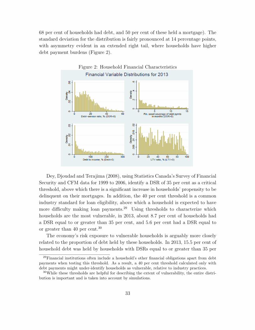
68 per cent of households had debt, and 50 per cent of these held a mortgage). The
standard deviation for the distribution is fairly pronounced at 14 percentage points,
with asymmetry evident in an extended right tail, where households have higher
debt payment burdens (Figure 2).
Figure 2: Household Financial Characteristics
Dey, Djoudad and Terajima (2008), using Statistics Canada’s Survey of Financial
Security and CFM data for 1999 to 2006, identify a DSR of 35 per cent as a critical
threshold, above which there is a significant increase in households’ propensity to be
delinquent on their mortgages. In addition, the 40 per cent threshold is a common
industry standard for loan eligibility, above which a household is expected to have
more difficulty making loan payments.29 Using thresholds to characterize which
households are the most vulnerable, in 2013, about 8.7 per cent of households had
a DSR equal to or greater than 35 per cent, and 5.6 per cent had a DSR equal to
or greater than 40 per cent.30
The economy’s risk exposure to vulnerable households is arguably more closely
related to the proportion of debt held by these households. In 2013, 15.5 per cent of
household debt was held by households with DSRs equal to or greater than 35 per
29Financial institutions often include a household’s other financial obligations apart from debtpayments when testing this threshold. As a result, a 40 per cent threshold calculated only withdebt payments might under-identify households as vulnerable, relative to industry practices.
30While these thresholds are helpful for describing the extent of vulnerability, the entire distri-bution is important and is taken into account by simulations.
33
cent, while this figure was 9.9 per cent for household debt held by households with
DSRs equal to or greater than 40 per cent.31
The debt-service burden is determined in part by interest rates, however, and
could understate vulnerabilities, given the current low interest rate environment. As
discussed in Cateau, Roberts, and Zhou (2015), the share of household debt held
by highly indebted households (which they define as having a debt-to-gross-income
ratio of 350 per cent and above) has increased from 12.7 per cent over 2005-2007
to 20.7 over 2012-2014. Cateau et al. provide a more comprehensive description of
these highly indebted households and possible implications for Canadian financial
system vulnerabilities from this increase.
Financial assets are also of particular interest, since these assets would be the
most readily available alternative as a buffer in the event of a temporary loss of in-
come. To put financial assets into perspective, we divide these holdings by a house-
hold’s reported monthly debt payment obligations to give the number of months
that a household could meet its debt obligations without recourse to any income
(either labour or non-labour income). The top-right quadrant of Figure 2 illustrates
that many indebted households have only enough financial assets to cover a couple
of months of payments. The chart is truncated at 15 months because of the ex-
tended right tail of households with high levels of financial assets relative to debt
payments.
To give a rough indication of the share of households that could have insuffi-
cient financial assets in the event of an income shock, threshold measures can help
to describe the tail of the distribution. One month and four months of coverage
are chosen as thresholds because the average complete unemployment episode lasts
about four months. Abstracting from minimum consumption requirements and any
alternative resources from which to make debt payments, one month of coverage
would bring a household just to the point of the three-month arrears threshold,
subject to an average unemployment episode; four months would bring a household
to the point of a total drawdown of financial assets. The overall proportions for
households that met or fell below these two thresholds in 2013 were 7.4 per cent and
15.8 per cent, respectively.32
31These measures describe the tail of the distribution and so are particularly affected by samplingvariability. In a given year, about 450 households might have a DSR ≥ 40 per cent (accounting formissing survey responses). Higher sampling weights for certain observations can potentially addto this variability. Bootstrapping the share of households with a DSR ≥ 40 for 2013 roughly gives5.6 per cent ± 0.5 percentage points at a 90 per cent confidence interval. For the share of debtheld by households with a DSR ≥ 40 per cent, the confidence interval is roughly 9.9 per cent ±1.1 percentage points, at a 90 per cent confidence interval.
32These measures should be interpreted as only being indicative. Estimates of minimum con-sumption requirements and any alternative sources of income, such as employment insurance, may
34
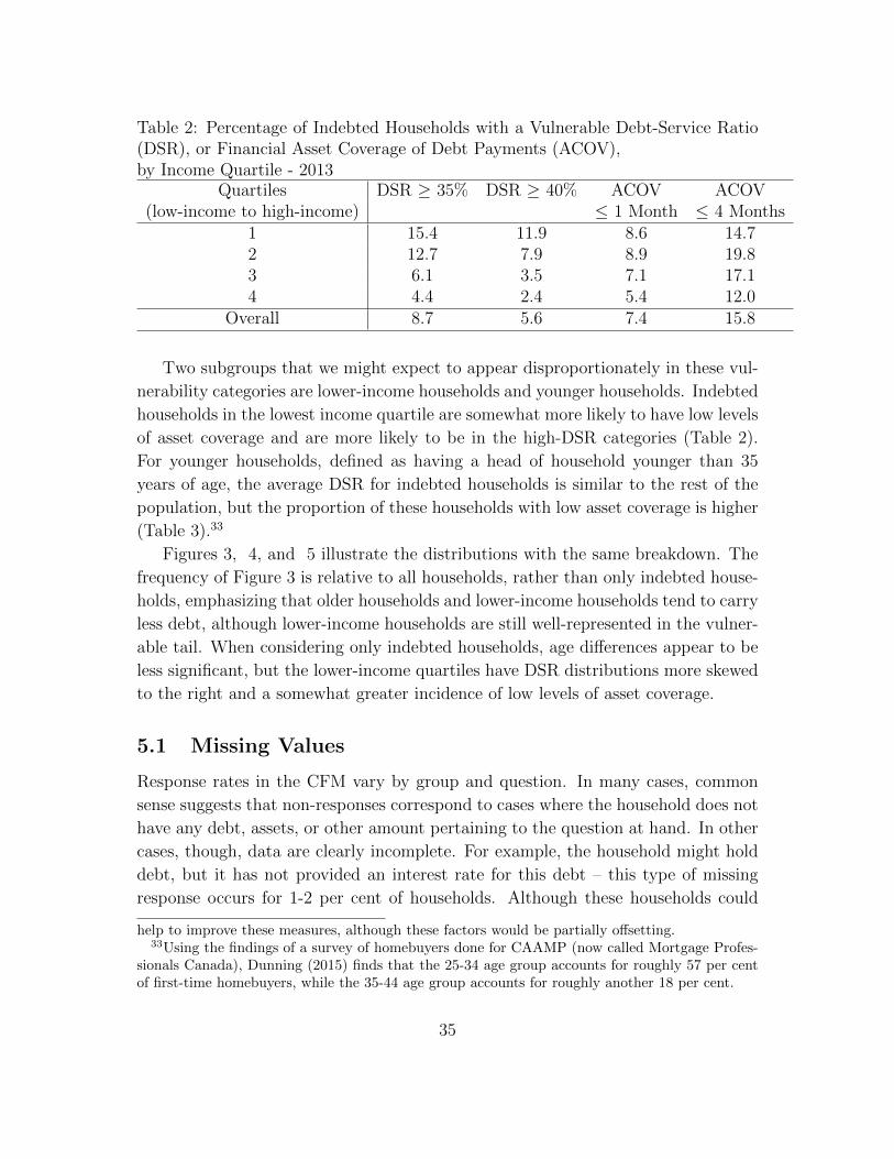
Table 2: Percentage of Indebted Households with a Vulnerable Debt-Service Ratio(DSR), or Financial Asset Coverage of Debt Payments (ACOV),by Income Quartile - 2013
Quartiles DSR ≥ 35% DSR ≥ 40% ACOV ACOV(low-income to high-income) ≤ 1 Month ≤ 4 Months
1 15.4 11.9 8.6 14.72 12.7 7.9 8.9 19.83 6.1 3.5 7.1 17.14 4.4 2.4 5.4 12.0
Overall 8.7 5.6 7.4 15.8
Two subgroups that we might expect to appear disproportionately in these vul-
nerability categories are lower-income households and younger households. Indebted
households in the lowest income quartile are somewhat more likely to have low levels
of asset coverage and are more likely to be in the high-DSR categories (Table 2).
For younger households, defined as having a head of household younger than 35
years of age, the average DSR for indebted households is similar to the rest of the
population, but the proportion of these households with low asset coverage is higher
(Table 3).33
Figures 3, 4, and 5 illustrate the distributions with the same breakdown. The
frequency of Figure 3 is relative to all households, rather than only indebted house-
holds, emphasizing that older households and lower-income households tend to carry
less debt, although lower-income households are still well-represented in the vulner-
able tail. When considering only indebted households, age differences appear to be
less significant, but the lower-income quartiles have DSR distributions more skewed
to the right and a somewhat greater incidence of low levels of asset coverage.
5.1 Missing Values
Response rates in the CFM vary by group and question. In many cases, common
sense suggests that non-responses correspond to cases where the household does not
have any debt, assets, or other amount pertaining to the question at hand. In other
cases, though, data are clearly incomplete. For example, the household might hold
debt, but it has not provided an interest rate for this debt – this type of missing
response occurs for 1-2 per cent of households. Although these households could
help to improve these measures, although these factors would be partially offsetting.33Using the findings of a survey of homebuyers done for CAAMP (now called Mortgage Profes-
sionals Canada), Dunning (2015) finds that the 25-34 age group accounts for roughly 57 per centof first-time homebuyers, while the 35-44 age group accounts for roughly another 18 per cent.
35
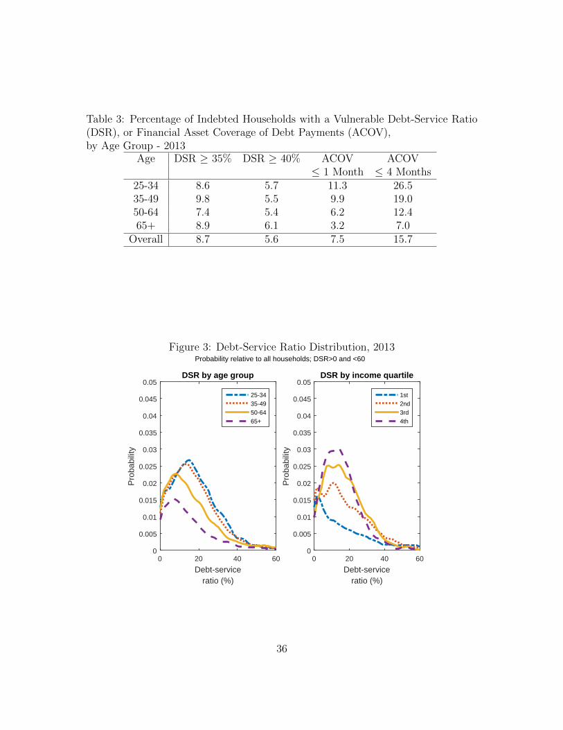
Table 3: Percentage of Indebted Households with a Vulnerable Debt-Service Ratio(DSR), or Financial Asset Coverage of Debt Payments (ACOV),by Age Group - 2013
Age DSR ≥ 35% DSR ≥ 40% ACOV ACOV≤ 1 Month ≤ 4 Months
25-34 8.6 5.7 11.3 26.535-49 9.8 5.5 9.9 19.050-64 7.4 5.4 6.2 12.465+ 8.9 6.1 3.2 7.0
Overall 8.7 5.6 7.5 15.7
Figure 3: Debt-Service Ratio Distribution, 2013
Debt-serviceratio (%)
0 20 40 60
Pro
babi
lity
0
0.005
0.01
0.015
0.02
0.025
0.03
0.035
0.04
0.045
0.05DSR by age group
25-3435-4950-6465+
Debt-serviceratio (%)
0 20 40 60
Pro
babi
lity
0
0.005
0.01
0.015
0.02
0.025
0.03
0.035
0.04
0.045
0.05DSR by income quartile
1st2nd3rd4th
Probability relative to all households; DSR>0 and <60
36
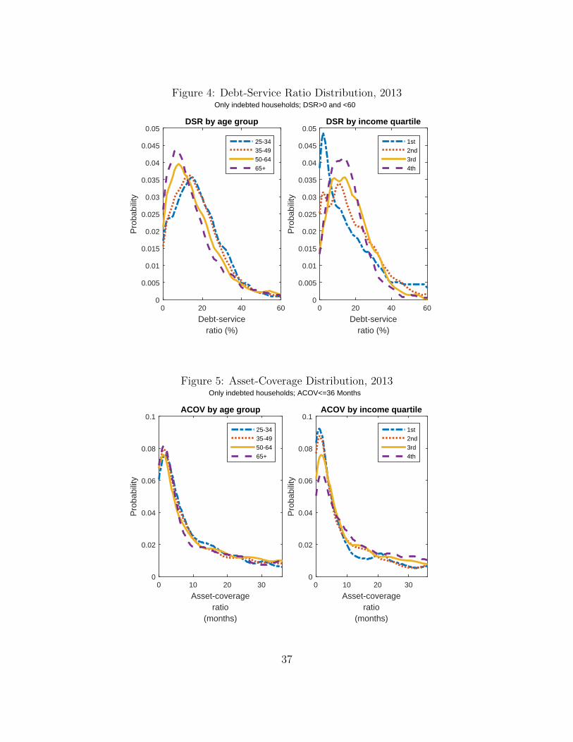
Figure 4: Debt-Service Ratio Distribution, 2013
Debt-serviceratio (%)
0 20 40 60
Pro
babi
lity
0
0.005
0.01
0.015
0.02
0.025
0.03
0.035
0.04
0.045
0.05DSR by age group
25-3435-4950-6465+
Debt-serviceratio (%)
0 20 40 60
Pro
babi
lity
0
0.005
0.01
0.015
0.02
0.025
0.03
0.035
0.04
0.045
0.05DSR by income quartile
1st2nd3rd4th
Only indebted households; DSR>0 and <60
Figure 5: Asset-Coverage Distribution, 2013
Asset-coverageratio
(months)
0 10 20 30
Pro
babi
lity
0
0.02
0.04
0.06
0.08
0.1ACOV by age group
25-3435-4950-6465+
Asset-coverageratio
(months)
0 10 20 30
Pro
babi
lity
0
0.02
0.04
0.06
0.08
0.1ACOV by income quartile
1st2nd3rd4th
Only indebted households; ACOV<=36 Months
37
simply be excluded, this presents the risk of biasing the sample (Djoudad 2012).
For missing interest rates and risk premiums, a household is assigned the average
value from households in its income group for that same loan type. For the mortgage
term and rate type (variable or fixed), a random draw is made from the existing
distribution of available responses. Missing balance amounts are not replaced –
related debt payments are assumed to stay unchanged over the simulation.
Other assumptions:
• All consumer debt, except for credit cards, is assumed to be at variable rates.
• For this consumer debt, households pay the overnight rate, plus an individual
premium calculated at the starting point. This individual premium stays
unchanged throughout the simulation, although a stress scenario could involve
an increase to the general household-sector premium.
• There is full pass-through of changes to the overnight rate and aggregate
changes to risk premiums, to all variable-rate debt, in each period. There
is pass-through to fixed-rate mortgages only at renewal.
• Variable-rate mortgages are renewed as either fixed or variable, in proportions
corresponding to current trends.34
• The CFM has information on the rate types and terms of mortgages, but does
not say when mortgages are due for renewal. Renewal is staggered across pe-
riods, so that households with a specific mortgage term renew their mortgages
evenly across simulation periods.
34The Bank of Canada’s Financial System Review periodically discusses trends in the residentialmortgage market. For instance, about 32 per cent of new mortgages in April 2015 had variablerates, a significant increase from about 9 per cent two years earlier. More than one-quarter of theoutstanding stock of mortgages were at variable rates (Bank of Canada, 2015).
38
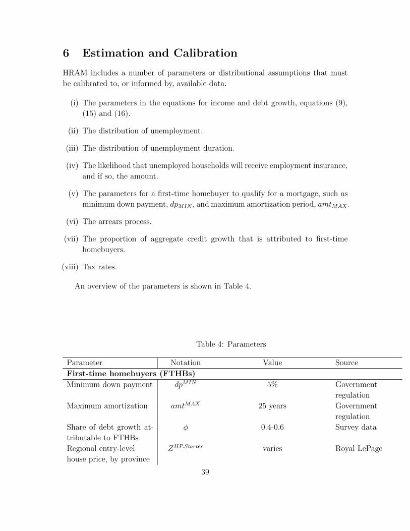
6 Estimation and Calibration
HRAM includes a number of parameters or distributional assumptions that must
be calibrated to, or informed by, available data:
(i) The parameters in the equations for income and debt growth, equations (9),
(15) and (16).
(ii) The distribution of unemployment.
(iii) The distribution of unemployment duration.
(iv) The likelihood that unemployed households will receive employment insurance,
and if so, the amount.
(v) The parameters for a first-time homebuyer to qualify for a mortgage, such as
minimum down payment, dpMIN , and maximum amortization period, amtMAX .
(vi) The arrears process.
(vii) The proportion of aggregate credit growth that is attributed to first-time
homebuyers.
(viii) Tax rates.
An overview of the parameters is shown in Table 4.
Table 4: Parameters
Parameter Notation Value Source
First-time homebuyers (FTHBs)
Minimum down payment dpMIN 5% Government
regulation
Maximum amortization amtMAX 25 years Government
regulation
Share of debt growth at-
tributable to FTHBs
φ 0.4-0.6 Survey data
Regional entry-level
house price, by province
ZHP.Starter varies Royal LePage
39
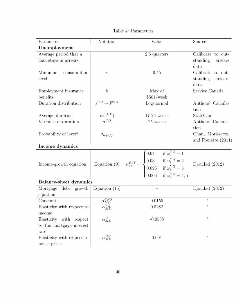
Table 4: Parameters
Parameter Notation Value Source
Unemployment
Average period that a
loan stays in arrears
2.5 quarters Calibrate to out-
standing arrears
data
Minimum consumption
level
κ 0.45 Calibrate to out-
standing arrears
data
Employment insurance
benefits
b Max of
$501/week
Service Canada
Duration distribution εUD ∼ FUD Log-normal Authors’ Calcula-
tion
Average duration E(εUD) 17-25 weeks StatsCan
Variance of duration σUD 25 weeks Authors’ Calcula-
tion
Probability of layoff βlayoff – Chan, Morissette,
and Frenette (2011)
Income dynamics
Income-growth equation Equation (9) σPLYi,t =
0.04 if ωY Qi = 1
0.03 if ωY Qi = 2
0.025 if ωY Qi = 3
0.006 if ωY Qi = 4, 5
Djoudad (2012)
Balance-sheet dynamics
Mortgage debt growth
equation
Equation (15) – Djoudad (2012)
Constant αCNSMD 0.0155 ''Elasticity with respect to
income
αY GMD 0.5282 ''
Elasticity with respect
to the mortgage interest
rate
αRMD -0.0538 ''
Elasticity with respect to
house prices
αHPMD 0.001 ''
40
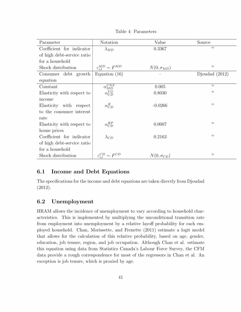
Table 4: Parameters
Parameter Notation Value Source
Coefficient for indicator
of high debt-service ratio
for a household
λMD 0.3367 ''
Shock distribution εMDi,t ∼ FMD N(0, σMD) ''
Consumer debt growth
equation
Equation (16) – Djoudad (2012)
Constant αCNSMD 0.005 ''Elasticity with respect to
income
αY GCD 0.8030 ''
Elasticity with respect
to the consumer interest
rate
αRCD -0.0266 ''
Elasticity with respect to
house prices
αHPCD 0.0007 ''
Coefficient for indicator
of high debt-service ratio
for a household
λCD 0.2163 ''
Shock distribution εCDi,t ∼ FCD N(0, σCD) ''
6.1 Income and Debt Equations
The specifications for the income and debt equations are taken directly from Djoudad
(2012).
6.2 Unemployment
HRAM allows the incidence of unemployment to vary according to household char-
acteristics. This is implemented by multiplying the unconditional transition rate
from employment into unemployment by a relative layoff probability for each em-
ployed household. Chan, Morissette, and Frenette (2011) estimate a logit model
that allows for the calculation of this relative probability, based on age, gender,
education, job tenure, region, and job occupation. Although Chan et al. estimate
this equation using data from Statistics Canada’s Labour Force Survey, the CFM
data provide a rough correspondence for most of the regressors in Chan et al. An
exception is job tenure, which is proxied by age.
41
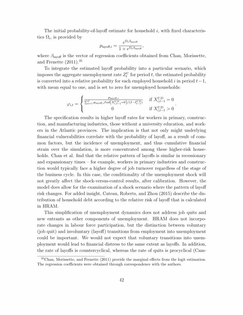
The initial probability-of-layoff estimate for household i, with fixed characteris-
tics Ωi, is provided by
playoff,i =eΩiβlayoff
1 + eΩiβlayoff,
where βlayoff is the vector of regression coefficients obtained from Chan, Morissette,
and Frenette (2011).35
To integrate the estimated layoff probability into a particular scenario, which
imposes the aggregate unemployment rate ZUt for period t, the estimated probability
is converted into a relative probability for each employed household i in period t−1,
with mean equal to one, and is set to zero for unemployed households:
ϕi,t =
playoff,i∑I
i=1 playoff,iInd(XUDi,t−1=0)/(I−IUD
t−1)if XUD
i,t−1 = 0
0 if XUDi,t−1 > 0
.
The specification results in higher layoff rates for workers in primary, construc-
tion, and manufacturing industries, those without a university education, and work-
ers in the Atlantic provinces. The implication is that not only might underlying
financial vulnerabilities correlate with the probability of layoff, as a result of com-
mon factors, but the incidence of unemployment, and thus cumulative financial
strain over the simulation, is more concentrated among these higher-risk house-
holds. Chan et al. find that the relative pattern of layoffs is similar in recessionary
and expansionary times – for example, workers in primary industries and construc-
tion would typically face a higher degree of job turnover regardless of the stage of
the business cycle. In this case, the conditionality of the unemployment shock will
not greatly affect the shock-versus-control results, after calibration. However, the
model does allow for the examination of a shock scenario where the pattern of layoff
risk changes. For added insight, Cateau, Roberts, and Zhou (2015) describe the dis-
tribution of household debt according to the relative risk of layoff that is calculated
in HRAM.
This simplification of unemployment dynamics does not address job quits and
new entrants as other components of unemployment. HRAM does not incorpo-
rate changes in labour force participation, but the distinction between voluntary
(job quit) and involuntary (layoff) transitions from employment into unemployment
could be important. We would not expect that voluntary transitions into unem-
ployment would lead to financial distress to the same extent as layoffs. In addition,
the rate of layoffs is countercyclical, whereas the rate of quits is procyclical (Cam-
35Chan, Morissette, and Frenette (2011) provide the marginal effects from the logit estimation.The regression coefficients were obtained through correspondence with the authors.
42
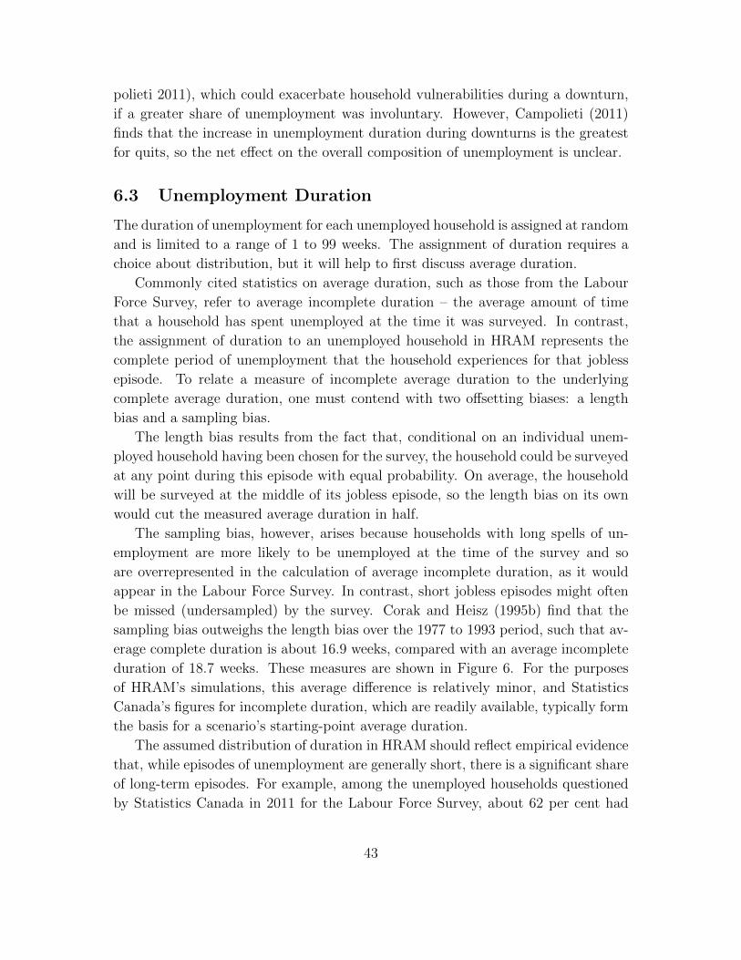
polieti 2011), which could exacerbate household vulnerabilities during a downturn,
if a greater share of unemployment was involuntary. However, Campolieti (2011)
finds that the increase in unemployment duration during downturns is the greatest
for quits, so the net effect on the overall composition of unemployment is unclear.
6.3 Unemployment Duration
The duration of unemployment for each unemployed household is assigned at random
and is limited to a range of 1 to 99 weeks. The assignment of duration requires a
choice about distribution, but it will help to first discuss average duration.
Commonly cited statistics on average duration, such as those from the Labour
Force Survey, refer to average incomplete duration – the average amount of time
that a household has spent unemployed at the time it was surveyed. In contrast,
the assignment of duration to an unemployed household in HRAM represents the
complete period of unemployment that the household experiences for that jobless
episode. To relate a measure of incomplete average duration to the underlying
complete average duration, one must contend with two offsetting biases: a length
bias and a sampling bias.
The length bias results from the fact that, conditional on an individual unem-
ployed household having been chosen for the survey, the household could be surveyed
at any point during this episode with equal probability. On average, the household
will be surveyed at the middle of its jobless episode, so the length bias on its own
would cut the measured average duration in half.
The sampling bias, however, arises because households with long spells of un-
employment are more likely to be unemployed at the time of the survey and so
are overrepresented in the calculation of average incomplete duration, as it would
appear in the Labour Force Survey. In contrast, short jobless episodes might often
be missed (undersampled) by the survey. Corak and Heisz (1995b) find that the
sampling bias outweighs the length bias over the 1977 to 1993 period, such that av-
erage complete duration is about 16.9 weeks, compared with an average incomplete
duration of 18.7 weeks. These measures are shown in Figure 6. For the purposes
of HRAM’s simulations, this average difference is relatively minor, and Statistics
Canada’s figures for incomplete duration, which are readily available, typically form
the basis for a scenario’s starting-point average duration.
The assumed distribution of duration in HRAM should reflect empirical evidence
that, while episodes of unemployment are generally short, there is a significant share
of long-term episodes. For example, among the unemployed households questioned
by Statistics Canada in 2011 for the Labour Force Survey, about 62 per cent had
43
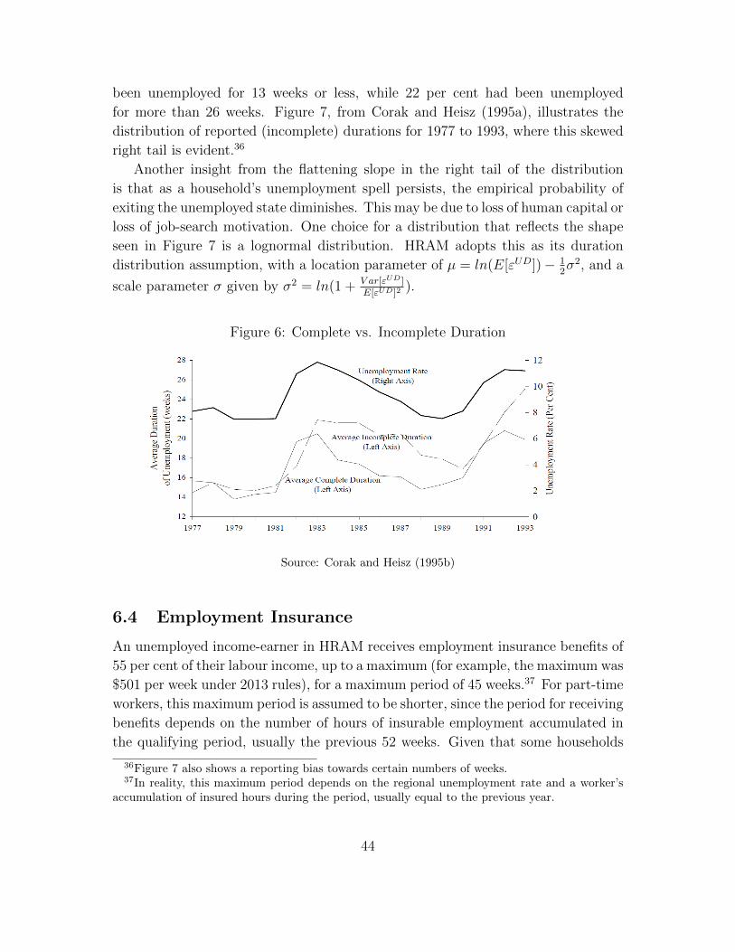
been unemployed for 13 weeks or less, while 22 per cent had been unemployed
for more than 26 weeks. Figure 7, from Corak and Heisz (1995a), illustrates the
distribution of reported (incomplete) durations for 1977 to 1993, where this skewed
right tail is evident.36
Another insight from the flattening slope in the right tail of the distribution
is that as a household’s unemployment spell persists, the empirical probability of
exiting the unemployed state diminishes. This may be due to loss of human capital or
loss of job-search motivation. One choice for a distribution that reflects the shape
seen in Figure 7 is a lognormal distribution. HRAM adopts this as its duration
distribution assumption, with a location parameter of µ = ln(E[εUD])− 12σ2, and a
scale parameter σ given by σ2 = ln(1 + V ar[εUD]E[εUD]2
).
Figure 6: Complete vs. Incomplete Duration
Source: Corak and Heisz (1995b)
6.4 Employment Insurance
An unemployed income-earner in HRAM receives employment insurance benefits of
55 per cent of their labour income, up to a maximum (for example, the maximum was
$501 per week under 2013 rules), for a maximum period of 45 weeks.37 For part-time
workers, this maximum period is assumed to be shorter, since the period for receiving
benefits depends on the number of hours of insurable employment accumulated in
the qualifying period, usually the previous 52 weeks. Given that some households
36Figure 7 also shows a reporting bias towards certain numbers of weeks.37In reality, this maximum period depends on the regional unemployment rate and a worker’s
accumulation of insured hours during the period, usually equal to the previous year.
44
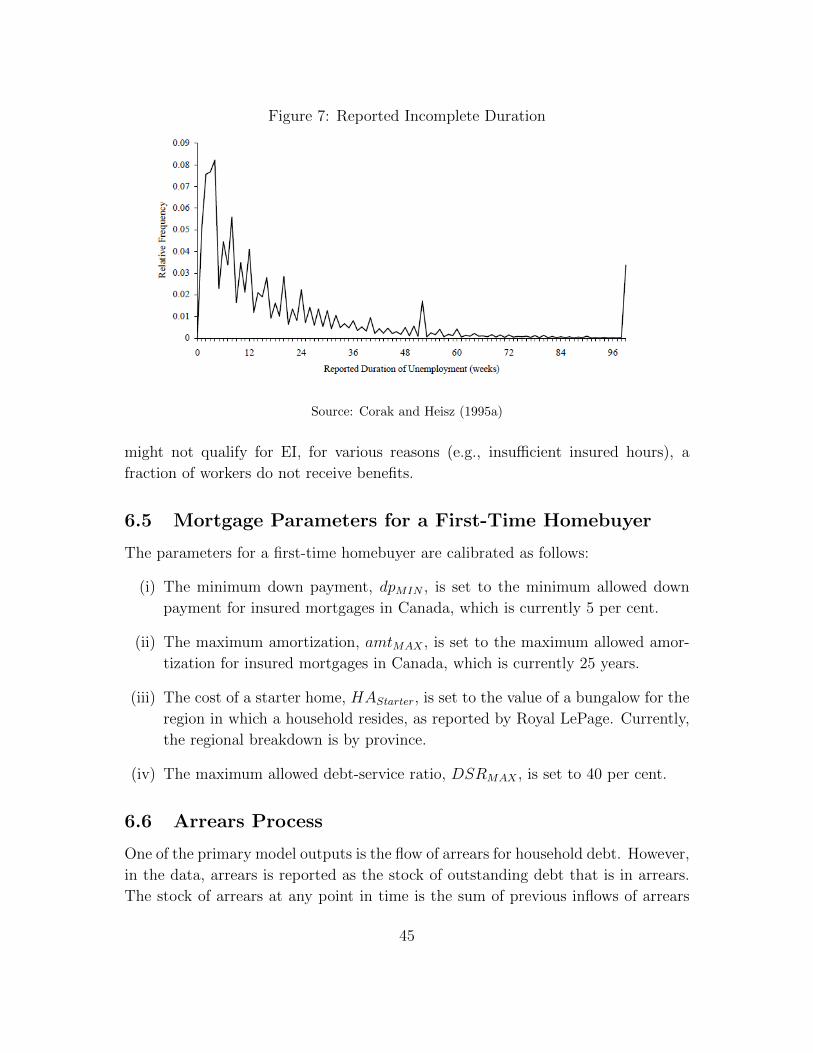
Figure 7: Reported Incomplete Duration
Source: Corak and Heisz (1995a)
might not qualify for EI, for various reasons (e.g., insufficient insured hours), a
fraction of workers do not receive benefits.
6.5 Mortgage Parameters for a First-Time Homebuyer
The parameters for a first-time homebuyer are calibrated as follows:
(i) The minimum down payment, dpMIN , is set to the minimum allowed down
payment for insured mortgages in Canada, which is currently 5 per cent.
(ii) The maximum amortization, amtMAX , is set to the maximum allowed amor-
tization for insured mortgages in Canada, which is currently 25 years.
(iii) The cost of a starter home, HAStarter, is set to the value of a bungalow for the
region in which a household resides, as reported by Royal LePage. Currently,
the regional breakdown is by province.
(iv) The maximum allowed debt-service ratio, DSRMAX , is set to 40 per cent.
6.6 Arrears Process
One of the primary model outputs is the flow of arrears for household debt. However,
in the data, arrears is reported as the stock of outstanding debt that is in arrears.
The stock of arrears at any point in time is the sum of previous inflows of arrears
45
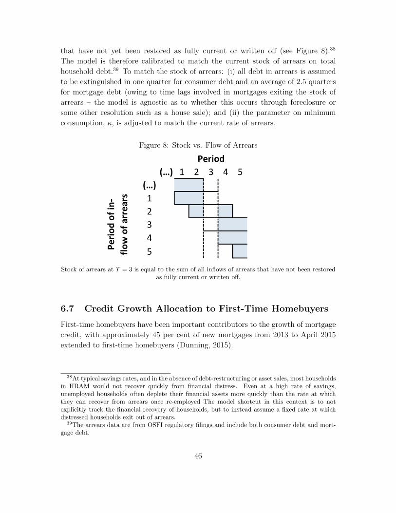
that have not yet been restored as fully current or written off (see Figure 8).38
The model is therefore calibrated to match the current stock of arrears on total
household debt.39 To match the stock of arrears: (i) all debt in arrears is assumed
to be extinguished in one quarter for consumer debt and an average of 2.5 quarters
for mortgage debt (owing to time lags involved in mortgages exiting the stock of
arrears – the model is agnostic as to whether this occurs through foreclosure or
some other resolution such as a house sale); and (ii) the parameter on minimum
consumption, κ, is adjusted to match the current rate of arrears.
Figure 8: Stock vs. Flow of Arrears
(…) 1 2 3 4 5(…)12345
Period
Perio
d of
in-
flow
of a
rrea
rs
Stock of arrears at T = 3 is equal to the sum of all inflows of arrears that have not been restoredas fully current or written off.
6.7 Credit Growth Allocation to First-Time Homebuyers
First-time homebuyers have been important contributors to the growth of mortgage
credit, with approximately 45 per cent of new mortgages from 2013 to April 2015
extended to first-time homebuyers (Dunning, 2015).
38At typical savings rates, and in the absence of debt-restructuring or asset sales, most householdsin HRAM would not recover quickly from financial distress. Even at a high rate of savings,unemployed households often deplete their financial assets more quickly than the rate at whichthey can recover from arrears once re-employed The model shortcut in this context is to notexplicitly track the financial recovery of households, but to instead assume a fixed rate at whichdistressed households exit out of arrears.
39The arrears data are from OSFI regulatory filings and include both consumer debt and mort-gage debt.
46
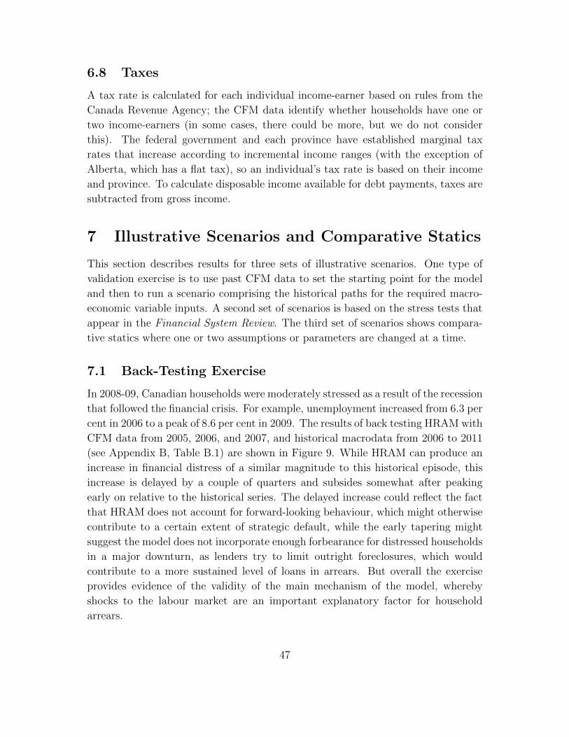
6.8 Taxes
A tax rate is calculated for each individual income-earner based on rules from the
Canada Revenue Agency; the CFM data identify whether households have one or
two income-earners (in some cases, there could be more, but we do not consider
this). The federal government and each province have established marginal tax
rates that increase according to incremental income ranges (with the exception of
Alberta, which has a flat tax), so an individual’s tax rate is based on their income
and province. To calculate disposable income available for debt payments, taxes are
subtracted from gross income.
7 Illustrative Scenarios and Comparative Statics
This section describes results for three sets of illustrative scenarios. One type of
validation exercise is to use past CFM data to set the starting point for the model
and then to run a scenario comprising the historical paths for the required macro-
economic variable inputs. A second set of scenarios is based on the stress tests that
appear in the Financial System Review. The third set of scenarios shows compara-
tive statics where one or two assumptions or parameters are changed at a time.
7.1 Back-Testing Exercise
In 2008-09, Canadian households were moderately stressed as a result of the recession
that followed the financial crisis. For example, unemployment increased from 6.3 per
cent in 2006 to a peak of 8.6 per cent in 2009. The results of back testing HRAM with
CFM data from 2005, 2006, and 2007, and historical macrodata from 2006 to 2011
(see Appendix B, Table B.1) are shown in Figure 9. While HRAM can produce an
increase in financial distress of a similar magnitude to this historical episode, this
increase is delayed by a couple of quarters and subsides somewhat after peaking
early on relative to the historical series. The delayed increase could reflect the fact
that HRAM does not account for forward-looking behaviour, which might otherwise
contribute to a certain extent of strategic default, while the early tapering might
suggest the model does not incorporate enough forbearance for distressed households
in a major downturn, as lenders try to limit outright foreclosures, which would
contribute to a more sustained level of loans in arrears. But overall the exercise
provides evidence of the validity of the main mechanism of the model, whereby
shocks to the labour market are an important explanatory factor for household
arrears.
47
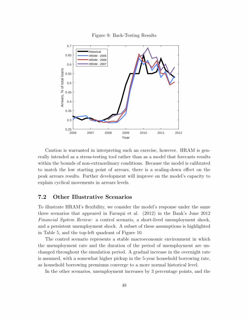
Figure 9: Back-Testing Results
Year2006 2007 2008 2009 2010 2011 2012
Arr
ears
, % o
f tot
al lo
ans
0.25
0.3
0.35
0.4
0.45
0.5
0.55
0.6
0.65
0.7
HistoricalHRAM - 2005HRAM - 2006HRAM - 2007
Caution is warranted in interpreting such an exercise, however. HRAM is gen-
erally intended as a stress-testing tool rather than as a model that forecasts results
within the bounds of non-extraordinary conditions. Because the model is calibrated
to match the low starting point of arrears, there is a scaling-down effect on the
peak arrears results. Further development will improve on the model’s capacity to
explain cyclical movements in arrears levels.
7.2 Other Illustrative Scenarios
To illustrate HRAM’s flexibility, we consider the model’s response under the same
three scenarios that appeared in Faruqui et al. (2012) in the Bank’s June 2012
Financial System Review : a control scenario, a short-lived unemployment shock,
and a persistent unemployment shock. A subset of these assumptions is highlighted
in Table 5, and the top-left quadrant of Figure 10.
The control scenario represents a stable macroeconomic environment in which
the unemployment rate and the duration of the period of unemployment are un-
changed throughout the simulation period. A gradual increase in the overnight rate
is assumed, with a somewhat higher pickup in the 5-year household borrowing rate,
as household borrowing premiums converge to a more normal historical level.
In the other scenarios, unemployment increases by 3 percentage points, and the
48
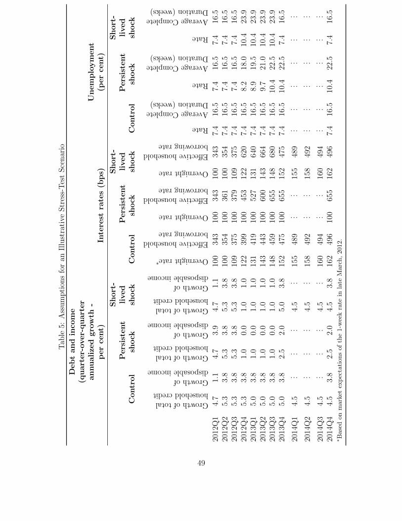
Tab
le5:
Ass
um
pti
ons
for
anIl
lust
rati
veStr
ess-
Tes
tSce
nar
io
Deb
tan
din
com
e(q
uart
er-
over-
quart
er
annualize
dgro
wth
-p
er
cent)
Inte
rest
rate
s(b
ps)
Unem
plo
ym
ent
(per
cent)
Contr
ol
Pers
iste
nt
shock
Short
-li
ved
shock
Contr
ol
Pers
iste
nt
shock
Short
-li
ved
shock
Contr
ol
Pers
iste
nt
shock
Short
-li
ved
shock
Growthoftotalhouseholdcredit
Growthofdisposableincome
Growthoftotalhouseholdcredit
Growthofdisposableincome
Growthoftotalhouseholdcredit
Growthofdisposableincome
Overnightrate∗
Effectivehouseholdborrowingrate
Overnightrate
Effectivehouseholdborrowingrate
Overnightrate
Effectivehouseholdborrowingrate
Rate
AverageCompleteDuration(weeks)
Rate
AverageCompleteDuration(weeks)
Rate
AverageCompleteDuration(weeks)
2012
Q1
4.7
1.1
4.7
3.9
4.7
1.1
100
343
100
343
100
343
7.4
16.5
7.4
16.5
7.4
16.5
2012
Q2
5.3
3.8
5.3
3.8
5.3
3.8
100
354
100
361
100
354
7.4
16.5
7.4
16.5
7.4
16.5
2012
Q3
5.3
3.8
5.3
3.8
5.3
3.8
109
375
100
379
109
375
7.4
16.5
7.4
16.5
7.4
16.5
2012
Q4
5.3
3.8
1.0
0.0
1.0
1.0
122
399
100
453
122
620
7.4
16.5
8.2
18.0
10.4
23.9
2013
Q1
5.0
3.8
1.0
0.0
1.0
1.0
131
419
100
527
131
640
7.4
16.5
8.9
19.5
10.4
23.9
2013
Q2
5.0
3.8
1.0
0.0
1.0
1.0
143
443
100
600
143
664
7.4
16.5
9.7
21.0
10.4
23.9
2013
Q3
5.0
3.8
1.0
0.0
1.0
1.0
148
459
100
655
148
680
7.4
16.5
10.4
22.5
10.4
23.9
2013
Q4
5.0
3.8
2.5
2.0
5.0
3.8
152
475
100
655
152
475
7.4
16.5
10.4
22.5
7.4
16.5
2014
Q1
4.5
. . .. . .
. . .4.
5. . .
155
489
. . .. . .
155
489
. . .. . .
. . .. . .
. . .. . .
2014
Q2
4.5
. . .. . .
. . .4.
5. . .
158
492
. . .. . .
158
492
. . .. . .
. . .. . .
. . .. . .
2014
Q3
4.5
. . .. . .
. . .4.
5. . .
160
494
. . .. . .
160
494
. . .. . .
. . .. . .
. . .. . .
2014
Q4
4.5
3.8
2.5
2.0
4.5
3.8
162
496
100
655
162
496
7.4
16.5
10.4
22.5
7.4
16.5
∗ Bas
edon
mar
ket
exp
ecta
tion
sof
the
1-w
eek
rate
inla
teM
arc
h,
2012.
49
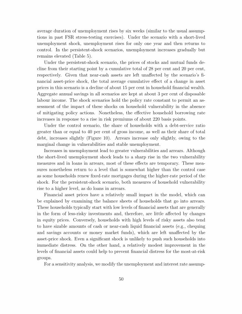
average duration of unemployment rises by six weeks (similar to the usual assump-
tions in past FSR stress-testing exercises). Under the scenario with a short-lived
unemployment shock, unemployment rises for only one year and then returns to
control. In the persistent-shock scenarios, unemployment increases gradually but
remains elevated (Table 5).
Under the persistent-shock scenario, the prices of stocks and mutual funds de-
cline from their starting point by a cumulative total of 28 per cent and 20 per cent,
respectively. Given that near-cash assets are left unaffected by the scenario’s fi-
nancial asset-price shock, the total average cumulative effect of a change in asset
prices in this scenario is a decline of about 15 per cent in household financial wealth.
Aggregate annual savings in all scenarios are kept at about 3 per cent of disposable
labour income. The shock scenarios hold the policy rate constant to permit an as-
sessment of the impact of these shocks on household vulnerability in the absence
of mitigating policy actions. Nonetheless, the effective household borrowing rate
increases in response to a rise in risk premiums of about 220 basis points.
Under the control scenario, the share of households with a debt-service ratio
greater than or equal to 40 per cent of gross income, as well as their share of total
debt, increases slightly (Figure 10). Arrears increase only slightly, owing to the
marginal change in vulnerabilities and stable unemployment.
Increases in unemployment lead to greater vulnerabilities and arrears. Although
the short-lived unemployment shock leads to a sharp rise in the two vulnerability
measures and in loans in arrears, most of these effects are temporary. These mea-
sures nonetheless return to a level that is somewhat higher than the control case
as some households renew fixed-rate mortgages during the higher-rate period of the
shock. For the persistent-shock scenario, both measures of household vulnerability
rise to a higher level, as do loans in arrears.
Financial asset prices have a relatively small impact in the model, which can
be explained by examining the balance sheets of households that go into arrears.
These households typically start with low levels of financial assets that are generally
in the form of less-risky investments and, therefore, are little affected by changes
in equity prices. Conversely, households with high levels of risky assets also tend
to have sizable amounts of cash or near-cash liquid financial assets (e.g., chequing
and savings accounts or money market funds), which are left unaffected by the
asset-price shock. Even a significant shock is unlikely to push such households into
immediate distress. On the other hand, a relatively modest improvement in the
levels of financial assets could help to prevent financial distress for the most-at-risk
groups.
For a sensitivity analysis, we modify the unemployment and interest rate assump-
50
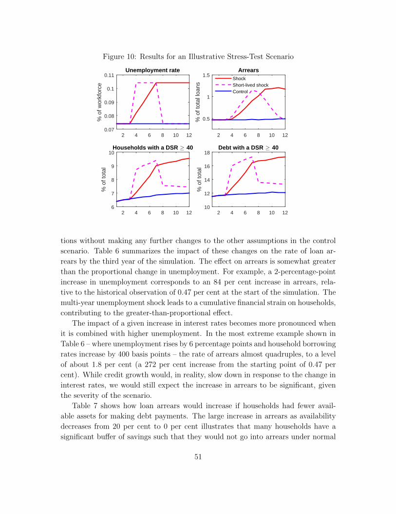
Figure 10: Results for an Illustrative Stress-Test Scenario
2 4 6 8 10 12
% o
f wor
kfor
ce
0.07
0.08
0.09
0.1
0.11Unemployment rate
2 4 6 8 10 12
% o
f tot
al lo
ans
0.5
1
1.5Arrears
ShockShort-lived shockControl
2 4 6 8 10 12
% o
f tot
al
6
7
8
9
10Households with a DSR ≥ 40
2 4 6 8 10 12
% o
f tot
al10
12
14
16
18Debt with a DSR ≥ 40
tions without making any further changes to the other assumptions in the control
scenario. Table 6 summarizes the impact of these changes on the rate of loan ar-
rears by the third year of the simulation. The effect on arrears is somewhat greater
than the proportional change in unemployment. For example, a 2-percentage-point
increase in unemployment corresponds to an 84 per cent increase in arrears, rela-
tive to the historical observation of 0.47 per cent at the start of the simulation. The
multi-year unemployment shock leads to a cumulative financial strain on households,
contributing to the greater-than-proportional effect.
The impact of a given increase in interest rates becomes more pronounced when
it is combined with higher unemployment. In the most extreme example shown in
Table 6 – where unemployment rises by 6 percentage points and household borrowing
rates increase by 400 basis points – the rate of arrears almost quadruples, to a level
of about 1.8 per cent (a 272 per cent increase from the starting point of 0.47 per
cent). While credit growth would, in reality, slow down in response to the change in
interest rates, we would still expect the increase in arrears to be significant, given
the severity of the scenario.
Table 7 shows how loan arrears would increase if households had fewer avail-
able assets for making debt payments. The large increase in arrears as availability
decreases from 20 per cent to 0 per cent illustrates that many households have a
significant buffer of savings such that they would not go into arrears under normal
51
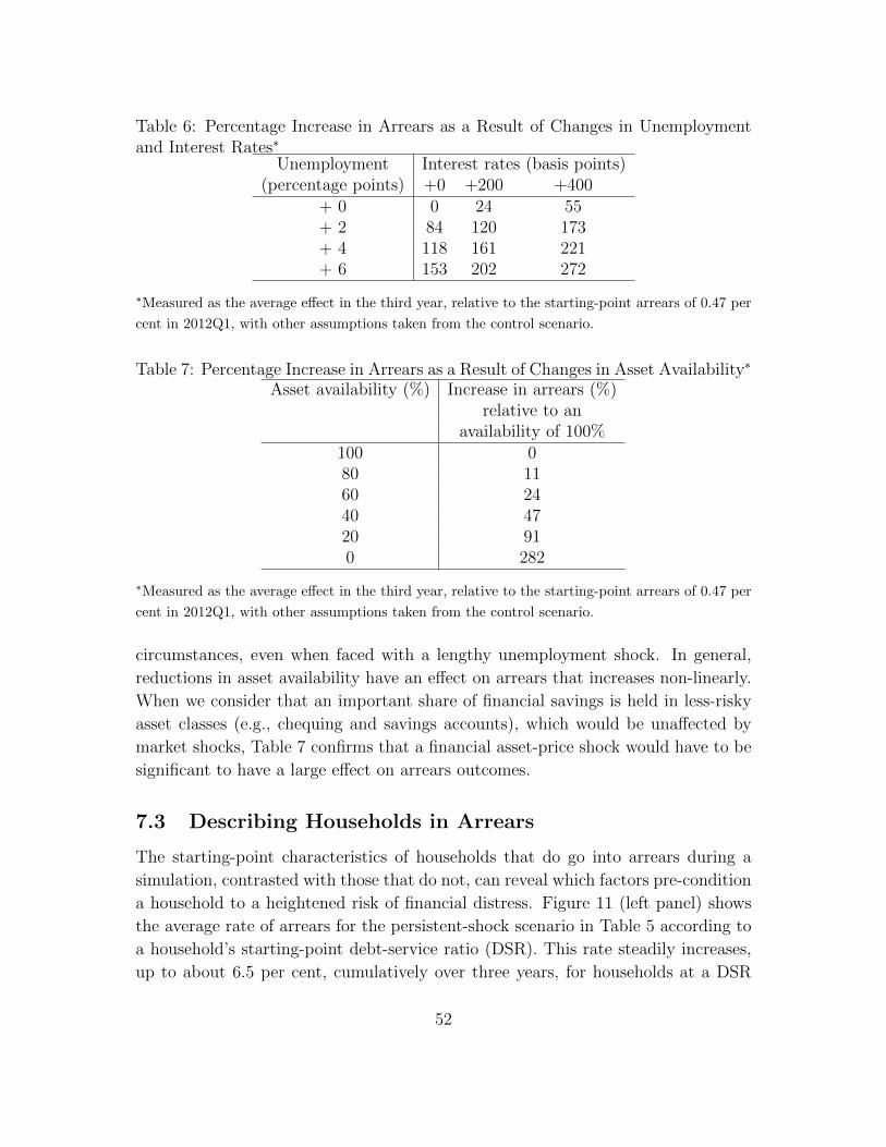
Table 6: Percentage Increase in Arrears as a Result of Changes in Unemploymentand Interest Rates∗
Unemployment Interest rates (basis points)(percentage points) +0 +200 +400
+ 0 0 24 55+ 2 84 120 173+ 4 118 161 221+ 6 153 202 272
∗Measured as the average effect in the third year, relative to the starting-point arrears of 0.47 per
cent in 2012Q1, with other assumptions taken from the control scenario.
Table 7: Percentage Increase in Arrears as a Result of Changes in Asset Availability∗
Asset availability (%) Increase in arrears (%)relative to an
availability of 100%100 080 1160 2440 4720 910 282
∗Measured as the average effect in the third year, relative to the starting-point arrears of 0.47 per
cent in 2012Q1, with other assumptions taken from the control scenario.
circumstances, even when faced with a lengthy unemployment shock. In general,
reductions in asset availability have an effect on arrears that increases non-linearly.
When we consider that an important share of financial savings is held in less-risky
asset classes (e.g., chequing and savings accounts), which would be unaffected by
market shocks, Table 7 confirms that a financial asset-price shock would have to be
significant to have a large effect on arrears outcomes.
7.3 Describing Households in Arrears
The starting-point characteristics of households that do go into arrears during a
simulation, contrasted with those that do not, can reveal which factors pre-condition
a household to a heightened risk of financial distress. Figure 11 (left panel) shows
the average rate of arrears for the persistent-shock scenario in Table 5 according to
a household’s starting-point debt-service ratio (DSR). This rate steadily increases,
up to about 6.5 per cent, cumulatively over three years, for households at a DSR
52
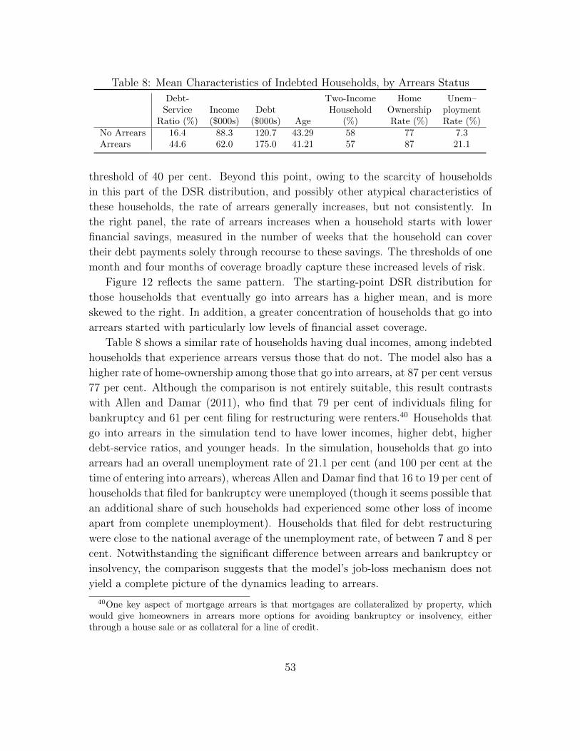
Table 8: Mean Characteristics of Indebted Households, by Arrears Status
Debt- Two-Income Home Unem–Service Income Debt Household Ownership ployment
Ratio (%) ($000s) ($000s) Age (%) Rate (%) Rate (%)No Arrears 16.4 88.3 120.7 43.29 58 77 7.3Arrears 44.6 62.0 175.0 41.21 57 87 21.1
threshold of 40 per cent. Beyond this point, owing to the scarcity of households
in this part of the DSR distribution, and possibly other atypical characteristics of
these households, the rate of arrears generally increases, but not consistently. In
the right panel, the rate of arrears increases when a household starts with lower
financial savings, measured in the number of weeks that the household can cover
their debt payments solely through recourse to these savings. The thresholds of one
month and four months of coverage broadly capture these increased levels of risk.
Figure 12 reflects the same pattern. The starting-point DSR distribution for
those households that eventually go into arrears has a higher mean, and is more
skewed to the right. In addition, a greater concentration of households that go into
arrears started with particularly low levels of financial asset coverage.
Table 8 shows a similar rate of households having dual incomes, among indebted
households that experience arrears versus those that do not. The model also has a
higher rate of home-ownership among those that go into arrears, at 87 per cent versus
77 per cent. Although the comparison is not entirely suitable, this result contrasts
with Allen and Damar (2011), who find that 79 per cent of individuals filing for
bankruptcy and 61 per cent filing for restructuring were renters.40 Households that
go into arrears in the simulation tend to have lower incomes, higher debt, higher
debt-service ratios, and younger heads. In the simulation, households that go into
arrears had an overall unemployment rate of 21.1 per cent (and 100 per cent at the
time of entering into arrears), whereas Allen and Damar find that 16 to 19 per cent of
households that filed for bankruptcy were unemployed (though it seems possible that
an additional share of such households had experienced some other loss of income
apart from complete unemployment). Households that filed for debt restructuring
were close to the national average of the unemployment rate, of between 7 and 8 per
cent. Notwithstanding the significant difference between arrears and bankruptcy or
insolvency, the comparison suggests that the model’s job-loss mechanism does not
yield a complete picture of the dynamics leading to arrears.
40One key aspect of mortgage arrears is that mortgages are collateralized by property, whichwould give homeowners in arrears more options for avoiding bankruptcy or insolvency, eitherthrough a house sale or as collateral for a line of credit.
53
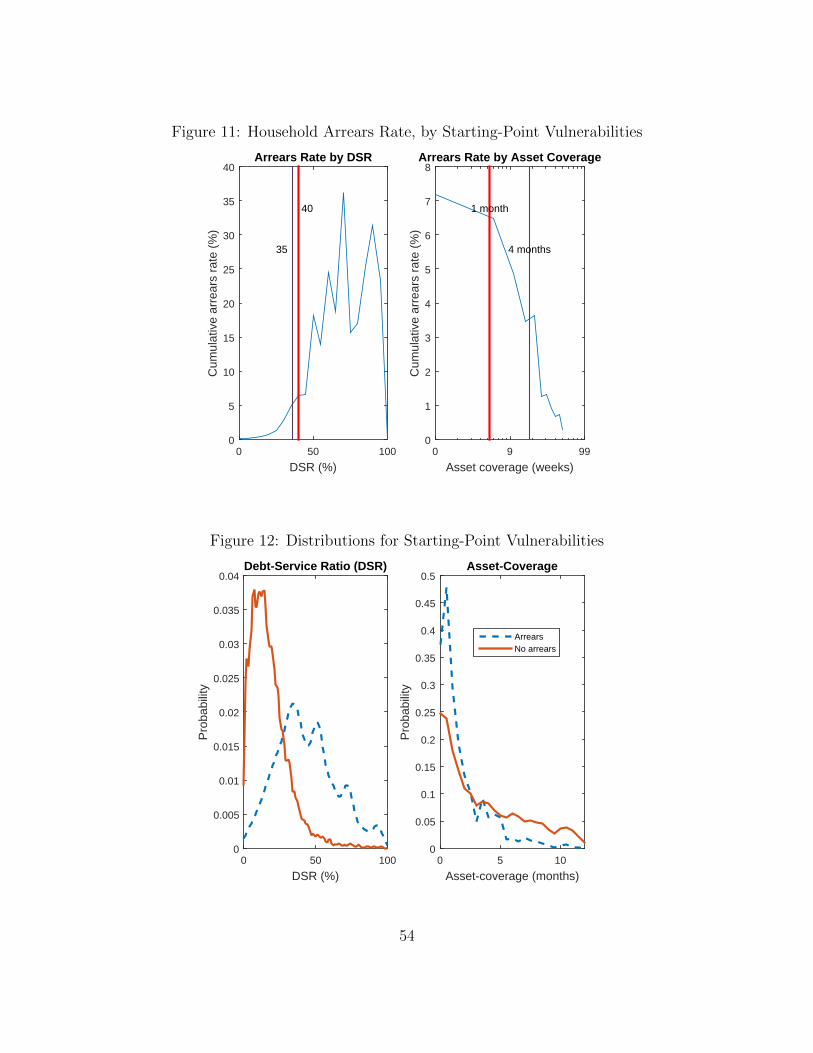
Figure 11: Household Arrears Rate, by Starting-Point Vulnerabilities
DSR (%)0 50 100
Cum
ulat
ive
arre
ars
rate
(%
)
0
5
10
15
20
25
30
35
40
40
35
Arrears Rate by DSR
Asset coverage (weeks)0 9 99
Cum
ulat
ive
arre
ars
rate
(%
)
0
1
2
3
4
5
6
7
8
1 month
4 months
Arrears Rate by Asset Coverage
Figure 12: Distributions for Starting-Point Vulnerabilities
DSR (%)0 50 100
Pro
babi
lity
0
0.005
0.01
0.015
0.02
0.025
0.03
0.035
0.04Debt-Service Ratio (DSR)
Asset-coverage (months)0 5 10
Pro
babi
lity
0
0.05
0.1
0.15
0.2
0.25
0.3
0.35
0.4
0.45
0.5Asset-Coverage
ArrearsNo arrears
54
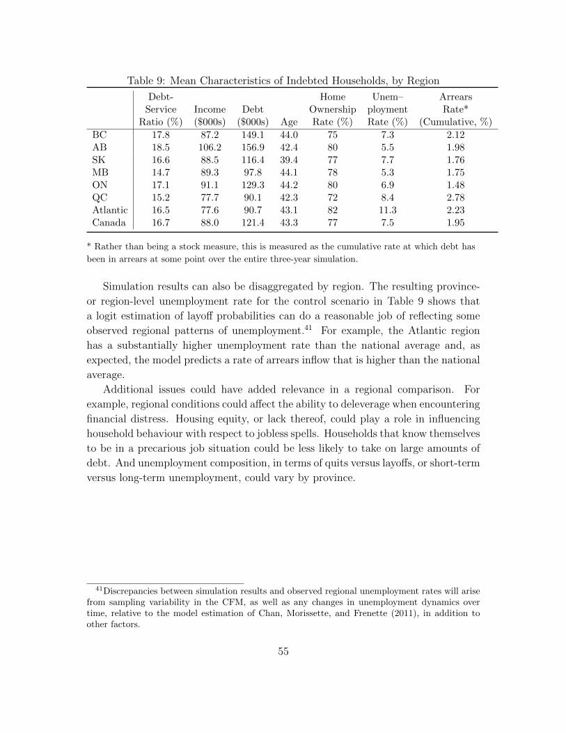
Table 9: Mean Characteristics of Indebted Households, by Region
Debt- Home Unem– ArrearsService Income Debt Ownership ployment Rate*
Ratio (%) ($000s) ($000s) Age Rate (%) Rate (%) (Cumulative, %)
BC 17.8 87.2 149.1 44.0 75 7.3 2.12AB 18.5 106.2 156.9 42.4 80 5.5 1.98SK 16.6 88.5 116.4 39.4 77 7.7 1.76MB 14.7 89.3 97.8 44.1 78 5.3 1.75ON 17.1 91.1 129.3 44.2 80 6.9 1.48QC 15.2 77.7 90.1 42.3 72 8.4 2.78Atlantic 16.5 77.6 90.7 43.1 82 11.3 2.23Canada 16.7 88.0 121.4 43.3 77 7.5 1.95
* Rather than being a stock measure, this is measured as the cumulative rate at which debt has
been in arrears at some point over the entire three-year simulation.
Simulation results can also be disaggregated by region. The resulting province-
or region-level unemployment rate for the control scenario in Table 9 shows that
a logit estimation of layoff probabilities can do a reasonable job of reflecting some
observed regional patterns of unemployment.41 For example, the Atlantic region
has a substantially higher unemployment rate than the national average and, as
expected, the model predicts a rate of arrears inflow that is higher than the national
average.
Additional issues could have added relevance in a regional comparison. For
example, regional conditions could affect the ability to deleverage when encountering
financial distress. Housing equity, or lack thereof, could play a role in influencing
household behaviour with respect to jobless spells. Households that know themselves
to be in a precarious job situation could be less likely to take on large amounts of
debt. And unemployment composition, in terms of quits versus layoffs, or short-term
versus long-term unemployment, could vary by province.
41Discrepancies between simulation results and observed regional unemployment rates will arisefrom sampling variability in the CFM, as well as any changes in unemployment dynamics overtime, relative to the model estimation of Chan, Morissette, and Frenette (2011), in addition toother factors.
55
8 Conclusions
Stress tests using microdata are a significant component in the assessment of the fi-
nancial stability risk related to household balance sheets. While aggregate measures
can describe important sectoral trends, it is at the micro level that we can better
assess the potential change in loan arrears under an adverse-shock scenario.
Further work is planned to strengthen HRAM’s empirical foundation. The mod-
elling of household-specific income and credit growth will be refined to better account
for the empirical determinants of these dynamics. In addition, the behavioural de-
tail in the model could be extended further. For example, the simulation does not
currently allow distressed households to sell their houses. If they are allowed to
do so, they can potentially avoid default, leading to lower arrears. This extension
would need to consider how the feasibility of this option would change in a severe
housing-market downturn with slower market turnover and falling house prices.
56
References
Aiyagari, R. (1994): “Uninsured Idiosyncratic Risk and Aggregate Saving,” Quar-
terly Journal of Economics, 103(6), 659–984.
Allen, J., and E. Damar (2011-2012): “Household Insolvency in Canada,” Bank
of Canada Review (Winter): 43–54.
Bank of Canada (2015): “Assessment of Vulnerabilities and Risks,” Financial
System Review (June).
Bernanke, B., and M. Gertler (1989): “Agency Costs, Net Worth, and Busi-
ness Fluctuations,” American Economic Review, 79(1), 14–31.
Campolieti, M. (2011): “The ins and outs of unemployment in Canada, 1976-
2008,” Statistics Canada, 44(4).
Cateau, G., T. Roberts, and J. Zhou (2015): “Indebted Households and Po-
tential Vulnerabilities for the Canadian Financial System: A Microdata Analysis,”
Bank of Canada Financial System Review (December): 49–58.
Chan, W., R. Morissette, and M. Frenette (2011): “Workers Laid-off Dur-
ing the Last Three Recessions: Who Were They, and How Did They Fare?”
Statistics Canada (337).
Corak, M., and A. Heisz (1995a): “Alternative Measures of the Average Dura-
tion of Unemployment,” Statistics Canada (83).
(1995b): “The Duration of Unemployment: A User Guide,” Statistics
Canada (84).
Dey, S., R. Djoudad, and Y. Terajima (2008): “A Tool for Assessing the Fi-
nancial Vulnerabilities in the Household Sector,” Bank of Canada Review (Sum-
mer): 45–54.
Djoudad, R. (2012): “The Bank of Canada’s Analytic Framework for Assessing
the Vulnerability of the Household Sector,” Bank of Canada Discussion Paper
No. 2012-3.
Dunning, W. (2015): “A Profile of Home Buying in Canada,” Canadian Associa-
tion of Accredited Mortgage Professionals.
57
Faruqui, U., X. Liu, and T. Roberts (2012): “An Improved Framework for
Assessing the Risks Arising from Elevated Household Debt,” Bank of Canada
Financial System Review (June): 51–57.
Fuenzalida, M., and J. Ruiz-Tagle (2010): “Household Financial Vulnerabil-
ity,” Financial Stability, Monetary Policy, and Central Banking (5).
Gyntelberg, J., M. W. Johansson, and M. Persson (2007): “Using Hous-
ing Finance Micro Data to Assess Financial Stability Risks,” Housing Finance
International, pp. 3–8.
Herrela, R., and K. Kauko (2007): “Household loan loss risk in Finland - esti-
mations and simulations with micro data,” Bank of Finland Research Discussion
Papers (5).
Huggett, M. (1993): “The Risk-Free Rate in Heterogeneous-Agent Incomplete-
Insurance Economies,” Journal of Economic Dynamics and Control, 17(5-6), 953–
969.
Johansson, M., and M. Persson (2006): “Swedish households’ indebtedness
and ability to pay - a household level study,” Sveriges Riksbank (3).
Krusell, P., and T. Smith (1998): “Income and Wealth Heterogeneity in the
Macroeconomy,” Journal of Political Economy, 106(5), 867–896.
58

Appendix A List of Variables
In this subsection, we provide a list of the variables in the model: fixed household
characteristics (Ωi), household variables (Xi,t), household idiosyncratic shocks (εi,t),
the macro scenario (Zt) and the consistency factors (Ct). We further split the
analysis into two large groups of variables:
(i) variables related to employment and income, and
(ii) variables related to the household balance sheet.
A.1 Household Fixed Characteristics (Ωi)
Variables related to the assignment of relative layoff risk :
• ωREGi : the region in which a household lives.
• ωFi ∈ 0, 1: equal to one if the head of household is female.
• ωUNIVi ∈ 0, 1: equal to one if the head of household has a university degree.
• ωOCPPNi : categorical variable for the head of household’s job occupation. Cat-
egories include:
– Primary industries and construction
– Manufacturing
– Retail trade, accommodation, and food services
– High-skill services
– Public services
– Other service-producing industries
• ωAGEi the age of household i. Though clearly not “fixed” in a literal sense, for
the relatively short period of a simulation, it is currently treated as such.
• ωTENUREi : categorical variable for the job tenure of a head of household. Since
this information does not exist in the CFM microdata, it is proxied by age:
ωTENUREi =
24 months or less if ωAGEi < 27
25 months to 60 months if ωAGEi ≥ 27 and ωAGEi < 32
More than 60 months if ωAGEi ≥ 32
59
Variables related to employment and income :
• ωY Qi : the income quintile of household i.
Variables related to the household balance sheet
• ωPPCDi : the size of a principal payment on consumer debt for household
i as a percentage of total consumer debt for household i.
• ωPPMDi : the size of a principal payment on mortgage debt for household
i as a percentage of total mortgage debt for household i.
• ωRPCDi : the household-specific risk premium on consumer debt on con-
sumer debt for household i.
• ωRPMDi : the household-specific risk premium on consumer debt on mort-
gage debt for household i.
• ωMPCi : the marginal propensity to consume out of income for household i.
A.2 Household Variables (Xi,t)
Variables related to employment and income :
• XUi,t ∈ 0, 1: whether a household is unemployed in period t, with XU
i,t = 1
denoting that a household is unemployed.
• XUDi,t : the remaining unemployment duration, in number of periods, that
a household unemployed in period t will remain unemployed in future periods.
• XPLYi,t : the permanent labour income of household i in period t.
• XDLYi,t : the disposable labour income of household i in period t, which is a
function of a household’s permanent labour income, and whether a household
is unemployed:
XDLYi,t = (1− τ)
(XPLYi,t − (1− b)XU
i,tXPLYi,t
),
where b denotes the percentage of permanent labour income that a household
receives while unemployed and τ denotes the tax rate on labour income.
Variables related to the household balance sheet
• XFAi,t : the financial assets of household i at the end of period t.
60
• XHAi,t : the housing assets of household i at the end of period t.
• XAi,t: the total assets of household i at the end of period t, given by
XAi,t = XFA
i,t +XHAi,t .
• XCDi,t : the remaining balance on consumer debt at the end of period t for
household i.
• XMDi,t : the remaining balance on mortgage debt at the end of period t for
household i.
• XDi,t: the remaining balance on total debt at the end of period t for household
i, given by
XDi,t = XCD
i,t +XMDi,t .
• XHEQi,t : the housing equity of household i at the end of period t, given by
XHEQi,t = XHA
i,t −XMDi,t .
• XNWi,t : the net worth of household i at the end of period t, given by
XNWi,t = XA
i,t −XDi,t.
• XDPi,t : the debt payments of household i in period t, given by
XDPi,t =
(ωPPCD +XCDRATE
i,t
)XCDi,t−1 +
(ωPPMD +XMDRATE
i,t
)XCDi,t−1.
• XDSRi,t : the debt-service ratio for household i in period t, given by
XDSRi,t =
XDPi,t
XPLYi,t
.
• XMTERMi,t : the original term of a mortgage. Can be either one, two or
three years.
• XREMMTERMi,t : the remaining term of a mortgage.
• XMVARi,t : whether a household has a variable-rate mortgage, XMVAR
i,t = 1, or
a fixed-rate mortgage, XMVARi,t = 0.
61
• XCi,t: consumption of household i in period t.
• XARRi,t : the number of consecutive periods that household i has been in arrears
on their debt at the end of period t.
• XHPMAX,DPi,t : the maximum house value a household can purchase, given a
household’s financial assets and the down payment constraint.
• XMPAYMAX,DSRi,t : the largest monthly mortgage payment a household
can make, given a household’s income.
• XLOANMAX,DSRi,t : the maximum loan a household can purchase, given
mortgage regulation on amortization, posted mortgage rates, and the house-
hold’s largest monthly mortgage payment.
• XHPMAX,DSRi,t : the maximum house value a household can purchase given a
household’s financial assets and the loan constraint from the debt-service ratio.
• XFTHBi,t : whether a household is a first-time homebuyer in period t, XFTHB =
1, zero otherwise.
• XARRi,t : whether a household is in arrears in period t, XARR
i,t = 1.
• XCONARRi,t : the consecutive number of periods that a household has been in
arrears in its debt payments.
A.3 Household Idiosyncratic Shocks (εi,t)
Shocks related to employment and income :
• εUi,t ∈ 0, 1: unemployment shock.
• εUDi,t : unemployment duration shock.
• εPLYi,t : the log of a permanent labour-income shock.
Shocks related to the household balance sheet :
• εCDi,t : consumer debt shock.
• εMDi,t : mortgage debt shock.
• εFTHBi,t : first-time homebuyer shock.
• εSAVi,t : savings shock.
62
A.4 Macro Scenario (Zt)
Macro-scenario variables related to employment and income :
• ZUt : the unemployment rate in period t.
• ZUDt : the mean unemployment duration of a household that becomes un-
employed in period t.
• ZLY Gt : the growth rate of aggregate labour income.
Macro-scenario variables related to the household balance sheet :
• ZRFSHORTt : the risk-free rate on consumer debt in period t.
• ZR−5Y RDISCt : the discounted rate on a 5-year fixed-rate mortgage in
period t.
• ZR−3Y RDISCt : the discounted rate on a 3-year fixed-rate mortgage in
period t.
• ZR−1Y RDISCt : the discounted rate on a 1-year fixed-rate mortgage in
period t.
• ZRFAt : the return on financial assets in period t.
• ZHPSTARTERt
(ωREGi
): the value of a starter home by region in period t.
• ZHPGt : the growth rate in house prices in period t.
• ZCDGt : the growth rate of consumer debt.
• ZMDGt : the growth rate of mortgage debt.
• ZSAVt : the aggregate savings rate.
A.5 Consistency Factors (Ct)
Consistency factors related to employment and income :
• CLY Gt : the labour income growth consistency factor at time t to ensure
that aggregate labour income growth is consistent with ZLY Gt .
63
Consistency factors related to the household balance sheet :
• CCDGt the consumer debt growth consistency factor at time t to ensure
that aggregate consumer debt growth is consistent with ZCDGt .
• CMDGt the mortgage debt growth consistency factor at time t to ensure
that aggregate mortgage debt growth is consistent with ZMDGt .
• CSAVt the savings rate consistency factor at time t to ensure that the
aggregate savings rate is consistent with ZSAVt .
A.6 Other Parameters
• DSRmax: the maximum debt-service ratio, incorporating all debt, for a new
mortgage.
• dpmin: the minimum down payment to purchase a home.
• βlayoff: parameters for assignment of layoff-risk probability.
Parameters for balance-sheet dynamics:
• αCNSMD : Constant in mortgage debt growth equation.
• αY GMD: Elasticity of mortgage debt with respect to income.
• αRMD: Elasticity of mortgage debt with respect to the mortgage interest rate.
• αHPMD: Elasticity of mortgage debt with respect to house prices.
• λMD: Coefficient for indicator of high debt-service ratio for a household.
• FMD: Mortgage debt growth shock distribution.
• αCNSCD : Constant in consumer debt growth equation.
• αY GCD: Elasticity of consumer debt with respect to income.
• αRCD: Elasticity of consumer debt with respect to the consumer interest rate.
• αHPCD : Elasticity of consumer debt with respect to house prices.
• λCD: Coefficient for indicator of high debt-service ratio for a household.
• FCD: Consumer debt growth shock distribution.
64
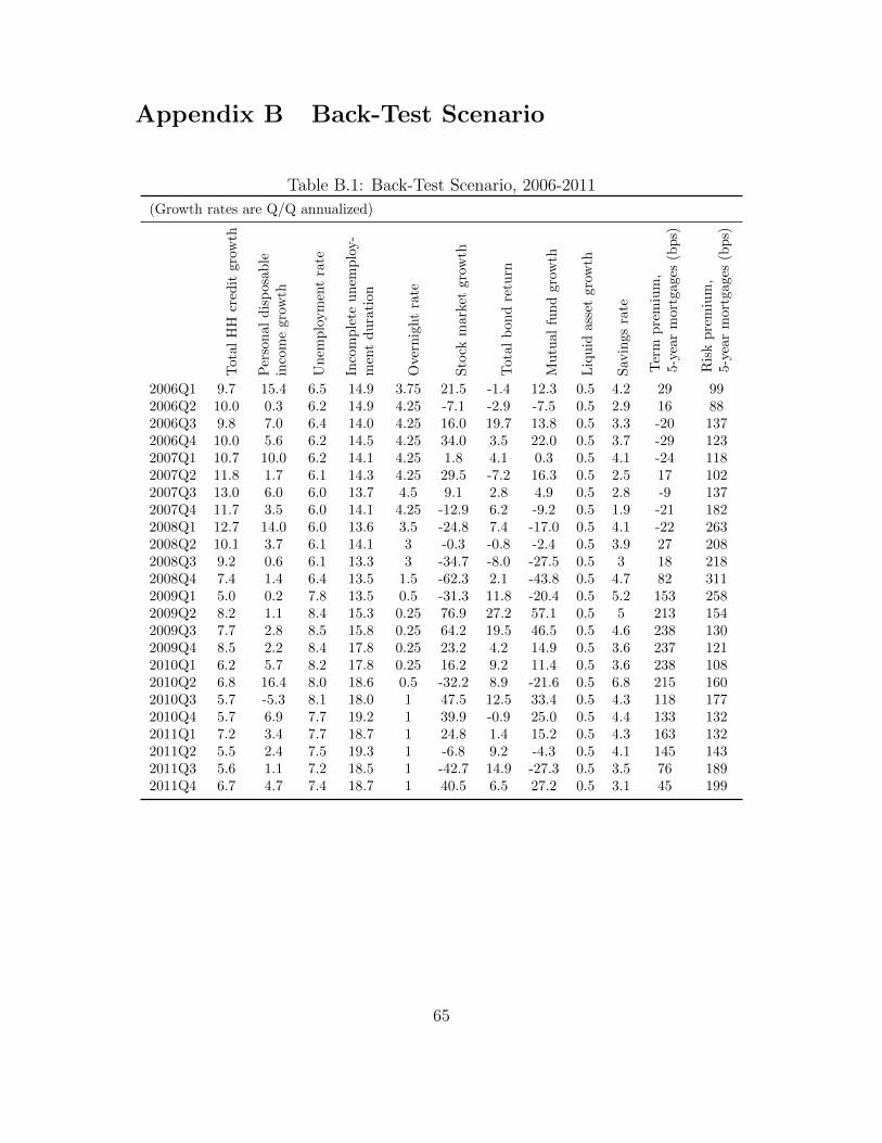
Appendix B Back-Test Scenario
Table B.1: Back-Test Scenario, 2006-2011
(Growth rates are Q/Q annualized)
Tota
lH
Hcr
edit
gro
wth
Per
son
aldis
pos
ab
lein
com
egr
owth
Un
emp
loym
ent
rate
Inco
mp
lete
un
emp
loy-
men
td
ura
tion
Ove
rnig
ht
rate
Sto
ckm
arket
grow
th
Tot
al
bon
dre
turn
Mu
tual
fun
dgro
wth
Liq
uid
asse
tgr
owth
Sav
ings
rate
Ter
mp
rem
ium
,5-y
ear
mort
gages
(bp
s)
Ris
kp
rem
ium
,5-y
ear
mort
gages
(bp
s)
2006Q1 9.7 15.4 6.5 14.9 3.75 21.5 -1.4 12.3 0.5 4.2 29 992006Q2 10.0 0.3 6.2 14.9 4.25 -7.1 -2.9 -7.5 0.5 2.9 16 882006Q3 9.8 7.0 6.4 14.0 4.25 16.0 19.7 13.8 0.5 3.3 -20 1372006Q4 10.0 5.6 6.2 14.5 4.25 34.0 3.5 22.0 0.5 3.7 -29 1232007Q1 10.7 10.0 6.2 14.1 4.25 1.8 4.1 0.3 0.5 4.1 -24 1182007Q2 11.8 1.7 6.1 14.3 4.25 29.5 -7.2 16.3 0.5 2.5 17 1022007Q3 13.0 6.0 6.0 13.7 4.5 9.1 2.8 4.9 0.5 2.8 -9 1372007Q4 11.7 3.5 6.0 14.1 4.25 -12.9 6.2 -9.2 0.5 1.9 -21 1822008Q1 12.7 14.0 6.0 13.6 3.5 -24.8 7.4 -17.0 0.5 4.1 -22 2632008Q2 10.1 3.7 6.1 14.1 3 -0.3 -0.8 -2.4 0.5 3.9 27 2082008Q3 9.2 0.6 6.1 13.3 3 -34.7 -8.0 -27.5 0.5 3 18 2182008Q4 7.4 1.4 6.4 13.5 1.5 -62.3 2.1 -43.8 0.5 4.7 82 3112009Q1 5.0 0.2 7.8 13.5 0.5 -31.3 11.8 -20.4 0.5 5.2 153 2582009Q2 8.2 1.1 8.4 15.3 0.25 76.9 27.2 57.1 0.5 5 213 1542009Q3 7.7 2.8 8.5 15.8 0.25 64.2 19.5 46.5 0.5 4.6 238 1302009Q4 8.5 2.2 8.4 17.8 0.25 23.2 4.2 14.9 0.5 3.6 237 1212010Q1 6.2 5.7 8.2 17.8 0.25 16.2 9.2 11.4 0.5 3.6 238 1082010Q2 6.8 16.4 8.0 18.6 0.5 -32.2 8.9 -21.6 0.5 6.8 215 1602010Q3 5.7 -5.3 8.1 18.0 1 47.5 12.5 33.4 0.5 4.3 118 1772010Q4 5.7 6.9 7.7 19.2 1 39.9 -0.9 25.0 0.5 4.4 133 1322011Q1 7.2 3.4 7.7 18.7 1 24.8 1.4 15.2 0.5 4.3 163 1322011Q2 5.5 2.4 7.5 19.3 1 -6.8 9.2 -4.3 0.5 4.1 145 1432011Q3 5.6 1.1 7.2 18.5 1 -42.7 14.9 -27.3 0.5 3.5 76 1892011Q4 6.7 4.7 7.4 18.7 1 40.5 6.5 27.2 0.5 3.1 45 199
65