IOWA STATE UNIVERSITY Department of Economics Ames, Iowa, 50011-1070

Iowa State University does not discriminate on the basis of race, color, age, religion, national origin, sexual orientation, gender identity, sex, marital status, disability, or status as a U.S. veteran. Inquiries can be directed to the Director of Equal Opportunity and Diversity, 3680 Beardshear Hall, (515) 294-7612.

Household Production Theory and Models

Wallace E. Huffman

Working Paper No. 10019June 2010

1

June 22, 2010

Household Production Theory and Models

By Wallace E. Huffmana/

Abstract: The chapter focuses on household production theory and models for non-agricultural households, largely in developed countries. The objectives of the paper are: (1) to present several types of microeconomic models of household decision making and highlight their implications for empirical food demand studies and (2) to presents an empirical application of insights gained from household production theory for a household input demand system fitted to unique data on the US household sector over the post-World War II period, 1948-1996. Regarding future research, suggestions are presented as to how food demand studies might build a stronger bridge to new models of household behavior, including a household production function and allocation of the household’s time and full-income constraints. . Key works: Households, production, models of behavior, input demand system, time allocation

a/The author is C.F. Curtiss Distinguished Professor of Agriculture and Life Sciences and Professor of Economics, Iowa State University. Jessica Schuring, Abe Tegene, Sonya Huffman, and Peter Orazem made helpful comments on an earlier draft. Alicia Rosburg provide extensive editorial suggestions. Also, this version has benefitted from an anonymous reviewer and the editors comments. Chiho Kim, Tubagus Feridhanusetyawan, Alan McCunn, Jingfing Xu and Matt Rousu also helped with data construction and estimation. Dale Jorgenson generously provided capital service price and quantity data for durable goods of the US household sector. The project is funded by the Iowa Agricultural Experiment Station and more recently by a cooperative agreement from the USDA-ERS.

2

Household Production Theory and Models I. Introduction Becker (1965) is best known for modeling household decisions and resource allocation in

a model where a household is both a producing and consuming unit. Output that is produced by

the household is consumed directly and not sold in the market. Becker claimed the productive

household model was a major advance in understanding household behavior relative to models

that treated households as purely consuming units (e.g., see Varian 1992, pp. 94-113). Margaret

Reid (1934) provided an early description of household production behavior, and her work is an

important antecedent to Becker’s formal modeling of the productive household. And in the early

1960s, Mincer (1963) became convinced of serious misspecification of empirical household

demand functions for food, transportation services, and domestic services; the opportunity cost

of the homemaker’s or traveler’s time and household non-labor (or full-) income were omitted

variables. He also showed that using cash income as an explanatory variable was inappropriate

because it reflected a variety of household decisions, including a decision on how many hours to

work for pay. Food economic studies over the past four decades have largely overlooked the

potential of household production theory and models in demand analysis.

This chapter first presents a brief review of empirical studies of food demand, especially

linkages to household production theory and models. However, the main objectives of the paper

are: (1) to present several types of microeconomic models of household decision making and

highlight their implications for empirical food demand studies and (2) to presents an empirical

application of insights gained from household production theory for a household input demand

system fitted to unique data on the US household sector over the post-World War II period,

3

1948-1996.1 Finally, I address how future food demand studies might build a stronger bridge to

the models of household behavior including a production function and resource of human time of

adult household members. The chapter focuses on household production theory and models for

non-agricultural households largely in developed countries.2

Relative to neoclassical demand functions, the models of productive household behavior

that are developed in this chapter include the opportunity cost of time of adults, full-income

budget constraint, and technical efficiency or technical change in household production as

determinants of the demand for food and other inputs. An important dimension of these models

is that time spent shopping, preparing and eating food has a cost even though there is not a direct

cash outlay and that individuals who have a higher opportunity cost of time find ways to

substitute toward less human time intensive means of household production.

The remainder of the paper is organized into four major sections.

II. A Brief Review of Demand Theory and Empirical Studies of Food Demand

Although LaFrance (2001) presents an abstract re-statement of neoclassical demand

theory and the theory of demand with household production, he does not present a review of the

empirical food demand literature, empirical applications or estimates of household demand

systems. Looking more broadly, I uncovered two papers that make a concerted effort to

incorporate household production theory into an empirical study of the demand for food. These

papers are by Prochaska and Schrimper (1973) and Hamermesh (2007). Prochaska and

Schrimper use cross sectional micro or household data to estimate the demand by households for 1 In contrast to Becker’s and Gronau’s perspective on household decision making, there is a sizeable literature that applies game theory or bargaining theory to two-adult household decision making, for example, see Blundell and MaCurdy (1999) and Browing et al. (2009). 2 For those who are interested in a conceptual model of agricultural household decision making where decisions are made on inputs for farm production and for household production, see Huffman and Orazem (2007, pp. 2286-2292), or agricultural household models that incorporate a time constraint and multiple job-holding of household members, see Huffman (1991, 2001, pp. 344-347) and Strauss (1986a). Empirical studies of food demand by agricultural households include Strauss (1986b) and Pitt and Rosenzweig (1986).

4

food-away-from home. The authors include a measure of the opportunity cost of time of the

homemaker or opportunity wage and a comprehensive measure of household income, computed

as the annual value of the homemaker’s time endowment evaluated at the market wage plus

household non-labor income. They found that an increase in the homemakers’ opportunity cost

of time and comprehensive household income significantly increased the demand for food-away-

from-home. They also show that significant specification bias would have occurred in the

estimated coefficients of the included variables if the opportunity cost of time had been excluded

or ignored.3

A recent study by Hamermesh (2007) builds on household production theory in his

empirical study of demand for food-at-home and away-from-home and time allocated to eating

by married couples in 1985 and 2003. Key explanatory variables are husband’s and wife’s wage

rates and a household’s non-labor income. He finds that a higher wage rate for the husband and

wife increase the demand for food-away-from-home significantly. Although the estimated effect

of the husband’s and wife’s wage rates on the demand for food-at-home are negative, only the

estimated coefficient for wife’s wage is significantly different from zero. In the 1985 data, he

found that non-labor income has a significant positive effect on the demand for food-at-home but

a negative effect on the demand for food-away-from-home. However, in the 2003 data, income

effects are reduced and much weaker than in the 1985 data.

Other food demand studies that incorporate household production theory are by Kinsey

(1983), Keng and Lin (2005), Park and Capps (1997) and Sabates et al. (2001).

Although Kinsey (1983) lays out a Beckerian model of household production in a study of the

demand for households’ purchases of food away from home, her empirical analysis she does not

3 Chen et al. (2002) did not find a statistically significant effect of an individual’s wage on the demand for particular nutrients—riboflavin, fatty acids and oleic acids—in the NHANES data set.

5

follow through. For example, she claims that the wage rates of working women do not vary

much and then excludes women’s price of time from a household’s demand for food-away-from-

home. In contrast, labor economists have made a working individual’s wage the target of

frequent empirical investigations, and predicted wage rates are regularly included in models

explaining labor supply, demand for children and migration (Card 1999, Tokle and Huffman

1991, Blundell and MaCurdy 1999, Huffman and Feridhanusetyawan 2007).

Keng and Lin (2005) show that as women’s labor market earnings increase their

household’s demand for food-away-from-home increases. In addition, a few other studies have

included the education of the household manager, a rough proxy for her opportunity cost of time,

as a regressor in food demand equations. For example, Park and Capps (1997) found that the

probability a household purchases ready-to-eat or ready-to-cook meals increases with the

education of the household manager, but education was not included in the expenditure equation

for ready-to-cook meals.

In new research at ERS, Andrews and Hamrick (2009) argue that “eating requires both

income to purchase food and time to prepare and consume it.” Their focus is on income effects:

“food spending tends to rise with a household’s income. However, the opposite is true for time

devoted to preparing food.” Their research does not focus on price effects. In conclusion, there is

not an abundance of evidence that productive household theory has been integrated into

econometric studies of food demand.

III. A Neo-Classical Model of Household Decisions to Allocate Human Time and Cash Income

Early models of labor supply decisions of household members made small advances in

neoclassical demand theory by adding leisure time to the list of goods that a household consumes

and by adding a new type of resource constraint—adult human time endowments that were

6

allocated between leisure and work for pay (Varian 1992, pp. 95-113, 144-146; Blundell and

MaCurdy 1999). This model provides an important benchmark by incorporating the opportunity

cost of time into household decision making, but it does not go so far as adding a household

production function. To see this, assume that the household consumes and obtains utility from

leisure (L) and two purchased goods—food (X1) and non-food goods and services (X2)—and

utility can be summarized by a strictly concave utility function

(1) U = U(L, X1, X2; τ).

In (1) τ is a taste parameter, affecting the translation of leisure and purchased goods into utility.

The household receives a time endowment each time period, e.g., year, and it is allocated

between leisure (L) and hours of work for pay (h):

(2) T= L + h.

The household receives cash income (IC) from members working for a wage (W) and from

interest, dividends and unanticipated gifts (V), and this income is allocated to purchasing X1 and

X2 such that

(3) IC = W·h + V = P1X1 + P2X2.

Although a household might choose to allocate all physical time to leisure and spend only V on

X1 and X2, most households choose to forego some leisure and to allocate this time to wage work,

in order to purchase larger quantities of X1 and X2. Under these conditions, I can rearrange

equation (2) to obtain h =T − L. Substitute this relationship into equation (3) and re-arrange to

obtain Beckerian (Becker 1965) full income (F) constraint

(4) F = W·T + V = W·L + P1X1 + P2X2. Note that full-income is received from the sale of part

of the time endowment at the wage rate (W) plus non-labor income (V), and hence, it does not

7

vary with hours of work. Moreover, full income received is spent on leisure and purchases of

food and non-food goods and services.

At this interior solution, the household chooses L, X1 and X2 to maximize equation (1)

subject to equation (4) with a Lagrange multiplier (λ), which is the marginal utility of full

income. These first-order conditions for the household’s decision problem are

(5a) L: UL = λW

(5b) Xi: iXU = λPi, i = 1, 2

(5c) λ: W·T + V − W·L − P1X1 − P2X2 = 0

Equations (5a)−(5c) can be solved jointly to obtain the general form of the household’s demand

functions for leisure, food, and non-food goods and services:

(5a) L* = DL(W, P1, P2, V, τ) = DL(W, P1, P2, F, τ)

(5b-c) X *i =

iXD (W, P1, P2, V, τ) = iXD (W, P1, P2, F, τ), i = 1, 2.4

Clearly, the demands for leisure, food purchases and non-food purchases are determined by the

wage rate, which is the price of leisure at an interior solution, the price of purchased food (P1),

the price of non-food purchases (P2), income (V or F) and tastes (τ). The income effect on

demand can be represented either by non-labor income (V) or as full-income (F), given that W,

which is the opportunity cost of time, is held constant in either case.

Given the optimal choice of leisure and the time constraint (2), obtain the general form of

the labor supply equation

(6) h* = T - L* = Sh(W, P1, P2, V, τ) = Sh(W, P1, P2, F, τ).

4 Although T is a determinant of demand, it is a constant that does not vary across household so it can be suppressed in the specification of the demand (and supply) functions.

8

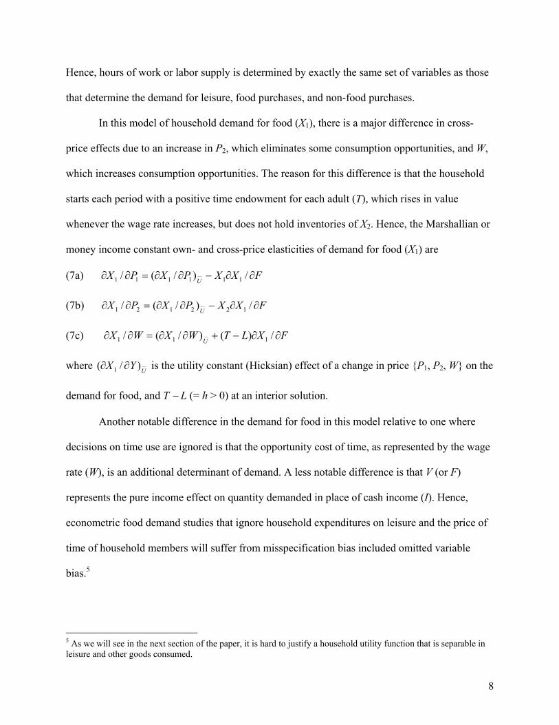
Hence, hours of work or labor supply is determined by exactly the same set of variables as those

that determine the demand for leisure, food purchases, and non-food purchases.

In this model of household demand for food (X1), there is a major difference in cross-

price effects due to an increase in P2, which eliminates some consumption opportunities, and W,

which increases consumption opportunities. The reason for this difference is that the household

starts each period with a positive time endowment for each adult (T), which rises in value

whenever the wage rate increases, but does not hold inventories of X2. Hence, the Marshallian or

money income constant own- and cross-price elasticities of demand for food (X1) are

(7a) FXXPXPXU

∂∂−∂∂=∂∂ /)/(/ 111111

(7b) FXXPXPXU

∂∂−∂∂=∂∂ /)/(/ 122121

(7c) FXLTWXWXU

∂∂−+∂∂=∂∂ /)()/(/ 111

where U

YX )/( 1 ∂∂ is the utility constant (Hicksian) effect of a change in price {P1, P2, W} on the

demand for food, and T − L (= h > 0) at an interior solution.

Another notable difference in the demand for food in this model relative to one where

decisions on time use are ignored is that the opportunity cost of time, as represented by the wage

rate (W), is an additional determinant of demand. A less notable difference is that V (or F)

represents the pure income effect on quantity demanded in place of cash income (I). Hence,

econometric food demand studies that ignore household expenditures on leisure and the price of

time of household members will suffer from misspecification bias included omitted variable

bias.5

5 As we will see in the next section of the paper, it is hard to justify a household utility function that is separable in leisure and other goods consumed.

9

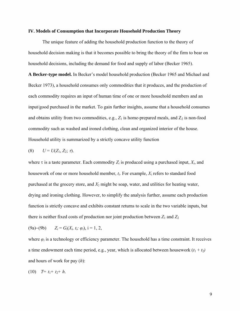
IV. Models of Consumption that Incorporate Household Production Theory The unique feature of adding the household production function to the theory of

household decision making is that it becomes possible to bring the theory of the firm to bear on

household decisions, including the demand for food and supply of labor (Becker 1965).

A Becker-type model. In Becker’s model household production (Becker 1965 and Michael and

Becker 1973), a household consumes only commodities that it produces, and the production of

each commodity requires an input of human time of one or more household members and an

input/good purchased in the market. To gain further insights, assume that a household consumes

and obtains utility from two commodities, e.g., Z1 is home-prepared meals, and Z2 is non-food

commodity such as washed and ironed clothing, clean and organized interior of the house.

Household utility is summarized by a strictly concave utility function

(8) U = U(Z1, Z2; τ).

where τ is a taste parameter. Each commodity Zi is produced using a purchased input, Xi, and

housework of one or more household member, ti. For example, X1 refers to standard food

purchased at the grocery store, and X2 might be soap, water, and utilities for heating water,

drying and ironing clothing. However, to simplify the analysis further, assume each production

function is strictly concave and exhibits constant returns to scale in the two variable inputs, but

there is neither fixed costs of production nor joint production between Z1 and Z2

(9a)−(9b) Zi = Gi(Xi, ti; φi), i = 1, 2,

where φi is a technology or efficiency parameter. The household has a time constraint. It receives

a time endowment each time period, e.g., year, which is allocated between housework (t1 + t2)

and hours of work for pay (h):

(10) T= t1+ t2+ h.

10

The household has a cash income constraint (I), which it receives a cash income from members

working for a wage (W) and from income on financial assets (interest and dividends) and

unanticipated gifts (V), and this cash income is allocated to purchasing X1 and X2

(11) I = W·h + V = P1X1 + P2X2.

In this model, I first examine household decision making in the input-space, i.e., to

choose inputs so as to maximize utility (8), subject to the production technology, physical time,

and cash income constraint. Moreover, if the household allocates physical time to work in the

market at wage rate (W), the physical-time (10) and cash-income constraints (11) can be

combined into one full-income constraint

(12) F = W·T + V = P1X1 + Wt1+ P2X2 +W·t2.

In addition, one method of incorporating the technology constraint is by substitution (9a)

and (9b) into (8). The new constrained optimization with Lagrange multiplier λ (marginal utility

of full income) becomes

(13) ψ = U[G1(X1, t1; φ1), G2(X2, t2; φ2); τ] + λ[W·T+ V − P1X1 − W·t1 − P2X2 − W·t2].

The first-order conditions for an interior solution is

(14a) Xi: iZUiiXG − λPi = 0, i = 1, 2

(14b) ti: iZUiitG − λW = 0, i = 1,2

(14c) λ: W·T+ V − W·L − P1X1 − P2X2 = 0,

where iZU is the marginal utility of commodity Zi, iiXG is the marginal product of input Xi in

producing Zi and iitG is the marginal product of input ti in producing Zi. A notable feature of

these first-order conditions in (14a) and (14b) is that for a household to maximize utility subject

to its technology and resource constraints, it must produce Z1 and Z2 at minimum cost

11

(15) ),,(// iiiitiiXZ PWGPGWMCiii

φπ=== , i = 1, 2.

iZMC = ),,( iii PW φπ is the marginal cost of Zi, which depends on the opportunity cost of time

(W), the price of purchased input (Pi), and the technology or efficiency parameter (φi). Moreover

with fixed input prices to the household and constant returns to scale in producing the Zi’s, the

marginal cost of producing each Zi is unchanged with a proportional re-scaling, e.g., doubling of

both variable inputs.

From equations (14a)−(14c), solve for the following general form of the implicit demand

functions for the inputs in this model

(16a) 2,1),,,,,,,(),,,,,,( 21212121* === iFWPPDVWPPDX

ii Xxi τφφτφφ

(16b) 2,1),,,,,,,(),,,,,,( 21212121* === iFWPPDVWPPDt

ii tti τφφτφφ

And, hence, the general form of the demand equations for housework and supply of labor can be

derived as follows

(17a) ),,,,,,(),,,,,,( 21212121*2

*1

* τφφτφφ FWPPDVWPPDtttpp ttp ==+=

(17b) ),,,,,,(),,,,,,( 21212121*2

*1

* τφφτφφ FWPPSVWPPSttTh HH ==−−= .

Moreover, the demand for purchased inputs, such as food, housework, and labor supply are all a

function of the prices (Pi’s) of purchased inputs for home production [such as meat and fish;

potatoes, pasta, bread; tomatoes, lettuce, cucumbers; and milk and eggs], price of housework

(W), non-labor or full income (V or F), the technology or efficiency parameters (φ1and φ2), and

the taste parameter (τ).6 Hence, with the household production model the education of the

homemaker can be connected to the efficiency of household production (φi) and not be forced

6 In contrast, if we assume the technology of household production is represented by a joint production function, G(Z1, Z2, X1, X2, tp, φ) = 0, with Zs as commodities (outputs); X s and tp as inputs, and efficiency parameter φ, where G(· , φ ) is convex in outputs, decreasing in inputs, and strictly increasing in Z1, then we obtain roughly the same implicit input demand functions as in (16a) and (17a) and supply function as in (17b).

12

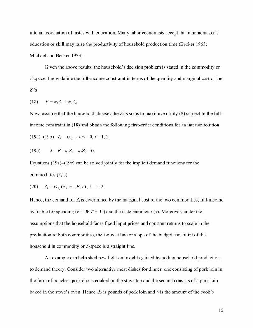
into an association of tastes with education. Many labor economists accept that a homemaker’s

education or skill may raise the productivity of household production time (Becker 1965;

Michael and Becker 1973).

Given the above results, the household’s decision problem is stated in the commodity or

Z-space. I now define the full-income constraint in terms of the quantity and marginal cost of the

Zi’s

(18) F = π1Z1 + π2Z2.

Now, assume that the household chooses the Zi ’s so as to maximize utility (8) subject to the full-

income constraint in (18) and obtain the following first-order conditions for an interior solution

(19a)−(19b) Zi: iZU - λπi = 0, i = 1, 2

(19c) λ: F - π1Z1 - π2Z2 = 0.

Equations (19a)−(19c) can be solved jointly for the implicit demand functions for the

commodities (Zi’s)

(20) Zi = ),,,( 21 τππ FDiZ , i = 1, 2.

Hence, the demand for Zi is determined by the marginal cost of the two commodities, full-income

available for spending (F = W·T + V ) and the taste parameter (τ). Moreover, under the

assumptions that the household faces fixed input prices and constant returns to scale in the

production of both commodities, the iso-cost line or slope of the budget constraint of the

household in commodity or Z-space is a straight line.

An example can help shed new light on insights gained by adding household production

to demand theory. Consider two alternative meat dishes for dinner, one consisting of pork loin in

the form of boneless pork chops cooked on the stove top and the second consists of a pork loin

baked in the stove’s oven. Hence, Xi is pounds of pork loin and ti is the amount of the cook’s

13

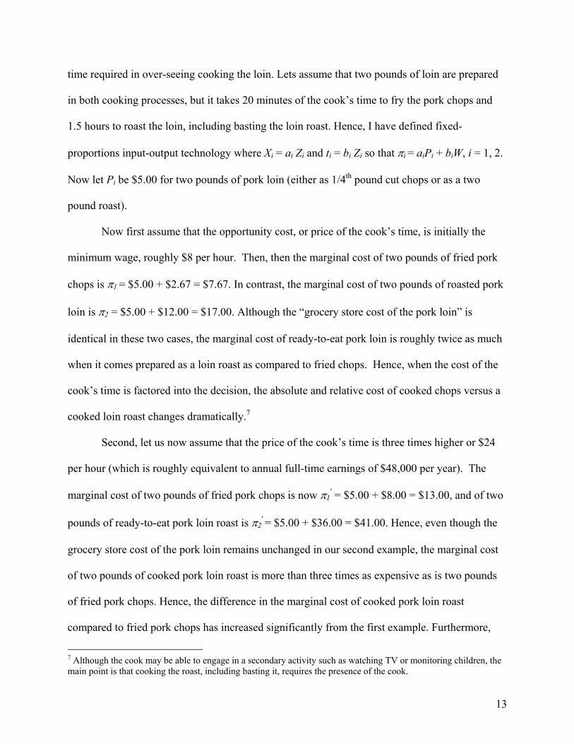
time required in over-seeing cooking the loin. Lets assume that two pounds of loin are prepared

in both cooking processes, but it takes 20 minutes of the cook’s time to fry the pork chops and

1.5 hours to roast the loin, including basting the loin roast. Hence, I have defined fixed-

proportions input-output technology where Xi = ai Zi and ti = bi Zi so that πi = aiPi + biW, i = 1, 2.

Now let Pi be $5.00 for two pounds of pork loin (either as 1/4th pound cut chops or as a two

pound roast).

Now first assume that the opportunity cost, or price of the cook’s time, is initially the

minimum wage, roughly $8 per hour. Then, then the marginal cost of two pounds of fried pork

chops is π1 = $5.00 + $2.67 = $7.67. In contrast, the marginal cost of two pounds of roasted pork

loin is π2 = $5.00 + $12.00 = $17.00. Although the “grocery store cost of the pork loin” is

identical in these two cases, the marginal cost of ready-to-eat pork loin is roughly twice as much

when it comes prepared as a loin roast as compared to fried chops. Hence, when the cost of the

cook’s time is factored into the decision, the absolute and relative cost of cooked chops versus a

cooked loin roast changes dramatically.7

Second, let us now assume that the price of the cook’s time is three times higher or $24

per hour (which is roughly equivalent to annual full-time earnings of $48,000 per year). The

marginal cost of two pounds of fried pork chops is now π1′ = $5.00 + $8.00 = $13.00, and of two

pounds of ready-to-eat pork loin roast is π2′ = $5.00 + $36.00 = $41.00. Hence, even though the

grocery store cost of the pork loin remains unchanged in our second example, the marginal cost

of two pounds of cooked pork loin roast is more than three times as expensive as is two pounds

of fried pork chops. Hence, the difference in the marginal cost of cooked pork loin roast

compared to fried pork chops has increased significantly from the first example. Furthermore,

7 Although the cook may be able to engage in a secondary activity such as watching TV or monitoring children, the main point is that cooking the roast, including basting it, requires the presence of the cook.

14

this logic can be used to explain why wealthy households tend to consume expensive easy to

prepare cuts of meat rather than cheap time consuming to prepare ones. When the cost of the

cook’s time tripled, the marginal cost of the time-intensive pork loin roast increases relative to

the marginal cost of the fried pork chops—from 17/6.67 = 2.55 in the first example to 41/13 =

3.15 in the second example. Hence, as the price of the cook’s time increases, the marginal cost of

cook’s-time-intensive pork meals increases relative to those that are less intensive in cook’s

time—fried pork chops. Viewed another way, as women have obtained more education and

entered the labor force, which increases the opportunity cost of their time, cook’s-time intensive

meal preparation has become less attractive. Given that meals prepared at home are on average

more nutritious than meals eaten away from home, this change has a negative impact on the

production of good health (Lin et al. 1999). See application at the end of this section.

A second factor that weighs against pork loin roasts is that the minimum size is about two

pounds, which would feed a relatively large household (or a dinner party), and as average

household sizes declined over the 1950s and 1960s, households are more likely to be too small to

make roasting a loin economical and fried pork chops become more likely. However, frying pork

chops in cooking oil, which means adding oil and calories per oz of prepared meat, is widely

recognized as a less healthful means of preparing loin than the more time intensive oven-

roasting.8 Given that women continue to be the main meal planners and preparers, these

examples show how rising opportunity cost of women’s time has tipped the scale toward less

healthy meal preparation for household’s members (Kerkhofs and Kooreman 2003, Lin et al.

1999, Robinson and Godbey 1997) .

8 Basting liquid for pork loin roasts also consist of some vegetable oil, but also wine and spices. However, a much smaller share of the loin comes in direct contact with the oil than in fried pork chops, which reduces oil uptake.

15

After replacing fixed- for variable-proportions production technology, additional insights

from the Becker model of household production are obtained. To do this, continue with the two

commodity-two input model. Moreover, assume that X = X1 + X2, i.e., the purchased inputs are

perfect substitutes, and continue with total time in housework allocated between t1 and t2. In

addition assume that commodity Z2 is relatively time intensive to produce, and the prices of the

purchased component of production of each Z (Pis) is fixed to the household. Given the

assumption of constant returns to scale in the production of both commodities, all of the

information about production of each commodity can be represented on a unit isoquant, i.e., Zi =

1. Total production involves only rescaling the information in the unit isoquant model.

Consider Panel A, Figure 1 where the initial iso-cost line C0 with slope (- W/P) is

drawn tangent to the one-unit isoquant for Z1 and Z2 at a and b. Because I will focus on the

implications of an increase in the wage rate, I will measure cost in term of units of X, which is

unchanged in our example. Hence, in the initial situation, the cost of one unit of Z1 and Z2 is 0C0

in units of X. An increase in the wage rate from W to W ‘ while minimizing cost causes a

substitution effect away from time (ti) toward the purchased input component (Xi) and the

marginal cost of both Z’s increases in units of X—to 0C11 for Z1 and to 0C12 for Z2. However, the

marginal cost of Z2, which is relatively time intensive, rises relative to the marginal cost of Z1.

Next, consider the effect of an increase in the wage rate (W) in commodity or Z- space.

The initial budget constraint is R0 with tangency to U0 at a and with optimal quantities of

and in Figure 1, Panel B. I have already shown that when the wage rate increases, the

marginal cost/price of the time intensive commodity Z2 increases relative to the marginal cost of

the less time intensive commodity Z1 (Figure 1, panel A).9 The new relative marginal cost-price

9 This is an application of the Lerner-Pearce Diagram from international trade theory (Lerner 1952, Deardorff 2002).

16

line for the Z’s is R1 tangent to U0 at point b in Figure 1, Panel B. Given that the production of

both Z’s uses purchased inputs and housework, the household will experience a net increase in

consumption opportunities as a result of the increase in the wage rate and a new budget

constraint of R2 . Hence, the increase in consumption opportunities is represented by the area

R1R2 , and the household can now move to any point between j and l on R2 . Even with a

pure substitution effect away from the housework-intensive commodity Z2 as the wage increases,

that the consumption of Z2 will actually increase. This occurs when the new optimum between j

and k on R2 . However, if the new optimum is located between k and l on R2 , the quantity

demanded of Z2 will decline. In addition, there is a high probability that the consumption of Z1

will increase.

Becker’s model of household production has been criticized because of his assumption of

constant returns to scale in producing each commodity (the Z’s) and the assumption of no joint

production in producing the Z’s, for example see Pollak and Wachter (1975). However, these

assumptions are only needed to obtain a straight line iso-cost constraint or budget constraint,

which implies that household preferences and the budget constraint are independent.

Additional insights can be obtained by considering the following model of joint

production. Assume the household obtains utility directly from consuming Z1, which is produced

using use X1 and t1, as in equation (9a), but t1 also provides utility (or disutility) directly to the

household. For example, time cleaning the house or doing the laundry may directly lower utility

but time gardening may directly raise utility, irrespective of the utility obtained from the product

produced. Hence, the household’s strictly concave utility function can be written as

(21) U = U(Z1, t1; τ).

The household’s time constraint is

17

(22) T = t1+ h,

and the full-income budget constraint is

(23) W·T + V − P1X1 − W·t1 = 0.

The household now chooses X1 and t1 so as to maximize (21) subject to the technology of

producing Z1 and the full-income constraint

(24) ψ = U[G1(X1, t1; φ1), t1;τ]+ λ[W·T + V − P1X1 − W·t1].

The first-order conditions at an interior solution are

(25a) X1: 011 11=− PGU XZ λ

(25b) t1: 0111 1 =−+ WUGU ttZ λ

(25c) λ: W·T + V − P1X1 − W·t1 = 0

where 1t

U represents only the direct contribution of t1 to utility. Rearranging equations (25a) and

(25b) provides important information about optimal input combinations for producing Z1

(26) 111 /)/(/111

PUWGG tXt λ−= .

First, if t1 does not directly enter the household utility, i.e., 1t

U = 0, then obtain the

standard result for producing at cost minimization, or point a in Figure 2. If instead, the

household obtains positive utility directly from housework, e.g., the homemaker enjoys cooking

or gardening, then the direct impact of housework on utility is positive, 1t

U > 0, and the optimal

input combination will be at point b in Figure 2, which implies that more time will be devoted to

cooking or gardening than when pure cost minimization reigns. In contrast, if the household

obtains negative utility directly from housework, e.g., the homemaker dislikes cleaning the house

and doing the laundry, then direct effect of housework on utility is negative, 1t

U < 0, and the

optimal input combination will be at point c in Figure 2, which implies that less time will be

18

devoted to cleaning or doing the laundry than when cost minimization reigns. Clearly, this

substitution toward more X1 in producing could include hiring a home cleaning service or

taking clothing to a commercial laundry for washing and ironing.

A Gronau-type model. The most notable feature of the Gronau model of household production

is that home produced and purchased goods are perfect substitutes, but this could also be one of

its shortcomings (Gronau 1977, 1986). Assume a household consumes and obtains utility from

two goods, leisure (L) and a good X, say meals, which can be produced at home, denoted as X1 or

purchased in the market, denoted X2. In Gronau’s framework, these goods are assumed to be

perfect substitutes, where the household only values total X rather than individual quantities of

home produced and purchased X

(27) X = X1 + X2.

Also, the household has a strictly concave utility function

(28) U = U(L, X; τ)

and for simplicity, assume that the household’s production function for X1 is strictly concave in

one variable input, housework (h1):

(29) X1 = G1(h1; φ)

Where φ is a technology or efficiency parameter. The household faces a time constraint,

receiving an endowment T each period that is allocated to leisure (L), housework (h1) and wage

work (h2):

(30) T = L + h1 + h2.

The household has cash income from wage work (h2) and non-labor income V, allocates it to X2

(31) I = W·h2 + V = P2X2.

19

Equation (30) can be solved for h2 and substituted into equation (31) to obtain the household’s

full-income constraint:

(32) F = W·T+ V = W·L + W·h1 + P2X2.

Equation (29) can be substituted into (27), which in turn is substituted into (28), and h1 and X2

can be chosen to maximize the modified utility function subject to the full-income constraint

(33) )(];);(,[ 221211 XPhWLWVTWXhGLU −⋅−⋅−+⋅++= λτφψ .

The first-order conditions for an interior solution are

(34a) L: LU – λW = 0

(34b) h1: 011 =− WGU hX λ

(34c) X2: 02 =− PU X λ

(34d) λ: ⋅W T .0221 =−⋅−−+ XPhWWLV

Combining equations (34b) and (34c), obtain the result that X1 should be produced under the

standard one-variable input profit maximizing condition, ,112 WGP h = and the general form of the

optimal quantity of housework demanded, t1, and supply of X1 is given by

(35a) *1h =

1tD ),,( 2 φPW

(35b) *1X = );( *

11 φhG = ),,( 21φPWS X .

Conditions (34a), (34c) and (34d) can be solved jointly for the following demand functions for

L* and *2X

(36a) L* = DL(W, P2, V, τ, φ) = DL(W, P2, F, τ, φ)

(36b) *2X = ),,,,( 22

φτVPWD X = ),,,,( 22φτFPWDX .

Rearranging the time constraint (30) and using the information in equations (35a) and (36a),

obtain the general form of the household’s labor supply equation

20

(37) h2 = *1

* hLT −− = S2h ( W, P, V, τ, φ) = S

2h ( W, P, F, τ, φ).

Figure 3 displays a graphic representation of the optimal resource allocation at an interior

solution for the Gronau model of household production. Units of X are on the vertical axis and

units of time are on the horizontal axis, but the maximum length of this axis is T, which is

reflected by the erection of a vertical line at this amount of human time. The household can

purchase XB units of X from its non-labor income (V). At point B on the vertical axis T, the

household considers how best to allocate a unit of time: to produce X directly or to work for a

wage and purchase the added X from earnings. The boundary of the technology and resource

constraints facing the household being represented by A1GB0h in figure 3. Moreover, figure 3 is

drawn such that at point B, the marginal product of housework in producing X (11hG ) is greater

than the real wage (W/P2), so it is optimal for the household to allocate time to housework rather

than wage work along the production relationship as the segment AGB. At point G optimal

housework is . This results in the quantity XB - XG of home produced goods. Additional

foregone leisure should be allocated to wage work since the figure the marginal product of

housework in producing X is lower than the real wage. The household’s utility maximum (U0)

occurs at e, with Xe - XG of X purchased from earnings. In the figure, the optimal amount of

leisure is L0 and of wage work is = L0 - .

An usual prediction of this model is that if non-labor income (V) increases, the

household will optimally keep the quantity of home produced goods (X1) unchanged, but allocate

the additional income to purchase units of X in the market (X2) and leisure (L). However, if P2

increases, this reduces the real wage rate (W/P2) and unambiguously increases the amount of

time allocated to and quantity of home-goods produced. The net impact on leisure, hours of work

and total quantity of X consumed will be determined by resulting substitution and income effects.

21

In this model, it is also obvious that an increase in the efficiency of producing X1 at all h, e.g.,

due to better information or training in home production, will increase the amount of time

allocated to and production of home goods (X1).

Application of Household Production Theory to Health with Food as an Input

Of considerable interest is the household’s production of good health, especially as it

related to obesity and associated health problems (Center for Disease Control (CDC) 2003,

Finkelstein et al. 2003, Huffman et al. 2009). Inputs in the health production function include

food, which is a source of protein, energy, vitamins, minerals, fiber; leisure time and medical

care. However, food intake also frequently yields utility directly because food texture and taste

gives satisfaction and eating and drinking together are a major part of satisfaction yielding social

interaction.

Let’s assume a household has a strictly concave utility function

(38) ),;,,,,( ZHLOLPCXHUU e=

where utility U depends on the current health status of the household members (H); consumption

of food and drink (X), other purchased goods (C) (excluding purchased health care); and

physically active leisure (LP) and other leisure time (LO). The variable eH represents early

health status, e.g., genetic potential for good/bad health or sometimes summarized by health

status at birth such as birth weight (Fogel 1994). Z denotes fixed observables, such as education,

gender, and race-ethnicity of adults. Current health, other purchased goods and other leisure

time (H, C and LO) are assumed to be positive “goods,” i.e., a marginal increase in any one of

them directly increases household utility ( LOCH UUU ,, > 0) and, hence, better (current) adult

health status increases household utility, as do higher consumption of other purchased goods and

more time allocated to sedentary leisure, e.g., TV viewing, surfing the web. However, time

22

allocated to vigorous physically active leisure may directly reduce utility, i.e., adults find this

activity unpleasant or uncomfortable and then ULP < 0.

Let’s assume the household’s production function for adult health status is

(39) H = ( , , ; , , )eH LP X I H Z ϕ ,

where H(·) is a strictly concave function and I is a vector of purchased health inputs or medical

care. The parameter ϕ summarizes unobservable factors which affect the efficiency of current

production of health status, e.g., genetic pre-disposition for good/bad health such as obesity. In

the health production function, I expect ILP HH , > 0, or holding other factors constant,

additional time allocated to physically active leisure (LP) or a larger quantity of purchased health

care (I) produces more good health. Although many adults may obtain disutility from vigorous

physically active leisure, the fact that its marginal product in health production is positive can

result in a combined direct and indirect effect on marginal utility ( LPLPHSLP UHUU += > 0) if the

positive first term on the right in this equation ( LPH HU ) outweighs a negative second term

( LPU ).

The marginal product of food in health production ( XH ) is expected to be positive for

some foods (i.e., XH > 0) and perhaps negative for others (i.e., XH < 0). For example, fresh

fruits and vegetables, which are high in fiber, vitamins and minerals, are expected to have a

positive marginal product on health output, but the marginal product might be negative for

processed fruits and vegetables, which frequently contain “added sugar” and sometimes contain

“added salt and fat” and less fiber and fewer vitamins and minerals than fresh produce. All meats

and fish contain protein which is essential for cell reproduction and growth, but they also contain

fat. Since fats are very calorie dense, they can contribute to excess energy intake and obesity.

Also, some fats detract (low density ones) from cardiovascular health and others are neutral or

23

positive (high density ones) to cardiovascular health. But, some fat is needed to make fresh

vegetables more palatable and to dissolve essential vitamins. Also, fat makes some other foods

taste “good,” which implies that the direct effect of X on utility is positive or UX > 0. If a type of

food has a negative marginal product in the production of good health, the combined marginal

effect of X on utility may still be positive, provided that XXHSX UHUU += > 0, or the first term

on the right of this equation ( XH HU ) is outweighed by a positive second term on the right (UX).

Assume the household has two adults and the time constraint consists of a time

endowment (T) which is allocated among work for pay (R), physically active leisure (LP) and

other leisure (LO): T = R + LP + LO. Let , ,X I CP P P denote the price vectors corresponding to X,

I and C, respectively, W denotes the wage rate or opportunity cost of time of an adult, V denotes

household non-labor income, then household cash income constraint WR + V is spent on X, I, and

C such that WR + V = PX X + PI I + PC C. Now household’s decision is to choose LP, LO, R, X, I

and C to maximize household utility subject staying within the human time and cash income

constraints

(40) , , , , ,max ( ( , , ; , , ), , , , ; , )

. . , 0, 0, 0

e eLP LO R X I C

X I C

u U H LP X I H Z X C LP LO H Z

s t P X P I P C WR VR LP LO T R LP LO

ϕ=

⋅ + ⋅ + ⋅ = +

+ + = ≥ ≥ ≥

where the first constraint is the household’s cash income constraint and the second constraint is

the household’s time constraint. The Lagrangian for the constrained utility maximization is

(41) = ( ( , , ; , , ), , , , ; , )

( ) ( )e e

X I C

U H LP X I H Z X C LP LO H ZWR V P X P I P C T R LP LO

ϕλ μ

Φ+ + − ⋅ − ⋅ − ⋅ + − − −

whereλ and μ are the Lagrange multipliers, indicating the marginal utility of cash income

(WR+V) and marginal utility of the time endowment (T), respectively.

24

The first-order conditions for an optimum, including Kuhn-Tucker conditions on LP and

R are

* * * *

* * * * * *

*

*

*

*

: 0 ( ) 0 0

: 0 ( ) 0 0:

:

:

:

:

H LP LP H LP LP

LO

H X X X

H I I

C C

X

LP U H U LP U H U LP

R W R W RLO U

X U H U P

I U H P

C U P

P X

μ μ

λ μ λ μ

μ

λ

λ

λ

λ

⋅ + − ≤ ⋅ ⋅ + − = ≥

⋅ − ≤ ⋅ ⋅ − = ≥

=

⋅ + =

⋅ =

=

⋅ * * * *

* * * : I CP I P C WR V

R LP LO Tμ

+ ⋅ + ⋅ = +

+ + =

where UH = ∂U/∂H, ULP = ∂U/∂LP, UC = ∂U/∂C, ULO = ∂U/∂LO, UX = ∂U/∂X, HLP = ∂H/∂LP, HX = ∂H/∂X and HI = ∂H/∂I represent partial derivatives.

These immediately above first-order conditions can be solved jointly for an interior

solution (where the opportunity cost of time is W) to obtain the implicit household optimal

demand function for LP, LO, X, I, and C:

LP* = LP(W, PX, PI, PC, V, He, Z, φ)

LO* =LO(W, PX, PI, PC, V, He, Z, φ)

(42) X* = X(W, PX, PI, PC, V, He, Z, φ)

I* = I(W, PX, PI, PC, V, He, Z, φ)

C* = C(W, PX, PI, PC, V, He, Z, φ).

Now upon substituting the equations in (42) into the health production function (39), obtain the

general form of the household’s health supply (and demand) function for (current) adult health:

(43) H* = H(LP*, X*, I*; He, Z, φ) = H(W, PX, PI, PC, V, He, Z, φ).

A notable feature of (43) is that it contains the same set of explanatory variables as those in the

the system of household demand equations (42). See Chen and Huffman (2009) for application

25

of this model to adults’ decisions to participate in physical activity and to be a healthy weight

(not obese).

V. An Empirical Application: Demand for Food-at-Home and Other Household Inputs

To more vividly illustrate the empirical implications of household production theory and

models for household demand studies, I consider the demand for inputs by the US sector over the

post-World War II period. The methodology that I follow is best described as a hybrid version of

Becker’s and Gronau’s productive household models in which there are two classes of unpaid

human time—unpaid housework and leisure, and where purchased and home-produced goods are

not perfect substitutes. Following Jorgenson et al. (2001), Jorgenson and Stiroh (1999) and

Jorgenson and Slesnick (2008), inputs are defined are defined as flows, and, hence, the input

from housing, household appliances, transportation equipment, recreation equipment is capital

services and not the durable goods themselves.10

The immediate post-World War II period is interesting because it was a time when the

war effort that had been directed to producing tanks, planes, ships, guns and ammunition was re-

directed to supplying durable goods—new houses, household appliances, and cars—to the

household sector and tractors and machinery for the farm sector. Moreover, major series on the

services of household durable goods are available from Jorgenson start in 1948. My period of

analysis ends in 1996, which is almost a half-century in length, and is a date when the transition

of women from housework to market work had been largely completed (Goldin 1986).

After translating durable goods into services, it is now plausible to specify a static

household input demand system that is in the spirit of equations (16a) and (17a), where leisure

10 Although capital services are proportional to the stock of consumer durables, proper aggregation requires weighting the stocks by rental prices rather than asset acquisition prices (Jorgenson et al. 1987). Moreover, the rental price for each asset incorporates the rate of return, the depreciation rate, and the rate of change in the acquisition price.

26

time is one of the ti’s. Over the post-World War II period, major changes in households included

less time allocated by women to preparing meals and meal clean-up at home and more meals

consumed away from home. Frequently, workday lunches are purchased and eaten at school or

work and weekend dinners are eaten in restaurants. When meals are at home, ready-to-eat food

is frequently purchased at fast-food restaurants, grocery delis and restaurants and taken home to

be eaten. Advances in household appliances now provide microwave ovens with timers and

electric and gas ranges with thermostatically controlled burners and ovens give temperature

control with little supervision, which may lead to higher-quality home produced meals. These

appliances are technically advanced relative to the coal, wood, kerosene and LP gas burning

cooking stoves of the late forties (Bryant 1986).11

Specific Input Groups

Nine empirical input categories are distinguished for the aggregate household sector and

indexes of price and quantity are constructed for each of them. Table 1 contains a brief definition

all variables used in the empirical demand system. A very brief some of some key details about

the input categories are discussed here, but greater details are available in Huffman (2008). As

indicated above, households’ durable goods are converted into service flows and personal

consumption expenditures on non-durables are used in constructing measures of non-durable

goods or inputs. Also, considerable evidence exists that unpaid housework of women and men

are not perfect substitutes, ranging from child care and meal planning and preparation where

women’s work dominates effort and to yard and car care and snow removal when men’s work

dominates effort (Becker 1981, Gronau 1977, Robinson and Godbey 1997, Bianchi et al. 2000,

11 An alternative perspective of these input demand functions is that they represent demand functions for goods and services that yield utility directly to households (Pollak and Wachter 1975).

27

Equiar and Hurst 2006, table 2 and 3). Hence, men’s and women’s time are treated as different

inputs.

The choice of exactly nine input groups is subjective, this is a large enough number to

provide large amounts of information about the structure of US household production and it is

near the maximum number of input categories can be supported in an econometric model with

the data at hand. The complete set of input categories is: (i) women’s (unpaid) housework, (ii)

men’s (unpaid) housework, (iii) food-at-home, (iv) purchased housework-substitute services

(e.g., domestic services, laundry and dry-cleaning services, and food-away-from-home), (v)

housing services (for owner-occupied and rental housing), (vi) services of household appliances

(including imputed services from computers, furnishings owned and household utilities), (vii)

transportation services (imputed services of transportation capital owned, purchased

transportation services, and fuel for transportation), (viii) recreational services and entertainment

(imputed services of recreation capital owned and recreation services purchased), and (ix) other

goods and services (largely men’s and women’s leisure) and other purchased services.12 Hence,

in this empirical framework, unpaid housework and “other” inputs, which is largely leisure time,

are distinct input categories.13,14

For this study, the daily time endowment of adults is rescaled from 24 hours to a

modified time endowment of 14 or 15 hours per day, by excluding time allocated to sleeping,

eating and other personal care. No evidence exists that time allocated to personal care by women

and men is responsive to prices or income, or even to trend (see Robinson and Godbey 1997, p.

12Some might suggest that food-away-from-home be treated as a separate input category, but for the early part of the study period, its share was quite small. See Prochaska and Schrimper (1973) for evidence. 13 Only one price exists for men’s and one for women’s time, and hence, it is not possible to include leisure time as a separate input. However, men’s and women’s leisure do account for more than 85% of the “other input” category. 14 Jorgenson and Slesnick (2008) use a household demand system consisting of four groups (nondurables, capital services, consumer services, and leisure). In particular, they do not distinguish between unpaid housework and true leisure and label the aggregate of the two leisure.

28

337).15 Moreover, Ramey (2005) and Greenwood et al. (2005) use similar modified time

endowments of roughly 100 hours per week in developing national economy macro

simulation/calibration models.

Each individual aged 16 and older who is not in school, is assumed to allocate his/her

modified time endowment among unpaid housework, labor market work, including commuting,

and leisure. Housework is defined as time allocated primarily to: food preparation and clean-up;

house, yard, and car care; care of clothing and linens; care of family members; and shopping and

management. Thus, housework in this study is considerably broader than “core housework”—

cooking, cleaning and washing dishes, doing the laundry, and cleaning and straightening the

house. Labor market work includes work for pay and commuting time to work. Time allocated

to leisure or free time is time allocated primarily to social organizations, entertainment,

recreation and communications.16 However, it is defined residually for each individual as his/her

allocatable time endowment less hours of housework and hours of labor market work.

The (modified) time endowment is set as follows. For women and men aged 16 to 64

who are not enrolled in school, the modified endowment is assumed to be 14 and 15 hours per

day, respectively. The size of these modified time endowments is based on information presented

in Robinson and Godbey (1997, p. 337) and Juster and Stafford (1991, p. 477) showing that

women spend a little more time on sleep and personal care than men. For women and men who

are 65 years of age and older, the modified time endowment is 13 and 14 hours, respectively.

The small reduction relative to individuals 16-64 years of age reflects that additional time is

15 However, technical change associated with showering/bathing—soaps, shampoos, deodorants, shaving equipment—has made it possible for steady increases in the quality of personal hygiene, with a roughly unchanged amount of time spent on personal care. 16 In empirical research, Juster and Stafford (1985, 1991) also distinguish between time allocated to housework and leisure. For the purposes of my study, it is important to maintain these distinctions for the primary uses of nonmarket time.

29

spent recovering from illnesses.17 In deriving aggregate average hours of paid work and of

unpaid housework, a distinction is made between the number of employed and not employed

women and men because these numbers have changed dramatically over time, which is a major

factor in re-allocation of adult time (see Huffman 2008).

Annual hours of unpaid housework for working and nonworking women and men aged

16-64, who are not in school, and for age 65 and over were derived from benchmark data. Hours

of work for pay were obtained from U.S. Department of Labor data files.18 Data on commuting

time were derived from information reported in Robinson and Godbey (1997). Hours of

women’s and men’s leisure are computed as the adjusted time endowment less hours of unpaid

housework, and hours of work for pay, including time for commuting to work. Among men and

women aged 16-64 who are not in school, women on average have slightly less leisure time than

men, but for men and women, the average amount of leisure time rose over 1948 to 1975, and

then decreased a little.

The price of time allocated to housework and leisure is defined as the foregone market

wage following procedures in Smith and Ward (1985) where an adjustment downward occurs in

the wage for the not-employed groups. An average nominal wage rate over working and not-

working men (and women) is constructed as the weighted-average of the average nominal wage

rate for employed and not-employed men (and women), which is an index number solution to the

aggregate problem. See Huffman (2008) for details.

Consumers purchase nondurable goods and services for consumption and acquire

consumer durables in order to obtain a flow of services to use in household production. Capital

services are proportional to the stock of assets, including computers, but aggregation requires

17 All computations dealing with time use assume a 365-day and 52-week year. 18 The derived annual average hours of labor market work are consistent with the Census year estimates presented by McGrattan and Rogerson (2004).

30

weighting the stocks by rental prices rather than acquisition prices for assets. The rental price for

each asset incorporates the rate of return, the depreciation rate, and the rate of decline in the

acquisition price. The Bureau of Economic Analysis (BEA) provides data on purchases of 12

types of consumer durable goods used in the construction of service measures for household

durable goods.

Input price indexes are Tornqvist indexes (Diewert 1976; Deaton and Muellbauer 1980a,

pp. 174-175). This index permits substitution to occur within major input categories as relative

prices of subcomponents change. The overall price index for the nine-input group making full-

expenditures is, however, the Stone price or cost of living index (Stone 1954).

Mean Values and Long-Term Trends over the Post-World War II Period

Mean per capital full-income-expenditure per capita over the study period is $4,369 in

1987 dollars. The mean expenditure share on women’s unpaid housework is 0.119, men’s unpaid

housework is 0.069, food-at-home is 0.052, purchased-housework-substitute services is 0.015,

housing services is 0.030, household appliance services is 0.030, transportation services is 0.047,

recreation services and expenditures is 0.025 and “other inputs” is 0.595. Given that the other

input category is dominated by leisure, the US household sector allocates a large share of full-

income to leisure time, which is contrary to popular perceptions (Robinson and Godbey 1997).

Using the modified time endowment, full-income-expenditures per capita in 1987 dollars

were $3,668 in 1948 and $10,085 in 1996, with a mean value of $7,859. Hence, the average

annual rate of growth of full income-based consumption per capita over the sample period was

2.06 percent, slightly lower than the 2.25 percent per year growth of real per capita personal

consumption expenditures in the NIPA (BEA). Evidence on the level and trend in eight of the

31

nine expenditure shares (but excluding the share for “other inputs”) from the aggregate data over

1948-1996 are displayed in Figure 5.

The full-income-expenditure share for women’s housework is 16 percent in 1948 and

displays a long-term negative trend with a slight reversal during the 1980s. The net decline over

a half-century is about 7 percentage points. The share for men’s housework is 8 percent in 1948

and declines slowly to 1960, as major technical advances are made in home heating equipment,

and then shows almost no change from 1960 to 1975. However, it rose from 1975 to 1985, and

then declined slightly. The net decline over the half-century was about 1 percentage point.

Hence, during the post-World War II period there has been a significant narrowing of the

differential in the (unpaid) housework cost shares for men and women.

The full-income-expenditure share for food-at-home was 8 percent in 1948, and then

declined steadily over the half-century, ending at 3.5 percent. The expenditure share for

housework-purchased-substitute services (laundry and dry cleaning services, domestic services

and food-away-from-home) services was about 1.7 percent in 1948, declined slowly until the

mid-70s and then rose slightly, ending essentially where it started. Although some may have the

conception that the expenditure share on this item has risen dramatically over the sample period,

it has not changed. A major factor was the steady technical advance in fabrics used in making

clothing, making them easier to care for along with wages of domestic servants and restaurant

workers that have remained low due to the immigration of low-skilled workers since 1980

relative to all US workers.

Turning to full-income-expenditure shares for inputs, the share of housing services was

only 3.5 percent in 1948, which is roughly one-tenth its share using cash personal income rather

than full-income as the budget constraint. It rose slowly and steady until 1970, remained

32

essentially unchanged from 1970 to 1980, and then rose slowly and steadily until 1996. The net

change is an increase of 2.3 percentage points. Although the share of full-income-expenditure

allocated to food-at-home was larger in 1948 than for housing services, this was reversed by

1980, and in 1996, the share spent on housing was about twice as large as for food-at-home. The

share for household appliance services rose initially, with the massive investment in new housing

during the late 1940s and 1950s, displayed a slow decline to the mid-70s, and thereafter rose

very slowly. However, the net change over the half-century was negligible (see Figure 5). The

share spent on transportation services was 3.4 percent in 1948, rose steadily until 1965, but then

essentially remained unchanged until 1975. From 1975 to 1996 it rose slowly, reaching 5

percent in 1996. The share spent on recreation services and entertainment was 2 percent in 1948,

had a slight negative trend until the mid-70s, and then reversed course with a slow increase until

1996, ending the century 1.3 percentage points higher than at the beginning (see Figure 5).

In summary, some of the nine full-income-expenditure shares show major changes over

the last half-century—women’s housework, food-at-home, and transportation services—but the

others are relatively stable over time. When unpaid housework and leisure are excluded from the

expenditure system, very different expenditure shares result. Deaton and Muellbauer (1980a),

Jorgenson and Slesnick (1990), and Moschini (1998) also present expenditure shares using

aggregate data with traditional measures of household consumption.

The relative input prices (derived as the nominal input price deflated by the Stone price

or cost of living index (Stone 1954) for all nine input groups,1948 to 1996, are displayed in

Figure 6. They show dramatic changes over the study period.19 A distinguishing feature of these

new input prices is dramatic change in the relative price of women’s unpaid housework, which

19 The excluded share is for the residual group labeled “other goods and services,” which rose significantly over the post-World War II period.

33

rose steadily from 1948 until 1980 by a total of 30 percent and, thereafter, remained roughly

unchanged. The relative price of men’s unpaid housework rose about 27 percent over 1948 to

1972, then declined a little during the mid-70s to early 80s, and then remained largely unchanged

to 1996. Hence, there was a small decline in gap between the prices of women’s and men’s

housework over the study period.

The relative price of food-at-home had a strong negative trend, except for the world food

crisis years in the early 1970s, declining by about 60 percent over the last half-century or a little

more than one percent per year. The relative price of purchased-housework-substitute services

declined slowly over 1948 to 1967, rose slowly over 1967 to 1991 and then leveled off to 1996.

The net result in the last half-century was an increase of about 10 percent (see Figure 5). The

relative price of housing services declined steadily cumulating into a 45 percent decline from

1948 to 1975, and then reversed its trend to increase slowly and be 10 percent higher in 1996.

The relative price of household appliance services declined dramatically at a compound rate of

2.5 percent per year over 1948 to 1975, moved irregularly but trending upward over 1975 to

1985, and then declined by 35 percent to 1996. Moreover, the net decline over the half-century

was a dramatic 80 percent. The relative price of transportation services moved in an irregular

pattern over time and had a net decline over the whole period of 20 percent. The relative price of

recreation input rose from 1948 to 1958, declined steadily from 1958 to the mid-80s, and then

rose slightly. The net decline over a half-century was, however, 20 percent. The relative price of

“other inputs” rose very slowly over the half-century (see Figure 5). Thus, over 1948 to 1996, the

data on expenditure shares and input prices show significant variation that is useful in estimating

a complete household input demand system.

34

The Econometric Model

Among possible flexible function forms for the aggregate input demand system, I chose

the almost-ideal-demand system (AIDS) by Deaton and Muellbauer (1980b) and Deaton (1986),

which has cost-shares as the dependent variables. In particular, the version is sometimes referred

to as the linear approximation of the AIDS demand system or LA/AIDS, which has several major

advantages, e.g., see Alston et al. (1994) and has also been used by Hausman (1996) and

Huffman and Johnson (2004). The econometric model is

(44) 01 1

log log[ / ( )] ,S k

it i is st ij jt i t t i its j

w D p F P p t uα δ γ β ϕ= =

= + + + + +∑ ∑

where wit is the full-income-expenditure share for the i-th input, i = 1,.., n, in time period t = 1,

..., T, Dst are translating or equivalency variables, jtp is the price of the jth household input, Ft is

full-income or expenditure, P(pt) is the Stone price index across the n input categories, which

avoids inherent nonlinearities, t is a linear time trend, and uit is a random disturbance term that

represents random shocks to the demand for input i in year t (Deaton and Muellbauer 1980a, pp.

75-78, Wooldridge 2002, pp. 251-258). The time trend is included to “de-trend” the cost-shares

and all of the other regressors and also pick-up any excluded variable that is highly correlated

with trend, including gradual shift in women’s skills from home production to market skills

((Wooldridge 2002), Goldin 1986, Kerkhofs and Kooreeman 2003, Borjas 2005)

In equation (44), the primary interest is in the α’s, γ’s and β’s, which are key parameters

of the LA/AIDS demand system. α i0 is a time-invariant unobserved effect for input i. The γ’s

and β’s are related to price and income elasticities and symmetry, homogeneity and adding-up

restrictions are imposed across the system of input demand equations (Deaton and Muellbauer

1980a, pp. 76). Given the above restrictions and that expenditure shares sum to one, one of the

35

share equations can be omitted in the estimation and its parameters can be recovered from the

other (n-1) estimated input demand equations. The ninth input category is omitted in my

estimation.

The full-income-expenditure elasticity of demand for the ith input is

(45) ηiE = 1 + βi/wi, i = 1,…,n.

The Hicksian compensated own-price elasticity for the ith input is

(46) ξii = γii/ wi + wi – 1, i = 1,…n,

and the compensated cross-price elasticity of demand for the ith input and jth input price is

(47) ξij = γij/ wi + wj, i, j = 1,…n.

The specification of price elasticities in (46) and (47) has been shown in a simulation analysis by

Alston et al. (1994) to provide accurate estimates of the true price elasticities.

Although expenditures-share weighted full-income-expenditure elasticities must sum to

unity, any individual income elasticity of demand for an input can be positive, negative or zero.

However, for the compensated own-price elasticity of demand to be consistent with demand

theory, it must be negative. Inputs are denoted as substitutes if they have a cross-price elasticity

that is positive and as complements when the cross-price elasticity is negative. Given the

restrictions on the demand system and letting all input prices change by 1 percent, the

expenditure share weighted compensated price elasticities for the ith input is zero.

Equation (44) has two random unobserved terms (αi0 and uit) and αi0 may be correlated

with regressors in a demand equation and uit. If the system were estimated in level form, this

could, in principle, bias all the estimated coefficients. The additive disturbance term uit in

equation (44) satisfies the usual stochastic assumptions (having a zero mean, finite variance,

first-order autoregressive process over time and contemporaneous correlation across share

36

equations). Under the hypothesis of a first-order autocorrelation and fitting a system of demand

equations with cross-equation symmetry conditions, Barton (1969) emphasized that each of the

equations within the system must be transformed by the same value of ρ but estimates of ρ were

found to be close to one. Hence, the demand system was expressed in first-difference form for

estimation. The differenced (n – 1) expenditure-share equations were estimated with all

restrictions imposed. In this version of the model, intercept terms become the coefficient of the

linear time trend in equation (44).

The eight differenced input demand equations are configured as a stacked system of

difference equations having the form of the seemingly unrelated regression (SUR) model,

including contemporaneous cross-equation correlation of disturbances (Greene 2003, pp. 340-

350). The iterative-feasible-generalized least-squares estimator is consistent, asymptotically

efficient, and asymptotically equivalent to the maximum likelihood estimator (Barten 1969).

The estimation is conducted using the iterative-seemingly-unrelated (ISUR) procedure in SAS.

In additional to prices and income, the input demand system (44) contains demographic

variables representing important dimensions of the structure of the population—the Ds. These

translating variables are the share of the US resident civilian population that is (a) five years of

age and younger, or pre-school aged, (b) 65 years of age or older, who are retired or

contemplating retirement, and (c) residing in a non-metropolitan or rural area. I also allowed for

possibility of disembodied technical change to occur, as proxied by the stock of patents of

consumer goods, using trapezoidal weights (see Huffman and Evenson for a discussion of this

type of weighting pattern). Also, see Huffman (2008) for more details.

37

The Empirical Results and Their Interpretation

The nine aggregate full-income-expenditure shares are the dependent variables, and they

are explained econometrically by nine relative input prices: real full-income-expenditures per

capita; share of the population under age five, over age 65, and living in non-metropolitan areas;

and the consumer goods’ patent stock and trend. The differenced versions of equation (44) is

fitted to data covering 49 years, 1948-1996, subject to symmetry and homogeneity and adding up

conditions, to estimate a total of 84 unknown parameters of the demand system by the iterative-

seemingly-unrelated (ISUR) regression.

Estimated coefficients of the LA/AIDS-household demand system are reported in Table

2, and the estimated (macro) compensated price and full-income-expenditure demand elasticities

[equations (45)-(47)], evaluated at the sample means of the relevant variables, and are reported in

Table 3. The impact of per-capita real full-income-expenditure, demographic characteristics and

own-price effects are estimated relatively precisely. The impacts of cross-price effects are

estimated less precisely, but this is to be expected, because they represent price effects that are of

secondary importance and about which less prior information exists. Surprisingly, the

coefficients of the consumer patent stock variable are non-zero, and some are significantly

different from zero, which is evidence of technical change in the demand system for input in

household production.

The estimated intercept terms of the first-differenced LA/AIDS demand system are the

coefficients of the linear trend in the input demand equations (Table 2). Hence, a positive trend

exists for the demand for women’s unpaid housework, food-at-home, purchased housework-

substitute services, housing services, appliance services, and transportation services. A negative

38

trend exists in the demand for men’s unpaid housework, recreation services and entertainment,

and “other inputs.”

For price and income-expenditure elasticities, the associated z-values are computed for

taking the respective shares as given. The Hicksian-compensated macro own-price elasticity for

all nine input groups is negative, statistically significant at the 1 percent level and plausible, at -

0.493 for women’s unpaid housework, -0.489 for men’s unpaid housework, -0.553 for food-at-

home, -0.757 for housing services, -0.887 for appliance services, -1.087 for transportation

services, -0.628 for recreation services and entertainment and -0.338 for “other inputs.” Hence,

the negative and statistically significant macro own-price elasticities are supportive of an

aggregate demand system being estimated that mirrors some of the properties of a

microeconomic demand system.

It is an empirical question as to whether women’s and men’s unpaid housework are

substitutes or complements. The empirical results in Table 3 provide evidence that women’s and

men’s housework are complements, having a macro compensated cross-price elasticity of -0.16,

which is significantly different from zero at the 5 percent level. Given that the restriction on

estimated coefficients that the summation across all compensated price elasticities for women’s

housework is zero (Deaton and Muellbauer 1980, pp. 43-44), the other seven input categories as

a group are on average a substitute for women’s housework, and the average size of this

compensated cross-price elasticity must be 0.09 (and cannot be zero). In fact, row 1, Table 3,

provides evidence that all seven of these other input categories are substitutes for women’s

housework.

One likely explanation for women’s and men’s unpaid housework being complements is

that women and men perform different types of housework and that these tasks complement

39

rather than substitute for one another (Robinson and Godbey 1997). Within married couples,

housework continues to be specialized by gender. Women have continued over recent decades

to perform core housework—traditionally “female” tasks like cooking and cleaning—while men

perform yard, car and external house care and maintenance. Unattached men can, however,

purchase services in the market that replace women’s core unpaid housework, and unattached

women can purchase services in the market to replace men’s unpaid housework associated with a

yard, car and exterior house care and maintenance.

Although purchased-housework-substitute services and appliance services are substitutes

for women’s unpaid housework, as anticipated, they are also substitutes for men’s unpaid

housework (see Table 3). The respective macro cross-price elasticities between these two input

categories are, in fact, much larger for men’s unpaid housework than women’s unpaid

housework. Hence, the evidence is that this input category is a “better” substitutes for men’s than

women’s unpaid housework. Not too surprisingly, food-at-home and recreation services and

entertainment are complements to men’s housework and the other four major input categories are

substitutes.

Housing and transportation services are shown to be complements to food-at-home,

where both are inputs to produce a commodity defined as a family enjoying meals at home.

Food-at-home, purchased housework substitute services, and household appliance services are

complements for housing. For appliance services, all of the other input groups are substitutes,

except for housing services. Food-at-home, housing services and transportation services are

complements (and “other inputs” are substitutes) for recreation services and entertainment.

However, the strongest substitute for the recreation services and entertainment is the “other

inputs.” The compensated cross-price elasticity is 1.0 and significantly different from zero at the

40

1 percent level. Hence, I interpret this result to mean that a strong substitution effect exists

between the “goods” component of recreation and entertainment and the “own-time” component.

The cross-price elasticities among the nine input groups imply numerous margins where

“other inputs” have been substituted for women’s and men’s unpaid housework as the relative

price of time rose in the post-World War II period (see Figure 6). The results suggest that food-

at-home and women’s unpaid housework are substitutes but food-at-home and men’s housework

are complements. Purchased-housework-substitute services and men’s unpaid housework are

showed to be strong substitutes, but purchased-housework-substitute services and women’s

unpaid housework are weak substitutes.

The macro full-income-expenditure elasticity of demand for women’s housework is

0.713, for men’s housework is 1.136, for food-at-home is 0.793, for purchased housework-

substitute services is -0.420, for housing services is 0.480, for household appliance services is

0.392, for transportation services is 1.151, for recreation services and entertainment is 1.579 and

for “other inputs” is 1.133. Hence, transportation services, recreation services and entertainment,

and “other inputs” are luxury goods, having macro full-income-expenditure elasticities greater

than one. Women’s unpaid housework, food-at-home, housing services and household appliance

services are normal inputs and have positive macro income elasticities that are less than one.

Only purchased-housework-substitute services are inferior, having negative macro expenditure

elasticity, but this elasticity is not significantly different from zero at the 5 percent level.20

Although the full-income-expenditure elasticity for purchased-housework-substitute services is

essentially zero, readers can easily confuse price and income effects here. Changes in the use of

20 However, the coefficients are estimated with restrictions so that one coefficient cannot be changed without an offsetting change in one or more other coefficients.

41

this input category over the post-World War II period is largely due to rising prices of unpaid

housework and not due to rising real income.

On the whole, this set of macro full-income-expenditure elasticities has considerable

appeal. Looking at the post-World War II period up to 1996, our results suggest relatively large

rightward shifts in aggregate demand for normal inputs as full income has risen. This increase

occurred for men’s unpaid housework, household sector transportation services, recreation

services and entertainment and “other inputs.” With the macro full-income-expenditure

elasticities of demand for both men’s and women’s unpaid housework being positive and their

time endowment being fixed, rising non-labor income is a factor tending to make human time

more scarce over time (Linder 1970; Robinson and Godbey 1997).21

The generally significant estimated coefficients of the consumer patent stock in the

demand system supports the hypothesis of technical change in the US household sector over the

post-World War II period. The precise impact on input demand for each input category is

obtained by evaluating δj /wj at the sample mean of the expenditure share wj. These results

suggest that technical change in the household sector reduced the demand for women’s

housework relative to housing services, transportation services and “other inputs,” and increased

the demand for women’s unpaid housework relative to food-at-home and men’s unpaid

housework. No significant change in the demand for women’s housework relative to housework-

purchased-substitute services, appliance services or recreation services occurs.

The impacts of a change in the share of the population that is age five or less is 2.3 times

larger for women’s unpaid housework than for men’s unpaid housework, and the impact of a

change in the share of the population 65 years of age and older is 2.2 times larger on women’s

21 If the wage elasticities of demand for men’s and women’s leisure are the same and they equal the own-price elasticity of demand for “other inputs,” then the implied compensated own-wage elasticity of labor supply for women is approximately 1.98 and for men is 0.83.

42

unpaid housework than on men’s unpaid housework. Hence, the demand for women’s unpaid

housework is more responsive to the changing age structure of the US population than is men’s

housework.

V. Conclusions

Advances in household production theory and models have made almost no inroads to the

study of food demand over the past 50 years. With three exceptions, food demand studies have

not even adopted the slight advance in neoclassical consumer demand that occurs when one

recognizes that the household has a major resource consisting of the time endowment of adult

household. This means that food demand studies have continued to omit the price of time (of

adult household members, especially of the homemaker) in food demand equations and to use a

household’s cash income rather non-labor income or the full-income in these equations. The

tradition has been to focus on the household’s cash income constraint, and its allocated to

purchased goods and services, but to ignore the fact that these decision are made jointly with

adult time allocation decisions on work versus leisure. Also, the cash income constraint in

traditional demand models includes labor market earnings, which results from households’

decisions on time allocated to work for pay versus other activities. This means that cash income

reflects a mixture of price and income effects and that estimates of the income elasticity of

demand for food in these studies are invariably biased. More generally, because the price of time

is omitted from these food demand equations, there are further biases in estimated price and

income elasticities obtained in a demand system.

The adoption of the productive household models makes it possible to incorporate the

economics of production theory into household consumption decisions. This means that

commodities are in general produced at minimum cost, or the household is on the frontier of a

43

multiple-output multiple-input relationship. In some cases it is useful to assume that no joint

production occurs in the household, but a more realist assumption is that the household

represents an institution where joint production is pervasive. For example, an adult is

simultaneously preparing a meal, supervising children and listening to the news. Moreover, with

the household production model, I can associate the education of the homemakers with the

efficiency of household production, and thereby free ourselves from the assumption of

neoclassical models that education primarily changes tastes.

Using key concepts from household production theory, I have developed an empirical

application which is a demand system for inputs used by households and it has been fitted to data

for the US household sector over the post-World War II period. The data on expenditure shares

and relative input prices show dramatic changes over time, for example, the share of women’s

unpaid time in consumption expenditures has fall by 8 percentage points. The relative price of a

number of inputs have change substantially, including the price of household-appliance services

declined by 75 percent over the first twenty-five years of the study period and of the price of

food at home declined by 50 percent over the forty-nine year study period. Moreover, the

empirical estimate of a complete input demand system for the US household sector has provided

new and interesting estimates of own-price and cross-price elasticities and full-income-

expenditure elasticities of demand for food-at-home and for eight other input groups.

The results provide estimates of the compensated own-price demand elasticities of

demand for inputs ranked from highest to lowest are: transportation services, appliance services,

purchased services that substitute for unpaid housework, housing services, recreation services,

food-at-home, women’s unpaid housework, men’s unpaid housework, and “other inputs.” The

results also provide evidence that food-at-home and women’s unpaid housework are substitutes

44

but food-at-home and men’s unpaid housework are complements. Purchased services that

substitute for unpaid house work and men’s unpaid housework are showed to be strong

substitutes, but purchased services and women’s unpaid housework are weak substitutes. The

full-income-expenditure elasticities of demand for inputs ranked from highest to lowest are:

recreation services, transportation services, “other inputs,” men’s unpaid housework, food-at-

home, women’s unpaid housework, housing services, appliance services and purchased services

that substitute for unpaid housework.

These new macro price and income elasticities show that productive household theory

can be effectively applied to the measurement of inputs, to the specification of a household

sector complete input demand system and to estimation of a new type of demand system.

Moreover, my results provide evidence that the compensated price elasticity of demand for food-

at-home is relative large, that food-at-home and women’s housework are substitutes but food-at-

home and men’s housework are complements. Also, food-at-home and purchased-housework-

substitute services, which include food-away-from-home, are substitutes. In addition the

compensated price elasticity of demand for services that are a substitute for unpaid housework is

relatively large. Two surprising results are that the full-income-expenditure elasticity of demand

for food is relatively large but for services that substitute for unpaid housework for purchased-

housework-substitute services is small and not significantly different from zero.

For those who are interested in recent annual data on time use, the American Time Use

Survey, which was initiated by the U.S. Department of Labor in 2003, may be a useful source of

data.

The paper has laid a foundation which can be a bridge between household production

theory and future studies of the demand for food and other inputs.

45

Reference

Aguiar M. and E. Hurst. “Measuring Trends in Leisure: The Allocation of Time over Five Decaded.” Working Paper No. 06-2, Federal Reserve Bank of Boston, Boston, MA, Jan. 2006.

Alston, J.M., K.A. Foster and R.D. Green. “Estimating Elasticities with the Linear Approximate Almost Ideal Demand System: Some Monte Carlo Results.” Review of Economics and Statistics 76(19914):351-356.

Andrews, M. and K. Hamlick. “Shopping for, Preparing, and Eating Food: Where Does the Time Go?” Amber Waves 7(Dec. 2009):4.

Barten, Anton P. “Maximum Likelihood Estimation of a Complete System of Demand,” European Economic Review 1(Fall 1969):7-73.

BEA. “National Income and Product Accounts.” Available at: http://www.bea.gov/bea/dn/nipaweb

Becker, G.S. "A Theory of the Allocation of Time," in G.S. Becker, The Economic Approach t Human Behavior, pp. 89-114 (also Econ. J. 1965:493-517). Becker, G.S. A Treatise on the Family. Cambridge, MA: Harvard University Press 1981. Bianchi, S.M., M.A. Milkie, L.C. Sayer, and J.P. Robinson. “Is Anyone Doing the Housework?

Trends in the Gender Division of Household Labor.” Social Forces 79(2000):191-228. Blundell, R. and T. MaCurdy. “Labor Supply: A Review of Alternative Approaches." In Handbook of Labor Economics, Vol. 3A, O.C. Ashenfelter and D. Card, eds., New

York, NY: Elsevier, 1999, pp. 1560-1623. Borjas, G. Modern Labor Economics. New York, NY: McGrawHill, 2005. Browning, M., P.A. Chiappori and V. Lechene. “Distributional Effects in Household Models:

Separate Spheres and Income Pooling.” Economic Journal, Oct 2009. Bryant, W.K. “Technical Change and the Family: An Initial Foray.” In Human Resources Research, 1887-1987, R. Deacon and W. Huffman, eds., Ames, IA: Iowa State

University, College of Home Economics, 1986, pp. 17-126. Card, D. “The Casual Effect of Education on Earnings,” in O.C. Ashenfelter and D. Card, Eds., Handbook of Labor Econ., Vol. 3A. New York, NY. Elsevier, 1999, pp. 1802- 1864. CDC (Centers for Disease Control). “Overweight and Obesity: Factors Contributing to Obesity: Biological, Behavioral, and Environmental Factors Associated with Overweight and Obesity,” Nov. 16, 2003a. http://www.cdc.gov/nccdphp/dnpa/obersity/contributing_factors.html

46

Chen, Y. and W.E. Huffman. “An Economic Analysis of the Impact of Food Prices and Early Health Status on Midlife Physical Activity and Obesity in Adults.” Iowa State University, Department of Economics Working Paper, Dec. 2009. Christensen, L.R., Jorgenson, D.W. and L.J. Lau. “Transcendental Logarithmic Utility Functions.” American Economic Review 65(1975):367-383. Committee on National Statistics, National Research Council, Time-Use Measurement Research.

Washington, D.C: National Academy Press, 2000. Council of Economic Advisors, Economic Report of the President, 2000. Washington, D.C.:

U.S. Government Printing Office, 2001. Deardorff, A.V. “Introduction to the Lerner Diagram.” Department of Economics, University of

Michigan, 2002. Available at: www-personal.umich.edu/~alandear/writings/Lerner.pdf Deaton, A. “Demand Systems.” In Handbook of Econometrics, Vol 3, Z. Griliches and M.D.

Intriligator, eds., New York, NY: North-Holland, 1986, pp. 1768-1839. Deaton, Angus and J. Muellbauer. Economics and Consumer Behavior. London, England:

Cambridge University Press, 1980a. Deaton, Angus and John Muellbauer. “An Almost Ideal Demand System.” Amer. Econ. Rev.

70(June 1980b):312-326. Diewert, Erwin, W. “Exact and Superlative Index Numbers,” J. Econometrics 4(May

1976):115-45. Finkelstein E., I. Fiebelkorn, and G. Wang. “National Medical Spending Attributable to Overweight and

Obesity: How Much, and Who’s Paying?" Health Affairs 22(May 14, 2003).

Fogel, R.W. "Economic Growth, Population Theory, and Physiology: The Bearing on Long-Term Processes on the Making of Economic Policy," Am. Econ. Rev. 84(1994):369-395. Goldin, Claudia. “The Female Labor Force and American Economic Growth, 1890-1980.” In

Long Term Factors in American Economic Growth. S.L Engerman and R.E. Gallman, eds., Chicago, IL: The University of Chicago Press 1986, pp. 557-604.

Greene, William H. Econometric Analysis. 5rd Ed., New York, NY: Macmillan Publishing Co.,

2003. Greenwood, J, A., Seshadri and M. Yorukoglu. “Engines of Liberation. Review of Economic

Studies 72(2005):109-133. Griliches, Zvi. “Patent Statistics as Economic Indicators: A Survey,” J. Econ. Lit. 28(Dec.

1990):1661-1707.

47

Gronau, R. "Leisure, Home Production and Work – The Theory of the Allocation of Time Revisited," J. Pol. Econ. 85(1977):1099-1124. Gronau, R., 1986, ''Home Production-A Survey.'' In Handbook of Labor Economics, eds., O.

Ashenfelter and R. Layard, Amsterdam, Elsevier SP, pp. 273-303. Hamermesh, D. “Time to Eat: Household Production under Increasing Income Inequality,”

American Journal of Agricultural Economics 89(2007): 852-893. Hausman, Jerry. “Valuation of New Goods Under Perfect and Imperfect Competition.” In

Bresnahan, T. and R.J. Gordon, Eds., The Economics of New Goods, Chicago, IL: The University of Chicago Press, 1996.

Huffman, Sonya K. and S.R. Johnson, "Impacts of Economic Reform in Poland: Incidence and Welfare Changes within a Consistent Framework." Review of Economics and Statistics

86(May 2004):626-636. Huffman, W.E. "Agricultural Household Models: Survey and Critique," in Multiple Job-

Holding Among Farm Families in North America. Milton Hallberg, et al., ed., Iowa State University Press, 1991, pp. 79-111.

Huffman, W.E. “Understanding Post-War Changes in U.S. Household Production: A Full-

Income Demand-System Perspective.” Iowa State University, Department of Economics Working Paper #06036, Feb 21, 2008.

Huffman, W.E. and R.E. Evenson. “Do Formula or Competitive Grant Funds have Greater Impacts on State Agricultural Productivity?” Amer. J. Agr. Econ. 88(2006):783-798. Huffman, W.E. and T. Feridhanusetyawan. “Migration, Fixed Costs and Location- Specific Amenities: A Hazard Rate Analysis for a Panel of Males,” Amer. J. Agri. Econ. 89(May 2007):368-382. Huffman, W., S. Huffman, K. Rickertsen and A. Tegene. Over-Nutrition and Changing Health Status in High Income Countries. ISU Working Paper, April 2009. Huffman, W.E. and P.F. Orazem. “Agriculture and Human Capital in Economic Growth: Farmers, Schooling and Nutrition,” In Handbook of Agricultural Economics, Vol 3,

Agricultural Development: Farmers, Farm Production and Farm Markets, Robert Evenson and P. Pingali, Eds., New York, NY: Elsevier Science, 2007, pp. 2281-2342.

Jorgenson, D.W. “Information Technology and the U.S. Economy.” American Economic Review

90(2001):1-32.

48

Jorgenson, D.W., F. Gollop and B. Fraumeni. Productivity and U.S. Economic Growth. Cambridge, MA: Harvard University Press, 1987.

Jorgenson, D. W. and D.T. Slesnick. “Individual and Social Cost of Living Indexes,” in W.E.

Diewert, Ed., Price Level Measurement. Amsterdam, The Netherlands: Elsevier Science Publishers, 1990, pp. 155-235.

Jorgenson, D.W. and D.T. Slesnick. Consumption and Labor Supply. Journal of Econometrics

147 (2008):326-335. Jorgenson, D. W. and K. Stiroh. “Productivity Growth: Current Recovery and Long-Term

Trends,” Amer. Econ. Rev. Proceedings 89(May 1999):109-115. Juster, F.T. and F.P. Stafford, “The Allocation of Time: Empirical Findings, Behavioral Models,

and Problems of Measurement,” J. Econ. Lit. 29(June 1991):471-522. Juster, F.T. and F.P. Stafford, Time Goods and Wellbeing. Ann Arbor, MI: Survey Research

Center, Institute for Social Research, 1985. Keng, S.H. and C.H. Lin. “Wives’ Value of Time and Food Consumed Away from Home in

Taiwan.” Asian Economic Journal 19(2005):319-334. Kerkhofs, M. and P. Kooremen. “Identification and Estimation of a Class of Household

Production Models.” Journal of Applied Econometrics 18(2003):337-369. Kinsey, J. “Working Wives and the Marginal Propensity to Consume Food Away from Home.

American Journal of Agricultural Economics 65(1983):10-19. LaFrance, J.T. “Duality For the Household: Theory and Applications.” In Handbook of

Agricultural Economics. Vol 1B (Marketing, Distribution and Consumers), B.L. Gardner and G.C. Rausser, eds., New York, NY: North-Holland, 2001, pp. 1026-1081.

Lerner, A. “Factor Prices and International Trade.” Economica 19(1952):1-15. Lin, B., J. Guthrie and E. Frazao. Away-From-Home Foods Increasingly Important to Quality of American Diet. AIB-749, USDA, Economic Research Service, Jan. 1999. Linder, Steffan B. The Harried Leisure Class. New York, NY: Columbia University Press,

1970. McGrattan, E.R. and R. Rogerson, “Changes in Hours Worked, 1950-2000,” Federal Reserve

Bank of Minneapolis Quarterly Review 28(2004):14-33. Michael, R. and G.S. Becker. "On the New Theory of Consumer Behavior.” Swedish Journal of Economics 75(1973):378-395.

49

Mincer, J. “Market Prices, Opportunity Costs, and Income Effects.” In Measurement in Economics, C. Christ, ed. Stanford, CA: Stanford University Press, 1963, pp. 66-82.

Moschini, Giancarlo. “The Semiflexible Almost Ideal Demand System,” European Econ. Rev.

42(1998):349-364. Nordhaus, W.D. “Do Real-Output and Real-Wage Measures Capture Reality? The History of

Lighting Suggests Not.” In The Economics of New Goods, T.F. Bresnahan and R.J. Gordon, eds., Chicago, IL: The University of Chicago Press, 1997, pp. 29-70.

Park, J.L. and O. Capps, Jr. “Demand for Prepared Meals by U.S. Households. American Journal

of Agricultural Economics 79(1997):814-824. Pitt, M.M. and M.R. Rosenzweig. “Agricultural Prices, Food Consumption, and the Health and

Productivity of Indonesian Farmers.” In Agricultural Household Models: Extensions, Applications, and Policy, I. Singh, L. Squire, and J. Strauss, eds., Baltimore, MD: The Johns Hopkins University Press, 1986, pp. 153-182.

Pollak, R.A. and M.L. Wachter. "The Relevance of the Household Production Function and Its Implications for the Allocation of Time," J. Pol. Econ. 83(April 1975):255-278. Prochaska F.J. and R.A. Schrimper.,"Opportunity Cost of Time and Other Socioeconomic

Effects on Away-from-home Food Consumption." American Journal of Agricultural Economics 55:(1973):595-603.

Ramey V.A. and N. Francis. “A Century of Work and Leisure.” Working paper, University of

California, San Diego, June 2005. Reid, M.D. The Economics of Household Production. New York, NY: J. Wiley & Sons, 1934. Robinson, John P. and G. Godbey, Time for Life: The Surprising Ways Americans Use Their

Time. 2nd Edition, University Park, PA: The Pennsylvania State University, 1997. Rogerson, R. and J. Wallenius. “Micro and Macro Elasticities in a Lifecycle Model with Taxes.”

NBER Working paper 13017, April 2007. Smith, James P. and M.P. Ward. “Time-Series Growth in the Female Labor Force,” J. Labor

Econ. 3(Jan 1985 Suppl):S59-S90. Sabates, R., B.E. Gould and H.J. Villarreal. “Household Composition and Food Expenditures: A

Cross Country Comparison.” Food Policy 26(2001):571-586. Stone, Richard. “Linear Expenditure Systems and Demand Analysis: An Application to the

Pattern of British Demand.” Economic Journal 64 (September 1954):511-27.

50

Strauss, J. “The Theory and Comparative Statics of Agricultural Household Models: A General Approach.” In Agricultural Household Models: Extensions, Applications, and Policy, I. Singh, L. Squire, and J. Strauss, eds., Baltimore, MD: The Johns Hopkins University Press, 1986a, pp. 71-91.

Strauss, J. “Estimating the Determinants of Food Consumption and Caloric Availability in Rural

Sierra Leone.” In Agricultural Household Models: Extensions, Applications, and Policy, I. Singh, L. Squire, and J. Strauss, eds., Baltimore, MD: The Johns Hopkins University Press, 1986b, pp. 116-152.

Tokle, J.G. and W.E. Huffman. "Local Economic Conditions and Wage Labor Decisions of

Farm and Rural Nonfarm Couples," Am. J. Agr. Econ. 73(Aug. 1991):652-670. U.S. Department of Commerce, Bureau of Economic Analysis, “National Accounts Data, 1929-

2001.” (http://www.bea.doc.gov/bea/dn1.html) U.S Department of Labor, Bureau of Labor Statistics. “Americans Time Use Survey.” BLS 2006. U.S. Department of Labor, Bureau of Labor Statistics, “Wages, Earnings, and Benefits.”

(http://gov/bls.html) Varian, H.R. Microeconomic Analysis. 3rd Ed. New York, NY: W.W. Norton & Co, Inc. 1992. Wooldridge, J. M. Econometric Analysis of Cross Section and Panel Data. Cambridge, MA: MI Press, 2002.

Figure 1.Becker’s Variable-Input Proportions Model Panel A. Optimal Input Choice – Impact of Wage Rate Increase X

Z2

Z1

j

kl

12R 1

1R 10R

01Z 0

Panel B. Optimal Commodity Choice – Impact of Wage Rate Increase

R2

R0

R1

02Z

U0

a

b

C12

t

C 10 0

C11

C0

Z2 = 1

Z1 = 1

a′ a a

PW ′

−

PW

−

b′

b

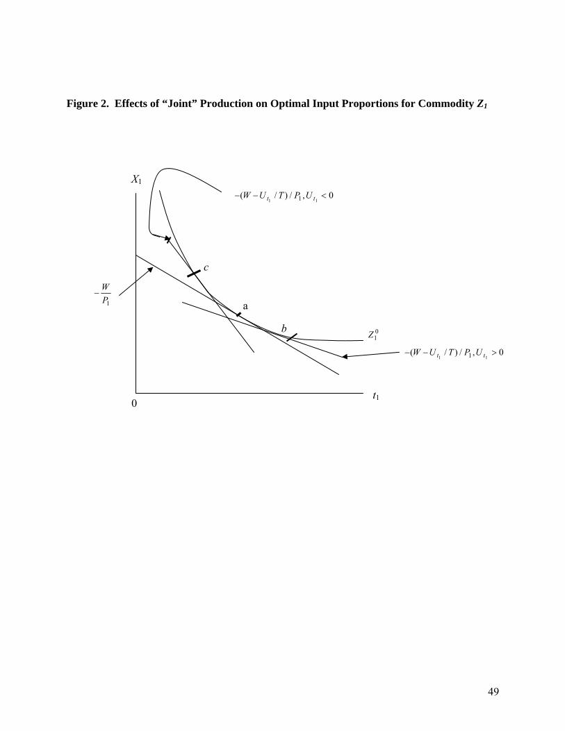
49

Figure 2. Effects of “Joint” Production on Optimal Input Proportions for Commodity Z1

X1

t1

0,/)/(11 1 >−− tt UPTUW

0,/)/(11 1 <−− tt UPTUW

c

a

b 01Z

1PW

−

0

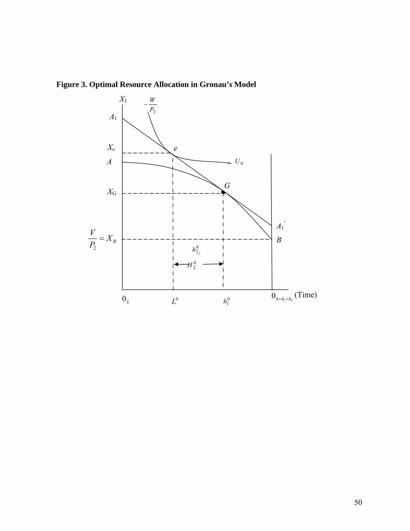
50

Figure 3. Optimal Resource Allocation in Gronau’s Model

210 hhh +=

(Time)

G

A

BXPV

=2

XG

0L 01h

022

h

02H

0U

A1′

B

A1

L0

e

X1

Xe

2PW

−

Figure 4. Average Annual Hours of Unpaid Household Work of Employed and Not Employed Men and Women, 16-64 Years of Age: 1948-1996

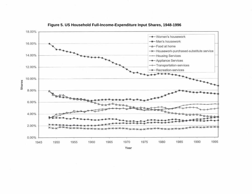
Figure 5. US Household Full-Income-Expenditure Input Shares, 1948-1996

Figure 6. Prices of Inputs for US Household Relative to the Stone Cost of Living Index, 1948-1996

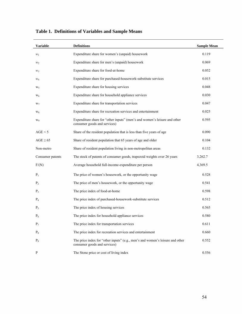
54

Table 1. Definitions of Variables and Sample Means

Variable

Definitions

Sample Mean

w1 Expenditure share for women’s (unpaid) housework

0.119

w2 Expenditure share for men’s (unpaid) housework

0.069

w3 Expenditure share for food-at-home

0.052

w4 Expenditure share for purchased-housework-substitute services

0.015

w5 Expenditure share for housing services

0.048

w6 Expenditure share for household appliance services

0.030

w7 Expenditure share for transportation services

0.047

w8 Expenditure share for recreation services and entertainment

0.025

w9 Expenditure share for “other inputs” (men’s and women’s leisure and other consumer goods and services)

0.595

AGE < 5 Share of the resident population that is less than five years of age

0.090

AGE ≥ 65 Share of resident population that 65 years of age and older

0.104

Non-metro Share of resident population living in non-metropolitan areas

0.132

Consumer patents The stock of patents of consumer goods, trapezoid weights over 26 years

3,262.7

F/(N) Average household full-income-expenditure per person 4,369.5

P1 The price of women’s housework, or the opportunity wage

0.528

P2 The price of men’s housework, or the opportunity wage

0.541

P3 The price index of food-at-home

0.598

P4 The price index of purchased-housework-substitute services

0.512

P5 The price index of housing services

0.565

P6 The price index for household appliance services

0.580

P7 The price index for transportation services

0.611

P8 The price index for recreation services and entertainment

0.660

P9

P

The price index for “other inputs” (e.g., men’s and women’s leisure and other consumer goods and services) The Stone price or cost of living index

0.552 0.556

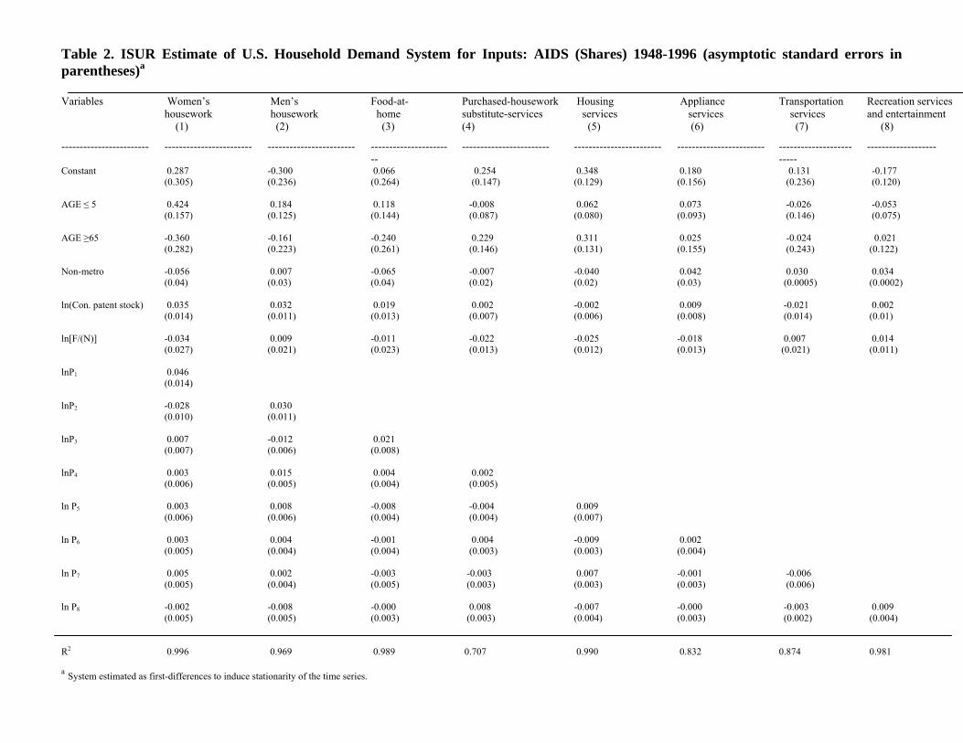
Table 2. ISUR Estimate of U.S. Household Demand System for Inputs: AIDS (Shares) 1948-1996 (asymptotic standard errors in parentheses)a Variables

Women’s housework (1)

Men’s housework (2)

Food-at- home (3)

Purchased-housework substitute-services (4)

Housing services (5)

Appliance services (6)

Transportation services (7)

Recreation services and entertainment (8)

------------------------ ------------------------ ------------------------ -----------------------

------------------------ ------------------------ ------------------------ -------------------------

-------------------

Constant 0.287 (0.305)

-0.300 (0.236)

0.066 (0.264)

0.254 (0.147)

0.348 (0.129)

0.180 (0.156)

0.131 (0.236)

-0.177 (0.120)

AGE ≤ 5 0.424 (0.157)

0.184 (0.125)

0.118 (0.144)

-0.008 (0.087)

0.062 (0.080)

0.073 (0.093)

-0.026 (0.146)

-0.053 (0.075)

AGE ≥65 -0.360 (0.282)

-0.161 (0.223)

-0.240 (0.261)

0.229 (0.146)

0.311 (0.131)

0.025 (0.155)

-0.024 (0.243)

0.021 (0.122)

Non-metro -0.056 (0.04)

0.007 (0.03)

-0.065 (0.04)

-0.007 (0.02)

-0.040 (0.02)

0.042 (0.03)

0.030 (0.0005)

0.034 (0.0002)

ln(Con. patent stock) 0.035 (0.014)

0.032 (0.011)

0.019 (0.013)

0.002 (0.007)

-0.002 (0.006)

0.009 (0.008)

-0.021 (0.014)

0.002 (0.01)

ln[F/(N)] -0.034 (0.027)

0.009 (0.021)

-0.011 (0.023)

-0.022 (0.013)

-0.025 (0.012)

-0.018 (0.013)

0.007 (0.021)

0.014 (0.011)

lnP1 0.046 (0.014)

lnP2 -0.028 (0.010)

0.030 (0.011)

lnP3 0.007 (0.007)

-0.012 (0.006)

0.021 (0.008)

lnP4 0.003 (0.006)

0.015 (0.005)

0.004 (0.004)

0.002 (0.005)

ln P5 0.003 (0.006)

0.008 (0.006)

-0.008 (0.004)

-0.004 (0.004)

0.009 (0.007)

ln P6 0.003 (0.005)

0.004 (0.004)

-0.001 (0.004)

0.004 (0.003)

-0.009 (0.003)

0.002 (0.004)

ln P7 0.005 (0.005)

0.002 (0.004)

-0.003 (0.005)

-0.003 (0.003)

0.007 (0.003)

-0.001 (0.003)

-0.006 (0.006)

ln P8 -0.002 (0.005)

-0.008 (0.005)

-0.000 (0.003)

0.008 (0.003)

-0.007 (0.004)

-0.000 (0.003)

-0.003 (0.002)

0.009 (0.004)

R2

0.996

0.969

0.989

0.707

0.990

0.832

0.874

0.981

a System estimated as first-differences to induce stationarity of the time series.

Table 3. Estimates of Price and Income Elasticities: AIDS Model with Nine Input Groups, US Aggregate Data, 1950-96 (z-values are in parentheses).

_____________________________________________________________________________________________________________________ Prices (j) Income/

__________________________________________________________________ Expenditure Commodity/Input groups (i) 1 2 3 4 5 6 7 8 9 Elasticity

compensated ( e*

ij ) ________________________________________________________________________________________________________________________________ 1) Women’s housework -0.493 -0.164 0.110 0.043 0.070 0.053 0.085 0.007 0.289 0.713 (4.29) (1.99) (1.81) (0.90) (1.29) (1.30) (1.95) (0.15) (1.68) (3.16) 2) Men’s housework -0.283 -0.489 -0.116 0.229 0.166 0.087 0.077 -0.085 0.414 1.136 (1.99) (3.14) (1.35) (3.11) (1.93) (1.45) (1.22) (1.21) (1.73) (3.75) 3) Food-at-home 0.253 -0.154 -0.553 0.098 -0.109 0.002 -0.015 0.016 0.463 0.793 (1.81) (1.35) (3.71) (1.23) (1.50) (0.03) (0.17) (0.24) (1.44) (1.81) 4) Purchased-housework-substitute services 0.330 1.019 0.328 -0.882 -0.184 0.295 -0.139 0.075 -0.841 -0.420 (0.90) (3.11) (1.23) (2.79) (0.77) (1.51) (0.75) (0.36) (1.22) (0.51) 5) Housing services 0.173 0.238 -0.119 -0.060 -0.757 -0.159 -0.093 -0.113 0.888 0.480 (1.29) (1.93) (1.50) (0.77) (5.28) (2.56) (1.71) (1.32) (4.16) (1.99) 6) Household appliance services 0.211 0.202 0.004 0.153 -0.255 -0.887 0.008 0.024 0.541 0.392 (1.30) (1.45) (0.03) (1.51) (2.56) (7.45) (0.08) (0.28) (1.51) (0.88) 7) Transportation services 0.217 0.113 -0.017 -0.046 -0.095 0.005 -1.087 -0.029 0.937 1.151 (1.95) (1.22) (0.17) (0.76) (1.71) (0.08) (8.92) (0.56) (3.37) (2.63) 8) Recreation services and entertainment 0.032 -0.236 0.034 0.047 -0.219 0.029 -0.055 -0.628 0.997 1.579 (0.15) (1.21) (0.24) (0.36) (1.32) (0.28) (0.56) (3.56) (2.64) (3.71) 9) “Other inputs” 0.058 0.048 0.040 -0.022 0.071 0.027 0.074 0.041 -0.338 1.133

(1.68) (1.73) (1.44) (1.22) (4.16) (1.51) (3.37) (2.64) (3.48) (10.08)