Embed Size (px)
Citation preview

Household Leverage and the Recession of 2007 to 2009
Atif Mian
University of Chicago and NBER
Amir Sufi
University of Chicago and NBER
Paper presented at the 10th Jacques Polak Annual Research Conference Hosted by the International Monetary Fund Washington, DC─November 5–6, 2009 The views expressed in this paper are those of the author(s) only, and the presence
of them, or of links to them, on the IMF website does not imply that the IMF, its Executive Board, or its management endorses or shares the views expressed in the paper.
1100TTHH JJAACCQQUUEESS PPOOLLAAKK AANNNNUUAALL RREESSEEAARRCCHH CCOONNFFEERREENNCCEE NNOOVVEEMMBBEERR 55--66,, 22000099
Household Leverage and the Recession of 2007 to 2009
Atif Mian University of Chicago Booth School of Business and NBER
Amir Sufi
University of Chicago Booth School of Business and NBER
October 2009
Abstract
We show that household leverage is an early and powerful predictor of the 2007 to 2009 recession. Counties in the U.S. that experienced a large increase in household leverage from 2002 to 2006 showed a sharp relative decline in durable consumption starting in the third quarter of 2006 – a full year before any significant change in unemployment. Similarly, counties with the highest reliance on credit card borrowing reduced durable consumption by significantly more following the financial crisis of the fall of 2008. Overall, our estimates show that household leverage growth and dependence on credit card borrowing explain a large fraction of the overall consumer default, house price, unemployment, residential investment, and durable consumption patterns during the recession. Our findings suggest that a focus on household finance may help elucidate the sources macroeconomic fluctuations.
* We thank Pierre-Olivier Gourinchas, Ayhan Kose and seminar participants at Chicago Booth, Duke University (Fuqua), Purdue University (Krannert), Harvard Business School, and Wharton for comments. Timothy Dore provided superb research assistance. We are grateful to the National Science Foundation, the Initiative on Global Markets at the University of Chicago Booth School of Business, the Center for Research in Security Prices, and the FMC Corporation for funding. The results or views expressed in this study are those of the authors and do not reflect those of the providers of the data used in this analysis. Mian: (773) 834 8266, [email protected]; Sufi: (773) 702 6148, [email protected]
1
Understanding the sources of deep recessions is the holy grail of macroeconomics. The
most recent recession has produced a sharp increase in unemployment and a deep decline in
GDP (Figure I, top two panels). What factors explain the current economic downturn? While a
number of reasonable hypotheses have been put forward, an empirically relevant theory must
quantitatively explain four facts that collectively define the recession: the sharp rise in household
defaults, the fall in house prices, the drop in consumption (especially durables), and the rise in
unemployment.
In this study, we focus on the rapid growth in household leverage in the years before the
recession, and we find that household leverage growth performs remarkably well in explaining
these four facts. The bottom panel of Figure 1 shows the unprecedented increase in the U.S.
household debt to income ratio during the years prior to the recession. In 2007, the household
debt to GDP ratio reached its highest level since the onset of the Great Depression. Our main
results are consistent with the view that the dramatic increase in household leverage from 2000
to 2007 was a primary driver of the recession of 2007 to 2009.
The aggregate U.S. evidence highlights the importance of household leverage. The initial
indicators of economic difficulty were a rise in household default rates and a decline in house
prices, both of which reflected an overstretched household sector. These trends began as early as
the second quarter of 2006, a full five quarters before the initial increase in the unemployment
rate. Not surprisingly, the components of GDP that initially declined in 2007 and early 2008
were fixed residential investment and durable consumption—the two components that most
heavily rely on the willingness of households to obtain additional debt financing.
While aggregate patterns hint at the importance of household leverage in precipitating the
recession, it is difficult to reach definitive conclusions on the link between household leverage
2
and the economy based on aggregate data alone. For example, it is possible that the decline in
house prices and the increase in defaults in 2006 reflected an anticipation of future
unemployment. Or perhaps the household-leverage component of the recession, while occurring
early in the downturn, is far less important than the credit crisis of September and October of
2008. More generally, the linkages across the economy make it difficult to conclude based on
aggregate evidence alone what factors contributed to the severe recession of 2007 to 2009.
To overcome these difficulties, we focus on cross-sectional variation across U.S. counties
in the severity of the recession. There is a large degree of such variation. For example, Saint
Lucie County in Florida experienced an increase in the unemployment rate of 6.6% from 2006 to
2008. In contrast, Harris County in Texas, where Houston is located, had a rise of only 1.2% in
the unemployment rate. Our empirical methodology examines patterns across U.S. counties to
explore why some counties have experienced a much more severe recession than others.
We sort counties according to the increase in the household debt to income ratio from
2002 to 2006, and we refer to counties with large (small) increases in leverage during this period
as high (low) leverage growth counties. We find that the recession both began earlier and became
more severe in high leverage growth counties relative to low leverage growth counties. The top
10% leverage growth counties experienced an increase in the household default rate of 12
percentage points and a decline in house prices of 40% from the second quarter of 2006 through
the second quarter of 2009. In contrast, the bottom 10% leverage growth counties experienced a
modest increase of 3 percentage points in the default rate and a 10% increase in house prices. In
other words, household leverage growth from 2002 to 2006 strongly predicted subsequent
housing and consumer credit difficulties across U.S. counties.
3
Auto sales and new housing building permits reveal a similar pattern. By the third quarter
of 2008, auto sales in the top 10% leverage growth counties declined by almost 40% relative to
2005. In contrast, auto sales in the bottom 10% leverage growth counties were actually up almost
20%. From 2005 to 2008, new housing building permits declined by almost 150% in high
leverage growth counties while declining only 50% in low leverage growth counties. The
dramatic differential shows the importance of household leverage in the sharp decline in durable
consumption and residential investment that precipitated the recession. To the best of our
knowledge, we are the first to examine durable consumption and residential investment patterns
across U.S. counties during a recession, and the first to show the importance of household
leverage in explaining why some counties experience much sharper declines than others.
The final measure of economic activity we examine is the unemployment rate. Similar to
the pattern in auto sales, the unemployment rate increased in high leverage growth counties
much earlier than low leverage counties. From the fourth quarter of 2005 to the third quarter of
2008, the unemployment rate climbed 2.5 percentage points in the top 10% leverage growth
counties; in contrast, the bottom 10% leverage growth counties experienced no change in
unemployment.
The evidence suggests that both the timing and the severity of the recession were closely
related to the increase in household leverage from 2002 to 2006. Counties that experienced a
large increase in their debt to income ratio before the onset of the downturn were precisely the
counties that experienced the sharpest decline in durable consumption and the largest increase in
unemployment. We also show that the correlation between leverage growth and the severity of
the recession is robust to county-level control variables for demographics, cyclicality, and
industrial composition.
4
While counties with low leverage largely escaped the recession up to the third quarter of
2008, auto sales drop and unemployment skyrocket in both high and low leverage growth
counties from the fourth quarter of 2008 through the second quarter of 2009. In other words, the
growth household leverage from 2002 to 2006 does not predict the severity of the downturn
during the last three quarters of the recession.
In the last section of our analysis, we examine what factors other than household leverage
growth from 2002 to 2006 explain why the severity of the recession accelerated from the fourth
quarter of 2008 to the second quarter of 2009. We find that the severity of the downturn in these
three quarters can be explained by an alternative measure of household leverage: household
exposure to short term credit, as measured by the credit card utilization rate as of 2006. High
credit card utilization rate counties experience a sharper drop in auto sales from the fourth
quarter of 2008 through the second quarter of 2009. This coincides with a sharp reduction in
credit card availability that occurs simultaneously with the financial crisis in September and
October of 2008.
Our findings suggest that households faced a one-two punch during the recession. From
the fourth quarter of 2006 to the third quarter of 2008, an over-levered household sector facing
mounting defaults and falling house prices pulled back on durable consumption and experienced
higher unemployment rates. From the fourth quarter of 2008 onwards, credit-card dependent
consumers reduced consumption as credit card availability was cut dramatically.
In terms of magnitudes, our two household leverage based factors work remarkably well
in explaining many features of the recession. Growth in household leverage from 2002 to 2006
and household dependence on credit card borrowing as of 2006 are quantitatively sufficient to
explain the entire rise in household defaults, the drop in house prices, and the drop in auto sales.
5
Our factors also explain about a fifth of the overall rise in unemployment. The reduced
explanatory power for unemployment is a natural outcome of the fact that goods consumed in
one location are often produced in different locations, therefore naturally lowering the
correlation between local consumption and production shocks.1
Overall, our findings support the hypothesis that household balance sheets are a crucial
component of explaining macroeconomic fluctuations. The idea that household debt instigates
and exacerbates economic downturns goes back to Fisher (1933), and is also related to research
by Mishkin (1978), King (1994), and Leamer (2007, 2009). In particular, Leamer (2007, 2009)
points out that eight of the past ten recessions were preceded by substantial problems in housing
and consumer durables. Our paper provides the first micro-level cross-sectional evidence based
on the 2007 to 2009 recession of the link between household balance sheets and an economic
downturn.2
We believe more research is needed to determine whether household leverage was a
catalyst of the recession or an amplification of other variables, such as technology or monetary
shocks. However, any argument in favor of an alternative factor driving the current recession
must be consistent with the strong power of household leverage in predicting economic
outcomes in the cross-section of U.S. counties.
The rest of the study proceeds as follows. In the next section, we provide aggregate
evidence consistent with the importance of household leverage in the current recession. In
Section 2, we describe the county-level data and provide summary statistics. In Section 3, we
focus on the relation between leverage growth from 2002 to 2006 and economic outcomes from
1 For example, reduced recreational vehicle (RV) sales in Los Angeles County due to household leverage may lead to a sharp increase in unemployment in Elkhart County, Indiana, even though Elkhart County has low household leverage. 2 Another recent paper on the topic is Glick and Lansing (2009).
6
2006 to 2009. Section 4 explores alternative hypotheses and shows how credit card-reliant
borrowers responded to the financial crisis of the fall of 2008. Section 5 presents our magnitude
estimation, and Section 6 concludes.
Section 1. Household Leverage and the Real Economy
A. The Origins of Household Leverage
What factors led to the dramatic expansion in household leverage from 2001 to 2007?
This is the central question of two of our previous studies. In Mian and Sufi (2009a), we argue
that the advent of subprime mortgage securitization represented a credit supply shock that
provided new home purchase financing for a segment of the population that traditionally was
unable to obtain mortgages. We are agnostic on the source of the credit supply shock—it is likely
that government programs (Leonnig (2008)), moral hazard on behalf of originators and servicers
of securitization pools (Keys, Mukherjee, Seru, and Vig (2010), and the enormous capital
inflows into the United States (Obstfeld and Rogoff (2009)) all played some role. We present
evidence that the credit supply shock led to an increase in house prices, which led to an
important collateral feedback effect: once collateral values increased, lenders were willing to
lend even more to households (Kiyotaki and Moore (1997)).
In Mian and Sufi (2009b), we focus on existing homeowners who owned their homes
before the credit supply shock. We find that existing homeowners responded to house price
growth by borrowing heavily against the increase in the value of their home equity. We find that
homeowners borrowed 25 to 30 cents on every dollar of home value appreciation, and that this
home equity-based borrowing channel accounts for a substantial fraction of the increase in
homeowner debt from 2002 to 2006.
7
To summarize, two related factors are responsible for the rise in household leverage
between 2001 and 2007. First, an expansion in the supply of credit pulled new buyers into the
housing market, pushing house prices up in the process. Second, the increase in house prices and
low interest rates enticed existing homeowners to extract cash from their home equity. Perhaps
as important as these two factors is what is missing: the cross-sectional analyses in our two
previous papers are inconsistent with the view that a positive productivity or technology shock
was responsible for the sharp rise in household leverage.
B. Household Leverage and the Real Economy
This historic rise in household leverage proved to be unsustainable. The top panel in
Figure 2 shows that beginning in the second quarter of 2006, default rates began to rise and
house prices began to fall. As early as the second quarter of 2007—two months before the
beginning of the current recession—default rates were already above the levels they had reached
in the 2001 recession. By the second quarter of 2009, the default rate neared 10%, which is twice
as high as any point since 1991. Total delinquent debt as of the second quarter of 2009 was $1.7
trillion.
The painful process of household de-leveraging began in the second quarter of 2008
(lower panel). Households cut back on consumption as the personal savings rate reached 5.2% in
the second quarter of 2009 - the highest it has been in over a decade. As early as the fourth
quarter of 2007, debt growth began to moderate. From the fourth quarter of 2008 to the second
quarter of 2009, total household debt declined for three straight quarters—something that had not
previously occurred in the past 60 years for which quarterly data are available.
Why did mortgage defaults begin to rise and house prices begin to fall in the middle of
2006? This question is beyond the scope of our analysis, but we offer three potential reasons.
8
First, rising interest rates likely played a role in reducing house prices by lowering the relative
advantage of homeownership (Mayer and Hubbard (2008)). Second, lending standards on
mortgages deteriorated to such a degree that mortgages originated in 2006 experienced
shockingly high default rates almost immediately after origination (Demyanyk and Van Hemert
(2008)). Third, even small increases in default rates may have shut down securitization markets,
leading to an amplification effect on default rates as households were unable to refinance.
One thing is certain: the rise in mortgage defaults preceded the rise in unemployment, not
vice versa. Figure 3 shows that the increase in default rates started five quarters before any rise in
unemployment. This sequence of changes casts doubt on the view that initial mortgage defaults
reflected difficulties in the labor market. Instead it was increased difficulty in repayment of
household debt that precipitated the downturn.
Figure 4 shows that household financial stress immediately translated into declines in real
activity. Starting in the first quarter of 2006, residential fixed investment growth began to
plummet. By the fourth quarter of 2007, residential fixed investment had declined almost 50%
from its 2005 level. In contrast, non-residential fixed investment showed robust growth until the
third quarter of 2008. The middle panel of Figure 4 shows a similar pattern for durable
consumption, which leveled off in 2007 before experiencing sharp declines through 2008. Non-
durable and service consumption remained strong until the end of 2008.
The bottom panel of Figure 4 shows monthly retail sales; as it shows, the drop in durable
consumption (motor vehicles, and furniture and appliances) began very early in the recession.
The drop in auto sales was particularly large—from the fourth quarter of 2007 to the fourth
quarter of 2008, auto sales dropped by 30%. The drop in non-durable consumption both began
later and was far less severe.
9
The aggregate evidence is consistent with the view that the rise in household leverage
was a main catalyst of the 2007 to 2009 U.S. recession. Deterioration in household balance
sheets began as early as 2006 and was followed immediately by a sharp drop in residential fixed
investment and durable consumption. These latter two components are the most reliant on
households’ willingness to access additional debt finance, so it is not surprising that they moved
first. By the end of 2008, the household de-leveraging process was in full swing.
In the next section, we begin our analysis of the cross-section of U.S. counties to provide
further evidence on the view that household leverage is a powerful predictor of economic
outcomes during the 2007 to 2009 recession.
Section 2. County-Level Data and Summary Statistics
We build the county-level data set from a variety of sources. Information on household
debt, default rates, and credit scores comes from Equifax zip code level aggregates. Data on
house prices come from the FHFA MSA level house price indices, which are subsequently
matched to counties. Zip code level income information is available from the IRS, and zip code
level demographics are from the 2000 Decennial Census. More information on these data sets is
available in the appendix of Mian and Sufi (2009a). The zip code level data in Equifax are
aggregated to the county level by weighting each zip code by the fraction of all consumers with a
credit report in the county living in the zip code. The IRS and Census zip code level data are
aggregated to the county level using the number of households in the 2000 census as weights.
There are four new county-level data sets that we do not employ in our previous studies.
The first includes auto sales data from R.L. Polk. Polk is an automotive intelligence company
that provides detailed auto sales data to a variety of customers. The data are collected by
10
examining new vehicle registrations at the county level. The data are available from 2004 to
2009 at a quarterly frequency, and they cover every county in the United States.3 County-level
unemployment data are from the Bureau of Labor Statistics, who provide quarterly
unemployment rate data for all U.S. counties. We use county business patterns data from the
Census Bureau to construct industry composition of employment for each county. The business
patterns data records payroll and employment data by industry for each county and is available
with a three year lag. New housing permits also come from the Census Bureau.4
While there are 3,138 counties in the U.S., we restrict our attention to the top 450
counties in the U.S. by population. These are counties with at least 50,000 resident households,
which cover 70% of the U.S. population and 82% of the aggregate debt outstanding as of the end
of 2005. Since our focus is on county-level analysis in this paper, we drop the very small
counties that add significant measurement error. All of our results are unchanged if we include
small counties, but give them their appropriate statistical weight by weighing by county
population.
Every state and the District of Columbia are represented by the counties in our sample,
with the exception of Wyoming. To get a sense of the counties included, we list in the Appendix
Table every fifth county in our final sample, where the counties are sorted inversely according to
the change in the debt to income ratio from 2002 to 2006 (i.e., counties with the largest increase
in the debt to income ratio are listed first).
Table 1 presents summary statistics for the final sample of 450 counties. The key variable
of interest in our study is the increase in the debt to income ratio across counties from 2002 to
3 These data are available for purchase from R.L. Polk. For pricing information and purchase, please contact Robert Sacka at [email protected], and mention the county-level quarterly auto sales data used in this study. 4County-level census data are available at: http://www2.census.gov/prod2/statcomp/usac/excel/
11
2006. The average debt to income increase across counties from 2002 to 2006 was 0.8. The
average debt to income ratio as of 2001 was 2.2 with a standard deviation of 0.5, which implies
that the increase from 2002 to 2006 was more than one full standard deviation of the 2001 level.
The average increase in the default rates of counties from the fourth quarter of 2006 to
the second quarter of 2009 was 0.043, which is almost three times as large as one standard
deviation of the 2006 level. House prices collapsed from 2006 to 2009, with the average decline
across counties in our sample of 14%. House price data are only available for 123 counties; this
reflects the limits of the coverage of MSAs by FHFA.
Table 1 also shows that auto sales plummeted by an average of 32% from the fourth
quarter of 2006 to the second quarter of 2009. Over the same time period, the unemployment rate
increased by an average of 5.4 percentage points, which is more than 4 times a standard
deviation of the 2006 level. Table 1 also includes information on Census demographics and
county business patterns across the 450 counties in our sample.
Section 3. Household Leverage and the Real Economy: County-Level Analysis
In this section, we examine how household leverage growth in a given county from 2002
to 2006 affected the timing and severity of the recession in the county from 2006 to 2009. As we
show, counties with the largest increases in household leverage experienced the earliest and most
severe downturns in economic activity.
A. Methodology
There are five county-level economic outcomes we evaluate: mortgage default rates,
house price growth, auto sales, new housing building permits, and unemployment. The goal of
our methodology is to see how the increase in leverage from 2002 to 2006 in a given county
12
affects these county-level outcomes during the recession. We first split the sample into high and
low leverage growth counties. High leverage growth counties are counties in the top 10% of the
distribution of the increase in the debt to income ratio from 2002 to 2006. For example, Merced
County in California experienced an increase in its aggregate debt to income of 2.3 from 2002 to
2006. Low leverage growth counties are counties in the bottom 10% of the same distribution. For
example, Tarrant County in Texas experienced almost no increase in its debt to income ratio
from 2002 to 2006. Once we split the sample into high and low leverage growth counties, we
present figures that plot each economic outcome from the fourth quarter of 2004 to the end of the
sample. This technique shows both the timing and severity of the downturn in high versus low
leverage growth counties.
Our second approach is to present figures that contain the county-level scatter plot of the
change in each economic outcome during the recession against the rise in leverage that preceded
the recession. For example, for each county, we plot the increase in the unemployment rate from
the fourth quarter of 2006 to second quarter of 2009 against the rise in household leverage from
the fourth quarter of 2002 to the fourth quarter of 2006.
Third, for each outcome, we present a series of first difference regressions with county-
level control variables. The following equation represents the general form of the first difference
specifications:
06 4_09 2 02 4_06 4 Γ (1)
where EconomicOutcome06q4_09q2 represents the change in the outcome (house prices, default
rates, unemployment, and auto sales) for county i from the fourth quarter of 2006 to the second
quarter of 2009, LeverageGrowth02q4_06q4 represents the increase in the debt to income ratio
in county i from the fourth quarter of 2002 to the fourth quarter of 2006, and ControlVariables is
a set of cyclicality, demographic, and industrial composition measures for county i. In estimating
13
specification (1), we weight by the total number of households in the county as of 2000 to
account for the fact that variables measured over smaller populations have larger variance. We
also report unweighted regression results in all our tables. Standard errors in all specification are
clustered at the state level.
In most of our empirical tests, we take the variation across counties in leverage growth
from 2002 to 2006 as given. In other words, we do not attempt to discern why some counties
experienced sharper increases in household leverage than others. This issue is addressed in our
previous studies. In both Mian and Sufi (2009a) and Mian and Sufi (2009b), we show that an
aggregate credit supply shock beginning in 2002 shifted the demand for housing across the
country. The degree to which house prices increased in respond to this housing demand shock
depended crucially on the slope of the housing supply curve. In counties with relatively elastic
housing supply, house prices were relatively steady as home-builders responded to the demand
shock by constructing more homes. In counties with relatively inelastic housing supply, house
prices increased given the difficulty in constructing more homes to meet new demand.
As a corollary, as counties with inelastic housing supply experienced sharper increases in
house prices, existing homeowners aggressively borrowed against the value of their homes
(Mian and Sufi (2009b)) and new homeowners were forced to take out larger mortgages to buy
more expensive homes (Mian and Sufi (2009a)). The primary measure of housing supply
elasticity we use in the previous studies comes from Saiz (2008), who constructs his measure
based on geographical and topographical constraints on house construction.
The impact of housing supply elasticity on leverage growth is quite strong: a county level
regression of the increase in the debt to income ratio from 2002 to 2006 on the Saiz (2008)
measure of housing supply inelasticity shows a strongly positive correlation with an R2 of almost
14
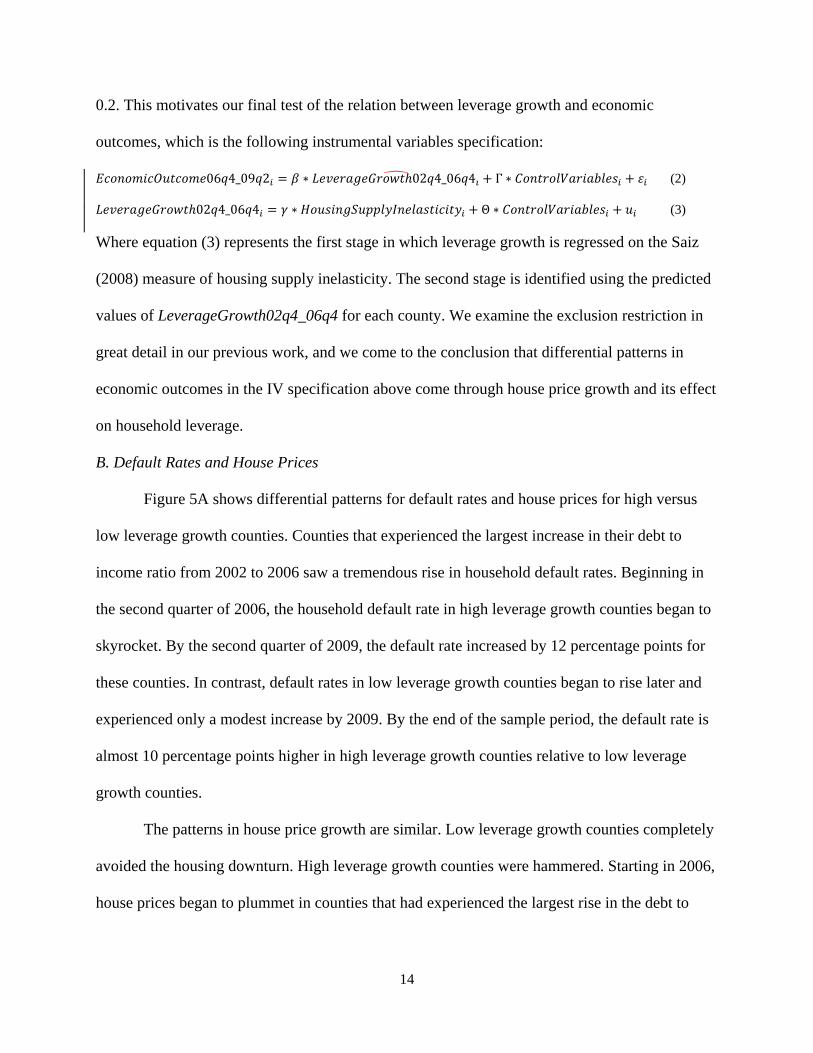
0.2. This motivates our final test of the relation between leverage growth and economic
outcomes, which is the following instrumental variables specification:
06 4_09 2 02 4_06 4 Γ (2)
02 4_06 4 Θ (3)
Where equation (3) represents the first stage in which leverage growth is regressed on the Saiz
(2008) measure of housing supply inelasticity. The second stage is identified using the predicted
values of LeverageGrowth02q4_06q4 for each county. We examine the exclusion restriction in
great detail in our previous work, and we come to the conclusion that differential patterns in
economic outcomes in the IV specification above come through house price growth and its effect
on household leverage.
B. Default Rates and House Prices
Figure 5A shows differential patterns for default rates and house prices for high versus
low leverage growth counties. Counties that experienced the largest increase in their debt to
income ratio from 2002 to 2006 saw a tremendous rise in household default rates. Beginning in
the second quarter of 2006, the household default rate in high leverage growth counties began to
skyrocket. By the second quarter of 2009, the default rate increased by 12 percentage points for
these counties. In contrast, default rates in low leverage growth counties began to rise later and
experienced only a modest increase by 2009. By the end of the sample period, the default rate is
almost 10 percentage points higher in high leverage growth counties relative to low leverage
growth counties.
The patterns in house price growth are similar. Low leverage growth counties completely
avoided the housing downturn. High leverage growth counties were hammered. Starting in 2006,
house prices began to plummet in counties that had experienced the largest rise in the debt to
15
income ratio from 2002 to 2006. From 2005 to the second quarter of 2009, house prices dropped
a stunning 40% in high leverage growth counties.
Figure 5B shows the scatter plots for the change in these two outcome variables from
2006 to 2009 against the increase in household leverage from 2002 to 2006. As they show, the
increase in household leverage before the recession in a given county strongly predicts the
severity of the subsequent default and housing crisis within the same county. The magnitudes are
very large: the regression line implies that a one standard deviation increase in leverage growth
from 2002 to 2006 leads to a 2/3 standard deviation increase in subsequent default rates and a 2/3
standard deviation decline in subsequent house price growth.
Tables 2 and 3 present the first difference regression analogs to the scatter plots, and they
show that the correlations in Figure 5B are robust to the inclusion of control variables. In column
1 of Table 2, the change in the debt to income ratio from 2002 to 2006 is strongly correlated with
the increase in default rates from 2006 to 2009. This single variable gives an R2 of 0.45, which is
extremely high for a first-difference cross-section regression. Column 2 presents the coefficient
estimate after weighting the observations by the number of households in the county as of 2000.
In columns 3 and 4, we include a variety of control variables that increase the adjusted R2
substantially. The inclusion of control variables actually increases the size of the coefficient on
leverage growth. Column 5 presents the IV estimate where the change in the debt to income ratio
is instrumented using the Saiz (2008) measure of housing supply inelasticity. The IV estimate is
considerably larger than the OLS estimate, which may be may be driven by two factors. First, the
IV could be correcting for some measurement error in leverage growth. Second, to the extent
some of the increase in leverage is driven by real permanent income shocks, it would tend to
reduce ex-post differences between high and low leverage growth counties. For example, if high
16
leverage growth were driven by an accurate expectation of higher income growth in future, then
leverage growth will not predict high default rates. Since our housing supply elasticity
instrument is uncorrelated with such permanent income shock differences (see Mian and Sufi
2009b for evidence), the IV specification corrects for the endogeneity problem.
The coefficient in column 1 of Table 3 shows the strong negative correlation between
leverage growth from 2002 to 2006 and subsequent house price growth. The univariate
specification yields an R2 of 0.62. As before, the inclusion of control variables improves the fit
of the regression, but has almost no effect on the relation between leverage growth and house
price growth. As with default rates, the IV estimate is larger than the OLS estimate, although the
coefficient is not estimated precisely.
C. Auto Sales, New Housing Permits, and Unemployment Rates
In Figure 6A, we plot the differential patterns in auto sales, new housing building
permits, and unemployment rates for high versus low leverage growth counties. Counties that
experienced the largest increase in their debt to income ratio from 2002 to 2006 saw a severe
contraction in auto sales very early in the downturn. By the first quarter of 2008, auto sales
dropped 20% relative to their 2005 level in high leverage growth counties. In contrast, auto sales
were actually up in low leverage growth counties in the first quarter of 2008. In the third quarter
of 2008, auto sales dropped in both high and low leverage growth counties, but the drop in high
leverage growth counties was much more severe. Interestingly, all counties saw auto sales
plummet in the fourth quarter of 2008 and the first quarter of 2009. We return to this latter fact in
Section 4.
The middle panel of Figure 6A plots the differential patterns for new housing permits.
High leverage growth counties experienced a much earlier and more severe downturn in new
17
housing permit growth. At the end of 2007, new housing permits declined in counties
experiencing a large increase in leverage from 2002 to 2006 by 75%. The decline in counties
experiencing no increase in leverage from 2002 to 2006 was only 20%. The differential only
increased from 2007 to 2008.
Perhaps the most important measure of recession severity is the unemployment rate. The
right panel of Figure 6A shows that the rise in unemployment began much earlier in high versus
low leverage growth counties, and the subsequent increase in unemployment was much more
severe. As early as the middle of 2007, the unemployment rate had increased more sharply in
counties that had experienced the largest increase in their debt to income ratios from 2002 to
2006.
While the unemployment rate is relatively constant in low leverage growth counties
through the third quarter of 2008, it increases sharply from the third quarter of 2008 to the
second quarter of 2009. This is similar to the pattern in auto sales. In other words, while
household leverage strongly predicts auto sales and unemployment through the third quarter of
2008, all counties experience dramatic declines in auto sales and dramatic increases in
unemployment during the last part of the recession.
Figure 6B presents the scatter plots of the relation between leverage growth from 2002 to
2006 and the change in auto sales, new housing permits, and unemployment from 2006 to 2009.
The plots show a negative correlation between leverage growth and subsequent auto sales growth
and leverage growth and subsequent new housing permit growth. The right panel shows a
positive correlation between leverage growth and subsequent increases in unemployment. The
scatter plots show a significant amount of unexplained variation, which we examine in the next
section.
18
Table 4 presents coefficients from the first difference specification of auto sales growth
from the fourth quarter of 2006 to the second quarter of 2009 regressed on leverage growth from
2002 to 2006. The coefficient estimate in column 2 implies that a one standard deviation increase
in leverage growth from 2002 to 2006 in a county was associated with a ½ standard deviation
decrease in auto sales from 2006 to 2009. The inclusion of control variables reduces the
magnitude slightly, but the effect is still large and statistically significant. The IV specification in
column 5 yields a coefficient estimate that is substantially larger, but less precise.
Table 5 replicates the specifications with the growth in new housing building permits
from 2006 to 2008 as the left hand side variable. The coefficient in column 2 implies that a one
standard deviation increase in leverage growth from 2002 to 2006 leads to a 1/3 standard
deviation decrease in new housing permit growth from 2006 to 2008. The inclusion of control
variables does not affect the estimate. The IV specification produces a larger coefficient, but it is
measured less precisely.
The results on new housing building permits raise a possible “real estate construction”
channel through which household leverage affects real economic activity: the housing boom in
high leverage growth counties led to higher employment in real estate construction from 2002 to
2006, and the resulting downturn is a natural response as this sector shrinks. The coefficient
estimate in column 6 disputes this hypothesis. The estimate implies that high leverage growth
counties experienced less residential housing construction during the housing boom than low
leverage growth counties. This is consistent with our previous research that shows that a credit-
induced housing demand shock led to more building in elastic counties (Mian and Sufi (2009b)).
In addition, the employment share in construction and real estate as of the end of 2006 is
19
included as a control variable for all economic outcomes, and this control variable does not affect
the estimated coefficient on leverage growth in any specification.
Table 6 presents coefficients from the first difference specification of the unemployment
rate change from 2006 to 2009 regressed on leverage growth from 2002 to 2006. The coefficient
estimate in column 2 implies that a one standard deviation increase in leverage growth from
2002 to 2006 led to a 1/3 standard deviation increase in the unemployment rate during the
recession. The inclusion of control variables has almost no effect on the magnitude. The IV
estimate is even larger than the OLS estimate.
Taken together, these results demonstrate that one of the most powerful determinants of
the severity and timing of the economic downturn across counties is the county’s expansion in
household leverage from 2002 to 2006. Counties which had experienced the largest increase in
their household debt to income ratios were precisely the counties that saw auto sales plummet
and unemployment rates increase the most. The cross-sectional patterns are consistent with the
view that household leverage was a primary driver of the recession of 2007 to 2009.
Section 4. The Credit Crisis and the Deepening of the Recession
Household leverage growth from 2002 to 2006 explains a very large fraction of the
decline in economic activity from the second quarter of 2006 to the third quarter of 2008.
Counties with modest increases in debt to income ratios from 2002 to 2006 experience almost no
decline in auto sales or increase in unemployment during the early part of the recession.
However, as Figure 6A above shows, both high and low leverage growth counties experience a
dramatic decline in auto sales and a dramatic increase in unemployment from the third quarter of
20
2008 to the second quarter of 2009. In this section, we explore the potential role of the financial
crisis and consumer reliance on credit cards in explaining these patterns.
A. Credit card utilization rates
Figure 7 presents evidence on the evolution of credit card and home equity patterns from
2005 through 2009. Availability under credit lines is a useful measure of credit supply because it
allows us to distinguish supply from credit demand (see Gross and Souleles (2002)). As the top
left panel shows, the supply of credit card availability increased dramatically during the early
part of the recession from the fourth quarter of 2006 to the third quarter of 2008. In other words,
while home equity and mortgage credit markets became significantly tighter in the early part of
the recession, credit card availability was expanding.
As the middle left panel shows, high leverage growth counties took advantage of these
increased limits by borrowing heavily on credit cards during the early part of the recession.
Recall that these same counties experienced a sharp increase in defaults and unemployment and a
sharp decrease in house price growth, residential investment, and auto sales during this same
time period. The sharp relative growth in credit card debt from the fourth quarter of 2007 to the
third quarter of 2008 for high leverage growth counties was either a last attempt to avoid
defaults, or a final draw down on credit cards before inevitable bankruptcy.
As the top left panel shows, the financial crisis in the fall of 2008 led to a sharp reversal
in credit card availability. All counties faced a dramatic reduction in credit card availability,
which is consistent with a large negative aggregate credit supply shock.
As shown in Figure 6A above, both high and low leverage growth counties experienced a
sharp decline in auto sales and a sharp increase in unemployment after the third quarter of 2008.
Can the large negative consumer credit supply shock shown in Figure 7 explain this pattern? To
21
answer this question, we sort counties based on credit card utilization rates as of the fourth
quarter of 2006. Counties with high credit card utilization rates are assumed to be more reliant on
short-term unsecured consumer credit.5
The top panel of Figure 8 presents the correlation between the credit card utilization rate
as of 2006 and the decline in auto sales from the third quarter of 2008 to the second quarter of
2009. There appears to be a negative correlation, although there is a substantial amount of noise.
The bottom panel examines the unemployment rate increase from the third quarter of 2008 to the
second quarter of 2009. There is a very weak positive correlation between credit card utilization
and the subsequent increase in unemployment.
Table 7 presents results using the credit card utilization rate to explain changes in
economic outcomes during the recession. As column 1 of Table 7 shows, the credit card
utilization rate does not add much explanatory power for auto sales growth from the fourth
quarter of 2006 to the third quarter of 2008. In other words, our initial measure of household
leverage appears to be the dominant force early in the recession. In column 2, we examine auto
sales growth for the entire recession; the credit card utilization rate as of 2006 strongly predicts
the decline in auto sales when we examine the entire recession. The magnitude of the coefficient
implies that a one standard deviation increase in credit card utilization rates as of 2006 leads to a
1/3 standard deviation decrease in auto sales. Household leverage growth from 2002 to 2006
continues to strongly predict the decline in auto sales during the recession. Column 3 includes
control variables; the magnitude of the credit card utilization rate declines, but it remains
negative and statistically significant at the 10% level.
5 The correlation across counties between the increase in the debt to income ratio from 2002 to 2006 and the credit card utilization rate as of the fourth quarter of 2006 is statistically significantly negatively correlated. As a result, we are able to separately test the household leverage growth channel from the credit card reliant-consumer channel.
22
The results in columns 2 and 3 suggest two channels through which household finance
affected durable consumption during the recession. From the fourth quarter of 2006 through the
third quarter of 2008, the dramatic increase in household leverage from 2002 to 2006 led to a
significant reduction in auto sales. Following the credit crisis of the fall of 2008, consumers
normally reliant on credit card availability also pulled back on auto purchases.
In columns 4 through 6, we examine whether credit card utilization rates as of 2006
predict the drop in housing permits or the increase in unemployment. Unlike the evidence on
auto sales, we find little evidence of that credit card utilization rates affect housing construction
or unemployment. In other words, there is a large fraction of unexplained variation in housing
permit growth and unemployment growth, especially after the third quarter of 2008.
B. Alternative channels
In this section, we consider whether factors other than household leverage can explain the
severity of the recession. It is important to emphasize that alternative channels must be able to
explain the cross-sectional patterns we observe.
Whenever a financial crisis occurs simultaneously with a severe recession, there is a
possibility that financial market difficulties have an accelerator effect through business credit
availability and investment (Bernanke and Gertler (1989)). Indeed, the results in the previous
subsection suggest a financial accelerator effect through consumer credit supply. However, one
potential argument against our household leverage channel is a local financial accelerator effect:
household defaults in a given county led to difficulties in the local banking sector which in turn
led to a contraction of business credit. The channel was not households cutting back in the face
of enormous debt burdens and reduced credit availability; instead, financial difficulties in the
local banking sector led to the economic downturn.
23
We examine the local financial accelerator hypothesis in Table 8.6 In columns 1 through
3, we isolate the sample to 52 counties that have banks in the county with less than 10% of their
total deposit base in the county. In other words, these counties have almost exclusively national
banks that are unlikely to have large exposure to the household defaults within the county.
Among these national bank counties, we see the exact same relation between the increase in
household leverage from 2002 to 2006 and economic outcomes from 2006 to 2009. It is difficult
to argue that local banking markets are driving the effect in these counties, given that the banks
are major national players.
In columns 4 through 6, we include explicit control variables for charge-offs and net
income for the banks that have branches in the county. The inclusion of such control variables
does not change the coefficient estimates on leverage growth from 2002 to 2006. These results
are inconsistent with the hypothesis that the effect of household leverage on county-level
outcomes is due to a local financial accelerator operating through the business sector.
More generally, a common argument for the severity of the recession of 2007 to 2009 is
an aggregate contraction of credit to businesses. We are skeptical of this view for a number of
reasons. First, non-residential business investment was the last main component of GDP to move
in the cycle. As Figure 4 above shows, investment in equipment in software did not register a
major decline until the fourth quarter of 2008, and the reduction in investment in structures did
not begin until the first quarter of 2009. While the drop in investment in the last part of the
recession may have been due to harsh credit conditions, it is just as likely that businesses cut
investment in response to the dramatic reduction in consumption.
6 Deposit data by county for each bank is constructed using the FDIC Summary of Deposit data. Data on charge-offs and net income is from Call Report data.

24
Second, businesses were in a much healthier financial situation than consumers as of the
third quarter of 2008 when the credit crisis began. Indeed, the corporate debt to income ratio
increased only moderately leading up to the recession (Mian and Sufi (2009b)). A large body of
research documents how businesses used large revolving credit facilities extended during the
credit boom to mitigate the impact of the credit crunch (Ivashina and Scharfstein (2009), Gao
and Yun (2009), Chari, Christiano, and Kehoe (2008)). Survey evidence also suggests that there
was absolutely no evidence of a credit crunch to small businesses through September 2008
(Dunkelburg (2008)).
Third, while consumer defaults have skyrocketed above any level in recent history, direct
measures of corporate distress are still relatively low compared to the 2001 recession. Figure 9
shows the fraction of public firms that are in violation of a financial covenant in any debt
agreement.7 For the 2008 fiscal year (which covers firms filing their 10-K at any point from July
2008 to June 2009), the fraction of firms that violated a financial covenant is still much lower
than during the recession of 2001. According to Standard & Poor’s, the corporate default rate for
speculative-grade firms was 12% at the beginning of 2009, which is significantly below the
corporate default rate of almost 20% registered during the 2001 recession.8 Both covenant
violation and default rate patterns suggest that firms faced less distress than they did in the
relatively mild recession of 2001.
Section 5. How Much of the Recession Does Household Leverage Explain?
The severity of the 2007 to 2009 recession is reflected in four aggregate facts: (i) there
was an extraordinary rise in household defaults from 4.1% to 9.7%, (ii) homeowners experienced
7 These data are described in detail in Nini, Smith, and Sufi (2009). 8 http://www2.standardandpoors.com/spf/pdf/fixedincome/Corporate_Default_Rate_14.3.pdf
25
a 21% drop in house prices, (iii) consumers pulled back sharply on durable consumption, which
we proxy for with the 36% drop in auto sales, and (iv) the unemployment rate jumped from 4.2%
to 9.8%.9
How much of these four factors can the growth in household leverage from 2002 to 2006
and the level of consumer reliance on credit card borrowing as of 2006 explain? In other words,
can the cross-sectional variation in these two measures of household leverage explain most of the
aggregate fluctuations listed above?
A simple answer to this question is given by the predicted fluctuations for counties that
score very low on our two measures of household leverage.10 For example, if household leverage
growth from 2002 to 2006 were the only factor responsible for the dramatic increase in defaults,
then we would predict zero increase in defaults for counties with no growth in leverage from
2002 to 2006. Using this methodology, our first factor – the growth in household leverage from
2002 to 2006 – accounts for almost the entire increase in household defaults and the entire
decline in house prices. This can be seen in column 2 of Tables 2 and 3 where the constant in
univariate regressions is very close to zero and precisely estimated.11
The constant in column 2 of Table 4 suggests that the leverage growth from 2002 to 2006
alone is not sufficient to explain the entire drop in auto sales from the end of 2006 to 2009. The
regression predicts a 15% drop in auto sales even in counties for which there was no increase in
household leverage. Given an average drop in auto sales of 36%, this estimate implies that our
first factor cannot explain 42% (= 15/36) of the overall drop in auto sales.
9 All of these numbers are calculated using our sample. 10 By using predicted values, this magnitude assessment ignores unexplained (residual) variation. In other words, we compare magnitudes by using the economic outcomes that our model predicts for counties with varying degrees of household leverage, and ignoring any “unexplained” variation not predicted by our model. 11 Counties in the lowest leverage growth decile have a change in the debt to income ratio from 2002 to 2006 just above zero. The constant therefore represents an in sample prediction for these lowest decile leverage growth counties.
26
However, the specification reported in column 2 of Table 7 shows that adding our second
factor – the credit card utilization rate as of 2006 – significantly adds to our predictive power of
explaining the auto sales decline. How much of the overall decline in auto sales can our two
combined factors explain? This question can be answered by looking at the predicted auto sales
decline for counties that score low on both household leverage growth and the credit card
utilization rates. Counties in the bottom decile of household leverage growth from 2002 to 2006
and credit card utilization rate in 2006 have mean values for these two variables of 0.166 and
0.198, respectively. Using the coefficient estimates from column 2 of Table 7, the predicted auto
sales decline for a county in the lowest decile of both our factors is 3.5% (= -0.281*0.166-
3.051*0.198+0.616). In other words, our model predicts almost no change in auto sales in the
absence of the observed changes in leverage growth and the credit card utilization rate.12
Comparatively, our factors cannot explain as much of the aggregate rise in
unemployment. For example, the estimates in column 2 of Table 6 imply that even counties with
no increase in household leverage from 2002 to 2006 would have seen a rise in unemployment of
4.7%. Household leverage growth therefore explains only 1.1% of the 5.6% increase in
aggregate unemployment. The estimates in column 6 of Table 7 show that the credit card
utilization rate does not add much power in explaining the rise in unemployment.
However, the limitation of our cross-sectional measures of household leverage in
explaining the aggregate rise in unemployment should not be seen as a failure of household
leverage itself. Our earlier results – as well as aggregate patterns - show that a large part of the
decline in GDP is driven by a drop in consumption, and in particular durable consumption. The
12 We focus on the lowest decile counties, because we prefer to avoid out of sample predictions. We should point out however, that household leverage growth and credit card utilization rates are strongly negatively correlated with a correlation coefficient of -0.31. Nonetheless there exist counties that lie in the intersection of bottom deciles for the two factors.
27
drop is much more pronounced in areas that were more levered, either in terms of leverage
growth or dependence on credit card borrowing. However, production of consumer goods is
often not in the same county where consumers are located. As a result, we would naturally
expect unemployment to be more evenly distributed across the country, even if household
leverage is the underlying cause of the rise in unemployment. For example, a decline in auto
sales due to high leverage growth in Florida and California would naturally lead to higher
unemployment in other states such as Alabama and Michigan.
Section 6. Conclusion
Understanding economic fluctuations is a central goal of macroeconomics. Our results
are consistent with the view that the sharp increase in household leverage from 2002 to 2006 was
a primary trigger of the 2007 to 2009 economic recession. Other factors in the financial
markets—such as banks’ liquidity, the Lehman bankruptcy, and policy uncertainty—may have
contributed to the size of the downturn. However, our evidence suggests that the initial economic
slowdown was a result of a highly-leveraged household sector unable to keep pace with its debt
obligations.
As homeowners realized that house price appreciation was no longer sufficient to roll
over existing debt, they borrowed aggressively from their existing unsecured credit limits, started
to default, and, most importantly, cut back on durable consumption. These patterns began around
the middle of 2006, well before the financial market turmoil of August 2007 or the deeper
meltdown of the fall of 2008.
Given the close link between household leverage and economic outcomes shown here,
we believe that a useful avenue for future research is to explore the unprecedented growth in
28
household leverage that preceded the recession. Why were U.S. households willing to take on so
much debt? Are current models of household behavior sufficient to explain borrowing decisions,
particularly in the face of rapidly rising collateral value? Are creditors and borrowers
incentivized to avoid excessive leverage? These are some of the questions that deserve greater
scrutiny in future research.
29
References
Bernanke, Ben and Mark Gertler, 1989, “Agency Costs, Net Worth, and Business Fluctuations,” American Economic Review 79: 14-31. Chari, V., Lawrence Christiano, and Patrick Kehoe, 2008, “Facts and Myths About the Financial Crisis of 2008,” Working Paper. Demyanyk, Y., and Van Hemert, O., “Understanding the Subprime Mortgage Crisis,” Review of Financial Studies, forthcoming. Dunkelberg, William, 2008, “Economic Responses to the Monetary Policy Signals of 2007: A Small Business Perspective,” University of Michigan RSQE Conference Proceedings. Fisher, Irving, 1933, The debt-deflation theory of great depressions, Econometrica 1: 337-357. Gao, Pengjie and Hayong Yun, 2009, “Commercial Paper, Lines of Credit, and the Real Effects of the Financial Crisis of 2008: Firm-Level Evidence from the Manufacturing Industry,” Working Paper. Glick, Reuvan and Kevin Lansing, 2009. “U.S. Household Deleveraging and Future Consumption Growth”, Federal Reserve Bank of San Francisco Economic Letter, Number 2009-16, May 15, 2009. Gross, David and Nicholas S. Souleles, 2002. “Do Liquidity Constraints And Interest Rates Matter For Consumer Behavior? Evidence From Credit Card Data”, The Quarterly Journal of Economics, 117: 149-185. Iacoviello, M., 2005. “House prices, borrowing constraints and monetary policy in the business cycle”, American Economic Review, 95, 739–64. Ivashina, Victoria and David Scharfstein, 2009, “Bank Lending during the Financial Crisis of 2008,” Working Paper. Keys, Benjamin, Tanmoy Mukherjee, Amit Seru, and Vikrant Vig, 2010, “Did Securitization Lead to Lax Screening: Evidence from Subprime Loans,” Quarterly Journal of Economics, 125 King, Mervyn, 1994, “Debt deflation: Theory and evidence,” European Economic Review, 38: 419-455. Kiyotaki, Nobuhiro, and John Moore, 1997. “Credit Cycles”, Journal of Political Economy, 105, 211-248. Leamer, Edward, 2009. “Macroeconomic Patterns and Stories: A Guide for MBAs”, Springer Publications.
30
Leamer, Edward, 2007. “Housing is the business cycle”, NBER working paper # 13428. Leonnig, Carol D., 2008, “How HUD Mortgage Policy Fed the Crisis,” Washington Post, June 10, available at: http://www.washingtonpost.com/wp-dyn/content/article/2008/06/09/AR2008060902626.html Mayer, Christopher and R. Glenn Hubbard, 2008, House prices, Interest Rates, and the Mortgage Market Meltdown, Working Paper, Columbia GSB. Mian, Atif R. and Sufi, Amir, 2009a. “The Consequences of Mortgage Credit Expansion: Evidence from the U.S. Mortgage Default Crisis”, Quarterly Journal of Economics 124: Mian, Atif R. and Sufi, Amir, 2009b. “House Prices, Home Equity-Based Borrowing, and the U.S. Household Leverage Crisis”, Working Paper, Chicago Booth. Mian, Atif R., Amir Sufi and Francesco Trebbi, forthcoming. “The Political Economy of the U.S. Mortgage Default Crisis”, American Economic Review. Mishkin, Frederic, 1978, “The Household Balance Sheet and the Great Depression,” Journal of Economic History, 38: 918-937. Nini, Greg, David Smith and Amir Sufi, 2009, “Creditor Control Rights, Corporate Governance, and Firm Value,” Working Paper, June. Obstfeld, Maurice and Kenneth Rogoff, 2009, “Global Imbalances and the Financial Crisis: Products of Common Causes,” Federal Reserve Bank of San Francisco Asia Economic Policy Conference Paper. Saiz, Albert, 2008. “On Local Housing Supply Elasticity”, Wharton Working Paper, 2008. Sinai, T. and Souleles, N. S., 2005. “Owner-occupied housing as a hedge against rent risk”, Quarterly Journal of Economics, 120, 763–89.
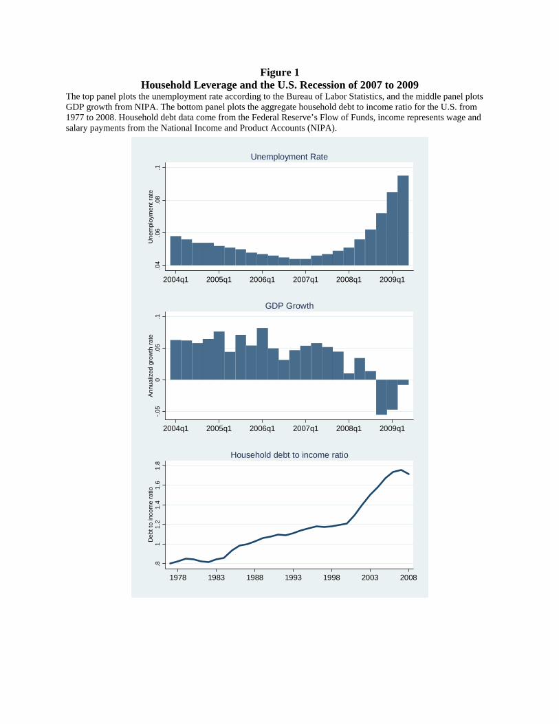
Figure 1 Household Leverage and the U.S. Recession of 2007 to 2009
The top panel plots the unemployment rate according to the Bureau of Labor Statistics, and the middle panel plots GDP growth from NIPA. The bottom panel plots the aggregate household debt to income ratio for the U.S. from 1977 to 2008. Household debt data come from the Federal Reserve’s Flow of Funds, income represents wage and salary payments from the National Income and Product Accounts (NIPA).
.04
.06
.08
.1U
nem
plo
yme
nt r
ate
2004q1 2005q1 2006q1 2007q1 2008q1 2009q1
Unemployment Rate-.
050
.05
.1A
nnua
lized
gro
wth
ra
te
2004q1 2005q1 2006q1 2007q1 2008q1 2009q1
GDP Growth
.81
1.2
1.4
1.6
1.8
De
bt t
o in
com
e r
atio
1978 1983 1988 1993 1998 2003 2008
Household debt to income ratio
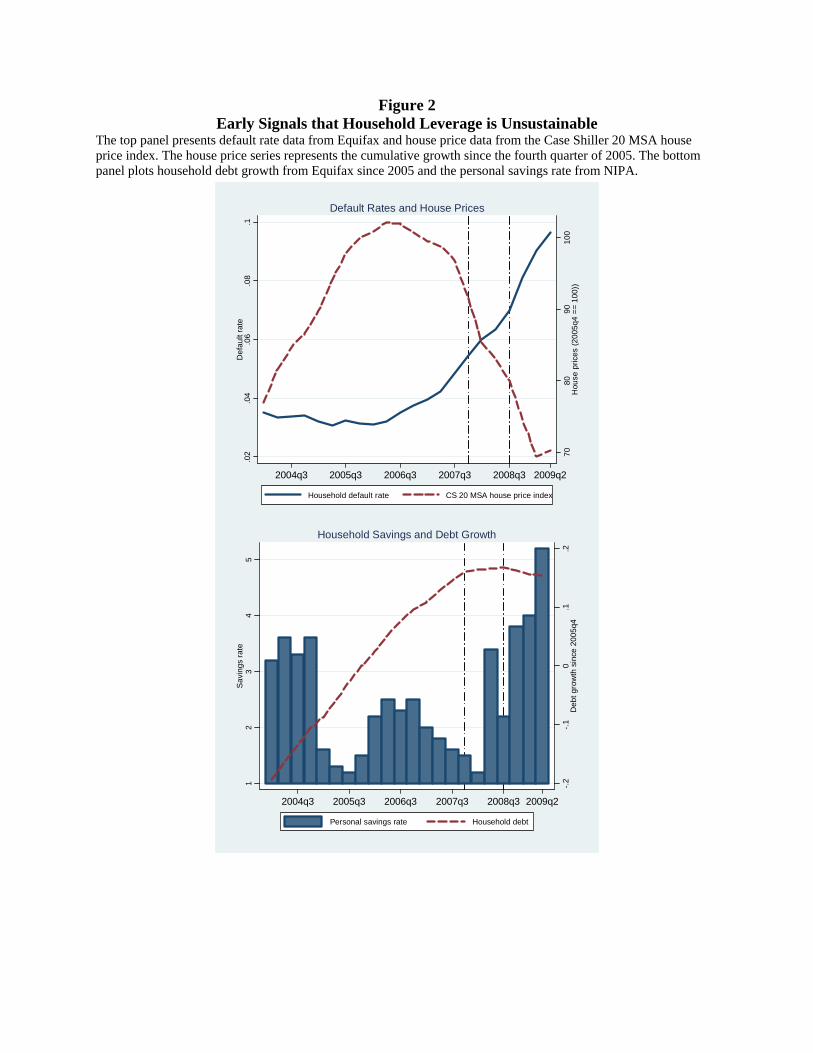
Figure 2 Early Signals that Household Leverage is Unsustainable
The top panel presents default rate data from Equifax and house price data from the Case Shiller 20 MSA house price index. The house price series represents the cumulative growth since the fourth quarter of 2005. The bottom panel plots household debt growth from Equifax since 2005 and the personal savings rate from NIPA.
70
80
90
10
0H
ou
se p
rice
s (2
00
5q
4 =
= 1
00
))
.02
.04
.06
.08
.1D
efa
ult
rate
2004q3 2005q3 2006q3 2007q3 2008q3 2009q2
Household default rate CS 20 MSA house price index
Default Rates and House Prices
-.2
-.1
0.1
.2D
eb
t g
row
th s
ince
20
05
q4
12
34
5S
avi
ng
s ra
te
2004q3 2005q3 2006q3 2007q3 2008q3 2009q2
Personal savings rate Household debt
Household Savings and Debt Growth
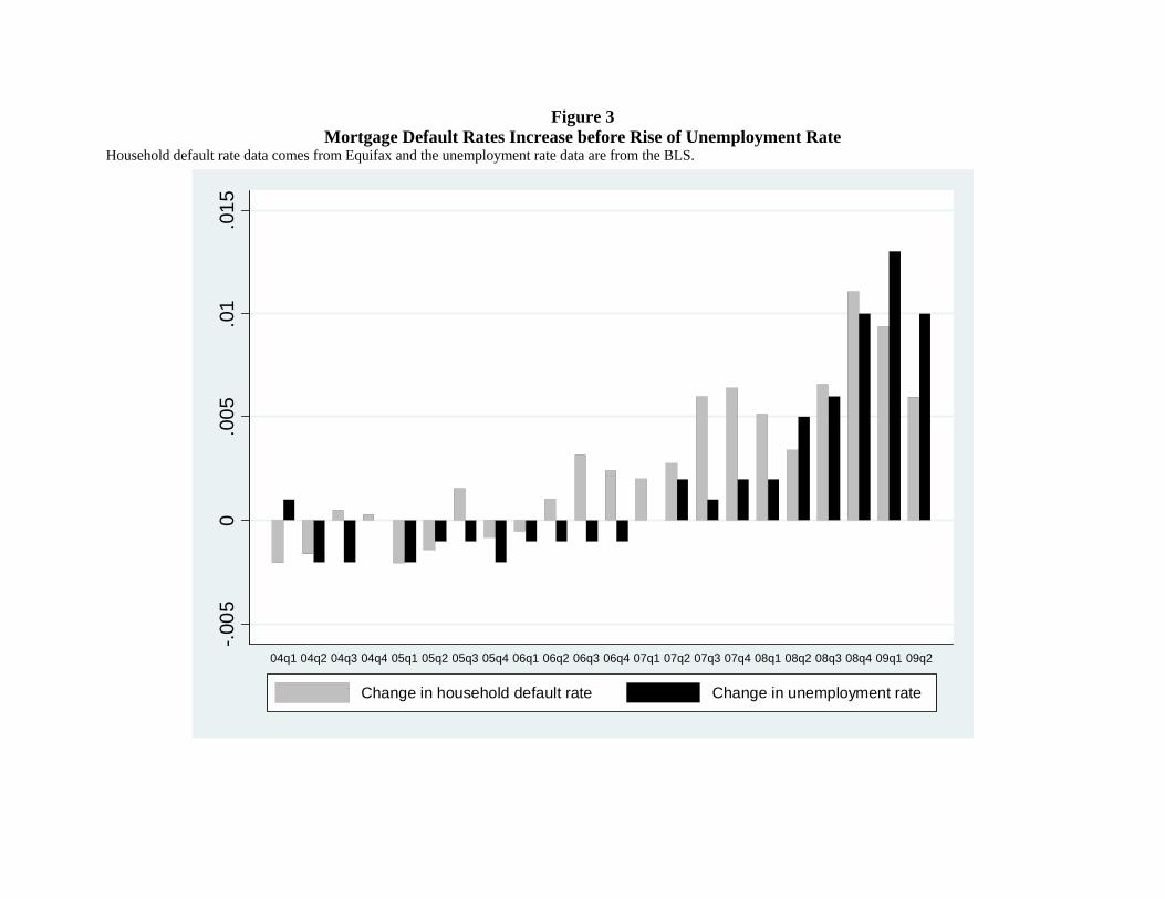
Figure 3 Mortgage Default Rates Increase before Rise of Unemployment Rate
Household default rate data comes from Equifax and the unemployment rate data are from the BLS.
-.00
50
.00
5.0
1.0
15
04q1 04q2 04q3 04q4 05q1 05q2 05q3 05q4 06q1 06q2 06q3 06q4 07q1 07q2 07q3 07q4 08q1 08q2 08q3 08q4 09q1 09q2
Change in household default rate Change in unemployment rate
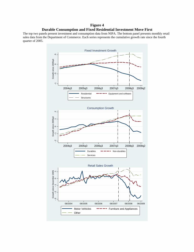
Figure 4 Durable Consumption and Fixed Residential Investment Move First
The top two panels present investment and consumption data from NIPA. The bottom panel presents monthly retail sales data from the Department of Commerce. Each series represents the cumulative growth rate since the fourth quarter of 2005.
-1-.
50
.5G
row
th s
ince
20
05q
4
2004q3 2005q3 2006q3 2007q3 2008q3 2009q2
Residential Equipment and software
Structures
Fixed Investment Growth
-.2
-.1
0.1
.2G
row
th s
ince
20
05
q4
2004q3 2005q3 2006q3 2007q3 2008q3 2009q2
Durables Non-durables
Services
Consumption Growth
-.3
-.2
-.1
0.1
Gro
wth
sin
ce D
ece
mb
er
20
05
08/2004 08/2005 08/2006 08/2007 08/2008 06/2009
Motor Vehicles Furniture and Appliances
Other
Retail Sales Growth
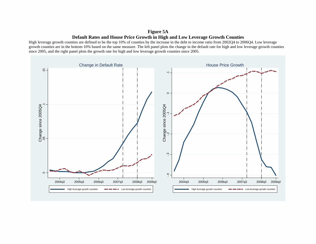
Figure 5A Default Rates and House Price Growth in High and Low Leverage Growth Counties
High leverage growth counties are defined to be the top 10% of counties by the increase in the debt to income ratio from 2002Q4 to 2006Q4. Low leverage growth counties are in the bottom 10% based on the same measure. The left panel plots the change in the default rate for high and low leverage growth counties since 2005, and the right panel plots the growth rate for high and low leverage growth counties since 2005.
0.0
5.1
.15
Cha
nge
sinc
e 20
05Q
4
2004q3 2005q3 2006q3 2007q3 2008q3 2009q2
High leverage growth counties Low leverage growth counties
Change in Default Rate
-.4
-.3
-.2
-.1
0.1
Cha
nge
sinc
e 20
05Q
4
2004q3 2005q3 2006q3 2007q3 2008q3 2009q2
High leverage growth counties Low leverage growth counties
House Price Growth
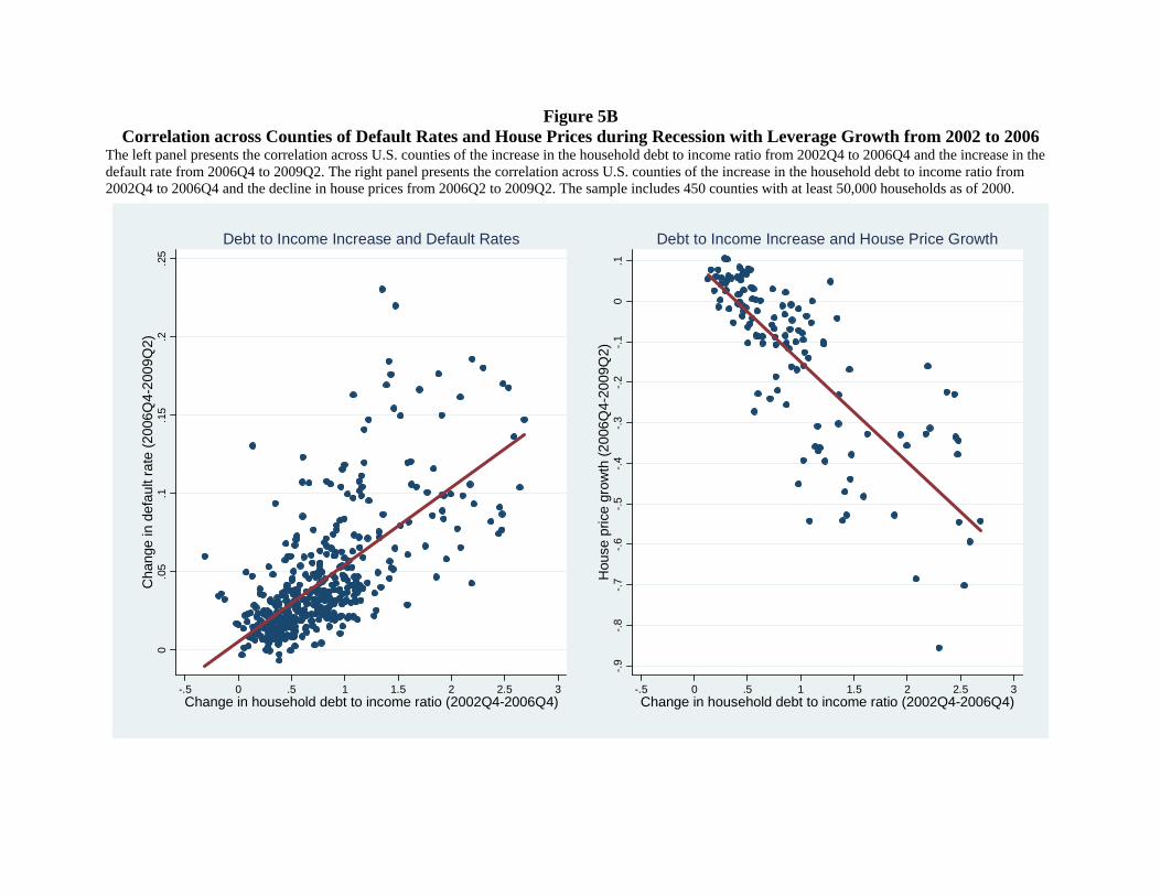
Figure 5B Correlation across Counties of Default Rates and House Prices during Recession with Leverage Growth from 2002 to 2006
The left panel presents the correlation across U.S. counties of the increase in the household debt to income ratio from 2002Q4 to 2006Q4 and the increase in the default rate from 2006Q4 to 2009Q2. The right panel presents the correlation across U.S. counties of the increase in the household debt to income ratio from 2002Q4 to 2006Q4 and the decline in house prices from 2006Q2 to 2009Q2. The sample includes 450 counties with at least 50,000 households as of 2000.
0.0
5.1
.15
.2.2
5C
hang
e in
def
ault
rate
(20
06Q
4-20
09Q
2)
-.5 0 .5 1 1.5 2 2.5 3Change in household debt to income ratio (2002Q4-2006Q4)
Debt to Income Increase and Default Rates
-.9
-.8
-.7
-.6
-.5
-.4
-.3
-.2
-.1
0.1
Hou
se p
rice
grow
th (
2006
Q4-
2009
Q2)
-.5 0 .5 1 1.5 2 2.5 3Change in household debt to income ratio (2002Q4-2006Q4)
Debt to Income Increase and House Price Growth
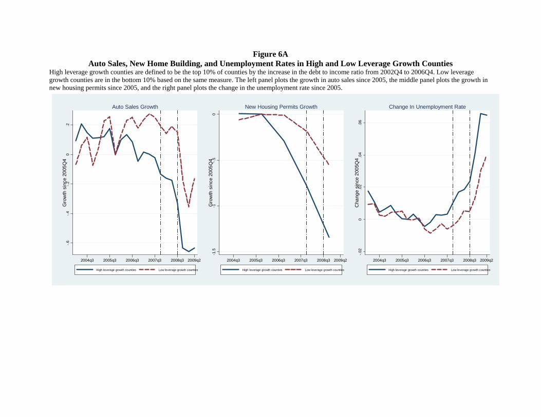
Figure 6A Auto Sales, New Home Building, and Unemployment Rates in High and Low Leverage Growth Counties
High leverage growth counties are defined to be the top 10% of counties by the increase in the debt to income ratio from 2002Q4 to 2006Q4. Low leverage growth counties are in the bottom 10% based on the same measure. The left panel plots the growth in auto sales since 2005, the middle panel plots the growth in new housing permits since 2005, and the right panel plots the change in the unemployment rate since 2005.
-.6
-.4
-.2
0.2
Gro
wth
sin
ce 2
005
Q4
2004q3 2005q3 2006q3 2007q3 2008q3 2009q2
High leverage growth counties Low leverage growth counties
Auto Sales Growth
-1.5
-1-.
50
Gro
wth
sin
ce 2
005
Q4
2004q3 2005q3 2006q3 2007q3 2008q3 2009q2
High leverage growth counties Low leverage growth counties
New Housing Permits Growth
-.02
0.0
2.0
4.0
6C
hang
e si
nce
200
5Q4
2004q3 2005q3 2006q3 2007q3 2008q3 2009q2
High leverage growth counties Low leverage growth counties
Change In Unemployment Rate
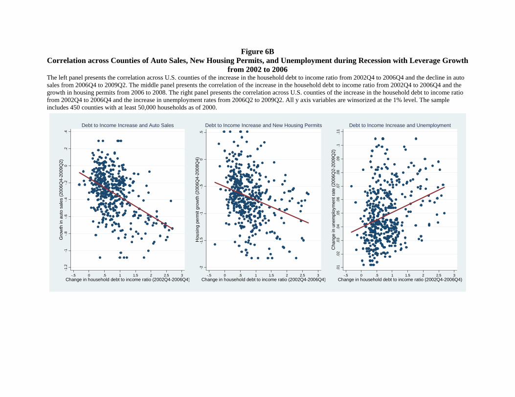
Figure 6B Correlation across Counties of Auto Sales, New Housing Permits, and Unemployment during Recession with Leverage Growth
from 2002 to 2006 The left panel presents the correlation across U.S. counties of the increase in the household debt to income ratio from 2002Q4 to 2006Q4 and the decline in auto sales from 2006Q4 to 2009Q2. The middle panel presents the correlation of the increase in the household debt to income ratio from 2002Q4 to 2006Q4 and the growth in housing permits from 2006 to 2008. The right panel presents the correlation across U.S. counties of the increase in the household debt to income ratio from 2002Q4 to 2006Q4 and the increase in unemployment rates from 2006Q2 to 2009Q2. All y axis variables are winsorized at the 1% level. The sample includes 450 counties with at least 50,000 households as of 2000.
-1.2
-1-.
8-.
6-.
4-.
20
.2.4
Gro
wth
in a
uto
sale
s (2
006
Q4-
2009
Q2)
-.5 0 .5 1 1.5 2 2.5 3Change in household debt to income ratio (2002Q4-2006Q4)
Debt to Income Increase and Auto Sales
-2-1
.5-1
-.5
0.5
Hou
sin
g pe
rmit
gro
wth
(2
006Q
4-2
008Q
4)
-.5 0 .5 1 1.5 2 2.5 3Change in household debt to income ratio (2002Q4-2006Q4)
Debt to Income Increase and New Housing Permits
.01
.02
.03
.04
.05
.06
.07
.08
.09
.1.1
1C
hang
e in
un
emp
loym
ent r
ate
(20
06Q
2-20
09Q
2)
-.5 0 .5 1 1.5 2 2.5 3Change in household debt to income ratio (2002Q4-2006Q4)
Debt to Income Increase and Unemployment
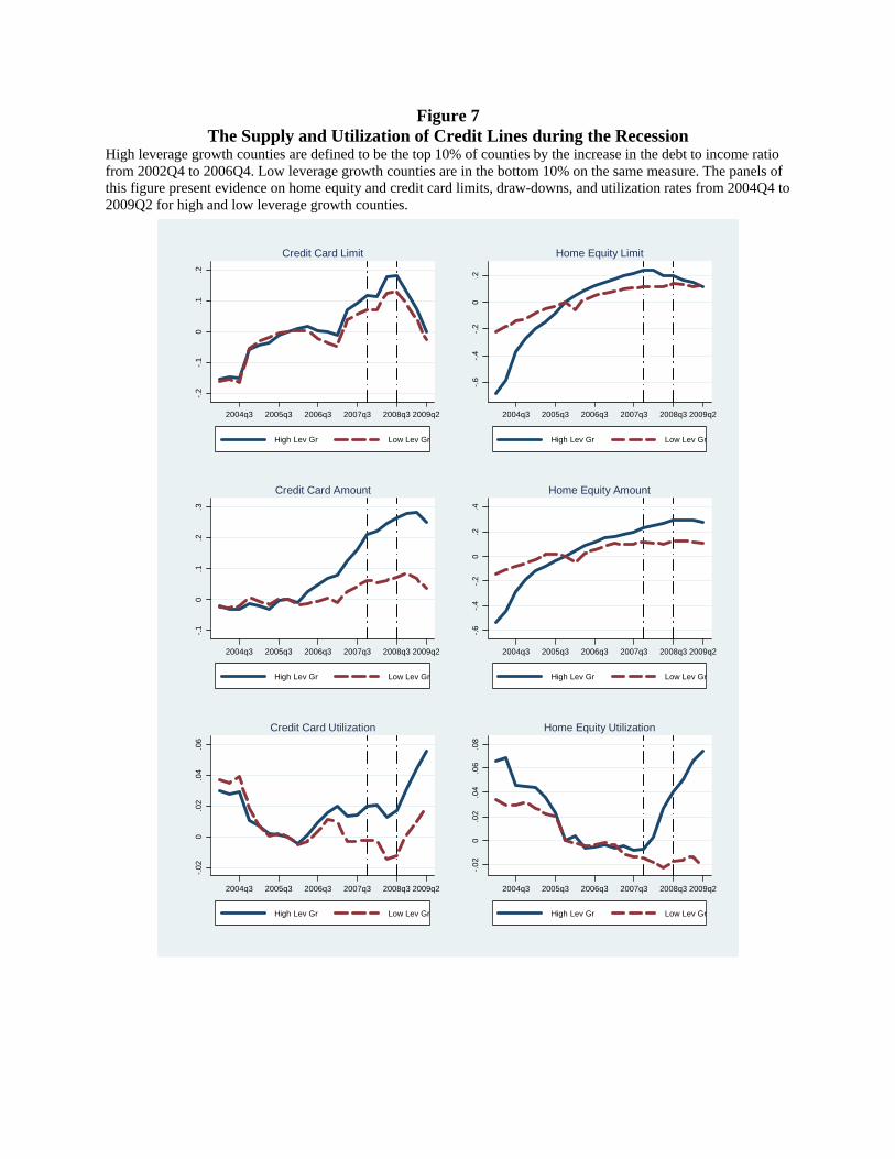
Figure 7 The Supply and Utilization of Credit Lines during the Recession
High leverage growth counties are defined to be the top 10% of counties by the increase in the debt to income ratio from 2002Q4 to 2006Q4. Low leverage growth counties are in the bottom 10% on the same measure. The panels of this figure present evidence on home equity and credit card limits, draw-downs, and utilization rates from 2004Q4 to 2009Q2 for high and low leverage growth counties.
-.2
-.1
0.1
.2
2004q3 2005q3 2006q3 2007q3 2008q3 2009q2
High Lev Gr Low Lev Gr
Credit Card Limit
-.6
-.4
-.2
0.2
2004q3 2005q3 2006q3 2007q3 2008q3 2009q2
High Lev Gr Low Lev Gr
Home Equity Limit
-.1
0.1
.2.3
2004q3 2005q3 2006q3 2007q3 2008q3 2009q2
High Lev Gr Low Lev Gr
Credit Card Amount
-.6
-.4
-.2
0.2
.4
2004q3 2005q3 2006q3 2007q3 2008q3 2009q2
High Lev Gr Low Lev Gr
Home Equity Amount
-.0
20
.02
.04
.06
2004q3 2005q3 2006q3 2007q3 2008q3 2009q2
High Lev Gr Low Lev Gr
Credit Card Utilization
-.0
20
.02
.04
.06
.08
2004q3 2005q3 2006q3 2007q3 2008q3 2009q2
High Lev Gr Low Lev Gr
Home Equity Utilization
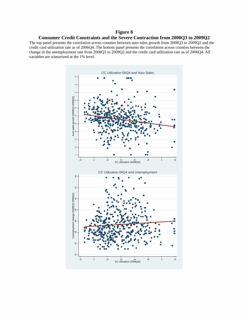
Figure 8 Consumer Credit Constraints and the Severe Contraction from 2008Q3 to 2009Q2
The top panel presents the correlation across counties between auto sales growth from 2008Q3 to 2009Q2 and the credit card utilization rate as of 2006Q4. The bottom panel presents the correlation across counties between the change in the unemployment rate from 2008Q3 to 2009Q2 and the credit card utilization rate as of 2006Q4. All variables are winsorized at the 1% level.
-.7
-.6
-.5
-.4
-.3
-.2
-.1
0.1
.2.3
Au
to s
ale
s g
row
th (
20
08
Q3
-20
09
Q2
)
.18 .2 .22 .24 .26 .28 .3 .32CC utilization (2006Q4)
CC Utilization 06Q4 and Auto Sales.0
1.0
2.0
3.0
4.0
5.0
6.0
7.0
8U
ne
mp
loym
en
t ch
an
ge
(2
00
8Q
3-2
00
9Q
2)
.18 .2 .22 .24 .26 .28 .3 .32CC utilization (2006Q4)
CC Utilization 06Q4 and Unemployment
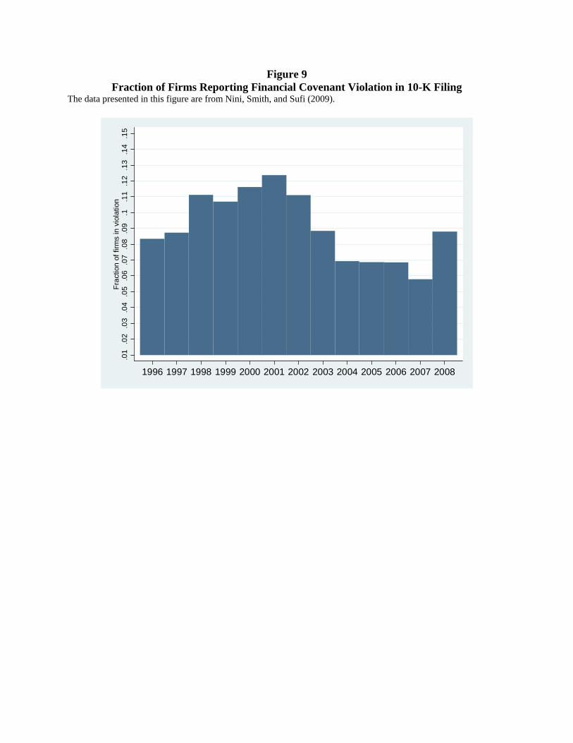
Figure 9 Fraction of Firms Reporting Financial Covenant Violation in 10-K Filing
The data presented in this figure are from Nini, Smith, and Sufi (2009).
.01
.02
.03
.04
.05
.06
.07
.08
.09
.1.1
1.1
2.1
3.1
4.1
5F
ract
ion
of f
irm
s in
vio
latio
n
1996 1997 1998 1999 2000 2001 2002 2003 2004 2005 2006 2007 2008
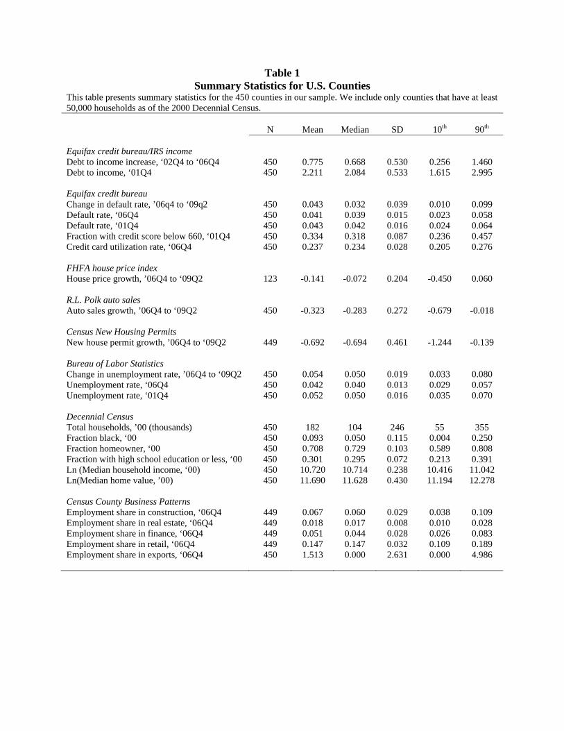
Table 1 Summary Statistics for U.S. Counties
This table presents summary statistics for the 450 counties in our sample. We include only counties that have at least 50,000 households as of the 2000 Decennial Census. N Mean Median SD 10th 90th Equifax credit bureau/IRS income Debt to income increase, ‘02Q4 to ‘06Q4 450 0.775 0.668 0.530 0.256 1.460 Debt to income, ‘01Q4 450 2.211 2.084 0.533 1.615 2.995 Equifax credit bureau Change in default rate, ’06q4 to ‘09q2 450 0.043 0.032 0.039 0.010 0.099 Default rate, ‘06Q4 450 0.041 0.039 0.015 0.023 0.058 Default rate, ‘01Q4 450 0.043 0.042 0.016 0.024 0.064 Fraction with credit score below 660, ‘01Q4 450 0.334 0.318 0.087 0.236 0.457 Credit card utilization rate, ‘06Q4 450 0.237 0.234 0.028 0.205 0.276 FHFA house price index House price growth, ’06Q4 to ‘09Q2 123 -0.141 -0.072 0.204 -0.450 0.060 R.L. Polk auto sales Auto sales growth, ’06Q4 to ‘09Q2 450 -0.323 -0.283 0.272 -0.679 -0.018 Census New Housing Permits New house permit growth, ’06Q4 to ‘09Q2 449 -0.692 -0.694 0.461 -1.244 -0.139 Bureau of Labor Statistics Change in unemployment rate, ’06Q4 to ‘09Q2 450 0.054 0.050 0.019 0.033 0.080 Unemployment rate, ‘06Q4 450 0.042 0.040 0.013 0.029 0.057 Unemployment rate, ‘01Q4 450 0.052 0.050 0.016 0.035 0.070 Decennial Census Total households, ’00 (thousands) 450 182 104 246 55 355 Fraction black, ‘00 450 0.093 0.050 0.115 0.004 0.250 Fraction homeowner, ‘00 450 0.708 0.729 0.103 0.589 0.808 Fraction with high school education or less, ‘00 450 0.301 0.295 0.072 0.213 0.391 Ln (Median household income, ‘00) 450 10.720 10.714 0.238 10.416 11.042 Ln(Median home value, ’00) 450 11.690 11.628 0.430 11.194 12.278 Census County Business Patterns Employment share in construction, ‘06Q4 449 0.067 0.060 0.029 0.038 0.109 Employment share in real estate, ‘06Q4 449 0.018 0.017 0.008 0.010 0.028 Employment share in finance, ‘06Q4 449 0.051 0.044 0.028 0.026 0.083 Employment share in retail, ‘06Q4 449 0.147 0.147 0.032 0.109 0.189 Employment share in exports, ‘06Q4 450 1.513 0.000 2.631 0.000 4.986

Table 2 The Effect of Household Leverage Increase from 2002Q4 to 2006Q4 on
Default Rates from 2006Q4 to 2009Q2 The regression in columns 2 through 5 are weighted by the number of households in the county as of 2000. Column 5 reports coefficients from the second stage of an IV specification where the change in the debt to income ratio from 2002 to 2006 is instrumented with housing supply inelasticity of the county as constructed by Saiz (2008). Standard errors are clustered by state. Dependent variable: Change in default rates, ‘06Q4 to ‘09Q2 (1) (2) (3) (4) (5) Unweighted Weighted Weighted Weighted Weighted
IV Change in debt to income, ‘02 to ‘06 0.049** 0.058** 0.056** 0.055** 0.093** (0.008) (0.009) (0.009) (0.009) (0.025) Debt to income, ‘01 0.020** 0.015* 0.010 (0.006) (0.006) (0.010) Unemployment rate, ‘06 -0.782 -0.520 -0.986* (0.474) (0.429) (0.429) Unemployment rate, ‘01 0.850** 0.767* 1.134** (0.313) (0.301) (0.349) Default rate, ‘06 -0.171 -0.228 -0.486 (0.246) (0.259) (0.323) Default rate, ‘01 1.280** 1.232** 1.642** (0.342) (0.360) (0.388) Fraction with credit score under 660, ‘01 0.245** 0.239** 0.093 (0.075) (0.082) (0.131) Credit card utilization rate, ‘06 -0.628** -0.610** -0.232 (0.130) (0.138) (0.325) Fraction black, ‘00 -0.066** -0.063* -0.049+ (0.025) (0.025) (0.027) Fraction homeowner, ‘00 -0.074* -0.049 -0.088 (0.031) (0.036) (0.054) Fraction with high school or less, ‘00 0.116* 0.131* 0.241** (0.053) (0.050) (0.065) Ln (Median household income, ‘00) 0.081** 0.072** 0.104** (0.022) (0.022) (0.033) Ln(Median home value, ’00) -0.021+ -0.018 -0.052* (0.012) (0.012) (0.021) Employment share in construction, ‘06 0.101 -0.059 (0.107) (0.114) Employment share in real estate, ‘06 0.770* 0.960* (0.382) (0.425) Employment share in finance, ‘06 0.066 0.066 (0.056) (0.096) Employment share in retail, ‘06 -0.048 -0.062 (0.062) (0.094) Employment share in exports, ‘06 -0.001 -0.000 (0.001) (0.001) Constant 0.005+ 0.005 -0.630** -0.595** -0.617* (0.003) (0.005) (0.153) (0.153) (0.238) Number of counties 450 450 450 449 218 R2 0.45 0.49 0.76 0.77 0.77 **,*,+ Coefficient estimate statistically distinct from 0 at the 1%, 5%, and 10% levels, respectively.

Table 3 The Effect of Household Leverage Increase from 2002Q4 to 2006Q4 on
House Price Growth from 2006Q4 to 2009Q2 The regression in columns 2 through 5 are weighted by the number of households in the county as of 2000. Column 5 reports coefficients from the second stage of an IV specification where the change in the debt to income ratio from 2002 to 2006 is instrumented with housing supply inelasticity of the county as constructed by Saiz (2008). Standard errors are clustered by state. Dependent variable: House price growth, ‘06Q4 to ‘09Q2 (1) (2) (3) (4) (5) Unweighted Weighted Weighted Weighted Weighted
IV Change in debt to income, ‘02 to ‘06 -0.247** -0.235** -0.221** -0.221** -0.553 (0.024) (0.032) (0.036) (0.035) (0.574) Debt to income, ‘01 -0.117* -0.079+ 0.076 (0.050) (0.044) (0.385) Unemployment rate, ‘06 -0.985 -0.760 -0.144 (1.798) (2.106) (2.938) Unemployment rate, ‘01 -1.523 -2.007 -4.407 (1.365) (1.359) (3.122) Default rate, ‘06 -2.661 -2.877 3.918 (2.061) (2.223) (14.229) Default rate, ‘01 -0.341 -0.809 -3.204 (1.891) (2.080) (6.192) Fraction with credit score under 660, ‘01 -1.523* -1.263* -0.384 (0.597) (0.593) (1.675) Credit card utilization rate, ‘06 4.261** 4.017** 0.602 (0.793) (0.762) (7.349) Fraction black, ‘00 0.262 0.220 0.303 (0.226) (0.220) (0.490) Fraction homeowner, ‘00 0.466+ 0.394 0.267 (0.230) (0.249) (0.816) Fraction with high school or less, ‘00 -0.417 -0.345 -0.939 (0.309) (0.291) (1.065) Ln (Median household income, ‘00) -0.575** -0.460** -0.929* (0.149) (0.141) (0.409) Ln(Median home value, ’00) 0.251** 0.199** 0.615 (0.062) (0.072) (0.468) Employment share in construction, ‘06 -1.132* 0.546 (0.456) (1.563) Employment share in real estate, ‘06 -0.790 -1.782 (1.449) (4.917) Employment share in finance, ‘06 -0.221 0.801 (0.279) (1.758) Employment share in retail, ‘06 0.797 4.587 (0.708) (5.352) Employment share in exports, ‘06 -0.004 0.012 (0.006) (0.028) Constant 0.097** 0.060 3.069* 2.395* 2.483 (0.023) (0.039) (1.206) (0.988) (3.873) Number of counties 123 123 123 123 56 R2 0.62 0.57 0.79 0.80 0.46 **,*,+ Coefficient estimate statistically distinct from 0 at the 1%, 5%, and 10% levels, respectively.
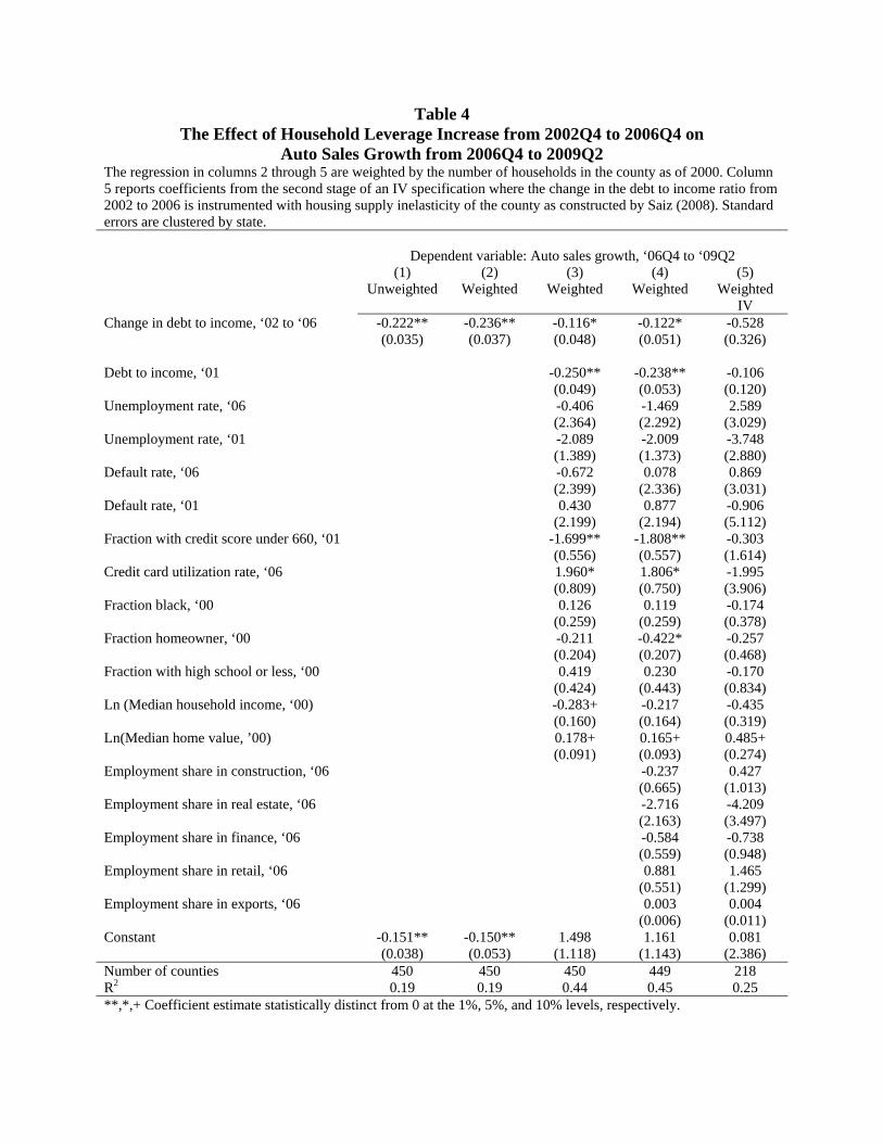
Table 4 The Effect of Household Leverage Increase from 2002Q4 to 2006Q4 on
Auto Sales Growth from 2006Q4 to 2009Q2 The regression in columns 2 through 5 are weighted by the number of households in the county as of 2000. Column 5 reports coefficients from the second stage of an IV specification where the change in the debt to income ratio from 2002 to 2006 is instrumented with housing supply inelasticity of the county as constructed by Saiz (2008). Standard errors are clustered by state. Dependent variable: Auto sales growth, ‘06Q4 to ‘09Q2 (1) (2) (3) (4) (5) Unweighted Weighted Weighted Weighted Weighted
IV Change in debt to income, ‘02 to ‘06 -0.222** -0.236** -0.116* -0.122* -0.528 (0.035) (0.037) (0.048) (0.051) (0.326) Debt to income, ‘01 -0.250** -0.238** -0.106 (0.049) (0.053) (0.120) Unemployment rate, ‘06 -0.406 -1.469 2.589 (2.364) (2.292) (3.029) Unemployment rate, ‘01 -2.089 -2.009 -3.748 (1.389) (1.373) (2.880) Default rate, ‘06 -0.672 0.078 0.869 (2.399) (2.336) (3.031) Default rate, ‘01 0.430 0.877 -0.906 (2.199) (2.194) (5.112) Fraction with credit score under 660, ‘01 -1.699** -1.808** -0.303 (0.556) (0.557) (1.614) Credit card utilization rate, ‘06 1.960* 1.806* -1.995 (0.809) (0.750) (3.906) Fraction black, ‘00 0.126 0.119 -0.174 (0.259) (0.259) (0.378) Fraction homeowner, ‘00 -0.211 -0.422* -0.257 (0.204) (0.207) (0.468) Fraction with high school or less, ‘00 0.419 0.230 -0.170 (0.424) (0.443) (0.834) Ln (Median household income, ‘00) -0.283+ -0.217 -0.435 (0.160) (0.164) (0.319) Ln(Median home value, ’00) 0.178+ 0.165+ 0.485+ (0.091) (0.093) (0.274) Employment share in construction, ‘06 -0.237 0.427 (0.665) (1.013) Employment share in real estate, ‘06 -2.716 -4.209 (2.163) (3.497) Employment share in finance, ‘06 -0.584 -0.738 (0.559) (0.948) Employment share in retail, ‘06 0.881 1.465 (0.551) (1.299) Employment share in exports, ‘06 0.003 0.004 (0.006) (0.011) Constant -0.151** -0.150** 1.498 1.161 0.081 (0.038) (0.053) (1.118) (1.143) (2.386) Number of counties 450 450 450 449 218 R2 0.19 0.19 0.44 0.45 0.25 **,*,+ Coefficient estimate statistically distinct from 0 at the 1%, 5%, and 10% levels, respectively.
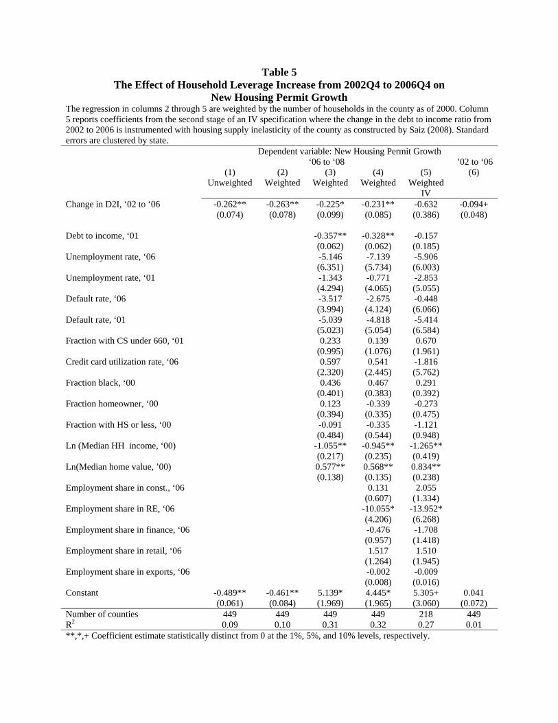
Table 5 The Effect of Household Leverage Increase from 2002Q4 to 2006Q4 on
New Housing Permit Growth The regression in columns 2 through 5 are weighted by the number of households in the county as of 2000. Column 5 reports coefficients from the second stage of an IV specification where the change in the debt to income ratio from 2002 to 2006 is instrumented with housing supply inelasticity of the county as constructed by Saiz (2008). Standard errors are clustered by state. Dependent variable: New Housing Permit Growth ‘06 to ‘08 ’02 to ‘06 (1) (2) (3) (4) (5) (6) Unweighted Weighted Weighted Weighted Weighted
IV
Change in D2I, ‘02 to ‘06 -0.262** -0.263** -0.225* -0.231** -0.632 -0.094+ (0.074) (0.078) (0.099) (0.085) (0.386) (0.048) Debt to income, ‘01 -0.357** -0.328** -0.157 (0.062) (0.062) (0.185) Unemployment rate, ‘06 -5.146 -7.139 -5.906 (6.351) (5.734) (6.003) Unemployment rate, ‘01 -1.343 -0.771 -2.853 (4.294) (4.065) (5.055) Default rate, ‘06 -3.517 -2.675 -0.448 (3.994) (4.124) (6.066) Default rate, ‘01 -5.039 -4.818 -5.414 (5.023) (5.054) (6.584) Fraction with CS under 660, ‘01 0.233 0.139 0.670 (0.995) (1.076) (1.961) Credit card utilization rate, ‘06 0.597 0.541 -1.816 (2.320) (2.445) (5.762) Fraction black, ‘00 0.436 0.467 0.291 (0.401) (0.383) (0.392) Fraction homeowner, ‘00 0.123 -0.339 -0.273 (0.394) (0.335) (0.475) Fraction with HS or less, ‘00 -0.091 -0.335 -1.121 (0.484) (0.544) (0.948) Ln (Median HH income, ‘00) -1.055** -0.945** -1.265** (0.217) (0.235) (0.419) Ln(Median home value, ’00) 0.577** 0.568** 0.834** (0.138) (0.135) (0.238) Employment share in const., ‘06 0.131 2.055 (0.607) (1.334) Employment share in RE, ‘06 -10.055* -13.952* (4.206) (6.268) Employment share in finance, ‘06 -0.476 -1.708 (0.957) (1.418) Employment share in retail, ‘06 1.517 1.510 (1.264) (1.945) Employment share in exports, ‘06 -0.002 -0.009 (0.008) (0.016) Constant -0.489** -0.461** 5.139* 4.445* 5.305+ 0.041 (0.061) (0.084) (1.969) (1.965) (3.060) (0.072) Number of counties 449 449 449 449 218 449 R2 0.09 0.10 0.31 0.32 0.27 0.01 **,*,+ Coefficient estimate statistically distinct from 0 at the 1%, 5%, and 10% levels, respectively.

Table 6 The Effect of Household Leverage Increase from 2002Q4 to 2006Q4 on
Change in Unemployment Rate from 2006Q4 to 2009Q2 The regression in columns 2 through 5 are weighted by the number of households in the county as of 2000. Column 5 reports coefficients from the second stage of an IV specification where the change in the debt to income ratio from 2002 to 2006 is instrumented with housing supply inelasticity of the county as constructed by Saiz (2008). Standard errors are clustered by state. Dependent variable: Change in unemployment rate, ‘06Q4 to ‘09Q2 (1) (2) (3) (4) (5) Unweighted Weighted Weighted Weighted Weighted
IV Change in debt to income, ‘02 to ‘06 0.007* 0.011** 0.008* 0.011** 0.018* (0.003) (0.003) (0.004) (0.003) (0.008) Debt to income, ‘01 0.012** 0.013** 0.005 (0.003) (0.003) (0.005) Unemployment rate, ‘06 0.205 0.157 -0.257 (0.386) (0.377) (0.164) Unemployment rate, ‘01 0.321 0.347+ 0.093 (0.220) (0.200) (0.090) Default rate, ‘06 0.205 0.178 0.214 (0.206) (0.218) (0.185) Default rate, ‘01 0.116 0.124 0.015 (0.179) (0.178) (0.194) Fraction with credit score under 660, ‘01 -0.000 0.018 0.035 (0.046) (0.042) (0.050) Credit card utilization rate, ‘06 -0.090 -0.102 -0.112 (0.106) (0.110) (0.123) Fraction black, ‘00 0.023 0.017 0.000 (0.018) (0.018) (0.014) Fraction homeowner, ‘00 -0.005 0.021 -0.007 (0.025) (0.026) (0.018) Fraction with high school or less, ‘00 0.064** 0.073** 0.028 (0.021) (0.021) (0.020) Ln (Median household income, ‘00) 0.020 0.014 0.004 (0.014) (0.013) (0.011) Ln(Median home value, ’00) -0.003 -0.003 -0.007 (0.011) (0.009) (0.008) Employment share in construction, ‘06 -0.065 -0.075 (0.044) (0.046) Employment share in real estate, ‘06 0.219 0.005 (0.208) (0.155) Employment share in finance, ‘06 0.014 0.056+ (0.046) (0.032) Employment share in retail, ‘06 -0.133* -0.032 (0.054) (0.037) Employment share in exports, ‘06 0.001** 0.000 (0.000) (0.000) Constant 0.048** 0.047** -0.188+ -0.131 0.039 (0.003) (0.004) (0.111) (0.104) (0.091) Number of counties 450 450 450 449 218 R2 0.04 0.10 0.30 0.34 0.44 **,*,+ Coefficient estimate statistically distinct from 0 at the 1%, 5%, and 10% levels, respectively.
Table 7 Consumer Credit Constraints and the Deepening of the Recession from 2008Q3 to 2009Q2
This table presents coefficient estimates of the effect of credit card utilization rates on auto sales and unemployment. Column 3 (4) restricts the sample to firms in the bottom (top) decile counties of the change in debt to income from 2002 to 2006 distribution. The specification reported in column 3 includes the following control variables: the unemployment rate as of 2001Q4 and 2006Q4, the fraction of population that is black, the fraction of homeowners, the fraction with a high school education or less, and the fraction of employment in construction, real estate, finance, retail and export industries. All regressions are weighted by the number of households and standard errors are clustered by state.
Dependent variable Auto sales growth,
‘06Q4 to ‘08Q3
Auto sales growth, ‘06Q4 to ‘09Q2
Housing permit growth,
’06 to ‘08
Unemployment rate change,
‘06Q4 to ‘08Q3
Unemployment rate change,
‘06Q4 to ‘09Q2 (1) (2) (3) (4) (5) (6) Change in debt to income, ‘02 to ‘06 -0.194** -0.281** -0.264** -0.287** 0.010** 0.012** (0.023) (0.030) (0.056) (0.080) (0.001) (0.002) CC utilization rate, ‘06Q4 -1.066 -3.051** -1.664+ -1.580 0.034 0.085 (0.712) (0.688) (0.866) (1.158) (0.042) (0.083) Constant 0.309+ 0.616** -2.282+ -0.065 0.002 0.025 (0.181) (0.180) (1.280) (0.313) (0.010) (0.018) Control variables? N N Y N N N Number of counties 450 450 449 449 450 450 R2 0.30 0.26 0.37 0.11 0.20 0.11 **,*,+ Coefficient estimate statistically distinct from 0 at the 1%, 5%, and 10% levels, respectively.
Table 8 Can the Effect of Household Leverage on Recession Severity be Due to Local Banking Effects?
The coefficient estimates reported in columns 1 through 3 are from specifications that isolate the sample to counties where the banks have less than 10% of their deposits within the same county. Columns 4 through 6 report coefficient estimates from specifications that include measures of bank performance within the county. All specifications are weighted by the number of households in the county as of 2000. Standard errors are clustered by state. Only counties where banks have <10% local
deposits Include controls for performance of banks in
county (1) (2) (3) (4) (5) (6)
Dependent variable: Auto sales growth,
‘06q4 to ‘09q2
New Housing Permit Growth,
‘06 to ‘08
Increase in unemployment
rate, ‘06q4 to ‘09q2
Auto sales growth,
‘06q4 to ‘09q2
New Housing Permit Growth,
‘06 to ‘08
Increase in unemployment
rate, ‘06q4 to ‘09q2
Change in debt to income, ‘02 to ‘06 -0.219** -0.170** 0.007* -0.236** -0.255** 0.010** (0.035) (0.039) (0.003) (0.036) (0.064) (0.002) Change in charge-offs for banks in county, ’05 to ‘08 -2.334 2.255 -0.061 (2.464) (3.998) (0.132) Change in net income for banks in county, ’05 to ‘08 14.537* 25.300** -1.133** (5.609) (8.999) (0.343) Constant -0.172* -0.558** 0.053** -0.014 -0.307** 0.039** (0.066) (0.073) (0.005) (0.062) (0.089) (0.004) Number of counties 52 51 52 450 449 450 R2 0.30 0.08 0.10 0.25 0.16 0.18 **,*,+ Coefficient estimate statistically distinct from 0 at the 1%, 5%, and 10% levels, respectively.

Appendix Table 20% of Counties in Sample, Ordered by Change in Debt to Income from 2002 to 2006
(Largest Increase First) This table lists every 5th county in our sample, ordered by the largest increase in the household debt to income ratio from 2002 to 2006. There are a total of 450 counties in our sample, and 90 counties in this list.
1 CALIFORNIA,MONTEREY 46 FLORIDA,PASCO 2 CALIFORNIA,SANTABARBARA 47 KENTUCKY,KENTON 3 CALIFORNIA,MERCED 48 CONNECTICUT,TOLLAND 4 HAWAII,HAWAII 49 NEW MEXICO,BERNALILLO 5 VIRGINIA,LOUDOUN 50 GEORGIA,MUSCOGEE 6 FLORIDA,SARASOTA 51 INDIANA,LAKE 7 OREGON,DESCHUTES 52 WISCONSIN,MILWAUKEE 8 FLORIDA,MANATEE 53 WASHINGTON,SPOKANE 9 FLORIDA,CHARLOTTE 54 NORTH CAROLINA,DURHAM
10 MARYLAND,MONTGOMERY 55 MISSOURI,JACKSON 11 FLORIDA,BROWARD 56 MICHIGAN,KALAMAZOO 12 NEW JERSEY,OCEAN 57 WISCONSIN,OUTAGAMIE 13 COLORADO,BOULDER 58 FLORIDA,ALACHUA 14 MARYLAND,PRINCEGEORGES 59 TEXAS,FORTBEND 15 FLORIDA,OKALOOSA 60 OHIO,STARK 16 FLORIDA,CITRUS 61 WISCONSIN,ROCK 17 NEW JERSEY,MONMOUTH 62 TEXAS,SMITH 18 NEW YORK,ROCKLAND 63 INDIANA,ELKHART 19 MASSACHUSETTS,HAMPSHIRE 64 KANSAS,WYANDOTTE 20 COLORADO,ARAPAHOE 65 SOUTH CAROLINA,YORK 21 NEW YORK,RICHMOND 66 SOUTH CAROLINA,RICHLAND 22 COLORADO,JEFFERSON 67 NEW YORK,ALBANY 23 ILLINOIS,LAKE 68 PENNSYLVANIA,BERKS 24 FLORIDA,BAY 69 ARKANSAS,PULASKI 25 NEW JERSEY,SUSSEX 70 INDIANA,PORTER 26 MARYLAND,WASHINGTON 71 NORTH CAROLINA,MECKLENBURG 27 NEW JERSEY,UNION 72 KANSAS,SHAWNEE 28 ALASKA,ANCHORAGE 73 NEW YORK,RENSSELAER 29 ILLINOIS,COOK 74 NEW YORK,BRONX 30 WASHINGTON,SNOHOMISH 75 ILLINOIS,WINNEBAGO 31 MAINE,KENNEBEC 76 OREGON,MARION 32 FLORIDA,MARION 77 TENNESSEE,RUTHERFORD 33 NORTH CAROLINA,CABARRUS 78 TENNESSEE,SULLIVAN 34 INDIANA,MONROE 79 LOUISIANA,EASTBATONROUGE 35 NEW YORK,QUEENS 80 PENNSYLVANIA,LEBANON 36 COLORADO,WELD 81 TEXAS,MCLENNAN 37 GEORGIA,DEKALB 82 TEXAS,NUECES 38 MICHIGAN,GENESEE 83 TEXAS,BRAZORIA 39 NEW JERSEY,MIDDLESEX 84 TEXAS,TARRANT 40 MISSOURI,CLAY 85 PENNSYLVANIA,WESTMORELAND 41 MICHIGAN,OTTAWA 86 ILLINOIS,MACON 42 ARKANSAS,BENTON 87 ARIZONA,PINAL 43 UTAH,DAVIS 88 LOUISIANA,RAPIDES 44 MICHIGAN,MONROE 89 OHIO,RICHLAND 45 SOUTH CAROLINA,LEXINGTON 90 TEXAS,ECTOR


![PRESENTATION (ATIF,BILAL)[1].ppt](https://img.pdfslide.us/doc/110x75/553fc3f1550346e26f8b4909/presentation-atifbilal1ppt.jpg)