Embed Size (px)
Citation preview
House Prices and New Firm Capital Structure ∗
Kristoph Kleiner†
Indiana University, Kelley School of Business
Abstract
We examine how real estate prices impact new �rm capital structure. Relying a new micro-level
dataset, we �nd that during the housing boom one-quarter of large US entrepreneurs depended
on home equity as a source of initial capital. In response to an exogenous shock to real estate
price growth, start-ups increase reliance on home equity �nancing relative to �rms with minimal
�nancing needs. The results are greatest for �rms that receive between $50,000, and $1 million
in funding. In contrast, we see entrepreneurs shift �nancing away from formal business loans, yet
�nd minimal e�ects on informal debt markets (such as family and friends) or household credit
cards. Our results suggest that while home equity is a signi�cant source of �nancing, collateral
values have only a limited impact on capital structure outside of bank debt.
∗I thank my advisor Pat Bayer, and committee members Manuel Adelino, David Robinson, and Daniel Xu as thispaper is based on the third chapter of my PhD Dissertation. I thank seminar participants at Duke University and theFuqua School of Business. All remaining errors are my own.†Department of Finance, Indiana University, 1309 East 10th Street, Bloomington, IN 47405. Email: Klein-
1
1 Introduction
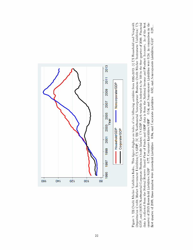
Between 1997 and 2009 the Debt-to-GDP ratio of US noncorporate �rms (sole proprietorships and
limited partnerships) grew faster than both household debt and corporate debt before subsequently
declining by 14% during the Financial Crisis as shown in Figure 1. Research has highlighted the
possibility that the rise and fall of small �rm debt is linked to the housing market as evidence �nds
that an increase in real estate prices leads to a higher likelihood of entrepreneurship [Hurst and Lusardi,
2004, Adelino et al., 2013, Schmalz et al., 2013, Corradin and Popov, 2015]. These papers rest on the
theory that collateral pledging alleviates �nancial frictions when contracts are incomplete Hart and
Moore [1995], and empirical evidence that �rms with high default risk are required to secure loans
through collateral Berger and Udell [1990].
To date, direct evidence of real estate prices on the capital structure of new �rms is still quite
limited. This is a noticeable gap given the literature on consumer borrowing has separately identi�ed
house price a�ects on both secondary mortgages [Mian and Su�, 2011] and consumption [Mian et al.,
2013]. Similarly, an alternate research agenda documents real estate price a�ects on both corporate
investment/employment [Chaney et al., 2012, Kleiner, 2014] and capital structure [Cvijanovic, 2014].
Using a new �rm-level dataset on US small �rm �nancing, we quantify the impact of house prices on
new �rm capital structure. We �rst o�er clear evidence that home equity is an economically signi�cant
source of �nancing. We �nd that in 2006 eleven percent of all start-ups relied on home equity to initially
fund the �rm. This number increases up to 29% of �rms with �nancing needs between $100,000 and
$249,999.
We next highlight the role of house price shocks in new �rm �nancing. To isolate this e�ect we
distinguish between �rms that take under $5,000 in initial �nancing and �rms over $5,000. This allows
us to separate local demand shocks-which a�ect all �rms- from collateral shocks that a�ect only �rms
with high �nancing needs.
There are two sources of endogeneity in our analysis. First, �rms with large �nancing needs may be
uniquely a�ected by local demand shocks. Secondly, initial �nancing needs are an endogenous choice.
To overcome the �rst concern we follow the literature and instrument for exogenous house price growth
2
from the housing supply elasticity measure �rst developed by Saiz [2010]. As discussed in Cvijanovic
[2014] the intuition for this approach is that local areas with little undeveloped land experience large
real estate price appreciation in response to an increase in the aggregate real estate demand. Areas
with available undeveloped land will experience more minor price growth since the demand can be
easily supplied.
We attempt to alleviate the second concern- �nancing needs are endogenous- in two ways. First, we
allow for both �rm and owner characteristics in the empirical speci�cation. Secondly, we extend our
analysis by developing a simple pseudo-panel. With panel data we are able control for unobservable
di�erences across �rms.
We estimate that a 10% real estate price growth increases home equity �nancing by 1.1% for the
mean �rm. We also calculate the probability a �rm �nances exclusively through this channel increases
by 0.4%. The results hold in the pseudo-panel estimation. The e�ects of real estate shocks are strongest
for large start-ups. Real estate price growth of 10% increases home equity �nancing by 2.1% for �rms
with been $250,000 and $1 million in initial �nancing.
Our collateral shock a�ects the capital structure of the �rm. In response to an exogenous shock
to real estate price growth, start-ups increase reliance on home equity �nancing, causing a decline in
�nancing through formal bank loans. Speci�cally, a 10% increase in real estate prices causes a 1.7%
decrease in the probability of bank lending. The results hold regardless of �rm �nancing needs and
industry. In comparison, house prices have no a�ect on costly consumer debt (such as credit cards) or
informal lending (such as family loans).
To highlight the policy implications of our results we focus on the e�ect of house prices on govern-
ment loan guaranteed programs. The rational for this type of intervention is that a lack of collateral is
a primary impediment for access to �nancing. This argument appears to hold as a ten percent increase
in real estate decreases government guaranteed loans by 0.12% and up to 0.3% for �rms with �nancing
between $25,000-$250,000. We conclude with a discussion and applicability of our results following the
2008 Financial Crisis.
A number of papers have theoretically documented the role of credit constraints in the entrepreneur-
3
ship decision, including Evans and Jovanovic [1989] and Cagetti and De Nardi [2006]. This theory
appears to hold up empirically: one line of the literature has focused on using house price growth as
a credit shock on small business. For instance Hurst and Lusardi [2004] document that prices impact
the decision to start a business, but only at the top of the wealth distribution. Recent evidence from
Adelino et al. [2013], Schmalz et al. [2013], Corradin and Popov [2015] instead highlights a strong
correlation between house price growth and new business starts. Missing from this analysis is an
understanding of the underlying capital structure.
Closest to our work, Robb and Robinson [2012] �nds that a positive real estate shock increases bank
loan �nancing. We extend this analysis in a number of ways. First, we develop a new identi�cation
strategy to distinguish demand e�ects from collateral e�ects. Secondly, we include direct information
on home equity �nancing, and so can distinguish secured vs. unsecured debt. Third, we characterize
the impact of real estate shocks to the full capital structure, as opposed to just bank debt. Fourth, we
include a much larger sample size, allowing for a number of robustness checks.
The outline for this paper is as follows. Section 2 introduces our empirical methodology and
summarizes the data. Section 3 discusses the results and Section 4 concludes.
2 Empirical Methodology and Data
The purpose of our paper is to �rst determine the role of home equity in small �rm �nancing, and
secondly, to evaluate the e�ect of house price shocks on capital structure. In this section, we determine
the empirical speci�cation necessary to achieve the latter goal, and then summarize the data to ful�ll
the former.
4
2.1 Empirical Methodology
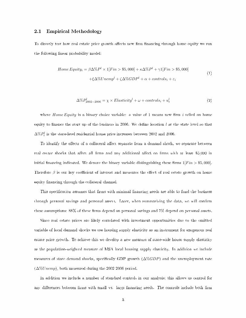
To directly test how real estate price growth a�ects new �rm �nancing through home equity we run
the following linear probability model:
HomeEquityi = β∆%P l × 1[Fin > $5, 000] + κ∆%P l + γ1[Fin > $5, 000]
+ξ∆%Unempl + ζ∆%GDP l + α+ controlsi + εi
(1)
∆%P l2002−2006 = χ× Elasticityl + ω + controlsi + ult (2)
where HomeEquity is a binary choice variable: a value of 1 means new �rm i relied on home
equity to �nance the start-up of the business in 2006. We de�ne location l at the state level so that
∆%P lt is the state-level residential house price increases between 2002 and 2006.
To identify the e�ects of a collateral a�ect separate from a demand shock, we separate between
real estate shocks that a�ect all �rms and any additional a�ect on �rms with at least $5,000 in
initial �nancing indicated. We denote the binary variable distinguishing these �rms 1[Fin > $5, 000].
Therefore β is our key coe�cient of interest and measures the e�ect of real estate growth on home
equity �nancing through the collateral channel.
This speci�cation assumes that �rms with minimal �nancing needs are able to fund the business
through personal savings and personal assets. Later, when summarizing the data, we will con�rm
these assumptions: 88% of these �rms depend on personal savings and 7% depend on personal assets.
Since real estate prices are likely correlated with investment opportunities due to the omitted
variable of local demand shocks we use housing supply elasticity as an instrument for exogenous real
estate price growth. To achieve this we develop a new measure of state-wide house supply elasticity
as the population-weighted measure of MSA local housing supply elasticity. In addition we include
measures of state demand shocks, speci�cally GDP growth (∆%GDP ) and the unemployment rate
(∆%Unemp), both measured during the 2002-2006 period.
In addition we include a number of standard controls in our analysis; this allows us control for
any di�erences between �rms with small vs. large �nancing needs. The controls include both �rm
5
characteristics (such as NAICS sector �xed e�ects and �rm size �xed e�ects) and owner characteristics
(such as number of owner, and educational background). Finally all results are clustered at the state
level.
In our �rst stage results we �nd that our state-level measure of housing supply elasticity is highly
correlated with real estate values between 2002 and 2006. A coe�cient of -0.25 implies that a one
standard deviation increase in elasticity decreases real estate price growth by 8 percentage points.
This re�ects that even at the state-level housing supply elasticity was a strong predictor of the run-up
of housing price growth documented between 2002 and 2006.
One concern with this analysis is that we are not able to control for unobservable �rm character-
istics as we only have cross-sectional data. This is a particular concern since �nancing needs is an
endogenous choice, yet we take the variable as exogenous in our methodology once controlling for all
other observable characteristics.
To alleviate this concern we rely on our large sample to also develop a pseudo-panel of our data by
characterizing a pseudo-�rm for each speci�c state and �nancing level pair. First introduced by Deaton
[1985], a pseudo-panel is an econometric technique to track cohorts through a series of independent
cross-sections, creating a new dataset of panel data.
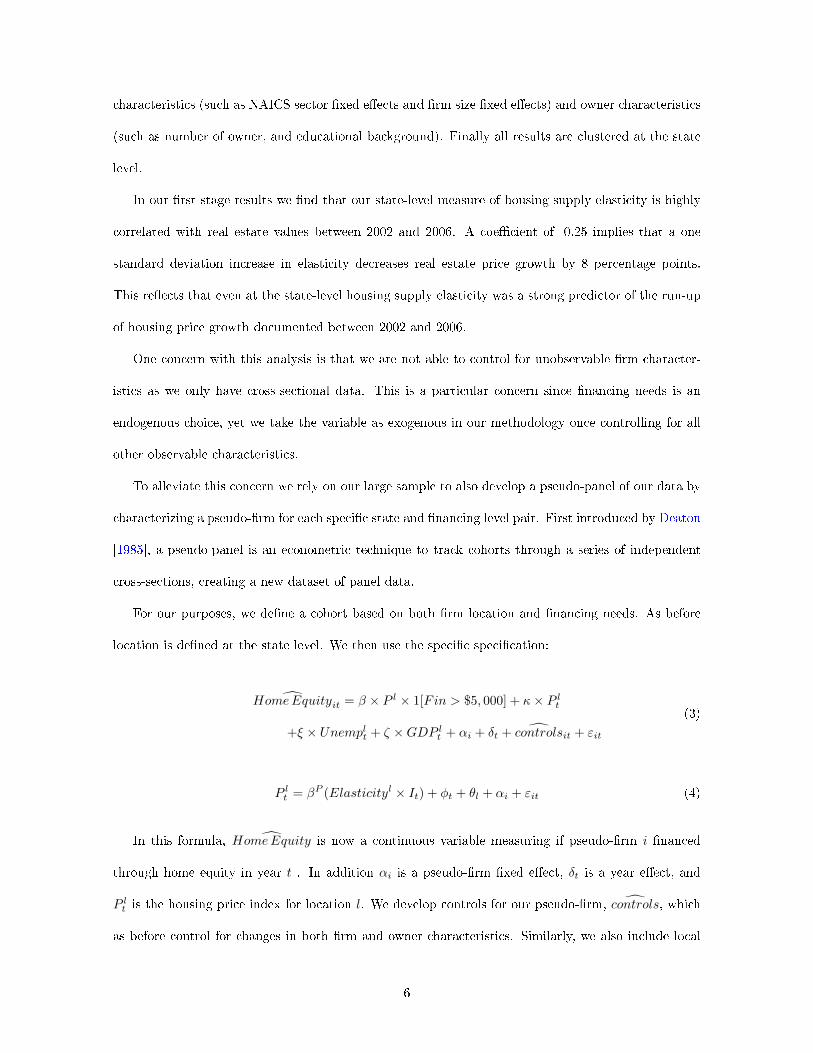
For our purposes, we de�ne a cohort based on both �rm location and �nancing needs. As before
location is de�ned at the state level. We then use the speci�c speci�cation:
HomeEquityit = β × P l × 1[Fin > $5, 000] + κ× P lt
+ξ × Unemplt + ζ ×GDP lt + αi + δt + controlsit + εit
(3)
P lt = βP (Elasticityl × It) + φt + θl + αi + εit (4)
In this formula, HomeEquity is now a continuous variable measuring if pseudo-�rm i �nanced
through home equity in year t . In addition αi is a pseudo-�rm �xed e�ect, δt is a year e�ect, and
P lt is the housing price index for location l. We develop controls for our pseudo-�rm, controls, which
as before control for changes in both �rm and owner characteristics. Similarly, we also include local
6
unemployment and GDP measures. An indicator for �nancing needs is now absorbed by the pseudo-
�rm �xed e�ect. The advantage to the speci�cation is that we are able to control for static unobservable
di�erences across �nancing need cohorts.
As before, our analysis relies on an exogenous source of real estate price growth; therefore we
also derive a time-varying instrument by interacting the conventional mortgage rate with the state-
level housing supply elasticity. The intuition in this speci�cation is that the national mortgage rate
is a measure of national house demand. Local demand shocks will most impact house price growth
in inelastic regions during periods of high national demand- and therefore low mortgage rates. The
speci�cation is similar to Chaney et al. [2012].
2.2 Data Summary
O�ce of Federal Housing Enterprise Oversight House Price Index
The OFHEO House Price Index is available at the state level starting in 1975 and for the majority
of Metropolitan Statistical Areas starting in 1987. For our purposes we focus on the state level data
between 2002 and 2006. During this time period we �nd signi�cant cross-sectional heterogeneity in
real estate price growth. Speci�cally, Michigan saw 10% and Indiana and Ohio saw an 11% increase
in house price between 2002 and 2006. In comparison Hawaii, Florida, Nevada, and California saw a
combined growth rate of 93%, 88%, 87%, and 86%, respectively.
Local Housing Supply Elasticity
The local housing supply elasticity measure comes from Saiz [2010] and is available for 95 MSAs.
It is estimated using processing satellite-generated data on elevation and presence of bodies of water.
Given our focus on state-level data, we develop a new measure of state housing supply elasticity:
speci�cally, we weight each MSA as a fraction of the population of the state. From our state-level
estimates we �nd a large range from an elasticity from 0.65 for New Hampshire, 0.69 for New Jersey
and New York to 2.83 for Nebraska and Iowa and 3.36 for Kansas.
7
Bureau of Economic Analysis State GDP
Due control for time-varying changes within a state, we also include data on both GDP and
unemployment. Our GDP data comes from the Bureau of Economic Analysis. We �nd that between
2002 and 2006 the median state saw an 11% increase in real GDP with the 10th and 90th percentiles
at 5% and 21%.
Bureau of Labor Statistics Unemployment Rate
The state-level unemployment rate is the Bureau of Labor statistics. The unemployment rate fell
about 1% in the average state with no change at the 90th percentile.
Survey of Small Business Owners
Our empirical analysis depends on a new �rm-level dataset from the Survey of Business Owners
(SBO) Public Use Microdata Sample (PUMS). The SBO PUMS is a cross-sectional dataset on en-
trepreneurs and surveys a random sample of business from a complete list of all �rms operating during
2007 with receipts of at least $1,000. The data include categorical variables documenting both the
�nancial needs of each �rm, and variables that denote the source of all initial funding and all later
funding.
The list of all forms is compiled from business tax returns, speci�cally: Form 1040 Schedule C
(Pro�t or Loss from Business), Form 1065 (US Return of Partnership Income), 1120 Corporation
Tax Forms, Form 941 �Employer's Quarterly Federal Tax Return�, and Form 944 �Employer's Annual
Federal Tax Return.
For �rms with paid employees, the Census Bureau also collected employment, payroll, receipts, and
kind of business for each plant, store, of location during the 2007 Economic Census. To control for
response bias, three report forms are re-mailed to employer �rms and two report forms are re-mailed
to nonemployer �rms at one month intervals to all delinquent respondents. We use the data between
2002 and 2007 for our results.
Publicly-held �rms are not excluded in initial data. Records for states with under 100,000 weighted
8
businesses are combined with records of similar states: Alaska and Wyoming are combined together,
as are Delaware and District of Columbia, North and South Dakota, and Rhode Island and Vermont.
For our purposes, we exclude all combined states. Finally, the survey data includes weights which are
used in our regression analysis.
We �rst note the magnitude of our sample at 949,169 �rms according to Table 1. Employment is
the mean number of employees per �rm, while all remaining variables are the percentage of �rms that
rely on the speci�ed external �nancing option.
In our summary statistics we distinguish cohorts by the level of initial received �nancing: (i)
less than $5,000, (ii) $5,000-9,999, (iii) $10,000-24,999, (iv) $25,000-49,999, (v) $50,000-99,999, (vi)
$100,000-249,999, (vii) $250,000-999,999, and (viii) greater than $1 million. In addition note that we
have nearly 40,000 �rms with �nancing needs of at least one million dollars on creation. Therefore our
sample covers a wide range of start-ups during the 2002-2007 period.
To give some indication we use survey weights to determine the actual proportion in the economy:
(i) less than $5,000 make up 51% of �rms (ii) $5,000-9,999 compose 12%, (iii) $10,000-24,999 represent
12%, (iv) $25,000-49,999 are 8% of the economy, (v) $50,000-99,999 are 7%, (vi) $100,000-249,999 are
6%, (vii) $250,000-999,999 compose 4% of all �rms, and (viii) greater than $1 million represent 1% of
initial businesses. Therefore, the larger �rms are actually overrepresented in our survey compared to
the true population.
New Firm Financing
From 1 we �nd that the mean �rm has 5.1 employees and over half of the �rms in our sample are
nonemployer �rms. Employment in the �rst cohort (�nancing under $5,000) is only 0.9 and increases
monotonically to 34.5 employees in the largest cohort (�nancing at least $1 million).
We consider a range of �nancial sources: owner equity (denoted here as savings and assets), house-
hold credit cards, formal business loans, home equity loans, informal debt (denoted here as family
loans), government-assisted debt (both government loans and government guaranteed loans), venture
capital, and grants.
We �nd strong evidence that larger �rms are more likely to rely on formal business loans. For
9
instance 81 percent of all �rms in the sample rely on some sort of savings and this value is largest for
the smallest cohort (88%) and declines with �rm �nancing needs to 57%. In comparison, 12% of �rms
take a business loan and this value is largely driven by the largest �rms. While only 1% of the smallest
�rms require a formal business loan, 47% of �rms with at least one million dollars in initial funding
take a loan.
In line with Robb and Robinson [2012] we �nd little evidence of family loans even among the
smallest �rms: 4% of our �rms rely on family loans in any way. If anything, family loans actually
increase with the size of the �rm: only 1% of �rms in our smallest cohort receive family loans, yet
among �rms with at least $250,000 in initial �nancing, the level increases to eight percent. Instead of
family loans, small �rms in our sample tend to depend on savings and credit cards. About one-quarter
of �rms with $5,000-$100,000 use credit cards in their initial �nancing.
In comparison, home equity is a source of �nancing for 11% of all �rms. The value increases to
29% for �rms with �nancing needs of $100,000-249,999 before declining for the very largest �rms.
Additionally, home equity has increased as a source of �nancing over the housing cycle. In unreported
results we �nd that 6% of small �rms were initially �nanced through home equity before 1980; the
number increases to 7% during 1980-1989, 7% during 1990-1999, and 9% from 2000-2002.We take this
as initial evidence that the collateral channel may indeed be an important source of employment during
house price booms.
Government loans and government-guaranteed loans are a less common source of debt, together
making up about 2% of �nancing in the sample. These loans are more common for larger �rms with
higher �nancing needs, composing 3% and 6% of �nancing for �rms with �nancing over $250,000.
Finally, venture capital are only common for �rms with over one million in initial �nancing (at 10%
of these �rms), while grants compose less than one percent of the sample.
Overall, the results suggest a clear role for formal debt �nancing channels among entrepreneurs.
Small �rms use household credit cards, medium �rms rely more on home equity �nancing, and the
largest �rms use o�cial business loans to start the company. Other family loans, and government
loans are relatively uncommon accept at the largest �rms.
10
These results may help understand the di�erence between our speci�cation and Adelino et al. [2013].
These authors argue that small �rms (de�ned as 1-9 employees) borrow against residential real estate
while larger establishments have access to other forms of �nancing and should be less a�ected by the
collateral channel. We �nd some evidence form this interpretation as larger �rms depend more heavily
on formal bank debt and less on home equity. However, more accurately, the smallest �rms appear
largely self-reliant on personal savings, personal assets, and consumer credit cards. This con�rms our
empirical methodology.
Existing Firms
In Panel B of Table 1 we test how �nancing decisions change as the �rms mature. According to
our data 63% of all �rms in our sample require expansion capital at some point after the establishment
�rst opens. The percentages are similar to our results on initial �nancing with two exceptions. First,
entrepreneurs are now able to �nance �rm expansions through pro�ts and sixteen percent choose to
follow this strategy. Secondly, credit cards are more common among subsequent �nancing at a level of
30% compared to 20%.
Next, we consider the source of capital after �rm establishment: �rms are just as likely to rely
on home equity later in the lifecycle. Conditional on receiving additional capital, eleven percent of
�rms use home equity �nancing. The number raises to twenty-two percent among �rms with $100,000-
$250,000 in start-up capital. In our sample we also �nd that �rms that initially raise capital through
home equity are likely to return to home equity loans later in the life cycle: the correlation between
these two decisions is over 50%.
Home Equity by Firm Type
We now summarize �rm and �rm owner characteristics by source of �nancing in Table 2. We �nd
home equity �nancing is most common among (i) �rms with involved owners, (ii) owners in middle-age,
and (iii) in the service sector.
By far, the majority of �rms in our sample are single owner �rms (58%), yet only eight percent
rely on home equity. In comparison two owner �rms account for 32% of the sample and �fteen percent
have home equity loans.
11
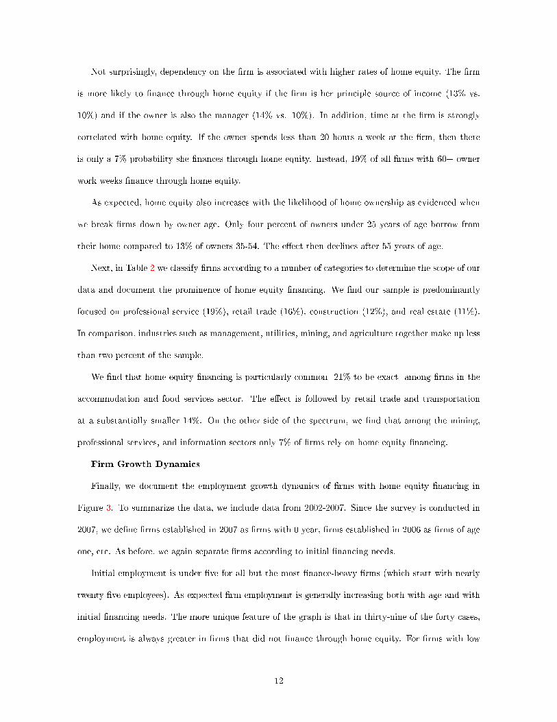
Not surprisingly, dependency on the �rm is associated with higher rates of home equity. The �rm
is more likely to �nance through home equity if the �rm is her principle source of income (13% vs.
10%) and if the owner is also the manager (14% vs. 10%). In addition, time at the �rm is strongly
correlated with home equity. If the owner spends less than 20 hours a week at the �rm, then there
is only a 7% probability she �nances through home equity. Instead, 19% of all �rms with 60+ owner
work weeks �nance through home equity.
As expected, home equity also increases with the likelihood of home ownership as evidenced when
we break �rms down by owner age. Only four percent of owners under 25 years of age borrow from
their home compared to 13% of owners 35-54. The e�ect then declines after 55 years of age.
Next, in Table 2 we classify �rms according to a number of categories to determine the scope of our
data and document the prominence of home equity �nancing. We �nd our sample is predominantly
focused on professional service (19%), retail trade (16%), construction (12%), and real estate (11%).
In comparison, industries such as management, utilities, mining, and agriculture together make up less
than two percent of the sample.
We �nd that home equity �nancing is particularly common- 21% to be exact- among �rms in the
accommodation and food services sector. The e�ect is followed by retail trade and transportation
at a substantially smaller 14%. On the other side of the spectrum, we �nd that among the mining,
professional services, and information sectors only 7% of �rms rely on home equity �nancing.
Firm Growth Dynamics
Finally, we document the employment growth dynamics of �rms with home equity �nancing in
Figure 3. To summarize the data, we include data from 2002-2007. Since the survey is conducted in
2007, we de�ne �rms established in 2007 as �rms with 0 year, �rms established in 2006 as �rms of age
one, etc. As before, we again separate �rms according to initial �nancing needs.
Initial employment is under �ve for all but the most �nance-heavy �rms (which start with nearly
twenty-�ve employees). As expected �rm employment is generally increasing both with age and with
initial �nancing needs. The more unique feature of the graph is that in thirty-nine of the forty cases,
employment is always greater in �rms that did not �nance through home equity. For �rms with low
12
�nancing needs, this e�ect is small across all ages. However, for �nance-heavy �rms, mean employment
of home-equity entrepreneurs is half the employment of �rms �nanced through alternative means.
Of course, home equity �nancing is an endogenous choice and therefore we cannot make any causal
statement linking home equity �nancing and future employment growth. To determine if home equity
loans help facilitate formal lending channels we now move to our results.
3 Results
Using our empirical speci�cation, together with the data sources discussed above, we now determine
if new �rm capital structure is driven by real estate price growth. We o�er signi�cant evidence that
a house price shock on new �rms increases home equity lending. The e�ects are greatest for �rms
with high �nancing needs. Lastly, in response to a price shock, entrepreneurs rely less on alternative
sources of �nancing, namely bank loans, family loans, and owner assets. We conclude by discussing
the policy implications of the analysis.
3.1 Estimation
Home Equity Financing
We document that local house price returns over the previous years are highly correlated with
home equity �nancing in Table 3. In our OLS regression, we �nd that a 100% increase in house prices
increases home equity by 11% among all �rms. In addition after including the local demand controls
of GDP growth and unemployment growth, the result still holds. Finally, we also estimate that a
100% increase in price results in a 4% increase in the probability a �rm �nances exclusively with home
equity.
As we have discussed, real estate price growth and �rm �nancing are likely correlated through
time-varying local demand; if GDP and unemployment are not valid proxies of local demand shocks
then this e�ect may be driving the results. Therefore, we redo the analysis by instrumenting for
exogenous real estate price growth using housing supply elasticity, and again the results hold. We note
that controlling for the state has no e�ect on our estimates given the original di�-in-di� structure. All
13
future results will depend on the instrumental variable unless otherwise mentioned.
One concern with this analysis is our lack of panel-level data, suggesting unobservable �rm �xed
e�ects might be driving the results. To overcome the concern we develop a pseudo-�rm for each state
and �nancing cohort, and then complete our analysis again in a panel regression structure1.
The holds are similar to the cross-sectional estimates as illustrated in Table 4. Increasing house
prices by 10% results in an 11% increase in home equity �nancing and a 6% increase in the chance of
�nancing entirely through home equity.
For perspective we estimate that real estate price growth between 2000 and 2006 is responsible
for a 6.3% increase in home-equity �nancing. Further, for states in the top 10% of real estate price
growth this e�ect escalates to 14%. Note, however, that our results are only an underestimate of the
true channel since we estimate the e�ect relative to �rms with minimal �nancing needs. Since these
�rms too borrow against home equity, we are understating the signi�cance of this channel.
Due to data limitations, it is slightly more di�cult to estimate the aggregate monetary increase of
home equity loans for two reasons. First, we only know whether a �rm drew on a home equity loan, not
the amount. To overcome this issue, we assume that the number of home equity loans is proportional
to the total amount of home equity �nancing; therefore if 10% of �rms depend on a home equity
loan then we assume that 10% increase of total �nancing is through this funding channel. We believe
this is actually an understatement of the true e�ect since home equity is a formal �nancing channel
when compared to family loans or credit cards. Secondly, we do not have data on the exact level of
�nancing for each �rm. Therefore as a lower bound, we assume that �rm �nancing in each cohort is
at the lower bound of the �nancing cohort; this again is an underestimate since we are substantially
under-weighting the larger �rms that are most dependent on home equity loans.
We �nd that 2000-2006 real estate price growth resulted in at least a 9% increase in the total
amount of home equity �nancing among entrepreneurs. In addition, for areas in the top 10% of house
price growth this number reaches over nineteen percent during this same period. The results highlight
the signi�cance of the home equity channel among new �rms.
1We note that due to data limitations, we identify all �rms with over $50,000 in initial �nancing in the same state asa cohort..
14
Financing Needs
In Table 5 we also check how �rm characteristics a�ects our results by completing our analysis
for each �nancing cohort. We discover that the home equity channel is greatest for �nancing needs
between $25,000 and $1 million. The e�ect actually declines slightly with the very largest �rms, which
is not surprising given that only 10% of these new businesses relied on home equity.
We �nd that a 10% increase in house prices results in a 2.1% increase in home equity �nancing
for �rms that receive between a quarter million and a million in initial funds. We redo our analysis
using the panel data and �nd only larger estimates. Again, to understand the implications, the result
suggest that 1999-2006 house price growth increased home equity �nancing by 12% in the US and up
to 27% for particularly inelastic states.
In Table 6 we simplify the analysis and compare price e�ects on �rms with the same �nancing
needs, but in di�erent states. The advantage of this framework is that we can explicitly compare �rms
with the same �nancing needs, yet subject to heterogeneous price shocks. The disadvantage is that we
can no longer compare �rms subject to the same local demand conditions. Therefore we rely especially
on our instrumental variable and local demand controls of GDP and unemployment.
We estimate that a ten percent increase in real estate value results in a three percent increase
in home equity �nancing for �rms requiring $100,000-$250,000, and a two percent increase for �rms
requiring $25,000-$100,000. The results are similar, though quantitatively smaller, when we consider
exclusively home equity �nancing.
Alternative Financing
After clearly establishing the e�ect of real estate shocks on home equity, we next consider the
impact on alternative �nancing opportunities. The results imply that in response to house price shock,
�rms take home equity loans over more expensive forms of formal debt. In comparison, other forms
of �nancing such as credit cards and savings are only minimally a�ected by real estate shocks. As a
result, we see little e�ect on the total capital structure of the �rm. As shown in Table 7 bank loans
decline by 1.7% subject to a 10% decline in real estate prices, which more than o�sets the home equity
15
a�ect. To develop a better understanding of the mechanism, in the �rst Panel of Table 8 we sort by
�nancing needs. Subject to a real estate shock all business loans �nancing decreases regardless of �rm
type, but is largest for �rms in the $250,000-$1 million range at 3.5%.
Contrast these results to alternative lending markets: we estimate no signi�cant e�ect on credit
cards lending, even when we break the sample by �nancing needs. Next, a ten percent increase in house
prices results in a 0.13% decline in family loans. The e�ect is largest for �rms in the $25,000-$50,000
range at 0.38%. In unreported results, we �nd similar estimates from the pseudo-panel methodology.
One policy implication from this work is the role of governmental loan guarantee programs. Implic-
itly, these loans should have the greatest impact when the entrepreneur has limited access to collateral,
such as when house prices are low2. Alternatively, if loan guarantee programs are una�ected by hous-
ing shocks, then entrepreneurs are either unable or uninterested to access the support exactly when it
is most valuable.
Our analysis supports the intuition that real estate price are negatively correlated with loan guar-
antee �nancing. According to Table 8 doubling house prices decreases the number of new guaranteed
loans by 1.2%. This number di�ers signi�cantly by the �nancing needs of the �rm: for �rms that
require $100,000-$250,000 in funding, this same house price shock decreases the loan quantity by three
percent.
Industry E�ects
Previous research suggest that industry could potentially drive capital structure decisions. First, pre-
vious research has found signi�cant variation in asset redeployability at the industry level: industries
with redeployable assets may be able secure debt with non-housing collateral Campello [2014], Ben-
melech et al. [2005]. Secondly, certain industries may be more dependent on external �nanceRajan
[1998]. Third, Hurst and Pugsley [2011] �nd that most small �rms have no desire to grow large or
innovate and this is especially true for skilled craftsmen, lawyers, real estate agents, doctors, small
shopkeepers, and restaurant owners.
In Table 9 we separate �rms for the twelve largest industries in our data set and �nd a clear e�ect
2Lelarge et al. [2010] conducts a similar test using a quasi-experiment in a French Loan Guarantee Program
16
of house prices on home equity �nancing for all but the arts/entertainment industry. The home equity
channel is largest for transportation, accommodation and food services, and health care. However, for
ten of the twelve industries we note a comparable decline in business loans �nancing: just as before
we note the largest e�ect for transportation and health care.
There is some evidence that small �rms tilt away from family loans subject to collateral shocks in
the following industries: (i) construction, (ii) administrative and support, and (iii) arts, entertainment,
and recreation. Lastly, we �nd that home prices negatively impact credit card �nancing in only one
industry, food and accommodation services.
Evidence during the Crisis Years
Our analysis suggest that positive house prices impact new �rm capital structure mainly through an
increase in home equity �nancing and a decrease in other bank loans. These �ndings naturally lead us
to the next question: how do the results compare to years following the housing bust3? Unfortunately,
we are not able to answer the question in this framework due to data limitations. Instead we consider
indirect evidence based on aggregate data.
To understand the relative role of collateral following the Financial Crisis we break the ratio of
Noncorporate Debt-to-GDP into three subgroups: (i) long-term debt (over one year), (ii) short-term
depository bank loans (less than one year), and (iii) short-term nondepository bank loans (including
government loans, loans from other �nancial institutions, and agricultural loans). Previous evidence
from Berger and Udell [1990] �nds that 70% of all commercial and industrial long-term debt and 30-
40% of short-term loans in the United States are secured by collateral assets. More recent estimates
by Kleiner [2014] �nd even larger numbers for private �rms at 88% for long-term debt and 46% for
short-term debt. Therefore, collateral values should impact both forms of debt, though long-term
contracts in particular.
As of May 2014, long-term debt composed 68.0% of total debt, compared to 27.4% and 4.6%
3The media has long suggested the importance of this question: �It is well known that the housing bust has taken adevastating toll on American families, nearly three million of which have lost their homes to foreclosure. Less known isthe impact that the housing collapse is having on owners of small businesses, which have often relied upon home-equityborrowing to �nance the early stages of growth and development.�-Wall Street Journal, Whelan [2012]
17
for depository loans and non-depository loans, respectively. As previously noted, the debt of US
noncorporate �rms (sole proprietorships and limited partnerships) grew faster than both household
debt and corporate debt during 1997-2009 as shown in Figure 1; then following the Financial Crisis
Noncorporate Debt-to-GDP fell 14%. Similarly, in Figure 2 we �nd that long-term debt grew through
2008 before declining till the end of the data sample in 2014. There is then no evidence that secured
debt recovered following the Financial Crisis.
So could small �rms easily switch to short-term debt markets? We �nd that depository loans fell
16% between the end of 2008 and start of 2011, suggesting a contraction in the short-term lending
market. Only in 2011 did short-term lending increase, potentially alleviating the e�ect of low collateral
values on small �rm �nancing4. The result suggests that beginning in 2011 new �rm capital structure
shifted towards short-term lending and away from long-term debt. While this may be due to sluggish
growth in the housing sector, we are not able to con�rm the hypothesis in our current framework.
4 Conclusion
This purpose of this paper is to understand the relationship between real estate prices and new �rm
capital structure. We �rst summarize the range of home equity �nancing among both �rm and owner
characteristics using new US data from the Census Survey of Business Owners. We then evaluated how
real estate shocks impact capital structure in all �rms relative to businesses with minimal �nancing
needs.
According to our analysis home equity is a source of �nancing for about 15% of large start-ups
(those that received at least $50,000 in initial funding). Secondly, a house price shock does indeed
impact �nancing: in our preferred speci�cation we �nd that a 10% increase in real estate price growth
is responsible for an 1.1% increase in home equity �nancing. Surprisingly, �rms tilt �nancing away
from bank loans, yet there is little e�ect on consumer credit cards and family loans.
4Of course these results could be driven by a decline in credit demand, not credit supply. However, according to theKau�man Firm Survey we �nd that denial rate of loans increased during the crisis years between 2007 and 2009. In2007 10.4% of all entrepreneurs were denied all loan applications. This value increased to 15% in 2008 and 19% in 2009.In addition in 2007 15.4% of entrepreneurs did not apply for loans because they would be denied, compared to 17.6% in2008 and 19.4% in 2009.
18
Aggregate data following the Financial Crisis suggests the continued role of real estate prices
in explaining current new �rm capital structure decisions. In future work we plan to extend our
analysis, focusing speci�cally on the secured debt of small �rms during the Financial Crisis. Despite
the continued interest in this area of study, many questions remain to be answered.
19

References
Manuel Adelino, Antoinette Schoar, and Felipe Severino. House prices, collateral and self-employment.
Technical report, National Bureau of Economic Research, 2013.
Efraim Benmelech, Mark J Garmaise, and Tobias J Moskowitz. Do liquidation values a�ect �nancial
contracts? evidence from commercial loan contracts and zoning regulation. The Quarterly Journal
of Economics, 120(3):1121�1154, 2005.
Allen N Berger and Gregory F Udell. Collateral, loan quality and bank risk. Journal of Monetary
Economics, 25(1):21�42, 1990.
Marco Cagetti and Mariacristina De Nardi. Entrepreneurship, frictions, and wealth. Journal of political
Economy, 114(5):835�870, 2006.
Murillo Campello. Capital structure and the redeployability of tangible assets. Econometrica, 82(2):
705�30, 2014.
Thomas Chaney, David Sraer, and David Thesmar. The collateral channel: How real estate shocks
a�ect corporate investment. The American Economic Review, 102(6):2381�2409, 2012.
Stefano Corradin and Alexander Popov. House prices, home equity borrowing, and entrepreneurship*.
Review of Financial Studies, page hhv020, 2015.
Dragana Cvijanovic. Real estate prices and �rm capital structure. UNC Kenan-Flagler Research
Paper, (2013-13), 2014.
Angus Deaton. Panel data from time series of cross-sections. Journal of econometrics, 30(1):109�126,
1985.
David S Evans and Boyan Jovanovic. An estimated model of entrepreneurial choice under liquidity
constraints. The Journal of Political Economy, pages 808�827, 1989.
Oliver Hart and John Moore. Debt and seniority: An analysis of the role of hard claims in constraining
management. The American Economic Review, 85(3):567�585, 1995.
20

Erik Hurst and Annamaria Lusardi. Liquidity constraints, household wealth, and entrepreneurship.
Journal of political Economy, 112(2):319�347, 2004.
Erik Hurst and Benjamin Wild Pugsley. What do small businesses do? Brookings Papers on Economic
Activity, 43(2 (Fall)):73�142, 2011.
Kristoph Kleiner. How real estate drives the economy: An investigation of small �rm collateral shocks
on employment. 2014.
Claire Lelarge, David Sraer, and David Thesmar. Entrepreneurship and credit constraints: Evidence
from a french loan guarantee program. In International di�erences in entrepreneurship, pages 243�
273. University of Chicago Press, 2010.
Atif Mian and Amir Su�. House prices, home equity-based borrowing, and the us household leverage
crisis. American Economic Review, 101(5):2132�56, 2011.
Atif Mian, Kamalesh Rao, and Amir Su�. Household balance sheets, consumption, and the economic
slump*. The Quarterly Journal of Economics, 128(4):1687�1726, 2013.
Raghuram Rajan. Financial dependence and growth. The American Economic Review, 88(3):559�586,
1998.
Alicia M Robb and David T Robinson. The capital structure decisions of new �rms. Review of
Financial Studies, page hhs072, 2012.
Albert Saiz. The geographic determinants of housing supply. The Quarterly Journal of Economics,
125(3):1253�1296, 2010.
Martin C Schmalz, David A Sraer, and David Thesmar. Housing collateral and entrepreneurship. 2013.
Robbie Whelan. When the home bank closes. Wall Street Journal. Midwest Edition, 2012.
21
Figure
1:USCreditMarket
LiabilitiesIndex.This�gure
displaysanindex
ofthefollow
ingvariablesfrom
1995-2013:(i)USHousehold
andNonpro�t
OrganizationCreditMarket
InstrumentLiabilities/USGDP,(ii)USNon�nancialNoncorporate
BusinessCreditMarket
InstrumentLiabilities/
US
GDP,and(iii)U
SNon�nancialCorporate
BusinessCreditMarket/USGDP.Each
variableisindexed
tobe100in
the�rstquarter
of2000.Financial
data
iscollectedfrom
theFederalReserveBoard
FlowofFundsandGDPdata
isfrom
theNationalIncomeandProduct
Accounts.Asofthe�rst
quarter
of2013Household
Liabilities/GDP=
0.77,
Corporate
Liabilities/GDP=
0.54,andNoncorporate
Liabilitieswere0.24.In
comparisonin
the
�rstquarter
of2009,thesenumber
wereHousehold
Liabilities=0.94,andCorporate
Liabilities=
0.52,andNoncorporate
Liabilities/GDP=
0.28,.
22
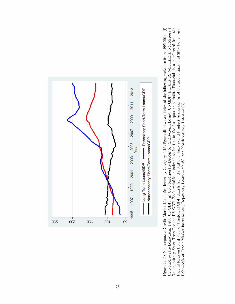
Figure
2:USNoncorporate
CreditMarket
LiabilitiesIndex
byCategory.This�gure
displaysanindex
ofthefollow
ingvariablesfrom
1995-2014:(i)
USNoncorporate
Long-Term
Debt/USGDP,(ii)USNoncorporate
Depository
Short-Term
Loans/
USGDP,and(iii)USNon�nancialNoncorporate
Nondepository
Short-Term
Loans/
USGDP.Each
variable
isindexed
tobe100in
the�rstquarter
of2000.Financialdata
iscollectedfrom
the
FederalReserve
Board
FlowofFundsandGDPdata
isfrom
theNationalIncomeandProduct
Accounts.Asofthesecondquarter
of2014Long-Term
Debt=
68%
ofCreditMarket
Instruments
,Depository
Loans=
27.4%,andNondepository
Loans=
4.6%.
23
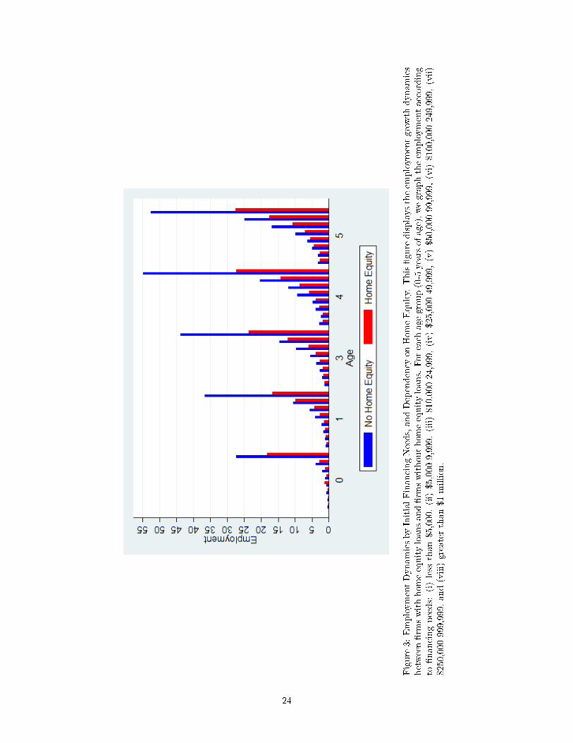
Figure
3:EmploymentDynamicsbyInitialFinancingNeeds,andDependency
onHomeEquity.
This�gure
displaystheem
ploymentgrowth
dynamics
between�rm
swithhomeequityloansand�rm
swithouthomeequityloans.Foreach
agegroup(0-5
yearsofage),wegraphtheem
ploymentaccording
to�nancingneeds:
(i)less
than$5,000,(ii)$5,000-9,999,(iii)$10,000-24,999,(iv)$25,000-49,999,(v)$50,000-99,999,(vi)$100,000-249,999,(vii)
$250,000-999,999,and(viii)greaterthan$1million.
24
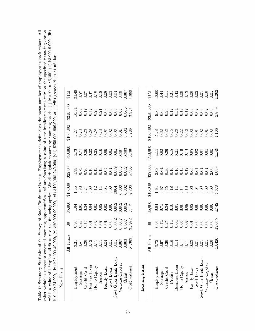
Table1:Summary
StatisticsoftheSurvey
ofSmallBusinessOwners.
Employmentisde�ned
asthemeannumber
ofem
ployees
ineach
cohort.All
other
variablesrepresentexternal�nancingopportunitiesandare
fractions;
avalueofzero
implies
no�rm
srely
onthespeci�ed
�nancingoption
whileavalueof1im
plies
all�rm
suse
the�nancingoption.Wedistinguishcohortsby�nancingneeds:
(i)less
than$5,000,(ii)$5,000-9,999,(iii)
$10,000-24,999,(iv)$25,000-49,999,(v)$50,000-99,999,(vi)$100,000-249,999,(vii)$250,000-999,999,and(viii)greaterthan$1million.
New
Firms
AllFirms
$0
$5,000
$10,000
$25,000
$50,000
$100,000
$250,000
$1M
Employment
3.21
0.90
1.04
1.55
1.99
3.73
5.27
10.34
34.49
Savings
0.81
0.88
0.85
0.80
0.73
0.71
0.70
0.69
0.57
CreditCard
0.20
0.15
0.24
0.24
0.26
0.26
0.23
0.17
0.07
BusinessLoan
0.12
0.01
0.04
0.09
0.16
0.22
0.29
0.42
0.47
HomeEquity
0.11
0.02
0.05
0.12
0.19
0.25
0.29
0.23
0.10
Assets
0.11
0.07
0.09
0.11
0.13
0.16
0.18
0.21
0.19
FamilyLoan
0.04
0.01
0.02
0.04
0.05
0.06
0.07
0.08
0.08
GovtLoan
0.01
0.00
0.00
0.00
0.01
0.01
0.02
0.03
0.03
GovtGuarBankLoan
0.01
0.0002
0.002
0004
0.009
0.01
0.03
0.06
0.04
Venture
Capital
0.007
0.0007
0.002
0.003
0.005
0.007
0.01
0.03
0.09
Grant
0.003
0.002
0.002
0.002
0.002
0.003
0.004
0.005
0.007
Observations
64,302
25,922
7,177
8,206
5,766
5,780
5,788
3,964
1,699
ExistingFirms
AllFirms
$0
$5,000
$10,000
$25,000
$50,000
$100,000
$250,000
$1M
Employment
3.72
0.96
0.94
1.64
2.03
4.11
5.18
9.80
40.60
Savings
0.67
0.74
0.71
0.67
0.64
0.62
0.62
0.60
0.44
CreditCard
0.30
0.25
0.34
0.35
0.36
0.36
0.33
0.26
0.11
Pro�ts
0.16
0.14
0.16
0.18
0.16
0.15
0.15
0.17
0.21
BusinessLoan
0.14
0.04
0.05
0.11
0.16
0.21
0.26
0.34
0.42
HomeEquity
0.11
0.03
0.06
0.11
0.15
0.19
0.22
0.19
0.09
Assets
0.11
0.07
0.09
0.10
0.12
0.14
0.16
0.17
0.13
FamilyLoan
0.03
0.01
0.02
0.03
0.05
0.05
0.06
0.06
0.06
GovtLoan
0.01
0.00
0.00
0.01
0.01
0.02
0.01
0.02
0.02
GovtGuarBankLoan
0.01
0.00
0.00
0.00
0.01
0.01
0.02
0.03
0.01
Venture
Capital
0.01
0.00
0.00
0.00
0.01
0.01
0.01
0.02
0.10
Grant
0.00
0.00
0.00
0.00
2.00
0.00
0.00
0.00
0.01
Observations
40,420
13,635
4,742
5,678
4,008
4,149
4,168
2,838
1,202
25
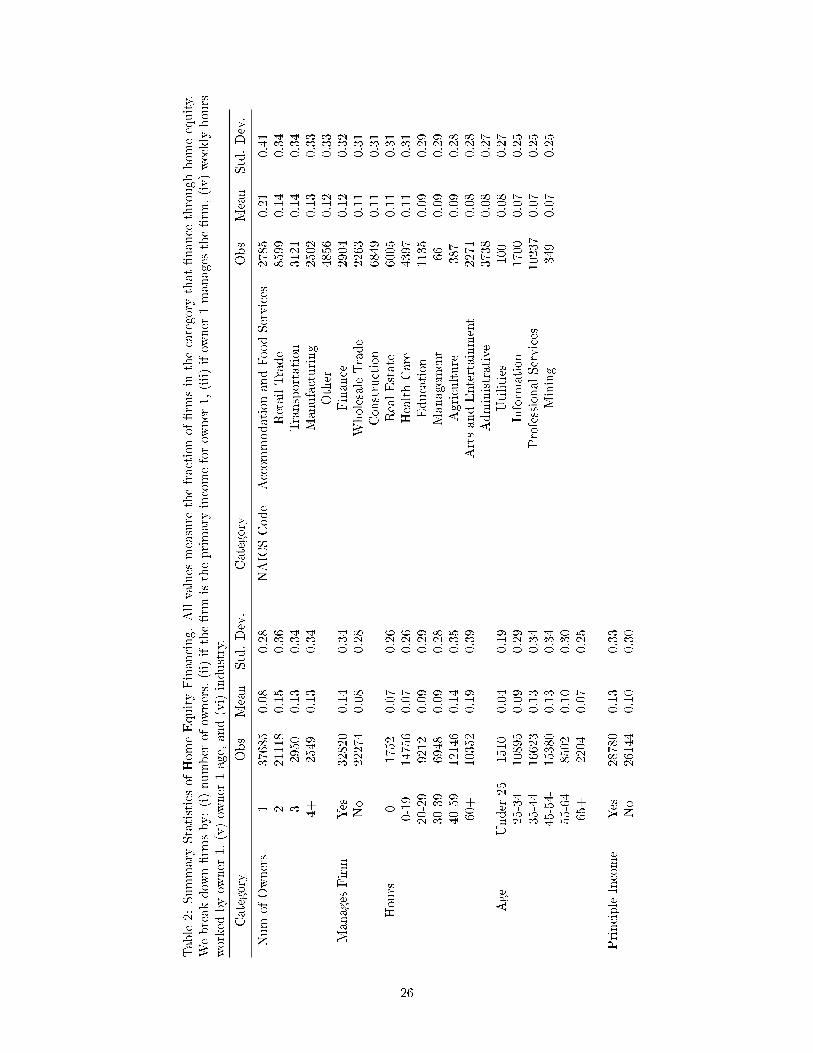
Table2:Summary
StatisticsofHomeEquityFinancing.Allvalues
measure
thefractionof�rm
sin
thecategory
that�nance
throughhomeequity.
Webreakdow
n�rm
sby:(i)number
ofow
ners,(ii)ifthe�rm
istheprimary
incomeforow
ner
1,(iii)ifow
ner
1manages
the�rm
,(iv)weekly
hours
worked
byow
ner
1,(v)ow
ner
1age,and(vi)industry.
Category
Obs
Mean
Std.Dev.
Category
Obs
Mean
Std.Dev.
Num
ofOwners
137685
0.08
0.28
NAICSCode
AccommodationandFoodServices
2785
0.21
0.41
221118
0.15
0.36
RetailTrade
8599
0.14
0.34
32950
0.13
0.34
Transportation
3121
0.14
0.34
4+
2549
0.13
0.34
Manufacturing
2502
0.13
0.33
Other
4856
0.12
0.33
Manages
Firm
Yes
32820
0.14
0.34
Finance
2904
0.12
0.32
No
22274
0.08
0.28
WholesaleTrade
2263
0.11
0.31
Construction
6849
0.11
0.31
Hours
01752
0.07
0.26
RealEstate
6005
0.11
0.31
0-19
14756
0.07
0.26
HealthCare
4397
0.11
0.31
20-29
9212
0.09
0.29
Education
1135
0.09
0.29
30-39
6948
0.09
0.28
Managem
ent
66
0.09
0.29
40-59
12146
0.14
0.35
Agriculture
387
0.09
0.28
60+
10352
0.19
0.39
ArtsandEntertainment
2271
0.08
0.28
Administrative
3738
0.08
0.27
Age
Under
25
1510
0.04
0.19
Utilities
100
0.08
0.27
25-34
10895
0.09
0.29
Inform
ation
1700
0.07
0.25
35-44
16623
0.13
0.34
ProfessionalServices
10237
0.07
0.25
45-54-
15380
0.13
0.34
Mining
349
0.07
0.25
55-64
8502
0.10
0.30
65+
2204
0.07
0.25
PrincipleIncome
Yes
28780
0.13
0.33
No
26144
0.10
0.30
26
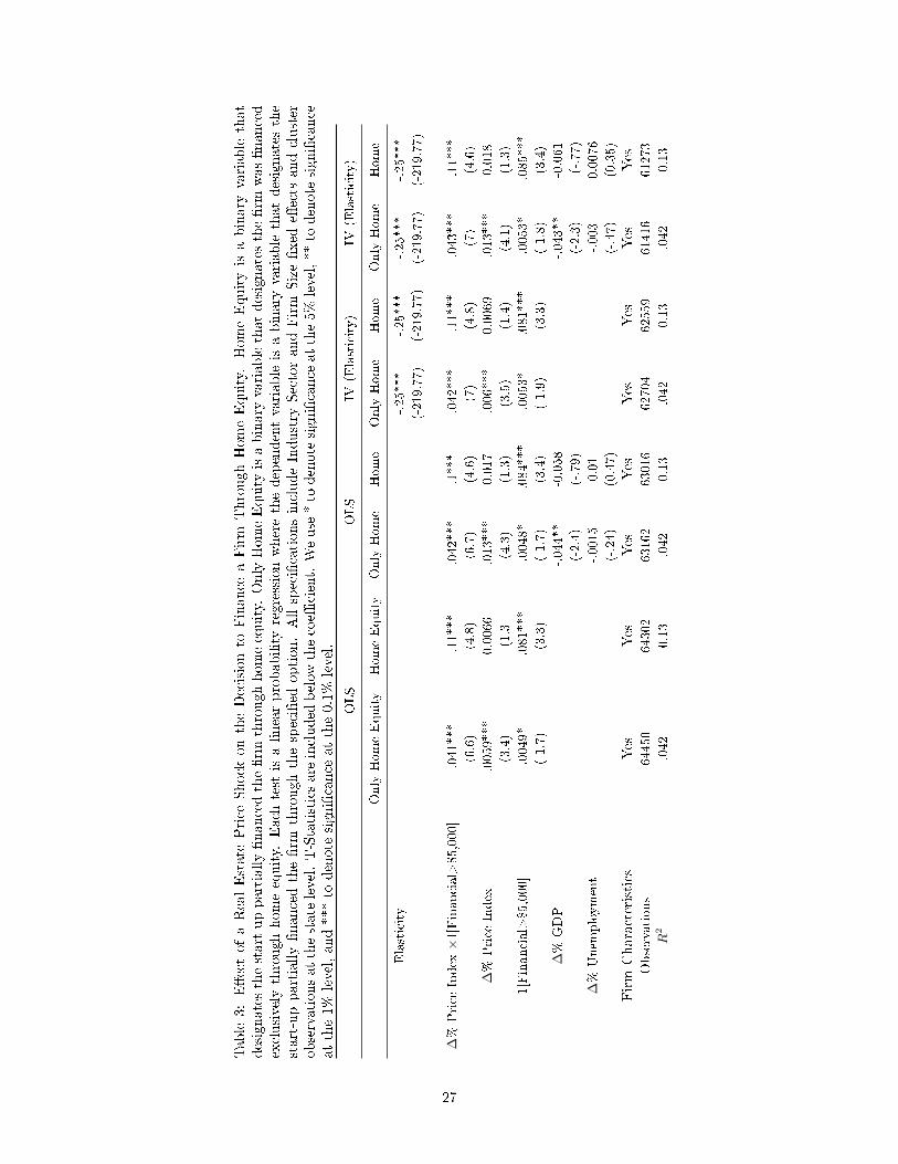
Table
3:E�ectofaRealEstate
Price
Shock
ontheDecisionto
Finance
aFirm
ThroughHomeEquity.
HomeEquityisabinary
variable
that
designatesthestart-uppartially�nancedthe�rm
throughhomeequity.
Only
HomeEquityisabinary
variablethatdesignates
the�rm
was�nanced
exclusively
through
homeequity.
Eachtest
isalinearprobabilityregressionwherethedependentvariable
isabinary
variable
thatdesignatesthe
start-uppartially�nancedthe�rm
throughthespeci�ed
option.Allspeci�cationsincludeIndustry
SectorandFirm
Size�xed
e�ects
andcluster
observationsatthestate
level.T-Statisticsare
included
below
thecoe�
cient.Weuse
*to
denote
signi�cance
atthe5%
level,**to
denote
signi�cance
atthe1%
level,and***to
denote
signi�cance
atthe0.1%
level.
OLS
OLS
IV(Elasticity)
IV(Elasticity)
Only
HomeEquity
HomeEquity
Only
Home
Home
Only
Home
Home
Only
Home
Home
Elasticity
-.25***
-.25***
-.25***
-.25***
(-219.77)
(-219.77)
(-219.77)
(-219.77)
∆%
Price
Index
×1[Financial>$5,000]
.041***
.11***
.042***
.1***
.042***
.11***
.043***
.11***
(6.6)
(4.8)
(6.7)
(4.6)
(7)
(4.8)
(7)
(4.6)
∆%
Price
Index
.0059***
0.0066
.013***
0.017
.006***
0.0069
.013***
0.018
(3.4)
(1.3
(4.3)
(1.3)
(3.5)
(1.4)
(4.1)
(1.3)
1[Financial>$5,000]
-.0049*
.081***
-.0048*
.084***
-.0053*
.081***
-.0053*
.085***
(-1.7)
(3.3)
(-1.7)
(3.4)
(-1.9)
(3.3)
(-1.8)
(3.4)
∆%
GDP
-.044**
-0.058
-.043**
-0.061
(-2.4)
(-.79)
(-2.3)
(-.77)
∆%
Unem
ployment
-.0015
0.01
-.003
0.0076
(-.24)
(0.47)
(-.47)
(0.35)
Firm
Characteristics
Yes
Yes
Yes
Yes
Yes
Yes
Yes
Yes
Observations
64450
64302
63162
63016
62704
62559
61416
61273
R2
.042
0.13
.042
0.13
.042
0.13
.042
0.13
27
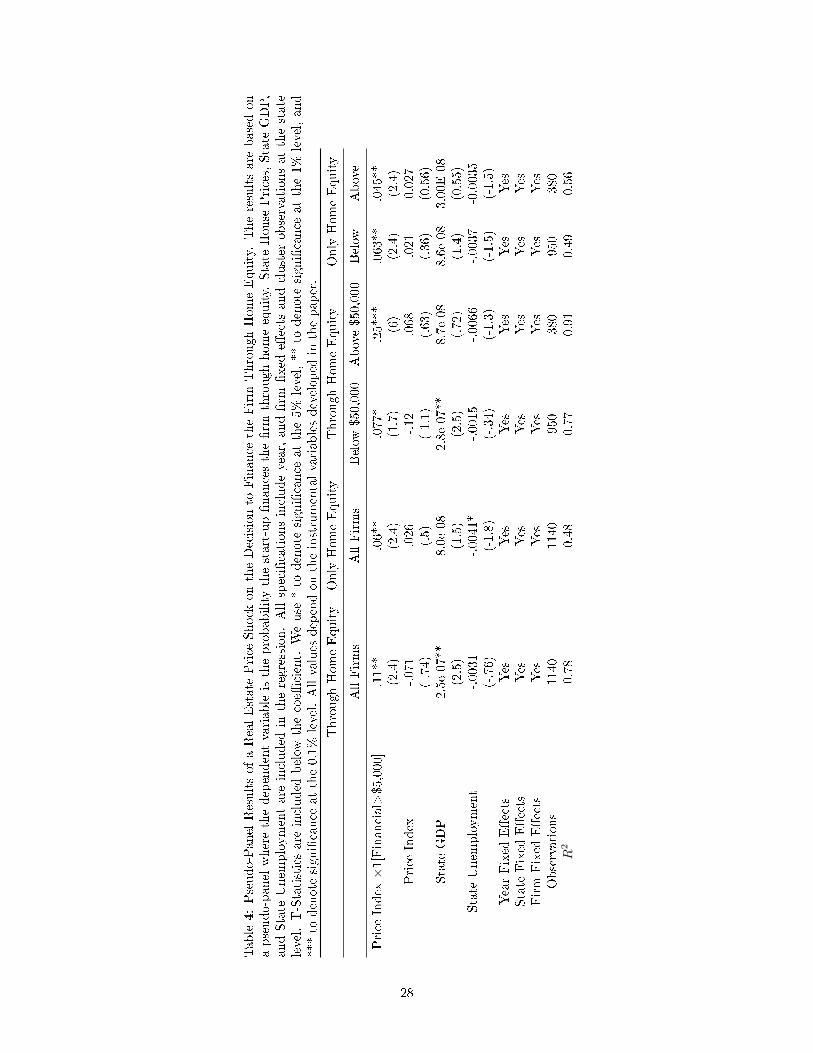
Table4:Pseudo-PanelResultsofaRealEstate
Price
Shock
ontheDecisionto
Finance
theFirm
ThroughHomeEquity.
Theresultsare
basedon
apseudo-panelwherethedependentvariableistheprobabilitythestart-up�nancesthe�rm
throughhomeequity.
State
House
Prices,State
GDP,
andState
Unem
ploymentare
included
intheregression.Allspeci�cationsincludeyear,and�rm
�xed
e�ects
andcluster
observationsatthestate
level.T-Statisticsare
included
below
thecoe�
cient.
Weuse
*to
denote
signi�cance
atthe5%
level,**to
denote
signi�cance
atthe1%
level,and
***to
denote
signi�cance
atthe0.1%
level.Allvalues
dependontheinstrumentalvariablesdeveloped
inthepaper.
ThroughHomeEquity
Only
HomeEquity
ThroughHomeEquity
Only
HomeEquity
AllFirms
AllFirms
Below
$50,000
Above$50,000
Below
Above
Price
Index
×1[Financial>$5,000]
.11**
.06**
.077*
.25***
.063**
.045**
(2.4)
(2.4)
(1.7)
(6)
(2.4)
(2.4)
Price
Index
-.071
.026
-.12
.068
.021
0.027
(-.74)
(.5)
(-1.1)
(.63)
(.36)
(0.56)
State
GDP
2.5e-07**
8.0e-08
2.8e-07**
8.7e-08
8.6e-08
3.00E-08
(2.5)
(1.5)
(2.5)
(.72)
(1.4)
(0.55)
State
Unem
ployment
-.0031
-.0041*
-.0015
-.0066
-.0037
-0.0035
(-.76)
(-1.8)
(-.34)
(-1.3)
(-1.5)
(-1.5)
YearFixed
E�ects
Yes
Yes
Yes
Yes
Yes
Yes
State
Fixed
E�ects
Yes
Yes
Yes
Yes
Yes
Yes
Firm
Fixed
E�ects
Yes
Yes
Yes
Yes
Yes
Yes
Observations
1140
1140
950
380
950
380
R2
0.78
0.48
0.77
0.91
0.49
0.56
28
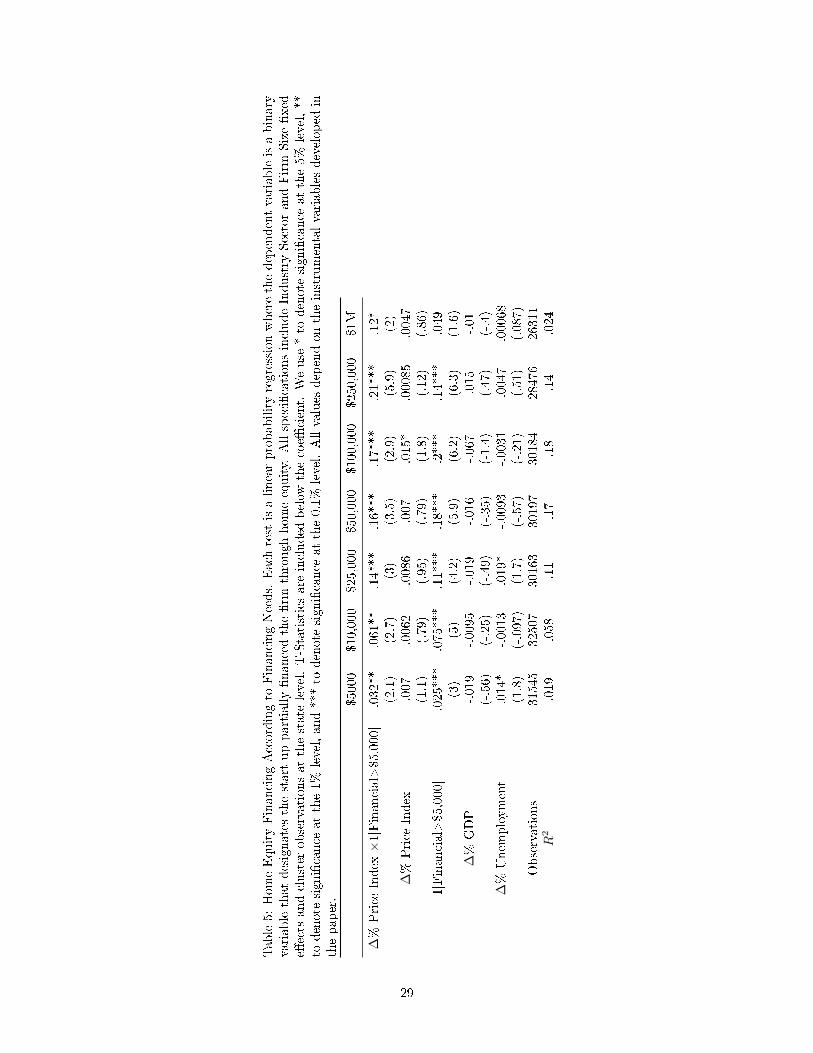
Table5:HomeEquityFinancingAccordingto
FinancingNeeds.
Each
test
isalinearprobabilityregressionwherethedependentvariableisabinary
variablethatdesignatesthestart-uppartially�nancedthe�rm
throughhomeequity.
Allspeci�cationsincludeIndustry
SectorandFirm
Size�xed
e�ects
andcluster
observationsatthestate
level.T-Statisticsare
included
below
thecoe�
cient.
Weuse
*to
denote
signi�cance
atthe5%
level,**
todenote
signi�cance
atthe1%
level,and***to
denote
signi�cance
atthe0.1%
level.Allvalues
dependontheinstrumentalvariablesdeveloped
inthepaper.
$5000
$10,000
$25,000
$50,000
$100,000
$250,000
$1M
∆%
Price
Index
×1[Financial>$5,000]
.032**
.061**
.14***
.16***
.17***
.21***
.12*
(2.1)
(2.7)
(3)
(3.5)
(2.9)
(5.9)
(2)
∆%
Price
Index
.007
.0062
.0086
.007
.015*
.00085
.0047
(1.1)
(.79)
(.95)
(.79)
(1.8)
(.12)
(.86)
1[Financial>$5,000]
.025***
.075***
.11***
.18***
.2***
.14***
.049
(3)
(5)
(4.2)
(5.9)
(6.2)
(6.3)
(1.6)
∆%
GDP
-.019
-.0095
-.019
-.016
-.067
.015
-.01
(-.56)
(-.25)
(-.49)
(-.35)
(-1.4)
(.47)
(-.4)
∆%
Unem
ployment
.014*
-.0013
.019*
-.0093
-.0031
.0047
.00068
(1.8)
(-.097)
(1.7)
(-.57)
(-.21)
(.51)
(.087)
Observations
31545
32507
30163
30197
30184
28476
26311
R2
.019
.058
.11
.17
.18
.14
.024
29
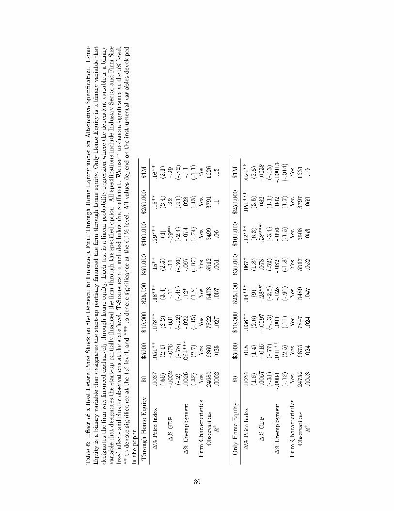
Table
6:E�ectofaRealEstate
Price
Shock
ontheDecisionto
Finance
aFirm
ThroughHomeEquityunder
anAlternative
Speci�cation.Home
Equityisabinary
variablethatdesignatesthestart-uppartially�nancedthe�rm
throughhomeequity.
Only
HomeEquityisabinary
variablethat
designatesthe�rm
was�nancedexclusivelythroughhomeequity.
Each
testisalinearprobabilityregressionwherethedependentvariableisabinary
variablethatdesignatesthestart-uppartially�nancedthe�rm
throughthespeci�ed
option.Allspeci�cationsincludeIndustry
SectorandFirm
Size
�xed
e�ectsandcluster
observationsatthestate
level.T-Statisticsare
included
below
thecoe�
cient.Weuse
*to
denote
signi�cance
atthe5%
level,
**to
denote
signi�cance
atthe1%
level,and***to
denote
signi�cance
atthe0.1%
level.Allvalues
dependontheinstrumentalvariablesdeveloped
inthepaper.
ThroughHomeEquity
$0
$5000
$10,000
$25,000
$50,000
$100,000
$250,000
$1M
∆%
Price
Index
.0037
.051**
.078**
.18***
.18**
.29***
.15**
.16**
(.66)
(2.4)
(2.2)
(3.4)
(2.5)
(4)
(2.4)
(2.1)
∆%
GDP
-.0052
-.076
-.031
-.11
-.11
-.69**
.22
-.29
(-.2)
(-.78)
(-.22)
(-.46)
(-.36)
(-2.4)
(.91)
(-.82)
∆%
Unem
ployment
.0026
.064***
-.022
.12*
-.097
-.074
.028
-.11
(.32)
(2.7)
(-.45)
(1.8)
(-.97)
(-.74)
(.43)
(-1.1)
Firm
Characteristics
Yes
Yes
Yes
Yes
Yes
Yes
Yes
Yes
Observations
24685
6860
7822
5478
5512
5499
3791
1626
R2
.0062
.025
.027
.057
.051
.06
.1.12
Only
HomeEquity
$0
$5000
$10,000
$25,000
$50,000
$100,000
$250,000
$1M
∆%
Price
Index
.0054
.018
.036**
.14***
.067*
.12***
.051***
.024**
(1.6)
(1.4)
(2.6)
(9)
(1.8)
(6.3)
(3.5)
(2.6)
∆%
GDP
-.0067
-.046
-.0097
-.28**
.078
-.38***
.082
-.0038
(-.31)
(-.77)
(-.13)
(-2.5)
(.52)
(-3.4)
(1.1)
(-.13)
∆%
Unem
ployment
-.00041
.041**
.004
-.028
-.082*
-.056
.042
-.00013
(-.12)
(2.5)
(.14)
(-.91)
(-1.8)
(-1.5)
(1.7)
(-.014)
Firm
Characteristics
Yes
Yes
Yes
Yes
Yes
Yes
Yes
Yes
Observations
24752
6875
7847
5489
5517
5508
3797
1631
R2
.0058
.024
.024
.047
.052
.053
.069
.19
30
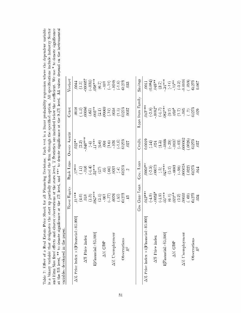
Table
7:E�ectofaRealEstate
Price
Shock
forallFinancingDecisions.
Each
test
isalinearprobabilityregressionwherethedependentvariable
isabinary
variablethatdesignatesthestart-uppartially�nancedthe�rm
through
thespeci�ed
option.Allspeci�cationsincludeIndustry
Sector
andFirm
Size�xed
e�ects
andcluster
observationsatthestate
level.T-Statisticsare
included
below
thecoe�
cient.
Weuse
*to
denote
signi�cance
atthe5%
level,**to
denote
signi�cance
atthe1%
level,and***to
denote
signi�cance
atthe0.1%
level.Allvalues
dependontheinstrumental
variablesdeveloped
inthepaper.
HomeEquity
BankLoan
Owner
Assets
Grant
Venture
∆%
Price
Index
×1[Financial>$5,000]
.11***
-.17***
.022**
-.0018
.0044
(4.6)
(-11)
(2.2)
(-1.1)
(1.5)
∆%
Price
Index
.018
-.016
-.046***
.00086
-000037
(1.3)
(-1.4)
(-4)
(.65)
(-.031)
1[Financial>$5,000]
.085***
.52***
.11***
.003**
.058***
(3.4)
(17)
(6.6)
(2.1)
(6.7)
∆%
GDP
-.061
.05
.068
.00069
-.001
(-.77)
(.66)
(1.6)
(.12)
(-.14)
∆%
Unem
ployment
.0076
.0091
-.026
.0034
-.0048
(.35)
(.4)
(-1.6)
(1.5)
(-1.6)
Observations
61273
61273
61273
61273
61273
R2
.13
.2.027
.0037
.033
Gov
Guar
Loan
Gov.Loan
Credit
Loanfrom
Family
Savings
∆%
Price
Index
×1[Financial>$5,000]
-.012***
-.0068**
0.0019
-.013***
.0011
(-4.9)
(-2.5)
(.14)
(-2.8)
(0.084)
∆%
Price
Index
-.0033*
.00073
.024
-.0092*
.045**
(-1.9)
(.5)
(1.3)
(-1.7)
(2.7)
1[Financial>$5,000]
.05***
.027***
-.0066
.083***
-.34***
(6.4)
(5.2)
(-.39)
(9.2)
(-14)
∆%
GDP
.022**
-.0083
-.0027
.059*
-.15**
(2.2)
(-.98)
(-.03)
(1.7)
(-2.2)
∆%
Unem
ployment
.00031
.000078
.000062
-.005
-0.0016
(.-69)
(.022)
(.0026)
(-.7)
(-.059)
Observations
61273
61273
61273
61273
61273
R2
.031
.014
.037
.029
0.067
31
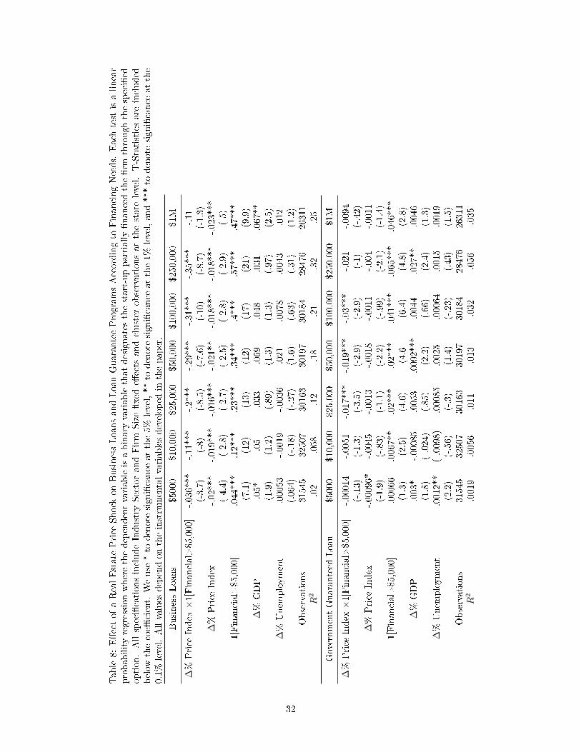
Table8:E�ectofaRealEstate
Price
Shock
onBusinessLoansandLoanGuaranteeProgramsAccordingto
FinancingNeeds.
Each
test
isalinear
probabilityregressionwherethedependentvariableisabinary
variablethatdesignatesthestart-uppartially�nancedthe�rm
throughthespeci�ed
option.Allspeci�cationsincludeIndustry
SectorandFirm
Size�xed
e�ects
andcluster
observationsatthestate
level.T-Statisticsare
included
below
thecoe�
cient.
Weuse
*to
denote
signi�cance
atthe5%
level,**to
denote
signi�cance
atthe1%
level,and***to
denote
signi�cance
atthe
0.1%
level.Allvalues
dependontheinstrumentalvariablesdeveloped
inthepaper.
BusinessLoans
$5000
$10,000
$25,000
$50,000
$100,000
$250,000
$1M
∆%
Price
Index
×1[Financial>$5,000]
-.036***
-.11***
-.2***
-.29***
-.31***
-.35***
-.11
(-3.7)
(-8)
(-8.5)
(-7.6)
(-10)
(-8.7)
(-1.3)
∆%
Price
Index
-.02***
-.019***
-.016***
-.021**
-.018***
-.018***
-.023***
(-4.4)
(-2.8)
(-2.7)
(-2.5)
(-2.8)
(-2.9)
(-5)
1[Financial>$5,000]
.044***
.12***
.23***
.34***
.4***
.57***
.47***
(7.1)
(12)
(13)
(12)
(17)
(21)
(9.9)
∆%
GDP
.05*
.05
.033
.069
.048
.031
.067**
(1.9)
(1.2)
(.89)
(1.3)
(1.3)
(.97)
(2.5)
∆%
Unem
ployment
.00053
-.0019
-.0036
.021
.0078
.0043
.012
(.064)
(-.18)
(-.27)
(1.6)
(.63)
(.31)
(1.2)
Observations
31545
32507
30163
30197
30184
28476
26311
R2
.02
.058
.12
.18
.21
.32
.25
GovernmentGuaranteed
Loan
$5000
$10,000
$25,000
$50,000
$100,000
$250,000
$1M
∆%
Price
Index
×1[Financial>$5,000]
-.00014
-.0051
-.017***
-.019***
-.03***
-.021
-.0094
(-.13)
(-1.3)
(-3.5)
(-2.9)
(-2.9)
(-1)
(-.42)
∆%
Price
Index
-.00096*
-.0045
-.0013
-.0018
-.0011
-.004
-.0011
(-1.9)
(-.83)
(-1.1)
(-2.2)
(-.99)
(-2.1)
(-1.4)
1[Financial>$5,000]
.00066
.0067**
.02***
.02***
.041***
.065***
.046***
(1.3)
(2.5)
(4.6)
(4.6
(6.4)
(4.8)
(2.8)
∆%
GDP
.003*
-.00085
.0053
.0092***
.0044
.027**
.0046
(1.8)
(-.024)
(.85)
(2.2)
(.66)
(2.4)
(1.3)
∆%
Unem
ployment
.0012**
(-.0098)
-.00085
.0025
-.00064
.0015
.0019
(2.2)
(-.56)
(-.3)
(1.4)
(-.23)
(.43)
(1.5)
Observations
31545
32507
30163
30197
30184
28476
26311
R2
.0019
.0056
.011
.013
.032
.056
.035
32
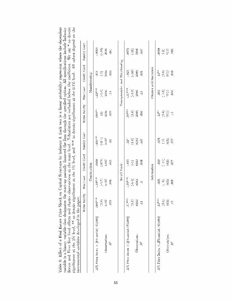
Table
9:E�ectofaRealEstate
Price
Shock
onCapitalStructure
byIndustry
I.Each
test
isalinearprobabilityregressionwherethedependent
variableisabinary
variablethatdesignatesthestart-uppartially�nancedthe�rm
throughthespeci�ed
option.Allspeci�cationsincludeIndustry
SectorandFirm
Size�xed
e�ects
andcluster
observationsatthestate
level.
T-Statisticsare
included
below
thecoe�
cient.
Weuse
*to
denote
signi�cance
atthe5%
level,**to
denote
signi�cance
atthe1%
level,and***to
denote
signi�cance
atthe0.1%
level.Allvalues
dependonthe
instrumentalvariablesdeveloped
inthepaper.
HomeEquity
BusLoan
CreditCard
FamilyLoan
HomeEquity
BusLoan
CreditCard
FamilyLoan
Construction
Manufacturing
∆%
Price
Index×1[Financial>$5,000]
.098***
-.19***
.0038
-.031**
.084**
-.22***
.051
-.0054
(2.8)
(-5.7)
(.074)
(-2.4)
(2)
(-5.4)
(.5)
(-.16)
Observations
6437
6437
6437
6437
2346
2346
2346
2346
R2
.079
.096
.045
.03
.079
.14
.053
.061
RetailTrade
TransportationandWarehousing
∆%
Price
Index×1[Financial>$5,000]
.11***
-.15***
-.041
.02*
.18***
-.31***
-.025
.0072
(3.1)
(-6.4)
(-1)
(1.8)
(3.4)
(-3.9)
(-.38)
(.31)
Observations
8163
8163
8163
8163
2966
2966
2966
2966
R2
.11
.1.034
.037
.095
.13
.031
.037
Inform
ation
Finance
andInsurance
∆%
Price
Index×1[Financial>$5,000]
.12***
-.025
-.018
-.028
.12**
-.052
.12**
.0098
(3.5)
(-.6)
(-.17)
(-1)
(2.4)
(-1.6)
(2.6)
(.3)
Observations
1635
1635
1635
1635
2777
2777
2777
2777
R2
.12
.068
.077
.077
.11
.056
.059
.035
33
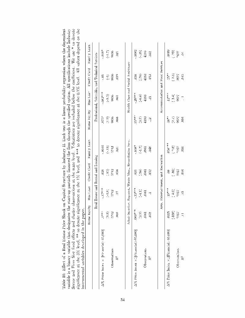
Table10:E�ectofaRealEstate
Price
Shock
onCapitalStructure
byIndustry
II.Each
test
isalinearprobabilityregressionwherethedependent
variableisabinary
variablethatdesignatesthestart-uppartially�nancedthe�rm
throughthespeci�ed
option.Allspeci�cationsincludeIndustry
SectorandFirm
Size�xed
e�ects
andcluster
observationsatthestate
level.
T-Statisticsare
included
below
thecoe�
cient.
Weuse
*to
denote
signi�cance
atthe5%
level,**to
denote
signi�cance
atthe1%
level,and***to
denote
signi�cance
atthe0.1%
level.Allvalues
dependonthe
instrumentalvariablesdeveloped
inthepaper.
HomeEquity
BusLoan
CreditCard
FamilyLoan
HomeEquity
BusLoan
CreditCard
FamilyLoan
RealEstate
andRentalandLeasing
Professional,Scienti�c,andTechnicalServices
∆%
Price
Index×1[Financial>$5,000]
.1***
-.17***
.028
-.0016
.075*
-.082***
-.03
-.018*
(3.3)
(-4.9)
(.85)
(-.13)
(1.9)
(-3.5)
(-1)
(-1.7)
Observations
5742
5742
5742
5742
9836
9836
9836
9836
R2
.069
.17
.058
.024
.068
.061
.039
.021
Administrative,Support,WasteMan.,Rem
ediationServ.
HealthCare
andSocialAssistance
∆%
Price
Index×1[Financial>$5,000]
.089***
-.13***
.031
-.038*
.15***
-.25***
.038
-.0082
(3.9)
(-4.1)
(.58)
(-1.7)
(3.7)
(-6.8)
(.76)
(-.35)
Observations
3561
3561
3561
3561
4193
4193
4193
4193
R2
.078
.1.052
.048
.12
.21
.053
.032
Arts,Entertainment,andRecreation
AccommodationandFoodServices
∆%
Price
Index×1[Financial>$5,000]
.0025
-.19***
-.08
-.058***
.16**
-.12***
-.25**
-.0089
(.038)
(-4.9)
(-.89)
(-2.8)
(2.7)
(-3.4)
(-2.5)
(-.29)
Observations
2167
2167
2167
2167
2627
2627
2627
2627
R2
.11
.13
.056
.036
.094
.11
.045
.04
34