House Prices and Consumer Spending ∗

David Berger

Northwestern University

Veronica Guerrieri

University of Chicago

Guido Lorenzoni

Northwestern University

Joseph Vavra

University of Chicago

October 28, 2015

Abstract

Recent empirical work shows large consumption responses to house price movements.

Can consumption theory explain these responses? We consider a variety of consumption

models with uninsurable income risk and show that consumption responses to permanent

house price shocks can be approximated by a simple “sufficient-statistic” formula: the

marginal propensity to consume out of temporary income times the value of housing.

Calibrated versions of the models generate house price effects that are both large and

sensitive to the level of household debt in the economy. We apply our formula to micro

data to provide a new measure of house price effects.

Keywords: Consumption, House Prices, MPC, Leverage, Debt, State-Dependence.

JEL Codes: E21, E32, E6, D14, D91, R21.

∗Email: Berger: david.berger@northwestern.edu; Guerrieri: vguerrie@chicagobooth.edu; Lorenzoni:guido.lorenzoni@northwestern.edu; Vavra: joseph.vavra@chicagobooth.edu. We thank Sasha Indarte and DavidArgente for excellent research assistance. We would also like to thank Orazio Attanasio, Adrien Auclert, JoaoCocco, Jonathan Parker, Monika Piazzesi, Martin Schneider, Alp Simsek, Chris Tonetti, Gianluca Violanteand seminar participants at Brown, Cambridge CFM, CSEF-CIM-UCL Workshop, Empirical Macro Workshop-Austin, Maryland, Northwestern, Penn State, SED-Warsaw, EIEF, SITE, Stanford, LSE, LBS, Bocconi, BostonFed, and Booth.

1 Introduction

The last recession in the US was characterized by a large and persistent decline in consumer

spending.1 Many observers have pointed to the evolution of house prices and household debt as

important factors in explaining consumption dynamics before and during the recession. More

broadly, there is a widespread policy concern that boom-busts cycles in housing and consumer

debt can end with large contractions in consumer spending.2 A growing empirical literature

argues that consumption responds strongly to house price movements, thus suggesting an im-

portant role for housing wealth in consumption dynamics. However, the theoretical rationale

for these house price effects on consumption is less clear. In particular, it is a commonly held

view that house price effects on consumption should be small, because for most households an

increase in the price of their house is associated with an equivalent increase in expected future

implicit rental costs.3 What models can deliver the large effects found in the empirical litera-

ture and what are the mechanisms at work? Are house price effects larger when the household

sector is more levered? Is it important that housing can be used as collateral? Can house

price movements independently lead to large consumption swings or do they require correlated

movements in common factors such as income or financial conditions?

In this paper, we study these questions in the context of a fairly standard class of incom-

plete market models with income uncertainty and housing that serves as collateral. Our main

quantitative conclusions are: (i) Reasonable calibrations of this class of models can produce

large consumption responses to exogenous house price changes, in line with the recent empirical

literature; (ii) The size of these responses depends crucially on initial conditions in the economy,

namely, on the initial joint distribution of housing and debt.

In the process of delivering these quantitative conclusions, we derive a theoretical result

which sheds light on the mechanism behind these findings. We show that in our baseline

model, the individual response of consumption to an unexpected, permanent house price change

is given by a simple “sufficient-statistic” formula: the individual marginal propensity to con-

sume out of temporary income shocks (MPC) times individual housing values. The aggregate

response is then determined by the endogenous joint distribution of the MPC and housing.

This formula helps explain why different versions of our model, which produce different joint

distributions, generate different average responses. It also explains why, following different his-

tories of past shocks, which produce different initial conditions, an economy displays different

aggregate responses to current shocks.

Our formula implies that the total consumption response to a change in house prices can

be interpreted as a pure “endowment effect” driven by the change in value of initial housing

1See Petev et al. (2012).2See Cerutti et al. (2015).3See the literature discussed below.

1

endowments. However, this result should be interpreted with care, as it does not imply that

other effects are not at work. Higher house prices increase the value of housing endowments, but

also induce income and substitution effects as the relative price of housing services increases,

and they relax borrowing constraints through a collateral channel. We analyze these effects

and show that each one is large when viewed in isolation. However, if one is interested in

understanding the total effect, these four channels are tightly linked together: in our baseline

model the income, substitution and collateral effects cancel out, so that only the endowment

effect remains.

Our baseline is a partial equilibrium model calibrated to life-cycle wealth data from the

Survey of Consumer Finances. We show that this model delivers an average elasticity of con-

sumption to house price shocks over working life of 0.47. Two model features explain this

relatively large elasticity. First, with income uncertainty and precautionary savings, the con-

sumption function is concave in net-worth so that low net-worth agents have large MPCs.

Second, housing services enter the utility function, which implies that housing wealth is not

proportional to total net-worth. In particular, low net-worth agents choose to borrow and thus

hold housing that is a multiple of net worth. Therefore, the model generates a joint distribution

with a sizable mass of households at high housing levels and, at the same time, low net worth

and high MPC. Using our formula, this implies that the aggregate consumption response to

house price shocks is large. Thus, relatively standard models imply large responses of consump-

tion to pure changes in house prices and do not require additional features such as house price

movements which are correlated with future income in order to generate these effects.

The baseline model features no transaction costs in housing and no rental option. Therefore,

it produces an unrealistic frequency of house trading and cannot match the large fraction of

renters in the population, so we extend the model to allow for illiquid housing and rentals. In

the extended model, our sufficient-statistic formula no longer holds exactly, but we show that

for realistic parameter choices it still provides a good approximation. Somewhat surprisingly,

the presence of housing adjustment costs has only minor quantitative implications for the effect

of house prices on consumption. The main quantitative difference between the baseline and

the extended model comes from the presence of renters. In the model with renters the average

response over working life is smaller and equal to 0.24. This is due not only to the fact that

some agents do not own a house, and thus have a zero endowment effect, but also to the fact

that agents who choose to rent are precisely the low net-worth, high-MPC agents who would

display the biggest responses if they owned.

After showing that the sufficient-statistic approximation is robust to various model spec-

ifications, we take our formula directly to consumption data. Estimating the distribution of

MPC × PH in the data (where PH denotes house values) provides an alternative sufficient-

statistic-based measure of housing price effects and can also be interpreted as a test of our

2

structural consumption model. The main challenge is to estimate MPCs conditional on hous-

ing holdings, which we address by extending the approach of Blundell, Pistaferri and Preston

(2008) to recent PSID data. We find that the micro patterns of MPC × PH are similar to

those implied by our simulations and that our sufficient-statistic-based measure of housing price

effects is in line with existing estimates.

The majority of our paper focuses on the consumption response to one-time, permanent

house price shocks. In the final section of the paper we extend the analysis to dynamics,

focusing on a boom-bust housing cycle. A typical feature of housing cycles is that residential

investment first increases and then decreases, along with house prices, suggesting an important

role for shifts in housing demand. In order to generate such shifts, we introduce changes in

expected future house price growth. We show that these changes in expected growth allow us

to match the cyclical behavior of residential investment. At the same time, changes in expected

growth have only mild direct effects on consumption, so consumption is primarily driven by

the house price effect investigated in the rest of the paper.4 However, this does not imply that

shifts in housing demand are irrelevant for consumption dynamics. The important channel

here is that past shifts in housing demand affect the joint distribution of housing and debt, and

thus determine the magnitude of the house price effect. In particular, in our simulations, the

increase in housing demand during the boom leads to increased leverage, and this contributes

substantially to the consumption contraction caused in the bust.

The boom-bust simulations show that the distribution of housing and debt matters for

the strength of house price effects. This observation is important when interpreting empirical

evidence from different time periods and when contemplating potential policy intervention into

housing markets. Both shocks and policy interventions may have effects on consumption that

differ dramatically depending on the distribution of states at the time the policy is enacted.

In this sense, our result joins a growing literature arguing that the economy may exhibit time-

varying responses to aggregate shocks.5

Our paper is motivated by the empirical literature studying house price effects on consump-

tion. While methodological and data differences have led to a wide range of estimates for the

relationship between house prices and consumption, the literature has generally found strong

relationships. Whether or not such relationships are causal is more contentious, but recent

papers with new sources of identification have argued for large effects.6 We contribute to this

debate both by showing that theory is consistent with large causal effects and by constructing

4These results also show that our quantitative conclusions are robust to relaxing the assumption of permanentshocks.

5See e.g. Berger and Vavra (2015) for applications to durable goods, Vavra (2014) for applications to pricesand Caballero and Engel (1999) and Winberry (2015) for applications to investment.

6While there are different ways of measuring housing price effects, for consistency we will focus the discussionon estimates of the consumption elasticity to house prices—the percentage change in non-durable consumptiondue to a one percent change in house prices.

3

a new sufficient-statistic based measure of housing price effects.

In two influential studies using aggregate data, Case et al. (2013) find elasticities from 0.03

to 0.18, with most of the their estimates centered around 0.10, while Carroll et al. (2011) find

an immediate (next-quarter) elasticity of 0.047, with an eventual elasticity of around 0.20.7

There are also a number of studies that exploit household level micro data, which allows for

substantially more variation in consumption and house prices and for alternative sources of

identification. Such studies have led to a wide range of estimates. For example, Campbell and

Cocco (2007) find an average elasticity of non-durable consumption to house prices of about 1.2

with larger results for old homeowners than for young homeowners. In contrast, Attanasio et al.

(2009) find that the average non-durable consumption elasticity is 0.15 and that consumption

response of young homeowners is much stronger than it is for old homeowners.

The greatest challenge for these studies is that it is hard to find exogenous variation in

house prices which can be used to separate direct house price effects from the effects of common

factors. In particular, an important concern is that expectations about future income growth

may drive both house prices and consumption.8 Mian et al. (2013) make progress on this front by

using high quality credit card data together with the Saiz (2010) housing supply instrument to

isolate the effects of exogenous changes in house prices on highly localized measures of spending.

Their baseline estimates of the non-durable consumption elasticity are between 0.13 and 0.26.9

Although these estimates can be interpreted as consumption responses to exogenous house price

shocks, it is important to note that they are not pure partial equilibrium responses, since they

reflect both direct house price effects plus any local general equilibrium responses. In particular,

they include the additional effect on consumption due to increases in local incomes driven by

greater non-tradable spending. Despite this caveat, we nevertheless view the elasticities from

Mian et al. (2013) as the closest empirical analogue to the direct house price effects in our

theory, so we will often compare our theoretical results to these numbers. Several recent papers

such as Kaplan et al. (2015) and Stroebel and Vavra (2015) also arrive at similar numbers using

new scanner spending data and additional identification strategies.

Throughout the paper, we refer to a commonly held view that house price effects should

be small in standard consumption models. One of the clearest formulations of this view is

in Sinai and Souleles (2005) (p. 773), who argue that “increases in house prices reflect a

commensurate increase in the present value of expected future rents” and “for homeowners

7They report results in terms of MPCs of 2 and 9 cents (in 2007 dollars) respectively. In 2007, housingassets from the Flow of Funds were $28,369 billion and personal consumption expenditures from the BEA were$9,750.5 billion. This delivers the reported elasticities.

8See Attanasio and Weber (1994).9They report estimates between 0.5-0.8. However, given their methodology these estimates need to be scaled

by housing wealth/total wealth to be comparable to the other estimates listed above. Since the mean housingwealth to total wealth ratio in their data is between 0.25-0.33, this implies elasticity estimates ranging from0.13 to 0.26.

4

with infinite horizons, this increase in implicit liabilities would exactly offset the increase in the

house value, leaving their effective expected net worth unchanged.”10 To clarify the connection

with this line of argument, we begin our analysis from a special case with no income risk where

the permanent income hypothesis (PIH) holds. In that special case, the argument of Sinai

and Souleles (2005) applies and indeed house price effects are small.11 However, once we move

away from that special case, the argument no longer holds and house price effects become

large.12 In Section 2.6, we distinguish two reasons for this difference. First, in an incomplete

markets model, the timing of wealth effects rather than just their present value is relevant.

A permanent increase in house prices immediately increases current resources, while higher

implicit rental costs occur in the future. Borrowing constraints imply that the current resource

effect is dominant for current consumption choices.13 This first effect occurs in the presence of

any borrowing constraint, even if this constraint is independent of house prices. Second, the

fact that houses serve as collateral also means that an increase in house prices relaxes borrowing

constraints and further increases consumption.

Our paper is part of a large and growing literature that studies the theoretical response of

consumption to house prices in quantitative models with heterogeneous agents. A number of

papers have calibrated and simulated increasingly rich models with housing and debt, using

them both to address aggregate questions and to draw cross sectional predictions, e.g., Carroll

and Dunn (1998), Campbell and Cocco (2007), and Attanasio et al. (2011). More recently,

models with these features have been embedded into a general equilibrium framework, to study

the role of households’ balance sheets and debt capacity in the Great Recession.14 In partic-

ular, several papers have pointed to house values as prime determinants of households’ debt

capacity.15 Huo and Rıos-Rull (2013) and Kaplan et al. (2015) are two recent papers that

study heterogeneous agents general equilibrium models where house prices, consumption and

income are endogenously determined. Gorea and Midrigan (2015) also go in a similar direction,

although they take output as given and focus on the behavior of the saving rate. We see our par-

tial equilibrium analysis as highly complementary to this line of work, as our sufficient-statistic

formula and our decomposition help to identify the channels at play and show the crucial role

of the endogenous distribution of housing and debt for the size of house price effects.

Our emphasis on sufficient statistics connects our paper to recent work by Auclert (2015).

Work in public finance has widely developed the use of sufficient statistics to characterize wel-

10Other papers that refer to this argument include Buiter (2008) and Campbell and Cocco (2007).11They are not zero, due to the presence of depreciation and substitution effects in our model.12In fact, Sinai and Souleles (2005) were careful to acknowledge the potential role of borrowing constraints

and substitution effects in undermining their result.13In the language used throughout our paper, the endowment effect dominates the income effect.14Early work in this direction—that does not model housing—includes Hall (2011), Guerrieri and Lorenzoni

(2011), Eggertsson and Krugman (2012).15See Midrigan and Philippon (2011) and Justiniano et al. (2015b).

5

fare effects and optimal policy (see Chetty (2009)). In macro, the idea is to use this approach

to express some aggregate response, which may be hard to measure, in terms of individual

responses, which may be easier to identify in micro data. Of course, some further steps may

be necessary to translate these aggregate partial equilibrium responses into general equilib-

rium effects. However, we see this as a promising avenue to investigate increasingly complex

heterogeneous agents models and connect them to the data.

Heterogeneous agent, life-cycle models have also been used to study housing markets along

other dimensions. For example, Favilukis et al. (2015) use this type of model to ask whether

financial innovation and the relaxation of financial constraints were at the roots of the recent

US housing boom-bust cycle.16 Campbell and Cocco (2015) and Corbae and Quintin (2015))

study how the boom and bust affected default risk and the incentives of the financial system.

Our paper focuses on consumption theory and its predictions for the relationship between house

prices and consumption, so we leave aside these important related issues.

The remainder of the paper proceeds as follows: In Section 2 we present the baseline model,

derive our sufficient-statistic formula, and show baseline results. In Section 3 we show that

our sufficient statistic remains accurate for the extended model that includes adjustment costs,

renters and more realistic mortgages and discuss the effects of these features on the size of

housing price effects. In Section 4 we take it directly to micro data to construct a new empirical

measure of house price effects. Finally, in Section 5 we simulate a housing boom-bust episode

and show that it leads to substantial time-variation in the strength of house price effects.

2 Model

We consider a dynamic, incomplete markets model of household consumption. Households

have a finite life cycle and face uninsurable idiosyncratic income risk. The main distinguishing

feature of the model is that households trade houses, which provide housing services that enter

the utility function, and can borrow against the value of their houses.

2.1 Set up

Time is discrete and runs forever. There is a constant population of overlapping generations of

households, each living for J periods. The first Jy periods correspond to working age, the next

Jo periods to retirement.

Households invest in two assets: a risk-free asset and housing. Let Ait and Hit denote

the holdings of the two assets by household i at time t. The risk-free asset is perfectly liquid

16See also He et al. (2014) and Justiniano et al. (2015a).

6

and yields a constant interest rate r. The housing stock yields housing services one-for-one,

depreciates at rate δ, and trades at an exogenous price Pt.

Households born at time t maximize the expected utility function

Et

[J∑j=1

βjU(Cit+j, Hit+j) + βJ+1B(Wit+J+1)

],

where Cit denotes consumption of non-durable goods and Wit+J+1 is a measure of offspring’s

real wealth, given by

Wit+J+1 =Γit+J+1 + Pt+J+1(1− δ)Hit+J + (1 + r)Ait+J

PXt+J+1

.

In the last expression, Γit+J+1 captures the human wealth of offspring and will be specified

shortly, Pt+J+1(1− δ)Hit+J + (1 + r)Ait+J is bequeathed wealth, and PXt+J+1 is a price index

that adjusts for changes in the future cost of housing, given by equation (3) below.

The per-period utility function and the bequest function are specified as follows:

U (Cit, Hit) =1

1− σ(Cα

itH1−αit )1−σ, B(Wit+J+1) = Ψ

1

1− σW 1−σit+J+1.

The assumption of Cobb-Douglas preferences for non-durable consumption and housing services

plays an important role in our baseline results. While estimates of the elasticity of substitution

between non-durables and housing based on macro data are somewhat varied, more relevant

evidence from micro data consistently finds support for an elasticity of substitution close to

unity (Piazzesi et al. (2007), Davis and Ortalo-Magne (2011), and Aguiar and Hurst (2013)).

Furthermore, in Appendix 2 we obtain similar quantitative results using CES preferences with

elasticity of substitution in a reasonable range.

Households face an exogenous income process. When the household works, income is given

by

Yit = exp{χ(jit) + zit},

where χ(jit) is a deterministic age-dependent parameter, jit is the age of household i at time t,

and zit is a transitory shock that follows an AR(1) process

zit = ρzit−1 + εit.

When the household is retired, income is given by a social security transfer, which is a function

of income in the last working-age period as in Guvenen and Smith (2014).

7

The per-period budget constraint is

Cit + Pt (Hit − (1− δ)Hit−1) + Ait = Yit + (1 + r)Ait−1.

Households can borrow, but they have to satisfy the borrowing constraint

−Ait ≤ (1− θ)1− δ1 + r

Pt+1Hit, (1)

where (1− θ) is the fraction of a house’s future value that can be used as collateral.

2.2 The Permanent-Income Case

Consider first a special case with deterministic income (σε = 0) and no borrowing constraint,

which can be solved analytically. This case will give us a reference permanent-income-hypothesis

(PIH) model in which housing price effects are small and insensitive to household debt.

Suppose house prices are constant at Pt = P . Also, assume:

(1 + r)β = 1, Ψ = (1− β)−σ.

Under these assumptions, there is perfect consumption smoothing: consumption of non-durable

goods and housing are constant over the lifetime. Moreover, non-durable consumption is equal

to a fixed fraction α(1− β) of total wealth, which includes human wealth, housing wealth, and

financial wealth:17

Cit = α(1− β)

[t+J−j∑τ=t

(1 + r)−τYit+τ + (1− δ)PtHit−1 + (1 + r)Ait−1

].

Now consider the effect of an unexpected, permanent shock to the house price. The elasticity

of consumption to this shock is equal to the share of housing in total wealth:

dCit/CitdP/P

=(1− δ)PHit−1∑t+J−j

τ=t (1 + r)−τYit+τ + (1− δ)PtHit−1 + (1 + r)Ait−1

. (2)

What are the quantitative implications of this baseline case? To assess this, note that

equation (2) also holds in the aggregate and thus each quantity on the right-hand side can be

measured directly using aggregate data. For consistency with the rest of the paper let us use

aggregates from the 2001 Survey of Consumer Finances (SCF). We then get (1−δ)PH = 2.15Y

and A = −.32Y , where H is average housing, A is average liquid wealth net of debt, and Y

is average earnings. Using an interest rate of r = 2.5% and an infinite horizon approximation,

17For simplicity, we set the human wealth of offspring to zero.

8

human wealth is equal to Y/r = 40Y . The aggregate elasticity of non-durable consumption

implied by the model is then 0.0514, a small number relative to empirical housing price effects.

Moreover, this elasticity is insensitive to the level of indebtedness of the household sector. For

example, suppose that household debt goes up by 0.5Y so that A = −0.82Y , holding all else

equal. This is a very large increase in debt but yields a nearly identical and still small elasticity

of 0.0520. Finally, this simple model implies that elasticities will be higher for older households,

since they have a smaller fraction of human wealth to total wealth.

What drives the consumption response to house prices in the PIH model? The response can

be decomposed into three effects: a substitution effect, an income effect, and an endowment

effect.18 It is then possible to interpret equation (2) in two ways.

First, due to the Cobb-Douglas assumption, the income and substitution effects exactly can-

cel out. Since only the endowment effect remains, this implies that the change in consumption

in (2) can be interpreted as a pure endowment effect.

However, an alternative interpretation is possible. In this model consumption of housing

services is constant over time. Hence, at any point after the first period of life, an increase

in the price of housing raises the value of an agent’s housing endowment, but at the same

time it raises the net present value of the future implicit rental cost on housing services by

roughly the same amount.19 The detailed derivations behind these statements are in Appendix

1. Therefore, the effect in (2) can also be interpreted as an (almost) pure substitution effect,

with the income and endowment effects canceling out. This interpretation is consistent with

the view discussed in the introduction that housing price effects must be small, because of the

increase in future implicit rental costs. It is important to note that both interpretations of

(2) are correct. However, the first interpretation will be especially useful in what follows as it

survives in richer versions of the model.

2.3 Sufficient-Statistic Formula

We now return to the general model with income uncertainty and borrowing constraints. In

this setup, we derive our main analytical result: the individual consumption response to a

permanent house price change is given by a simple formula, the product of the individual

marginal propensity to consume out of temporary income shocks and the beginning-of-period

housing stock.

18A permanent increase in P increases the service cost of housing in all future periods. The substitution effectis the shift from housing services in all future periods towards current consumption, keeping the present value offuture expenditures constant. The income effect is the change in current consumption due to a reduction in thepresent value of expenditures arising from the increased cost of housing in all future periods. The endowmenteffect is the change in current consumption due to an increase in the present value of expenditures arising fromthe increase in the value of the initial housing stock.

19The effects are not exactly equal due to depreciation δ. When δ = 0 they are exactly equal.

9

To set the stage for the result, we first represent the household problem recursively. In order

to do so, it is useful to recognize that the only individual state variables for household i at time

t are total wealth Wit ≡ (1− δ)Pt+1Hit−1 + (1 + r)Ait−1, the idiosyncratic income variable zit,

and age jit. In recursive notation, the household Bellman equation is then

Vt (W, s) = maxC,H,A,W ′

U (C,H) + βE [Vt+1 (W ′, s′)]

subject to

C + PtH + A = Y (s) +W,

W ′ = (1− δ)Pt+1H + (1 + r)A,

(1− θ) (1− δ)Pt+1H + (1 + r)A ≥ 0,

where s = (z, j). To complete the description of the problem, the bequest motive gives us the

terminal condition:

Vt(W, s) =Ψ

1− σ

(Γ(s) +W

PXt

)1−σ

,

for all s = (j, z) with j = J + 1.

In a model with constant house prices, the user cost of housing services (i.e., the implicit

rental rate) is also constant and equal to P (r + δ)/(1 + r). Since the non-durable good is the

numeraire, the price index is then

PX = α−α(1− α)−(1−α)

(Pr + δ

1 + r

)1−α

. (3)

We are now ready to prove our main analytical result.

Proposition 1 The individual response of non-durable consumption to an unexpected, perma-

nent, proportional change in house prices dP/P is

MPCit · (1− δ)PHit−1, (4)

where MPCit is the individual marginal propensity to consume out of transitory income shocks.

Proof. With constant prices Pt = P and with Cobb-Douglas/CRRA preferences the Bellman

equation can be rewritten in terms of the value of housing H = PH as

V (W, s) = maxC,H,A,W ′

P−(1−σ)(1−α)U(C, H

)+ βE [V (W ′, s′)] ,

C + H + A = Y (s) +W,

10

W ′ = (1− δ) H + (1 + r)A,

(1− θ) (1− δ) H + (1 + r)A ≥ 0.

Notice that the expression P−(1−σ)(1−α) is a constant that multiplies the utility function in

each period. It also appears in the same form in the bequest function, through the CPI term

PX , as shown above. We conclude that the policy function C (W, s) for the problem above

is independent of the level of P . Therefore, the response of consumption of household i to a

permanent shock dP/P at t is

∂C (Wit, sit)

∂W(1− δ)PHit−1.

To complete the argument notice that ∂C (Wit, sit) /∂W is equal to MPCit.

The result can be restated in terms of the individual elasticity of non-durable consumption

to house prices ηit as follows

ηit = MPCit ·(1− δ)PtHit−1

Cit.

Proposition 1 shows that the individual consumption response to a permanent house price

change can be represented by a simple formula.20 Notice that both objects in the formula are

endogenous, so the proposition does not give closed form solutions. However, the formula is

useful for understanding how endogenous forces determine the sensitivity of an economy to

house price shocks. In particular, house price shocks will have bigger effects when there is a

stronger correlation between MPCs and housing values in the economy.

In Section 3, we show that the formula continues to hold approximately in richer versions

of the model with adjustment costs, more realistic mortgages and the option to rent. Hence,

it can provide intuition in substantially more complicated environments. Furthermore, given

empirical estimates of MPCs conditional on housing wealth, the formula can be used as a

sufficient statistic for the model-implied response of consumption to house price shocks, without

the need to structurally estimate the full model. We explore this approach in Section 4.

At first sight, formula (4) may appear tautological. The non-obvious content arises from

the fact that the MPC is the marginal propensity to consume out of temporary income shocks,

not out of housing wealth. To better understand the result it is useful to think about the

underlying forces at work. When house prices increase, there are four effects: (1) a substitution

effect that makes households substitute away from housing—which is now more expensive—

towards non-durable consumption; (2) an income effect, which makes households poorer overall

20Real house prices exhibit values of annual persistence around .94 in Case-Shiller and OFHEO house pricedata from 1960-2014, and a random walk cannot be rejected. In Section 5 we discuss the effect of less persistentshocks.

11

because the implicit rental cost of housing is higher today and in all future dates; (3) a collateral

effect, arising from the fact that higher collateral values allow households to increase borrowing,

today and in the future; (4) an endowment effect, which comes directly from the increase in

the value of the house owned when the shock hits.21 Formula (4) tells us that the first three

effects exactly cancel out, so the total effect is equal to the endowment effect. We will return

to this decomposition in Subsection 2.6, after calibrating and simulating our model, to look at

the relative magnitude of these four effects.

The Cobb-Douglas assumption on preferences clearly plays an important role in the proof

of Proposition 1 . However, in Appendix 2, we examine the case of general CES preferences

and show that our main quantitative conclusions survive as long as the elasticity of substitution

between consumption and housing is not too far from one.

Throughout the paper we focus on models where idiosyncratic risk is the only source of

uncertainty. However, it is useful to notice that Proposition 1 extends to the case of stochastic

house prices that follow a random walk with drift, and to the case in which additional risky

assets are traded, as long as their rates of returns are independent of the house price level.

2.4 Calibration

We now explain the calibration of the baseline model parameters, shown in Table 1.

Table 1: Parameter Values

Parameter σ r δ θ ρz σz α β Ψ ΞValue 2 2.4% 2.2% 0.25 0.91 0.21 0.854 0.9331 1, 353 3.4137

The model is annual. We interpret the first period of life as age 25.22 Households work

for Jy = 35 years (between 25 and 59) and are retired for Jo = 25 years (between 60 and

84). We set the interest rate r = 2.4%.23 In our baseline calibration, we use an intertemporal

elasticity of substitution σ equal to 2.24 We choose a depreciation rate of housing δ = 2.2% to

match the depreciation rate in BEA data from 1960-2014. The collateral constraint parameter

θ determines the minimum mortgage down payment, and we choose a conservative value of

0.25.25

21To formally define income and substitution effects requires extending these notions to the dynamic, incom-plete markets environment analyzed here. The details are presented in Appendix 1.

22We begin the model at this age in order to abstract from complications with schooling decisions.23We target interest rates from 1990-2000, which we view as the steady-state for our simulations but results

are not sensitive to the level r.24Using log utility or other values of σ does not substantively change our conclusions on the effect of a price

level shock. In Section 5 we discuss how σ affects the model response to anticipated price changes.25Lowering θ amplifies the size of consumption responses.

12

The income process during working age has a life-cycle component and a transitory com-

ponent. The life-cycle component is chosen to fit a quadratic regression of yearly earnings on

age in the PSID as in Kaplan and Violante (2010). Following Floden and Linde (2001), the

temporary component z follows an AR1 process with autocorrelation ρz = 0.91 and standard

deviation σz = 0.21 to match the same statistics in PSID earnings (after taking out life-cycle

components). In retirement, households receive a social security income payment which is

modeled as in Guvenen and Smith (2014).

The three remaining parameters to calibrate are: the coefficient α on housing services, the

discount factor β, and the bequest parameter Ψ. We choose these parameters jointly to match

life-cycle profiles of housing and non-housing wealth in the data. Namely, from the 2001 Survey

of Consumer Finances (SCF) we compute average housing wealth and average liquid wealth

net of debt for households in 9 age bins (25-29, 30-34, ..., 60-64, 65 and over). Our model

is very stylized for retired agents since they face no sources of risk. Therefore, we prefer to

focus our calibration and predictions on working-age agents. Our notion of liquid wealth net of

debt includes all assets in SCF excluding retirement accounts for agents before retirement, but

including retirement accounts for agents above age 60. In the model, we assume that retirement

accounts take the form of a lump sum transfer at retirement, which is calibrated to equal a

fraction Ξ of labor income prior to retirement.

We initialize the model by giving agents of age 25 holdings of housing and liquid assets and

income to match the distribution of age 23-27 households in the 2001 SCF.26 We then choose

the parameters α, β,Ψ and Ξ to minimize the quadratic distance between the sequences of

housing and liquid wealth by age bin in the data and the corresponding sequences generated by

the model. We target liquid wealth rather than total non-housing wealth because this delivers

MPCs which are more in line with empirical estimates. This is consistent with the observation

in Kaplan and Violante (2014) that many households are “wealthy-hand-to-mouth”. While

it would be desirable to separately model liquid and illiquid wealth in addition to the choice

of housing, this would substantially complicate the analysis. The majority of non-housing

illiquid wealth is held in retirement accounts which have large penalties for accessing prior

to retirement but become fully liquid after retirement. Thus, we believe that our calibration

strategy reasonably matches the fraction of wealth that can be easily accessed both prior to

and after retirement.27

Figure 1 shows the fit of the calibrated model in terms of average housing wealth (top

panel) and average liquid wealth net of debt (bottom panel), by age bin.28 The blue circles

are the model predictions and the green squares are from the 2001 SCF. Despite its simplicity

26Using only age 25 households would give us a small sample and introduce large measurement error.27Nevertheless, targeting total wealth rather than liquid wealth still produces large elasticities.28The point for the age bin 65 and over is plotted at age 70.

13

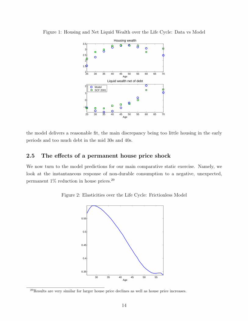
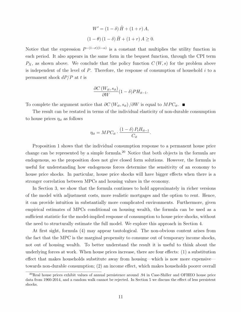
Figure 1: Housing and Net Liquid Wealth over the Life Cycle: Data vs Model

25 30 35 40 45 50 55 60 65 701

1.5

2

2.5

3

3.5Housing wealth

Age

25 30 35 40 45 50 55 60 65 70

−1

0

1

2

Liquid wealth net of debt

Age

ModelSCF 2001

the model delivers a reasonable fit, the main discrepancy being too little housing in the early

periods and too much debt in the mid 30s and 40s.

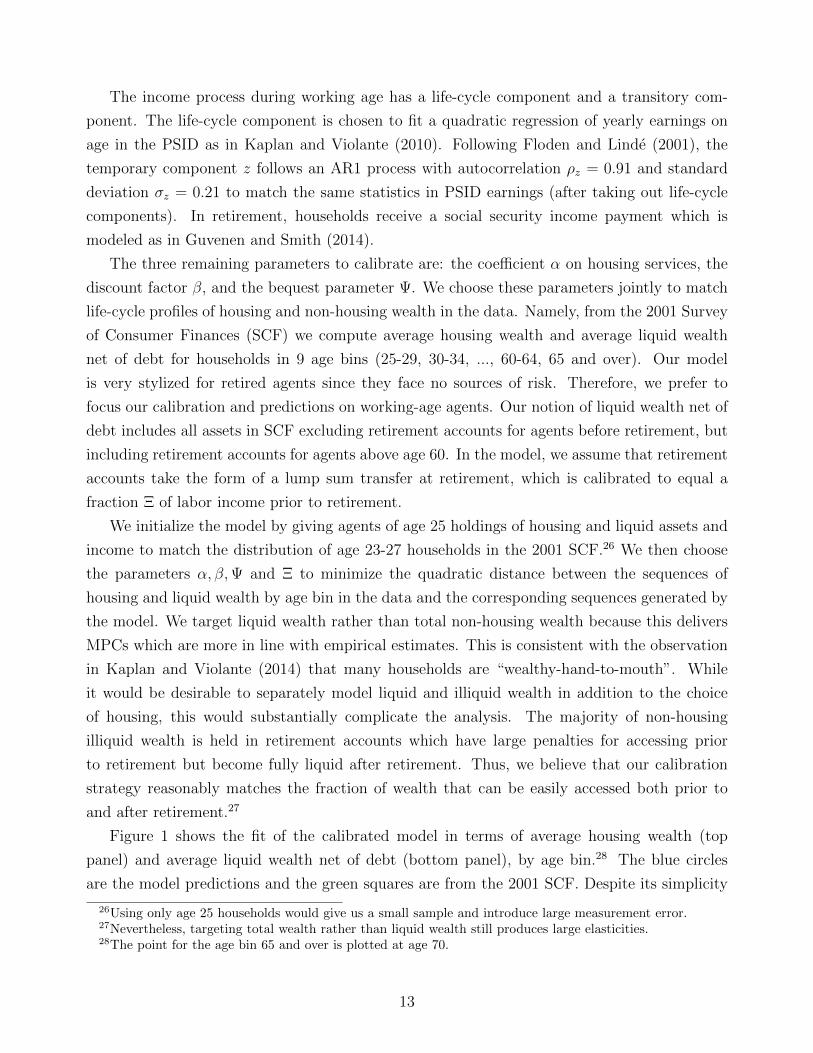
2.5 The effects of a permanent house price shock

We now turn to the model predictions for our main comparative static exercise. Namely, we

look at the instantaneous response of non-durable consumption to a negative, unexpected,

permanent 1% reduction in house prices.29

Figure 2: Elasticities over the Life Cycle: Frictionless Model

30 35 40 45 50 55

0.35

0.4

0.45

0.5

0.55

Age

29Results are very similar for larger house price declines as well as house price increases.

14

Figure 3: Understanding the Life Cycle: Frictionless Model

25 30 35 40 45 50 551

1.5

2

2.5

3

3.5Housing over the lifecycle

Age

25 30 35 40 45 50 550.05

0.1

0.15

0.2

0.25

0.3MPC over the lifecycle

Age

The average elasticity of consumption over working life is 0.47. Figure 2 reports elasticities

for different ages, with values as high as 0.6 for agents in their late 20s. Elasticities are higher

for younger agents and decline steadily after 30. The main takeaway is that magnitudes are

much larger than in the PIH model and are declining rather than increasing with age. In fact,

the elasticities obtained here are considerably larger than empirical estimates in the literature.

In the following section, we show that adding more realistic features to the model, and in

particular adding the option to rent, yields elasticities more in line with empirical estimates.

We can use our formula (4) to interpret this result. In Figure 3 we separately plot the two

elements of the formula: MPCs and housing values, averaged by age. The high elasticities of

young agents are driven by the fact that they have a high MPC and, at the same time, hold

substantial amounts of housing. In a precautionary saving model the MPC depends on total

net worth W and is decreasing in W due to concavity of the consumption function. Young

agents own houses but finance them with debt, so they have low net worth despite having

relatively high levels of housing. This explains the joint presence of high MPCs and high levels

of housing. Interestingly, our finding that young homeowners, who are more levered, exhibit

larger responses to house prices than old homeowners, who are less levered, is consistent with

the empirical finding in Attanasio et al. (2009).

2.6 Decomposing The House Price Effect

To conclude this section, we return to the decomposition of the consumption response intro-

duced in Subsection 2.3 and discuss its connection with the existing literature. As mentioned

before, the response can be decomposed into four effects: substitution, income, collateral, and

15

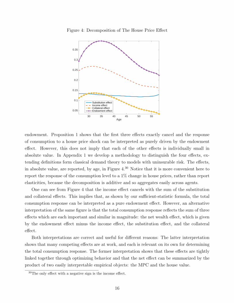
Figure 4: Decomposition of The House Price Effect

30 35 40 45 50 55Age

0.05

0.1

0.15

0.2

0.25

0.3

0.35

Substitution effectIncome effectCollateral effectEndowment effect

endowment. Proposition 1 shows that the first three effects exactly cancel and the response

of consumption to a house price shock can be interpreted as purely driven by the endowment

effect. However, this does not imply that each of the other effects is individually small in

absolute value. In Appendix 1 we develop a methodology to distinguish the four effects, ex-

tending definitions form classical demand theory to models with uninsurable risk. The effects,

in absolute value, are reported, by age, in Figure 4.30 Notice that it is more convenient here to

report the response of the consumption level to a 1% change in house prices, rather than report

elasticities, because the decomposition is additive and so aggregates easily across agents.

One can see from Figure 4 that the income effect cancels with the sum of the substitution

and collateral effects. This implies that, as shown by our sufficient-statistic formula, the total

consumption response can be interpreted as a pure endowment effect. However, an alternative

interpretation of the same figure is that the total consumption response reflects the sum of three

effects which are each important and similar in magnitude: the net wealth effect, which is given

by the endowment effect minus the income effect, the substitution effect, and the collateral

effect.

Both interpretations are correct and useful for different reasons: The latter interpretation

shows that many competing effects are at work, and each is relevant on its own for determining

the total consumption response. The former interpretation shows that these effects are tightly

linked together through optimizing behavior and that the net effect can be summarized by the

product of two easily interpretable empirical objects: the MPC and the house value.

30The only effect with a negative sign is the income effect.

16

To illustrate the usefulness of both interpretations, consider the large consumption response

in our model relative to the PIH model. Part of the large response in our model directly reflects

the addition of the collateral channel. In addition, unlike in the PIH model, the endowment

effect no longer approximately cancels with the income effect. Instead, the net wealth effect of

a house price increase is positive and sizable. The intuition for this result is that a permanent

increase in house prices leads to an immediate positive endowment effect while the increase in

rental costs occurs mostly in the future. Even though house price movements remain roughly

neutral for a household’s lifetime budget constraint, borrowing constraints mean that consump-

tion responds more to current than future income, so the endowment effect dominates. Thus,

the greater consumption response in our model relative to the PIH model can be interpreted

as an increase in the net wealth effect, with an additional collateral channel. Alternatively,

using our sufficient-statistic interpretation, it is immediate to see that the small consumption

response in the PIH model simply reflects the fact that this model implies a very small MPC.

The fact that borrowing constraints change the strength of the net wealth effect is also

important when using PIH intuition to empirically identify house price shocks on consumption.

For example, Attanasio et al. (2009) find that consumption of the young is more correlated

with house prices than that of the old and interpret this as evidence against housing wealth

shocks, since in a PIH framework, older households should respond more strongly to changes in

wealth due to their shorter planning horizon. Attanasio et al. (2011) validate this prediction in

a sophisticated quantitative model which relaxes the stylized PIH assumptions, but our results

show that this theoretical relationship does not hold in general and can be somewhat sensitive

to particular modeling choices. In our baseline results, the young respond much more strongly

to house price shocks. In the following section, we allow for rental markets and find that

consumption responses become largely independent of age. Our theoretical results show that

the age-profile of consumption responses will be determined by the age-profile of MPC × PH,

which our quantitative results show is theoretically ambiguous.31 Ultimately, this age-profile is

an empirical question, which we address in Section 4.

Our theoretical decomposition of housing price effects also helps reconcile our large elastic-

ities with the intuition of the “small house-price-effects” view mentioned in the introduction.

This view builds on the PIH model by arguing that, since changes in housing asset values are

offset by future changes in the user-cost of housing, ”housing wealth is not real wealth” and

should have little effect on consumption. For example, Sinai and Souleles (2005) argue that

this should be true when house price movements are perfectly correlated since everyone must

live somewhere. However, in their model there is no precautionary motive, which implies that

income and endowment effects exactly cancel; there are no substitution effects, as housing hold-

31This theoretical ambiguity might also help explain why some other studies such as Kaplan et al. (2015) andCampbell and Cocco (2007) find stronger effects for the old.

17

ings are fixed; and there are no collateral effects. Therefore, the three channels identified above

are absent.

Finally, our results have implications for the empirical literature measuring the strength of

the various channels through which house prices affect consumption. Each channel in our model

is large in isolation, so our model is quite consistent with the conclusions in DeFusco (2015) and

Mian et al. (2013) that there is a significant consumption response to housing collateral changes

and that the poorest and most indebted households respond most significantly to house price

movements through this channel. In particular, the collateral channel in our model implies

a marginal propensity to borrow of just over 10 cents, which is in line with the evidence in

DeFusco (2015). Nevertheless, it is important to note that the collateral effect in our model

is tightly linked to the other three effects, and that their sum eventually boils down to the

endowment effect alone, so the interpretation of the collateral effect in isolation must be done

with care.

3 Extended Model

In this section, we extend the model by relaxing various simplifying assumptions in order to get

a better quantitative assessment of housing price effects. In particular, we progressively enrich

the model by introducing adjustment costs to housing, the option to rent, and more realistic

mortgage contracts.

In terms of our sufficient-statistic approach, our main conclusion is that the formula derived

in Proposition 1 provides a good approximation for all realistic calibrations explored in this

section. This does not mean that the quantitative implications are insensitive to the different

specifications analyzed, since different specifications have different implications for the joint

distribution of housing wealth and MPCs. It just means that we can use the formula to

interpret the results obtained under all of our calibrations.

In terms of magnitudes, we still find fairly large elasticities under all the calibrations ex-

plored. The fully enriched model produces elasticities that are roughly half of what we found in

the baseline, and is thus closer to the empirical estimates. This is mostly due to the introduction

of the rental option, as we explain shortly.

3.1 Housing Transaction Costs

The assumption that housing can be traded frictionlessly is clearly counterfactual: search costs

and brokers’ fees make it costly to sell and buy houses, and indeed households trade houses only

18

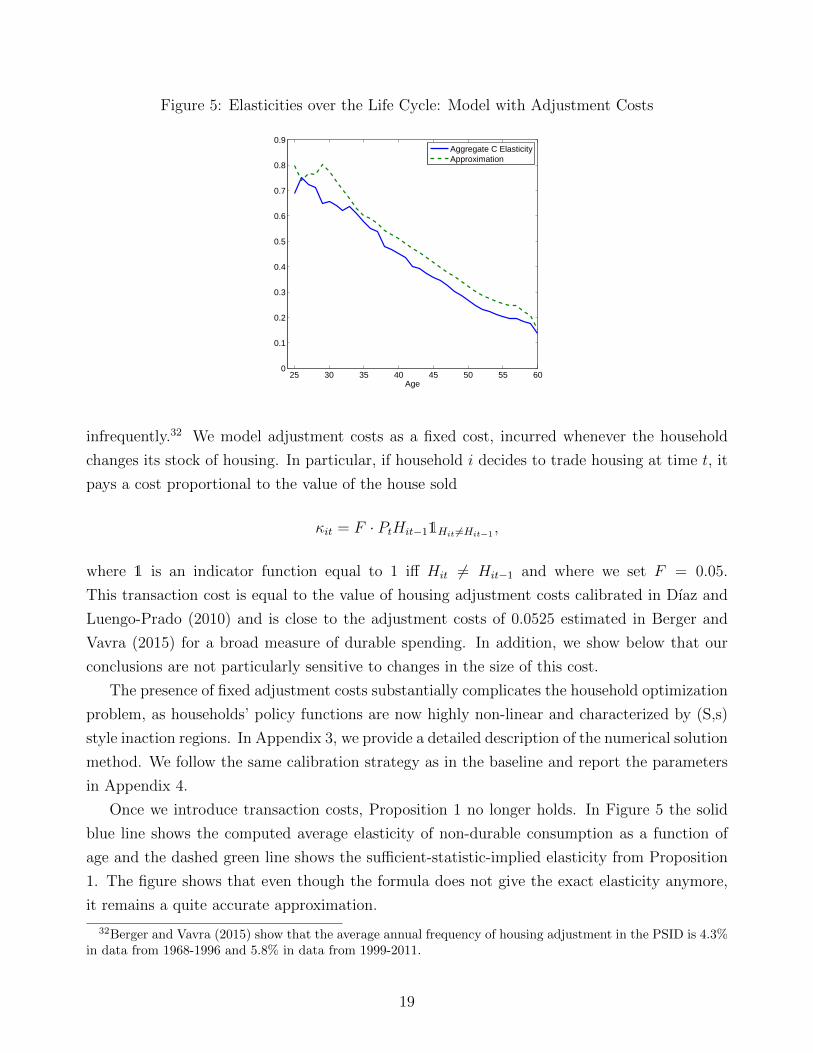
Figure 5: Elasticities over the Life Cycle: Model with Adjustment Costs

25 30 35 40 45 50 55 600

0.1

0.2

0.3

0.4

0.5

0.6

0.7

0.8

0.9

Age

Aggregate C ElasticityApproximation

infrequently.32 We model adjustment costs as a fixed cost, incurred whenever the household

changes its stock of housing. In particular, if household i decides to trade housing at time t, it

pays a cost proportional to the value of the house sold

κit = F · PtHit−11Hit 6=Hit−1,

where 1 is an indicator function equal to 1 iff Hit 6= Hit−1 and where we set F = 0.05.

This transaction cost is equal to the value of housing adjustment costs calibrated in Dıaz and

Luengo-Prado (2010) and is close to the adjustment costs of 0.0525 estimated in Berger and

Vavra (2015) for a broad measure of durable spending. In addition, we show below that our

conclusions are not particularly sensitive to changes in the size of this cost.

The presence of fixed adjustment costs substantially complicates the household optimization

problem, as households’ policy functions are now highly non-linear and characterized by (S,s)

style inaction regions. In Appendix 3, we provide a detailed description of the numerical solution

method. We follow the same calibration strategy as in the baseline and report the parameters

in Appendix 4.

Once we introduce transaction costs, Proposition 1 no longer holds. In Figure 5 the solid

blue line shows the computed average elasticity of non-durable consumption as a function of

age and the dashed green line shows the sufficient-statistic-implied elasticity from Proposition

1. The figure shows that even though the formula does not give the exact elasticity anymore,

it remains a quite accurate approximation.

32Berger and Vavra (2015) show that the average annual frequency of housing adjustment in the PSID is 4.3%in data from 1968-1996 and 5.8% in data from 1999-2011.

19

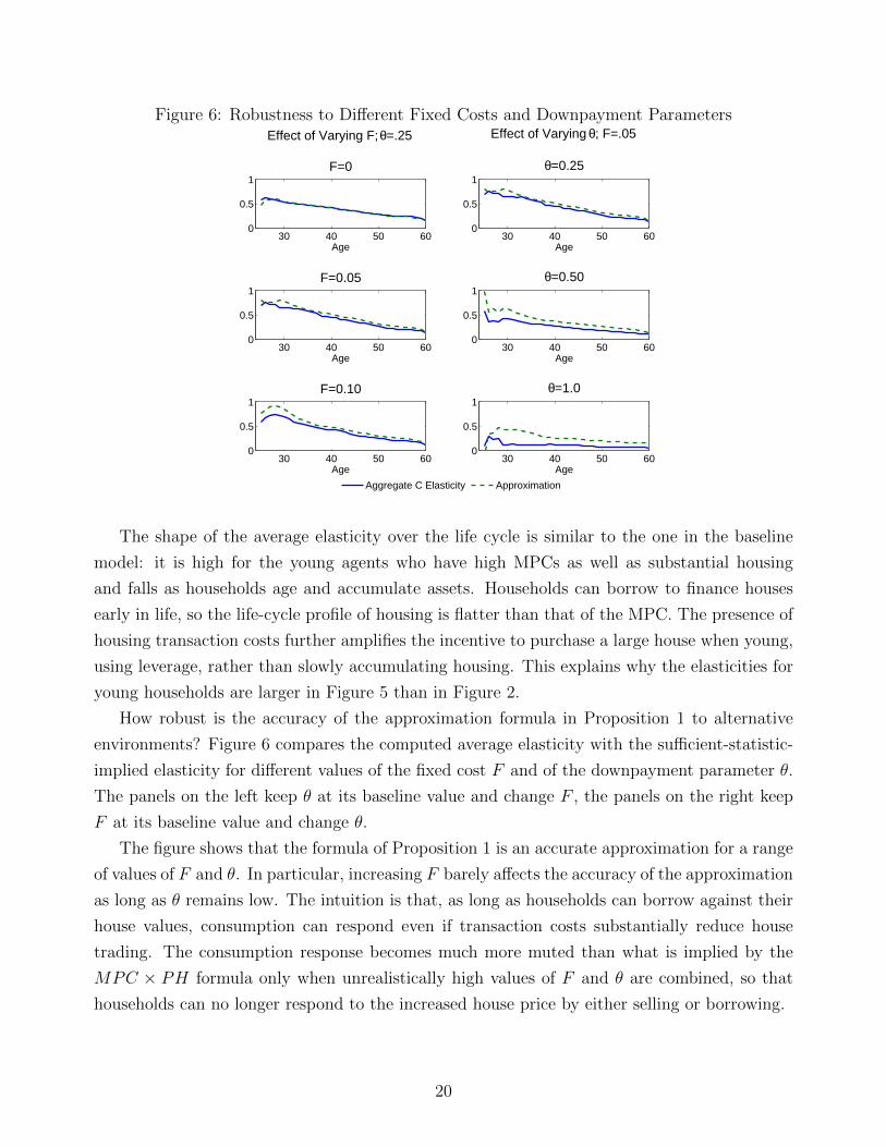
Figure 6: Robustness to Different Fixed Costs and Downpayment Parameters

30 40 50 600

0.5

1

Effect of Varying θ; F=.05

θ=0.25

Age

30 40 50 600

0.5

1θ=0.50

Age

30 40 50 600

0.5

1

Age

θ=1.0

Aggregate C Elasticity Approximation

30 40 50 600

0.5

1

Effect of Varying F; θ=.25

F=0

Age

30 40 50 600

0.5

1F=0.05

Age

30 40 50 600

0.5

1F=0.10

Age

The shape of the average elasticity over the life cycle is similar to the one in the baseline

model: it is high for the young agents who have high MPCs as well as substantial housing

and falls as households age and accumulate assets. Households can borrow to finance houses

early in life, so the life-cycle profile of housing is flatter than that of the MPC. The presence of

housing transaction costs further amplifies the incentive to purchase a large house when young,

using leverage, rather than slowly accumulating housing. This explains why the elasticities for

young households are larger in Figure 5 than in Figure 2.

How robust is the accuracy of the approximation formula in Proposition 1 to alternative

environments? Figure 6 compares the computed average elasticity with the sufficient-statistic-

implied elasticity for different values of the fixed cost F and of the downpayment parameter θ.

The panels on the left keep θ at its baseline value and change F , the panels on the right keep

F at its baseline value and change θ.

The figure shows that the formula of Proposition 1 is an accurate approximation for a range

of values of F and θ. In particular, increasing F barely affects the accuracy of the approximation

as long as θ remains low. The intuition is that, as long as households can borrow against their

house values, consumption can respond even if transaction costs substantially reduce house

trading. The consumption response becomes much more muted than what is implied by the

MPC × PH formula only when unrealistically high values of F and θ are combined, so that

households can no longer respond to the increased house price by either selling or borrowing.

20

3.2 Rental Markets

Roughly one third of US households rent rather than owning, and their wealth is not affected

by changes in house prices. Therefore, it is important to introduce a rental option. To do so,

we assume that in each period a household must choose whether to be a homeowner or a renter.

Renters pay a flow rental cost Rt per unit of housing services. Rental housing can be adjusted

costlessly but cannot be used as collateral. We assume that the rental cost Rt is proportional

to house prices, Rt = φPt, so that house price movements are passed proportionally into rental

costs.33

Households face a trade-off when choosing between renting and owning. The advantage

of renting is that it allows the household to keep its savings in the form of liquid assets,

thus providing a better buffer against income shocks. The disadvantage is that renting is

costlier, as we assume φ > (r + δ)/(1 + r),34 and rental housing cannot be used as collateral.35

Young households who are more financially constrained are the ones who benefit more from the

flexibility of renting and so will disproportionally choose to rent.

The rental-to-price ratio φ is an additional parameter of the model. We follow the previous

calibration strategy for all other parameters and choose φ to target the life-cycle profile of

homeownership rates. The parameters are reported in Appendix 4.36 Figure 7 shows that

we are still able to match the life-cycle profile of housing and liquid wealth reasonably well.

In addition, the model can fairly well match the upward slope and subsequent flattening of

homeownership rates over the life cycle.

How does the addition of the rental option affect the size of consumption responses to house

prices and the accuracy of our approximation? Figure 8 shows the actual average elasticity over

the life cycle for the model with and without the rental option (solid blue line and solid red

line). The figure also shows the sufficient-statistic approximation for both models (dashed blue

line and dashed red line). There are two takeaways from this figure. The first is that even with

the rental option, the sufficient-statistic formula of Proposition 1 remains a good approximation

of the true model elasticity. The second is that the addition of a rental option substantially

lowers the response of consumption to house prices, especially for the young households. The

average elasticity over working life goes from 0.43 in the model without the rental option to

33Using less than perfect passthrough amplifies elasticities.34Notice that (r + δ)/(1 + r)P is the user cost of housing services for a homeowner facing a constant house

price P .35The latter advantage is not enough, on its own, to induce households to own, because renting reduces the

need for borrowing more than it reduces the availability of collateral, since θ < 1.36At retirement, income risk falls to zero. This substantially changes the trade-off between liquid and illiquid

assets. With a constant rental rate this would imply a large jump up in the homeownership rate at retirement.To eliminate this jump, we introduce a different rental-to-price ratio at retirement φ < φ. This is isomorphicto a lower utility of housing in retirement, perhaps due to no longer having children at home or to greaterchallenges to home maintenance. At any rate, since we concentrate on results for working-age households, thechoice of φ has little effect on any of our results.

21

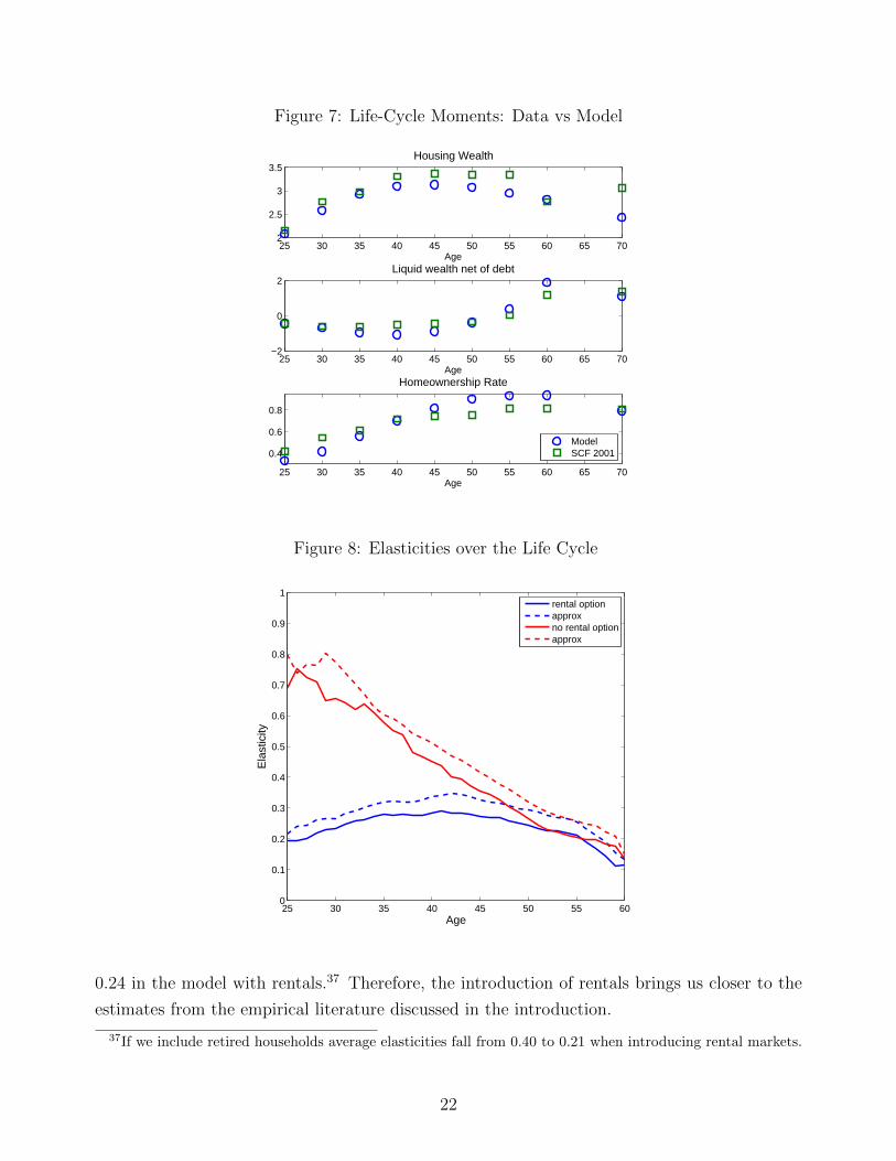
Figure 7: Life-Cycle Moments: Data vs Model

25 30 35 40 45 50 55 60 65 702

2.5

3

3.5Housing Wealth

Age

25 30 35 40 45 50 55 60 65 70−2

0

2Liquid wealth net of debt

Age

25 30 35 40 45 50 55 60 65 70

0.4

0.6

0.8

Homeownership Rate

Age

ModelSCF 2001

Figure 8: Elasticities over the Life Cycle

25 30 35 40 45 50 55 600

0.1

0.2

0.3

0.4

0.5

0.6

0.7

0.8

0.9

1

Age

Ela

stic

ity

rental optionapproxno rental optionapprox

0.24 in the model with rentals.37 Therefore, the introduction of rentals brings us closer to the

estimates from the empirical literature discussed in the introduction.

37If we include retired households average elasticities fall from 0.40 to 0.21 when introducing rental markets.

22

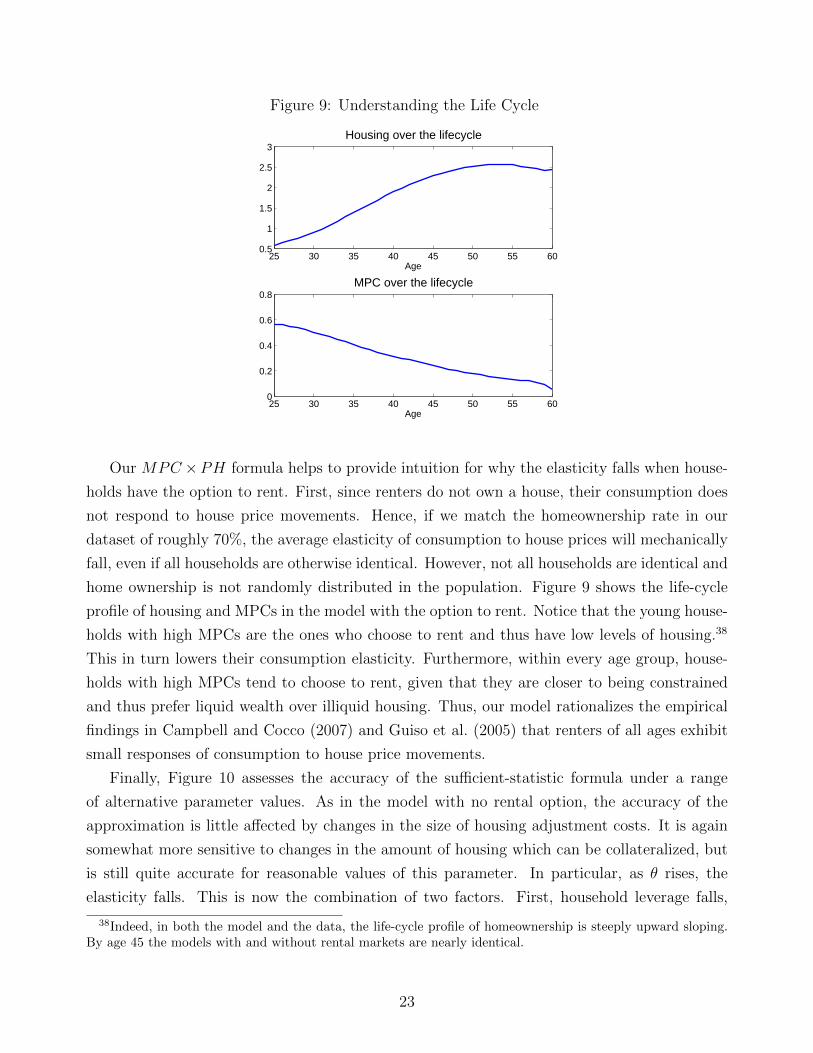
Figure 9: Understanding the Life Cycle

25 30 35 40 45 50 55 600.5

1

1.5

2

2.5

3Housing over the lifecycle

Age

25 30 35 40 45 50 55 600

0.2

0.4

0.6

0.8MPC over the lifecycle

Age

Our MPC ×PH formula helps to provide intuition for why the elasticity falls when house-

holds have the option to rent. First, since renters do not own a house, their consumption does

not respond to house price movements. Hence, if we match the homeownership rate in our

dataset of roughly 70%, the average elasticity of consumption to house prices will mechanically

fall, even if all households are otherwise identical. However, not all households are identical and

home ownership is not randomly distributed in the population. Figure 9 shows the life-cycle

profile of housing and MPCs in the model with the option to rent. Notice that the young house-

holds with high MPCs are the ones who choose to rent and thus have low levels of housing.38

This in turn lowers their consumption elasticity. Furthermore, within every age group, house-

holds with high MPCs tend to choose to rent, given that they are closer to being constrained

and thus prefer liquid wealth over illiquid housing. Thus, our model rationalizes the empirical

findings in Campbell and Cocco (2007) and Guiso et al. (2005) that renters of all ages exhibit

small responses of consumption to house price movements.

Finally, Figure 10 assesses the accuracy of the sufficient-statistic formula under a range

of alternative parameter values. As in the model with no rental option, the accuracy of the

approximation is little affected by changes in the size of housing adjustment costs. It is again

somewhat more sensitive to changes in the amount of housing which can be collateralized, but

is still quite accurate for reasonable values of this parameter. In particular, as θ rises, the

elasticity falls. This is now the combination of two factors. First, household leverage falls,

38Indeed, in both the model and the data, the life-cycle profile of homeownership is steeply upward sloping.By age 45 the models with and without rental markets are nearly identical.

23

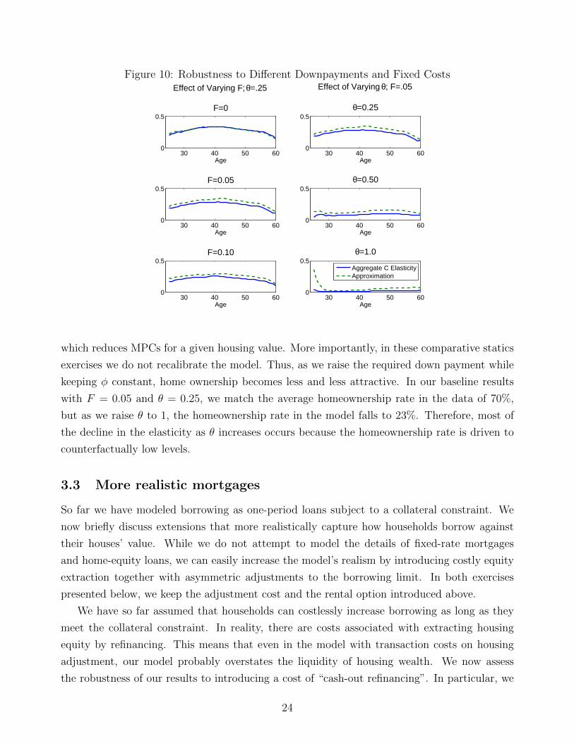
Figure 10: Robustness to Different Downpayments and Fixed Costs

30 40 50 600

0.5

Effect of Varying θ; F=.05

θ=0.25

Age

30 40 50 600

0.5θ=0.50

Age

30 40 50 600

0.5

Age

θ=1.0

Aggregate C ElasticityApproximation

30 40 50 600

0.5

Effect of Varying F; θ=.25

F=0

Age

30 40 50 600

0.5F=0.05

Age

30 40 50 600

0.5F=0.10

Age

which reduces MPCs for a given housing value. More importantly, in these comparative statics

exercises we do not recalibrate the model. Thus, as we raise the required down payment while

keeping φ constant, home ownership becomes less and less attractive. In our baseline results

with F = 0.05 and θ = 0.25, we match the average homeownership rate in the data of 70%,

but as we raise θ to 1, the homeownership rate in the model falls to 23%. Therefore, most of

the decline in the elasticity as θ increases occurs because the homeownership rate is driven to

counterfactually low levels.

3.3 More realistic mortgages

So far we have modeled borrowing as one-period loans subject to a collateral constraint. We

now briefly discuss extensions that more realistically capture how households borrow against

their houses’ value. While we do not attempt to model the details of fixed-rate mortgages

and home-equity loans, we can easily increase the model’s realism by introducing costly equity

extraction together with asymmetric adjustments to the borrowing limit. In both exercises

presented below, we keep the adjustment cost and the rental option introduced above.

We have so far assumed that households can costlessly increase borrowing as long as they

meet the collateral constraint. In reality, there are costs associated with extracting housing

equity by refinancing. This means that even in the model with transaction costs on housing

adjustment, our model probably overstates the liquidity of housing wealth. We now assess

the robustness of our results to introducing a cost of “cash-out refinancing”. In particular, we

24

extend the model by making the following assumption: if a household chooses positive holdings

of the risk-free asset At or if it chooses any At ≥ At−1 it can do so at no cost; but if the

household chooses a negative At smaller than At−1—i.e., if it increases its debt level—it must

pay a fixed cost.

Since the majority of refinancing costs do not depend on loan size, we model this cost as

a fixed numeraire amount, in contrast to the housing transaction cost which is proportional to

the size of the house.39 We pick this cost of refinancing to match the fraction of refinancing

observed in Bhutta and Keys (2014), which implies a fixed cost of 0.005.40 In the model with no

refinancing cost, roughly 30% of households increase debt each year while with the refinancing

cost, this number falls to a realistic 10%.41 Thus, refinancing costs substantially reduce the

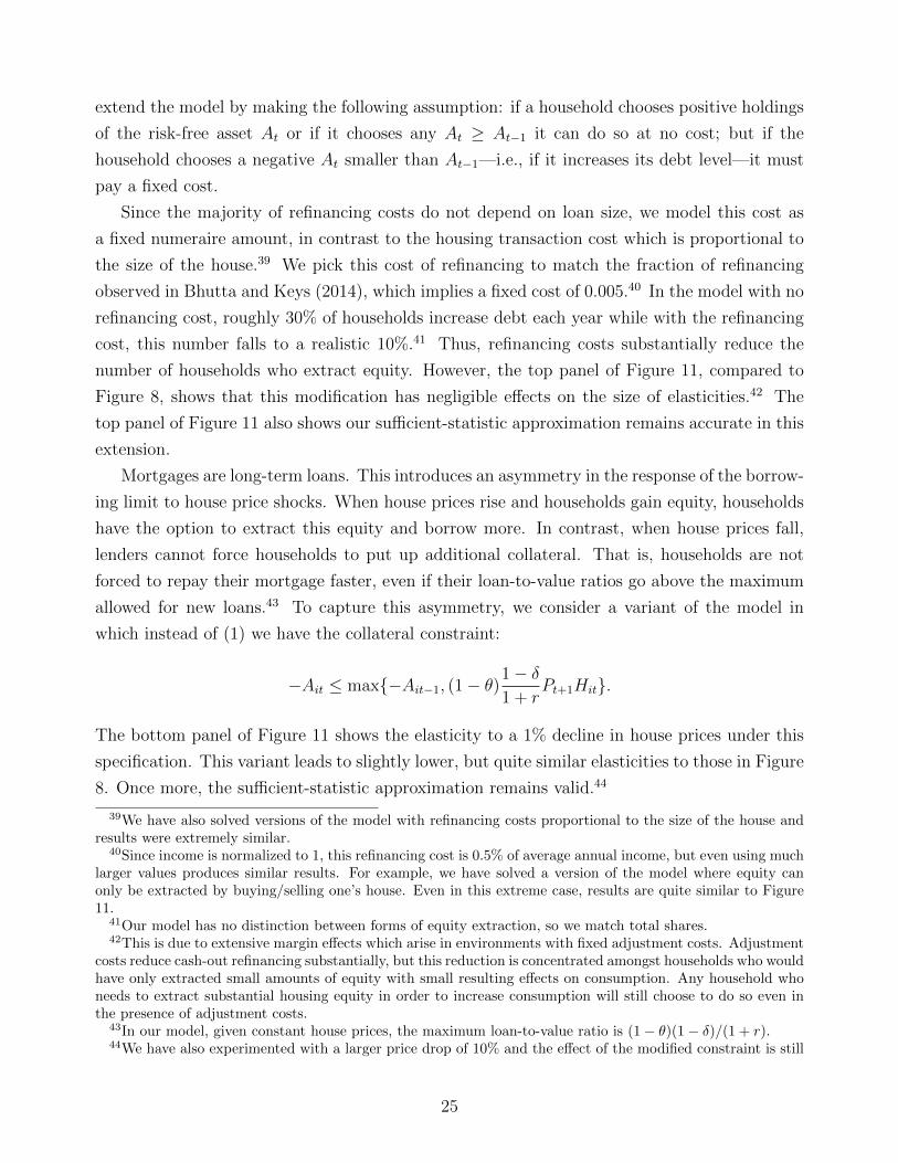
number of households who extract equity. However, the top panel of Figure 11, compared to

Figure 8, shows that this modification has negligible effects on the size of elasticities.42 The

top panel of Figure 11 also shows our sufficient-statistic approximation remains accurate in this

extension.

Mortgages are long-term loans. This introduces an asymmetry in the response of the borrow-

ing limit to house price shocks. When house prices rise and households gain equity, households

have the option to extract this equity and borrow more. In contrast, when house prices fall,

lenders cannot force households to put up additional collateral. That is, households are not

forced to repay their mortgage faster, even if their loan-to-value ratios go above the maximum

allowed for new loans.43 To capture this asymmetry, we consider a variant of the model in

which instead of (1) we have the collateral constraint:

−Ait ≤ max{−Ait−1, (1− θ)1− δ1 + r

Pt+1Hit}.

The bottom panel of Figure 11 shows the elasticity to a 1% decline in house prices under this

specification. This variant leads to slightly lower, but quite similar elasticities to those in Figure

8. Once more, the sufficient-statistic approximation remains valid.44

39We have also solved versions of the model with refinancing costs proportional to the size of the house andresults were extremely similar.

40Since income is normalized to 1, this refinancing cost is 0.5% of average annual income, but even using muchlarger values produces similar results. For example, we have solved a version of the model where equity canonly be extracted by buying/selling one’s house. Even in this extreme case, results are quite similar to Figure11.

41Our model has no distinction between forms of equity extraction, so we match total shares.42This is due to extensive margin effects which arise in environments with fixed adjustment costs. Adjustment

costs reduce cash-out refinancing substantially, but this reduction is concentrated amongst households who wouldhave only extracted small amounts of equity with small resulting effects on consumption. Any household whoneeds to extract substantial housing equity in order to increase consumption will still choose to do so even inthe presence of adjustment costs.

43In our model, given constant house prices, the maximum loan-to-value ratio is (1− θ)(1− δ)/(1 + r).44We have also experimented with a larger price drop of 10% and the effect of the modified constraint is still

25

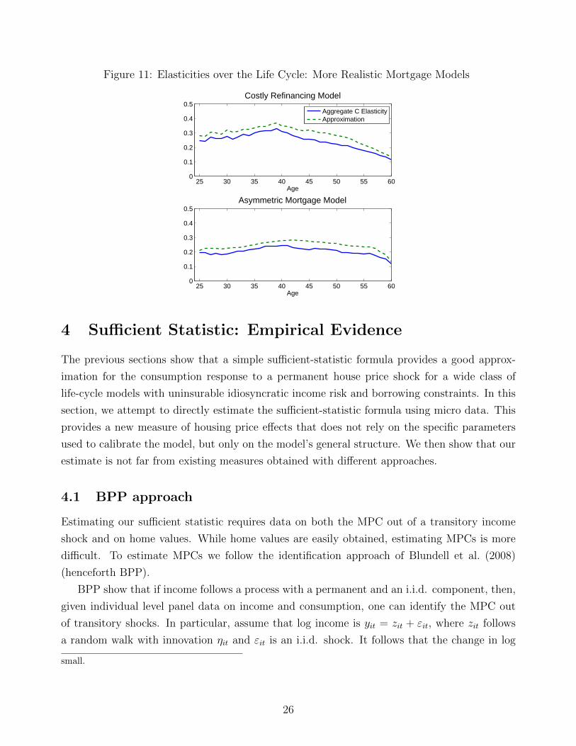
Figure 11: Elasticities over the Life Cycle: More Realistic Mortgage Models

25 30 35 40 45 50 55 600

0.1

0.2

0.3

0.4

0.5

Age

Costly Refinancing Model

Aggregate C ElasticityApproximation

25 30 35 40 45 50 55 600

0.1

0.2

0.3

0.4

0.5

Age

Asymmetric Mortgage Model

4 Sufficient Statistic: Empirical Evidence

The previous sections show that a simple sufficient-statistic formula provides a good approx-

imation for the consumption response to a permanent house price shock for a wide class of

life-cycle models with uninsurable idiosyncratic income risk and borrowing constraints. In this

section, we attempt to directly estimate the sufficient-statistic formula using micro data. This

provides a new measure of housing price effects that does not rely on the specific parameters

used to calibrate the model, but only on the model’s general structure. We then show that our

estimate is not far from existing measures obtained with different approaches.

4.1 BPP approach

Estimating our sufficient statistic requires data on both the MPC out of a transitory income

shock and on home values. While home values are easily obtained, estimating MPCs is more

difficult. To estimate MPCs we follow the identification approach of Blundell et al. (2008)

(henceforth BPP).

BPP show that if income follows a process with a permanent and an i.i.d. component, then,

given individual level panel data on income and consumption, one can identify the MPC out

of transitory shocks. In particular, assume that log income is yit = zit + εit, where zit follows

a random walk with innovation ηit and εit is an i.i.d. shock. It follows that the change in log

small.

26

income is equal to ∆yit = ηit + ∆εit.45 Given this income process, the true MPC (in logs) out

of a transitory shock is equal to

MPCt = cov(∆cit,εit)var(εit)

.

Under the assumption that households have no advanced information about future shocks, a

consistent estimator of this MPC is

MPCt = cov(∆cit,∆yit+t)cov(∆yit,∆yit+1)

.

With panel data containing at least three time periods, one can implement this estimator with

an instrumental variable regression of the change in consumption ∆cit on the change in income

∆yit, instrumenting for the current change in income with the future change in income, ∆yit+1.46

Since this requires individual level panel data on income and consumption, we use data from

the Panel Study of Income Dynamics (PSID).47

4.2 PSID data

Implementing our sufficient statistic empirically requires a longitudinal dataset with information

on income, consumption, and housing values at the household level. Starting from the 1999

wave, the PSID contains the necessary data. The PSID started collecting information on a

sample of roughly 5,000 households in 1968. Thereafter, both the original families and their

split-offs (children of the original family forming a family of their own) have been followed.

The survey was annual until 1996 and became biennial starting in 1997. In 1999 the survey

augmented the consumption information available to researchers so that it now covers over 70

percent of all consumption items available in the Consumer Expenditure Survey (CEX). This

is why we use 1999 as the first year of our sample.

Since we use almost the same underlying sample as Kaplan et al. (2014), our description of

the PSID closely mirrors theirs. We start with the PSID Core Sample and drop households with

missing information on race, education, or state of residence, and those whose income grows

more than 500 percent, falls by more than 80 percent, or is below $100. We drop households who

have top-coded income or consumption. We also drop households that appear in the sample

fewer than three consecutive times, because identification of the coefficients of interest requires

a minimum of three periods. In our baseline calculations, we keep households where the head

45Abowd and Card (1989) show that this parsimonious specification fits income data well.46We then convert this MPC in logs to the MPC in levels relevant for our theory by multiplying by C/Y .47An alternative approach to estimate MPCs, used by Johnson et al. (2006), uses random government rebate

timing and CEX data. Unfortunately, it is well known that the resulting standard errors on MPCS are largesince CEX data has much smaller sample sizes than PSID, no panel structure to disentangle true changes inconsumption from measurement error, and covers a smaller fraction of consumption. Large standard errors areespecially problematic for us, since we need to estimate MPCs conditional on different levels of housing wealth.

27

Figure 12: MPC and Housing

0.0

5.1

.15

.2M

PC

0 100000 200000 300000 400000 500000House Value

is 25-75 years old. Our final sample has 39,722 observations over the pooled years 1999-2011

(seven sample years).

We use the same consumption definition as Blundell et al. (2014), which covers approxi-

mately 70% of NIPA consumption. We define income as the sum of labor income and govern-

ment transfers. We purge the data of non-model features by regressing ln cit and ln yit on year

and cohort dummies, education, race, family structure, employment, geographic variables, and

interactions of year dummies with education, race, employment, and region.

4.3 Results

Since our formula is equal to the product of the MPC and the value of housing, we first examine

how the MPC varies with the value of housing. To do this, we estimate the MPC using the

BPP methodology separately in 6 housing bins. The first bin includes only renters—that is,

households who own zero housing. The other five bins are constructed as the quintiles of the

home value distribution and so are of equal size by construction. In total, in our database we

have approximately 15,000 renters and 25,000 home owners.

Figure 12 shows the relationship between the MPC and home values. Overall the rela-

tionship between home values and the MPC is flat or slightly declining (though this decline is

not statistically significant). Therefore, housing-rich households in the data still display high

MPCs, which will contribute to a large aggregate elasticity. Figure 13 translates these results

into elasticities by bins, which are computed by multiplying the MPC by bin in Figure 12 times

the ratio of average home values over average consumption in the same bin. Elasticities for

homeowners are non-monotone in housing and range between 0.11 and 0.63.

Using these estimates we can compute the aggregate elasticity of non-durable consumption

for the whole sample, which is equal to 0.33.48 This sufficient-statistic based measure of housing

48This value is given by (∑

kMPCk × PHk)/C, where MPCk is the estimated MPC in bin k, PHk is theaverage home value for bin k, and C is aggregate consumption.

28

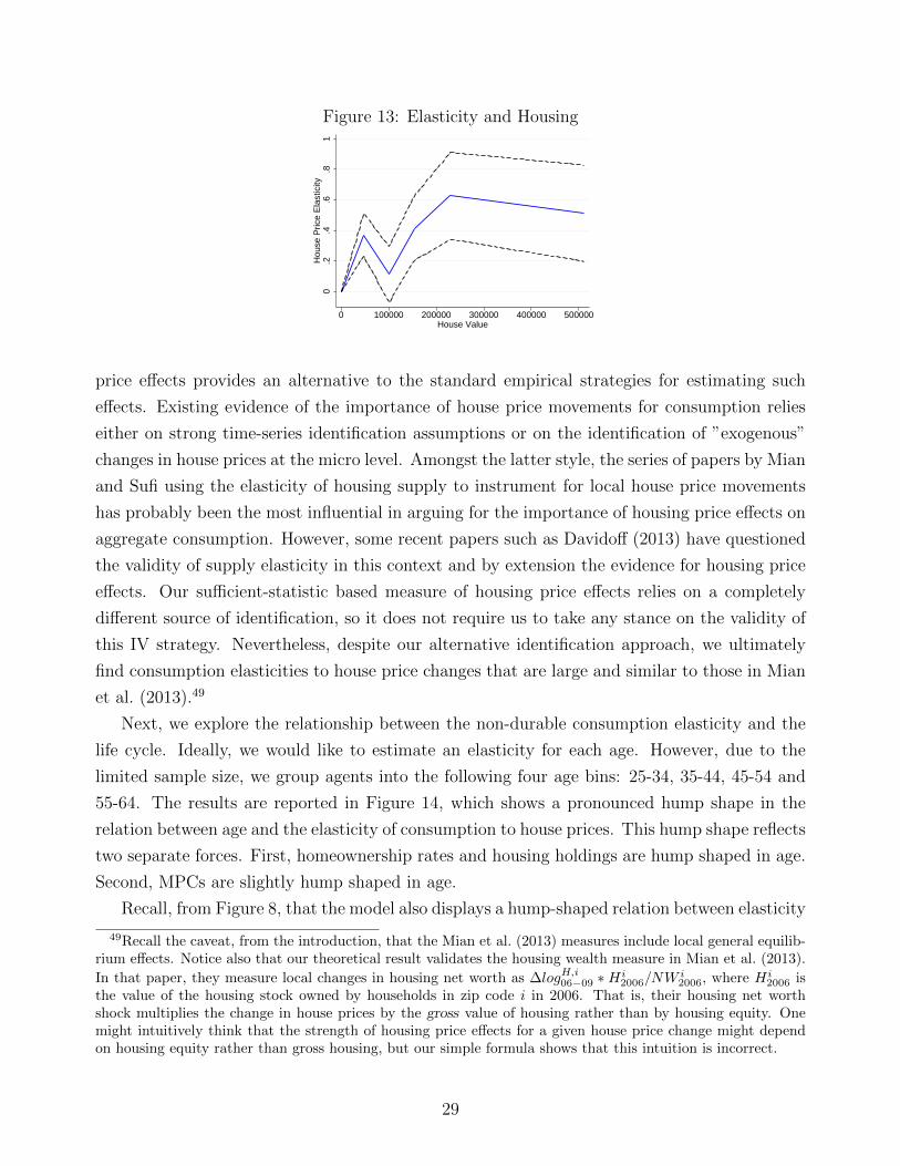
Figure 13: Elasticity and Housing

0.2

.4.6

.81

Hou

se P

rice

Ela

stic

ity0 100000 200000 300000 400000 500000

House Value

price effects provides an alternative to the standard empirical strategies for estimating such

effects. Existing evidence of the importance of house price movements for consumption relies

either on strong time-series identification assumptions or on the identification of ”exogenous”

changes in house prices at the micro level. Amongst the latter style, the series of papers by Mian

and Sufi using the elasticity of housing supply to instrument for local house price movements

has probably been the most influential in arguing for the importance of housing price effects on

aggregate consumption. However, some recent papers such as Davidoff (2013) have questioned

the validity of supply elasticity in this context and by extension the evidence for housing price

effects. Our sufficient-statistic based measure of housing price effects relies on a completely

different source of identification, so it does not require us to take any stance on the validity of

this IV strategy. Nevertheless, despite our alternative identification approach, we ultimately

find consumption elasticities to house price changes that are large and similar to those in Mian

et al. (2013).49

Next, we explore the relationship between the non-durable consumption elasticity and the

life cycle. Ideally, we would like to estimate an elasticity for each age. However, due to the

limited sample size, we group agents into the following four age bins: 25-34, 35-44, 45-54 and

55-64. The results are reported in Figure 14, which shows a pronounced hump shape in the

relation between age and the elasticity of consumption to house prices. This hump shape reflects

two separate forces. First, homeownership rates and housing holdings are hump shaped in age.

Second, MPCs are slightly hump shaped in age.

Recall, from Figure 8, that the model also displays a hump-shaped relation between elasticity

49Recall the caveat, from the introduction, that the Mian et al. (2013) measures include local general equilib-rium effects. Notice also that our theoretical result validates the housing wealth measure in Mian et al. (2013).

In that paper, they measure local changes in housing net worth as ∆logH,i06−09 ∗Hi

2006/NWi2006, where Hi

2006 isthe value of the housing stock owned by households in zip code i in 2006. That is, their housing net worthshock multiplies the change in house prices by the gross value of housing rather than by housing equity. Onemight intuitively think that the strength of housing price effects for a given house price change might dependon housing equity rather than gross housing, but our simple formula shows that this intuition is incorrect.

29

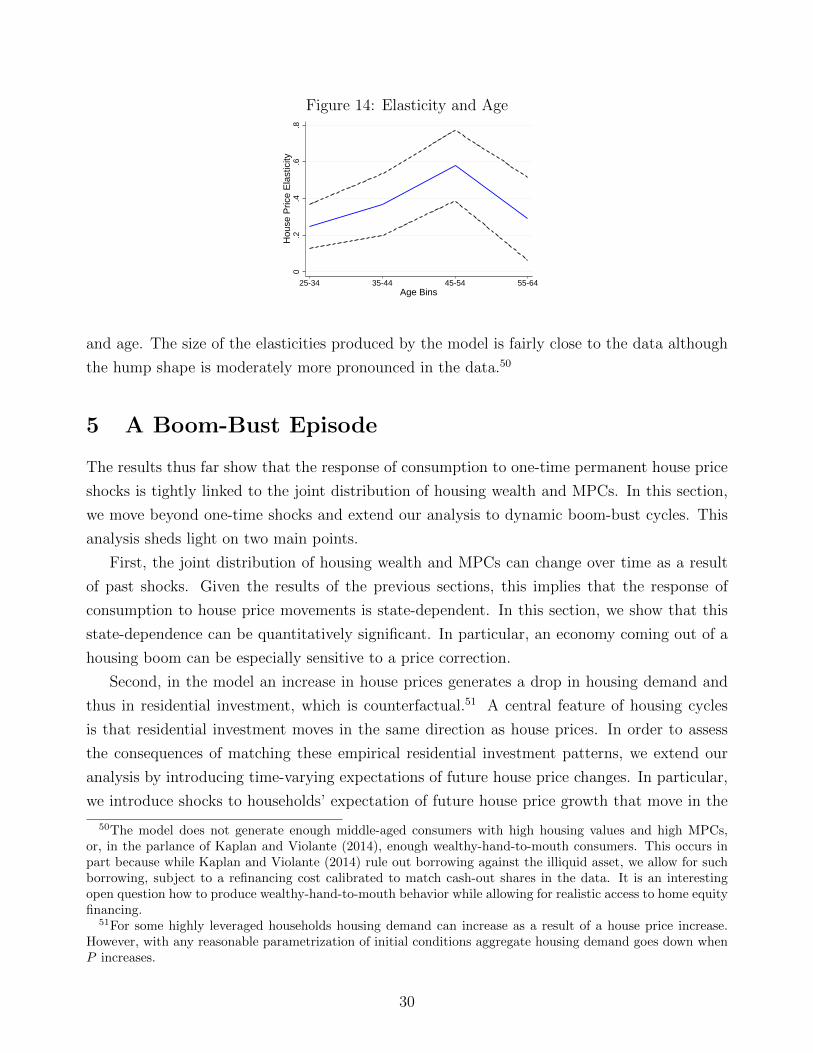
Figure 14: Elasticity and Age

0.2

.4.6

.8H

ouse

Pric

e E

last

icity

25-34 35-44 45-54 55-64Age Bins

and age. The size of the elasticities produced by the model is fairly close to the data although

the hump shape is moderately more pronounced in the data.50

5 A Boom-Bust Episode

The results thus far show that the response of consumption to one-time permanent house price

shocks is tightly linked to the joint distribution of housing wealth and MPCs. In this section,

we move beyond one-time shocks and extend our analysis to dynamic boom-bust cycles. This

analysis sheds light on two main points.

First, the joint distribution of housing wealth and MPCs can change over time as a result

of past shocks. Given the results of the previous sections, this implies that the response of

consumption to house price movements is state-dependent. In this section, we show that this

state-dependence can be quantitatively significant. In particular, an economy coming out of a

housing boom can be especially sensitive to a price correction.

Second, in the model an increase in house prices generates a drop in housing demand and

thus in residential investment, which is counterfactual.51 A central feature of housing cycles

is that residential investment moves in the same direction as house prices. In order to assess

the consequences of matching these empirical residential investment patterns, we extend our

analysis by introducing time-varying expectations of future house price changes. In particular,

we introduce shocks to households’ expectation of future house price growth that move in the

50The model does not generate enough middle-aged consumers with high housing values and high MPCs,or, in the parlance of Kaplan and Violante (2014), enough wealthy-hand-to-mouth consumers. This occurs inpart because while Kaplan and Violante (2014) rule out borrowing against the illiquid asset, we allow for suchborrowing, subject to a refinancing cost calibrated to match cash-out shares in the data. It is an interestingopen question how to produce wealthy-hand-to-mouth behavior while allowing for realistic access to home equityfinancing.

51For some highly leveraged households housing demand can increase as a result of a house price increase.However, with any reasonable parametrization of initial conditions aggregate housing demand goes down whenP increases.

30

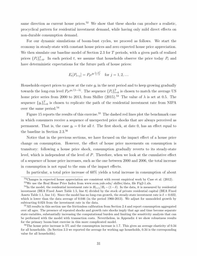
same direction as current house prices.52 We show that these shocks can produce a realistic,

procyclical pattern for residential investment demand, while having only mild direct effects on

non-durable consumption demand.

For our dynamic simulations of boom-bust cycles, we proceed as follows. We start the

economy in steady-state with constant house prices and zero expected house price appreciation.

We then simulate our baseline model of Section 2.3 for T periods, with a given path of realized

prices {Pt}Tt=0. In each period t, we assume that households observe the price today Pt and

have deterministic expectations for the future path of house prices:

Et[Pt+j] = Ptegt

1−λj1−λ for j = 1, 2, ....

Households expect prices to grow at the rate gt in the next period and to keep growing gradually

towards the long-run level Ptegt/(1−λ). The sequence {Pt}Tt=0 is chosen to match the average US

home price series from 2000 to 2013, from Shiller (2015).53 The value of λ is set at 0.5. The

sequence {gt}Tt=0 is chosen to replicate the path of the residential investment rate from NIPA

over the same period.54

Figure 15 reports the results of this exercise.55 The dashed red lines plot the benchmark case

in which consumers receive a sequence of unexpected price shocks that are always perceived as

permanent. That is, the case gt = 0 for all t. The first shock, at date 0, has an effect equal to

the baseline in Section 2.3.56

Notice that in the previous sections, we have focused on the impact effect of a house price

change on consumption. However, the effect of house price movements on consumption is

transitory: following a house price shock, consumption gradually reverts to its steady-state

level, which is independent of the level of P . Therefore, when we look at the cumulative effect

of a sequence of house price increases, such as the one between 2000 and 2006, the total increase

in consumption is not equal to the sum of the impact effects.

In particular, a total price increase of 60% yields a total increase in consumption of about

52Changes in expected house appreciation are consistent with recent empirical work by Case et al. (2012).53We use the Real Home Price Index from www.econ.yale.edu/ shiller/data, file Fig2-1.xls.54In the model, the residential investment rate is Ht+1/Ht− (1− δ). In the data, it is measured by residential

investment (BEA Fixed Asset Table 1.5, line 8) divided by the stock of private residential capital (BEA FixedAssets Table 1.1, line 14). Since the model has no long-run growth, the steady-state investment rate is δ = 0.022,which is lower than the data average of 0.046 (in the period 1960-2013). We adjust for unmodeled growth bysubtracting 0.024 from the investment rate in the data.

55All results in this section use the frictionless calibration from Section 2.4 and report consumption aggregatedover all ages. The presence of repeated shocks and growth rate shocks imply that age and time become separatestate-variables, substantially increasing the computational burden and limiting the sensitivity analysis that canbe performed with the model with transaction costs. Nevertheless, in Appendix 4 we show robustness resultsfor the primary boom-bust exercise in this more complicated model.

56The house price increase is 5% and the consumption increase is 1.7. This gives an average elasticity of 0.34for all households. (In Section 2.3 we reported the average for working age households, 0.34 is the correspondingvalue for all households).

31

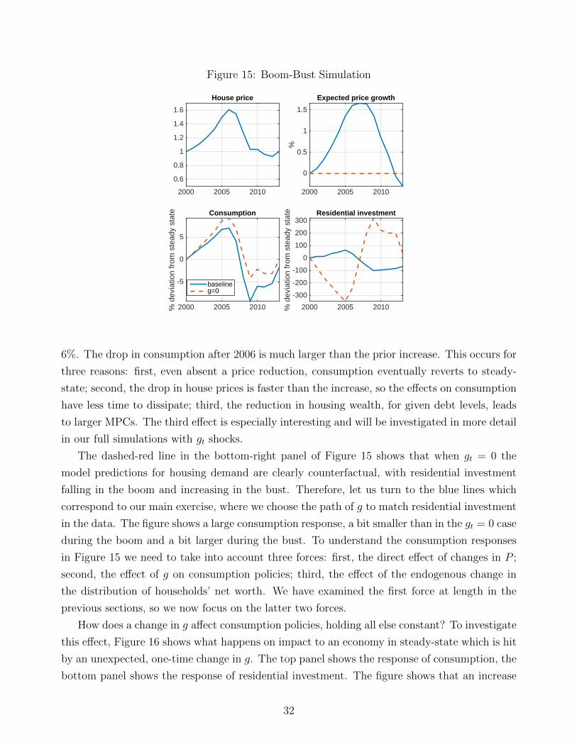
Figure 15: Boom-Bust Simulation

2000 2005 2010

0.6

0.8

1

1.2

1.4

1.6

House price

2000 2005 2010

%

0

0.5

1

1.5

Expected price growth

2000 2005 2010% d

evia

tion

from

ste

ady

stat

e

-5

0

5

Consumption

baselineg=0

2000 2005 2010% d

evia

tion

from

ste

ady

stat

e-300

-200

-100

0

100

200

300Residential investment

6%. The drop in consumption after 2006 is much larger than the prior increase. This occurs for

three reasons: first, even absent a price reduction, consumption eventually reverts to steady-

state; second, the drop in house prices is faster than the increase, so the effects on consumption

have less time to dissipate; third, the reduction in housing wealth, for given debt levels, leads

to larger MPCs. The third effect is especially interesting and will be investigated in more detail

in our full simulations with gt shocks.

The dashed-red line in the bottom-right panel of Figure 15 shows that when gt = 0 the

model predictions for housing demand are clearly counterfactual, with residential investment

falling in the boom and increasing in the bust. Therefore, let us turn to the blue lines which

correspond to our main exercise, where we choose the path of g to match residential investment

in the data. The figure shows a large consumption response, a bit smaller than in the gt = 0 case

during the boom and a bit larger during the bust. To understand the consumption responses

in Figure 15 we need to take into account three forces: first, the direct effect of changes in P ;

second, the effect of g on consumption policies; third, the effect of the endogenous change in

the distribution of households’ net worth. We have examined the first force at length in the

previous sections, so we now focus on the latter two forces.

How does a change in g affect consumption policies, holding all else constant? To investigate

this effect, Figure 16 shows what happens on impact to an economy in steady-state which is hit

by an unexpected, one-time change in g. The top panel shows the response of consumption, the

bottom panel shows the response of residential investment. The figure shows that an increase

32

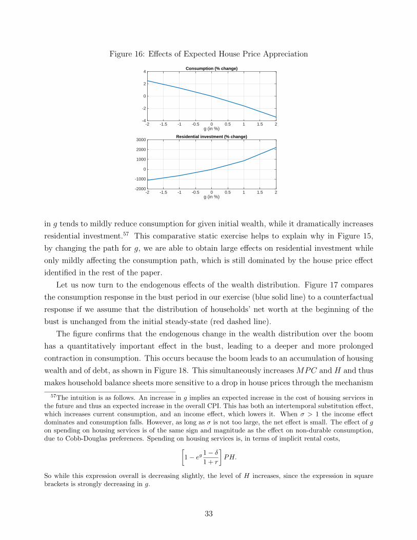
Figure 16: Effects of Expected House Price Appreciation

g (in %)-2 -1.5 -1 -0.5 0 0.5 1 1.5 2

-4

-2

0

2

4Consumption (% change)

g (in %)-2 -1.5 -1 -0.5 0 0.5 1 1.5 2

-2000

-1000

0

1000

2000

3000Residential investment (% change)

in g tends to mildly reduce consumption for given initial wealth, while it dramatically increases

residential investment.57 This comparative static exercise helps to explain why in Figure 15,

by changing the path for g, we are able to obtain large effects on residential investment while

only mildly affecting the consumption path, which is still dominated by the house price effect

identified in the rest of the paper.

Let us now turn to the endogenous effects of the wealth distribution. Figure 17 compares

the consumption response in the bust period in our exercise (blue solid line) to a counterfactual

response if we assume that the distribution of households’ net worth at the beginning of the

bust is unchanged from the initial steady-state (red dashed line).

The figure confirms that the endogenous change in the wealth distribution over the boom

has a quantitatively important effect in the bust, leading to a deeper and more prolonged

contraction in consumption. This occurs because the boom leads to an accumulation of housing

wealth and of debt, as shown in Figure 18. This simultaneously increases MPC and H and thus

makes household balance sheets more sensitive to a drop in house prices through the mechanism

57The intuition is as follows. An increase in g implies an expected increase in the cost of housing services inthe future and thus an expected increase in the overall CPI. This has both an intertemporal substitution effect,which increases current consumption, and an income effect, which lowers it. When σ > 1 the income effectdominates and consumption falls. However, as long as σ is not too large, the net effect is small. The effect of gon spending on housing services is of the same sign and magnitude as the effect on non-durable consumption,due to Cobb-Douglas preferences. Spending on housing services is, in terms of implicit rental costs,[

1− eg 1− δ1 + r

]PH.

So while this expression overall is decreasing slightly, the level of H increases, since the expression in squarebrackets is strongly decreasing in g.

33

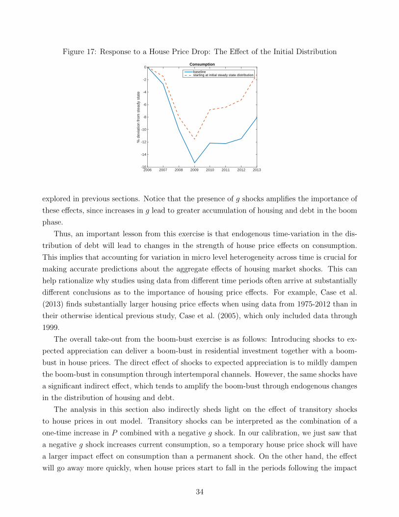
Figure 17: Response to a House Price Drop: The Effect of the Initial Distribution

2006 2007 2008 2009 2010 2011 2012 2013

% d

evia

tion

from

ste

ady

stat

e

-16

-14

-12

-10

-8

-6

-4

-2

0Consumption

baselinestarting at initial steady state distribution

explored in previous sections. Notice that the presence of g shocks amplifies the importance of

these effects, since increases in g lead to greater accumulation of housing and debt in the boom

phase.

Thus, an important lesson from this exercise is that endogenous time-variation in the dis-

tribution of debt will lead to changes in the strength of house price effects on consumption.

This implies that accounting for variation in micro level heterogeneity across time is crucial for

making accurate predictions about the aggregate effects of housing market shocks. This can

help rationalize why studies using data from different time periods often arrive at substantially

different conclusions as to the importance of housing price effects. For example, Case et al.

(2013) finds substantially larger housing price effects when using data from 1975-2012 than in

their otherwise identical previous study, Case et al. (2005), which only included data through

1999.

The overall take-out from the boom-bust exercise is as follows: Introducing shocks to ex-

pected appreciation can deliver a boom-bust in residential investment together with a boom-

bust in house prices. The direct effect of shocks to expected appreciation is to mildly dampen

the boom-bust in consumption through intertemporal channels. However, the same shocks have

a significant indirect effect, which tends to amplify the boom-bust through endogenous changes

in the distribution of housing and debt.

The analysis in this section also indirectly sheds light on the effect of transitory shocks

to house prices in out model. Transitory shocks can be interpreted as the combination of a

one-time increase in P combined with a negative g shock. In our calibration, we just saw that

a negative g shock increases current consumption, so a temporary house price shock will have

a larger impact effect on consumption than a permanent shock. On the other hand, the effect

will go away more quickly, when house prices start to fall in the periods following the impact

34

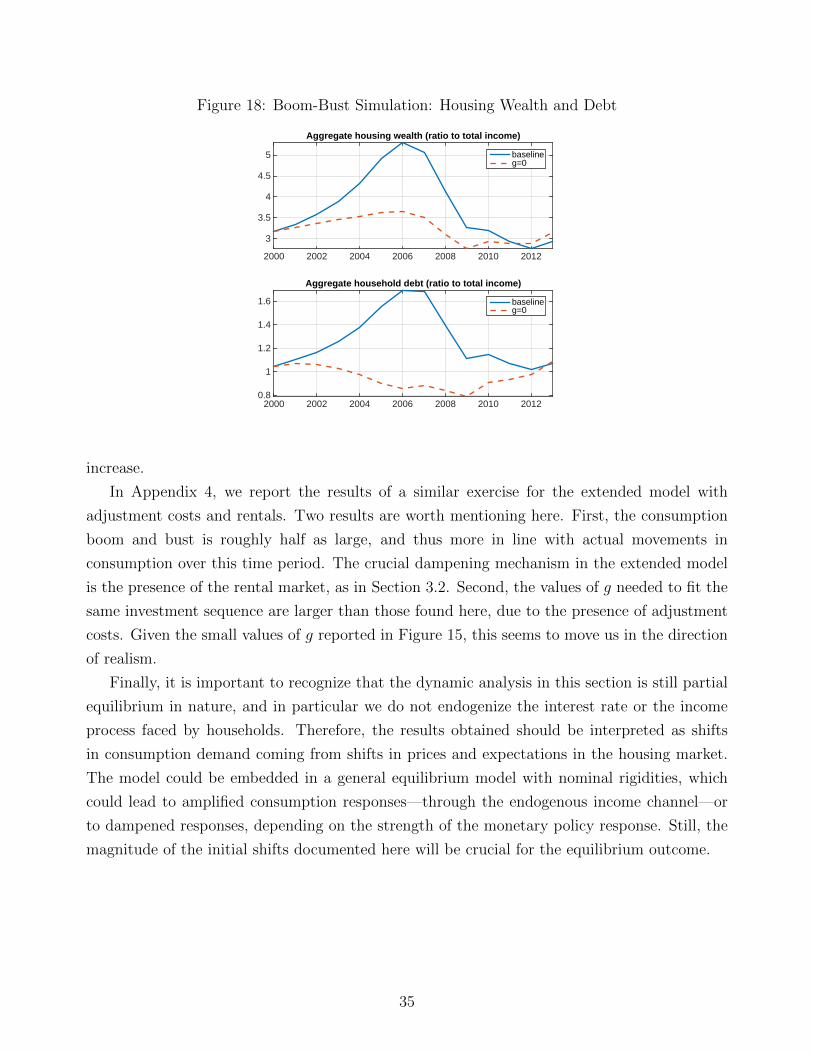
Figure 18: Boom-Bust Simulation: Housing Wealth and Debt

2000 2002 2004 2006 2008 2010 2012

3

3.5

4

4.5

5

Aggregate housing wealth (ratio to total income)

baselineg=0

2000 2002 2004 2006 2008 2010 20120.8

1

1.2

1.4

1.6

Aggregate household debt (ratio to total income)

baselineg=0

increase.

In Appendix 4, we report the results of a similar exercise for the extended model with

adjustment costs and rentals. Two results are worth mentioning here. First, the consumption

boom and bust is roughly half as large, and thus more in line with actual movements in

consumption over this time period. The crucial dampening mechanism in the extended model

is the presence of the rental market, as in Section 3.2. Second, the values of g needed to fit the

same investment sequence are larger than those found here, due to the presence of adjustment

costs. Given the small values of g reported in Figure 15, this seems to move us in the direction

of realism.

Finally, it is important to recognize that the dynamic analysis in this section is still partial

equilibrium in nature, and in particular we do not endogenize the interest rate or the income

process faced by households. Therefore, the results obtained should be interpreted as shifts

in consumption demand coming from shifts in prices and expectations in the housing market.

The model could be embedded in a general equilibrium model with nominal rigidities, which

could lead to amplified consumption responses—through the endogenous income channel—or

to dampened responses, depending on the strength of the monetary policy response. Still, the

magnitude of the initial shifts documented here will be crucial for the equilibrium outcome.

35

6 Conclusion

In this paper, we explore the implications of consumption theory for understanding housing

price effects on consumption. While a large and growing empirical literature documents strong

responses of consumption to identified house price movements, a large theoretical literature

argues that this response should be small.

We show that a relatively standard incomplete markets consumption model with idiosyn-

cratic risk actually implies quite large elasticities, and we derive a new sufficient statistic to

provide intuition for this large value. This sufficient statistic continues to work well in more

realistic models, and we show that these models deliver elasticities closely in line with empirical

evidence. We then take our sufficient statistic directly to micro data and show it yields similar

conclusions. Not only is our sufficient statistic useful for understanding why elasticities in our

model are large, it also provides good intuition for why some previous models have found small

elasticities. These models often either imply counterfactually small MPCs or shut down some

of the theoretical channels through which house prices can affect consumption.

Our results also imply that the size of housing price effects may vary substantially across

households and time. Indeed, we find large variation over the boom-bust in our model and

find that elasticities vary substantially with age and home ownership status. The presence of

this time-variation and heterogeneity may help reconcile various empirical results and should

be accounted for when predicting the aggregate consequences of housing market policies.

36

References

Abowd, John M. and David Card, “On the Covariance Structure of Earnings and Hours

Changes,” Econometrica, 1989, 57 (2), 411–445.

Aguiar, Mark and Erik Hurst, “Deconstructing Lifecycle Expenditures,” Journal of Polit-

ical Economy, 2013, 212 (1).

Attanasio, Orazio and Guglielmo Weber, “The UK consumption boom of the late 1980s:

aggregate implications of microeconomic evidence,” The Economic Journal, 1994, pp. 1269–

1302.

, Andrew Leicester, and Matthew Wakefield, “Do House Prices Drive Consumption

Growth? The Coincident Cycles of House Prices and Consumption in the UK,” Journal of

the European Economic Association, 2011, 9 (3).

, Laura Blow, Robert Hamilton, and Andrew Leicester, “Booms and Busts: Con-

sumption, House Prices, and Expectations,” Economica, 2009, 76 (301), 20–50.

Auclert, Adrien, “Monetary Policy and the Redistribution Channel,” 2015. mimeo, Stanford

University.

Berger, David and Joseph Vavra, “Consumption Dynamics During Recessions,” Econo-

metrica, 2015, 83 (1), 101—154.

Bhutta, Neil and Benjamin J. Keys, “Interest Rates and Equity Extraction During the

Housing Boom,” University of Chicago Kreisman Working Papers Series in Housing Law

and Policy, 2014, 3.

Blundell, Richard, Luigi Pistaferri, and Ian Preston, “Consumption Inequality and

Partial Insurance,” American Economic Review, 2008, 98 (5), 1887—1921.

, , and Itay Saporta-Eksten, “Consumption Inequality and Family Labor Supply,” 2014

Meeting Papers No. 322 Society for Economic Dynamics, 2014.

Buiter, Willem H., “Housing Wealth Isn’t Wealth,” NBER Working Paper 14204, 2008.

Caballero, Ricardo and Eduardo M. R. A. Engel, “Explaining Investment Dynamics in

U.S. Manufacturing: A Generalized (S,s) Approach,” Econometrica, 1999, 67 (4), 783—826.

Campbell, John Y. and Joao F. Cocco, “How Do House Prices Affect Consumption?,”

Journal of Monetary Economics, 2007, 54 (3), 591—621.

37

and , “A Model of Mortgage Default,” Journal of Finance (Forthcoming), 2015.

Carroll, Chris and Wendy Dunn, “Unemployment Expectations, Jumping (S,s) Triggers,

and Household Balance Sheets,” NBER Maroeconomics Annual, 1998, 12, 165—230.

Carroll, Christopher D., Misuzu Otsuka, and Jiri Slacalek, “How Large Are Housing

and Financial Wealth Effects? A New Approach,” Journal of Money Credit and Banking,

2011, 1 (43), 55—79.

Case, Karl E., John M. Quigley, and Robert J. Shiller, “Comparing Wealth Effects:

The Stock Market versus the Housing Market,” Advances in Macroeconomics, 2005, 5 (1).

, , and , “Wealth Effects Revisited: 1975-2012,” Critical Finance Review, 2013, 2 (1),

101—128.

, Robert J. Shiller, and Anne Thompson, “What Have They Been Thinking? Home

Buyer Behavior in Hot and Cold Markets,” NBER Working Paper 18400, 2012.

Cerutti, Eugenio, Jihad Dagher, and Mr Giovanni Dell’Ariccia, “Housing Finance and

Real-Estate Booms: A Cross-Country Perspective,” Staff Discussion Notes 15/12, Interna-

tional Monetary Fund 2015.

Chetty, Raj, “Sufficient Statistics for Welfare Analysis: A Bridge Between Structural and

Reduced-Form Methods,” Annual Review of Economics, 2009, 1, 451—488.

Corbae, Dean and Erwan Quintin, “Leverage and the Foreclosure Crisis,” Journal of

Political Economy, 2015, 123 (1), 1—65.

Davidoff, Thomas, “Supply Elasticity and the Housing Cycle of the 2000s,” Real Estate

Economics, 2013, 41 (4), 793—813.

Davis, Morris A. and Francois Ortalo-Magne, “Household Expenditures, Wages, Rents,”

Review of Economic Dynamics, 2011, 14, 248—261.

DeFusco, Anthony, “Homeowner Borrowing and Housing Collateral: New Evidence from

Expiring Price Controls,” 2015.

Dıaz, Antonia and Marıa Jose Luengo-Prado, “The Wealth Distribution with Durable

Goods,” International Economic Review, 2010, 51 (1), 143—170.

Eggertsson, Gauti B and Paul Krugman, “Debt, deleveraging, and the liquidity trap: A

fisher-minsky-koo approach*,” The Quarterly Journal of Economics, 2012.

38

Favilukis, Jack, Sydney C. Ludvigson, and Stijn Van Nieuwerburgh, “The Macroe-

conomic Effects of Housing Wealth, Housing Finance, and Limited Risk-Sharing in General

Equilibrium,” Working Paper, NYU 2015.

Floden, Martin and Jesper Linde, “Idiosyncratic Risk in the United States and Sweden:

Is There a Role for Government Insurance,” Review of Economic Dynamics, 2001, 4 (2),

406—437.

Gorea, Denis and Virgiliu Midrigan, “Liquidity Constraints in the U.S. Housing Market,”

2015.

Guerrieri, Veronica and Guido Lorenzoni, “Credit Crises, Precautionary Savings, and

the Liquidity Trap,” Working Paper, National Bureau of Economic Research 2011.

Guiso, Luigi, Monica Paiella, and Ignazio Visco, “Do capital gains affect consumption?

Estimates of wealth effects from italian households’ behavior,” Temi di discussione 555, Bank

of Italy 2005.

Guvenen, Fatih and Anthony A. Smith, “Inferring Labor Income Risk and Partial Insur-

ance from Economic Choices,” Econometrica, 2014, 82 (6), 2085—2129.

Hall, Robert E, “The Long Slump,” American Economic Review, 2011, 101 (2), 431–69.

He, Chao, Randall Wright, and Yu Zhu, “Housing and liquidity,” Review of Economic

Dynamics, 2014.

Huo, Zhen and Jose-Vıctor Rıos-Rull, “Balance sheet recessions,” Technical Report,

Working Paper, Federal Reserve Bank of Minneapolis 2013.

Johnson, David S., Jonathan A. Parker, and Nicholas S. Souleles, “Household Ex-

penditure and the Income Tax Rebates of 2001,” American Economic Review, 2006, 96 (5),

1589—1610.

Justiniano, Alejandro, Giorgio E Primiceri, and Andrea Tambalotti, “Credit Supply

and the Housing Boom,” mimeo, Northwestern 2015.

, , and , “Household leveraging and deleveraging,” Review of Economic Dynamics, 2015,

18 (1), 3–20.

Kaplan, Greg and Gianluca Violante, “How Much Consumption Insurance Beyond Self-

Insurance,” American Economic Journals: Macroeconomics, 2010, 2 (4), 53—87.

39

and , “A Model of the Consumption Response to Fiscal Stimulus Payments,” Economet-

rica, 2014, 82 (4), 1199—1239.

, Giovanni L. Violante, and Justin Weidner, “The Wealthy Hand-To-Mouth,” NBER

Working Paper 20073, 2014.

, Kurt Mitman, and Gianluca Violante, “Consumption and House Prices in The Great

Recession,” 2015.

Mian, Atif, Kamalesh Rao, and Amir Sufi, “Household Balance Sheets, Consumption,

and the Economic Slump,” The Quarterly Journal of Economics, 2013, 128 (4), 1687—1726.

Midrigan, Virgiliu and Thomas Philippon, “Household Leverage and the Recession,”

Technical Report 16965, NBER 2011.

Petev, Ivaylo, Luigi Pistaferri, and Itay Saporta Eksten, “Consumption and the Great

Recession: An analysis of trends, perceptions, and distributional effects,” in D. Grusky,

B. Western, and C. Wimer, eds., Analyses of the Great Recession, 2012.

Piazzesi, Monika, Martin Schneider, and Selale Tuzel, “Housing, Consumption and

Asset Pricing,” Journal of Financial Economics, 2007, 83, 531—569.

Saiz, Albert, “The Geographic Determinants of Housing Supply,” The Quarterly Journal of

Economics, 2010, 125 (3), 1253—1296.

Shiller, Robert J., “Irrational Exuberance,” Princeton University Press, 2015.

Sinai, Todd and Nicholas S Souleles, “Owner-Occupied Housing as a Hedge against Rent

Risk,” The Quarterly Journal of Economics, 2005, pp. 763–789.

Stroebel, Johannes and Joseph Vavra, “House Prices, Local Demand, and Retail Prices,”

2015.

Tauchen, George, “Finite State Markov-Chain Approximations to Univariate and Vector

Autoregressions,” Economics Letters, 1986, 20 (2), 177—181.

Vavra, Joseph, “Inflation Dynamics and Time-Varying Volatility: New Evidence and an Ss

Interpretation,” The Quarterly Journal of Economics, 2014, 129 (1), 215—258.

Winberry, Thomas, “Lumpy Investment, Business Cycles, and Stimulus Policy,” 2015.

40

Online Appendix (Not For Publication)

House Prices and Consumer Spending

D. Berger, V. Guerrieri, G. Lorenzoni, J. Vavra

1 Decomposition

In this section we derive decompositions of the total house price effect into income, substitution,

collateral and endowment effects and discuss their interpretation both for the simple PIH model

of Subection 2.2 and for the general baseline model treated in the rest of Section 2.

1.1 PIH model

For simplicity, we focus on the infinite-horizon version of the model and drop the individual

subscript i. The household’s utility function is∑∞

t=0 βtU (Ct, Ht). The per-period budget con-

straints, with a no Ponzi condition, can be aggregated into the intertemporal budget constraint

at date 0:

∞∑t=0

qt [Ct + [Pt − q (1− δ)Pt+1]Ht − Yt] = (1 + r)A−1 + (1− δ)P0H−1,

where q ≡ 1/ (1 + r). Define the implicit rental rate

Rt ≡ Pt − q (1− δ)Pt+1.

Suppose that the house price is initially constant at P so that the implicit rental rate is then

R = (1− q (1− δ))P . We then want to decompose the response of C0 to a permanent change

in P .

Define the Marshallian demand for C0

C0 = C0,m (R, I) ,

which comes from maximizing∑βtU (Ct, Ht) subject to

∑qt [Ct +RHt] = I. Similarly, define

the Hicksian demand

C0 = C0,h (R,U) ,

which comes from minimizing∑qt [Ct +RHt] subject to

∑βtU (Ct, Ht) ≥ U . The effect of a

permanent change dR is equivalent to summing the effects of identical changes in the price of

housing services dRt. So the standard decomposition result also applies and implies that the

1

total response of consumption to a change in P satisfies

dC0

dP= [1− q (1− δ)] ∂C0,h (R,U)

∂R−[1− q (1− δ)] ∂C0,m (R, I)

∂I

∑qtHt+

∂C0,m (R, I)

∂I(1− δ)H−1.

The first term is the substitution effect, the second the income effect, the third the endowment

effect.

Under the assumption of Cobb-Douglas preferences and q = β, the solution to the household

problem gives a constant level of housing Ht = H0 and of consumption Ct = C0 with

C0 = αr

1 + r

[(1 + r)A−1 + (1− δ)P0H−1 +

∑qtYt

].

Now consider a household that starts at H−1 = H0 (which applies for small changes in R, for

a household that started life at any time t < 0). Then the sum of the income and endowment

effects is

∂C0,m (R, I)

∂I

{− [1− q (1− δ)]

∑qt + (1− δ)

}H = − δ

1− q∂C0,m (R, I)

∂IH < 0.

The net effect is small if δ is small, and exactly zero if δ = 0. This capture the Sinai and

Souleles (2005) intuition that when the price of houses increases, and the net present value of

implicit rental cost increases by the same amount, then there are small wealth effects. That

the net effect is actually negative reflects the fact that the consumer is a net buyer of housing

since he needs to replace the depreciated fraction of housing in all periods.

At the same time, we know that

dC0

dP= α

r

1 + r(1− δ)H−1 =

∂C0,m (R, I)

∂I(1− δ)H−1 > 0.

This implies that the total effect can be interpreted in two ways:

• a substitution effect that more than compensates for the negative net of income and

endowment effects derived above;

• a pure endowment effect, with the substitution and income effects canceling each other.

1.2 General model with no adjustment costs

Given the household’s optimization problem on page 10, with Pt = P for all t, let C(W, s;P, θ)

denote the optimal consumption policy. Consider the effects of an unexpected, permanent

change in price from P0 to P1. Let (H−, A−) denote the household initial holdings of housing

2

and of the risk-free asset. Household net wealth is then

W0 = P0 (1− δ)H− + (1 + r)A−

before the shock, and

W1 = P1 (1− δ)H− + (1 + r)A−

after the shock. The total consumption change is

∆C ≡ C(W1, s;P1, θ)− C(W0, s;P0, θ).

To compute the collateral effect choose θ such that

(1− θ)P1 =(

1− θ)P0,

that is consider a change in the collateral requirement that exactly offsets the change in price.

The collateral effect is then defined as

CE ≡ C(W0, s;P0, θ

)− C (W0, s;P0, θ) .

Next, find the value of initial wealth W such that V(W , s;P1, θ

)= V

(W0, s;P0, θ

). That

is, we find the wealth that keeps utility unchanged after a change in the price of housing.

Here, we are adapting the logic of Hicksian compensation to our dynamic, incomplete-markets

problem. We define the substitution effect as

SE ≡ C(W , s;P1, θ

)− C

(W0, s;P0, θ

),

where the change in θ is introduced to mute the collateral effect and the change in W is

introduced to mute the income effect. The income effect is given by

IE ≡ C (W0, s;P1, θ)− C(W , s;P1, θ

).

Finally, the endowment effect is just given by

EE ≡ C (W1, s;P1, θ)− C (W0, s;P1, θ) ,

and elementary algebra gives

∆C = SE + IE + CE + EE,

3

and since C(W, s;P, θ) is independent of P , as shown in Proposition 1, we have ∆C = EE.

Notice that the exact result of the decomposition, for discrete changes in P , depends on the

ordering (e.g., here we started from the collateral effect).

2 Extension: CES Preferences

In this section, we extend the analysis to CES preferences for consumption and housing. In

the body of the paper, we assume Cobb-Douglas utility—i.e., elasticity of substitution equal to

1—and use that assumption to derive Proposition 1. Here we show that the proposition can be

extended to the case of CES preferences if we make the additional assumption of θ = 0, that is,

if we consider a very loose collateral requirement. In that case, our sufficient statistic formula

extends naturally by adding a new term that is positive in the case of elasticity of substitution

bigger than 1 and negative in the opposite case. We then provide numerical results for the case

θ > 0, calibrated as in the main text, and show that, for reasonable values of the elasticity

of substitution between consumption and housing, our amended sufficient-statistic formula

provides a good approximation and the additional term has small effects if the elasticity of

subsitution is in the range 0.8− 1.25. Overall, under plausible parametrizations the magnitude

of the elasticity remains large.

Let the utility function be:

U (Cit, Hit) =1

1− σ

(αC

ε−1ε

it + (1− α)Hε−1ε

it

) ε(1−σ)ε−1

where ε is the intra-temporal elasticity of substitution between non-durable consumption and

housing services.

Proposition 2 Consider the model with CES preferences, liquid housing wealth, and θ = 0.

The individual response of non-durable consumption to an unexpected, permanent, proportional

change in house prices dP/P is

(ε− 1)r+δ1+r

PHit

Cit + r+δ1+r

PHit

Cit +MPCit · (1− δ)PHit−1.

Proof. With constant prices, the user cost of housing (or implicit rental rate) is r+δ1+r

P . So we

can define total spending on non-durables and housing services

Xit ≡ Cit +r + δ

1 + rPHit,

4

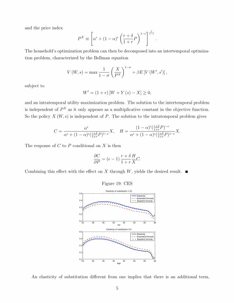
and the price index

PX ≡

[αε + (1− α)ε

(r + δ

1 + rP

)1−ε] 1

1−ε

.

The household’s optimization problem can then be decomposed into an intertemporal optimiza-

tion problem, characterized by the Bellman equation

V (W, s) = max1

1− σ

(X

PX

)1−σ

+ βE [V (W ′, s′)] ,

subject to

W ′ = (1 + r) [W + Y (s)−X] ≥ 0,

and an intratemporal utility maximization problem. The solution to the intertemporal problem

is independent of PX as it only appears as a multiplicative constant in the objective function.

So the policy X (W, s) is independent of P . The solution to the intratemporal problem gives

C =αε

αε + (1− α)ε( r+δ1+r

P )1−εX, H =

(1− α)ε( r+δ1+r

P )−ε

αε + (1− α)ε( r+δ1+r

P )1−εX.

The response of C to P conditional on X is then

∂C

∂P= (ε− 1)

r + δ

1 + r

H

XC.

Combining this effect with the effect on X through W , yields the desired result.

Figure 19: CES

25 30 35 40 45 50 55 600.1

0.2

0.3

0.4

0.5

Age

Elasticity of substitution 1.25

ElasticityExtended formulaBaseline formula

25 30 35 40 45 50 55 600.1

0.2

0.3

0.4

0.5Elasticity of substitution 0.8

Age

ElasticityExtended formulaBaseline formula

An elasticity of substitution different from one implies that there is an additional term,

5

proportional to the implicit share of housing services in the total consumption basket. In the

model, this share is tightly linked to the ratio of house values to consumption. For example,

take an agent with housing-to-consumption ratio 3.5—which is the roughly the average for

agents in the 40s bin. With r = 2.4% and δ = 2.2% this implies a share of housing services

to total spending equal to 0.13. For such an agent if ε = 1.1, the additional term is equal to

0.1×0.13 = 0.013. If the same agent has an MPC of 0.1 the magnitude of the baseline sufficient

statistic is 0.1× 3.5 = 0.35, so the additional term plays a minor role quantitatively.

For the case θ > 0 analytical results are not available and we turn to simulations. Namely,

for different values of ε we re-calibrate the model to hit the same targets as in the baseline

and compute the elasticity of consumption to house prices. In Figure 19 we plot the computed

elasticity for different age bins, together with our baseline formula and our amended formula.

We present results for the two cases ε = 0.8 and ε = 1.2. The amended formula provides a good

approximation and the baseline still gives magnitudes close to the true responses.

3 Description of Computational Procedures

In this appendix, we describe the solution to the model with transaction costs and rental

described in the body of the text. The household state vector is s ≡ (A,H, z, j), and the model

is solved by backward induction from the final period of life. When working, households solve:

V (s) = max{V adjust(s), V noadjust(s), V rent(s)

}.

The three value functions, for adjusters, non-adjusters, and renters, are given by

V adjust(s) = maxC,A′,H′

U (C,H ′) + βE [V (s′)|z]

s.t. A′ + PH ′ + C = (1 + r)A+ Y (z) + (1− F ) (1− δ)PH,

A′ ≥ − (1− θ) 1− δ1 + r

PH ′, s′ = (A′, H ′, z′, j + 1),

V noadjust(s) = maxC,A′

U (C,H) + βE [V (s′)|z]

s.t. A′ + C = (1 + r)A+ Y (z)− δPH,

A′ ≥ − (1− θ) 1− δ1 + r

PH, s′ = (A′, H, z′, j + 1),

6

V rent(s) = maxC,A′,H

U(C, H

)+ βE [V (s′)|z]

s.t. A′ + C + φPH = (1 + r)A+ Y (z) + (1− F ) (1− δ)PH,

A′ ≥ 0, s′ = (A′, 0, z′, j + 1).

The problem for a retired household is identical except that social security benefits replace labor

earnings. At the age of retirement households also receive an additional lump sump transfer to

match the level of retirement wealth which is now liquid, as described in the text. At the time

of death households’ continuation value is given by the bequest motive in the text.

To solve the model numerically, we proceed as follows. First, in order to rectangularize

the choice set and simplify the computational problems imposed by the endogenous liquidity

constraint, we follow Dıaz and Luengo-Prado (2010) and reformulate our problem in terms of

voluntary equity, defined as

Q ≡ A+ (1− θ) 1− δ1 + r

PH.

After substituting the budget constraint into the utility function to eliminate C as a choice

variable, the value function can then be rewritten in terms of the two non-negative state vari-

ables Q′ and H ′. Note that A′ and H ′ are chosen prior to next period shocks to house prices.

Thus, shocks to house prices imply that realized voluntary equity will differ from the value

chosen in the previous period. Namely, given a chosen pair Q′, H ′, the realized value of Q next

period will be Q′ + (1− θ) 1−δ1+r

H ′∆P , where ∆P is the house price shock. This implies that

although households are constrained to always choose Q′ ≥ 0, realized voluntary equity can

be negative, for a large enough negative house price shock. To account for this, we solve the

model for states that include negative voluntary equity even though households are constrained

to choose non-negative values for this variable.58

We discretize the problem so it can be solved on the computer by first discretizing z using

the algorithm of Tauchen (1986). We use 13 grid points for z. We then approximate the

functions V adjustj , V noadjust

j , and V rentj as mulitlinear functions in the endogenous states. In

our benchmark calculation, we use 120 knot points for Q (we space these points more closely

together near the constraint) and 40 knot points for H. The presence of fixed adjustment costs

on housing together with the borrowing constraint make the household policy function highly

non-linear. For this reason, we follow Berger and Vavra (2015) and compute optimal policies for

a given state-vector using a Nelder-Meade algorithm initialized from 3 different starting values,

to reduce the problem of finding local maxima. The value of adjusting, not adjusting and

renting are then compared to generate the overall policy function. We proceed via backward

induction from the final period of life.

58Shocks to house prices in the model are not large enough to ever reach a situation where realized Q is sonegative that households would be unable to choose Q′ ≥ 0 without having negative consumption.

7

Figure 20: Housing and Net Liquid Wealth over the Life Cycle: Data vs Model

25 30 35 40 45 50 55 60 65 700.5

1

1.5

2

2.5

3Housing Wealth

Age

25 30 35 40 45 50 55 60 65 70−2

−1

0

1

2Liquid wealth net of debt

Age

ModelSCF 2001

To simulate the model, we initialize cohorts to match the values of the SCF for age 22-27

year old households. First, we randomly split the sample into two groups to match the fraction

of homeowners and renters. Then within each group, we split the sample into 4 income bins

and assign the median value of housing and liquid assets from the SCF in that same income

bin. (By definition, the value of housing for the renter groups is always zero). The model is

simulated with 100,000 households and house price impulse responses are computed for each

cohort.

In the boom-bust episode, house price expectations become an additional state-variable,

and the model is solved and simulated for the combination of each age-calendar time pair.

4 Additional Quantitative Results and Calibration De-

tails

This section shows a number of numerical results and details which are suppressed from the

main text for brevity.

Table 2 shows the best fit parameters for the model with transaction costs but no rental

market, and Figure 20 shows the corresponding model fit.

Table 2: Parameter Values for Model with Fixed Costs and No Rent

Parameter σ r δ θ ρz σz α β Ψ ΞValue 2 2.4% 2.2% 0.25 0.91 0.21 0.875 0.922 2, 300 1.75

Table 3 shows the best fit parameters for the model with transaction costs and rental

8

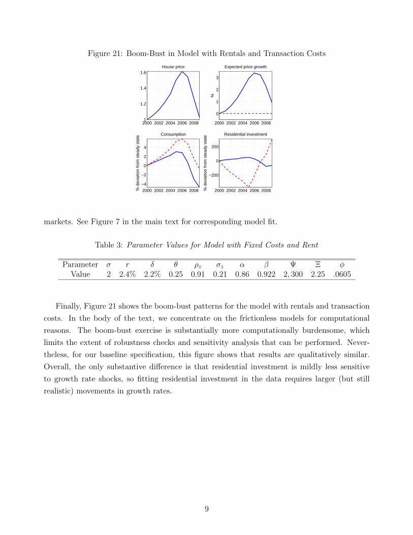
Figure 21: Boom-Bust in Model with Rentals and Transaction Costs

2000 2002 2004 2006 20081

1.2

1.4

1.6House price

2000 2002 2004 2006 2008

0

1

2

3

Expected price growth

%

2000 2002 2004 2006 2008

−4

−2

0

2

4

% d

evia

tion

from

ste

ady

stat

e Consumption

2000 2002 2004 2006 2008

−200

0

200

% d

evia

tion

from

ste

ady

stat

e Residential investment

markets. See Figure 7 in the main text for corresponding model fit.

Table 3: Parameter Values for Model with Fixed Costs and Rent

Parameter σ r δ θ ρz σz α β Ψ Ξ φValue 2 2.4% 2.2% 0.25 0.91 0.21 0.86 0.922 2, 300 2.25 .0605

Finally, Figure 21 shows the boom-bust patterns for the model with rentals and transaction

costs. In the body of the text, we concentrate on the frictionless models for computational

reasons. The boom-bust exercise is substantially more computationally burdensome, which

limits the extent of robustness checks and sensitivity analysis that can be performed. Never-

theless, for our baseline specification, this figure shows that results are qualitatively similar.

Overall, the only substantive difference is that residential investment is mildly less sensitive

to growth rate shocks, so fitting residential investment in the data requires larger (but still

realistic) movements in growth rates.

9