Hours and Employment Implications of Search Frictions: Matching

Aggregate and Establishment-level Observations ∗

Russell Cooper†, John Haltiwanger‡, and Jonathan L. Willis§

September 4, 2006

Abstract

This paper studies worker and job flows at the establishment and aggregate levels. The paper is

built around a set of facts concerning the variability of unemployment and vacancies in the aggregate,

the distribution of net employment growth and the comovement of hours and employment growth at

the establishment level. A search model with frictions in hiring and firing is used as a framework to

understand these observations. Notable features of this search model include non-convex costs of posting

vacancies, establishment level shocks and a contracting framework that determines the response of hours

and wages to shocks. We specify and estimate the parameters of the search model using simulated

method of moments to match establishment-level and aggregate observations.

1 Motivation

This paper studies the implications of a search model estimated from both microeconomic and macroeconomic

data. This paper is motivated partly as an attempt to match labor market facts and partly as an exercise to

bring together two disparate perspectives on frictions in labor markets. Aggregate search models tend focus

on aggregate data, largely ignoring microeconomic evidence. In contrast, many studies of labor adjustment

costs emphasize microeconomic observations but the aggregate implications of these models remain unclear.

Shimer (2005) argues that the standard search model, based upon Mortensen and Pissarides (1994), fails

to match certain key features of aggregate data on worker flows.1 In particular, Shimer reports that the

model lacks a mechanism to magnify shocks. The standard deviation of average labor productivity is about∗We are grateful to Murat Tasci and Eran Yashiv for helpful discussions in the development of this project. The authors

thank the NSF for financial support. The views expressed herein are solely those of the authors and do not necessarily reflect

the views of the Federal Reserve Bank of Kansas City or the Federal Reserve System.†Department of Economics, University of Texas at Austin and the NBER.‡Department of Economics, University of Maryland.§Research Department, Federal Reserve Bank of Kansas City.1In an earlier paper, Cole and Rogerson (1996) looked at the implications of the Mortensen and Pissarides matching model

relative to facts about aggregate job creation and job destruction. They report some success matching aggregate job flows.

1

equal to the standard deviations of unemployment and vacancies. But, in the data, the standard deviations of

both vacancies and unemployment are about 10 times the standard deviation of average labor productivity.2

As discussed by Shimer and others, the productivity impulses are apparently dampened by movements in

the real wage which in turn reduce the incentive for creating more vacancies when productivity increases.

There are equally important facts coming from observations at the establishment-level which are not

frequently cited along with these macroeconomic observations. Data at the microeconomic level on es-

tablishments, indicates that employment adjustment is sporadic, with periods of inactivity in employment

adjustment followed by relatively large adjustments in the number of workers.3 These facts are discussed in

detail below and, along with the moments on unemployment and vacancies, form the basis for our estimation

of the structural parameters governing the search and matching processes.

One goal of this paper is to propose and estimate a model of labor adjustment at the microeconomic

level which is consistent with observations at both the aggregate and the establishment-level. For the most

part, aggregate search models have been evaluated relative to aggregate data. This is unfortunate both

because the aggregate models miss important microeconomic facts and because capturing these features at

the micro-level may enhance the fit at the aggregate level.

One challenge in doing so is that the standard search model lacks the concept of a establishment or a

firm.4 As stated in Mortensen and Pissarides (1994) and followed in much of the literature, “ Each firm has

one job...”. Taken literally, variations in employment are, counterfactually, directly linked to entry and exit

rather than variations in the intensive margin within a establishment or a firm. To match establishment-level

observations, our model must include a theory of industrial organization. We do so by allowing for fixed

costs of posting vacancies. This ingredient of the model allows us to create the notion of a firm and to match

observed inactivity in employment flows.

Another goal of this paper is to bridge the gap between the literatures on search models and labor

adjustment costs.5 One hypothesis is that the literature estimating labor adjustment costs are uncovering

the implications of search frictions.

2 Facts

We present two sets of facts which form the basis of our empirical study. First, section 2.1 summarizes

microeconomic facts about establishment-level employment and hours dynamics and worker and job flows

from JOLTS from the recent literature. We present statistics on job flows computed from the Longitudinal2Not surprisingly, this has sparked a considerable discussion concerning these results per se as well as alternatives to the

standard model meant to better confront these facts. See Yashiv (2006) for a survey of this ongoing research.3See the discussion and references in Cooper, Haltiwanger, and Willis (2004) on job flows. Recent evidence on worker flows

draws upon Davis, Faberman, and Haltiwanger (2006a).4An exception is Yashiv (2000).5See, for example, the discussion in Nickell (1986) and Hamermesh and Pfann (1996) of the sources of these frictions in labor

adjustment and empirical specifications to capture them.

2

Research Database (LRD) and on worker flows obtained from Job Openings and Labor Turnover Survey

(JOLTS). Second, section 2.2 provides facts on job and worker flows for the U.S. economy. Together, these

facts provide a comprehensive characterization of US labor markets and are used to estimate the parameters

of our structural model.

2.1 Micro Facts

Our first set of statistics relate to worker flows at the establishment level. These tabulations summarize

the points plotted in Figures 6 and 7 of Davis, Faberman, and Haltiwanger (2006a).6 We then turn to a

characterization of hours and employment growth at the plant-level.

2.1.1 Worker and Job Flows

Information about the patterns of worker and job flows at the establishment-level are summarized in Table

1. Net employment growth is characterized by five bins as listed in the first column. The second column

shows the share of employment growth in each of these five bins. The remaining columns decompose the

employment growth into hires, separations, layoffs and quits. The column labeled “net” is the average

employment growth within each of the bins.

Net Emp. Growth Share of Emp. Hires Sep. Layoff Quits net

<-0.10 0.0396 0.0250 0.2906 0.1840 0.0896 -0.2655

-0.10 to -0.025 0.0830 0.0233 0.0752 0.0268 0.04216 -0.0518

-.025 to 0.025 0.7454 0.0151 0.0147 0.0039 0.0096 0.0004

0.025 to 0.10 0.0922 0.0793 0.0279 0.0074 0.0191 0.0513

>0.10 0.0398 0.2957 0.0406 0.0135 0.0249 0.2661

Table 1: Monthly Net Employment Growth Rate Distribution

To be clear, these moments are size weighted by employment share. So, for example, slightly over 3.9%

of workers were employed in an establishment which had net employment adjustment in excess of 10% in an

average month.

From the first three columns of the table and additional examination of the data, a couple of facts stand

out:

• there is a significant amount of relatively small net employment adjustment,

– about 74% of the size weighted observations entail net employment adjustment between −2.5%

and 2.5% in an average month,6We thank these authors for the summary of the data points underlying these figures. Faberman (2005) provides a detailed

discussion of the data set.

3

– about 30% of the size weighted observations entail zero adjustment of net employment,7

– about 45% of the size weighted observations entail zero vacancies,8

• many establishments (8%) either contract or expand employment by more than 10% in a month.

The facts about inaction in employment adjustment and vacancies are revealing about adjustment costs,

quits and the process of hiring. If posting vacancies is the only way to hire workers, then inaction on vacancies

must imply zero new hires. If this is coupled with zero quits, then zero net employment growth arises. But,

if there are quits, then the frequency of zero net employment adjustment will be less than the frequency of

zero vacancy posting.

This is complicated by two factors. First, quits are stochastic at the establishment level, so it is entirely

reasonable to find some establishments with zero quits even though the average quit rate exceeds zero. Our

model does not include stochastic quits. Second, not all hiring is achieved through the posting of vacancies.

On the job search, hiring without posting a formal vacancy as well as a single vacancy listing generating

multiple hires are also features outside of our framework.

For each employment growth bin, Table 1 presents the average rates of hires, separations, layoffs and

quits.9 As illustrated in the table, establishments expanding employment by more than 10% do so through

high hiring rates, though interestingly separation rates are also higher for this group. Further, establishments

contracting employment by more than 10% rely on layoffs, though quits are also high for this group.

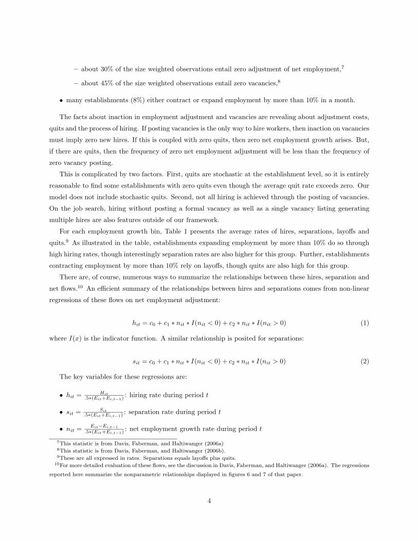
There are, of course, numerous ways to summarize the relationships between these hires, separation and

net flows.10 An efficient summary of the relationships between hires and separations comes from non-linear

regressions of these flows on net employment adjustment:

hit = c0 + c1 ∗ nit ∗ I(nit < 0) + c2 ∗ nit ∗ I(nit > 0) (1)

where I(x) is the indicator function. A similar relationship is posited for separations:

sit = c0 + c1 ∗ nit ∗ I(nit < 0) + c2 ∗ nit ∗ I(nit > 0) (2)

The key variables for these regressions are:

• hit = Hit

.5∗(Eit+Ei,t−1): hiring rate during period t

• sit = Sit

.5∗(Eit+Ei,t−1): separation rate during period t

• nit = Eit−Ei,t−1.5∗(Eit+Ei,t−1)

: net employment growth rate during period t

7This statistic is from Davis, Faberman, and Haltiwanger (2006a)8This statistic is from Davis, Faberman, and Haltiwanger (2006b).9These are all expressed in rates. Separations equals layoffs plus quits.

10For more detailed evaluation of these flows, see the discussion in Davis, Faberman, and Haltiwanger (2006a). The regressions

reported here summarize the nonparametric relationships displayed in figures 6 and 7 of that paper.

4

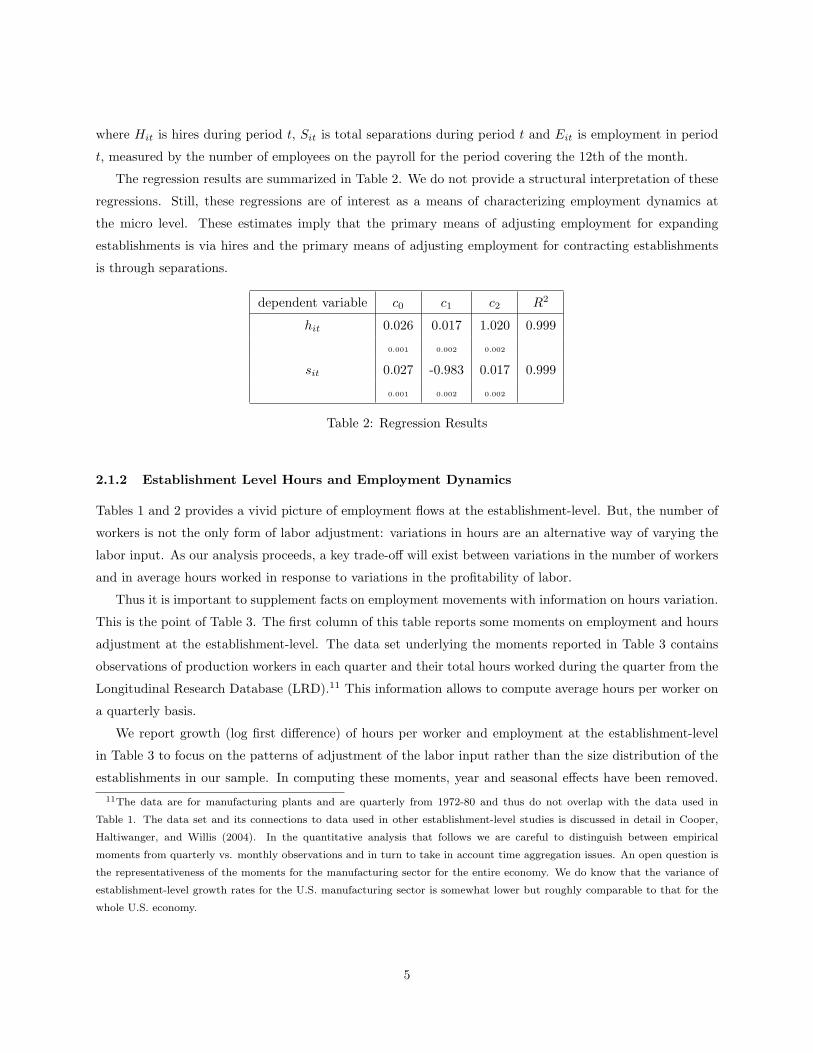
where Hit is hires during period t, Sit is total separations during period t and Eit is employment in period

t, measured by the number of employees on the payroll for the period covering the 12th of the month.

The regression results are summarized in Table 2. We do not provide a structural interpretation of these

regressions. Still, these regressions are of interest as a means of characterizing employment dynamics at

the micro level. These estimates imply that the primary means of adjusting employment for expanding

establishments is via hires and the primary means of adjusting employment for contracting establishments

is through separations.

dependent variable c0 c1 c2 R2

hit 0.026 0.017 1.020 0.999

0.001 0.002 0.002

sit 0.027 -0.983 0.017 0.999

0.001 0.002 0.002

Table 2: Regression Results

2.1.2 Establishment Level Hours and Employment Dynamics

Tables 1 and 2 provides a vivid picture of employment flows at the establishment-level. But, the number of

workers is not the only form of labor adjustment: variations in hours are an alternative way of varying the

labor input. As our analysis proceeds, a key trade-off will exist between variations in the number of workers

and in average hours worked in response to variations in the profitability of labor.

Thus it is important to supplement facts on employment movements with information on hours variation.

This is the point of Table 3. The first column of this table reports some moments on employment and hours

adjustment at the establishment-level. The data set underlying the moments reported in Table 3 contains

observations of production workers in each quarter and their total hours worked during the quarter from the

Longitudinal Research Database (LRD).11 This information allows to compute average hours per worker on

a quarterly basis.

We report growth (log first difference) of hours per worker and employment at the establishment-level

in Table 3 to focus on the patterns of adjustment of the labor input rather than the size distribution of the

establishments in our sample. In computing these moments, year and seasonal effects have been removed.11The data are for manufacturing plants and are quarterly from 1972-80 and thus do not overlap with the data used in

Table 1. The data set and its connections to data used in other establishment-level studies is discussed in detail in Cooper,

Haltiwanger, and Willis (2004). In the quantitative analysis that follows we are careful to distinguish between empirical

moments from quarterly vs. monthly observations and in turn to take in account time aggregation issues. An open question is

the representativeness of the moments for the manufacturing sector for the entire economy. We do know that the variance of

establishment-level growth rates for the U.S. manufacturing sector is somewhat lower but roughly comparable to that for the

whole U.S. economy.

5

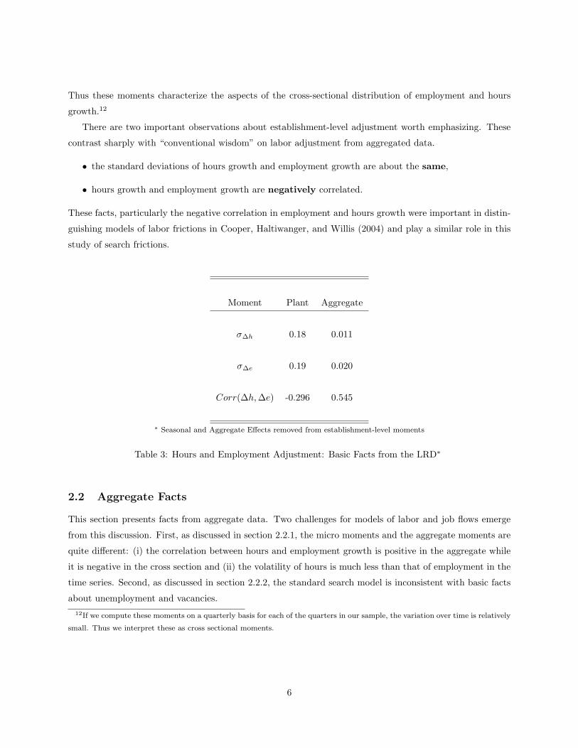
Thus these moments characterize the aspects of the cross-sectional distribution of employment and hours

growth.12

There are two important observations about establishment-level adjustment worth emphasizing. These

contrast sharply with “conventional wisdom” on labor adjustment from aggregated data.

• the standard deviations of hours growth and employment growth are about the same,

• hours growth and employment growth are negatively correlated.

These facts, particularly the negative correlation in employment and hours growth were important in distin-

guishing models of labor frictions in Cooper, Haltiwanger, and Willis (2004) and play a similar role in this

study of search frictions.

Moment Plant Aggregate

σ∆h 0.18 0.011

σ∆e 0.19 0.020

Corr(∆h,∆e) -0.296 0.545

∗ Seasonal and Aggregate Effects removed from establishment-level moments

Table 3: Hours and Employment Adjustment: Basic Facts from the LRD∗

2.2 Aggregate Facts

This section presents facts from aggregate data. Two challenges for models of labor and job flows emerge

from this discussion. First, as discussed in section 2.2.1, the micro moments and the aggregate moments are

quite different: (i) the correlation between hours and employment growth is positive in the aggregate while

it is negative in the cross section and (ii) the volatility of hours is much less than that of employment in the

time series. Second, as discussed in section 2.2.2, the standard search model is inconsistent with basic facts

about unemployment and vacancies.12If we compute these moments on a quarterly basis for each of the quarters in our sample, the variation over time is relatively

small. Thus we interpret these as cross sectional moments.

6

2.2.1 LRD Aggregate Job Flows

A second set of facts about aggregate data are in Table 3, in the second column. These data are obtained

by aggregating the plants in the LRD sample and computing moments from time series variation alone. The

contrast between the first and second columns is striking. For the aggregate data,

• the correlation of hours and employment growth is positive,

• the standard deviation of employment growth is almost twice that of hours growth.

One of the challenges for a model of labor adjustment is to explain the different pattern of the cross sectional

and time series moments in Table 3.

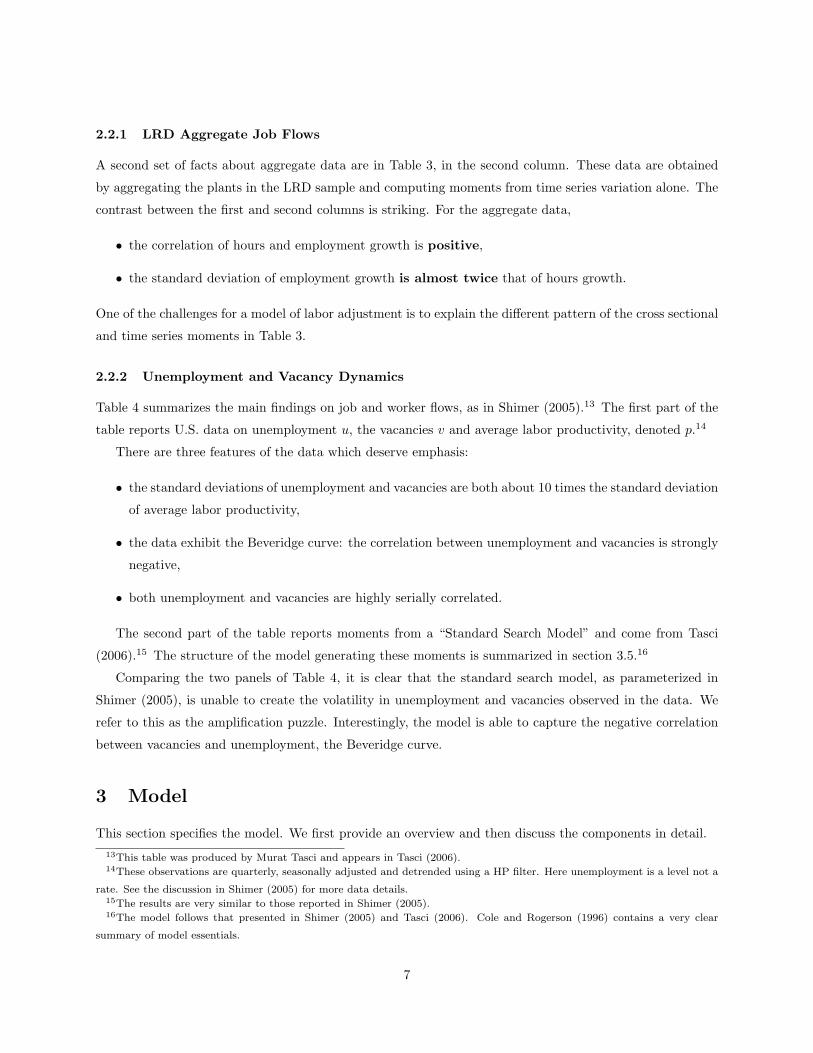
2.2.2 Unemployment and Vacancy Dynamics

Table 4 summarizes the main findings on job and worker flows, as in Shimer (2005).13 The first part of the

table reports U.S. data on unemployment u, the vacancies v and average labor productivity, denoted p.14

There are three features of the data which deserve emphasis:

• the standard deviations of unemployment and vacancies are both about 10 times the standard deviation

of average labor productivity,

• the data exhibit the Beveridge curve: the correlation between unemployment and vacancies is strongly

negative,

• both unemployment and vacancies are highly serially correlated.

The second part of the table reports moments from a “Standard Search Model” and come from Tasci

(2006).15 The structure of the model generating these moments is summarized in section 3.5.16

Comparing the two panels of Table 4, it is clear that the standard search model, as parameterized in

Shimer (2005), is unable to create the volatility in unemployment and vacancies observed in the data. We

refer to this as the amplification puzzle. Interestingly, the model is able to capture the negative correlation

between vacancies and unemployment, the Beveridge curve.

3 Model

This section specifies the model. We first provide an overview and then discuss the components in detail.13This table was produced by Murat Tasci and appears in Tasci (2006).14These observations are quarterly, seasonally adjusted and detrended using a HP filter. Here unemployment is a level not a

rate. See the discussion in Shimer (2005) for more data details.15The results are very similar to those reported in Shimer (2005).16The model follows that presented in Shimer (2005) and Tasci (2006). Cole and Rogerson (1996) contains a very clear

summary of model essentials.

7

U.S. DATA (Quarterly, 1951Q1-2003Q4)

u v v/u p

Std 0.19 0.20 0.38 0.02

Auto 0.94 0.95 0.95 0.89

Cross Correlations

u −0.89 −0.97 −0.42

v 0.97 0.37

v/u 0.40

Standard Search Model

u v v/u p

Std 0.01 0.02 0.03 0.02

Auto 0.85 0.74 0.81 0.81

Cross Correlations

u −0.87 −0.94 −0.94

v 0.99 0.99

v/u 0.99

For the data moments, the level of unemployment, u, is from the CPS, the level of vacancies, v, is from the Conference Board

and average labor productivity, p, is real output per person. These variables are seasonally adjusted and are log deviations

from an HP trend.

Table 4: Unemployment and Vacancies

3.1 Model Overview

There are two types of agents in the model: producers and workers. Producers operate production sites

which use labor as an input.17 The labor input is total hours and thus combines employees and the hours

each works. There are both aggregate and producer specific shocks which create revenue from the labor

input.

Workers and producers are brought together through a search process. A worker who is matched with a

producer has hours and compensation specified through a state contingent contract. The worker may lose

this job in a subsequent period, thus returning to a state of unemployment. Reflecting the search friction,

workers without a job are assumed to find a new job with some probability each period. This probability is

exogenous to the worker but is determined in equilibrium.17In this discussion, producers operate a production site and not a firm. This is consistent with our establishment level obser-

vations and assumes that firms with multiple establishments operate them independently, at least with respect to employment

decisions.

8

Producers have, at a point in time, a set of workers with whom they have a contract. In the short-run, the

producer responds to variations in a profitability shock, reflecting both productivity and demand, through

changes in hours worked per employee. The contract determines the response of hours and compensation to

the shock.

Producers also can create vacancies and hence change the number of employees. The process of creating

and filling vacancies entails adjustment costs. We allow for both fixed and variable costs of posting vacancies.

The presence of these fixed costs distinguishes our model from the existing search literature and defines the

boundaries of a producer. Empirically, these fixed costs are important to match observed inaction in the

adjustment of the number of workers.

With this structure in mind, we can reconsider the motivation for this exercise. The assumption that

producers have a fixed cost of posting vacancies will generate some inaction in vacancies and employment

adjustment. This is consistent with establishment-level evidence. Further, the observed negative correlation

between hours worked and the number of workers could reflect the inaction in posting vacancies. A producer

not hiring in the current period will response to higher demand for its product by increasing the hours of

its workers. But, once the producer decides to post vacancies and hires more workers, average hours worked

will drop.

From the perspective of matching moments on worker, job and unemployment flows as well as vacancies,

there are a couple of points to raise. First, the driving process for the model is establishment-specific

profitability. Various studies find that at the establishment-level productivity is considerably more variable

than in the aggregate. Thus, perhaps one resolution of the magnification problem highlighted in Shimer

(2005) is through the presence of volatile establishment-level shocks. The key is that, perhaps, these shocks

will create job and worker flows without increasing the measured variability of average labor productivity.18

As in Yashiv (2000), the model we consider has costs of adjusting the number of vacancies.19 As well

as creating inaction in vacancy creation and hiring, the non-convexity in adjustment may also increase the

volatility of job and worker flows.

3.2 Workers

In general, workers are in one of two states: employed or unemployed. If unemployed, the workers enjoy

leisure time. With a positive probability, they will be employed in the subsequent period.

Formally, the value of unemployment for a worker is given by:

V u = U(b) + β[f(u, v)EV e + (1− f(u, v))V u] (3)

18The mapping from a distribution of establishment-specific profitability shocks to an aggregate measure of average labor

productivity is likely to entail some smoothing through aggregation and by worker flows across producers.19Yashiv (2000) does not allow for non-convexity in the costs of vacancy creation and thus can estimate parameters from

Euler equations. His specification does include non-linearities in the adjustment costs.

9

where f(u, v) is the job finding rate which depends on the unemployment rate and the aggregate vacancy

rate. Here there is an expectations operator associated with V e since jobs with different producers may lead

to different values of employment. This could, in principle, be either due to heterogeneity in the contracts

or in the probability of retaining a job.

Employed workers have a contract for the current period which governs their state contingent compen-

sation and hours worked. In the following period there is a probability of losing their job and becoming

unemployed. For employed workers

V e = EεU(ω − g(h)) + β[(1− S)V e + SV u] (4)

where S is the separation (quits plus fires) rate.20

For the contracting process, assume producers make a take it or leave it offer to workers. This implies

that employed workers get no surplus: V e = V u = U(b)1−β . Therefore, in equilibrium, the value of employment

is independent of the producer with whom the worker has a job. Thus the expectations operator in (3) is

not necessary. Since workers are risk averse and get expected utility of V u, the contracted compensation

and hours, (ω, h), must lie along an indifference curve given by U(ω − g(h)) = U(b).

This assumption of giving producers all of the bargaining power immensely simplifies the analysis since

workers do not care which producer they work for. Otherwise, the different producers would offer different

terms and have different retention probabilities and workers would have to keep track of the entire distribution

of producers.

Interestingly, producer heterogeneity is present in compensation levels, and hours will still reflect producer

specific state variables and shocks. So there will be a non-degenerate cross sectional distribution of (ω, h)

but a degenerate cross sectional distribution of utility levels.

3.3 Producers

Producers have access to a technology which creates output from labor input. The revenue function is given

by:

aε(eh)α (5)

where a is the aggregate (profitability) shock, ε is the producer specific shock and total labor input is the

product of the number of workers, e, and hours per worker, h. We allow for curvature in the revenue function,

parameterized by α, which may capture diminishing returns to scale due to fixed factors of production

excluded (5).21

20This value may be producer specific but is ignored in the notation.21It is tempting as well to interpret α as capturing market power but, strictly speaking, this is not consistent with the

structure of the model.

10

We assume two stages in the producer’s problem. First, given the aggregate state, the producer contracts

with its workers. Second, ex post, the establishment specific shock is realized and state contingent hours are

determined given the contract.

3.3.1 Setting a Contract

A contract is δ = (ω(s), h(s)) for all s, where s = (a, ε, e) is the establishment’s state, ω(s) is compensation

and h(s) is hours worked. The contract allows compensation and hours to be fully state contingent. In

terms of timing, the contract is determined given (a, e) but prior to the determination of ε. This timing is

consistent with the literature on risk sharing through labor contracts and is important for matching moments

on relative employment and hours variability. All workers with a given producer get the same contract since

they are identical and have the same outside option of unemployment.

The producer selects the contract to solve

π(a, e) = maxδEε[aε(eh(s))α − eω(s)] (6)

where the expectation is over the idiosyncratic component of profitability. The constraint is that the expected

utility from the contract not be less than the outside option of unemployment, V u:

V e(a, e) = EεU(ω(s)− g(h(s))) + βE[(1− S)V e + SV u] ≥ V u (7)

where V e is the value of being employed next period and V u is the value of being unemployed next period.

Assuming this constraint binds, then V e = V u equals the value of leisure in equilibrium, U(b). Given the

risk aversion of the workers, optimal risk sharing implies that marginal utility is constant. Thus compensation

and hours will satisfy the condition

U(ω(s)− g(h(s))) = U(b) (8)

for all s.

3.3.2 Determining Hours

Once ε is realized, hours are determined by the contract. With (8) holding for all s, workers are fully

compensated for hours variations. So the optimal hours choice is easy to characterize. Given (a, e, ε), the

producer chooses a level of hours subject to the worker getting utility U(b), i.e. ω = g(h) + b. Solving this

sub-problem guarantees that the worker receives a constant level of utility, U(b). The optimization problem

for hours is

maxhaε(eh)α − eg(h)− eb (9)

11

which implies h(a, e, ε). The hours choice satisfies

αaε(eh)α−1 = g′(h). (10)

This first order condition generates a policy function for hours which depend on (a, e, ε). Holding (a, ε)

fixed, as e increases, it is clear that h falls. This will be relevant later as we try to match a negative correlation

in observed hours and employment growth at the establishment.

3.3.3 Determining the level of Employment

The level of employment is determined by vacancy posting decision of the producer.22 The recruiting decision

is made knowing s ≡ (a, e−1, ε−1) where e−1 is the inherited stock of workers and ε−1 is the shock last period

used to predict the current one. The state vector s is similar to s except for the timing of decisions on e and

the realization of the idiosyncratic profitability shock.

Q(s) is the value of the establishment in state s and is given by

Q(s) = max{Qh(s), Qn(s), Qf (s)} (11)

where Qh(s), Qn(s) and Qf (s) relate to the hiring, no-adjustment and firing options.

The value of hiring workers is given by

Qh(s) = maxvEe,επ(a, ε, e)− F+ − C+(v) + βEQ(s′) (12)

When the producer posts v vacancies, the evolution of employment is

e = e−1(1− q(u, v)) + H(u, v)v (13)

where q(·) is the quit rate and H(·) is the rate at which a vacancy is filled. In this formulation, both the quit

rate and the vacancy filling rate depend on u, the unemployment rate, and v, the aggregate vacancy rate.

Given the aggregate state of the economy, H(·) and q(·) are deterministic from the producer’s viewpoint.

That is, stochastic aspects of the matching process and quits are not part of the uncertainty facing a producer.

There are two types of costs of posting vacancies in the model. There is a fixed cost component, F+,

and a variable cost component, C+(v). There is the familiar interpretation of this type of specification

based upon recruiting in Economics. The fixed cost appears in the form of reading numerous files, flying a

committee to interview and so forth. The variable cost is related to the number of interviews and fly-outs.

In terms of matching the moments, these two costs are relevant for capturing inaction, through F+, and

partial adjustment, through C+(v).

The value of firing workers is given by

Qf (s) = maxfEεπ(a, ε, e−1(1− q(u, v))− f)− F− − C−(f) + βEQ(s′). (14)

22Here vacancies must be reposted each period. See Fujita and Ramey (2005) for a model where vacancies are a state variable.

12

Here the level of employment reflects quits and fires. There are fixed, F−, and variable costs, C−(f), of

firing workers.

The value of inaction is given by

Qn(s) = Eεπ(a, ε, e−1(1− q(u, v))) + βEQ(s′). (15)

Here inaction means no hiring and no firing so that employment at the establishment level will fall due to

quits.

Firms discount at the same rate as private agents. This is a consequence of the fact that consumption

in all states is b so that the worker’s Euler equation would imply β(1 + r) = 1, where r is the real interest

rate. Hence the producers discount at rate β.

We assume that any profits realized by producers are consumed by entrepreneurs who own the production

process. At this point of the analysis, there is no free entry.

3.4 Equilibrium

An equilibrium for this economy requires optimization by producers and workers and consistency conditions.

For optimization, the components of an equilibrium are:

• An optimal labor contract which solves (6) subject to the participation constraint of the workers,

• A state contingent hours schedule which solves (10),

• A decision rule for employment adjustment which solves (11),

• A decision rule for workers’ entailing acceptance or rejection of the contract, as in (7).

With regards to the consistency conditions, a constraint in the optimization problem of the producers,

(13), includes two functions which depend on aggregate variables: the quit function, q(u, v), and the matching

function, m(u, v). These functions, which are taken as given in the optimization problem of the producer,

must be consistent with the relationships generated by the model and the data.

Finally, the unemployment rate follows u′ = (1− u)S(u, v)+(1−f(u, v))u where S(u, v) is the separation

rate (quits plus layoffs) and f(u, v) is the job finding rate. In equilibrium, 0 ≤ u ≤ 1. As all workers

are either employed or unemployed in our model, we use the transition equation for total employment to

generate an unemployment series to evaluate the moments reported in Table 4.

3.5 Comparison to Standard Search Model

Section 2.2.2 discusses key moments of worker flows and, following Shimer (2005), points to key differences

between the data and the standard search model. Here we briefly outline the standard search model relative

to the model we consider. This discussion draws upon Shimer (2005) and Tasci (2006).

13

There are a couple of key differences between the models. The standard search model assumes each

producer has at most one worker. Firms without a worker post a vacancy at a (flow) cost and that vacancy

is either filled or not.

Further, there is no movement on the intensive margin in the standard model. That is, variations in hours

are not studied and thus there is no state contingent contract governing the response of hours to shocks. So

matching hours variations is not possible.

Shocks in the standard model are common across producers.23 Thus the models are not equipped to

match cross sectional observations.

The standard model does contain a more interesting analysis of the bargaining problem. For the moments

in Table 4, the bargaining weight for workers was set at 0.72.24

Once workers have a share of the surplus, then the utility flow during a period of unemployment, para-

meterized by b, becomes more important to the analysis. Shimer (2005) assumes a value of leisure at 40%

of average productivity. Hagedorn and Manovskii (2006) take a more general view of the value of leisure

beyond the replacement rate from unemployment insurance and, by matching moments of labor flows and

the elasticity of wages with respect to productivity variations, set b = 0.955 and the bargaining share of

workers at only 0.05. As seen in their Table 4, this parameterization resolves the problem of the relative

standard deviation of unemployment and vacancies.

In many respects, the optimal contracting structure along with the bargaining power held by producers

we explore in our model is much closer to the parameterization of Hagedorn and Manovskii (2006). We have

given the producer all of the bargaining power so that the workers have a zero weight. Further, the optimal

contract stabilizes worker’s ex post utility at the value of leisure. This is very much like a value of b = 1.

The property that workers receive insurance over employment status is a common feature of optimal

contracting models.25 In our model, we allow work sharing so that hours vary. Hence, there are no ex

post employment variations within a period and thus inclusion of unemployment insurance in the optimal

contract does not arise.

Also, the fact that the utility flow to workers is determined by the fixed value of leisure generates a form

of wage stickiness as in Hall (2005). Of course, this property of our model reflects the optimal insurance

features of the labor contract. Further, wages per se are not allocative in our framework. Instead, hours

respond to the state and satisfy (10) and compensation adjusts so that utility is equal to U(ω−g(h)) = U(b)

ex post. Thus the model has implications for the cross sectional distributions of hours and compensation

which we do not exploit.

Finally, the standard model has a free entry condition which pins down the value of a vacancy at zero.

Instead, we have producers optimally choosing the number of vacancies to post. Our focus is more on the23Mortensen and Pissarides (1994) did have job specific shocks which they use to generate job destruction. Cole and Rogerson

(1996) also allowed for idiosyncratic shocks but then found that these shocks did not have aggregate effects.24See Shimer (2005) and Hagedorn and Manovskii (2006) for a discussion of the parameterization of the bargaining weight.25See Azariadis (1975) for details as well as a model in which there are unemployment risks due to the absence of severance

pay and no work sharing.

14

intensive margin of adjustment in the number of vacancies per producer rather than the number of producers.

4 Numerical Analysis

The optimization problem for an individual producer is solved through value function iteration of (11) and

the functions used to define this value. There is no household optimization to consider: as long as V e = V u

workers are indifferent between accepting a job or not.

There is an equilibrium component to consider since the value of the problem to the producer depends

on the matching function which, in turn, depends on the choices of the other producers in the economy. This

is clear from (12) where the value of hiring workers depends on the matching function which has aggregate

variables as arguments.

Instead of computing an equilibrium, we impose these conditions in our estimation. More precisely,

we estimate from the data the relationship between the hiring rate and aggregate variables. We use those

estimated parameters in the producer optimization problem. Then, we make sure the estimated model

reproduces the empirical relationship between match rates and aggregate variables. In this way, the beliefs

of the individual producers about the dependence of the match rate on aggregate variables is consistent with

both the model and data.

To solve the producer’s optimization problem, we need a number of parameterized functions. We discuss

the functions here and then summarize them, along with parameterizations in Table 5. We specify and

parameterize the model at a monthly frequency. Thus the moments associated with worker flows are not

time aggregated.

4.1 Functional Forms

As argued above, the wage, ω(s) will satisfy U(ω(s)−g(h(s)) = U(b) for all s. We parameterize the disutility

of work, g(h) so that

ω = b + ω1hζ (16)

is the compensation function required to guarantee the utility level U(b) in all states. Here ζ is important

for determining the utility cost of variations in hours. Generally, if ζ is low, then variations in hours are

inexpensive so that much of the adjustment of the labor input will be on the intensive margin and not in

through variations in the number of workers.

For the hiring and firing of workers, we assume that the variable cost of vacancies is given by C(v) =

c+0 vc+

1 . The variable cost of firing workers is similarly parameterized, C(f) = c−0 fc−1 .

Following the literature, the matching function is constant returns to scale and is given by

m = µuγ v1−γ = µvθ−γ (17)

15

where θ ≡ vu is measures the tightness of labor markets. From this relationship, we obtain two additional

functions: the vacancy filling rate for producers and the job finding rate for workers. Let H = mv be the

vacancy filling rate. Using the specification of the match rate, (17),

H = µθ−γ . (18)

Let f = mu be the job finding rate for workers. Using (17) again,

f = µθ1−γ . (19)

Of course, these three functions are related by common parameters.

As noted above, quits are allowed to depend on the state of the labor market. We assume

q = q0θq1 . (20)

A positive value of q1 means that as the vacancy-unemployment ratio increases, quits increase as well.

Finally, we impose a relationship between the vacancy-unemployment ratio (θ) and the aggregate state

of productivity, measured as average labor productivity and denoted p, relative to its mean,(

pp

),

θ = θ0

(p

p

)θ1

. (21)

These relationships play two roles in our study. First, for the numerical analysis we solve the producer’s

dynamic optimization problem given these (parameterized) relationships. There is no equilibrium analysis

at this stage. We simply study the solution of the producer’s problem given the evolution of the aggregate

variables, (a, θ). In particular, the state vector for the producer includes the common component of aggregate

productivity, a.

Through (21), we can relate labor market tightness, θ, to the state of aggregate productivity. We

substitute this relationship into equations (17), (20), (18) and (21) to link these rates to a. In practice, it is

sufficient to relate H(·) directly to a in the model:

H = ν0aν1 . (22)

Given ν0, ν1, the producer can solve its dynamic optimization problem directly. If a was the same as average

labor productivity, then using (21) and (18), ν1 = −γθ1.

While using (22) is an approximation, it allows us to significantly reduce the state space of the producer’s

problem. So, when the producer solves its dynamic optimization problem, it uses the current value of

aggregate productivity to forecast the future value of aggregate productivity and hence future labor market

tightness and thus the vacancy filling rate for the future.

Second, part of our quantitative exercise focuses on estimating the parameters of these functions on

simulated data. This imposes consistency between the beliefs of the producers, the actual data and the

16

relationships generated by the simulated data. In equilibrium, the producer’s beliefs will be consistent with

actual and simulated data. We impose this condition in the estimation procedure.

To understand the procedures we use, suppose the aggregate component of profitability, a, was observable.

Then we would estimate H(a) from the data and impose this relationship in the producer’s optimization

problem. In this way, producer’s beliefs about the matching process would be consistent with the data and

thus with the matching relationship within the model.26

However, we do not have a measure of a. So instead, we estimate (18) from the data and require, as a

moment matching condition, that this relationship be reproduced in the simulated data of our model. In

this manner, the consistency requirement of equilibrium becomes a moment condition used to set ν1 and

other parameters.27

4.2 Estimated Functions

This section reports our estimates of the parameters for three functions. This estimation is done directly

from the data and is thus outside of the solution of the producer’s dynamic optimization problem.

For this analysis as well as the estimation, we construct a monthly vacancy series using JOLTS. The

monthly unemployment data is from the CPS. Relative to Shimer (2005), our data are higher frequency and

we use the JOLTS vacancy series. For monthly labor productivity, we construct a series using the Industrial

Production Index from the FRB and total hours using employment and hours data from the BLS. Labor

market tightness, θ, is the log of the vacancy-unemployment ratio. All series are converted to logs and then

HP filtered.

The results are reported in Table 5. The first relationship relates labor market tightness, ln(θ), to

departures of aggregate productivity from average,(

pp

). The constant in this regression provides an estimate

of the average value of labor market tightness of 0.46.

The parameter estimate of θ1 = −9.12. Labor market tightness is countercyclical in our data: when

productivity is above average, labor markets are relatively lose. This appears at variance with the positive

comovement between labor market tightness and productivity reported in Shimer (2005). However, as

reported in footnote 10 of that paper, the correlation is very unstable over time and for the last years of his

sample is negative as well.

The next estimated relationship is the matching function, where the logarithm of the match rate is

regressed on the logarithm of labor market tightness. In keeping with a large part of the literature we

impose constant returns to scale. With this restriction we estimate γ = 0.36, which is considerably lower

than the estimate of 0.72 reported in Shimer (2005) and closer to the estimate of 0.235 reported in Hall

(2005). The difference in estimates may reflect rest the use of the JOLTS data rather than the Conference

Board vacancies numbers and the different sample periods.26Since a is an exogenous process, this second requirement is trivial. In fact, once we work with H(a) directly, the optimization

problem of the establishment are not related.27See Willis (2003) for a related application of this approach.

17

Relationship Estimate standard error

Relating Labor Tightness to Productivity(21)

ln(θ0) -0.8435 0.022

θ1 -12.41 1.546

R2 0.5056

Vacancy Filling as a function of labor market tightness (18)

µ 1.0072 0.02

γ 0.3581 0.02

R2 0.7651

Quits as a function of labor market tightness (20)

ln(q0) -3.76 0.0172

q1 0.3169 0.0204

R2 0.7937

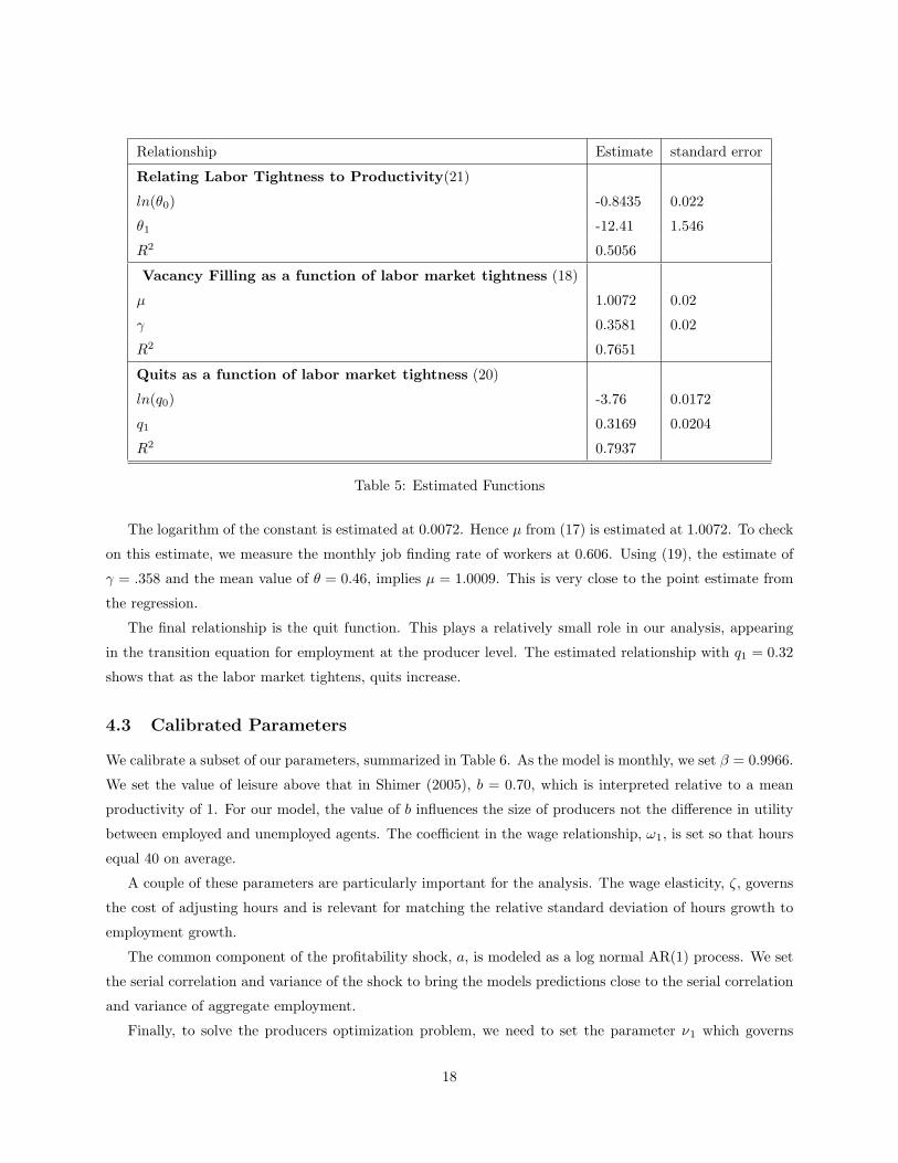
Table 5: Estimated Functions

The logarithm of the constant is estimated at 0.0072. Hence µ from (17) is estimated at 1.0072. To check

on this estimate, we measure the monthly job finding rate of workers at 0.606. Using (19), the estimate of

γ = .358 and the mean value of θ = 0.46, implies µ = 1.0009. This is very close to the point estimate from

the regression.

The final relationship is the quit function. This plays a relatively small role in our analysis, appearing

in the transition equation for employment at the producer level. The estimated relationship with q1 = 0.32

shows that as the labor market tightens, quits increase.

4.3 Calibrated Parameters

We calibrate a subset of our parameters, summarized in Table 6. As the model is monthly, we set β = 0.9966.

We set the value of leisure above that in Shimer (2005), b = 0.70, which is interpreted relative to a mean

productivity of 1. For our model, the value of b influences the size of producers not the difference in utility

between employed and unemployed agents. The coefficient in the wage relationship, ω1, is set so that hours

equal 40 on average.

A couple of these parameters are particularly important for the analysis. The wage elasticity, ζ, governs

the cost of adjusting hours and is relevant for matching the relative standard deviation of hours growth to

employment growth.

The common component of the profitability shock, a, is modeled as a log normal AR(1) process. We set

the serial correlation and variance of the shock to bring the models predictions close to the serial correlation

and variance of aggregate employment.

Finally, to solve the producers optimization problem, we need to set the parameter ν1 which governs

18

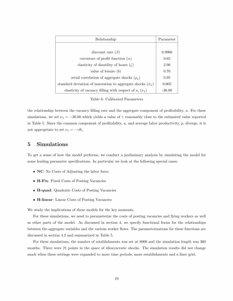
Relationship Parameter

discount rate (β) 0.9966

curvature of profit function (α) 0.65

elasticity of disutility of hours (ζ) 2.90

value of leisure (b) 0.70

serial correlation of aggregate shocks (ρa) 0.95

standard deviation of innovation to aggregate shocks (σa) 0.005

elasticity of vacancy filling with respect of a, (ν1) -30.00

Table 6: Calibrated Parameters

the relationship between the vacancy filling rate and the aggregate component of profitability, a. For these

simulations, we set ν1 = −30.00 which yields a value of γ reasonably close to the estimated value reported

in Table 5. Since the common component of profitability, a, and average labor productivity, p, diverge, it is

not appropriate to set ν1 = −γθ1.

5 Simulations

To get a sense of how the model performs, we conduct a preliminary analysis by simulating the model for

some leading parameter specifications. In particular we look at the following special cases:

• NC: No Costs of Adjusting the labor force.

• H-Fix: Fixed Costs of Posting Vacancies

• H-quad: Quadratic Costs of Posting Vacancies

• H-linear: Linear Costs of Posting Vacancies

We study the implications of these models for the key moments.

For these simulations, we need to parameterize the costs of posting vacancies and firing workers as well

as other parts of the model. As discussed in section 4, we specify functional forms for the relationships

between the aggregate variables and the various worker flows. The parameterizations for these functions are

discussed in section 4.2 and summarized in Table 5.

For these simulations, the number of establishments was set at 8000 and the simulation length was 360

months. There were 21 points in the space of idiosyncratic shocks. The simulation results did not change

much when these settings were expanded to more time periods, more establishments and a finer grid.

19

5.1 Key Points

The simulation exercise is structured around three key moments from the data. These moments are of

interest partly because they are associated with empirical puzzles. Here we discuss these key moments and

then we study how our model addresses them below.

The first of these is summarized in Table 4. The standard deviation of unemployment relative to aggregate

labor productivity as well as the the standard deviation of vacancies relative to aggregate labor productivity

is considerably smaller in the model than in the data. This is an amplification puzzle.

The second key moment is the observed negative correlation between employment and hours growth at

the establishment-level, as indicated in Table 3. As discussed in Cooper, Haltiwanger, and Willis (2004),

this correlation is positive in aggregate data.

The third set of moments of interest are summarized in Table 1. The cross sectional distribution of net

employment growth indicates both substantial inaction as well as bursts of job creation and destruction.

The challenge is to find a model capable of matching these disparate observations from micro and ag-

gregate data. As illustrated in the simulations below, our model’s inclusion of non-convex costs of vacancy

creation along with substantial dispersion in establishment-specific shocks provides a basis for matching

these moments.

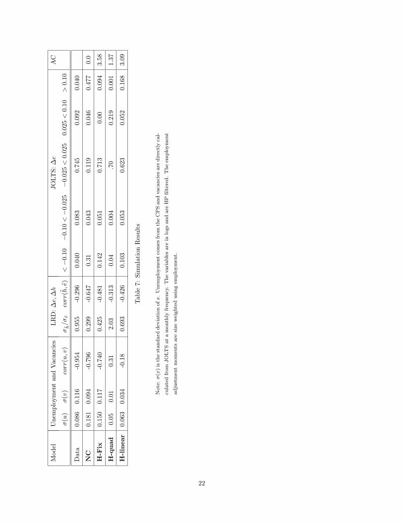
5.2 Simulation Results

Table 7 presents the main moments of interest for the cases listed above. Almost all of these moments are

calculated on a monthly basis, the same frequency we observed most of the data. The exception are the two

quarterly moments from the LRD, σh/σe and corr(h, e), which are calculated for a each quarter by sampling

from the simulated monthly data.

The first specification, NC, has no costs of hiring and firing. The consequence of this is substantial

volatility in unemployment, matching and job finding, relative to the other cases. In contrast, there is

relatively little variability in vacancies. This difference in variability of unemployment relative to vacancies

reflects the fact that unemployment is a state variable. The model does generate a Beveridge curve.

Still, due to the assumption that hours but not employment responds immediately to the idiosyncratic

shock, adjustment of both hours and employees occurs. But, without adjustment costs, much of the variation

is in the form of employment growth so σh/σe is much higher in the data than the model. Interestingly, the

model without adjustment costs can reproduce the negative corr(h, e) in the data. This finding is explained

below.

Looking at employment adjustment, it is clear that in the absence of adjustment costs, the volatility

of employment growth at the establishment level is excessive relative to observation. In the simulation it

is not uncommon to see employment growth, in absolute value, in excess of 10%. This finding should not

be surprising given the volatility of the idiosyncratic shocks. Clearly a key issue in the estimation will be

the identification of the costs of creating vacancies and the other adjustment costs from the variance of the

20

idiosyncratic shocks.

Relative to these results, the introduction of costs of posting vacancies and firing are relevant for reducing

the variability of job and worker flows. There are a couple of cases summarized in Table 7 depending on

whether hiring or firing costs are present.

The H-fix specification introduces a fixed cost, F+ = 1, into the model. At this value of F+, the average

adjustment cost incurred, given in the “AC” column, is about 3.6% of monthly gross profits (revenues less

compensation to workers). With this relatively high adjustment cost, there is relatively more inaction, i.e.

more employment growth in the (−2.5, 2.5) bin of the employment distribution and less frequent bursts of

job creation and destruction. Further, the distribution of employment growth is skewed: there are few small

positive employment growth rates but more small negative employment growth rates. In this sense, the

adjustment cost alters the distribution of employment variation.

The Beveridge curve is still present in the simulated data. The fixed cost increases the variability of

unemployment and of vacancies, relative to the no-adjustment cost case. There is a negative correlation

between hours and employment growth at the establishment-level and employment growth remains more

variable than hours growth.

The H-quad specification introduces a quadratic cost of posting vacancies, c+0 = 0.05, c+

1 = 2, F+ = 0.

At these parameter values the adjustment costs are about 1.37% of gross profits.28 The distribution of

employment changes is now concentrated in the (−2.5, 2.5) interval. In contrast to the H-fix case, where

96% of the observations had zero vacancies posted, here the small adjustment of employment reflects the

traditional partial adjustment structure. In this case we find zero employment growth in only about 20%

of the observations as producers choose to incur the relatively small adjustment costs to offset quits even

when profitability is not changing. Clearly, the interaction of adjustment costs and the distribution of the

idiosyncratic shocks have a big impact on the distribution of employment changes.

With these adjustment costs the Beveridge curve is gone: the correlation between unemployment and

vacancies is positive. Further, the standard deviation of vacancies is quite small. With quadratic adjustment

costs, employment growth is not too variable so that the standard deviation of hours growth relative to

employment growth is about 2.0.

28At a higher adjustment cost so that these costs are 3.5% of gross profits, the distribution of employment growth was

degenerate with all of the weight in the middle bin. This is not an interesting case to study.

21

Mod

elU

nem

ploy

men

tan

dV

acan

cies

LR

D:∆

e,∆

hJO

LTS:

∆e

AC

σ(u

)σ(v

)co

rr(u

,v)

σh/σ

eco

rr(h

,e)

<−

0.10

−0.

10<−

0.02

5−

0.02

5<

0.02

50.

025

<0.

10>

0.10

Dat

a0.

086

0.11

6-0

.954

0.95

5-0

.296

0.04

00.

083

0.74

50.

092

0.04

0

NC

0.18

10.

094

-0.7

960.

299

-0.6

470.

310.

043

0.11

90.

046

0.47

70.

0

H-F

ix0.

150

0.11

7-0

.740

0.42

5-0

.481

0.14

20.

051

0.71

30.

000.

094

3.58

H-q

uad

0.05

0.01

0.31

2.03

-0.3

130.

040.

004

.70

0.21

90.

001

1.37

H-lin

ear

0.06

30.

034

-0.1

80.

693

-0.4

260.

103

0.05

30.

623

0.05

20.

168

3.09

Tab

le7:

Sim

ulat

ion

Res

ults

Note

:σ(x

)is

the

standard

dev

iati

on

ofx.

Unem

plo

ym

entco

mes

from

the

CP

Sand

vaca

nci

esare

dir

ectly

cal-

cula

ted

from

JO

LT

Sat

am

onth

lyfr

equen

cy.

The

vari

able

sare

inlo

gs

and

are

HP

filter

ed.

The

emplo

ym

ent

adju

stm

ent

mom

ents

are

size

wei

ghte

dusi

ng

emplo

ym

ent.

22

The H-linear specification introduces a linear cost of posting vacancies: c+0 = 0.5, c+

1 = 1, F+ = 0. As

with the H-fix specification, the adjustment cost is around 3.0%. Relative to the H-fix case, the variability of

unemployment and vacancies is much lower. The Beveridge curve is still present as is the negative correlation

between hours and employment growth. Relative to the H-quad case, there are again observations of large

job creation. This case also yields a more symmetric distribution of net employment growth. This form of

adjustment cost implies zero vacancies posted in about 60% of the observations.

5.3 Inspecting the Mechanism

This is a rather rich model and the mapping from parameters to moments is not immediately clear. To help

build further intuition about the models mechanics, we explore in more detail the specification with a fixed

costs of posting vacancies, labeled H-fix in Table 7. We do so here by presenting two figures related to key

moments.

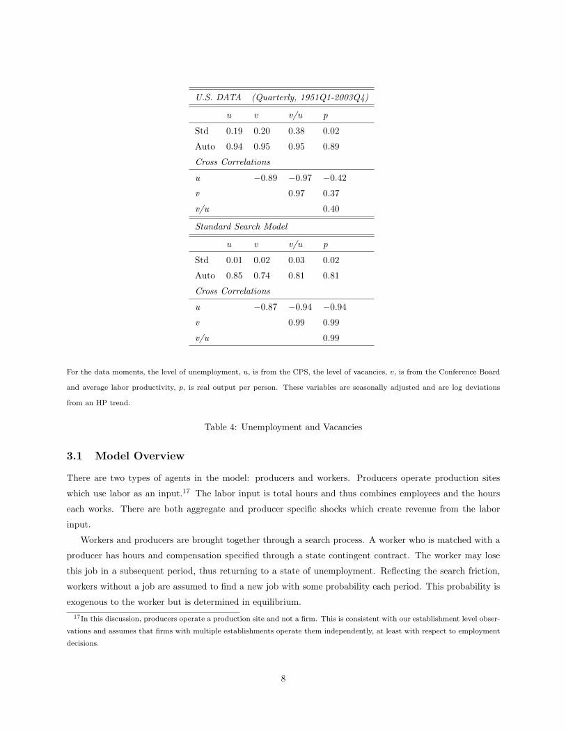
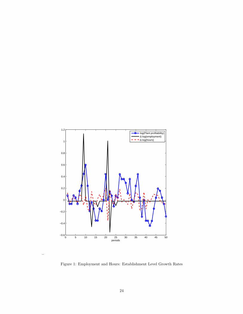
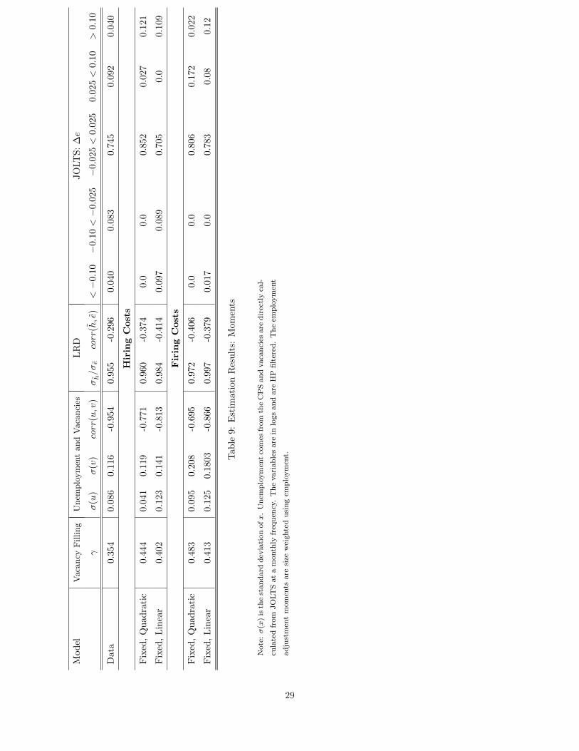
Figure 1 shows simulation results at the establishment level. The point here is to understand how an

establishment, in the presence of fixed and variable costs of posting vacancies, responds to variations in

profitability.

Two points are illustrated in Figure 1. First, hours and employment are negatively correlated. When the

producer is subject to an increase in profitability, starting in period 7 in Figure 1, hours respond immediately.

In period 8, the adjustment cost is paid and employment adjusts to a higher level. Hours are reduced as

employment expands and this produces the negative correlation between hours and employment growth.

Second, due to the adjustment costs, employment does not always respond to variations in profitability.

This is evident from period 26 onward in Figure 1. Though profitability has risen in this period, there is no

employment response. Instead, fluctuations in profitability are met by variations in hours. Thus variations

in adjustment are sporadic.

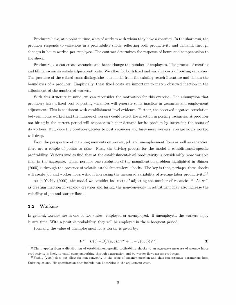
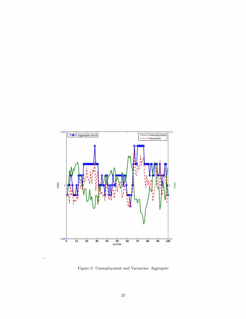
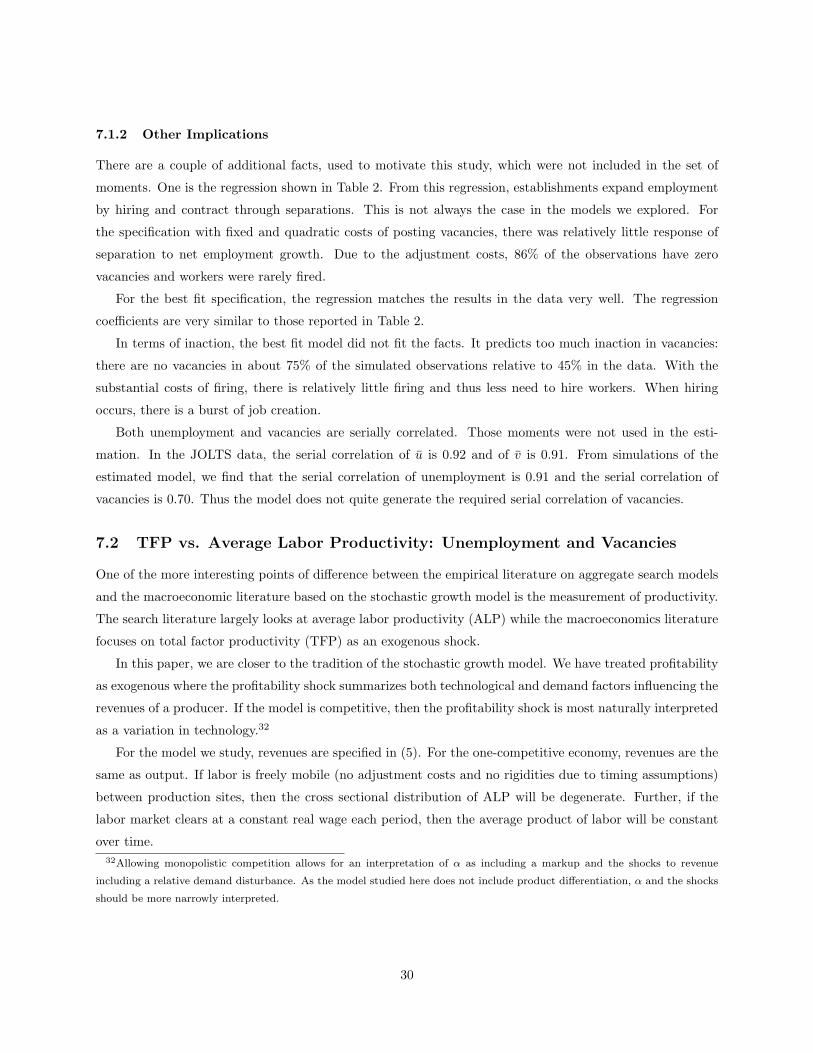
Figure 2 shows simulation results for unemployment, vacancies and the aggregate component of the

profitability shock. These aggregate variables are obtained by the aggregation of the establishment level

results for the same simulation shown in Figure 1.

The Beveridge curve is apparent in these simulations. When there is a positive aggregate shock, such

as around period 27, there is an immediate response in the creation of vacancies. Unemployment falls as

vacancies are filled. The strength of this response depends partly on the cost of creating vacancies and on

the rate in which vacancies are filled.

Notice too that there appears to be no magnification puzzle in the simulated data.29 The variability of

the aggregate component of profitability, measured on the left axis, is quite small relative to the variability

of unemployment and vacancies, measured on the right axis.

There are inherent differences in the dynamics of the response of unemployment and vacancies to the29To be careful though, the magnification issue relates aggregate average labor productivity not aggregate profitability to

variations in u and v.

23

..

0 5 10 15 20 25 30 35 40 45 50−0.6

−0.4

−0.2

0

0.2

0.4

0.6

0.8

1

1.2

periods

log(Plant profitability)∆ log(employment)∆ log(hours)

Figure 1: Employment and Hours: Establishment Level Growth Rates

24

..

0 10 20 30 40 50 60 70 80 90 1000.99

1

1.01

inde

x

periods

0 10 20 30 40 50 60 70 80 90 1000.5

1

1.5

inde

x

Aggregate shock Unemployment

Vacancies

Figure 2: Unemployment and Vacancies: Aggregate

25

shock. In most of these search and matching models, unemployment is a state variable but vacancies are

not.30 As reported in Table 4 the serial correlations of unemployment and vacancies are about the same. As

is evident from Figure 2, the serial correlation of vacancies created by the model is substantially less than

the serial correlation of unemployment.

6 Estimation

The key parameters in our study are those determining the costs of hiring and firing as well as the driving

process for the shocks at the establishment-level. These parameters are estimated through a simulated

method of moments procedure. Other parameters are calibrated at the values in Table 6.

6.1 Methodology

The estimation entails finding the vector of structural parameters, Λ, to minimize the (weighted) distance

between moments from the data, Γd, and moments produced from a simulation of the model given a vector

of parameters, Γs(Λ). Thus our estimate of Λ minimizes £(Λ) where

£(Λ) ≡ (Γd − Γs(Λ))W (Γd − Γs(Λ))′ (23)

and W is a weighting matrix.31

This minimization problem is solved by simulation to create a mapping from Λ to the moments. The

methodology is as follows. Given vector Λ, solve the producer’s dynamic optimization problem using value

function iteration. From this and the solution to (10), we generate policy functions at the producer level for

employment, vacancies and hours. The model is solved at a monthly frequency. Using these policy functions,

we create a simulated data set at the producer level. Given this, we can compute the microeconomic moments

directly from the data and, by aggregation, compute aggregate flows of vacancies and unemployment as well.

In this manner, we obtain Γs(Λ).

The simulated data set consists of 8000 establishments simulated over 360 months. The results are

robust to increasing the number of establishments and time periods. The number of points in the grid for

the idiosyncratic shock was 21.

For our analysis, the parameter vector we estimate includes: Λ = (F+, c+0 , F−, c−0 , ρε, σε, ν1, ). The first

three parameters represent the cost of posting vacancies and the second three are firing costs. The parameters

(ρε, σε) characterize the log normal AR(1) process for the establishment-specific profitability shocks. The

final parameter, ν1, captures producer’s beliefs about the response of the matching rate to variations in

aggregate profitability.

We separate the moments to match into four categories:30As noted earlier, one exception is Fujita and Ramey (2005).31In the discussion which follows, W is an identity matrix which produces consistent estimates of Λ.

26

• Equilibrium: The estimated model must mimic the regression results for the vacancy filling rate in

(18). Here we focus on the elasticity of vacancy filling with respect to labor market tightness, γ

• Unemployment and Vacancies: The key moments are std(u) and std(v) and corr(u, v). The

moments are reported in Table 7.

• Hours and Employment: The key moments are corr(∆e,∆h) and std(∆e)std(∆h) . These are in terms of

growth rates and are measured in the data and simulation quarterly as reported in Table 3 for the

establishment-level.

• Worker and Job Flows: The key moments are from the distribution of ∆e reported in Table 1.

These moments are chosen largely because they characterize basic aspects of worker and job flows at

both the microeconomic and aggregate levels. This is in accord with the point of our analysis: to investigate

a search model capable of jointly explaining both microeconomic and macroeconomic facts.

6.2 Results

The estimation is undertaken for four cases: two with hiring costs and two with firing costs. Each of the two

hiring cost specifications included a fixed cost of vacancies in conjuction with either a quadratic or linear

cost of vacancies. Each of the two firing cost cases included a fixed cost of firing in conjuction with either a

quadratic or linear firing cost.

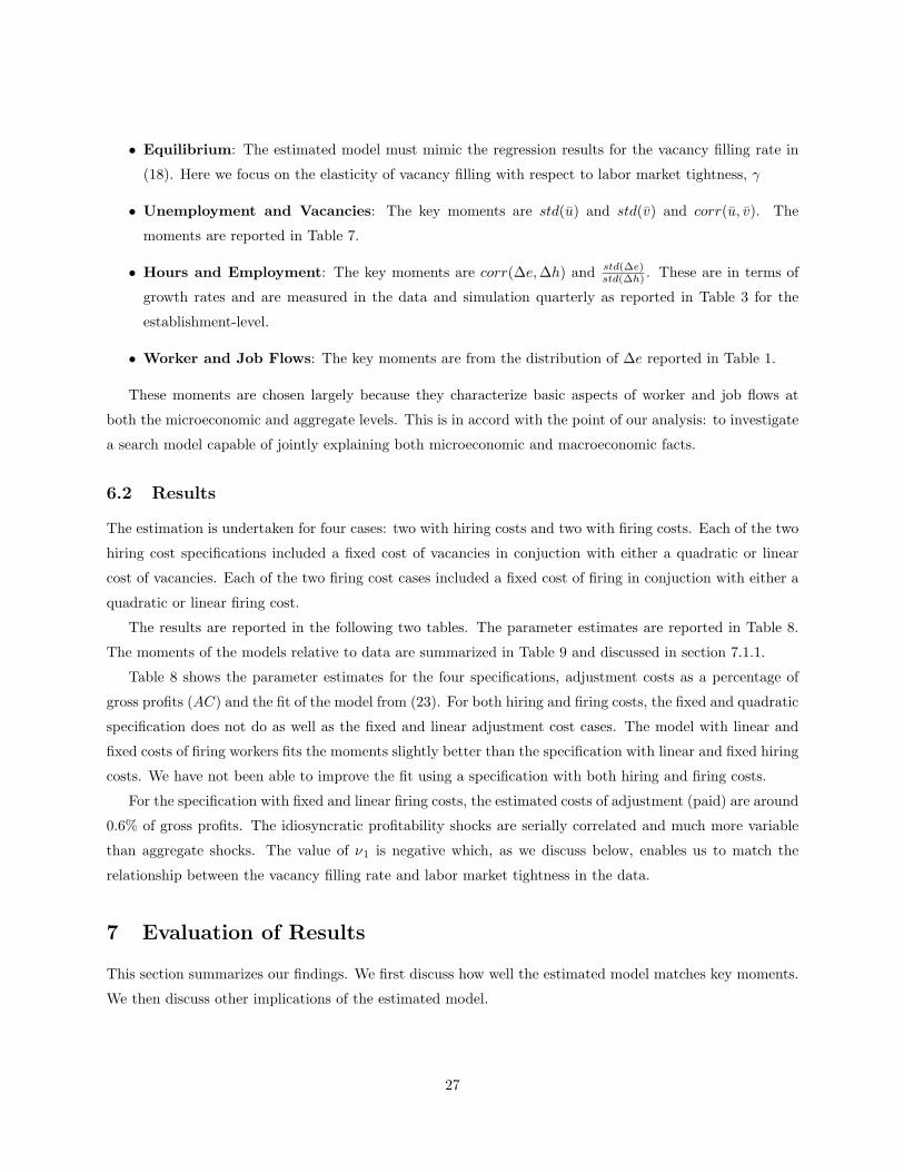
The results are reported in the following two tables. The parameter estimates are reported in Table 8.

The moments of the models relative to data are summarized in Table 9 and discussed in section 7.1.1.

Table 8 shows the parameter estimates for the four specifications, adjustment costs as a percentage of

gross profits (AC) and the fit of the model from (23). For both hiring and firing costs, the fixed and quadratic

specification does not do as well as the fixed and linear adjustment cost cases. The model with linear and

fixed costs of firing workers fits the moments slightly better than the specification with linear and fixed hiring

costs. We have not been able to improve the fit using a specification with both hiring and firing costs.

For the specification with fixed and linear firing costs, the estimated costs of adjustment (paid) are around

0.6% of gross profits. The idiosyncratic profitability shocks are serially correlated and much more variable

than aggregate shocks. The value of ν1 is negative which, as we discuss below, enables us to match the

relationship between the vacancy filling rate and labor market tightness in the data.

7 Evaluation of Results

This section summarizes our findings. We first discuss how well the estimated model matches key moments.

We then discuss other implications of the estimated model.

27

Specification F+ c+0 F− c−0 ν1 ρε σε AC £(Λ)

Hiring Costs

Fixed, Quadratic (c+1 = 2) 0.029 0.004 0 0 -28.05 0.399 0.097 0.6972 0.0806

Fixed, Linear (c+1 = 1) 0.110 0.011 0 0 -39.395 0.312 0.283 0.836 0.0575

Firing Costs

Fixed, Quadratic (c−1 = 2) 0 0 0.107 1.398 -51.731 0.560 0.079 0.0 0.1240

Fixed, Linear (c−1 = 1) 0 0 0.2145 0.062 -46.257 0.479 0.301 0.617 0.0408

Table 8: Estimation Results: Parameters

7.1 Explaining the Moments and Additional Facts

From Table 8, the specification with fixed and linear hiring costs fits the moments best. We call this the

“best fit” specification. Here we discuss how that model matches the moments in more detail and also touch

on other moments.

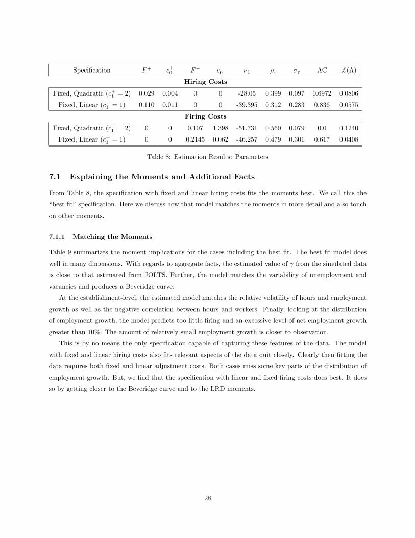
7.1.1 Matching the Moments

Table 9 summarizes the moment implications for the cases including the best fit. The best fit model does

well in many dimensions. With regards to aggregate facts, the estimated value of γ from the simulated data

is close to that estimated from JOLTS. Further, the model matches the variability of unemployment and

vacancies and produces a Beveridge curve.

At the establishment-level, the estimated model matches the relative volatility of hours and employment

growth as well as the negative correlation between hours and workers. Finally, looking at the distribution

of employment growth, the model predicts too little firing and an excessive level of net employment growth

greater than 10%. The amount of relatively small employment growth is closer to observation.

This is by no means the only specification capable of capturing these features of the data. The model

with fixed and linear hiring costs also fits relevant aspects of the data quit closely. Clearly then fitting the

data requires both fixed and linear adjustment costs. Both cases miss some key parts of the distribution of

employment growth. But, we find that the specification with linear and fixed firing costs does best. It does

so by getting closer to the Beveridge curve and to the LRD moments.

28

Mod

elV

aca

ncy

Filling

Unem

plo

ym

ent

and

Vaca

nci

esLR

DJO

LTS:

∆e

γσ(u

)σ(v

)co

rr(u

,v)

σh/σ

eco

rr(h

,e)

<−

0.10

−0.

10<−

0.02

5−

0.02

5<

0.02

50.

025

<0.

10>

0.10

Dat

a0.

354

0.08

60.

116

-0.9

540.

955

-0.2

960.

040

0.08

30.

745

0.09

20.

040

Hir

ing

Cos

ts

Fix

ed,Q

uadr

atic

0.44

40.

041

0.11

9-0

.771

0.96

0-0

.374

0.0

0.0

0.85

20.

027

0.12

1

Fix

ed,Lin

ear

0.40

20.

123

0.14

1-0

.813

0.98

4-0

.414

0.09

70.

089

0.70

50.

00.

109

Fir

ing

Cos

ts

Fix

ed,Q

uadr

atic

0.48

30.

095

0.20

8-0

.695

0.97

2-0

.406

0.0

0.0

0.80

60.

172

0.02

2

Fix

ed,Lin

ear

0.41

30.

125

0.18

03-0

.866

0.99

7-0

.379

0.01

70.

00.

783

0.08

0.12

Tab

le9:

Est

imat

ion

Res

ults

:M

omen

ts

Note

:σ(x

)is

the

standard

dev

iation

ofx.

Unem

plo

ym

entco

mes

from

the

CP

Sand

vaca

nci

esare

dir

ectly

cal-

cula

ted

from

JO

LT

Sat

am

onth

lyfr

equen

cy.

The

vari

able

sare

inlo

gs

and

are

HP

filt

ered

.T

he

emplo

ym

ent

adju

stm

ent

mom

ents

are

size

wei

ghte

dusi

ng

emplo

ym

ent.

29

7.1.2 Other Implications

There are a couple of additional facts, used to motivate this study, which were not included in the set of

moments. One is the regression shown in Table 2. From this regression, establishments expand employment

by hiring and contract through separations. This is not always the case in the models we explored. For

the specification with fixed and quadratic costs of posting vacancies, there was relatively little response of

separation to net employment growth. Due to the adjustment costs, 86% of the observations have zero

vacancies and workers were rarely fired.

For the best fit specification, the regression matches the results in the data very well. The regression

coefficients are very similar to those reported in Table 2.

In terms of inaction, the best fit model did not fit the facts. It predicts too much inaction in vacancies:

there are no vacancies in about 75% of the simulated observations relative to 45% in the data. With the

substantial costs of firing, there is relatively little firing and thus less need to hire workers. When hiring

occurs, there is a burst of job creation.

Both unemployment and vacancies are serially correlated. Those moments were not used in the esti-

mation. In the JOLTS data, the serial correlation of u is 0.92 and of v is 0.91. From simulations of the

estimated model, we find that the serial correlation of unemployment is 0.91 and the serial correlation of

vacancies is 0.70. Thus the model does not quite generate the required serial correlation of vacancies.

7.2 TFP vs. Average Labor Productivity: Unemployment and Vacancies

One of the more interesting points of difference between the empirical literature on aggregate search models

and the macroeconomic literature based on the stochastic growth model is the measurement of productivity.

The search literature largely looks at average labor productivity (ALP) while the macroeconomics literature

focuses on total factor productivity (TFP) as an exogenous shock.

In this paper, we are closer to the tradition of the stochastic growth model. We have treated profitability

as exogenous where the profitability shock summarizes both technological and demand factors influencing the

revenues of a producer. If the model is competitive, then the profitability shock is most naturally interpreted

as a variation in technology.32

For the model we study, revenues are specified in (5). For the one-competitive economy, revenues are the

same as output. If labor is freely mobile (no adjustment costs and no rigidities due to timing assumptions)

between production sites, then the cross sectional distribution of ALP will be degenerate. Further, if the

labor market clears at a constant real wage each period, then the average product of labor will be constant

over time.32Allowing monopolistic competition allows for an interpretation of α as including a markup and the shocks to revenue

including a relative demand disturbance. As the model studied here does not include product differentiation, α and the shocks

should be more narrowly interpreted.

30

Generally though TFP and ALP are not the same. There are two economic forces which together separate

these measures of productivity: (i) frictions in the adjustment process and (ii) idiosyncratic shocks.

To see these influences, think about two extreme economies. In one, suppose that labor flows freely

across producers and in the second suppose there are frictions in labor flows. Suppose the distribution of

idiosyncratic shocks is the same in the two economies and is fixed over time.

As aggregate TFP varies, ALP will vary in both of these economies. For fixed TFP, in the second economy,

ALP will increase as labor flows from less productive to more productive producers. Thus variations in ALP

will generally reflect both TFP and frictions.

Still, ALP is much easier to measure and thus plays a prominent role in the empirical literature. One of

the advantages of our simulation environment is that we can use our model to generate a measure of ALP,

for producer i in period t as

atεi,t(ei,thi,t)α−1. (24)

The value of α used for our analysis is 0.65. In the context of the model, α < 1 reflects the presence

of fixed factors of production such as managerial ability, structures and predetermined components of the

equipment stock.

With these differences between TFP and ALP in mind, we return to a discussion of moments. The puzzle

posed by Shimer (2005) concerned the standard deviation of unemployment and vacancies relative to ALP,

as shown in Table 4. Our estimation, in contrast, has not focused on this moment per se but rather we target

the absolute standard deviations on unemployment and vacancies. The point in doing so was to separate

the inference of ALP from the rest of the model.

Given our estimated model, we simulate average labor productivity and relate it to unemployment and

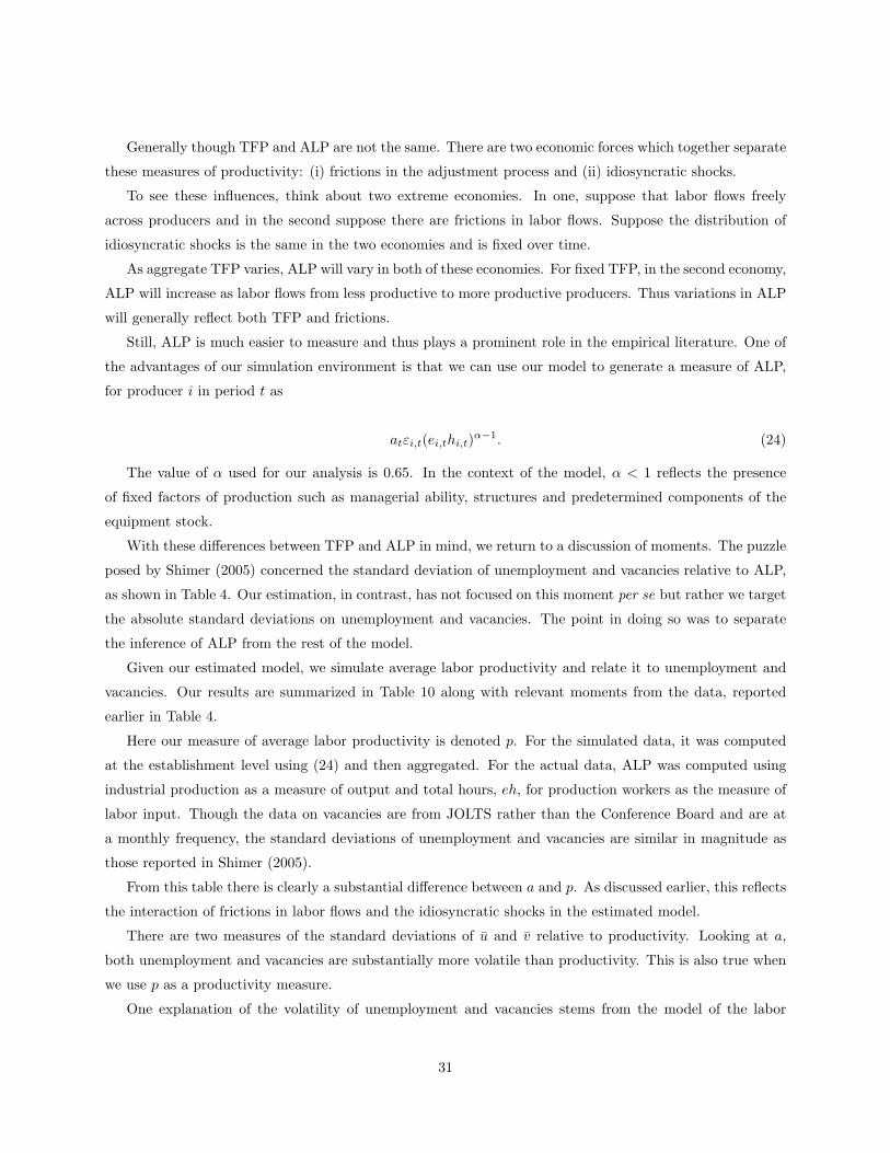
vacancies. Our results are summarized in Table 10 along with relevant moments from the data, reported

earlier in Table 4.

Here our measure of average labor productivity is denoted p. For the simulated data, it was computed

at the establishment level using (24) and then aggregated. For the actual data, ALP was computed using

industrial production as a measure of output and total hours, eh, for production workers as the measure of

labor input. Though the data on vacancies are from JOLTS rather than the Conference Board and are at

a monthly frequency, the standard deviations of unemployment and vacancies are similar in magnitude as

those reported in Shimer (2005).

From this table there is clearly a substantial difference between a and p. As discussed earlier, this reflects

the interaction of frictions in labor flows and the idiosyncratic shocks in the estimated model.

There are two measures of the standard deviations of u and v relative to productivity. Looking at a,

both unemployment and vacancies are substantially more volatile than productivity. This is also true when

we use p as a productivity measure.

One explanation of the volatility of unemployment and vacancies stems from the model of the labor

31

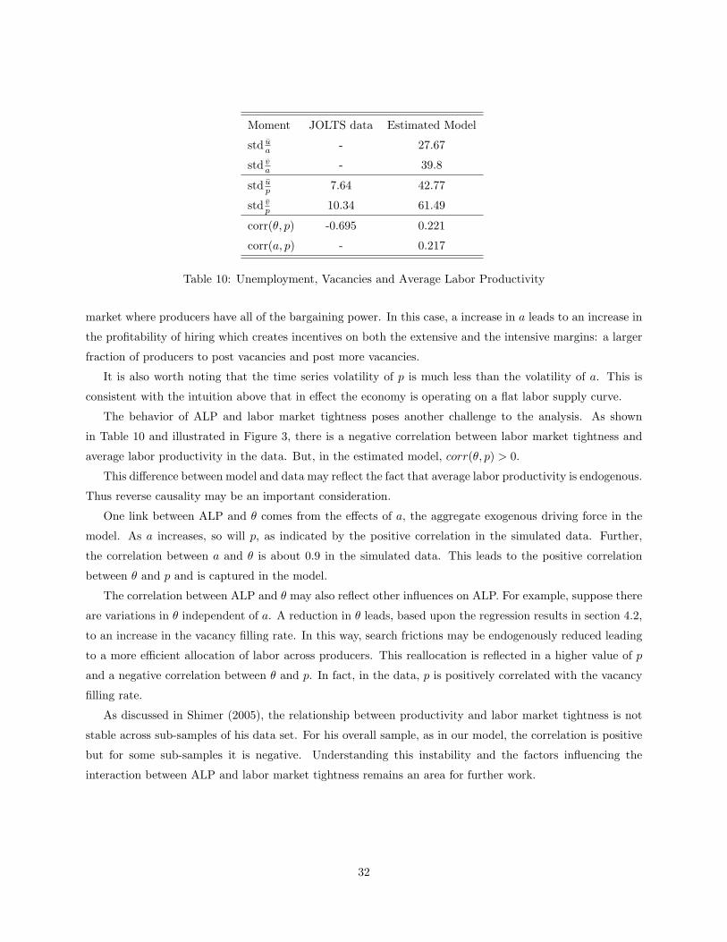
Moment JOLTS data Estimated Model

std ua - 27.67

std va - 39.8

std up 7.64 42.77

std vp 10.34 61.49

corr(θ, p) -0.695 0.221

corr(a, p) - 0.217

Table 10: Unemployment, Vacancies and Average Labor Productivity

market where producers have all of the bargaining power. In this case, a increase in a leads to an increase in

the profitability of hiring which creates incentives on both the extensive and the intensive margins: a larger

fraction of producers to post vacancies and post more vacancies.

It is also worth noting that the time series volatility of p is much less than the volatility of a. This is

consistent with the intuition above that in effect the economy is operating on a flat labor supply curve.

The behavior of ALP and labor market tightness poses another challenge to the analysis. As shown

in Table 10 and illustrated in Figure 3, there is a negative correlation between labor market tightness and

average labor productivity in the data. But, in the estimated model, corr(θ, p) > 0.

This difference between model and data may reflect the fact that average labor productivity is endogenous.

Thus reverse causality may be an important consideration.

One link between ALP and θ comes from the effects of a, the aggregate exogenous driving force in the

model. As a increases, so will p, as indicated by the positive correlation in the simulated data. Further,

the correlation between a and θ is about 0.9 in the simulated data. This leads to the positive correlation

between θ and p and is captured in the model.

The correlation between ALP and θ may also reflect other influences on ALP. For example, suppose there

are variations in θ independent of a. A reduction in θ leads, based upon the regression results in section 4.2,

to an increase in the vacancy filling rate. In this way, search frictions may be endogenously reduced leading

to a more efficient allocation of labor across producers. This reallocation is reflected in a higher value of p

and a negative correlation between θ and p. In fact, in the data, p is positively correlated with the vacancy

filling rate.

As discussed in Shimer (2005), the relationship between productivity and labor market tightness is not

stable across sub-samples of his data set. For his overall sample, as in our model, the correlation is positive

but for some sub-samples it is negative. Understanding this instability and the factors influencing the

interaction between ALP and labor market tightness remains an area for further work.

32

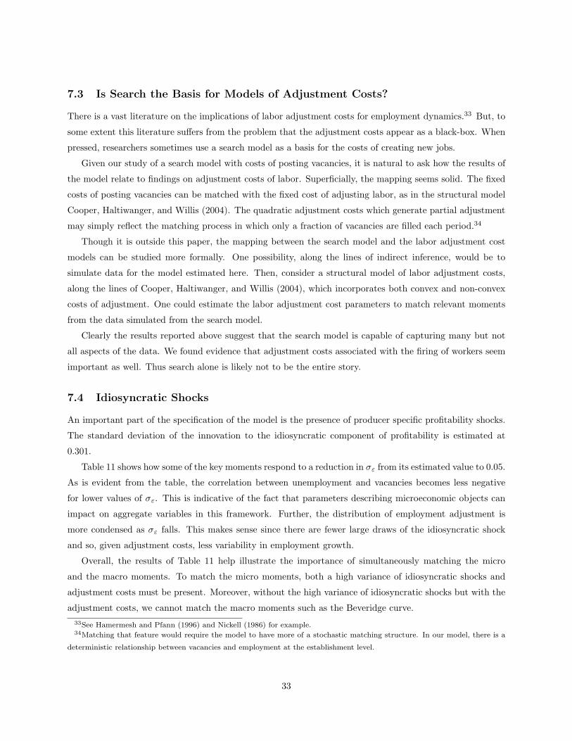
7.3 Is Search the Basis for Models of Adjustment Costs?

There is a vast literature on the implications of labor adjustment costs for employment dynamics.33 But, to

some extent this literature suffers from the problem that the adjustment costs appear as a black-box. When

pressed, researchers sometimes use a search model as a basis for the costs of creating new jobs.

Given our study of a search model with costs of posting vacancies, it is natural to ask how the results of

the model relate to findings on adjustment costs of labor. Superficially, the mapping seems solid. The fixed

costs of posting vacancies can be matched with the fixed cost of adjusting labor, as in the structural model

Cooper, Haltiwanger, and Willis (2004). The quadratic adjustment costs which generate partial adjustment

may simply reflect the matching process in which only a fraction of vacancies are filled each period.34

Though it is outside this paper, the mapping between the search model and the labor adjustment cost

models can be studied more formally. One possibility, along the lines of indirect inference, would be to

simulate data for the model estimated here. Then, consider a structural model of labor adjustment costs,

along the lines of Cooper, Haltiwanger, and Willis (2004), which incorporates both convex and non-convex

costs of adjustment. One could estimate the labor adjustment cost parameters to match relevant moments

from the data simulated from the search model.

Clearly the results reported above suggest that the search model is capable of capturing many but not

all aspects of the data. We found evidence that adjustment costs associated with the firing of workers seem

important as well. Thus search alone is likely not to be the entire story.

7.4 Idiosyncratic Shocks

An important part of the specification of the model is the presence of producer specific profitability shocks.

The standard deviation of the innovation to the idiosyncratic component of profitability is estimated at

0.301.

Table 11 shows how some of the key moments respond to a reduction in σε from its estimated value to 0.05.

As is evident from the table, the correlation between unemployment and vacancies becomes less negative

for lower values of σε. This is indicative of the fact that parameters describing microeconomic objects can

impact on aggregate variables in this framework. Further, the distribution of employment adjustment is

more condensed as σε falls. This makes sense since there are fewer large draws of the idiosyncratic shock

and so, given adjustment costs, less variability in employment growth.

Overall, the results of Table 11 help illustrate the importance of simultaneously matching the micro

and the macro moments. To match the micro moments, both a high variance of idiosyncratic shocks and

adjustment costs must be present. Moreover, without the high variance of idiosyncratic shocks but with the

adjustment costs, we cannot match the macro moments such as the Beveridge curve.33See Hamermesh and Pfann (1996) and Nickell (1986) for example.34Matching that feature would require the model to have more of a stochastic matching structure. In our model, there is a

deterministic relationship between vacancies and employment at the establishment level.

33

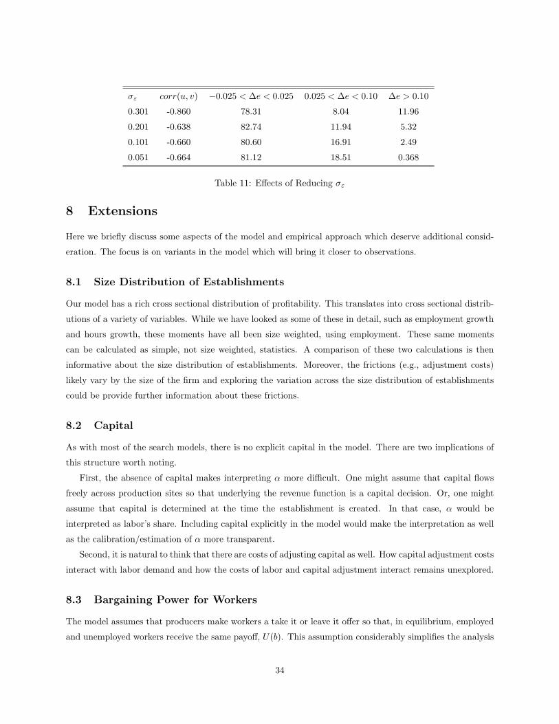
σε corr(u, v) −0.025 < ∆e < 0.025 0.025 < ∆e < 0.10 ∆e > 0.10

0.301 -0.860 78.31 8.04 11.96

0.201 -0.638 82.74 11.94 5.32

0.101 -0.660 80.60 16.91 2.49

0.051 -0.664 81.12 18.51 0.368

Table 11: Effects of Reducing σε

8 Extensions

Here we briefly discuss some aspects of the model and empirical approach which deserve additional consid-

eration. The focus is on variants in the model which will bring it closer to observations.

8.1 Size Distribution of Establishments

Our model has a rich cross sectional distribution of profitability. This translates into cross sectional distrib-

utions of a variety of variables. While we have looked as some of these in detail, such as employment growth

and hours growth, these moments have all been size weighted, using employment. These same moments

can be calculated as simple, not size weighted, statistics. A comparison of these two calculations is then

informative about the size distribution of establishments. Moreover, the frictions (e.g., adjustment costs)

likely vary by the size of the firm and exploring the variation across the size distribution of establishments

could be provide further information about these frictions.

8.2 Capital

As with most of the search models, there is no explicit capital in the model. There are two implications of

this structure worth noting.

First, the absence of capital makes interpreting α more difficult. One might assume that capital flows

freely across production sites so that underlying the revenue function is a capital decision. Or, one might

assume that capital is determined at the time the establishment is created. In that case, α would be

interpreted as labor’s share. Including capital explicitly in the model would make the interpretation as well

as the calibration/estimation of α more transparent.

Second, it is natural to think that there are costs of adjusting capital as well. How capital adjustment costs

interact with labor demand and how the costs of labor and capital adjustment interact remains unexplored.

8.3 Bargaining Power for Workers

The model assumes that producers make workers a take it or leave it offer so that, in equilibrium, employed

and unemployed workers receive the same payoff, U(b). This assumption considerably simplifies the analysis

34

since workers need not consider the distribution of employment opportunities in the economy. To do so

would require the state space for workers decisions to include the cross sectional distribution of establishment

profitability shocks. In addition, solving for an equilibrium would require the determination of the market

clearing equilibrium level of expected utility on a state-by-state basis.

Clearly there are gains to tractability through these assumptions. But, the model does imply that

unemployed and employed workers have the same levels of expected utility. Thus could occur even if workers

have bargaining power but would as long as state contingent severance pay was feasible. Otherwise, the

bargaining power of workers could create a gap in utility between employed and unemployed workers. This

is a common property of search models.

As discussed in Hagedorn and Manovskii (2006), both the bargaining weight and thus the utility of

unemployed relative to employed workers impact the cyclical properties of the model. Thus understanding

the quantitative implications of relaxing the assumptions made on the bargaining process would be a useful

extension of this framework. Among other things, this would imply that the cross sectional distribution of

productivity would be part of the state vector and thus another source for richer dynamics.

8.4 Quits

The model we study allows for quits which are deterministic at the establishment-level. In fact, we have

imposed a constant quit rate at each establishment since the model does not have a rich theory of quits given

the result that V e = V u. In reality, quits are stochastic and endogenous.

For small establishments, the randomness in quits is not nullified by the law of large numbers. Thus, on

a monthly basis, the quit rate ought to be modeled as stochastic rather than deterministic.

Further, Table 1 makes clear that quits are not independent of the employment growth at the establish-

ment. When employment growth is negative, the quit rate is apparently higher.

Extending the model to include stochastic and endogenous quits may be important for matching obser-

vations on the frequency of zero net employment growth, about 30% of observations, and the frequency of

zero vacancies, about 45% of observations. With deterministic quits and non-convex adjustment costs, it

is not possible to explain inaction in both vacancies and net employment growth. Still, it is not clear how

much impact a richer model of quits would have on the aggregate implications of the model.

9 Conclusions

The goal of this paper was to study the implications of a search model for observed movements in:

• unemployment and vacancies at the aggregate level,

• employment and hours variations at the establishment level,

• the distribution of net employment growth at the establishment level.

35

While each of these aspects of the data have been explored independently in other studies, it is valuable

to look jointly at these observations. The micro evidence guides and disciplines the models built to match

aggregate observations and the models based on the establishment level ought to be challenged to match

aggregates.

Our framework is an extension of the standard search model with two features. First, in order to match

establishment level observations, we introduce non-convexities into the process of posting vacancies along

with convex adjustment costs. Second, we introduce hours variations into the search model through an

ex ante labor contracting structure. Both of these features require us to create a nontrivial model of the

producer. Finally, as in Mortensen and Pissarides (1994), establishment specific shocks play a prominent

role in the analysis and in the moments generated by the model.

The returns on these novel modeling features accrue from insights into the costs of vacancies and firing

and the ability of the model to resolve some of the puzzling aspects of the data. In that regard, we find:

• fixed and linear adjustment costs are necessary to match observations,

• the model with firing costs is slightly closer to the data than is the model with vacancy costs

• the model is able to match observed co-movements in hours and employment growth at the establish-

ment level.

• the model does not suffer from the amplification problem highlighted in Shimer (2005)

• the model does match some of the inaction and bursts reported for vacancies and employment adjust-

ment at the establishment level.

The paper concludes with a list of extensions to consider. These are intended to further shrink the gap

between the model and facts about labor markets.

36

References

Azariadis, C. (1975): “Implicit Contracts and Underemployment Equilibria,” Journal of Political Economy,

83(6), 1183–1202.

Cole, H., and R. Rogerson (1996): “Can the Mortensen-Pissarides Matching Model Match Business

Cycle Facts?,” Federal Reserve Bank of Minneapolis, Staff Report #224.

Cooper, R., J. Haltiwanger, and J. Willis (2004): “Dynamics of Labor Demand: Evidence From

Plant-Level Observations and Aggregate Implications,” NBER Working Paper #10297.

Davis, S., R. Faberman, and J. Haltiwanger (2006a): “The Flow Approach To Labor Markets: New

Data Sources And Micro-Macro Links,” NBER Working Paper #12167.

(2006b): “The Micro-Level Behavior of Vacancies and Hiring,” mimeo.

Faberman, R. J. (2005): “Analyzing the JOLTS Hires and Separations Data,” Proceedings of the 2005

American Statistical Association.

Fujita, S., and G. Ramey (2005): “The Dynamic Beveridge Curve,” http://www.phil.frb.org/files/

wps/2005/WP05-22.pdf, Federal Reserve Bank of Philadelphia, Working Paper #05-22.

Hagedorn, M., and I. Manovskii (2006): “The cyclical behavior of equilibrium unem- ployment and

vacancies revisited,” http://www.econ.upenn.edu/~manovski/papers/BCUV.pdf, Mimeo, University of

Frankfurt and University of Pennsylvania.

Hall, R. (2005): “Employment Fluctuations with Equilibrium Wage Stickiness,” American Economic Re-

view, 95, 53–69.

Hamermesh, D., and G. Pfann (1996): “Adjustment Costs in Factor Demand,” Journal of Economic

Literature, 34, 1264–92.

Mortensen, D. T., and C. A. Pissarides (1994): “Job Creation and Job Destruction in the Theory of

Unemployment,” Review of Economic Studies, 61, 397–415.

Nickell, S. (1986): “Dynamic Models of Labor Demand,” in Handbook of Labor Economics, ed. by

O. Ashenfelter, and R. Layard. Amsterdam: North Holland.

Shimer, R. (2005): “The Cyclical Behavior of Equilibrium Unemployment and Vacancies,” American Eco-

nomic Review, 95, 25–49.

Tasci, M. (2006): “On the Job Search and Labor Reallocation,” http://www.eco.utexas.edu/graduate/

Tasci/ojsandlmr.pdf.

37

Willis, J. (2003): “General Equilibrium of a Monetary Model with State Dependent Pricing,” http:

//www.kc.frb.org/Econres/addfiles/sdp_jlw.pdf.

Yashiv, E. (2000): “The Determinants of Equilibrium Unemployment,” American Economic Review, 90,

1297–1322.

(2006): “Evaluating the Performance of the Search and Matching Model,” European Economic

Review.

38

..

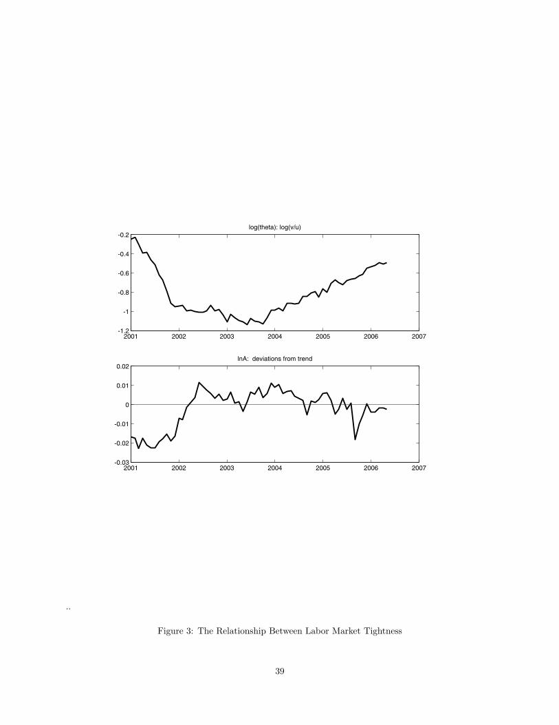
2001 2002 2003 2004 2005 2006 2007-1.2

-1

-0.8

-0.6

-0.4

-0.2log(theta): log(v/u)

2001 2002 2003 2004 2005 2006 2007-0.03

-0.02

-0.01

0

0.01

0.02lnA: deviations from trend

Figure 3: The Relationship Between Labor Market Tightness

39