Hotelling's Rule in the limit: an

agent-based exploration of the model

space

David S. Dixon∗

April 23, 2012

Hotelling's Rule is the observation that the exploitation of a nonrenewableresource can only be economically e�cient if the resource owner's marginalpro�t increases at the prevailing discount rate. This has been a perennial topicin the literature of resource economics since the 1970s, with some authors ex-tending the theory and others analyzing empirical data. This paper reports onthe results from using agent-based modeling to assess the consequences of re-laxing the optimality constraint to explore the ways in which the outcome spaceconverges on Hotelling's Rule in the limit. The agent-based model (ABM) inthis paper has one choice variable: increase, decrease, or maintain the currentproduction level - based on one rule: choose the change in production levelthat maximizes estimated discounted pro�t. The results, based on a costlesstechnology and a stylized demand function from Hotelling, indicate that to-tal discounted pro�t has low sensitivity to deviations from the optimum. Inextending the basic Hotelling model to stylized production technologies withcost, the simple ABM falls short of the optimum by as much as ten percent,depending on the magnitude and whether the cost is �xed, marginal, or basedon the resource stock level. The optimization errors of the ABM are similar tothe errors of a human production planner with incomplete information. TheABM also exhibits emergent collusion-like and Cournot-like behaviors whenextended to a small oligopoly market.(JEL Q32)

∗Department of Economics, MSC 05 3060, 1 University of New Mexico, Albuquerque, NM 87131-0001,ddixon@unm.edu. The author acknowledges the invaluable guidance and assistance of Janie Chermak,the comments and suggestions of Robert Solow, Gérard Gaudet and Meghan Hutchins, and the technicalassistance of Denise Stark of Aptech. The MASON and GAUSS code for these models is available fromhttp://www.unm.edu/~ddixon.

1

Keywords: Hotelling's Rule; agent-based modeling; agent-based computationeconomics.

�They're more what you'd call guidelines than actual rules.�

-Hector Barbosa in Pirates of the Caribbean:

The Curse of the Black Pearl

With regard to Hotelling's Rule, Captain Barbosa might well have said �it's more whatyou'd call an outcome than an actual rule.� Hotelling (1931) observes that the owner ofa �nite natural resource is indi�erent to either exploiting it or leaving it in situ when themarginal pro�t increases at the prevailing interest rate. The rationale is that, if the returnis lower than this, the resource owner will shift assets to a better performing investment.If the return is greater, the owner will leave the resource where it is as it appreciates fasterthan other investments. In other words, the resource will not be produced at all unless itcan be produced at a rate that returns the prevailing interest rate.Hotelling noted that this sets the upper limit on a monopoly producer's pro�t from pro-

duction. To explain this, it is necessary to appeal to the law of demand. For a downward-sloping demand curve, the monopoly producer can only increase the price by decreasing theproduction level. Hotelling's Rule says that if the producer decreases production at a ratethat makes the marginal pro�t change by the interest rate, total pro�t from the resourcewill be maximized. If the production level is changed in any other way, total pro�t will beless than the maximum.Hotelling's Rule is often called the r-percent rule and paraphrased as �the price must

increase by r percent,� r referring to the interest rate.1 The producer pro�t, or scarcityrent, is paid by the consumer, and is also called user cost. If pro�t is increasing by r-percent,then user cost is also increasing by r-percent. Using dynamic optimization, Hotelling showsthat the r-percent rule is the outcome of the producer maximizing pro�t, rather than arule for the producer to follow.The responsibility for naming it a rule may fall on Robert Solow, who �rst used the term

�Hotelling's rule� in his Ely Lecture presented to the 1973 conference of the American Eco-nomic Association (Solow, 1974, p 12). In reference to this, Solow re�ects that �Hotelling'sconcept is not a 'rule' at all in the appropriate sense. It doesn't enjoin anything. Phelps'sGolden Rule is and does. Hotelling's principle is a description of what a foresighted com-petitive market would do, under simple conditions. Neither Phelps's nor Hartwick's rulehas that property. They have to be imposed.�2 Nonetheless, the term �Hotelling's Rule�appears in countless texts and papers and is well-known - even beloved - to generations ofnatural resource economists.

1Strictly speaking, price is not identical to marginal pro�t, particularly in a monopoly market.2From a personal communication dated 25 May 2010.

2

1 Background

Gaudet (2007) presents an excellent historical and contextual background for Hotelling's1931 paper, from which the points in this paragraph are excerpted. The potential exhaus-tion of natural resources was a politically charged topic in the early twentieth century. Earlyeconomic models of exhaustible natural resources were based on static equilibrium, moti-vating Hotelling to develop a dynamical model. The result was a �rst-order optimization,with reference to speci�c cases requiring calculus of variations. Though straightforward bymodern standards, the approach was mathematically sophisticated for the time, so the key�nding languished until interest in exhaustible resources reemerged in the 1970s.Devarajan and Fisher (1981) review the �rst �fty years of theoretical developments based

on the Hotelling model. Much of that work is shown to pertain to issues that Hotellingraised but did not pursue, such as the e�ects of cumulative production and uncertainty instock size. Krautkraemer (1998) adds another decade and a half and includes developmentsin the econometric search for evidence of Hotelling's Rule. Another ten years are added tothe Hotelling time line by Livernois (2009). For the purposes of this paper, there are twomain themes of interest in the Hotelling's Rule literature: theoretical e�orts to broadenthe scope of Hotelling's Rule, and econometric e�orts to �nd evidence of the Hotelling'sRule outcome.

1.1 The evolving theory of nonrenewable resources

Hotelling's Rule says that scarcity rents must be increasing by r-percent, which implies,ceteras paribus, that price should be increasing by r-percent. There are, however, theoret-ical bases for decoupling the trend in market price from the trend in scarcity rents. Solow(1974, p. 3) suggests that if extraction costs fall by more than scarcity rents increase,the trend in market price may be downward. He notes, however, that eventually scarcityrent will dominate market price. Krautkraemer (1998) presents theoretical extensions tothe Hotelling model to take into account variable stock levels due to exploration, cost ofcapital, capacity constraints, ore quality, and market imperfections.Heal (1976) presents a model in which stock e�ects produce a declining resource value.

Levhari and Liviatan (1977) explore the conditions under which a resource becomes eco-nomically nonviable but not physically depleted, a situation that arises with cumulativeproduction (stock) costs. Livernois and Martin (2001) illustrate circumstances in whichmarket prices rise while scarcity rents decline to zero because of resource degradation.Pindyck (1978) and Livernois and Uhler (1987) suggest that bringing new deposits into

production as the result of exploration produces a U-shaped price path. Slade (1982)proposes a U-shaped price trend due to technological advances early in production andscarcity rents late in production. Similarly, Dasgupta and Heal (1980) and Arrow andChang (1982) propose models of exploration that produce a saw-tooth price curve. Cairnsand Van Quyen (1998) propose a model that combines exploration and stock e�ects inwhich the price trend is downward for most of the stock lifetime, but rises to the choke

3

price at the end.Much of the preceding theoretical development is motivated by studies of various re-

source markets in which no long-term price increase is evidenced. Each represents a majorundertaking to explore a simple extension of the Hotelling model, with the exception ofCairns and Van Quyen (1998), which incorporates two simple extensions.Hotelling presents a perfectly competitive model and a monopoly model, then makes

suggestions as to what happens when it is a duopoly market. He describes what, in gametheory parlance, is called the cooperation-defection problem. Hotelling notes that withan exhaustible resource, the defector has an incentive to raise the price, unlike in staticequilibrium in which the defector has cause to lower price (and increase sales). With anexhaustible resource, the defector knows that if the competitor doesn't match the higherprice, the defector will be at an advantage later as the resource becomes more scarce.Salant (1976) presents a highly notional model of prices in an oligopoly market for an

exhaustible resource. An intriguing outcome of this model is that, for a market where somecompetitors form a cartel and the rest do not, a portion of the scarcity rents is transferredaway from the cartel to be shared by the competitive fringe.Stiglitz (1976) observes that a monopoly in an exhaustible resource market has less

market power than in the market for a non-exhaustible resource. This point is supportedby Lewis et al. (1979) and con�rmed by Pindyck (1987). The result is challenged byGaudet and Lasserre (1988), however, who point out the Stiglitz non-exhaustible modelassumes in�nite input capacity, while inputs in the exhaustible models are, by de�nition,limited. By treating the monopoly and competitive models as having the same inputcapacity constraint, Gaudet and Lasserre show that the monopolist's market power is thesame whether the resource is exhaustible or not.The principal barrier to theoretical expansion of the Hotelling model is that dynamic

optimization is di�cult to characterize in general terms. Hotelling found it necessary toresort to speci�c demand functions in order to explore implications of the base, costlessmodel. (Livernois, 2009) notes that the Hotelling model becomes complex when extendedto include factors like resource degradation. Krautkraemer (1998) is able to make generalstatements about the stock cost term by breaking the base case into a bene�t term and acost term, but does not carry the theoretical development into the extensions.Agent-based modeling can be a laboratory for exploring and experimenting with pro-

posed extensions to the Hotelling model. Because agent-based modeling is a causal frame-work, the researcher must express the behavior in terms of what an agent - a resourceproducer, for example - would do under conditions that arise in simulation. For an explo-ration model in which the resource deposits are discovered in decreasing quality (Pindyck,1987, Livernois and Uhler, 1987), the new deposits come into existence sequentially: eachdeposit is exploited until its costs equal those of the next most costly (lesser quality) de-posit, then production shifts to that one. In other models the quality of newly discovereddeposits is random (Swierzbinski and Mendelsohn, 1989), which has the e�ect of �atteningthe price curve. Agent-based modeling is well suited to comparing the outcomes of thesetwo models.

4

1.2 Studies of the markets for nonrenewable resources

A decade before the birth of modern environmental and natural resource economics in the1970s, Barnett and Morse (1963) �nds that, over the period 1870 to 1957, resource pricesshow no discernible trend, despite continuous and often rapid increases in their production.More then a decade and a half later, Smith (1979) con�rms these �ndings using moresophisticated techniques on data from 1900 to 1973. Fisher (1981, p. 102-103) concursthat there are no discernible trends in overall resource prices in the results of Barnett andMorse (1963), but notes that factor costs fell more rapidly than resource prices during thisperiod, so there is evidence for some increase in rents during that time. Alternatively,Brown and Field (1978) assert that Barnett and Morse neglected to include some factorcosts, notably transportation. Brown and Field point out that the �rst three-quarters ofthe twentieth century - the period covered by the study - was a period of dramatic technicaland social change.Halvorsen and Smith (1991) note that �the principle obstacle to empirical tests of the

theory of exhaustible resources has been data availability.� Since actual marginal cost and,therefore, actual user cost, are not observable, many of the market studies are essentiallyassessments of the suitability of proxies for these.Nordhaus (1973, p. 566) observes that, on the average, scarcity rents on energy resources

were "quite modest," on the order of one dollar per barrel of petroleum.3 He notes thatthe exception was petroleum itself, for which market prices were 2.4 times his calculatedoptimal price, which includes scarcity rent. A year later, Nordhaus (1974) found no trendin mineral prices between 1900 and 1970. Nordhaus is responsible for the term "backstoptechnology," referring to nuclear power as the technology that would, ultimately, limit themaximum price on petroleum and eliminate energy scarcity (Nordhaus, 1973, p. 532).Some researchers have found evidence of U-shaped price curves, such as Slade (1982),

who postulated that the price trend was due to falling input costs early in production andrising scarcity costs at the end of resource lifetime. Berck and Roberts (1996) examinea larger data set that includes most of the data used by Slade. They �nd that pricepredictions depend on whether prices are modeled as trend-stationary or as di�erence-stationary. They also �nd that trend-stationary models predict rising resource prices whiledi�erence-stationary models are ambiguous.Heal and Barrow (1980) develop an arbitrage model which is an attempt to detect,

directly, the Hotelling outcome. They assert that, in an e�cient resource market, �therewill be a strong association between the rates of change of resource prices and the ratesof return on other assets.� They found, however, that changes in interest rates were therelevant explanatory variables, not the interest rate levels. They conclude that simpleequilibrium theory is inadequate to the complexity of the problem.Stollery (1983) estimates the cost function for the price-leader in the nickel market and

infers user cost by subtracting marginal cost from market price. User cost is found to be

3For the years 1970-1973, crude oil prices averaged less than three dollars per barrel in current dollars.http://www.eia.doe.gov/aer/txt/ptb1107.html (accessed 14 April 2011)

5

low initially, but to increase by 15 percent. Farrow (1985), using proprietary mine data,presents a model to estimate the in situ value of the stock and compares that with theprice trend. He does not �nd evidence of Hotelling's Rule.Halvorsen and Smith (1984) introduce duality to estimate in situ stock value for Cana-

dian metal mines and �nd that user cost decreased considerably. Chermak and Patrick(2001) also appeal to duality to estimate in situ stock value and �nd that, for 29 naturalgas wells, the trend is consistent with Hotelling's Rule.(Agostini, 2006) found no evidence of U.S. copper companies exercising oligopoly market

power before 1978, when U.S. copper went on the world market. He suggests a possibleexplanation is that the copper �rms did exercise market power for brief periods, but limitedprices during periods of high demand as a barrier to new entrants.The preceding studies are a sample of the variety of markets and methodologies applied

to this problem, and the results are often intriguing, but seldom conclusive. �However, theability of the theory of exhaustible resources to describe and predict the actual behaviorof resource markets remains an open question.�(Halvorsen and Smith, 1991)

1.3 Agent-based computational economics

In the social sciences, one early adopter of agent-based modeling is Robert Axelrod (1997),whose models started out as an extension of earlier work on the Prisoner's Dilemma in gametheory (1987). Agent-based modeling �ourished as computation became faster, cheaper,and widely available. Many of the behavioral models developed theoretically in the pre-ceding decades, such as Axelrod's and those of Thomas Schelling (1978) were well suitedto agent-based modeling. Epstein and Axtell, both jointly and separately, develop agent-based models including an adaptation of a cultural transmission model by Axelrod (Axtellet al., 1996), the emergence of classes (Axtell et al., 1999) and civil violence (Epstein, 2002).McFadzean et al. (2001) introduce agent-based modeling as a computational laboratory fortrade networks, and Tesfatsion (2001) applies the approach to an adaptive search modelof the labor market. The dynamic and emergent behaviors of agents in combat are exam-ined in Reynolds and Dixon (2001) and Dixon and Reynolds (2003), while the latter alsomodels how a national bond market crisis spreads globally. Gilbert and Troitzsch (2005)provide an overview of various topics in modeling and simulation of social systems, includ-ing agent-based modeling. Tesfatsion (2006) provides examples of agent-based models thatcorrespond to and often extend traditional economic models.A note about the initials ABM. They are used to refer to the methodology of agent-based

modeling, or to an agent-based model. That is �we will use ABM to explore Hotelling'sRule by constructing multiple ABMs, each representing a di�erent cost structure.� Inthis paper, agent-based modeling is referenced in its entirety, while the initials ABM arereserved for the models.Although many ABMs are ad hoc computer programs, groups within the agent-based

community have developed programs to automate the modeling and simulation process tosome extent. MASON, a project at George Mason University, is an example, and is used

6

for the modeling and simulation presented in the following chapters. For more details onMASON, see the website.4 The MASON code for this paper is available for download.5

2 Theory

"Problems of exhaustible assets cannot avoid the calculus of variations" noted Hotelling(1931, p. 140), which may have been why his work languished until the 1970s (Gaudet,2007, p. 1035). Since its advent, optimal control theory (Pontryagin, 1959, Pontryaginet al., 1962) has become a standard tool for dynamic optimization in economics. Chiang(1992) notes that, unlike calculus of variations, optimal control can be used with functionsthat are piecewise continuous or that have corner solutions. The introductory optimalcontrol problem in Chiang (1992) is the Hotelling model. Caputo (2005) observes thatoptimal control theory is more conducive to economic theory and intuition than calculusof variations.The following is an optimal control development of the Hotelling monopoly model. The

terminology and some notation derive from Kamien and Schwartz (1981), in particular, theuse of m(t) as the current value multiplier. The notation for partial derivatives is borrowedfrom Caputo (2005), and the economic interpretations are in�uenced by Krautkraemer(1998).The Hotelling monopoly model begins with a known �xed stock x0 of a nonrenewable

resource. The problem for the resource owner is to determine a production path q(t) thatmaximizes present value total net pro�t over the productive lifetime, T , of the resource. Ingeneral, net pro�t π (q (t) , x (t) , t) is a function of production level, remaining stock levelx(t) and time. Assuming a constant discount rate r, the optimal control problem is

maxqJ (q (t) , x (t)) =

ˆ T

0

e−rtπ (q (t) , x (t) , t) dt (1)

subject to these constraints

x (t) = −q (t)

x (0) = x0

x (t) ≥ 0 (2)

q (t) ≥ 0 (3)

x0 ≥T

0

q (t) dt (4)

4http://www.cs.gmu.edu/~eclab/projects/mason/ (accessed 25 June 2010)5http://www.unm.edu/~ddixon (accessed 28 June 2010)

7

The �rst constraint is also the state equation and will be discussed subsequently. Thenext two constraints are the initial and terminal boundary conditions on the stock variable.The fourth constraint ensures that production is never negative, and the �fth ensures thattotal production never exceeds total resource stock.The current-value Hamiltonian to maximize (1) with resource stock costate variablem(t)

is de�ned as

H (q (t) , x (t) , t,m) ≡ π (q (t) , x (t) , t)−m (t) q (t) (5)

The current-value formulation has the advantage that, since the ABM will be makingdecisions based on current state values, a direct comparison can be made between thestate of the ABM at time t and the optimal state of the Hamiltonian at time t. Thecostate variable m(t) is interpreted as the current-value shadow price of the resource stockat time t. This is the user cost of the next unit of remaining stock to be extracted.The �rst order necessary conditions include the state equation

x (t) = −q (t) (6)

which imposes the dynamical constraint that the remaining stock be reduced at the rateof production, where x (t) is the time derivative of x (t). The �rst order necessary costateequation is

m (t) = rm (t)− ∂H (q (t) , x (t) , t,m)

∂x (t)(7)

where m (t) is the time derivative of m (t). If the Hamiltonian has no stock e�ect (nox (t) dependency), this equation requires that the shadow price increase at the rate of thediscounted shadow price, thus ending at some maximum value. Depending on its sign,the stock e�ect may accelerate or decelerate the increase in the shadow price, or, for asu�ciently positive stock e�ect, cause the shadow price to decrease over time.The �rst order necessary optimality condition is

∂H (q (t) , x (t) , t,m)

∂q (t)= 0 (8)

which is the condition for static optimum, requiring that the Hamiltonian be maximizedat all times. The transversality condition on the state variable is that

e−rTm (T ) = 0, x (T ) = 0, e−rTm (T )x (T ) = 0 (9)

8

which constrains the ending shadow price to be non-negative and the ending stock levelto be non-negative, but requires that the shadow value (m× x) of the ending stock mustbe zero. That is, either the stock is physically depleted and x (T ) = 0, or the presentvalue ending shadow price e−rTm (T ) is zero. The latter condition can arise irrespective ofthe ending shadow price if the terminal time T can be in�nite. For nonzero ending stockand �nite T , that the shadow price goes to zero is intuitive, since terminating while thereis remaining stock implies that it is not economic to extract the next unit of stock. Ifthe stock variable is constrained to end at some value, the transversality condition on theHamiltonian is that

e−rTH (T ) = 0 (10)

This ensures that the stock variable is stationary at the terminal time T (Chiang, 1992, p.182).The following relations are introduced for notational simplicity

πq (q (t) , x (t) , t) =∂

∂qπ (q (t) , x (t) , t)

πx (q (t) , x (t) , t) =∂

∂xπ (q (t) , x (t) , t)

Hq (q (T ) , x (T ) , T,m) =∂H (q (t) , x (t) , t,m)

∂q

∣∣∣∣t=T

Substituting for the Hamiltonian in (7)

m (t) = rm (t)− πx (q (t) , x (t) , t) (11)

so that πx (q (t) , x (t) , t) is the Hamiltonian stock a�ect to which the previous remarks ap-ply. That is, the rate at which the shadow price changes is either accelerated or deceleratedby the πx (q (t) , x (t) , t) depending on its sign and, if πx (q (t) , x (t) , t) = 0, shadow priceincreases at the discount rate.Substituting for the Hamiltonian in (8)

πq (q (t) , x (t) , t)−m (t) = 0

πq (q (t) , x (t) , t) = m (t) (12)

which establishes the link between marginal pro�t and shadow price. Substituting (12)into (11) to eliminate m (t), then dividing by πq (q (t) , x (t) , t)

πq (q (t) , x (t) , t)

πq (q (t) , x (t) , t)= r − πx (q (t) , x (t) , t)

πq (q (t) , x (t) , t)(13)

9

which is the general expression of Hotelling's Rule. For a production technology that hasno dependence on the stock level, this simpli�es to

πq (q (t) , x (t) , t)

πq (q (t) , x (t) , t)= r (14)

which is the relation �rst articulated by Hotelling. It states that, on the optimal productionpath, the percent change in marginal net pro�t is equal to the discount rate.

2.1 The Hotelling monopoly demand function

Hotelling's inverse demand function for the monopoly market Hotelling (1931, sec. 4) is

p =(1− e−Kq

)/q (15)

This is a stylized demand not linked to any real market. It is not known why Hotellingchose it, but it has two pedagogical strengths. First, it yields tractable expressions forrevenue and marginal pro�t and secondly, it has no �nite static maximum with respect toq. That is, it can only be maximized in the dynamic context. Additionally, pro�t increasesmonotonically with q, a characteristic that is exploited in the models for which pro�t mustbe held above cost.Equation (15) is the inverse demand function used throughout this paper, in the the-

oretical development and in the agent-based models. For Hotelling's costless productiontechnology, the optimal production path is easily solved in closed form. However, for thenonzero-cost technologies, it is necessary to appeal to numerical solutions. In those cases,and in the agent-based models, the parameter values used are

K = 5

r = (1 + 0.1)1/365.25 − 1 ≈ 2.16× 10−4

x0 = 100

These are all stylized and unitless values. K is the choke price and this value is chosen tobe consistent with the other models used by Hotelling. The discount rate is ten percentper annum and is expressed in daily terms for use in and comparison with the agent-basedmodels. The initial stock x0 is chosen so that simulations of the agent-based models arelong enough to be instructive yet short enough to be repeated many times.

2.2 A costless monopoly model

Costless production technology means that there is no cost term, so that pro�t is equal torevenue

10

π (q (t)) = p (q (t)) q (t) (16)

An optimizing costless monopoly producer, facing the full demand function, determinesthe optimal production path q (t) based on the discount rate r, the extent of stock x0, andany other boundary conditions. For the costless model, the stock is physically depleted attime T . Given a speci�c inverse demand function, the procedure is:

1. Solve (12) for the production path q (t) in terms of m(t).

2. Solve (11) to get m(t).

3. Replace m(t) in q(t) and solve (10) to get q (T ) in terms of T .

4. Integrate (4) using the equality condition (because the stock is physically depleted)to get T in terms of initial stock x0.

5. Solve q(0) to get the initial production level.

For any reasonable inverse demand function (or approximation thereof) the terminal timeT will be �nite.With the inverse demand function in Section 2.1, from step 1

π (q (t)) = 1− e−Kq(t) (17)

πq (q (t)) = Ke−Kq(t) (18)

m (t) = Ke−Kq(t) (19)

q (t) =ln (K/m (t))

K(20)

Equation (19) indicates that shadow price varies inversely with production level and has amaximum of K, the choke price.Note that since there is no x(t) term in (17), πx = 0, so that from step 2

m (t) = rm (t)

m (t) = m0ert (21)

where m0 is the initial shadow price. The shadow price increases over time, which isintuitive, given that, under production, the resource becomes more scarce over time.From step 3

q (t) =1

K

(lnK

m0

− rt)

(22)

11

If the stock is to be physically depleted, the transversality condition (10)

H(T )e−rT = 0

applies. For a �nite lifetime T, this means that

H (T ) = 0 = 1− e−Kq(T ) −mT qT

for which q(T ) = 0 is the solution. Now (22) can be solved for T

0 =1

K

(lnK

m0

− rT)

T =ln (K/m0)

r(23)

Substituting this back into (22) gives the production path

q (t) =r

K(T − t) (24)

Equation (23) shows that higher discount rates promote more rapid depletion, which isexpected, as a higher discount rate reduces the value of the resource in the future. Equation(24) shows that production follows a straight-line descending path that is increasinglysteep as the discount rate increases, as expected. The production level is also inverselyproportional to the choke price K. This is related to the inverse relationship of productionwith shadow price: since shadow price is increasing toward K, production is decreasingproportional to its inverse.From step 4

x0 =

T

0

q (t) dt =

T

0

r

K(T − t) dt =

r

2KT 2 (25)

T =

√2Kx0r

(26)

Equation (26) makes explicit what was implied before: a higher discount results in a shorterresource lifetime. Also, resource lifetime is proportional to the square root of its extent.Finally, from step 5

q (0) = rK

(T − 0) =

√2rx0K

(27)

12

The initial production level is proportional to the lifetime of the resource, which is propor-tional to the square root of its extent. The initial production level is proportional to thesquare root of the discount rate, moving production earlier as the discount rate increases,as expected. The inverse square root relation to choke price K is related to the inverserelationship between production and shadow price, as discussed previously.Since x(T ) = 0, the transversality condition (9) imposes no constraint on m(t), which is

m (t) = Ke−r(T−t) (28)

That is, the shadow price of the remaining stock increases to the choke price K as thestock is physically depleted. Note also from (24) that

q = − r

K(29)

which is constant and negative. As mentioned previously, production follows a straight-linedescending path. Finally, note that

πq (q (t) , t)

πq (q (t) , t)=−K2qe−Kq(t)

Ke−Kq(t)= r

which is Hotelling's Rule.The production path given by (24) maximizes present-value net pro�t over the lifetime

of the resource. This is, by de�nition, the most pro�t a producer can ever get with thisproduction technology and this demand function. Integrating (17) over the stock lifetimeT , the theoretical maximum pro�t, therefore, is

Πmax =

ˆ T

0

(1− e−Kq(t)

)e−rtdt =

1

r

[1− e−rT (1 + rT )

](30)

For purposes of comparison with other models that cannot be solved in closed form,using the values from Section 2.1, the stock lifetime is 1958 days, and Πmax = 358.33.

2.3 A �xed cost model

Natural resource production often incurs �xed cost, including capital costs, leases or otherper-period fees or taxes. Extractive industries tend to require large capital investments,and capital can be regarded as a quasi-�xed cost (Young, 1992). Hsiao and Chang (2002)have a groundwater optimization model of in which well-drilling is a �xed cost.Consider a �xed, per-period cost c0, so that net pro�t is

13

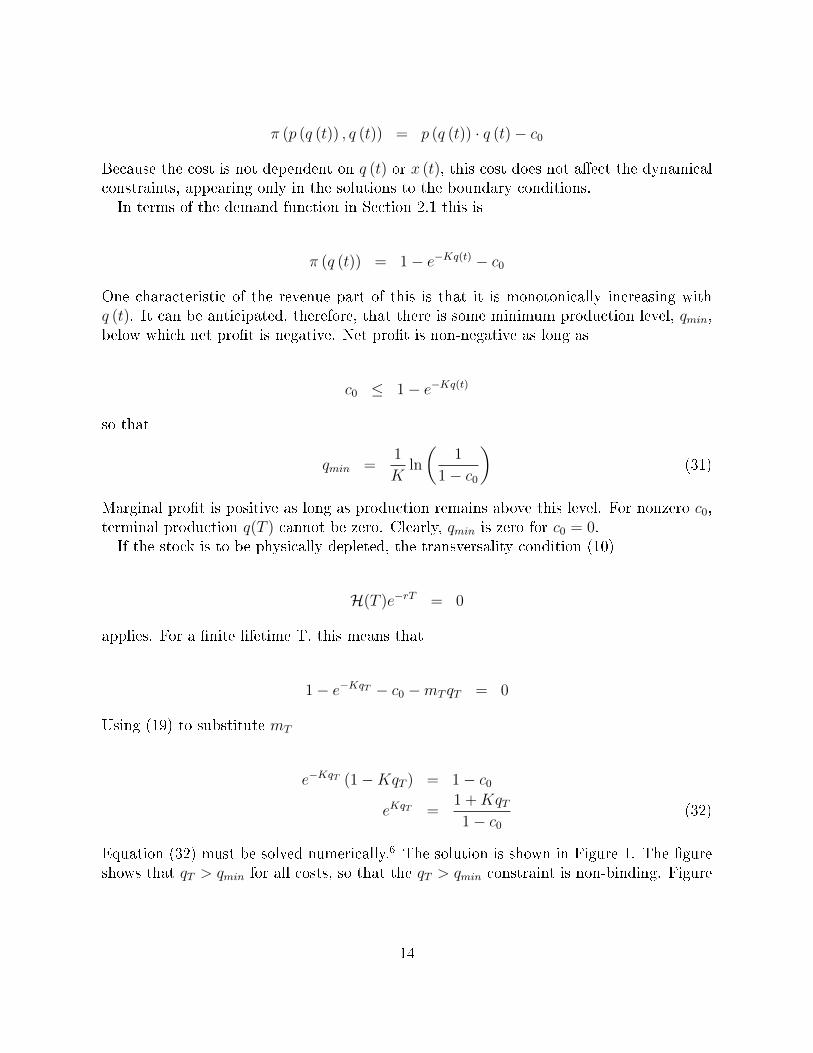
π (p (q (t)) , q (t)) = p (q (t)) · q (t)− c0

Because the cost is not dependent on q (t) or x (t), this cost does not a�ect the dynamicalconstraints, appearing only in the solutions to the boundary conditions.In terms of the demand function in Section 2.1 this is

π (q (t)) = 1− e−Kq(t) − c0

One characteristic of the revenue part of this is that it is monotonically increasing withq (t). It can be anticipated, therefore, that there is some minimum production level, qmin,below which net pro�t is negative. Net pro�t is non-negative as long as

c0 ≤ 1− e−Kq(t)

so that

qmin =1

Kln

(1

1− c0

)(31)

Marginal pro�t is positive as long as production remains above this level. For nonzero c0,terminal production q(T ) cannot be zero. Clearly, qmin is zero for c0 = 0.If the stock is to be physically depleted, the transversality condition (10)

H(T )e−rT = 0

applies. For a �nite lifetime T, this means that

1− e−KqT − c0 −mT qT = 0

Using (19) to substitute mT

e−KqT (1−KqT ) = 1− c0

eKqT =1 +KqT1− c0

(32)

Equation (32) must be solved numerically.6 The solution is shown in Figure 1. The �gureshows that qT > qmin for all costs, so that the qT > qmin constraint is non-binding. Figure

14

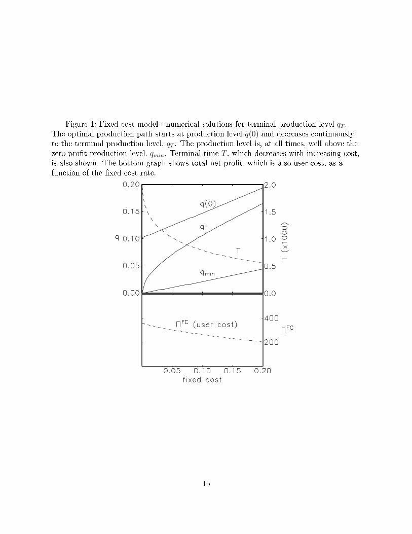
Figure 1: Fixed cost model - numerical solutions for terminal production level qT .The optimal production path starts at production level q(0) and decreases continuouslyto the terminal production level, qT . The production level is, at all times, well above thezero pro�t production level, qmin. Terminal time T , which decreases with increasing cost,is also shown. The bottom graph shows total net pro�t, which is also user cost, as afunction of the �xed cost rate.

15

1 also shows that terminal time T decreases sharply as cost increases, and that total netpro�t (user cost) decreases steadily over the cost range.Note, in Figure 1, that q(0) is slightly steeper than qmin, while qT is asymptotically

parallel to q(0). Thus, as the �xed cost increases, more of total production is pushedtoward the present.Replacing m0 in (21) with mT e

−rT

m (t) = m0ert = mT e

−rT ert

then using (19)

m (t) = Ke−KqT e−r(T−t)

so that

q (t) =1

Kln

[K

Ke−KqT e−r(T−t)

]= qT +

r

K(T − t) (33)

Thus, the initial production level is

q (0) = qT +rT

K(34)

which is also shown in Figure 1.Stock lifetime T is calculated from

x0 =

T

0

q (t) dt

= qTT +rT 2

2K

so that

T =K

r

(√q2T +

2rx0K− qT

)(35)

6The GAUSS code for numerical solutions is available from http://www.unm.edu/~ddixon (last ac-cessed 28 February 2010)

16

which is shown in Figure 1. Substituting (35) back into (34)

q (0) =

√q2T +

2rx0K

(36)

Total pro�t is

ΠFC =

T

0

(1− e−Kq(t) − c0

)e−rtdt

=1

r

[1− c0 − e−rT

(1− c0 + rTe−KqT

)](37)

which reduces to (30) for c0 = 0 (for which qT = 0). This is also shown in Figure 1.

2.4 A marginal cost model

Extractive technologies, like most production technologies, incur costs that are proportionalto the level of production. Scott (1967) uses a quarrying example to illustrate that economyof scale considerations at low levels of production, and problems of marketing, deliveryand storage at high levels of production, lead to a U-shaped marginal cost curve. Cobb-Douglas models in which production level appears are found in econometric models ofnickel (Stollery, 1983) and copper (Young, 1992), for example. Conrad and Clark (1987,p. 165) give an example of a linear marginal cost associated with disposal of pollutants.For simplicity, this model considers a stylized linear marginal cost with marginal cost c1,so that the net pro�t function is

π (p (q (t)) , q (t) , t) = p (q (t)) · q (t)− c1 · q (t)

In terms of the demand function in Section 2.1 this is

π (q (t)) = 1− e−Kq(t) − c1q (t) (38)

The transversality condition depends on whether or not q(t) can go to zero when t = T .There is no minimum production level qmin as long as the cost goes to zero faster than therevenue. This is the case as long as

e−Kq(t) ≤ 1− c1q (t) (39)

Figure 2 shows graphs of the left-hand and right-hand sides of (39) for the parameter valuespresented in Section 2.1. The graphs show that, for all marginal costs lower than the choke

17

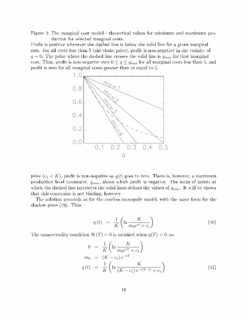
Figure 2: The marginal cost model - theoretical values for minimum and maximum pro-duction for selected marginal costs.

Pro�t is positive whenever the dashed line is below the solid line for a given marginalcost. For all costs less than 5 (the choke price), pro�t is non-negative in the vicinity ofq = 0. The point where the dashed line crosses the solid line is qmax for that marginalcost. Thus, pro�t is non-negative over 0 ≤ q ≤ qmax for all marginal costs less than 5, andpro�t is zero for all marginal costs greater than or equal to 5.

price (c1 < K), pro�t is non-negative as q(t) goes to zero. There is, however, a maximumproduction level constraint, qmax, above which pro�t is negative. The locus of points atwhich the dashed line intersects the solid lines de�nes the values of qmax. It will be shownthat this constraint is not binding, however.The solution proceeds as for the costless monopoly model, with the same form for the

shadow price (19). Thus

q (t) =1

K

(ln

K

m0ert + c1

)(40)

The transversality condition H (T ) = 0 is satis�ed when q(T ) = 0, so

0 =1

K

(ln

K

m0erT + c1

)m0 = (K − c1) e−rT

q (t) =1

K

(ln

K

(K − c1) e−r(T−t) + c1

)(41)

18

Unlike the costless and �xed cost models, the rate of change in the production path isnot constant, since

e−Kq(t) =(K − c1) e−r(T−t) + c1

K

−Kqe−Kq(t) =r (K − c1) e−r(T−t)

K(42)

qe−Kq(t) = − r

K

[(K − c1) e−r(T−t) + c1

K− c1K

]q = − r

K

[1− c1

KeKq(t)

](43)

The terminal time T is found by integrating

x0 =

T

0

1

Kln

K

(K − c1) e−r(T−t) + c1dt (44)

Kx0 =

T

0

lnK

(K − c1) e−r(T−t) + c1dt

Equation (44) is solved numerically in GAUSS using the parameters from Section 2.1.7

The numerical solution for T as a function of marginal cost is shown in Figure 3. Once Tfor a given marginal cost is known, the initial production level is determined from

q (0) =1

K

(ln

K

(K − c1) e−rT + c1

)(45)

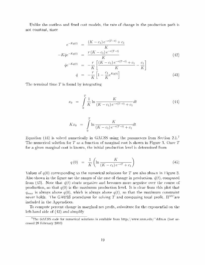
Values of q(0) corresponding to the numerical solutions for T are also shown in Figure 3.Also shown in the �gure are the ranges of the rate of change in production, q(t), computedfrom (43). Note that q(t) starts negative and becomes more negative over the course ofproduction, so that q(0) is the maximum production level. It is clear from this plot thatqmax is always above q(0), which is always above q(t), so that the maximum constraintnever holds. The GAUSS procedures for solving T and computing total pro�t, ΠMCareincluded in the Appendices.To compute percent change in marginal net pro�t, substitute for the exponential on the

left-hand side of (42) and simplify

7The GAUSS code for numerical solutions is available from http://www.unm.edu/~ddixon (last ac-cessed 28 February 2010)

19

Figure 3: Marginal cost model - numerical solutions for terminal time T.T is solved numerically from equation (44). Initial production level q(0) is solved using T .Also shown is the production maximum qmax computed from equation (39) using theequality condition. The lower graph shows the production rate of change as a function ofmarginal cost, with the arrow depicting the trajectory over time for a speci�c marginalcost. Also shown in the bottom plot is total pro�t as a function of marginal cost.

20

−Kq (K − c1) e−r(T−t) + c1K

=r (K − c1) e−r(T−t)

K

q = − r

K

(K − c1) e−r(T−t)

(K − c1) e−r(T−t) + c1

= − r

K

(1 +

c1K − c1

er(T−t))−1

From this it is obvious both that the magnitude of the rate of change decreases withincreasing c1, and that the magnitude increases over time for a given c1. Finally,

πqπq

=−K2qe−Kq(t)

Ke−Kq(t) − c1

= −Kq K

K − c1eKq(t)

= −K[− r

K

[1− c1

KeKq(t)

]] [ K

K − c1eKq(t)

]= r

[K − c1eKq(t)

K

] [K

K − c1eKq(t)

]= r

which is Hotelling's Rule.

2.5 A stock cost model

Stock costs - costs associated with cumulative production - are mentioned speci�cally byHotelling (1931, p. 152) as a detail omitted from his model. Stock e�ects appear in manyforms in natural resource production models. Lecomber (1979, p 54) sites the examples ofdecreasing pressure over the lifetime of an oil well, increased transportation costs as a minebecomes deeper, and a reduction in yield as the quality of ore decreases.8 Like marginalcost models, stock cost models are often quadratic or in Cobb-Douglas form (Young, 1992).The functional forms of stock e�ects in general vary broadly. In �shery models, for ex-

ample, the stock variable may appear in the growth function as second-degree polynomials(Hanley et al., 1997, sec. 7.4). In econometric analysis of oil production in the U.K.,Pesaran (1990) �nds that production cost is inversely proportional to remaining stock.Pindyck (1978) presents a production model that includes growth from exploration, and�nds an inverse relation between exploration and stock. Slade (1982) �nds evidence of a

8Slade (1984) also points out that yield in copper mining depends on price: when the price is high,more expensive processing is used, which increases the yield.

21

cost curve that is U-shaped in cumulative production. Tietenberg and Lewis (2000, p. 149)present a resource model for which the stock cost is linear with cumulative production.For simplicity, this model employs a stock cost that is linear in the stock variable x (t).

The stock cost cS is

cs (x(t)) = c2 (x0 − x(t)) (46)

where c2 is the marginal cost of stock depletion. Note that

x0 − x(t) =

tˆ

0

q(t′)dt′

so that cS is identical to a cost based on cumulative production.The net pro�t function is

π (p (q (t)) , q (t) , t) = p (q (t)) · q (t)− c2 (x0 − x(t))

which, for the inverse demand function in Section 2.1, is

π (q (t) , x (t)) = 1− e−Kq(t) − c2 [x0 − x (t)] (47)

Coming into the pro�t function via the state variable x(t) means that

πx = c2 (48)

Unlike the preceding models, the general form of Hotelling's Rule (13) applies rather than(14).With cost based on cumulative production, it is possible for marginal cost to exceed

marginal pro�t as the stock diminishes. Again it is necessary to invoke the non-negativepro�t constraint, but unlike the �xed cost and marginal cost models, this constraint canbe binding.If production is to halt when cost exceeds revenue, the producer will optimize such that

(47) is non-negative at all times. For some values of c2, this can be maintained until thestock is physically depleted, and terminal shadow price can be positive. In other cases,however, this results in production ceasing before the stock is physically depleted, so thatx (T ) > 0. In this case, the transversality condition (9) requires that m (T ) = 0.The �rst order necessary condition for Hq proceeds as for the costless model up to (20).

From the �rst order necessary condition for Hx (11)

m (t) = rm (t)− c2

22

This di�erential equation has the solution

m (t) =c2r

(1− ert

)+ Cert

where C is a constant of integration. Solving for C using the yet-to-be-determined terminalshadow price mT ,

m (t) =c2r

[1− e−r(T−t)

]+mT e

−r(T−t) (49)

Note that the static solution to the di�erential equation, in which rm (t) = c2, is recoveredfor m0 = mT = c2/r. It will be seen that this static condition represents the transitionfrom decreasing to increasing production path.Assuming that T is nonin�nite, there are two forms for the terminal Hamiltonian, de-

pending on whether x (T ) = 0 or x (T ) > 0. For x (T ) = 0, m (T ) > 0, so

H (T ) = 1− e−Kq(T ) − c2x0 −mT q (T ) = 0

which yields

e−Kq(T ) =1− c2x0

1 +Kq (T )(50)

This has a unique solution for q (T ) given c2, as long as c2 <1x0. This is solved numerically

in GAUSS.9

The condition x (T ) > 0 arises because marginal pro�t becomes negative before the stockis physically depleted. Marginal pro�t going to zero implies also that shadow price of thenext unit of resource is zero. That is, m (T ) = 0, which is the transversality condition forx (T ) > 0. Pro�t going to zero provides an additional constraint on q (T ),

1− e−Kq(t) − c2 [x0 − x (T )] = 0 (51)

The �rst order necessary condition (19) implies that, if m (T ) = 0, then e−Kq(T ) = 0, sothat (51) becomes

x (T ) = x0 −1

c2(52)

Clearly, this only holds for c2 ≥ 1x0. Thus, c2 = 1

x0marks the transition between physical

depletion of the stock with a non-zero terminal shadow price, and economic depletion, withsome physical stock remaining and a zero terminal shadow price. That is

9The GAUSS code for numerical solutions is available from http://www.unm.edu/~ddixon (last ac-cessed 28 February 2010)

23

m (T ) > 0 , x (T ) = 0 for c2 <1x0

m (T ) = 0 , x (T ) > 0 for c2 >1x0

Finally, in this regime, the terminal Hamiltonian is

H (T ) = 1− c2 (x0 − x (T )) = 0

which is satis�ed by the terminal stock level (52). Finally, terminal time T is found byintegrating

x0 − x (T ) =

T

0

q (t) dt (53)

where

q (t) =1

Kln

Kc2r

[1− e−r(T−t)] +mT e−r(T−t)(54)

The numerical solutions for the x (T ) = 0 regime involve solving for q (T ) using (50),computing m (T ) from (19), then numerically integrating (54) to �nd the T that solves(53) with x (T ) = 0. For the x (T ) > 0 regime, mT is assumed zero, and (54) is integratedto �nd the T that solves (53) where x (T ) is found using (52).On a �nal note, (13) implies that the percent change in marginal net pro�t changes over

time, since πx is constant while πq, equation (18), is a function of time . The percentchange in marginal net pro�t is positive for

r >πxπq

=c2

Ke−Kq(t)

percent change in marginal net pro�t is computed from the derivative of πq with respectto time

πqπq

=ddtKe−Kq(t)

Ke−Kq(t)= −Kq (55)

where q is the time rate of change in production. This is found by taking the derivative of(19) with respect to time

24

Figure 4: Stock cost model - theoretical values for terminal time, initial production level,starting and ending shadow price, ending stock level, producer pro�t, and usercost as a function of stock cost.

The top plot shows the numerical solutions for initial production q (0), starting shadowprice m (0) and ending shadow price m (T ) as a function of stock cost parameter c2.The middle plot shows the numerical solutions for terminal stock x (T ), total producerpro�tΠSC , and user cost as a function of c2. The bottom plot shows termination time T ,percent change in marginal net pro�t and percent change in marginal net pro�t plus stockcost. This last value should equal the discount rate (see equation 13).

25

d

dtKe−Kq(t) =

d

dtm (t)

−K2qe−Kq(t) = m

Substituting (12) into the left hand side and (11) into the right hand side

−Km (t) ˙q (t) = rm (t)− c2˙q (t) = − 1

K

(r − c2

m (t)

)= − r

K

(1− c2

rKekq(t)

)For small enough c2, the production path will be downward sloping. For higher c2, it willbe upward sloping. Substituting back into the percent change in marginal net pro�t (55)

πqπq

= r − c2m (t)

(56)

Finally, replacing c2 from (48) and m(t) from (12),

πqπq

= r − πxπq

This is Hotelling's Rule for nonzero stock cost as seen in (13). π/π in Figure 4 is computedusing (56).

2.6 Oligopoly models

Perhaps the most straightforward de�nition of an oligopoly market is in terms of what itis not. It is not a monopoly market - there is more than one producer. Nor is it a com-petitive market, if a competitive market is de�ned as one in which there is a large numberof producers, no one of which can a�ect the market equilibrium when acting indepen-dently. There are only a few ways in which an oligopoly producer can a�ect equilibrium,however, each depending on the reaction of the rest of the producers in the market. Forexample, total pro�t is maximized in a monopoly market, so if all the oligopolists canagree to hold their combined production to the monopoly level, the average pro�t per pro-ducer is maximum. This is a collusion market. At the other extreme, they can engage inprice competition, driving the price down to marginal cost and eliminating economic pro�taltogether, and possibly driving higher-cost producers out of the market. This is the out-come of the price-competition, or Bertrand, oligopoly model. The other possible outcomes

26

are modeled based on quantity competition (Cournot oligopoly model), market leadership(Stackelburg oligopoly model) or product di�erentiation (Bertrand oligopoly with productdi�erentiation). These models have the distinction of giving the producers levels of pro�tintermediate between collusion and perfect competition.Qualitatively, the expectations of an oligopoly market are:

• If the total production path is similar to the monopoly production path, it is acollusive market

• If total production is high and market price trends down to marginal cost then pricecompetition is occurring

• If total production is higher than monopoly but lower than price competition, thenthere is production-level cooperation (Cournot or Stackelburg) or price competitionwith product di�erentiation (Bertrand).

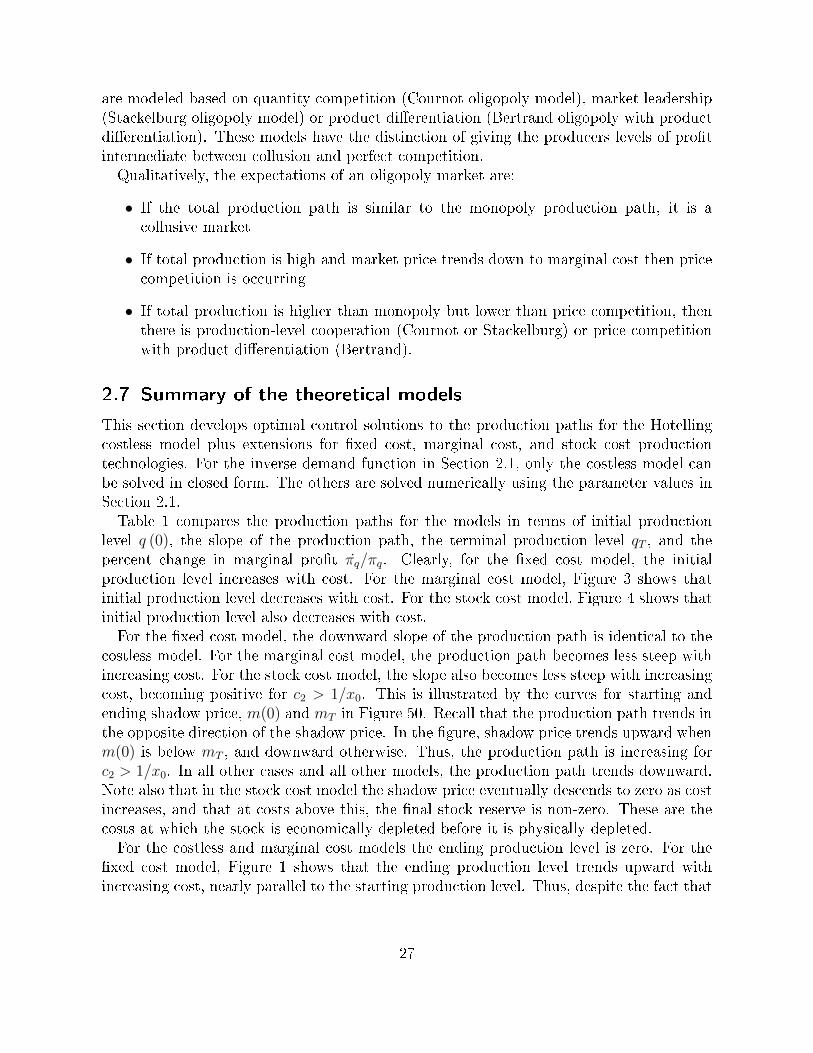
2.7 Summary of the theoretical models

This section develops optimal control solutions to the production paths for the Hotellingcostless model plus extensions for �xed cost, marginal cost, and stock cost productiontechnologies. For the inverse demand function in Section 2.1, only the costless model canbe solved in closed form. The others are solved numerically using the parameter values inSection 2.1.Table 1 compares the production paths for the models in terms of initial production

level q (0), the slope of the production path, the terminal production level qT , and thepercent change in marginal pro�t πq/πq. Clearly, for the �xed cost model, the initialproduction level increases with cost. For the marginal cost model, Figure 3 shows thatinitial production level decreases with cost. For the stock cost model, Figure 4 shows thatinitial production level also decreases with cost.For the �xed cost model, the downward slope of the production path is identical to the

costless model. For the marginal cost model, the production path becomes less steep withincreasing cost. For the stock cost model, the slope also becomes less steep with increasingcost, becoming positive for c2 > 1/x0. This is illustrated by the curves for starting andending shadow price, m(0) and mT in Figure 50. Recall that the production path trends inthe opposite direction of the shadow price. In the �gure, shadow price trends upward whenm(0) is below mT , and downward otherwise. Thus, the production path is increasing forc2 > 1/x0. In all other cases and all other models, the production path trends downward.Note also that in the stock cost model the shadow price eventually descends to zero as costincreases, and that at costs above this, the �nal stock reserve is non-zero. These are thecosts at which the stock is economically depleted before it is physically depleted.For the costless and marginal cost models the ending production level is zero. For the

�xed cost model, Figure 1 shows that the ending production level trends upward withincreasing cost, nearly parallel to the starting production level. Thus, despite the fact that

27

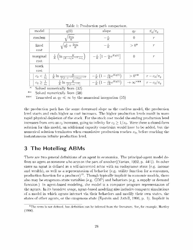
Table 1: Production path comparison.

model q(0) slope qT πq/πq

costless√

2rx0K

− rK

0 r

�xedcost

√q2T + 2rx0

K− rK

> 0* r

marginalcost

1K

(ln K

(K−c1)e−rT+c1

)− rK

[1− c1

KeKq(t)

]0 r

stockcost

c2 <1x0

1K

ln Kc2r[1−e−rT ]+mT e−rT − r

K

(1− c2

rKeKq(t)

)> 0** r − c2/πq

c2 ≥ 1x0

1K

ln Kc2r[1−e−rT ]

− rK

(1− c2

rKeKq(t)

)→∞*** r − c2/πq

* Solved numerically from (32)** Solved numerically from (50)*** Truncated at qT �∞ by the numerical integration (53)

the production path has the same downward slope as the costless model, the productionlevel starts and ends higher as cost increases. The higher production levels result in morerapid physical depletion of the stock. For the stock cost model the ending production levelincreases from zero as c2 increases, going to in�nity for c2 ≥ 1/x0. Were there a closed-formsolution for this model, an additional capacity constraint would have to be added, but thenumerical solution terminates when cumulative production reaches x0, before reaching theinstantaneous in�nite production level.

3 The Hotelling ABMs

There are two general de�nitions of an agent in economics. The principal-agent model de-�nes an agent as someone who acts on the part of another((Varian, 1992, p. 441)). In othercases an agent is de�ned as a self-interested actor with an endogenous state (e.g. incomeand wealth), as well as a representation of behavior (e.g. utility function for a consumer,production function for a producer)10. Though typically implicit in economic models, therealso may be exogenous state variables (e.g. GDP) and behaviors (e.g. a supply or demandfunction.) In agent-based modeling, the model is a computer program representation ofthe agents. In its broadest usage, agent-based modeling also includes computer simulationsof a model in which agents interact via their behaviors and modify their own states, thestates of other agents, or the exogenous state (Epstein and Axtell, 1996, p. 4). Implicit in

10The term is not de�ned, but de�nition can be inferred from the literature. See, for example, Hartley(1996).

28

agent-based modeling is that the agents are autonomous (Tesfatsion, 2006, p. 843).The agents in the ABM in this paper have no information about the demand function

itself, each determining autonomously its own optimal production path. The extent of theresource is known exactly, but the market structure and demand function are unknown.These are adaptive agents for which the behavioral rule is a heuristic to continually adjustthe production level so that estimated total pro�t is maximized. Pro�t estimates are basedon the observed market response to changes in production level. In addition to the costlessbasic models, there are models with non-zero cost which may be constant (per period),marginal (per unit production) or cumulative (proportional to the stock level).The models are constructed and the simulations run using the MASON agent-based

modeling and simulation library and framework. They are based on and incorporated intoa set of programs included with MASON to demonstrate the MASON Console environment.The Console provides a general graphical interface for editing model parameters, runningsimulations and for viewing model variables as time-series graphs or numerical tables.The graphical interface for each Hotelling model provides the ability to select a demand

function and one of the various market models described in the following sections, allowingthe user to change the number of producers in the market. Once a speci�c demand functionand market model has been selected, the user can change model-speci�c variables, suchas the mean and standard deviation for cost variables, for example. While running, thesimulation displays a custom window showing real-time plots of current pro�t, currentpercent change in marginal pro�t, stock level and production level. Each model optionallywrites a �le of key dynamical variables. These �les were used to produce the plots presentedin Section 4. Images of the interface and results windows are included in the Appendices.Each model has two types of agent: a market agent and a producer agent. In a given

model there is a single market agent and one or more producer agents. The simulationis initialized with Monte Carlo draws for the stochastic variables, then the simulationproceeds, one time-step at a time, until all producers have stopped. The producers stopeither because the resource stock level is zero, or pro�t in the current period is negative.11

Because the agents are autonomous, the simulation behaviors are mediated by informationthat is communicated between agents, speci�cally between each �rm agent and the marketagent. These exchanges occur as four distinct actions during each time-step, as illustratedin Figure 5. The size of a simulation time-step is arbitrary, though the default discountrate is assumed daily and compounds to ten percent per annum. Changing the discountrate, via the GUI, changes the implied time-step.

11In some models, pro�t goes negative even though an alternative production level would producepositive pro�t. A more advanced heuristic could explore alternative production levels to determine if thisis the case, but the simple heuristic does not. This is not dissimilar to a situation in which the ownerof the resource prefers to shut down leaving a small reserve rather than take the risk of incurring furthernegative pro�ts while searching for a pro�table production path.

29

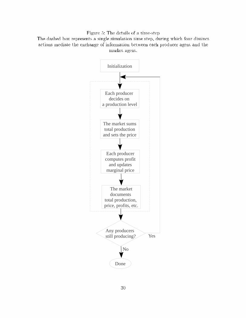
Figure 5: The details of a time-stepThe dashed box represents a single simulation time-step, during which four distinctactions mediate the exchange of information between each producer agent and the

market agent.

Each producer decides on

a production level

Initialization

The market sumstotal production

and sets the price

Any producersstill producing?

Done

The marketdocuments

total production, price, profits, etc.

Each producercomputes profit

and updatesmarginal price

Yes

No

30

3.1 The market agent

The market agent, called Market, is assigned a demand function and controls any marketinformation provided to the producers. Both the speci�c market agent and the demandfunction are user-selectable: changing from one model to another is simply a matter ofchanging the market agent and/or the market agent's demand function. The market agentrepresents a speci�c market structure and production technology. For example, there is acostless market agent, a �xed-cost market agent, an oligopoly market agent and so on.

3.2 The producer agent

In contrast, the producer agent, called Firm, is the same for all models. The producer agentcomputes pro�t, marginal price, marginal pro�t and the percent change in marginal pro�tfor each time period. This information is used by the producer agent at the beginning ofeach time period to compute the next production level and is collected at the end of eachtime period by the market agent for the real-time displays and, optionally, written to a �lefor post-processing.Although the producer is the optimizing agent, the algorithms to compute future pro�t

are contained in the market agent so that the details can vary depending on the marketmodel. A simple heuristic is used for optimization and is described in the next section.

3.3 A simple optimization heuristic

The �rst step in designing the model is to �nd an optimization heuristic that is as simpleas possible while reproducing plausible behavior. Algorithmic simplicity contributes torobustness, that is, the ability to produce consistent behavior under the planned variety ofproduction technologies and market structures. For example, in a tournament of biddingalgorithms, Rust et al. (1992) found that the simplest algorithms consistently beat themore complex. Another advantage to simplicity is analytic transparency. The di�cultyin associating speci�c outcomes with speci�c behaviors increases as the complexity ofthe algorithms increases. From an experimental control perspective, it is also easier todetect, explain and compute the impact of algorithmic artifacts for a simple algorithm.Algorithmic artifacts may results from the size of the simulation time-step, the size ofchanges in production level, or numerical errors in calculating pro�t, cost or productionlevel changes. A possible added bene�t of a simple algorithm is shorter computation times,since proper Monte Carlo sampling calls for large numbers of simulations.The core of the heuristic is a simple estimation of future pro�t. The heuristic uses the

pro�t estimation in two di�erent ways, depending on the phase of the simulation. Thephases are:

1. Increase production level from zero until estimated future pro�ts begin to fall. Thisis called the ramp-up phase.

31

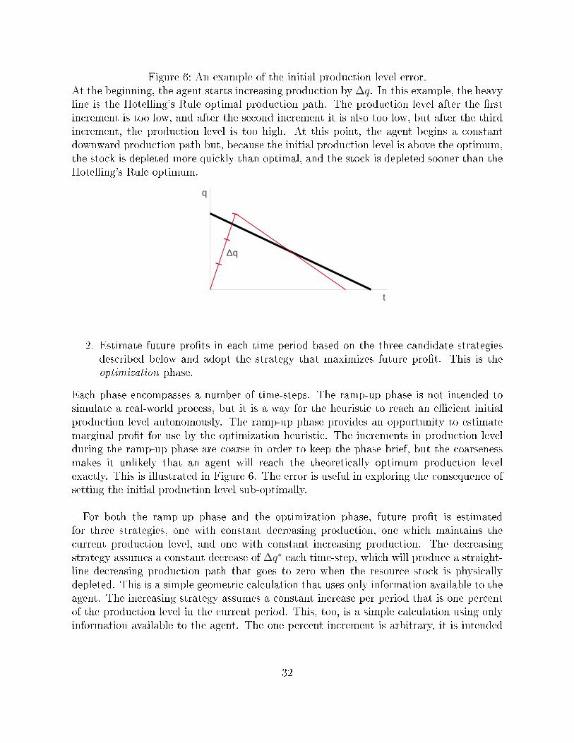
Figure 6: An example of the initial production level error.At the beginning, the agent starts increasing production by ∆q. In this example, the heavyline is the Hotelling's Rule optimal production path. The production level after the �rstincrement is too low, and after the second increment it is also too low, but after the thirdincrement, the production level is too high. At this point, the agent begins a constantdownward production path but, because the initial production level is above the optimum,the stock is depleted more quickly than optimal, and the stock is depleted sooner than theHotelling's Rule optimum.

t

q

Δq

2. Estimate future pro�ts in each time period based on the three candidate strategiesdescribed below and adopt the strategy that maximizes future pro�t. This is theoptimization phase.

Each phase encompasses a number of time-steps. The ramp-up phase is not intended tosimulate a real-world process, but it is a way for the heuristic to reach an e�cient initialproduction level autonomously. The ramp-up phase provides an opportunity to estimatemarginal pro�t for use by the optimization heuristic. The increments in production levelduring the ramp-up phase are coarse in order to keep the phase brief, but the coarsenessmakes it unlikely that an agent will reach the theoretically optimum production levelexactly. This is illustrated in Figure 6. The error is useful in exploring the consequence ofsetting the initial production level sub-optimally.

For both the ramp-up phase and the optimization phase, future pro�t is estimatedfor three strategies, one with constant decreasing production, one which maintains thecurrent production level, and one with constant increasing production. The decreasingstrategy assumes a constant decrease of ∆q∗ each time-step, which will produce a straight-line decreasing production path that goes to zero when the resource stock is physicallydepleted. This is a simple geometric calculation that uses only information available to theagent. The increasing strategy assumes a constant increase per period that is one percentof the production level in the current period. This, too, is a simple calculation using onlyinformation available to the agent. The one percent increment is arbitrary, it is intended

32

to be small, thus preventing large swings in production level. It is also advantageousthat it be di�erent in magnitude from the decreasing strategy, reducing the likelihood ofnon-damping oscillations.

3.4 The use of discrete summations

The following sections present the calculations used by the agents to determine the bestoptimization strategy. In contrast to the integrals presented in Section 2, these are discretesummations, and the derivatives are all discrete (e.g.∆q, ∆p, ∆π). This re�ects the factthat the simulation itself employs discrete time. A producer agent has very little infor-mation and estimates future pro�t by counting up the discounted pro�t per period untilthe stock is physically depleted. Further advantage is taken of the fact that the produceragent's strategies all assume constant changes to the production level ∆q, so that theamount of the change itself comes out of the summations.The discrete summations also have the advantage of allowing for variable time steps.

The simulations presented here all assume planning on a daily basis, which is may not berealistic. A real-world planner may reassess the production plan once a quarter or once peryear. To simulate these planning periods, the user of these simulations need only changethe discount rate from daily to quarterly or annual.

3.5 The heuristic algorithm

Estimated future pro�t is computed with all production in the future and pro�t discountedaccordingly. For a costless model, the future pro�t calculation is the summation

Πτ =τ−1∑i=0

qipi (1 + r)−i

where

Πτ = estimated future pro�t

qi = production level in period i

pi = price in period i

r = discount rate

τ = remaining lifetime of the stock

With a constant change in production level 4q � which can be negative, positive, orzero � the production level in period i is

qi = qn + i4q

33

where qn is the base production level, meaning the production level at the time the esti-mate is being computed, and i enumerates the production periods into the future. Theproduction period i starts at zero for the current production period n. Because the inversedemand function is unknown to the agent, price is estimated based on the most recentmarginal price

pi = pn +4qi(4p4q

)i−1

where pn is the price in the current period, and

(4p4q

)i−1

=pi−1 − pi−2qi−1 − qi−2

(57)

is the estimated marginal price based on price and production level changes between theprevious two periods. Estimated future pro�t becomes

Πτ (4q) =τ−1∑i=0

(qn + i4q)[pn + i4q

(4p4q

)i−1

](1 + r)−i

= qnpnA+4q[pn + qn

(4p4q

)i−1

]B + (4q)2

(4p4q

)i−1

C (58)

where

A =τ−1∑i=0

(1 + r)−i =1 + r

r

[1− (1 + r)−τ

](59)

B =τ−1∑i=0

i (1 + r)−i =1

r

[A− τ

(1 + r)τ−1

](60)

C =τ−1∑i=0

i2 (1 + r)−i =1

r

[2B + A− τ 2

(1 + r)τ−1

](61)

The lifetime of the remaining stock comes from the constraint that total productionequal total current stock

xn =τ−1∑i=0

(qn + i4q) = τqn +4q τ (τ − 1)

2

τ =−(qn − 4q2

)+

√(q − 4q

2

)2+ 2xn4q

4q(62)

34

where xn is the reserve stock in the current period. There exists some minimum constantproduction change ∆q∗ for which the total remaining stock is exhausted, at which pointproduction goes to zero. The lifetime in this case is constrained by

qn +τ−1∑i=0

∆q∗ = 0 (63)

and the constraint that total production equal the current stock by

τ−1∑i=0

(qn + i∆q∗) = xn (64)

Solving (63) for ∆q∗ and substituting into (64)

τ =2xnqn− 1 (65)

Substituting this back into (63),

∆q∗ = − q2n2xn − qn

(66)

This is the lowest (most negative) 4q that will result in a straight-line decreasing produc-tion path for which production goes to zero as the stock is physically depleted. This alsosatis�es the constraint that the term in the radical in (62) be non-negative.

3.6 Costless model

Initially, consistent with Hotelling, costless production is considered. The introduction ofnonzero cost will be presented in Section 3.7. Production decisions use a heuristic thatestimates future pro�t as described in Section 3.3.The theoretical maximum pro�t is shown in (30). The equivalent summation expression

is

Πmax =T−1∑i=0

(1− e−Kqi

)(1 + r)−i =

1 + r

r

[1− (1 + r)−T

]− (1 + r)−T − e−rT

er (1 + r)−1 − 1(67)

With the values given in Section 2.2, the discrete Πmax = 358.53, as compared to thecontinuous Πmax = 358.33, the di�erence being due to numerical errors. In practical

35

terms, the monopoly models are special cases of the oligopoly models, so simulation resultsof the monopoly models are discussed in their respective oligopoly sections in Section 4.A producer agent has no knowledge of the demand function, and can only infer it from the

observed behavior of the market. Namely, the change in price that results from changes inthe production level. The agent has two behavioral rules, corresponding to the two phasesof the heuristic:

Rule 1. In the ramp-up phase, increase the production level from zero until estimatedtotal pro�t is positive and begins to decrease. The default monopoly ramp-uprate is an increase of 0.01 units of production per period.

Rule 2. In the optimization phase, in each period, estimate future pro�t based onthe three production strategies, then execute the strategy that maximizesfuture pro�t. Production ceases if, after the ramp-up phase, pro�t becomesnegative.

3.7 Production technologies with nonzero cost

The production technology models with nonzero cost are the costless model with a nonzerocost term. This does not require a change in the producer agent, which is implementedwith cost variables, all of which were zero for the costless model.

3.7.1 Fixed cost model

Recall from Section 2.3 that, for the �xed cost model, there is a minimum production levelqmin below which pro�t is negative. For the discrete calculations used by the heuristic, theconstraint (63) becomes

qn +τ−1∑i=0

∆q∗ = qmin (68)

which, when substituted into equation (64), means that equation (66) becomes

4q∗ =q2n − q2min

2xn − qn + qmin(69)

This is the minimum (most negative) change in production that results in a straight-line decreasing production path that reaches qmin at the moment the stock is physicallydepleted. The heuristic determines qmin by increasing production starting from zero andrecording the production level at which pro�t becomes positive.The estimate of future pro�t is

36

ΠFCτ = ΠNC

τ − c0τ−1∑i=0

(1 + r)−i

= ΠNCτ − c0A

where ΠNCτ is the no-cost future pro�t estimate (58) and A is from (59).

A �xed cost does not appear in πq or πx, so according to equation (13), there is no e�ecton the optimal percent change in marginal pro�t. The optimal production path is a�ected,however, since the initial production level q(0) and the terminal production level qT bothincrease with cost, as shown in Figure 1.

3.7.2 Marginal cost model

With no minimum production level constraint, the marginal cost model is identical to thecostless model. The change comes in the estimate of future pro�t

ΠMCτ = ΠNC

τ − c1τ−1∑i=0

(qn + i∆q) (1 + r)−i

= ΠNCτ − c1

[qn

τ−1∑i=0

(1 + r)−i + ∆qτ−1∑i=0

i (1 + r)−i]

= ΠNCτ − c1 (qnA+ ∆qB)

where ΠNCτ is the costless future pro�t estimate (58) and A and B are from equations (59)

and (60).

3.7.3 Stock cost model

With the addition of a stock cost as in (46), the future pro�t estimate becomes

ΠSCτ = ΠNC

τ −τ−1∑i=0

c2 (x0 − xi) (1 + r)−i

= ΠNCτ − c2x0

τ−1∑i=0

(1 + r)−i + c2

τ−1∑i=0

xi (1 + r)−i

= ΠNCτ − c3

τ−1∑i=0

(1 + r)−i + c2

τ−1∑i=0

(xn + ∆xi) (1 + r)−i (70)

where c3 ≡ c2x0. The discrete form of equation (6) is ∆x = −q. Assuming that q ischanging by the constant increment ∆q, then ∆xi = − (qn + i∆q). Now, (70) becomes

37

ΠSCτ = ΠNC

τ − (c3 − c2xn)τ−1∑i=0

(1 + r)−i − c2τ−1∑i=0

(qn + i∆q) (1 + r)−i

= ΠNCτ − (c3 − c2xn + c2qn)

τ−1∑i=0

(1 + r)−i − c2∆qτ−1∑i=0

i (1 + r)−i

= ΠNCτ − [c3 − c2 (xn − qn)]A− c2B∆q

where ΠNCτ is the costless future pro�t estimate (58) and A and B are from (59) and (60).

3.8 Other sources of uncertainty

If the producer is not certain of the extent of the resource x0, the consequent error in thelifetime of the stock will a�ect estimates of future pro�ts. This, in turn, may a�ect theproduction strategy selected by the heuristic outlined above. Although the heuristic canadjust the rate of change as the stock is depleted, the total pro�t is sensitive to an error inthe initial production level. An initial quantity that is too high will, in general, result inthe resource being depleted too quickly, leaving unrealized pro�t in the future. An initialquantity that is too low will, in general, result in the resource being depleted too slowly,with unrealized pro�t in the present.Errors in x0 are similar to errors in the initial production level, so Monte Carlo sampling

in the neighborhood of the initial production level will give an indication of sensitivityto errors in x0. The relation between initial production level and initial stock is givenby equation (27). The coarseness of the heuristic strategy serves as a proxy for errors incomputing optima, including errors in x0. This is illustrated in the discussion in Section4.4.Other sources of uncertainty in the interest rate, in the demand function, and in the

production technology cost function could be explored in a similar manner. Uncertaintyin the demand function can take on various forms, the simplest being random errors inconstants and systematic errors in functional form. In the former, a su�ciently largesample reveals a constant variance while, in the latter, a large sample reveals variance thatchanges over the range of production. Uncertainty enters the cost function in ways similarto the demand function. Of particular interest are cases in which the production plannerincorrectly assumes costless production. These issues are beyond the scope of this paper.

4 Simulation results

The ABMs are oligopoly models for which the monopoly results are special cases. Theoligopoly simulations have one market agent and one or more producer agents, dependingon the number of producers in the market. The number of producers is a user-set variable

38

in the GUI. Each producer is unaware of the others. In terms of the ABM architecture,this is done by not providing any communication between producer agents.The ensemble simulations are models in which there are multiple producer agents and

multiple market agents. Each pair of producer agent and market agent behaves like amonopoly with dedicated stock and a dedicated market. Ensembles are a way to collectdata about large number of monopolists while running only one simulation. In thesemodels, the monopolists are all di�erent because each one has been given productiontechnology cost parameters drawn at random from statistical distributions. This methodof mapping the parameter space onto the outcome space is called Monte Carlo sampling.The �rst sections will discuss the costless oligopoly models. The monopoly model for

each production technology is presented as an oligopoly with one producer. The followingsections will address the ensemble models. The last section will examines the e�ciency ofthe heuristic by introducing intentional error into the initial production level.The models in the following sections are intentionally wrong. In these models the pro-

ducer always behaves as though it is a monopoly market, even though the models includeoligopolies of two to six producers. Given that a real-world producer is likely to makemistaken assumptions about the market structure, the object is to assess the worst caseoutcome of assuming no competitors whatsoever.

4.1 The costless oligopoly model

For the models in this section, the total stock is constant as the number of producersincreases. For a duopoly, each producer begins with a stock of x0/2, and with ten producers,each producer begins with a stock of x0/10. The duopoly production path in Figure 10re�ects a collusion-like outcome, as do models for N=3 and N=4. That is, the produceragents arrive at what looks like a collusive market structure using only the optimizationheuristic. For an oligopoly of �ve producers, however, something completely di�erentoccurs, as seen in Figure 9. In this model, after the ramp-up phase, some producers beginreducing production while others continue unchanged.This behavior is an emergent property of the heuristic. Initially, the total stock of 100 is

distributed among the �ve producers in near equal amounts, with small random deviations.In this model, the initial stock allocations are 20.11, 20.09, 19.90, 19.88, and 20.02 for Firm1 through 5, respectively. All �ve �rms conclude the ramp-up phase on day 53. At thispoint, Firms 1 and 2, with the largest allocations, select a decreasing strategy, while therest of the �rms select zero change strategies. That an individual producer chooses a �atproduction strategy is not unexpected. However, the decreases in production by the twolargest producers cause price increases that are su�cient for the remaining producers toestimate increasing pro�ts at constant production levels for the duration of their stocks.That is, Firms 3, 4, and 5 are self-optimizing to higher total production than the collusiveoutcome (as per Cournot-Nash equilibrium) by maintaining constant production levelswhile Firms 1 and 2 decrease theirs.The results for models with from one to ten producers are shown in Figure 10. As

39

the number of �rms increases, the production paths present evidence of what Hotellingcalls the �retardation of production under monopoly� (Hotelling, 1931, sec. 7) in that thelifetime of the stock decreases as the number of producers increases. The models with �ve,seven and ten producers show the Cournot-like outcome, while the rest show the collusion-like outcome. All of these models appear to reach the theoretically optimal pro�t. Thesemodels show that total collusion-level pro�ts are not necessarily an indicator of collusion.Note also, in Figure 10, the discontinuities in the percent change in marginal pro�t curveswhere producers change strategies at the end stock life.

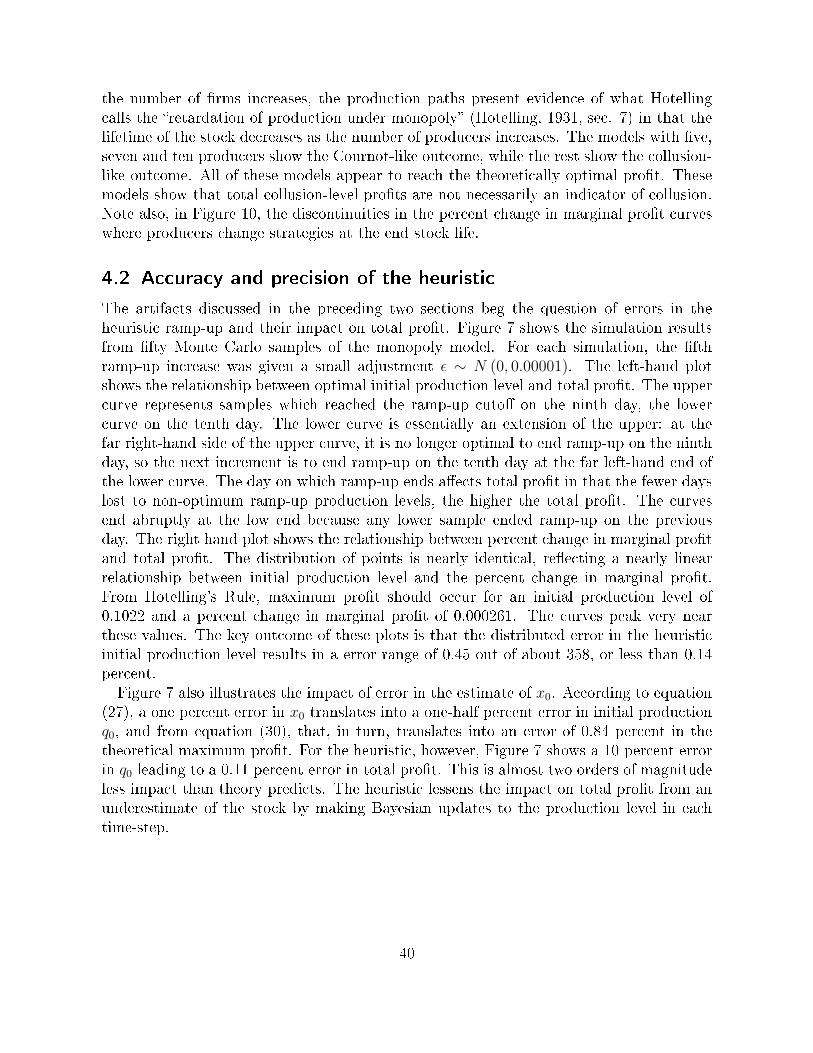
4.2 Accuracy and precision of the heuristic

The artifacts discussed in the preceding two sections beg the question of errors in theheuristic ramp-up and their impact on total pro�t. Figure 7 shows the simulation resultsfrom �fty Monte Carlo samples of the monopoly model. For each simulation, the �fthramp-up increase was given a small adjustment ε ∼ N (0, 0.00001). The left-hand plotshows the relationship between optimal initial production level and total pro�t. The uppercurve represents samples which reached the ramp-up cuto� on the ninth day, the lowercurve on the tenth day. The lower curve is essentially an extension of the upper: at thefar right-hand side of the upper curve, it is no longer optimal to end ramp-up on the ninthday, so the next increment is to end ramp-up on the tenth day at the far left-hand end ofthe lower curve. The day on which ramp-up ends a�ects total pro�t in that the fewer dayslost to non-optimum ramp-up production levels, the higher the total pro�t. The curvesend abruptly at the low end because any lower sample ended ramp-up on the previousday. The right hand plot shows the relationship between percent change in marginal pro�tand total pro�t. The distribution of points is nearly identical, re�ecting a nearly linearrelationship between initial production level and the percent change in marginal pro�t.From Hotelling's Rule, maximum pro�t should occur for an initial production level of0.1022 and a percent change in marginal pro�t of 0.000261. The curves peak very nearthese values. The key outcome of these plots is that the distributed error in the heuristicinitial production level results in a error range of 0.45 out of about 358, or less than 0.14percent.Figure 7 also illustrates the impact of error in the estimate of x0. According to equation

(27), a one percent error in x0 translates into a one-half percent error in initial productionq0, and from equation (30), that, in turn, translates into an error of 0.84 percent in thetheoretical maximum pro�t. For the heuristic, however, Figure 7 shows a 10 percent errorin q0 leading to a 0.11 percent error in total pro�t. This is almost two orders of magnitudeless impact than theory predicts. The heuristic lessens the impact on total pro�t from anunderestimate of the stock by making Bayesian updates to the production level in eachtime-step.

40

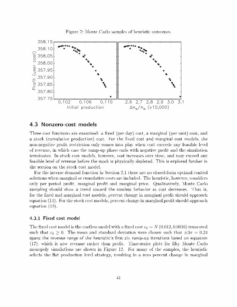
Figure 7: Monte Carlo samples of heuristic outcomes.

4.3 Nonzero-cost models

Three cost functions are examined: a �xed (per day) cost, a marginal (per unit) cost, anda stock (cumulative production) cost. For the �xed cost and marginal cost models, thenon-negative pro�t restriction only comes into play when cost exceeds any feasible levelof revenue, in which case the ramp-up phase ends with negative pro�t and the simulationterminates. In stock cost models, however, cost increases over time, and may exceed anyfeasible level of revenue before the stock is physically depleted. This is explored further inthe section on the stock cost model.For the inverse demand function in Section 2.1 there are no closed-form optimal control

solutions when marginal or cumulative costs are included. The heuristic, however, considersonly per period pro�t, marginal pro�t and marginal price. Qualitatively, Monte Carlosampling should show a trend toward the costless behavior as cost decreases. That is,for the �xed and marginal cost models, percent change in marginal pro�t should approachequation (14). For the stock cost models, percent change in marginal pro�t should approachequation (13).

4.3.1 Fixed cost model

The �xed cost model is the costless model with a �xed cost c0 ∼ N (0.012, 0.0016) truncatedsuch that c0 ≥ 0. The mean and standard deviation were chosen such that ±3σ = 0.24spans the revenue range of the heuristic's �rst six ramp-up iterations based on equation(17), which is now revenue rather than pro�t. Time-series plots for �fty Monte Carlomonopoly simulations are shown in Figure 12. For many of the samples, the heuristicselects the �at production level strategy, resulting in a zero percent change in marginal

41

pro�t until the �nal few time-steps. In other samples, the heuristic selects the decreasingstrategy followed by a �at strategy, resulting in percent change in marginal pro�t curvesthat sweep upward then fall to zero. The diamonds in the percent change in marginalpro�t plot indicate sharp spikes (to several hundreds on the scaled y-axis), indicating thatthe heuristic selects a rapid taper down to zero production over the �nal two or three time-steps as stock reaches physical depletion. Note that optimal percent change in marginalcost is 2.6 in this graph.The heavy dashed line in the production path plot indicates theoretical qmin from equa-

tion (31). This is the envelope for optimal terminal production levels.The results of the Monte Carlo monopoly simulations are summarized in Figure 15. Note

that the results cluster based on the heuristic qmin, and that qmin is in multiples of 0.01.This is because 0.01 is the default ramp-up production change and qmin is recorded by theheuristic during the ramp-up phase. The inset graph compares the heuristic values for qminwith the theoretical values from (31). The graphs show a distinct trend in percent changein marginal pro�t with regard to �xed cost. The dashed lines are the theoretical valuesdiscussed in Section 2.3.

4.3.2 Marginal cost model

The marginal cost model is the costless model with a constant marginal cost c1 ∼ N (1.0, 0.110889)truncated such that c1 ≥ 0. The time-series data for the marginal cost model are shownin Figure 13. The plot shows only three unique production paths because the initial valueis weakly dependent on marginal cost, and the step size in the ramp-up heuristic is muchgreater than the variations between starting production levels. The time-series data alsoreveal that percent change in marginal pro�t is always close to the optimal 2.6, and trendstoward it in the course of the simulation.The results from �fty Monte Carlo monopoly simulations are shown in Figure 16. In

these models, percent change in marginal pro�t is sensitive to the initial production level. Apercent change in marginal pro�t below optimum implies that the initial production levelis too low, preventing the heuristic from optimally reducing production each time step.Similarly, a percent change in marginal pro�t above optimum implies an initial productionlevel that is too high. In all cases, the percent change in marginal pro�t trends downward.

4.3.3 Stock cost model

The stock cost model is the costless model. In this model, the optimum production pathcan be either decreasing or increasing over time, depending on the value of the stock costparameter c2. Also, for higher values of c2 it is expected that production will stop beforethe stock is physically depleted. These characteristics are discussed in Section 2.5.Before Monte Carlo sampling the parameter space, it is instructive examine the classes

of behavior anticipated. Figure 14 shows a time-series plot for �ve representative valuesof stock cost. The stock cost parameter c2 is shown as �sc� in the legend. The zero cost

42

model is included for comparison and is identical to the costless monopoly model in Section4.1. The model with c2 = 0.001 is included to show the deviation of a small cost from thecostless model. The model with c2 = 0.005 is included to show the behavior in the vicinityof transition from decreasing production to increasing production discussed in Section 2.5in the discussion of Figure 4. The model with c2 = 0.010 is 1/x0, which is the cost at whichthe producer will begin to leave some of the stock unproduced as discussed in Section 2.5,and the model with c2 = 0.013 is included to show the behavior well into the regime forwhich the physical stock is greater than zero when production stops.Interesting to note here is that, for small stock cost (much less than 0.10) or large stock

cost (signi�cantly greater than 0.10), the production paths are fairly smooth. In the vicinityof 0.10, however, the heuristic makes frequent changes resulting in a highly volatile percentchange in marginal pro�t. The percent change in marginal cost plot has been smoothedwith a boxcar length of 100 days. Note also that, for smaller stock costs, the percent changein marginal pro�t turns toward negative in�nity very quickly, and, at least for 0.005, andthen comes down from positive in�nity thereafter. This arises because, in this period, theproduction level is very close to the zero marginal pro�t regime. Marginal pro�t appears inthe denominator of percent change in marginal pro�t, hence the switch between negativeand positive in�nity as marginal pro�t crosses through zero.Figure Figure (17) shows the outcome space results from 50 Monte Carlo samples with

stock cost taken from c2 ∼ N (0.01, 0.000016), truncated such that c2 ≥ 0. Very little canbe drawn from the percent change in marginal pro�t plot other than to note, as in thetime-series plot, that percent change in marginal pro�t can be highly dynamic. The pro�tand user cost plot shows that the heuristic is near optimal at zero stock cost and when stockcost is 0.10. The error in the heuristic is especially large in the range between zero and0.10. The initial production level plot provides a clue as to why: initial production levelsare consistently too high, resulting in lower pro�ts and an ine�ciently rapid reduction instock. Finally, the upper right plot shows the consequences: a much shortened lifetimefor stock costs below 0.10, and too much stock left unexploited for stock costs above 0.10.The dashed lines are the theoretical values, as discussed in Section 2.5.

4.4 Theoretical e�ciency

To put the foregoing results into perspective, Figure 8 shows the e�ect of error in the the-oretical costless model. These are families of curves of total net pro�t from the theoreticalcostless monopoly model in Section 2.2. The initial production level q0 is varied plus orminus 15 percent about the optimum of 0.1022. The production path slope is also varied sothat percent change in marginal pro�t varies plus or minus 15 percent about the optimumof 2.61× 10−4.The widely spaced diagonal lines (on the left in the left �gure, on the right in the right

�gure) result from the initial production level being so low that the downward slope of theproduction path reduces production to zero before the stock is physically depleted. Thisrepresents a gross error in production planning and not one likely to be seen in real-world

43

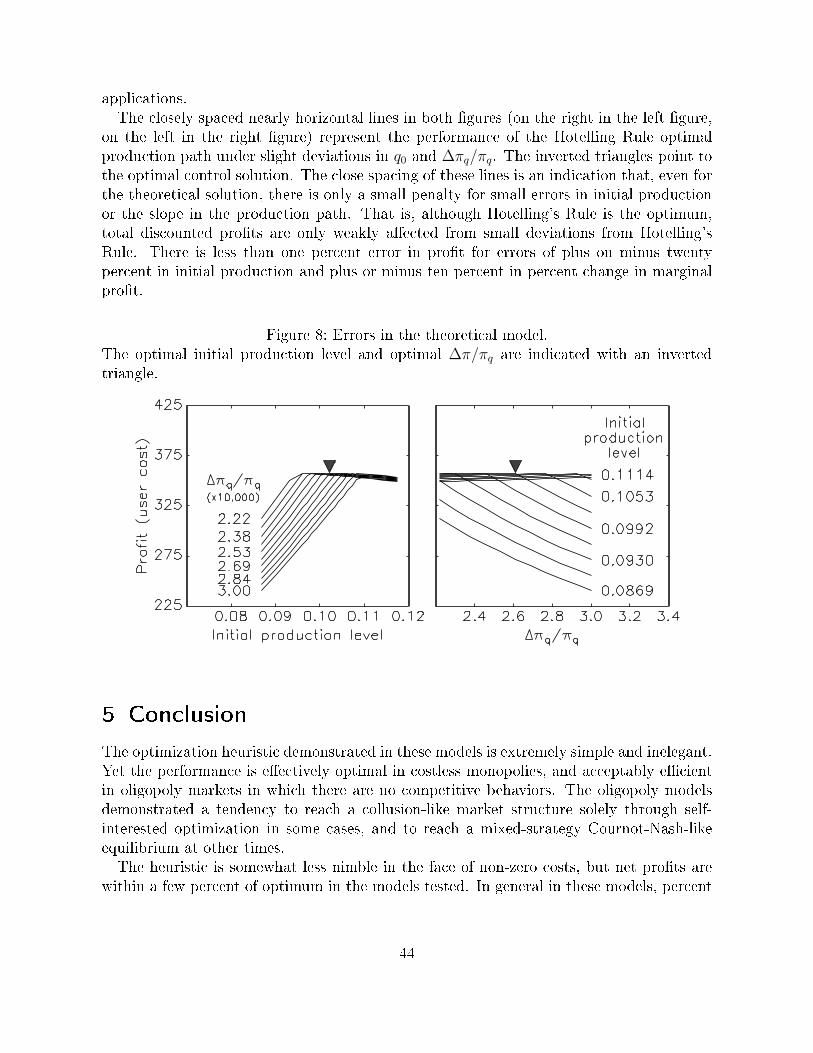
applications.The closely spaced nearly horizontal lines in both �gures (on the right in the left �gure,

on the left in the right �gure) represent the performance of the Hotelling Rule optimalproduction path under slight deviations in q0 and ∆πq/πq. The inverted triangles point tothe optimal control solution. The close spacing of these lines is an indication that, even forthe theoretical solution, there is only a small penalty for small errors in initial productionor the slope in the production path. That is, although Hotelling's Rule is the optimum,total discounted pro�ts are only weakly a�ected from small deviations from Hotelling'sRule. There is less than one percent error in pro�t for errors of plus on minus twentypercent in initial production and plus or minus ten percent in percent change in marginalpro�t.

Figure 8: Errors in the theoretical model.The optimal initial production level and optimal ∆π/πq are indicated with an invertedtriangle.

5 Conclusion

The optimization heuristic demonstrated in these models is extremely simple and inelegant.Yet the performance is e�ectively optimal in costless monopolies, and acceptably e�cientin oligopoly markets in which there are no competitive behaviors. The oligopoly modelsdemonstrated a tendency to reach a collusion-like market structure solely through self-interested optimization in some cases, and to reach a mixed-strategy Cournot-Nash-likeequilibrium at other times.The heuristic is somewhat less nimble in the face of non-zero costs, but net pro�ts are

within a few percent of optimum in the models tested. In general in these models, percent

44

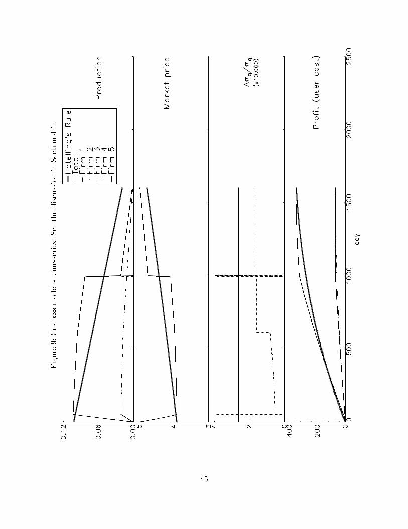
Figure

9:Costlessmodel-time-series.See

thediscussionin

Section

4.1.

45

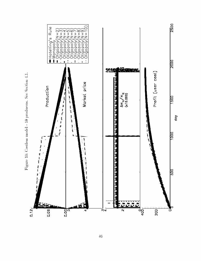
Figure

10:Costlessmodel-10

producers.See

Section

4.1.

46

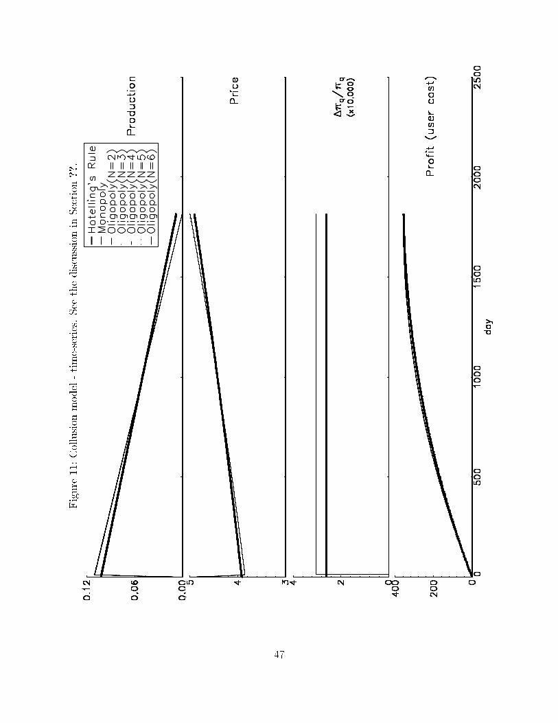
Figure

11:Collusion

model-time-series.See

thediscussionin

Section

??.

47

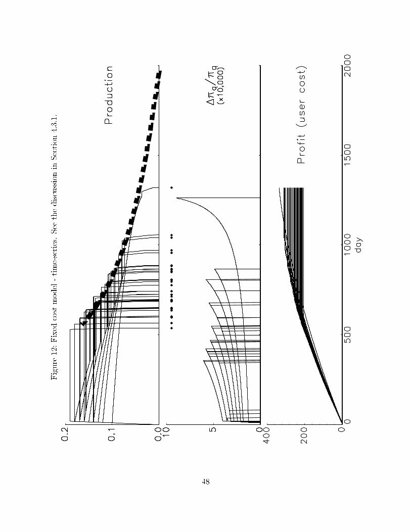
Figure

12:Fixed

cost

model-time-series.See

thediscussionin

Section

4.3.1.

48

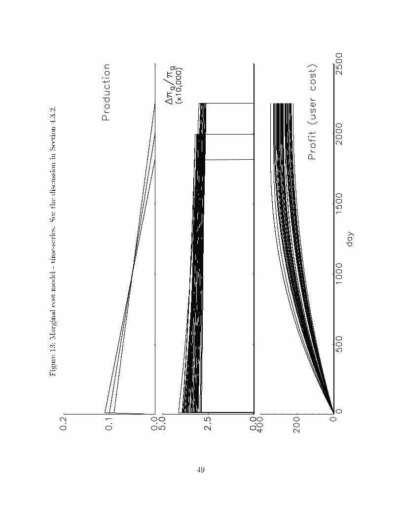
Figure

13:Marginal

cost

model-time-series.See

thediscussionin

Section

4.3.2.

49

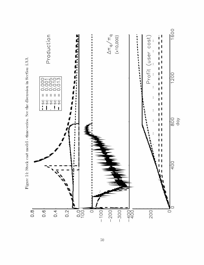
Figure

14:Stock

cost

model-time-series.See

thediscussionin

Section

4.3.3.

50

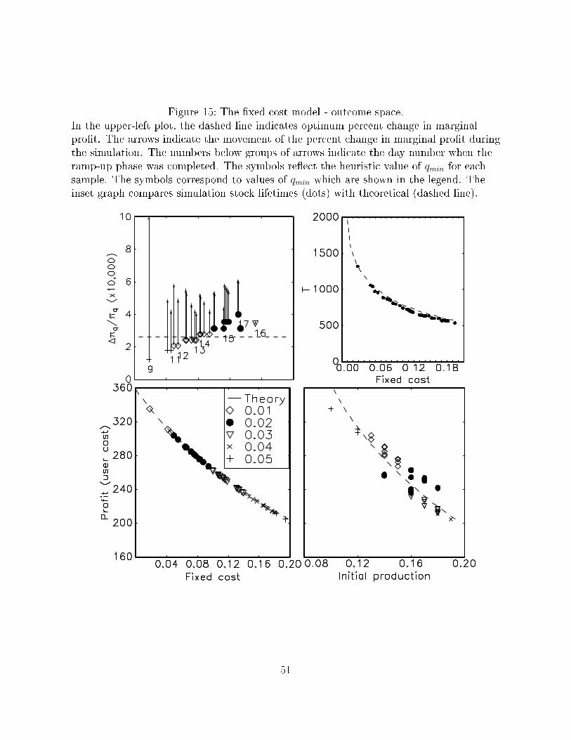
Figure 15: The �xed cost model - outcome space.In the upper-left plot, the dashed line indicates optimum percent change in marginalpro�t. The arrows indicate the movement of the percent change in marginal pro�t duringthe simulation. The numbers below groups of arrows indicate the day number when theramp-up phase was completed. The symbols re�ect the heuristic value of qmin for eachsample. The symbols correspond to values of qmin which are shown in the legend. Theinset graph compares simulation stock lifetimes (dots) with theoretical (dashed line).

51

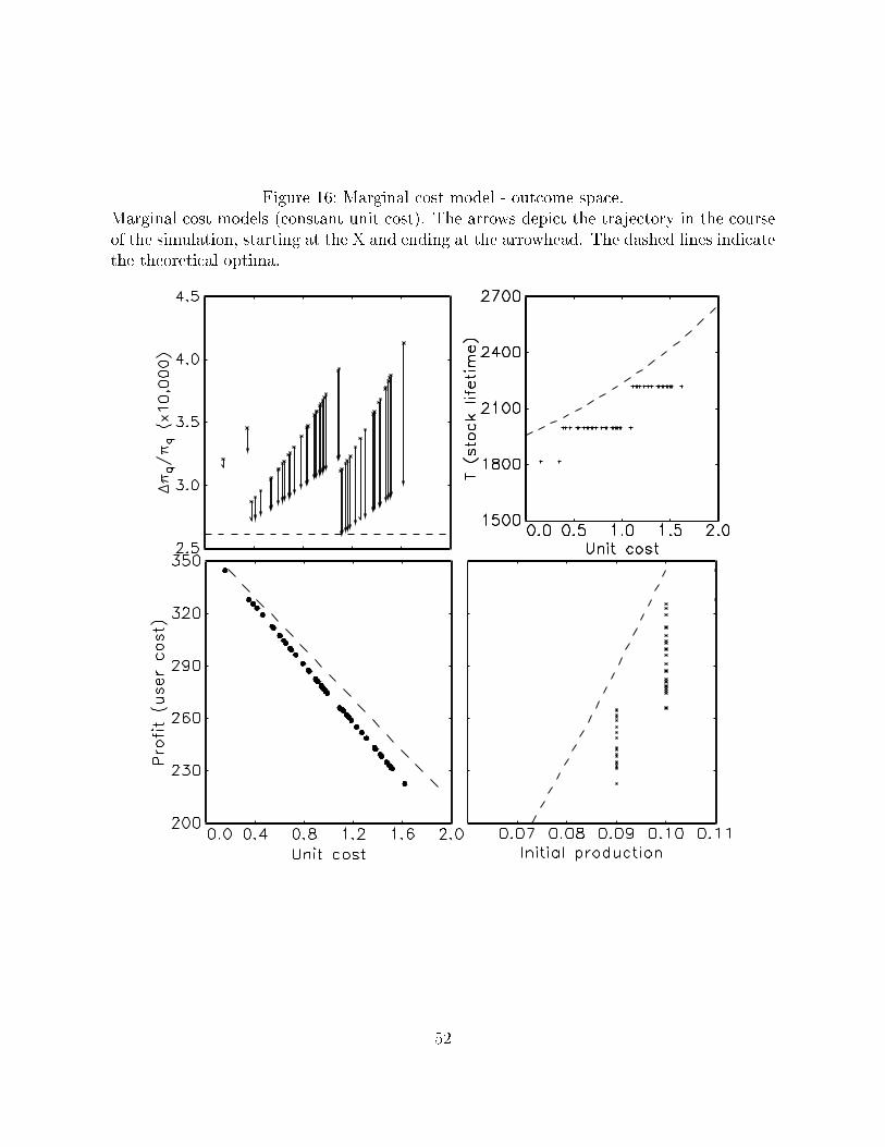
Figure 16: Marginal cost model - outcome space.Marginal cost models (constant unit cost). The arrows depict the trajectory in the courseof the simulation, starting at the X and ending at the arrowhead. The dashed lines indicatethe theoretical optima.

52

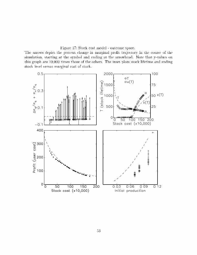
Figure 17: Stock cost model - outcome space.The arrows depict the percent change in marginal pro�t trajectory in the course of thesimulation, starting at the symbol and ending at the arrowhead. Note that y-values onthis graph are 10,000 times those of the others. The inset plots stock lifetime and endingstock level versus marginal cost of stock.

53

change in marginal pro�t can vary over the lifetime of the stock, approaching r percentonly for a costless monopoly. Percent change in marginal pro�t is well above r percent for�xed cost, and greater than or less than r percent for unit and stock costs. These resultsindicate that percent change in marginal pro�t is not a sensitive metric for optimality.A market with even minor ine�ciencies can deviate signi�cantly from the r-percent rule.Conversely, a large deviation from the r-percent rule does not necessarily predict signi�cantine�ciency.The relative e�ectiveness of such a simple heuristic implies that producers may be able

to pro�tably exploit natural resources with very little direct knowledge of the demandfunction or of the market structure. Examined here is pro�tability, but, in principle, theheuristic should perform similarly for a more general social welfare, for instance. That willbe the topic for a forthcoming paper.

54

References

Claudio Agostini. Estimating market power in the US copper industry. Review of IndustrialOrganization, 28(1):17 � 39, 2006. ISSN 0889938X.

K.J. Arrow and S. Chang. Optimal pricing, use, and exploration of uncertain naturalresource stocks. Journal of Environmental Economics and Management, 9(1):1�10, 1982.ISSN 0095-0696.

R. Axelrod. The evolution of strategies in the iterated prisoner's dilemma. Genetic algo-rithms and simulated annealing, pages 32�41, 1987.

R.M. Axelrod. The complexity of cooperation: Agent-based models of competition andcollaboration. Princeton Univ Pr, 1997.

R. Axtell, R. Axelrod, J.M. Epstein, and M.D. Cohen. Aligning simulation models: A casestudy and results. Computational & Mathematical Organization Theory, 1(2):123�141,1996. ISSN 1381-298X.

R.L. Axtell, J.M. Epstein, and H.P. Young. The emergence of classes in a multiagentbargaining model. Social dynamics, pages 191�211, 1999.

H.J. Barnett and C. Morse. Scarcity and growth: The economics of natural resource avail-ability, volume 11. Johns Hopkins University for Resources for the Future, 1963.

Peter Berck and Michael Roberts. Natural resource prices: Will they ever turn up? Journalof Environmental Economics and Management, 31(1):65 � 78, 1996. ISSN 0095-0696.doi: DOI: 10.1006/jeem.1996.0032.

G.M. Brown and B.C. Field. Implications of alternative measures of natural resourcescarcity. The Journal of Political Economy, 86(2):229�243, 1978. ISSN 0022-3808.

R.D. Cairns and N. Van Quyen. Optimal Exploration for and Exploitation of HeterogeneousMineral Deposits. Journal of Environmental Economics and Management, 35(2):164�189, 1998. ISSN 0095-0696.

M.R. Caputo. Foundations of dynamic economic analysis: optimal control theory andapplications. Cambridge Univ Pr, 2005. ISBN 0521603684.

J.M. Chermak and R.H. Patrick. A Microeconometric Test of the Theory of ExhaustibleResources. Journal of Environmental Economics and Management, 42(1):82�103, 2001.

Alpha C. Chiang. Elements of dynamic optimization. McGraw-Hill, 1992. ISBN0070109117.

J.M. Conrad and C.W. Clark. Natural resource economics: notes and problems. CambridgeUniv Pr, 1987. ISBN 0521337690.

55

P. Dasgupta and G.M. Heal. Economic theory and exhaustible resources. Cambridge UnivPr, 1980.

S. Devarajan and A.C. Fisher. Hotelling's "Economics of exhaustible resources": Fiftyyears later. Journal of Economic Literature, 19(1):65�73, 1981.

D.S. Dixon and W.N. Reynolds. The BASP agent-based modeling framework: Applica-tions, scenarios and lessons learned. In System Sciences, 2003. Proceedings of the 36thAnnual Hawaii International Conference on, pages 8�pp. IEEE, 2003. ISBN 0769518745.

J.M. Epstein. Modeling civil violence: An agent-based computational approach. Proceed-ings of the National Academy of Sciences of the United States of America, 99(Suppl 3):7243, 2002.

J.M. Epstein and R. Axtell. Growing arti�cial societies: social science from the bottom up.The MIT Press, 1996. ISBN 0262550253.

Scott Farrow. Testing the e�ciency of extraction from a stock resource. The Journal ofPolitical Economy, 93(3):452�487, 1985. ISSN 00223808.

A.C. Fisher. Resource and environmental economics. Cambridge Univ Pr, 1981. ISBN0521285941.

G. Gaudet and P. Lasserre. On comparing monopoly and competition in exhaustibleresource exploitation. Journal of Environmental Economics and Management, 15(4):412�418, 1988. ISSN 0095-0696.

Gérard Gaudet. Natural resource economics under the rule of Hotelling. Canadian Journalof Economics Revue Canadienne dEconomique, 40:1033�1059, 2007.

G.N. Gilbert and K.G. Troitzsch. Simulation for the social scientist. Open Univ Pr, 2005.

R. Halvorsen and T.R. Smith. On measuring natural resource scarcity. The Journal ofPolitical Economy, 92(5):954�964, 1984. ISSN 0022-3808.

R. Halvorsen and T.R. Smith. A test of the theory of exhaustible resources. The QuarterlyJournal of Economics, 106(1):123, 1991. ISSN 0033-5533.

N. Hanley, J.F. Shogren, B. White, et al. Environmental economics in theory and practice.Macmillan, 1997. ISBN 0333582357.

J.E. Hartley. Retrospectives: The origins of the representative agent. The Journal ofEconomic Perspectives, 10(2):169�177, 1996. ISSN 0895-3309.

G. Heal. The relationship between price and extraction cost for a resource with a backstoptechnology. The Bell Journal of Economics, 7(2):371�378, 1976. ISSN 0361-915X.

56

G. Heal and M. Barrow. The relationship between interest rates and metal price move-ments. The Review of Economic Studies, 47(1):161�181, 1980. ISSN 0034-6527.

Harold Hotelling. The economics of exhaustible resources. Journal of Political Economy,39(2):137�75, 1931.

C.T. Hsiao and L.C. Chang. Dynamic optimal groundwater management with inclusion of�xed costs. Journal of water resources planning and management, 128:57, 2002.

M.I. Kamien and N.L. Schwartz. Dynamic optimization: the calculus of variations andoptimal control in economics and management. North Holland Amsterdam, 1981.

Je�rey A. Krautkraemer. Nonrenewable resource scarcity. Journal of Economic Literature,36(4):2065 � 2107, 1998. ISSN 00220515.

R. Lecomber. Economics of natural resources. MacMillan, London, 1979.

David Levhari and Nissan Liviatan. Notes on Hotelling's economics of exhaustible re-sources. The Canadian Journal of Economics / Revue canadienne d'Economique, 10(2):177�192, 1977. ISSN 00084085.

T.R. Lewis, S.A. Matthews, and H.S. Burness. Monopoly and the rate of extraction ofexhaustible resources: Note. The American Economic Review, 69(1):227�230, 1979.ISSN 0002-8282.

J. Livernois. On the empirical signi�cance of the Hotelling rule. Review of EnvironmentalEconomics and policy, 3(1):22, 2009. ISSN 1750-6816.

J. Livernois and P. Martin. Price, scarcity rent, and a modi�ed r per cent rule for non-renewable resources. Canadian Journal of Economics/Revue canadienne d'économique,34(3):827�845, 2001. ISSN 1540-5982.

J.R. Livernois and R.S. Uhler. Extraction costs and the economics of nonrenewable re-sources. The Journal of Political Economy, 95(1):195�203, 1987. ISSN 0022-3808.

D. McFadzean, D. Stewart, and L. Tesfatsion. A computational laboratory for evolutionarytrade networks. Evolutionary Computation, IEEE Transactions on, 5(5):546�560, 2001.ISSN 1089-778X.

W.D. Nordhaus. The allocation of energy resources. Brookings Papers on Economic Ac-tivity, 1973(3):529�576, 1973.

W.D. Nordhaus. Resources as a Constraint on Growth. The American Economic Review,64(2):22�26, 1974. ISSN 0002-8282.

M.H. Pesaran. An econometric analysis of exploration and extraction of oil in the UKContinental Shelf. The Economic Journal, 100(401):367�390, 1990. ISSN 0013-0133.

57

R.S. Pindyck. The optimal exploration and production of nonrenewable resources. TheJournal of Political Economy, 86(5):841�861, 1978. ISSN 0022-3808.

R.S. Pindyck. On monopoly power in extractive resource markets. Journal of Environ-mental Economics and Management, 14(2):128�142, 1987. ISSN 0095-0696.

LS Pontryagin. Optimal control processes. Uspekhi Mat. Nauk, 14(1):85, 1959.

LS Pontryagin, VG Boltyanski�, RV Gamkrelidze, and EF Mishchenko. The mathematicaltheory of optimal processes, Fizmatgiz, Moscow 1961. English transl., Interscience, NewYork, 1962.

W.N. Reynolds and DS Dixon. Archimedes: A Prototype Distillation. Maneuver WarfareScience, 2001.

J. Rust, J. Miller, and R. Palmer. Behavior of trading automata in a computerized doubleauction market. The double auction market: Institutions, theories, and evidence, pages155�198, 1992.

S.W. Salant. Exhaustible resources and industrial structure: A Nash-Cournot approach tothe world oil market. The Journal of Political Economy, 84(5):1079�1093, 1976. ISSN0022-3808.

T.C. Schelling. Micromotives and Macrobehavior. New York: Norton, 1978.

A.D. Scott. The theory of the mine under conditions of certainty. Extractive Resourcesand Taxation, pages 25�62, 1967.

M.E. Slade. Trends in natural-resource commodity prices: an analysis of the time domain.Journal of Environmental Economics and Management, 9(2):122�137, 1982. ISSN 0095-0696.

M.E. Slade. Tax policy and the supply of exhaustible resources: Theory and practice. LandEconomics, 60(2):133�147, 1984. ISSN 0023-7639.

V.K. Smith. Natural resource scarcity: a statistical analysis. The Review of Economicsand Statistics, 61(3):423�427, 1979. ISSN 0034-6535.

Robert M. Solow. The economics of resources or the resources of economics. The AmericanEconomic Review, 64(2):1�14, 1974. ISSN 00028282.

J.E. Stiglitz. Monopoly and the rate of extraction of exhaustible resources. The AmericanEconomic Review, 66(4):655�661, 1976. ISSN 0002-8282.

Kenneth R. Stollery. Mineral depletion with cost as the extraction limit: A model appliedto the behavior of prices in the nickel industry. Journal of Environmental Economicsand Management, 10(2):151 � 165, 1983. ISSN 0095-0696.

58

J.E. Swierzbinski and R. Mendelsohn. Exploration and exhaustible resources: the micro-foundations of aggregate models. International Economic Review, 30(1):175�186, 1989.ISSN 0020-6598.

L. Tesfatsion. Structure, behavior, and market power in an evolutionary labor marketwith adaptive search. Journal of Economic Dynamics and Control, 25(3-4):419�457,2001. ISSN 0165-1889.

L. Tesfatsion. Agent-based computational economics: A constructive approach to economictheory. Handbook of computational economics, 2:831�880, 2006. ISSN 1574-0021.

T.H. Tietenberg and L. Lewis. Environmental and natural resource economics. Addison-Wesley, 2000. ISBN 0321031288.

H.R. Varian. Microeconomic analysis. 3rd. ed. ed. New York, London: WW Norton &Company, 1992.

D. Young. Cost speci�cation and �rm behaviour in a Hotelling model of resource extraction.Canadian Journal of Economics, 25(1):41�59, 1992.

59