arX

iv:0

802.

0249

v1 [

quan

t-ph

] 2

Feb

200

8

Hopf Algebras in General and in Combinatorial

Physics: a practical introduction

G H E Duchamp†, P Blasiak‡, A Horzela‡, K A Penson♦

and A I Solomon♦,♯

a LIPN - UMR 7030

CNRS - Universite Paris 13

F-93430 Villetaneuse, France

‡ H. Niewodniczanski Institute of Nuclear Physics, Polish Academy of Sciences

ul. Eliasza-Radzikowskiego 152, PL 31342 Krakow, Poland♦ Laboratoire de Physique Theorique des Liquides,

Universite Pierre et Marie Curie, CNRS UMR 7600

Tour 24 - 2e et., 4 pl. Jussieu, F 75252 Paris Cedex 05, France♯ The Open University, Physics and Astronomy Department

Milton Keynes MK7 6AA, United Kingdom

E-mail:

ghed@lipn-univ.paris13.fr, pawel.blasiak@ifj.edu.pl,

andrzej.horzela@ifj.edu.pl, penson@lptl.jussieu.fr,

a.i.solomon@open.ac.uk

Abstract. This tutorial is intended to give an accessible introduction to Hopf

algebras. The mathematical context is that of representation theory, and we also

illustrate the structures with examples taken from combinatorics and quantum physics,

showing that in this latter case the axioms of Hopf algebra arise naturally. The

text contains many exercises, some taken from physics, aimed at expanding and

exemplifying the concepts introduced.

1. Introduction

Quantum Theory seen in action is an interplay of mathematical ideas and physical

concepts. From a modern perspective its formalism and structure are founded on the

theory of Hilbert spaces [36, 44]. Using a few basic postulates, the physical notions of a

system and apparatus, as well as transformations and measurements, are described in

terms of linear operators. In this way the algebra of operators constitutes a proper

mathematical framework within which quantum theories may be constructed. The

structure of this algebra is determined by two operations, namely - addition and

multiplication of operators; and these lie at the root of all fundamental aspects of

Quantum Theory.

Version 23 October 2018

1

The formalism of quantum theory represents the physical concepts of states, observables

and their transformations as objects in some Hilbert space H and subsequently provides

a scheme for measurement predictions. Briefly, vectors in the Hilbert space describe

states of a system, and linear forms in V∗ represent basic observables. Both concepts

combine in the measurement process which provides a probabilistic distribution of

results and is given by the Born rule. Physical information about the system is

gained by transforming the system and/or apparatus in various ways and performing

measurements. Sets of transformations usually possess some structure – such as that

of a group, semi-group, Lie algebra, etc. – and in general can be handled within the

concept of an algebra A. The action of the algebra on the vector space of states V and

observables V∗ is simply its representation. Hence if an algebra is to describe physical

transformations it has to have representations in all physically relevant systems. This

requirement directly leads to the Hopf algebra structures in physics.

From the mathematical viewpoint the structure of the theory, modulo details, seems to

be clear. Physicists, however, need to have some additional properties and constructions

to move freely in this arena. Here we will show how the structure of Hopf algebras

enters into the game in the context of representations. The first issue at point is the

construction of tensor product of vector spaces which is needed for the description of

composite systems. Suppose, we know how some transformations act on individual

systems, i.e. we know representations of the algebra in each vector space V1 and

V2, respectively. Hence natural need arises for a canonical construction of an induced

representation of this algebra in V1⊗V2 which would describe its action on the composite

system. Such a scheme exists and is provided by the co-product in the algebra, i.e. a

morphism ∆ : A −→ A ⊗ A. The physical plausibility of this construction requires

the equivalence of representations built on (V1 ⊗ V2) ⊗ V3 and V1 ⊗ (V2 ⊗ V3) – since

the composition of three systems can not depend on the order in which it is done.

This requirement forces the co-product to be co-associative. Another point is connected

with the fact that from the physical point of view the vector space C represents a

trivial system having only one property – “being itself” – which can not change.

Hence one should have a canonical representation of the algebra on a trivial system,

denoted by ǫ : A −→ C. Next, since the composition of any system with a trivial one

can not introduce new representations, those on V and V ⊗ C should be equivalent.

This requirement imposes the condition on ǫ to be a co-unit in the algebra. In this

way we motivate the need for a bi-algebra structure in physics. The concept of an

antipode enters in the context of measurement. Measurement in a system is described

in in terms of V∗ × V and measurement predictions are given through the canonical

pairing c : V∗ × V −→ C. Observables, described in the dual space V∗, can also be

transformed and representations of appropriate algebras are given with the help of an

anti-morphism α : A −→ A. Physics requires that transformation preformed on the

system and apparatus simultaneously should not change the measurement results, hence

the pairing should trivially transform under the action of the bi-algebra. We thus obtain

the condition on α to be an antipode, which is the last ingredient of a Hopf Algebra.

2

Many Hopf algebras are motivated by various theories (physical or close to physics)

such as renormalization [12, 11, 14, 16, 40], non-commutative geometry [16, 17], physical

chemistry [43, 13], computer science [29], algebraic combinatorics [14, 30, 41, 19], algebra

[31, 32, 33].

2. Operators

2.1. Generalities

Throughout this text we will consider (linear) operators ω : V −→ V , where V is a

vector space over k (k is a field of scalars which can be thought of as R or C). The set

of all (linear) operators V −→ V is an algebra (see appendix) which will be denoted by

EndK(V ).

2.2. What is a representation

It is not rare in Physics that we consider, instead of a single operator, a set or a family

of operators (ωα)α∈A and often the index set itself has a structure. In the old books one

finds the family-like notation, where ρ(α) is denoted, say, ωα. As a family of operators

(ωα)α∈A is no more than a mapping ρ : A 7→ Endk(V ) (see [6], Ch. II 3.4 remark), we

wprefer to exhibit the mapping by considering it defined as such. This will be precisely

the concept of representation that we will illustrate by familiar examples. Moreover

using arrows allows, as we will see more clearly below, for extension and factorization

procedures.

• First case: A is a group

In this case, we postulate that the action of the operators be compatible with the laws

of a group; that is, for all α, β ∈ A,

{

ρ(α.β) = ρ(α) ◦ ρ(β)ρ(α−1) = (ρ(α))−1 (1)

which is equivalent to

{

ρ(α.β) = ρ(α) ◦ ρ(β)ρ(1A) = 1End(V )

(2)

Note that each of these conditions implies that the range of ρ is in Autk(V ) (= GLn(k),

the linear group), the set of one-to-one elements of Endk(V ) (called automorphisms).

• Second case: A is a Lie algebra

3

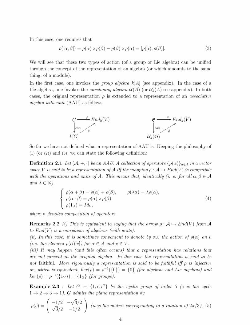
In this case, one requires that

ρ([α, β]) = ρ(α) ◦ ρ(β)− ρ(β) ◦ ρ(α) = [ρ(α), ρ(β)]. (3)

We will see that these two types of action (of a group or Lie algebra) can be unified

through the concept of the representation of an algebra (or which amounts to the same

thing, of a module).

In the first case, one invokes the group algebra k[A] (see appendix). In the case of a

Lie algebra, one invokes the enveloping algebra U(A) (or Uk(A) see appendix). In both

cases, the original representation ρ is extended to a representation of an associative

algebra with unit (AAU) as follows:

Gρ //

can

��

Endk(V )

k[G]

ρ

99ttttttttt

Gρ //

can

��

Endk(V )

Uk(G)

ρ

99ssssssssss

So far we have not defined what a representation of AAU is. Keeping the philosophy of

(1) (or (2)) and (3), we can state the following definition:

Definition 2.1 Let (A,+, ·) be an AAU. A collection of operators {ρ(α)}α∈A in a vector

space V is said to be a representation of A iff the mapping ρ : A 7→ End(V ) is compatible

with the operations and units of A. This means that, identically (i. e. for all α, β ∈ Aand λ ∈ K).

ρ(α + β) = ρ(α) + ρ(β), ρ(λα) = λρ(α),

ρ(α · β) = ρ(α) ◦ ρ(β),ρ(1A) = IdV ,

(4)

where ◦ denotes composition of operators.

Remarks 2.2 (i) This is equivalent to saying that the arrow ρ : A 7→ End(V ) from Ato End(V ) is a morphism of algebras (with units).

(ii) In this case, it is sometimes convenient to denote by α.v the action of ρ(α) on v

(i.e. the element ρ(α)[v]) for α ∈ A and v ∈ V .

(iii) It may happen (and this often occurs) that a representation has relations that

are not present in the original algebra. In this case the representation is said to be

not faithful. More rigourously a representation is said to be faithful iff ρ is injective

or, which is equivalent, ker(ρ) = ρ−1({0}) = {0} (for algebras and Lie algebras) and

ker(ρ) = ρ−1({1V }) = {1G} (for groups).

Example 2.3 : Let G = {1, c, c2} be the cyclic group of order 3 (c is the cycle

1→ 2→ 3→ 1), G admits the plane representation by

ρ(c) =

(

−1/2 −√3/2√

3/2 −1/2

)

(it is the matrix corresponding to a rotation of 2π/3). (5)

4

Thus,

ρ(c2) =

(

−1/2√3/2

−√3/2 −1/2

)

and, of course, ρ(1) =

(

1 0

0 1

)

. (6)

The representation ρ is faithful while its extension to the group algebra is not, as seen

from:

ρ(1 + c+ c2) =

(

0 0

0 0

)

whereas 1 + c + c2 6= 0 in C[G]. (7)

Note 2.4 Note that the situation is even worse for a Lie algebra, as Uk(G) is infinite

dimensional iff G is not zero.

3. Operations on representations

Now, we would like to see the representations of AAU as building blocks to construct

new ones. The elementary operations on vector spaces are:

- sums

- tensor products

- duals

Hence, an important problem is:

Given representations ρi : A 7→ Vi on the building blocks Vi ; i = 1, 2 how does one

naturally construct representations on V1 ⊕ V2, V1 ⊗ V2 and V ∗i .

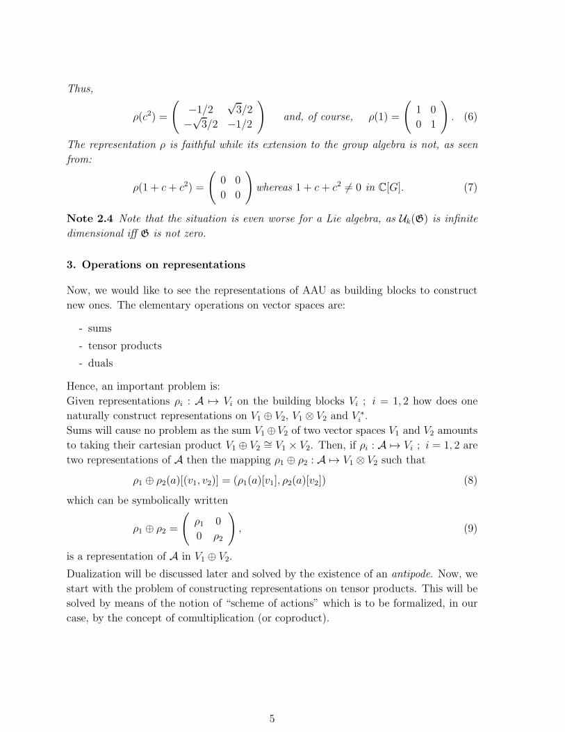
Sums will cause no problem as the sum V1⊕V2 of two vector spaces V1 and V2 amounts

to taking their cartesian product V1 ⊕ V2 ∼= V1 × V2. Then, if ρi : A 7→ Vi ; i = 1, 2 are

two representations of A then the mapping ρ1 ⊕ ρ2 : A 7→ V1 ⊗ V2 such that

ρ1 ⊕ ρ2(a)[(v1, v2)] = (ρ1(a)[v1], ρ2(a)[v2]) (8)

which can be symbolically written

ρ1 ⊕ ρ2 =(

ρ1 0

0 ρ2

)

, (9)

is a representation of A in V1 ⊕ V2.Dualization will be discussed later and solved by the existence of an antipode. Now, we

start with the problem of constructing representations on tensor products. This will be

solved by means of the notion of “scheme of actions” which is to be formalized, in our

case, by the concept of comultiplication (or coproduct).

5

3.1. Arrows and addition or multiplication formulas

Let us give first some examples where comultiplication naturally arises.

We begin with functions admitting an “addition formula” or “multiplication formula”.

This means functions such that for all x, y

f(x ∗ y) =n∑

i=1

f(1)i (x)f

(2)i (y), (10)

where ∗ is a certain (associative) operation on the defining set of f and (f(1)i , f

(2)i )ni=1

be two (finite) families of functions on the same set (see exercises (11.1) and (11.2) on

representative functions).

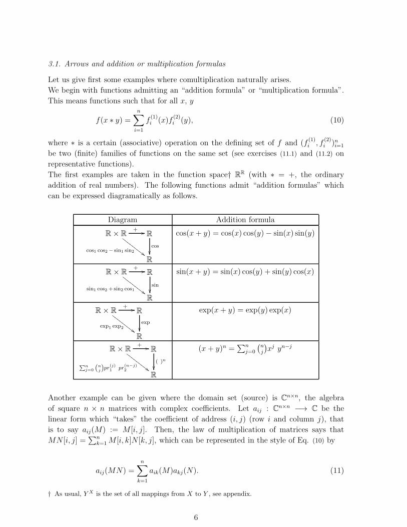
The first examples are taken in the function space† RR (with ∗ = +, the ordinary

addition of real numbers). The following functions admit “addition formulas” which

can be expressed diagramatically as follows.

Diagram Addition formula

R× R+ //

cos1 cos2 − sin1 sin2 ##FFFF

FFFF

FR

cos

��R

cos(x+ y) = cos(x) cos(y)− sin(x) sin(y)

R× R+ //

sin1 cos2 +sin2 cos1 ##FFFF

FFFF

FR

sin��R

sin(x+ y) = sin(x) cos(y) + sin(y) cos(x)

R× R+ //

exp1 exp2 ##FFFF

FFFF

FR

exp

��R

exp(x+ y) = exp(y) exp(x)

R× R+ //

Pnj=0 (

n

j)pr(j)1 pr

(n−j)2 ##FF

FFFF

FFF

R

( )n

��R

(x+ y)n =∑n

j=0

(

nj

)

xj yn−j

Another example can be given where the domain set (source) is Cn×n, the algebra

of square n × n matrices with complex coefficients. Let aij : Cn×n −→ C be the

linear form which “takes” the coefficient of address (i, j) (row i and column j), that

is to say aij(M) := M [i, j]. Then, the law of multiplication of matrices says that

MN [i, j] =∑n

k=1M [i, k]N [k, j], which can be represented in the style of Eq. (10) by

aij(MN) =n∑

k=1

aik(M)akj(N). (11)

† As usual, Y X is the set of all mappings from X to Y , see appendix.

6

Cn×n × Cn×nproduct //

Pnk=1(aik)1(akj )2

))SSSSSSSSSSSSSSSSSCn×n

aij

��C

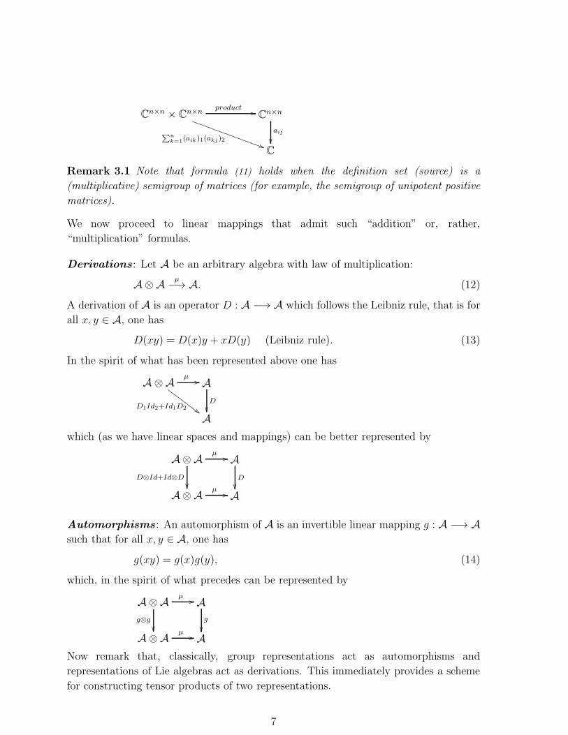
Remark 3.1 Note that formula (11) holds when the definition set (source) is a

(multiplicative) semigroup of matrices (for example, the semigroup of unipotent positive

matrices).

We now proceed to linear mappings that admit such “addition” or, rather,

“multiplication” formulas.

Derivations : Let A be an arbitrary algebra with law of multiplication:

A⊗A µ−→ A. (12)

A derivation of A is an operator D : A −→ A which follows the Leibniz rule, that is for

all x, y ∈ A, one has

D(xy) = D(x)y + xD(y) (Leibniz rule). (13)

In the spirit of what has been represented above one has

A⊗A µ //

D1Id2+Id1D2 ##GGGG

GGGG

GAD

��A

which (as we have linear spaces and mappings) can be better represented by

A⊗A µ //

D⊗Id+Id⊗D��

AD

��A⊗A µ // A

Automorphisms : An automorphism of A is an invertible linear mapping g : A −→ Asuch that for all x, y ∈ A, one has

g(xy) = g(x)g(y), (14)

which, in the spirit of what precedes can be represented by

A⊗A µ //

g⊗g

��

Ag

��A⊗A µ // A

Now remark that, classically, group representations act as automorphisms and

representations of Lie algebras act as derivations. This immediately provides a scheme

for constructing tensor products of two representations.

7

Tensor product of two representations (groups and Lie algebras): First, take

two representations of a group G, ρi : G −→ End(Vi), i = 1, 2. The action of g ∈ G on

the tensor space V1 ⊗ V2 is given by

g(v1 ⊗ v2) = g(v1)⊗ g(v2). (15)

This means that the “tensor product” of the two (group) representations ρi, i = 1, 2 is

given by the following data

• Space : V1 ⊗ V2• Action : ρ1×ρ2 : g → ρ1(g)⊗ ρ2(g)

Likewise, if we have two representations ρi : G −→ End(Vi), i = 1, 2 of the Lie algebra

G the action of g ∈ G on a tensor product V1 ⊗ V2 is given by

g(v1 ⊗ v2) = g(v1)⊗ v2 + v1 ⊗ g(v2). (16)

Again, the “tensor product” of the two (Lie algebra) representations ρi, i = 1, 2 is given

by the following data

• Space : V1 ⊗ V2• Action : ρ1×ρ2 : g → ρ1(g)⊗ IdV2(g) + IdV1(g)⊗ ρ2(g)

Roughly speaking, in the first case g acts by g⊗g and in the second one by g⊗1+1⊗g.In view of two above cases it is convenient to construct linear mappings:

A ∆−→ A⊗A , (17)

such that, in each case, ρ1×ρ2 = (ρ1 ⊗ ρ2) ◦∆.

In the first case (A = C[G]) one gets

∆

(

∑

g∈G

αgg

)

=∑

g∈G

αgg ⊗ g. (18)

In the second case, one has first to construct the comultiplication on the monomials

g1...gn; gi ∈ G) as they span (A = Uk(G)). Then, using the rule ∆(g) = g⊗1+1⊗g (forg ∈ G) and the fact that ∆ is supposed to be a morphism for the multiplication (the

justification of this rests on the fact that the constructed action must be a representation

see below around formula (36) and exercise (11.5)), one has

∆(g1...gn) = (g1 ⊗ 1 + 1⊗ g1)(g2 ⊗ 1 + 1⊗ g2)...(gn ⊗ 1 + 1⊗ gn)=

∑

I+J=[1...n]

g[I]⊗ g[J ]. (19)

Where, for I = {i1, i2, · · · , ik} (1 ≤ i1 < i2 < · · · < ik ≤ n), g[I] stands for

gi1gi2 · · · gik In each case (group algebra and envelopping algebra) one again gets a

mapping ∆ : A 7→ A⊗A which will be expressed by

∆(a) =n∑

i=1

a(1)i ⊗ a

(2)i (20)

8

which is rephrased compactly by

∆(a) =∑

(1)(2)

a(1) ⊗ a(2). (21)

The action of a ∈ A on a tensor v1 ⊗ v2 is then, in both cases, given by

a.(v1 ⊗ v2) =n∑

i=1

a(1)i .v1 ⊗ a(2)i .v2 =

∑

(1)(2)

a(1).v1 ⊗ a(2).v2. (22)

One can easily check, in these two cases, that

a.b.(v1 ⊗ v2) = (ab).(v1 ⊗ v2), (23)

but in general (22) does not guarantee (23); this point will be discussed below in section

(4).

Expression (21) is very convenient for proofs and computations and known as Sweedler’s

notation.

Remarks 3.2 i) In every case, we have extracted the “scheme of action” for building the

tensor product of two representations. This scheme (a linear mapping ∆ : A 7→ A⊗A)is independent of the considered representations and, in each case,

ρ1×ρ2 = (ρ1 ⊗ ρ2) ◦∆ (24)

ii) Sweedler’s notation becomes transparent when one speaks the language of “structure

constants”. Let ∆ : C 7→ C ⊗ C be a comultiplication and (bi)i∈I a (linear) basis of C.One has

∆(bi) =∑

j,k∈I

λj,ki bj ⊗ bk . (25)

the family (λj,ki )i,j,k∈I is called the “structure constants” of the comultiplication ∆. Note

the duality with the notion the “structure constants” of a multiplication

µ : A⊗A 7→ A : if (bi)i∈I is a (linear) basis of A, one has

µ(bi ⊗ bj) =∑

k∈I

λki,j bk . (26)

For necessary and sufficient conditions for a family to be structure constants (see exercise

(11.12)).

Then, the general construction for tensor products goes as follows.

Definition 3.3 : Let A be a vector space, a comultiplication ∆ on A is a linear mapping

A ∆−→ A⊗A.

Such a pair (vector space, comultiplication) without any prescription about the linear

mapping “comultiplication” is called a coalgebra.

9

Now, imitating (24), if A is an algebra and ρ1, ρ2 are representations of A in V1, V2, for

each a ∈ A, we can construct an action of a on V1 ⊗ V2 by

V1 ⊗ V2(ρ1⊗ρ2)◦∆(a)−→ V1 ⊗ V2. (27)

This means that if ∆(a) =∑

(1)(2) a(1) ⊗ a(2), then, (a) acts on the tensor product by

a.(v1 ⊗ v2) =∑

(1)(2)

a(1).v1 ⊗ a(2).v2 =∑

(1)(2)

ρ1(a(1))[v1]⊗ ρ2(a(2))[v2]. (28)

But, at this stage, it is just an action and not (necessarily) a representation of A. We

shall later give the requirements on ∆ for the construction of the tensor product to be

reasonable (i. e. compatible with the usual tensor properties).

For the moment let us pause and consider some well known examples of comultiplication.

3.2. Combinatorics of some comultiplications

The first type of comultiplication is given by duality. This means by a formula of type

〈∆(x)|y ⊗ z〉⊗2 = 〈x|y ∗ z〉 (29)

for a certain law of algebra V ⊗ V ∗7→ V , where 〈 | 〉 is a non degenerate scalar product

in V and 〈 | 〉⊗2 stands for its extension to V ⊗ V . In the case of words ∗ is the

concatenation and 〈 | 〉 is given by 〈u|v〉 = δu,v. The comultiplication ∆Cauchy, dual to

the concatenation, is given on a word w by

∆(w) =∑

uv=w

u⊗ v. (30)

In the same spirit, one can define a comultiplication on the algebra of a finite group by

∆(g) =∑

g1g2=g

g1 ⊗ g2. (31)

The second example is given by the multiplication law of elementary comultiplications,

that is, if for each letter x one has ∆(x) = x⊗ 1 + 1⊗ x, then∆(w) = ∆(a1...an) = ∆(a1)∆(a2)...∆(an)

=∑

I+J=[1...n]

w[I]⊗ w[J ] (32)

where w[{i1, i2, · · · ik}] = ai1ai2 · · · aik (for 1 ≤ i1 < i2 < · · · < ik ≤ n). This

comultiplication is dual to (34) below for q = 0 (shuffle product).

Another example is a deformation (perturbation for small q) of the preceding. With

∆(a) = a⊗ 1 + 1⊗ a+ qa⊗ a, one has

∆(w) = ∆(a1...an) = ∆(a1)∆(a2)...∆(an)

=∑

I∪J=[1...n]

q|I∩J |w[I]⊗ w[J ]. (33)

Note that this comultiplication is dual (in the sense of (29)) to the q-infiltration product

given by the recursive formula (for general q and with 1A∗ as the empty word)

10

w ↑ 1A∗ = 1A∗ ↑ w = w

au ↑ bv = a(u ↑ bv) + b(au ↑ v) + qδa,b(u ↑ v). (34)

This product is an interpolation between the shuffle (q = 0) and the (classical)

infiltration (q = 1) [22].

4. Requirements for a reasonable construction of tensor products

We have so far constructed an action of A on tensors, but nothing indicates that this is

a representation (see exercise (11.5)). So, the following question is natural.

Q.1.) If A is an algebra and ∆ : A 7→ A⊗A, what do we require on ∆ if we want the

construction above to be a representation of A on tensor products ?

For a, b ∈ A, ρi representations of A in Vi, and vi ∈ Vi for i = 1, 2, we must have the

following identity:

a.(b.v1 ⊗ v2) = (ab).v1 ⊗ v2 ⇐⇒ ∆(ab).v1 ⊗ v2 = ∆(a).(∆(b).v1 ⊗ v2). (35)

One can prove that, if this is true identically for all a, b ∈ A and all pairs of

representations (see exercise (11.5)), one has

∆(ab) = ∆(a)∆(b). (36)

and, of course, if the latter holds, (35) is true.

This can be rephrased by saying that ∆ is a morphism A 7→ A⊗A.Now, one would like to keep compatibility with the associativity of tensor products.

This means that if we want to tensor u ⊗ v with w it must give the same action as

tensoring u with v ⊗ w. This means that we have to address the following question.

Q.2.) If A is an algebra and ∆ : A 7→ A ⊗ A is a morphism of algebras, what do we

require on ∆ if we want the construction above to be associative ?

More precisely, for three representations ρi, i = 1, 2, 3 of A, we want

ρ1×(ρ2×ρ3) = (ρ1×ρ2)×ρ3 (37)

up to the identifications (u⊗ v)⊗ w = u ⊗ (v ⊗ w) = u ⊗ v ⊗ w (if one is not satisfied

with this identification, see exercise (11.6)).

Let us compute (up to the identification above)

a.[(u⊗ v)⊗ w] = ∆(a).(u⊗ v)⊗ w =(

(∆⊗ Id) ◦∆(a))(

u⊗ v ⊗ w)

(38)

on the other hand

a.[u⊗ (v ⊗ w)] = ∆(a).u⊗ (v ⊗ w) =(

(Id⊗∆) ◦∆(a))(

u⊗ v ⊗ w)

. (39)

11

Again, one can prove (see exercise (11.6)) that this holds identically (i. e. for every

a ∈ A and triple of representations) iff (Id⊗∆) ◦∆ = (∆⊗ Id) ◦∆, i.e.

A ∆ //

∆��

A⊗AId⊗∆

��A⊗A ∆⊗Id // A⊗A⊗A

(40)

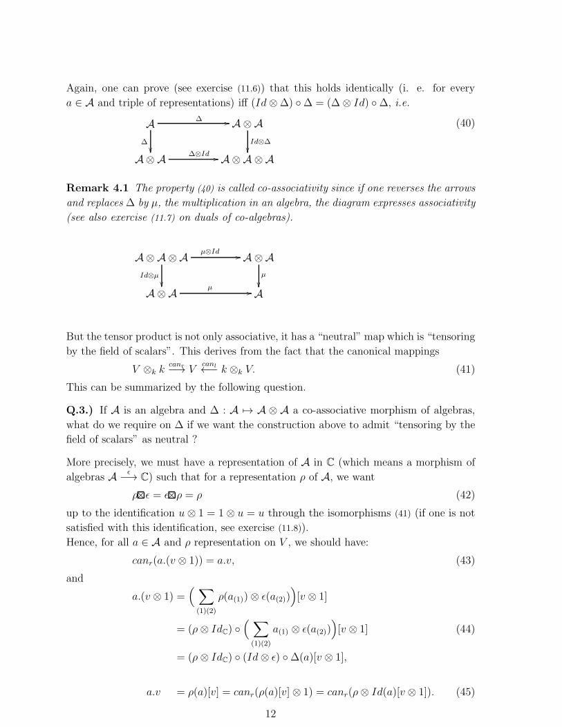
Remark 4.1 The property (40) is called co-associativity since if one reverses the arrows

and replaces ∆ by µ, the multiplication in an algebra, the diagram expresses associativity

(see also exercise (11.7) on duals of co-algebras).

A⊗A⊗A µ⊗Id //

Id⊗µ��

A⊗Aµ

��A⊗A µ // A

But the tensor product is not only associative, it has a “neutral” map which is “tensoring

by the field of scalars”. This derives from the fact that the canonical mappings

V ⊗k kcanr−→ V

canl←− k ⊗k V. (41)

This can be summarized by the following question.

Q.3.) If A is an algebra and ∆ : A 7→ A ⊗ A a co-associative morphism of algebras,

what do we require on ∆ if we want the construction above to admit “tensoring by the

field of scalars” as neutral ?

More precisely, we must have a representation of A in C (which means a morphism of

algebras A ǫ−→ C) such that for a representation ρ of A, we want

ρ×ǫ = ǫ×ρ = ρ (42)

up to the identification u⊗ 1 = 1 ⊗ u = u through the isomorphisms (41) (if one is not

satisfied with this identification, see exercise (11.8)).

Hence, for all a ∈ A and ρ representation on V , we should have:

canr(a.(v ⊗ 1)) = a.v, (43)

and

a.(v ⊗ 1) =(

∑

(1)(2)

ρ(a(1))⊗ ǫ(a(2)))

[v ⊗ 1]

= (ρ⊗ IdC) ◦(

∑

(1)(2)

a(1) ⊗ ǫ(a(2)))

[v ⊗ 1] (44)

= (ρ⊗ IdC) ◦ (Id⊗ ǫ) ◦∆(a)[v ⊗ 1],

a.v = ρ(a)[v] = canr(ρ(a)[v]⊗ 1) = canr(ρ⊗ Id(a)[v ⊗ 1]). (45)

12

Similar computations could be made on the left, we leave them to the reader as an

exercise.

This means that one should require that

A ∆ //

Id��

A⊗AId⊗ǫ

��A A⊗ C

canroo

A ∆ //

Id��

A⊗Aǫ⊗Id

��A C⊗Acanloo

Such a mapping ǫ : A −→ C is called a co-unit.

Remark 4.2 Again, one can prove (see excercice (11.7) for details) that

ǫ is a counit for (A,∆) ⇐⇒ ǫ is a counit for (A∗, ∗∆). (46)

5. Bialgebras

Motivated by the preceding discussion, we define a bialgebra an algebra (associative with

unit) endowed with a comultiplication (co-associative with counit) which allows for the

two tensor properties of associativity and unit (see discussion above). More precisely

Definition 5.1 : (A, ·, 1A,∆, ǫ) is said to be a bialgebra iff

(1) (A, ·, 1A) is an AAU,

(2) (A,∆, ǫ) is a coalgebra coassociative with counit,

(3) ∆ is a morphism of AAU and ǫ is a morphism of AAU.

The name bialgebra comes from the fact that the space A is endowed with two structures

(one of AAU and one of co-AAU) with a certain compatibility between the two.

5.1. Examples of bialgebras

Free algebra (word version : noncommutative polynomials)

Let A be an alphabet (a set of variables) and A∗ be the free monoid constructed on A

(see Basic Structures (12.2)). For any field of scalars k (one may think of k = R or C),

we call the algebra of noncommutative polynomials k〈A〉 (or free algebra), the algebra

k[A∗] of the free monoid A∗ constructed on A. This is the set of functions f : A∗ 7→ k

with finite support endowed with the convolution product

f ∗ g(w) =∑

uv=w

f(u)g(v) (47)

Each word w ∈ A∗ is identified with its characteristic function (i.e. the Dirac function

with value 1 at w and 0 elsewhere). These functions form a basis of k〈A〉 and then,

every f ∈ k〈A〉 can be written uniquely as a finite sum f =∑

f(w)w.

The inclusion mapping A → k〈A〉 will be denoted here by canA.

Comultiplications The free algebra k〈A〉 admits many comultiplications (even with

the two requirements of being a morphism and coassociative). As A∗ is a basis of k〈A〉,

13

it is sufficient to define it on the words (if we require ∆ to be a morphism it is enough

to define it on letters).

Example 1 . — The first example is the dual of the Cauchy (or convolution) product

∆(w) =∑

uv=w

u⊗ v (48)

is not a morphism as

∆(ab) = ab⊗ 1 + a⊗ b+ 1⊗ aband

∆(a)∆(b) = ab⊗ 1 + a⊗ b+ b⊗ a + 1⊗ abbut it can be checked that it is coassociative (see also exercice (11.7) for a quick proof

of this fact).

Example 2 . — A second example is given, on the alphabet A = {a, b} by

∆(a) = a⊗ b; ∆(b) = b⊗ a

then ∆(w) = w⊗ w where w stands for the word w with a (resp. b) changed in b (resp.

a). This comultiplication is a morphism but not coassociative as

(I ⊗∆) ◦∆(a) = a⊗ b⊗ a ; (∆⊗ I) ◦∆(a) = a⊗ a⊗ b

Example 3 . — The third example is given on the letters by

∆(a) = a⊗ 1 + 1⊗ a+ qa⊗ a

where q ∈ k. One can prove that

∆(w) = ∆(a1...an) = ∆(a1)∆(a2)...∆(an) =∑

I∪J=[1..|w|]

q|I∩J |w[I]⊗ w[J ] (49)

this comultiplication is coassociative.

For q = 0, one gets a comultiplication given on the letters by ∆s(a) = a ⊗ 1 + 1 ⊗ a.For every polynomial P ∈ k〈A〉, set ǫ(P ) = P (1A∗) (the constant term). Then

(k〈A〉, ∗,∆s, ǫ) is a bialgebra.

One has also another bialgebra structure with, for all a ∈ A∆h(a) = a⊗ a ; ǫaug(a) = 1 (50)

this bialgebra (k〈A〉, ∗,∆h, ǫaug) is a substructure of the bialgebra of the free group.

Algebra of polynomials (commutative polynomials)

We continue with the same alphabet A, but this time, we take as algebra k[A]. The

construction is similar but the monomials, instead of words, are all the commutative

products of letters i.e. aα11 a

α22 · · ·aαn

n with n arbitrary and αi ∈ N. Denoting MON(A)

the monoid of these monomials (comprising, as neutral, the empty one) and with

∆s(a) = a ⊗ 1 + 1 ⊗ a, ǫ(P ) = P (1MON(A)), one can again check that (k[A], ∗,∆s, ǫ) is

a bialgebra.

14

Algebra of partially commutative polynomials

For the detailed construction of a partially commutative monoid, the reader is referred

to [18, 23]. These monoids generalize both the free and free commutative monoids. To a

given graph (non-oriented and without loops) ϑ ⊂ A×A, one can asssociate the monoid

presented by generators and relations (see basic structures (12.2) and diagram (137))

M(A, ϑ) = 〈A; (xy = yx)(x,y)∈ϑ〉Mon . (51)

This is exactly the monoid obtained as a quotient structure of the free monoid (A∗) by

the smallest equivalence compatible with products (a congruence‡) which contains the

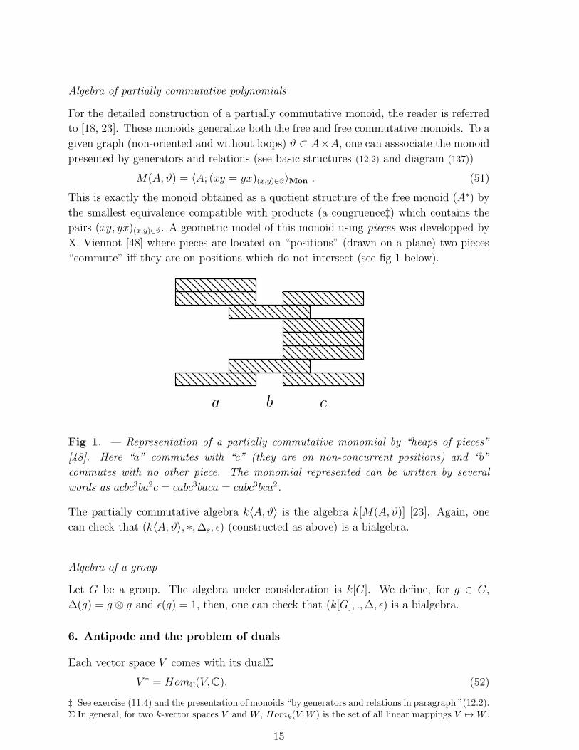
pairs (xy, yx)(x,y)∈ϑ. A geometric model of this monoid using pieces was developped by

X. Viennot [48] where pieces are located on “positions” (drawn on a plane) two pieces

“commute” iff they are on positions which do not intersect (see fig 1 below).

a b c

Fig 1. — Representation of a partially commutative monomial by “heaps of pieces”

[48]. Here “a” commutes with “c” (they are on non-concurrent positions) and “b”

commutes with no other piece. The monomial represented can be written by several

words as acbc3ba2c = cabc3baca = cabc3bca2.

The partially commutative algebra k〈A, ϑ〉 is the algebra k[M(A, ϑ)] [23]. Again, one

can check that (k〈A, ϑ〉, ∗,∆s, ǫ) (constructed as above) is a bialgebra.

Algebra of a group

Let G be a group. The algebra under consideration is k[G]. We define, for g ∈ G,

∆(g) = g ⊗ g and ǫ(g) = 1, then, one can check that (k[G], .,∆, ǫ) is a bialgebra.

6. Antipode and the problem of duals

Each vector space V comes with its dualΣ

V ∗ = HomC(V,C). (52)

‡ See exercise (11.4) and the presentation of monoids “by generators and relations in paragraph ”(12.2).Σ In general, for two k-vector spaces V and W , Homk(V,W ) is the set of all linear mappings V 7→W .

15

The spaces V ∗ and V are in duality by

〈p, ψ〉 = p(ψ) (53)

Now, if one has a representation (on the left) of A on V , one gets a representation on

the right on V ∗ by

〈p.a, ψ〉 = 〈p, a.ψ〉 (54)

If we want to have the action of A on the left again, one should use an anti-morphism

α : A −→ A that is α ∈ Endk(A) such that, for all x, y ∈ Aα(xy) = α(y)α(x). (55)

In the case of groups, g −→ g−1 does the job; in the case of Lie algebras g −→ −g(extended by reverse products to the enveloping algebra) works.

On the other hand, in the classical textbooks, the discussion of “complete reductibility”

goes with the existence of an “invariant” scalar product φ : V × V 7→ k on a space V .

For a group G, this reads

(∀g ∈ G)(∀x, y ∈ V )(

φ(g.x, g.y) = φ(x, y))

(56)

(think of unitary representations).

For a Lie algebra G, this reads

(∀g ∈ G)(∀x, y ∈ V )(

φ(g.x, y) + φ(x, g.y) = 0)

(57)

(think of the Killing form).

Now, linearizing the situation by Φ(x ⊗ y) = φ(x, y) and remembering our unit

representation, one can rephrase (56) and (57) in

(∀a ∈ A)(∀x, y ∈ V )(

Φ(∑

(1)(2)

a(1).x⊗ a(2).y) = ǫ(a)Φ(x⊗ y))

. (58)

Likewise, we will say that a bilinear form Φ : U ⊗ V 7→ k is invariant is it satisfies

(∀a ∈ A)(∀x ∈ U, y ∈ V )(

Φ(∑

(1)(2)

a(1).x⊗ a(2).y) = ǫ(a)Φ(x ⊗ y))

. (59)

which means that Φ is A linear for the structures being given respectively by ρ1×ρ2 on

U ⊗k V and ǫ on k.

Now, suppose that we have constructed a representation of a certain algebra A on U∗

by means of an antimorphism α : A 7→ A. To require that the natural contraction

c : U∗ ⊗ U 7→ k be “invariant” means that

(∀a ∈ A)(∀f ∈ U∗, y ∈ U)(

c(∑

(1)(2)

a(1).f ⊗ a(2).y) = ǫ(a)c(f ⊗ y) = ǫ(a)f(y))

;

(∀a ∈ A)(∀f ∈ U∗, y ∈ U)(

∑

(1)(2)

f(α(a(1))a(2).y) = ǫ(a)f(y))

. (60)

16

It is easy to check (taking a basis (ei)i∈I and its dual family (e∗i )i∈I for example) that

(60) is equivalent to

(∀a ∈ A)(

ρU(∑

(1)(2)

α(a(1))a(2)) = ǫ(a)IdU

)

. (61)

Likewise, taking the natural contraction c : U ⊗ U∗ 7→ k, one gets

(∀a ∈ A)(

ρU(∑

(1)(2)

a(1)α(a(2))) = ǫ(a)IdU

)

. (62)

Taking U = A and for ρU the left regular representation, one gets

(∀a ∈ A)(

∑

(1)(2)

a(1)α(a(2)) =∑

(1)(2)

α(a(1))a(2)) = ǫ(a))

. (63)

Motivated by the preceding discussion, one can make the following definition.

Definition 6.1 Let (A, ·, 1A,∆, ǫ) be a bialgebra. A linear mapping α : A 7→ A is called

an antipode for A, if for all a ∈ A∑

(1)(2)

α(a(1))a(2) =∑

(1)(2)

a(1)α(a(2)) = 1Aǫ(a). (64)

One can prove (see exercise (11.9)), that this means that α is the inverse of IdA for a

certain product of an algebra (AAU) on Endk(A) and this implies (see exercise (11.9))

that

(i) If α exists (as a solution of Eq.(64)), it is unique.

(ii) If α exists, it is an antimorphism.

Definition 6.2 : (Hopf Algebra) (A, ·, 1A,∆, ǫ, S) is said to be a Hopf algebra iff

(1) B = (A, ·, 1A,∆, ǫ) is a bialgebra,

(2) S is an antipode (then unique) for B

In many combinatorial cases (see exercise on local finiteness (11.10)), one can compute

the antipode by

α(d) =

∞∑

k=0

(−1)k+1(I+)(∗k)(d)). (65)

where I+ is the projection on B+ = ker(ǫ) such that I+(1B) = 0.

7. Hopf algebras and partition functions

7.1. Partition Function Integrand

Consider the Partition Function Z of a Quantum Statistical Mechanical System

Z = Tr exp(−βH) (66)

17

whose hamiltonian is H (β ≡ 1/kT , k = Boltzmann’s constant T =

absolute temperature). We may evaluate the trace over any complete set of states;

we choose the (over-)complete set of coherent states

|z〉 = e−|z|2/2∑

n

(zn/√n!)a+n|0〉 (67)

where a+ is the boson creation operator satisfying [a, a+] = 1 and for which the

completeness or resolution of unity‖ property is

1

π

∫

dz|z〉〈z| = I ≡∫

d(z)|z〉〈z|. (68)

‖ Sometimes physicists write d2z to emphasize that the integral is two dimensional (over R) but here,

the l. h. s. of (68) is the integration of the operator valued function z → |z〉〈z| - see [10] Chap. III

Paragraph 3 - w.r.t. the Haar mesure of C which is dz.

18

The simplest, and generic, example is the free single boson hamiltonian H = ǫa+a for

which the appropriate trace calculation is

Z =1

π

∫

dz〈z|exp(−βa+a)|z〉 =

=1

π

∫

dz〈z| : exp(a+a(e−βǫ − 1) : |z〉 . (69)

Here we have used the following well known relation for the forgetful normal ordering

operator : f(a, a+) : which means “normally order the creation and annihilation

operators in f forgetting the commutation relation [a, a+] = 1Ӧ. We may write the

Partition Function in general as

Z(x) =

∫

F (x, z)d(z) (70)

thereby defining the Partition Function Integrand (PFI) F (x, z). We have explicitly

written the dependence on x = −β, the inverse temperature, and ǫ, the energy scale in

the hamiltonian.

7.2. Combinatorial aspects: Bell numbers

The generic free boson example Eq. (70) above may be rewritten to show the connection

with certain well known combinatorial numbers. Writing y = |z|2 and x = −βǫ, Eq.(70)becomes

Z =

∫ ∞

0

dy exp(y(ex − 1)) . (71)

This is an integral over the classical exponential generating function for the Bell

polynomials

exp(y(ex − 1)) =

∞∑

n=0

Bn(y)xn

n!(72)

where the Bell number is Bn(1) = B(n), the number of ways of putting n different

objects into n identical containers (some may be left empty). Related to the Bell

numbers are the Stirling numbers of the second kind S(n, k), which are defined as the

number of ways of putting n different objects into k identical containers, leaving none

empty. From the definition we have B(n) =∑n

k=1 S(n, k) (for n 6= 0). The foregoing

gives a combinatorial interpretation of the partition function integrand F (x, y) as the

exponential generating function of the Bell polynomials.

7.3. Graphs

We now give a graphical representation of the Bell numbers. Consider labelled lines

which emanate from a white dot, the origin, and finish on a black dot, the vertex. We

shall allow only one line from each white dot but impose no limit on the number of

¶ Of course, this procedure may alter the value of the operator to which it is applied.

19

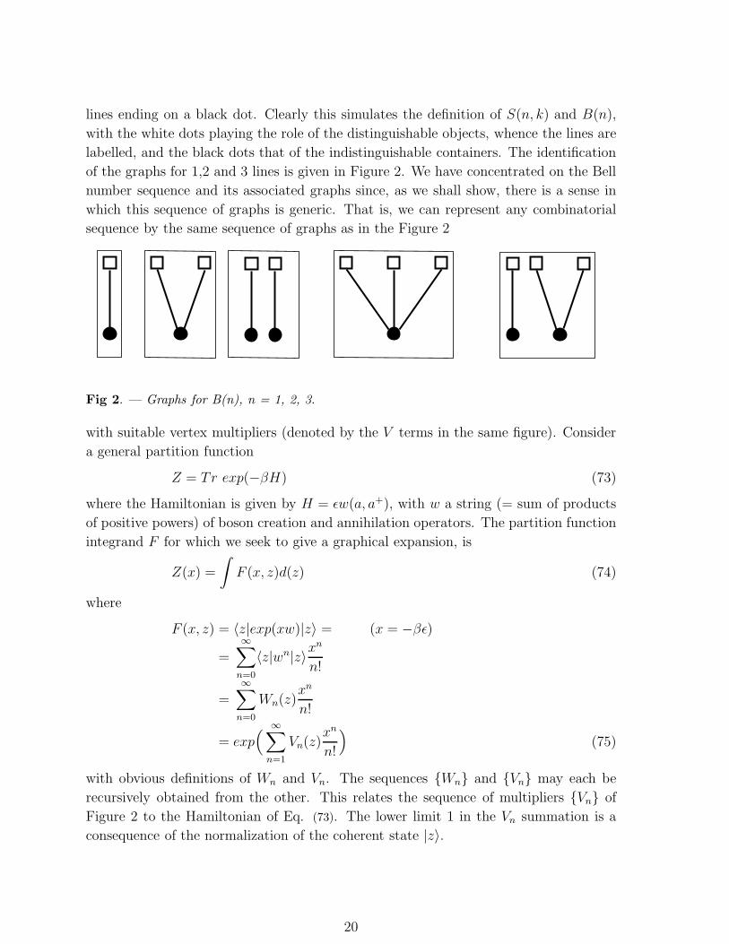
lines ending on a black dot. Clearly this simulates the definition of S(n, k) and B(n),

with the white dots playing the role of the distinguishable objects, whence the lines are

labelled, and the black dots that of the indistinguishable containers. The identification

of the graphs for 1,2 and 3 lines is given in Figure 2. We have concentrated on the Bell

number sequence and its associated graphs since, as we shall show, there is a sense in

which this sequence of graphs is generic. That is, we can represent any combinatorial

sequence by the same sequence of graphs as in the Figure 2

Fig 2. — Graphs for B(n), n = 1, 2, 3.

with suitable vertex multipliers (denoted by the V terms in the same figure). Consider

a general partition function

Z = Tr exp(−βH) (73)

where the Hamiltonian is given by H = ǫw(a, a+), with w a string (= sum of products

of positive powers) of boson creation and annihilation operators. The partition function

integrand F for which we seek to give a graphical expansion, is

Z(x) =

∫

F (x, z)d(z) (74)

where

F (x, z) = 〈z|exp(xw)|z〉 = (x = −βǫ)

=∞∑

n=0

〈z|wn|z〉xn

n!

=

∞∑

n=0

Wn(z)xn

n!

= exp(

∞∑

n=1

Vn(z)xn

n!

)

(75)

with obvious definitions of Wn and Vn. The sequences {Wn} and {Vn} may each be

recursively obtained from the other. This relates the sequence of multipliers {Vn} of

Figure 2 to the Hamiltonian of Eq. (73). The lower limit 1 in the Vn summation is a

consequence of the normalization of the coherent state |z〉.

20

7.4. The Hopf Algebra LBell

We briefly describe the Hopf algebra LBell which the diagrams of Figure 2 define.

1. Each distinct diagram is an individual basis element of LBell ; thus the dimension is

infinite. (Visualise each diagram in a “box”.) The sum of two diagrams is simply the

two boxes containing the diagrams. Scalar multiples are formal; for example, they may

be provided by the V coefficients. Precisely, as a vector space, LBell is the space freely

generated by the diagrams of Figure 2 (see APPENDIX : Function Spaces).

2. The identity element e is the empty diagram (an empty box).

3. Multiplication is the juxtaposition of two diagrams within the same “box”. LBell is

generated by the connected diagrams; this is a consequence of the Connected Graph

Theorem [34]. Since we have not here specified an order for the juxtaposition, multipli

cation is commutative.

4. The comultiplication ∆ : LBell 7→ LBell ⊗ LBell is defined by

∆(e) = e⊗ e (unit e, the empty box)

∆(x) = x⊗ e+ e⊗ x (generator x)

∆(AB) = ∆(A)∆(B) otherwise

so that ∆ is an algebra homomorphism. (76)

8. The case of two modes

Let us consider an hamiltonian on two modes H(a, a+, b, b+), with

[a, a+] = 1

[b, b+] = 1

[aǫ1, bǫ2 ] = 0, ǫi being + or empty (4 relations) (77)

Suppose that one can express H as

H(a, a+, b, b+) = H1(a, a+) +H2(b, b

+). (78)

and that, exp(λH1) and exp(λH2) (λ = −β) are solved i.e. that we have expressions

F (λ) = exp(λH1) =

∞∑

n=0

λn

n!H

(n)1 (a, a+) ; G(λ) = exp(λH2) =

∞∑

n=0

λn

n!H

(n)2 (b, b+) (79)

It is not difficult to check that

exp(λH) = exp(

λ(H1 +H2))

= F (λd

dx)G(x)

∣

∣

∣

x=0(80)

This leads us to define, in general, the “Hadamard exponential product”. Let

F (z) =∑

n≥0

anzn

n!, G(z) =

∑

n≥0

bnzn

n!(81)

and define their product (the “Hadamard exponential product”) by

21

H(F,G) :=∑

n≥0

anbnzn

n!= H(F,G) = F

(

zd

dx

)

G(x)

∣

∣

∣

∣

x=0

. (82)

When F (0) andG(0) are not zero one can normalize the functions in this bilinear product

so that F (0) = G(0) = 1. We would like to obtain compact and generic formulas. If we

write the functions as

F (z) = exp

(

∞∑

n=1

Lnzn

n!

)

and G(z) = exp

(

∞∑

n=1

Vnzn

n!

)

. (83)

that is, as free exponentials, then by using Bell polynomials in the sets of variables L,V

(see [21, 26] for details), we obtain

H(F,G) =∑

n≥0

zn

n!

∑

P1,P2∈UPn

LType(P1)V

Type(P2) (84)

where UPn is the set of unordered partitions of [1 · · ·n]. An unordered partition P of a

set X is a collection of (nonempty) subsets of X , mutually disjoint and covering X (i.e.

the union of all the subsets is X , see [28] for details).

The type of P ∈ UPn (denoted above by Type(P )) is the multi-index (αi)i∈N+ such that

αk is the number of k-blocks, that is the number of members of P with cardinality k.

At this point the formula entangles and the diagrams of the theory arise.

Note particularly that

• the monomial LType(P1)VType(P2) needs much less information than that which is

contained in the individual partitions P1, P2 (for example, one can relabel the

elements without changing the monomial),

• two partitions have an incidence matrix from which it is still possible to recover the

types of the partitions.

The construction now proceeds as follows.

(i) Take two unordered partitions of [1 · · ·n], say P1, P2.

(ii) Write down their incidence matrix (card(Y ∩ Z))(Y,Z)∈P1×P2.

(iii) Construct the diagram representing the multiplicities of the incidence matrix : for

each block of P1 draw a black spot (resp. for each block of P2 draw a white spot).

(iv) Draw lines between the black spot Y ∈ P1 and the white spot Z ∈ P2; there are

card(Y ∩ Z) such.(v) Remove the information of the blocks Y, Z, · · ·.In so doing, one obtains a bipartite graph with p (= card(P1)) black spots, q (= card(P2))

white spots, no isolated vertex and integer multiplicities. We denote the set of such

diagrams by diag.

22

♠ ♠ ♠ ♠

⑥ ⑥ ⑥

{1} {2, 3, 4} {5, 6, 7, 8, 9} {10, 11}

{2, 3, 5} {1, 4, 6, 7, 8} {9, 10, 11}

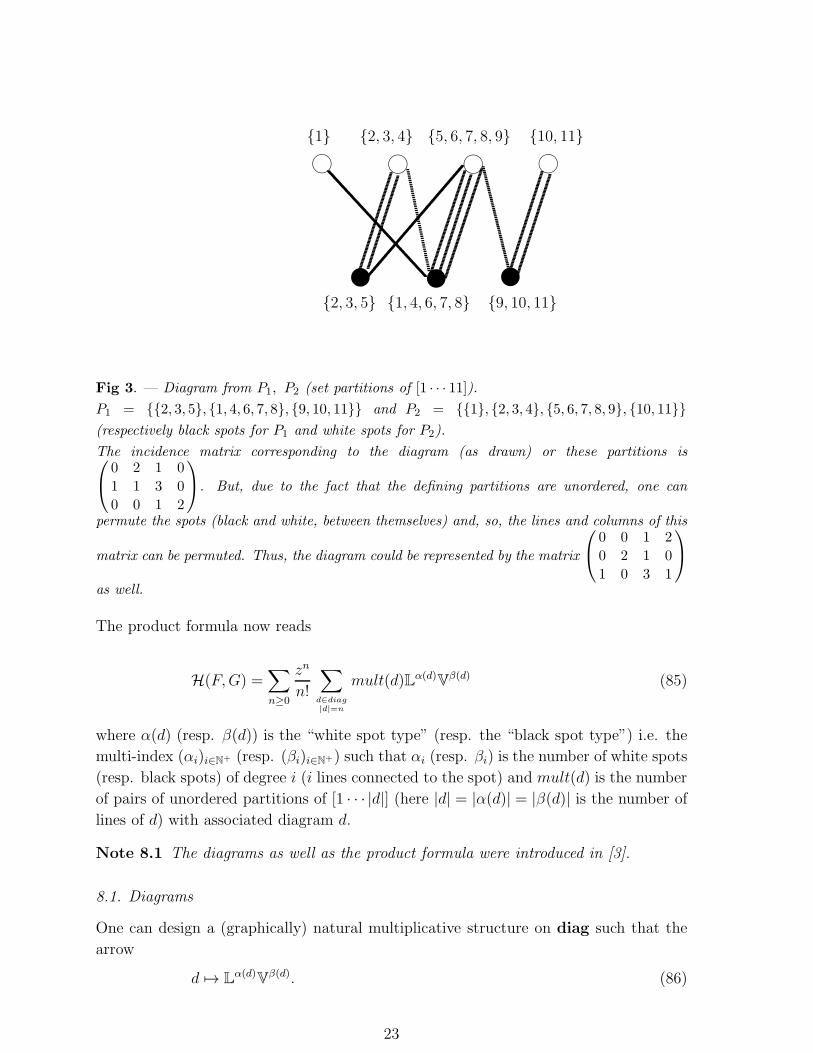
Fig 3. — Diagram from P1, P2 (set partitions of [1 · · · 11]).P1 = {{2, 3, 5}, {1, 4, 6, 7, 8}, {9, 10, 11}} and P2 = {{1}, {2, 3, 4}, {5, 6, 7, 8, 9}, {10, 11}}(respectively black spots for P1 and white spots for P2).

The incidence matrix corresponding to the diagram (as drawn) or these partitions is

0 2 1 0

1 1 3 0

0 0 1 2

. But, due to the fact that the defining partitions are unordered, one can

permute the spots (black and white, between themselves) and, so, the lines and columns of this

matrix can be permuted. Thus, the diagram could be represented by the matrix

0 0 1 2

0 2 1 0

1 0 3 1

as well.

The product formula now reads

H(F,G) =∑

n≥0

zn

n!

∑

d∈diag

|d|=n

mult(d)Lα(d)V

β(d) (85)

where α(d) (resp. β(d)) is the “white spot type” (resp. the “black spot type”) i.e. the

multi-index (αi)i∈N+ (resp. (βi)i∈N+) such that αi (resp. βi) is the number of white spots

(resp. black spots) of degree i (i lines connected to the spot) and mult(d) is the number

of pairs of unordered partitions of [1 · · · |d|] (here |d| = |α(d)| = |β(d)| is the number of

lines of d) with associated diagram d.

Note 8.1 The diagrams as well as the product formula were introduced in [3].

8.1. Diagrams

One can design a (graphically) natural multiplicative structure on diag such that the

arrow

d 7→ Lα(d)

Vβ(d). (86)

23

be a morphism. This is provided by the concatenation of the diagrams (the result, i.e.

the diagram obtained in placing d2 at the right of d1, will be denoted by [d1|d2]D). One

must check that this product is compatible with the equivalence of the permutation of

white and black spots among themselves, which is rather straightforward (see [21, 28]).

We have

Proposition 8.2 [28] Let diag be the set of diagrams (including the empty one).

i) The law (d1, d2) 7→ [d1|d2]D endows diag with the structure of a commutative monoid

with the empty diagram as neutral element(this diagram will, therefore, be denoted by

1diag).

ii) The arrow d 7→ Lα(d)Vβ(d) is a morphism of monoids, the codomain of this arrow

being the monoid of (commutative) monomials in the alphabet L ∪ V i.e.

MON(L ∪ V) = {LαV

β}α,β∈(N+)(N) =⋃

n,m≥1

{Lα11 L

α22 · · ·Lαn

n V β1

1 V β2

2 · · ·V βm

m }αi,βj∈N. (87)

iii) The monoid (diag, [−|−]D, 1diag) is a free commutative monoid. The set on which

it is built is the set of the connected (non-empty) diagrams.

Remark 8.3 The reader who is not familiar with the algebraic structure of MON(X)

can find rigorous definitions in paragraph (12.2).

We denote φmon,diag the arrow diag 7→MON(L ∪ V).

8.2. Labelled diagrams

We have seen the diagrams (of diag) are in one-to-one correspondence with classes of

matrices as in Fig. 3. In order to fix one representative of this class, we have to number

the black (resp. white) spots from 1 to, say p (resp. q). Doing so, one obtains a packed

matrix [25] that is, a matrix of integers with no row nor column consisting entirely of

zeroes. In this way, we define the labelled diagrams.

Definition 8.4 A labelled diagram of size p × q is a bi-coloured (vertices are p black

and q white spots) graph

• with no isolated vertex

• every black spot is joined to a white spot by an arbitrary quantity (but a positive

integer) of lines

• the black (resp. white) spots are numbered from 1 to p (resp. from 1 to q).

As in paragraph (8.1), one can concatenate the labelled diagrams, the result, i.e. the

diagram obtained in placing D2 at the right of D1, will be denoted by [D1|D2]L. This

time we need not check compatibility with classes. We have a structure of free monoid

(but not commutative this time)

24

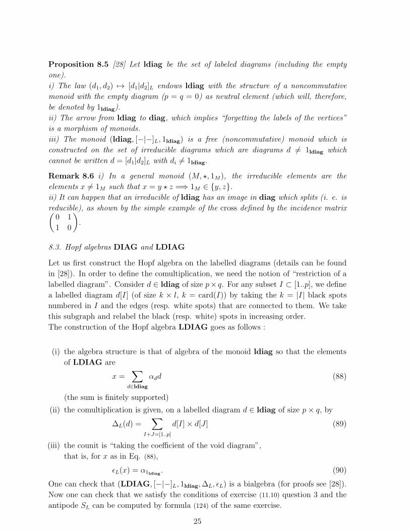
Proposition 8.5 [28] Let ldiag be the set of labeled diagrams (including the empty

one).

i) The law (d1, d2) 7→ [d1|d2]L endows ldiag with the structure of a noncommutative

monoid with the empty diagram (p = q = 0) as neutral element (which will, therefore,

be denoted by 1ldiag).

ii) The arrow from ldiag to diag, which implies “forgetting the labels of the vertices”

is a morphism of monoids.

iii) The monoid (ldiag, [−|−]L, 1ldiag) is a free (noncommutative) monoid which is

constructed on the set of irreducible diagrams which are diagrams d 6= 1ldiag which

cannot be written d = [d1|d2]L with di 6= 1ldiag.

Remark 8.6 i) In a general monoid (M, ⋆, 1M), the irreducible elements are the

elements x 6= 1M such that x = y ⋆ z =⇒ 1M ∈ {y, z}.ii) It can happen that an irreducible of ldiag has an image in diag which splits (i. e. is

reducible), as shown by the simple example of the cross defined by the incidence matrix(

0 1

1 0

)

.

8.3. Hopf algebras DIAG and LDIAG

Let us first construct the Hopf algebra on the labelled diagrams (details can be found

in [28]). In order to define the comultiplication, we need the notion of “restriction of a

labelled diagram”. Consider d ∈ ldiag of size p× q. For any subset I ⊂ [1..p], we define

a labelled diagram d[I] (of size k × l, k = card(I)) by taking the k = |I| black spots

numbered in I and the edges (resp. white spots) that are connected to them. We take

this subgraph and relabel the black (resp. white) spots in increasing order.

The construction of the Hopf algebra LDIAG goes as follows :

(i) the algebra structure is that of algebra of the monoid ldiag so that the elements

of LDIAG are

x =∑

d∈ldiag

αdd (88)

(the sum is finitely supported)

(ii) the comultiplication is given, on a labelled diagram d ∈ ldiag of size p× q, by∆L(d) =

∑

I+J=[1..p]

d[I]× d[J ] (89)

(iii) the counit is “taking the coefficient of the void diagram”,

that is, for x as in Eq. (88),

ǫL(x) = α1ldiag. (90)

One can check that (LDIAG, [−|−]L, 1ldiag,∆L, ǫL) is a bialgebra (for proofs see [28]).

Now one can check that we satisfy the conditions of exercise (11.10) question 3 and the

antipode SL can be computed by formula (124) of the same exercise.

25

We have so far constructed the Hopf algebra (LDIAG, [−|−]L, 1ldiag,∆, ǫ, SL).

The constructions above are compatible with the arrow

φDIAG,LDIAG : LDIAG 7→ DIAG

deduced from the class-map φdiag,ldiag : ldiag 7→ diag (a diagram is a class of labelled

diagrams under permutations of black and white spots among themselves). So that,

one can deduce “by taking quotients” a structure of Hopf algebra on the algebra of

diag. Denoting this algebra by DIAG, one has a natural Hopf algebra structure

(DIAG, [−|−]D, 1diag,∆D, ǫD, SD) and one can prove that this is the unique Hopf

algebra structure such that φDIAG,LDIAG is a morphism for the algebra and coalgebra

structures.

9. Link between LDIAG and other Hopf algebras

9.1. The deformed case

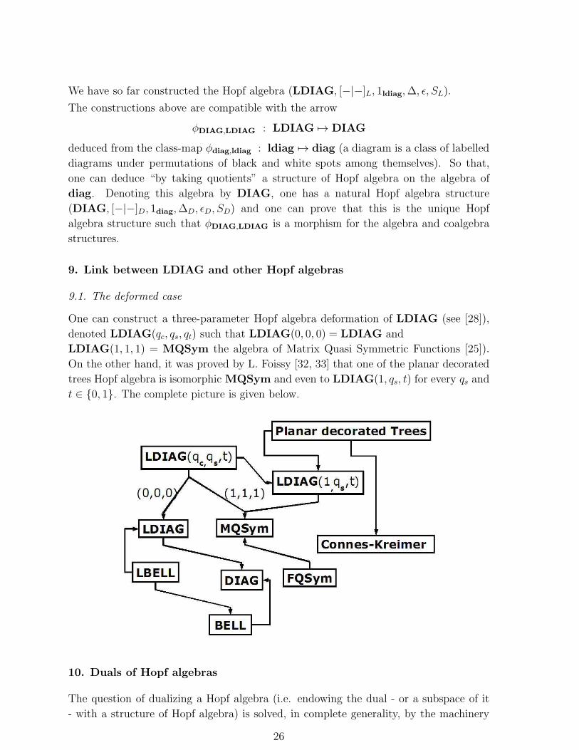
One can construct a three-parameter Hopf algebra deformation of LDIAG (see [28]),

denoted LDIAG(qc, qs, qt) such that LDIAG(0, 0, 0) = LDIAG and

LDIAG(1, 1, 1) = MQSym the algebra of Matrix Quasi Symmetric Functions [25]).

On the other hand, it was proved by L. Foissy [32, 33] that one of the planar decorated

trees Hopf algebra is isomorphic MQSym and even to LDIAG(1, qs, t) for every qs and

t ∈ {0, 1}. The complete picture is given below.

10. Duals of Hopf algebras

The question of dualizing a Hopf algebra (i.e. endowing the dual - or a subspace of it

- with a structure of Hopf algebra) is solved, in complete generality, by the machinery

26

of Sweedler’s duals. The procedure consists in taking the “representative” linear forms

(instead of all the linear forms) and dualize w.r.t. the following table

comultiplication → multiplication

counit → unit

multiplication → comultiplication

unit → counit

antipode → trsnspose of the antipode.

In the case when the Hopf algebra is free as an algebra (which is often the case with

noncommutative Hopf algebras of combinatorial physics), one can use rational expres-

sions of Automata Theory to get a genuine calculus within this dual (see [29]).

27

11. EXERCISES

Exercise 11.1 Representative functions on R (Complex valued). A function

Rf−→ C is said to be representative if there exist (f

(1)i )ni=1 and (f

(2)i )ni=1 such that, for

all x, y ∈ R one has

f(x+ y) =n∑

i=1

f(1)i (x)f

(2)i (y). (91)

1) Show that cos, cos2, sin, exp and a→ an are representative. Provide minimal sums

of type Eq.(91).

2) Show that the following are equivalent

i) f is representative.

ii) There exists a group representation (R,+)ρ−→ Cn×n, a row vector λ ∈ C1×n, a

column vector γ ∈ Cn×1 such that f(x) = λρ(x)γ.

iii) (ft)t∈R is of finite rank in CR (here ft, the shift of f by t, is the function

x −→ f(x+ t)).

3) Show that the minimal n such that formula Eq.(91) holds is also the rank (over C)

of (ft)t∈R.

4) a) If f is continuous then ρ can be chosen so and ρ(x) = exT for a certain matrix

T ∈ Cn×n.

b) In this case show that representative functions are linear combinations of products of

polynomials and exponentials.

5) f ∈ CR is representative iff Re(f) = (f + f)/2 and Im(f) = (f − f)/2i are

representative in RR.

6) Show that the set of representative functions of CR is a C-vector space. This space

will be denoted RepC(R).

7) Show that the functions ϕn,λ = xneλx are a basis of RepC(R) ∩ Co(R;C) (i.e.

continuous complex valued representative functions on R).

8) Deduce from (7) that the following statement is false:

“If a entire function f : R 7→ C is such that (ft)t∈Z is of finite rank, then it is

representative”. Hint : Consider exp(exp(2iπx)).

Exercise 11.2 Representative functions in general (see also [1, 20]) Let M be

a monoid (semigroup with unit) and k a field (one can first think of k = R,C). For a

function Mf−→ k one defines the shifts:

fz : x −→ f(zx),

yf : x −→ f(xy),

yfz : x −→ f(zxy). (92)

1)a) Check the following formulas

(fy1)y2 = fy1y2,

y2(y1f) =y2y1 f

(xf)y =x (fy) =x fy. (93)

28

As for groups, if M is a monoid, a M-module structure on a vector space V is defined

by a morphism or an anti-morphism M 7→ Endk(V ).

b) From Eqs.(93) define two canonical M-module structures of kM .

2)a) Show that the following are equivalent

i) (fz)z∈M is of finite rank in kM .

ii) (yf)y∈M is of finite rank in kM .

iii) (yfz)y,z∈M is of finite rank in kM .

iv) There exist two families (f(1)i )ni=1 and (f

(2)i )ni=1 such that

f(xy) =

n∑

i=1

f(1)i (x)f

(2)i (y). (94)

v) There exists a representation of M ρ :M −→ kn×n, a row vector λ ∈ k1×n, a column

vector γ ∈ kn×1 such that f(x) = λρ(x)γ for all x ∈M .

b) Using (v) above, show that the (pointwise) product of two representative functions is

representative.

One denotes Repk(M) the space of (k-valued) representative functions on M .

3) a) Recall briefly why the mapping

kM ⊗ kM 7→ kM×M (95)

defined byn∑

i=1

f(1)i ⊗ f

(2)i →

(

(x, y)→n∑

i=1

f(1)i (x)f

(2)i (y)

)

is injective.

b) Show that, if n is minimal in (94), the families of functions f(1)i and f

(2)i are

representative and that the mapping Repk(M) 7→ Repk(M)⊗ Repk(M) defined by

f →n∑

i=1

f(1)i ⊗ f

(2)i (96)

defines a structure of coassociative coalgebra on Repk(M) Has it a co-unit ?

We denote by ∆ the compultiplication contructed above.

4) Show that (Repk(M), ., 1,∆, ǫ1M ) (with 1 the constant-valued function equal to 1 on

M and ǫ the Dirac measure f → f(1M)) is a bialgebra.

Exercise 11.3 (Example of a monoid coming from dissipation theory [47]).

Let (Mn,×) be the monoid of n × n complex square matrices endowed with the usual

product

(Mn, .) = (Cn×n,×)We define a state (Von Neumann) as a positive semi-definite hermitian matrix of trace

one (= 1) i.e. a matrix ρ such that

(i) ρ = ρ∗

(ii) (∀x ∈ Cn×1)(x∗ρx ≥ 0)

29

(iii) Tr(ρ) = 1.

The set of such states will be denoted by Sn.1) (Structure) a) Show that Sn is convex.b) Show that Sn is compact.Hint : Consider the set of possible spectra i.e. the simplex

S = {(λ1, λ2, · · · , λn) ∈ (R+)n|n∑

i=1

λi = 1}

and show that Sn is the range of the continuous mapping φ : U(n)× S 7→ Mn given by the formula

φ(u, s) = udu∗ ; with d =

λ1 0 · · · 0

0 λ2 · · · 0. . .

0 · · · 0 λn

(97)

and where s = (λ1, λ2, · · · , λn).

c) Show that the extremal elements [9] of the compact Sn is the set of orthogonal

projections of rank one and that this set is connected by arcs.

2) (KS condition) We say that a finite family (ki)i∈I (I is finite) of elements in Mn

fulfils the KS condition iff∑

i∈I k∗i ki = In (In is the unity matrix, the unit of the monoid

Mn).

On the other hand, given two finite families A = (ki)i∈I and B = (lj)j∈J , we define

A ∗B as the family

A ∗B = (kilj)(i,j)∈I×J (98)

a) Show that, if A and B fulfil the KS condition then so too does A ∗B.

To every (finite) family A = (ki)i∈I which fulfils the KS condition, we attach a

transformation φA :Mn 7→ Mn, given by the formula

φA(M) =∑

i∈I

kiMk∗i (99)

b) Show that φA is linear and preserves Sn (i.e. φA(Sn) ⊂ Sn).c) Show that if A and B fulfil the KS condition, one has

φA ◦ φB = φA∗B (100)

Conclude that the φA form a semigroup of transformations (with unit).

d) (Example) Let (Ei,j)i,j∈{1,2} be the set of the four matrix units inM2. Show that the

following families fulfil KS condition

A = (E11,1

√

(2)E12,

1√

(2)E22)

B = (1

√

(2)E11,

1√

(2)E21, E22) (101)

Compute A ∗B.

3) (Description of the semigroup at the level of multisets). In order to pull-back the

formula (100) at the level of multisets, we remark that the order or the labelling of the

30

elements ki is irrelevant; all that counts is their multiplicities.

a) (Example showing that the “set” structure is too weak). Let (Ei,j)i,j∈{1,2} be the set

of the four matrix units inM2 and set

A = (1

√

(2)E11,

1√

(2)E12,

1√

(2)E21,

1√

(2)E22) (102)

compute A ∗A and check that it has (non-zero) repeated elements and thus corresponds

to a multiset (see appendix).

b) Show that the multisets ofMn are exactly the elements∑

M∈MnλM [M ] (here we note

[M ] the image of M ∈Mn in the algebra R[Mn] in order to forbid matrix addition) of

the algebra R[Mn] such that

(∀M ∈ Mn)(λM ∈ N) (103)

the set of elements fulfilling (103) will be denoted N[Mn].

b) To every finite family of matrices (inMn) A = (Mi)i∈I one may associate its sum (in

R[Mn]) S(A) =∑

i∈I Mi, check that it is an element of N[Mn] and that every element

of N[Mn] is obtained so.

c) Show that S(A ∗ B) = S(A).S(B) ∈ N[Mn] ⊂ R[Mn] and deduce that (N[Mn], .) is

a monoid.

d) To every multiset of matrices (inMn) A =∑

M∈Mnα(M)[M ], one associates

T (A) =∑

M∈Mn

α(M)[M∗M ]

show that, if A = (Mi)i∈I is a finite set of matrices, one has∑

i∈I

M∗i Mi = T (S(A)) (104)

e) Show that, if T (A) = In, T (A.B) = T (B).

We denote N[Mn]KS the set of A ∈ N[Mn] such that T (A) = In.

f) Check that the mapping φA defined previously depends only on S(A) and denote, for

A ∈ N[Mn]KS the mapping ΦA deduced from this property.

g) Prove that the mapping (N[Mn]KS, .) 7→ (EndC(C

n×n), ◦) is a morphism of

semigroups (preserving the units).

4) (Invertible elements) To every A =∑

M∈Mnα(M)[M ] ∈ N[Mn]

KS one associates

ǫ(A) =∑

M∈Mnα(M) ∈ N.

a) Prove that

ǫ(A.B) = ǫ(A)ǫ(B) (105)

b) Prove that

ǫ(A) = 1 =⇒ |supp(α)| = 1 (106)

and, thus, in this condition, A = [M ] (a single matrix).

c) Deduce from (a) and (b) that the set of invertible elements of N[Mn]KS is exactly the

unitary group U(n).

31

Exercise 11.4 Let (M, ∗, 1M) be a monoid, ≡ an equivalence relation on M and

Cl : M 7→ M/ ≡ the class function (which, to every element of M associates its class

Cl(x)).

a) Suppose that there is an (internal) law ⊥ on M/ ≡ such that Cl is a morphism i.e.

one has

(∀x, y ∈M)(Cl(x ∗ y) = Cl(x) ⊥ Cl(y)) (107)

then prove that ≡ is compatible with the right and left “translations” of the monoid this

means that

(∀ x, y, t, s ∈ S)(x ≡ y =⇒ [s ∗ x ∗ t ≡ s ∗ y ∗ t]) (108)

b) Conversely, we suppose that ≡ is an equivalence on M satisfying condition (108),

show that the result Cl(x′ ∗ y′) does not depend on the choice of x′ ∈ Cl(x); y′ ∈ Cl(x)and therefore construct a law ⊥ on M/ ≡ such that the class function is a morphism

(i.e. (107)).

c) Show moreover that, in the preceding conditions,(

M/ ≡,⊥, Cl(1M))

is a monoid.

Exercise 11.5 Let A be an AAU and ∆ : A 7→ A ⊗ A a comultiplication. We build

(tensor) products of two representations by the formula (24), more precisely by

can ◦ (ρ1 ⊗ ρ2) ◦∆ (109)

where can : End(V1)⊗ End(V2) 7→ End(V1 ⊗ V2) is the canonical mapping.

a) Prove that, if ∆ is a morphism of algebras, then the linear mapping

ρ1×

ρ2 : A 7→ End(V1 ⊗ V2) (110)

defined by the composition (109) is a morphism of AAU (and hence a representation).

b) Prove that, if ρ1×

ρ2 is a representation for any pair ρ1, ρ2 of representations of A,then ∆ is a morphism of AAU (use ρ1 = ρ2, the - regular - representation of A on itself

by multiplications on the left).

Exercise 11.6 We consider the canonical isomorphisms

can1|23 : V1 ⊗ (V2 ⊗ V3) 7→ V1 ⊗ V2 ⊗ V3can12|3 : (V1 ⊗ V2)⊗ V3 7→ V1 ⊗ V2 ⊗ V3 (111)

Show that, in order to have (37) for every triple ρi, i = 1, 2, 3 of representations it is

necessary and sufficient that

can12|3 ◦ (∆⊗ IdA) ◦∆ = can1|23 ◦ (IdA ⊗∆) ◦∆ (112)

(for the necessary condition, consider again the left regular representations).

Exercise 11.7 Let (A,∆) be a coalgebra (∆ is an arbitrary - but fixed - linear mapping)

and (A∗, ∗∆) be its dual algebra. Explicitely, for f, g ∈ A∗ and x ∈ A (for convenience,

the law is written in infix denotation)

〈f ∗∆ g|x〉 = 〈f ⊗ g|∆(x)〉 (113)

32

Prove the following equivalences

∆ is co-associative ⇐⇒ ∗∆ is associative (114)

(∀ǫ ∈ A∗)(

ǫ is a unity for (A∗, ∗∆)⇐⇒ ǫ is a co-unity for (A,∆))

(115)

Exercise 11.8 The mappings canl, canr are as in (41). Prove that, in order that for

any representation ρ of A, one has

canl ◦ (ǫ⊗ ρ) ◦∆ = canr ◦ (ρ⊗ ǫ) ◦∆ (116)

it is necessary and sufficient that ǫ be a counit.

Exercise 11.9 Let (C,∆) be a coalgebra and (A, µ) ba an algebra on the same

(commutative) field of scalars k. We define a multiplication (called convolution) on

Homk(C,A) byf ∗ g = µ ◦ (f ⊗ g) ◦∆ (117)

so that, if ∆(x) =∑

(1)(2) x(1)x(2),

f ∗ g(x) =∑

(1)(2)

f(x(1))g(x(2)).

1) If A is associative and C coassociative, show that the algebra (Homk(C,A), ∗) is

associative.

2) We suppose moreover that C admits a counit ǫ : C 7→ k and A a unit 1A (identified

with the linear mapping k 7→ A given by λ→ λ1A).

Show that 1A ◦ ǫ (traditionnally denoted 1Aǫ) is the unit of the algebra (Homk(C,A), ∗).3) Let (B, ∗, 1,∆, ǫ) be a bialgebra. The convolution under consideration will be that

constructed between the coalgebra (B,∆, ǫ) and the algebra (B, ∗, 1).a) Let S ∈ End(B). Show that the following are equivalent

i) S is an antipode for Bii) S is the inverse of IdB in (Endk(B), ∗).b) Deduce from (b) that the antipode, if it exists, is unique.

c) Prove that the bialgebra (k〈A〉, ∗,∆h, ǫaug) defined around equation (50) admits no

antipode (if the alphabet A is not empty).

4) Let (C,∆, ǫ) be a coalgebra coassociative with counit. We define ∆2 by T2,3 ◦∆ ⊗∆

where T2,3 : C⊗4 7→ C⊗4 is the flip between the 2nd and the 3rd component

T2,3(x1 ⊗ x2 ⊗ x3 ⊗ x4) = x1 ⊗ x3 ⊗ x2 ⊗ x4 (118)

a) Show that (C ⊗ C,∆2, ǫ⊗ ǫ) (with ǫ⊗ ǫ(x ⊗ y) = ǫ(x)ǫ(y)) is coassociative coalgebra

with counit.

Let (H, µ, 1,∆, ǫ, S) be a Hopf algebra. The convolution ∗ here will be that constructed

between the coalgebra (H⊗H,∆2, ǫ⊗ ǫ) and the algebra (H, µ, 1). We consider the two

elements νi ∈ (Homk(H ⊗ H,H), ∗) defined by ν1 = S ◦ µ and ν2(x ⊗ y) = S(y)S(x).

b) Show that the elements νi are the convolutional inverses of µ. Deduce from this that

S : H 7→ H is an antimorphism of algebras.

33

Exercise 11.10 1) Let (B, ∗, 1,∆, ǫ) be a bialgebra, we denote by B+ the kernel of ǫ.

a) Prove that B = B+ ⊕ k.1B.We denote I+ the projection B 7→ B+ with respect to the preceding decomposition.

b) Prove that, for every x ∈ B+, one can write

∆(x) = x⊗ 1 + 1⊗ x+∑

(1)(2)

x(1) ⊗ x(2) with x(i) ∈ B+ (119)

2) Define for x ∈ B+,

∆+(x) = ∆(x)− (x⊗ 1 + 1⊗ x) =∑

(1)(2)

x(1) ⊗ x(2) (120)

a) Check that (B+,∆+) is a coassociative coalgebra.

Define

(B∗)+ = {f ∈ B∗|f(1) = 0} (121)

b) Prove that (B∗)+ is a subalgebra of (B, ∗∆) and that its law is dual of ∆+.

c) Prove that the algebra (B∗, ∗∆) is obtained from(

(B∗)+, ∗∆+

)

by adjunction of the

unity ǫ.

3) The bialgebra is called locally finite if

(∀x ∈ B)(∃k ∈ N∗)(∆+(k)(x) = 0). (122)

The projection I+ being as above, show that, in case B is locally finite,

(∀x ∈ B)(∃N ∈ N∗)(∀k ≥ N)((I+)k(x) = 0) (123)

and that

S =∑

n∈N

(−I+)n (124)

is an antipode for B.

Exercise 11.11 1) Let G be a group and H = (C[G], ., 1G,∆, ǫ, S) be the Hopf algebra

of G.

a) Show that {(g− 1)}g∈G−{1} is a basis of H+ (defined as above) and that ∆+(g− 1) =

(g − 1)⊗ (g − 1).

b) Show that, if G 6= {1}, H+ is not locally finite, but H admits an antipode.

2) Prove that, if the coproduct of H is graded (i.e. there exists a decomposition

H = ⊕n∈NHn with ∆(Hn) ⊂∑

a+b=nHa⊗Hb) and H0 = k.1H , then the comultiplication

is locally finite.

3) Define the degree of a labelled diagram as its number of edges and LDIAGn as

the vector space generated by the diagrams of degree n and check that we satisfy the

conditions of exercise (11.10) question 5.

Exercise 11.12 1) Show that, in order that a family (λki,j)i,j,k∈I be the family of

structure constants of some algebra it is necessary and sufficient that

(∀(i, j) ∈ I2)(

(λki,j)k∈I is finitely supported)

(125)

34

2) Similarly show that in order that a family (λj,ki )i,j,k∈I be the family of structure

constants of some coalgebra it is necessary and sufficient that

(∀i ∈ I)(

(λj,ki )(j,k)∈I2 is finitely supported)

(126)

3) Give examples of mappings λ : I3 7→ k such that the corresponding families satisfy

i) (125) and (126)

ii) (125) and not (126)

iii) (126) and not (125)

iv) none of (125) and (126)

4) Give further examples such as those in 3) i-iii but now defining associative (resp.

coassociative) multiplications (resp. comultiplications).

12. APPENDIX

12.1. Function spaces

Throughout the text, we use the basic constructions of set theory and algebra (see [6, 7]).

The set of mappings between two sets X and Y is denoted by Y X . Thus if k is a field

kX = {f : X −→ k} (127)

the vector space of all functions defined onX with values in k. For each function f ∈ kX ,we call the “support of f” the set of points x ∈ X such that f(x) is not zero+.

supp(f) = {x ∈ X : f(x) 6= 0} (128)

the set of functions with finite support is a vector subspace of kX which is denoted by

k(X).

An interesting extension of this notion to other sets of coefficients is the combinatorial

notion of (finite) multisets.

Recall that a multiset is a (set with repetitions) [40]. For example, the first multisets

with elements from {a, b} are{}, {a}, {b}, {a, a}, {a, b}, {b, b}, {a, a, a}, {a, a, b}, {a, b, b}, {b, b, b},{a, a, a, a}, {a, a, a, b}, {a, a, b, b}, {a, b, b, b}, {b, b, b, b}, · · · . (129)

A multiset with elements in X is then described equivalently by a multiplicity function

α : X 7→ N with finite support. The support of such a mapping is defined as in

(128) and the set of finite multiplicity functions will be denoted by N(X) (see below the

free commutative monoid (12.4)). For example, the multiplicity functions {a, b} 7→ N

corresponding to the multisets given in (130) are, in the same order (we characterize α

by the pair (α(a), α(b)))

(0, 0), (1, 0), (0, 1), (2, 0), (1, 1), (0, 2), (3, 0), (2, 1), (1, 2), (0, 3),

(4, 0), (3, 1), (2, 2), (1, 3), (0, 4), · · · (130)

+ In integration theory, the support of a function is the closure of what we define as the (algebraic)

support.

35

12.2. Basic structures

Definition 12.1 (Semigroup) A semigroup (S, ∗) is a set S endowed with a closed

binary operation ∗ satisfying an associative law, this means that, for all x, y, z ∈ S

one has x ∗ (y ∗ z) = (x ∗ y) ∗ z.

http://en.wikipedia.org/wiki/Semigroup

Definition 12.2 (Monoid) A monoid (M, ∗) is a semigroup which possesses a neutral

element, i.e. an element e ∈M such that, for all x ∈M :

e ∗ x = x ∗ e = x. (131)

Such an element, if it exists is unique. The neutral element is often denoted 1M .

http://en.wikipedia.org/wiki/Monoid

Definition 12.3 (Free Monoid) The free monoid of alphabet X is the set of strings

x1x2 · · ·xn with letters xi ∈ X (comprising the empty string). This set is denoted X∗,

its law is the concatenation and its neutral element is the empty string.

It is easily seen that this monoid is free in the following sense. For any “set-theoretical”

mapping φ : X 7→M , where (M, ∗) is a monoid, φ can be extended to strings so that

Xφ //

can!!CC

CCCC

CCM

X∗

φ

OO(132)

Definition 12.4 (Free Commutative Monoid) The free commutative monoid of the

alphabet X is the set of monomials Xα (α ∈ N(X)). This set is denoted by MON(X)

and its law is the multiplication of monomials

XαXβ = Xα+β (133)

It is easily seen that this monoid is free in the following sense. For any “set-theoretical”

mapping φ : X 7→ M , where (M, ∗) is a commutative monoid, φ can be extended to

monomials so that

Xφ //

can %%JJJJJJJJJJ M

MON(X)

φ

OO

(134)

An interesting application of the free monoid is the explicit construction of a monoid

defined “by generators and relations”.

Let X be a set (of generators) and R = (ui, vi)i∈I a family of pairs of words, then one

can construct explicitely the smallest (i.e. the intersection of) congruence ≡R for which

(∀i ∈ I)(ui ≡ vi).

36

Let say that two words U, V ∈ X∗ are “related” by ≡R if there is a chain of replacements

of the type puis→ pvis or pvis→ puis p, s ∈ X∗ leading from U to V . Formally, there

exists a chain

U = U0, U1, · · ·Un = V (135)

such that for each j < n Uj = pjAqj ; Uj+1 = pjBqj with (A,B) = (ui, vi) or

(B,A) = (ui, vi) for some i (depending on j. One can show that the constructed ≡R is

a congruence (see exercise (108)) and we define

〈X ;R〉Mon (136)

as the quotient X∗/ ≡R. This monoid has the following property : if φX∗ 7→ M is a

morphism (of monoids) such that, for all i ∈ I one has φ(ui) = φ(vi), then φ factorises

uniquely through 〈X ;R〉Mon

Xφ //

can %%KKKKKKKKKK M

〈X ;R〉Mon

φ

OO

(137)

Definition 12.5 (Group) A group (G, ∗) is a monoid such that for each x ∈ G there

exists y such that

x ∗ y = y ∗ x = e. (138)

For fixed x such an element is unique and is usually denoted by x−1 and called the

inverse of x.

Definition 12.6 (Algebra of a monoid) Let k be a field (scalars, for example k = R or

C). The algebra k[M ] of a monoid M (with coefficients in k) is the set of mappings

k(M) endowed with the convolution product

f ∗ g(w) =∑

uv=w

f(u)g(v). (139)

The algebra (k[M ], ∗) is an AAU.

Each m ∈ M may be identified with its characteristic function (i.e. the Dirac function

δm with value 1 at m and 0 elsewhere). These functions form a basis of k[M ] and

then, every f ∈ k[M ] can be written as a finite sum f =∑

w f(w)w. Through this

identification the unity of M and k[M ] coincide.

The algebra of a monoid solves the following univeral problem.

Let M be a monoid and j : M 7→ k[M ] the embedding described above. For any AAU

A and any morphism of monoids φ : M 7→ A ((A, .) is a monoid), one has an unique

factorization

Mφ //

j��

A

k[M ]φ

<<zzzzzzzz

37

where φ is a morphism of AAU.

Likewise, the enveloping algebra Uk(G) of a Lie algebra G with the canonical mapping

can : Uk(G) 7→ G is the solution of a universal problem. The specifications are the

following

(i) Uk(G) is an AAU

(ii) can is a morphism of Lie algebras (for this, Uk(G) is endowed of the structure of

Lie algebra given by the bracket [X, Y ] = XY − Y X).

For any morphism of Lie algebras φ : G 7→ A (where A is endowed with the structure of

a Lie algebra given by the bracket [X, Y ] = XY − Y X), one has a unique factorization

Gφ //

can��

A

Uk(G)φ

<<yyyyyyyyy

(140)

where φ is a morphism of AAU.

38

References

[1] Abe E., Hopf Algebras, Cambridge University Press (2004).

[2] Bayen F., Flato M., Fronsdal C., Lichnerowicz A. and Sternheimer D., Deformation

and Quantization, Ann. of Phys. 111, (1978), pp. 61-151.

[3] Bender C.M., Brody D.C. and Meister, Quantum field theory of partitions, J. Math. Phys.

40, 3239 (1999)

[4] Berstel J., Reutenauer , Rational series and their languages EATCS Monographs on

Theoretical Computer Science, Springer (1988).

[5] Blasiak P., Horzela A., Penson K. A., Duchamp G. H. E. and Solomon A. I., Boson

normal ordering via substitutions and Sheffer-Type Polynomials, Phys. Lett. A 338 (2005)

108

[6] Bourbaki N., Theory of sets, Springer (2004)

[7] Bourbaki N., Algebra, chapter 1-III, Springer (2006)

[8] Bourbaki N., Algebra, chapter VI, Springer (2006)

[9] Bourbaki N., Topological Vector Spaces, Springer (2006)

[10] Bourbaki N., Integration I, Springer (2006)

[11] Broadhurst D. J., Kreimer D., Towards cohomology of renormalization: bigrading the

combinatorial Hopf algebra of rooted trees, Comm. Math. Phys. 215 (2000), no. 1, 217236,

hep-th/00 01202.

[12] Brouder C., Frabetti A., Renormalization of QED with planar binary trees,

arXiv:hep-th/0003202v1.

[13] Brouder C., Fauser B., Frabetti A., Oeckl R., Quantum field theory and Hopf algebra

cohomology, arXiv:hep-th/0311253v2.

[14] Brouder C., Trees, renormalization and differential equations, BIT 44 (2004), no. 3, 425438.

[15] Cartier P., A primer of Hopf algebras, Septembre (2006), IHES preprint IHES/M/06/40.

[16] Connes A., Kreimer D., Hopf algebras, Renormalization and Noncommutative geometry,

Comm. Math. Phys 199 (1998), 1, hep-th/98 08042.

[17] Connes A., Moscovici H., Hopf algebras, cyclic cohomology and the transverse index theorem,

Comm. Math. Phys. 198 (1998), 1, math.DG/98 06109.

[18] Cartier P., Foata D., Problemes combinatoires de commutation et rarrangements, 1969,

Springer-Verlag

Free electronic version available at

http://www-irma.u-strasbg.fr/∼foata/paper/pub11.html

[19] Chapoton F., Hivert F., Novelli J. -C. and Thibon J.-Y., An operational calculus for

the Mould operad, arXiv:0710.0349v3

[20] Chari V., Pressley A., A guide to quantum groups. Cambridge (1994).

[21] Duchamp G. H. E., Blasiak P., Horzela A., Penson K. A. and Solomon A. I.,

Feynman graphs and related Hopf algebras, Journal of Physics: Conference Series, SSPCM’05,

Myczkowce, Poland. arXiv : cs.SC/0510041

[22] G. Duchamp, Flouret M., Laugerotte E. and Luque J-G., Direct and dual laws for

automata with multiplicities, T.C.S. 267, 105-120 (2001).

arXiv : math.CO0607412

[23] Duchamp G., Krob D., Free partially commutative structures, Journal of Algebra 156, (1993)

318-361

[24] Duchamp G., Luque J-G., Congruences Compatible with the Shuffle Product, Proceedings,

(FPSAC 2000), D. Krob, A.A. Mikhalev Eds., Springer.

arXiv : math.CO0607419

[25] Duchamp G., Hivert F. and Thibon J. -Y., Non commutative functions VI: Free quasi-

symmetric functions and related algebras, International Journal of Algebra and Computation

12, No 5 (2002).

39

[26] Duchamp G., Solomon A. I., Penson K. A., Horzela A. and Blasiak P., One-parameter

groups and combinatorial physics, Proceedings of the Symposium Third International

Workshop on Contemporary Problems in Mathematical Physics (COPROMAPH3) (Porto-

Novo, Benin, Nov. 2003), J. Govaerts, M. N. Hounkonnou and A. Z. Msezane (eds.), p. 436

(World Scientific Publishing 2004)

arXiv: quant-ph/04011262

[27] Duchamp G. H. E., Solomon A. I., Blasiak P., Horzela A. and Penson K. A., A

multipurpose Hopf deformation of the algebra of Feynman-like diagrams, Proceedings of the

26th International Colloquium on Group Theoretical Methods in Physics, New York 2006,

Editor: S. Catto (2007).

[28] Duchamp G. H. E., Blasiak P., Horzela A., Penson K. A. and Solomon A. I., A Three

Parameter Hopf Deformation of the Algebra of Feynman-like Diagrams, arXiv:0704.2522,

Subject: Mathematical Physics (math-ph).

[29] Duchamp G. H. E., Tollu C., Sweedler’s duals and Schutzenberger’s calculus

arXiv:0712.0125 (to be published).

[30] Hoffman M. E., Combinatorics of rooted trees and Hopf algebras, Trans. Amer. Math. Soc.

355 (2003), no. 9, 37953811, math.CO/02 01253.

[31] Foissy L., Finite-dimensional comodules over the Hopf algebra of rooted trees, J. Algebra 255

(2002), no. 1, 85120, math.QA/01 05210.

[32] Foissy L., Les algebres de Hopf des arbres enracines I, Bull. Sci. Math. 126 (2002), 193239.

[33] Foissy L., Les algebres de Hopf des arbres enracins II, Bull. Sci. Math. 126 (2002), 249288.

[34] Ford G. W. and Uhlenbeck G. E., Proc. Nat. Acad. 42, 122,1956.

[35] Hazewinkel M., Hopf algebras of endomorphisms of Hopf algebras, (Oct 2004) ArXiv :

math.QA/0410364

[36] Isham C.-J., Lectures on Quantum Theory: Mathematical and Structural Foundations, Imperial

College Press, London, 1995.

[37] Hoffman M. E., Quasi-shuffle products, J. Algebraic Combin. (2000), 49-68.

[38] Knuth D., The art of computer programming Volume II. Addison-Wesley (1981).

[39] Kreimer D., Knots and Feynman Diagrams, Cambridge Lecture Notes in Physics (2000).

[40] Kreimer D., On the Hopf algebra structure of pertubative quantum field theories, Adv. Theor.

Math. Phys. 2 (1998), 2, q-alg/97 07029.

[41] Malvenuto C., Reutenauer C., Duality between quasi-symmetric functions and

the Solomon descent algebra, J. Algebra 177 (1995), 3.

[42] Ochsenschlager P., Binomialkoeffitzenten und Shuffle-Zahlen, Technischer Bericht,

Fachbereich Informatik, T. H. Darmstadt, 1981.

[43] Patras F., Cassam-Chenai P., Symmetry-Adapted Polynomial Basis for Global

Potential Energy Surfaces - Applications to XY4 Molecules. J. Math. Chem. To

appear.

[44] Peres A., Quantum Theory: Concepts and Methods, Kluwer Academic Publishers, New York,

2002.

[45] Reutenauer C., Free Lie algebras, Oxford University Press (1993).

[46] Solomon A. I., Duchamp G. H. E., Blasiak P., Horzela A. and Penson K. A., Hopf

algebra structure of a model quantum field theory, Proceedings of the 26th International

Colloquium on Group Theoretical Methods in Physics, New York 2006, Editor: S. Catto

(2007).

[47] Solomon A. I., Thermalization of squeezed states, J. Opt. B: Quantum Semiclass. Opt. 7

(2005) doi:10.1088/1464-4266/7/12/015.

[48] Viennot G. X., Heaps of pieces, I: Basic definitions and combinatorial lemmas. In Labelle and

Leroux, editors, Combinatoire Enumerative, 1234 in Lect. Notes in Math., 321-350. Springer,

1986.

40