1

Honest Agents in a Corrupt Equilibrium*

ALEX HENKE†

Department of Economics

University of Washington

November 2015

Abstract

I construct a principal – agent – auditor taxation model with adverse selection in which the

principal optimally allows bribery to occur due to the potential for extortion. This result mirrors

the moral hazard model of Khalil, Lawarrée and Yun (2010). I introduce a probability that the

agent is “honest” insofar as she cannot collude with the supervisor. Because the principal cannot

distinguish who is honest and who is not a priori, he faces an additional dimension of adverse

selection. Honest agents cannot reduce their expected penalties through bribery, and strategic

agents can pretend to be honest, so the principal must allow additional rent for all dishonest

agents. Or, he may shut down honest, low-income agents, avoiding the new adverse selection

issue but losing revenue. In this way, honesty hurts the principal. Furthermore, I find that the

principal may wish to audit the more productive, corrupt agent and induce extortion as a screening

device to reduce the high-income honest agent’s rent. I also explore how different types of honesty

affect the principal’s decision.

Keywords: Auditing, Corruption, Honesty, Multidimensional Screening

JEL Codes: D82, D03, H26

* I would like to thank Fahad Khalil, Jacques Lawarrée, Lin-chi Hsu, Phillip Bond, Quan Wen, and seminar

participants at the University of Washington for their comments and suggestions. All errors are my own. The latest

version of the paper can be found on the author’s website at http://alexhenke.weebly.com/ † Email: henkear@uw.edu.

2

1. Introduction

Hiring an auditor to inspect an agent can provide significant advantages in incentives, but the

possibility of corruption poses varied challenges. Empirical evidence suggests that workers tend

to migrate away from corrupt countries1, strongly suggesting that corruption makes them worse

off, all else equal. Bribery payments may especially hurt poor migrants (Dincer et al 2012) and

reduce resources devoted to social welfare programs (Gupta et al 2002). These results suggest that

access to the benefits of a corrupt society, and the costs of engaging in it, are heterogeneous. Even

less corrupt countries tend to have regulatory holes where powerful agents can effectively pay for

rents (Transparency International).

Schemes used to deter corruption are sensitive to the ability of the auditor to alter or hide

evidence. North Korean refugee survey data suggests that where corruption is easy, relevant, and

hard to detect, it is prevalent (Kim 2010). Additionally, the optimality of such schemes depends

crucially on how often corruption would actually occur without any countermeasures. Consider

two societies: One where auditors and agents are never capable of engaging in side contracts, and

one where both were completely corruptible. In the incorruptible society, the principal need not

impose costly restrictions to deter bribery. In the corrupt society, he may either incur significant

cost deterring all corruption, or he may even allow corruption to occur2.

I define a limited version of “honest” agents as having a high cost of corruption; “strategic”

agents have zero cost of corruption. Even an agent who is willing to lie may be unwilling to engage

in bribery, if the latter is against societal norms or requires particular technologies or resources to

achieve3. A corruption-free society contains honest agents, and a corrupt society contains strategic

agents. Clearly, the principal would prefer the honest society to the strategic one. In spite of this,

increasing the proportion of honest of agents in a primarily-corrupt society will hurt the principal.

The literature tends to view prosocial behavior such as incorruptibility as weakly beneficial

to the principal. Mittendorf (2008) demonstrates that ethical behavior has spillover effects on

unethical agents in an environment where relative performance evaluation is optimal but agent

1 See Dimant et al (2013), Cooray and Schneider (2014), and de Haas (2007) for recent evidence 2 Kofman and Lawarrée (1993, 1996), Che (1995), Mookherjee and Png (1995), Strausz (1997), Olsen and Torsvik

(1998), Lambert-Mogiliansky (1998), and Khalil and Lawarrée (2006), Acemoglu and Verdier (2000), and Auriol

(2006) for some examples on optimally allowing corruption. Additionally, this paper bases its information structure

on the work of Khalil, Lawarrée and Yun (2010). 3 Alger and Renault (2007), for instance, develop a model where completely ethical agents are willing to

misrepresent their ethics.

3

collusion is a potential threat. Kofman and Lawarrée (1996) find that the principal may benefit

from allowing some collusion, if an auditor is incorruptible with enough likelihood. In their model,

incorruptibility never hurts the principal’s profits, and eventually improves them. Importantly, the

agent’s information about the possibility of collusion is symmetric with the principal, which means

he is unsure of the possibility of corruption when signing the contract. So while the principal

cannot screen between incorruptible and corruptible auditors, he can compensate by offering a

contract which offers a payoff smaller than the agent’s outside option upon the discovery that he

cannot engage in bribery, as long as the agent’s expected payoff is equal to his outside option ex

ante.

If instead all auditors are corruptible, but some agents are honest4, the agent clearly knows

whether he can engage in bribery prior to signing of the contract. This creates an additional

dimension of asymmetric information which is difficult for the principal to screen, as the only

contractible signal related to honesty in any way is the auditor’s report. If the principal

compensates the honest agent for his inability to extract rent via bribery, he must also provide

additional rent to the strategic agents who can mimic the honest agent. If only a small percentage

of agents are honest, the principal will shut them down to reduce the strategic agents’ rent; this

means that the principal’s profits decrease as honesty, and hence shutdown, becomes increasingly

common.

Multidimensional screening has a broad literature in pricing and auctions5, but its treatment

in the case of prosocial behavior is relatively new. Benabou and Tirole (2006) develop a model

with multidimensional screening and prosocial behavior, focusing on reputational, extrinsic, and

intrinsic motivations to perform a good action. Severinov and Deneckere (2006) develop a

“password mechanism” to screen agents with message space restrictions, taking advantage of the

agent’s ability to report repeatedly. I consider the benefits of “full honesty,” i.e. full restriction in

both side contracting and in message spaces, in an extension in Section 5.

In a society with some amount of corruption, the wealthy may benefit from their theoretical

ability to engage in cheating and corruption. This is implicit in any incentive compatibility

constraint, insofar as bad behavior is deterred through rent, even to agents who would not engage

4 Or, equivalently, all agents were corruptible, and the agent knew if he was dealing with an honest or strategic

auditor ex ante. 5 Rochet and Choné (1998), Figalli et al (2011), and Manelli and Vincent (2007) represent a more technical portion

of the literature.

4

bad behavior but merely appear so inclined. The tax literature6 discusses how one effect of raising

taxes is to encourage more tax evasion. Someone who would never engage in evasion or bribery

could still benefit from the implicit threat of those who would. In a mostly corrupt society, the

few wealthy honest agents still receive rent – in the form of tax breaks or otherwise – provided to

deter cheating that is enhanced or enabled by corruption. Lambsdorff (2002) raises a similar

argument, comparing lobbying efforts to actual bribery, noting that lobbying tends to be widely

accessible and more wasteful, while actual bribery is more narrowly focused. In a similar vein,

when behavior normally considered corrupt becomes legal, such as when campaign finance laws

are deregulated and the wealthy have new ways to support their preferred political candidate,

agents who would otherwise be unwilling or incapable of engaging in pure bribery can still obtain

rents by emulating corrupt behavior in a safe way.

This is another example of the principal having difficulty screening in multiple type

dimensions. Generally, he pools all wealthy agents together. There is, however, a way to screen

honest agents in this case. If the principal implicitly7 forces the strategic wealthy agent to engage

in a side contract to obtain his rents, then the honest agent cannot mimic the strategic agent and

obtain his full rents. Normally, auditing the wealthy, “productive” type is pointless, as no other

type wishes to falsely submit that report. And it remains true that anyone submitting a report of

high income does, in fact, have high income. In this case, the honest wealthy type wishes to

emulate the strategic wealthy type, and the result of the auditor’s report can separate those who

can alter it from those who cannot.

The cost of this policy is the bribe sent to the auditor, which counts directly against the

principal’s revenue. The benefit is the reduction of the wealthy honest agent’s rent. Suppose, for

instance, one could find a way to criminalize all campaign contributions that entailed any sort of

quid pro quo arrangement. Only those specially-connected, dishonest individuals who believed

they could get away with their behavior would then attempt to do it. This limits the rents that the

principal must allow wealthy agents to enjoy.

Consider the information structure developed by Khalil, Lawarrée and Yun (2010),

hereafter referred to as KLY. In their moral hazard model, a supervisor inspects the agent’s

6 See Andreoni et al (1998) for a review of the literature 7 Clearly it could not be explicit, as the principal cannot contract directly on the ability to engage in illegal activity.

He can, however, contract upon the auditor’s report, even if he understands it is likely falsified.

5

behavior after production has occurred. The supervisor obtains either hard evidence8 of the agent’s

effort, or finds nothing conclusive. If the supervisor wishes to alter his report, he can unilaterally

hide evidence, or he can negotiate an illegal side contract with the agent and collaboratively alter

the signal to any value. If the principal wishes to deter all corruption, he must deter both bribery –

i.e. the supervisor-agent coalition altering the signal to improve both of their payoffs – and

extortion – i.e. the supervisor demanding a payment simply to report what he found, using a

credible threat to hide evidence. This creates non-separabilities in the constraints that deter

corruption (Tirole, 1992) which make it optimal to allow bribery for an accurate-enough

supervisor. Extortion, however, is never optimal, as it punishes the agent for good behavior.

I use the information framework developed by KLY in a simple adverse selection model

of taxation and find similar results. I then include the probability that the agent is honest, and I

develop two main contributions: Honesty hurts the principal through optimal shutdown of the low

income honest type; and the principal may wish to audit the wealthy strategic agent and induce

extortion to separate honest and strategic wealthy agents. When the principal is in a primarily

corrupt society, policies to develop honesty in some agents (or to cut their ties with corrupt

auditors) may backfire by forcing these honest agents out of the society. In a more honest society,

auditing may take on the secondary purpose of deterring honest agents from extracting rents, as

opposed to actually finding out information on income.

Scott (2014) shows that extortion may be allowed when the supervisor’s threats can be

credible even when he incurs a cost of executing them, focusing on the trade-off between

informational and corruption rents. This paper restricts the auditor to rational behavior while

inducing extortion for the purpose of screening.

Yun (2012) creates a regulator-inspector-firm model based on Mookherjee and Png (1995)

to examine optimal contracting when falsifying reports and side-contracting are possible but

costly. He finds that forms of corruption can exist in equilibrium, including extortion and framing,

as even a falsified report is informative when falsification is costly. Additionally, increasing the

cost of this corrupt behavior, including both information distortion and side-contracting, can harm

social welfare. Yun emphasizes the resources wasted in engaging in corrupt behavior; even if

corruption is reduced by making these behaviors more costly, more resources end up being devoted

to corrupt behavior overall. He concludes that a fight against corruption ideally increases the cost

8 KLY provides a thorough discussion of hard versus soft evidence.

6

of corruption high enough that it is deterred entirely. My paper’s insights diverge from Yun’s in

the following ways: Limitations on corruption can be harmful even when they entail no direct

waste of resources. Even a cost of corruption high enough to deter all corruption, i.e. honesty, can

be harmful if it is heterogeneous and creates a new dimension of asymmetric information. If a

policy increases the population of incorruptible agents, i.e. increasing the probability the agent is

honest, as opposed to increasing the cost of corruption for everyone, and the auditing technology

is relatively strong, corruption will not be deterred in equilibrium.

The rest of the paper is organized as follows: Section 2 describes the model setup. Section

3 describes benchmark contracts and a replication of KLY’s main results without honesty. Section

4 describes optimal contracts under various parameter conditions, and the main results. Section 5

discusses extensions, and Section 6 concludes.

2. The Setup

A principal (it) contracts with an agent (she) to form a productive relationship. The agent can pay

an initial investment 𝑐 to enter the relationship9, and then collect 𝜃 as productive income. The

agent is the residual claimant of 𝜃. The principal then collects a portion of the income 𝑡. I interpret

𝑡 to be a tax, and set limited liability such that 𝑡 ≤ 𝜃 in any circumstance. Alternatively the agent

can reject the relationship and collect an outside option normalized to 0.

𝜃 can take two forms, 𝜃1 (referred to as a “poor” agent) or 𝜃2 (a “wealthy” agent), known

privately to the agent before signing the contract. Note that 𝜃2 − 𝜃1 = Δ𝜃 > 0. The probability

that 𝜃 = 𝜃1 is 𝑓1, and the probability that 𝜃 = 𝜃2 is 𝑓2 = 1 − 𝑓1. In the first best case, the principal

simply extracts all the income less the agent’s investment cost, 𝜃 − 𝑐. When the principal does not

observe income, in the absence of auditing the principal grants full rent to the wealthy type in a

pooling contract, setting 𝑡1 = 𝑡2 = 𝜃1 − 𝑐; 𝑢2 = Δ𝜃. I refer to this as the second best contract10.

9 Alternative interpretations of c include: A reduced form cost of effort; a fixed non-pecuniary penalty reimbursed

by the principal in some circumstances; an outside option, making it an opportunity cost of contracting with the

principal instead of an accounting cost. An alternative model that eliminates 𝑐 could generate similar results as long

as it allowed the principal to enact some form of punishment when the agent is neither caught nor exonerated. 10 Even here, where the wealthy agent receives maximum rent through pooling, the poor agent lacks an incentive to

mimic the wealthy agent. This will be important when considering whether to disregard more complicated IC

constraints later on. Note that this is the optimal contract only when shut-down of the low income type is

suboptimal, which I later assume in parameter constraints.

7

I present a model with no other income-based screening devices in order to focus on the issues the

principal faces with auditing and corruption.

The principal can hire a costless, corruptible, risk neutral auditor (he) to collect a signal

of the agent’s type. Following KLY and Tirole (1986), the signal shows the agent’s correct type

(1 or 2) with probability 𝑝 and shows no information (∅) with probability 1 − 𝑝. The auditor can

freely hide information, i.e. change any signal into ∅, but he requires the agent’s help to change

the signal to 1 or 2. The auditor then submits his potentially-modified report to the principal,

who can collect a transfer depending on both the agent’s and the auditor’s report11. The principal

may wish to award a transfer 𝑤 ≥ 0 to the auditor.

I use the definitions of bribery and extortion discussed in KLY:

“Definition 1. Bribery occurs when one party accepts a payment in return for

misreporting information in favor of the other party.

Definition 2. Extortion occurs when the supervisor obtains a payment from the agent by

threatening to misreport evidence that was favorable to the agent. I say framing has

occurred if the attempt at extortion fails and the supervisor misreports information that

was favorable to the agent.”

The agent is potentially “honest,” in that he cannot engage in a side contract with the

auditor, with probability 𝑞. One way to interpret this is that the agent has a cost of engaging in a

side contract 𝛼, where 𝑃(𝛼 = ∞) = 𝑞 and 𝑃(𝛼 = 0) = 1 − 𝑞.

The order of the game is as follows:

1. Nature determines 𝜃 and 𝛼, known to the agent.

2. The principal offers a take-it-or-leave-it contract to the agent representing a menu of

transfers {𝑡𝑖 … 𝑤𝑖 … }, where 𝑖 represents agent and auditor reports, and the agent accepts

or rejects.

3. The agent reports his types.

4. The auditor learns 𝛼12 and collects the signal of 𝜃.

11 As noted by Kofman and Lawarrée (1996) (in which they thank Eric Maskin for the line of thought), while it may

not be possible to directly contract on the ability to engage in illegal behavior, there is an equivalent contract that

refers to corruptibility in an oblique fashion. Their example is to wear different colored hats which signify different

levels of 𝛼 and contracting on the color of the hats. Equivalently, offering the agent four different contracts, and

having the agent simply pick one without announcing 𝛼, is equivalent in our analysis. This intuition also lends

credence to the idea that an honest agent could mimic another type but be unwilling to engage in corruption. 12 I assume the auditor’s report is limited to the agent’s income, as he has no hard evidence of 𝛼.

8

5. The auditor and agent potentially make side-transfers and alter the auditor’s report.

6. The principal receives 𝑡 and pays 𝑤 according to the reports.

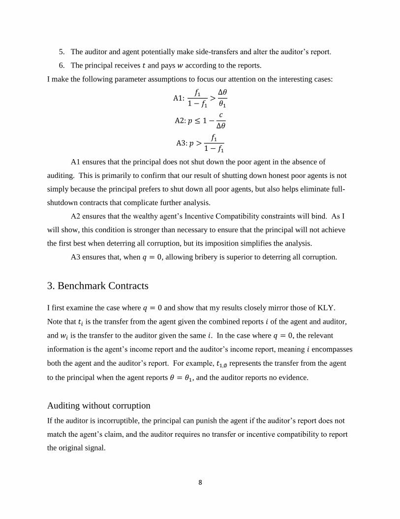
I make the following parameter assumptions to focus our attention on the interesting cases:

A1: 𝑓1

1 − 𝑓1>

Δ𝜃

𝜃1

A2: 𝑝 ≤ 1 −𝑐

Δ𝜃

A3: 𝑝 >𝑓1

1 − 𝑓1

A1 ensures that the principal does not shut down the poor agent in the absence of

auditing. This is primarily to confirm that our result of shutting down honest poor agents is not

simply because the principal prefers to shut down all poor agents, but also helps eliminate full-

shutdown contracts that complicate further analysis.

A2 ensures that the wealthy agent’s Incentive Compatibility constraints will bind. As I

will show, this condition is stronger than necessary to ensure that the principal will not achieve

the first best when deterring all corruption, but its imposition simplifies the analysis.

A3 ensures that, when 𝑞 = 0, allowing bribery is superior to deterring all corruption.

3. Benchmark Contracts

I first examine the case where 𝑞 = 0 and show that my results closely mirror those of KLY.

Note that 𝑡𝑖 is the transfer from the agent given the combined reports 𝑖 of the agent and auditor,

and 𝑤𝑖 is the transfer to the auditor given the same 𝑖. In the case where 𝑞 = 0, the relevant

information is the agent’s income report and the auditor’s income report, meaning 𝑖 encompasses

both the agent and the auditor’s report. For example, 𝑡1,∅ represents the transfer from the agent

to the principal when the agent reports 𝜃 = 𝜃1, and the auditor reports no evidence.

Auditing without corruption

If the auditor is incorruptible, the principal can punish the agent if the auditor’s report does not

match the agent’s claim, and the auditor requires no transfer or incentive compatibility to report

the original signal.

9

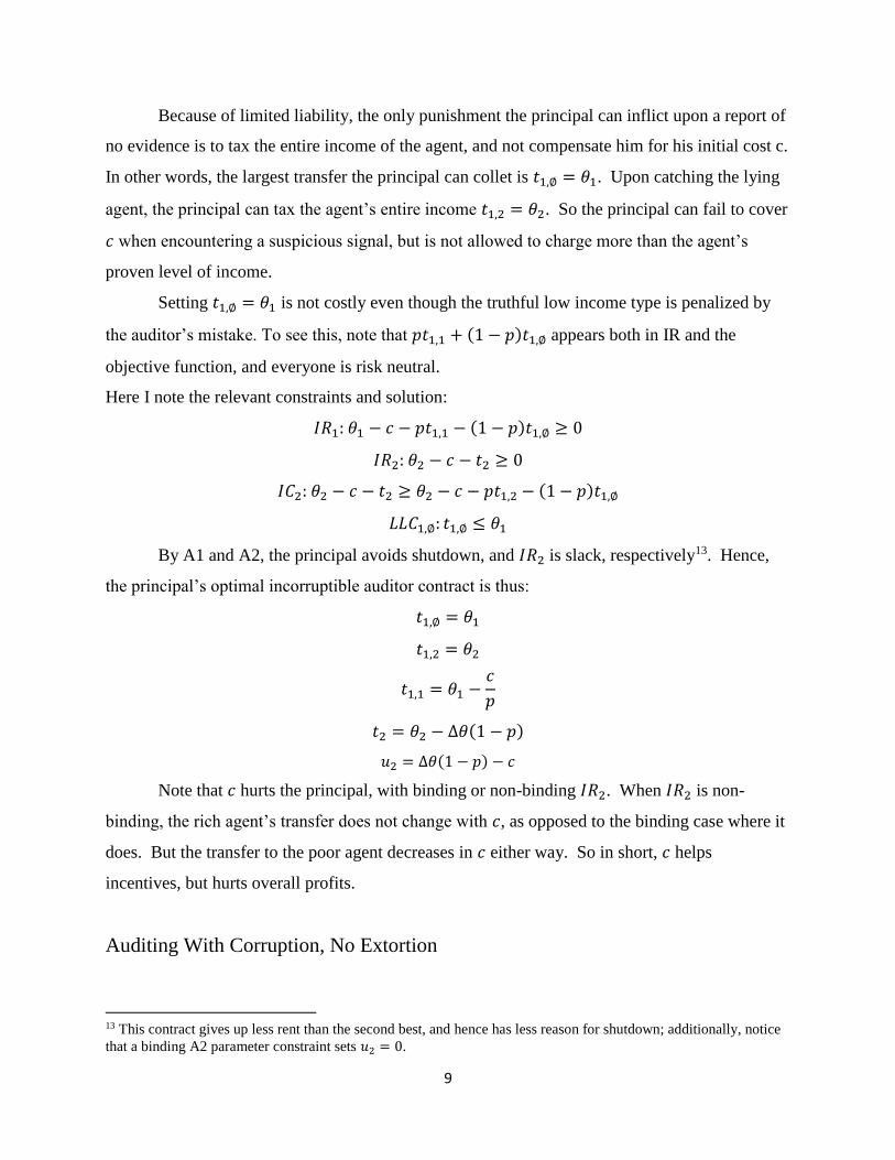
Because of limited liability, the only punishment the principal can inflict upon a report of

no evidence is to tax the entire income of the agent, and not compensate him for his initial cost c.

In other words, the largest transfer the principal can collet is 𝑡1,∅ = 𝜃1. Upon catching the lying

agent, the principal can tax the agent’s entire income 𝑡1,2 = 𝜃2. So the principal can fail to cover

𝑐 when encountering a suspicious signal, but is not allowed to charge more than the agent’s

proven level of income.

Setting 𝑡1,∅ = 𝜃1 is not costly even though the truthful low income type is penalized by

the auditor’s mistake. To see this, note that 𝑝𝑡1,1 + (1 − 𝑝)𝑡1,∅ appears both in IR and the

objective function, and everyone is risk neutral.

Here I note the relevant constraints and solution:

𝐼𝑅1: 𝜃1 − 𝑐 − 𝑝𝑡1,1 − (1 − 𝑝)𝑡1,∅ ≥ 0

𝐼𝑅2: 𝜃2 − 𝑐 − 𝑡2 ≥ 0

𝐼𝐶2: 𝜃2 − 𝑐 − 𝑡2 ≥ 𝜃2 − 𝑐 − 𝑝𝑡1,2 − (1 − 𝑝)𝑡1,∅

𝐿𝐿𝐶1,∅: 𝑡1,∅ ≤ 𝜃1

By A1 and A2, the principal avoids shutdown, and 𝐼𝑅2 is slack, respectively13. Hence,

the principal’s optimal incorruptible auditor contract is thus:

𝑡1,∅ = 𝜃1

𝑡1,2 = 𝜃2

𝑡1,1 = 𝜃1 −𝑐

𝑝

𝑡2 = 𝜃2 − Δ𝜃(1 − 𝑝)

𝑢2 = Δ𝜃(1 − 𝑝) − 𝑐

Note that 𝑐 hurts the principal, with binding or non-binding 𝐼𝑅2. When 𝐼𝑅2 is non-

binding, the rich agent’s transfer does not change with 𝑐, as opposed to the binding case where it

does. But the transfer to the poor agent decreases in 𝑐 either way. So in short, 𝑐 helps

incentives, but hurts overall profits.

Auditing With Corruption, No Extortion

13 This contract gives up less rent than the second best, and hence has less reason for shutdown; additionally, notice

that a binding A2 parameter constraint sets 𝑢2 = 0.

10

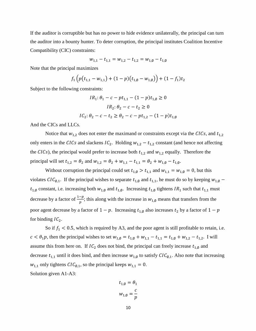
If the auditor is corruptible but has no power to hide evidence unilaterally, the principal can turn

the auditor into a bounty hunter. To deter corruption, the principal institutes Coalition Incentive

Compatibility (CIC) constraints:

𝑤1,1 − 𝑡1,1 = 𝑤1,2 − 𝑡1,2 = 𝑤1,∅ − 𝑡1,∅

Note that the principal maximizes

𝑓1 (𝑝(𝑡1,1 − 𝑤1,1) + (1 − 𝑝)(𝑡1,∅ − 𝑤1,∅)) + (1 − 𝑓1)𝑡2

Subject to the following constraints:

𝐼𝑅1: 𝜃1 − 𝑐 − 𝑝𝑡1,1 − (1 − 𝑝)𝑡1,∅ ≥ 0

𝐼𝑅2: 𝜃2 − 𝑐 − 𝑡2 ≥ 0

𝐼𝐶2: 𝜃2 − 𝑐 − 𝑡2 ≥ 𝜃2 − 𝑐 − 𝑝𝑡1,2 − (1 − 𝑝)𝑡1,∅

And the CICs and LLCs.

Notice that 𝑤1,2 does not enter the maximand or constraints except via the 𝐶𝐼𝐶𝑠, and 𝑡1,2

only enters in the 𝐶𝐼𝐶𝑠 and slackens 𝐼𝐶2. Holding 𝑤1,2 − 𝑡1,2 constant (and hence not affecting

the 𝐶𝐼𝐶𝑠), the principal would prefer to increase both 𝑡1,2 and 𝑤1,2 equally. Therefore the

principal will set 𝑡1,2 = 𝜃2 and 𝑤1,2 = 𝜃2 + 𝑤1,1 − 𝑡1,1 = 𝜃2 + 𝑤1,∅ − 𝑡1,∅.

Without corruption the principal could set 𝑡1,∅ > 𝑡1,1 and 𝑤1,1 = 𝑤1,∅ = 0, but this

violates 𝐶𝐼𝐶∅,1. If the principal wishes to separate 𝑡1,∅ and 𝑡1,1, he must do so by keeping 𝑤1,∅ −

𝑡1,∅ constant, i.e. increasing both 𝑤1,∅ and 𝑡1,∅. Increasing 𝑡1,∅ tightens 𝐼𝑅1 such that 𝑡1,1 must

decrease by a factor of 1−𝑝

𝑝; this along with the increase in 𝑤1,∅ means that transfers from the

poor agent decrease by a factor of 1 − 𝑝. Increasing 𝑡1,∅ also increases 𝑡2 by a factor of 1 − 𝑝

for binding 𝐼𝐶2.

So if 𝑓1 < 0.5, which is required by A3, and the poor agent is still profitable to retain, i.e.

𝑐 < 𝜃1𝑝, then the principal wishes to set 𝑤1,∅ = 𝑡1,∅ + 𝑤1,1 − 𝑡1,1 = 𝑡1,∅ + 𝑤1,2 − 𝑡1,2. I will

assume this from here on. If 𝐼𝐶2 does not bind, the principal can freely increase 𝑡1,∅ and

decrease 𝑡1,1 until it does bind, and then increase 𝑤1,∅ to satisfy 𝐶𝐼𝐶∅,1. Also note that increasing

𝑤1,1 only tightens 𝐶𝐼𝐶∅,1, so the principal keeps 𝑤1,1 = 0.

Solution given A1-A3:

𝑡1,∅ = 𝜃1

𝑤1,∅ =𝑐

𝑝

11

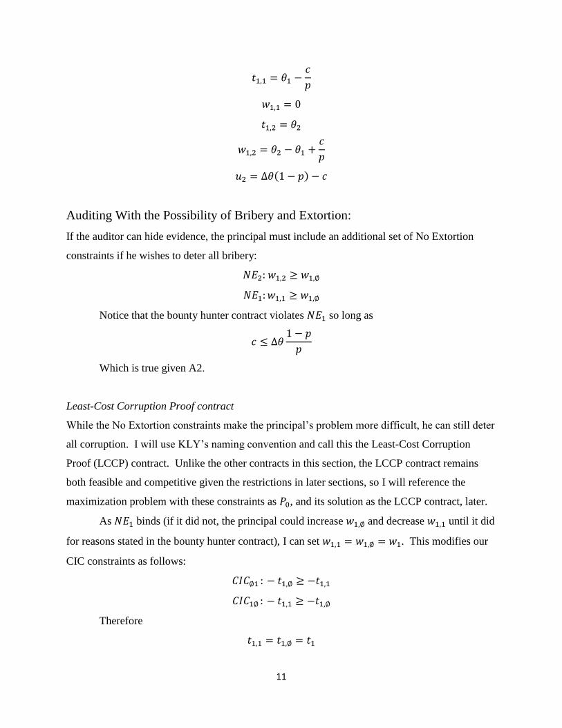
𝑡1,1 = 𝜃1 −𝑐

𝑝

𝑤1,1 = 0

𝑡1,2 = 𝜃2

𝑤1,2 = 𝜃2 − 𝜃1 +𝑐

𝑝

𝑢2 = Δ𝜃(1 − 𝑝) − 𝑐

Auditing With the Possibility of Bribery and Extortion:

If the auditor can hide evidence, the principal must include an additional set of No Extortion

constraints if he wishes to deter all bribery:

𝑁𝐸2: 𝑤1,2 ≥ 𝑤1,∅

𝑁𝐸1: 𝑤1,1 ≥ 𝑤1,∅

Notice that the bounty hunter contract violates 𝑁𝐸1 so long as

𝑐 ≤ Δ𝜃1 − 𝑝

𝑝

Which is true given A2.

Least-Cost Corruption Proof contract

While the No Extortion constraints make the principal’s problem more difficult, he can still deter

all corruption. I will use KLY’s naming convention and call this the Least-Cost Corruption

Proof (LCCP) contract. Unlike the other contracts in this section, the LCCP contract remains

both feasible and competitive given the restrictions in later sections, so I will reference the

maximization problem with these constraints as 𝑃0, and its solution as the LCCP contract, later.

As 𝑁𝐸1 binds (if it did not, the principal could increase 𝑤1,∅ and decrease 𝑤1,1 until it did

for reasons stated in the bounty hunter contract), I can set 𝑤1,1 = 𝑤1,∅ = 𝑤1. This modifies our

CIC constraints as follows:

𝐶𝐼𝐶∅1 : − 𝑡1,∅ ≥ −𝑡1,1

𝐶𝐼𝐶1∅ : − 𝑡1,1 ≥ −𝑡1,∅

Therefore

𝑡1,1 = 𝑡1,∅ = 𝑡1

12

Note that the principal can still set 𝑤12 = 𝑡12 + 𝑤1 − 𝑡1 to satisfy the proper CICs

without violating NE, as the auditor cannot fake evidence; he can only hide it. In fact, increasing

𝑤12 causes 𝑁𝐸2 to go slack. With this in mind, the principal will set 𝑡1,2 = 𝜃2 and 𝑤1,2 = 𝜃2 +

𝑤1 − 𝑡1.

Increasing 𝑤1 decreases the net transfer to the principal, tightens 𝐶𝐼𝐶21 and 𝐶𝐼𝐶2∅, and

otherwise does nothing. Therefore the principal will set 𝑤1 = 0. Knowing this I can derive the

full solution from the binding constraints:

𝐼𝑅1: 𝜃1 − 𝑡1 − 𝑐 ≥ 0

𝐼𝑅2: 𝜃2 − 𝑐 − 𝑡2 ≥ 0

𝐼𝐶2: 𝜃2 − 𝑐 − 𝑡2 ≥ 𝜃2(1 − 𝑝) − 𝑐 − (1 − 𝑝)𝑡1

If 𝐼𝑅2 is slack,

𝑢2 = Δ𝜃(1 − 𝑝) − 𝑝𝑐

𝜃2 − 𝑐 − 𝑡2 = Δ𝜃(1 − 𝑝) − 𝑝𝑐

𝑡2 = 𝜃2 − Δ𝜃(1 − 𝑝) − (1 − 𝑝)𝑐

This occurs when 𝑐 ≤ Δ𝜃1−𝑝

𝑝, which is satisfied by A2. The principal can achieve the

first best while deterring all corruption (replicating the bounty hunter contract) when 𝑐 ≥ Δ𝜃1−𝑝

𝑝

Full solution for ≤ Δ𝜃1−𝑝

𝑝 14:

𝑡2 = 𝜃2 − Δ𝜃(1 − 𝑝) − (1 − 𝑝)𝑐

𝑡1,1 = 𝑡1,∅ = 𝑡1 = 𝜃1 − 𝑐

𝑤1,1 = 𝑤1,∅ = 𝑤1 = 0

𝑡1,2 = 𝜃2

𝑤1,2 = Δ𝜃 + 𝑐

Agent-Auditor Side Contracting

The agent’s bargaining power is represented by 𝜆, 0 < 𝜆 < 1 in the Nash bargaining solution. If

the net transfer from the auditor-agent coalition to the principal before report-alteration is 𝑇𝑖 =

𝑡𝑖 − 𝑤𝑖, and the net transfer from the coalition to the principal after report-alteration is 𝑇𝑗 = 𝑡𝑗 −

𝑤𝑗 < 𝑡𝑖 − 𝑤𝑖, then the agent collaborates with the auditor and effectively pays a transfer 𝑡𝑖′ =

14 Note that this is the necessary condition for LCCP not to replicate the first best, as opposed to A2.

13

𝑡𝑖 + 𝜆 ((𝑡𝑗 − 𝑤𝑗) − (𝑡𝑖 − 𝑤𝑖)) = (1 − 𝜆)𝑡𝑖 + 𝜆 (𝑡𝑗 − (𝑤𝑗 − 𝑤𝑖)). If the signal is already the

most profitable for the coalition (as is the case in LCCP), 𝑡𝑖′ = 𝑡𝑖. This is derived in Appendix A.

Note that this derivation applies to any strategic agent when 𝑞 > 0 as well.

Allowing Extortion is Never Optimal

See Appendix B for the full proof. Intuitively, when extortion is allowed, the agent obtains the

same payoffs as in the LCCP contract for various signals, but the auditor receives rent. This rent

makes any extortion-allowing contract more costly than the LCCP contract at the same levels of

effort, so the extortion-allowing contract is suboptimal. Extortion imposes an expected penalty

for working instead of shirking, whereas bribery still imposes an expected penalty for shirking.

Therefore one might expect a contract to allow bribery, but never extortion. From now on I will

re-introduce the NE constraints.

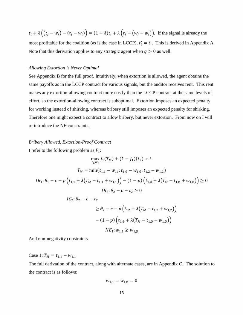
Bribery Allowed, Extortion-Proof Contract

I refer to the following problem as 𝑃1:

max𝑡𝑖,𝑤𝑖

𝑓1(𝑇𝑀) + (1 − 𝑓1)(𝑡2) 𝑠. 𝑡.

𝑇𝑀 = min(𝑡1,1 − 𝑤11; 𝑡1,∅ − 𝑤1,∅; 𝑡1,2 − 𝑤1,2)

𝐼𝑅1: 𝜃1 − 𝑐 − 𝑝 (𝑡1,1 + 𝜆(𝑇𝑀 − 𝑡1,1 + 𝑤1,1)) − (1 − 𝑝) (𝑡1,∅ + 𝜆(𝑇𝑀 − 𝑡1,∅ + 𝑤1,∅)) ≥ 0

𝐼𝑅2: 𝜃2 − 𝑐 − 𝑡2 ≥ 0

𝐼𝐶2: 𝜃2 − 𝑐 − 𝑡2

≥ 𝜃2 − 𝑐 − 𝑝 (𝑡12 + 𝜆(𝑇𝑀 − 𝑡1,2 + 𝑤1,2))

− (1 − 𝑝) (𝑡1,∅ + 𝜆(𝑇𝑀 − 𝑡1,∅ + 𝑤1,∅))

𝑁𝐸1: 𝑤1,1 ≥ 𝑤1,∅

And non-negativity constraints

Case 1: 𝑇𝑀 = 𝑡1,1 − 𝑤1,1

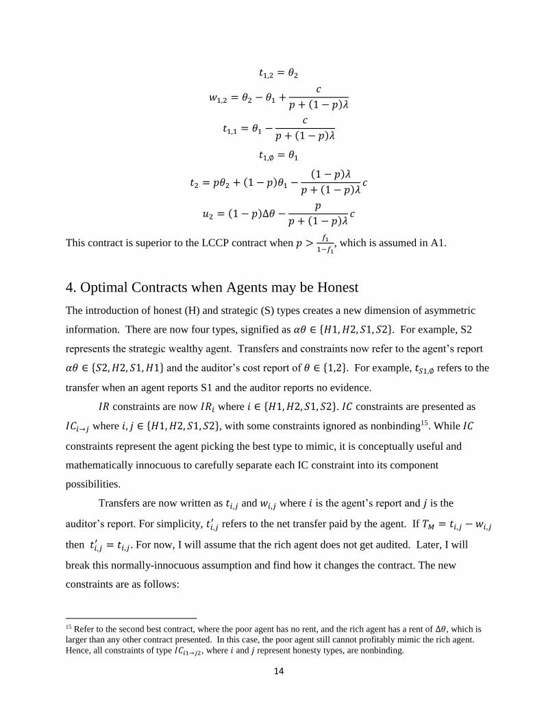
The full derivation of the contract, along with alternate cases, are in Appendix C. The solution to

the contract is as follows:

𝑤1,1 = 𝑤1,∅ = 0

14

𝑡1,2 = 𝜃2

𝑤1,2 = 𝜃2 − 𝜃1 +𝑐

𝑝 + (1 − 𝑝)𝜆

𝑡1,1 = 𝜃1 −𝑐

𝑝 + (1 − 𝑝)𝜆

𝑡1,∅ = 𝜃1

𝑡2 = 𝑝𝜃2 + (1 − 𝑝)𝜃1 −(1 − 𝑝)𝜆

𝑝 + (1 − 𝑝)𝜆𝑐

𝑢2 = (1 − 𝑝)Δ𝜃 −𝑝

𝑝 + (1 − 𝑝)𝜆𝑐

This contract is superior to the LCCP contract when 𝑝 >𝑓1

1−𝑓1, which is assumed in A1.

4. Optimal Contracts when Agents may be Honest

The introduction of honest (H) and strategic (S) types creates a new dimension of asymmetric

information. There are now four types, signified as 𝛼𝜃 ∈ {𝐻1, 𝐻2, 𝑆1, 𝑆2}. For example, S2

represents the strategic wealthy agent. Transfers and constraints now refer to the agent’s report

𝛼𝜃 ∈ {𝑆2, 𝐻2, 𝑆1, 𝐻1} and the auditor’s cost report of 𝜃 ∈ {1,2}. For example, 𝑡𝑆1,∅ refers to the

transfer when an agent reports S1 and the auditor reports no evidence.

𝐼𝑅 constraints are now 𝐼𝑅𝑖 where 𝑖 ∈ {𝐻1, 𝐻2, 𝑆1, 𝑆2}. 𝐼𝐶 constraints are presented as

𝐼𝐶𝑖→𝑗 where 𝑖, 𝑗 ∈ {𝐻1, 𝐻2, 𝑆1, 𝑆2}, with some constraints ignored as nonbinding15. While 𝐼𝐶

constraints represent the agent picking the best type to mimic, it is conceptually useful and

mathematically innocuous to carefully separate each IC constraint into its component

possibilities.

Transfers are now written as 𝑡𝑖,𝑗 and 𝑤𝑖,𝑗 where 𝑖 is the agent’s report and 𝑗 is the

auditor’s report. For simplicity, 𝑡𝑖,𝑗′ refers to the net transfer paid by the agent. If 𝑇𝑀 = 𝑡𝑖,𝑗 − 𝑤𝑖,𝑗

then 𝑡𝑖,𝑗′ = 𝑡𝑖,𝑗. For now, I will assume that the rich agent does not get audited. Later, I will

break this normally-innocuous assumption and find how it changes the contract. The new

constraints are as follows:

15 Refer to the second best contract, where the poor agent has no rent, and the rich agent has a rent of Δ𝜃, which is

larger than any other contract presented. In this case, the poor agent still cannot profitably mimic the rich agent.

Hence, all constraints of type 𝐼𝐶𝑖1→𝑗2, where 𝑖 and 𝑗 represent honesty types, are nonbinding.

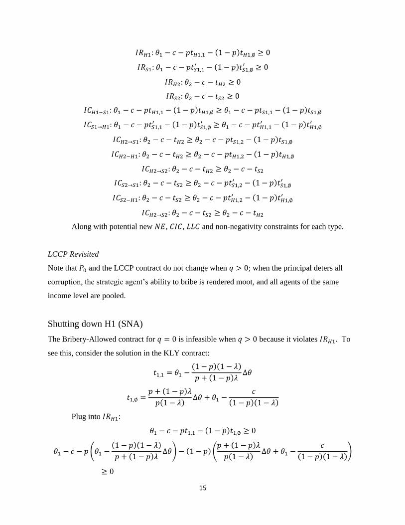
15

𝐼𝑅𝐻1: 𝜃1 − 𝑐 − 𝑝𝑡𝐻1,1 − (1 − 𝑝)𝑡𝐻1,∅ ≥ 0

𝐼𝑅𝑆1: 𝜃1 − 𝑐 − 𝑝𝑡𝑆1,1′ − (1 − 𝑝)𝑡𝑆1,∅

′ ≥ 0

𝐼𝑅𝐻2: 𝜃2 − 𝑐 − 𝑡𝐻2 ≥ 0

𝐼𝑅𝑆2: 𝜃2 − 𝑐 − 𝑡𝑆2 ≥ 0

𝐼𝐶𝐻1−𝑆1: 𝜃1 − 𝑐 − 𝑝𝑡𝐻1,1 − (1 − 𝑝)𝑡𝐻1,∅ ≥ 𝜃1 − 𝑐 − 𝑝𝑡𝑆1,1 − (1 − 𝑝)𝑡𝑆1,∅

𝐼𝐶𝑆1→𝐻1: 𝜃1 − 𝑐 − 𝑝𝑡𝑆1,1′ − (1 − 𝑝)𝑡𝑆1,∅

′ ≥ 𝜃1 − 𝑐 − 𝑝𝑡𝐻1,1′ − (1 − 𝑝)𝑡𝐻1,∅

′

𝐼𝐶𝐻2→𝑆1: 𝜃2 − 𝑐 − 𝑡𝐻2 ≥ 𝜃2 − 𝑐 − 𝑝𝑡𝑆1,2 − (1 − 𝑝)𝑡𝑆1,∅

𝐼𝐶𝐻2−𝐻1: 𝜃2 − 𝑐 − 𝑡𝐻2 ≥ 𝜃2 − 𝑐 − 𝑝𝑡𝐻1,2 − (1 − 𝑝)𝑡𝐻1,∅

𝐼𝐶𝐻2→𝑆2: 𝜃2 − 𝑐 − 𝑡𝐻2 ≥ 𝜃2 − 𝑐 − 𝑡𝑆2

𝐼𝐶𝑆2→𝑆1: 𝜃2 − 𝑐 − 𝑡𝑆2 ≥ 𝜃2 − 𝑐 − 𝑝𝑡𝑆1,2′ − (1 − 𝑝)𝑡𝑆1,∅

′

𝐼𝐶𝑆2−𝐻1: 𝜃2 − 𝑐 − 𝑡𝑆2 ≥ 𝜃2 − 𝑐 − 𝑝𝑡𝐻1,2′ − (1 − 𝑝)𝑡𝐻1,∅

′

𝐼𝐶𝐻2→𝑆2: 𝜃2 − 𝑐 − 𝑡𝑆2 ≥ 𝜃2 − 𝑐 − 𝑡𝐻2

Along with potential new 𝑁𝐸, 𝐶𝐼𝐶, 𝐿𝐿𝐶 and non-negativity constraints for each type.

LCCP Revisited

Note that 𝑃0 and the LCCP contract do not change when 𝑞 > 0; when the principal deters all

corruption, the strategic agent’s ability to bribe is rendered moot, and all agents of the same

income level are pooled.

Shutting down H1 (SNA)

The Bribery-Allowed contract for 𝑞 = 0 is infeasible when 𝑞 > 0 because it violates 𝐼𝑅𝐻1. To

see this, consider the solution in the KLY contract:

𝑡1,1 = 𝜃1 −(1 − 𝑝)(1 − 𝜆)

𝑝 + (1 − 𝑝)𝜆Δ𝜃

𝑡1,∅ =𝑝 + (1 − 𝑝)𝜆

𝑝(1 − 𝜆)Δ𝜃 + 𝜃1 −

𝑐

(1 − 𝑝)(1 − 𝜆)

Plug into 𝐼𝑅𝐻1:

𝜃1 − 𝑐 − 𝑝𝑡1,1 − (1 − 𝑝)𝑡1,∅ ≥ 0

𝜃1 − 𝑐 − 𝑝 (𝜃1 −(1 − 𝑝)(1 − 𝜆)

𝑝 + (1 − 𝑝)𝜆Δ𝜃) − (1 − 𝑝) (

𝑝 + (1 − 𝑝)𝜆

𝑝(1 − 𝜆)Δ𝜃 + 𝜃1 −

𝑐

(1 − 𝑝)(1 − 𝜆))

≥ 0

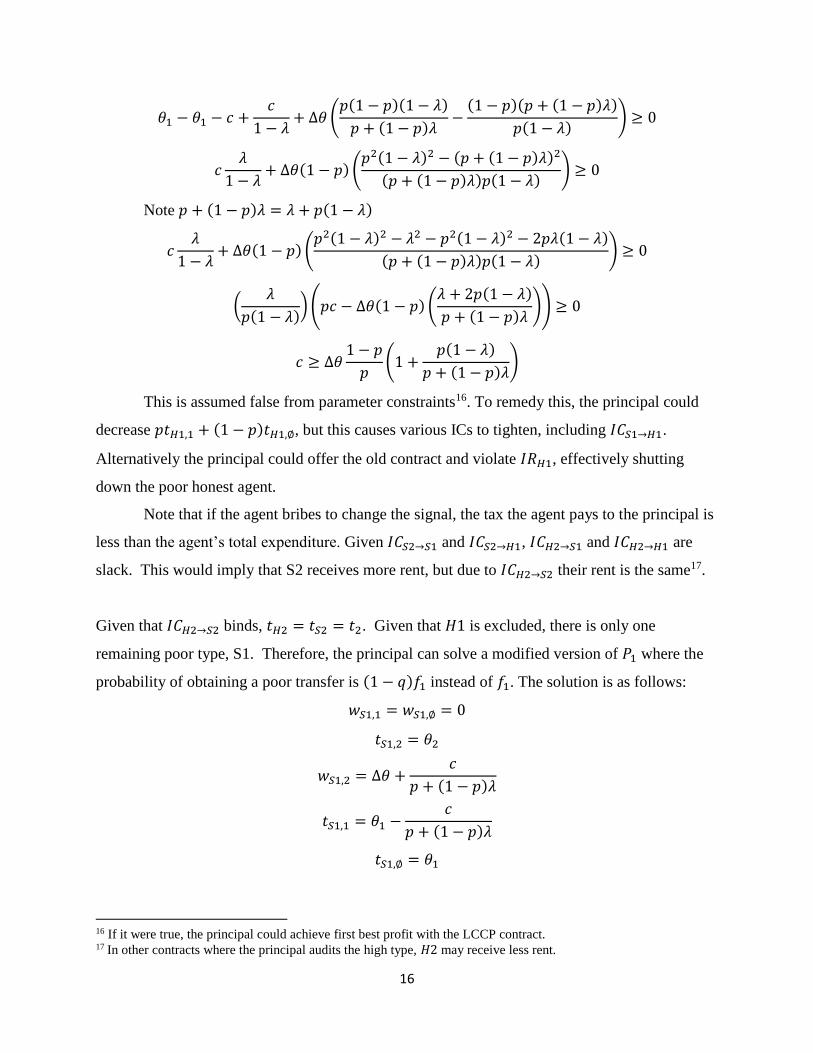
16

𝜃1 − 𝜃1 − 𝑐 +𝑐

1 − 𝜆+ Δ𝜃 (

𝑝(1 − 𝑝)(1 − 𝜆)

𝑝 + (1 − 𝑝)𝜆−

(1 − 𝑝)(𝑝 + (1 − 𝑝)𝜆)

𝑝(1 − 𝜆)) ≥ 0

𝑐𝜆

1 − 𝜆+ Δ𝜃(1 − 𝑝) (

𝑝2(1 − 𝜆)2 − (𝑝 + (1 − 𝑝)𝜆)2

(𝑝 + (1 − 𝑝)𝜆)𝑝(1 − 𝜆)) ≥ 0

Note 𝑝 + (1 − 𝑝)𝜆 = 𝜆 + 𝑝(1 − 𝜆)

𝑐𝜆

1 − 𝜆+ Δ𝜃(1 − 𝑝) (

𝑝2(1 − 𝜆)2 − 𝜆2 − 𝑝2(1 − 𝜆)2 − 2𝑝𝜆(1 − 𝜆)

(𝑝 + (1 − 𝑝)𝜆)𝑝(1 − 𝜆)) ≥ 0

(𝜆

𝑝(1 − 𝜆)) (𝑝𝑐 − Δ𝜃(1 − 𝑝) (

𝜆 + 2𝑝(1 − 𝜆)

𝑝 + (1 − 𝑝)𝜆)) ≥ 0

𝑐 ≥ Δ𝜃1 − 𝑝

𝑝(1 +

𝑝(1 − 𝜆)

𝑝 + (1 − 𝑝)𝜆)

This is assumed false from parameter constraints16. To remedy this, the principal could

decrease 𝑝𝑡𝐻1,1 + (1 − 𝑝)𝑡𝐻1,∅, but this causes various ICs to tighten, including 𝐼𝐶𝑆1→𝐻1.

Alternatively the principal could offer the old contract and violate 𝐼𝑅𝐻1, effectively shutting

down the poor honest agent.

Note that if the agent bribes to change the signal, the tax the agent pays to the principal is

less than the agent’s total expenditure. Given 𝐼𝐶𝑆2→𝑆1 and 𝐼𝐶𝑆2→𝐻1, 𝐼𝐶𝐻2→𝑆1 and 𝐼𝐶𝐻2→𝐻1 are

slack. This would imply that S2 receives more rent, but due to 𝐼𝐶𝐻2→𝑆2 their rent is the same17.

Given that 𝐼𝐶𝐻2→𝑆2 binds, 𝑡𝐻2 = 𝑡𝑆2 = 𝑡2. Given that 𝐻1 is excluded, there is only one

remaining poor type, S1. Therefore, the principal can solve a modified version of 𝑃1 where the

probability of obtaining a poor transfer is (1 − 𝑞)𝑓1 instead of 𝑓1. The solution is as follows:

𝑤𝑆1,1 = 𝑤𝑆1,∅ = 0

𝑡𝑆1,2 = 𝜃2

𝑤𝑆1,2 = Δ𝜃 +𝑐

𝑝 + (1 − 𝑝)𝜆

𝑡𝑆1,1 = 𝜃1 −𝑐

𝑝 + (1 − 𝑝)𝜆

𝑡𝑆1,∅ = 𝜃1

16 If it were true, the principal could achieve first best profit with the LCCP contract. 17 In other contracts where the principal audits the high type, 𝐻2 may receive less rent.

17

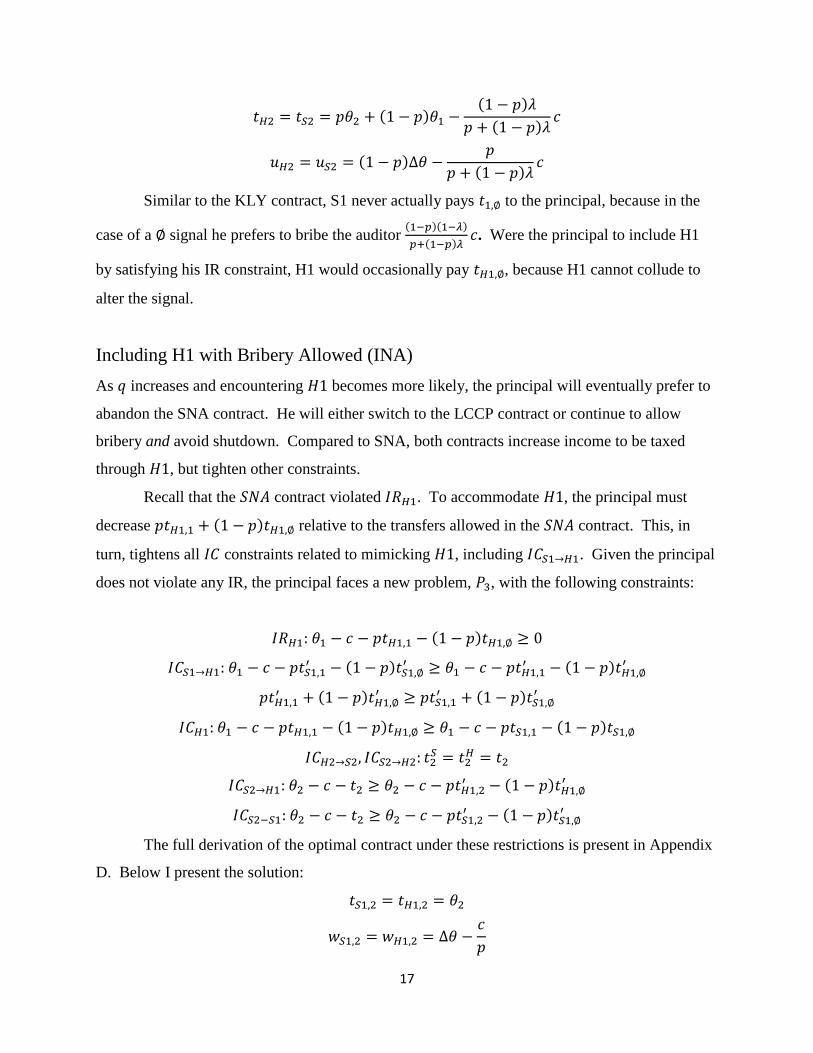
𝑡𝐻2 = 𝑡𝑆2 = 𝑝𝜃2 + (1 − 𝑝)𝜃1 −(1 − 𝑝)𝜆

𝑝 + (1 − 𝑝)𝜆𝑐

𝑢𝐻2 = 𝑢𝑆2 = (1 − 𝑝)Δ𝜃 −𝑝

𝑝 + (1 − 𝑝)𝜆𝑐

Similar to the KLY contract, S1 never actually pays 𝑡1,∅ to the principal, because in the

case of a ∅ signal he prefers to bribe the auditor (1−𝑝)(1−𝜆)

𝑝+(1−𝑝)𝜆𝑐. Were the principal to include H1

by satisfying his IR constraint, H1 would occasionally pay 𝑡𝐻1,∅, because H1 cannot collude to

alter the signal.

Including H1 with Bribery Allowed (INA)

As 𝑞 increases and encountering 𝐻1 becomes more likely, the principal will eventually prefer to

abandon the SNA contract. He will either switch to the LCCP contract or continue to allow

bribery and avoid shutdown. Compared to SNA, both contracts increase income to be taxed

through 𝐻1, but tighten other constraints.

Recall that the 𝑆𝑁𝐴 contract violated 𝐼𝑅𝐻1. To accommodate 𝐻1, the principal must

decrease 𝑝𝑡𝐻1,1 + (1 − 𝑝)𝑡𝐻1,∅ relative to the transfers allowed in the 𝑆𝑁𝐴 contract. This, in

turn, tightens all 𝐼𝐶 constraints related to mimicking 𝐻1, including 𝐼𝐶𝑆1→𝐻1. Given the principal

does not violate any IR, the principal faces a new problem, 𝑃3, with the following constraints:

𝐼𝑅𝐻1: 𝜃1 − 𝑐 − 𝑝𝑡𝐻1,1 − (1 − 𝑝)𝑡𝐻1,∅ ≥ 0

𝐼𝐶𝑆1→𝐻1: 𝜃1 − 𝑐 − 𝑝𝑡𝑆1,1′ − (1 − 𝑝)𝑡𝑆1,∅

′ ≥ 𝜃1 − 𝑐 − 𝑝𝑡𝐻1,1′ − (1 − 𝑝)𝑡𝐻1,∅

′

𝑝𝑡𝐻1,1′ + (1 − 𝑝)𝑡𝐻1,∅

′ ≥ 𝑝𝑡𝑆1,1′ + (1 − 𝑝)𝑡𝑆1,∅

′

𝐼𝐶𝐻1: 𝜃1 − 𝑐 − 𝑝𝑡𝐻1,1 − (1 − 𝑝)𝑡𝐻1,∅ ≥ 𝜃1 − 𝑐 − 𝑝𝑡𝑆1,1 − (1 − 𝑝)𝑡𝑆1,∅

𝐼𝐶𝐻2→𝑆2, 𝐼𝐶𝑆2→𝐻2: 𝑡2𝑆 = 𝑡2

𝐻 = 𝑡2

𝐼𝐶𝑆2→𝐻1: 𝜃2 − 𝑐 − 𝑡2 ≥ 𝜃2 − 𝑐 − 𝑝𝑡𝐻1,2′ − (1 − 𝑝)𝑡𝐻1,∅

′

𝐼𝐶𝑆2−𝑆1: 𝜃2 − 𝑐 − 𝑡2 ≥ 𝜃2 − 𝑐 − 𝑝𝑡𝑆1,2′ − (1 − 𝑝)𝑡𝑆1,∅

′

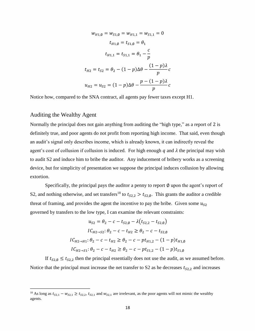
The full derivation of the optimal contract under these restrictions is present in Appendix

D. Below I present the solution:

𝑡𝑆1,2 = 𝑡𝐻1,2 = 𝜃2

𝑤𝑆1,2 = 𝑤𝐻1,2 = Δ𝜃 −𝑐

𝑝

18

𝑤𝐻1,∅ = 𝑤𝑆1,∅ = 𝑤𝐻1,1 = 𝑤𝑆1,1 = 0

𝑡𝐻1,∅ = 𝑡𝑆1,∅ = 𝜃1

𝑡𝐻1,1 = 𝑡𝑆1,1 = 𝜃1 −𝑐

𝑝

𝑡𝐻2 = 𝑡𝑆2 = 𝜃2 − (1 − 𝑝)Δ𝜃 −(1 − 𝑝)𝜆

𝑝𝑐

𝑢𝐻2 = 𝑢𝑆2 = (1 − 𝑝)Δ𝜃 −𝑝 − (1 − 𝑝)𝜆

𝑝𝑐

Notice how, compared to the SNA contract, all agents pay fewer taxes except H1.

Auditing the Wealthy Agent

Normally the principal does not gain anything from auditing the “high type,” as a report of 2 is

definitely true, and poor agents do not profit from reporting high income. That said, even though

an audit’s signal only describes income, which is already known, it can indirectly reveal the

agent’s cost of collusion if collusion is induced. For high enough 𝑞 and 𝜆 the principal may wish

to audit S2 and induce him to bribe the auditor. Any inducement of bribery works as a screening

device, but for simplicity of presentation we suppose the principal induces collusion by allowing

extortion.

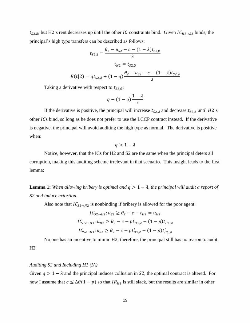
Specifically, the principal pays the auditor a penny to report ∅ upon the agent’s report of

S2, and nothing otherwise, and set transfers18 to 𝑡𝑆2,2 > 𝑡𝑆2,∅. This grants the auditor a credible

threat of framing, and provides the agent the incentive to pay the bribe. Given some 𝑢𝑆2

governed by transfers to the low type, I can examine the relevant constraints:

𝑢𝑆2 = 𝜃2 − 𝑐 − 𝑡𝑆2,∅ − 𝜆(𝑡𝑆2,2 − 𝑡𝑆2,∅)

𝐼𝐶𝐻2→𝑆2: 𝜃2 − 𝑐 − 𝑡𝐻2 ≥ 𝜃2 − 𝑐 − 𝑡𝑆2,∅

𝐼𝐶𝐻2→𝐻1: 𝜃2 − 𝑐 − 𝑡𝐻2 ≥ 𝜃2 − 𝑐 − 𝑝𝑡𝐻1,2 − (1 − 𝑝)𝑡𝐻1,∅

𝐼𝐶𝐻2→𝑆1: 𝜃2 − 𝑐 − 𝑡𝐻2 ≥ 𝜃2 − 𝑐 − 𝑝𝑡𝑆1,2 − (1 − 𝑝)𝑡𝑆1,∅

If 𝑡𝑆2,∅ ≤ 𝑡𝑆2,2 then the principal essentially does not use the audit, as we assumed before.

Notice that the principal must increase the net transfer to S2 as he decreases 𝑡𝑆2,2 and increases

18 As long as 𝑡𝑆2,1 − 𝑤𝑆2,1 ≥ 𝑡𝑆2,2, 𝑡𝑆2,1 and 𝑤𝑆2,1 are irrelevant, as the poor agents will not mimic the wealthy

agents.

19

𝑡𝑆2,∅, but H2’s rent decreases up until the other 𝐼𝐶 constraints bind. Given 𝐼𝐶𝐻2→𝑆2 binds, the

principal’s high type transfers can be described as follows:

𝑡𝑆2,2 =𝜃2 − 𝑢𝑆2 − 𝑐 − (1 − 𝜆)𝑡𝑆2,∅

𝜆

𝑡𝐻2 = 𝑡𝑆2,∅

𝐸(𝑡|2) = 𝑞𝑡𝑆2,∅ + (1 − 𝑞)𝜃2 − 𝑢𝑆2 − 𝑐 − (1 − 𝜆)𝑡𝑆2,∅

𝜆

Taking a derivative with respect to 𝑡𝑆2,∅:

𝑞 − (1 − 𝑞)1 − 𝜆

𝜆

If the derivative is positive, the principal will increase 𝑡𝑆2,∅ and decrease 𝑡𝑆2,2 until 𝐻2’s

other 𝐼𝐶s bind, so long as he does not prefer to use the LCCP contract instead. If the derivative

is negative, the principal will avoid auditing the high type as normal. The derivative is positive

when:

𝑞 > 1 − 𝜆

Notice, however, that the ICs for H2 and S2 are the same when the principal deters all

corruption, making this auditing scheme irrelevant in that scenario. This insight leads to the first

lemma:

Lemma 1: When allowing bribery is optimal and 𝑞 > 1 − 𝜆, the principal will audit a report of

S2 and induce extortion.

Also note that 𝐼𝐶𝑆2→𝐻2 is nonbinding if bribery is allowed for the poor agent:

𝐼𝐶𝑆2→𝐻2: 𝑢𝑆2 ≥ 𝜃2 − 𝑐 − 𝑡𝐻2 = 𝑢𝐻2

𝐼𝐶𝐻2→𝐻1: 𝑢𝐻2 ≥ 𝜃2 − 𝑐 − 𝑝𝑡𝐻1,2 − (1 − 𝑝)𝑡𝐻1,∅

𝐼𝐶𝑆2→𝐻1: 𝑢𝑆2 ≥ 𝜃2 − 𝑐 − 𝑝𝑡𝐻1,2′ − (1 − 𝑝)𝑡𝐻1,∅

′

No one has an incentive to mimic H2; therefore, the principal still has no reason to audit

H2.

Auditing S2 and Including H1 (IA)

Given 𝑞 > 1 − 𝜆 and the principal induces collusion in 𝑆2, the optimal contract is altered. For

now I assume that 𝑐 ≤ Δ𝜃(1 − 𝑝) so that 𝐼𝑅𝐻2 is still slack, but the results are similar in other

20

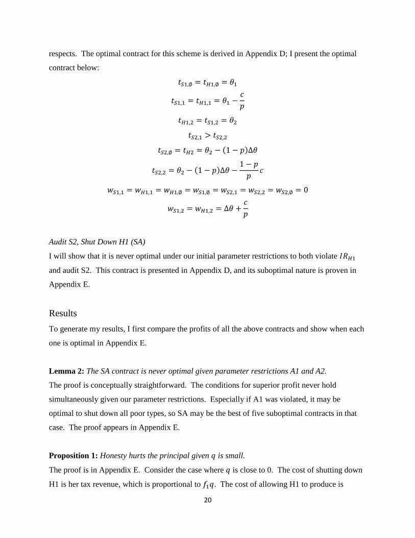
respects. The optimal contract for this scheme is derived in Appendix D; I present the optimal

contract below:

𝑡𝑆1,∅ = 𝑡𝐻1,∅ = 𝜃1

𝑡𝑆1,1 = 𝑡𝐻1,1 = 𝜃1 −𝑐

𝑝

𝑡𝐻1,2 = 𝑡𝑆1,2 = 𝜃2

𝑡𝑆2,1 > 𝑡𝑆2,2

𝑡𝑆2,∅ = 𝑡𝐻2 = 𝜃2 − (1 − 𝑝)Δ𝜃

𝑡𝑆2,2 = 𝜃2 − (1 − 𝑝)Δ𝜃 −1 − 𝑝

𝑝𝑐

𝑤𝑆1,1 = 𝑤𝐻1,1 = 𝑤𝐻1,∅ = 𝑤𝑆1,∅ = 𝑤𝑆2,1 = 𝑤𝑆2,2 = 𝑤𝑆2,∅ = 0

𝑤𝑆1,2 = 𝑤𝐻1,2 = Δ𝜃 +𝑐

𝑝

Audit S2, Shut Down H1 (SA)

I will show that it is never optimal under our initial parameter restrictions to both violate 𝐼𝑅𝐻1

and audit S2. This contract is presented in Appendix D, and its suboptimal nature is proven in

Appendix E.

Results

To generate my results, I first compare the profits of all the above contracts and show when each

one is optimal in Appendix E.

Lemma 2: The SA contract is never optimal given parameter restrictions A1 and A2.

The proof is conceptually straightforward. The conditions for superior profit never hold

simultaneously given our parameter restrictions. Especially if A1 was violated, it may be

optimal to shut down all poor types, so SA may be the best of five suboptimal contracts in that

case. The proof appears in Appendix E.

Proposition 1: Honesty hurts the principal given 𝑞 is small.

The proof is in Appendix E. Consider the case where 𝑞 is close to 0. The cost of shutting down

H1 is her tax revenue, which is proportional to 𝑓1𝑞. The cost of allowing H1 to produce is

21

granting rent to all other agents, which is roughly proportional to 1 − 𝑓1𝑞. Hence, for small 𝑞,

the principal will find it worthwhile to shut down H1 and emulate the KLY contract. While

small, clearly the cost of shutting down H1 increases in 𝑞, since no other aspect of the contract

changes, and more and more agents are shut down.

This represents the issue presented to a reformer in a corrupt society. There is an implied

dynamic effect of this model where honest individuals are continuously pushed out of corrupt

societies towards less corrupt ones. Conventionally negative norms of behavior may be enforced

for the sake of homogeneity. Hence, if policies do not generally increase the costs of corruption

and instead have a heterogeneous effect on individuals, the affected individuals may simply be

sorted out, at a cost to the home country.

Proposition 2: The principal will optimally audit S2 and induce extortion, given 𝑞 is large.

The proof takes the following steps:

1. Given Lemma 2, and given the IA contract is only valuable if bribery is allowed, the

principal’s optimal contract when inducing extortion for S2 is the IA contract.

2. The IA contract is superior for some �̲� < 𝑞 < 1, given Lemma 2 and the profit

comparison between IA and LCCP.

Step 1 is evident. For step 2, Lemma 1 shows that IA is superior to SNA and IA when 𝑞 >

1 − 𝜆. Additionally, IA is superior to LCCP when 𝑞 > 𝑓1 + (1 − 𝑓1)(1 − 𝑝). Define �̲� =

max(1 − 𝜆, 𝑓1 + (1 − 𝑓1)(1 − 𝑝) ). The IA contract is optimal when �̲� < 𝑞 < 1.

When most agents do not engage in corrupt behavior, the principal is more willing to pay

more to accommodate corrupt agents, so long as it maximizes honest revenue. In particular,

forcing strategic wealthy agents to engage in actual corruption to obtain their rents allows the

principal to screen wealthy honest agents and reduce their rent significantly. For a primarily-

honest society, not allowing honest agents to emulate corrupt practices through legal means can

provide significant societal benefits.

5. Extensions

Honesty as habitual compliance

22

This paper’s main two results stem from two separate problems with honesty as incorruptibility.

The first problem is that strategic agents have an advantage mimicking poor honest agents, as

H1’s taxes must be lower overall to compensate for their inability to bribe and alter the signal.

The second problem is that wealthy honest agents may freely emulate wealthy strategic agents

unless the principal imposes a costly extortion scheme.

Consider a more absolute form of honesty, where with probability 𝑞 the agent cannot

engage in bribery or misrepresent her type. This new definition solves the second problem, but

not the first one. Recall that, in the main model, H1 had no binding 𝐼𝐶 constraint; she could not

profitably emulate anyone. However, H2 did have a binding 𝐼𝐶 constraint, and in particular

wished to mimic S2 in the absence of auditing S2. Limiting the honest agent’s message space to

truthful messages eliminates the need to impose incentive compatibility for those agents.

Clearly, there is no more reason to induce extortion in S2, as its sole purpose was to

prevent H2 from choosing S2’s contract, which H2 can no longer do. As noted, however, H1’s

existence still poses an issue. H1 cannot emulate anyone, but the strategic agents still exist. I will

demonstrate that complete honesty still hurts the principal.

First, note that for all contracts, including the LCCP, with probability 𝑞(1 − 𝑓1) the agent

automatically reports as H2. Hence, H2 no longer has to receive rent, binding her IR and

generating the following transfer schedule:

𝑡𝐻2 = 𝜃2 − 𝑐

LCCP revised

As it is otherwise determined by constraints that still bind, the LCCP contract has not changed in

any other respect. I present the solution to the modified 𝑃0 here:

𝑡𝐻2 = 𝜃2 − 𝑐

𝑡𝑆2 = 𝜃2 − 𝑐 − Δ𝜃(1 − 𝑝) + 𝑝𝑐

𝑢𝑆2 = Δ𝜃(1 − 𝑝) − 𝑝𝑐

𝑡1,1 = 𝑡1,∅ = 𝑡1 = 𝜃1 − 𝑐

𝑤1,1 = 𝑤1,∅ = 𝑤1 = 0

𝑡1,2 = 𝜃2

𝑤1,2 = Δ𝜃 + 𝑐

Recall that H1 and S1 are pooled, and hence the contract does not depend on the agent’s

report of H or S in the case of low income. The principal’s profit is hence:

23

Π𝐿𝐶𝐶𝑃 = 𝑓1(𝜃1 − 𝑐) + (1 − 𝑓1)(𝜃2 − 𝑐 − (1 − 𝑞)(Δ𝜃(1 − 𝑝) − 𝑝𝑐))

SNA revised

In spite of this new advantage to the LCCP contract, the principal may still wish to allow bribery,

but as noted will no longer audit S2 for any 𝑞. Hence, the two other potentially-optimal

contracts are SNA and INA. For SNA, the principal solves a further-modified version of 𝑃1

where 𝐼𝑅𝐻1 is violated and 𝐼𝐶𝐻2 is eliminated. The solution is as follows:

𝑤𝑆1,1 = 𝑤𝑆1,∅ = 0

𝑡𝑆1,2 = 𝜃2

𝑤𝑆1,2 = Δ𝜃 +𝑐

𝑝 + (1 − 𝑝)𝜆

𝑡𝑆1,1 = 𝜃1 −𝑐

𝑝 + (1 − 𝑝)𝜆

𝑡𝑆1,∅ = 𝜃1

𝑡𝐻2 = 𝜃2 − 𝑐

𝑡𝑆2 = 𝑝𝜃2 + (1 − 𝑝)𝜃1 −(1 − 𝑝)𝜆

𝑝 + (1 − 𝑝)𝜆𝑐

𝑢2 = (1 − 𝑝)Δ𝜃 −𝑝

𝑝 + (1 − 𝑝)𝜆𝑐

The principal’s profit is:

Π𝑆𝑁𝐴 = 𝑓1(1 − 𝑞) (𝜃1 −𝑐

𝑝 + (1 − 𝑝)𝜆)

+ (1 − 𝑓1) (𝜃2 − 𝑐 − (1 − 𝑞) ((1 − 𝑝)Δ𝜃 −𝑝

𝑝 + (1 − 𝑝)𝜆𝑐))

INA Revised

The INA contract solves a modified version of 𝑃1 with the relevant new 𝐼𝐶 constraints, and once

again no 𝐼𝐶𝐻2. Like in the previous INA contract, S1 and H1 will pool, and hence the transfers

do not depend on the announcement of honesty for low income agents. I present the non-LCCP

solution here:

𝑤1,1 = 𝑤1,∅ = 0

𝑡1,2 = 𝜃2

𝑤1,2 = Δ𝜃 +𝑐

𝑝 + (1 − 𝑝)𝜆

24

𝑡1,1 = 𝜃1 −𝑐

𝑝

𝑡𝐻2 = 𝜃2 − 𝑐

𝑡𝑆2 = 𝜃2 − (1 − 𝑝)Δ𝜃 −(1 − 𝑝)𝜆

𝑝𝑐

𝑢𝑆2 = (1 − 𝑝)Δ𝜃 −𝑝 − (1 − 𝑝)𝜆

𝑝𝑐

Π𝐼𝑁𝐴 = 𝑓1 (𝜃1 − (1 − 𝑞(1 − 𝑝))𝑐

𝑝)

+ (1 − 𝑓1) (𝜃2 − 𝑐 − (1 − 𝑞) ((1 − 𝑝)Δ𝜃 −𝑝 − (1 − 𝑝)𝜆

𝑝𝑐))

Proposition 3: Even when honest agents cannot collude or lie, honesty hurts the principal for

small 𝑞.

The proof is in Appendix F. For small 𝑞, SNA is still optimal. This is clear when considering

the case where 𝑞 → 0; under parameter assumption A1, the KLY contract is optimal for 𝑞 = 0,

so a small increase in 𝑞, should not make LCCP optimal instead, and as established in the main

model, including the low type bears significant costs when 𝑞 is small. Additionally, the marginal

effect of shutting down agents, also displayed in the proof of Proposition 1, outweighs the

marginal rent reduction in wealthy types as 𝑞 increases.

Honest agents as truth-telling, but willing to engage in corruption

While habitual compliance helps the principal, the agent’s incorruptibility can be

harmful. This intuition holds when honesty is strictly a message space restriction; i.e., agents

must tell the truth with probability 𝑞, but any agent can engage in corrupt behavior. When

corruption is allowed at all, the only signal falsification that occurs on the equilibrium path

changes the signal from no evidence to hard evidence of the agent’s actual income. While the

report is falsified, it conveys the underlying truth. Because of this, the agent may be willing to

collude with the auditor even if she is unwilling to or incapable of mimicking other types,

because the only time she colludes is to essentially “correct” the auditor’s report. This particular

type of agent, when contrasted with the strategic agent, makes the principal strictly better off.

25

Like in the completely honest case, H2 receives no rent. The important difference is that

H1 is willing to bribe to alter the signal, and so the strategic agents cannot exploit a difference in

their ability to manipulate reports to obtain rents. Hence, a compliant agent who is still willing to

abide by corrupt social norms is ideal for the principal.

6. Conclusion

Policies that combat corruption by increasing the relative population of honest agents in a

mostly-corrupt population may be counterproductive. This result is tied to the issue that honesty

creates an additional dimension of adverse selection. Khalil, Lawarree and Yun (2010) created a

novel way for corruption to be optimal, but in the presence of honesty, allowing corruption in

equilibrium creates rents for agents who can exploit it. The principal must choose between

offering these rents and shutting down some agents. This contribution helps explain the losses

corrupt societies face from out-migration, and why these losses may be acceptable to those in

power.

To be clear, the principal is not necessarily a maximizer of social welfare in this model. It

is reasonable to doubt that corrupt societies are optimally designed at all; however, if one views

the principal as a local authority who wishes to maximize his own income, the intuition clarifies.

Such an authority is more than willing to forgo a small amount of revenue due to out migration,

in favor of schemes that maximize income sent to him as opposed to those under him. Also

notice how shutdown, and hence migration, acts as a homogenizing force. A population that has

some tendency to move towards honesty may remain corrupt, as much of the honest population

moves away.

The contributions in this paper provide sharp contrast to insights developed by similar

research. In Kofman and Lawarrée (1996), potential incorruptibility complements lax

enforcement of corruption, whereas here, honesty in the agent makes lax enforcement more

costly. Yun (2012) advocates for increasing the cost of corruption past a threshold that deters all

corruption lest the costs lead to wasted resources, but this paper shows even an infinite cost of

corruption, with zero cost when implemented, can be harmful to the principal, as long as there is

heterogeneity.

Honest and strategic agents are difficult to separate; in fact, the principal cannot screen

less productive honest and strategic types at all. In more honest societies, I have found that the

26

principal may use corruption itself as a screening device in an unlikely fashion, by auditing and

inducing extortion in wealthy strategic types. The main difference between honest wealthy

agents and strategic wealthy agents is their ability to engage in corruption. Normally, this allows

honest wealthy agents to obtain large rents by emulating corrupt behavior, but the principal can

exploit these agents’ one difference to reduce honest rents, at the cost of extortion payments.

This result mirrors an intuition in the rent-seeking literature that contrasts broad, wasteful

lobbying with focused, limited bribery.

This paper emphasizes the role of an ethical minority in a society, and how power and

productivity change her and the principal’s fate. When corruption is prevalent, poor honest

agents are mistreated, and wealthy honest agents try their best to blend in. When honesty is

prevalent, powerful corrupt agents may optimally obtain more rents than anyone else, but only

through illegal means.

27

Appendix A: Derivation of side payments in the auditor-agent coalition

max𝑡𝑖

′,𝑤𝑖′(𝑡𝑖 − 𝑡𝑖

′)𝜆(𝑤𝑖′ − 𝑤𝑖)

1−𝜆 𝑠. 𝑡.

𝑤𝑖′ − 𝑡𝑖

′ = 𝑤𝑗 − 𝑡𝑗

Re-stating the problem:

max𝑡𝑖

′,𝑤𝑖′(𝑡𝑖 − 𝑡𝑖

′)𝜆(𝑤𝑖′ − 𝑤𝑖)

1−𝜆

+𝜙(𝑤𝑗 − 𝑡𝑗 − 𝑤𝑖′ + 𝑡𝑖

′)

First order conditions:

[𝑡𝑖′] : − 𝜆(𝑡𝑖 − 𝑡𝑖

′)𝜆−1(𝑤𝑖′ − 𝑤𝑖)

1−𝜆 + 𝜙 = 0

[𝑤𝑖′] (1 − 𝜆)(𝑡𝑖 − 𝑡𝑖

′)𝜆(𝑤𝑖′ − 𝑤𝑖)

−𝜆 − 𝜙 = 0

Solving:

𝜙 = 𝜆(𝑡𝑖 − 𝑡𝑖′)𝜆−1(𝑤𝑖

′ − 𝑤𝑖)1−𝜆

𝜙 = (1 − 𝜆)(𝑡𝑖 − 𝑡𝑖′)𝜆(𝑤𝑖

′ − 𝑤𝑖)−𝜆

𝜆 (𝑡𝑖 − 𝑡𝑖

′

𝑤𝑖′ − 𝑤𝑖

)

𝜆−1

= (1 − 𝜆) (𝑡𝑖 − 𝑡𝑖

′

𝑤𝑖′ − 𝑤𝑖

)

𝜆

𝜆 = (1 − 𝜆)𝑡𝑖 − 𝑡𝑖

′

𝑤𝑖′ − 𝑤𝑖

𝜆(𝑤𝑖′ − 𝑤𝑖) = (1 − 𝜆)(𝑡𝑖 − 𝑡𝑖

′)

𝑡𝑖′ = 𝑤𝑖

′ − 𝑤𝑗 + 𝑡𝑗

𝜆𝑤𝑖′ − 𝜆𝑤𝑖 = (1 − 𝜆)𝑡𝑖 − (1 − 𝜆)(𝑤𝑖

′ − 𝑤𝑗 + 𝑡𝑗)

𝑤𝑖′ = 𝜆𝑤𝑖 + (1 − 𝜆)(𝑤𝑗 + 𝑡𝑖 − 𝑡𝑗)

𝑡𝑖′ = (1 − 𝜆)𝑡𝑖 + 𝜆 (𝑡𝑗 − (𝑤𝑗 − 𝑤𝑖))

Also note that if 𝑖 = 𝑗, 𝑡𝑖′ = 𝑡𝑖(1 − 𝜆 + 𝜆) − 𝜆(𝑤𝑖 − 𝑤𝑖) = 𝑡𝑖.

28

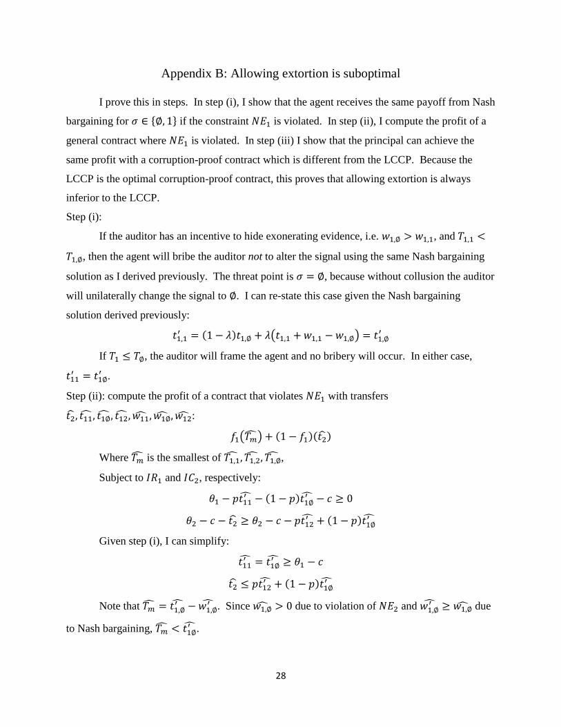
Appendix B: Allowing extortion is suboptimal

I prove this in steps. In step (i), I show that the agent receives the same payoff from Nash

bargaining for 𝜎 ∈ {∅, 1} if the constraint 𝑁𝐸1 is violated. In step (ii), I compute the profit of a

general contract where 𝑁𝐸1 is violated. In step (iii) I show that the principal can achieve the

same profit with a corruption-proof contract which is different from the LCCP. Because the

LCCP is the optimal corruption-proof contract, this proves that allowing extortion is always

inferior to the LCCP.

Step (i):

If the auditor has an incentive to hide exonerating evidence, i.e. 𝑤1,∅ > 𝑤1,1, and 𝑇1,1 <

𝑇1,∅, then the agent will bribe the auditor not to alter the signal using the same Nash bargaining

solution as I derived previously. The threat point is 𝜎 = ∅, because without collusion the auditor

will unilaterally change the signal to ∅. I can re-state this case given the Nash bargaining

solution derived previously:

𝑡1,1′ = (1 − 𝜆)𝑡1,∅ + 𝜆(𝑡1,1 + 𝑤1,1 − 𝑤1,∅) = 𝑡1,∅

′

If 𝑇1 ≤ 𝑇∅, the auditor will frame the agent and no bribery will occur. In either case,

𝑡11′ = 𝑡1∅

′ .

Step (ii): compute the profit of a contract that violates 𝑁𝐸1 with transfers

𝑡2̂, 𝑡11̂, 𝑡1∅̂, 𝑡12̂, 𝑤11̂, 𝑤1∅̂, 𝑤12̂:

𝑓1(𝑇�̂�) + (1 − 𝑓1)(𝑡2̂)

Where 𝑇�̂� is the smallest of 𝑇1,1̂, 𝑇1,2̂, 𝑇1,∅̂,

Subject to 𝐼𝑅1 and 𝐼𝐶2, respectively:

𝜃1 − 𝑝𝑡11′̂ − (1 − 𝑝)𝑡1∅

′̂ − 𝑐 ≥ 0

𝜃2 − 𝑐 − 𝑡2̂ ≥ 𝜃2 − 𝑐 − 𝑝𝑡12′̂ + (1 − 𝑝)𝑡1∅

′̂

Given step (i), I can simplify:

𝑡11′̂ = 𝑡1∅

′̂ ≥ 𝜃1 − 𝑐

𝑡2̂ ≤ 𝑝𝑡12′̂ + (1 − 𝑝)𝑡1∅

′̂

Note that 𝑇�̂� = 𝑡1,∅′̂ − 𝑤1,∅

′̂ . Since 𝑤1,∅̂ > 0 due to violation of 𝑁𝐸2 and 𝑤1,∅′̂ ≥ 𝑤1,∅̂ due

to Nash bargaining, 𝑇�̂� < 𝑡1∅′̂ .

29

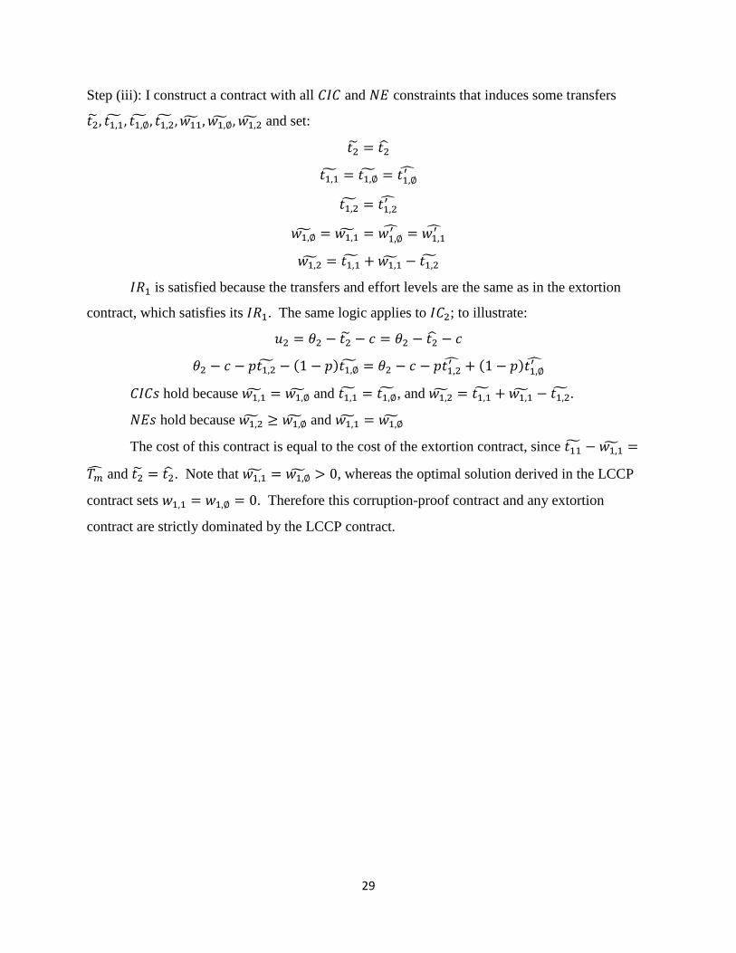
Step (iii): I construct a contract with all 𝐶𝐼𝐶 and 𝑁𝐸 constraints that induces some transfers

𝑡2̃, 𝑡1,1̃, 𝑡1,∅̃, 𝑡1,2̃, 𝑤11̃, 𝑤1,∅̃, 𝑤1,2̃ and set:

𝑡2̃ = 𝑡2̂

𝑡1,1̃ = 𝑡1,∅̃ = 𝑡1,∅′̂

𝑡1,2̃ = 𝑡1,2′̂

𝑤1,∅̃ = 𝑤1,1̃ = 𝑤1,∅′̂ = 𝑤1,1

′̂

𝑤1,2̃ = 𝑡1,1̃ + 𝑤1,1̃ − 𝑡1,2̃

𝐼𝑅1 is satisfied because the transfers and effort levels are the same as in the extortion

contract, which satisfies its 𝐼𝑅1. The same logic applies to 𝐼𝐶2; to illustrate:

𝑢2 = 𝜃2 − 𝑡2̃ − 𝑐 = 𝜃2 − 𝑡2̂ − 𝑐

𝜃2 − 𝑐 − 𝑝𝑡1,2̃ − (1 − 𝑝)𝑡1,∅̃ = 𝜃2 − 𝑐 − 𝑝𝑡1,2′̂ + (1 − 𝑝)𝑡1,∅

′̂

𝐶𝐼𝐶𝑠 hold because 𝑤1,1̃ = 𝑤1,∅̃ and 𝑡1,1̃ = 𝑡1,∅̃, and 𝑤1,2̃ = 𝑡1,1̃ + 𝑤1,1̃ − 𝑡1,2̃.

𝑁𝐸𝑠 hold because 𝑤1,2̃ ≥ 𝑤1,∅̃ and 𝑤1,1̃ = 𝑤1,∅̃

The cost of this contract is equal to the cost of the extortion contract, since 𝑡11̃ − 𝑤1,1̃ =

𝑇�̂� and 𝑡2̃ = 𝑡2̂. Note that 𝑤1,1̃ = 𝑤1,∅̃ > 0, whereas the optimal solution derived in the LCCP

contract sets 𝑤1,1 = 𝑤1,∅ = 0. Therefore this corruption-proof contract and any extortion

contract are strictly dominated by the LCCP contract.

30

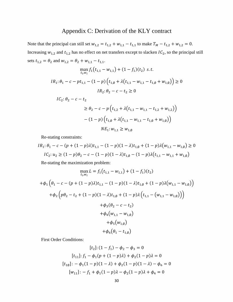
Appendix C: Derivation of the KLY contract

Note that the principal can still set 𝑤1,2 = 𝑡1,2 + 𝑤1,1 − 𝑡1,1 to make 𝑇𝑀 − 𝑡1,2 + 𝑤1,2 = 0.

Increasing 𝑤1,2 and 𝑡1,2 has no effect on net transfers except to slacken 𝐼𝐶2, so the principal still

sets 𝑡1,2 = 𝜃2 and 𝑤1,2 = 𝜃2 + 𝑤1,1 − 𝑡1,1.

max𝑡𝑖,𝑤𝑖

𝑓1(𝑡1,1 − 𝑤1,1) + (1 − 𝑓1)(𝑡2) 𝑠. 𝑡.

𝐼𝑅1: 𝜃1 − 𝑐 − 𝑝𝑡1,1 − (1 − 𝑝) (𝑡1,∅ + 𝜆(𝑡1,1 − 𝑤1,1 − 𝑡1,∅ + 𝑤1,∅)) ≥ 0

𝐼𝑅2: 𝜃2 − 𝑐 − 𝑡2 ≥ 0

𝐼𝐶2: 𝜃2 − 𝑐 − 𝑡2

≥ 𝜃2 − 𝑐 − 𝑝 (𝑡1,2 + 𝜆(𝑡1,1 − 𝑤1,1 − 𝑡1,2 + 𝑤1,2))

− (1 − 𝑝) (𝑡1,∅ + 𝜆(𝑡1,1 − 𝑤1,1 − 𝑡1,∅ + 𝑤1,∅))

𝑁𝐸1: 𝑤1,1 ≥ 𝑤1,∅

Re-stating constraints:

𝐼𝑅1: 𝜃1 − 𝑐 − (𝑝 + (1 − 𝑝)𝜆)𝑡1,1 − (1 − 𝑝)(1 − 𝜆)𝑡1,∅ + (1 − 𝑝)𝜆(𝑤1,1 − 𝑤1,∅) ≥ 0

𝐼𝐶2: 𝑢2 ≥ (1 − 𝑝)𝜃2 − 𝑐 − (1 − 𝑝)(1 − 𝜆)𝑡1,∅ − (1 − 𝑝)𝜆(𝑡1,1 − 𝑤1,1 + 𝑤1,∅)

Re-stating the maximization problem:

max𝑡𝑖,𝑤𝑖

𝐿 = 𝑓1(𝑡1,1 − 𝑤1,1) + (1 − 𝑓1)(𝑡2)

+𝜙1 (𝜃1 − 𝑐 − (𝑝 + (1 − 𝑝)𝜆)𝑡1,1 − (1 − 𝑝)(1 − 𝜆)𝑡1,∅ + (1 − 𝑝)𝜆(𝑤1,1 − 𝑤1,∅))

+𝜙2 (𝑝𝜃2 − 𝑡2 + (1 − 𝑝)(1 − 𝜆)𝑡1,∅ + (1 − 𝑝)𝜆 (𝑡1,1 − (𝑤1,1 − 𝑤1,∅)))

+𝜙3(𝜃2 − 𝑐 − 𝑡2)

+𝜙4(𝑤1,1 − 𝑤1,∅)

+𝜙5(𝑤1,∅)

+𝜙6(𝜃1 − 𝑡1,∅)

First Order Conditions:

[𝑡2]: (1 − 𝑓1) − 𝜙2 − 𝜙3 = 0

[𝑡11]: 𝑓1 − 𝜙1(𝑝 + (1 − 𝑝)𝜆) + 𝜙2(1 − 𝑝)𝜆 = 0

[𝑡1∅] : − 𝜙1(1 − 𝑝)(1 − 𝜆) + 𝜙2(1 − 𝑝)(1 − 𝜆) − 𝜙6 = 0

[𝑤11] : − 𝑓1 + 𝜙1(1 − 𝑝)𝜆 − 𝜙2(1 − 𝑝)𝜆 + 𝜙4 = 0

31

[𝑤1∅] : − 𝜙1(1 − 𝑝)𝜆 + 𝜙2(1 − 𝑝)𝜆 − 𝜙4 + 𝜙5 = 0

Solving:

𝜙5 = 𝑓1; 𝑤1,∅ = 0

𝜙1(1 − 𝑝)𝜆 − 𝜙2(1 − 𝑝)𝜆 + 𝜙4 = 𝑓1

𝜙1(𝑝 + (1 − 𝑝)𝜆) − 𝜙2(1 − 𝑝)𝜆 = 𝑓1

𝜙4 = 𝜙1𝑝; 𝑤1,1 = 0

𝜙1 =𝑓1 + 𝜙2(1 − 𝑝)𝜆

𝑝 + (1 − 𝑝)𝜆

𝜙6 = 𝜙2(1 − 𝑝)(1 − 𝜆) −𝑓1 + 𝜙2(1 − 𝑝)𝜆

𝑝 + (1 − 𝑝)𝜆(1 − 𝑝)(1 − 𝜆)

𝜙6

𝑝 + (1 − 𝑝)𝜆

(1 − 𝑝)(1 − 𝜆)= 𝜙2(𝑝 + (1 − 𝑝)𝜆) − 𝑓1 − 𝜙2(1 − 𝑝)𝜆

𝜙6

𝑝 + (1 − 𝑝)𝜆

(1 − 𝑝)(1 − 𝜆)= 𝜙2𝑝 − 𝑓1

𝜙2 = 1 − 𝑓1 − 𝜙3

(1 − 𝑓1 − 𝜙3)𝑝 − 𝑓1 = 𝜙6

𝑝 + (1 − 𝑝)𝜆

(1 − 𝑝)(1 − 𝜆)

𝑝 =𝑓1

1 − 𝑓1 − 𝜙3+ 𝜙6

𝑝 + (1 − 𝑝)𝜆

(1 − 𝑝)(1 − 𝜆)

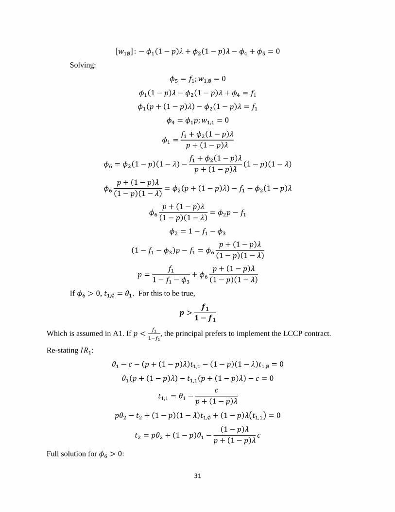
If 𝜙6 > 0, 𝑡1,∅ = 𝜃1. For this to be true,

𝒑 >𝒇𝟏

𝟏 − 𝒇𝟏

Which is assumed in A1. If 𝑝 <𝑓1

1−𝑓1, the principal prefers to implement the LCCP contract.

Re-stating 𝐼𝑅1:

𝜃1 − 𝑐 − (𝑝 + (1 − 𝑝)𝜆)𝑡1,1 − (1 − 𝑝)(1 − 𝜆)𝑡1,∅ = 0

𝜃1(𝑝 + (1 − 𝑝)𝜆) − 𝑡1,1(𝑝 + (1 − 𝑝)𝜆) − 𝑐 = 0

𝑡1,1 = 𝜃1 −𝑐

𝑝 + (1 − 𝑝)𝜆

𝑝𝜃2 − 𝑡2 + (1 − 𝑝)(1 − 𝜆)𝑡1,∅ + (1 − 𝑝)𝜆(𝑡1,1) = 0

𝑡2 = 𝑝𝜃2 + (1 − 𝑝)𝜃1 −(1 − 𝑝)𝜆

𝑝 + (1 − 𝑝)𝜆𝑐

Full solution for 𝜙6 > 0:

32

𝑤1,1 = 𝑤1,∅ = 0

𝑡1,2 = 𝜃2

𝑤1,2 = 𝜃2 − 𝜃1 +𝑐

𝑝 + (1 − 𝑝)𝜆

𝑡1,1 = 𝜃1 −𝑐

𝑝 + (1 − 𝑝)𝜆

𝑡1,∅ = 𝜃1

𝑡2 = 𝑝𝜃2 + (1 − 𝑝)𝜃1 −(1 − 𝑝)𝜆

𝑝 + (1 − 𝑝)𝜆𝑐

𝑢2 = (1 − 𝑝)Δ𝜃 −𝑝

𝑝 + (1 − 𝑝)𝜆𝑐

This is the solution so long as

(1 − 𝑝)Δ𝜃 ≥𝑝

𝑝 + (1 − 𝑝)𝜆𝑐

Which is true as long as A2 holds.

If 𝜙3 > 0, 𝜙6 = 0, 𝑡1,∅ < 𝜃1. In this case 𝑡1,∅ is determined by the minimum amount it

can be while still having a binding 𝐼𝑅2. Solving:

𝒖𝟐 = 𝟎; 𝒕𝟐 = 𝜽𝟐 − 𝒄

(1 − 𝑝)𝜃2 − 𝑐 − (1 − 𝑝)(1 − 𝜆)𝑡1,∅ − (1 − 𝑝)𝜆𝑡1,1 = 0

𝜃1 − 𝑐 − (𝑝 + (1 − 𝑝)𝜆)𝑡1,1 − (1 − 𝑝)(1 − 𝜆)𝑡1,∅ = 0

𝑡1,1 =𝜃1 − 𝑐 − (1 − 𝑝)(1 − 𝜆)𝑡1,∅

𝑝 + (1 − 𝑝)𝜆

(1 − 𝑝)𝜃2 − 𝑐 − (1 − 𝑝)(1 − 𝜆)𝑡1,∅ − (1 − 𝑝)𝜆𝜃1 − 𝑐 − (1 − 𝑝)(1 − 𝜆)𝑡1,∅

𝑝 + (1 − 𝑝)𝜆= 0

(1 − 𝑝)𝜃2 − 𝑐 (1 −(1 − 𝑝)𝜆

𝑝 + (1 − 𝑝)𝜆) − 𝑡1,∅(1 − 𝑝)(1 − 𝜆) (1 −

(1 − 𝑝)𝜆

𝑝 + (1 − 𝑝)𝜆)

(1 − 𝑝)𝜃2 −(1 − 𝑝)𝜆

𝑝 + (1 − 𝑝)𝜆𝜃1 −

𝑝

𝑝 + (1 − 𝑝)𝜆𝑐 − (1 − 𝑝)(1 − 𝜆)

𝑝

𝑝 + (1 − 𝑝)𝜆𝑡1,∅ = 0

(1 − 𝑝)(1 − 𝜆)𝑝

𝑝 + (1 − 𝑝)𝜆𝑡1,∅ = (1 − 𝑝)𝜃2 −

(1 − 𝑝)𝜆

𝑝 + (1 − 𝑝)𝜆𝜃1 −

𝑝

𝑝 + (1 − 𝑝)𝜆𝑐

𝑡1,∅ =(1 − 𝑝)(𝑝 + (1 − 𝑝)𝜆)

(1 − 𝑝)(1 − 𝜆)𝑝𝜃2 −

(1 − 𝑝)𝜆

(1 − 𝑝)(1 − 𝜆)𝑝𝜃1 −

𝑝

(1 − 𝑝)(1 − 𝜆)𝑝𝑐

𝑡1,∅ =𝑝 + (1 − 𝑝)𝜆

𝑝(1 − 𝜆)𝜃2 −

𝜆

𝑝(1 − 𝜆)𝜃1 −

𝑐

(1 − 𝑝)(1 − 𝜆)

33

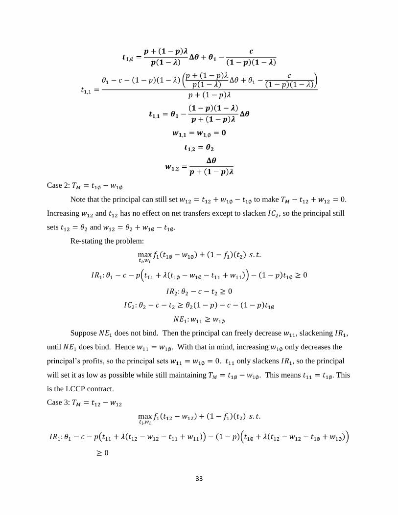
𝒕𝟏,∅ =𝒑 + (𝟏 − 𝒑)𝝀

𝒑(𝟏 − 𝝀)𝚫𝜽 + 𝜽𝟏 −

𝒄

(𝟏 − 𝒑)(𝟏 − 𝝀)

𝑡1,1 =𝜃1 − 𝑐 − (1 − 𝑝)(1 − 𝜆) (

𝑝 + (1 − 𝑝)𝜆𝑝(1 − 𝜆)

Δ𝜃 + 𝜃1 −𝑐

(1 − 𝑝)(1 − 𝜆))

𝑝 + (1 − 𝑝)𝜆

𝒕𝟏,𝟏 = 𝜽𝟏 −(𝟏 − 𝒑)(𝟏 − 𝝀)

𝒑 + (𝟏 − 𝒑)𝝀𝚫𝜽

𝒘𝟏,𝟏 = 𝒘𝟏,∅ = 𝟎

𝒕𝟏,𝟐 = 𝜽𝟐

𝒘𝟏,𝟐 =𝚫𝜽

𝒑 + (𝟏 − 𝒑)𝝀

Case 2: 𝑇𝑀 = 𝑡1∅ − 𝑤1∅

Note that the principal can still set 𝑤12 = 𝑡12 + 𝑤1∅ − 𝑡1∅ to make 𝑇𝑀 − 𝑡12 + 𝑤12 = 0.

Increasing 𝑤12 and 𝑡12 has no effect on net transfers except to slacken 𝐼𝐶2, so the principal still

sets 𝑡12 = 𝜃2 and 𝑤12 = 𝜃2 + 𝑤1∅ − 𝑡1∅.

Re-stating the problem:

max𝑡𝑖,𝑤𝑖

𝑓1(𝑡1∅ − 𝑤1∅) + (1 − 𝑓1)(𝑡2) 𝑠. 𝑡.

𝐼𝑅1: 𝜃1 − 𝑐 − 𝑝(𝑡11 + 𝜆(𝑡1∅ − 𝑤1∅ − 𝑡11 + 𝑤11)) − (1 − 𝑝)𝑡1∅ ≥ 0

𝐼𝑅2: 𝜃2 − 𝑐 − 𝑡2 ≥ 0

𝐼𝐶2: 𝜃2 − 𝑐 − 𝑡2 ≥ 𝜃2(1 − 𝑝) − 𝑐 − (1 − 𝑝)𝑡1∅

𝑁𝐸1: 𝑤11 ≥ 𝑤1∅

Suppose 𝑁𝐸1 does not bind. Then the principal can freely decrease 𝑤11, slackening 𝐼𝑅1,

until 𝑁𝐸1 does bind. Hence 𝑤11 = 𝑤1∅. With that in mind, increasing 𝑤1∅ only decreases the

principal’s profits, so the principal sets 𝑤11 = 𝑤1∅ = 0. 𝑡11 only slackens 𝐼𝑅1, so the principal

will set it as low as possible while still maintaining 𝑇𝑀 = 𝑡1∅ − 𝑤1∅. This means 𝑡11 = 𝑡1∅. This

is the LCCP contract.

Case 3: 𝑇𝑀 = 𝑡12 − 𝑤12

max𝑡𝑖,𝑤𝑖

𝑓1(𝑡12 − 𝑤12) + (1 − 𝑓1)(𝑡2) 𝑠. 𝑡.

𝐼𝑅1: 𝜃1 − 𝑐 − 𝑝(𝑡11 + 𝜆(𝑡12 − 𝑤12 − 𝑡11 + 𝑤11)) − (1 − 𝑝)(𝑡1∅ + 𝜆(𝑡12 − 𝑤12 − 𝑡1∅ + 𝑤1∅))

≥ 0

34

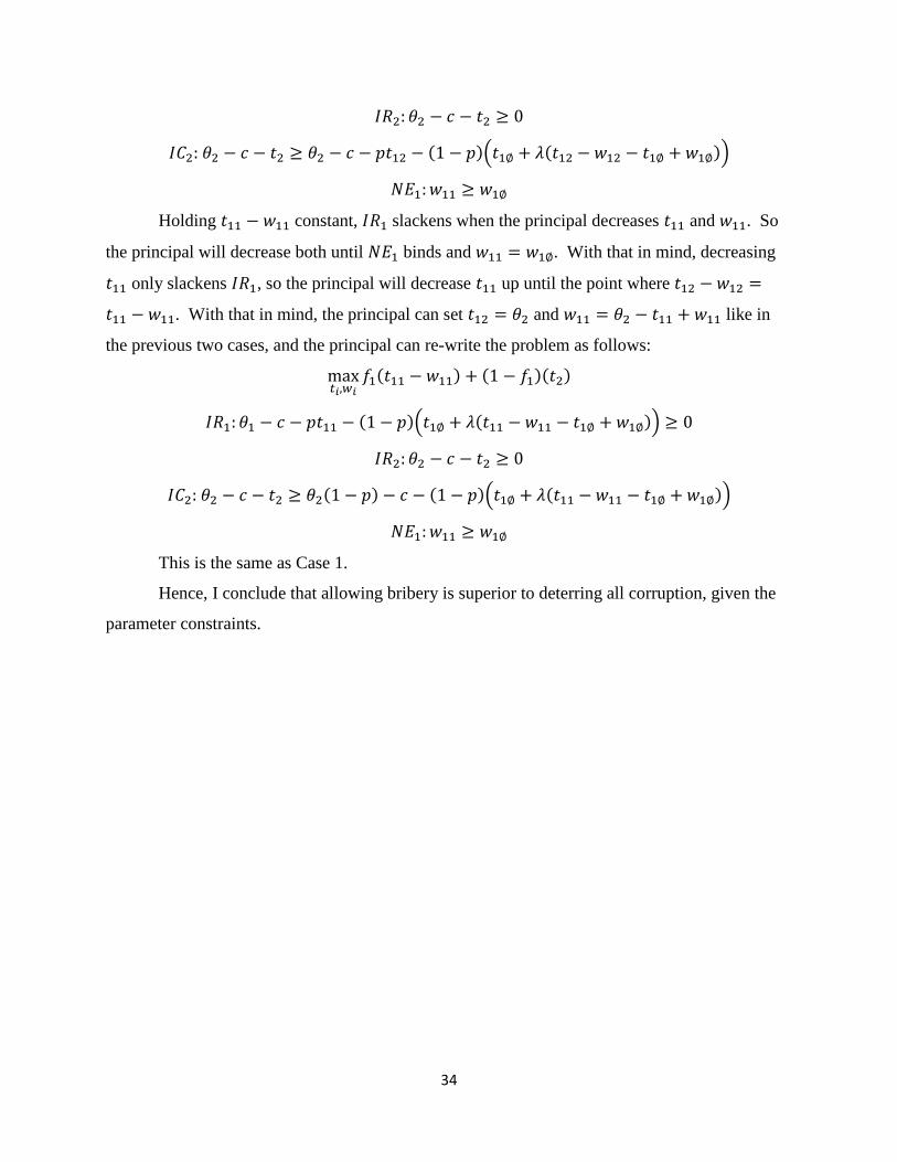
𝐼𝑅2: 𝜃2 − 𝑐 − 𝑡2 ≥ 0

𝐼𝐶2: 𝜃2 − 𝑐 − 𝑡2 ≥ 𝜃2 − 𝑐 − 𝑝𝑡12 − (1 − 𝑝)(𝑡1∅ + 𝜆(𝑡12 − 𝑤12 − 𝑡1∅ + 𝑤1∅))

𝑁𝐸1: 𝑤11 ≥ 𝑤1∅

Holding 𝑡11 − 𝑤11 constant, 𝐼𝑅1 slackens when the principal decreases 𝑡11 and 𝑤11. So

the principal will decrease both until 𝑁𝐸1 binds and 𝑤11 = 𝑤1∅. With that in mind, decreasing

𝑡11 only slackens 𝐼𝑅1, so the principal will decrease 𝑡11 up until the point where 𝑡12 − 𝑤12 =

𝑡11 − 𝑤11. With that in mind, the principal can set 𝑡12 = 𝜃2 and 𝑤11 = 𝜃2 − 𝑡11 + 𝑤11 like in

the previous two cases, and the principal can re-write the problem as follows:

max𝑡𝑖,𝑤𝑖

𝑓1(𝑡11 − 𝑤11) + (1 − 𝑓1)(𝑡2)

𝐼𝑅1: 𝜃1 − 𝑐 − 𝑝𝑡11 − (1 − 𝑝)(𝑡1∅ + 𝜆(𝑡11 − 𝑤11 − 𝑡1∅ + 𝑤1∅)) ≥ 0

𝐼𝑅2: 𝜃2 − 𝑐 − 𝑡2 ≥ 0

𝐼𝐶2: 𝜃2 − 𝑐 − 𝑡2 ≥ 𝜃2(1 − 𝑝) − 𝑐 − (1 − 𝑝)(𝑡1∅ + 𝜆(𝑡11 − 𝑤11 − 𝑡1∅ + 𝑤1∅))

𝑁𝐸1: 𝑤11 ≥ 𝑤1∅

This is the same as Case 1.

Hence, I conclude that allowing bribery is superior to deterring all corruption, given the

parameter constraints.

35

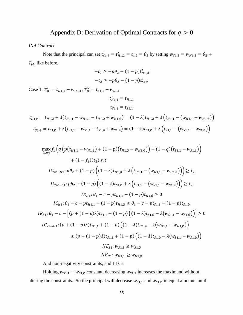
Appendix D: Derivation of Optimal Contracts for 𝑞 > 0

INA Contract

Note that the principal can set 𝑡𝑆1,2′ = 𝑡𝐻1,2

′ = 𝑡1,2 = 𝜃2 by setting 𝑤𝑆1,2 = 𝑤𝐻1,2 = 𝜃2 +

𝑇𝑀, like before.

−𝑡2 ≥ −𝑝𝜃2 − (1 − 𝑝)𝑡𝐻1,∅′

−𝑡2 ≥ −𝑝𝜃2 − (1 − 𝑝)𝑡𝑆1,∅′

Case 1: 𝑇𝑀𝐻 = 𝑡𝐻1,1 − 𝑤𝐻1,1, 𝑇𝑀

𝑆 = 𝑡𝑆1,1 − 𝑤𝑆1,1

𝑡𝐻1,1′ = 𝑡𝐻1,1

𝑡𝑆1,1′ = 𝑡𝑆1,1

𝑡𝐻1,∅′ = 𝑡𝐻1,∅ + 𝜆(𝑡𝐻1,1 − 𝑤𝐻1,1 − 𝑡𝐻1,∅ + 𝑤𝐻1,∅) = (1 − 𝜆)𝑡𝐻1,∅ + 𝜆 (𝑡𝐻1,1 − (𝑤𝐻1,1 − 𝑤𝐻1,∅))

𝑡𝑆1,∅′ = 𝑡𝑆1,∅ + 𝜆(𝑡𝑆1,1 − 𝑤𝑆1,1 − 𝑡𝑆1,∅ + 𝑤𝑆1,∅) = (1 − 𝜆)𝑡𝑆1,∅ + 𝜆 (𝑡𝑆1,1 − (𝑤𝑆1,1 − 𝑤𝑆1,∅))

max𝑡𝑖,𝑤𝑖

𝑓1 (𝑞 (𝑝(𝑡𝐻1,1 − 𝑤𝐻1,1) + (1 − 𝑝)(𝑡𝐻1,∅ − 𝑤𝐻1,∅)) + (1 − 𝑞)(𝑡𝑆1,1 − 𝑤𝑆1,1))

+ (1 − 𝑓1)(𝑡2) 𝑠. 𝑡.

𝐼𝐶𝑆2→𝐻1: 𝑝𝜃2 + (1 − 𝑝) ((1 − 𝜆)𝑡𝐻1,∅ + 𝜆 (𝑡𝐻1,1 − (𝑤𝐻1,1 − 𝑤𝐻1,∅))) ≥ 𝑡2

𝐼𝐶𝑆2→𝑆1: 𝑝𝜃2 + (1 − 𝑝) ((1 − 𝜆)𝑡𝑆1,∅ + 𝜆 (𝑡𝑆1,1 − (𝑤𝑆1,1 − 𝑤𝑆1,∅))) ≥ 𝑡2

𝐼𝑅𝐻1: 𝜃1 − 𝑐 − 𝑝𝑡𝐻1,1 − (1 − 𝑝)𝑡𝐻1,∅ ≥ 0

𝐼𝐶𝐻1: 𝜃1 − 𝑐 − 𝑝𝑡𝐻1,1 − (1 − 𝑝)𝑡𝐻1,∅ ≥ 𝜃1 − 𝑐 − 𝑝𝑡𝑆1,1 − (1 − 𝑝)𝑡𝑆1,∅

𝐼𝑅𝑆1: 𝜃1 − 𝑐 − [(𝑝 + (1 − 𝑝)𝜆)𝑡𝑆1,1 + (1 − 𝑝) ((1 − 𝜆)𝑡𝑆1,∅ − 𝜆(𝑤𝑆1,1 − 𝑤𝑆1,∅))] ≥ 0

𝐼𝐶𝑆1→𝐻1: (𝑝 + (1 − 𝑝)𝜆)𝑡𝐻1,1 + (1 − 𝑝) ((1 − 𝜆)𝑡𝐻1,∅ − 𝜆(𝑤𝐻1,1 − 𝑤𝐻1,∅))

≥ (𝑝 + (1 − 𝑝)𝜆)𝑡𝑆1,1 + (1 − 𝑝) ((1 − 𝜆)𝑡𝑆1,∅ − 𝜆(𝑤𝑆1,1 − 𝑤𝑆1,∅))

𝑁𝐸𝑆1: 𝑤𝑆1,1 ≥ 𝑤𝑆1,∅

𝑁𝐸𝐻1: 𝑤𝐻1,1 ≥ 𝑤𝐻1,∅

And non-negativity constraints, and LLCs.

Holding 𝑤𝑆1,1 − 𝑤𝑆1,∅ constant, decreasing 𝑤𝑆1,1 increases the maximand without

altering the constraints. So the principal will decrease 𝑤𝑆1,1 and 𝑤𝑆1,∅ in equal amounts until

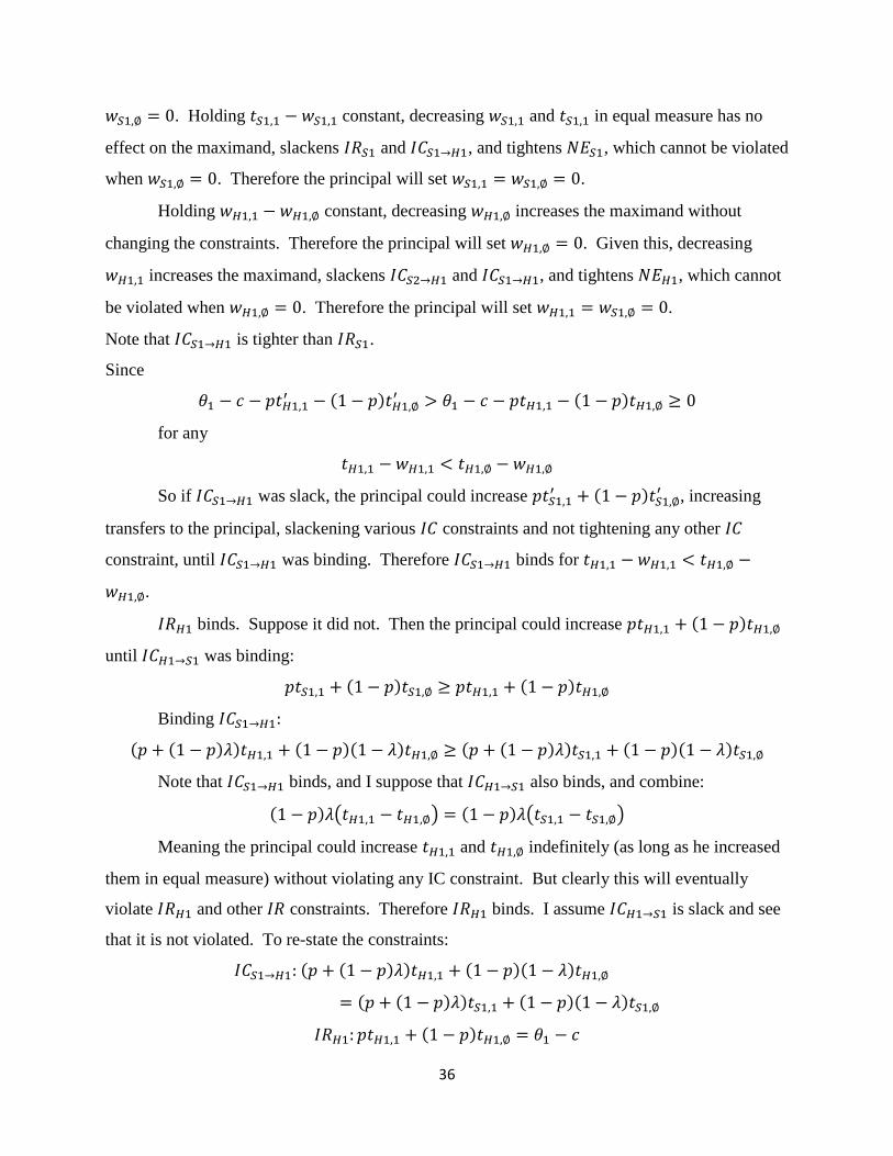
36

𝑤𝑆1,∅ = 0. Holding 𝑡𝑆1,1 − 𝑤𝑆1,1 constant, decreasing 𝑤𝑆1,1 and 𝑡𝑆1,1 in equal measure has no

effect on the maximand, slackens 𝐼𝑅𝑆1 and 𝐼𝐶𝑆1→𝐻1, and tightens 𝑁𝐸𝑆1, which cannot be violated

when 𝑤𝑆1,∅ = 0. Therefore the principal will set 𝑤𝑆1,1 = 𝑤𝑆1,∅ = 0.

Holding 𝑤𝐻1,1 − 𝑤𝐻1,∅ constant, decreasing 𝑤𝐻1,∅ increases the maximand without

changing the constraints. Therefore the principal will set 𝑤𝐻1,∅ = 0. Given this, decreasing

𝑤𝐻1,1 increases the maximand, slackens 𝐼𝐶𝑆2→𝐻1 and 𝐼𝐶𝑆1→𝐻1, and tightens 𝑁𝐸𝐻1, which cannot

be violated when 𝑤𝐻1,∅ = 0. Therefore the principal will set 𝑤𝐻1,1 = 𝑤𝑆1,∅ = 0.

Note that 𝐼𝐶𝑆1→𝐻1 is tighter than 𝐼𝑅𝑆1.

Since

𝜃1 − 𝑐 − 𝑝𝑡𝐻1,1′ − (1 − 𝑝)𝑡𝐻1,∅

′ > 𝜃1 − 𝑐 − 𝑝𝑡𝐻1,1 − (1 − 𝑝)𝑡𝐻1,∅ ≥ 0

for any

𝑡𝐻1,1 − 𝑤𝐻1,1 < 𝑡𝐻1,∅ − 𝑤𝐻1,∅

So if 𝐼𝐶𝑆1→𝐻1 was slack, the principal could increase 𝑝𝑡𝑆1,1′ + (1 − 𝑝)𝑡𝑆1,∅

′ , increasing

transfers to the principal, slackening various 𝐼𝐶 constraints and not tightening any other 𝐼𝐶

constraint, until 𝐼𝐶𝑆1→𝐻1 was binding. Therefore 𝐼𝐶𝑆1→𝐻1 binds for 𝑡𝐻1,1 − 𝑤𝐻1,1 < 𝑡𝐻1,∅ −

𝑤𝐻1,∅.

𝐼𝑅𝐻1 binds. Suppose it did not. Then the principal could increase 𝑝𝑡𝐻1,1 + (1 − 𝑝)𝑡𝐻1,∅

until 𝐼𝐶𝐻1→𝑆1 was binding:

𝑝𝑡𝑆1,1 + (1 − 𝑝)𝑡𝑆1,∅ ≥ 𝑝𝑡𝐻1,1 + (1 − 𝑝)𝑡𝐻1,∅

Binding 𝐼𝐶𝑆1→𝐻1:

(𝑝 + (1 − 𝑝)𝜆)𝑡𝐻1,1 + (1 − 𝑝)(1 − 𝜆)𝑡𝐻1,∅ ≥ (𝑝 + (1 − 𝑝)𝜆)𝑡𝑆1,1 + (1 − 𝑝)(1 − 𝜆)𝑡𝑆1,∅

Note that 𝐼𝐶𝑆1→𝐻1 binds, and I suppose that 𝐼𝐶𝐻1→𝑆1 also binds, and combine:

(1 − 𝑝)𝜆(𝑡𝐻1,1 − 𝑡𝐻1,∅) = (1 − 𝑝)𝜆(𝑡𝑆1,1 − 𝑡𝑆1,∅)

Meaning the principal could increase 𝑡𝐻1,1 and 𝑡𝐻1,∅ indefinitely (as long as he increased

them in equal measure) without violating any IC constraint. But clearly this will eventually

violate 𝐼𝑅𝐻1 and other 𝐼𝑅 constraints. Therefore 𝐼𝑅𝐻1 binds. I assume 𝐼𝐶𝐻1→𝑆1 is slack and see

that it is not violated. To re-state the constraints:

𝐼𝐶𝑆1→𝐻1: (𝑝 + (1 − 𝑝)𝜆)𝑡𝐻1,1 + (1 − 𝑝)(1 − 𝜆)𝑡𝐻1,∅

= (𝑝 + (1 − 𝑝)𝜆)𝑡𝑆1,1 + (1 − 𝑝)(1 − 𝜆)𝑡𝑆1,∅

𝐼𝑅𝐻1: 𝑝𝑡𝐻1,1 + (1 − 𝑝)𝑡𝐻1,∅ = 𝜃1 − 𝑐

37

𝐼𝐶𝑆2→𝐻1: 𝑝𝜃2 + (1 − 𝑝) ((1 − 𝜆)𝑡𝐻1,∅ + 𝜆𝑡𝐻1,1) ≥ 𝑡2

𝐼𝐶𝑆2−𝑆1: 𝑝𝜃2 + (1 − 𝑝) ((1 − 𝜆)𝑡𝑆1,∅ + 𝜆𝑡𝑆1,1) ≥ 𝑡2

Suppose 𝐼𝐶𝑆2→𝑆1 does not bind. Given that 𝐼𝐶𝑆1→𝐻1 binds the principal can maintain

𝑆1’s rent but decrease the net transfer to the auditor-agent coalition (by reducing the bribe paid

to the auditor) by increasing 𝑡11𝑆 and decreasing 𝑡1∅

𝑆 . Therefore 𝐼𝐶𝑆2→𝑆1 binds. Re-writing S1’s

rent given binding 𝐼𝑅𝐻1 and 𝐼𝐶𝑆1→𝐻1:

𝑡𝐻1,1 =𝜃1 − 𝑐 − (1 − 𝑝)𝑡𝐻1,∅

𝑝

(𝑝 + (1 − 𝑝)𝜆)𝑡𝑆1,1 + (1 − 𝑝)(1 − 𝜆)𝑡𝑆1,∅ = (𝑝 + (1 − 𝑝)𝜆)𝑡𝐻1,1 + (1 − 𝑝)(1 − 𝜆)𝑡𝐻1,∅

(𝑝 + (1 − 𝑝)𝜆)𝑡𝑆1,1 + (1 − 𝑝)(1 − 𝜆)𝑡𝑆1,∅ =𝑝 + (1 − 𝑝)𝜆

𝑝(𝜃1 − 𝑐) −

(1 − 𝑝)𝜆

𝑝𝑡𝐻1,∅

Suppose 𝐼𝐶𝑆2→𝐻1 does not bind. Then the principal could increase 𝑡1∅𝐻 and decrease 𝑡11

𝐻

to decrease 𝑆1’s rent until 𝐼𝐶𝑆2→𝐻1 became binding. Therefore 𝐼𝐶𝑆2→𝐻1 binds. Combining

𝐼𝐶𝑆2→𝐻1 and 𝐼𝐶𝑆2→𝑆1:

(1 − 𝜆)𝑡𝐻1,∅ + 𝜆𝑡𝐻1,1 = (1 − 𝜆)𝑡𝑆1,∅ + 𝜆𝑡𝑆1,1

Multiply by (1 − 𝑝)

(1 − 𝑝)(1 − 𝜆)𝑡𝐻1,∅ + (1 − 𝑝)𝜆𝑡𝐻1,1 = (1 − 𝑝)(1 − 𝜆)𝑡𝑆1,∅ + (1 − 𝑝)𝜆𝑡𝑆1,1

Combine with 𝐼𝐶𝑆1→𝐻1

𝑝𝑡𝐻1,1 = 𝑝𝑡𝑆1,1

𝑡𝐻1,1 = 𝑡𝑆1,1 = 𝑡1,1

𝑡𝐻1,∅ = 𝑡𝑆1,∅ = 𝑡1,∅

Given this knowledge I can solve the problem as follows:

max𝑡𝑖,𝑤𝑖

𝐿 = 𝑓1(𝑞(𝑝𝑡1,1 + (1 − 𝑝)𝑡1,∅) + (1 − 𝑞)𝑡1,1) + (1 − 𝑓1)(𝑡2)

+𝜙1(𝜃1 − 𝑐 − 𝑝𝑡1,1 − (1 − 𝑝)𝑡1,∅)

+𝜙2 (𝑝𝜃2 + (1 − 𝑝) ((1 − 𝜆)𝑡1,∅ + 𝜆𝑡1,1) − 𝑡2)

+𝜙3(𝜃1 − 𝑡1,∅)

First order conditions:

[𝑡11]: 𝑓1(𝑞𝑝 + (1 − 𝑞)) − 𝜙1𝑝 + 𝜙2(1 − 𝑝)𝜆 = 0

[𝑡1∅]: 𝑓1𝑞(1 − 𝑝) − 𝜙1(1 − 𝑝) + 𝜙2(1 − 𝑝)(1 − 𝜆) − 𝜙3 = 0

38

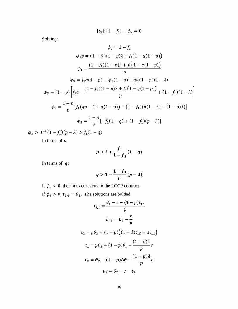
[𝑡2]: (1 − 𝑓1) − 𝜙2 = 0

Solving:

𝜙2 = 1 − 𝑓1

𝜙1𝑝 = (1 − 𝑓1)(1 − 𝑝)𝜆 + 𝑓1(1 − 𝑞(1 − 𝑝))

𝜙1 =(1 − 𝑓1)(1 − 𝑝)𝜆 + 𝑓1(1 − 𝑞(1 − 𝑝))

𝑝

𝜙3 = 𝑓1𝑞(1 − 𝑝) − 𝜙1(1 − 𝑝) + 𝜙2(1 − 𝑝)(1 − 𝜆)

𝜙3 = (1 − 𝑝) [𝑓1𝑞 −(1 − 𝑓1)(1 − 𝑝)𝜆 + 𝑓1(1 − 𝑞(1 − 𝑝))

𝑝+ (1 − 𝑓1)(1 − 𝜆)]

𝜙3 =1 − 𝑝

𝑝[𝑓1(𝑞𝑝 − 1 + 𝑞(1 − 𝑝)) + (1 − 𝑓1)(𝑝(1 − 𝜆) − (1 − 𝑝)𝜆)]

𝜙3 =1 − 𝑝

𝑝[−𝑓1(1 − 𝑞) + (1 − 𝑓1)(𝑝 − 𝜆)]

𝜙3 > 0 if (1 − 𝑓1)(𝑝 − 𝜆) > 𝑓1(1 − 𝑞)

In terms of 𝑝:

𝒑 > 𝝀 +𝒇𝟏

𝟏 − 𝒇𝟏

(𝟏 − 𝒒)

In terms of 𝑞:

𝒒 > 𝟏 −𝟏 − 𝒇𝟏

𝒇𝟏

(𝒑 − 𝝀)

If 𝜙3 < 0, the contract reverts to the LCCP contract.

If 𝜙3 > 0, 𝒕𝟏,∅ = 𝜽𝟏. The solutions are bolded:

𝑡1,1 =𝜃1 − 𝑐 − (1 − 𝑝)𝑡1∅

𝑝

𝒕𝟏,𝟏 = 𝜽𝟏 −𝒄

𝒑

𝑡2 = 𝑝𝜃2 + (1 − 𝑝)((1 − 𝜆)𝑡1∅ + 𝜆𝑡11)

𝑡2 = 𝑝𝜃2 + (1 − 𝑝)𝜃1 −(1 − 𝑝)𝜆

𝑝𝑐

𝒕𝟐 = 𝜽𝟐 − (𝟏 − 𝒑)𝚫𝜽 −(𝟏 − 𝒑)𝝀

𝒑𝒄

𝑢2 = 𝜃2 − 𝑐 − 𝑡2

39

𝑢2 = 𝜃2 − 𝑐 − 𝜃2 + (1 − 𝑝)Δ𝜃 +(1 − 𝑝)𝜆

𝑝𝑐

𝑢2 = (1 − 𝑝)Δ𝜃 −𝑝 − (1 − 𝑝)𝜆

𝑝𝑐

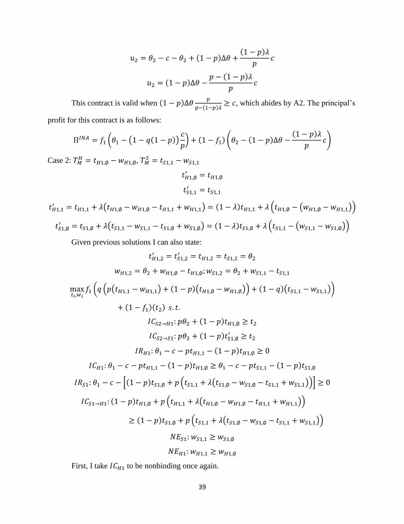
This contract is valid when (1 − 𝑝)Δ𝜃𝑝

𝑝−(1−𝑝)𝜆≥ 𝑐, which abides by A2. The principal’s

profit for this contract is as follows:

Π𝐼𝑁𝐴 = 𝑓1 (𝜃1 − (1 − 𝑞(1 − 𝑝))𝑐

𝑝) + (1 − 𝑓1) (𝜃2 − (1 − 𝑝)Δ𝜃 −

(1 − 𝑝)𝜆

𝑝𝑐)

Case 2: 𝑇𝑀𝐻 = 𝑡𝐻1,∅ − 𝑤𝐻1,∅, 𝑇𝑀

𝑆 = 𝑡𝑆1,1 − 𝑤𝑆1,1

𝑡𝐻1,∅′ = 𝑡𝐻1,∅

𝑡𝑆1,1′ = 𝑡𝑆1,1

𝑡𝐻1,1′ = 𝑡𝐻1,1 + 𝜆(𝑡𝐻1,∅ − 𝑤𝐻1,∅ − 𝑡𝐻1,1 + 𝑤𝐻1,1) = (1 − 𝜆)𝑡𝐻1,1 + 𝜆 (𝑡𝐻1,∅ − (𝑤𝐻1,∅ − 𝑤𝐻1,1))

𝑡𝑆1,∅′ = 𝑡𝑆1,∅ + 𝜆(𝑡𝑆1,1 − 𝑤𝑆1,1 − 𝑡𝑆1,∅ + 𝑤𝑆1,∅) = (1 − 𝜆)𝑡𝑆1,∅ + 𝜆 (𝑡𝑆1,1 − (𝑤𝑆1,1 − 𝑤𝑆1,∅))

Given previous solutions I can also state:

𝑡𝐻1,2′ = 𝑡𝑆1,2

′ = 𝑡𝐻1,2 = 𝑡𝑆1,2 = 𝜃2

𝑤𝐻1,2 = 𝜃2 + 𝑤𝐻1,∅ − 𝑡𝐻1,∅; 𝑤𝑆1,2 = 𝜃2 + 𝑤𝑆1,1 − 𝑡𝑆1,1

max𝑡𝑖,𝑤𝑖

𝑓1 (𝑞 (𝑝(𝑡𝐻1,1 − 𝑤𝐻1,1) + (1 − 𝑝)(𝑡𝐻1,∅ − 𝑤𝐻1,∅)) + (1 − 𝑞)(𝑡𝑆1,1 − 𝑤𝑆1,1))

+ (1 − 𝑓1)(𝑡2) 𝑠. 𝑡.

𝐼𝐶𝑆2→𝐻1: 𝑝𝜃2 + (1 − 𝑝)𝑡𝐻1,∅ ≥ 𝑡2

𝐼𝐶𝑆2→𝑆1: 𝑝𝜃2 + (1 − 𝑝)𝑡𝑆1,∅′ ≥ 𝑡2

𝐼𝑅𝐻1: 𝜃1 − 𝑐 − 𝑝𝑡𝐻1,1 − (1 − 𝑝)𝑡𝐻1,∅ ≥ 0

𝐼𝐶𝐻1: 𝜃1 − 𝑐 − 𝑝𝑡𝐻1,1 − (1 − 𝑝)𝑡𝐻1,∅ ≥ 𝜃1 − 𝑐 − 𝑝𝑡𝑆1,1 − (1 − 𝑝)𝑡𝑆1,∅

𝐼𝑅𝑆1: 𝜃1 − 𝑐 − [(1 − 𝑝)𝑡𝑆1,∅ + 𝑝 (𝑡𝑆1,1 + 𝜆(𝑡𝑆1,∅ − 𝑤𝑆1,∅ − 𝑡𝑆1,1 + 𝑤𝑆1,1))] ≥ 0

𝐼𝐶𝑆1→𝐻1: (1 − 𝑝)𝑡𝐻1,∅ + 𝑝 (𝑡𝐻1,1 + 𝜆(𝑡𝐻1,∅ − 𝑤𝐻1,∅ − 𝑡𝐻1,1 + 𝑤𝐻1,1))

≥ (1 − 𝑝)𝑡𝑆1,∅ + 𝑝 (𝑡𝑆1,1 + 𝜆(𝑡𝑆1,∅ − 𝑤𝑆1,∅ − 𝑡𝑆1,1 + 𝑤𝑆1,1))

𝑁𝐸𝑆1: 𝑤𝑆1,1 ≥ 𝑤𝑆1,∅

𝑁𝐸𝐻1: 𝑤𝐻1,1 ≥ 𝑤𝐻1,∅

First, I take 𝐼𝐶𝐻1 to be nonbinding once again.

40

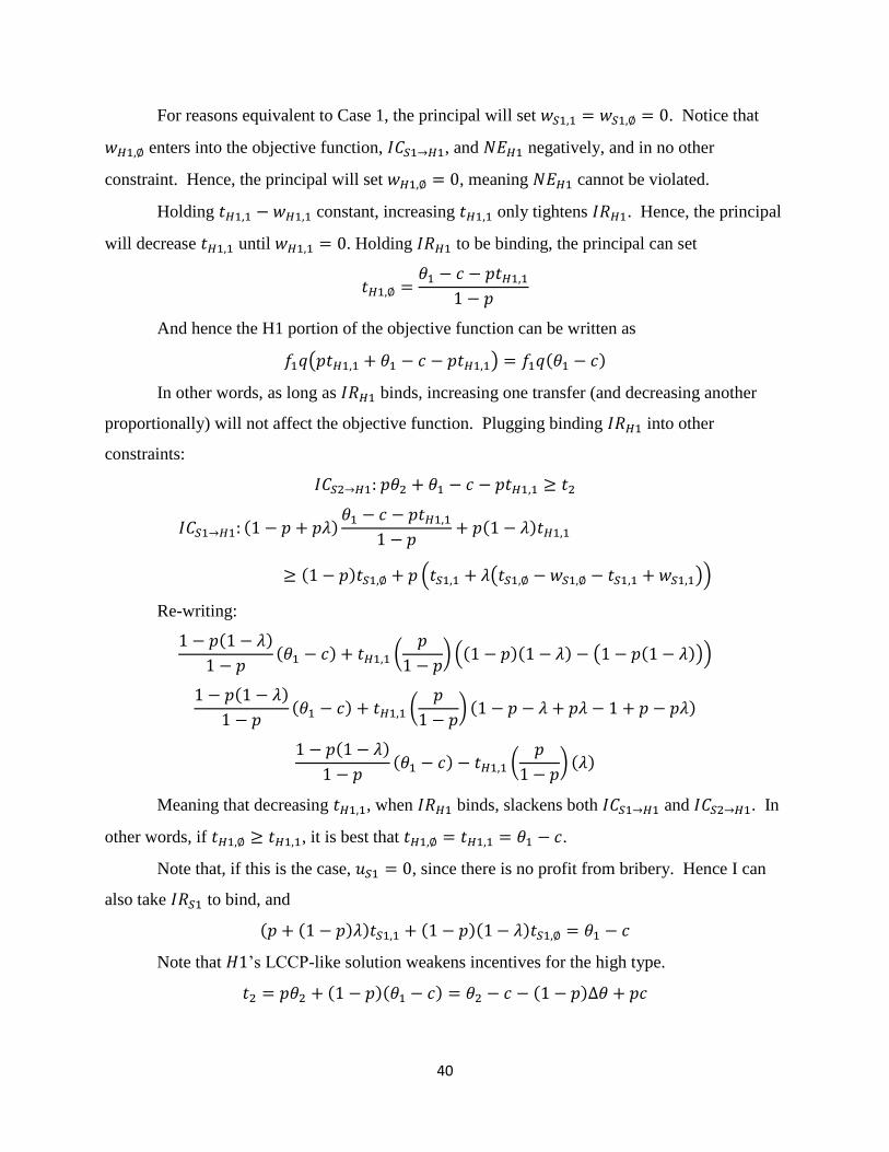
For reasons equivalent to Case 1, the principal will set 𝑤𝑆1,1 = 𝑤𝑆1,∅ = 0. Notice that

𝑤𝐻1,∅ enters into the objective function, 𝐼𝐶𝑆1→𝐻1, and 𝑁𝐸𝐻1 negatively, and in no other

constraint. Hence, the principal will set 𝑤𝐻1,∅ = 0, meaning 𝑁𝐸𝐻1 cannot be violated.

Holding 𝑡𝐻1,1 − 𝑤𝐻1,1 constant, increasing 𝑡𝐻1,1 only tightens 𝐼𝑅𝐻1. Hence, the principal

will decrease 𝑡𝐻1,1 until 𝑤𝐻1,1 = 0. Holding 𝐼𝑅𝐻1 to be binding, the principal can set

𝑡𝐻1,∅ =𝜃1 − 𝑐 − 𝑝𝑡𝐻1,1

1 − 𝑝

And hence the H1 portion of the objective function can be written as

𝑓1𝑞(𝑝𝑡𝐻1,1 + 𝜃1 − 𝑐 − 𝑝𝑡𝐻1,1) = 𝑓1𝑞(𝜃1 − 𝑐)

In other words, as long as 𝐼𝑅𝐻1 binds, increasing one transfer (and decreasing another

proportionally) will not affect the objective function. Plugging binding 𝐼𝑅𝐻1 into other

constraints:

𝐼𝐶𝑆2→𝐻1: 𝑝𝜃2 + 𝜃1 − 𝑐 − 𝑝𝑡𝐻1,1 ≥ 𝑡2

𝐼𝐶𝑆1→𝐻1: (1 − 𝑝 + 𝑝𝜆)𝜃1 − 𝑐 − 𝑝𝑡𝐻1,1

1 − 𝑝+ 𝑝(1 − 𝜆)𝑡𝐻1,1

≥ (1 − 𝑝)𝑡𝑆1,∅ + 𝑝 (𝑡𝑆1,1 + 𝜆(𝑡𝑆1,∅ − 𝑤𝑆1,∅ − 𝑡𝑆1,1 + 𝑤𝑆1,1))

Re-writing:

1 − 𝑝(1 − 𝜆)

1 − 𝑝(𝜃1 − 𝑐) + 𝑡𝐻1,1 (

𝑝

1 − 𝑝) ((1 − 𝑝)(1 − 𝜆) − (1 − 𝑝(1 − 𝜆)))

1 − 𝑝(1 − 𝜆)

1 − 𝑝(𝜃1 − 𝑐) + 𝑡𝐻1,1 (

𝑝

1 − 𝑝) (1 − 𝑝 − 𝜆 + 𝑝𝜆 − 1 + 𝑝 − 𝑝𝜆)

1 − 𝑝(1 − 𝜆)

1 − 𝑝(𝜃1 − 𝑐) − 𝑡𝐻1,1 (

𝑝

1 − 𝑝) (𝜆)

Meaning that decreasing 𝑡𝐻1,1, when 𝐼𝑅𝐻1 binds, slackens both 𝐼𝐶𝑆1→𝐻1 and 𝐼𝐶𝑆2→𝐻1. In

other words, if 𝑡𝐻1,∅ ≥ 𝑡𝐻1,1, it is best that 𝑡𝐻1,∅ = 𝑡𝐻1,1 = 𝜃1 − 𝑐.

Note that, if this is the case, 𝑢𝑆1 = 0, since there is no profit from bribery. Hence I can

also take 𝐼𝑅𝑆1 to bind, and

(𝑝 + (1 − 𝑝)𝜆)𝑡𝑆1,1 + (1 − 𝑝)(1 − 𝜆)𝑡𝑆1,∅ = 𝜃1 − 𝑐

Note that 𝐻1’s LCCP-like solution weakens incentives for the high type.

𝑡2 = 𝑝𝜃2 + (1 − 𝑝)(𝜃1 − 𝑐) = 𝜃2 − 𝑐 − (1 − 𝑝)Δ𝜃 + 𝑝𝑐

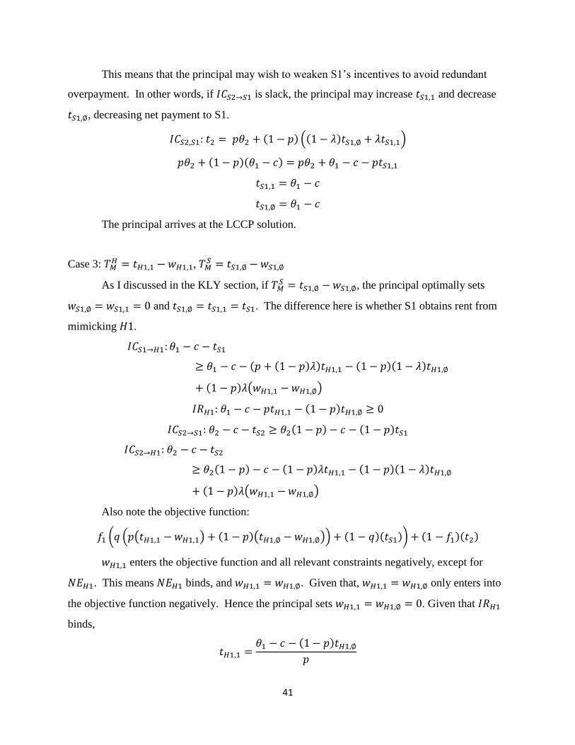
41

This means that the principal may wish to weaken S1’s incentives to avoid redundant

overpayment. In other words, if 𝐼𝐶𝑆2→𝑆1 is slack, the principal may increase 𝑡𝑆1,1 and decrease

𝑡𝑆1,∅, decreasing net payment to S1.

𝐼𝐶𝑆2,𝑆1: 𝑡2 = 𝑝𝜃2 + (1 − 𝑝) ((1 − 𝜆)𝑡𝑆1,∅ + 𝜆𝑡𝑆1,1)

𝑝𝜃2 + (1 − 𝑝)(𝜃1 − 𝑐) = 𝑝𝜃2 + 𝜃1 − 𝑐 − 𝑝𝑡𝑆1,1

𝑡𝑆1,1 = 𝜃1 − 𝑐

𝑡𝑆1,∅ = 𝜃1 − 𝑐

The principal arrives at the LCCP solution.

Case 3: 𝑇𝑀𝐻 = 𝑡𝐻1,1 − 𝑤𝐻1,1, 𝑇𝑀

𝑆 = 𝑡𝑆1,∅ − 𝑤𝑆1,∅

As I discussed in the KLY section, if 𝑇𝑀𝑆 = 𝑡𝑆1,∅ − 𝑤𝑆1,∅, the principal optimally sets

𝑤𝑆1,∅ = 𝑤𝑆1,1 = 0 and 𝑡𝑆1,∅ = 𝑡𝑆1,1 = 𝑡𝑆1. The difference here is whether S1 obtains rent from

mimicking 𝐻1.

𝐼𝐶𝑆1→𝐻1: 𝜃1 − 𝑐 − 𝑡𝑆1

≥ 𝜃1 − 𝑐 − (𝑝 + (1 − 𝑝)𝜆)𝑡𝐻1,1 − (1 − 𝑝)(1 − 𝜆)𝑡𝐻1,∅

+ (1 − 𝑝)𝜆(𝑤𝐻1,1 − 𝑤𝐻1,∅)

𝐼𝑅𝐻1: 𝜃1 − 𝑐 − 𝑝𝑡𝐻1,1 − (1 − 𝑝)𝑡𝐻1,∅ ≥ 0

𝐼𝐶𝑆2→𝑆1: 𝜃2 − 𝑐 − 𝑡𝑆2 ≥ 𝜃2(1 − 𝑝) − 𝑐 − (1 − 𝑝)𝑡𝑆1

𝐼𝐶𝑆2→𝐻1: 𝜃2 − 𝑐 − 𝑡𝑆2

≥ 𝜃2(1 − 𝑝) − 𝑐 − (1 − 𝑝)𝜆𝑡𝐻1,1 − (1 − 𝑝)(1 − 𝜆)𝑡𝐻1,∅

+ (1 − 𝑝)𝜆(𝑤𝐻1,1 − 𝑤𝐻1,∅)

Also note the objective function:

𝑓1 (𝑞 (𝑝(𝑡𝐻1,1 − 𝑤𝐻1,1) + (1 − 𝑝)(𝑡𝐻1,∅ − 𝑤𝐻1,∅)) + (1 − 𝑞)(𝑡𝑆1)) + (1 − 𝑓1)(𝑡2)

𝑤𝐻1,1 enters the objective function and all relevant constraints negatively, except for

𝑁𝐸𝐻1. This means 𝑁𝐸𝐻1 binds, and 𝑤𝐻1,1 = 𝑤𝐻1,∅. Given that, 𝑤𝐻1,1 = 𝑤𝐻1,∅ only enters into

the objective function negatively. Hence the principal sets 𝑤𝐻1,1 = 𝑤𝐻1,∅ = 0. Given that 𝐼𝑅𝐻1

binds,

𝑡𝐻1,1 =𝜃1 − 𝑐 − (1 − 𝑝)𝑡𝐻1,∅

𝑝

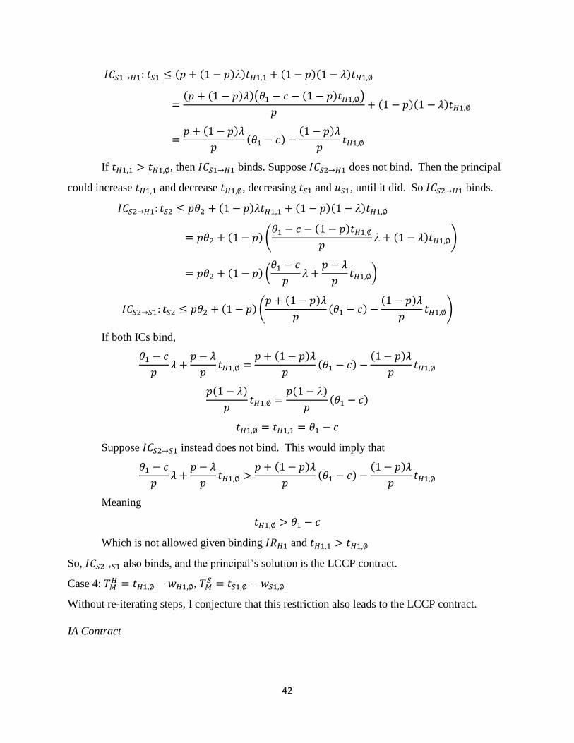
42

𝐼𝐶𝑆1→𝐻1: 𝑡𝑆1 ≤ (𝑝 + (1 − 𝑝)𝜆)𝑡𝐻1,1 + (1 − 𝑝)(1 − 𝜆)𝑡𝐻1,∅

=(𝑝 + (1 − 𝑝)𝜆)(𝜃1 − 𝑐 − (1 − 𝑝)𝑡𝐻1,∅)

𝑝+ (1 − 𝑝)(1 − 𝜆)𝑡𝐻1,∅

=𝑝 + (1 − 𝑝)𝜆

𝑝(𝜃1 − 𝑐) −

(1 − 𝑝)𝜆

𝑝𝑡𝐻1,∅

If 𝑡𝐻1,1 > 𝑡𝐻1,∅, then 𝐼𝐶𝑆1→𝐻1 binds. Suppose 𝐼𝐶𝑆2→𝐻1 does not bind. Then the principal

could increase 𝑡𝐻1,1 and decrease 𝑡𝐻1,∅, decreasing 𝑡𝑆1 and 𝑢𝑆1, until it did. So 𝐼𝐶𝑆2→𝐻1 binds.

𝐼𝐶𝑆2→𝐻1: 𝑡𝑆2 ≤ 𝑝𝜃2 + (1 − 𝑝)𝜆𝑡𝐻1,1 + (1 − 𝑝)(1 − 𝜆)𝑡𝐻1,∅

= 𝑝𝜃2 + (1 − 𝑝) (𝜃1 − 𝑐 − (1 − 𝑝)𝑡𝐻1,∅

𝑝𝜆 + (1 − 𝜆)𝑡𝐻1,∅)

= 𝑝𝜃2 + (1 − 𝑝) (𝜃1 − 𝑐

𝑝𝜆 +

𝑝 − 𝜆

𝑝𝑡𝐻1,∅)

𝐼𝐶𝑆2→𝑆1: 𝑡𝑆2 ≤ 𝑝𝜃2 + (1 − 𝑝) (𝑝 + (1 − 𝑝)𝜆

𝑝(𝜃1 − 𝑐) −

(1 − 𝑝)𝜆

𝑝𝑡𝐻1,∅)

If both ICs bind,

𝜃1 − 𝑐

𝑝𝜆 +

𝑝 − 𝜆

𝑝𝑡𝐻1,∅ =

𝑝 + (1 − 𝑝)𝜆

𝑝(𝜃1 − 𝑐) −

(1 − 𝑝)𝜆

𝑝𝑡𝐻1,∅

𝑝(1 − 𝜆)

𝑝𝑡𝐻1,∅ =

𝑝(1 − 𝜆)

𝑝(𝜃1 − 𝑐)

𝑡𝐻1,∅ = 𝑡𝐻1,1 = 𝜃1 − 𝑐

Suppose 𝐼𝐶𝑆2→𝑆1 instead does not bind. This would imply that

𝜃1 − 𝑐

𝑝𝜆 +

𝑝 − 𝜆

𝑝𝑡𝐻1,∅ >

𝑝 + (1 − 𝑝)𝜆

𝑝(𝜃1 − 𝑐) −

(1 − 𝑝)𝜆

𝑝𝑡𝐻1,∅

Meaning

𝑡𝐻1,∅ > 𝜃1 − 𝑐

Which is not allowed given binding 𝐼𝑅𝐻1 and 𝑡𝐻1,1 > 𝑡𝐻1,∅

So, 𝐼𝐶𝑆2→𝑆1 also binds, and the principal’s solution is the LCCP contract.

Case 4: 𝑇𝑀𝐻 = 𝑡𝐻1,∅ − 𝑤𝐻1,∅, 𝑇𝑀

𝑆 = 𝑡𝑆1,∅ − 𝑤𝑆1,∅

Without re-iterating steps, I conjecture that this restriction also leads to the LCCP contract.

IA Contract

43

For brevity I assert that the logic has not changed from the previous contracts for the following

results for both 𝐻 and 𝑆:

𝑡12 = 𝜃2

𝑤12 = 𝜃2 + 𝑇𝑀

𝑤11 = 𝑤1∅ = 0

Case 1: 𝑇𝑀𝐻 = 𝑡𝐻1,1 − 𝑤𝐻1,1; 𝑇𝑀

𝑆 = 𝑡𝑆1,1 − 𝑤𝑆1,1

Using the same logic as in the INA contract we can conclude that 𝑡𝐻1,1 = 𝑡𝑆1,1 = 𝑡1,1 and

𝑡𝐻1,∅ = 𝑡𝑆1,∅ = 𝑡1,∅, and we have determined that 𝑡𝐻2 = 𝑡𝑆2,∅.

max𝑡𝑖,𝑤𝑖

𝑓1(𝑞(𝑝𝑡1,1 + (1 − 𝑝)𝑡1,∅) + (1 − 𝑞)𝑡1,1) + (1 − 𝑓1) (𝑞(𝑡𝑆2,∅) + (1 − 𝑞)(𝑡𝑆2,2))

s.t.

𝐼𝑅𝐻1: 𝜃1 − 𝑐 − 𝑝𝑡1,1 − (1 − 𝑝)𝑡1,∅ ≥ 0

𝐼𝐶𝑆2→𝐻1: 𝜃2 − 𝑐 − (1 − 𝜆)𝑡𝑆2,∅ − 𝜆𝑡𝑆2,2 ≥ 𝜃2(1 − 𝑝) − 𝑐 − (1 − 𝑝)(𝜆𝑡1,1 + (1 − 𝜆)𝑡1,∅)

𝐼𝐶𝐻2→𝐻1: 𝜃2 − 𝑐 − 𝑡𝑆2,∅ ≥ 𝜃2(1 − 𝑝) − 𝑐 − (1 − 𝑝)𝑡1,∅

𝐿𝐿𝐶1,∅: 𝜃1 − 𝑡1,∅ ≥ 0

Since it is established that 𝑞 > 1 − 𝜆 and 𝑐 ≤ Δ𝜃(1 − 𝑝) we know that all of the above

constraints bind as long as 𝐿𝐿𝐶1,∅ binds. So we can solve:

max𝑡𝑖,𝑤𝑖

𝐿 = 𝑓1(𝑞(𝑝𝑡1,1 + (1 − 𝑝)𝑡1,∅) + (1 − 𝑞)𝑡1,1) + (1 − 𝑓1) (𝑞(𝑡𝑆2,∅) + (1 − 𝑞)(𝑡𝑆2,2))

+𝜙1(𝜃1 − 𝑐 − 𝑝𝑡1,1 − (1 − 𝑝)𝑡1,∅)

+𝜙2 (𝜃2 − 𝑐 − (1 − 𝜆)𝑡𝑆2,∅ − 𝜆𝑡𝑆2,2 − 𝜃2(1 − 𝑝) + 𝑐 + (1 − 𝑝)(𝜆𝑡1,1 + (1 − 𝜆)𝑡1,∅))

+𝜙3(𝜃2 − 𝑐 − 𝑡𝑆2,∅ − 𝜃2(1 − 𝑝) + 𝑐 + (1 − 𝑝)𝑡1,∅)

+𝜙4(𝜃1 − 𝑡1,∅)

First order conditions:

[𝑡1,1]: 𝑓1(𝑞𝑝 + (1 − 𝑞)) − 𝜙1𝑝 + 𝜙2(1 − 𝑝) = 0

[𝑡1,∅]: 𝑓1𝑞(1 − 𝑝) − 𝜙1(1 − 𝑝) + 𝜙2(1 − 𝑝)(1 − 𝜆) + 𝜙3(1 − 𝑝) − 𝜙4 = 0

[𝑡𝑆2,∅]: (1 − 𝑓1)𝑞 − 𝜙2(1 − 𝜆) − 𝜙3 = 0

[𝑡𝑆2,2]: (1 − 𝑓1)(1 − 𝑞) − 𝜙2𝜆 = 0

Solving:

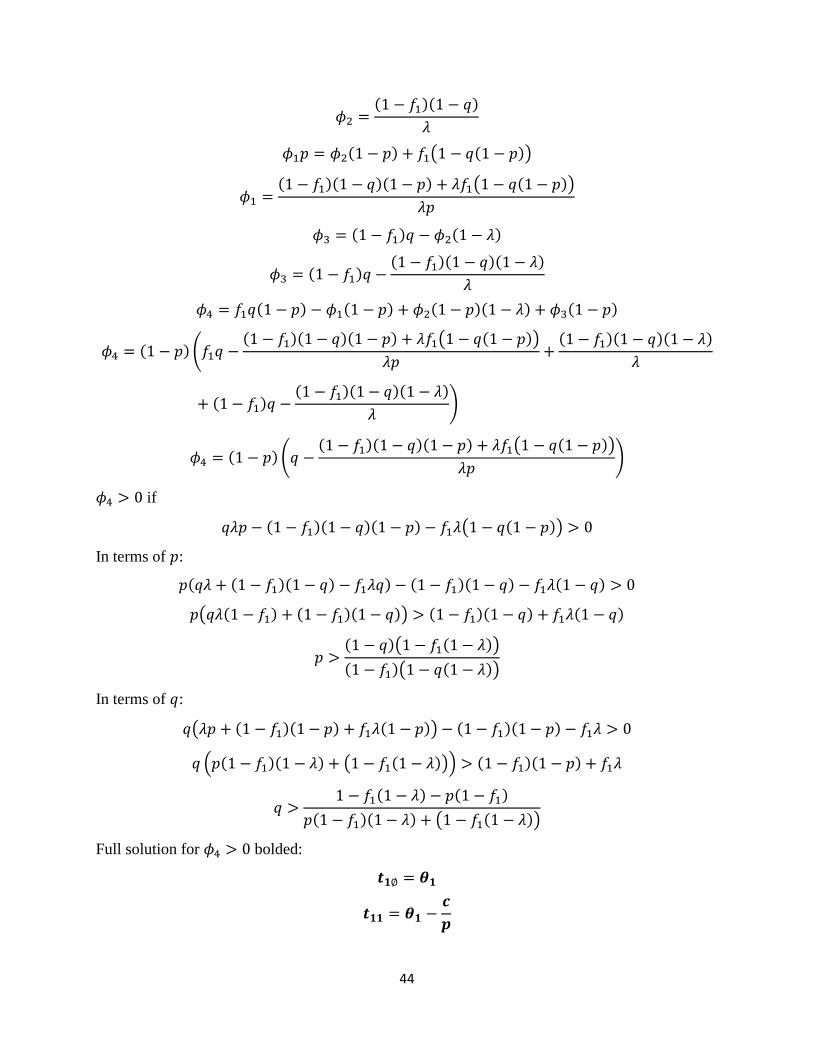
44

𝜙2 =(1 − 𝑓1)(1 − 𝑞)

𝜆

𝜙1𝑝 = 𝜙2(1 − 𝑝) + 𝑓1(1 − 𝑞(1 − 𝑝))

𝜙1 =(1 − 𝑓1)(1 − 𝑞)(1 − 𝑝) + 𝜆𝑓1(1 − 𝑞(1 − 𝑝))

𝜆𝑝

𝜙3 = (1 − 𝑓1)𝑞 − 𝜙2(1 − 𝜆)

𝜙3 = (1 − 𝑓1)𝑞 −(1 − 𝑓1)(1 − 𝑞)(1 − 𝜆)

𝜆

𝜙4 = 𝑓1𝑞(1 − 𝑝) − 𝜙1(1 − 𝑝) + 𝜙2(1 − 𝑝)(1 − 𝜆) + 𝜙3(1 − 𝑝)

𝜙4 = (1 − 𝑝) (𝑓1𝑞 −(1 − 𝑓1)(1 − 𝑞)(1 − 𝑝) + 𝜆𝑓1(1 − 𝑞(1 − 𝑝))

𝜆𝑝+

(1 − 𝑓1)(1 − 𝑞)(1 − 𝜆)

𝜆

+ (1 − 𝑓1)𝑞 −(1 − 𝑓1)(1 − 𝑞)(1 − 𝜆)

𝜆)

𝜙4 = (1 − 𝑝) (𝑞 −(1 − 𝑓1)(1 − 𝑞)(1 − 𝑝) + 𝜆𝑓1(1 − 𝑞(1 − 𝑝))

𝜆𝑝)

𝜙4 > 0 if

𝑞𝜆𝑝 − (1 − 𝑓1)(1 − 𝑞)(1 − 𝑝) − 𝑓1𝜆(1 − 𝑞(1 − 𝑝)) > 0

In terms of 𝑝:

𝑝(𝑞𝜆 + (1 − 𝑓1)(1 − 𝑞) − 𝑓1𝜆𝑞) − (1 − 𝑓1)(1 − 𝑞) − 𝑓1𝜆(1 − 𝑞) > 0

𝑝(𝑞𝜆(1 − 𝑓1) + (1 − 𝑓1)(1 − 𝑞)) > (1 − 𝑓1)(1 − 𝑞) + 𝑓1𝜆(1 − 𝑞)

𝑝 >(1 − 𝑞)(1 − 𝑓1(1 − 𝜆))

(1 − 𝑓1)(1 − 𝑞(1 − 𝜆))

In terms of 𝑞:

𝑞(𝜆𝑝 + (1 − 𝑓1)(1 − 𝑝) + 𝑓1𝜆(1 − 𝑝)) − (1 − 𝑓1)(1 − 𝑝) − 𝑓1𝜆 > 0

𝑞 (𝑝(1 − 𝑓1)(1 − 𝜆) + (1 − 𝑓1(1 − 𝜆))) > (1 − 𝑓1)(1 − 𝑝) + 𝑓1𝜆

𝑞 >1 − 𝑓1(1 − 𝜆) − 𝑝(1 − 𝑓1)

𝑝(1 − 𝑓1)(1 − 𝜆) + (1 − 𝑓1(1 − 𝜆))

Full solution for 𝜙4 > 0 bolded:

𝒕𝟏∅ = 𝜽𝟏

𝒕𝟏𝟏 = 𝜽𝟏 −𝒄

𝒑

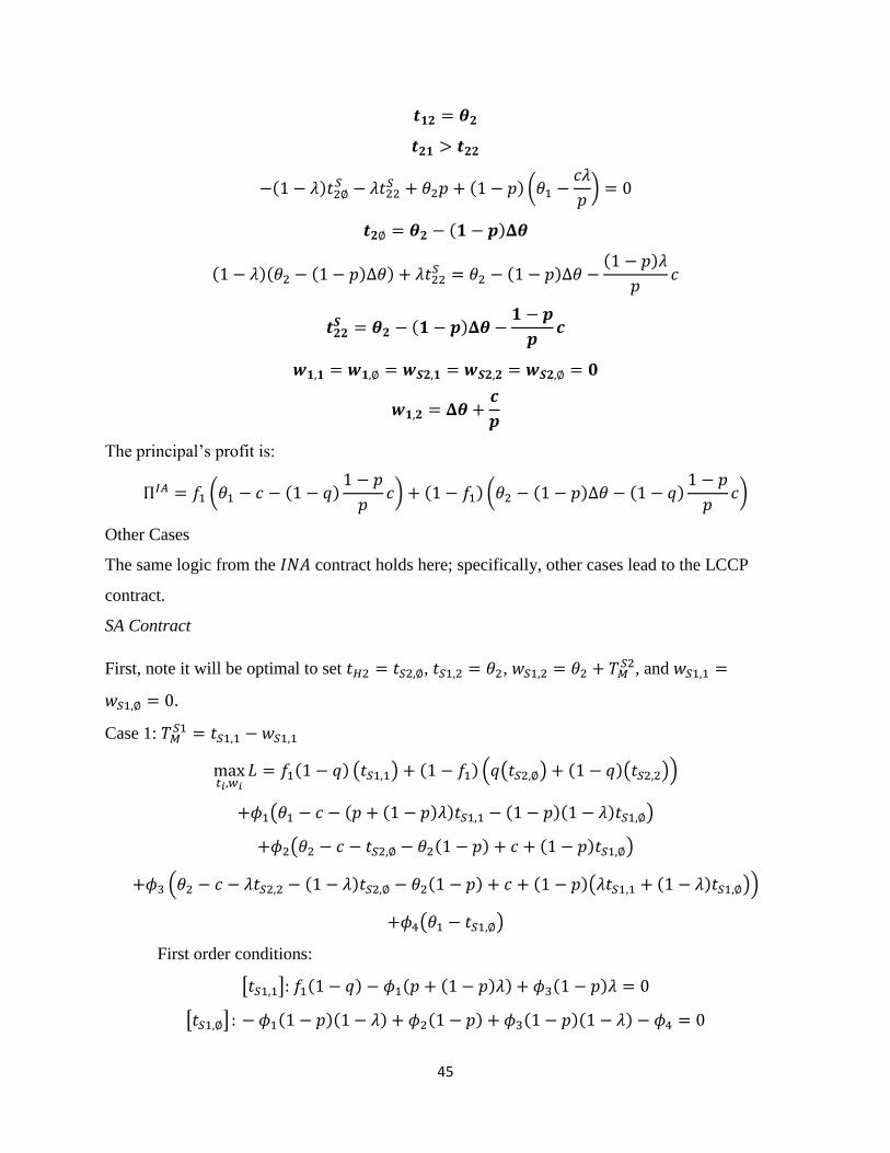
45

𝒕𝟏𝟐 = 𝜽𝟐

𝒕𝟐𝟏 > 𝒕𝟐𝟐

−(1 − 𝜆)𝑡2∅𝑆 − 𝜆𝑡22

𝑆 + 𝜃2𝑝 + (1 − 𝑝) (𝜃1 −𝑐𝜆

𝑝) = 0

𝒕𝟐∅ = 𝜽𝟐 − (𝟏 − 𝒑)𝚫𝜽

(1 − 𝜆)(𝜃2 − (1 − 𝑝)Δ𝜃) + 𝜆𝑡22𝑆 = 𝜃2 − (1 − 𝑝)Δ𝜃 −

(1 − 𝑝)𝜆

𝑝𝑐

𝒕𝟐𝟐𝑺 = 𝜽𝟐 − (𝟏 − 𝒑)𝚫𝜽 −

𝟏 − 𝒑

𝒑𝒄

𝒘𝟏,𝟏 = 𝒘𝟏,∅ = 𝒘𝑺𝟐,𝟏 = 𝒘𝑺𝟐,𝟐 = 𝒘𝑺𝟐,∅ = 𝟎

𝒘𝟏,𝟐 = 𝚫𝜽 +𝒄

𝒑

The principal’s profit is:

Π𝐼𝐴 = 𝑓1 (𝜃1 − 𝑐 − (1 − 𝑞)1 − 𝑝

𝑝𝑐) + (1 − 𝑓1) (𝜃2 − (1 − 𝑝)Δ𝜃 − (1 − 𝑞)

1 − 𝑝

𝑝𝑐)

Other Cases

The same logic from the 𝐼𝑁𝐴 contract holds here; specifically, other cases lead to the LCCP

contract.

SA Contract

First, note it will be optimal to set 𝑡𝐻2 = 𝑡𝑆2,∅, 𝑡𝑆1,2 = 𝜃2, 𝑤𝑆1,2 = 𝜃2 + 𝑇𝑀𝑆2, and 𝑤𝑆1,1 =

𝑤𝑆1,∅ = 0.

Case 1: 𝑇𝑀𝑆1 = 𝑡𝑆1,1 − 𝑤𝑆1,1

max𝑡𝑖,𝑤𝑖

𝐿 = 𝑓1(1 − 𝑞) (𝑡𝑆1,1) + (1 − 𝑓1) (𝑞(𝑡𝑆2,∅) + (1 − 𝑞)(𝑡𝑆2,2))

+𝜙1(𝜃1 − 𝑐 − (𝑝 + (1 − 𝑝)𝜆)𝑡𝑆1,1 − (1 − 𝑝)(1 − 𝜆)𝑡𝑆1,∅)

+𝜙2(𝜃2 − 𝑐 − 𝑡𝑆2,∅ − 𝜃2(1 − 𝑝) + 𝑐 + (1 − 𝑝)𝑡𝑆1,∅)

+𝜙3 (𝜃2 − 𝑐 − 𝜆𝑡𝑆2,2 − (1 − 𝜆)𝑡𝑆2,∅ − 𝜃2(1 − 𝑝) + 𝑐 + (1 − 𝑝)(𝜆𝑡𝑆1,1 + (1 − 𝜆)𝑡𝑆1,∅))

+𝜙4(𝜃1 − 𝑡𝑆1,∅)

First order conditions:

[𝑡𝑆1,1]: 𝑓1(1 − 𝑞) − 𝜙1(𝑝 + (1 − 𝑝)𝜆) + 𝜙3(1 − 𝑝)𝜆 = 0

[𝑡𝑆1,∅] : − 𝜙1(1 − 𝑝)(1 − 𝜆) + 𝜙2(1 − 𝑝) + 𝜙3(1 − 𝑝)(1 − 𝜆) − 𝜙4 = 0

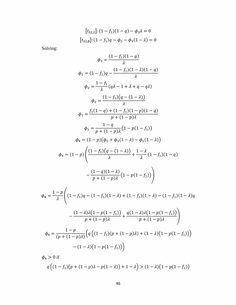
46

[𝑡𝑆2,2]: (1 − 𝑓1)(1 − 𝑞) − 𝜙3𝜆 = 0

[𝑡𝑆2,∅]: (1 − 𝑓1)𝑞 − 𝜙2 − 𝜙3(1 − 𝜆) = 0

Solving:

𝜙3 =(1 − 𝑓1)(1 − 𝑞)

𝜆

𝜙2 = (1 − 𝑓1)𝑞 −(1 − 𝑓1)(1 − 𝜆)(1 − 𝑞)

𝜆

𝜙2 =1 − 𝑓1

𝜆(𝑞𝜆 − 1 + 𝜆 + 𝑞 − 𝑞𝜆)

𝜙2 =(1 − 𝑓1)(𝑞 − (1 − 𝜆))

𝜆

𝜙1 =𝑓1(1 − 𝑞) + (1 − 𝑓1)(1 − 𝑝)(1 − 𝑞)

𝑝 + (1 − 𝑝)𝜆

𝜙1 =1 − 𝑞

𝑝 + (1 − 𝑝)𝜆(1 − 𝑝(1 − 𝑓1))

𝜙4 = (1 − 𝑝)(𝜙2 + 𝜙3(1 − 𝜆) − 𝜙1(1 − 𝜆))

𝜙4 = (1 − 𝑝) ((1 − 𝑓1)(𝑞 − (1 − 𝜆))

𝜆+

1 − 𝜆

𝜆(1 − 𝑓1)(1 − 𝑞)

−(1 − 𝑞)(1 − 𝜆)

𝑝 + (1 − 𝑝)𝜆(1 − 𝑝(1 − 𝑓1)))

𝜙4 =1 − 𝑝

𝜆((1 − 𝑓1)𝑞 − (1 − 𝑓1)(1 − 𝜆) + (1 − 𝑓1)(1 − 𝜆) − (1 − 𝑓1)(1 − 𝜆)𝑞

−(1 − 𝜆)𝜆(1 − 𝑝(1 − 𝑓1))

𝑝 + (1 − 𝑝)𝜆+

𝑞(1 − 𝜆)𝜆(1 − 𝑝(1 − 𝑓1))

𝑝 + (1 − 𝑝)𝜆)

𝜙4 =1 − 𝑝

(𝑝 + (1 − 𝑝)𝜆)(𝑞 ((1 − 𝑓1)(𝑝 + (1 − 𝑝)𝜆) + (1 − 𝜆)(1 − 𝑝(1 − 𝑓1)))

− (1 − 𝜆)(1 − 𝑝(1 − 𝑓1)))

𝜙4 > 0 if

𝑞 ((1 − 𝑓1)(𝑝 + (1 − 𝑝)𝜆 − 𝑝(1 − 𝜆)) + 1 − 𝜆) > (1 − 𝜆)(1 − 𝑝(1 − 𝑓1))

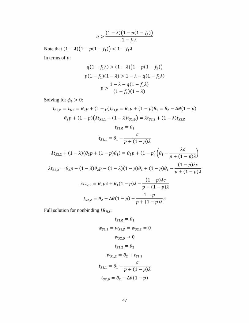
47

𝑞 >(1 − 𝜆)(1 − 𝑝(1 − 𝑓1))

1 − 𝑓1𝜆

Note that (1 − 𝜆)(1 − 𝑝(1 − 𝑓1)) < 1 − 𝑓1𝜆

In terms of 𝑝:

𝑞(1 − 𝑓1𝜆) > (1 − 𝜆)(1 − 𝑝(1 − 𝑓1))

𝑝(1 − 𝑓1)(1 − 𝜆) > 1 − 𝜆 − 𝑞(1 − 𝑓1𝜆)

𝑝 >1 − 𝜆 − 𝑞(1 − 𝑓1𝜆)

(1 − 𝑓1)(1 − 𝜆)

Solving for 𝜙4 > 0:

𝑡𝑆2,∅ = 𝑡𝐻2 = 𝜃2𝑝 + (1 − 𝑝)𝑡𝑆1,∅ = 𝜃2𝑝 + (1 − 𝑝)𝜃1 = 𝜃2 − Δ𝜃(1 − 𝑝)

𝜃2𝑝 + (1 − 𝑝)(𝜆𝑡𝑆1,1 + (1 − 𝜆)𝑡𝑆1,∅) = 𝜆𝑡𝑆2,2 + (1 − 𝜆)𝑡𝑆2,∅

𝑡𝑆1,∅ = 𝜃1

𝑡𝑆1,1 = 𝜃1 −𝑐

𝑝 + (1 − 𝑝)𝜆

𝜆𝑡𝑆2,2 + (1 − 𝜆)(𝜃2𝑝 + (1 − 𝑝)𝜃1) = 𝜃2𝑝 + (1 − 𝑝) (𝜃1 −𝜆𝑐

𝑝 + (1 − 𝑝)𝜆)

𝜆𝑡𝑆2,2 = 𝜃2𝑝 − (1 − 𝜆)𝜃2𝑝 − (1 − 𝜆)(1 − 𝑝)𝜃1 + (1 − 𝑝)𝜃1 −(1 − 𝑝)𝜆𝑐

𝑝 + (1 − 𝑝)𝜆

𝜆𝑡𝑆2,2 = 𝜃2𝑝𝜆 + 𝜃1(1 − 𝑝)𝜆 −(1 − 𝑝)𝜆𝑐

𝑝 + (1 − 𝑝)𝜆

𝑡𝑆2,2 = 𝜃2 − Δ𝜃(1 − 𝑝) −1 − 𝑝

𝑝 + (1 − 𝑝)𝜆𝑐

Full solution for nonbinding 𝐼𝑅𝐻2:

𝑡𝑆1,∅ = 𝜃1

𝑤𝑆1,1 = 𝑤𝑆1,∅ = 𝑤𝑆2,2 = 0

𝑤𝑆2,∅ → 0

𝑡𝑆1,2 = 𝜃2

𝑤𝑆1,2 = 𝜃2 + 𝑡𝑆1,1

𝑡𝑆1,1 = 𝜃1 −𝑐

𝑝 + (1 − 𝑝)𝜆

𝑡𝑆2,∅ = 𝜃2 − Δ𝜃(1 − 𝑝)

48

𝑡𝑆2,2 = 𝜃2 − Δ𝜃(1 − 𝑝) −1 − 𝑝

𝑝 + (1 − 𝑝)𝜆𝑐

Profit for SA:

Π𝑆𝐴 = 𝑓1(1 − 𝑞) (𝜃1 −𝑐

𝑝 + (1 − 𝑝)𝜆) + (1 − 𝑓1) (𝜃2 − Δ𝜃(1 − 𝑝) −

(1 − 𝑞)(1 − 𝑝)

𝑝 + (1 − 𝑝)𝜆𝑐)

Other cases:

This follows the logic of the SNA contract and KLY contract; specifically, other cases would

lead to the LCCP contract.

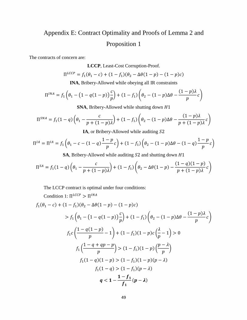
49

Appendix E: Contract Optimality and Proofs of Lemma 2 and

Proposition 1

The contracts of concern are:

LCCP, Least-Cost Corruption-Proof.

Π𝐿𝐶𝐶𝑃 = 𝑓1(𝜃1 − 𝑐) + (1 − 𝑓1)(𝜃2 − Δ𝜃(1 − 𝑝) − (1 − 𝑝)𝑐)

INA, Bribery-Allowed while obeying all IR constraints

Π𝐼𝑁𝐴 = 𝑓1 (𝜃1 − (1 − 𝑞(1 − 𝑝))𝑐

𝑝) + (1 − 𝑓1) (𝜃2 − (1 − 𝑝)Δ𝜃 −

(1 − 𝑝)𝜆

𝑝𝑐)

SNA, Bribery-Allowed while shutting down 𝐻1

Π𝑆𝑁𝐴 = 𝑓1(1 − 𝑞) (𝜃1 −𝑐

𝑝 + (1 − 𝑝)𝜆) + (1 − 𝑓1) (𝜃2 − (1 − 𝑝)Δ𝜃 −

(1 − 𝑝)𝜆

𝑝 + (1 − 𝑝)𝜆𝑐)

IA, or Bribery-Allowed while auditing 𝑆2

Π𝐼𝐴 = Π𝐼𝐴 = 𝑓1 (𝜃1 − 𝑐 − (1 − 𝑞)1 − 𝑝

𝑝𝑐) + (1 − 𝑓1) (𝜃2 − (1 − 𝑝)Δ𝜃 − (1 − 𝑞)

1 − 𝑝

𝑝𝑐)

SA, Bribery-Allowed while auditing 𝑆2 and shutting down 𝐻1

Π𝑆𝐴 = 𝑓1(1 − 𝑞) (𝜃1 −𝑐

𝑝 + (1 − 𝑝)𝜆) + (1 − 𝑓1) (𝜃2 − Δ𝜃(1 − 𝑝) −

(1 − 𝑞)(1 − 𝑝)

𝑝 + (1 − 𝑝)𝜆𝑐)

The LCCP contract is optimal under four conditions:

Condition 1: Π𝐿𝐶𝐶𝑃 > Π𝐼𝑁𝐴

𝑓1(𝜃1 − 𝑐) + (1 − 𝑓1)(𝜃2 − Δ𝜃(1 − 𝑝) − (1 − 𝑝)𝑐)

> 𝑓1 (𝜃1 − (1 − 𝑞(1 − 𝑝))𝑐

𝑝) + (1 − 𝑓1) (𝜃2 − (1 − 𝑝)Δ𝜃 −

(1 − 𝑝)𝜆

𝑝𝑐)

𝑓1𝑐 (1 − 𝑞(1 − 𝑝)

𝑝− 1) + (1 − 𝑓1)(1 − 𝑝)𝑐 (

𝜆

𝑝− 1) > 0

𝑓1 (1 − 𝑞 + 𝑞𝑝 − 𝑝

𝑝) > (1 − 𝑓1)(1 − 𝑝) (

𝑝 − 𝜆

𝑝)

𝑓1(1 − 𝑞)(1 − 𝑝) > (1 − 𝑓1)(1 − 𝑝)(𝑝 − 𝜆)

𝑓1(1 − 𝑞) > (1 − 𝑓1)(𝑝 − 𝜆)

𝒒 < 𝟏 −𝟏 − 𝒇𝟏

𝒇𝟏

(𝒑 − 𝝀)

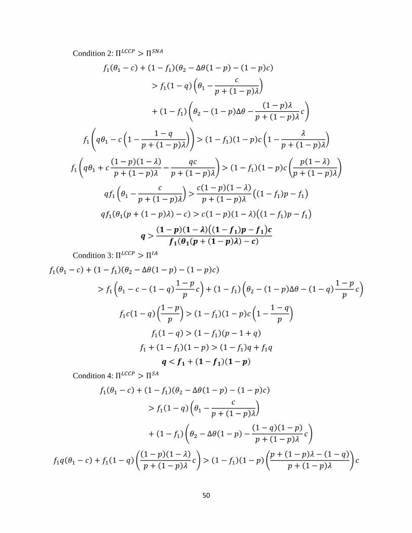
50

Condition 2: Π𝐿𝐶𝐶𝑃 > Π𝑆𝑁𝐴

𝑓1(𝜃1 − 𝑐) + (1 − 𝑓1)(𝜃2 − Δ𝜃(1 − 𝑝) − (1 − 𝑝)𝑐)

> 𝑓1(1 − 𝑞) (𝜃1 −𝑐

𝑝 + (1 − 𝑝)𝜆)

+ (1 − 𝑓1) (𝜃2 − (1 − 𝑝)Δ𝜃 −(1 − 𝑝)𝜆

𝑝 + (1 − 𝑝)𝜆𝑐)

𝑓1 (𝑞𝜃1 − 𝑐 (1 −1 − 𝑞

𝑝 + (1 − 𝑝)𝜆)) > (1 − 𝑓1)(1 − 𝑝)𝑐 (1 −

𝜆

𝑝 + (1 − 𝑝)𝜆)

𝑓1 (𝑞𝜃1 + 𝑐(1 − 𝑝)(1 − 𝜆)

𝑝 + (1 − 𝑝)𝜆−

𝑞𝑐

𝑝 + (1 − 𝑝)𝜆) > (1 − 𝑓1)(1 − 𝑝)𝑐 (

𝑝(1 − 𝜆)

𝑝 + (1 − 𝑝)𝜆)

𝑞𝑓1 (𝜃1 −𝑐

𝑝 + (1 − 𝑝)𝜆) >

𝑐(1 − 𝑝)(1 − 𝜆)

𝑝 + (1 − 𝑝)𝜆((1 − 𝑓1)𝑝 − 𝑓1)

𝑞𝑓1(𝜃1(𝑝 + (1 − 𝑝)𝜆) − 𝑐) > 𝑐(1 − 𝑝)(1 − 𝜆)((1 − 𝑓1)𝑝 − 𝑓1)

𝒒 >(𝟏 − 𝒑)(𝟏 − 𝝀)((𝟏 − 𝒇𝟏)𝒑 − 𝒇𝟏)𝒄

𝒇𝟏(𝜽𝟏(𝒑 + (𝟏 − 𝒑)𝝀) − 𝒄)

Condition 3: Π𝐿𝐶𝐶𝑃 > Π𝐼𝐴

𝑓1(𝜃1 − 𝑐) + (1 − 𝑓1)(𝜃2 − Δ𝜃(1 − 𝑝) − (1 − 𝑝)𝑐)

> 𝑓1 (𝜃1 − 𝑐 − (1 − 𝑞)1 − 𝑝

𝑝𝑐) + (1 − 𝑓1) (𝜃2 − (1 − 𝑝)Δ𝜃 − (1 − 𝑞)

1 − 𝑝

𝑝𝑐)

𝑓1𝑐(1 − 𝑞) (1 − 𝑝

𝑝) > (1 − 𝑓1)(1 − 𝑝)𝑐 (1 −

1 − 𝑞

𝑝)

𝑓1(1 − 𝑞) > (1 − 𝑓1)(𝑝 − 1 + 𝑞)

𝑓1 + (1 − 𝑓1)(1 − 𝑝) > (1 − 𝑓1)𝑞 + 𝑓1𝑞

𝒒 < 𝒇𝟏 + (𝟏 − 𝒇𝟏)(𝟏 − 𝒑)

Condition 4: Π𝐿𝐶𝐶𝑃 > Π𝑆𝐴

𝑓1(𝜃1 − 𝑐) + (1 − 𝑓1)(𝜃2 − Δ𝜃(1 − 𝑝) − (1 − 𝑝)𝑐)

> 𝑓1(1 − 𝑞) (𝜃1 −𝑐

𝑝 + (1 − 𝑝)𝜆)

+ (1 − 𝑓1) (𝜃2 − Δ𝜃(1 − 𝑝) −(1 − 𝑞)(1 − 𝑝)

𝑝 + (1 − 𝑝)𝜆𝑐)

𝑓1𝑞(𝜃1 − 𝑐) + 𝑓1(1 − 𝑞) ((1 − 𝑝)(1 − 𝜆)

𝑝 + (1 − 𝑝)𝜆𝑐) > (1 − 𝑓1)(1 − 𝑝) (

𝑝 + (1 − 𝑝)𝜆 − (1 − 𝑞)

𝑝 + (1 − 𝑝)𝜆) 𝑐

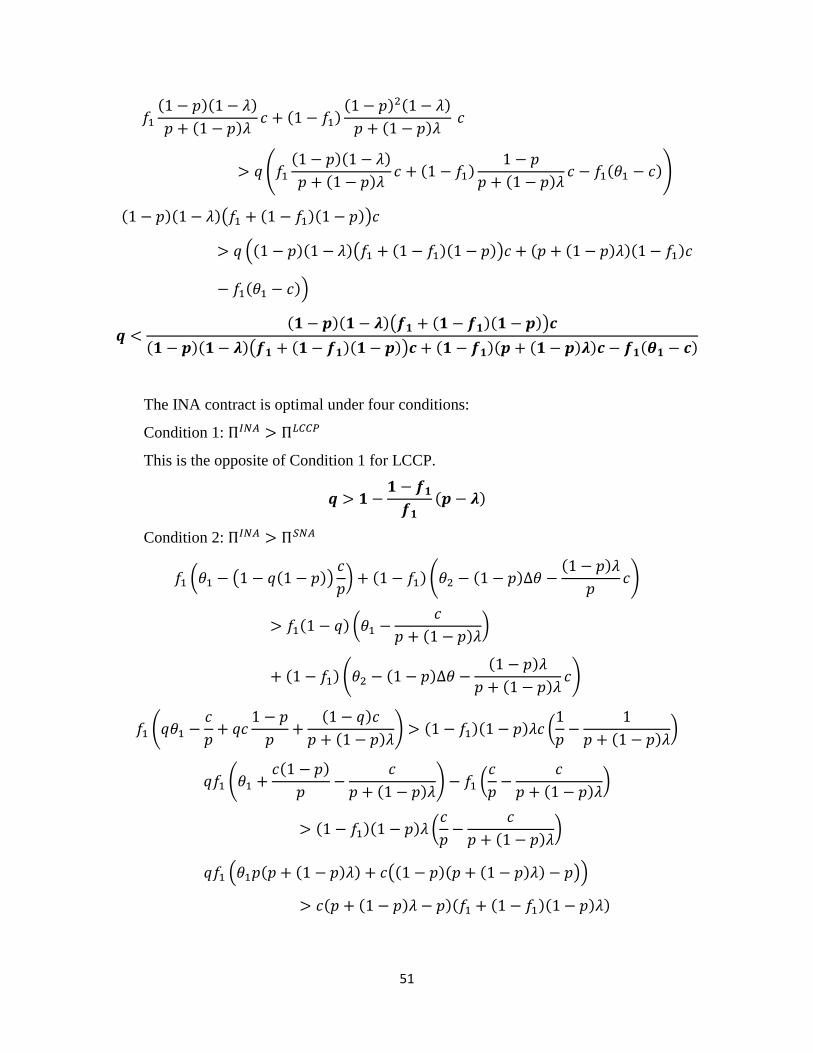
51

𝑓1

(1 − 𝑝)(1 − 𝜆)

𝑝 + (1 − 𝑝)𝜆𝑐 + (1 − 𝑓1)

(1 − 𝑝)2(1 − 𝜆)

𝑝 + (1 − 𝑝)𝜆 𝑐

> 𝑞 (𝑓1

(1 − 𝑝)(1 − 𝜆)

𝑝 + (1 − 𝑝)𝜆𝑐 + (1 − 𝑓1)

1 − 𝑝

𝑝 + (1 − 𝑝)𝜆𝑐 − 𝑓1(𝜃1 − 𝑐))

(1 − 𝑝)(1 − 𝜆)(𝑓1 + (1 − 𝑓1)(1 − 𝑝))𝑐

> 𝑞 ((1 − 𝑝)(1 − 𝜆)(𝑓1 + (1 − 𝑓1)(1 − 𝑝))𝑐 + (𝑝 + (1 − 𝑝)𝜆)(1 − 𝑓1)𝑐

− 𝑓1(𝜃1 − 𝑐))

𝒒 <(𝟏 − 𝒑)(𝟏 − 𝝀)(𝒇𝟏 + (𝟏 − 𝒇𝟏)(𝟏 − 𝒑))𝒄

(𝟏 − 𝒑)(𝟏 − 𝝀)(𝒇𝟏 + (𝟏 − 𝒇𝟏)(𝟏 − 𝒑))𝒄 + (𝟏 − 𝒇𝟏)(𝒑 + (𝟏 − 𝒑)𝝀)𝒄 − 𝒇𝟏(𝜽𝟏 − 𝒄)

The INA contract is optimal under four conditions:

Condition 1: Π𝐼𝑁𝐴 > Π𝐿𝐶𝐶𝑃

This is the opposite of Condition 1 for LCCP.

𝒒 > 𝟏 −𝟏 − 𝒇𝟏

𝒇𝟏

(𝒑 − 𝝀)

Condition 2: Π𝐼𝑁𝐴 > Π𝑆𝑁𝐴

𝑓1 (𝜃1 − (1 − 𝑞(1 − 𝑝))𝑐

𝑝) + (1 − 𝑓1) (𝜃2 − (1 − 𝑝)Δ𝜃 −

(1 − 𝑝)𝜆

𝑝𝑐)

> 𝑓1(1 − 𝑞) (𝜃1 −𝑐

𝑝 + (1 − 𝑝)𝜆)

+ (1 − 𝑓1) (𝜃2 − (1 − 𝑝)Δ𝜃 −(1 − 𝑝)𝜆

𝑝 + (1 − 𝑝)𝜆𝑐)

𝑓1 (𝑞𝜃1 −𝑐

𝑝+ 𝑞𝑐

1 − 𝑝

𝑝+

(1 − 𝑞)𝑐

𝑝 + (1 − 𝑝)𝜆) > (1 − 𝑓1)(1 − 𝑝)𝜆𝑐 (

1

𝑝−

1

𝑝 + (1 − 𝑝)𝜆)

𝑞𝑓1 (𝜃1 +𝑐(1 − 𝑝)

𝑝−

𝑐

𝑝 + (1 − 𝑝)𝜆) − 𝑓1 (

𝑐

𝑝−

𝑐

𝑝 + (1 − 𝑝)𝜆)

> (1 − 𝑓1)(1 − 𝑝)𝜆 (𝑐

𝑝−

𝑐

𝑝 + (1 − 𝑝)𝜆)

𝑞𝑓1 (𝜃1𝑝(𝑝 + (1 − 𝑝)𝜆) + 𝑐((1 − 𝑝)(𝑝 + (1 − 𝑝)𝜆) − 𝑝))

> 𝑐(𝑝 + (1 − 𝑝)𝜆 − 𝑝)(𝑓1 + (1 − 𝑓1)(1 − 𝑝)𝜆)

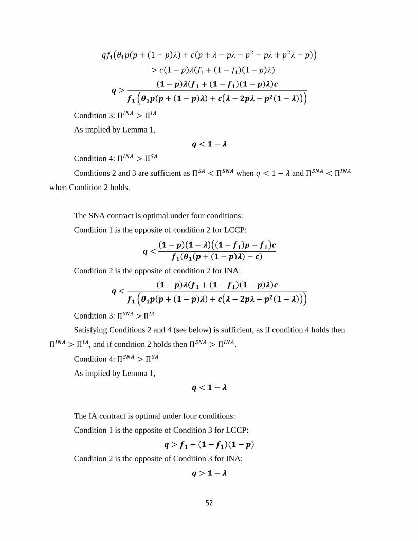
52

𝑞𝑓1(𝜃1𝑝(𝑝 + (1 − 𝑝)𝜆) + 𝑐(𝑝 + 𝜆 − 𝑝𝜆 − 𝑝2 − 𝑝𝜆 + 𝑝2𝜆 − 𝑝))

> 𝑐(1 − 𝑝)𝜆(𝑓1 + (1 − 𝑓1)(1 − 𝑝)𝜆)

𝒒 >(𝟏 − 𝒑)𝝀(𝒇𝟏 + (𝟏 − 𝒇𝟏)(𝟏 − 𝒑)𝝀)𝒄

𝒇𝟏 (𝜽𝟏𝒑(𝒑 + (𝟏 − 𝒑)𝝀) + 𝒄(𝝀 − 𝟐𝒑𝝀 − 𝒑𝟐(𝟏 − 𝝀)))

Condition 3: Π𝐼𝑁𝐴 > Π𝐼𝐴

As implied by Lemma 1,

𝒒 < 𝟏 − 𝝀

Condition 4: Π𝐼𝑁𝐴 > Π𝑆𝐴

Conditions 2 and 3 are sufficient as Π𝑆𝐴 < Π𝑆𝑁𝐴 when 𝑞 < 1 − 𝜆 and Π𝑆𝑁𝐴 < Π𝐼𝑁𝐴

when Condition 2 holds.

The SNA contract is optimal under four conditions:

Condition 1 is the opposite of condition 2 for LCCP:

𝒒 <(𝟏 − 𝒑)(𝟏 − 𝝀)((𝟏 − 𝒇𝟏)𝒑 − 𝒇𝟏)𝒄

𝒇𝟏(𝜽𝟏(𝒑 + (𝟏 − 𝒑)𝝀) − 𝒄)

Condition 2 is the opposite of condition 2 for INA:

𝒒 <(𝟏 − 𝒑)𝝀(𝒇𝟏 + (𝟏 − 𝒇𝟏)(𝟏 − 𝒑)𝝀)𝒄

𝒇𝟏 (𝜽𝟏𝒑(𝒑 + (𝟏 − 𝒑)𝝀) + 𝒄(𝝀 − 𝟐𝒑𝝀 − 𝒑𝟐(𝟏 − 𝝀)))

Condition 3: Π𝑆𝑁𝐴 > Π𝐼𝐴

Satisfying Conditions 2 and 4 (see below) is sufficient, as if condition 4 holds then

Π𝐼𝑁𝐴 > Π𝐼𝐴, and if condition 2 holds then Π𝑆𝑁𝐴 > Π𝐼𝑁𝐴.

Condition 4: Π𝑆𝑁𝐴 > Π𝑆𝐴

As implied by Lemma 1,

𝒒 < 𝟏 − 𝝀

The IA contract is optimal under four conditions:

Condition 1 is the opposite of Condition 3 for LCCP:

𝒒 > 𝒇𝟏 + (𝟏 − 𝒇𝟏)(𝟏 − 𝒑)

Condition 2 is the opposite of Condition 3 for INA:

𝒒 > 𝟏 − 𝝀

53

Condition 3: Π𝐼𝐴 > Π𝑆𝑁𝐴

Conditions 2 and 4 holding are sufficient for Condition 3 to hold, as Condition 2 implies

Π𝑆𝐴 > Π𝑆𝑁𝐴 and Condition 4 states Π𝐼𝐴 > Π𝐼𝑁𝐴.

Condition 4: Π𝐼𝐴 > Π𝑆𝐴

𝑓1 (𝜃1 − (1 − 𝑞(1 − 𝑝))𝑐

𝑝) + (1 − 𝑓1) (𝜃2 − (1 − 𝑝)Δ𝜃 − (1 − 𝑞)

1 − 𝑝

𝑝𝑐)

> 𝑓1(1 − 𝑞) (𝜃1 −𝑐

𝑝 + (1 − 𝑝)𝜆)

+ (1 − 𝑓1) (𝜃2 − Δ𝜃(1 − 𝑝) −(1 − 𝑞)(1 − 𝑝)

𝑝 + (1 − 𝑝)𝜆𝑐)

𝑓1 (𝜃1𝑞 +(1 − 𝑞)𝑐

𝑝 + (1 − 𝑝)𝜆−

(1 − 𝑞 + 𝑞𝑝)𝑐

𝑝) > (1 − 𝑓1)(1 − 𝑞)(1 − 𝑝)𝑐 (

1

𝑝−

1

𝑝 + (1 − 𝑝)𝜆)

𝑞 (𝑓1 (𝜃1 −𝑐

𝑝 + (1 − 𝑝)𝜆+

𝑐(1 − 𝑝)

𝑝) + (1 − 𝑓1)(1 − 𝑝)𝑐 (

1

𝑝−

1

𝑝 + (1 − 𝑝)𝜆))

> 𝑓1 (𝑐

𝑝−

𝑐

𝑝 + (1 − 𝑝)𝜆) + (1 − 𝑓1)(1 − 𝑝) (

𝑐

𝑝−

𝑐

𝑝 + (1 − 𝑝)𝜆)

𝑞 (𝑓1 (𝜃1𝑝(𝑝 + (1 − 𝑝)𝜆) − 𝑐(𝑝 − (1 − 𝑝)(𝑝 + (1 − 𝑝)𝜆)))

+ (1 − 𝑓1)(1 − 𝑝)𝑐(𝑝 + (1 − 𝑝)𝜆 − 𝑝))

> 𝑓1𝑐(𝑝 + (1 − 𝑝)𝜆 − 𝑝) + (1 − 𝑓1)(1 − 𝑝)𝑐(𝑝 + (1 − 𝑝)𝜆 − 𝑝)

𝑞 (𝑓1(𝑝(𝑝 + (1 − 𝑝)𝜆))(𝜃1 − 𝑐) + 𝑐(1 − 𝑝)𝜆(𝑓1 + (1 − 𝑓1)(1 − 𝑝)))

> 𝑐(1 − 𝑝)𝜆) (𝑓1 + (1 − 𝑓1)(1 − 𝑝))

𝒒 >(𝟏 − 𝒑)𝝀(𝒇𝟏 + (𝟏 − 𝒇𝟏)(𝟏 − 𝒑))𝒄

(𝟏 − 𝒑)𝝀(𝒇𝟏 + (𝟏 − 𝒇𝟏)(𝟏 − 𝒑))𝒄 + 𝒇𝟏(𝒑(𝒑 + (𝟏 − 𝒑)𝝀))(𝜽𝟏 − 𝒄)

For the SA contract to be optimal, it must satisfy the following four conditions:

Condition 1 is the opposite of Condition 4 for LCCP:

𝒒 >(𝟏 − 𝒑)(𝟏 − 𝝀)(𝒇𝟏 + (𝟏 − 𝒇𝟏)(𝟏 − 𝒑))𝒄

(𝟏 − 𝒑)(𝟏 − 𝝀)(𝒇𝟏 + (𝟏 − 𝒇𝟏)(𝟏 − 𝒑))𝒄 + (𝟏 − 𝒇𝟏)(𝒑 + (𝟏 − 𝒑)𝝀)𝒄 − 𝒇𝟏(𝜽𝟏 − 𝒄)

Condition 2: Π𝑆𝐴 > Π𝐼𝑁𝐴

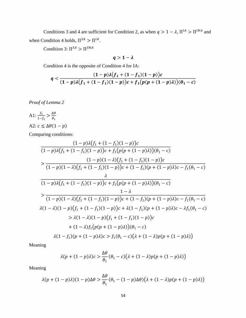
54

Conditions 3 and 4 are sufficient for Condition 2, as when 𝑞 > 1 − 𝜆, Π𝐼𝐴 > Π𝐼𝑁𝐴 and

when Condition 4 holds, Π𝑆𝐴 > Π𝐼𝐴.

Condition 3: Π𝑆𝐴 > Π𝑆𝑁𝐴

𝒒 > 𝟏 − 𝝀

Condition 4 is the opposite of Condition 4 for IA:

𝒒 <(𝟏 − 𝒑)𝝀(𝒇𝟏 + (𝟏 − 𝒇𝟏)(𝟏 − 𝒑))𝒄

(𝟏 − 𝒑)𝝀(𝒇𝟏 + (𝟏 − 𝒇𝟏)(𝟏 − 𝒑))𝒄 + 𝒇𝟏(𝒑(𝒑 + (𝟏 − 𝒑)𝝀))(𝜽𝟏 − 𝒄)

Proof of Lemma 2

A1: 𝑓1

1−𝑓1>

Δ𝜃

𝜃1

A2: 𝑐 ≤ Δ𝜃(1 − 𝑝)

Comparing conditions:

(1 − 𝑝)𝜆(𝑓1 + (1 − 𝑓1)(1 − 𝑝))𝑐

(1 − 𝑝)𝜆(𝑓1 + (1 − 𝑓1)(1 − 𝑝))𝑐 + 𝑓1(𝑝(𝑝 + (1 − 𝑝)𝜆))(𝜃1 − 𝑐)

>(1 − 𝑝)(1 − 𝜆)(𝑓1 + (1 − 𝑓1)(1 − 𝑝))𝑐

(1 − 𝑝)(1 − 𝜆)(𝑓1 + (1 − 𝑓1)(1 − 𝑝))𝑐 + (1 − 𝑓1)(𝑝 + (1 − 𝑝)𝜆)𝑐 − 𝑓1(𝜃1 − 𝑐)

𝜆

(1 − 𝑝)𝜆(𝑓1 + (1 − 𝑓1)(1 − 𝑝))𝑐 + 𝑓1(𝑝(𝑝 + (1 − 𝑝)𝜆))(𝜃1 − 𝑐)

>1 − 𝜆

(1 − 𝑝)(1 − 𝜆)(𝑓1 + (1 − 𝑓1)(1 − 𝑝))𝑐 + (1 − 𝑓1)(𝑝 + (1 − 𝑝)𝜆)𝑐 − 𝑓1(𝜃1 − 𝑐)

𝜆(1 − 𝜆)(1 − 𝑝)(𝑓1 + (1 − 𝑓1)(1 − 𝑝))𝑐 + 𝜆(1 − 𝑓1)(𝑝 + (1 − 𝑝)𝜆)𝑐 − 𝜆𝑓1(𝜃1 − 𝑐)

> 𝜆(1 − 𝜆)(1 − 𝑝)(𝑓1 + (1 − 𝑓1)(1 − 𝑝))𝑐

+ (1 − 𝜆)𝑓1(𝑝(𝑝 + (1 − 𝑝)𝜆))(𝜃1 − 𝑐)

𝜆(1 − 𝑓1)(𝑝 + (1 − 𝑝)𝜆)𝑐 > 𝑓1(𝜃1 − 𝑐)(𝜆 + (1 − 𝜆)𝑝(𝑝 + (1 − 𝑝)𝜆))

Meaning

𝜆(𝑝 + (1 − 𝑝)𝜆)𝑐 >Δ𝜃

𝜃1

(𝜃1 − 𝑐)(𝜆 + (1 − 𝜆)𝑝(𝑝 + (1 − 𝑝)𝜆))

Meaning

𝜆(𝑝 + (1 − 𝑝)𝜆)(1 − 𝑝)Δ𝜃 >Δ𝜃

𝜃1

(𝜃1 − (1 − 𝑝)Δ𝜃)(𝜆 + (1 − 𝜆)𝑝(𝑝 + (1 − 𝑝)𝜆))

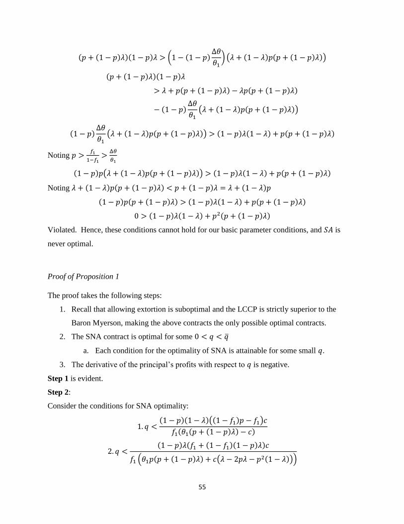
55

(𝑝 + (1 − 𝑝)𝜆)(1 − 𝑝)𝜆 > (1 − (1 − 𝑝)Δ𝜃

𝜃1) (𝜆 + (1 − 𝜆)𝑝(𝑝 + (1 − 𝑝)𝜆))

(𝑝 + (1 − 𝑝)𝜆)(1 − 𝑝)𝜆

> 𝜆 + 𝑝(𝑝 + (1 − 𝑝)𝜆) − 𝜆𝑝(𝑝 + (1 − 𝑝)𝜆)

− (1 − 𝑝)Δ𝜃

𝜃1(𝜆 + (1 − 𝜆)𝑝(𝑝 + (1 − 𝑝)𝜆))

(1 − 𝑝)Δ𝜃

𝜃1(𝜆 + (1 − 𝜆)𝑝(𝑝 + (1 − 𝑝)𝜆)) > (1 − 𝑝)𝜆(1 − 𝜆) + 𝑝(𝑝 + (1 − 𝑝)𝜆)

Noting 𝑝 >𝑓1

1−𝑓1>

Δ𝜃

𝜃1

(1 − 𝑝)𝑝(𝜆 + (1 − 𝜆)𝑝(𝑝 + (1 − 𝑝)𝜆)) > (1 − 𝑝)𝜆(1 − 𝜆) + 𝑝(𝑝 + (1 − 𝑝)𝜆)

Noting 𝜆 + (1 − 𝜆)𝑝(𝑝 + (1 − 𝑝)𝜆) < 𝑝 + (1 − 𝑝)𝜆 = 𝜆 + (1 − 𝜆)𝑝

(1 − 𝑝)𝑝(𝑝 + (1 − 𝑝)𝜆) > (1 − 𝑝)𝜆(1 − 𝜆) + 𝑝(𝑝 + (1 − 𝑝)𝜆)

0 > (1 − 𝑝)𝜆(1 − 𝜆) + 𝑝2(𝑝 + (1 − 𝑝)𝜆)

Violated. Hence, these conditions cannot hold for our basic parameter conditions, and 𝑆𝐴 is

never optimal.

Proof of Proposition 1

The proof takes the following steps:

1. Recall that allowing extortion is suboptimal and the LCCP is strictly superior to the

Baron Myerson, making the above contracts the only possible optimal contracts.

2. The SNA contract is optimal for some 0 < 𝑞 < �̅�

a. Each condition for the optimality of SNA is attainable for some small 𝑞.

3. The derivative of the principal’s profits with respect to 𝑞 is negative.

Step 1 is evident.

Step 2:

Consider the conditions for SNA optimality:

1. 𝑞 <(1 − 𝑝)(1 − 𝜆)((1 − 𝑓1)𝑝 − 𝑓1)𝑐

𝑓1(𝜃1(𝑝 + (1 − 𝑝)𝜆) − 𝑐)

2. 𝑞 <(1 − 𝑝)𝜆(𝑓1 + (1 − 𝑓1)(1 − 𝑝)𝜆)𝑐

𝑓1 (𝜃1𝑝(𝑝 + (1 − 𝑝)𝜆) + 𝑐(𝜆 − 2𝑝𝜆 − 𝑝2(1 − 𝜆)))

56

3. 𝑞 < 1 − 𝜆

As long as the numerators and denominators are positive these are the true conditions.

Condition 1

Numerator:

Note that 𝑝 >𝑓1

1−𝑓1 by earlier assumption. Therefore (1 − 𝑓1)𝑝 > 𝑓1, and the numerator is

positive.

Denominator is positive if

𝑐 ≤ 𝜃1(𝑝 + (1 − 𝑝)𝜆)

Which is required to avoid total shutdown for the low type in all the bribery-allowed cases.

Since both the numerator and denominator in Condition 1 are positive, there is some �̅� such that

𝑞1̅̅̅ =(1 − 𝑝)(1 − 𝜆)((1 − 𝑓1)𝑝 − 𝑓1)𝑐

𝑓1(𝜃1(𝑝 + (1 − 𝑝)𝜆) − 𝑐)

And therefore Condition 1 is met for 0 < 𝑞 < 𝑞1̅̅̅

Condition 2

Numerator: (1 − 𝑝)𝜆(𝑓1 + (1 − 𝑓1)(1 − 𝑝)𝜆)𝑐 > 0

Denominator: 𝑓1 (𝜃1𝑝(𝑝 + (1 − 𝑝)𝜆) + 𝑐(𝜆 − 2𝑝𝜆 − 𝑝2(1 − 𝜆)))

Re-writing: 𝑓1 (𝜃1𝑝(𝑝 + (1 − 𝑝)𝜆) + 𝑐((1 − 𝑝)(𝑝 + (1 − 𝑝)𝜆) − 𝑝))

𝑓1(𝑝(𝜃1(𝑝 + (1 − 𝑝)𝜆) − 𝑐) + 𝑐(1 − 𝑝)(𝑝 + (1 − 𝑝)𝜆))

𝑐 ≤ 𝜃1(𝑝 + (1 − 𝑝)𝜆)

Meaning 𝑓1 (𝜃1𝑝(𝑝 + (1 − 𝑝)𝜆) + 𝑐((1 − 𝑝)(𝑝 + (1 − 𝑝)𝜆) − 𝑝)) > 0

Since both the numerator and denominator in Condition 2 are positive, there is some �̅� such that

𝑞2̅̅ ̅ =(1 − 𝑝)𝜆(𝑓1 + (1 − 𝑓1)(1 − 𝑝)𝜆)𝑐

𝑓1 (𝜃1𝑝(𝑝 + (1 − 𝑝)𝜆) + 𝑐(𝜆 − 2𝑝𝜆 − 𝑝2(1 − 𝜆)))

And therefore Condition 2 is met for 0 < 𝑞 < 𝑞2̅̅ ̅

Condition 3

Clearly 1 − 𝜆 > 0

So for 𝑞3̅̅ ̅ = 1 − 𝜆, Condition 3 is met for 0 < 𝑞 < 𝑞3̅̅ ̅.

Set �̅�𝑚 = min(�̅�1, �̅�2, �̅�3)

The SNA contract is optimal for 0 < 𝑞 < �̅�𝑚, �̅�𝑚 > 0

57

Step 3:

The SNA profits are:

𝑓1(1 − 𝑞) (𝜃1 −𝑐

𝑝 + (1 − 𝑝)𝜆) + (1 − 𝑓1) (𝜃2 − (1 − 𝑝)Δ𝜃 −

(1 − 𝑝)𝜆

𝑝 + (1 − 𝑝)𝜆𝑐)

The derivative of the SNA profits with respect to 𝑞 are:

−𝑓1 (𝜃1 −𝑐

𝑝 + (1 − 𝑝)𝜆) < 0

Honesty hurts the principal in the SNA contract. The SNA contract is optimal for 0 < 𝑞 < �̅�𝑚.

Therefore honesty hurts the principal for 0 < 𝑞 < �̅�𝑚.

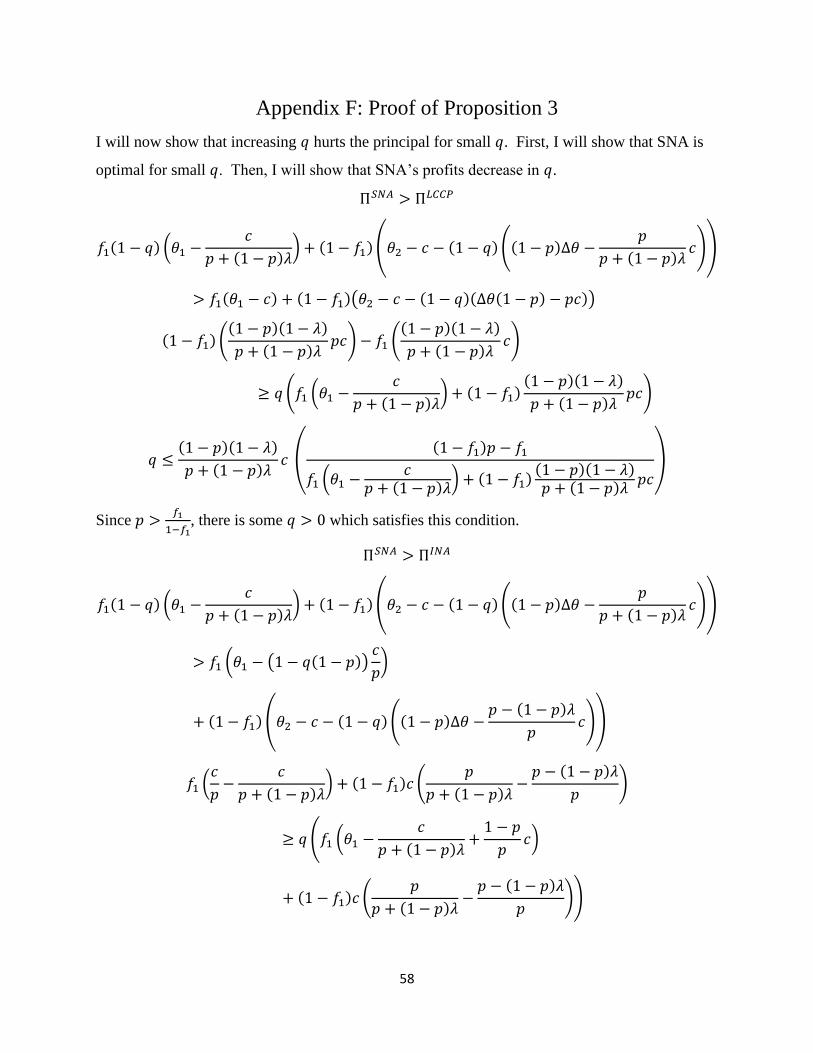
58

Appendix F: Proof of Proposition 3

I will now show that increasing 𝑞 hurts the principal for small 𝑞. First, I will show that SNA is

optimal for small 𝑞. Then, I will show that SNA’s profits decrease in 𝑞.

Π𝑆𝑁𝐴 > Π𝐿𝐶𝐶𝑃

𝑓1(1 − 𝑞) (𝜃1 −𝑐

𝑝 + (1 − 𝑝)𝜆) + (1 − 𝑓1) (𝜃2 − 𝑐 − (1 − 𝑞) ((1 − 𝑝)Δ𝜃 −

𝑝

𝑝 + (1 − 𝑝)𝜆𝑐))

> 𝑓1(𝜃1 − 𝑐) + (1 − 𝑓1)(𝜃2 − 𝑐 − (1 − 𝑞)(Δ𝜃(1 − 𝑝) − 𝑝𝑐))

(1 − 𝑓1) ((1 − 𝑝)(1 − 𝜆)

𝑝 + (1 − 𝑝)𝜆𝑝𝑐) − 𝑓1 (

(1 − 𝑝)(1 − 𝜆)

𝑝 + (1 − 𝑝)𝜆𝑐)

≥ 𝑞 (𝑓1 (𝜃1 −𝑐

𝑝 + (1 − 𝑝)𝜆) + (1 − 𝑓1)

(1 − 𝑝)(1 − 𝜆)

𝑝 + (1 − 𝑝)𝜆𝑝𝑐)

𝑞 ≤(1 − 𝑝)(1 − 𝜆)

𝑝 + (1 − 𝑝)𝜆𝑐 (

(1 − 𝑓1)𝑝 − 𝑓1

𝑓1 (𝜃1 −𝑐

𝑝 + (1 − 𝑝)𝜆) + (1 − 𝑓1)

(1 − 𝑝)(1 − 𝜆)𝑝 + (1 − 𝑝)𝜆

𝑝𝑐)

Since 𝑝 >𝑓1

1−𝑓1, there is some 𝑞 > 0 which satisfies this condition.

Π𝑆𝑁𝐴 > Π𝐼𝑁𝐴

𝑓1(1 − 𝑞) (𝜃1 −𝑐

𝑝 + (1 − 𝑝)𝜆) + (1 − 𝑓1) (𝜃2 − 𝑐 − (1 − 𝑞) ((1 − 𝑝)Δ𝜃 −

𝑝

𝑝 + (1 − 𝑝)𝜆𝑐))

> 𝑓1 (𝜃1 − (1 − 𝑞(1 − 𝑝))𝑐

𝑝)

+ (1 − 𝑓1) (𝜃2 − 𝑐 − (1 − 𝑞) ((1 − 𝑝)Δ𝜃 −𝑝 − (1 − 𝑝)𝜆

𝑝𝑐))

𝑓1 (𝑐

𝑝−

𝑐

𝑝 + (1 − 𝑝)𝜆) + (1 − 𝑓1)𝑐 (

𝑝

𝑝 + (1 − 𝑝)𝜆−

𝑝 − (1 − 𝑝)𝜆

𝑝)

≥ 𝑞 (𝑓1 (𝜃1 −𝑐

𝑝 + (1 − 𝑝)𝜆+

1 − 𝑝

𝑝𝑐)

+ (1 − 𝑓1)𝑐 (𝑝

𝑝 + (1 − 𝑝)𝜆−

𝑝 − (1 − 𝑝)𝜆

𝑝))

59

𝑝

𝑝 + (1 − 𝑝)𝜆−

𝑝 − (1 − 𝑝)𝜆

𝑝=

𝑝2 − (𝑝2 − 𝑝(1 − 𝑝)𝜆 + 𝑝(1 − 𝑝)𝜆 − (1 − 𝑝)2𝜆2)

𝑝(𝑝 + (1 − 𝑝)𝜆)

=(1 − 𝑝)2𝜆2

𝑝(𝑝 + (1 − 𝑝)𝜆

𝑐(1 − 𝑝)𝜆(𝑓1 + (1 − 𝑓1)(1 − 𝑝)𝜆)

≥ 𝑞 (𝜃1𝑓1𝑝(𝑝 + (1 − 𝑝)𝜆)

+ 𝑐(𝑓1((1 − 𝑝)(𝑝 + (1 − 𝑝)𝜆) − 𝑝) + (1 − 𝑓1)(1 − 𝑝)2𝜆2))

𝑐(1 − 𝑝)𝜆(𝑓1 + (1 − 𝑓1)(1 − 𝑝)𝜆)

≥ 𝑞(𝜃1𝑓1𝑝(𝑝 + (1 − 𝑝)𝜆) + 𝑐(𝑓1((1 − 𝑝)2𝜆 − 𝑝2) + (1 − 𝑓1)(1 − 𝑝)2𝜆2))

𝑞 ≤𝑐(1 − 𝑝)𝜆(𝑓1 + (1 − 𝑓1)(1 − 𝑝)𝜆)

𝜃1𝑓1𝑝(𝑝 + (1 − 𝑝)𝜆) + 𝑐(𝑓1((1 − 𝑝)2𝜆 − 𝑝2) + (1 − 𝑓1)(1 − 𝑝)2𝜆2)

The denominator is positive, and hence this holds from some 𝑞 > 0.

Hence, the SNA contract is optimal for small 𝑞.

𝑑Π𝑆𝑁𝐴

𝑑𝑞=

𝑑

𝑑𝑞[𝑓1(1 − 𝑞) (𝜃1 −

𝑐

𝑝 + (1 − 𝑝)𝜆)

+ (1 − 𝑓1) (𝜃2 − 𝑐 − (1 − 𝑞) ((1 − 𝑝)Δ𝜃 −𝑝

𝑝 + (1 − 𝑝)𝜆𝑐))]

𝑑Π𝑆𝑁𝐴

𝑑𝑞= −𝑓1 (𝜃1 −

𝑐

𝑝 + (1 − 𝑝)𝜆) + (1 − 𝑓1) ((1 − 𝑝)Δ𝜃 −

𝑝

𝑝 + (1 − 𝑝)𝜆𝑐)

𝑑Π𝑆𝑁𝐴

𝑑𝑞< 0

(1 − 𝑓1) ((1 − 𝑝)Δ𝜃 −𝑝

𝑝 + (1 − 𝑝)𝜆𝑐) < 𝑓1 (𝜃1 −

𝑐

𝑝 + (1 − 𝑝)𝜆)

Re-writing A1-A3

1 −𝑐

Δ𝜃> 𝑝 >

𝑓1

1 − 𝑓1>

𝛥𝜃

𝜃1

I will make substitutions using these parameter constraints to tighten the inequality, and

show that it can still hold.

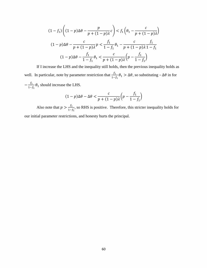
60

(1 − 𝑓1) ((1 − 𝑝)Δ𝜃 −𝑝

𝑝 + (1 − 𝑝)𝜆𝑐) < 𝑓1 (𝜃1 −

𝑐

𝑝 + (1 − 𝑝)𝜆)

(1 − 𝑝)Δ𝜃 −𝑐

𝑝 + (1 − 𝑝)𝜆𝑝 <

𝑓1

1 − 𝑓1𝜃1 −

𝑐

𝑝 + (1 − 𝑝)𝜆

𝑓1

1 − 𝑓1

(1 − 𝑝)Δ𝜃 −𝑓1

1 − 𝑓1𝜃1 <

𝑐

𝑝 + (1 − 𝑝)𝜆(𝑝 −

𝑓1

1 − 𝑓1)

If I increase the LHS and the inequality still holds, then the previous inequality holds as

well. In particular, note by parameter restriction that 𝑓1

1−𝑓1𝜃1 > Δ𝜃, so substituting – Δ𝜃 in for

−𝑓1

1−𝑓1𝜃1 should increase the LHS.

(1 − 𝑝)Δ𝜃 − Δ𝜃 <𝑐

𝑝 + (1 − 𝑝)𝜆(𝑝 −

𝑓1

1 − 𝑓1)

Also note that 𝑝 >𝑓1

1−𝑓1, so RHS is positive. Therefore, this stricter inequality holds for

our initial parameter restrictions, and honesty hurts the principal.

61

References

Acemoglu, Daron, and Thierry Verdier. "The choice between market failures and corruption."

American economic review (2000): 194-211.

Alger, Ingela, and Regis Renault. "Screening ethics when honest agents keep their word."

Economic theory 30.2 (2007): 291-311.

Andreoni, James, Brian Erard, and Jonathan Feinstein. "Tax compliance." Journal of economic

literature (1998): 818-860.

Auriol, Emmanuelle. "Corruption in procurement and public purchase." International Journal of

Industrial Organization 24.5 (2006): 867-885.

Che, Yeon-Koo. "Revolving doors and the optimal tolerance for agency collusion." The Rand

journal of economics (1995): 378-397.

Citizens United v. Federal Election Com'n, 130 S. Ct. 876, 558 U.S. 310, 175 L. Ed. 2d 753 (2010).

Cooray, Arusha V., and Friedrich Schneider. "Does corruption promote emigration? An empirical

examination." (2014).

De Haas, Hein. "Remittances, migration and social development." A Conceptual Review of the

Literature (2007).

Dincer, Oguzhan C., and Burak Gunalp. "Corruption and income inequality in the United States."

Contemporary Economic Policy 30.2 (2012): 283-292.

Dimant, Eugen, Tim Krieger, and Daniel Meierrieks. "The effect of corruption on migration,

1985–2000." Applied Economics Letters 20.13 (2013): 1270-1274.

Figalli, Alessio, Young-Heon Kim, and Robert J. McCann. "When is multidimensional screening

a convex program?." Journal of Economic Theory 146.2 (2011): 454-478.

Gupta, Sanjeev, Hamid Davoodi, and Rosa Alonso-Terme. "Does corruption affect income

inequality and poverty?." Economics of governance 3.1 (2002): 23-45.

Khalil, Fahad, and Jacques Lawarrée. "INCENTIVES FOR CORRUPTIBLE AUDITORS IN

THE ABSENCE OF COMMITMENT*." The Journal of Industrial Economics 54.2 (2006): 269-

291.

Khalil, Fahad, Jacques Lawarrée, and Sungho Yun. "Bribery versus extortion: allowing the lesser

of two evils." The RAND Journal of Economics 41.1 (2010): 179-198.

Kim, Mike. Escaping North Korea: Defiance and hope in the world's most repressive country.

Rowman & Littlefield, 2010.

62

Kofman, Fred, and Jacques Lawarrée. "Collusion in hierarchical agency." Econometrica: Journal

of the Econometric Society (1993): 629-656.

Kofman, Fred, and Jacques Lawarrée. "On the optimality of allowing collusion." Journal of Public

Economics 61.3 (1996): 383-407.

Lambert-Mogiliansky, Ariane. "On optimality of illegal collusion in contracts." Review of

Economic Design 3.4 (1998): 303-328.

Lambsdorff, Johann Graf. "Corruption and rent-seeking." Public choice 113.1-2 (2002): 97-125.

Manelli, Alejandro M., and Daniel R. Vincent. "Multidimensional mechanism design: Revenue

maximization and the multiple-good monopoly." Journal of Economic Theory 137.1 (2007): 153-

185.

Mittendorf, Brian. "Infectious ethics: How upright employees can ease concerns of tacit collusion."

Journal of Law, Economics, and Organization 24.2 (2008): 356-370.

Mookherjee, Dilip, and Ivan Paak-Liang Png. "Corruptible law enforcers: how should they be

compensated?." The Economic Journal (1995): 145-159.

Olsen, Trond E., and Gaute Torsvik. "Collusion and renegotiation in hierarchies: a case of

beneficial corruption." International Economic Review (1998): 413-438.

Rochet, Jean-Charles, and Philippe Choné. "Ironing, sweeping, and multidimensional screening."

Econometrica (1998): 783-826.

Scott, Troy J. "Equilibrium Extortion, Bargaining Power, and the Tradeoff between Informational

and Corruption Rents." Bargaining Power, and the Tradeoff between Informational and Corruption

Rents (June 8, 2014) (2014).

Severinov, Sergei, and Raymond Deneckere. "Screening when some agents are nonstrategic: does

a monopoly need to exclude?." The RAND Journal of Economics 37.4 (2006): 816-840.

Strausz, Roland. "Delegation of monitoring in a principal-agent relationship." The Review of

Economic Studies 64.3 (1997): 337-357.

Tirole, Jean. "Hierarchies and bureaucracies: On the role of collusion in organizations." Journal of

Law, Economics, & Organization (1986): 181-214.

Tirole, Jean. “Collusion and the theory of organizations,” in: Laffont, J.-J. (Ed).

Advances in Economic Theory, Vol.2 (1992), pp.151-206.

Yun, Sungho. "Costs of Engaging in Corruption: Equilibrium with Extortion and Framing." The

BE Journal of Economic Analysis & Policy 12.1 (2012).